Determinants of Industrial

Clusters in India

Ana M. Fernandes, World Bank

Gunjan Sharma, University of Missouri

This report is an output of the International Growth Centre.

High spatial concentration in Indian Manufacturing

• Manufacturing is much more concentrated in India than in other

developing and developed countries

State Share of Manufacturing Output (%)

State 1980 1990 2000 2007

Maharashtra 23.97 22.81 20.87 19.59

Gujrat 11.96 9.83 14.06 16.91

Tamil Nadu 10.86 10.06 10.41 9.03

WB 10.36 6.27 4.46 4.26

UP 6.14 9.40 6.97 7.78

Top 5 sum 63.29 58.37 56.77 57.57

Bihar 5.31 5.57 3.63 3.58

Andhra Pradesh 5.04 5.74 6.36 5.67

Karnataka 4.09 4.60 5.13 6.70

MP 4.07 5.48 5.62 5.14

Punjab 3.64 4.09 3.37 2.71

Top 10 Sum 85.43 83.85 80.88 81.37

Substantial variation in spatial concentration

• Spatial concentration varies substantially across industries and

states during an interesting period of major industrial policy

changes in India

▫ Industrial de-licensing in the 1980s and 1990s

▫ Trade reforms in the 1990s

▫ FDI liberalization in the 1990s

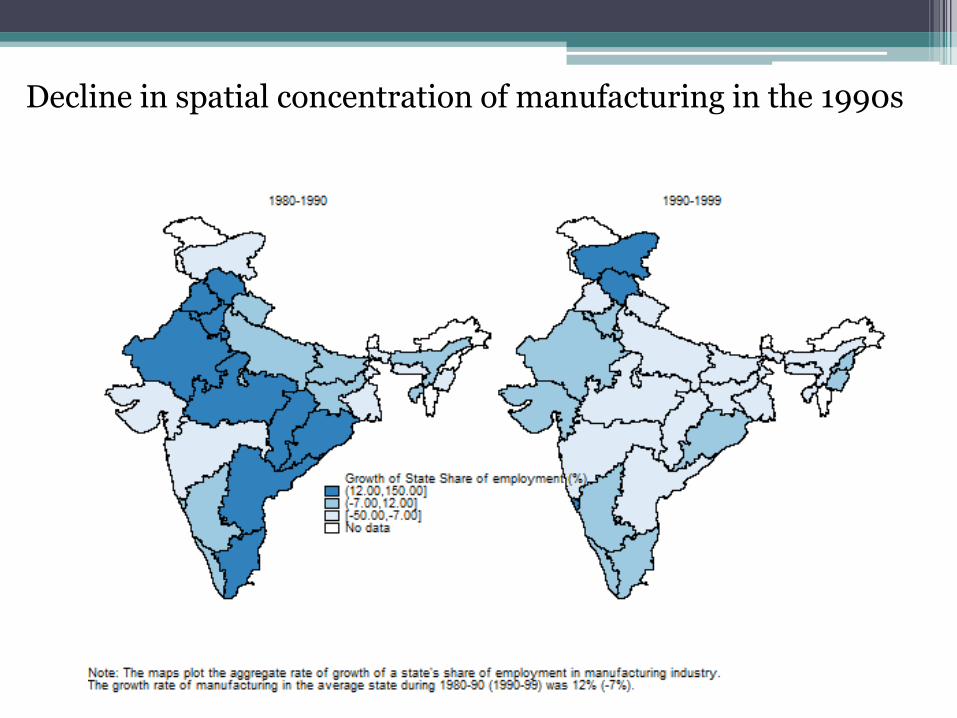
Decline in spatial concentration of manufacturing in the 1990s

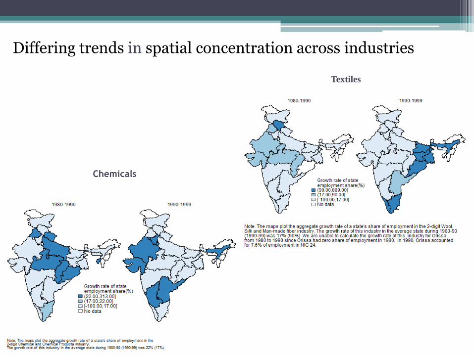
Textiles

Chemicals

Differing trends in spatial concentration across industries

Basic Questions

• What determines the location of different industries across states

within India?

▫ Our approach: econometrically estimate a model of comparative

advantage factors that can affect location choice (Midelfart-Knarvik,

Overman and Venables 2001)

▫ Comparative advantage: combination of region and industry

features

▫ Analyze both the stock (employment share of state-industry cell) and

flow (entry into a state-industry cell) location decisions

• Are there complementarities between regional and central

government initiatives to boost manufacturing industry?

▫ Estimate the effect of industrial policy on location choice

▫ Interact industrial policy with comparative advantage variables

Theoretical Background: New economic geography & trade theory

• Industries that intensively use intermediate industrial inputs tend

to locate in regions with a large industrial base (Venables 1996)

• Industries with IRS tend to locate in regions with large market

potentials (Krugman 1980, Helpman & Krugman 1985)

• Spatial distribution of production is determined by the spatial

distribution of natural resources (Leamer and Levinsohn 1995,

Heckscher-Ohlin model)

7

8

Comparative Advantage

Definition Proxy

BASEjst

IO linkages of j * Industrial base in s

𝑀𝑎𝑡𝑒𝑟𝑖𝑎𝑙𝑠𝑗𝑡𝑆𝑎𝑙𝑒𝑠𝑗𝑡

∗ 𝑀𝑎𝑛𝑓𝑠𝑡

𝑆𝐷𝑃𝑠𝑡

MKTjst IRS in j * Market potential of s

(Plant size)jt* Per capita SDPst

EDUjst Skill intensity of j * Skill abundance of s 𝑆𝑘𝑖𝑙𝑙𝑒𝑑 𝐿𝑗𝑡𝐿𝑗𝑡

∗ 𝑆𝑘𝑖𝑙𝑙𝑒𝑑 𝐿𝑠𝑡

𝐿𝑠𝑡

LABORjst

(Labor abundance)st * (Labor intensity)jt 𝑤𝐿𝑗𝑡

𝑌𝑗𝑡 * 𝑤𝑠𝑡 𝑤𝑡

INFRAjst Infrastructurest * (Transport intensity)jt

𝑇𝑟𝑎𝑛𝑠𝑝𝑜𝑟𝑡 𝐸𝑥𝑝𝑑𝑠𝑡

∗𝐼𝑛𝑣𝑒𝑛𝑡𝑜𝑟𝑦𝑗𝑡

𝑆𝑎𝑙𝑒𝑠𝑗𝑡

GOVERNjst (Contract intensity)jt * Governancest

𝑀𝑎𝑡𝑒𝑟𝑖𝑎𝑙𝑠𝑗𝑡𝑆𝑎𝑙𝑒𝑠𝑗𝑡

∗𝑀𝑢𝑟𝑑𝑒𝑟𝑠𝑡

𝑃𝑜𝑝 𝑠𝑡

Data – Spatial concentration of industries

• Annual Survey of Industries (ASI) cross-sections of

manufacturing plant-level data 1980-99

▫ Covers all factories registered under Factories Act of 1948

▫ ASI frame combines a ‘census sector’ and ‘sample sector’

▫ No survey conducted in 1995-96

▫ Compute LHS and industry-level RHS variables

• State-level GDP and population data: EPW Foundation

▫ Use gross SDP at 1993-94 prices

▫ Share of manufacturing in SDP

▫ State expenditure on transport and communication

• Governance:

▫ Murder rate per capita (Sharma, 2011)

LHS Variables

• 𝑆ℎ𝑎𝑟𝑒𝑗𝑠𝑡 =𝐿𝑗𝑠𝑡

𝐿𝑗𝑡=

𝐸𝑚𝑝𝑙𝑜𝑦𝑚𝑒𝑛𝑡 𝑖𝑛 𝑠𝑡𝑎𝑡𝑒 𝑠,𝑖𝑛𝑑𝑢𝑠𝑡𝑟𝑦 𝑗,𝑦𝑒𝑎𝑟 𝑡

𝐸𝑚𝑝𝑙𝑜𝑦𝑚𝑒𝑛𝑡 𝑖𝑛 𝑖𝑛𝑑𝑢𝑠𝑡𝑟𝑦 𝑗,𝑦𝑒𝑎𝑟 𝑡

• 𝐸𝑛𝑡𝑟𝑦𝑅𝑎𝑡𝑒𝑗𝑠𝑡 =𝐸𝑚𝑝𝑙𝑜𝑦𝑚𝑒𝑛𝑡 𝑖𝑛 1−3 𝑦𝑒𝑎𝑟 𝑜𝑙𝑑 𝑝𝑙𝑎𝑛𝑡𝑠𝑗𝑠𝑡

𝐿𝑗𝑠𝑡

• Another possibility

• 𝐸𝑛𝑡𝑟𝑦𝑆ℎ𝑎𝑟𝑒𝑗𝑠𝑡 =𝐸𝑚𝑝𝑙𝑜𝑦𝑚𝑒𝑛𝑡 𝑖𝑛 1−3 𝑦𝑒𝑎𝑟 𝑜𝑙𝑑 𝑝𝑙𝑎𝑛𝑡𝑠𝑗𝑠𝑡

𝐸𝑚𝑝𝑙𝑜𝑦𝑚𝑒𝑛𝑡 𝑖𝑛 1−3 𝑦𝑒𝑎𝑟 𝑜𝑙𝑑 𝑝𝑙𝑎𝑛𝑡𝑠𝑗𝑡

10

Data and econometric challenges

• Data only on formal sector

▫ Censored data: plants above a certain size are captured

▫ State-industry cells could be empty due to this censoring

• Geographic unit : State

▫ Can not identify anything smaller

• Many zeroes

▫ Not all industries locate in all states

▫ Ignore them: OLS

▫ Add small number to each empty cell

• Fractional nature of dependent variable

▫ Tobit

▫ FLOGIT (Papke and Wooldridge 1996) that takes account of the fractional

nature as well as of the zeros

11

12

Distribution in Maharashtra

13

Distribution in Rajasthan

14

15

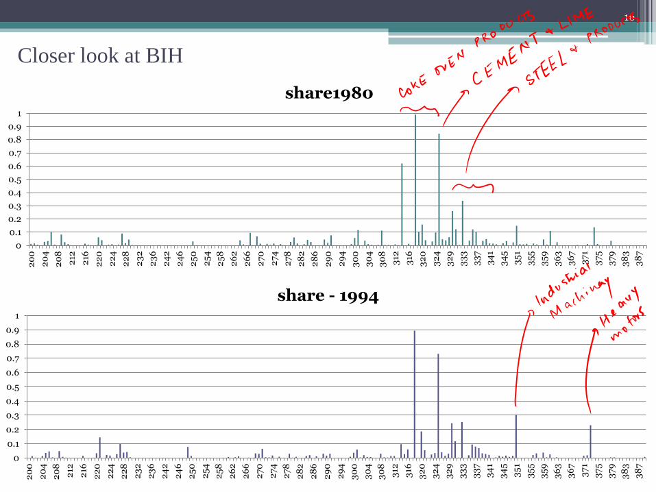
Closer look at BIH

16

0

0.1

0.2

0.3

0.4

0.5

0.6

0.7

0.8

0.9

1

20

0

20

4

20

8

212

216

22

0

22

4

22

8

23

2

23

6

24

2

24

6

25

0

25

4

25

8

26

2

26

6

27

0

27

4

27

8

28

2

28

6

29

0

29

4

30

0

30

4

30

8

312

316

32

0

32

4

32

9

33

3

33

7

34

1

34

5

35

1

35

5

35

9

36

3

36

7

37

1

37

5

37

9

38

3

38

7

share1980

0

0.1

0.2

0.3

0.4

0.5

0.6

0.7

0.8

0.9

1

20

0

20

4

20

8

212

216

22

0

22

4

22

8

23

2

23

6

24

2

24

6

25

0

25

4

25

8

26

2

26

6

27

0

27

4

27

8

28

2

28

6

29

0

29

4

30

0

30

4

30

8

312

316

32

0

32

4

32

9

33

3

33

7

34

1

34

5

35

1

35

5

35

9

36

3

36

7

37

1

37

5

37

9

38

3

38

7

share - 1994

17

0

0.1

0.2

0.3

0.4

0.5

0.6

0.7

0.8

0.9

20

0

20

4

20

8

212

216

22

0

22

4

22

8

23

2

23

6

24

2

24

6

25

0

25

4

25

8

26

2

26

6

27

0

27

4

27

8

28

2

28

6

29

0

29

4

30

0

30

4

30

8

312

316

32

0

32

4

32

9

33

3

33

7

34

1

34

5

35

1

35

5

35

9

36

3

36

7

37

1

37

5

37

9

38

3

38

7

share 2000

0

0.1

0.2

0.3

0.4

0.5

0.6

0.7

0.8

0.9

20

0

20

4

20

8

212

216

22

0

22

4

22

8

23

2

23

6

24

2

24

6

25

0

25

4

25

8

26

2

26

6

27

0

27

4

27

8

28

2

28

6

29

0

29

4

30

0

30

4

30

8

312

316

32

0

32

4

32

9

33

3

33

7

34

1

34

5

35

1

35

5

35

9

36

3

36

7

37

1

37

5

37

9

38

3

38

7

share - 2007

Specification

• Lag comparative advantage determinants

• Include 180 3-digit industry fixed effects, 17 state fixed effects, 18

year fixed effects

• Cluster standard error by industry

18

ln (𝑆ℎ𝑎𝑟𝑒)𝑗𝑠𝑡= 𝛼 +𝑀𝐾𝑇𝑗𝑠,𝑡−1 ∗ 𝛽1 + 𝐵𝐴𝑆𝐸𝑗𝑠,𝑡−1 ∗ 𝛽2 + 𝐸𝐷𝑈𝑗𝑠,𝑡−1 ∗ 𝛽3+ 𝐿𝐴𝐵𝑂𝑅𝑗𝑠,𝑡−1 ∗ 𝛽4 + 𝐼𝑁𝐹𝑅𝐴𝑗𝑠,𝑡−1 ∗ 𝛽5 + 𝐺𝑂𝑉𝐸𝑅𝑁𝑗𝑠,𝑡−1 ∗ 𝛽6 + 𝛿𝑗+ 𝜃𝑠 + 𝜇𝑡 + 휀𝑗𝑠𝑡

19

LHS = share

Ignore zeros Include zeros

OLS TOBIT FLOGIT OLS OLS on

share +e TOBIT FLOGIT

MKT -0.0758** -0.0021 -0.0350 -0.1692*** -0.0444** -0.0073** -0.0773*

(0.0350) (0.0039) (0.0411) (0.0442) (0.0221) (0.0033) (0.0442)

BASE 0.0103* -0.0012** -0.0117** -0.0044 -0.0059*** -0.0008** -0.0143***

(0.0056) (0.0005) (0.0051) (0.0073) (0.0016) (0.0003) (0.0049)

EDU 0.1216*** 0.0128*** 0.1401*** 0.1116** 0.0824*** 0.0110*** 0.1377***

(0.0344) (0.0033) (0.0332) (0.0473) (0.0253) (0.0030) (0.0335)

LABOR -0.3011 -0.2037*** -0.8070*** 0.0194*** 0.0063*** 0.0027 0.0259

(0.1970) (0.0466) (0.3089) (0.0032) (0.0020) (0.0038) (0.0336)

INFRA 0.0059 0.0001 0.0033 0.0186 0.0097 0.0004 0.0024

(0.0085) (0.0014) (0.0102) (0.0215) (0.0088) (0.0012) (0.0092)

GOVERN 0.0610 0.0074** 0.0638*** -0.0014 0.0383* 0.0031 0.0607***

(0.0510) (0.0033) (0.0165) (0.0548) (0.0224) (0.0030) (0.0219)

Cons -3.0867*** 0.1426*** -1.7754*** -5.6116*** -3.4503*** 0.0006 -2.6450***

(0.0815) (0.0081) (0.0996) (0.1386) (0.0680) (0.0088) (0.1069)

N 35902 36075 36075 58560 58386 58560 58560

R-sq 0.3490 0.5456 0.2991

20

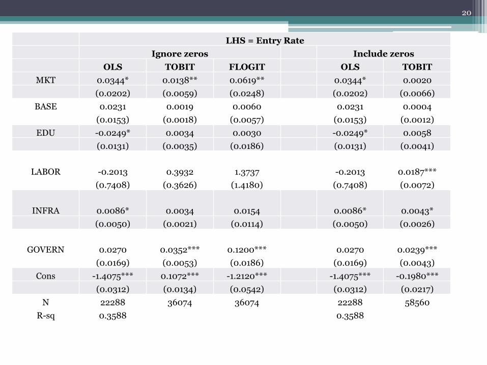
LHS = Entry Rate

Ignore zeros Include zeros

OLS TOBIT FLOGIT OLS TOBIT

MKT 0.0344* 0.0138** 0.0619** 0.0344* 0.0020

(0.0202) (0.0059) (0.0248) (0.0202) (0.0066)

BASE 0.0231 0.0019 0.0060 0.0231 0.0004

(0.0153) (0.0018) (0.0057) (0.0153) (0.0012)

EDU -0.0249* 0.0034 0.0030 -0.0249* 0.0058

(0.0131) (0.0035) (0.0186) (0.0131) (0.0041)

LABOR -0.2013 0.3932 1.3737 -0.2013 0.0187***

(0.7408) (0.3626) (1.4180) (0.7408) (0.0072)

INFRA 0.0086* 0.0034 0.0154 0.0086* 0.0043*

(0.0050) (0.0021) (0.0114) (0.0050) (0.0026)

GOVERN 0.0270 0.0352*** 0.1200*** 0.0270 0.0239***

(0.0169) (0.0053) (0.0186) (0.0169) (0.0043)

Cons -1.4075*** 0.1072*** -1.2120*** -1.4075*** -0.1980***

(0.0312) (0.0134) (0.0542) (0.0312) (0.0217)

N 22288 36074 36074 22288 58560

R-sq 0.3588 0.3588

The Adding Up Problem

• Both LHS variables add up to 1 when summed across states

▫ Unidentified/unaddressed problem in the literature

▫ Errors may have a structure within each industry

• Options

▫ Drop one state per industry

Implicitly doing that since we focus on 16 states for which we have state-

level data

▫ S.E. clustered around industry in all specifications so far

▫ Use levels instead of shares

L = Employment in cell jst

Entry = Employment in new plants in cell jst

21

Results for levels

LHS = Employment LHS = Entry Employment

OLS (logL) TOBIT OLS (log) TOBIT

MKT -0.1402*** -834.6254*** -0.0074 -63.9555

(0.0345) (235.9084) (0.0452) (130.0259)

BASE -0.0159** -75.1236 0.0097 -0.1836

(0.0061) (74.6013) (0.0248) (25.5150)

EDU 0.1111*** 1123.2231** 0.1302*** 315.2483**

(0.0341) (501.9722) (0.0298) (138.0189)

LABOR 0.4888** 418.7496 -0.0371 383.0108

(0.2320) (268.6748) (1.5799) (237.2959)

INFRA 0.0051 366.9056 -0.0077 63.2677

(0.0112) (257.9313) (0.0133) (62.1851)

GOVERN -0.0054 -232.8600 0.0227 247.1699

(0.0556) (301.0789) (0.0487) (167.1035)

LOBBY = Ljt * CONGRESSst 0.004** 7.39 -0.336* 6.14

(0.0016) (19.3) (0.002) (9.72)

Cons 4.9732*** -7537.2630*** 4.5953*** -9714.5629**

(0.0789) (1713.6057) (0.0863) (4949.7524)

N 35902 58560 22232 58560

R-sq 0.5364 0.3799

22

Specification 2

• Can industrial policy affect spatial distribution?

• Does industrial policy affect the relative strength of comparative

advantage forces?

▫ Are market oriented federal reforms complementary to state-level initiatives

(improved infrastructure, governance etc) aimed at attracting manufacturing

industry?

23

𝐿𝐻𝑆𝑗𝑠𝑡 = 𝛼 + 𝐶𝑜𝑚𝑝 𝐴𝑑𝑣𝑗𝑠,𝑡−1 ∗ 𝛽 + 𝑃𝑜𝑙𝑖𝑐𝑦𝑗,𝑡−1 ∗ 𝛾 + 𝐶𝑜𝑚𝑝 𝐴𝑑𝑣𝑗𝑠,𝑡−1∗ 𝑃𝑜𝑙𝑖𝑐𝑦𝑗,𝑡−1 ∗ 𝜋 + 𝛿𝑗 + 𝜃𝑠 + 𝜇𝑡 + 휀𝑗𝑠𝑡

India’s License “Raj”

• Draconian industrial licensing regime restricted entry and output

(Aghion et al., 2005; Chamarbagwala and Sharma, 2011)

▫ Licenses to continue or begin production were conditional on proposed

location of project and permission was required to change locations

▫ Explicitly used to spread manufacturing industry to backward areas,

particularly in the 1970s and 1980s (Marathe, 1989)

Effects of trade reform on spatial concentration

• New economic geography models – special case: assess the impact

of trade liberalization (= a reduction trade costs with respect to the

rest of the world) on the regional distribution of production within

a country

• Some models predict that manufacturing will concentrate after

trade liberalization for example in border regions or near ports

(Brülhart et al., 2004; Crozet and Koenig, 2004)

• Other models where congestion costs dominate predict that trade

reforms lead to less spatial concentration (Krugman and Elizondo,

1996; Behrens et al., 2007)

• Evidence for Argentina (Martincus and Sanguinetti, 2009)

Effects of FDI liberalization on spatial concentration

• Foreign firms want to take advantage of untapped domestic

consumer market => rise in dispersion (Amiti and Javorcik, 2008)

• But foreign firms relying on domestic IO linkages will locate

close to suppliers maybe already in clusters => rise in

concentration (Amiti and Javorcik, 2008)

• Entry of foreign firms leads to more competition for domestic

firms that may chose to locate away => rise in dispersion

• But if domestic firms become vertically linked to foreign firms

and these locate in clusters => rise in concentration

Average effect of policies

SHARE EMPLOYMENT ENTRY RATE ENTRY

EMPLOYMENT

DEL -0.0011* -217.8441 -0.0021 -17.8938

(0.0007) (152.2738) (0.0057) (92.7899)

FDI -0.0007** -81.9652 -0.0035 -43.0524

(0.0003) (66.6630) (0.0023) (42.7670)

TR 0.0001 131.2422 -0.0014 -9.4334

(0.0008) (255.9506) (0.0059) (129.5326)

27

• DEL and FDI reduce agglomeration. Consistent with Fernandes and Sharma (2010)

• All comparative advantage variables have signs and magnitudes consistent with earlier tables

Mechanisms through which policies work: Interactions

• Results for share and entry rate stronger than for total employment

and entry employment

• Share and total employment

▫ Rise with trade reform via MKT, INFRA

▫ Rise with FDI via BASE, EDU and GOVERN

▫ Rise with DEL via LABOR

▫ Fall with FDI and TR via LABOR

Import competing industries (K-intensive) get more K-intensive after

trade reforms

• Entry rate and entry employment

▫ Rise with FDI and TR via BASE, EDU, INFRA

▫ Rise with DEL via LABOR

▫ Fall with DEL via INFRA

28

Conclusions and caveats

• Comparative advantage factors important in explaining

concentration and entry

• Federal policies boost importance of some types of comparative

advantage

▫ Evidence more convincing for share rather than entry

▫ Incumbents benefitted more from reforms?

• Future

▫ Include 7 years of recent data

▫ Specifications that hold constant industry characteristics

▫ Model entry = number of new plants

▫ Model spatial concentration of informal sector

29

Conclusions and caveats

Cities and Economic Growth Conference, Dec 2010 30

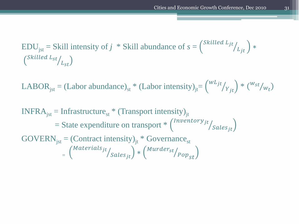
EDUjst = Skill intensity of j * Skill abundance of s = 𝑆𝑘𝑖𝑙𝑙𝑒𝑑 𝐿𝑗𝑡

𝐿𝑗𝑡 ∗

𝑆𝑘𝑖𝑙𝑙𝑒𝑑 𝐿𝑠𝑡 𝐿𝑠𝑡

LABORjst = (Labor abundance)st * (Labor intensity)jt= 𝑤𝐿𝑗𝑡

𝑌𝑗𝑡 * 𝑤𝑠𝑡

𝑤𝑡

INFRAjst = Infrastructurest * (Transport intensity)jt

= State expenditure on transport * 𝐼𝑛𝑣𝑒𝑛𝑡𝑜𝑟𝑦𝑗𝑡

𝑆𝑎𝑙𝑒𝑠𝑗𝑡

GOVERNjst = (Contract intensity)jt * Governancest

= 𝑀𝑎𝑡𝑒𝑟𝑖𝑎𝑙𝑠𝑗𝑡

𝑆𝑎𝑙𝑒𝑠𝑗𝑡 ∗ 𝑀𝑢𝑟𝑑𝑒𝑟𝑠𝑡

𝑃𝑜𝑝 𝑠𝑡

Cities and Economic Growth Conference, Dec 2010 31

COMPARATI

VE

ADVANTAGE POLICY OLS log(share)

OLS on

log(share+e)

FLOGIT,

robust SE

FLOGIT,

CLUSTER

MKT -0.0997*** -0.2288*** -0.1098*** -0.1098***

(0.0312) (0.0420) (0.0137) (0.0217)

DEL -0.0150 -0.0305 -0.0432*** -0.0432*

(0.0347) (0.0331) (0.0151) (0.0259)

FDI -0.0423 -0.1228* -0.0611 -0.0611*

(0.0388) (0.0694) (0.0404) (0.0371)

TRADE 0.0608 0.0671 0.0779*** 0.0779***

(0.0376) (0.0560) (0.0202) (0.0259)

BASE -0.0192 -0.0138 -0.0387** -0.0387

(0.0288) (0.0379) (0.0175) (0.0236)

FDI 0.0337 0.1816** 0.0466* 0.0466***

(0.0417) (0.0664) (0.0283) (0.0154)

EDU 0.1235*** 0.0906* 0.1390*** 0.1390***

(0.0340) (0.0455) (0.0112) (0.0251)

FDI 0.0426** 0.1019*** 0.0237* 0.0237

(0.0175) (0.0272) (0.0144) (0.0187)

LABOR 1.4556 -0.1849 0.2730 0.2730*

(0.8475) (0.3869) (0.1951) (0.1525)

DEL -0.0332 0.3122*** 0.5816*** 0.5816***

(0.4693) (0.0751) (0.1290) (0.1446)

TRADE -1.8236** -0.1815 -0.8955*** -0.8955**

(0.7099) (0.1726) (0.1711) (0.3783)

FDI 0.4497 -2.6716 -1.2226 -1.2226*

(1.5193) (2.6177) (1.2416) (0.7297)

INFRA 0.0013 -0.0264 -0.0126 -0.0126*

(0.0093) (0.0152) (0.0088) (0.0066)

TRADE 0.0056 0.0766*** 0.0243** 0.0243**

(0.0101) (0.0129) (0.0116) (0.0105)

GOVERN -0.0980 -0.2678*** -0.0831 -0.0831

(0.0741) (0.0766) (0.0521) (0.0534)

DEL -0.2631*** -0.4911*** -0.3064*** -0.3064***

(0.0656) (0.0756) (0.0624) (0.0366)

32

COMPARATIV

E ADVTANGE POLICY

OLS on

log(ENTRY)

OLS on

log(ENTRY+e) FLOGIT, robust

FLOGIT with

cluster(state)

BASE -0.0157 0.0155 0.0252 0.0252

(0.0317) (0.0198) (0.0238) (0.0294)

DEL -0.0391 0.0361** 0.1110*** 0.1110***

(0.0363) (0.0164) (0.0377) (0.0313)

FDI 0.0417** -0.0003 0.0607 0.0607**

(0.0190) (0.0136) (0.0412) (0.0251)

TRADE 0.0281 0.0562* 0.1430*** 0.1430***

(0.0762) (0.0290) (0.0516) (0.0430)

EDU 0.1323*** -0.0271 0.0004 0.0004

(0.0230) (0.0187) (0.0142) (0.0358)

FDI 0.0139 0.0050 0.0256 0.0256*

(0.0099) (0.0071) (0.0176) (0.0133)

LABOR 0.6680 -1.1903 0.3393 0.3393*

(2.2663) (1.3231) (0.2589) (0.2021)

DEL 0.1050 0.7105 0.5568** 0.5568***

(1.2641) (0.4202) (0.2820) (0.1334)

INFRA -0.0121 0.0063 0.0290** 0.0290**

(0.0146) (0.0070) (0.0145) (0.0125)

FDI -0.0051 -0.0018 0.0106 0.0106*

(0.0049) (0.0040) (0.0139) (0.0060)

33