Determinants of German FDI:New Evidence from Micro-Data

Claudia Buch(Kiel Institute for World Economics)

J�rn Kleinert(Kiel Institute for World Economics)

Farid Toubal(Kiel University, Department of Economics)

Discussion paper 09/03

Economic Research Centre

of the Deutsche Bundesbank

March 2003

The discussion papers published in this series representthe authors’ personal opinions and do not necessarily reflect the viewsof the Deutsche Bundesbank.

Deutsche Bundesbank, Wilhelm-Epstein-Strasse 14, 60431 Frankfurt am Main,Postfach 10 06 02, 60006 Frankfurt am Main

Tel +49 69 9566-1Telex within Germany 41227, telex from abroad 414431, fax +49 69 5601071

Please address all orders in writing to: Deutsche Bundesbank,Press and Public Relations Division, at the above address or via fax No. +49 69 9566-3077

Reproduction permitted only if source is stated.

ISBN 3–935821–52–2

Abstract

This paper provides new evidence on the foreign direct investment stocks of German firms.We use firm-level data for the years 1990-2000 to describe the regional and sectoralpatterns of German FDI through gravity-type equations. We provide evidence on thepatterns of FDI by sector, by size of the foreign affiliate, and by the number of affiliates perhost country. While market size and geographic distance have a significant impact on FDIstocks, we also find differences in the determinants of FDI between sectors as well asbetween the size of foreign affiliates and the number of foreign affiliates.

Keywords: distance coefficients, gravity equations, foreign direct investment JEL-classification: F0, F21 (99 words)

Zusammenfassung

Dieses Papier untersucht die Direktinvestitionsbestände deutscher multinationalerUnternehmen im Ausland auf drei verschiedenen Aggregationsniveaus. Dafür nutzen wireinen reichhaltigen Datensatz auf Unternehmensebene, der sektoral und auf Länderebeneaggregiert und als Mikrodatensatz analysiert wird. Unsere Analyse bezieht sich auf dieJahre 1990 bis 2000. Mittels eines Gravitätsansatzes beschreiben wir die sektoralen undregionalen Muster deutscher Direktinvestitionen im Ausland und diskutieren dieUnterschiede, die sich für die verschiedenen Aggregationsniveaus ergeben.

Contents

1. Motivation 1

2. The Data 2

2.1. Foreign Direct Investment 2

2.2. Explanatory Variables 4

3. Empirical Results 7

3.1. What Determines German FDI? 7

3.2. Do Determinants of FDI Differ Across Sectors? 9

3.3. What Determines the Size of Foreign Affiliates? 11

4. Avenues for Future Research 14

References 17

List of Tables and Figures

Tables

Table 1: Regional and Sectoral Breakdown of German FDI, End of 2000 20

Table 2: Quasi Panel Regressions 21

Table 3: Sectoral Regressions 22

Table 4a: Regressions Using Micro-Data – Baseline, Not Including Size and

Trade Effects 24

Table 4b: Regressions Using Micro-Data – Baseline, Including Size and Trade

Effects 25

Table 5a: Number of Foreign Affiliates – Baseline, Not Including Trade

Effects 26

Table 5b: Number of Foreign Affiliates – Baseline, Including Trade Effects 27

Table 6: Foreign Affiliates and Wholesale Trade 29

Figures

Figure 1: Sectoral Distance Coefficients 23

Figure 2: Average Size of Foreign Affiliates 28

Determinants of German FDI:New Evidence from Micro-Data*

1 Motivation

The globalization of markets has heightened interest in the determinants of firms’ foreigndirect investment (FDI) decisions. From a theoretical point of view, FDI decisions have beenanalyzed based on the eclectic paradigm (Dunning 1977), which distinguishes ownership,location, and internalization advantages of foreign investments.1 The new trade theory, whichessentially focuses on the ownership and location advantages, provides a more formalframework for analyzing FDI decisions. Part of this literature uses game theoreticalapproaches to explain the presence of multinationals by the existence of economies of scaleand oligopolistic market structures (Horstmann and Markusen 1992, Brainard 1993, Raff andSrinivasan 1998, Raff and Kim 1999). Activities of multinationals have also been modeledendogenously in general equilibrium models in which the activities of multinationals aredriven by country size, relative endowments, firm- and plant-level costs, and trade costs(Markusen and Venables 1998, 2000, Kleinert 2001). These ‘microeconomic’ theoreticalmodels are based on the decision of companies, which are all symmetric. This symmetryassumption allows analyzing a representative firm in each country in order to deriveimplications for aggregate FDI.

One way to test these models empirically has been to derive gravity models, which haveproven very useful in explaining patterns of international investments (see, e.g. Carr et al.2001 and Egger 2003). Most empirical applications are based on macroeconomic oraggregated data even though theoretical work has focused on explanations of internationalinvestments that use microeconomic approaches and that stress aspects of industrialorganization. However, analyzing foreign direct investment decisions on the basis ofaggregated data does not allow a number of interesting aspects to be studied. It is not possible,

* This paper has partly been written while the authors visited the Research Centre of the Deutsche Bundesbank.The hospitality of the Bundesbank and access to the micro-database “International Capital Links” aregratefully acknowledged. This project has benefited from financial support by the Thyssen Foundation. Theauthors would like to thank Heinz Herrmann, Joerg Doepke, Alexander Lipponer, Fred Ramb, Horst Raff,Harald Stahl as well as participants of seminars given at the Deutsche Bundesbank and at the University ofKiel for their support and for most helpful discussions. Roland Bodenstein, Marco Oestmann, and AnneRichter have provided efficient research assistance. All errors and inaccuracies are solely in our ownresponsibility.

1 For a survey of the literature see Markusen (1995).

– 1 –

for instance, to distinguish between firm-level and country-specific determinants of FDI, or toanalyze the behavior of small versus large foreign affiliates.

In this sense, there has been a widening gap between the empirical and the theoreticalliterature on the internationalization of firms. There are only few studies on FDI that use firm-level data (Andersson and Fredrikson 2000, Head and Ries 2001). For reasons of dataavailability, these papers mostly use Swedish or Japanese data. Firm-level data on the foreigndirect investment activities of firms recently made available by the Deutsche Bundesbank canthus contribute to closing the gap in the literature. (See Lipponer (2002a) for a detaileddescription of the database.)

This paper uses this database and provides regression-based descriptive statistics. We proceedin three main steps. The following second part describes the database and our set ofexplanatory variables. Part three gives our own empirical results from panel and cross-sectionregressions. The empirical model underlying our estimations is a gravity-type equation. Interalia, our results allow drawing inference with regard to sectoral differences in the importanceof distance and to differences in the determinants of foreign investment for the size of foreignaffiliates and the number of firms investing in a given host country. One main finding is thatsome determinants of FDI have a different impact on aggregated FDI than on the size of theforeign affiliate. Small foreign affiliates, for instance, are located in geographically close andbordering regions while the reverse holds true for larger foreign affiliates. The number offoreign affiliates being established in nearby regions is larger than that of distant regions,which explains the negative link between distance and aggregated FDI. Part four summarizesthe results and maps the future research agenda.

2 The Data

In this section, we describe both the FDI database that we use in this paper as well as the setof explanatory variables, and we provide stylized facts on the regional and sectoral structureof German outward FDI.

2.1 Foreign Direct Investment

The dependent variables used in the regression analysis of Section 3 are drawn from themicro-database International Capital Links of the Deutsche Bundesbank. The databaseprovides a detailed breakdown of the foreign assets and liabilities of German firms. For thepurpose of the present paper, we focus on direct and indirect foreign direct investment (pbum1= Mittelbare und unmittelbare über Holding gehaltene Direktinvestitionen) of German firms’

– 2 –

abroad. This variable gives the sum of equity capital of the foreign affiliate, capital reserves,and retained earnings which is hold by a German company. The data are end-of-period stocks.

We use this variable at two different levels of aggregation and as count variable:

- First, we aggregate the data at the country and at the sectoral level. We run regressionsboth pooled across sectors as well as for each sector separately.

- Second, we explicitly use the firm-level evidence that the database provides. The firm-level evidence allows studying the size of an individual affiliate in a given host country,rather than FDI of a given sector in a given country.

- Finally, we use the number of foreign affiliates in a country, i.e. a count variable, as thedependent variable. This allows distinguishing to what extent effects found inaggregated data are driven by the size of affiliates and to what extent by the number ofaffiliates abroad.

Aggregating our dependent variable at different levels is not problematic even in cases whereseveral companies report on the same foreign investment object. This is because ourendogenous variable gives the investment of a specific German company in a foreign affiliate.In most of the cases, one German company holds the entire (“German”) equity capital of anaffiliate, but about 5% of the foreign affiliates in the database are held by more than oneGerman company. However, since, in some affiliates, a foreign (non-German) investor mighthold an equity share, it is difficult to interpret pbum as the equity capital of an affiliate.Rather, it should be interpreted as the investment of a German company. This might be adisadvantage if the object under study is the affiliate. However, it has the advantage that thereis no double counting when the data are aggregated.

Generally, the dataset allows analyzing different measures of foreign activities of Germancompanies. FDI is often used as proxy for the internationalization of production because of itsrelative broad availability. Data on foreign affiliates’ sales or employment are usually moredifficult to obtain. The Bundesbank database enables us to use different measures of firms’foreign activities.

The database furthermore allows aggregating the data by sector of the reporting firm and bythe host country of its foreign affiliate. Generally, sectors and countries are defined as inLipponer (2002b). There are two exceptions. First, banks are defined as an additional sectorand are not combined with other financial institutions. Second, some smaller financial centerssuch as Gibraltar have not been included in the data for the U.K. but have rather been entered

– 3 –

as individual countries. Overall, the dataset includes 238 host countries and 38 sectors.However, due to missing explanatory variables or small sector sizes, we do not use the fullcross-sectional dimension of the dataset.

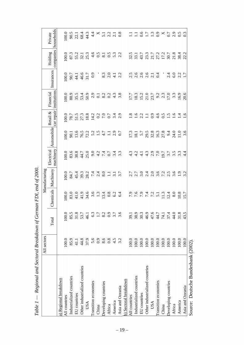
Table 1 gives some aggregated descriptive statistics for our dependent variable for the mostrecent year (2000). The data are sliced both according to the geographical distribution ofGerman firms’ FDI (Panel a) and the sectoral structure (Panel b). The Table shows, first of all,the dominance of German firms’ FDI held in other industrialized countries, which account fora share of 79-90% of all foreign direct investments. This distribution is also relativelyconsistent across sectors.

Perhaps somewhat surprisingly, the share of the EU countries in all industrialized countries isonly about one half, and it is sometimes even smaller than the share of the United States. Theimportance of the U.S. relative to intra-European FDI is particularly striking for theautomobiles sector (72 versus 14%) and the financial services sector (51 versus 36%). Formost other sectors, the U.S. is of smaller importance as a destination of FDI than Europe.2

Panel b of Table 1 shows the importance of each sector by region. For most regions covered,manufacturing accounts for around 40% of total FDI. The exception is China, where themanufacturing sector has a share of 74% of the total, which clearly exceeds the average forother emerging markets. Within the manufacturing sector, automobiles are the most importantsector, accounting for almost one half of the total. Interestingly, this sector has a below-average share of less than 6% of its FDI in EU countries. Table 1 also reveals a short-comingof the sectoral classification of our data: About one third of German firms’ FDI is classified asholding companies. Hence, these investments cannot be allocated to any specific sector withregard to the investing company.

2.2 Explanatory Variables

With regard to explanatory variables, our analysis is restricted mainly to macroeconomicdeterminants of FDI. (For similar approaches see Wheeler and Mody (1992), Barrell and Pain(1996), or Lipsey (1999).) While the reporting requirements of the Bundesbank are quiteencompassing with regard to the specifics of the foreign affiliate, little information is providedon the reporting firm itself. Essentially, the information on the reporting firm is restricted tothe sector in which it is active. Moreover, most of the information that we have on the foreignaffiliates is highly correlated with our dependent variable.

2 FDI of private households is an exception. However, this sector accounts for only 1% of German FDI.

– 4 –

Generally, FDI can be expected to respond to variables such as market size and marketdevelopment, geographical, cultural and economic distance between countries, the degree ofmacroeconomic stability, and the degree of regulations of countries. We capture these factorsas follows:

(i) Market size and development:

- Gross Domestic Product (GDP) controls for market size, and it is measured in currentUSD. GDP data have been obtained from the 2002 CD-rom Global DevelopmentIndicators of the World Bank. We expect this variable to influence positively GermanFDI outward stocks.

- Income dummies are included to control for the state of development of the host country.Low-income countries are defined as those with a per-capita GDP below 760 USD,lower-middle income countries as those with a per-capita GDP between 761 and 3000USD, upper-middle income countries: 3001-9300 USD, and high income countries asthose with a per-capita GDP above 9300 USD. Since these groups do not overlap, weexclude the low income dummy in the regression. All coefficients must therefore beinterpreted as effect relative to the benchmark of the group of countries with a per-capitaGDP below 760 USD.

- Bilateral trade is included as an alternative measure for the size of the foreign market.One problem with including trade as a regressor in a gravity equation explaining FDI isthe potential multicollinearity between trade and the remaining explanatory variables.Hence, we use the residual of a regression of trade on a border dummy, log distance, anEU dummy, log GDP, and log risk instead.3 The expected coefficient is positive(negative) if FDI and trade are complements (substitutes). Both effects are conceivablefrom a theoretical point of view. Brainard (1993) and Markusen and Venables (1998)argue that trade and FDI are substitutes. Conditions under which trade and FDI arecomplements are discussed in Helpman (1984) and Kleinert (2003). The bilateral tradedata have been obtained from the Deutsche Bundesbank in D-mark or euro (after 1999)and have been converted into USD.

3 We also instrumented trade through lagged foreign trade to account for its potential endogeneity. Resultswere qualitatively unchanged.

– 5 –

(ii) Geographic, cultural, and economic distance:

- Greater distance as measured by geographical distance in km is expected to lead tolower stocks of FDI abroad. Larger distance could be an impediment to FDI because itleads to higher communication and information costs and restricts face-to-facecommunication and networking. Moreover, a greater distance also reflects differences inculture, language, and institutions, which is also likely to decrease FDI.4

- Tariffs are average tariff rates taken from the World Bank.5 High tariffs increase thecosts of bilateral trade and may thus make FDI as a mode of entry into a foreign marketrelatively more attractive if exports and production abroad are substitutes. Hence, wewould expect a positive relationship between tariffs and FDI if trade and FDI aresubstitutes. If, in contrast, trade and FDI are complements, the expected impact of tariffson FDI would be negative.

- The presence of a common border is included as one proxy for distance costs. Theexpected coefficient of this 0/1-dummy is positive since foreign activities are generallyhigher in neighboring countries to which economic, political, cultural and personalrelations are much more intense.

- A 0/1-dummy for countries in which German is an official language is likewiseexpected to have a positive impact on FDI since speaking a common language easescommunication and also captures cultural similarity in a broader sense.

- We also include a 0/1-dummy variable EU which is set equal to one for countries thatare members of the European Union. The expected sign is positive, since the creation ofa Single Market should have promoted cross-border entry.

(iii) Stability and regulations:

- Risk as a composite index of country risk, is the political risk index taken from variousissues of Euromoney. It is defined as the risk of non-payment or non-servicing payments

4 The data have been taken from http://www.wcrl.ars.usda.gov/cec/java/capitals.htm. Distances are calculatedwith the following formula where lat i and long iare respectively latitude and longitude of Berlin and lat j andlong j those of the main economic center of country j (usually its capital).dist = 6370 * ARCOS( COS ( lat j / 57.2958) * COS ( lat i / 57.2958) * COS ( MIN ( 360 - ABS ( long j -long i) , ABS ( long j - long i ) ) / 57.2958) + SIN ( lat j / 57.2958 ) * SIN ( lat i / 57.2958 ) )

5 These data can be obtained from: http://www1.worldbank.org/wbiep/trade/data/TR_Data.html

– 6 –

for goods or services, loans, trade-related finance and dividends and the non-repatriationof capital. This variable takes values from 10 (no risk of non-payment) to 0 (norepayment expected). This risk index has a higher score when country risk is small.Since lower risk should encourage FDI, the expected coefficient is positive.

- Freedom is an index running from 1 through 7, whereby a value of 1 indicates thehighest degree of political freedom and liberty. The data have been obtained fromFreedom House (www.freedomhouse.org). As companies are expected to be drawn tocountries with a more liberal environment, we expect to find a negative link betweenfreedom and FDI.

- Two variables are included to capture the severity of regulations on cross-border capitalflows. Capital control is a 0/1-dummy, which is set equal to one if countries imposecontrols on cross-border financial credits. In addition, we control for the presence ofregimes of multiple exchange rates. Both dummy variables are expected to enter with anegative sign. The data are based on the IMF’s Annual Survey of Exchange RateRestrictions. Data prior to 1996 have kindly been provided by Gian-Maria Milesi-Ferretti, data after 1996 have been obtained from the IMF publications.

3 Empirical Results

We use different empirical models to analyze the determinants of German firms’ foreigndirect investment abroad. In a first step, we estimate quasi-panel regressions using data whichhave been sectorally aggregated across all firms being active in a given host country in a givenyear. In a second step, we study the sectoral dimension of the data estimating these quasi-panels separately for each sector. Hence, we are able to analyze whether determinants of FDIdiffer across sectors. Finally, we use micro-data. In addition, we use the number of Germanfirms that are active in a given country as the dependent variable in order to explain possibledifferences in the determinants of aggregated FDI, on the one hand, and the size of foreignaffiliates, on the other hand.

3.1 What Determines German FDI?

This section presents new evidence from gravity equations for the stocks of foreign directinvestments of German firms. Using data that have been aggregated across individual firmsfor each year, host country, and sector, we estimate a quasi-panel of the following form:

( ) ( ) ( ) ( ) ijtjtjjtijt variablescontroldistGDPFDI εββββ ++++= 3210 logloglog (1)

– 7 –

where subscripts i, j and t denote the sector, the host country, and the year respectively. Timefixed effects are included to capture possible trends. We also include a set of sectoral fixedeffects. The dependent variable (FDI) as well as GDP, GDP per capita, distance and risk areentered in logs6. Hence, the resulting coefficients can be interpreted as elasticities. Beforeestimating a full-fledged panel model, we use a quasi-panel, because in standard fixed effectsmodels, the impact of time invariant variables such as distance cannot be measured.

In addition to quasi-panel OLS results, we also present a fixed effects panel estimation whichaccounts for the clustered structure of the data. The cluster option implemented in STATAallows controlling for heteroscedasticity and autocorrelation of the residuals while exploitingthe panel dimension of our data. It computes a robust variance estimator based on a specificcluster structure and a calculated covariance matrix. The routine produces an estimator forclustered data (data are assumed not to be independent within groups, but independent acrossgroups). The resulting coefficients of the regression are unbiased.

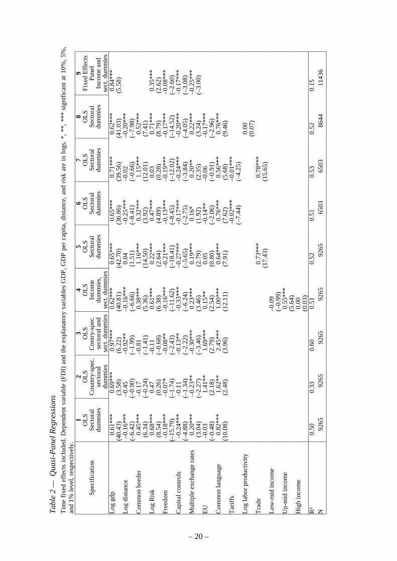
Table 2 presents results for the entire dataset, using eight different OLS specifications. Wevary the set of explanatory variables that we include. In all specifications with the exceptionof specification 2, we include sectoral dummies. In the second and third column, we reportregressions that include country-specific sectoral dummy variables. In the fourth and in thefixed effects specification (column 9), we include dummies for low-to-middle, middle-income, and high-income countries. Cut-off values for the income levels have been takenfrom the World Bank’s Global Development Indicators database. In columns 5 and 7, thetrade residual is included to control for the size of the foreign market. We use the residual of aregression of trade on the other exogenous variables to avoid the problem of multicollinearity.Columns 6 and 7 include a tariff variable as additional variable measuring economic distanceof the foreign market for German companies. Due to missing observations for the tariffvariable, however, our sample size drops to two-thirds for this specification. Column 8 givesthe results of a regression in which we control for labor productivity.7 The last specificationshows the results of a fixed effects regression which takes the panel dimension of our datasetinto account.

6 We believe that the effect of distance on FDI is better modeled by constant eleasticities given by thelogarithmic form than by a constant change of FDI in Euro per km as implied by a linear regression in levels.The logarithmic form implies a decreasing effect of an additional km on FDI measured in Euro. That mightstem from fixed costs. Moreover, the logarithmic form fits the data better.

7 We compute labor productivity as annual turn-over (pk04), converted into real USD, over the number ofemployees (pk05) in the given sector.

– 8 –

There are a couple of results which are fairly robust across different specifications. GDP ispositive and significant with an elasticity of around 0.7. As usual in gravity equations, GDP asproxy for the size of the foreign market has a significant positive effect on German FDI.

The proxies for risk, regulations, economic and cultural distance mostly have the expectedsigns and are also significant: a common border and a common language increase FDI, lowcountry risk and a high degree of freedom increase FDI (note that the two variables aredefined in an opposite way), and capital controls discourage FDI. The EU dummy, forinstance, is positive and significant. It is only for one variable that we find insignificantcoefficients or unexpected signs: Regimes of multiple exchange rates seem to encouragerather than deter foreign direct investment. One explanation would be that FDI is used as ameans to overcome barriers that multiple exchange rate regimes create.

Trade has, on average, a positive effect of German FDI in foreign countries. The coefficient islarge and significant. A 10% increase in bilateral trade increases the FDI stock of Germancompanies by about 7.5%. The specifications suggests a positive (i.e. complementary)relationship between (aggregated) trade and FDI. The result is also robust with regard to theuse of foreign sales (not reported) as the dependent variable. The complementary relationshipis also supported by the negative coefficient we obtain for the impact of tariffs on FDI.

Generally, our RHS variables are able to explain a little over 50% percent of the variation ofGerman foreign direct investment stocks across countries. The explanatory power dropsconsiderably though if sectoral dummies are not included. In this case, the adjusted R² doesreach a value of only 0.33. This can be taken as a first indication that sectoral differencesmatter. Results are relatively insensitive, in contrast, with regard to including dummies forcountries from different income groups.

With regard to the effect of distance on German FDI, we obtain a statistically andeconomically significant coefficient of –0.2 to –0.35, depending on the specification chosen.These estimates are somewhat at the lower bound of the findings of the earlier literature onforeign trade. (Frankel (1997) and Leamer and Levinsohn (1995) review the literature ongravity-type equations for foreign trade which finds a coefficient of around –0.6.) Our resultsindicate that FDI declines by about 25% if distance doubles. The negative effect of distanceon German FDI in foreign countries is completely picked up by the trade variable if trade isincluded (Column 7).

– 9 –

3.2 Do Determinants of FDI Differ Across Sectors?

The results of Table 2 point to sectoral differences in the data since the sectoral dummies thatwe have included are typically significant. Hence, one obvious question to ask is whether theeffect of some of the exogenous variables of interest, notably of the distance coefficient,differs among sectors. In other words, we are interested in the question to what extentaggregation over the different sectors might be influencing our results.

Essentially, our sample contains information on almost 30 economic sectors, coveringmanufacturing, services, and agriculture. However, for some of these sectors, sample sizes arerelatively small if, in addition, we are interested in the regional and the time pattern of theirinternational expansion. Therefore, rather than estimating individual cross-section regressionsat a sectoral level, this section looks at quasi-panel estimates for the entire time period.

Results for the entire sample are reported in Table 3. We present results for the largest12 sectors. In addition to the results reported here, we have tested the robustness of theseresults also by including interaction terms between distance and the time dummies and byincluding tariffs and a proxy for labor productivity. Generally, results were fairly insensitive tothese changes.

The sectoral results show, first of all, that there is quite some heterogeneity in thedeterminants of FDI at a sectoral level. Market size (GDP), for instance, has a relatively largeimpact on the chemicals industry, the automobiles industry, machinery, and the informationtechnology sector (elasticity of around 0.90 with respect to GDP). The high costs of setting upa foreign affiliate in those sectors can explain this high elasticity. For other sectors such asfinancial services, construction, or textiles, the coefficient on GDP is only about half that size.

Sectors also seem to differ in their sensitivity to regulations and cultural proxies. It is difficult,however, to trace a clear pattern in the data since many coefficients become insignificant oreven switch signs as we run different specifications of our baseline model. Interestingly, theEU dummy is often significant and also carries a positive sign, suggesting that the SingleMarket Program has stimulated German FDI. The only exception is the construction sector,where the EU dummy has a negative impact.

It is interesting to note that the impact of distance differs quite significantly among sectors.Graph 1 plots the distance coefficients we obtain for 25 sectors for which we had a reasonablenumber of observations. The number of observations varies considerably across sectors, henceresults should be taken as being indicative of trends rather than being precise point estimates.

– 10 –

A couple of results are interesting. On average, the marginal effect of distance for the wholesample is around –0.3. Distance has a negative impact on German FDI in most sectors. It hasan above-average importance (in absolute terms) for the electricity sector, glass and ceramics,plastic products, retail trade, manufacturing of coke and refined petroleum products, and paperproducts. However, multinationals in the chemicals industry and hotels and restaurant areparticularly attracted to distant markets. Finally, there is a group of sectors for which distancedoes not seem to be important (e.g. construction, financial services, information technology,housing, wood processing, agriculture).

3.3 What Determines the Size of Foreign Affiliates?

Finally, we explicitly use the microstructure of the database. Although we lack information onthe balance sheets and income statements of the reporting firms, this exercise can provide uswith additional information on the determinants of FDI. Results are reported in Table 4.Technically, we estimate equation (2) but the dependent variable is not aggregated acrosssectors but rather captures each individual investment into a foreign affiliate.8 We indirectlyaccount for the size of the reporting company by including the number of its foreign affiliatesworldwide as an explanatory variable. This variable size is always positive and significant(Table 4, panel b), which implies that companies that maintain more foreign affiliates alsohave foreign affiliates which are of above-average size.

Table 4 reports two sets of regressions. In a first specification (panel a), we regress the size ofthe foreign affiliate on the set of regressors used above. In a second specification (panel b), weadditionally include the number of foreign affiliates of the reporting company to control forfirm size, and we include aggregated trade between Germany and the recipient country. In allregressions, we include sectoral dummies as well as dummies for the income level of therecipient country. In addition, we have run a number of robustness checks (results notreported), on which we will comment below. We run the two different specificationspresented in Table 4 for each of the years 1990-2000 individually. This allows studyingchanges in the determinants of FDI over time. The main reason why we do not estimate a full-fledged panel model is that the codes of the companies have been changed in 1996. Hence, wecannot trace a particular reporting company through the 10 years under study. The number offoreign affiliates on which we have information has doubled during the observation periodfrom 10,847 entries for the year 1990 to 21,285 entries for the year 2000.

8 We equate the size of the foreign affiliate with the share in equity capital hold by one German company. Theinterpretation of our results might be biased if German companies hold smaller shares of total equity in thoseforeign affiliates which are located in nearby markets.

– 11 –

Running the same regressions for the micro-data as those presented in Section 3.2 for thesectorally aggregated data gives a much poorer statistical fit. In terms of explanatory power,our regressions explain at most 16% of the cross-country variation in the size of firms' foreigndirect investment. The main reason is that we have generally not included any firm-specificexplanatory variables. The adjusted R² even increases to over 30% if we additionally includeinteraction terms between the explanatory variables and a dummy for the size of the Germanmultinational company (results not reported). For this purpose, small multinational companieshave been defined as companies which total number of affiliates is smaller than three.

When comparing the results for the regressions using micro-data to those using aggregateddata (i.e. comparing Tables 2 and 4), there is only one variable for which we obtain a resultwhich is robust across specifications: GDP has a positive and significant impact on FDI acrossthe different specifications that we use.

For some variables, we do obtain results that are similar across specifications although thepicture is more mixed. For these variables, we also obtained quite a few insignificantcoefficient estimates. Risk and freedom, for instance, tend to have a positive and negativeimpact on the size of foreign affiliates, respectively. Also, the dummies for current and capitalaccount restrictions have relatively consistent signs, i.e. the presence of capital controlslowers FDI while the presence of multiple exchange rates increases FDI. While, if significant,the common language dummy is positive, it is significant in only a few of the specifications.The EU dummy tends to be negative in contrast, suggesting that relatively small affiliates areset up in these countries.

The variable for which we obtain the largest differences between the quasi-panel regressions(Table 2) and the regressions using the micro-data (Table 4, Panel a) is the distance variable.While we obtain a statistically significant negative link between distance and FDI for theaggregated data, the effect of distance is often positive for the micro-data. Our second proxyfor proximity, the common border dummy, also has a different effect. In contrast to theaggregated equations (Table 2), where we generally obtain a positive effect, we often obtain anegative sign in the micro-data regressions (Table 4).

The positive effect of distance even survives in some cases if we additionally control for thelevel of total foreign trade between Germany and the recipient country (Table 4, Panel b). Atthe same time, the effect of trade is negative and not, as for the aggregated data, positive. Thisresult could partly be seen as a mirror-image of the different results obtained for distance.Since gravity models for trade overwhelmingly find that aggregated trade and distance arenegative correlated, a negative link between a given variable and trade should be associatedwith a positive link between this variable and distance. The negative border effect remains

– 12 –

even if we control for the level of foreign trade. The interpretation of this result is that it is thesmaller foreign affiliates which are set up in neighboring countries, as has also been suggestedby the negative EU dummy.

Since, for most other variables, we obtain results that are relatively consistent in sign whencomparing regressions for aggregated and disaggregated data, the differential effect of tradeand “proximity” obviously warrants an explanation. Two explanations, which are notmutually exclusive, are conceivable:

The first explanation for the negative link between trade and the size of foreign affiliates isthat, in countries with which Germany conducts a lot of foreign trade, the average size of theforeign affiliate is smaller. One interpretation would be that these affiliates are set up tofacilitate trade and not as foreign production units. Even if they are production units, the shareof imported inputs might be higher than in affiliates which are far away from Germany. Thus,the value added in these affiliates might be low, which requires less capital. To explore thisrelationship is beyond the scope of this paper but an interesting task for further research.

The second explanation for the positive link between distance and the size of foreign affiliatesis that firms set up smaller foreign affiliates on average in nearby countries, because it isprofitable to do so even for smaller units. Set-up costs of establishments in remote countries,in contrast might be too high for small affiliates. If this explanation was correct, then thenegative effect of distance on FDI found in aggregated data must be due to a decline in thenumber of affiliates as distance increases which overcompensates the size effect of theaverage single affiliate.

We test whether this explanation is confirmed by the data by running regressions, using thenumber of German firms' foreign affiliates as the dependent variable. Results are reported inTables 5a and 5b. These results are consistent with the hypothesis that proximity (measuredthrough the presence of a common border or through distance) has a different effect on thesize of the foreign affiliate than on the number of firms abroad. As for the aggregated data, thenumber of firms is relative negatively (positively) to distance (common border). The mirror-image of this finding is that the effect of trade differs. Hence, nearby countries, with whichGermany conducts a lot of trade, attract many small foreign affiliates whereby remotecountries, with which Germany conducts little foreign trade, attract few large foreignaffiliates. Since the impact of proximity and trade on the number of foreign affiliatesdominates, we obtain the aggregated effect of a negative (positive) link between total FDI anddistance (trade).

– 13 –

Graph 2 shows descriptive statistics which confirm that affiliates located in bordering andnearby countries are smaller on average than affiliates located in more remote countries.Graph 2 shows the means of employment, sales, and FDI of affiliates in bordering countriesover time. Overall, affiliates in bordering countries are smaller in terms of employment, sales,and the sum of equity capital invested than affiliates in more remote regions. Thesedifferences have remained relatively stable over time. While all affiliates have grown in thepast ten years on average, the gap between the size of affiliates in the two regions consideredhas remained almost unchanged.

The regression analysis reported above has also shown that smaller foreign affiliates are set upin countries with which Germany conducts a lot of foreign trade. This results can beinterpreted as smaller affiliates being used for distribution rather than production. Since ourdataset provides us with information on the sector of the foreign affiliate, we can checkwhether this hypothesis is confirmed by the data. Table 6 shows differences in the importanceof wholesale trade for firms of different size in terms of employment and in different regions.The most important individual sector of the foreign affiliates is wholesale trade, whichaccounts for more than one third of all foreign establishments of German firms.

With regard to the importance of wholesale trade activity, the size of employment in theforeign affiliates matters most. Whereas wholesale trade is the main line of business for 36%of the firms in the sample, it accounts for 43% of the activities of affiliates with less than 50employees and only 18% for those with more than 50 employees. This difference also remainsif we break up the sample into bordering and nearby countries, on the one hand, and moredistant countries, on the other hand. Hence, less employees are needed ceteris paribus inaffiliates being engaged in distribution as opposed to production abroad. Breaking up thesample into reporting companies that have only 1 or 2 foreign affiliates and those that havemore than 2 foreign affiliates shows that wholesale trade and thus distribution is somewhatmore important for those having more affiliates abroad. Looking at differences betweennearby and remote countries also shows that wholesale trade is somewhat more important inthe nearby regions.

4 Avenues for Future Research

This paper has provided a first assessment of the determinants of German firms’ foreign directinvestment activities, using a comprehensive firm-level dataset. We have looked at the data atdifferent levels of aggregation. In a first step, we have aggregated the data by country andsector. In a second step, we have focused the analysis on the sectoral differences in thedeterminants of FDI. In a final step, we have used the size of foreign affiliates and thus firm-level data as the dependent variable.

– 14 –

Interestingly, there are only two results which are fairly robust against changes in thespecification. As shown by the positive impact of GDP and the negative impact of risk onFDI, German firms are drawn to large and safe markets. Other traditional determinants of FDIhave more heterogenous effects, and their impact differs according to the sector and the sizeof the foreign affiliate under study.

One interesting result of this study has been that regional and cultural proximity have adifferential effect on the size of the foreign affiliate and the number of firms being present in agiven host country. More specifically, many small affiliates tend to be set up in nearbymarkets whereas few but, on average, larger affiliates tend to be set up in distant markets. Thisis shown by the negative (positive) link that we find between the border dummy (distance) andthe size of the foreign affiliate. Opposite effects of these variables are found for the totalnumber of affiliates. For aggregate FDI, the effect of proximity on the number of firmsdominates. Hence, we find that there is more FDI in geographically close countries withwhich Germany shares a common border.

Different effects of distance on the number and the size of foreign affiliates are a mirror-imageof the differential effect of aggregated bilateral trade on these two measures of German firms’FDI. Whereas there is a positive link between aggregated FDI (and the number of Germanaffiliates in a given market) and trade, the link is negative for the size of the affiliate. Oneinterpretation of this result is that affiliates which are production units and therefore substitutetrade are larger in size. An affiliate set up for distribution can be smaller (with regard to theequity investment it requires) than a production unit.

This interpretation of the link between trade and FDI also shows one potentially interestingdirection for future research. It would be of interest to test in more detail to what extentforeign affiliates are set up to facilitate trade or production abroad. The sector classificationsof the foreign affiliate and the parent company might help to distinguish sales units fromproduction units. Another way of discriminating between the two purposes might be tocompare equity-sales-ratios or employment-sales-ratios for the affiliates. In general, salesunits show lower ratios than production units.

A second extension of this work would be to try and explain the differences in thedeterminants of FDI for different sectors. Controlling for sector-specific factors such as thedegree of competition, the intensity of regulations, or the relative importance of fixed versusvariable costs of entry would be one step into this direction.

Finally, it would be of interest to shed more light on the question to what extent FDI and othermodes of integration are linked. Results of this study suggest that aggregated FDI and trade

– 15 –

are complements. In addition, it would be of interest to analyze links between FDI and otherfactors flows. For instance, business services, as an important intermediary input in affiliates’production might be interesting to analyze. A study on the relationship of business servicesand FDI can shed light on the choice between licensing and FDI, because intra-firminformation flows are one likely candidate for the internalization decision of MNEs.

Our results also hold some interesting implications for future theoretical work on thedeterminants of FDI. Typically, theoretical models assume the existence of firms that do notdiffer in size. This helps to derive implications on aggregate FDI on the basis of the analysisof a representative firm. This approach has the disadvantage, however, that differences in thesize of affiliates cannot be analyzed. The number of affiliates, in turn, is endogenous in thesemodels and depends only on the size of the country. However, our results show that theseassumptions may not reflect reality sufficiently. Rather, proximity seems to have an impactboth on the size of the affiliate and on the number of affiliates being set up abroad. Proximitymay have differential effects on aggregate FDI. Moreover, modeling differences in the foreigninvestment behavior of different sectors seems promising (see, e.g., Helpman et al. (2003) fora recent contribution). All this is left to future research.

– 16 –

References

Andersson, T., and T. Fredriksson (2000). Distinction Between Intermediate and FinishedProducts in Intra-Firm Trade. International Journal of Industrial Organization 18: 773–792.

Barrell, R., and Pain N. (1996). An Econometric Analysis of US Foreign Direct Investment.Review of Economics and Statistics 78: 200–207.

Brainard, S.L. (1993). A Simple Theory of Multinational Corporations and Trade with aTrade-off between Proximity and Concentration. NBER Working Paper 4269. NationalBureau of Economic Research, Cambridge, Mass.

Buch, C.M. (2002). Distance and International Banking. Kiel Institute for World Economics.Mimeo.

Carr, D.L., J.R. Markusen, and K.E. Maskus (2001). Estimating the Knowledge CapitalModel of the Mulitinational Enterprise. American Economic Review 91 (3): 693–708.

Deutsche Bundesbank (2002). Kapitalverflechtungen mit dem Ausland. StatistischeSonderveröffentlichung 10. Frankfurt a.M.

Dunning, J. (1977). Trade, location of economic activities and the MNE: A search for aneclectic approach. In P.-O. Hesselborn, B. Phlin and P.-M. Wijkman (eds.), TheInternational Allocation of Economic Activity. London: MacMillan. 395-418.

Egger, Peter (2003). On the Problem of Endogenous Unobserved Effects in the Estimation ofGravity Models, Journal of Economic Integration (forthcoming).

Frankel, J. (1997). Regional Trading Blocks. Institut for International Economics. WashingtonD.C.

Head, K., and J. Ries (2001). Overseas Investment and Firm Exports. Review of InternationalEconomics 9 (1): 108–122.

Helpman, E. (1984). A Simple Theory of International Trade with Multinational Corporations.Journal of Political Economy 92 (3): 451–471.

Helpman, E., M.J. Melitz, and S.R. Yeaple (2003). Export versus FDI. National Bureau ofEconomic Research (NBER). Working Paper 9439. Cambridge, MA.

– 17 –

Horstmann, I. and J. Markusen (1992). Endogenous Market Structures in International Trade(Natura Facit Saltum). Journal of International Economics 32 (1/2): 109–129.

Kleinert, J. (2001). The Time Pattern of the Internationalisation of Production. GermanEconomic Review 2 (1): 79–98.

Kleinert J. (2003). Growing Trade in Intermediate Goods: Outsourcing, Global Sourcing orIncreasing Networks of Multinational Enterprises? Review of International Economics.(forthcoming).

Leamer, E.E., and J. Levinsohn (1995). International Trade Theory: The Evidence. In: Grossman, G.,and K. Rogoff (eds.). Handbook of International Economics. Vol. III. Elsevier: 1339–1394.

Lipponer, A. (2002a). A „new“ microdatabase for German FDI. Paper presented at theBundesbank Spring Conference. May 2002. mimeo.

Lipponer, A. (2002b). Mikrodatenbank Direktinvestitionsbestände: Handbuch. DeutscheBundesbank. Frankfurt a. M. mimeo.

Lipsey, R.E (1999). The Location and Characteristics of US Affiliate in Asia. NBER WorkingPaper 6876. Cambridge, MA.

Markusen, J. (1995). The Boundaries of Multinational Enterprises and the Theory ofInternational Trade. Journal of Economic Perpectives 9 (2): 169–189.

Markusen, J. and A. Venables (2000). The Theory of Endowment, Intra-Industry, andMultinational Trade, Journal of International Economics 52 (2): 209–234.

Markusen, J. and A. Venables, (1998). Multinational Firms and the New Trade Theory.Journal of International Economics 46 (2): 183–203.

Raff, H. and K. Srinivasan (1998). Tax Incentives for Import-Substituting Foreign Investment:Does Signaling Play a Role? Journal of Public Economics 67: 167–193.

Raff, H. and Y.H. Kim (1999). Optimal Export Policy in the Presence of Informational Barriersto Entry and Imperfect Competition. Journal of International Economics 49: 99–123.

Wheeler, D. and A. Mody (1992). International Investment Location Decisions: the Case ofU.S. Firms. Journal of International Economics 33: 57–76.

– 18 –

Tabl

e 1

— R

egio

nal a

nd S

ecto

ral B

reak

dow

n of

Ger

man

FD

I, en

d of

200

0.A

ll se

ctor

sM

anuf

actu

ring

Tota

lC

hem

ical

sM

achi

nery

Elec

trica

lm

achi

nery

Aut

omob

ileR

etai

l &ca

r rep

air

Fina

ncia

lin

stitu

tions

Insu

ranc

esH

oldi

ngco

mpa

nies

Priv

ate

hous

ehol

dsa)

Reg

iona

l bre

akdo

wn

All

coun

tries

100.

010

0.0

100.

010

0.0

100.

010

0.0

100.

010

0.0

100.

010

0.0

100.

0In

dust

rializ

ed c

ount

ries

85.9

85.5

83.0

84.7

83.6

90.1

78.7

88.9

90.7

87.3

90.5

EU c

ount

ries

41.1

31.8

41.0

45.4

38.8

13.6

51.5

35.5

44.1

55.2

22.1

Oth

er in

dust

rializ

ed c

ount

ries

44.8

53.7

41.9

39.3

44.7

76.5

27.3

53.4

46.6

32.1

68.4

USA

37.9

46.1

34.6

28.2

25.0

72.2

18.8

50.9

31.7

25.3

44.3

Tran

sitio

n ec

onom

ies

5.6

6.3

3.6

7.4

9.0

5.2

14.2

2.

9 0.

9 4.

6 4.

4C

hina

0.9

1.7

1.3

2.4

4.2

1.5

0.2

0.1

-0.

5X

Dev

elop

ing

coun

tries

8.6

8.2

13.4

8.0

7.4

4.7

7.0

8.2

8.3

8.1

5.1

Afr

ica

0.8

0.9

0.8

1.1

0.7

1.1

0.7

0.2

2.0

0.5

2.2

Am

eric

a4.

53.

76.

23.

13.

42.

93.

44.

34.

15.

32.

1A

sia

and

Oze

ania

3.2

3.6

6.4

3.7

3.3

0.7

2.9

3.8

2.2

2.2

0.8

b) S

ecto

ral b

reak

dow

nA

ll co

untri

es10

0.0

39.1

7.9

2.7

4.3

17.3

1.8

17.7

2.5

32.5

1.1

Indu

stria

lized

cou

ntrie

s10

0.0

38.9

7.6

2.7

4.2

18.1

1.6

18.3

2.6

33.1

1.1

EU c

ount

ries

100.

030

.37.

93.

04.

15.

72.

215

.22.

643

.70.

6O

ther

indu

stria

lized

cou

ntrie

s10

0.0

46.9

7.4

2.4

4.3

29.5

1.1

21.0

2.6

23.3

1.7

USA

100.

047

.67.

22.

02.

932

.80.

923

.72.

121

.71.

3Tr

ansi

tion

econ

omie

s10

0.0

44.7

5.1

3.6

7.0

16.3

4.6

9.2

0.4

27.2

0.9

Chi

na10

0.0

74.1

11.3

7.2

19.7

27.8

0.5

2.3

-17

.2X

Dev

elop

ing

coun

tries

100.

037

.412

.42.

53.

79.

41.

517

.02.

430

.70.

7A

fric

a10

0.0

44.0

8.0

3.6

3.5

24.0

1.6

3.3

6.0

21.8

2.9

Am

eric

a10

0.0

31.8

10.8

1.9

3.3

11.0

1.4

16.9

2.2

38.4

0.5

Asi

a an

d O

zean

ia10

0.0

43.5

15.7

3.2

4.4

3.6

1.6

20.6

1.7

22.2

0.3

Sour

ce:

Deu

tsch

e B

unde

sban

k (2

002)

.

– 19 –

Tabl

e 2

— Q

uasi

-Pan

el R

egre

ssio

nsTi

me

fixed

effe

cts

incl

uded

. Dep

ende

nt v

aria

ble

(FD

I) a

nd th

e ex

plan

ator

y va

riabl

es G

DP,

GD

P pe

r cap

ita, d

ista

nce,

and

risk

are

in lo

gs. *

, **,

***

sig

nific

ant a

t 10%

, 5%

,an

d 1%

leve

l, re

spec

tivel

y.

Spec

ifica

tion

1 O

LS Se

ctor

aldu

mm

ies

2O

LSC

ount

ry-s

pec.

sect

oral

dum

mie

s

3 O

LSC

ontr y

-spe

c. se

ctor

al a

ndse

ct. d

umm

ies

4 O

LS In

com

edu

mm

ies,

sect

. dum

mie

s

5 O

LS Se

ctor

aldu

mm

ies

6 O

LS Se

ctor

aldu

mm

ies

7 O

LS Se

ctor

aldu

mm

ies

8 O

LS Se

ctor

aldu

mm

ies

9 Fi

xed

Effe

cts

Pane

l In

com

e an

dse

ct. d

umm

ies

Log

gdp

0.61

***

(40.

43)

0.69

***

(3.5

8)0.

97**

*(6

.22)

0.62

***

(40.

81)

0.65

***

(42.

70)

0.65

***

(36.

86)

0.71

***

(39.

56)

0.62

***

(41.

03)

0.84

***

(5.5

8)Lo

g di

stan

ce–0

.16*

**(–

6.42

)–0

.45

(–0.

90)

–0.9

2**

(–1.

99)

–0.1

6***

(–6.

66)

0.04

(1.5

1)–0

.25*

**(–

8.41

)–0

.02

(–0.

66)

–0.2

0***

(–7.

98)

Com

mon

bor

der

0.45

***

(6.3

4)–0

.17

(–0.

24)

–0.8

1(–

1.41

)0.

38**

*(5

.36)

1.16

***

(14.

50)

0.32

***

(3.9

2)1.

15**

* (1

2.01

)0.

52**

* (7

.41)

Log

Ris

k0.

68**

*(8

.54)

0.47

(0.2

6)–0

.11

(–0.

68)

0.61

***

(6.3

8)0.

22**

*(2

.64)

0.47

***

(4.8

9)0.

03 (0

.28)

0.71

***

(8.7

9)0.

35**

* (2

.62)

Free

dom

–0.1

8***

(–15

.79)

–0.0

7*(–

1.74

)–0

.08*

*(–

2.43

)–0

.16*

**(–

11.6

2)–0

.21*

**(–

18.4

1)–0

.13*

**(–

8.45

)–0

.19*

** (–

12.0

2)–0

.17*

** (–

14.5

2) –0

.08*

**(–

2.60

)C

apita

l con

trols

–0.2

4***

(–4.

88)

–0.1

1(–

1.34

)–0

.13*

*(–

2.22

)–0

.33*

**(–

6.24

)–0

.27*

**(–

5.65

)–0

.17*

**(–

2.75

)–0

.24*

** (–

3.84

)–0

.20*

** (–

4.05

)–0

.17*

**(–

3.08

)M

ultip

le e

xcha

nge

rate

s0.

20**

*(3

.04)

–0.2

3**

(–2.

27)

–0.3

0***

(–3.

46)

0.23

***

(3.4

6)0.

19**

*(2

.79)

0.16

*(1

.92)

0.20

** (2

.35)

0.22

***

(3.2

4) –0

.25*

**(–

3.00

)EU

–0.0

3(–

0.48

)1.

41**

(2.1

8)1.

69**

*(2

.79)

0.15

**(2

.54)

0.05

(0.8

0)–0

.14*

*(–

2.06

)–0

.06

(–0.

91)

–0.1

7***

(–2.

96)

Com

mon

lang

uage

0.82

***

(10.

08)

1.62

**(2

.48)

2.45

***

(3.9

6)1.

00**

*(1

2.11

)0.

64**

*(7

.91)

0.76

***

(7.6

2)0.

56**

* (5

.68)

0.76

***

(9.4

6)Ta

riffs

–0.0

2***

(–7.

44)

–0.0

1***

(–4.

25)

Log

labo

r pro

duct

ivity

0.00

(0.0

7)Tr

ade

0.73

***

(17.

43)

0.78

***

(15.

65)

Low

-mid

inco

me

–0.0

9 (–

0.99

)U

p-m

id in

com

e0.

55**

* (5

.64)

Hig

h in

com

e0.

00 (0

.03)

R²

0.50

0.33

0.60

0.51

0.52

0.51

0.53

0.52

0.15

N92

6592

6592

6592

6592

6565

0365

0386

4411

436

– 20 –

Tabl

e 3

— S

ecto

ral R

egre

ssio

ns

OLS

est

imat

es o

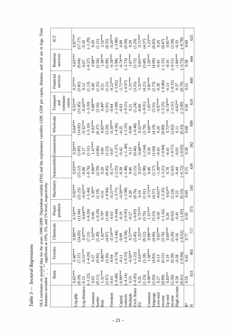
n po

oled

dat

a fo

r th

e ye

ars

1990

-200

0. D

epen

dent

var

iabl

e (F

DI)

and

the

expl

anat

ory

varia

bles

GD

P, G

DP

per

capi

ta, d

ista

nce,

and

ris

k ar

e in

logs

. Tim

edu

mm

ies i

nclu

ded.

* , **, **

* sign

ifica

nt a

t 10%

, 5%

, and

1%

leve

l, re

spec

tivel

y.

Ban

kTe

xtile

sC

hem

ical

sPl

astic

prod

ucts

Mac

hine

ryA

utom

obile

sCon

stru

ctio

nW

hole

sale

Tran

spor

tan

dco

mm

uni-

catio

n

Fina

ncia

lse

rvic

esB

usin

ess

serv

ices

ICT

Log

gdp

0.65

***

(9.2

9)0.

40**

*(7

.37)

0.99

***

(24.

05)

0.74

***

(11.

04)

0.95

***

(21.

23)

0.93

***

(15.

12)

0.50

***

(5.8

5)0.

64**

*(1

4.82

)0.

55**

*(1

1.85

)0.

37**

*(5

.81)

0.65

***

(9.6

4)0.

87**

*(1

7.17

)Lo

g di

stan

ce–0

.15

(–1.

22)

–0.3

1***

(–4.

20)

0.47

***

(7.1

1)–0

.64*

**(–

6.26

)–0

.42*

**(–

5.44

)–0

.08

(–0.

76)

0.17

(1.5

1)–0

.32*

**(–

5.16

)–0

.26*

**(–

3.10

)0.

12(1

.13)

–0.0

7(–

0.57

)–0

.10

(–1.

29)

Com

mon

bord

er0.

03(0

.11)

0.27

(0.9

5)1.

02**

*(5

.39)

–0.0

6(–

0.29

)0.

39**

(2.1

9)0.

80**

(2.5

9)1.

47**

*(4

.86)

0.93

***

(6.3

7)0.

88**

*(3

.56)

0.40

(1.3

1)0.

68**

(2.5

6)0.

20(1

.21)

Ris

k1.

31**

*(2

.67)

0.86

***

(3.2

6)1.

42**

*(4

.97)

0.70

*(1

.69)

–0.3

1(–

0.94

)0.

20(0

.45)

0.60

(1.2

3)0.

85**

*(3

.20)

0.49

*(1

.91)

0.51

(1.2

1)1.

39**

*(2

.90)

2.16

***

(6.5

5)Fr

eedo

m–0

.03

(–0.

48)

–0.0

4(–

0.74

)–0

.14*

**(–

3.44

)–0

.03

(–0.

44)

–0.2

1***

(–3.

71)

–0.1

7**

(–2.

25)

–0.0

7(–

1.37

)–0

.18*

**(–

4.56

)–0

.04

(–1.

09)

–0.2

2***

(–5.

02)

–0.3

4***

(–5.

98)

–0.2

0***

(–3.

86)

Cap

ital

cont

rols

–0.8

9***

(–4.

14)

–0.1

1(–

0.55

)–0

.09

(–0.

58)

–0.1

9(–

0.95

)–0

.50*

**(–

2.98

)–0

.39

(–1.

48)

–0.4

2(–

1..4

0)–0

.25

(–1.

55)

–0.0

3(–

0.21

)–1

.71*

**(–

6.07

)–0

.74*

**(–

2.73

)0.

09(0

.58)

Mul

tiple

Exch

. Rat

es0.

33(–

0.95

)–0

.50*

*(–

2.22

)0.

57**

*(3

.45)

–0.2

7(–

0.83

)0.

20(0

.76)

0.46

(1.1

5)0.

13(0

.46)

–0.0

8(–

0.48

)0.

21(1

.24)

1.31

***

(3.5

5)1.

07**

*(3

.72)

0.29

(1.2

9)EU

0.35

(1.2

3)0.

63**

*(3

.18)

1.35

***

(9.1

2)0.

75**

*(3

.76)

0.19

(1.0

1)0.

55**

(1.9

8)–0

.68*

**(–

2.64

)0.

55**

*(3

.70)

–0.0

0(–

0.01

)1.

31**

*(4

.21)

0.85

***

(3.4

0)0.

71**

*(4

.37)

Com

mon

lang

uage

0.90

***

(2.9

3)1.

38**

*(4

.83)

0.98

***

(4.0

6)1.

15**

*(5

.53)

0.73

***

(4.5

7)0.

48(1

.57)

0.50

(1.0

4)0.

60**

*(4

.19)

1.05

***

(3.5

5)0.

81**

*(2

.73)

1.20

***

(4.0

9)1.

23**

*(6

.83)

Low

-mid

inco

me

0.27

(0.8

9)0.

13(0

.31)

0.65

***

(3.7

6)–0

.50

(–1.

42)

–0.6

5**

(–2.

35)

–1.3

8***

(–3.

21)

–0.4

3(–

0.84

)0.

20(0

.89)

–0.9

7***

(–5.

25)

–0.3

0(–

0.80

)–0

.45

(–1.

55)

0.20

(0.6

7)U

p-m

idin

com

e0.

83**

(2.5

0)0.

19(0

.39)

0.69

***

(3.2

6)0.

20(0

.62)

0.63

**(2

.24)

0.78

(1.6

2)–0

.41

(–0.

71)

0.73

***

(2.6

2)–0

.74*

**(–

3.51

)–0

.13

(–0.

31)

–0.1

6(–

0.51

)0.

81**

(2.5

8)H

igh

inco

me

0.28

(0.6

1)–0

.58

(–0.

94)

–0.1

6(–

0.52

)–0

.41

(–1.

03)

0.22

(0.5

3)–0

.44

(–0.

72)

–0.0

3(–

0.05

)0.

11(0

.33)

–0.6

2**

(–2.

00)

0.37

(0.7

0)–1

.84*

**(–

3.75

)–0

.33

(–0.

78)

R²

0.55

0.42

0.77

0.59

0.69

0.55

0.38

0.68

0.50

0.55

0.58

0.69

N43

346

571

737

354

543

939

269

961

946

044

462

5

– 21 –

Graph 1 — Sectoral Distance CoefficientsThis graph plots the distance coefficients obtained from a baseline regression of the types reported in Table 3.Data were entered in logs, and time dummies are included. Insignificant coefficients are entered as zeros.

Electricity Glass, ceramics Plastic products

Retail Coke, refinery products Paper, paper products

Machinery Wholesale

Textiles Mining,quarrying

Transport, communication Holding companies

Bank ICT

Motor vehicles Business services

Wood, wood products Food

Financial services Metal

Agriculture Construction

Sewage, refuse disposal Hotels, restaurants

Chemicals 0 0.5 -0.5-1-1.5-2-2.5

– 22 –

Tabl

e 4

— R

egre

ssio

ns U

sing

Mic

ro-D

ata

OLS

est

imat

es. D

epen

dent

var

iabl

e (F

DI)

and

the

expl

anat

ory

varia

bles

GD

P, G

DP

per

capi

ta, d

ista

nce,

and

ris

k ar

e in

logs

. * , **, **

* sig

nific

ant a

t 10%

, 5%

, and

1%

leve

l,re

spec

tivel

y. W

hite

-het

eros

ceda

stic

ity ro

bust

sta

ndar

d er

rors

hav

e be

en u

sed.

In P

anel

(b) a

nd (c

) 'si

ze' i

s m

easu

red

as th

e to

tal n

umbe

r of f

orei

gn a

ffilia

tes

wor

ldw

ide

owne

dby

the

repo

rting

com

pany

, and

'tra

de' g

ives

the

aggr

egat

ed v

olum

e of

fore

ign

trade

(su

m o

f exp

orts

and

impo

rts d

ivid

ed b

y tw

o) b

etw

een

Ger

man

y an

d th

e ho

st c

ount

ry. I

npa

nel (

c), t

he sm

alle

st a

nd la

rges

t 10%

of t

he o

bser

vatio

ns h

ave

been

dro

pped

. Sec

tora

l dum

mie

s are

incl

uded

.

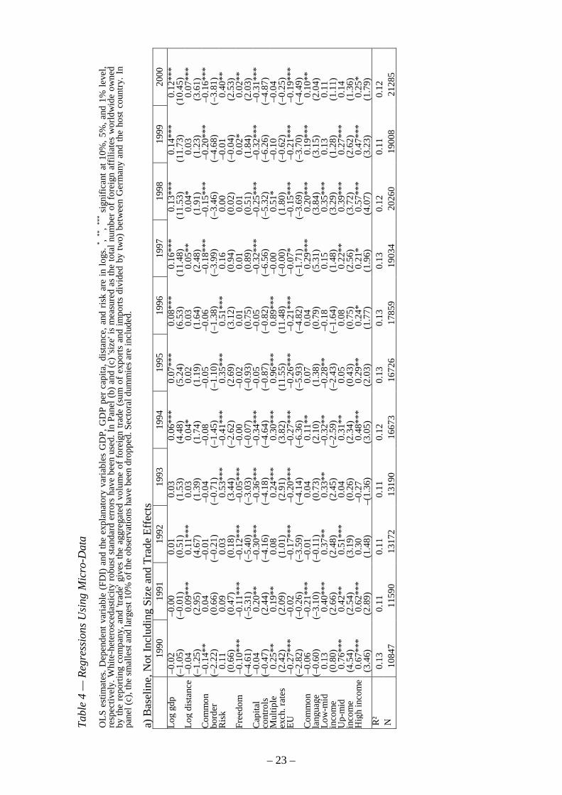
a) B

asel

ine,

Not

Incl

udin

g Si

ze a

nd T

rade

Eff

ects

1990

1991

1992

1993

1994

1995

1996

1997

1998

1999

2000

Log

gdp

–0.0

2(–

1.05

)–0

.00

(–0.

01)

0.01

(0.5

1)0.

03(1

.53)

0.06

***

(4.4

8)0.

07**

*(5

.24)

0.08

***

(6.5

3)0.

16**

*(1

1.48

)0.

13**

*(1

1.53

)0.

14**

*(1

1.73

)0.

12**

*(1

0.45

)Lo

g di

stan

ce–0

.04

(–1.

25)

0.09

***

(2.9

5)0.

11**

*(4

.67)

0.03

(1.3

9)0.

04*

(1.7

4)0.

02(1

.19)

0.03

(1.6

4)0.

05**

(2.4

8)0.

04*

(1.9

1)0.

03(1

.23)

0.07

***

(3.6

1)C

omm

onbo

rder

–0.1

4**

(–2.

22)

0.04

(0.6

6)–0

.01

(–0.

21)

–0.0

4(–

0.71

)–0

.08

(–1.

45)

–0.0

5(–

1.10

)–0

.06

(–1.

38)

–0.1

8***

(–3.

99)

–0.1

5***

(–3.

46)

–0.2

0***

(–4.

68)

–0.1

6***

(–3.

81)

Ris

k0.

11(0

.66)

0.09

(0.4

7)0.

03(0

.18)

0.53

***

(3.4

4)–0

.41*

**(–

2.62

)0.

35**

*(2

.69)

0.51

***

(3.1

2)0.

16(0

.94)

0.00

(0.0

2)–0

.01

(–0.

04)

0.40

**(2

.53)

Free

dom

–0.1

0***

(–4.

61)

–0.1

1***

(–5.

31)

–0.1

2***

(–5.

40)

–0.0

5***

(–3.

03)

–0.0

0(–

0.07

)–0

.02

(–0.

93)

0.01

(0.7

5)0.

01(0

.89)

0.01

(0.5

1)0.

02*

(1.8

4)0.

02**

(2.0

3)C

apita

lco

ntro

ls–0

.04

(–0.

47)

0.20

**(2

.44)

–0.3

0***

(–4.

16)

–0.3

6***

(–4.

18)

–0.3

4***

(–4.

64)

–0.0

5(–

0.87

)–0

.05

(–0.

82)

–0.3

2***

(–6.

56)

–0.2

5***

(–5.

32)

–0.3

2***

(–6.

26)

–0.3

1***

(–4.

87)

Mul

tiple

exch

. rat

es0.

25**

(2.4

2)0.

19**

(2.0

9)0.

08(1

.01)

0.24

***

(2.9

1)0.

30**

*(3

.82)

0.96

***

(11.

55)

0.89

***

(11.

48)

–0.0

0(–

0.00

)0.

51*

(1.8

0)–0

.10

(–0.

62)

–0.0

4(–

0.25

)EU

–0.2

7***

(–2.

82)

–0.0

2(–

0.26

)–0

.17*

**(–

3.59

)–0

.20*

**(–

4.14

)–0

.27*

**(–

6.36

)–0

.26*

**(–

5.93

)–0

.21*

**(–

4.82

)–0

.07*

(–1.

71)

–0.1

5***

(–3.

69)

–0.2

1***

(–3.

70)

–0.1

9***

(–4.

49)

Com

mon

lang

uage

–0.0

6(–

0.60

)–0

.21*

**(–

3.10

)–0

.01

(–0.

11)

0.04

(0.7

3)0.

11**

(2.1

0)0.

07(1

.38)

0.04

(0.7

9)0.

29**

*(5

.31)

0.20

***

(3.8

4)0.

19**

*(3

.15)

0.10

**(2

.04)

Low

-mid

inco

me

0.13

(0.8

0)0.

40**

*(2

.66)

0.37

**(2

.48)

0.33

**(2

.45)

–0.3

2**

(–2.

59)

–0.2

8**

(–2.

43)

–0.1

8(–

1.64

)0.

15(1

.48)

0.35

***

(3.2

9)0.

13(1

.28)

0.11

(1.1

1)U

p-m

idin

com

e0.

76**

*(4

.54)

0.42

**(2

.54)

0.51

***

(3.1

9)0.

04(0

.26)

0.31

**(2

.34)

0.05

(0.4

3)0.

08(0

.75)

0.22

**(2

.56)

0.39

***

(3.7

2)0.

27**

*(2

.62)

0.14

(1.3

6)H

igh

inco

me

0.67

***

(3.4

6)0.

62**

*(2

.89)

0.30

(1.4

8)–0

.27

–(1.

36)

0.48

***

(3.0

5)0.

29**

(2.0

3)0.

24*

(1.7

7)0.

21*

(1.9

6)0.

57**

*(4

.07)

0.47

***

(3.2

3)0.

25*

(1.7

9)R

²0.

130.

110.

110.

110.

120.

130.

130.

130.

120.

110.

12N

1084

711

590

1317

213

190

1667

316

726

1785

919

034

2026

019

008

2128

5

– 23 –

b) B

asel

ine,

Incl

udin

g Si

ze a

nd T

rade

Eff

ects

1991

1992

1993

1994

1995

1996

1997

1998

1999

2000

Size

0.01

***

(17.

73)

0.01

***

(20.

27)

0.01

***

(20.

32)

0.01

***

(22.

53)

0.01

***

(18.

74)

0.01

***

(19.

62)

0.01

***

(20.

93)

0.01

***

(22.

18)

0.00

***

(16.

26)

0.00

***

(13.

89)

Log

gdp

0.00

(0.0

3)0.

01(0

.32)

0.03

(1.5

9)0.

08**

*(5

.76)

0.08

***

(6.0

1)0.

09**

*(7

.26)

0.17

***

(12.

46)

0.14

***

(12.

57)

0.15

***

(12.

58)

0.12

***

(10.

66)

Log

dist

ance

0.10

***

(3.2

3)0.

09**

*(3

.96)

–0.0

0(–

0.09

)0.

01(0

.70)

0.01

(0.5

5)0.

03(1

.40)

0.02

(0.9

7)0.

02(0

.92)

–0.0

1(–

0.43

)0.

06**

*(2

.96)

Com

mon

bord

er0.

06(1

.05)

–0.0

2(–

0.38

)–0

.13*

*(–

2.23

)–0

.14*

**(–

2.68

)–0

.09*

(–1.

86)

–0.0

8*(–

1.71

)–0

.24*

**(–

5.47

)–0

.19*

**(–

4.33

)–0

.24*

**(–

5.39

)–0

.19*

**(–

4.36

)R

isk

0.59

***

(2.9

4)0.

52**

*(3

.02)

0.58

***

(3.7

8)–0

.26*

(–1.

65)

0.49

***

(3.7

4)0.

81**

*(4

.76)

0.73

***

(3.9

6)0.

15(1

.48)

0.03

(0.2

0)0.

67**

*(4

.02)

Free

dom

–0.0

8***

–(3.

81)

–0.0

9***

(–4.

00)

–0.0

2(–

1.04

)–0

.01

(–0.

41)

–0.0

3*(–

1.66

)–0

.01

(–0.

33)

0.02

(1.1

5)–0

.00

(–0.

39)

0.02

(1.4

0)0.

02*

(1.8

1)C

apita

lco

ntro

ls0.

25**

*(3

.08)

–0.2

2***

(–3.

08)

–0.3

5***

(–4.

18)

–0.3

3***

(–4.

59)

–0.0

4(–

0.65

)–0

.04

(–0.

71)

–0.2

9***

(–6.

11)

–0.2

0***

(–4.

26)

–0.2

9***

(–5.

70)

–0.3

0***

(–4.

87)

Mul

t. ex

ch.

rate

s0.

47**

*(4

.95)

0.53

***

(5.7

4)0.

41**

*(5

.05)

0.37

***

(4.7

6)0.

90**

*(1

0.64

)0.

86**

*(1

0.69

)–0

.36

(–1.

34)

0.12

(0.4

3)–0

.20

(–1.

15)

–0.0

1(–

0.09

)EU

0.20

**(2

.21)

0.04

(0.6

4)0.

01(0

.24)

–0.1

9***

(–4.

35)

–0.2

0***

(–4.

59)

–0.1

6***

(–3.

61)

–0.0

2(–

0.45

)–0

.14*

**(–

3.41

)–0

.27*

**(–

4.62

)–0

.15*

**(–

3.55

)C

omm

onla

ngua

ge–0

.01

(–0.

13)

0.21

***

(3.2

8)0.

35**

*(5

.67)

0.28

***

(5.0

7)0.

17**

*(3

.20)

0.12

**(2

.27)

0.46

***

(8.1

6)0.

27**

*(5

.31)

0.31

***

(4.6

8)0.

18**

*(3

.48)

Trad

e–0

.35*

**(–

5.07

)–0

.36*

**(–

5.70

)–0

.42*

**(–

7.39

)–0

.26*

**(–

5.19

)–0

.16*

**(–

3.57

)–0

.11*

**(–

2.60

)–0

.31*

**(–

7.74

)–0

.18*

**(–

4.80

)–0

.10*

**(–

2.70

)–0

.16*

**(–

4.94

)In

c_lo

wm

id0.

68**

*(4

.41)

0.74

***

(4.7

4)0.

56**

*(3

.94)

–0.1

0(–

0.76

)–0

.13

(–1.

13)

–0.0

7(–

0.62

)0.

31**

*(3

.05)

0.47

***

(4.2

2)0.

24**

(2.2

4)0.

26**

(2.4

8)In

c_up

mid

0.68

***

(4.1

3)0.

76**

*(4

.74)

0.44

***

(2.9

8)0.

59**

*(4

.36)

0.30

**(2

.42)

0.22

**(2

.03)

0.51

***

(5.7

3)0.

63**

*(5

.63)

0.46

***

(4.1

8)0.

34**

*(3

.14)

Inc_

high

0.79

***

(3.6

5)0.

59**

*(2

.96)

0.06

(0.3

1)0.

67**

*(4

.27)

0.42

***

(2.9

1)0.

22(1

.59)

0.19

*(1

.75)

0.63

***

(4.5

0)0.

62**

*(4

.08)

0.25

*(1

.76)

R²

0.15

0.15

0.16

0.16

0.16

0.16

0.16

0.15

0.13

0.13

N11

590

1302

913

190

1667

316

726

1785

919

034

2026

019

008

2128

5

– 24 –

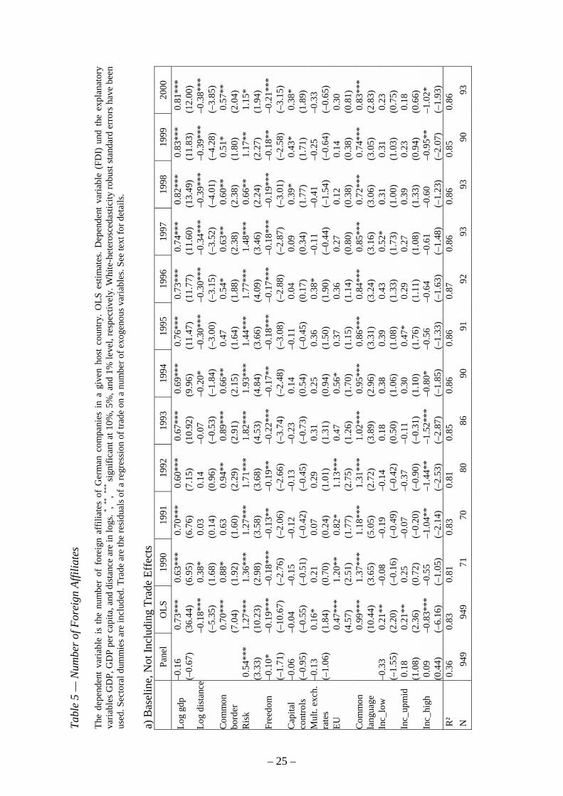
Tabl

e 5

— N

umbe

r of F

orei

gn A

ffilia

tes

The

depe

nden

t va

riabl

e is

the

num

ber

of f

orei

gn a

ffilia

tes

of G

erm

an c

ompa

nies

in

a gi

ven

host

cou

ntry

. OLS

est

imat

es. D

epen

dent

var

iabl

e (F

DI)

und

the

exp

lana

tory

varia

bles

GD

P, G

DP

per c

apita

, and

dis

tanc

e ar

e in

logs

. * , **, **

* sign

ifica

nt a

t 10%

, 5%

, and

1%

leve

l, re

spec

tivel

y. W

hite

-het

eros

ceda

stic

ity ro

bust

stan

dard

err

ors h

ave

been

used

. Sec

tora

l dum

mie

s are

incl

uded

. Tra

de a

re th

e re

sidu

als o

f a re

gres

sion

of t

rade

on

a nu

mbe

r of e

xoge

nous

var

iabl

es. S

ee te

xt fo

r det

ails

.

a) B

asel

ine,

Not

Incl

udin

g Tr

ade

Effe

cts

Pane

lO

LS19

9019

9119

9219

9319

9419

9519

9619

9719

9819

9920

00

Log

gdp

–0.1

6(–

0.67

)0.

73**

*(3

6.44

)0.

63**

*(6

.95)

0.70

***

(6.7

6)0.

60**

*(7

.15)

0.67

***

(10.

92)

0.69

***

(9.9

6)0.

76**

*(1

1.47

)0.

73**

*(1

1.77

)0.

74**

*(1

1.60

)0.

82**

*(1

3.49

)0.

83**

*(1

1.83

)0.

81**

*(1

2.00

)Lo

g di

stan

ce–0

.18*

**(–

5.35

)0.

38*

(1.6

8)0.

03(0

.14)

0.14

(0.9

6)–0

.07

(–0.

53)

–0.2

0*(–

1.84

)–0

.30*

**(–

3.00

)–0

.30*

**(–

3.15

)–0

.34*

**(–

3.52

)–0

.39*

**(–

4.01

)–0

.39*

**(–

4.28

)–0

.38*

**(–

3.85

)C

omm

onbo

rder

0.70

***

(7.0

4)0.

88*

(1.9

2)0.

63(1

.60)

0.94

**(2

.29)

0.89

***

(2.9

1)0.

66**

(2.1

5)0.

47(1

.64)

0.54

*(1

.88)

0.63

**(2

.38)

0.60

**(2

.38)

0.51

*(1

.80)

0.57

**(2

.04)

Ris

k0.

54**

*(3

.33)

1.27

***

(10.

23)

1.36

***

(2.9

8)1.

27**

*(3

.58)

1.71

***

(3.6

8)1.

82**

*(4

.53)

1.93

***

(4.8

4)1.

44**

*(3

.66)

1.77

***

(4.0

9)1.

48**

*(3

.46)

0.66

**(2

.24)

1.17

**(2

.27)

1.15

*(1

.94)

Free

dom

–0.1

0*(–

1.71

)–0

.19*

**(–

10.6

7)–0

.18*

**(–

2.76

)–0

.13*

*(–

2.06

)–0

.19*

*(–

2.66

)–0

.22*

**(–

3.74

)–0

.17*

*(–

2.48

)–0

.18*

**(–

3.08

)–0

.17*

**(–

2.88

)–0

.18*

**(–

2.87

)–0

.19*

**(–

3.01

)–0

.18*

*(–

2.58

)–0

.21*

**(–

3.15

)C

apita

lco

ntro

ls–0

.06

(–0.

95)

–0.0

4(–

0.55

)–0

.15

(–0.

51)

–0.1

2(–

0.42

)–0

.13

(–0.

45)

–0.2

3(–

0.73

)0.

14(0

.54)

–0.1

1(–

0.45

)0.

04(0

.17)

0.09

(0.3

4)0.

39*

(1.7

7)0.

43*

(1.7

1)0.

38*

(1.8

9)M

ult.

exch

.ra

tes

–0.1

3(–

1.06

)0.

16*

(1.8

4)0.

21(0

.70)

0.07

(0.2

4)0.

29(1

.01)

0.31

(1.3

1)0.

25(0

.94)

0.36

(1.5

0)0.

38*

(1.9

0)–0

.11

(–0.

44)

–0.4

1(–

1.54

)–0

.25

(–0.

64)

–0.3

3(–

0.65

)EU

0.47

***

(4.5

7)1.

20**

(2.5

1)0.

82*

(1.7

7)1.

13**

*(2

.75)

0.47

(1.2

6)0.

56*

(1.7

0)0.

37(1

.15)

0.36

(1.1

4)0.

27(0

.80)

0.12

(0.3

8)0.

14(0

.38)

0.30

(0.8

1)C

omm

onla

ngua

ge0.

99**

*(1

0.44

)1.

37**

*(3

.65)

1.18

***

(5.0

5)1.

31**

*(2

.72)

1.02

***

(3.8

9)0.

95**

*(2

.96)

0.86

***

(3.3

1)0.

84**

*(3

.24)

0.85

***

(3.1

6)0.

72**

*(3

.06)

0.74

***

(3.0

5)0.

83**

*(2

.83)

Inc_

low

–0.3

3(–

1.55

)0.

21**

(2.2

0)–0

.08

(–0.

16)

–0.1

9(–

0.49

)–0

.14

(–0.

42)

0.18

(0.5

0)0.

38(1

.06)

0.39

(1.0

8)0.

43(1

.33)

0.52

*(1

.73)

0.31

(1.0

0)0.

31(1

.03)

0.23

(0.7

5)In

c_up

mid

0.18

(1.0

8)0.

21**

(2.3

6)0.

25(0

.72)

–0.0

7(–

0.20

)–0

.37

(–0.

90)

–0.1

1(–

0.31

)0.

30(1

.10)

0.47

*(1

.76)

0.29

(1.1

1)0.

27(1

.08)

0.39

(1.3

3)0.

23(0

.94)

0.18

(0.6

6)In

c_hi

gh0.

09(0

.44)

–0.8

3***

(–6.

16)

–0.5

5(–

1.05

)–1

.04*

*(–

2.14

)–1

.44*

*(–

2.53

)–1

.52*

**(–

2.87

)–0

.80*

(–1.

85)

–0.5

6(–

1.33

)–0

.64

(–1.

63)

–0.6

1(–

1.48

)–0

.60

(–1.

23)

–0.9

5**

(–2.

07)

–1.0

2*(–

1.93

)R

²0.

360.

830.

810.

830.

810.

850.

860.

860.

870.

860.

860.

850.

86N

949

949

7170

8086

9091

9293

9390

93

– 25 –

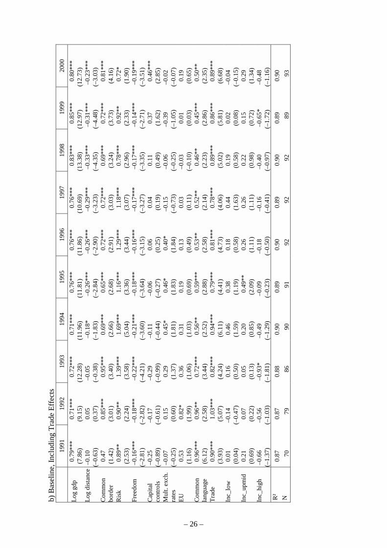
b) B

asel

ine,

Incl

udin

g Tr

ade

Effe

cts

1991

1992

1993

1994

1995

1996

1997

1998

1999

2000

Log

gdp

0.79

***

(7.8

6)0.

71**

*(9

.15)

0.72

***

(12.

28)

0.71

***

(11.

96)

0.76

***

(11.

81)

0.76

***

(11.

86)

0.76

***

(10.

69)

0.83

***

(13.

38)

0.85

***

(12.

97)

0.80

***

(12.

73)

Log

dist

ance

–0.1

0(–

0.63

)0.

05(0

.37)

–0.0

5(–

0.38

)–0

.18*

(–1.

83)

–0.2

6***

(–2.

84)

–0.2

6***

(–2.

90)

–0.2

9***

(–3.

23)

–0.3

3***

(–4.

35)

–0.3

1***

(–4.

48)

–0.2

3***

(–3.

03)

Com

mon

bord

er0.

47(1

.42)

0.85

***

(3.0

1)0.

95**

*(3

.40)

0.69

***

(2.6

6)0.

65**

*(2

.68)

0.72

***

(2.9

1)0.

72**

*(3

.03)

0.69

***

(3.2

4)0.

72**

*(3

.73)

0.81

***

(4.1

6)R

isk

0.89

**(2

.53)

0.90

**(2

.24)

1.39

***

(3.5

8)1.

69**

*(5

.04)

1.16

***

(3.3

6)1.

29**

*(3

.44)

1.18

***

(3.0

7)0.

78**

*(2

.96)

0.92

**(2

.33)

0.72

*(1

.90)

Free

dom

–0.1

6***

(–2.

81)

–0.1

8***

(–2.

82)

–0.2

2***

(–4.

21)

–0.2

1***

(–3.

60)

–0.1

8***

(–3.

64)

–0.1

6***

(–3.

15)

–0.1

7***

(–3.

27)

–0.1

7***

(–3.

35)

–0.1

4***

(–2.

71)

–0.1

9***

(–3.

51)

Cap

ital

cont

rols

–0.2

5(–

0.89

)–0

.17

(–0.

61)

–0.2

9(–

0.99

)–0

.11

(–0.

44)

–0.0

6(–

0.27

)0.

06(0

.25)

0.04

(0.1

9)0.

11(0

.49)

0.37

(1.6

2)0.

46**

*(2

.85)

Mul

t. ex

ch.

rate

s–0

.07

(–0.

25)

0.15

(0.6

0)0.

29(1

.37)

0.45

*(1

.81)

0.46

*(1

.83)

0.40

*(1

.84)

–0.1

5(–

0.73

)–0

.06

(–0.

25)

–0.3

9(–

1.05

)–0

.02

(–0.

07)

EU0.

53(1

.16)

0.82

*(1

.99)

0.36

(1.0

6)0.

31(1

.03)

0.19

(0.6

9)0.

13(0

.49)

0.03

(0.1

1)–0

.03

(–0.

10)

0.01

(0.0

3)0.

19(0

.65)

Com

mon

lang

uage

0.96

***

(6.1

2)0.

96**

(2.5

8)0.

72**

*(3

.44)

0.56

**(2

.52)

0.59

***

(2.8

8)0.

53**

(2.5

8)0.

52**

(2.1

4)0.

46**

(2.2

3)0.

45**

*(2

.86)

0.50

**(2

.35)

Trad

e0.

90**

*(3

.93)

1.03

***

(5.0

7)0.

82**

*(4

.24)

0.94

***

(6.1

1)0.

79**

*(4

.41)

0.81

***

(4.7

3)0.

78**

*(4

.06)

0.89

***

(5.0

2)0.

86**

*(5

.81)

0.89

***

(6.6

8)In

c_lo

w0.

01(0

.04)

–0.1

4(–

0.47

)0.

16(0

.50)

0.46

(1.5

9)0.

38(1

.19)

0.18

(0.5

8)0.

44(1

.63)

0.19

(0.5

8)0.

02(0

.08)

–0.0

4(–

0.15

)In

c_up

mid

0.21

(0.6

9)0.

07(0

.22)

0.05

(0.1

3)0.

20(0

.85)

0.49

**(2

.09)

0.26

(1.1

1)0.

26(1

.11)

0.22

(0.9

8)0.

15(0

.72)

0.29

(1.3

4)In

c_hi

gh–0

.66

(–1.

37)

–0.5

6(–

1.03

)–0

.93*

(–1.

81)

–0.4

9(–

1.29

)–0

.09

(–0.

23)

–0.1

8(–

0.50

)–0

.16

(–0.

41)

–0.4

0(–

0.97

)–0

.65*

(–1.

72)

–0.4

8(–

1.16

)R

²0.

870.

870.

880.

900.

890.

900.

890.

900.

890.

90N

7079

8690

9192

9292

8993

– 26 –

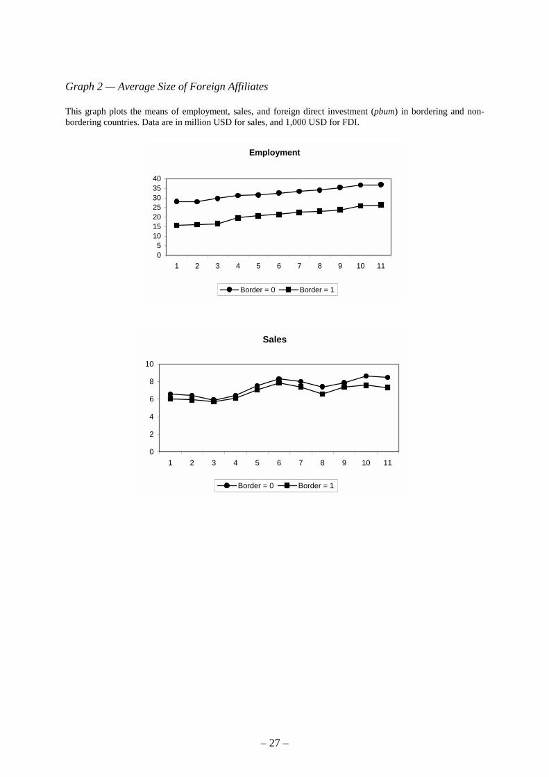
Graph 2 — Average Size of Foreign Affiliates

This graph plots the means of employment, sales, and foreign direct investment (pbum) in bordering and non-bordering countries. Data are in million USD for sales, and 1,000 USD for FDI.

Employment

05

10152025303540

1 2 3 4 5 6 7 8 9 10 11

Border = 0 Border = 1

Sales

0

2

4

6

8

10

1 2 3 4 5 6 7 8 9 10 11

Border = 0 Border = 1

– 27 –

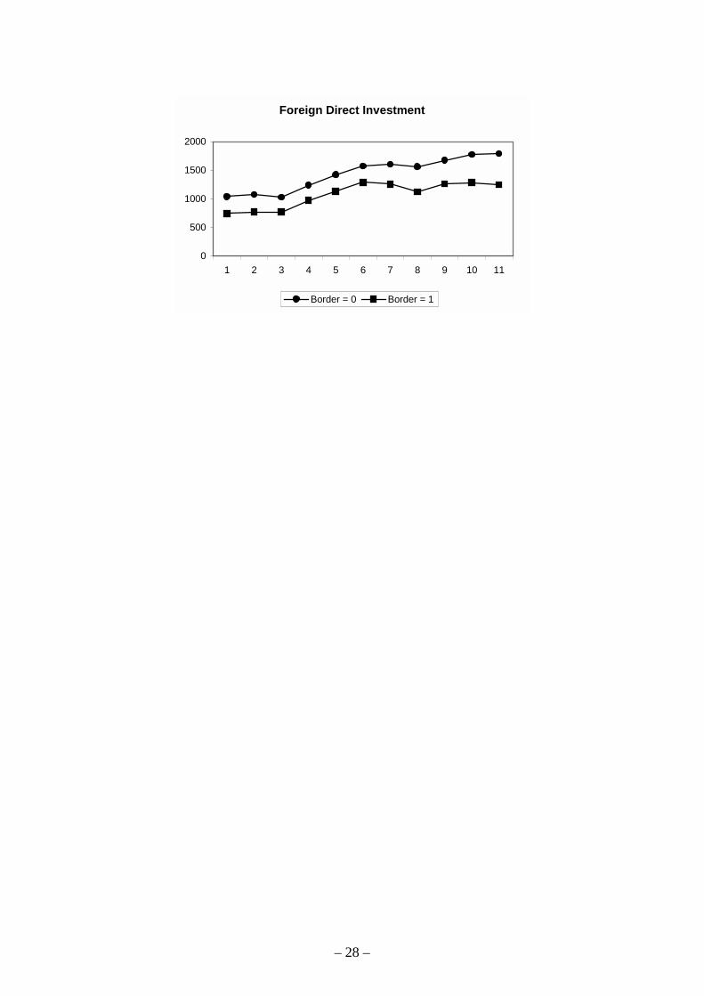
Foreign Direct Investment

0

500

1000

1500

2000

1 2 3 4 5 6 7 8 9 10 11

Border = 0 Border = 1

– 28 –

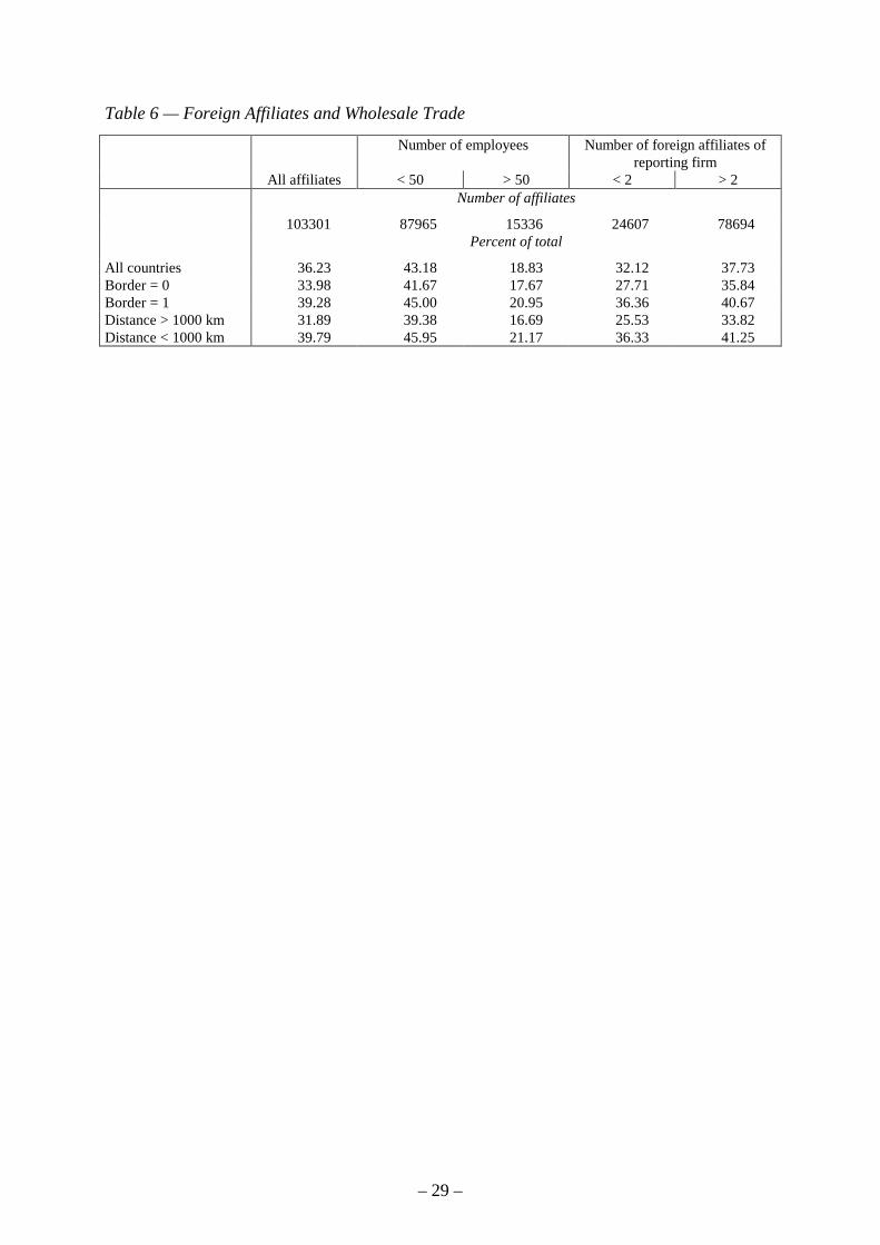
Table 6 — Foreign Affiliates and Wholesale Trade

Number of employees Number of foreign affiliates ofreporting firm

All affiliates < 50 > 50 < 2 > 2Number of affiliates

103301 87965 15336 24607 78694Percent of total

All countries 36.23 43.18 18.83 32.12 37.73Border = 0 33.98 41.67 17.67 27.71 35.84Border = 1 39.28 45.00 20.95 36.36 40.67Distance > 1000 km 31.89 39.38 16.69 25.53 33.82Distance < 1000 km 39.79 45.95 21.17 36.33 41.25

– 29 –

– 30 –

The following papers have been published since 2002:

January 2002 Rent indices for housing in West Johannes HoffmannGermany 1985 to 1998 Claudia Kurz

January 2002 Short-Term Capital, Economic Transform- Claudia M. Buchation, and EU Accession Lusine Lusinyan

January 2002 Fiscal Foundation of Convergenceto European Union inLászló HalpernPre-Accession Transition Countries Judit Neményi

January 2002 Testing for Competition AmongGerman Banks Hannah S. Hempell

January 2002 The stable long-run CAPM andthe cross-section of expected returns Jeong-Ryeol Kim

February 2002 Pitfalls in the European EnlargementProcess – Financial Instability andReal Divergence Helmut Wagner

February 2002 The Empirical Performance of Option Ben R. CraigBased Densities of Foreign Exchange Joachim G. Keller

February 2002 Evaluating Density Forecasts with an Gabriela de RaaijApplication to Stock Market Returns Burkhard Raunig

February 2002 Estimating Bilateral Exposures in theGerman Interbank Market: Is there a Christian UpperDanger of Contagion? Andreas Worms

February 2002 The long-term sustainability of publicfinance in Germany – an analysis basedon generational accounting Bernhard Manzke

– 31 –

March 2002 The pass-through from market interestrates to bank lending rates in Germany Mark A. Weth

April 2002 Dependencies between Europeanstock markets when price changesare unusually large Sebastian T. Schich

May 2002 Analysing Divisia Aggregatesfor the Euro Area Hans-Eggert Reimers

May 2002 Price rigidity, the mark-up and thedynamics of the current account Giovanni Lombardo

June 2002 An Examination of the RelationshipBetween Firm Size, Growth, andLiquidity in the Neuer Markt Julie Ann Elston

June 2002 Monetary Transmission in theNew Economy: Accelerated Depreci-ation, Transmission Channels and Ulf von Kalckreuththe Speed of Adjustment Jürgen Schröder

June 2002 Central Bank Intervention andExchange Rate Expectations –Evidence from the DailyDM/US-Dollar Exchange Rate Stefan Reitz

June 2002 Monetary indicators and policy rulesin the P-star model Karl-Heinz Tödter

July 2002 Real currency appreciation in acces-sion countries: Balassa-Samuelson andinvestment demand Christoph Fischer

August 2002 The Eurosystem’s Standing Facilitiesin a General Equilibrium Model of theEuropean Interbank Market Jens Tapking

– 32 –

August 2002 Imperfect Competition, Monetary Policyand Welfare in a Currency Area Giovanni Lombardo

August 2002 Monetary and fiscal policy rules in amodel with capital accumulation andpotentially non-superneutral money Leopold von Thadden

September 2002 Dynamic Q-investment functions forGermany using panel balance sheet dataand a new algorithm for the capital stock Andreas Behrat replacement values Egon Bellgardt

October 2002 Tail Wags Dog? Time-Varying Informa- Christian Uppertion Shares in the Bund Market Thomas Werner

October 2002 Time Variation in the Tail Behaviour of Thomas WernerBund Futures Returns Christian Upper

November 2002 Bootstrapping Autoregressions withConditional Heteroskedasticity of Sílvia GonçalvesUnknown Form Lutz Kilian

November 2002 Cost-Push Shocks and Monetary Policyin Open Economies Alan Sutherland

November 2002 Further Evidence On The RelationshipBetween Firm Investment And Robert S. ChirinkoFinancial Status Ulf von Kalckreuth

November 2002 Genetic Learning as an Explanation ofStylized Facts of Foreign Exchange Thomas LuxMarkets Sascha Schornstein

December 2002 Wechselkurszielzonen, wirtschaftlicherAufholprozess und endogene Realign-mentrisiken * Karin Radeck

* Available in German only.

– 33 –

– 34 –

December 2002 Optimal factor taxation under wage Erkki Koskelabargaining – a dynamic perspective Leopold von Thadden

January 2003 Testing mean-variance efficiency in CAPM Marie-Claude Beaulwith possibly non-gaussian errors: an Jean-Marie Dufourexact simulation-based approach Lynda Khalaf

January 2003 Finite-sample distributions ofself-normalized sums Jeong-Ryeol Kim

January 2003 The stock return-inflation puzzle andthe asymmetric causality in stock returns,inflation and real activity Jeong-Ryeol Kim

February 2003 Multiple equilibrium overnight ratesin a dynamic interbank market game Jens Tapking

February 2003 A comparison of dynamic panel dataestimators: Monte Carlo evidence andan application to the investment function Andreas Behr

March 2003 A Vectorautoregressive InvestmentModel (VIM) And Monetary Policy Joerg BreitungTransmission: Panel Evidence From Robert S. ChirinkoGerman Firms Ulf von Kalckreuth

March 2003 The international integration of moneymarkets in the central and east Europeanaccession countries: deviations from coveredinterest parity, capital controls and inefficien- Sabine HerrmannCies in the financial sector Axel Jochem

March 2003 The international integration offoreign exchange markets in the centraland east European accession countries:speculative efficiency, transaction costs Sabine Herrmannand exchange rate premiums Axel Jochem

March 2003 Determinants of German FDI: Claudia BuchNew Evidence from Jörn KleinertMicro-Data Farid Toubal

– 35 –

– 36 –

Visiting researcher at the Deutsche Bundesbank

The Deutsche Bundesbank in Frankfurt is looking for a visiting researcher. Visitors shouldprepare a research project during their stay at the Bundesbank. Candidates must hold aPh D and be engaged in the field of either macroeconomics and monetary economics,financial markets or international economics. Proposed research projects should be fromthese fields. The visiting term will be from 3 to 6 months. Salary is commensurate withexperience.

Applicants are requested to send a CV, copies of recent papers, letters of reference and aproposal for a research project to:

Deutsche BundesbankPersonalabteilungWilhelm-Epstein-Str. 14

D - 60431 FrankfurtGERMANY

– 37 –