determinants of banks profitability - erasmus university ... s. van (302984... · web viewii 11...

BANKS’ PROFITABILITYAN EXAMINATION OF THE DETERMINANTS OF

BANKS’ PROFITABILITY IN THE EUROPEAN BANKING SECTOR

S. (Stefan) van Ommerenϕ

October 14th, 2011

ABSTRACTThis thesis examines determinants of banks’ profitability in the European banking sector. The descriptive analysis indicates that the banking sector is unique compared to other industry sectors since the sector is heavily regulated and since that commercial, mutual, co-operative and government-owned banks jointly operate in the sector. Hence, the empirical part of this thesis takes into account, in particular, regulation and ownership issues. The analysis extends research of Dietrich and Wanzenried (2011) by examining additional determinants of banks’ profitability and by focusing on the European banking sector. Apart from examining the determinants of banks’ profitability, potential impacts of the financial crisis are considered. Using an unbalanced panel of 354 banks between 2000 and 2009, this thesis shows that profit persistence still exists in the banking sector. Besides, findings suggest that the equity-to-asset ratio is positively related to banks’ profitability supporting the bankruptcy cost hypothesis or signaling hypothesis. There is no evidence found that the funding- and liquidity structure are determinants for profitability, both proxies appears to be insignificant. Besides, little evidence is found for the agency theory.

JEL Classifications: C23 G15 G21Keywords: Banking, profitability, panel data, generalized method of moments, ownership, regulation

ERASMUS UNIVERSITY ROTTERDAMErasmus School of EconomicsDepartment of FinanceSUPERVISORProf. Dr. W.F.C. Verschoor

RABOBANK NEDERLANDGroup Risk Management

Balance Sheet RiskSUPERVISOR

Ir. K. Kruidhof

ϕ Master student at Erasmus University Rotterdam, Erasmus School of Economics, Department of Accounting & Finance and intern at Rabobank Nederland, Group Risk Management, Balance Sheet Risk. Please use the following e-mail address for corresponding: [email protected]

mailto:[email protected]

NON-PLAGIARISM STATEMENTBy submitting this thesis the author declares to have written this thesis completely by himself/herself, and not to have used sources or resources other than the ones mentioned. All sources used, quotes and citations that were literally taken from publications, or that were in close accordance with the meaning of those publications, are indicated as such.

COPYRIGHT STATEMENTThe author has copyright of this thesis, but also acknowledges the intellectual copyright of contributions made by the thesis supervisor, which may include important research ideas and data. Author and thesis supervisor will have made clear agreements about issues such as confidentiality.Electronic versions of the thesis are in principle available for inclusion in any EUR thesis database and repository, such as the Master Thesis Repository of the Erasmus University Rotterdam

ii

PREFACE

This preface marks the start of this thesis but simultaneously marks the end of five years of study. Writing a master thesis for obtaining a master degree in Accounting and Finance, is not only a completion of several years of study, it is certainly a process. The beginning of this process is sometimes tough but once initiated the process of writing a master thesis is very interesting; it is an opportunity to explore and to specialize in an economic topic. In the past months, I have also gained practical knowledge about the economic topics in banking, risk management and banks’ balance sheet structures due to an internship at the ‘Group Risk Management’ department of Rabobank Nederland.

Writing a dissertation is an individual assignment, nonetheless support from others contributed to the completion of this thesis. Therefore, I would like to use this preface to acknowledge several people who helped me in the past months and throughout my study. First, I would like to thank Prof. Dr. Verschoor from the Erasmus School of Economics for his subject-matter support and constructive comments. Prof. Dr. Verschoor safeguarded the academic value of this thesis and gave me valuable insights during the whole process. Furthermore, I gratefully acknowledge Klaroen Kruidhof, manager Balance Sheet Risk at Rabobank Nederland, for his support and comments during the internship and for the opportunity to look behind the scenes of a large financial institution. Moreover, I would also like to mention the colleagues of Group Risk Management, which create a motivating and interesting environment to work in the past months.

Special thank goes out to my family and friends who supported me during the study and the master thesis. In particular, I would like to thank my parents for their support and my partner, Denise – being unfamiliar to the subject; she always read the concepts and was always there for me. I would like to dedicate this thesis to my deceased brother, Mark – to whom I once promised to achieve a university degree - being near to that moment, I know you would be very proud.

Finally, I hope that you will share my enthusiasm and interest in the topic and in the banking sector when reading this thesis. Moreover, I hope that this final version fulfills in its goal to give practical knowledge about the determinants of banks’ profitability.

Utrecht, October 2011.

Stefan van Ommeren

iii

TABLE OF CONTENTSTable on contents

PREFACE...........................................................................................................................ii

LIST OF FIGURES AND TABLES...........................................................................................v

ABBREVIATIONS..............................................................................................................vi

1. INTRODUCTION............................................................................................................1

1.1 Relevance 2

1.2 Research question 3

1.3 Results and findings 3

1.4 Outline 4

2. THEORETICAL BACKGROUND........................................................................................5

2.1 Function of banks 5

2.2 Rational for regulation and supervision 6

2.3 European banking sector 8

2.4 General influences on banks’ profitability 9

2.5 Summary 11

3. LITERATURE REVIEW...................................................................................................12

3.1 Literature on regulation and profitability 12

3.2 Literature on ownership structure and profitability 13

3.3 Literature on balance sheet structure and profitabilitY 15

3.4 Macroeconomic, industry-specific and bank-specific factors and profitability 15

3.5 Summary 18

4. HYPOTHESIS AND DETERMINANTS SELECTION............................................................19

4.1 Dependent variable 19

4.2 Independent variables 21

4.3 Summary 26

5. RESEARCH DESIGN AND DATA....................................................................................27

5.1 Methodology 27

5.2 Data 30

iv

5.3 Descriptive statistics 31

5.4 Summary 36

6. EMPIRICAL RESULTS....................................................................................................38

6.1 Empirical results of the determinants of banks’ profitability 38

6.2 Robustness checks 44

6.3 Summary 47

7. SUMMARY AND CONCLUSIONS..................................................................................49

7.1 Limitations 50

7.2 Recommendations for future research 51

REFERENCES...................................................................................................................53

APPENDICES...................................................................................................................57

I. Rabobank Group 57

II. Basel regulation 58

III. Literature review 61

IV. Calculation methods for the descriptive statistics 67

V. Dynamic panel data estimation 68

v

LIST OF FIGURES AND TABLES

Table 1 Differences between minimum capital requirements 7

Table 2 Selection of the determinants of profitability and used data source. 25

Table 3 Sample composition and number of bank observations 31

Table 4 Descriptive statistics for total sample and sub periods (excluding outliers) 33

Table 5 Correlation matrix of dependent and independent variables 35

Table 6 Regression results with dependent variable ROAA 41

Table 7 Robustness checks 46

Figure 1 Organizational structure Rabobank Group 57

Figure 2 Three pillar structure (Basel II and II) 59

Table 8 Summary of literature review of regulation and banks’ profitability 61

Table 9 Summary of literature review of ownership structure and banks’ profitability 63

Table 10 Summary of literature review of determinants and banks’ profitability 65

Figure 3 Scatter plot return on average assets and equity-to-asset ratio 67

vi

ABBREVIATIONS

BIS Bank for International SettlementsDEPV Dependent variableEVA Economic value addedEURIBOR Euro Interbank Offered Rate EXPL Explanatory variablesGMM Generalized Method of MomentsGDP Gross domestic productIFRS International Financial Reporting StandardsLCR Liquidity coverage ratioNIM Net interest marginNSFR Net stable funding ratioOBS Off balance sheetOLS Ordinary least squaresRAROC Return-adjusted return on capitalROE Return on equityROA Return on assetsROAA Return on average assetsROAE Return on average equitySCP Structure-conduct-performanceSt. dev Standard deviationNPV Net present valueU.S.A. United States of America

1

1. INTRODUCTION

In recent years, changing market factors and an altering policy climate had a substantial impact on world’s banking sector. After decades of deregulation, globalization and financial innovation the banking sector flourished until the near collapse of the financial market a few years ago. As a consequence a fundamental reassessment of the banking sector is requested (Rosenthal, 2011). Current efforts to reform regulation and supervision will lead to a new era of reregulation and will likely impact banks’ profitability. In this context, Allen, Chan, Milne and Thomas (2010, p. 1) argue that:

“Basel III will force banks to shift their business model from liability management, in which business decisions are made about asset volumes, with the financing found in short term wholesale markets as necessary, to asset management, in which asset volumes are constrained by the availability of funding”

The purpose of this thesis is to define the determinants of banks’ profitability by examining, in particular, regulation, ownership structure and the balance sheet structure. Understanding of determinants of banks’ profitability could be very valuable for banks’ managers in daily business decisions. Hereby banks’ managers could assess and reduce the impact of new regulation on profitability since future regulation will likely affect determinants of profitability. In addition, academic research could use the findings of this thesis to test whether the introduction of new regulation alters determinants of banks’ profitability.

As said, this thesis examines the influence of regulation, the ownership structure, the balance sheet structure on performance. Regulation is examined in detail, because current efforts to reform regulation and a changing policy climate could substantially influence the banking sector. In addition, prior research extensively analyzed the influence of the ownership structure outside the banking sector. Results for the banking sector could be different because regulators set requirements on the extent of capitalization. Finally, the balance sheet structure is very important in today’s management, both for internal and external purposes. Namely, the balance sheet structure legitimates daily business decisions and serves as proxy for sound and prudent risk management. Besides, regulation often focuses on the balance sheet structure through which it could affect banks’ profitability. In this context, determinants of profitability mainly relate to the balance sheet structure due to the special nature of banks.

Furthermore, this thesis will also refer to findings from a study during an internship by Rabobank Nederland (see also appendix I). In this internship, balance sheet structures of European banks are examined using descriptive and qualitative research techniques. Developments over time with respect to the financial crisis and to the introduction of new regulation are contrasted and compared. Several findings are presented in the theoretical background in subsequent chapters.

2 Introduction

1.1 RELEVANCE

Prior empirical research generally investigates determinants of banks’ profitability on different levels and directions. The main direction of interest of this thesis is, to develop a comprehensive model that incorporates macroeconomic, industry-specific and bank-specific determinants (of which the bank-specific determinants mainly relate to the balance sheet structure). Nevertheless, research also focuses on specific determinants, such as the relationship between regulation and profitability or the relationship between the ownership structure and profitability.

According to Barth, Caprio Jr. and Levine (2004) capital requirements and restrictions on banking activities do not have a significant impact on bank’s profitability, measured by the net interest margin. Among others, Laeven & Levine (2009) find that risk taking by banks is influenced by regulation. Moreover, it appears that the impact of regulation on risk taking is determined to some extent by the ownership structure. Empirical research towards the relationship between ownership structure and profitability, give mixed results (Saunders, Strock and Travlos, 1990; Altunbas, Evans and Molyneux, 2001; Iannotta, Nocera and Sironi, 2007 and Micco, Panizza and Yaňez, 2007). Some studies find a positive relationship between private ownership and profitability while others find a negative or insignificant relationship. Nevertheless, there is a strong-bodied theoretical explanation for the relationship between ownership structure and banks’ profitability, given by the agency theory of Jensen and Meckling (1976). Finally, prior research also focuses on bank-specific determinants of performance using e.g. balance sheet ratios (Berger, 1995 and Demirgüç-Kunt and Huizinga, 1999).

This thesis builds on research of Pasiouras and Kosmidou (2007) and Dietrich and Wanzenried (2011), who investigates macroeconomic, industry-specific and bank-specific determinants of profitability utilizing a regression model. Using data from the European banking sector between 1995 and 2001, Pasiouras and Kosmidou (2007) find evidence for influences within all three categories. More recently, Dietrich and Wanzenried (2011) also examine the impact of the financial crisis on determinants of banks’ profitability for the Swiss banking sector between 1999 and 2009. They find that significances and coefficients altered during the financial crisis. For instance, the coefficient of the capital ratio is insignificant in the pre-crisis sample and negatively during the crisis. Furthermore, the coefficient of ownership structure is insignificant before the crisis whilst, during the crisis, the coefficient is significant and positive, implying that state-owned banks performed better.

This thesis extends existing literature in three ways. First, the European banking sector is considered, utilizing data between 2000 and 2009. No previous study has considered a comprehensive framework of macroeconomic, industry-specific and bank-specific determinants of banks’ profitability for the European banking sector over the last decade, whilst globalization, increasing competition, international convergence of banking regulation and accounting standards improve the comparability of the European banking sector. Until now, most research uses data from the 20 th

century (Pasiouras and Kosmidou, 2007 and Athanasoglou, Sophocles and Delis, 2008). Moreover, existing academic research is mostly concentrated to individual countries (Saunders et al., 1990 and Berger, 1995). Up to now, only a few studies used more recent data, but these studies examined separate determinants e.g. the ownership structure (Iannotta et al., 2007 and Barry, Lepetit and Tarazi, 2011). Second, this study attempts to extend determinants of banks’ profitability used by Molyneux and Thornton (1992) and Pasiouras and Kosmidou, 2007) by examining funding and

3 Introduction

liquidity ratios. Hereby this study anticipates to the introduction of new regulation and possible impacts of funding and liquidity issues on banks’ profitability. Third, this thesis attempts to generalize results of Dietrich and Wanzenried (2011) regarding the impact of the financial crisis on determinants of banks’ profitability, to the European banking sector.

1.2 RESEARCH QUESTION

Resuming, the aim of this study is to provide information on determinants that influence profitability. As mentioned above there is a gap in existing literature towards the determinants of banks’ profitability. Despite the fact that there is abundant literature on banking profitability in several individual countries there are only a few studies available using recent data for the European banking sector. In order to extend current literature and to satisfy the purpose of this thesis the following research question is defined.

Main questionWhat are the determinants of banks’ profitability and how do regulation, ownership structure and the balance sheet structure influence the profitability?

Moreover, this thesis uses data over the last decade and implicitly incorporates data of the financial crisis (2007-current). As a consequence, relationships between determinants and banks’ profitability could have altered during this period. Those impacts could also be very interesting and valuable in assessing relationships therefore the following sub question is defined:

Sub question Did relationships between determinants of banks’ profitability change during the financial crisis?

1.3 RESULTS AND FINDINGS

The empirical research is based on different theoretical explanations and models. For the relationship between regulation and profitability, this study examines whether future funding and liquidity requirements influence profitability. Moreover, to investigate the relationship between ownership structure and banks’ profitability the agency theory of Jensen and Meckling (1976) is tested. Their hypothesis suggests that profitability is influenced by the ownership structure; it assumes that shareholder owned banks are more profitable than mutual, co-operative and state-owned banks. Finally, different theoretical explanations are used to test the relationship between several balance sheet ratios and banks’ profitability. For instance, for the relationship between the equity-to-asset ratio and profitability the signaling and bankruptcy cost hypothesis are contrasted against the risk-return hypothesis.

The research question is investigated using a regression model based on the two-step system generalized method of moments (GMM) estimator. Using an unbalanced panel of 354 European banks between 2000 and 2009 this thesis find little support that the variable customer deposits to total funding and the variable liquid assets to short term funding (excluding derivatives) are determinants for banks’ profitability. Both the liquidity and funding ratios are insignificant in all

4 Introduction

periods suggesting that future funding and liquidity requirements do not influence profitability, ceteris paribus. However, discussions between practitioners and supervisors indicate that requirements could influence future banking activities through different other mechanisms. Besides, there is only some moderate evidence for the agency theory; the parameter for the dummy variable of government-owned banks is significant and negative but only in the total sample and on a 10% level. The coefficient for stakeholder-owned banks, however, is insignificant; indicating that there is no evidence that stakeholder-owned banks perform worse than their shareholder-owned counterparts. The most explaining power for banks’ profitability, in the total sample, is attributed to the one-year lag of profitability justifying the dynamic nature of the model. Note, however, that profit persistence is not observed in both subsamples. Continuing to the bank-specific variables the equity-to-asset ratio positively explains banks’ profitability; supporting the signaling or bankruptcy cost hypothesis. Other interesting findings include (i) a positive and significant coefficient for non-interest income and (ii) an insignificant coefficient for funding costs. The first coefficient indicates that a bank generate a higher spread on non-interest activities or that income diversification is positive contributor to the profits. The second insignificant parameter indicates that banks are able to charge their funding costs on to customers. Within the industry-speicifc variables the concentration and size variables are both insignificant not supporting the large consolidation and expansion in the banking sector over the last decade. Furthermore, from the macroeconomic variables only the business cycle is a determinant for banks’ profitability.

1.4 OUTLINE The remainder of this thesis is structured as follows. The next chapter introduces underlying concepts of banking and provides a brief overview of the regulation to which banks are subject. Subsequently, in chapter three the empirical research on banks’ profitability is reviewed by presenting findings of research on regulation, ownership structure and other (mostly bank-specific) determinants of profitability. Chapter four selects the variables and determinants for banks’ profitability. This chapter also presents hypotheses for the expected sign for the relationships between the explanatory variables and the dependent variable. Subsequently, chapter five will describe the sample and the regression model. Consequently, chapter six presents the results of the regression analysis described in chapter five. In addition, chapter six also report robustness checks to validate results. Finally, chapter seven concludes by summarizing the findings of this thesis and by answering the research question. Moreover, chapter seven also discusses the implications for further research and gives remarks and limitations of the findings.

5

2. THEORETICAL BACKGROUND

Several factors influence banks’ operations and banks’ profitability, recognizing and understanding the underlying concepts and definitions of the banking sector is essential in order to vouch results and analyses. Hence, chapter two serves as background for this study by describing concepts of financial intermediation and factors that could influence banks’ profitability. Subsequent chapters will build on concepts and definitions described here. First, this chapter discusses the function of banks, followed by an outline of the rational for regulation and supervision. Subsequently recent developments in the European banking sector are reviewed. Finally, this chapter explains some theoretical frameworks that are helpful in assessing the relationship between macroeconomic, industry-specific, bank-specific factors and banks’ profitability.

2.1 FUNCTION OF BANKS

To start very basic, this paragraph discusses the function of banks in the economy and examines the question why banks exist. At first sight, the answer to this question is very intuitive and simple; banks act as an intermediary between those who are in need for money and those who have excess of money. Looking more closely to this question there could be a more detailed explanation. Namely, in a perfect capital market of Modigliani-Miller (MM), financial institutions are superfluous (Santos, 2001); namely, entities can borrow and save directly through the capital market. In reality, such perfect market does not exist; transaction costs and monitoring costs distort capital markets. Furthermore, capital markets suffer from the information asymmetry and the agency problem. The agency problem refers to the dissimilar incentives of borrowers and savers, in a broader context it refers to the dissimilar incentives of principles and agents (Jensen and Meckling, 1976). In a case of financial distress, borrowers are limited liable; implying that they have incentives to alter their behavior by taking on more risk than savers are willing to accept. Monitoring the borrowers’ behavior is time consuming, complex and expensive for individuals. In inefficient markets, financial intermediation is beneficial since banks have lower monitoring and transaction costs than individuals, due to economies of scale and scope.

Another important aspect of banking is the function of maturity transformation. Banks receive short-term savings from depositors and transform those savings into long-term loans to borrowers. By holding a part of the short-term savings in liquid assets and cash, banks could withstand daily withdrawals from depositors. Banks offer a unique service; lending long term while guaranteeing the liquidity of their liabilities to depositors, which can withdraw their money at any time without a decline in nominal value (Schooner and Talyor, 2010). Capital markets cannot achieve maturity transformation with the same benefits as banks can. Individual investors face liquidity, price and credit risk1, which they cannot diversify to the extent banks can. As savers do not withdraw their deposits at the same time, banks hold only a minor part of the savings in liquid cash. Thus, banks diversify liquidity risks over a large pool of savers. Individual savers can also diversify their investments in terms of credit and price risks but it remains unlikely that they could withdraw the investments at any time without facing liquidity issues.

6 Theoretical background

Nowadays, bank activities are more diverse than ever. In the past decades, competition has increased and new activities have emerged. The traditional form of banking, receiving deposits and extending credits, has become less important. Ever since the complexity of balance sheet has increased, as did balance sheet and risk management (van Greuning and Bratanovic, 2009). Besides the incorporations of liquidity, price and credit risks in banking activities, banks increasingly faces market risks (e.g. interest rate risk and currency risk). One may assume that banks’ risk managers properly diversify these risks and closely monitor borrowers’ behavior to avoid bank failure or financial distress. Nevertheless, as the next paragraph points out, monitoring bank behavior is required to safeguard the continuity and stability of the banking sector due to moral hazard issues.

2.2 RATIONAL FOR REGULATION AND SUPERVISION

Moral hazard refers to changes in behavior when entities are insured or limited liable to losses. In the context of the banking sector, it refers to a changing behavior in terms of risk taking since the downside losses for banks’ owners (e.g. shareholders and member) are limited to the amount of equity invested whilst the upside potential of risk taking is unrestricted. Given the fact that the downside losses are restricted by a put option value arising from the limited liability, banks could maximize shareholder value by taking on more risks than depositors are willing to accept. According to Rime (2001), excessive risk taking and possible shortfalls (bankruptcies) are partly born by depositors and the deposit insurance schemes. Moreover, the past years have shown that owners are often supported by government interventions to avoid a collapse of the banking sector. Monitoring banks would be necessary to avoid excessive risk taking and to prevent a bank failure or even a systematic failure of the banking sector (Saunders et al., 1990). A systematic failure of the banking sector is highly undesirable given the central role of financial institutions in current economy. Some researchers argue that the moral hazard problem is less important than regulators assume and state that the moral hazard problem does not fully explain the relationship between bank capital and risk taking. Following Milne and Whalley (2001) one should take into account possible future streams of income earnings and the fact that shareholders rarely extract maximum payouts from banks. These effects restrain the moral hazard problem. Despite this contrary explanation, supervisors, academic researchers and politicians address the moral hazard problem and finds supervision necessary. Note that regulation in the banking sector is not only introduced to reduce moral hazard issues but also, among other reasons, to offer services to customers, who are financially illiterate, that meet several minimum requirements.

Monitoring and supervision certainly reduce the moral hazard problem in the banking sector. However, some academics and practitioners argue that monitoring does not completely solve the moral hazard problem. Following Barth et al. (2004), neither private nor official entities can effectively monitor complex banks. Furthermore, Blum (2008) states that supervisors cannot validate banks’ risk assessments. According to Barth et al. (2004) and Blum (2008), information asymmetries mainly cause the above-mentioned inabilities. Information asymmetries will lead to undesirable outcomes given the fact that banks have incentives to understate their risk, as reporting higher risk will lead to higher minimal capital ratios (Blum, 2008). Assessing risk management principles is very difficult for supervisors; hence, regulation is adapted and focused towards the balance sheet structure of banks. In this context, the balance sheet serves as proxy for supervisors to test sound


and adequate risk management principles. The next paragraph discusses regulation and guidelines for banks. Its purpose is to describe which constrains regulators places on bank’s activities and balance sheet structures in order to understand how regulation could affect determinants of banks’ profitability.

2.2.1 RECENT DEVELOPMENTS IN INTERNATIONAL BANK REGULATION

In 1988, the Basel Committee on Banking Supervision introduced the first broadly accepted international accord on banking supervision; the Basle Capital Accord - also known as Basel I. Originally, the accord focused on credit risk as it is the most important risk driver for banks (Santos, 2001). Later on, the Basel Committee also incorporated market risks (e.g. interest rate risk and foreign exchange risk) from the trading book in calculating risk weighted assets and capital requirements (Basel Committee on Banking Supervision, 1997). Basel I defined minimum requirements for the ratio between capital and risk weighted assets to ensure a sound capital position, table 1 presents the minimum capital ratios under Basel I. Note that the minimum capital requirements are divided into different tiers that are described in appendix II.

In 2004, the Basel Committee revised the original framework and introduced Basel II. Following Allen et al. (2010) moral hazard and regulatory arbitrage formed the main reasons for the revision. Basel II relies on a three-pillar system (Basel Committee on Banking Supervision, 2004). The first pillar incorporates minimal capital requirements, similar to those in Basel I. Subsequently, the second pillar presents guidelines for sound risk management and captures residual risks that are not described in the first pillar. In this context, the Basel Committee mainly transfers the responsibility of the residual risks to the banking sector, without setting any specific target ratio. Finally, the third pillar sets out requirements for market discipline and disclosures on risk management. Thus, this final pillar serves as control to the first two pillars by requiring adequate disclosures of risk management controllable by supervisors and other stakeholders. According to Basel Committee on Banking Supervision (2004) the objectives of Basel II are to strengthen the stability and soundness of the financial sector. Moreover, Basel II aims to be more risk-sensitive and to make greater use of banks’ internal models and risk management principles in calculating capital ratios. With the introduction of Basel II interaction and disclosures to national supervisors are intensified.

Table 1Differences between minimum capital requirements

Regulation Requirements Tier 1 (core equity)

Tier Total capital

Basel I Minimum 4.00% 8.00%Basel II Minimum 2.00% 4.00% 8.00%

Basel III MinimumCapital Conservation BufferMinimum + Capital Conservation BufferCountercyclical buffer

4.50%

7.00%

6.00%2.50%8.50%

0% - 2.50%

8.00%

10.50%

Source: Basel Committee (1988), Basel Committee on Banking Supervision (2004) and Basel Committee on Banking Supervision (2010) Notes: the definition of Tier 1 Capital could differ between the different Basel frameworks; see also appendix II for a review of the definitions for the different Tier capital forms under the Basel frameworks.


More recently, new revisions to the current Basel II accord were initiated that will impose new liquidity restrictions, funding requirements and substantially tighten minimum capital requirements, (Basel Committee on Banking Supervision, 2010). These latest revisions of the prior framework, known as Basel III, will have profound effect on the balance sheet structure and business decisions of banks. According to Allen et al. (2010) the introduction of new regulation will shift future risk management more and more to complex assets and liability decisions in which business decisions are restricted by funding and liquidity constraints.

In the upcoming years, national governments will implement Basel III, which will impose new constraints on banks’ activities. Table 1 presents the differences between the different Basel frameworks with respect to the minimum capital requirements; the table illustrates that the minimum capital ratios are strengthened over time. Note that the Basel Committee revised the definition of tier 1, tier 2 and tier 3 capital under the different frameworks, by excluding some forms of hybrid and innovative capital instruments (Basel Committee on Banking Supervision, 2010). Besides the minimum capital requirements, Basel III consists of a capital conservation buffer and a countercyclical buffer. The Basel Committee designed the capital conservation buffer to require banks to build up extra buffers outside periods of stress of up to 2.5% above Tier 1 ratio. The buffer does not constrain bank operations but only affect capital distributions and dividend payments by restricting dividend payouts when banks have less than 2.5% of a capital conservation buffer. The countercyclical buffer is designed to avoid system-wide bank failure that can arise by excessive aggregate credit growth. The countercyclical buffer is set within national jurisdictions, and varies between zero and 2.5%.

Furthermore, Basel III will also impose funding and liquidity restrictions. The Liquidity Coverage Ratio (LCR) identifies the amount of high quality liquid assets that a bank should hold in order to meet its liquidity needs over a thirty day horizon under a severe period of stress (Basel Committee on Banking Supervision, 2010) . The Net Stable Funding Ratio (NSFR) focuses on a longer horizon by examining a one-year period to complement the LCR. The objectives of NSFR are to restrict over-reliance on short-term wholesale funding and to promote more stable medium and long term funding of the assets (Basel Committee on Banking Supervision, 2010). The LCR and NSFR will likely impact business decisions and affect the funding structure and liquidity structure2. In the empirical part of this thesis it is investigated whether funding and liquidity ratios are determinants for banks’ profitability.

2.3 EUROPEAN BANKING SECTOR

Besides the international convergence in regulation, there could also be observed a convergence of accounting standards. European listed banks are required to prepare their financial statements in accordance with the International Financial Reporting Standards (IFRS) as from January 1, 2005. Before the introduction of IFRS, banks prepared their statements in accordance with the national Generalized Accepted Accounting Principles (GAAP). The comparability of the banks’ annual statements has increased due to the introduction of IFRS. Furthermore, there are several other developments in the European banking sector that increased the comparability. These developments, together with some characteristics of the European banking sector, are described here, since Europe is the object of study.


Historically, the European banking sector is fragmented and financial markets are highly domestically orientated. However, in the last decades the introduction of more legislation on EU level, has led to an integration of financial markets. Nowadays, bond, equity and money markets are highly integrated partly due to the introduction of a single currency for most European countries. According to Schildbach (2011), two developments symbolize the internationalization of the European banking sector; the growing interrelationship between domestic and foreign wholesale banks and the growing customers’ relationship in foreign countries. The first development is mainly visible in highly integrated equity, bond and capital markets in which wholesale transactions, interbank lending and interbank funding increased. The latter development arises by cross-border merger and acquisitions in which foreign banks acquired a stake in domestic banks and took over existing clients of the former bank. Nevertheless, several analysts state that significant barriers to the harmonization of the banking sector still exist (Goddard, Molyneux, Wilson and Tavakoli, 2007). According to Schildbach (2011) those barriers are more visible in the retail market than in the wholesale market. The retail market suffers more from culture and language differences and by a lack of customers’ confidence in foreign banks (Goddard. et al., 2007). Furthermore, during the financial crisis banks returned to the core banking activities and increasingly focused on the domestic market.

More broadly, three developments in the last decades have had a substantial impact on world’s banking sector; globalization, technological innovation and deregulation (Matthews and Thompson, 2008). Deregulation mainly refers to a convergence in international banking supervision, which lowered barriers and increased competition. Developments in this direction are already discussed in the previous paragraph. Globalization has led to increased competition in the banking sector and has led to a growth of financial institutions. Banks expanded their activities to new regions, partly to resist increased competition. Moreover, to withstand increased competition, large mergers and acquisitions in the banking sector are present to achieve economies of scale and synergies (Goddard et al., 2007). Diversifying activities, such as off-balance sheet transactions (fees and commissions) and insurance, has also led to a growth of financial institutions. Finally, technological innovation have resulted in better processing of customers’ information and have increased banks’ efficiency by the use of Automated Teller Machines (ATMs), electronic payment methods and electronic banking. Nowadays, banks are increasingly communicating with clients via internet that reduce the costs of a large branch network and front offices. Furthermore, direct banking activities (banking solely via internet) have improved the accessibility to foreign saving and mortgage markets by offering higher savings rates and lower lending rates.

2.4 GENERAL INFLUENCES ON BANKS’ PROFITABILITY

The introduction and this chapter already mentioned that determinants of banks’ profitability are often visible in banks’ balance sheet structures. In addition, the balance sheet structure and other banking activities are often shaped by regulation and ownership structure. Presenting a broader context in which regulation, ownership structure and the balance sheet structure are present could give more insight on how banks’ performance is affected. This section presents theoretical explanations for relationships between regulation, ownership structure, balance sheet structure and profitability. Nevertheless, it should be mentioned that this thesis focuses on a broader model combining macroeconomic, industry-specific and bank-specific determinants of banks’ profitability.


Besides other objectives, the aim of regulation and supervision is to overcome the moral hazard problem in the banking sector. Without any regulation, politicians assume that value-maximizing banks take on more risks than which is optimal and acceptable for depositors. Whilst risk taking is beneficial for average individual banks, one bank failure is highly undesirable for depositors and may spill over to the entire banking sector. Regulation that requires minimum capital ratios would likely negatively influence profitability as regulation constrains value-maximizing banks in risk taking and in reaching an optimal capital structure. Furthermore, according to Saunders and Cornett (2008) the net regulatory burden could also negatively influence bank performance. The net regulatory burden equals the cost minus the benefits of regulation. Costs of regulation are e.g. compliance costs, referring to the costs of preparing reports and statements to regulators, or costs of being restricted from an optimal portfolio or capital structure.

The main theoretical explanation for the relationship between the ownership structure and profitability is based on the agency theory, first formalized by Jensen and Meckling (1976). Their research explains why managers of entities with different capital structures, choose different activities. In a relationship between owners and managers, a principal-agent relationship, both differs in needs and preferences. In this context, an obvious theoretical argument for the relationship between the ownership structure and profitability arise: capital market discipline could strengthen owner’s control over management, giving banks’ management more incentives to be efficient and profitable. Following Jensen and Meckling (1976) their results has implications for banks’ profitability as results suggest that the ownership structure and corporate governance structure influence performance 3. Banks with more stringent and value based owners will likely have better profitability than mutual, co-operative or state-owned banks.

Finally, the balance sheet structure could also influence banks’ profitability; in this context, the equity-to-asset ratio is an important balance sheet ratio that received much attention. For this ratio, theoretical explanations assume different signs of the relationship with profitability. According to the Modigliani-Miller theorem there exists no relationship between the capital structure (debt or equity financing) and the market value of a bank (Modigliani and Miller, 1958). In this context, there does not exist a relationship between the equity-to-asset ratio and funding costs or profitability. Nevertheless, as this chapter already mentioned the agency problem, information asymmetry and transaction costs distort MM’s perfect market. Thus, when the perfect market does not hold there could be a possible explanations for a negative relationship. Financing theory suggest that increasing risks, by increasing leverage and thus lowering the equity-to-asset ratio (increasing leverage), leads to a higher expected return as entities will only take on more risks when expected returns will increase; otherwise, increasing risks have no benefits. This theoretical explanation is known as the risk-return trade off.

There are also theoretical explanations for the opposite relationship that a higher equity-to-asset ratio has a positive effect on profitability. These explanations are based on the signaling and bankruptcy cost hypothesis. The first hypothesis states that a higher equity ratio is a positive signal to the market of the value of a bank (Heid, Porath and Stolz, 2004). Less profitable banks cannot achieve such a signal since this will further deteriorate their earnings. In this way a lower leverage, indicates that banks perform better than their competitors who cannot raise their equity without


further deteriorating the profitability. The latter hypothesis suggests that in a case where bankruptcy cost are unexpected high a bank hold more equity to avoid period of distress (Berger, 1995).

2.5 SUMMARY

This chapter started with a description of the underlying concepts of banking and rational for supervision and regulation. Banks are only valuable since capital markets are imperfect in terms of the Modigliani and Miller theorem. Financial intermediation is only beneficial for borrowers and savers when the costs of financial intermediation are lower than the cost for a direct market transaction (costs of monitoring and gathering information, which arise from distortion effects of the capital market). However, supervision of financial intermediaries is necessary due to moral hazard among other reasons. In case of bankruptcy, bank owners only lose their equity invested, under the assumption that no government interventions take place, due to the limited liability, while large part of the bankruptcy costs is born by depositors or deposit insurance schemes. Monitoring and supervision are enhanced by new developments in international bank regulation. Traditionally, regulation only incorporated credit risks but have increasingly focused on market risks and systematic banking risks (funding and liquidity risks). As said supervisors are unable to control the complex risks of banks directly, thus their supervision focus on ratios and minimum capital requirements mostly obtained from the balance sheet. Subsequently the chapter also described characteristics and developments of the European banking. The European banking sector is more integrated than ever, resulting from international convergence in regulation and accounting standards. Moreover three trends are mentioned that resulted in a harmonization of world’s banking sector; globalization, deregulation and technological innovation. Finally, a more detailed theoretical description is given on the factors that influence banks’ profitability.

The next chapter will review empirical research towards banks’ profitability, focusing on macroeconomic, industry-specific and bank-specific determinants. In addition, this thesis examines some important factors that received attention in theoretical research; regulation, ownership structure and the balance sheet structure. Shortcomings and possible contradictions in findings of existing studies will also be discussed in subsequent chapter.

12 Hypothesis and determinants selection

3. LITERATURE REVIEW

This chapter reviews existing empirical research regarding the profitability of a bank. The aim of this literature review is to give a comprehensive overview of important findings of other studies and to provide understanding of potential contradictions and shortcomings of current literature. Furthermore, relevant studies and models are discussed on which this thesis can build. The structure of this chapter is as followed, first studies on banks’ profitability that examine regulation, ownership structure and the balance sheet structure, are analyzed. Second, this chapter reviews empirical research that used a comprehensive model of bank determinants utilizing bank-specific, industry-specific and macroeconomic factors.

3.1 LITERATURE ON REGULATION AND PROFITABILITY

The previous chapter indicated that regulation has a profound impact on banks’ balance sheet structures by setting capital, liquidity and funding requirements. Consequently, regulation constrains daily business decisions when banks are close to these minimum requirements. Research generally focuses on the impact of regulation on risk taking and to a less extent on impact on profitability. Nevertheless, Barth, Nolle and Rice (1997) examine regulation, the structure and performance of the banking sector in the EU and G-10 countries using data from 1993. Carrying out a cross-section analysis they find that there is significant variation in bank regulation, structure and performance.

Their research regarding regulation, banking structure and performance is based on a theoretical analysis of differences in the European banking sector. The descriptive research of Barth et al. (1997) point out that there are still some substantial differences in banking regulation between countries, although, there is a movement to more uniform international regulation. Ultimately, they perform an exploratory analysis of individual bank performance, measured by return on equity (ROE), including bank-specific, country-specific and regulatory-specific variables. They find significance relationships of several bank-specific variables. More interesting, they find that the regulatory regime under which banks operates, could partly explain the variation in individual bank performance between countries.

One should be cautious to generalize the results from the study of Barth et al. (1997) because the results are based on an exploratory analysis. Using a newer dataset of 107 countries in the world, Barth et al. (2004) extend above-mentioned research. They assess whether there is a relationship between regulatory regimes and the performance, stability and development of the banking sector. With respect to performance, they do not find a significance relationship of restrictions on bank entry, banking activities or on capital ratios. In addition, their results suggest that supervision and regulation, which focus on accurate disclosures and on incentives for self-control work best in promoting bank performance.

As mentioned theoretical literature suggests that risk taking has a positive impact on banks’ profitability. The previous chapter mentioned that an important aim of regulation is to assure a solvent banking sector and to restrict banks from excessive risk taking, unsurprisingly several studies have focused on risk taking by banks. However, research of Rime (2001) indicates that there is no

13 Literature review

significant impact of regulatory pressure on banks’ risk taking by Swiss banks between 1989 and 1995. He also find that regulation has a significant positive impact on the (regulatory) capital to asset ratio, indicating that banks increase their Tier capital under stricter regulatory pressure. This relationship suggests that imposing regulation give the desired outcome; banks hold more capital for periods of stress and are less vulnerable. Moreover, similar results are found by a research of Heid et al. (2004) towards the German banking sector between 1993 and 2000. They notice that banks with lower capital buffers (capital in excess of regulatory minima) try to increase capital and try to lower their risk exposures. In contrary, banks with higher capital buffers tend to maintain their buffers by increasing risks when capital increases. Unfortunately, Rime (2001) and Heid et al. (2004) do not test the impact of regulatory pressure on banks’ profitability. Later on, this chapter will examine whether higher capital ratios positively or negatively influence profitability.

One could broaden the view of the research towards regulation by incorporating ownership structure issues. Pioneering this research direction, Laeven & Levine (2009) empirically assess the impact of ownership structure as well as regulation on risk taking by banks. Findings suggest that bank risk taking increase when the owners have more voting power (higher cash flow rights) than banks owned and governed by managers or debt holders in a sample of all ten largest publicly listed banks in the world between 1996 and 2001. Moreover, they find that regulation has different effects on bank risk taking depending on the ownership structure. The study of Laeven & Levine (2009) contributes to existing literature by presenting how ownership structures interact with regulation with respect to risk taking behavior of banks. This research direction has not gained much attention neither from academic research nor from policy makers, whilst it is very important for regulators to gain insight in the mechanisms that drive risk-taking.

3.2 LITERATURE ON OWNERSHIP STRUCTURE AND PROFITABILITY

A considerable amount of studies has investigated the influence of ownership structure on banks’ profitability, both for the non-banking sector as for the banking sector. Theoretical literature suggests that, co-operative entities, state-owned entities have fewer incentives for profit maximizing than private entities by differences in market discipline and objectives. However, there is no strong empirical evidence for the underlying theoretical explanations that ownership structure affects performance as proposed in chapter two. Results for both the non-banking sector and banking sector are mixed, depending on period of study and region in which the study is performed. Nevertheless, as theoretical literature suggests, ownership could be important determinants of profitability and therefore some interesting studies are worth to mention.

An oft-cited study of Gompers, Ishi and Metrick (2003) state that firms in the non-banking sector with stronger shareholders rights had higher profits. They used a large dataset of 1500 firms with observations in the 1990’s. In addition, they found that investment portfolios of firms with strongest shareholder rights earned abnormal returns of 8.5% compared to firms with weakest rights. This findings stand in sharp contrast to Demsetz and Villalonga (2001) who do not find a significant relationship between ownership structure and firm performance. They assess 223 firms in the U.S.A. between 1976 and 1980. Saunders et al. (1990) extend the studies on ownership structure to the banking sector, in which third party agents set rules and regulation regarding risk taking. Following


their article the presence of regulators could, unlike non-banking firms, increase or decrease bank risk-taking incentives. They find some evidence that banks in which managers have a stock option take more risk than banks which managers have no extra incentives in maximizing shareholder value. Results are in line with the agency theory of Jensen and Meckling (1976). Subsequently Saunders et al. (1990) also find that the variation in risk taking between the banks with or without stock option compensation increased in periods of deregulation.

Recent studies try to vouch results of Saunders et al. (1990). However, evidence on whether stockholder-owned banks outperform governmental, mutual and co-operative banks is mixed (Goddard et a.l, 2007 and Ayadi, Llewellyn, Schmidt, Arbak and De Groen, 2010). Results from Molyneux and Thornton (1992) suggest that government-owned banks are more profitable than privately owned banks, in a sample of European banks between 1986 and 1989. They propose that the higher profitability, as measured by the return on equity, of government-owned banks arise by a lower equity-to-asset ratio of government-owned banks, which will lead to a higher return on equity, ceteris paribus. These banks are able to hold a lower equity-to-asset ratio since the government implicitly guarantees the underlying business. Furthermore, Altunbas et al. (2001) test whether there are differences in bank performance and bank efficiency for private, public and mutual ownership forms, using data between 1989 and 1996 in a sample of German banks. In contrary to Saunders et al. (1990), they find little evidence that private banks performed more efficient than their mutual and public counterparts did. Nevertheless, Inefficiency measures indicate that there are slight cost and profit advantages for mutual and public banks. Altunbas et al. (2001) propose an explanation for the cost and profit advantage of state-owned banks; they stated that state-owned, mutual and public banks have lower funding costs arising from the reliance on retail and small business customers. Those customers are perhaps less interest-rate sensitive.

In contrary to Molyneux and Thornton (1992), research of Iannotta et al. (2007) indicates that mutual and governmental-owned banks are less profitable than privately owned banks, controlling for bank characteristics, country and time effects. Research in similar period using a comprehensive model with more explanatory determinants of bank profitability (Athanasoglou et al., 2008 and Dietrich and Wanzenried (2011) do not find a significant relationship between the ownership structure and profitability.

Above-mentioned results with respect to the relationship between the ownership structure and banks’ profitability are mixed and depending on dataset and region examined. Remarkably, this relationship is more visible in developing countries. Research of Micco et al. (2007) find that state-owned banks are less profitable than private banks in developing countries, whilst they do not find the same relationship in industrial countries. Their research uses data from banks in 179 countries between 1992 and 2002. Furthermore, Berger, Clarke, Cull, Klapper and Udell (2005) find a modest relationship between corporate governance, ownership structure and performance for Argentinean banks in the 1990’s and early 2000’s. Accounting for static, selection and dynamic effects of governance, they indicate that state-owned banks have poorer long-term performance.


3.3 LITERATURE ON BALANCE SHEET STRUCTURE AND PROFITABILITY

Previous paragraphs discussed the influences of ownership structure and regulation on banks’ profitability. Moreover, ownership structure and regulation are visible from the balance sheet of a bank, which itself also influence performance. Empirical research has emphasized the importance of the balance sheet structure as determinant of performance. In particular, this paragraph will discuss existing literature on balance sheet ratios.

The previous chapter discussed two possible theoretical explanations for the relationship between the equity-to-asset ratio and bank performance. The first possible explanation from theoretical literature is that a higher equity-to-asset ratio is associated with lower risk taking (decreasing leverage will reduce risks of financial distress). Corporate finance literature suggests that lower risk taking will negatively influence the expected return. In contrary to this explanation, Berger (1995) find a positive Granger-causality relationship for U.S.A. banks between 1983 and 1992. He investigated the signaling and the expected bankruptcy costs hypothesis as possible explanations for the remarkable result. For the signaling hypothesis, that states that an increase in the equity-to-asset ratio signal a better profitability to the market, no support is found. In contrary, some support is found for the expected bankruptcy costs hypothesis. Banks with many low-interest uninsured debts, adjust their equity to higher levels due to an exogenous change in bank failure probabilities. Although, one should be careful with generalizing the results from Berger (1995) since the findings could be caused by an exogenous shift in failure probabilities due to deteriorating financial condition in the eighties. Namely, the relationship between equity-to-asset ratio and performance changed in the period of 1990-1992 compare to the period of 1983-1989. Other studies also investigated balance sheet ratios like the equity-to-asset ratio, as the next paragraph will points out for which also a negative relationship is found.

3.4 MACROECONOMIC, INDUSTRY-SPECIFIC AND BANK-SPECIFIC FACTORS AND PROFITABILITY

Previous mentioned studies examine specific determinants and factors that influence banks’ profitability. Moreover, in literature also some researchers have investigated a broad range of factors that influence performance. Such comprehensive studies on bank performance are initially based on concentration, government ownership and growth in money supply (Short, 1979; Bourke, 1989 and Molyneux and Thornton, 1992) but recently, studies also incorporate macroeconomic, industry specific and bank-specific determinants. Molyneux and Thornton (1992) repeat earlier studies of Short (1979) and Bourke (1989) and try to confirm results from one of those studies employing data on eighteen European countries for the period between 1986 and 1989. Molyneux and Thornton (1992) were one of the first that examine the European banking sector; they find that there is significant positive relationship between concentration, nominal interest rates, equity-to-asset ratio and governmental ownership. Their findings are contradictory to Short (1979) but confirm results from the study of Bourke (1989) aside from the relationship between government ownership and return on equity, which turns out to be significant positive in the study of Molyneux and Thornton (1992).

Recent studies extend the research of Molyneux and Thornton (1992) by using more determinants (Demirgüç-Kunt and Huizinga, 1999; Goddard, Molyneux and Wilson, 2004; Pasiouras and Kosmidou,


2007; Athanasoglou et al., 2008 and Dietrich and Wanzenried (2011). Furthermore, recent studies often opt for a dynamic model that account for profit persistence. The studies of Pasiouras and Kosmidou (2007) and Dietrich and Wanzenried (2011) are discussed in more detail in subsequent paragraphs, as this thesis will build on their concepts. The other studies of Demirgüç-Kunt and Huizinga (1999), Goddard et al. (2004) and Athanasoglou et al. (2008) are less recent or use data from different regions than is the object of study. All three studies found significant relationships for different determinants. A summary of the findings of these studies is presented in appendix III.

3.4.1 DETERMINANTS OF PROFITABILITY FOR DOMESTIC AND FOREIGN BANKS

The study of Pasiouras and Kosmidou (2007) investigates European banks in a period between 1995 and 2001, generating a total sample of 584 banks with 4,088 observations. They apply a linear model for the total sample; nonetheless, they also separately run regressions for foreign and domestic banks within a country. The linear model of Pasiouras and Kosmidou (2007) uses return on average assets as dependent variable. Explanatory variables are categorized in internal (bank-specific) factors and external (macroeconomic and financial structure) factors. Bank-specific factors included proxies for the capital (e.g. equity-to-asset ratio) and liquidity structure (e.g. loan to customers and short term funding ratios). In addition, the cost-to-income ratio and size of a bank are included in bank-specific factors. Pasiouras and Kosmidou (2007) use macroeconomic variables such as inflation and growth of gross domestic product (GDP), and financial structure variables such as concentration.

In the total bank sample, all bank-specific determinants are statistically significant. They find a positive relationship between the equity-to-asset ratio and profitability. Furthermore, the coefficient of equity-to-asset ratio has the most explanatory power for profitability within the model of domestic banks. Proposing an explanation, the authors state that well-capitalized banks faced lower funding costs because these banks reduced bankruptcy costs and had less need for external funding. Findings of this relationship of capital ratio are consistent to Berger (1995), Demirgüç-Kunt and Huizinga (1999), Athanasoglou et al. (2008). Furthermore, the ratio between loans to customers and short term funding, as proxy for the liquidity structure, is negatively related to profitability for domestic banks but positively related to profitability of foreign banks. No explanation is given for this contradicting result. Other variables that exhibited significance negative relationships are the cost to income and size. The negative coefficient for size means that large banks do not face economies of scale but rather diseconomies of scale. Pasiouras and Kosmidou (2007) propose that smaller banks achieve economies of scale up to a certain level, and the largest banks even face diseconomies of scale beyond a certain level.

Relationships between the external variables (relating to the macro economy and financial structure) and profitability are also statistically significant in the whole sample. Comparing the domestic and foreign sample, several coefficients change in sign. The authors find that there is a small positive relationship between inflation and profitability for domestic banks but a negative relation for foreign banks. The authors propose that domestic banks adjust the interest rates to the anticipated levels of inflation while foreign banks may not. Furthermore, concentration is significant in explaining profitability in the foreign banks sample but insignificant for the domestic subsample. To conclude the coefficient of GDP growth is also ambiguous; in the domestic sample, GDP growth is positively


related to profitability but in the foreign sample negatively related. However, both inflation and GDP growth are in the total sample significant and positive but have very small coefficients. In the total sample, most explanatory power is found by cost-to-income and equity-to-asset ratio.

3.4.2 DETERMINANTS OF PROFITABILITY BEFORE THE CRISIS AND DURING THE CRISIS

Dietrich and Wanzenried (2011) examine a variety of determinants and banks’ profitability using data over the last decade. Moreover, they consider the impact of the financial crisis on the determinants of bank performance. Dietrich and Wanzenried (2011) analyze the profitability of 372 commercial banks in Switzerland both in the pre-crisis period, 1999-2006 and in the period of the crisis, 2007-2009. They perform separate regressions for both periods (pre-crisis and crisis) as for the total period. They also run two regressions in which the first regression includes only bank-specific factors while the latter regression includes both bank-specific and macroeconomic factors.

Among others, their paper examines an expanding number of factors, including bank-specific, industry-specific and macroeconomic factors. To test which determinants of banks’ profitability exist they apply a linear dynamic model with dependent variables return on average assets (ROAA), return on average equity (ROAE) and net interest margin (NIM) as proxy for profitability and they incorporate a lagged dependent variable within the explanatory variables to account for profit persistence. Besides the explanatory variables that earlier research used, such as equity-to-asset ratio, cost-to-income ratio, size and ownership structure, Dietrich and Wanzenried (2011) expand bank-specific factors by incorporating loans loss provisions over total loans (credit quality), funding costs and interest income share. Furthermore, they expand external variables such as effective tax rate, real GDP growth and the term structure of interest rates.

Results suggest that coefficients and significances differ between the two samples, pre-crisis and crisis. Some interesting and remarkably results are worth to mention:- First, the empirical results indicate that there is a high degree of profitability persistence within

the banking sector, which justifies the use of a lagged dependent variable. - Second, the coefficient of equity-to-asset ratio is insignificant before the financial crisis but turns

out to be significant and negative in the crisis period. These results stand in sharp contrast to the findings of Berger (1995) and Goddard et al. (2004) who found a positive relationship. Dietrich and Wanzenried (2011) propose as explanation that safer Swiss banks obtained additional saving deposits that could not be converted into loans since demand decreased during the crisis. For the total sample the estimated of the equity-to-asset ratio is also negative and significant.

- Third, the loan loss provisions to total loans as proxy for credit risk, is insignificant before the crisis and turns out to be significant and negative during the crisis. The authors suggest that Swiss banks reported very low loan loss provisions before the crisis, while these provisions increased substantially during the crisis. This effect is not surprisingly, banks with low credit quality are more affected when markets collapse, a larger amount of loans is not repaid then. In the total sample the variable is insignificant.

- Fourth, funding costs have a significant negative impact on profitability, banks that raised cheaper funds are more profitable. During the crisis, this relationship does not hold anymore,


Dietrich and Wanzenried (2011) suggest that during the crisis funding costs for all banks has dropped to low levels.

- Fifth as one would expect the cost-to-income ratio is significant and negative both in the total sample as in the two separate subsamples. The finding is rather straightforward since higher cost results in lower profit.

- Sixth, Dietrich and Wanzenried (2011) find no relationship between ownership structure and profitability before the crisis, supporting research of Bourke (1989), Altunbas et al. (2001) Athanasoglou et al. (2008). However, during the financial crisis the coefficient is significant and positive, implying that state-owned banks are more profitable than private banks during the financial crisis, supporting research of Molyneux and Thornton (1992). The result stand in contrast to research of Iannotta et al. (2007), in which a negative relationship between governmental, mutual owned banks and profitability is found. The authors suggested that state-owned banks are considered as safer during the crisis, which could lead to lower funding costs or additional customers.

Most of the bank-specific results presented here confirm relationships found in earlier studies such as Molyneux and Thornton (1992) and Athanasoglou et al. (2008). As the results of Dietrich and Wanzenried (2011) are only applicable to the Swiss banking sector, this thesis extent the research tot the European banking sector. Furthermore, current research will extend the mentioned studies by focusing on funding and liquidity variables as those factors become increasingly important in the banking sector.

3.5 SUMMARY

Prior research emphasized the influence of regulation and ownership structure on risk taking and profitability of banks. Research towards the impact of ownership structure on risk taking and performance in the banking sector, is initiated by Saunders et al. (1990). They find that banks with shareholder ownership and stock option compensation, take significantly more risk than shareholder owned banks in which managers do not receive any stock option compensation. Other studies try to validate this relationship but findings are mixed depending on sample period and region (Goddard et al., 2007 and Ayadi et al., 2010). Furthermore, Laeven & Levine (2009) incorporate the effects of regulation and find that regulation has different effects on bank risk taking depending on the ownership structure.

This thesis builds on earlier research of Pasiouras and Kosmidou (2007), Athanasoglou et al. (2008) and Dietrich and Wanzenried (2011), which incorporate macroeconomic, industry-specific and bank-specific determinants of profitability. This thesis will extent prior research presented here, in three ways. First, the empirical part of current research will use data over the last decade for the European banking sector, second this thesis aims to extend the determinants of banks’ profitability by examining funding and liquidity ratios. Third, this thesis attempts to generalize results found by Dietrich and Wanzenried (2011) to the European banking sector.


4. HYPOTHESIS AND DETERMINANTS SELECTION

The purpose of this thesis is to define the factors that determine banks’ profitability. Previous chapters conducted a literature review in which theoretical and empirical explanations for different relationships with bank performance were summarized. The subsequent chapters comprise of the empirical part of this thesis that analyze determinants of banks’ profitability using the econometric model proposed by Pasiouras and Kosmidou (2007), Athanasoglou et al. (2008) and Dietrich and Wanzenried (2011). The results from the literature review are used to establish expectations for the relationship of the different determinants.

First, this chapter reviews the dependent variable as proxy for banks’ profitability. Subsequently the independent variables are selected, categorized into bank-specific, industry-specific and macroeconomic determinants of banks’ profitability. Moreover, this chapter hypothesizes the expected sign for the relationship between the explanatory variables and banks’ profitability.

4.1 DEPENDENT VARIABLE

This thesis attempts to define the determinants of banks’ profitability using a model in which the dependent variable is estimated by using different independent variables. Hence, profitability is the dependent variable of the model and can be estimated using different metrics. Academic research addresses several measures of banks’ profitability, categorized into two classes; accounting based measures and economic based measures.

4.1.1 TRADITIONAL ACCOUNTING MEASURES OF PROFITABILITY

The traditional accounting based measures are simple proxies of banks’ profitability, obtainable from public disclosed information. Prior academic research propose different accounting based measures for banks’ profitability, e.g. the return on equity (ROE) (Goddard et al., 2004) and return on assets (ROA) (Athanasoglou et al., 2008) either by using average values in the denominator (Pasiouras and Kosmidou, 2007 and Dietrich and Wanzenried, 2011). Among others, Demirgüç-Kunt and Huizinga (1999) uses the net interest margin (NIM) as proxy for banks’ profitability. The usage of the mentioned proxies of banks’ profitability is to some extent controversial because the measures have some drawbacks, examined below.

Following Golin’s study, as cited in Pasiouras and Kosmidou (2007), return on assets or return on average assets (ROAA), is the key ratio and most common measure of banks’ profitability in today’s banking literature. ROA is an indicator of efficiency and operational performance by presenting the return on each euro of invested assets (Pasiouras and Kosmidou, 2007). Nevertheless, ROA has a major drawback since it is distorted by banks’ off balance sheet (OBS) activities. Returns generated by OBS activities are incorporated in banks’ net income while the accompanying assets of OBS are not incorporated into banks’ assets, reflected by the denominator of the ROA ratio. Hence, the ROA ratio is biased upwards due to an exclusion of OBS assets. Empirical research proposes to use the net interest margin, calculated as net interest income divided by total assets, to overcome the OBS bias.


In contrary to ROA, NIM does not include all the profits resulting from off balance sheet activities and other non-core banking activities in the numerator only some interest revenues and expenses relating to OBS activities. Nevertheless, neglecting non-core banking returns is improper since these activities have become increasingly important contributors to banks’ earnings Goddard et al. (2004).

Furthermore, ROE is also not affected by OBS activities since it only measures the return on owners’ equity. Traditionally, ROE is the most practiced measure of profitability both for the banking sector as for the non-banking sector (European Central Bank, 2010). However, the ROE ratio has a major drawback because it disregards financial leverage and the impact of regulation on financial leverage (Athanasoglou et al., 2008) and Dietrich and Wanzenried, 2011). Profits generated with debt financing distort the ROE measure since these returns are incorporated in the numerator while the sources of funding are not incorporated in the denominator of the ratio. Banks that rely more on debt financing perform better than banks with a more equity orientated capital structure, ceteris paribus4. Hence, according to the European Central Bank (2010) a high ROE may either reflect healthy profitability or reflect low capital adequacy. In this context, the European Central Bank (2010) state that ROE is a useful measure of banks’ profitability during prosperity but appears to be a weak measure of profitability in an environment with substantial higher volatility5.

4.1.2 ECONOMIC MEASURES OF PROFITABILITY

Unlike the traditional accounting based measures, the economic based metrics are based on economic profit. These metrics, e.g. risk-adjusted return on capital (RAROC) and economic value added (EVA)6, take into account risks and opportunity costs of equity when measuring the profitability (Kimball, 1998). Hence, these profitability measures focus on the creation of shareholder value. Following economic based measures of profitability, managers should use equity financing to invest in assets as long as the marginal contribution to profit is larger than the opportunity costs of equity. In other words, managers should only invest if the marginal rate of return on equity is larger than the required rate of return on equity (cost of equity). Opposed to the economic based measures, the accounting based profit measures employ equity as long as the marginal contribution to profits is positive (Kimball, 1998). Thus, accounting profitability neglects the opportunity costs of equity (investors’ opportunity to generate higher returns). Although, numerous banks disclose RAROC and other economic profit metrics, academic literature does not use these measures to analyze banks’ profitability. The disclosed parameters are, namely, subject to internal policies that differ between banks (European Central Bank, 2010). Moreover, it is difficult for academics to calculate RAROC and EVA on behalf of accounting data, without having internal data available.

The price-earnings ratio (earnings per share to market price of share) and market to book ratio (market value of equity divided by book value of equity) are other examples of economic based measures of profitability. These market performance indicators are also not commonly used in academic literature on banks’ profitability. Market values of equity are often unavailable for banks due to the relative large share of mutual-, co-operative- and government-owned banks. Moreover, regulators impose constraints on profit distributions and on capital structures such that market values are often affected by regulation.


4.1.3 SELECTION OF THE DEPENDENT VARIABLE

This thesis attempts to measure profitability by using the traditional accounting measure return on average assets (ROAA) similar to Dietrich and Wanzenried (2011) and others. ROAA is measured as net profit divided by total average assets. The analysis towards determinants of banks’ profitability use only ROAA and not ROAE since Goddard et al. (2004) suggest that the results by using either ROE or ROA are comparable because the yearly variation in the numerator (net income) is greater than the yearly variation in the denominator (assets or equity). Economic measures of profitability are not used due to the lack of data and because the disclosed parameters are subject to internal policies and assessments which cannot be generalized or validated.

4.2 INDEPENDENT VARIABLES

This paragraph describes the independent variables that are used in the econometric model to estimate the dependent variable. Following prior research towards the determinants of banks’ profitability, the independent variables are classified into bank-specific, industry-specific and macroeconomic variables (Molyneux and Thornton, 1992; Barth et al, 1997; Pasiouras and Kosmidou, 2007; Athanasoglou et al., 2008 and Dietrich and Wanzenried, 2011). The bank-specific variables are internal factors and controllable for banks’ managers while the industry-specific and macroeconomic variables are uncontrollable and hence external. Moreover, these paragraph present hypotheses, by proposing the expected sign of the coefficients, based on academic literature. Note that some relationships between selected independent variables and profitability are rather straightforward. Nevertheless, the inclusion of irrelevant variables does not lead to biased coefficients or standard deviations while the omission of relevant variables does. Hence, some variables that look rather predictable at first sight are included to prevent biased results.

4.2.1 BANK SPECIFIC VARIABLES

The bank-specific variables are selected by using some key drivers of profitability, following the European Central Bank (2010) these drivers are; earnings, efficiency, risk taking and leverage. Profitability is driven by the ability of a bank in generating sufficient earnings or in lowering operational cost, implying being more efficient. Furthermore, due to the special nature of banks, risk taking and leverage are also very important drivers for profitability. Theoretical academic literature suggests that there is a risk-return tradeoff, higher risks is associated with higher profits. Risk taking could relate to the quality of assets, liquidity of assets and to the capital structure of a bank. Moreover, leverage will likely increase profitability in prosperity but conversely, decrease profitability in times of depression relatively to less leveraged banks (European Central Bank, 2010). Proxies for the leverage effect are mainly related to the overall capital structure but also relates to differences in debt structures.

Capital structure: This analysis firstly examines the leverage structure of a bank by using the equity-to-total asset ratio (the inverse of the leverage ratio). The equity-to-asset ratio measures how much of bank’s assets are funded with owner’s funds and is a proxy for the capital adequacy of a bank by estimating the ability to absorb losses7. As the literature review pointed out, academic research is mixed regarding the relationship between the equity-to-asset ratio and banks’ profitability. Following the risk-return tradeoff, a higher equity-to-asset ratio leads to a lower expected return. Opposed to


the risk-return hypothesis, Berger (1995) examines the signaling hypothesis and bankruptcy cost hypothesis; suggesting that a higher equity-to-asset ratio increase profitability due to signaling issues or lower costs of financial distress8. Thus, the expected sign of the equity-to-asset ratio is unpredictable based on prior research.

Funding: Besides equity, external funding resources determine the liability structure of a bank. Banks fund their loans to customers and securities mainly by receiving customer deposits but also by issuing debt securities via the capital market. According to Trujillo-Ponce (2011) customer deposits (both retail and corporate deposits) are an inexpensive and stable funding resource for banks. Hence, a higher ratio of customer deposits to total funding (excluding derivatives) will likely result in higher profitability9. Hence, a positive sign is hypothesized. Using the ratio of customer deposits to total funding (excluding derivatives) is of particular interest of this thesis, as future regulation will impose requirements on long-term stable funding resources such as customer deposits. Credit risk; Risk taking, like previously mentioned, is one of the key drivers of banks’ profitability. Therefore, this thesis examines credit risk and liquidity risk. The asset quality of the loan portfolio is used as proxy for credit risk, measured by the ratio of loan loss provision divided by net interest revenue. The ratio is calculated as the value-adjustment in loans to customers, recognized in the in the income statement, to net interest revenue. This thesis does not use the ratio of loan loss reserve to gross loans similar to Iannotta et al. (2007), Athanasoglou et al. (2008) and Dietrich and Wanzenried (2011) because many data is missing for this variable, hereby heavily reducing the amount of observations. Higher anticipated non-repayment of the loans, measured by the loan loss provisions, reflects a lower credit quality of the loans. Over a longer period, a lower credit quality could negatively influence the profitability since the actual impairment costs of non-repayment are likely to be higher for banks with a lower asset quality than for banks with higher asset quality. Concluding, the predicted sign for the relationship between loan loss reserves divided by gross loans and profitability is negative. In contrary to the risk-return hypothesis, a lower asset quality is expected to negatively influence banks’ profitability.

Liquidity risk: Liquidity risk is another type of risk for banks; when banks hold a lower amount of liquid assets they are more vulnerable to large deposit withdrawals. Therefore, liquidity risk is estimated by the ratio of liquid assets to customer deposits and other short term funding. Based on the risk-return hypothesis, more liquidity risk is associated with higher expected returns. Otherwise stated more cash and other liquid non-earning assets result in a lower expected return because these assets do not generate any return. Following prior research of Iannotta et al. (2007) and Pasiouras and Kosmidou (2007) a negative relationship for liquid assets to customer deposits and short term funding is hypothesized.

Business model, efficiency and costs: Following Dietrich and Wanzenried (2011) funding costs, measured by the interest expense on customer deposits divided by average customer deposits in percentage, are included under the independent variables. Moreover, including funding costs could also avoid the potential omitted variables bias. Funding costs are expected to have a negative relationship with profitability.


Subsequently, the interest income share is included to account for differences in business models between banks similar to Dietrich and Wanzenried (2011). A lower share of interest income to total revenues share give rise to more income generated from fees and commissions that do not arise from core banking activities. Returns from off balance sheet activities and returns from the trading book are expected to be higher than traditional banking activities. Moreover, following Valverde and Fernández (2007) income from off balance sheet assets could also reflect income diversification that could positively influence profitability. Due to database issues, this analysis uses non-interest income divided by gross revenues as proxy for the income share of non-banking activities. A positive relationship between the share of non-interest income to gross revenues and profitability is hypothesized.

Finally, operational efficiency is the last key driver of profitability that is examined. Similar to Pasiouras and Kosmidou (2007), Dietrich and Wanzenried (2011) and others, the cost-to-income ratio is used, to measure banks’ operational efficiency. The cost-to-income ratio is calculated by dividing the overhead costs (costs of operating a bank) to the income generated before provisions. Among others, Pasiouras and Kosmidou (2007), Athanasoglou et al. (2008) and Dietrich and Wanzenried (2011) find that better efficiency is associated with higher profitability. Thus, a negative sign between cost-to-income ratio and banks’ profitability is expected.

Growth of a bank: The yearly growth in loans to customers is the last bank-specific determinant of profitability that is examined. Following Dietrich and Wanzenried (2011) a growth in funding is only profitable for banks when there are investment opportunities, else said when the deposits could be converted into loans. Thus, a positive sign is expected.

4.2.2 INDUSTRY-SPECIFIC VARIABLES

Characteristics of the national banking sectors are used to control for variation in profitability arising by differences between countries. Furthermore, this section includes the bank size and ownership variables because those variables are to some extent external. Managers cannot change the variables immediately and they stand in relation to the characteristics of the banks’ counterparts.

Concentration: An oft-examined industry-specific variable is the degree of concentration within each national banking sector. Concentration is measured by the Herfindahl-Hirschman index, which is the sum of the squares of all market shares. An HH-index of 10,000 indicates that there is only one bank in the country while if the number of banks goes to infinite the HH-index will return to almost zero. Two different hypotheses predict a positive relationship between market concentration and banks’ profitability; the structure-conduct-performance (SCP) or market power hypothesis and the efficient-structure (ES) hypothesis. The first hypothesis states that a higher market power results in non-competitive pricing and yields higher monopoly profits (Goddard et al., 2007). The efficient hypothesis state that larger banks operate more efficient, thus in a more concentrated market there are more efficient and profitable banks (Goddard et al., 2007). The empirical part of this thesis test whether a positive sign of concentration is present.


Size: There is consensus in academic literature that economies of scale and synergies arise up to a certain level of size. Beyond that level, financial organizations become too complex to manage and diseconomies of scale arise. The effect of size could therefore be nonlinear; meaning that profitability is likely to increase up to a certain level by achieving economies of scale and decline from a certain level in which banks become too complex and bureaucratic. Hence, the expected sign of the coefficient of bank size is unpredictable based on academic literature. In contrary to Dietrich and Wanzenried (2011), this analysis do not use dummy variables for size but use the logarithm of total asset to capture the potential non-linear effect of size similar to Athanasoglou et al. (2008) and Trujillo-Ponce (2011).

Ownership structure: To capture the potential effect of the ownership structure on banks’ profitability, banks are classified into three groups based on different ownership forms. First, a category is created for banks listed on a stock exchange (controlled by shareholders). Second, banks organized in a mutual or co-operative structure are classified into a separate group. Members or customers control these banks and are rather interested in maximizing stakeholder value instead of shareholder value. Third, a group is created for government-owned banks. From the three categories, the largest category (i.e. shareholder owned banks) is defined as the reference category. A dummy variable will not be assigned to the reference category but only to the stakeholder- and government owned banks in order to avoid perfect multicollinearity between the dummy variables (mostly referred to as the dummy variable trap). Based on theoretical literature one should expect that shareholder controlled banks perform more efficient and are more profitable than government-owned and mutual or co-operative banks. Nonetheless, the literature review pointed out that empirical evidence whether the ownership structure affects profitability, is mixed. Findings depend on the sample and region of study. This thesis hypothesize a negative sign for the two dummy variables based on the strong-bodied theoretical explanation of Jensen and Meckling (1976).

4.2.3 MACROECONOMIC VARIABLES

Among others, Dietrich and Wanzenried (2011) use several macroeconomic control variables that probably affect banks’ performance. The macroeconomic control variables are external for banks’ managers and uncontrollable. The growth of real gross domestic product (GDP) is selected as proxy for the business cycle and the effective tax rate as proxy for differences in the tax regime in different countries (the macroeconomic environment).

Real GDP growth: Real GDP growth in percentages is examined because it is a proxy of the business cycle in which banks operate. Hereby this variable controls for variance in profitability due to differences in business cycles between countries. According to Demirgüç-Kunt and Huizinga (1999), Athanasoglou et al. (2008) and Dietrich and Wanzenried (2011) the business cycle, with its up and downswings, influence the demand for borrowing. Following Athanasoglou et al. (2008) cyclical downswings decrease the demand for borrowing and credit risk will increase due to uncertainty and volatility in the markets. Accordingly, during cyclical downswings the loan quality deteriorates and provision for non-repayments increase, lowering banks’ profitability. Hence, a positive relationship between real GDP growth and profitability is expected. In contrary to García-Herrero, Gavilá and


Santabárbara (2009) inflation is not separately examined as the real GDP growth captures inflation in the denominator.


Table 2Selection of the determinants of profitability and used data source.

Variables Description Expected sign Data sourceDependent variable: banks’ profitability

ROAA Return on average assets, net income divided by average asset

Bankscope

Independent variables Bank-specific variables

Equity to total asset in % This ratio is a measure of the capital

adequacy and financial leverage.+/- Bankscope

Customer deposit to total funding (excluding derivatives) in %

The ratio of deposits to total funding (excluding derivatives) is a measure of the funding structure.

+ Bankscope

Loan loss provision to net income revenue in %

The quality of the asset portfolio is a proxy for credit risk, measured by loan loss provision to net interest rev.

- Bankscope

Liquid assets to customer deposits and short term funding in %

Liquidity risk is measured by dividing liquid assets to liquid liabilities

- Bankscope

Interest expense on customer deposits to total average customer deposits in %

Interest expense on customer deposits is a proxy for the funding costs of a bank.

- Bankscope

Non-interest income to gross revenue in %

This ratio is a proxy for the business model of bank in measuring non-interest income (e.g. fees).

+ Bankscope

Cost-to-income ratio in % Cost-to-income ratio is a proxy for the operational efficiency of a bank.

- Bankscope

Growth of loans to customers in % Growth of loans to customers is a proxy for the growth of a bank and its business.

+ Bankscope

Industry-specific variables Herfindahl-Hisrschman index HH is a measure of concentration

within the banking sector+ ECB

Logarithm of total asset This ratio a measure of bank size, to capture non-linear effects the natural logarithm is taken (ln).

+/- Bankscope

Ownership structure Separate dummy variables for publicly listed bank, co-operative bank and government owned bank

- Bankscope/ annual reports

Macroeconomic variables

Real GDP growth (in %) Growth of gross domestic product of

countries in %, corrected for inflation+ Eurostat

Effective tax rate Taxes divided by pre-tax profit to control for differences in tax regime

- Bankscope

Term structure of interest Difference between 2-years and 5-years interest rate on government bonds in the Eurozone

+ Eurostat


Effective tax rate: The analysis of determinants of banks’ profitability is based on the dependent variable ROAA. The profitability ratios use after tax profits in the numerator, hence the amount of taxes paid affect the profitability measures. Including the effective tax rate controls for differences in the individual countries’ tax regime under which banks operate. The effective tax rate is measured by the ratio of tax expenses to pre-tax profits. Concluding a negative effective tax rate and bank performance is hypothesized.

Term structure of interest rates: Dietrich and Wanzenried (2011) are the first that examine the association between the term structure of the interest rate and determinant of banks’ profitability in a comprehensive framework. The interest rate position of banks is often hedged (using e.g. derivatives) and closely managed but due to the balance sheet nature banks have often a position in which a steeper yield curve is preferred. The balance sheet position arises from the maturity transformation function, as described in chapter one, in which banks receive short-term deposits and transfer these funding resources into long-term loans. Following Dietrich and Wanzenried (2011) a steeper yield curve is positively associated with banks’ profitability because a steeper yield curve reflects the higher interest earned on long term loans while a lower interest is paid on short-term funding. The difference between 10-years EUR interest swap rate (IRS) and 3-months EURIBOR is used as proxy for the term structure10. This proxy is quite different from the one used by Dietrich and Wanzenried (2011); the difference between 5-years and 2-years Treasury bills. The choice is argued by the fact that the EURIBOR and IRS curve is more relevant for banks and that the maturity gap is much longer as assumed by Dietrich and Wanzenried (2011).

4.3 SUMMARY

The empirical part of this thesis use widely employed determinants for profitability in banking literature. In particular, several independent variables are very similar to those employed by Dietrich and Wanzenried (2011) in order to compare results found in the Swiss banking market with results of this study towards the European banking market. Accordingly, the following independent variables will be examined; equity to total assets, loan loss provisions to net income revenue, interest expense on customers’ deposits to short term funding, Herfindahl-Hirschman index, dummy variables for ownership structure, real GDP growth and effective tax rate. Besides, this thesis use some different independent variables compared to Dietrich and Wanzenried (2011). Due to database issues the non-interest income to gross revenues is used as proxy for the business model, loan loss provisions to net interest revenue is used as proxy for credit quality and growth of loans to customers is used as proxy for bank growth. Furthermore, the assessment of different variables resulted in some other proxies, bank size is measured by the logarithm of total assets in contrary to a classification in dummy variables. Thereby as proxy for the term structure of interest is the difference between the 10-years IRS rate and 3-months EURIBOR is used. Moreover, to extent current research liquidity and funding structures are examined, using the variables: customer deposit to total funding and liquid assets to customer deposits and short term funding.

28

5. RESEARCH DESIGN AND DATA

This chapter sets out the research design in which an econometric model is developed. The dependent and independent variables of the econometric model, as selected in the previous chapter, are used to empirical analyze the determinants of banks’ profitability. Besides the elaboration of the model, this chapter describes the sample and databases that are used.

5.1 METHODOLOGY

The previous chapter selected the dependent variable and independent variables based on academic literature. Consequently, this paragraph describes the methodology that is used in the empirical analysis to test the different hypotheses. Modeling is based on panel data techniques. Panel data or longitudinal data, comprises of both cross-sectional elements and time-series elements; the cross-sectional element is reflected by the different European banks and the time-series element is reflected in the period of study (2000-2009). Panel data is favored over pure time-series or cross-sectional data because it can control for individual heterogeneity and there is a less degree of multicollinearity between variables (Baltagi, 2005). Heterogeneity relates to the unobserved characteristics of banks that are not captured by the independent variables described in chapter four11.

5.1.1 ECONOMETRIC MODEL

The research design of this thesis builds on the econometric model suggested by Athanasoglou et al. (2008) and Dietrich and Wanzenried (2011), presented in equation (i).

Equation i is.

( i )π¿=α+∂π i ,t−1+∑j=1

J

β jXj¿+∑l=1

L

βl Xl¿+∑k=1

M

βm Xm¿+u¿ , u¿=μi+v¿

Where the dependent variable(π¿ ) measures profitability, estimated by ROA or ROE, for bank i at time t , with i=1 ,…,Nand t=1 ,…,T . N denotes the number of cross-sectional observations and T the length of the sample period. The model further consist of a constant term, measured by the scalar α , and of a vector of k ×1 slope parameters (β ) that estimate the sign of the explanatory

variables. The explanatory variables are divided into 1×k vectors of bank-specific (X j¿), industry-

specific (X l¿) and macroeconomic variables (X m¿ ), where k refers to the number of slope

parameters for the different variables classes. Finally, the model includes a one-way error disturbance term u¿ capturing a bank-specific or fixed effect (μ¿¿ i )¿ and a remainder or idiosyncratic effect that vary over time and between banks (v¿)12.

Following Athanasoglou et al. (2008) and Dietrich and Wanzenried (2011) banks’ profitability tend to persist over time. Therefore the econometric model includes a one-period lagged dependent variable

(π i ,t−1 ) of bank i at time t ; hence, a dynamic model is used. The coefficient (∂) of the one-period lagged dependent variable measures the adjustment speed of banks’ profitability to equilibrium. A

29 Research design and data

value of delta between 0 and 1 implies that profits will eventually return to their equilibrium but some degree of profit persistence exist.

5.1.2 ORDINARY LEAST SQUARES

Prior academic literature, as mentioned in the literature review, examines determinants of banks’ profitability using different panel data modeling techniques. Among others, Pasiouras and Kosmidou (2007) use a pooled ordinary least squares (OLS) technique in which differences between the observations and estimations are minimized in terms of sum of squares. However, the characteristics of the model and proposed variables in equation (i) likely violate the classical assumptions underlying the OLS model. First, among other assumptions of OLS to give unbiased, consistent and efficient estimates, it is a prerequisite that the data follows a normal distribution with unknown mean and variance and that the kurtosis of the distribution equals three. In finance, the distribution of the data is often heavy-tailed and skewed with numerous large outliers, which violate the assumptions of OLS. Second, OLS assumes that the explanatory variables are exogenous (uncorrelated with the error item) and homoscedastic. However, these prerequisites do not necessarily hold for the model proposed in equation (i); namely, academic research points out that some independent variables could suffer from endogeneity. For instance, Berger (1995) questions whether the equity-to-asset ratio influences banks’ profitability or vice versa. Besides the equity-to-asset ratio, incorporating profit persistence into an econometric model, proposed by research of Goddard et al. (2004) will incorporate a source of endogeneity. Since the dependent variable (π¿) is a function of the disturbance term (ui), the lagged dependent variable ¿) is immediately a function of (ui). In general, autocorrelation (or serial correlation), between the disturbance terms, exists (Baltagi, 2005). Autocorrelation and endogeneity will give biased and inconsistent coefficients in a pooled OLS regression.

5.1.2 GENERALIZED METHOD OF MOMENTS

Recent academic research towards profitability in the banking sector uses generalized method of moments (GMM) techniques to overcome the above mentioned problems of pooled ordinary least squares techniques. In contrary to OLS, GMM techniques do not make assumptions surrounding the distribution of the data (i.e. normality or skewness). In this context, the potential non-normal distribution of the variables does not affect the results. Moreover, GMM techniques overcome the problem of endogeneity of variables and serial correlation with the disturbance term (Pasiouras and Kosmidou, 2007; Athanasoglou et al., 2008 and Dietrich and Wanzenried, 2011).

By now, there are two widely applied GMM techniques; the Difference GMM estimator as described in Arellano and Bond (1991) and the System GMM estimator described in Arellano and Bover (1995). According to Baltagi (2005) and Roodman (2009) the Difference GMM technique first-differentiate equation (i) in time to remove the unobserved bank-specific effect in the error item (μi). The first-differentiated equation is then estimated by using lags of the potential predetermined and endogenous explanatory variables, e.g. equity-to-asset ratio and lagged profitability. These lags are used as instrumental variables in the transformed equation and serve as proxy for the true observations. Hence, the Difference GMM estimator eliminates the problem of autocorrelation and endogeneity by removing the fixed effect in the error item and by using lags of the explanatory variables as instruments. A drawback of the Difference GMM is that the technique performs rather


weak when there is little correlation between the lagged values and current values of the potential endogenous variables. Moreover, by using only lags of variables as observations the Difference GMM estimator magnifies gaps in unbalanced panel data. These problems will give biased results in particularly small panels; the finite sample bias (Roodman, 2009). The System GMM technique, as proposed by Arellano and Bover (1995), overcomes these problems by using an equation in levels in addition to the equation in first-differences. In the equation in levels, the variables are instrumented with their own first differences while in the difference equation the lagged levels are used as instruments (Roodman, 2009)13. Moreover, the System GMM technique is able to incorporate time-invariant variables while the Difference GMM does not. The latter uses a differentiation technique in which the cross-dimension of the data as well as the time-invariant variables (without subscript t in equation (i), e.g. dummy for ownership) are removed. Hence, regressions are performed using the System GMM technique.

Roodman (2008) points out that there are several choices within the System GMM estimator and that the validity and consistency of the model depend on these choices. He proposes an extensive description of the used System GMM technique and a clear presentation of the robustness test. Accordingly, the steps and specifications to estimate the model are discussed extensively here below. First, one should choose between a one-step and two-step GMM estimation procedure. Following Arellano and Bover (1995) in the one-step GMM estimator the error items are assumed to be independent and homoscedastic over time and cross-sectional, while in the second step estimator, these assumptions are relaxed and the standard variance-covariance matrix is robust to autocorrelation and heteroscedasticity. In the second-step, the residuals of the first-step are used to construct the standard variance-covariance matrix. Simulation studies show that the two-step procedure result in a small increase in efficiency while the standard deviations can be severely downward biased, especially in small and finite samples (Baltagi, 2005). However, using the Windmeijer correction will result in robust two-step standard deviations (Windmeijer, 2005). Hence, a two-step procedure is adopted. Moreover, another choice within GMM estimation concerns the classification of endogenous variables and potential predetermined variables. These variables are, similar to the lagged dependent variable, instrumented using their own lags in GMM techniques. Only the equity-to-asset ratio is treated as endogenous variables while the following variables are treated as strictly exogenous; Herfindahl-Hirschman index, the ownership dummies, real GDP growth and the term structure of interest. All the other variables are treated as pre-determined variables. Both the endogenous and the pre-determined variables are instrumented using the GMM estimation technique. To conclude, the forward orthogonal deviations approach is used, instead of the deviations approach, to preserve sample size (Roodman, 2009)14.

Summarizing, regressions are performed using the two-step System GMM technique as described in Arellano and Bover (1995). The System GMM estimator is preferred over Difference GMM to avoid biased or inefficient results caused by a finite sample and includes time-invariant variables (dummy variables for ownership). The GMM techniques are designed for small T large N samples and do not require any restrictive assumptions on the distribution of the data. In this way, the System GMM technique is also preferred over ordinary least squares regression.


5.1.3 EXAMINING THE INFLUENCE OF THE FINANCIAL CRISIS

Besides examining the determinants of banks’ profitability, this thesis tests whether relationships between banks’ determinants have altered during the financial crisis. Hence, the methodology has to be adapted in such way that the sub research question of this thesis is answered. There are two approaches to test whether the financial crisis alters determinants; the first approach is the dummy variable approach and the second approach is to compare the outcomes of running two subsamples. Using the dummy approach give evidence whether relationships are affected by the financial crisis, presented by a significant dummy variable for the period, but does not reveal how relationships have altered. Therefore, this analysis divides the sample into two subsamples; 2000-2006 and 2007-2009 to test the sub research question, similar to Dietrich and Wanzenried (2011).

5.2 DATA

This paragraph describes the collection of the data and the construction of the representative sample of European banks. First, this paragraph describes the databases that are used to collect the data for the dependent and independent variables. Subsequently, the steps in constructing the sample are reviewed followed by an examination of the descriptive statistics.

5.2.1 DATA SOURCE

Data for the bank-specific, industry-specific and macroeconomic variables is obtained from different sources. The data for the bank-specific variables is collected from the Bankscope database of Bureau van Dijk and FitchRatings. Bankscope is a comprehensive database containing of information of financial statements, ratings and ownerships forms for over 30,000 banks in the world. The financial information is derived from balance sheets, income statements and notes from the annual reports. Bankscope has up to sixteen years of data available; thereby covering the total sample period. Furthermore, data for the size variable is also obtained from Bankscope. The data for the market concentration variable is obtained from the European Central Bank (ECB) and their yearly study towards the European banking structure in which information on concentration in several national banking sectors is disclosed. The relevant ownership dummy variables are constructed using information in annual reports and relevant websites of the banks and, if available, from the Bankscope database. Finally, data for macroeconomic-variables is obtained from Bankscope, the Eurostat database from the European Commission and from Bloomberg. The real GDP growth for the relevant countries is disclosed on the Eurostat website while data for the 10-years EURIBOR swap curve and 3-month EURIBOR is found using the Bloomberg tickers EUSA10:IND and EUR003M:IND. Finally, data for the effective tax rate is collected from the Bankscope database.

5.2.2 SAMPLE

The sample of European banks is selected using the Bankscope database. The analysis uses some steps in selecting banks from the database. First, within the European banking sector the following twelve countries are considered; Austria, Belgium, France, Germany, Greece, Italy, Ireland, Luxembourg, Portugal, Spain, the Netherlands and the United Kingdom. Being conscious of the perspective error by not incorporating all countries in Europe this selection is justified due to comparison issues and due to sophistication of the banking sectors. West-European countries differ


from East-European countries and Scandinavian countries in terms of regulation and sophistication of the banking sector. To avoid large disturbance errors surrounding the incorporation of very different banking sectors, only the West-European countries are selected. Finally, the sample consists of all member countries of the European Union ultimo 2000, with the exception of Denmark, Finland and Sweden. The first step in constructing the sample gives a total of 10,317 banks. Secondly, all banks that are not included in the world ranking of largest banks are deleted. The second step avoids the inclusion of large bancassurers and lease companies in which non-banking activities, such as insurance and leasing activities, plays an important role. Thirdly, the analysis drops the consolidated statements of financial institutions. According to García-Herrero et al. (2009) unconsolidated data is preferred over consolidated data since the latter removes relevant differences in accounts by compensating interrelations between holding companies and subsidiaries. Besides, using unconsolidated removes the problem of double counting of consolidated data in the holding company and unconsolidated data from the subsidiary. This problem of double counting could be substantial given the numerous mergers and acquisitions in the European banking sector over the last decade. Lastly, this thesis only focus on the largest banks in Europe; hence, banks with asset values less than EUR 10 billion are deleted from the sample. Moreover, incorporating only banks with asset values above EUR 10 billion avoid a bias towards the inclusion of several similar local French and German banks operating under the same brand name15.

Table 3 Sample composition and number of bank observations

Total banks Listed banks Co-operative and savings banks

Government banks

2000 148 89 49 102001 160 93 57 102002 166 94 60 122003 186 105 67 142004 210 115 79 162005 232 129 85 182006 247 136 91 202007 277 139 116 222008 304 145 136 232009 296 136 140 20Period 2,226 1,181 880 165

Ultimately, the sample is an unbalanced panel dataset consisting of 354 European banks and 2,226 bank-observations for the period between 2000 and 2009. From the total sample, several banks do not have information for the whole sample period or for all variables included in the model due to mergers and acquisitions or due to a closing of banks. This thesis opt for an unbalanced panel to avoid a selection bias; using a unbalanced panel incorporates closed and merged banks that are otherwise not taken into account.


5.3 DESCRIPTIVE STATISTICS

Table 4 reports the mean, standard deviation, median, minimum and maximum of each variable in the sample. The descriptive statistics are presented after correcting for possible outliers. Similar to other studies in finance, there are several outliers within the panel of European banks. These outliers result from coding errors or unusual observations. Outliers probably results in biased means and standard deviations when incorporated in the descriptive statistics. They do not only affect the descriptive characteristics but could also deteriorate results from the regression using the System GMM technique. Nonetheless, since the System GMM does not make assumptions regarding the distribution of the data, extreme observations less influence System GMM estimations compared to OLS. Though, outliers are investigated using graphical methods. The common used interquartile range and z-score method in literature will not be used to indicate possible outliers since these tests assume a normal distribution of the data16. Moreover, observations that are indicated as possible outliers by the graphical methods are not simply deleted17. The outliers may present a truthful and reliable, though unusual, observation and does not necessary represent coding errors or data errors. Hence, all the potential outliers are investigated individually. The accompanying scatterplots are presented in appendix IV. In total 18 observations are deleted from the sample as outlier, reducing the number of bank observations from 2,226 to 2,208.

5.3.1 DISCUSSION OF SEVERAL GENERAL CHARACTERISTICS

The profitability measure indicates that the European banks have, on average, a positive profit over the last decade. For the total sample, the mean of ROAA equals 0.406 percent with a minimum of -17.934 and a maximum of 4.784 percent. In contrary to Dietrich and Wanzenried (2011) there is less variation in profitability reflected by the difference between the mean and median; table 4 reports a median of 0.370, which is somewhat lower than the mean. Note that there are larger extreme values downwards than upwards; caused by the struggling markets, in especially Ireland, during the past years. These large downside observations also influence the standard deviation for return on average assets, which is quite substantial, 0.859 percent.

Continuing to the explanatory variables of the model there are some interesting statistics to mention. Despite the large dispersion in the minimum and maximum observation of ROAA there could be seen less variation in the equity-to-asset ratio. On average, the equity-to-asset ratio equals 5.217 percent with a median of 4.617 percent. Note that for some banks the equity-to-asset ratio was even negative over the last decade. These negative capital ratios are caused by the subtraction of the losses from the retained earnings but are unsustainable in the long run. The small variation in equity-to-asset ratio and the skewness upwards is likely determined by the Basel regulation and the accompanying minimum capital requirements as is discussed in chapter two. Thereby, the proposed Basel III regulation will also impose funding and liquidity requirements. The two variables that are employed for the funding and liquidity structure of a bank are the customer deposits to total funding and the liquid assets to customer deposits. The descriptive statistics of the first variable indicate that, on average, 46.766 of the funding resources come from customer deposits. Thereby the liquid assets in relation to the customer deposits equal 45.389, on average. Despite the growing focus on stable funding and liquidity sources, there is no evidence for a higher mean in the crisis period than in the pre-crisis period.


Furthermore, another interesting observation is that there is a large variation in the cost-to-income ratio indicated by the range between 1.215 percent and 466.734 percent. The mean of the cost-to-income ratio equals 58.355 percent. The large range between the medium and maximum value implies that the most efficient bank has a quite substantial cost advantage compared to the least efficient bank. Finally, the descriptive statistics of the Herfindahl-Hirschman index indicate that there


Table 4 Descriptive statistics for total sample and sub periods (excluding outliers)

Total sample Pre-crisis: 2000-2006 Crisis: 2007-2009 P-value mean differencesObs. Mean St. dev Median Min Max Obs. Mean St. dev Obs. Mean St. dev

Dependent variableReturn on average assets 2173 0.406 0.859 0.370 -17.934 4.784 1316 0.486 0.494 857 0.283 1.213 0.000***

Bank-specific factorsEquity to total assets 2208 5.219 3.395 4.614 -0.135 24.248 1339 5.072 3.167 869 5.447 3.709 0.014**

Customer deposits/ funding 2124 46.766 27.103 49.320 0.000 100.000 1289 46.182 27.127 835 47.666 27.058 0.218Loan loss provision 1748 19.933 36.421 14.684 -341.194 613.816 1037 16.318 27.440 711 25.205 46.025 0.000***

Liquid assets to deposits 2182 45.389 70.126 30.259 0.027 974.998 1325 46.453 69.336 857 43.744 71.341 0.381Interest expense deposits 1790 3.887 2.821 3.380 0.000 36.190 1060 3.889 2.946 730 3.885 2.631 0.978Non-interest income 1879 32.629 43.462 31.580 -727.540 662.680 1119 33.438 29.476 760 31.437 58.237 0.382Cost-to-income ratio 1863 58.355 25.000 58.446 1.215 466.734 1118 58.158 20.581 745 58.650 30.464 0.700Growth of loans 2045 15.770 46.171 7.880 -100.000 500.000 1223 16.141 41.300 822 15.219 52.613 0..673

Industry-specific variablesHerfindahl-Hischman index 2208 503.474 394.922 399.000 151.000 2168.000 1339 479.924 399.412 869 539.762 385.320 0.001***

Logarithm of total assets 2208 34.691 2.216 34.017 32.238 43.065 1339 34.653 2.108 869 34.749 2.373 0.332Dummy stakeholder 2208 0.398 0.490 0.000 0.000 1.000 1339 0.364 0.481 869 0.450 0.498 0.000***

Dummy government 2208 0.075 0.263 0.000 0.000 1.000 1339 0.075 0.263 869 0.075 0.263 0.992Macroeconomic variables

Real GDP growth 2208 1.333 2.760 1.800 -7.600 9.700 1339 2.447 1.674 869 -0.383 3.191 0.000***

Effective tax rate 1860 22.278 52.712 24.065 -794.960 300.810 1104 23.010 53.604 756 21.210 51.399 0.466Term structure interest 2208 1.212 0.813 1.298 -0.117 2.324 1339 1.459 0.425 869 0.833 1.079 0.000***

The table reports the descriptive statistics for both the subsamples as the total sample. In the last column, the p-values of the Welch’s t-test of significant differences between the means of the two subsample are presented, for the complete results of this test see appendix V. The p-values are market with *, ** and *** representing significance differences at a 90%, 95% and 99% confidence interval, respectively. Since the two-step system GMM estimator makes no assumptions about the distribution of the variables, the table does not report the Jarque-Bera normality test nor the kurtosis or skewness of the variables.


is significant variation in concentration of the banking sectors. The most concentrated banking sectors are found in The Netherlands and Belgium with average HH-index of 1846 and 1890 respectively. Unsurprisingly, the least concentrated banking sector is found in Germany with an average HH-index of 176. In this country, there are many regional independent banks in the banking sector implying a lower sum of all squared market shares.

Moreover, table 4 also report descriptive statistics for the two subsamples, pre-crisis and crisis. These subsamples are used to test whether the financial crisis has an impact on the determinants of banks’ profitability. In the last column of the table the Welch’s t-test of mean differences between the subsamples is presented, these t-test are based on the assumption of unequal variances between the two periods (see also appendix IV). As expected, the profitability measure is significantly lower during the crisis than before the crisis, as indicated by the p-value of 0.000. Between 2000 and 2005, ROAA equals 0.486 and while between 2007 and 2009 the average of ROAA equals 0.283. Besides, the variation in the profitability measure is substantially larger during the crisis than before the crisis, indicated by the higher stand deviations and the higher difference between the mean and median values (not reported here).

An interesting observation, within the bank-specific variables, is that the mean of the equity-to-asset ratio is significantly higher during the financial crisis than before, 5.447 percent against 5.072. It is rather surprising that the equity-to-asset ratio is higher whilst one could expect that banks face more problems in raising equity capital in stressed markets and one could expect that the yearly-retained earnings are lower due to the lower profitability. The higher equity-to-asset ratio could be caused by the increasing market focus and pressure on capital adequacy. Besides, it could also be triggered by the large amount of government support, in terms of equity, that was given to the European banks to enhance capital adequacy. Moreover, the loan loss provision to gross income revenue differs significantly and substantial between the two periods, indicating by the difference in the mean and median value of the two subsamples and by the p-value of the t-test of mean differences. During the crisis, the loan loss provisions are significantly higher than before the crisis probably representing the large write-offs on non-repayable loans. For the other bank-variables, the differences between the average observations in the two sub periods do not significantly differ. Mostly, these variables relate to the balance sheet structure or business model. These variables cannot be changed immediately, restructuring the balance sheet structure take some time and are restrained by market conditions and regulation.

Within the industry-specific variables, there is a significant difference in the mean of the HH-index before the crisis and during the crisis. The average HH-index is significantly higher during the crisis; it could reflect the consolidation process in the European banking sector over the last decade, as is described in chapter two. During the last decade, many small banks were taken over by large financial conglomerates causing the increased concentration in the banking sector. Furthermore, the GDP growth is significantly lower during the financial crisis than before. Finally, the mean value of the term structure of interest rate is also substantially lower during the crisis than before the crisis. The proxy indicates a flatter yield curve during the crisis than before the crisis.


Table 5 Correlation matrix of dependent and independent variables

ROAA EQUITY/ ASSETS

DEP/FUNDING

LOSS/ REV

LIQ/ FUND

FUND COST

NON- INT EXPENSE

COST/ INCOME

BANK GROWTH

HH-index

LN ASSETS

STAKE-HOLDER

GOVERNMENT

GDP TAX YIELD CURVE

ROAA 1.000

EQUITY/ASSETS 0.453 1.000

DEP/FUND 0.171 0.183 1.000

LOSS/REV -0.409 -0.112 -0.141 1.000

LIQ/FUND -0.076 -0.155 -0.385 -0.032 1.000

FUND COST -0.088 -0.125 -0.270 0.087 0.106 1.000

NON-INTEREST 0.082 0.049 0.018 -0.042 -0.098 0.005 1.000

COST/INCOME -0.297 -0.065 0.210 -0.010 -0.129 -0.155 0.289 1.000

BANK GROWTH 0.159 0.056 -0.012 -0.062 0.074 0.045 0.045 -0.027 1.000

HH-INDEX 0.103 0.047 0.160 -0.114 -0.075 -0.074 0.007 0.049 0.115 1.000

LN ASSETS -0.127 -0.235 -0.204 0.085 0.081 0.038 0.054 0.085 -0.013 0.119 1.000

STAKEHOLDER 0.064 0.181 0.103 -0.044 -0.076 -0.114 0.084 0.077 0.010 0.028 -0.191 1.000

GOVERNMENT -0.144 -0.120 -0.025 0.031 -0.107 0.011 -0.046 0.057 -0.080 -0.218 -0.176 -0.306 1.000

GDP GROWTH 0.177 -0.074 0.004 -0.179 0.026 0.243 0.037 -0.062 0.117 -0.034 -0.039 -0.076 0.018 1.000

TAX -0.051 -0.035 0.030 0.000 -0.022 -0.040 -0.044 -0.015 -0.050 -0.132 -0.138 -0.041 0.038 -0.025 1.000YIELD CURVE -0.051 0.013 -0.023 0.007 0.015 -0.186 0.026 -0.043 -0.137 -0.015 -0.001 -0.019 -0.008 -0.353 0.012 1.000

The correlations as presented in the table, are calculated after deleting 18 observations as outliers and after using the list-wise deletion method of missing observations. Ultimately, the total number of observations equals 1,353.

38 Research desgin and data

5.3.2 CORRELATIONS BETWEEN THE VARIABLES

According to table 4, there is a varying amount in observations per variable. Several banks report missing values for at least one of the variables incorporated in the model. Mostly these missing values are correlated with the accounting standards for preparation of the unconsolidated accounts. Hence, the missing values are not said to be missing completely at random (MCAR) but are missing at random (MAR) conditional to another variable (Allison, 2001). There are several methods to deal with the missing values; list wise deletion, case wise deletion or omitting all observations of the variable. The latter method is found to be inappropriate since dropping a variable, such as the variable loan loss provision, give substantial rise to the omitted variable bias. Following Allison (2001) calculating the correlation matrix by deleting the missing values using the case wise deletion method induces biased results under MAR. The list wise deletion method, in which all observations for a particular bank are deleted when one of the variables is missing, is preferred over the case wise method for presenting the correlation matrix. Note that the list wise deletion method is only used to present the correlations between the variables in the descriptive analysis. The System GMM technique uses the case wise deletion method to run the regression, which is found to be most efficient and consistent. Table 5 reports the correlations between the explanatory variables and the dependent variable. A correlation of -1 represent a perfect negative correlation in which variables move in exactly the opposite direction. Consequently, variables move in the same direction when a correlation of 1 is found. Correlations indicate the relationship between the variables but they do not imply causation. As could be seen in table 5, the equity-to-asset ratio is most correlated with ROAA. Moreover, the high correlation with ROAA could also reflect the problem of endogeneity; an higher profitability could, namely, result in a higher degree of retained earnings thereby increasing the equity-to-asset ratio. For this potential endogeneity is controlled by using the two-step system GMM estimator and lags for the equity-to-asset variable. Furthermore, the loan loss provision to gross revenues seems to be negatively correlated with the profitability measure, indicating that, when the loan loss provisions increase, profitability moves to the opposite direction. More interesting, the liquidity of a banks is negatively correlated with ROAA, indicated by the correlation of -0.076 between liquid assets to total funding and ROAA. In contrary to the liquidity, the stable funding resources (customer deposits) are positively correlated with profitability with a correlation of 0.171 between customer deposits to total funding and ROAA. Continuing to the correlations of the ownership structure one could see that the dummy for stakeholder owned banks is positively correlated with ROAA while the dummy variable for government owned banks is negatively correlated. The correlations for these dummy variables are, respectively, 0.064 and -0.144.

Finally, the correlation matrix as presented in table 5, is also a very basic method to detect any multicollinearity issues. The problem of multicollinearity arises when certain explanatory variables are highly correlated. At first sight, no multicollinearity is present.

5.4 SUMMARY

The variables that are presented in chapter four will be tested using an econometric model based on Athanasoglou et al. (2008) and Dietrich and Wanzenried (2011). The model incorporates the lagged dependent variable and potential endogenous variable like the equity-to-asset ratio. Hence, the


(panel data) regression techniques are adapted for the potential problems of autocorrelation in the error item and for the heterogeneity resulting from endogeneity and the dynamic nature of the model. More specifically, this thesis uses the two-step system generalized method of moments techniques as described in Arellano and Bover (1995). Two-step system GMM estimator outperforms standard ordinary least squares techniques in testing the relationships between the explanatory variables and the dependent variable by drawing out any serial correlation and spurious relationships. Furthermore, this chapter presented the sample selection process and the databases that will be used. Most data for the variables is collected from the Bankscope database but also the Bloomberg, and Eurostat databases are used. Information regarding the concentration in the European banking sector is obtained from studies of the European Central Bank. The Bankscope database is also used in constructing the sample. Ultimately, the sample is an unbalanced panel, due some mergers and bankruptcies, of 354 European banks within Austria, Belgium, France, Germany, Greece, Italy, Ireland, Luxembourg, Portugal, Spain, the Netherlands and the United Kingdom. The removal outliers reduce the total number of banks observations between 2009 and 2009, from 2,226 to 2,208 of observations. Thereby this chapter presented some descriptive statistics and correlations of the variables. The equity-to-asset ratio is strongest correlated with the return on average assets but probably reflecting the endogenous nature of the variable.

40

6. EMPIRICAL RESULTS

The previous chapters reviewed the existing theoretical and empirical research on banks’ profitability. On behalf of this review, chapter four and five described the data and methodology and formed several hypotheses. The hypotheses are tested in this chapter to examine which determinants of banks’ profitability exist. First, this chapter reports the results of the estimation of equation (i) in table 6. Subsequently, these results are compared to existing studies that are described earlier in this thesis. Finally, several robustness checks are performed in order to validate the results from the System GMM technique.

6.1 EMPIRICAL RESULTS OF THE DETERMINANTS OF BANKS’ PROFITABILITY

This chapter empirically investigates which determinants of banks’ profitability are present using annual observations for an unbalanced panel of 354 banks between 2000 and 2009. Table 6 reports the regression outcomes using ROAA as measure for banks’ profitability. The determinants of banks’ profitability are investigated using the two-step System GMM technique with the forward orthogonal deviation method. Note that the standard errors obtained from the two-step procedure are corrected using the Windmeijer correction. As described in chapter five, the model instruments the lagged dependent variable, endogenous variable and predetermined variables. In contrary to Dietrich and Wanzenried (2011), Athanasoglou et al. (2008) and García-Herrero et al. (2009), only the lagged dependent variable and endogenous variable are instrumented using all available lags. For the other instrumented variables, only the first lags are used as instruments. This thesis differs from existing literature to avoid the potential problem of instrument proliferation. When using too many instruments in the System GMM estimator the model is over-identified, this will bias estimates for the instrumented variables towards the coefficients from the clearly exogenous variables (Baltagi, 2008). Although the mentioned studies report very good results for the Hansen test of over-identification there is rise for instrument proliferation. According to Roodman (2008) the Hansen-test could give very good looking p-values when the instruments outnumbers the cross-sectional observations, while the validity of the test is questionable. As proposed by Roodman (2008) there are two methods to avoid over-identification; using fewer lags for the instrumented variables or by using the collapse option in System GMM18. This thesis opts for the first method and restricts the number of lags on the pre-determined variables to one. After restricting the lags for the predetermined variables, the number of instruments is smaller than the number of banks, as is illustrated in the bottom of Table 6. Furthermore, appendix V describes more extensively the used commands and regression options that are used in the statistical software package Stata (StataCorp).

6.1.1 RESULTS FOR ESTIMATION OF THE RETURN ON AVERAGE ASSETS

According to table 6, the lagged dependent variable has the most explanatory power of the model, indicated by the largest estimated coefficient; for the total sample, the coefficient equals 0.1262. The significant coefficient confirms that one should take into account profit persistence when attempting to explain banking profitability. Note that the variable does not predict the return on average assets for a bank nor does it explain the composition of the profitability of a bank. The coefficient merely reflects that when banks are able to generate a positive profit in the previous year it is likely that the bank is able to generate a positive profit this year. The variable is only significant at a 5% level in the

41 Empirical results

total sample. Evidence for profit persistence is more extensively found by Goddard et al. (2004) and Athanasoglou et al. (2008) for which the parameters are also significant at a 1% level. Moreover, the parameters for profit persistence of these studies, which equals 0.35 and 0.26 respectively, are substantially higher than the one reported in table 6. The coefficient of 0.1262 is more in line with that of Dietrich and Wanzenried (2011) of 0.087. A possible explanation could be that, by using recent observations this thesis investigates a more competitive and consolidated European banking sector in which the degree of profit persistence has diminished. Besides, the findings in table 6 suggest that profit persistence does not exist in both subsamples opposed to the results of Dietrich and Wanzenried (2011). A clear explanation is untenable, only one could state that the volatility in profits during the crisis sample reduce the amount of profit persistence but this explanation does not hold for the pre-crisis period.

Of particular interest are the findings regarding the ownership structure and regulation and their effect on profitability. Hitherto the thesis described that the European banking sector is different from other sectors since shareholder-, mutual-, co-operative and government-owned banks jointly operate. Furthermore, aforementioned the sector is heavily regulated and constraints on funding and liquidity structures could influence profitability. The effects of ownership and the funding or liquidity structure are separately investigated using the two-step System GMM technique. Findings suggest that both the funding and liquidity proxies are not a determinant of banks’ profitability. The parameters for both variables are insignificant in both the total sample as in the subsamples, illustrated by the large p-values of the variables customer deposits to total funding and liquid assets to short term funding. The insignificant parameters indicate that the funding and liquidity structure does not affect profitability. Furthermore, findings suggest that there is only modest evidence for the agency theory of Jensen and Meckling (1976). For the total sample, government owned banks perform worse compared to the shareholder owned banks but the parameter is only significant at a 10% level. Besides, the parameter for the dummy variable government owned banks is quite large, for the whole sample, and equals -0.1040 indicating that whether or not a bank is governed by a public sector entity is a substantial explanation for the profitability19. Nevertheless, since only the parameter for government owned banks is significant at a 10% level and only in the total sample the findings does not contribute new insights into existing academic research. Even in this thesis the findings are mixed depending on period and type of ownership and is closely related to the mixed literature as described by Ayadi et al. (2010) and Goddard et al. (2007).

Contrary to the modest evidence for ownership and regulation, there is more evidence for a positive relationship between the equity-to-asset ratio and profitability. For the total sample, the coefficient for the equity-to-asset ratio equals 0.0691. The positive coefficients in both periods and throughout the whole sample are in favor of the signaling or bankruptcy costs hypothesis and in opposite to the risk-return trade-off hypothesis. The findings of the positive relationship are similar to García-Herrero et al. (2009), Trujillo-Ponce (2011), Athanasoglou et al. (2008) and Pasiouras and Kosmidou (2007) but the opposite to Dietrich and Wanzenried (2011). Moreover, table 6 report that the parameter for the equity-to-asset ratio is higher during the crisis than before the crisis, 0.0839 against 0.0562. There are two possible explanations for this observation. The first explanation is proposed by Berger (1995), he proposed that when bankruptcy costs unexpectedly increase (for example during a crisis period), banks that adjust their equity-to-asset ratio to their equilibrium more quickly would have


lower funding costs and will have a better profitability. The explanation also partly refer to the signaling hypothesis, banks that are able to increase their equity-to-asset ratio are able to signal better performance than its competitors, which will in turn also lead to a reduction of the funding costs. The other explanation is that banks with an higher equity-to-asset ratio are more focused on solvability and continuity and have a more conservative asset portfolio. In the crisis period, the banks with less risky assets have to report less impairments and lower loss provisions than their competitors with more risky assets. Resume that Berger (1995), among others, emphasize the potential spurious causal relationship between the equity-to-asset ratio and banks’ profitability. Besides, a potential problem in estimating the sign of the variable is that the equity-to-asset ratio is calculated after the profit distribution; a higher profit could result in a higher equity-to-asset ratio by means of retained earnings. In particular, the two-step System GMM technique aims to overcome the potential spurious relationship and endogeneity by using lags of the equity-to-asset ratio as instruments. Therefore, the significant positive observed sign in the total sample is thought to be reliable under the assumption that the endogeneity effect is drawn out.

As hypothesized, credit risk has a negative relationship with profitability similar to the findings of Trujillo-Ponce (2011) and Athanasoglou et al. (2008). The parameter of the loan loss provision to net interest revenue equals -0.0057 and is significant on a 1% level. Moreover, table 6 reports that the coefficient is substantially higher during the crisis than before the crisis; -0.0067 against -0.0027. As possible explanation for the higher coefficient during the crisis is suggested by Dietrich and Wanzenried (2011). They state that the normal level of loan loss provisions for banks is rather modest or low whilst, during the financial crisis, these provision costs have substantially increased due to write-offs on the asset portfolio and non-repayments. Likewise, the parameter of credit risk is only significant and negative during the crisis sample in the results from Dietrich and Wanzenried (2011). Different from the results in table 6 in which all samples present a negative coefficient. Probably this is caused by the differences in proxies for the credit risk. In this thesis, a P&L orientated approach is used due to database issues while Dietrich and Wanzenried (2011) use a balance sheet approach by taking the loan loss reserves to gross loans as proxy for credit risk.

Continuing to the business model, efficiency and cost category of the bank-specific variables, one could see that the parameter for bank efficiency is negative and significant in both the subsamples as in the total sample. The parameter of the cost-to-income ratio equals -0.0069 for the total sample as well as for the crisis subsample and equals -0.0061 in the pre-crisis sample. The negative sign is rather straightforward since the cost-to-income ratio is merely included to prevent the omitted variable bias. It is obvious that higher costs have a negative influence on profitability. Opposed to the expected findings for the cost-to-income ratio this thesis rejects the negative hypothesized sign of the variable interest expense on customer deposits to total short term funding. In contrary to Dietrich and Wanzenried (2011), there is no evidence found that the proxy for the funding costs is a negative explanation for banks’ profitability; the coefficient is insignificant in the total sample and in both subsamples. The results is somewhat surprising since it contradicts earlier findings but simultaneously also explainable. Whether or not the funding costs are a determinant of banks’ profitability, probably depends on the ability of banks to charge the interest expense on customer deposits to its borrowers on the asset side of the balance sheet. When banks are able to use a

Table 6 Regression results with dependent variable ROAA

Total sample Pre-crisis: 2000-2006 Crisis: 2007-2009

Coefficient Std. error p-value Coefficient Std. error p-value Coefficient Std. error

p-value

Constant 0.2650 0.563 0.638 0.2133 0.612 0.728 -0.3968 1.163 0.733Lagged profitability 0.1262** 0.062 0.044 0.1684 0.109 0.125 0.1146 0.085 0.180Bank-specific factors

Equity to total assets 0.0691*** 0.010 0.000 0.0562*** 0.011 0.000 0.0839*** 0.026 0.001Customer deposits to total funding 0.0002 0.002 0.917 0.0007 0.002 0.693 -0.0002 0.003 0.959Loan loss provision to interest revenue -0.0057*** 0.001 0.000 -0.0027** 0.001 0.023 -0.0067*** 0.002 0.001Liquid assets to short term funding -0.0004 0.000 0.230 -0.0001 0.000 0.736 -0.0008 0.001 0.180Interest expense on customer deposits -0.0016 0.008 0.843 0.0007 0.009 0.934 -0.0038 0.017 0.824Non-interest income 0.0017*** 0.000 0.000 0.0023*** 0.001 0.002 0.0019*** 0.001 0.009Cost-to-income ratio -0.0069*** 0.001 0.000 -0.0061*** 0.001 0.000 -0.0069*** 0.001 0.000Growth of gross loans 0.0009 0.001 0.148 0.0008 0.001 0.276 0.0007 0.001 0.593

Industry-specific variablesHerfindahl-Hischman index 0.0000 0.000 0.903 0.0001** 0.000 0.024 0.0000 0.000 0.872Logarithm of total assets 0.0058 0.015 0.702 0.0014 0.016 0.933 0.0255 0.032 0.425Dummy stakeholder -0.0208 0.042 0.620 -0.0056 0.043 0.896 -0.1039 0.087 0.234Dummy government -0.1040* 0.056 0.067 -0.0580 0.058 0.322 -0.1782 0.114 0.120

Macroeconomic variablesReal GDP growth 0.0222*** 0.006 0.000 0.0193** 0.007 0.011 0.0268*** 0.009 0.005Effective tax rate 0.0000 0.000 0.945 0.0002 0.000 0.439 -0.0002 0.000 0.600Term structure interest -0.0025 0.017 0.879 0.0246 0.022 0.256 -0.0003 0.023 0.989

Observations 1339 740 599Number of banks 261 184 246Number of instruments 256 173 89F-test F(16,260) = 24.61 0.000 F(16,183) = 31.80 0.000 F(16,245) = 8.11 0.000Arrelano-Bond test for AR(1) Z = -3.04*** 0.002 Z = -2.33*** 0.020 Z = -2.73 0.006***

Arrelano-Bond test for AR(2) Z = -0.50 0.620 Z = -0.83 0.404 Z = -0.42 0.676Hansen-test over identification Χ2(239) = 232.47 0.607 Χ2(156) = 162.89 0.336 Χ2(72) = 83.73 0.163


The standard errors are consistent to heteroscedasticity using; potential biases arising from using the two-step estimator are corrected by using the Windmeijer correction. The significant parameters are indicated as such with *, ** or *** representing confidence levels of respectively 90%, 95% and 99%.


markup pricing strategy the funding costs are charged to its customers and then the funding costs are itself not a determinant of banks’ profitability. Moreover, the sign for non-interest income is in turn, positive and significant similar to the hypothesized sign. The parameter for the total sample equals 0.0017 and in both subsamples the parameters are also quite comparable to each other, 0.0023 against 0.0019. Accordingly, there is evidence found that margins are larger for non-interest income (such as fees and commissions income) or that diversification is positively associated with profitability. The findings are in line with earlier studies of Valverde and Fernández (2007) and Dietrich and Wanzenried, 2011) and in line with the theoretical explanation suggested by Stiroh (2004). The latter suggested that noninterest income lower the volatility and cyclical variation of banks’ earnings and profitability through diversification. In contrary to the theoretical explanation, Stiroh, 2004 find little empirical evidence that diversification stabilize profits or earnings. He merely found that trading income shows enormous volatility. According to table 6, the parameter of non-interest income is only slightly higher in the pre-crisis period than in the crisis period, somewhat supporting the explanation of that income from the trading book is more volatile (Stiroh, 2004).

Lastly, table 6 reports the estimations for the growth of gross loans, which is the last determinant of profitability that is examined. The parameter for the growth of gross loans is positively but insignificant in all periods. Hence, there is no evidence found for that the growth of a bank positively influence profitability. The results are in the opposite of García-Herrero et al. (2009), who observe a significant negative relationship between loan growth and pre-tax ROA20. The results are also quite different to results from Dietrich and Wanzenried (2011) but more similar to Trujillo-Ponce (2011). Note that both studies use the growth in customer deposits as proxy for bank growth. The first study found a significant and negative parameter while the latter found an insignificant positive relationship.

Continuing to the industry-specific variables, it is observed that there are no strongly significant findings. The size of a bank influence banks’ profitability positively but this effect is rather insignificant. Size is thus not an explanation for the return on average assets indicated by the insignificant coefficient in both subsamples as in the total sample. Hence, there is no evidence for the hypothesis of economies of scale or diseconomies of scale after a certain level. The result is rather surprising since, in the European banking sector, a consolidation process has took place in the past decade, as described in previous chapters. Many banks were active in mergers and acquisition suggesting that expanding activities results in additional profits, which is not observed. The result stands also in contrast to the negative and significant coefficient reported by Pasiouras and Kosmidou (2007) for size, measured by the absolute amount of total assets, in the European Union between 1995 and 2001. Nonetheless, the results are similar to the insignificant coefficients found by Athanasoglou et al. (2008) and Trujillo-Ponce (2011) in Greece and Spain. Thereby, there is only some evidence that concentration is a determinant for banks’ profitability with a coefficient of at most 0.0001, which is almost negligible. Concentration is only significant in the pre-crisis period on a 5% level (p-value equals 0.024) whilst the banking sectors are significantly more concentrated in the crisis as illustrated in table 4. The results are quite comparable to the results of Dietrich and Wanzenried (2011); they also find a positive but negligible coefficient that was not significant in the crisis period. An initial explorative conclusion would be that concentration is only a positive determinant to profitability up to a certain level. Beyond that level, an increasing concentration will not positively influence profitability21. Consider, however, that there are other studies that have


found a clearly positive and significant relationship (e.g. Bourke, 1989; Short, 1979; Pasiouras and Kosmidou, 2007 and Trujillo-Ponce, 2011) or a significant negative relationship (e.g Athanasoglou et al., 2008). Concluding, the positive coefficient gives no evidence in favor of the efficiency hypothesis but only some minor evidence for the structure-conduct hypothesis. Resuming, these hypotheses suggest that banks increase their profitability by monopoly profits or by being larger and thus more efficient. For the efficiency hypothesis there is no evidence found since the size variable is insignificant. For the structure-conduct-hypothesis, only some minor evidence is found in the pre-crisis sample.

With the exception of the business cycle, no determinants of banks’ profitability are found within the macroeconomic variables. Only the growth of GDP is a significant positive determinant of banking profitability supporting the hypothesized effect. The parameter is significant in both the pre-crisis period as in the crisis period. The parameter, of 0.0222 in the total sample, indicates that the business cycle is a quite substantial determinant of banks’ profitability. Moreover, the coefficient is higher in the crisis-period than in the pre-crisis period, 0.0268 against 0.0193. This finding suggests that a negative real GDP growth rate (observable in the crisis period) have a larger impact than a positive real GDP growth. The results for a positive coefficients are similar to the parameters that are observed by Pasiouras and Kosmidou (2007), Valverde and Fernández (2007) and Trujillo-Ponce (2011). In contrary to Athanasoglou et al. (2008) and Dietrich and Wanzenried (2011), the effect is symmetric in times of prosperity but also in times of recession or depression. Athanasoglou et al. (2008) only observe a significant and positive relationship in cyclical upswings and not in downswings while this thesis reports a significant coefficient during a negative real GDP growth. Finally, table 6 reports that the coefficients of the effective tax rate and proxy for the steepness of the yield curve are insignificant in all samples. Besides, for both variables the sign alters from positive in the pre-crisis sample to negative in the crisis sample. Results from Dietrich and Wanzenried (2011) report a negative parameter for the effective tax rate in all samples. The difference in results could probably arise by the fact that they used a homogenous group of Swiss banks with respect to tax rates while the European banks differs heavily in tax rates and in tax provisions giving extreme observations in the tails of the distribution. In subsequent paragraphs one could see that the effective tax rate is significant and negative in the same model after a more strictly removal of outliers (see table 7). Furthermore, Dietrich and Wanzenried (2011) were the first that empirically investigates the steepness of the yield curve, and found a positive relationship with profitability. However, their proxy for measuring the slope of the yield curve is arbitrary and the choice for the difference between the 5-years and 2-years Swiss treasury bills is questionable since the reference curve for banks is often assumed the IRS curve and EURIBOR curve. Thereby, the interest rate position for most banks is hedged using derivatives to limit the impact of interest rate changes on economic capital. Furthermore, it could be that the level of the interest rate is more important for banks than the slope (or steepness) of the yield curve. A higher level of the interest rate will lead to a higher margin on top of the non-interest earning equity funds and current accounts (within the customer deposits) while a lower level reduce the margins on these funding resources and could negatively influence the profitability.


6.1.2 TESTING THE VALIDITY AND CONSISTENCY OF THE GMM ESTIMATOR

In the bottom of the table, the number of observations, banks and instruments are reported as proposed by Roodman (2008). As discussed in the previous chapter, System GMM does not make any assumption about the distribution of the panel. Hence, tests whether the data follows a normal distribution or if the distribution is skewed are not reported. Nevertheless, there are two assumptions underlying the System GMM technique. System GMM is only consistent when there is no second-order autocorrelation within the error item and second, when the model is not over-identified (i.e. when the instruments are valid). Therefore the table report two tests; the Arrelano and Bond test of first- and second-order autocorrelation in the residuals and the Hansen test of over-identification. Table 6 reports that the null hypothesis of no first-order autocorrelation is rejected. The rejection of the null hypothesis of no first-order autocorrelation does not result in an inconsistent System GMM estimator. This is only the case when second-order correlation is present, but the p-value of the Arrelano and Bond test of second order correlation does not reject the null hypothesis, indicating that there is no second-order correlation. These results confirms the usage of a dynamic panel data model in which several variables are instrumented; using lags of these variables removes autocorrelation in the second-order. Furthermore, over-identification is tested using the Hansen test of over-identification, which is robust to heteroscedasticity in the error item in contrary to the Sargan’s test (Roodman, 2008). The insignificant p-value of the Hansen-test implies that the null hypothesis of no over-identification is not rejected. The Hansen-test reported in the table is thought to be more reliable than those reported in Dietrich and Wanzenried (2011), Athanasoglou et al. (2008) and García-Herrero et al. (2009), which could be misleading due to the usage of more instruments than cross-sectional observations. Finally, table 6 does also report the F-test under the null hypothesis that all variables are simultaneously not different from zero. The p-value reject the null hypothesis illustrating that the model presents a good overall fit.

6.2 ROBUSTNESS CHECKS

Hitherto, this chapter discussed the results from the regression analysis regarding determinants of banks’ profitability in the European banking sector. This paragraph further discusses whether the results as presented in table 6 are valid explanations for banks’ profitability. In particular, several tests are performed to examine whether the findings are robust to change in the sample or changes in the methodology.

Throughout the empirical analysis, several choices are justified for constructing the sample and regression technique. This paragraph relaxes some of these choices to review the sensitivity of the results to the assumptions. Whenever the statistical procedure is insensitive to the initial assumptions and choices of the model, the results are thought to be robust. Firstly, the panel data methodology is adapted from the GMM technique to more simple regression techniques. Table 7 presents the results for a pooled ordinary least squares regression and for a fixed effects regression. The coefficients are used to establish a range in which the coefficients of the GMM estimator are valid, similar to Roodman (2009). The pooled OLS estimators are not adjusted for non-normality, heteroscedasticity, endogeneity or autocorrelation in the disturbance term. Therefore, the p-values are calculated using robust standard errors to make the hypothesis rejection area more conservative in the presence of non-independent error items and heteroscedasticity. Furthermore, the table also


reports regression estimates from the fixed effects model in which the bank-specific effect (μ¿¿ i)¿ is eliminated from the error item by using dummy variables. The fixed effects model is a first attempt to solve the problem of endogeneity and dynamic panel bias. Note that the table does not report the coefficient for the lagged dependent variable for both models since it could severely bias the estimates for the other parameters. Incorporating the lagged dependent variable in OLS or fixed effects regression, introduce the problem of non-stationary and unit root (see appendix V). Although, both regressions are performed with the lagged dependent variable to establish a range in which the parameters of the lagged dependent variable should fall, as suggested by Roodman (2009). In these regressions, the coefficient for the lagged dependent variable equals 0.3083 under OLS and 0.0428 under the fixed effects regression (note that these results are not reported in the table). The two-step GMM technique gives an estimation of the lagged dependent variable that equals 0.1262. The parameter falls within a credible range as suggested by both other regression techniques. Note that the coefficient of the lagged dependent variable under OLS and fixed effects are rather a rude measure since the model incorporates a unit root and non-stationary process. Under OLS the parameter for the lagged profitability is biased upwards while under the fixed effects it is the other way around. This bias is caused by the fact that under OLS the variable is positively correlated with the error item while the opposite is the case under fixed effects (Roodman, 2009).

Until now, this paragraph described the application and potential problems of the OLS and fixed effects regression; more extensively discussed in appendix V. This section continues by comparing the results from the two robustness checks with the estimations from the two-step system GMM technique. Results obtained from the pooled ordinary least squares regression and fixed effects regression are very similar to those obtained from the two-stem System GMM regression; most variables retain their sign and significance. Although, there are some interesting differences to mention, starting with the pooled OLS results: (i) the variable customer deposits to total funding is significant and positive determinant of banks’ profitability (parameter equals 0.0021) and (ii) the variable liquid assets to short-term funding is, relatively less, significant and negative (coefficient equals -0.0003). Furthermore, from the bank-specific determinants (iii) the variable interest expense on customer deposits gains a highly significant coefficient of -0.0174. Besides, the estimated coefficient of the variable growth of gross loans (iv) is very similar to the main model but now significant on a 10% level and (v) also holds for the effective tax rate, which now gains a negative parameter of -0.0004 only significant on a 10% level. The relatively less significant results for the growth of a bank, effective tax rate and liquid assets to short-term funding should be carefully threated since the violations of the assumptions under pooled OLS increase the likeliness of Type 1 and 2 errors. Turning to the results of the fixed effects regression (least-squares dummy variables regression) significant results under pooled OLS vanish for the variables: customer deposits to total funding, liquid assets to short term funding, interest expense on customer deposits and the variable effective tax rate. Only the variable growth of gross loans has a significant positive parameter under both the pooled OLS as well as the fixed effects regression.

Secondly the GMM technique is applied in which all potential pre-determined, endogenous variables are instrumented with all lags available similar to García-Herrero et al. (2009) and Dietrich and Wanzenried (2011). Very similar to the aforementioned studies, the GMM estimator with unrestricted lags for the instrumental variables gives a very high p-value for the Hansen test of

Model 1: Ordinaryleast squares

Model 2:Fixed effects

Model 3: GMM allavailable instruments

Model 4: GMM removal of outliers

Model 5: GGM sample (un)consolidated

Coeff est. p-value Coeff est. p-value Coeff est. p-value Coeff est. p-value Coeff est. p-value

Constant 0.4769* 0.073 0.5181 0.661 0.1118 0.810 0.5784 0.314 -0.8633* 0.074Lagged profitability - - 0.1790*** 0.003 0.2860*** 0.000 0.1786*** 0.003Bank-specific factors

Equity to total assets 0.0652*** 0.000 0.0698*** 0.000 0.0534*** 0.000 0.0413*** 0.000 0.0678*** 0.000Customer deposits to total funding 0.0021*** 0.000 0.0001 0.969 0.0010 0.394 0.0011 0.529 0.0046*** 0.000Loan loss reserve loans -0.0052*** 0.000 -0.0055*** 0.000 -0.0054*** 0.000 -0.0059*** 0.000 -0.0084*** 0.000Liquid assets to short term funding -0.0003* 0.094 -0.0003 0.627 -0.0003 0.306 -0.0007 0.273 0.0004 0.179Interest expense deposits -0.0174*** 0.001 -0.0055 0.491 -0.0086 0.153 -0.0246*** 0.005 0.0023 0.808Non-interest income 0.0021*** 0.000 0.0019*** 0.001 0.0019*** 0.000 0.0025** 0.018 0.0023*** 0.004Cost-to-income ratio -0.0083*** 0.000 -0.0083*** 0.000 -0.0066*** 0.000 -0.0099*** 0.000 -0.0054*** 0.000Growth of gross loans 0.0013* 0.068 0.0010** 0.032 0.0007 0.182 0.0010 0.153 0.0006 0.194

Industry-specific variablesHerfindahl-Hischman index 0.0000 0.514 0.0003 0.232 0.0000 0.776 0.0000 0.932 0.0000 0.368Logarithm of total assets 0.0039 0.615 -0.0029 0.930 0.0109 0.399 0.0059 0.682 0.0291** 0.020Dummy stakeholder -0.0406 0.174 0.0654 0.833 -0.0142 0.712 0.0119 0.769 -Dummy government -0.1309*** 0.002 -0.0726 0.594 -0.0949* 0.070 -0.0428 0.399 -

Macroeconomic variablesReal GDP growth 0.0266*** 0.000 0.0326*** 0.000 0.0206*** 0.000 0.0147*** 0.003 0.0240*** 0.001Effective tax rate -0.0004* 0.088 -0.0002 0.341 -0.0001 0.751 -0.0011** 0.035 -0.0004 0.111Term structure interest -0.0217 0.158 -0.0099 0.534 -0.0036 0.832 -0.0073 0.605 0.0274** 0.032

Observations 1572 1572 1339 1120 1886Number of banks 280 280 261 246 346Number of instruments - - 580 256 254R-squared 0.477 0.439 - - -F-test F(15,1556)=62.80*** 0.000 F(15,1277)=9.92*** 0.000 F(16,260)=32.12*** 0.000 F(16,245)=37.44*** 0.000 F(14,345)=32.61*** 0.000Arrelano-Bond test for AR(1)a Z = 6.53*** 0.000 F(1,209)=5.69** 0.018 Z = -3.18*** 0.001 Z = -2.75*** 0.006 Z = -3.77*** 0.000Arrelano-Bond test for AR(2) - - Z = -0. 39 0.693 Z = 1. 36 0.174 Z = 0.32 0.749Hansen-test over identification - - Χ2(563) = 235.12 1.000 Χ2(239) = 220.54 0.799 Χ2(239) = 259.30 0.175

Table 7 Robustness checks

a Woolridge test of autocorrelation is performed under fixed-effects model since the Arrelano-Bond test of first order autocorrelation is not robust to the fixed effects using Stata. The standard errors under the OLS and fixed effects model are robust making the rejection area more conservative. Furthermore, the standard errors under the GMM models are consistent to heteroscedasticity; potential biases arising from the two-step estimator are corrected using the Windmeijer correction. The significant parameters are indicated with *, ** or *** for confidence levels of respectively 90%, 95% and 99%.


over-identification but as mentioned before instrument proliferation could still be present. The results, as reported in table 7, indicate that all variables retain their significant results compared to the main model. For the variables the coefficient estimations differs but not the sign of the coefficients (with the exception of the effective tax rate). As already discussed, instrument proliferation could severely bias the estimated coefficients of the variables that are instrumented. Therefore, the main model is thought to be more reliable .

Furthermore, robustness checks are performed for the choices regarding the sample construction and deletion of outliers. First there is a model applied in which the outliers are deleted for observations that fall within the 1th and 99th quartile of the variables, except for GDP growth, interest and the dummy variables that have only a few observations available. There are also no observations deleted based on the quartile range of size, since this variable is already transformed using lags. This method of outlier removal is similar to the technique used by García-Herrero et al. (2009); in total 315 observations are deleted as outliers. The model is estimated using the same methodology as applied in the original model (two-step System GMM with a restrictive use of lags for the predetermined variables). Unsurprisingly, there are more significant results since the regression is performed on more or less the average banks. Moreover, repeating the analysis, after deleting all outliers that are beyond the 1th and 99th, give very different coefficient estimates. In contrary to the main model, interest expense on customer deposits and the effective tax rate seems to be a significant, and negative, determinant of return on average assets (with parameters of -0.0246 and -0.0011). Furthermore, there is more evidence for profit persistence in the banking sector, the coefficient is substantially higher and relatively more significant compared to the main model (0.2860 against 0.1262). Profit persistence also retain its significance in both subsamples when model 4 is applied. Deleting unusual observations does significantly alter GMM estimators of the variables and report lower standard errors. Nevertheless, there is no reason to believe that those observations are coding errors or falsely specified. Therefore, a regression on which the extremer observations are deleted is not preferred.

The last robustness check changes the sample of the European banks. There is a potential sample bias by not incorporating the consolidated accounts. One could argue that banking profitability, balance sheet ratios, P&L ratios and the ownership structure is managed on a consolidated level. Therefore, this thesis presents a robustness check in which the model is estimated using all European banks with unconsolidated financial statements or consolidated statements when available. Note that for this sample, there is no information available for the ownership structure. Furthermore, the sample consist not only the holding companies of banks but also its direct subsidiaries. Hence, a bank could be multiple counted. Removal of these banks is very time consuming; requiring an in-depth knowledge of the ultimate owners of banks and subsidiaries. The removal of these double banks is not performed here. The results using the larger sample give practically the same results, only the variables customer deposit to total funding, size and term structure of interest rates are significant.

6.3 SUMMARY

This chapter has presented the empirical results for the different slope coefficients as estimated by equation (i). The significant delta of the lagged dependent variable justifies the use of the dynamic model and gives evidence for profit persistence in the European banking sector. The lagged dependent variable has the most explanatory power of the model, indicated by the largest slope


coefficient. The slope parameter is modest compared to the parameters found by Athanasoglou et al. (2008) and Goddard et al. (2004) indicating that profit persistence is less visible in the sample. Furthermore, the equity-to-asset ratio is positive in both subsamples as in the total samples; quite the opposite of the negative coefficient found by Dietrich and Wanzenried (2011). The estimated coefficient is higher during the crisis than in the pre-crisis sample suggesting that the signaling and bankruptcy cost hypothesis plays indeed an important role.

Of particular interest of this thesis is the ownership, funding and liquidity structure. Findings suggest that both the funding as the liquidity structure are not a determinant of banks’ profitability. Both parameters are insignificant in the total sample as well as in both subsamples. Thereby there is only little evidence found for the agency theory of Jensen and Meckling (1976). Only government-owned banks performs weaker than their shareholder-owned counterparts whilst stakeholder-owned banks does not. The parameter of government-owned banks is only negative and significant on a 10% in the total sample. In both subsamples the significance disappear and accordingly no support is found for the agency theory.

Another interesting finding is that there is no evidence found that the interest expense on customer deposits is a negative explanation for banks’ profitability. This result suggests that banks are able to charge the costs of funding on to their borrowers. The empirical part of this thesis also does not find economies of scale since the size variable is insignificant whilst many banks have expanded their businesses and have acquired many other banks in order to grow. Besides there is only some evidence that concentration is a determinant for banks’ profitability (a significant coefficient is found in the pre-crisis sample). Finally, with the exception of a positive influence of the business cycle, no determinants of banks’ profitability are found within the macroeconomic variables. In contrary to Dietrich and Wanzenried (2011), the term-structure of interest rate is insignificant as is the tax rate. This thesis propose that the level of the interest rate is probably more important than the slope of the yield curve since the position with respect to the yield curve is simply manageable using derivatives while banks could particularly benefit from a higher interest rate. A higher interest rate increase the spread between the non-interest bearing funding instruments like equity and current accounts and the interest generating assets. Furthermore, large observations in the two tails of the distribution could distort the variable effective tax rate. Robustness checks indicate that removing the outliers gives significant and negative results.

Furthermore, the robustness checks indicate that the results presented earlier in this chapter are to some extent sensitive to relaxations of several assumptions or changes in regression models. The significance of the variables is very sensitive to pooled OLS (but note that the standard errors and rejection areas are biased due to presence of heteroscedasticity, non-normality and serial correlation). Overall, customer deposits to total funding and the effective tax rate gain a significant coefficient, respectively positive and negative, under Model 1, 3, 4 and 5. The estimated parameters are sensitive to Model 3, 4 and 5 but not to model 1 and 2. Interesting is that the models give rise for a higher degree of profit persistence indicating by the higher delta parameter of 0.1790, 0.1786 and 0.2860 respectively. Though, there is major believe that the results from the two-step system GMM technique with modest removal of outliers and using fewer instruments compared to Dietrich and Wanzenried (2011) and (García-Herrero et al. (2009), are valid and consistent.

53

7. SUMMARY AND CONCLUSIONS

The aftermath of the financial crisis and the current euro-crisis (Greek debt crisis) has brought the stability of the banking sector back on the agenda of supervisors, central banking authorities and policymakers. The altering social opinion towards the profitability of the banking sector, due to for instance the received government support, will likely influence future profits and activities. Besides, the implementation of the new Basel III framework will put new liquidity and funding constraints that could affect future profitability. Against this background, the purpose of this thesis is to empirically examine the determinants of banks’ profitability and more specifically investigates whether the funding and liquidity structure explain the profitability. Leading to the following research question: What are the determinants of banks’ profitability and how do regulation, ownership structure and the balance sheet structure influence the profitability? Moreover, by incorporating the financial crisis in the sample one could look at the determinants of profitability during the crisis and test whether coefficients have altered during this period.

In the theoretical section of this thesis it is shown that banks have two major functions; the role of maturity transformation and acting as financial intermediary by reducing the transaction-, monitoring- and information asymmetry costs in imperfect markets. From a social perspective, the stability of the banking sector is required to prevent the economy from a potential system breakdown of the banking sector. Supervision and regulation are introduced to safeguard a stable bank sector, among other reasons, and to restrain the moral hazard problem. In this context, regulation and supervision could influence the determinants of banking profitability by setting requirements and constraints on some bank-specific variables (equity-to-asset ratio or funding and liquidity proxies). Throughout the theoretical review, this thesis did a literature study towards academic research regarding the banking sector. It is mentioned that this study aims to generalize findings from Dietrich and Wanzenried (2011) to the European banking sector. The mentioned study examine the Swiss banking sector over the last decade, testing several bank-specific, industry-specific and macroeconomic variables. Furthermore, the literature study indicated that there is no literature available regarding the profitability in the European banking sector, using data between 2000 and 2009. Prior academic research focuses on individual countries and mostly used data from the 20 th

century while international convergence in accounting standards and harmonization of regulation created a more homogenous European banking sector. In addition, consolidation and increased competition leaded to better comparison. Moreover, several theoretical concepts were discussed that form the basis of hypotheses for the relationship between the variables and profitability.

Another major part of this thesis consists of an empirical research in which numerous variables are empirically tested. The sample that is used incorporates 354 banks between 2000 and 2009 giving a total of 2,226 observations. The sample is an unbalanced panel to avoid a selection bias by not incorporating closed or merged banks. The regression that is ultimately performed uses the state-of-the-art two-step system GMM technique to overcome potential endogeneity, non-normality and dynamic panel bias. Findings suggest that profit persistence is only observed in the total sample but not in the two subsamples. There is thus less evidence for persistence of profits in the banking sector compared to research of Goddard et al. (2004) and Athanasoglou et al. (2008). Moreover, the

54 Summary and conclusions

parameter for the lagged profitability in this thesis is also substantially below those find by other studies. There are also some other interesting findings to mention. The empirical analysis give evidence that the equity-to-asset ratio is a positive determinant of banks’ profitability supporting the signaling- or bankruptcy cost hypothesis. Thereby, this thesis finds a insignificant coefficient for funding costs. There is no evidence that funding costs is a determinant of banks’ profitability probably because the funding costs are charged to customers via banks’ assets. It is also shown that non-interest income is a positive determinant of banks’ profitability indicating that either non-interest activities have a higher margin or that income diversification positively contributes to profits. Despite the developments in the banking sector, as discussed in chapter two, there is no evidence found that concentration and the size are determinants of bank performance. Over the past decade, several banks were active in mergers and acquisitions and a large consolidation wave was observable. From empirical results this thesis found no evidence that support these developments. Finally, this thesis show that from the macroeconomic variables only the business cycle is a determinant of banks’ profitability. The growth of real GDP is positively associated with profits in the banking sector. For the two other variables within the macroeconomic factors, the effective tax rate and term structure of interest rates, there is no evidence found that these are determinants of profitability. Robustness checks indicate that probably a stricter removal of outliers leads to a negative relationship between the effective tax rate and after-tax return on average assets, similar to the proposed sign in chapter four. Furthermore, the steepness of the yield curve is in this research not a determinant for profitability in contrary to findings of Dietrich and Wanzenried (2011). In the section recommendations for future research this relationship is more extensively described.

Two rather interesting issues that are incorporated by this thesis are whether the ownership structure and the funding- or liquidity structure (future regulation issues) influence profitability. Little evidence is found for the agency theory of Jensen and Meckling (1976) that proposes that stockholder-owned banks generate higher profits. Only in the total sample some weak evidence is found; in this sample the parameter of governmental-owned banks is negative but only significant at a 10% level. Hence, even within this thesis there is mixed evidence for the agency theory, which is in line with the mixed evidence from different empirical papers. Besides, there is no evidence found for a relationship between the funding and liquidity-structure of a bank. In contrary to Dietrich and Wanzenried (2011), the ratio of customer deposits to total funding is insignificant in all samples. Besides, there is also no evidence that the extra determinant for the liquidity of a bank (liquid assets to short term funding) explains the profits of a bank.

7.1 LIMITATIONS

Although this thesis finds some interesting relationships between several factors and banks’ profitability, there are some limitations. These limitations should one bear in mind when generalizing and interpreting the results.

First of all, following a study of the European Central Bank (2010) an important driver of profitability is the risk-taking of a bank. Besides the incorporation of proxies for funding and liquidity risk, an important extension of current research on banking profitability is to capture market risks and price risks. Until now, few studies have attempted to incorporate the market risk of a bank whilst for many


large banks the trading activities, in which market risks is an important factor, are an important part of the activities. Due to the unavailability of a good proxy for market risk and little empirical evidence on how to measure this risk, the variable is not incorporated in the model. Hence, this could give rise to a potential omitted variable bias. Future studies could use other databases that have available a good proxy of the market risk of a bank to incorporate the effect of market risks.

Thereby this thesis uses only the unconsolidated statements of banks and drops the consolidated statements. This selection procedure is justified to avoid the problem of double counting of subsidiaries with unconsolidated statements that are also incorporated under the consolidated statements of the parent companies. However, one could argue that banks manage their profitability, ownership structure and balance sheet structure on a consolidated level. Besides, banks have often to comply with regulation only on a consolidated level. Using the consolidated statements is a process in which ideally researchers should identify every single group structure for each year to drop the data for the consolidated subsidiaries within each group. Since this is a time-consuming process often the unconsolidated statements are taken into account.

Finally, the last limitation of this study is that the coding of the ownership variable is to some extent arbitrary. There are several studies that code a bank into a ownership category using a threshold of 20%, when a particular investor hold more than 20% (e.g. the government) a bank is classified into the accompanying category. Note that this thesis only classify a bank into a category when a majority of owners was present, otherwise the bank was categorized into a stakeholder-owned bank. Furthermore, banks that received government support in the financial crisis in forms of equity were coded following their original ownership category in the year of the received support. These coding procedures are arbitrary and could influence the dummy variables on the ownership variables. The latter coding procedure is justified because several banks did not receive equity funds from their governments but received support in the form of guarantees on their assets or liabilities. By only coding the banks that received support in terms of equity would bias the estimates.

7.2 RECOMMENDATIONS FOR FUTURE RESEARCH

Future research should consider the limitations of this thesis when replicating the empirical analysis. Besides, there are several other recommendations for future research to mention. This thesis is one of the first attempts to empirically examine both the funding- and liquidity structure of a bank and its relationship with profitability. Both proxies are from a theoretical perspective justifiable, however, in practice the liquidity of a bank is not only determined by the amount of liquid assets over the customer deposits and other short term funding. The LCR and NSFR ratios under Basel III, does require a more prudent calculation of liquidity and funding needs based on different classes in which the assets are categorized. Due to database issues, the used parameters were to some extent exploratory, based on some old-fashioned ratios, and could be a weaker proxy of the true liquidity and funding. The insignificant parameters indicates that there is no evidence for influence of the funding- and liquidity structure but these relationships could change when other proxies are used. As from now on, banks should disclose their risk-weighted assets, net stable funding ratio and liquidity coverage ratio that could be used in future research to investigate the funding and liquidity structure of a bank. Based on the insignificant observed coefficients for the funding and liquidity structure one


cannot state that the insignificant parameters imply that future funding and liquidity requirements of a bank does not influence profitability. Nowadays, one could observe some signs of a deposit war in which savings rates are gradually increased. When there is a shortage of liquidity or stable funding in the market this could severally hurt the activities of a bank and the profitability within the entire sector.

Furthermore, Dietrich and Wanzenried (2011) were the first that examine the term structure of the interest rates in a comprehensive framework of determinants of banks’ profitability. Findings suggest that the term structure was positively associated with the profitability. However, their proxy of the interest rate on treasury bills is questionable. By using a proxy that is more a reference for the banking sector (difference between 10-years IRS en 3-months EURIBOR), this thesis does not find similar relationships. Chapter six proposes that the level of the interest rates is probably more important than the term structure. Namely, most banks are able to obtain a position in which it benefits from a steeper yield curve by entering in derivative contracts and hedges. For most banks the absolute level of the interest rate is more important because a bank do not have to pay interest on two major components of the funding or liability structure. The equity and current accounts within the customer deposits have implicitly no interest costs. A higher interest rate increase the margins earned on the non-interest bearing funds. Hence, more research is needed to look at the effects of either the steepness of the yield curve and the absolute level of the interest rate to incorporate changes in the interest rate dynamics, which could heavily influence profitability.

57

REFERENCES

Allen, W., Chan, K. K., Milne, A., & Thomas, S. (2010, September 30). Basel III: Is the Cure Worse Than the Disease. Retrieved from http://ssrn.com/abstract=1688594

Allison, P. D. (2001). Missing data (Sage University Paper Series on Quantitative Applications in the Social Sciences series no. 07-136). Thousand Oaks, CA: Sage.

Altunbas, Y., Evans, L., & Molyneux, P. (2001). Bank Ownership and Efficiency. Journal of Money, Credit and Banking, 33(4), 926-954.

Arellano, M., & Bond, S. (1991). Some Tests of Specification for Panel Data: Monte Carlo Evidence and an Application to Employment Equations. The Review of Economic Studies, 58(2), 277-297.

Arellano, M., & Bover, O. (1995). Another look at the instrumental variable estimation of error-components models. Journal of Econometrics, 68(1), 29-51.

Athanasoglou, P. P., Sophocles, N. B., & Delis, M. D. (2008). Bank-specific, industry-specific and macroeconomic determinants of bank profitability. International Financial Markets, Institutions and Money, 18(2), 121-136.

Ayadi, R., Llewellyn, D. T., Schmidt, R. H., Arbak, E., & De Groen, W. P. (2010). Investigating Diversity in the Banking Sector in Europe: Key Developments, Performance and Role of Cooperative Banks. Brussels: Centre for European Policy Studies.

Baltagi, B. (2005). Econometric Analysis of Panel Data (3th ed.). West Sussex: John Wiley & Sons Ltd.

Baltagi, B. H. (2008). Econometrics (4th ed.). London: Springer.

Barry, T. A., Lepetit, L., & Tarazi, A. (2011). Ownership structure and risk in publicly held and privately owned banks. Journal of Banking & Finance, 35(5), 1327-1340.

Barth, J. R., Caprio Jr., G., & Levine, R. (2004). Bank regulation and supervision: what works best? Journal of Financial Intermediation, 13(2), 205-248.

Barth, J. R., Nolle, D. E., & Rice, T. N. (1997). Commercial Banking Structure, Regulation and Performance: An International Comparison. Managerial Finance, 23(11), 1-39.

Basel Committee. (1988). International convergence of capital measurement and capital standards. Basel: Bank for International Settlements.

Basel Committee on Banking Supervision. (1997). Amendment to the Capital Accord to incorporate market risks. Basel: Bank for International Settlements.

Basel Committee on Banking Supervision. (2004). International Convergence of Capital Measurement and Capital Standards; a Revised Framework. Basel: Bank for International Settlements.

58 References

Basel Committee on Banking Supervision. (2010). Basel III: A Global regulatory framework for more resilient banks and banking systems. Basel: Bank for Internation Settlements.

Berger, A. N. (1995). The Relationship between Capital and Earnings in Banking. Journal of Money, Credit and Banking, 27(2), 432-456.

Berger, A. N., Clarke, G. R., Cull, R., Klapper, L., & Udell, G. F. (2005). Corporate governance and bank performance: A joint analysis of the static, selection, and dynamic effects of domestic, foreign, and state ownership. Journal of Banking & Finance, 29(8-9), 2179-2221.

Blum, J. M. (2008). Why 'Basel II' may need a leverage ratio restriction. Journal of Banking & Finance, 32(8), 1699-1707.

Bourke, P. (1989). Concentration and other determinants of bank profitability in Europe, North America and Australia. Journal of Banking and Finance, 13(1), 65-79.

Brooks, C. (2008). Introductory Econometrics for Finance (2nd ed.). New York: Cambridge University Press.

Demirgüç-Kunt, A., & Huizinga, H. (1999). Determinants of Commercial Bank Interest Margins and Profitability: Some International Evidence. The World Bank Economic Review, 13(2), 379-408.

Demsetz, H., & Villalonga, B. (2001). Ownership structure and corporate performance. Journal of Corporate Finance, 7(3), 209-233.

Dietrich, A., & Wanzenried, G. (2011). Determinants of bank profitability before and during the crisis: Evidence from Switzerland. Journal of International Financial Markets, Institutions and Money, 21(3), 307-327.

European Central Bank. (2010). Beyond ROE - How to measure bank performance: Appendix to the report on EU banking structures. Frankfurt am Main: ECB.

García-Herrero, A., Gavilá, S., & Santabárbara, D. (2009). What explains the low profitability of Chinese banks? Journal of Banking & Finance, 33(11), 2080-2092.

Gillan, S. L. (2006). Recent Developments in Corporate Governance: An Overview. Journal of Corporate Finance, 12(3), 381-402.

Goddard, J., Molyneux, P., & Wilson, J. (2004). The profitability of European Banks: A cross-sectional and dynamic panel analysis. The Manchester School, 72(3), 363-381.

Goddard, J., Molyneux, P., Wilson, J. O., & Tavakoli, M. (2007). European banking: An overview. Journal of Banking & Finance, 31(7), 1911-1935.

Gompers, P., Ishi, J., & Metrick, A. (2003). Corporate Governance and Equity Prices. The Quaterly Journal of Economics, 118(1), 107-155.

Heid, F., Porath, D., & Stolz, S. (2004). Does capital regulation matter for bank behaviour? Evidence for German savings banks. Frankfurt am Main: Deutsche Bundesbank.

59 References

Iannotta, G., Nocera, G., & Sironi, A. (2007). Ownership structure, risk and performance in the European banking industry. Journal of Banking & Finance, 31(7), 2127-2149.

Jensen, M. C., & Meckling, W. H. (1976). Theory of the firm: managerial behavior, agency costs and ownership structure. Journal of Financial Economics, 3(4), 305-360.

Kimball, R. C. (1998). Economic Profit and Performance Measurement in Banking. New England Economic Review, 9(July/Augusts), 35-53.

Laeven, L., & Levine, R. (2009). Bank governance, regulation and risk taking. Journal of Financial Economics, 93(2), 259-275.

Matthews, K., & Thompson, J. (2008). The Economics of Banking (2nd ed.). West Sussex: John Wiley & Sons Ltd.

Micco, A., Panizza, U., & Yaňez, M. (2007). Bank ownership and performance. Does politics matter? Journal of Banking & Finance, 31(1), 219-241.

Milne, A., & Whalley, A. E. (2001). Bank Capital Regulation and Incentives for Risk-Taking. Retrieved from http://ssrn.com/abstract=299319

Modigliani, F., & Miller, M. H. (1958). The Cost of Capital, Corporation Finance and the Theory of Investment. The American Review, 48(3), 261-297.

Molyneux, P., & Thornton, J. (1992). Determinants of European bank profitability: A note. Journal of Banking and Finance, 16(6), 1173-1178.

Moore, D. S., McCabe, G. P., Duckworth, W. M., & Sclove, S. L. (2003). The Practice of Business Statistics. New York: W.H. Freeman and Company.

Oesterreichische Nationalbank (OeNB) Financial Market Authority (FMA). (2008). Guidelines on: Managing Interest Rate Risk in the Banking Book. Vienna: OeNB Printing Office.

Pasiouras, F., & Kosmidou, K. (2007). Factors influencing the profitability of domestic and foreign commercial banks in the European Union. Research in International Business and Finance, 21(2), 222-237.

Rime, B. (2001). Capital requirements and bank behaviour: Empirical evidence for Switzerland. Journal of Banking & Finance, 25(4), 789-805.

Roodman, D. (2008). A Note on the Theme of Too Many Instruments. Oxford Bulletin of Economics and Statistics, 71(1), 135-158.

Roodman, D. (2009). How to do xtabond2: An introduction to difference and system GMM in Stata. Stata Journal, 9(1), 86-136.

Rosenthal, J. (2011, May 12). Chained but untamed. The Economist.

60 References

Ruxton, G. D. (2006). The unequal variance t-test is an underused alternative to Student's t-test and the Mann–Whitney U test. Behavioral Ecology, 17(4), 688-690.

Santos, J. A. (2001). Bank Capital Regulation in Contemporary Banking Theory: A Review of the Literature. Financial Markets, Institutions & Instruments, 10(2), 41-84.

Saunders, A., & Cornett, M. M. (2008). Financial Institutions Management: A Risk Management Approach. New York: McGraw-Hill.

Saunders, A., Strock, E., & Travlos, N. G. (1990). Ownership Structure, Deregulation, and Bank Risk Taking. The Journal of Finance, 45(2), 643-654.

Schildbach, J. (2011). Home, sweet home? International banking after the crisis. Frankfurt am Main: Deutsche Bank Research.

Schooner, H. M., & Talyor, M. W. (2010). Bank insolvency. In Global Bank Regulation: Principles and Policies (pp. 241-258). San Diego: Academic Press.

Short, B. K. (1979). The relation between commercial bank profit rates and banking concentration in Canada, Western Europe, and Japan. Journal of Banking and Finance, 3(3), 209-219.

Stiroh, K. J. (2004). Diversification in Banking: Is Non-Interest Income the Answer? Journal of Money, Credit, and Banking, 36(5), 853-882.

The Banker. (2010). Top 1000 World Banks 2010. London: Financial Times Ltd.

Trujillo-Ponce, A. (2011). European Financial Management Association 2011 Annual Conference. Why are (or were) Spanish banks so profitable (pp. 1-33). Sevilla: Pablo de Olavide University.

Valverde, S., & Fernández, F. (2007). The determinants of bank margins in European banking. Journal of Banking & Finance, 31(7), 2043-2063.

van Greuning, H., & Bratanovic, S. B. (2009). Analyzing Banking Risk: A Framework for Assessing Corporate Governance and Risk Management (3th ed.). Washington, D.C.: The World Bank.

Windmeijer, F. (2005). A finite sample correction for the variance of linear efficient two-step GMM estimators. Journal of Econometrics, 126(1), 25-51.

61

APPENDICES

I. RABOBANK GROUP

This thesis is the external and academic part of my internship at Rabobank Nederland, therefore this organization is briefly described. Several findings from a study during this internship helped in explaining relationships found in the empirical part of this research.

Rabobank Group is a co-operative international financial service provider and the largest bank with a Triple-AAA rating. Thereby the group belongs to the thirty largest international banks according to The Banker (2010), with respect to regulatory tier capital. Rabobank Group offers a broad range of activities such as retail banking, wholesale banking, asset management, leasing and real estate. Moreover, the focus of the Rabobank Group traditionally focuses on the food & agribusiness, especially on the Dutch market.

Figure 1 Organizational structure Rabobank Group

Source: Rabboank Group (Annual Report 2010)Note(s): The upper part of the figure presents Rabobank Nederland and its owners (local banks and members), while the upper part present the subsidiaries of Rabobank Nederland.

The Rabobank Group consist of Rabobank Nederland and its subsidiaries (e.g. Robeco, Obvion, Eureko, de Lage Landen) as well as 143 local banks, which are both members and shareholders of Rabobank Nederland. Rabobank Nederland is the umbrella organization of the group; supporting and

62 Appendices

advising local banks. Furthermore, Rabobank Nederland ensures that the Group fulfills the solvency, liquidity and other requirements from the international banking regulation as required by the Dutch central bank. The internship was followed at the Group Risk Management and more specifically in the Balance Sheet Risk team. This department monitors the solvency and liquidity of the banking group and directly reports to the Dutch central bank. The internship highlighted the importance of the balance sheet structure in current risk management and regulation. The aim of this thesis is to show the determinants of profitability but also look more closely on how balance sheet structure and ratios relate to the profitability.

II. BASEL REGULATION

Chapter two briefly discussed the international convergence of banking regulation and supervision. Moreover, this appendix will further explain concepts and definitions which are not presented in the main text. This appendix starts with describing the different tiers on which the minimum capital requirements are based. Followed by an outline of the three-pillar system on which the Basel framework relies.

In 1988, the Basel Committee on Banking Supervision introduced the first Basel framework consisting of minimum capital requirements on credit risk. Capital adequacy in this way is prescribed as 8% of risk-weighted assets, of which capital base is divided into different tiers. The first tier is the most reliable and consistent form of equity financing and common to all countries’ banking systems (Basel Committee, 1988). Tier 1 consists of issued share capital and retained earnings. The second tier is a supplementary form of equity financing and historically differs between countries. Undisclosed reserves, revaluation reserves and general loan-loss reserves and provisions form Tier 2 capital. Chapter two already pointed out that market risks were incorporated in Basel I as from 1997. With the introduction of market risks, the Basel Committee also designed a third tier. Tier 3 consists of short-term subordinated and is only applicable to market risks (Basel Committee on Banking Supervision, 1997), with the introduction of Basel III this tier is deleted from the framework. Furthermore, Tier 2 is restricted to 100% of Tier 1, half of the capital requirement of 8% should contain of Tier 1 capital.

Besides the inclusion of different equity forms into three capital tiers, banks must also made some deductions from the capital base. From the first tier goodwill should be deducted and investments in subsidiaries, which are not consolidated in the banking statements, should be deducted from the capital base. Finally, as the capital base is determined, banks have to calculate the risk-weighted assets (RWA). In Basel I, RWA is calculated by distinguishing different types of asset classes weighted according to their relative riskiness (Basel Committee, 1988). Before the revisions of the original Basel accord in 1997, only risk weights were based on credit risk exposure, the risk that counterparty does not meet its repayment obligations. From then on, risk-weights for market risks are incorporated but were still based on calculation methods described in the accord. With the introduction of Basel II banks are also permitted to use internal calculation procedures to determine the risk weighted assets.

63 Appendices

In 2004, the Basel Committee on Banking Supervision introduced a major revision to the original framework (Basel Committee on Banking Supervision, 2004). Basel II introduced a three-pillar system, which is presented in figure 2. Pillar I is very similar to the minimum capital requirements as proposed by Basel I, those requirement are applicable to both credit as market risks. In addition to Basel I, pillar I includes also operational risks. Furthermore, the calculations for credit, market and operational risks are more based on banks’ own assessments of risk exposure and may use internal models to calculate the value of risk-weighted assets and the vulnerability to changes in market factors. The second pillar describes the principles for supervisory review and is to encourage banks to develop internal models to monitor and manage risks and to develop more advanced risk management techniques (Basel Committee on Banking Supervision, 2004). The external part of pillar II describes how national supervisors should monitor the internal processes within a bank and also described which actions are required when banks does not meet regulation from Basel II. Supervisors should review the capital adequacy and risk position of a bank (Basel Committee on Banking Supervision, 2004). Concluding, the second pillar assigns the responsibility for sound risk management to the banking sector. In this context, sound risk management incorporates treatment of interest rate-, credit and operational risk in the banking book. Finally, the third pillar complement the first and second pillar by requiring risk disclosures and in this way encoring market discipline over banks (Basel Committee on Banking Supervision, 2004). Capital market participants could use the information of capital base, risk assessment processes and risk exposure. Risk disclosures are required on different Basel concepts and are both qualitative and quantitative. Disclosures are required on the capital structure (build up of tier 1 capital) capital requirements on credit risk, market risk, operational risk and capital ratios.

Figure 2Three pillar structure (Basel II and II)

Source: Basel Committee (1988 and Oesterreichische Nationalbank (OeNB) Financial Market Authority (FMA) (2008)

64 Appendices

Notes: Tier 3 consists of short-term subordinated debt (ST) and under the credit risk calculations the internal ratings based approach could be used.

More recently, Basel Committee announced to introduce stricter minimum capital requirements and to impose liquidity and funding requirements. The NSFR and LCR are already discussed in chapter two, calculation of the ratios are still under debate and not definitive yet. Furthermore, the Basel Committee also will likely introduce a simple leverage ratio, to avoid the buildup of excessive risks. Moreover, a leverage ratio also induces truthful disclosure of the risks as it puts a ceiling on the put option value of the limited liability (Blum, 2008).

65 Appendices

III. LITERATURE REVIEW

Table 8 Summary of literature review of regulation and banks’ profitability

Author(s) Purpose of the study Sample Methodology Results Conclusion

Barth et al. (1997)

They compare regulation, the structure in the banking sector and profitability of banks. Exploratory empirical analysis of different regulatory regimes on banks’ profitability

Region: EU and G-10 countries (85% of total bank assets)

Sample: all banks in the relevant countries are selectedPeriod: 1993

Regression model and descriptive research

DEPV: ROEEXPL: bank-specific variables, country-specific, macro-economic variables and regulation-specific variables

Results are exploratory and one should be cautious with generalizing results. There is significant variation in individual bank performance across the EU and G-10 countries, that is partly explainable by differences in regulation.

Their theoretical research indicates that there is still significant variation in the structure, regulation and profitability in EU and G-10 countries. There are differences between the countries which activities are allowed (securities, insurance and real estate activities)

Rime (2001)

Study the behavior of Swiss banks when capital requirements are placed by regulation. Extent literature from USA, to market with stricter regulatory pressure.

Region: Switzerland

Sample: 154 banks, total 924 observations

Period: 1989-1995

Regression model

DEPV: capital and riskEXPL: Regulatory pressure, size, return on assets

Banks that are close to capital requirements tend to increase their Tier 1 and 2 capital in relation to the RWA. Hence, regulation has the desired impact on banks' behavior.

Rime (2001) find that regulation will force banks to increase their capital when they are close to minimum requirements. Regulation does not affect the risk-taking of a bank.

Barth et al. (2004)

Analyze the relationship between regulatory practices and development in the banking sector, efficiency of banks and stability.

Region: world (107 countries)

Sample: unknown

Period: 1999

Regression modelDEPV: Bank development, NIM, overhead costs and non-performing loans.EXPL: capital regulatory index, supervisory power, banking entry, government

Restriction of bank activities negatively relate to development but not to NIM. No evidence of positive relation between bank entry and NIM and no relationship between capital restrictions and NIM or development

Regulations and supervisory practices that force accurate information disclosure and empower corporate control of banks work best to promote bank development, performance and stability.

Heid et al (2004)

Asses how banks adjust their capital and risk-taking behavior under regulation.

They test the capital buffer theory and moral hazard by extending literature for non-US banks.

Region: Germany

Sample: 570 banks (using a new dataset provided by Deutsche Bank).

Period: 1993 - 2000

Regression model (dynamic panel data)DEPV: capital to total assets and risk weighted assets to total assets)EXPL: Size, loan loss provision, capital buffer and insolvency.

Banks with less capital buffers above minimum requirements try to increase the buffers when capital decreases (by extra risk-taking) whilst banks with higher capital buffers try rebuild their buffer when capital decreases by increasing risk taking.

They find that regulation w.r.t. capital has an impact on the risk and target capital adjustments. Moreover, capital is faster adjusted than risks. There is no evidence found that banks with low capital buffers adjust capital or risk faster than banks with high capital buffers

66 Appendices


Blum (2008)

He theoretically examines why a leverage ratio restriction may be beneficial under current regulation (Basel II).

No empirical data

Theoretical model

Different theoretical equations to examine the effect of a leverage ratio on the ability of supervisors to sanction dishonest banks.

Imposing a leverage ratio could improve the ability of supervisors to sanction dishonest banks. It introduce a maximum amount of the put option value arising from the limited liability among other options.

The leverage ratio, which is risk-independent, lead to unbiased and true risk reporting by banks. Only when supervisors are unable to identify banks that do not truthfully report risks and when they are unable to sanction these banks.

Laeven and Levine (2009)

Analyze how ownership structure interacts with regulation and how both factors influence risk-taking behavior. They extent literature by jointly assessing regulation and corporate governance factors.

Region: world (48 countries)

Sample: 279 banks, 10 largest publicly listed banks within each country

Period: 1996-2001

Regression model

DEPV: z-score (distance from insolvency)

EXPL: Cash flow rights, regulations and bank level control variables.

The find that banks that have more powerful owners (that are the owners with larger cash-flow rights) tend to take more risks. The results is consistent to theories that propose that equity holders have more incentives for risk-taking than debt holders.

Laeven and Levine (2009) firstly analyze corporate governance and regulation in one model. They find that the impact of bank regulation on risk-taking by banks relates to the governance structure. Moreover, Ignoring this structure does not give a truthful explanation of how regulation impact bank behavior.

Allen et al. (2010)

Examine whether the negative externalities of Basel III are lower than costs of current problems in the banking sectors. They look at the effects of new regulation, such as Basel III

No empirical data, theoretical derived.

- They state that banks shift from liability management to asset management. In this way, asset volumes are constrained by the availability of funding resources.New liquidity rules over concentrating in governmental debt

They conclude that the cost of credit for borrower with a lower risk profile is moderate effected. There is a reduction in availability for credit at the higher end of the spectrum and those borrowers with higher risk can only obtain funds against higher costs.

67 Appendices

Table 9 Summary of literature review of ownership structure and banks’ profitability


Saunders et al (1990)

They investigate the relationship between risk taking by banks and the ownership structure.

Region: United States of America

Sample: 38 bank holdings

Period: 1978-1985

Regression modelDEPV: risk measures relating to capital market. EXPL: book value equity-to-asset ratio, stock owned managers, operational leverage and total assets

Banks in which managers obtain remuneration in stock options take more risks than banks in which managers have no incentives for value-maximizing.

They state that regulation can increase or decrease risk-taking behavior for banks in contrary to non-banking firms. Differences in risk taking is more transparent in periods of deregulation

Altunbas et al (2001)

They study whether cost and profit inefficiencies, technological change are caused by differences in ownership structure. They extent the agency theory to the banking sector.

Region: Germany

Sample: 7,539 bank observations (private, public and co-operative)

Period: 1989-1996

They estimate costs and profit frontiers and compare these results with those frontiers of a sample in which all three different ownership categories are present.

They find that private, public and mutual banks are able to generate economies of scale. Besides, public and mutual banks have cost and profit advantages compared to their commercial counterparts (indicated by efficiency measures).

Little evidence is found to suggest that privately owned banks are more efficient compared to the mutual and public banks. However, there are some slight profit and cost advantages probably arising from lower funding costs.

Berger et al. (2005)

They examine the effect of the domestic, foreign and state ownership on profitability in the banking sector. They extend research by including indicators of all governance effects in one model to avoid bias results.

Region: Argentina

Sample: 2290 bank-quarter observations

Period: 1993 -1999

Regression model (that account for static, selection and dynamic effects)

DEPV: Profit and cost efficiency (e.g. ROE, C/A and Non-performing loans)EXPL: State, foreign and domestic ownership

From the static effects it is observed that state-owned banks have, on average, a poorer long-term profitability than domestic and foreign-owned banksFrom the selection and dynamic effects they find that privatization substantially improve profitability by observing mergers/acquisitions

Berger et al (2005) find evidence that the ownership of a bank has an influence on profitability using a static model. Moreover, also the dynamic and selection effects that they take into account, seems to influence profitability.

Iannotta et al. (2007)

The study of Iannotta et al. (2007) does not only examine the effect of the ownership structure on the profits of a bank but also on risk-taking behavior. And extent literature by also taking into account ownership concentration.

Region: Europe

Sample: balanced panel of 181 banks (1,086 bank year observations) with total assets that exceed EUR 10 billion.

Period: 1999-2004

Regression model

DEPV: operating profit, cost, income to total earning assets EXPL: dummy for ownership and different control variables that influence profitability

They find that banks that are owned by governments have a weaker loan quality and more insolvency risk than the other banks. Moreover, mutual banks have better loan quality and lower asset risks than their private and public counterparts.

Summarizing, when controlling for some bank-specific factors they find that mutual and government-owned banks have a lower profitability than privately-owned banks. Despite that the first category have lower costs than the privately-owned banks. The concentration of the ownership does not influence profitability.

68 Appendices


Micco et al (2007)

Study the relationship between ownership and profitability in the banking sector and test whether regulation has an influence on the relationship. They extend current literature by using larger dataset and incorporating legislation.

Region: World (179 countries)

Sample: unknown

Period: 1995-2002

Regression model

DEPV: performance measured as ROA, NIM or overhead costs

EXPL: dummy for ownership structure country-specific control variables

They find that governmental-owned banks are less profitability in developing countries than their private counterparts. The overhead costs of these banks are higher. Besides, difference in profitability increase in the election years. This relation is not observed in industrial countries.

There are differences in developing countries and industrial countries. In developing countries government-owned banks performs weaker. The difference between developing and industrial countries weakens when Micco et al. (2007) look at very different size and segments.

69 Appendices

Table 10 Summary of literature review of determinants and banks’ profitability


Molyneux andThornton (1992)

Examine the determinants of banks’ profitability in a comprehensive framework. They build on the methodology of Short (1979) and Bourke (1989).

Region Europe

Sample: 4212 bank observations

Period: 1986-1989

Regression model

DEPV: net profit before and after taxEXPL: Government ownership, concentrationcapital, liquidity and cash

Significant relationships between concentration (+), nominal interest rates (+), state-ownership (+), capital ratios (+) and net profit. There is a weak negative relationship between liquidity ratios and profitability.

Molyneux and Thornton (1992) try to confirm the results of earlier studies w.r.t. concentration. They confirm most of the findings in Bourke (1989) but their results are contradictory to findings of Short (1979).

Berger (1995)

The purpose of the study is to analyze the relationship between the equity-to-asset ratio and profitability. Theoretical explanations are both in favor of positive and negative explanations.

Region: United States of America

Sample: insured commercialbanks (80,000 bank years)Period: 1983-1989

Granger-causality test for findings. Each dependent variable is regressed on three annual lags of both itself and other variables. Control variables are used toasses spurious relationships.

Book values of equity-to-asset ratio is positively related with return on equity. Both in a cross-sectional and time-series sample. Granger-causality from earnings to capital, banks remain some of their marginal earnings.

Explanation for positive relationship is found in the expected bankruptcy cost and not in the signaling hypothesis. Namely, the granger-causality is strongest for banks that take the most risks.

Demirgüç-Kunt and Huzinga (1999)

They investigate how the interest spreads of banks are affected by the structure of the financial system (characteristics) and regulation. They use more bank-level data than other studies.

Region: world (80 countries; OECD and several developing countries.Sample: 7,900 commercial banksPeriod: 1988-1995

Regression modelDEPV: Net interest margin and profits before tax divided by total assetsEXPL: Bank-characteristics, country characteristics + dummy for time or country

They find that profitability is explained by non-interest earning assets (-), deposit funding (-), International ownership (+), foreign banks indeveloping countries (+). Inflation (+), real interest rate (+) and competition (-)

The study concludes that banking systems differ widely in size and operations and that a stable banking sector requires sufficient profitability. Requirements on minimum capital levels are not charged to customers while there is a corporate tax burden.

Goddard et al. (2004)

Their study Investigate the determinants that influence the profit of a bank. Until now, little research is done in Europe while private, public and mutual firms operate in same market.

Region: Europe(DK, FR, DE, IT, ESP, UK)

Sample: 665 banks

Period: 1992-1998

Several regression techniques (dynamic) panel estimation using time-series and cross-sectional data.

Pooled OLS, fixed effects and GMM

They find a positive relationship between equity-to-asset ratio and ROE and for size (the latter is unconvincing). There is little evidence for a relationship between the ownership structure and profitability (only some evidence in Germany)

Concluding, Goddard et al. (2004) found that there is significant profit persistence over time in the European banking sector while competition increased. Besides OBS activities are only a determinant for profitability in the UK not in other countries.

Author(s) Purpose of the study Sample Methodology Results ConclusionThey analyze how Region: Europe (15 Regression model (fixed Significant relationship between Pasiouras and Kosmidou (2007) use

70 Appendices

Pasiouras andKosmidou (2007)

profitability of commercial banks is influenced by internal and external factors. The study focus on Europe in which the market has become increasingly integrated and concentrated.

countries)

Sample: Balanced panel of 584 banks (4088observations).

Time: 1995-2001

effects)

DEPV: return on average assetsEXPL: total assets, cots to income, equity to assets and loans to short term funding and macroeconomic factors

the equity-to-asset ratio (+), cost-to-income ratio (-), liquidity to short term funding (+), size (-) and some macroeconomic variables. Note that the parameters for size and short term funding are rather low.

more determinants and bank-years compared to similar studies. All variables are significant with the exception of concentration in sample of domestic banks. Although, the relationships are not always similar for foreign and domestic bank and r-squared is higher for domestic banks

Athanasoglou et al.(2008)

They examine which bank-specific, industry-specific and macro-economic factors, determines the profitability of a bank, by focusing on macroeconomic variables and profit persistence.

Region: Greece

Sample: unknown

Period: 1985-2001

Dynamic regression model (GMM)DEPV: profitability ROA/ROEEXPL: equity to assets, operational efficiency, financial risk, ownership,size and macroeconomic variables.

Profitability is explained by equity-to-total assets (+), credit risk (-), labor prod (+) operating expenses (-). Macro-economic variables such as inflation and business cycle also influence profits of a bank. For the ownership variables no effect is found.

All bank-specific determinants significantly affect banks’ profitability except for size. The effect of the ownership structure is insignificant. Moreover, concentration and the business cycle negatively affects banks' profitability

Dietrich and Wanzenried (2011)

Investigate the profitability of Swiss banks before and after crisis by using bank-specific, industry-specific and macroeconomic determinants. They extend research by using a comprehensive model and by examining effects of the financial crisis.

Region: Switzerland

Sample: Unbalanced panel of 372 commercial banks

Period: 1999-2009 (pre-crisis 1999-2006 and crisis period 2007-2009)

Dynamic regression model (GMM)

DEPV: profitability (ROAA, ROAE en NIM)EXPL: Bank-specific, industry-specific and macroeconomic variables

They find that several coefficients alters from signs and that significances differs between the two subsamples. E.g. ownership is irrelevant in pre-crisis sample but during crisis the state-owned banks perform better. Other interest finding is that the equity-to-asset ratio is insignificant in pre-crisis and negative in the crisis.

Dietrich and Wanzenried (2011) confirm findings of former studies but also extend existing research by using a larger set of bank- and market-specific determinants on bank profitability. Furthermore, they focus on recent years 1999-2009. They give additional insights impacts of crisis

111111111 112222222222 3333333333 444444444445555566666 777 8888888888 999999999 99101010101111111111111111

11

11

1212121212121313131313131415151515 15 1616171717171717171717171718 18 1818191919191919191919 1919202020202020

21212222222223232323232323232323242525252525252525252525262626 272727272727 272828282828282828282828293030303030303030313131313232323232323232323232333333333333333333343434343434343435353535 36363636363636363636373738383838383838383838383940 4141414141414141424242424242434343434343434343434344444444444444454545454545454546464646464646464646464747474747474747474747484848484848 49

4949505050505050505050505051 52525252 525252525252535353535353535354 55555656565656565656565656575757575858585858585858585858595959595959 60606060 6062626262626262626262626363636363646464646464646464646565656666666666666667676868686868696969697070707070707070707071717171717171717171717272727272727272727272737373737373737373747474 757575767677777777787878797979797979808080818181818282828282828282 8383838383838383838383

8484

8585858585858585858585 86868686868686868787878787878787 87 87888888888888898989898989898989898990

909191919191 929292929292929292929293939393939393939393939494949494949494959596969696 9797989898989898989898989999999999999999999999100100100100100100100101101101101101 102102102103103103103103103103103103103103104104105105105105105106106106106106106107107107107108108108108108108108109109109109109110110110111111111111112112112112112112112112112112112113113113113113114114114114114114114114114114114115115115115116116116116117117118118118118118118118118118118118119119119119120121121121122122122122122122123124124124124125125125125125125125126126126126126126126126126127127127127127127127127127127 128128128128128129129129129129129130130131131131131131131131131131131131 132132132132132132132132132132132133133133133 134134134134134134 135135135135136136136136137137137137137137 138138138139139139139139139139139139139139140 141142142142143143 144144144144144144144144144144 145145145146146146146146 146146146147147147147147147148148148148148148148148148148 149150150151151151151151151151152152152152152153153153153153153153 158158158158158158158158158159159160160160160160160160160160160160 161161161161161161162162162162162162163163163163163163163163164164164164164164164164164164165165165165165165165166166166166166166166166166167167167167167167167167167167167168168168168168169169169169169170170170171171171171171171171171172172172172172172172172172172173173173173173173173173173173 174174174174174174175175175175175175175176176176176176176176176176176176177177177177177177177177177178178178178178178178178178179179179180180180181181181181181181181181181181182182182182183183183184184184184184184184184184184184185185185185185185185185185185185186186186186186186186186186186187188188188189189189190191191193193193193193193193193193 194194194195195

196196196 196196196197197197197197197

198199199199199199199199200200200200200200200200200200200201201201201201201201201201201201202202202202202202202202202202202203203204204204204204204204204204204205205205205205205205205206206206206206206207207207207207207207207207207207208208208208208208208208208208208 209209209209209209209209209209209210210210210210210210210

210210210211211211211211211212212212212212212213213213213213213214214214214214214214214214214214215215215215215215215215215216216216216216216216216217217217217217217217217217217217218218218218218218218218218218218219219219219220220220220220220220220220220220221222222222222222222222222222222223223223223223223223223223223223224224224224224224224

225225 226226226226226226226226226226227227227228228228228229229229229229229229229229229229230230230230230230230230 231231231231231231232232232232232232 233233234234234234234234234234234234234237237237237237237237237237237237238238238238238238238238239239239239240240240240240240240240240240240241242242242242242243243243243243243243243243243243244244245245245245245245245245245245245246246246246246246 247247247247247

247247248248248 248248248248248248249249249249249249249249250250250250250250250 250250250250251251251251251252252252252253 254254254

254255255255255255255255255255256256256

256

256

256

257257258258258259259259259260260260260260260260260 260261261261261261261261261261262262262262262262262262262262262263 263263263264265265265265265265265265265265265 266266266266266266266266267267267267267267267267267267267268268268268268268269269269269269

269270270270270270270270270270270270 271271272272272272272272273273273273273273273273273273 273274274274274275275275275275275276276276276276276276276276276276277277 278278278278 280280280280280280280280280280280281281281281281281

285285285285285285285287287287287288288291291291291291291292292292292292292292292292292292293293293293293293293293293293293294294294294294294 294294294294294295295295295295295295295295295296296296296296296296296296297297297297297297 297297297297297298 299299299299299299299299300302302302302302302302302302302302303303303303303303303303303303303304304305305305305305305305305305 306306306306306306307307307307307307308308308308 309309309309309309309309309309309310310310310311311311311311311311312312312312312312312312312312312313313313313313314314314314314314314314314314

315315

315

315315315315

315

315

315

316316317317317317317317317317318318318318319319321321321321321322322322 322322322322322 323323323323

323

323

324325325325325325325325326326326326326326326326326326326327327327327327327327327327327328328328328328328328328328328329329329329329329329330331331331331331331331331331331331332332 332332332332332332332332332333333333334334334334334334334334334335335335335335335336336336336336336337337337337337337337337337338338338338338338338338338338338339339340340340340340340340340341341341341341341341341341341 345345345345345 346346346346 346346346346347347347347347 350350350350351351351351351352 352

352352352352

352

352

353353353353353353353353353353353354354354354354354354354354354354 355355355355355 355355355355355355356 356356358358358358358358358359359360360360360360360360360360360360361361361361361361361361361361361362362362362362362362362362362362363363363364364364364364364364364364364365365365365365365365365365365365366366366366366366366366366366366

-40

-20

020

40RO

AA

0 20 40 60 80 100Equity to asset ratio

Indicating outliersScatterplot

71 Appendices

IV. CALCULATION METHODS FOR THE DESCRIPTIVE STATISTICS

This appendix describes more extensively how the outliers are investigated and more formally present which outliers are deleted from the sample. Thereby also the methodology surrounding the t-test on mean differences between the two subsamples is elaborated.

REMOVAL OF OUTLIERS

The figure below shows the scatter plot of the variables equity to total assets and return on average assets. The scatter plot indicates that the equity-to-asset ratio for RBS Holdings N.V. (with label 315) is an outlier. Deeper investigation result in an omittance of this variable since the reported equity-to-asset ratio is indeed based on false information. Furthermore, the five observations that are indicated as an outlier of ROAA are not deleted (see the bottom labels in the figure). These observations are correct observations for mostly Irish banking organizations in 2009, which suffer heavily losses. Besides the removal of the outliers in the equity-to-asset ratio, other variables are investigated as well. This investigation results in a deletion of the Banque Centrale de Compensation, which reported unlikely high funding costs. Finally, for both the variable bank growth and effective tax rate one observation is deleted as outlier. JP Morgan Bank Dublin Plc reported a growth of over 826% in 2008. Banque Palentine reported in that same year, an effective tax rate of 620%.

Figure 3 Scatter plot return on average assets and equity-to-asset ratio

TWO-SAMPLE T-TEST PARAMETER DIFFERENCES

In order to see whether the coefficients in the pre-crisis sample are significantly different from the crisis sample several test can be used; student’s t-test, Welch’s t-test (Student’s t-test under assumption of unequal variances between the samples) or Mann–Whitney U test. The first two tests

72 Appendices

are under the assumption that the variables follow a normal distribution while the latter test is a non-parametric test in which the assumption of normality is not required. The variables in this thesis, follow clearly a non-normal distribution as indicated by the Jarcque-Bera and Kurtosis tests, which is in favor for the Mann-Whitney U test. However, research of Ruxton (2006) suggests that in case when the variances between the samples are unequal one should use the Welch’s t-test instead of the Mann-Whitney U test. Hence, the Welch’s t-test on differences in means or parameters is used, the appropriate formula is shown below (see also e.g. Moore, McCabe, Duckworth and Sclove, 2003):Equation 2 Welch’s t-test

( ii ) t=( βprecrisis−βcrisis )

√ SE precrisis2

N precrisis+SEcrisis

2

N crisis

Furthermore, equation (ii) allows that the sample size between both samples differs. Since, the real standard deviations for both samples are unknown the standard-errors of both coefficients are used as approximation. Hence, the formula does not follow a t-distribution since both standard deviations are replaced by standard errors (Moore et al., 2003). The distribution follows a t distribution with k of degrees of freedom. According to Moore et al. (2003) the degrees of freedom could be approximated by using the Satterthwaite formula, which is shown here below:Equation 3 Satterthwaite approximation of degrees of freedom

( iii )Df=(SE precrisis

2 /N precrisis+SEcrisis2 /N crisis )

2

(SEprecrisis2 /N precrisis )/ (N precrisis−1 )+(SE crisis

2 /N crisis )/ (N crisis−1 )

The t-statistics for the comparison in means are presented in table 11 while the p-values are only reported in the main text in table 4.

V. DYNAMIC PANEL DATA ESTIMATION

In addition to the removal of outliers and the calculation methods of the t-test on mean differences, this paragraph describe more formally how the two-step System GMM method and robustness checks are implemented in the Stata software.

IMPLEMENTING THE TWO-STEP GMM ESTIMATOR IN STATA

Throughout this thesis, it is mentioned that the empirical results are obtained using the state of the art two-step System GMM estimator using the forward orthogonal method. The methodology is implemented in the Stata (StataCorp) statistical software package using the following command:

Main model: Two-step system GMM with forward orthogonal deviationsxtabond2 roaa L.roaa eqtas deptfund lossrev liqfund fundcost nonint costinc growth hhindex size stakeholder government gdp tax interest, gmm(L.roaa eqtas) gmm(deptfund lossrev liqfund fundcost nonint costinc growth size tax, lag(1 1)) iv(hhindex stakeholder government gdp interest) small robust orthogonal twostep

Using the abovementioned command will give the same results as presented in table 6. For the pre-determined variables only the first lags is used as instrument while for the potential endogenous

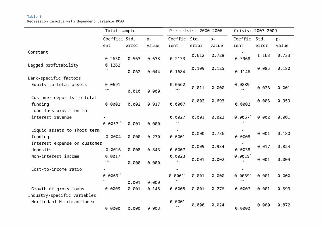
73 Appendices

variables (equity-to-asset ratio and lagged profitability) up from two lags is used. The variables in brackets after the ‘ivstykle’ command are not instrumented but are used in observed values without transformation. Note that the command small generates the t-statistics instead of z-statistics and that the option orthogonal tells the program to use the forward orthogonal deviations instead of the first differences as instruments. Robust is included in the command to generate the Windmeijer adjusted standard errors in the two-step estimator. Finally, the straightforward command twostep gives the two-step System GMM results instead of the one-step results.

Table 11 Calculations of mean differences between the subsamples

Difference in mean

Standard error comb

Satterth-waite d.f.

T-statistic

P-value

Dependent variable Return on average assets 0.2034 0.0436 1043.21 4.66 0.000

Bank-specific variablesEquity to total assets -0.3750 0.1527 1644.60 -2.46 0.014Customer deposits/ funding -1.4843 1.2032 1783.92 -1.23 0.218Loan loss provision -8.8872 1.9250 1055.28 -4.62 0.000Liquid assets to deposits 2.7098 3.0931 1789.60 0.88 0.381Interest expense deposits 0.0036 0.1329 1672.64 0.03 0.978Non-interest income 2.0007 2.2889 1025.03 0.87 0.382Cost-to-income ratio -0.4919 1.2746 1191.96 -0.39 0.700Growth of loans 0.9219 2.1822 1472.20 0.42 0.673

Industry-specific variablesHerfindahl-Hischman index -59.8380 17.0292 1900.97 -3.51 0.001Logarithm of total assets -0.0960 0.0990 1696.22 -0.97 0.332Dummy stakeholder -0.0855 0.0214 1809.29 -3.99 0.000Dummy government -0.0001 0.0115 1852.52 -0.01 0.992

Macroeconomic variablesReal GDP growth 2.8297 0.1175 1181.30 24.08 0.000Effective tax rate 1.7999 2.4693 1665.91 0.73 0.466Term structure interest 0.6257 0.0384 1044.85 16.30 0.000

The table reports the calculation of the Welch’s test on mean differences between the pre-crisis and crisis subsample. The p-values are also presented in table 4 for the descriptive statistics.

IMPLEMENTING ROBUSTNESS CHECKS IN STATA

Furthermore, several robustness checks are performed to test whether the results from the initial two-step System GMM regression are valid explanations for the true unobserved coefficients. Chapter six already mentioned that the robustness checks either relate to an adaption of the sample or to a change in the regression method. This paragraph only elaborates the implementation of regression techniques and does not describe changes in the sample since these adaptions are rather straightforward. Besides, model 3 in table 7 is not further elaborated since the model is identically

74 Appendices

the same as described here above with the exception that the option lag(1 1) is removed in the command for Stata and hence all available lags are used for the predetermined variables.

For the first robustness check (model 1) the panel data is estimated with a pooled ordinary least squares regression. The OLS regression estimates only one equation (in contrary to the two-step System GMM) in which all data is stacked together. Pooling all the data into one simple equation implicitly assumes that the relationships are constant over time and over the cross-sectional observations (Brooks, 2008). There are some other approaches that are very similar to normal OLS but that do not assume a constant relationship between variables over time and over cross-sectional observations. These approaches are classified into fixed effects and random effects models (Baltagi, 2005). The first model eliminates the bank-specific effect (μ¿¿ i)¿ from the error item by adding dummy variables for each cross-sectional observation in the main regression. Since, this fixed effects model uses dummy variables it is often referred to as the least squares dummy variable (LSDV) estimator. In the LSDV model, the dummy variables are used as intercepts for each cross-sectional observation and may differ between cross-sections but not over time (Brooks, 2008). Note that when the number of banks is large there are many dummy coefficients to be estimated, therefore a within transformation could be used to run the fixed effects regression. The within groups transformation is mathematically the same as the LSDV method only the degrees of freedom differs; for the slope coefficients both methods produce the same results. To simplify the calculations in Stata the within-group methods is used. Besides, the other panel data technique that could be applied to the model is the random effects model. In contrary to the fixed effects model, the random effects model could incorporate time-invariant variables (such as ownership) since the time-invariant variables are not absorbed by the intercept. Under the random effects model there are some additional assumptions that should hold in order to give reliable results. The random effect model assumes that the new error item is not correlated with the explanatory variables, independent of the individual observation error item and has a constant variance. The first assumption could be tested using the Hausman test. Results for this test do not reject the null hypothesis of correlation between the unique errors and the explanatory variables. The Hausman test indicates that a random effect is preferred but since the latter two assumptions are possibly violated, this thesis opts for the fixed effects model. Moreover, the coefficients of the random effects model should be the same with OLS but more efficient only when the additional assumptions hold. Finally, the Stata commands that are used to present the model for OLS and fixed effects (within) estimation are:

Model 1: Ordinary least squaresregress roaa eqtas deptfund lossrev liqfund fundcost nonint costinc growth hhindex size stakeholder government gdp tax interest , vce(robust)

Model 2: Fixed effects modelxtreg roaa eqtas deptfund lossrev liqfund fundcost nonint costinc growth hhindex size stakeholder government gdp tax interest, fe robust

Note that the lagged dependent variable is not incorporated in the model since Roodman (2009) among others, find that fixed effects and OLS give severe bias in coefficient estimates. Incorporating

75 Appendices

the lagged dependent variable introduce a trend-stationary process in the model. The Levin-Lin-Chu test for unit root for unbalanced panel data could not reject the null hypothesis of unit root, indicating that the regression is non-stationary (p-value 0.8644). Hence, incorporating the lagged dependent variable will lead to a spurious regression (Brooks, 2008). The unit root could be deleted by first-differentiating the model and is also be done using the two-step System GMM technique.

In contrary to GMM, there are several assumptions underlying the OLS and fixed effects model, regarding the distribution of the sample that makes the coefficients Best Linear Unbiased Estimators (BLUE). The assumptions are; average of the error items equals zero E (ut )=0, constant variance of the error items (homoscedastic), errors are uncorrelated, the explanatory variables are non-stochastic (the values are determinable and repeatable with new samples) disturbances are normally distributed in the sample.

First assumption cannot be violated when constant is added to the model , which is the case in equation (i). Hence, the assumption is not violated and does not result in biased parameters. If second assumption or third assumption is violated then the parameters are still unbiased and consistent but the standard errors are wrong. In our sample it is likely that there is heteroscedasticity and autocorrelation in the error items, since this is the first place why this thesis opt for the System GMM technique anyway. Hence, for both standard errors a correction is made using the robust option to make the hypothesis rejection area more conservative. The assumption of non-stochastic explanatory variables does often not hold in economic data series (Brooks, 2008). However, violation of assumption four does not necessarily result in biased coefficients, this is only the case when there is a correlation between the explanatory variables and the error item. When the robustness checks are performed using OLS and the fixed effects model equation a correlation with the error item can be observed by incorporating the lagged profitability as discussed in the theoretical section. Hence, as already discussed, equation (i) is adapted and the variable of lagged profitability is dropped from the equation. Furthermore, the assumption of normality is also violated in the panel data of European banks. The Jarque-Bera test, skewness and kurtosis are not reported in table 4 but all three test clearly reject a normal distribution of the data. When the errors follow a non-normal distribution, the parameters are no longer BLUE (Best Linear Unbiased Estimator) since the estimates are not most efficient. Particularly, in small samples the standard errors will be biased. Finally, according to Brooks (2008) there is also a more implicit assumption underlying OLS; that the explanatory variables are uncorrelated with each other (orthogonal). Deleting an orthogonal variable would not change the coefficient estimates on the other variables. There is no indication for multicollinearity as presented by the low correlation between the independent variables in presented in table 5. The problem of multicollinearity does not affect the explanatory value of the model as a whole it only affect the coefficient estimates of the highly correlated explanatory variables.

1NOTES

Following Saunders and Cornett (2008), liquidity risk refers to the risk that an asset cannot be converted into cash or that the conversion is costly. Furthermore, they state that price risk refers to the risk that the sale price will be lower than the purchase price of an asset. Finally according to their theoretical framework, credit risk is the risk that borrowers are unable to repay the loans. 2 In general, many practitioners believe that the introduction of Basel III will shift the focus of banks more and more to retail funding. In Basel III, retail funding (i.e. customer deposits and current accounts) is thought to be more stable relatively to other sources of funding and a higher amount of these funding resources will positively influence the NSFR and LCR ratio. Furthermore, this could lead to a lower gap between loans to customers and customer deposits when banks reduce their wholesale funding reliance and return to their core banking activities.3 This thesis does not make a clear distinction between corporate governance and ownership structure, as the distinction does not alter results nor affect the research design. The term ‘governance’ can relate to the internal board structure of a firm or relate to the external structure of bondholders and shareholders (debt and equity financing), of which the latter is also captured by ownership structure (Gillan, 2006),4 The distortion of debt financing is graphically represented by equation (ii); the first two fractions reflects the return on assets (net profit margin and asset turnover) while the latter fraction, the equity multiplier, captures the financial leverage effect. The equity multiplier implies that a higher financial leverage, represented by a lower equity denominator, will lead to a higher ROE, ceteris paribus. Thus, financial leverage distorts ROE as profitability measure because an overleveraged balance sheet will likely give a higher ROE ratio.

(ii) ROE=( net incomesales× salestotalassets )× total assetstotalequity

∨ROE=ROA× total assetstotal equity

5 According to the European Central Bank (2010) ROE is an inadequate measure of profitability during times of high volatility. Banks with high ROE ratios performed particularly poor during the financial crisis (a period of high volatility) due to the need for rapid leverage adjustments. Banks with high ROE ratios tend to have a low equity base, which is highly unfavorable in times of uncertainty when losses appear. According to the European Central Bank (2010) the financial crisis indicated that ROE failed to separate profitable banks from non-performing banks; thus, ROE is only a short-term measure by estimating the profitability at a particular moment in time.6 The economic value added is a concept very similar to the net present value (NPV) of an investment. In contrary to the NPV, EVA measures year to year return by calculating the difference between the cash flows on the invested funds minus the weighted cost of capital (both equity and debt financing) times total invested capital. Within the banking sector the risk-adjusted return on capital (RAROC) is commonly used to measure the profit in relationship to the risks of a bank.7 Hitherto, the theoretical chapters mentioned that regulation sets minimum capital requirements to safeguard the continuity of a bank by holding a considerable amount of Tier 1 and Tier 2 capital, also referred to as the capitalization of a bank. The capitalization of a bank is calculated on a risk-weighted basis, the amount of capital (equity for regulatory purposes) is divided by the risk-weighted assets of a bank. Hence, the term capitalization differs from the leverage structure (that is the inverse of the equity-to-asset ratio; an risk-independent metric). Since data on the equity-to-asset ratio is publicly available for all banks this ratio is used instead of the regulatory ratios that are not available for every bank for the whole period.8 A higher capital ratio can be a signal of better profitability because weaker banks cannot afford to hold the same equity without further deteriorating their earnings. Secondly, higher capital ratios lower the costs of financial distress, as banks can more easily absorb potential shortfalls and losses.9 Derivatives are excluded from total funding as these are mainly used for hedging purposes and are not a real source of funding.10 The Euro Interbank Offered Rate (EURIBOR) is often a good reference interest rate for banks. EURIBOR is the rate for which European prime banks are willing to offer term deposits to each other within the EMU zone. Since EURIBOR

interest rates are only available up to a maturity of 12-months the reference yield curve for longer maturity is extrapolated from the Euro interest rate swap curve for longer maturities. This interest rate swap curve denoted in Euros is used to obtain data for the 10-years maturity. 11 Heterogeneity across banks likely interacts with the disturbance term [i.e. E (X¿u¿ )≠0], following Baltagi (2005) leading to inconsistent and biased ordinary least square estimators/ 12 According to Baltagi (2005) the disturbance term in panel data could be either a one-way or two-way error. The methodology in this analysis incorporates a one-way error disturbance terms since the analysis assumes that there is no time-specific error but only a cross-sectional error relating to the unobserved characteristics between banks.13 An additional assumption of the System GMM estimator is that the correlation between the error item and the explanatory variables in levels is constant over time (Roodman, 2009).14 Orthogonal deviations subtract the average of all future available observations of a contemporaneous one as instrument instead of subtracting the previous observation of a variable. System GMM only holds under the assumption that changes in the instrumental variables (the transformed variables) are uncorrelated with the fixed effect (Roodman, 2009).15 Traditionally, the German banking sector is organized into a three-pillar structure in which public sector banks (‘Sparkasse’ and ‘Landesbanken’), co-operative banks and commercial banks operate in the same sector. The public sector banks and co-operative banks are mostly separate legal entities with an umbrella organization or brand. Nevertheless, the financial accounts of these banks are not consolidated on an aggregate level. Thus, this analysis does only take into account banks with total assets exceeding EUR 10 billion to avoid the inclusion of many small and similar German banks.16The interquartile range and z-score method indicate outliers whenever an observation outranges a predefined interval. The z-score method indicates an observation as an outlier whenever the z-score (observation minus the mean, divided by the standard deviation) is larger than three. The interquartile range method indicate outliers whenever the observations is beyond one point five or three times the interquartile range minus quartile one or plus quartile three. The interquartile range is defined as quartile three minus quartile one. 17 In contrary to García-Herrero et al. (2009) observations are not deleted when they are indicated by the z-score method or when observations are within the 1st or 99th percentiles. Deleting these observations will improve the explanatory value of the model and giving more significant results but the findings are not necessarily representative for the sample, it merely reflect the mean population. 18 The collapse option could be used to limit the instrumental matrix, which is quartic to T (Roodman, 2008), as calculated by the Stata software. This option prevents Stata to overestimate the model when the number of instruments is larger than the number of banks, preventing the instrument proliferation bias. However, using the collapse option will reduce the efficiency of the model. Therefore this thesis prefers to reduce the number of lags. 19 Note that in the coding process the banks that received government support are not tracked as government owned banks, incorporating these banks probably result in a significant negative coefficient during the crisis. Namely, the bad performing banks are most likely to be supported by capital injections from the government. 20 The positive parameter by García-Herrero et al. (2009) is found in China. In this country, the banking sector is likely to be more regulated; bank growth probably lead to extra costs hereby lowering the profitability.21 The exploratory conclusion is further strengthened by the opinion of several individuals that banks are too powerful in today’s economy. Increasing concentration would lead to undesirable outcomes that probably give rise to an increase in political costs.

determinants of banks profitability - erasmus university ... s. van (302984... · web viewii 11...

Documents