1

DETECTION OF SURFACE WAVES IN THE GROUND USING AN

ACOUSTIC METHOD

A Thesis Presented to

The Academic Faculty

By

Fabien Codron

In Partial Fulfillment of the Requirements for the Degree

Master of Science in Mechanical Engineering

Georgia Institute of Technology July 2000

2

DETECTION OF SURFACE WAVES IN THE GROUND USING AN

ACOUSTIC METHOD

Approved:

______________________________

Peter H. Rogers

______________________________ Waymond R. Scott

______________________________ Yves Berthelot Date Approved

_________________

3

ACKNOWLEDGEMENT

This work was accomplished in an environment very new to me. I had to

adapt to the language, the culture, and discover the campus, the city and the

people. Many people helped me go through this experience. Their knowledge,

their advice and their support made my research easier. I would like to thank

them all.

First, my advisor P. Rogers for giving me the opportunity to contribute to

this research.

W. Scott for managing the landmine detection project at Georgia Tech,

and also for his very useful debugging visits, and advice on electronics

Y. Berthelot for teaching me the basis on acoustic transducers and

supporting the exchange with Georgia Tech Lorraine.

J. Martin for his availability, his everyday advice and teaching. His

contribution to the good running of the acoustical laboratory was essential.

I would also like to thank the graduate students of the acousto-dynamic

group for their availability. They maintained a nice work environment.

4

TABLE OF CONTENTS

ACKNOWLEDGMENTS iii

LIST OF TABLES vi

LIST OF FIGURES vii

SUMMARY ix

CHAPTER

I BACKGROUND 1

A. General 1

B. An acoustic method to detect the surface waves in the ground 10

C. Litterature Review 12

II THE TRANSDUCER SYSTEM 19

A. Presentation of the Transducers 20

B. Reflection of the Ultrasonic Waves from Soil 23

C. Focusing the Transducer Sound 26

III PHASE DEMODULATION 37

A. Investigation of Digital Demodulation 42

B. Analog Demodulation 52

IV NOISE AND FILTERING 65

A. Noise Measurement 65

B. Acoustic Noise 66

C. Electromagnetic Cross Talk 67

5

D. Source Noise 68

E. Filtering 73

F. Digital Signal Processing 76

V CONCLUSIONS 79

VI RECOMMENDATIONS 82

VIII APPENDICES 85

VII REFERENCES 93

6

LIST OF FIGURES

Page

Figure 1.1 - Schematic diagram of acousto-electromagnetic experimental system 3

Figure 1.2 - Top view of the experimental system 4

Figure 1.3 - Two dimensional finite difference model 7

Figure 1.4. - Numerical model results for the mine interaction with surface wave 8

Figure 1.5 -experimental and numerical results for the surface wave propagation 9

Figure 1.6 - spatial resolution 12

Figure 1.7 - Spectrum of a pure tone modulated by a sine wave 15

Figure 1.8 - schematic of the waves phases 15

Figure 1.9 -schematic of the phase demodulation signal processing 17

Figure 1.10 - Phase demodulation for a small amplitude modulation and signal in

quadrature 18

Figure 2.1 - Schematic of the transducer assembly 20

Figure 2.2 - Cross section of a transducer 21

Figure 2.3 - Generation of the transducer signal 22

Figure 2.4 - Transmit response of the capacitance transducer 22

Figure 2.5 - Picture of transducer facing a sand sample 24

Figure 2.6 - Graph of the pressure on axis, in the nearfield 27

Figure 2.7 - sound field generated by piston at 50kHz 29

Figure 2.8 - on axis pressure generated by a 50kHz spherically focused transducer

31

7

Figure 2.9 - pressure field generated by a 50kHz spherically focused transducer

32

Figure 2.10 On axis pressure generated by a 200kHz spherically focused

transducer 33

Figure 2.11 - Normalized pressure maximums versus true focusing distance for

50, 100 and 200 kHz focused transducers 33

Figure 2.12 - Cross-section of a spherically focused transducer 34

Figure 3.1 - influence of the transducer axis angle on sensitivity 38

Figure 3.2 - Square wave with jittered edges 42

Figure 3.3 - Schematic of bit coding 43

Figure3.4 - Fourier transform of the 50kHz pure tone acquired 44

Figure 3.5 - Fourier transform of the digitized signal coded on 32 bits 47

Figure 3.6 - Fourier transform of an ideally sampled signal coded on 12bits 47

Figure 3.7 - Fourier transform of a ideally sampled signal coded on 16bits 48

Figure 3.8 - Fourier transform of signal sampled with 5.10-8s jitter 49

Figure 3.9 - Fourier transform of signal sampled with 5.10-9s jitter 50

Figure 3.10 Measurement setup 53

Figure 3.11- Picture of the transducer facing the sound projector 54

Figure 3.12 Schematic of the signal processing 62

Figure 3.13 - Operational amplifier circuit for quadrature 63

Figure 4.1 - Spectral density of a pure tone 69

Figure - 4.2 three stages passive low pass filter 71

Figure - 4.3 One stage of the Chebyshev active low pass filter 74

Figure - 4.4 Amplitude response of the active filter implemented on board 75

8

Figure 4.5 LabView diagram of the digital signal processing 77

9

LIST OF TABLES

Page

Table 1.1 - acoustic waves velocities in sand and mines 6

Table 2.1 - received signal level and signal to noise ration 25

Table 3.1 - results of the mixer test 57

Table 3.2 - Transfer function of the K-H 3 poles Bessel filter for fc=3000Hz 58

Table 3.3 - Calibration results for the TM3 configuration 60

Table 3.4 - Calibration results for the AD534 configuration 60

Table 3.5 - Results for the AD630 configuration 60

Table 4.1 - Noise floor levels in dBm after filtering of the multiplier output 72

Table 4.2 - values of the resistors and capacitors for the filter 74

10

SUMMARY

Land mine detection techniques currently in use are not reliable for

modern plastic mines. An acousto-electromagnetic technique that has the

potential to detect such mines is being investigated at Georgia Tech. It uses an

acoustic source for generating waves in the ground, which are detected with a

radar, which scans the surface to be cleared of mines. The radar system visualizes

the surface wave and its interaction with the mine by measuring the surface

vibration. This radar ground vibration measuring system is expensive and may

not be effective in all environments.

The purpose of this thesis is to investigate an ultrasonic vibrometer that

could be used to supplement the radar or replace it. An ultrasonic system was

implemented and tested with several different demodulation techniques.

Emphasis was laid on getting a sensitivity of 1-nanometer, equal to that of the

radar sensor. In order to obtain such sensitivity , design and optimization of the

source, the transducer signal, the electronic filtering and the demodulation were

conducted. The focusing of the ultrasound and the effects of spot size were also

considered.

The system presented in this thesis has good potential characteristics for

surface waves detection at a low cost. It achieves the required resolution with

transducers running at 50kHz for a vibration of the soil in the frequency range

400-1200Hz. Placing the transducers a couple inches away from the vibrating

surface produces a satisfactory spot size

11

CHAPTER I

BACKGROUND

General

Landmines are responsible for over 20,000 injuries or deaths per year.

The recent Ottawa convention banning land mines has not been signed by all the

major parties. Moreover, it does little to clean up the existing worldwide scourge

of buried land mines. According to the United Nations, more than 100 million

mines are buried over the planet. At the current rate of detection and removal,

clearing the world’s land mines could take hundreds of years.

The main problem for mine detection lies in the design of modern mines.

A mine’s structure includes a casing, explosive materials and a firing mechanism.

Most modern mines are manufactured with plastic casings. The only metallic part

is the small firing mechanism. Unfortunately, conventional metal detectors

cannot discriminate between tin cans, bullets, and scrap metal, and the firing

mechanism of a landmine. As a result, metal detectors have a considerable rate of

false alarms. What is needed is a safe, reliable and cost effective technology for

finding land mines.

As the metal part of the mine is very small, many researchers have turned

to the development of techniques detecting other properties of landmines.

Nuclear quadrupole resonance [1] has been used successfully to detect explosive

materials. By probing the earth with radio-frequency signals, this technique can

generate a coherent signal unique to certain compounds- including explosives

such as RDX or TNT. Others tried to detect the plastic casing. Electro-quasistatic

12

[2] was developed and has the potential to detect the size and the shape of plastic

objects. Many researchers have investigated acoustic techniques. The acoustic

properties of the mines are very different from those of the surrounding soil

regardless of the material used for the casing. Furthermore, the air trapped inside

the complex structure of a mine creates a cavity. This cavity is likely to resonate

at some frequencies when an external force is applied. Some effort has been

directed at the development of pulse-echo techniques [3]. Generally these

techniques did not solve the false alarm issue. Clutter, debris, rocks can also have

acoustical properties very different from the soil too. They can reflect the

pressure wave and have a signature similar to a mine’s [4].

A new land mine detection that simultaneously uses both electromagnetic

and acoustic waves in a synergistic manner is currently being investigated at

Georgia Tech [5]. This combined technique has the potential to enhance the

signature of the mine with respect to the clutter and make it possible to detect a

mine when other methods fail. This technique is presented in detail as it

motivated this thesis work. It has detected mines buried as deep as 12 inches. It

has also performed successfully in the presence of clutter and when the ground

was covered by vegetation (pine straw)

13

Figure 1.1 Schematic diagram of acousto-electromagnetic experimental

system [7]

The configuration of the system consists of a radar and an seismic-

acoustic source (electromagnetic shaker). The acoustic source induces an elastic

seismic wave into the earth, which propagates along the surface of the soil. The

elastic wave causes both the mine and the surface to be displaced. The

displacement of the mine is different from that of earth, because the acoustic

properties of the mine are quite different from those of the earth. Hence the

displacement of the surface of the soil is affected by the presence of the mine.

Resonance, scattering, and distortion of the surface wave corresponding to the

presence of a mine can be observed by visualization of the surface wave

propagation. In the current system, the electromagnetic radar is used to detect

displacements of the surface and, hence visualize the surface waves.

14

The experimental set-up [6] consists of a concrete tank filled with sand

(figure 1.2). Acoustic waves are generated using an electro-dynamic shaker

mounted upside down and equipped with a foot contacting the sand. The radar is

attached to an x-y positioner, located on a frame 50cm above the sand. The

positioner scans the radar mechanically over a 120cm by 80cm surface of sand

located in front of the shaker. Each point on the sand surface interrogated by the

radar, is exited by an identical acoustic wave and the displacement of the soil is

recorded. From this data, color animations of the surface wave propagating can

be created, which display the wave interaction with the mine.

Figure 1.2 the experimental system[8]

The tank is filled with 50 tons of damp sand with a relatively uniform

density and cohesion. The source is located at one end and radiates into a nearly

free field. The tank dimensions (figure 1.2) are large enough so that the waves

that are incident on the sidewalls do not cross the measurement region until after

15

the relevant signal have been recorded. Hence reflection on the walls does not

appear on the data recorded. Due to the large dimensions, cavity resonances are at

low frequencies in the tank.

The x-y positioner used to move the radar over the surface of the sand is

under computer control. The mechanical scanning and the recording of the data

are performed automatically. The scan is performed on a rectangular grid of

discrete positions. The points are spaced every 1cm in the x direction and every 2

centimeter in the y direction. It currently takes 24 to 48 hours to perform a

complete scan. The reason is that the measurement setup is designed to get the

maximum data quality without concern about the scan time. This time can be

greatly reduced by radar so that it can scan several points simultaneously.

There were two main challenges for the design of such a radar vibrometer.

First, make it sufficiently sensitive to be able to detect small vibrations. Secondly,

make the spot size sufficiently small. Measured vibration of the sand were

usually smaller than a micrometer. Currently the radar configuration is able to

detect 1-nanometer vibration amplitude. Such sensitivity has given a satisfactory

vertical resolution. The spot size i.e. the area illuminated by the radar must be

smaller than one half of the wavelength of the highest frequency ground wave.

Currently a small spot size is obtained by using an open-ended wave-guide as the

antenna for the radar. This antenna gives satisfactory results when its open end is

placed within a few centimeters of the surface.

Validity of the media:

Sand was chosen as the soil medium for several different reasons. It is

much easier to repeatably bury and dig up mines and clutter in sand. It also has

16

similar mechanical properties (wave velocities and displacement amplitude) to

typical unconsolidated soils when used wet and compacted. As a result, a special

device had to be installed to compensate for the evaporation of the water in the

sand close to the surface. The table 1.1 gives acoustic properties representative of

the damped compacted sand and compares them with those of a plastic mine.

These figures were used in the numerical model exposed in the next section.

Sand Typical plastic mine

Pressure wave velocities (m/s) 250 2700

Shear wave velocities (m/s) 87 1100

Table 1.1 acoustic waves velocities in sand and mines [9]

Elastic waves – land mine interaction

In order to get a better understanding of the interaction of the plastic

mines and elastic wave propagating in the ground, a numerical model was built

[9]. It consists of a finite-difference method and uses equation of motion and the

stress strain-relation. From these equations, a first order stress-velocity

formulation is obtained. A free boundary limits the top of the discretized volume

and a perfectly matched layer absorbs the outward going wave in all other

directions.

17

Figure 1.3 Two dimensional finite difference model [9]

Two simple models for antipersonnel mines were investigated: one

containing an air filled chamber and one without an air filled chamber. The

excitation producing the ground waves is a differentiated Gaussian pulse with a

center frequency of 800Hz. The figure next page shows the results of a

simulation for a mine with air cavity. The source is located at x=0 cm and the

mine at 45cm, 2cm underneath the surface of the ground. They show that the

waves hitting the mine are partially transmitted and partially reflected. This

reflection is clearly seen for the mine without air filling. For the other mine, the

reflected waves are only weakly dispersed. However, in this case, a resonance of

the mine occurs. Both of these phenomena give the mine signature.

18

Figure1.4. Numerical model results for the mine interaction with surface

waves[9]

19

Comparison with experimental model

The results computed with the finite difference model were compared to

the experimental model. They are in fairly good agreement[6] (see figure 1.5 ).

Figure 1.5 experimental and numerical results for the surface wave

propagation [7]

20

AN ACOUSTIC METHOD TO DETECT THE SURFACE WAVES IN THE

GROUND

A few aspects of the radar system are impractical. The radar has to be

very close to the ground in order to get a high signal level and a small spot size.

This is not practical for a use in fields with vegetation and soil irregularities. It is

also heavy and big and so, difficult to scan mechanically over the soil.

Cost is also an issue. Most of the countries affected by the land mine

problem are poor. Angola, Mozambique, Croatia, Afghanistan, and Cambodia

cannot afford expensive techniques. Unfortunately it seems that a radar scan is

bound to be expensive: Due to the cost of a single radar unit, it will not be

possible to use a large array of them. Therefore, it will be difficult to get a scan

time under 5 minutes for a square meter surface. Moreover, the electronics

processing the demodulation are expensive due to the high performance required

and the high frequencies of the signal.

On the other hand an acoustic device using ultrasonic waves between

50kHz and 200kHz could replace the radar sensor. The wavelength of airborne

sound waves at these frequencies would be smaller than the radar’s because of

the difference of propagation speed of electromagnetic wave and sound waves.

The transducers could be located at a reasonable distance from the ground and

easily scanned due to their small weight and size. Because they are running at

much lower frequencies, the electronics and the transducers are commercially

available and a lot cheaper.

21

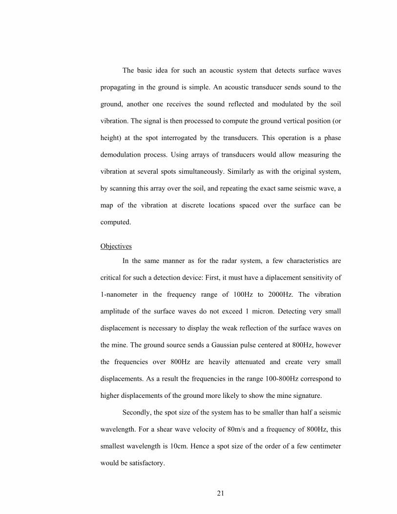
The basic idea for such an acoustic system that detects surface waves

propagating in the ground is simple. An acoustic transducer sends sound to the

ground, another one receives the sound reflected and modulated by the soil

vibration. The signal is then processed to compute the ground vertical position (or

height) at the spot interrogated by the transducers. This operation is a phase

demodulation process. Using arrays of transducers would allow measuring the

vibration at several spots simultaneously. Similarly as with the original system,

by scanning this array over the soil, and repeating the exact same seismic wave, a

map of the vibration at discrete locations spaced over the surface can be

computed.

Objectives

In the same manner as for the radar system, a few characteristics are

critical for such a detection device: First, it must have a diplacement sensitivity of

1-nanometer in the frequency range of 100Hz to 2000Hz. The vibration

amplitude of the surface waves do not exceed 1 micron. Detecting very small

displacement is necessary to display the weak reflection of the surface waves on

the mine. The ground source sends a Gaussian pulse centered at 800Hz, however

the frequencies over 800Hz are heavily attenuated and create very small

displacements. As a result the frequencies in the range 100-800Hz correspond to

higher displacements of the ground more likely to show the mine signature.

Secondly, the spot size of the system has to be smaller than half a seismic

wavelength. For a shear wave velocity of 80m/s and a frequency of 800Hz, this

smallest wavelength is 10cm. Hence a spot size of the order of a few centimeter

would be satisfactory.

22

LITERATURE REVIEW

Other active acoustic devices for detecting vibrations have been

developed in the past. In particular M. Cox and P. Rogers implemented an

underwater ultrasonic system measuring vibrations of fish hearing organs [10].

Though running underwater at very high frequencies, this system has a lot in

common with an aeroacoustic soil vibration detector. The system used a 10Mhz

source as a carrier and measured the sound reflected by the organ of the fish. The

spectral analysis of these echoes provides the frequency and the amplitude of the

organ vibration. The system was capable of measuring displacements of 1.2-

nanometer with a spatial resolution of 0.28mm. This extremely small spot size

was achieved by using high frequency focused transducers.

By crossing the transducer axis with an angle of 20 degrees, vertical axial

resolution z of 0.8mm and lateral resolution r of 0.14mm were achieved.

Figure1.6 spatial resolution

23

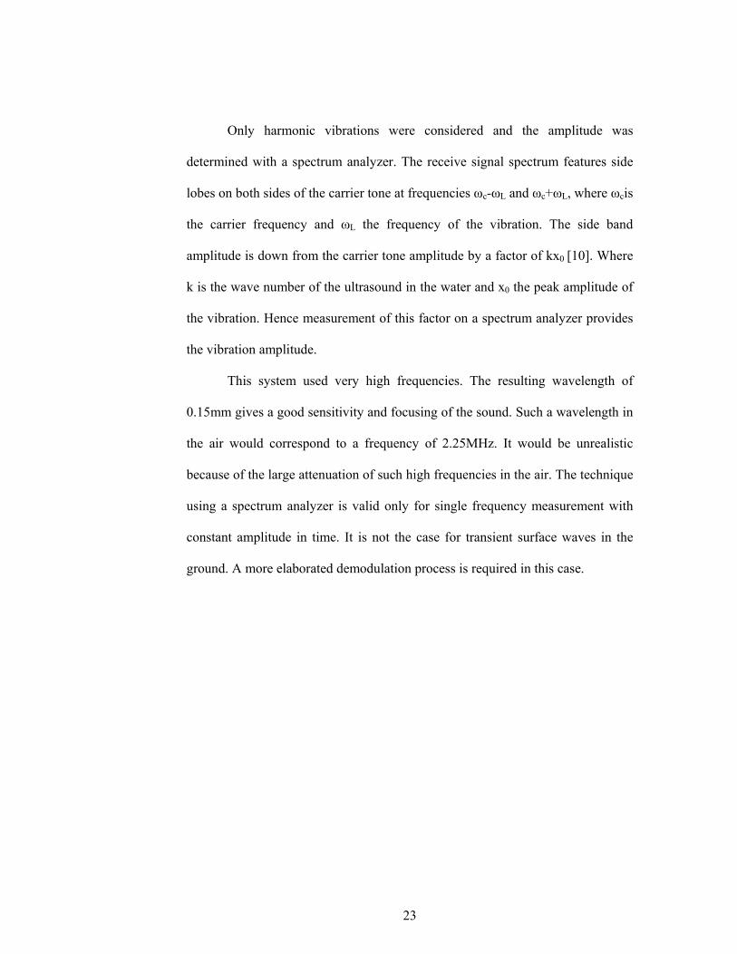
Only harmonic vibrations were considered and the amplitude was

determined with a spectrum analyzer. The receive signal spectrum features side

lobes on both sides of the carrier tone at frequencies ωc-ωL and ωc+ωL, where ωcis

the carrier frequency and ωL the frequency of the vibration. The side band

amplitude is down from the carrier tone amplitude by a factor of kx0 [10]. Where

k is the wave number of the ultrasound in the water and x0 the peak amplitude of

the vibration. Hence measurement of this factor on a spectrum analyzer provides

the vibration amplitude.

This system used very high frequencies. The resulting wavelength of

0.15mm gives a good sensitivity and focusing of the sound. Such a wavelength in

the air would correspond to a frequency of 2.25MHz. It would be unrealistic

because of the large attenuation of such high frequencies in the air. The technique

using a spectrum analyzer is valid only for single frequency measurement with

constant amplitude in time. It is not the case for transient surface waves in the

ground. A more elaborated demodulation process is required in this case.

24

Frequency demodulation techniques

Frequency modulation techniques find their origin in the last decade of

the 19th century. They were developed intensively after 1930 for communication

systems. The fundamentals of frequency demodulation are summarized in “High

performance frequency demodulation” [11] This section describes the concepts of

any phase demodulation process.

Frequency modulated signals can be represented by the following

expression:

s(t) = Acos(ωct + ϕ(t))

A denotes the carrier amplitude and ωc the carrier frequency (in rad/s).

The information carried by the signal lies in the phase ϕ(t). Frequency

demodulators process the signal in order to obtain dϕ(t)/dt.

Spectrum for sinusoidal modulation

Assume that the signal is given by

ϕ(t) = B sin(ωLt)

then s(t) = Acos( ωct + B sin(ωlt) )

The spectrum is obtained by Fourier transformation of s(t). This spectrum

correspond to the Fourier series expansion:

∑ +=n

Lc )tncos(BJn A s(t) ωω

where Jn denote the Bessel function of the first kind and order n.

For small modulation amplitudes (modulation indices), one can consider

only the first few terms. Then the spectrum basically consists of a component at

25

the fundamental frequency ωc, equal to AJ0(A) and the first harmonic

components at ωl equal to

AJ+/-1(B) ≈ .5AB

Figure 1.7. Spectrum of a pure tone modulated by a sine wave

Figure 1.8 schematic of the waves phases [11]

ωc ωc+ωL ωc-ωL ωc+2ωL ωc-2ωL

.5AB

A amplitude

Frequency

26

What demodulation technique is appropriate depends on the carrier

frequency, the amplitude and the bandwidth of the modulation, and the noise

level tolerable.

General algorithm for a phase demodulation:

A phase demodulator determines the phase difference that exists between

the two waves applied to its both inputs; the wave subjected to demodulation s(t)

and a reference wave sr(t). These waves can be noted

s(t) = A cosφ(t)

sr(t) = Arcosφr(t)

The output of the phase demodulator is:

yout = K∆Φout = Φ(t) - Φr(t)

If sr’ is the wave in quadrature with the reference wave, sr and sr’ define a

frame of reference rotating around the origin a with angular velocity ∂Φr(t)/∂t

.The phase difference can be expressed in terms of the coordinates I(t) and Q(t),

the coordinates of s(t) with respect to the rotating axis through sr and sr’. (see

picture above).

The components I(t) and Q(t) may be written as

I(t) = s . sr

= AcosΦ(t) ArcosΦr(t) + AsinΦ(t) ArsinΦr(t)

= AAr cos( Φ(t)-Φr(t) )

27

Q(t) = s . sr’

= AsinΦ(t) ArcosΦr(t) - AcosΦ(t) ArsinΦr(t)

= AAr sin( Φ(t)-Φr(t) )

The phase difference between s and the reference wave sr can therefore be

expressed as

Arctan( Q(t)/I(t) ) when I(t) > 0

Arctan( Q(t)/I(t) ) + π when I(t) < 0 , Q(t) > 0

Arctan(Q(t)/I(t) ) - π when I(t) < 0 , Q(t) < 0

Elimination of the Addition

When the bandwidth of s(t) and sr(t) is significantly smaller than their

carrier frequency, I(t) and Q(t) can be obtained by one multiplication followed by

low pass filtering, instead of two multiplication and a summation.[9]

Figure 1.9 schematic of the phase demodulation signal processing [11]

28

Elimination of the Arctan and Division

In many cases, the phase difference, Φ(t)-Φr(t), is relatively small, ie

considerably smaller than one radian. In that case, I(t) and Q(t) may be

approximated as

I(t) ≈ AAr

Q(t) ≈ AAr[Φ(t)-Φr(t) ]

Under the same conditions, the arctan-function may be approximated by

its first order Taylor term x. Therefore, the entire phase demodulation algorithm

can in this case be reduced to the determination of Q(t). The demodulator is

depicted below.

Figure 1.10 Phase demodulation for a small amplitude modulation and

signal in quadrature [11]

The amplitude of the signals A and Ar are known, so the phase difference

can be computed easily from the output of the demodulator:

r

out

AA∆Φ

=∆Φ

29

CHAPTER II

THE TRANSDUCER SYSTEM

There are several parameters to consider in choosing of the ultrasonic

transducers:

The frequency: The smaller the wavelength of the sound, the bigger the

modulation amplitude of the received signal, hence the more sensitive the system

as will be shown in chapter III. To vibration of the ground, a smaller wavelength

will give a bigger modulation of the carrier and hence, the sensitivity is increased.

However in order to get a good sound reflection from an irregular soil surface

and get a good penetration through vegetation, a longer wavelength is preferable.

The attenuation of sound in air is higher for higher frequencies. This could cause

a low signal level at the receiver, especially if the transducers are located

relatively far from the ground. At 200kHz, attenuation is a few dB per meter,

depending on the temperature and humidity of the air. Since the attenuation

increases with the square of the frequency, higher frequencies should be avoided.

At 200kHz the wavelength is 1.7mm. The sound beam will reflect correctly for

surfaces with irregularities smaller than the wavelength.

The transducer type: At ultrasonic frequencies, piezoelectric, electrostatic

and moving coil transducers can be used. All of them can create a loud sound if

designed properly. The external shape of a piezoelectric material can be design to

30

create a focused transducer. This characteristic is desirable to minimize the spot

size of the system. Piezoelectric transducers have usually a lower receive

sensitivity than electrostatic transducers. However, the better focusing would

probably compensate the loss in signal level resulting from this lower sensitivity.

Presentation of the transducers

The transducers used in the acoustic system are electrostatic (capacitance)

devices which resonate at 50kHz. They were manufactured by B&K and are

normally used for echo ranging in photography. They were chosen for their high

transmitting source level and very high receiving sensitivity (receiving sensitivity

of –45dB re 1V/Pa at 50kHz for a bias voltage of 150V). At 50kHz, the

wavelength of airborne waves is 6.8mm, i.e. four times smaller than the 8GHz

electromagnetic waves of the radar sensor. This wavelength difference insures a

gain in sensitivity of 12dB relative to the radar system and for the same signal

processing resolution. The transducers can give a spot size of a square centimeter

when located a couple inches away from the soil.

Figure 2.1 Schematic of the transducer assembly [12]

31

Figure 2.2 Cross section of a transducer [12]

The transducers require a DC bias voltage (up to 200V) and an additional

AC voltage is creates the sound (peak amplitude up to the DC bias voltage). A

thin foil is the moving surface that transforms electrical energy into acoustic

energy, and, conversely, when operated as a receiver transforms the sound wave

into electrical energy. The foil is plastic (Kapton) with a conductive coating

(gold) on the front side. It is stretched over an aluminum backplate. The

backplate and the foil constitute an electrical capacitor. When charged, an

electrostatic force is exerted on the foil. This creates a displacement of the foil

that is suspended over concentric grooves on the backplate. The AC voltage

forces the foil to move at the same frequency and to emit sound waves.

32

Figure 2.3 Generation of the transducer signal

Figure 2.4 .Transmit response of the capacitance transducer at 1meter [12]

The transducers can produce a reasonably loud sound in the frequency

range 20kHz – 100kHz with a resonance at 50kHz. Driven at 50kHz at 300Volts

peak to peak and 150Volts DC bias, they produce a sound pressure level of

approximately 118dB re 20µPa at 1meter on the axis. Measurements of the

spectrum of the signal at the receiver between 48kHz and 52Kz did not show any

noise above -130dBm when the transmitter was off. The level of the 50kHz

signal when the source is on was about 500mV. Hence this signal level was

higher than any acoustic noise in the room by over120dB.

Amplifier

150V DC Bias

Transmitter Receiver

Preamplifier

Signal Processing

50kHz generator

115dB

33

Reflection of the ultrasonic waves from soil

In the vibration experiments presented in the following chapters, the

transducers were aimed at an underwater sound projector piston. The metallic

surface of the piston is covered by a seal for underwater use. Acoustically, (in air)

it is a rigid surface. For these results to be applicable in an in situ use, the soil

must be a good reflector. In order to determine whether this is a problem, a short

experiment was conducted. It consisted in analyzing the received signal for

different reflective surfaces.

Three different surfaces were tested: A rigid surface, a sample of sand

and, a sample of Georgia’s clay soil. The rigid surface used for the test was a

wooden panel, 5mm thick, with a smooth and flat surface. It intended to set a

reference for signal level and purity. The sand sample was taken from the sand

filling the tank of the experimental mine detection set up. It was used in the same

conditions as in the tank, wet and compacted. The sample of clay was taken from

the campus grounds at a depth of a few centimeters. Both samples were 10mm

thick and had a flat top surface after being compacted with a wooden board.

34

Experiment configuration:

The transmitter was run with a DC bias of 150Volts and an AC voltage of

150Vpeak. The transducers were located 50mm away from the sample, distance

at which they focus naturally. The surfaces to be tested were placed at the same

height without moving the transducer set-up. For each one of the tests, the

received signal level before amplification was measured. The signal to noise ratio

of the signal was also observed on a spectrum analyzer. The 49kHz-51kHz

frequency range was explored with this apparatus with a resolution bandwidth of

3Hz.

Figure 2.5 Picture of transducer facing a sand sample

35

Surface Wooden board Compacted sand Clay

Signal level (mV) 600 500 500

Signal/noise (dB) >100 >100 >100

Table 2.1 received signal level and signal to noise ratio

The results show a very high level for signal reflected by the sand and

clay samples; only 20% less than the signal reflected by the flat and rigid wooden

board. Sand and clay seem to reflect the 50kHz sound beam in the same manner.

For the three tests, the received signal was very pure. Every time the signal to

noise ratio exceeded the range that the spectrum analyzer can measure (100dB).

Other tests performed with different samples of soil seemed to indicate that the

signal level is much more sensitive to the geometrical irregularities of the surface

than its nature. This test shows that sound at 50kHz reflects very well on flat

surfaces of sand or clay. The signal loss compared to a reflection by ideally flat

and rigid surface is of the order of 20%.

36

Focusing the transducer sound

Focusing the sound consists in generating a converging sound beam

focused on the soil surface. A similar design can be adopted for the receive beam

directivity, which will enhance the receiver sensitivity to sound coming from the

collocated focal spot of the transmitter on the surface of the soil. This

configuration would improve two characteristics of the system. First, the signal

level at the receiver would be increased. The sound beam converges, so the sound

pressure rises to a maximum at the soil’s surface. The reflected sound field

generates a higher electrical signal when hitting the receiver. The various sources

of noise: ultrasonic noise in the air, thermal noise of the electronics,

electromagnetic cross-talk etc. are not affected by the focusing. As a result, the

signal to noise ratio is increased, which is crucial for the sensitivity of the system.

The second characteristic of the system, improved by this technique, is the spot

size, which in principle can be reduced considerably. The sound converges

towards a particular point and thus the surface hit by the sound can have a much

smaller area than the transducer. This would enable the apparatus to detect higher

frequency waves in the ground and will give the system a better spatial

resolution. Some focusing techniques were studied in order to determine their

potential for the signal increase and spot size performance.

• Natural focusing

• spherically focused transducers

• mirrors focusing the sound generated by flat rigid pistons

37

Natural focusing of the electrostatic transducers

The transducers used in the experimental apparatus can be modeled as

rigid flat pistons. At 50kHz, the sound generated by this type of transducer in the

far field has a (–3dB) beam of angle 10 degrees with side lobes. In the far field,

The further from the source, the lower the sound pressure level. However, closer

to the transducer, in the near field, the sound pattern is more complex. The field

on the symmetry axis is well known. The following expression for the axial

amplitude p can be derived from the Raleigh integral:

p = -2ρcv sin(( k(z2+a2)1/2-kz)/2)

Where k is the wave number of the ultrasound, ρ the density of air, c the

speed of sound in the air, a the radius of the transducer, an z the distance on the

transducer axis.

Figure 2.6 Graph of the pressure on axis, in the nearfield

0 0.02 0.04 0.06 0.08 0.1 0.120

0.2

0.4

0.6

0.8

1

1.2

1.4

1.6

1.8

2

Distance on Axis in Meter

Nor

mal

ized

Pre

ssur

e A

mpl

itude

Nor

mal

ized

pre

ssur

e am

plitu

de

38

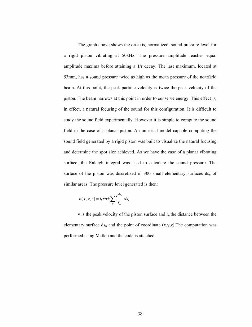
The graph above shows the on axis, normalized, sound pressure level for

a rigid piston vibrating at 50kHz. The pressure amplitude reaches equal

amplitude maxima before attaining a 1/r decay. The last maximum, located at

53mm, has a sound pressure twice as high as the mean pressure of the nearfield

beam. At this point, the peak particle velocity is twice the peak velocity of the

piston. The beam narrows at this point in order to conserve energy. This effect is,

in effect, a natural focusing of the sound for this configuration. It is difficult to

study the sound field experimentally. However it is simple to compute the sound

field in the case of a planar piston. A numerical model capable computing the

sound field generated by a rigid piston was built to visualize the natural focusing

and determine the spot size achieved. As we have the case of a planar vibrating

surface, the Raleigh integral was used to calculate the sound pressure. The

surface of the piston was discretized in 300 small elementary surfaces dsn of

similar areas. The pressure level generated is then:

∑=n

nn

ikr

dsr

ecvkizyxpn

ρ),,(

v is the peak velocity of the piston surface and rn the distance between the

elementary surface dsn and the point of coordinate (x,y,z).The computation was

performed using Matlab and the code is attached.

39

Figure 2.7 sound field generated by piston at 50kHz

As predicted, the beam narrows in the near field. It reaches it smallest

dimension at the distance 53mm, corresponding to the last axial maximum. At

this point, the 3dB spotwidth is of the order of a centimeter. This dimension is

much smaller than the 3.8 cm diameter of the transducer. When placing the

transducers at this distance from the soil’s surface the spot size would thus be

about a centimeter diameter. This is satisfactory for seismic waves of frequency

up to 4kHz. This technique does not require any investment. It was successfully

implemented on the system tested: a large increase in the signal level was

achieved. However the spot size obtained was not checked experimentally.

Note: At distances close to 53mm, interference or acoustic cross talk was

observed between the receiver and the transmitter, which led to deterioration of

the signal. A higher noise floor appears giving a signal to noise ratio inferior to

100dB.

0.05 0.1 0.15 0.20

0.005

0.01

0.015

0.02

0.025

0.03

0.035

distance on transducer axis (meter)

radi

al a

xis

dB

100

105

110

115

120

125

130

Rad

ial A

xis

(met

er)

40

Placing the transducer at its natural focusing distance improves the signal

level and reduces the spot size to a satisfactory value. However it constrains the

transducers to be at a small distance from the ground that is not very practical for

use in the fields. Therefore, investigation of more elaborated focusing techniques

was conducted. This study concentrated on getting further from the ground, and

determining the influence of frequency on the focusing.

Spherically focused transducers

In order to form an ideal focus, all the points on the transducer’s active

surface should vibrate in phase and be at the same distance of the focal point.

Such transducers are called spherically focused transducers. The vibrating surface

of a spherically focused transducer is a concave portion of a sphere centered on

the focal point. Piezoelectric transducers can be designed to exhibit this

characteristic. Even if the geometry of the transducer is perfect, the sound

focusing is limited by the wavelength of the sound waves. Sound will not focus

very well at low frequencies. In order to determine the focusing ability of such

transducers, the on-axis pressure was calculated and a numerical model was built

to display the sound field. The influences of frequency and focusing distance on

the pressure level were investigated with these tools.

The numerical model was based on the same equations as for the piston’s

sound. In this case, the vibrating surface is not planar. However, the minimum

radius of curvature of the surface considered was 50mm, which is much larger

than the maximum wavelength, used in the calculations (6.8mm). Under these

conditions, the Raleigh integral should give acceptable results.

41

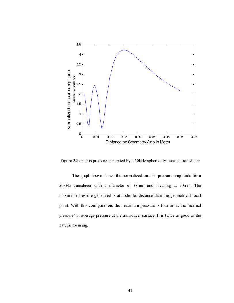
Figure 2.8 on axis pressure generated by a 50kHz spherically focused transducer

The graph above shows the normalized on-axis pressure amplitude for a

50kHz transducer with a diameter of 38mm and focusing at 50mm. The

maximum pressure generated is at a shorter distance than the geometrical focal

point. With this configuration, the maximum pressure is four times the ‘normal

pressure’ or average pressure at the transducer surface. It is twice as good as the

natural focusing.

0 0.01 0.02 0.03 0.04 0.05 0.06 0.07 0.080

0.5

1

1.5

2

2.5

3

3.5

4

4.5

Distance on Symmetry Axis in Meter

Rad

ial D

ista

nce

Nor

mal

ized

pre

ssur

e am

plitu

de

42

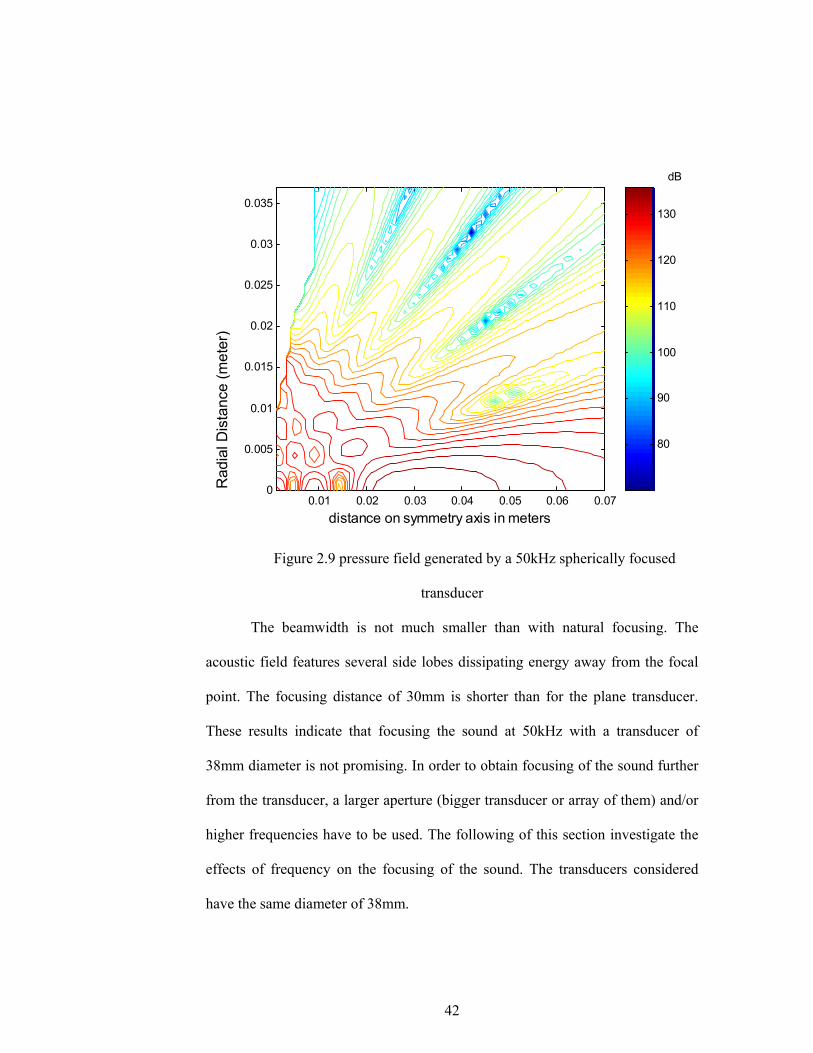
Figure 2.9 pressure field generated by a 50kHz spherically focused

transducer

The beamwidth is not much smaller than with natural focusing. The

acoustic field features several side lobes dissipating energy away from the focal

point. The focusing distance of 30mm is shorter than for the plane transducer.

These results indicate that focusing the sound at 50kHz with a transducer of

38mm diameter is not promising. In order to obtain focusing of the sound further

from the transducer, a larger aperture (bigger transducer or array of them) and/or

higher frequencies have to be used. The following of this section investigate the

effects of frequency on the focusing of the sound. The transducers considered

have the same diameter of 38mm.

0.01 0.02 0.03 0.04 0.05 0.06 0.070

0.005

0.01

0.015

0.02

0.025

0.03

0.035

distance on symmetry axis in meters

Rad

ial D

ista

nce

dB

80

90

100

110

120

130R

adia

l Dis

tanc

e (m

eter

)

43

The graphs below show the same transducer running at 200kHz. At this

frequency, the normalized pressure maximum is 13. This performance

deteriorates as try focusing further from the transducer.

Figure 2.10 On axis pressure generated by a 200kHz spherically focused

transducer

Figure 2.11 Pressure field generated by a 200kHz spherically focused

transducer

0 0.01 0.02 0.03 0.04 0.05 0.06 0.07 0.080

2

4

6

8

10

12

14

Distance on Symmetry Axis in Meter

Rad

ial D

ista

nce

Nor

mal

ized

pre

ssur

e am

plitu

de

44

The previous graph indicates as well that the focusing is a lot better at

200kHz. The sound beam concentrates very well. The side lobes are very weak

and dissipate very little energy. Higher Pressure level are reached at the focal

point, which is closer to the geometrical focal point. In order to quantify the

effect of frequency and focal distance on the focusing, the same code was

modified to compute the maximum pressure generated versus the true focusing

distance. Geometrical focusing distances where considered from 50 to 200mm

with a 5mm increment. For each focusing distance, the program calculated the

on-axis pressure determined the pressure maximum and its location and added

them to the graph. The results for three different frequencies (100,150, and

200kHz) are displayed below

Figure 2.12 Normalized pressure max vs true focusing distance at 50, 100 and

200 kHz

0.04 0.05 0.06 0.07 0.08 0.09 0.1 0.11 0.12 0.13 0.142

4

6

8

10

12

14

True Focusing Distance on Axis (meter)

Nor

mal

ized

Pre

ssur

e M

axim

um

100kHz

150kHz

200kHz

Nor

mal

ized

on

axis

pre

ssur

e m

axim

a

45

It is clearly from the graph that the focusing is dependent on the

frequency and the focusing distance. The curves exhibit a 1/r dependence on the

focusing distance. For a given focusing distance (in the frequency range

explored), the normalized pressure maximum is roughly proportional to the

frequency. It seems that to achieve a focusing 10cm or further away from the soil

surface, it would be necessary to use a carrier frequency of at least 100kHz. This

would permit a focusing factor of four. Such a configuration produces a small

spot size and a high signal level. Such an elaborated focusing technique produces

a high signal level and a small spot size. However, an increase of the running

frequency of a regular transducer will produce an increase of the natural focusing

distance and spherical focusing should only be investigated if obtaining a high

signal level is difficult.

46

Conclusion

The calculation of the on axis sound of the transducers allowed

determination their natural focusing. Locating the transducer at 55mm from the

reflective surface uses this natural focusing and leads to an increase of the signal

level and a reduction of the spot size. The sound pressure level generated at this

point is twice as high as the average pressure within the beam. The beamwidth of

the sound beam at this distance is of the order of a centimeter.

A numerical model based on the Raleigh integral was built. It calculates

the sound field generated by spherically focused transducers. The results of the

computation indicates that sound does not focus well at 50kHz. A lot of energy is

dispersed and it is not possible to focus far away from the transducers. On the

other hand at higher frequencies the results are promising. At 200kHz sound can

be focused at 130mm with a signal level gain of four. In the field, the soil surface

will certainly have irregularities, obstacles, surface debris and vegetation. Under

these conditions the transducer will have to be located at least a few inches from

the soil surface. Sound waves of frequencies of 100kHz or higher would focus a

lot better than 50kHz sound. The gain in signal level due to the focusing should

not be significantly altered by the attenuation in the air. For such small distances

at 200kHz, attenuation should be less than one dB.

47

CHAPTER III

PHASE DEMODULATION:

As discussed in Chapter I, the electrical signal generated by the receiver

contains the displacement of the reflecting surface in the form of a phase

modulation of the carrier signal. Computing the soil position from this signal thus

requires a phase demodulation process. The well known demodulation processes

used for communication, are not appropriate since the phase modulation of this

signal has a very small amplitude and is therefore difficult to detect.

For simplification of the notation, t denotes the time when wave reaches

the receiver. Therefore, the wave is reflected by the soil at t-(d+δ)/c and was

emitted by the transmitter at t-2(d+δ)/c. Where d is half of the average total path

length and δ(t) is the change in acoustic path length due to the displacement of

the soil. Hence δ is the change of acoustic length on one leg, at time t2=t-d/c. The

carrier and the received signals at time t can be respectively represented by the

following expressions:

A1cos(ωct)

A2cos(ωct -2k(d+δ(t2))

Where ωc denotes the carrier frequency and k the corresponding wave

number.

48

Figure 3.1 influence of the transducer axis angle on sensitivity

The change in length of the acoustic path, 2δ(t2), is proportional to the

vertical displacement ∆(t) of the ground due to the surface wave. The figure 3.1

shows the geometry of the transducer configuration. The angle α between the

sound beam axis and the normal to the soil is constant. The relation between the

change in length of the acoustic path and the soil displacement is then:

∆(t2) = δ(t2)/cos(α)

The central operation necessary for a phase demodulation is a simple

multiplication between the received signal and the carrier:

F1 = A1cos(ωct)*A2cos(ωct - 2k(d+δ( t2))

F1 = 0.5*A1A2[ cos( 2k(d+δ( t2) ) + cos( 2ωct - 2k(d+δ( t2) ) ]

The second term corresponds to a high frequency component. It can be

filtered by a low pass filter. For the application considered, the vibration

amplitude is much smaller than a wavelength. At 50kHz the wavelength in the air

is about 7mm and the highest vibration amplitude recorded on the experimental

δ

∆

αAxis of the sound beam

Soil level at different times

Source Receiver

d

49

model was less than a micrometer. The maximum value for kδ(t) is 9x10-4. This

is very small compared to 1 radian, and a first order Taylor series is a good

approximation for the signal. After low pass filtering and this approximation, the

product of the carrier and the received signal can be written:

LF1 = 0.5*A1A2( cos(2kd)k) - 2sin(2kd)kδ( t2) )

Hence we get a signal composed of a constant term dependent of the

transducer location and a term proportional to the displacement of the soil. d is

unknown, as a result, this signal by itself cannot provide the displacement of the

ground.

A second low frequency signal can be obtain by computing a similar

multiplication of a quadrature of the carrier and the received signal :

F2= A1sin(ωct)*A2cos(ωct - 2k(d+δ( t2))

F2 = 0.5*A1A2[ sin( 2k(d+δ( t2) ) + sin( 2ωct - 2k(d+δ( t2) ) ]

After low pass filtering,

LF2 = 0.5*A1A2( sin(2kd) + 2cos(kd)kδ( t2) )

AC1 DC1

AC2DC2

50

The four terms AC1, AC2, DC1 and DC2 can be used to compute the

displacement of the ground:

DC12+DC22= 0.25A12A2

2( cos(2kd)2+sin(2kd)2 ) = 0.25 A12A2

2

AC1xDC2 = -0.5kA12A2

2sin(2kd)2xδ( t2)

AC2xDC1 = 0.5kA12A2

2cos(2kd)2xδ( t2)

And

AC2xDC1 - AC1xDC2 = 0.5kA12A2

2δ( t2)

There fore,the displacement of the ground can be computed by the

following operation:

DC1 designates the constant component of the signal, i.e. its average over

time. AC1 designates the other component of the signal.

LF1= DC(LF1) + HP(LF1)

Resolution of the demodulation:

When corresponding to the minimum amplitude harmonic signal

detectable of frequency ωL, δm(t) can be noted:

δ(t) = x0cos(ωLt)

The signal on the receiver is then

A2cos(ωct - 2kd - 2kx0cos(ωLt) )

The spectrum of this signal shows the carrier frequency ωc and peaks at

ωc+ωL and ωc-ωL. The side lobe amplitude is down to the carrier by factor of kx0.

)cos(2)2 DC (DC1 DC2AC1-DC1AC2)( 222 αk

t+

××=∆

51

For a 1-nanometer vibration amplitude and a carrier frequency of 50kHz, this

factor corresponds to the sensitivity wanted for the demodulation device.

For a 1-nanometer displacement, x0=10-9cos(α) and

kx0 = 9.24E-7

20*Log10(kx0) = -120 dB

Computation of the signal processing

The operations necessary for a phase demodulation are: quadrature, two

multiplications, low pass filtering, and additions and multiplications of low

frequency signals. These operations can be performed by different means. For the

radar system, a mixer is used to perform the multiplication of an 8GHz signals. It

is a passive device that multiplies two signals. Some of its advantages are a very

low noise level, and very high frequency operation. At low-ultrasonic frequencies

another alternative is to use an active multiplier. This device exhibits a better

linearity than a mixer and the advantages of an active chip: low output

impedance, high output level, and high input impedances. However, four

quadrant multiplier chips have an internal noise that is dependant on the quality

of the manufacturing and the design.

These operations can also be performed digitally. Many communication

systems, particularly demodulation devices, use digital technology. It provides a

very versatile tool that can perform many different operations with the same

system. The performance of digital systems is improving rapidly with computer

technology. More over, a computer has to be part of the total system anyway for

data acquisition and storage.

52

INVESTIGATION OF DIGITAL DEMODULATION

As with any other demodulation technique, the problem is that the

modulation amplitude is very small. Independent of the quality of the program

performing operations on a signal, the performance of a digital demodulation

system is limited by the data acquisition card (or component). The acquisition

card converts an analog signal into a digital signal. It performs two operations

that add noise to the input signal: sampling and coding. First it samples the signal

at regular time intervals. This operation cannot be performed without some error.

The time intervals vary slightly and the value of the signal is not taken at

perfectly regular pace. This is called the clock jitter.

Figure 3.2 Square wave with jittered edges [14]

This jitter generates noise that has a spectral content generally not

uniform over all the frequencies. The noise floor corresponding to this phase

noise is usually small compared to the signal and it can be neglected for most

applications. However, when dealing with large dynamic range, it has to be

53

considered. The noise floor level has to be lower than the smallest signal level to

be acquired by the card.

Figure 3.3 Schematic of bit coding

After sampling, the analog to digital converter card codes the amplitude

of each sample over a limited number of values. An approximation is then made:

the nearest value is taken. The user specifies a voltage range R for the input level,

the resolution of the coding is then R/2n where n is the number of bits used to

code the sample. This stage is the n-bit coding. Common A/D cards use 12 or 16

bits coding which correspond respectively to a maximum error of 0.02% and

0.0015%. The rounding process induces an additional error. In the same way as

the clock jitter, this error generates a noise that has its own spectral component.

Again, noise level due to the coding has to be lower than the smallest relevant

signal level.

Analog signal Sampling Coding

54

Test of an Analog to Digital card

To assess the capabilities of an A/D card in terms of noise floor level, a

test was performed on a recently acquired card. This card was designed and

manufactured by National Instrument and features: a sampling frequency of up to

1MHz, a 20MHz clock, 8-channel acquisition, and 12-bit coding.

The noise floor level was evaluated by computing a Fourier transform of a

signal acquired on the card. A 50kHz pure tone was generated externally with a

function generator and input to the card. The A/D card digitized the signal over a

period of 1s, at a sampling frequency of 250kHz. This data was imported to

Matlab to compute the Fourier transform. These settings give the spectral content

of the discrete signal up to 125kHz, and with a resolution of 1Hz. The results are

displayed below

Figure 3.4 Fourier transform of the 50kHz pure tone acquired

55

This graph shows:

A sharp peak corresponding to the pure input tone

A broadband noise level about 95dB down to the 50kHz tone level

Other noise peaks with amplitude level up to 30 dB above the

broadband noise floor

When input into a spectrum analyzer with a resolution of 3Hz, the signal

generated by the function generator shows a signal to noise ratio over 100dB.

Hence, we have to conclude that the origin of noise shown by the Fourier

transform is the card and the digitizing process. The desired sensitivity

corresponds to a noise floor 120 dB below the carrier. A very generous signal to

noise ratio for this card would be 95dB. This is not satisfactory. This particular

card does not have a performance suitable for the surface wave detection

application.

In order to determine the characteristics of an A/D card suitable for this

application, a further investigation was done to determine appropriate

characteristics for this device. Two programs modeling the jitter and bit coding

noise sources discussed previously were designed.

56

Bit coding model:

The noise generated by the bit coding operation was evaluated by a

Fourier transform of a digital signal. An ideal digital signal was created over a

period of one second at a sampling frequency of 250kHz and machine precision

(32 bit coding). It was then coded in 12 bits and 16 bits precision. The Fourier

transform of these 3 data vectors shows the noise floor resulting from the bit

coding. There was no clock Jitter modeled, hence the only noise results from the

32 bit coding for Matlab real numbers. This has very small effect compared to

the errors modeled by the program.

For this test a 50kHz signal modulated at 200Hz with an amplitude B of

10-6 radian was used. This modulation corresponds to a signal 15dB above the

resolution desired for the detection device.

S = cos (ωt+Bsin(400πt) )

The following expression was used to model the bit coding of a signal

.

1-n

1-n

nBits 2S) round(2S =

57

Figure 3.5 Fourier transform of the digitized signal coded on 32 bits

Figure 3.6 Fourier transform of an ideally sampled signal coded on 12bits

58

Figure 3.7 Fourier transform of a ideally sampled signal coded on 16bits

The 3 graphs above show the noise floor level in the frequency range

49kHz-51kHz, which is the relevant range for modulations up to 1kHz. The noise

floor rises as the bit coding precision decreases. The 12 and 16 bits coded signal

have respective signal to noise ratio of 115dB and 140 dB. This performance is

satisfactory for the ground wave detection device: the side lobes appear clearly.

Hence the 12 bit coding does not seem responsible for the broadband noise that

appears on the A/D card test.

59

Clock Jitter noise

In the same manner as for the bit noise, the clock jitter noise was modeled

and its effect on the broadband noise analyzed. Little information was found on

the clock jitter for the card tested and for acquisition cards in general. A model

was used to find the maximum clock jitter compatible with a good performance

for the device.

A very simple model was used for the clock jitter. Each sampling time ti

was given an error ∆ti, normally distributed and centered on the exact time. The

variance of the normal distribution was chosen to be one third of the peak jitter

amplitude Ajitter. This figure insures that 99.75% of random time errors were in

the interval [- Ajitter; Ajitter ].To each sampling time ti, was added random error ∆ti:

∆ti = AjitterN(0,1)/3

Where N(0,1) a normally distributed random number with variance 1.

7

Figure 3.8 Fourier transform of a signal sampled with 5.10-8s jitter

60

Figure 3.9 Fourier transform of a signal sampled with 5.10-9s jitter

The results show a rise of the broadband noise as the jitter increases. A

jitter amplitude of 5x10-8 second generates a noise level similar to the card tested.

This jitter would have to be reduced by a factor of more than ten to give a

performance suitable for the device (second graph). Little information was found

on a possible model for the clock jitter, so several models were tried with

different error distributions and means as well as accumulation of the error. The

results varied only slightly. Hence, it is believed that the figures above give a

good idea of the jitter amplitude. It seems a reasonable assumption that the

sampling jitter is inversely proportional to the clock speed of the acquisition card.

In this Case, a clock 50 times faster than the one on the card tested would be

satisfactory, i.e. a 1GigaHertz clock.

61

Conclusion:

The simulations seem to indicate that the factor limiting the performance

of the acquisition card tested is the clock jitter, not bit coding. Getting a signal to

noise ratio of at least 120dB requires 16bits coding and a Jitter amplitude of 10-9

second. Little information was found on the jitter of commercially available A/D

cards. However, if it is inversely proportional to the clock speed, a 1GHz clock

would be satisfactory for the surface wave detection application.

Commercially available fast A/D products with a 16-bits coding and

several acquisition channels are relatively expensive. Since digital demodulation

seems to require electronic boards approaching the limits of current digital

technology, it was decided to use an analog technique for the experimental

system of this thesis. Analog technology is more mature and specialized. Analog

chips and devices can perform demodulation operations at a low cost.

62

ANALOG DEMODULATION

An analog phase demodulation system was implemented. The system

involves a quadrature circuit, multiplication devices, active filtering and

amplification. This section discusses the processing and the tests of different

configurations.

The performance of the process dictated by the dynamic range of the

multiplication device. It has to be able to multiply signals at very different levels

(The side lobe level is much smaller than the pure tone level). In order to

determine the device most appropriate for the multiplication, a simplified

demodulation configuration was used. Quadrature of the carrier, computer

acquisition and digital processing were not implemented for these tests.

Quadrature between the received signal and the carrier was realized manually.

The transducers were moved slightly so that the length of the acoustic path

created quadrature. This was feasible thanks to the relatively large wavelength of

the ultrasonic wave. In this situation, the derivation of the multiplication becomes

F1 = A1cos(ωct) x A2cos( ωct - π/2 - 2kδ(t2) )

F1 = 0.5*A1A2[ sin( – 2kδ(t2) ) + sin( 2ωct – 2kδ(t2) ) ]

After Low pass filtering and a Taylor approximation, the signal can be expressed

by:

LF1 = A1A2 kδ(t2)

63

. As the transducers are immobile, the amplitudes of the signal A1and A2

are constant. Hence the low frequency signal is directly proportional to change in

length of the acoustic path δ(t). This configuration enables us to easily investigate

individual analog system components and remove possible noise sources and

implementation problems related to the quadrature process, the computer

acquisition and the digital processing. This configuration was used to test both

mixers and a multipliers.

Figure 3.10 Measurement setup

Multiplication

Spectrum analyzer

Preamplifiers

Low pass filter

CARRIER SIGNAL

Accelerometer Received signal

Vibrating piston

64

Test of a mixer demodulation configuration

A mixer multiplication was implemented in the system and tests were

performed in order to determine its performance. The mixer used was

manufactured by Mini-circuit and referenced ZAD 3-H. It features a high input

signal level and low noise characteristics.

A sound projector designed for underwater sound generation provided the

vibrating surface. It is an electromagnetic device actuating a flat circular piston of

100-millimeter diameter. A rubber membrane, for sealing purposes, covers the

piston. This surface is effectively rigid for a good sound reflection. It is larger

than the spot size achieved by the ultrasonic transducer, and vibrates uniformly.

Figure 3.11 Picture of the transducers facing the sound projector

The vibration amplitude was controlled with an audio amplifier according

to measurements from an accelerometer. The audio amplifier amplified the signal

produced by a Wavetek signal generator and powered the sound projector. The

intensity of the vibration could be set by either the signal generator and the

65

amplifier. The vibration amplitude was measured by an accelerometer attached to

the center of the piston surface with bee wax. The accelerometer, of sensitivity

3.42mV/g, was used with a charge amplifier and a spectrum analyzer in order to

determine the peak acceleration of the surface. From the voltage level U given in

dBm by the spectrum analyzer, the peak voltage amplitude is:

20102U

refrefpeak RV π=

Where Rref = 50Ω is the reference impedance and πref = 1mW is the

reference power. The peak acceleration in ms-2 is then

31042.38.9

−×= peakV

γ

As we consider one sinusoidal frequency, the peak amplitude of the

vibration is:

2max zωγ

=

Analysis of the spectrum of the modulated signal can provide a quality check for

the vibration amplitude measurement. The side lobe induced by the vibration are

down from the carrier amplitude by a factor of kx0, where x0 is the peak

amplitude of the vibration. Therefore the vibration amplitude calculated from the

modulated signal is:

20log

)cos(1

0carrierlobe VVA

kx −

=α

66

During the tests the transducers were located at their natural focusing

distance from the piston. They were aiming at the center of the piston from a

distance of 60mm at a total angle of 54 degrees (α = 27degrees). A Krohn-Hite

source repeater amplified the signal from the Analogic function generator to

150V peak. A Krohn-Hite active low pass filter filtered the output of the mixer. It

performed a 3-poles Bessel filtering with a –3dB cutoff frequency at 3000Hz.

The response of the system was studied for a fixed vibration amplitude between

200Hz and 1200Hz. In order to get the maximum output level, the mixer input

levels were set at the maximum specified by the manufacturer (see below).

Maximum input on LO: 17dBm (2V)

Maximum input on REF: 7dBm (700mV)

For each frequency, the vibration was set to 40 nanometers according to

the accelerometer measurement. The side lobe level was measured for the

received signal. The mixer output and the noise floor level were measured after

filtering. All the measurements were performed on the spectrum analyzer with a

resolution bandwidth of 3Hz.

From the measurements, the sensitivity of the analog demodulation was

computed. This sensitivity corresponds to the smallest modulation detectable, it is

expressed by the ratio of the of the smallest side lobe detectable to the carrier

level on the modulated signal (in dB). The value displayed in the table was

computed from the side lobe level and the signal to noise ratio at the output of the

mixer:

Demodulation sensitivity = tone level – side lobe level + output Signal/Noise

67

Freq

Accelerometer

measurement

(dBm)

Displacement

From Acc

(meter)

Side

lobe/peak

(dB)

Displacement

From side lobe

(meter)

Output

level

(dBm)

Noise

Floor

Level

S/N

(dB)

sensitivity

(dB)

200 -82.3 4.4E-08 -85 3.0E-08 -82.3 -95 12.7 97.7

400 -70.3 4.4E-08 -86.5 2.6E-08 -83.3 -98 14.7 101.2

600 -63.2 4.4E-08 -88.95 1.9E-08 -83.8 -101 17.2 106.15

800 -58.2 4.4E-08 -88.6 2.0E-08 -85.3 -101 15.7 104.3

1200 -51.2 4.4E-08 -88.35 2.1E-08 -87.8 -104 16.2 104.55

Table 3.1 results of the mixer test

Often, the two side lobes levels measured on the spectrum analyzer had different

levels by one or two dBs. This phenomenon is not yet explicable. A possible

reason is a the amplitude modulation of the signal because of the variation of the

length of the acoustic path. Such modulation appears as side lobes in the

spectrum of the modulated signal. Unlike for the case of a phase modulation, the

side lobes have the same phase. Hence, the superposition of a phase and

amplitude modulation can generate such uneven side lobes. The value in the table

above is the average of the two side lobe levels. The displacement given by the

accelerometer and the side lobe levels match pretty well. Differences could come

from the inaccuracy of the accelerometer measurements. For a constant

displacement of the piston, as the frequency is increased, the output level

decreased a little. Part of this phenomenon is due to the filter, whose cutoff

frequency is relatively close to the signals.

68

Freq 200 400 600 800 1200 Gain (dB) 0 0 -0.2 -0.6 -1.6

Table 3.2 Transfer function of the Krohn-Hite 3 poles Bessel filter for fc=3000Hz

The constant peak displacement was set according to the accelerometer signal.

The side lobe levels seem to indicate that in the lower frequency range the actual

vibration amplitude was higher. This seems to indicate that the relatively lower

sensitivity of the accelerometer at low frequencies is the second factor

responsible for an apparent drop of the output in the higher frequency range.

Due to the drop of the noise floor, the sensitivity increases with frequency. The

average resolution for the mixer demodulation and over the frequency range 200-

1200Hz is 103dB. It corresponds to a displacement amplitude of about 9 nm for a

50kHz carrier.

We can also observe a drop of the noise floor level when the frequency

increases. This could be due to the spectral impurity of the 50kHz. The side lobe

must be extracted from the skirt of the carrier. It was not possible to measure this,

since the signal to noise ratios achieved are higher than the measurement

capability of the spectrum analyzer, even for frequencies close to the carrier

frequency.

Conclusion:

An average sensitivity of 103dB was obtained over the frequency range

200-1200Hz. This is close to the desired performance. A higher noise floor level

was observed in the lower frequency range. A problem was encountered with the

69

mixer device; its low input impedance distorted the input signals. It was thus

decided to implement multiplier chips that would give high input impedances,

low output impedances and higher signal levels, rather than mixers. These

devices have also better linearity. Crystal oscillators (which have a higher

spectral purity) were bought in an attempt to reduce the noise floor level in the

low frequency range.

Sensitivity tests of multiplier demodulation configurations

Tests were performed with the same experimental setup using multiplier

circuits. A multiplier cannot be used on the radar system because the frequency is

much too high. However, these active chips can at frequencies higher than 1Mhz,

and so can perform operations around 50kHz very well. Due to their active

nature, they can provide a high input impedance, higher signal levels, and a good

linearity. Several multiplier circuits were tested. Three are presented in this

report. The circuit TM3 uses a four-quadrant multiplier designed by Analog

Devices. It accepts input levels up to 10Volts peak and an adjustable gain is

available at the output. The four-quadrant multiplier AD534 and the chip AD630

manufactured by Analog devices were also tested.

The configuration of the test was identical to the mixer test. However the

gain of the preamplifiers were increased so that the input levels are maximal.

70

Freq

Accelerometer

measurement

(dBm)

Displacement

From Acc

(meter)

Side

lobe/peak

(dB)

Displacement

From side lobe

(meter)

Output

level

(dBm)

Noise

Floor

Level

S/N

(dB)

Sensitivity

(dB)

200 -82.3 4.4E-08 -86.6 5.1E-08 -57.8 -82 24.2 110.8

400 -70.3 4.4E-08 -87.4 4.6E-08 -58.8 -88.6 29.8 117.2

600 -63.2 4.4E-08 -88.2 4.1E-08 -60 -91 31 119.2

800 -58.2 4.4E-08 -88.5 4.0E-08 -60.3 -92 31.7 120.2

1200 -51.2 4.4E-08 -89 3.8E-08 -62.8 -94 31.2 120.2

Table 3.3 Results for the TM3 configuration

Table 3.4 Results for the AD534 configuration

Table 3.5 Results for the AD630 configuration

Freq

Accelerometer

measurement

(dBm)

Displacement

From Acc

(meter)

Side

lobe/peak

(dB)

Displacement

From side lobe

(meter)

Output

level

(dBm)

Noise

Floor

Level

S/N

(dB)

Sensitivity

(dB)

200 -82.3 4.4E-08 -86.5 5.1E-08 -57.3 -83.1 25.8 112.3

400 -70.3 4.4E-08 -88.3 4.1E-08 -57.6 -92 34.4 122.7

600 -63.2 4.4E-08 -87.5 4.5E-08 -58.4 -94 35.6 123.1

800 -58.2 4.4E-08 -87.5 4.5E-08 -58.2 -95 36.8 124.3

1200 -51.2 4.4E-08 -88.1 4.2E-08 -60.4 -94 33.6 121.7

Freq

Accelerometer

measurement

(dBm)

Displacement

From Acc

(meter)

Side

lobe/peak

(dB)

Displacement

From side lobe

(meter)

Output

level

(dBm)

Noise

Floor

Level

S/N

(dB)

Sensitivity

(dB)

200 -82.3 4.4E-08 -85 6.1E-08 -57.3 -86 28.7 113.7

400 -70.3 4.4E-08 -86.5 5.1E-08 -57.6 -90 32.4 118.9

600 -63.2 4.4E-08 -87.8 4.4E-08 -58.4 -91.4 33 120.8

800 -58.2 4.4E-08 -86.3 5.2E-08 -58.2 -91 32.8 119.1

1200 -51.2 4.4E-08 -88.0 4.3E-08 -60.4 -94 33.6 121.6

71

For the three the multiplier configurations: The results show a great

increase in the sensitivity relative to mixer configuration. The objective of 120dB

resolution is reached for a large part of the frequency range. The same rise of the

noise floor is observed in the low frequency range. The AD534 multiplier seems

to give slightly higher output level and the same noise floor level as the TM3

circuit.

The configuration with one multiplication implemented for these tests is

not very realistic for a use in the fields. The distance from the transducer to the

soil surface would have to be adjusted so that it creates continual quadrature

between the receive signal and the carrier. This is not practical, especially when

using plane arrays of transducers over an irregular surface. Therefore a signal

processing that can run with an arbitrary acoustic delay (2kd) has to be

implemented. The schematic next page illustrates a possibility. This flow diagram

follows closely the derivation exposed at the beginning of the chapter. The

processing uses a quadrature circuit and two multiplier circuits in addition to the

previous configuration. The analog part of this system is presented in the

following section. The filtering and the digital operations are exposed in the next

chapter.

72

Figure 3.12 Schematic of the signal processing

The quadrature was obtained by realizing a differentiating circuit with an

operational amplifier. This differentiation gives a phase shift of π/2 to the 50kHz

carrier. The impedances of the feedback resistor and capacitor were chosen to get

a gain of 1 at 50kHz. The circuit can process carrier level up to 10Volts peak.

The analysis of the output signal on the spectrum analyzer showed a very pure

signal. The signal to noise ratio was over 100dB.

PHASE SHIFT - π/2

PREAMPLIFIERS

MULTIPLICATION

A/D

CARRIER SIGNAL

RECEIVED SIGNAL

A/D

MULTIPLICATION

LOW PASS

FILTERING

2 CHANNELS

73

R = 570 kΩ C = 5pF

Gain at 50kHz: G50kHz = 1/RCω

=.9

Figure 3.13 Operational amplifier circuit for quadrature

Tests were performed with quadrature between the carrier and the received signal

realized with this circuit. The results showed identical noise and output levels

with the results obtained by achieving quadrature by adjusting the acoustic path

length. This indicates that the performance of this circuit is suitable for the

intended application.

74

Conclusion

The feasibility of digital phase demodulation was investigated. Such

processing would require a very fast acquisition card featuring low clock jitter

and at least 16bits digitization. Due to the cost of such a device, an analog

solution was investigated. An analog phase demodulation was implemented and

tested with several multiplication devices. The tests were performed with actual

transducer signals reflected from a vibrating rigid surface. The sensitivity of the

different configurations was computed over the frequency range [200,1200Hz]

from the modulated signal and the output signal spectra. In every case, the

sensitivity was found to be poorer by a few decibels in the lower part of the

frequency range. The origin of this is a rise of the noise floor at low frequencies.

The mixer configuration performed a resolution from 98dB at 200Hz to 104dB at

800Hz. The multiplier circuits gave better results thanks to their much higher

input impedance and output levels. Sensitiviy from 110 to 120dB for the TM3

and sensitivity from 112 to 124dB was observed for the AD534 multipliers.

Finally, a quadrature device having a dynamic range over 120dB was built with

an operational amplifier.

75

CHAPTER IV

NOISE AND FILTERING

A crucial part of this thesis work was to get a good sensitivity. Very small

signals received by the transducer have to be enhanced by signal processing. Any

noise in the system will tend to hide the small desired signal. The noise in the

demodulated signal at the very end of the processing can have several origins.

This chapter intends to make a list as complete as possible of the noise sources in

the system and present the solutions implemented to reduce them. In particular,

this chapter will present the filtering techniques chosen to remove the unwanted

frequency components of the signals.

Noise measurement:

Throughout this study, noise was considered in the frequency domain.

When trying to reduce or remove it, frequency is an important parameter. A

spectrum analyzer is a very powerful tool for investigating noise. Its very high

input impedance and great sensitivity allow tracking very small signal levels and

noise floors. All the noise floor measurements stated in this report correspond to

a resolution bandwidth of 3Hz. Though very powerful, this tool is limited by its

dynamic range of 100dB. It can ‘only’ display signals that are 105 times smaller

than the highest signal level input. The sensitivity wanted for the demodulation

device is 20dB higher than this. As a result it is not possible to state that a

76

specific component of the system is good enough by direct measurement. The

spectrum analyzer can only show whether or not this signal to noise ratio exceeds

100dBt. At the end of the process, after multiplication and filtering the sensitivity

can be evaluated. However, it is difficult to determine the origin of the noise

floor.

Acoustic noise:

When implementing an acoustic method for surface wave detection, one

inevitably meets acoustic noise. The capacitance transducers function similarly to

a speaker and a microphone. A background noise in the air would be detected by

the receiver and thus becomes noise in the system. Spectral measurements were

made on the receiver signal. When the transmitter is not running, the noise floor

level around 50kHz is below –125dBm. During the operation of the system, the

signal level is about 3dBm. Therefore the available dynamic range of the air

media is at least 128dBm. Measurements of ultrasonic sound level in the lab

showed that it was not significant. The projector’s vibrating piston produces

sound under 1200Hz that is detected by the receiver. This low frequency

component of the received signal perturbs the multiplication operation. Mixers

and multipliers do not work ideally and some of the input signal feeds through

the chip. Therefore the low frequencies coming from the receiver have to be

filtered. This problem is only related to the laboratory and the calibration test.

The surface waves in the soil do not radiate sound in the air efficiently. They

generate evanescent waves and the sound level decays exponentially as the

observation point is moved away from the surface. However a high pass filtering

device should still be installed to allow use near a low frequency sound source

77

(vehicle motor running…). It is easy to implement. The capacitance receiver is

not very sensitive in this frequency range. Moreover this frequency range

(100Hz-2kHz) is located at least 5 octaves away from the carrier frequency.

Therefore a simple one or two pole passive high pass filter with Fc=30kHz can

achieve a 30 or 60dB attenuation. On the system, the SRS pre-amp used to

amplify the received signal performs this filtering.

Another noise problem related to the transducers was encountered. At

some position close to the surface, the transducers showed interference. The

signal to noise ratio on the receiver was deteriorated and showed interference

maxima and minima at several frequencies very close to each other. Placing the

transducers at their natural focusing distance from the vibrating surface solved

this problem.

Electromagnetic Cross-talk

The tests where performed in the Space Science and Technology center of

Georgia Tech. In the laboratory many power lines and forty-two 34W-fluorescent

tubes provide the light. The power line generates an electromagnetic field at

60Hz and its harmonic frequencies (120Hz, 180Hz, 240Hz... ). Similarly, the

fluorescent light generates electromagnetic noise at frequencies such as 300Hz. In

order to isolate the system from this noise, all the equipment used were shielded:

All the wire connectors used were BNC shielded cables

A brass back plate connected to the ground was added to the back

of the transducers

The multiplier circuit, the derivator circuit and the filter were

placed in metal boxes.

78

The Power line can also talk through commercially available equipment. This

problem was particularly met with the transformer supplying DC voltage to the

Op-amp and the multiplier circuits. To solve this problem, the transformers were

abandoned and batteries were placed inside the multiplier chassis.

The source:

The ‘Analogic’ digital function generator was used as a signal source. It

can generate a pure tone, with a signal to noise ratio over a 100dB. This

performance is hard to determine more accurately because most high

performance spectrum analyzers can only discriminate signals with 100dB of

amplitude difference. The modulation of the acoustic signal, generated by the

vibration, appears in the spectrum as side lobes of the pure tone. These side lobes

have frequency ωc+ ωL and ωc - ωL and amplitude kH*u/cos(α), where u is the

displacement amplitude of the ground surface. Hence, frequency ranges [ωc -

1200, ωc -100] and [ωc +100 ωc +1200] have to be clear of noise on the acoustic

signal and therefore on the source signal. That is, the noise level has to be 120dB

down from the 50kHz tone at these frequencies. In other works, the spectral

purity of the signal generator is very important. Typically, this is a problem for

frequencies close to the tone where the spectral density of the source phase noise

is the highest. In particular, it could be the reason for the higher level of the noise

floor for low frequencies on the multiplier output.

79

Figure 4.1 Spectral density of a pure tone

A test of the Analogic source with a spectrum analyzer seemed to show that the

source signal to noise ratio is voltage level dependent. At some output levels, the

source signal to noise ratio could be a little less than 100dB. Thus the signal to

noise ratio of this device was no greater than 100dB

In order to increase this to 120dB, several techniques were studied.

Voltage sources do not generate perfectly pure tones. Slight instantaneous phase

or frequency shifts create a noise floor. In the same manner slight random

variation of the amplitude will also create a noisy environment. These noise

sources are respectively called phase and amplitude noise.

Phase noise cannot be reduced easily on an existing source. However, we

can use a technique that annihilates its effect on a multiplier operation. The

random phase shift induces a broadband noise on the output of the multiplier.

This is because the phase shifts of the two inputs are not the same. The reason is

that the carrier signal comes straight from the source whereas the modulated

signal is delayed by the propagation of the acoustic wave from the transmitter to

Frequency

50kHz pure tone

Analyzer capability

Noise floor level

80

the receiver. This can be corrected by implementation of a delay line on the

carrier signal. The idea is to create a delay on the carrier signal that would equal

the acoustic propagation time. Then, the instantaneous phase shifts originated by

the source will match at the input of the multiplier. This delay can be performed

electronically, or acoustically. An acoustic delay line composed of two additional

capacitance transducers was implemented on the system. The transducers were

placed facing each other and separated by a distance equaling the acoustic path of

the two other transducers. Unfortunately, no positive change was observed on the

output of the multiplier. This indicates that the highest noise source is the system

is not phase noise from the source.

The broadband noise can also come from amplitude noise. An amplitude

modulation of frequency ωA can be modeled as a factor of 1+Acos(ωA)t on the

carrier signal. This can also be expressed as

(1+Acos(ωA)t)*cos(ωCt) = cos(ωCt) +A/2[ cos(ωC+ ωA)t + cos(ωC- ωA)t ]

Hence a modulation of the amplitude at frequency ωA will appear in the spectrum

as side lobes at frequency ωC + ωA and ωC - ωA. When using such a signal as a

carrier, the multiplier will demodulate these side lobes as if they were a

modulation originated by the soil vibration. In practice, the amplitude noise on

voltage sources is very small and broadband. Therefore it creates a broadband

noise in the signal and in the output of the multiplier. Clipping the source signal

with a hardware circuit can solve this problem. The sine-wave is transformed into

a square-wave which amplitude will not vary. Then the signal can be filtered to

get a sine-wave with no amplitude modulation.

81

Another alternative to these two techniques is to get a cleaner source.

High noise performance can be obtained by using crystal oscillator technology.

Fabricants usually guaranty a very low phase noise level. Vectron specifies phase

noise level 130dB down to the carrier level, 100Hz away from the tone. This very

pure tone is more than satisfactory for the seismic wave detection. A voltage-

controlled oscillator was installed in the system. A 50kHz, TTL (square wave)

output configuration was chosen in the attempt to limit amplitude noise. The

square wave can be expressed as a Fourier series:

∑∞=

=

++

+=n

ncc tn

ntS

1))12sin((

121)sin( ωω

The harmonics have to be filtered in order to obtain a sinusoidal wave. A

sharp low pass filter can perform this operation. A passive filter was chosen so

that the very good noise performance is preserved. The three stages passive filter

implemented is represented below.

R=10kΩ

C=120pF

Figure 4.2 three stages passive low pass filter

At the first harmonic is frequency (150kHz) the filter provides an attenuation of

25dB. This is not enough to obtain a pure sinusoidal signal but it enables the

transducers to run in good conditions. The remaining harmonics do not disturb

the running of the multiplier operation: the first harmonic is at least 25dB lower

R

C

R

C

R

CVoscillator Vfiltered

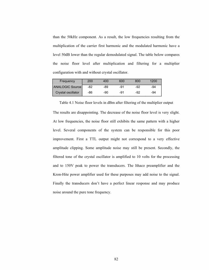
82

than the 50kHz component. As a result, the low frequencies resulting from the

multiplication of the carrier first harmonic and the modulated harmonic have a

level 50dB lower than the regular demodulated signal. The table below compares

the noise floor level after multiplication and filtering for a multiplier

configuration with and without crystal oscillator.

Frequency 200 400 600 800 1200

ANALOGIC Source -82 -89 -91 -92 -94

Crystal oscillator -86 -90 -91 -92 -94

Table 4.1 Noise floor levels in dBm after filtering of the multiplier output

The results are disappointing. The decrease of the noise floor level is very slight.

At low frequencies, the noise floor still exhibits the same pattern with a higher

level. Several components of the system can be responsible for this poor

improvement. First a TTL output might not correspond to a very effective

amplitude clipping. Some amplitude noise may still be present. Secondly, the

filtered tone of the crystal oscillator is amplified to 10 volts for the processing

and to 150V peak to power the transducers. The Ithaco preamplifier and the

Kron-Hite power amplifier used for these purposes may add noise to the signal.

Finally the transducers don’t have a perfect linear response and may produce

noise around the pure tone frequency.

83

Filtering of the output of the multiplier

Prior to acquisition on a computer, the output signal of the multiplier has

to be filtered to remove the high frequency component. Such a filtering is

necessary because aliasing would occur otherwise: the high frequency tone level

is so high that the dynamic range of a common A/D card would not allow

acquiring the low frequency component. Recall the expression of the output

signal of the multiplier device:

0.5*A1A2(cos(-k(d+δ (t)) + cos(2ωc t + k(d+δ (t))

The component at 2ωc rad/s needs to be filtered. An attenuation of 120dB

at 100kHz would decrease the level of this component to the level of a 1-

nanometer vibration. The signal could then be acquired by a low sampling rate

A/D card. Usually, filter manufacturers do not guaranty such high attenuations in

the stop band, so a filter was designed and implemented in the laboratory. In

order to get a flat amplitude response on the frequency range 100 to 800Hz, the

cutoff frequency has to be relatively high. Fc=10 kHz was chosen as a reasonable

value. Theoretically filters perform 6dB attenuation per octave and per pole. The

cutoff frequency and the 100kHz component are separated by a decade. Then, a 6

poles Chebyshev (with 1dB ripple) filter theoretically gives a 120 dB attenuation

at 100kHz [15]. Two filters built with three cascaded operational amplifiers

circuits were implemented on the same board along with two AD534 multipliers.

84

Figure 4.3 One stage of the Chebyshev active low pass filter

The resistors and capacitor were chosen to give a cutoff frequency of

10kHz.

Resistor (kΩ) Capacitor C1 (pF) Capacitor C2 (pF)

Stage 1 330 50 47

Stage 2 220 50 25

Stage 3 39 1500 100

Table 4.2 values of the resistors and capacitors for the filter

Low pass Chebychev active filter amplitude response

-100

-90

-80

-70

-60

-50

-40

-30

-20

-10

01 10 100 1000

Frequency in kHz

dB

Figure 4.4 Amplitude response of the active filter implemented on board

85

Measurements indicate that this filter performs a maximum attenuation of

90 dB in the stop band. Spectrum measurement of the filtered signal while the

system was running showed remaining 50kHz tones of a level of -60dBm.

Having the multipliers and the filters mounted on the same board is probably

responsible for this. A cross talk phenomenon can occur through the +/-15V

power line. However such a low level does not have much consequence. The

level of a nanometer vibration being -90dBm, the 50kHz tones are well in the

vertical range of the acquisition card. The advantage of the Chebyshev design is

that it provides a very sharp transition from the pass band to the stop band. On the

other hand, it has poor phase delay characteristics. The phase delay is not uniform

in the range 100Hz-800Hz and has to be corrected digitally. This can be

performed after acquisition of the signal.

86

Digital signal processing

After filtering of the output of the multiplier, several operations remain to

be computed to get the displacement of the ground. These operations can be

performed digitally, after acquisition on a computer. In particular additional

filtering of the high frequencies and the calculation presented in chapter III has to

be done. In order to sample a signal component at 100kHz, Niquist rule requires

that the signal should be acquired at a frequency over 200kHz. Also, the dynamic

range of the acquisition must be adequate for a resolution of the system of

1nanometer.

A VXI system performs acquisition of the signal, filtering and

calculations. It consists of a PC board and a waveform analyzer TVS 625 card.

The card acquires the two signals simultaneously at sampling frequency 250kHz.

The signals are coded on 8bits and the card can record up to 15000 samples in a

row on each channel. This allows a recording time of 6.10-2 second. During that

time a Raleigh wave would travel a distance of 4.8 meters.

The waveform analyzer card is controlled through a Labview interface.

The program developed performs an acquisition of the signals, filtering, and the

calculations required to compute the soil surface displacement. The filters

installed perform a 5 poles Bessel filtering with cutoff frequency of 5kHz.

Correction of the phase shifts originated by the analog filtering was not

implemented. The Labview code is attached.

87

Figure 4.5 LabView diagram of the digital signal processing

88

Conclusion

Dynamic range of the different devices of the system and signal to noise of the

signals could not be measured beyond 100dB. This limit, set by the measurement

capabilities of the spectrum analyzer, makes it difficult to locate the element

limiting the resolution of the whole system. Different sources of noise were

studied. Acoustic noise level at the frequency of the transducer was found to be

very low in the laboratory. These allow a dynamic range over 120dB when using

the transducer with a driving voltage of 150V peak and a distance of 55mm. In

order to limit electromagnetic cross talk, a shielded design was adopted for all the

components of the system. The source noise can be amplitude noise or phase

noise. The implementation of a delay line in the aim of improving the resolution

did not give measurable result. A crystal oscillator was introduced. It gave only a

slight reduction of the low frequency noise floor level. The remaining noise can

either be coming from the transducer or amplitude noise of the crystal oscillator.

For the filtering of the multiplier output, a sharp low pass filter is needed. An on-

board active Chebyshev design filter was implemented. It performs a 90dB

reduction at 100kHz. The remaining 100kHz tone was filtered after acquisition

on a computer.

89

CHAPTER VI

CONCLUSIONS

A system using 50kHz electrostatic transducers and analog demodulation

was implemented. It performs vibrations measurements adequate for use with

surface waves in the ground used for mine detection. A displacement sensitivity

on of 1-nanometer was obtained in the frequency range 400-1200Hz. In the low

frequency range, the resolution deteriorates down to a few nanometers at 200Hz.

The transducer system achieves a spot size of the order of a centimeter

compatible with surface wave measurement in the frequency range presented.

The choice of electrostatic transducers allowed high acoustic pressures,

over 120dB re 20µPa. Their very high receiving sensitivity permitted unamplified

signal levels over 500mV. These conditions were favorable to high signal to

noise ratio. The natural focusing of the transducers was used to get a small spot

size and higher signal levels. Spherical focusing of the sound was considered

between50kHz and 200kHz. A computer model based on the Raleigh integral

was developed to calculate the sound field of spherically focused transducers. In

particular, the results give focusing distances and pressure at the focused point for

transducers running at different frequencies. At 50kHz it seems difficult to focus

the sound more than a few centimeters away from the transducers. This will

certainly be impractical when used in the fields. However, the calculations

indicate that at 200kHz spherically focused transducers can focus at a distance of

13 centimeters with a pressure gain of four relative to the normalized pressure.

90

Such performances seem promising. Attenuation in the air should not be a

problem for distances less than a meter and frequencies up to 200kHz.

Capacitance transducers may not be ideal however due to the use of a high bias

voltage of 150 to 200 Volts. Such transducers may malfunction in difficult

environments. The bias voltage can easily be short-circuited accidentally. The

transducers may also age rapidly in highly corrosive environments.

With the aim of determining the equipment needed to perform a digital

demodulation of the signal, a study of data acquisition cards was done. A test on

a recent card showed a noise floor level too high to permit phase demodulation

with a sensitivity of 120dB. Computer models of the two noise sources for A/D

cards were developed. The corresponding noise floor levels were evaluated with

a resolution of one Hertz. Twelve and 16 bit coding allow resolutions of 115 and

140 dB respectively. The highest noise level on the card tests seemed to come

from the clock jitter. If the clock jitter level (in seconds) is inversely proportional

to the clock speed (or constant in degrees), a 1Gigahertz clock should be

adequate. Finally, specifications for an acquisition card for demodulating of a

50kHz carrier signal with a sensitivity of 120dB are acquisition on 2 channels,

16bit coding and a 1GigaHz clock. Due to the cost of such a device, efforts were

concentrated on an analog demodulation

Several analog demodulation configurations involving multiplication of

the signal with the carrier tone and low pass filtering were investigated. The

sensitivity of some multiplication devices was studied experimentally with the

transducer system. The transducer were aimed at a vibrating piston, mixers and

multipliers were used to demodulate the signal. Vibration from 200Hz to 1200 Hz

91

with amplitude of 40nanometer was used. A mixer setup was able to demodulate

the signal with a sensitivity of 100dB. Multiplier circuits gave higher output

levels with sensitivities up to 124dB. In all cases, a rise of the noise floor was

observed in the lower frequency range. Finally a complete demodulation

configuration was implemented with a quadrature circuit and on board filtering.

This quadrature of the carrier signal was obtained with an operational amplifier

differentiating circuit. It provides a gain of 1 at 50kHz and a phase shift of pi/2

with a dynamic range superior to 120dB.

Noise measurements were difficult to acomplish because of the high

sensitivity desired for the demodulation. Acoustic noise was not a problem thanks

to the very high source level of the transducer. Implementation of a delay line and

a crystal oscillator showed that the rise of the noise floor in the low frequency

range did not come from phase noise of the source. Transducer or source

amplitude noise are believed to be responsible for this phenomenon. A good

filtering of the multiplier output signal was obtained by implementation of on-

board active filtering.

92

CHAPTER VII

RECOMMENDATIONS FOR FURTHER STUDY

Some more research could continue on reducing the noise and improving

the sensitivity at low frequencies. The system will also have to be tested on

transient waves in the sand. Then, some more work could be conducted for more

practical outdoor use of the transducer system. In particular, this environment

would require more robust transducers able to function further from the ground.

Although the filtering installed is satisfactory, it could be optimized. In

particular, the active filtering of the multiplier output could be performed on a

board distinct from that of the multiplier chips, using a different power supply.

This configuration would reduce the cross talk of the 50kHz carrier tone and save

some digital filtering. The rise of the noise level in the low frequency range could

be further investigated. This rise reduces the resolution down to 112dB at 200Hz.

It is believed that the demodulation is not responsible for this phenomenon.

Therefore, Investigation should concentrate on the transducers and the source.

Noise from the crystal oscillator can only be amplitude noise and clipping of its

signal would reduce it. Using another type of transducer may provide a higher

quality signal. However, the noise problem will be very minor if a higher

frequency is chosen for the final system. To give an idea, a resolution of 114dB

would give a minimum sensitivity of 1-nanometer for frequencies over 100kHz.

93

A more important step would be to test the system in the experimental

sand tank. Some slight modification would have to be implemented for such

experiments. Analog and digital filtering of the multiplier output signals induce a

phase shift that is not uniform over frequency. This phase shifting has to be

determined and a digital correction must be implemented so that the system can

handle transient waves. This digital correction can be installed on the existing

Labview program.

At the same time, some research could be conducted for a more practical

“in situ” use of the system. The capacitance transducers are neither sealed, nor

robust. They run with a High DC bias of 150-200V. These weaknesses could

cause problems when using them in a humid or corrosive environment. Short

circuits are likely to happen at such a high voltages, possibly damaging the

system. Hence, long life of the batteries and the transducers is not guaranteed.

More robust transducers, such as most piezoelectric transducers, are

commercially available. They usually have a poorer receiving sensitivity, but

better focusing may be able to compensate for the corresponding loss in signal

level. Using the transducers in a typical outdoor environment would also require

a localization of the transducers at a larger distance from the soil. In order to keep

a small spot size, the sound beam will have to focus at this same distance. Some

theoretical work on the focusing of the sound has been accomplished, but

experimental tests remain to be conducted.

The most important issue for a practical use of this system could be the

presence of vegetation. Most of the land mines remaining to be removed have

been in the ground for a long time. Vegetation has had time to grow and hide the

94

soil surface. Herbs, plants and clutter could be at the same time, rigid enough for

ultrasound reflection, and isolated from the ground and the surface wave. This

issue would have to be investigated experimentally.

95

APPENDICES

96

% BIT NOISE SIMULATION: echo off;clear all; Fcarrier=49988; fs=250E3; Ts=1/fs;T=1; N=fs*T; Kc=2*50000*pi/340 t=(0:Ts:T-Ts); % 50kHz Pure tone with 200Hz phase modulation S=cos(2*pi*Fcarrier*(t)+2*Kc*1E-8*cos(2*pi*200*(t))); %16 bits model M=2^15; %+/-signal S1=round(M*S)/M; %12 bits model M=2^11; %+/-signal S2=round(M*S)/M; %Fourier Transform of the three signals freqs=(0:1:249999); figure(1); subplot(3,1,1); plot(freqs,20*log10(abs(fft(S)))); axis([49000,51000,-260,120]);grid on xlabel('frequency (Hz)'); ylabel('dB'); title('Fourier Transform of an Ideally Digitized Signal') subplot(3,1,2); plot(freqs,20*log10(abs(fft(S1)))); title('Fourier Transform of Ideally Sampled Signal with 16 Bits Coding') axis([49000,51000,-60,120]);grid on xlabel('frequency (Hz)'); ylabel('dB'); subplot(3,1,3); plot(freqs,20*log10(abs(fft(S2)))); title('Fourier Transform of Ideally Sampled Signal with 12 Bits Coding') axis([49000,51000,-60,120]);grid on xlabel('frequency (Hz)'); ylabel('dB');

97

% JITTER OF SAMPLING CLOCK SIMULATION: echo off;clear all; Fcarrier=50000; fs=250E3; Ts=1/fs;T=1; N=fs*T; Kc=2*50000*pi/340 t=(0:Ts:T-Ts); S=cos(2*pi*Fcarrier*(t)+2*Kc*1E-8*cos(2*pi*200*(t))); %clock jitter %5E-8s jitter amplitude err=.33333/20E6*randn(1,250000); t2=t+err; S1=cos(2*pi*Fcarrier*(t2)+2*Kc*1E-8*cos(2*pi*200*(t2))); %5E-9s Jitter amplitude err=.33333/20E7*randn(1,250000); t2=t+err; S2=cos(2*pi*Fcarrier*(t2)+2*Kc*1E-8*cos(2*pi*200*(t2))); %Graphs of the Fourier Transform freqs=(0:1:249999); figure(1); subplot(3,1,1); plot(freqs,20*log10(abs(fft(S)))); axis([49000,51000,-260,120]);grid on xlabel('frequency (Hz)'); ylabel('dB'); title('Fourier Transform of an Ideally Digitized Signal') subplot(3,1,2); plot(freqs,20*log10(abs(fft(S1)))); title('Fourier Transform of Sampled Signal with 5E-8s Jitter') axis([49000,51000,-60,120]);grid on xlabel('frequency (Hz)'); ylabel('dB') subplot(3,1,3); plot(freqs,20*log10(abs(fft(S2)))); title('Fourier Transform of Sampled Signal with 5E-9s Jitter') axis([49000,51000,-60,120]);grid on xlabel('frequency (Hz)'); ylabel('dB')

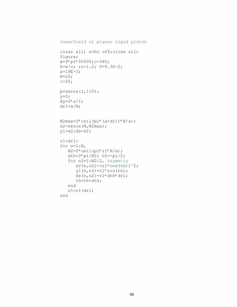
98

%nearfield of planar rigid piston clear all; echo off;close all; figure; w=2*pi*50000;c=340; k=w/c; ro=1.2; U=9.3E-2; a=19E-3; N=20; I=20; p=zeros(I,110); y=0; dy=2*a/I; dr1=a/N; N2max=2*ceil(pi*(a+dr1)*N/a); x2=zeros(N,N2max); y1=x2;ds=x2; r1=dr1; for n=1:N, N2=2*ceil(pi*r1*N/a); dth=2*pi/N2; th=-pi/2; for n2=1:N2/2, %symetry x2(n,n2)=(r1*cos(th))^2; y1(n,n2)=r1*sin(th); ds(n,n2)=r1*dth*dr1; th=th+dth; end r1=r1+dr1; end

99

z=1E-3; dz=.002; for l=1:110, zscale(l)=z; y=0; for i=1:I, yscale(i)=y; r=sqrt(x2+(y-y1).^2+z^2); ptemp=exp(-j*k*r)./r.*ds; p(i,l)=sum(sum(ptemp)); y=y+dy; end l z=z+dz; end p=2*j*p*ro*c*U*k/(2*pi); p1=abs(p); pdB=20*log10(p1/20E-6); contour(zscale,yscale,pdB,30); colorbar; xlabel('Distance on Transducer Axis (meter)','Fontsize',14) ylabel('Radial Axis','Fontsize',14)

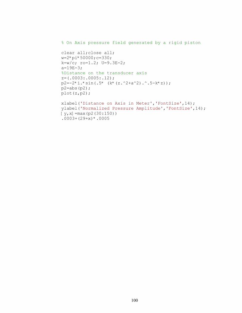
100

% On Axis pressure field generated by a rigid piston clear all;close all; w=2*pi*50000;c=330; k=w/c; ro=1.2; U=9.3E-2; a=19E-3; %Distance on the transducer axis z=(.0003:.0005:.12); p2=-2*i.*sin(.5* (k*(z.^2+a^2).^.5-k*z)); p2=abs(p2); plot(z,p2); xlabel('Distance on Axis in Meter','FontSize',14); ylabel('Normalized Pressure Amplitude','FontSize',14); [y,x]=max(p2(30:150)) .0003+(29+x)*.0005

101

% nearfield of spherically focused transducer clear all; echo off;close all; figure; w=2*pi*200000;c=340; k=w/c; ro=1.2; U=9.3E-2; %Radius of the transducer a=19E-3; %Geometrical focal distance Rf=.05; N=40; I=35; %Pressure on Plane limited by transducer axis p=zeros(I,70); y=0;z=5E-3; %ordinate increment dy=2*a/I; dgam=a/(Rf*(N+1)); gam=dgam/2; N2max=2*round(pi*Rf*sin(gam+N*dgam)/dgam); x1=zeros(N,N2max); y1=x1;z1=x1;ds=x1; %discretisation of the transducer surface coordinate (x1,y1,z1) area of surface element dS for n=1:N, N2=2*ceil(pi*Rf*sin(gam)*N/a); dth=2*pi/N2; th=-pi/2+dth/2; dst=Rf^2*sin(gam)*pi*2/N2*dgam; %gap1(n)=Rf*sin(gam)*cos(th); for n2=1:N2/2, %symetry x1(n,n2)=Rf*sin(gam)*cos(th); y1(n,n2)=Rf*sin(gam)*sin(th); z1(n,n2)=-sqrt(Rf^2-x1(n,n2)^2-y1(n,n2).^2)+Rf; ds(n,n2)=dst; th=th+dth; end %gap2(n)=Rf*sin(gam)*cos(th); gam=gam+dgam; end % calculation of the pressure field with the Raleigh integral

102

dz=.001; z=0.001; for l=1:70, zscale(l)=z; y=0; for i=1:I, yscale(i)=y; if z>(Rf-sqrt(Rf^2-y^2)) r=sqrt(x1.^2+(y-y1).^2+(z-z1).^2); ptemp=exp(-j*k*r)./r.*ds; p(i,l)=sum(sum(ptemp)); elseif z>.008 r=sqrt(x1.^2+(y-y1).^2+(z-z1).^2); ptemp=exp(-j*k*r)./r.*ds; p(i,l)=sum(sum(ptemp)); end y=y+dy; end z=z+dz; end p=2*j*p*ro*c*U*k/(2*pi); p1=abs(p); pdB=20*log10(p1/20E-6); contour(zscale,yscale,pdB,30); xlabel('distance on symmetry axis in meters','FontSize',12); ylabel('Radial Distance','FontSize',12); colorbar; figure; pnorm=p1(1,:)/(ro*U*c); plot(zscale,pnorm); xlabel('Distance on Symmetry Axis in Meter','FontSize',12); ylabel('Radial Distance','FontSize',12);

103

REFERENCES

[1] Kosta Tsipis,”Technological innovation in humanitarian demining” , Proceedings of the Human Factors and Ergonomics Society vol.1 1998, p750-753 [2] N. Goldfine, D. Clark “ New quasistatic magnetic and electric field imaging arrays and algorithms for object detection identification and discrimination”, Proceedings of the 1999 Detection and remediation Technologies for Mines and Minelike Targets IV.

[3] Smith, Preston S. Wilson, Fred W. Bacon, et al., “Measurement and Localisation of Interface Wave Reflections from a Buried Target”, University of Texas at Austin, August 1997. [4] Don, C.G. and D.E. Lawrence, “Detecting Buried Objects, Such as Land Mines, Using Acoustic Impulses” Echoes, Winter 1998. [5] W. R. Scott, Jr., and J.S. Martin, “An acousto-electromagnetic sensor for locating land mines” in Detection and Remediation Technologies for Mines and MinelikeTargets III, Proc. SPIE 3392, pp 176-186, 1998. [6] W. R. Scott, Jr., and J.S. Martin, “Experimental investigation of the acousto-electromagnetic sensor for locating land mines” in Detection and Remediation Technologies for Mines and MinelikeTargets IV, Proc. SPIE, 1999. [7] W. R. Scott, C. Schroeder, J.S. Martin, G. Larson “Investigation of a technique that uses both elastic and electromagnetic waves to detect buried land mines” in proceedings of AP2000 -Millennium conference on Antennas and propagation, Davos, Switzerland, April 2000. [8] W. R. Scott, J.S. Martin, G. Larson “Experimental Model for a Seismic Landmine Detection System” IEEE Transactions on Geoscience and Remote Sensing 2000 [9] C. T. Schroeder W. R. Scott, Jr., “Finite difference time domain model for elastic waves in the ground” Proceedings of SPIE Vol 3710, April 1999. [10] P.H. Rogers, M. Cox, “Automated noninvasive Motion Measurement of Auditory Organs in Fish Using Ultrasound” from Journal of Vibration, Acoustics, Stress, and Reliability in Design January 1987. [11] Kouwenhoven and Michael Hendrikus Laurentius, “High-performance frequency-demodulation systems” published by Delft University Press, 1998.

104

[12] Technical data “Ultrasonic Ranging System” Polaroid 1984 [13] C.Bilber, S. Ellin, E. Shenk, and J. Stempeck “The Polaroid Ultrasonic Ranging System” 1980 [14] Joe Adler “Jitter in Clock sources”,Vectron International http://www.vectron.com/whatsnew/jitter.htm [15] Arthur B. Willams, Fred J. Taylor “Electronic Filter Design Handbook” third edition 1995.