detection of subsurface voids in stratified media …
TRANSCRIPT

The Pennsylvania State University
The Graduate School
Department of Civil and Environmental Engineering
DETECTION OF SUBSURFACE VOIDS IN STRATIFIED MEDIA USING
SEISMIC WAVE METHODS
A Thesis in
Civil Engineering
by
Ashutosh Srivastava
2009 Ashutosh Srivastava
Submitted in Partial Fulfillment
of the Requirements
for the Degree of
Master of Science
May 2009

The thesis of Ashutosh Srivastava was reviewed and approved* by the following:
Jeffrey Laman
Associate Professor of Civil and Environmental Engineering
The Pennsylvania State University
Thesis Advisor
Andrea J. Schokker
Professor and Head of Civil Engineering, University of Minnesota Duluth
Angelica Palomino
Assistant Professor of Civil and Environmental Engineering
The Pennsylvania State University
Peggy A. Johnson
Head of the Department of Civil and Environmental Engineering
The Pennsylvania State University
*Signatures are on file in the Graduate School

ii
ABSTRACT
The primary objective of this study is to investigate the effect of sub-surface
anomalies such as voids in the stratified soil media on surface wave propagation. A data
processing protocol was developed for processing seismic wave data for void detection
by studying the signal simultaneously in the time and frequency domain using continuous
wavelet transformation (CWT). The effect of voids in the soil media was examined by
qualitatively comparing the signal properties acquired from the controlled laboratory
experiments on the soil media, both with and without voids. For the controlled
experimental study, a wooden box of dimensions 4.5m x 1.67m x 1.37m ( 64x65x51 ′′′′′′′ ),
was constructed and filled with sand and gravel in two layers. A void of known
dimension was excavated in the soil mass in the box at a known location. Micro seismic
waves were produced using a 7.25kg (16-lb) sledge hammer and a rubber mallet. The
vertical response of the soil mass surface was recorded using the SignalCalc®620
Dynamic Signal Analyzer and was processed using the MATLAB® 7.0 wavelet toolbox.
Time-frequency plots of the seismic wave signals obtained from the unvoided soil mass
experiment indicate that damped, uniform undulations are due to the surface wave
dispersive behavior. Also, data obtained from the voided soil mass experiment indicate
that the void anomalies cause low strength ripples in the time-frequency plots, usually in
the low frequency region of the time-frequency plots. This observation has been used to
study the properties of voids.
In addition to the experimental study, a numerical study was also conducted. The
wave propagation phenomenon was simulated for voided and stratified regions using the
iii
finite difference method in the Wave2000pro software. Thus, a refraction test was
performed in the soil box to determine the shear wave velocity profile. The receiver data
was processed with the same protocol that was used for analyzing the experimental test
data conducted in the soil box with void. The time-frequency maps constructed using the
experimental data confirm the numerical results.
Finally, the time-frequency maps using different types of wavelets for the same
set of experimental data were compared. From this analysis it was concluded that the
wavelets that correlates with the properties of the original signal produce time-frequency
plots with all the signal features distinctively so that all the signal properties can be
separately studied. Thus, wavelet analysis of the seismic wave signals obtain from the
micro-seismic tests can effectively investigate the sub surface void anomalies.

iv
TABLE OF CONTENTS
LIST OF FIGURES .......................................................................................................... ix
LIST OF TABLES............................................................................................................ xii
ACKNOWLEDGEMENTS............................................................................................. xiii
CHAPTER 1 INTRODUCTION ...................................................................................... 1
1.1 Background ................................................................................................................... 1
1.2 Problem Statement ........................................................................................................ 4
1.3 Objectives ..................................................................................................................... 5
1.4 Scope of Research ......................................................................................................... 5
1.5 Organization of Report ................................................................................................. 6
CHAPTER 2 LITERATURE REVIEW ......................................................................... 7
2.1 Introduction ................................................................................................................... 7
2.2 Elastic Wave Propagation in Homogenous, Isotropic Half-space ................................ 7
2.3 Seismic Wave Methods .............................................................................................. 10
2.3.1 Seismic Refraction Survey .............................................................................. 11
2.3.2 Seismic Reflection Survey................................................................................ 13

v
2.3.3 Surface Wave Methods..................................................................................... 15
2.4 Applicability of Seismic Methods in Void and Sinhole Detection ............................ 16
2.5 Analysis of Seismic Test Data ................................................................................... 19
2.5.1 Time-history Analysis ...................................................................................... 19
2.5.2 Wavelet Analysis ............................................................................................. 22
2.5.2.1 Continous Wavelet Transformation (CWT) ........................................ 22
2.5.2.2 Wavelet Families .................................................................................. 31
2.5.2.2.1 Daubechies Wavelets ............................................................ 32
2.5.2.2.2 Symlet Wavelet Family ........................................................ 33
2.5.2.2.3 Meyer Wavelet ..................................................................... 33
2.4.2.2.4 Mexican Hat Wavelet ............................................................ 34
2.4.2.2.5 Gaussian Wavelet Family ..................................................... 35
2.6 Numerical Simulation of Wave-propagation in Elastic Media .................................. 36
2.7 Summary..................................................................................................................... 40

vi
CHAPTER 3 TESTING PROGRAM ........................................................................... 41
3.1 Introduction................................................................................................................. 41
3.2 Data Acquisition System ............................................................................................ 41
3.2.1 Signal Analyzer ................................................................................................ 42
3.2.2 Geophones ....................................................................................................... 43
3.2.3 Energy Source................................................................................................... 44
3.2.4 Data Acquisition Software................................................................................ 45
3.3 Laboratory Test Setup................................................................................................. 46
3.4 In-situ Soil Properties Tests: Refraction Test on Soil Box ......................................... 50
3.5 Summary..................................................................................................................... 52
CHAPTER 4 NUMERICAL SIMULATION............................................................... 53
4.1 Introduction................................................................................................................. 53
4.2 Parameters for FDTD Simulation of Wave Propagation Phenomenon ..................... 53
4.2.1 Image Size ........................................................................................................ 54
4.2.2 Material Properties............................................................................................ 54
4.2.3 Boundary Condition.......................................................................................... 55

vii
4.2.4 Source Confiurgation........................................................................................ 55
4.2.5 Receiver Confiugration..................................................................................... 56
4.2.6 Time Step Scale ................................................................................................ 56
4.2.7 Maximum Frequency........................................................................................ 56
4.3 Numerical Simulation of Wave Propagation in Layered Media................................. 57
4.4 Summary..................................................................................................................... 59
CHAPTER 5 RESULTS AND DISCUSSION.............................................................. 60
5.1 Introduction................................................................................................................. 60
5.2 Data Processing........................................................................................................... 60
5.2.1 Data Processing Software ................................................................................. 61
5.2.1.1 MATLAB® 7.0 Programming Platform and Wavelet Toolbox............ 61
5.2.1.2 Seisimager®2D...................................................................................... 61
5.2.2 Data Processing Protocol .................................................................................. 62
5.3 Data Processing Results.............................................................................................. 64
5.3.1 In-situ Refraction Survey for In-site Shear Wave Velocity Profile.................. 64
5.3.2 Wavelet Analysis of the Experimental Data..................................................... 65
viii
5.3.2.1 Analysis Using Different Wavelet Families ......................................... 65
5.3.2.2 Wavelet Analysis of Soil Box Test Data .............................................. 68
5.3.3 Wavelet Analysis of the Numerical Simulation Data....................................... 75
5.4 Summary..................................................................................................................... 78
CHAPTER 6 SUMMARY AND CONCLUSIONS...................................................... 80
6.1 Summary..................................................................................................................... 80
6.2 Conclusions................................................................................................................. 81
6.3 Recommendations for Future Research ...................................................................... 83
REFERENCES................................................................................................................ 84
APPENDIX A .................................................................................................................. 88
APPENDIX B .................................................................................................................. 89

ix
LIST OF FIGURES
Figure 2.1. P, S and R-waves in Elastic Isotropic Homogenous Half-space ...................... 9
Figure 2.2. Seismic Refraction Geometry......................................................................... 13
Figure 2.3. Seismic Reflection Geometry......................................................................... 15
Figure 2.4. Travel-time Curve .......................................................................................... 20
Figure 2.5. Arrival Time Estimation of Reflected Waves from Horizontal
Interface................................................................................................................. 20
Figure 2.6. Sine Function with Different Scales............................................................... 23
Figure 2.7. db2 Wavelet Function with Different Scales.................................................. 24
Figure 2.8. Place the Scaled Wavelet at the Signal Origin and Calculate Wavelet
Coefficient ................................................................................................................. 26
Figure 2.9. Shift the Scaled Wavelet to New Time Location and Calculated
Wavelet Coefficient .................................................................................................. 26
Figure 2.10(a). Three Dimensional Wavelet Coefficient Plot .......................................... 27
Figure 2.10(b). Contour Plot of Wavelet Coefficients...................................................... 27
Figure 2.11. Synthetic Signal............................................................................................ 28
Figure 2.12. Power Spectral Density Plot of the Signal given by Equation 2.4 ............... 29
x
Figure 2.13. Wavelet Coefficient Map ............................................................................. 30
Figure 2.14. Daubechies Wavelet Family......................................................................... 33
Figure 2.15. Symlet Wavelet Family ................................................................................ 33
Figure 2.16. Meyer Wavelet ............................................................................................. 34
Figure 2.17. Mexican Hat Wavelet ................................................................................... 34
Figure 2.18. Gaussian Wavelet of Order 1 ....................................................................... 35
Figure 2.19. Surface Wave Front ...................................................................................... 36
Figure 2.20. Sample Grid and Cells.................................................................................. 39
Figure 3.1 General Layout of the Data Acquisition System Setup................................... 42
Figure 3.2. Gisco SN4 Geophones.................................................................................... 43
Figure 3.3 (a). Wooden Test Box Layout ......................................................................... 46
Figure 3.3 (b). Wooden Test Box .................................................................................... 47
Figure 3.4(a). Test Setup Scheme Without Void.............................................................. 49
Figure 3.4 (b). Test Setup Scheme for Void Detection..................................................... 50
Figure 3.4 (c). Void Detail (Section 1-1).......................................................................... 50
Figure 3.5 (a). Test Setup for Refraction Test #1 ............................................................. 51

xi
Figure 3.5 (b). Test Setup for Refraction test #2 .............................................................. 52
Figure 4.1. Numerical Model Setup.................................................................................. 57
Figure 5.1. Protocol for Data Processing .......................................................................... 62
Figure 5.2 (a) Shear Wave Velocity Profile for Refraction Test #1 Conducted on
Full Length Soil Box............................................................................................ 64
Figure 5.2 (b) Shear Wave Velocity Profile for Refraction Test #2 Conducted on
Full Length Soil Box............................................................................................ 65
Figure 5.3. Figure 5.3. Time-Frequency Plot for Channel 6 Generated from
7.25kg (16 lb) Sledgehammer on Soil Box with Void Using Different
Types of Wavelet ................................................................................................. 67
Figure 5.4. Time-Frequency Plot for Channels 1, 4, and 10 Generated from
7.25kg (16 lb) Sledgehammer on Soil Box without Void..................................... 70
Figure 5.5. Time-frequency Plot for Channels 1, 4, and 10 Generated from 7.25kg
(16 lb) Sledgehammer on Soil Box with Void..................................................... 72
Figure 5.6. Time-frequency Plot for Channels 1, 4, and 10 Generated from Rubber
Mallet on Soil Box with Void .............................................................................. 74
Figure 5.7. Time-frequency Plot of Receivers 1, 4, and 10 Generated from
Numerical Simulation .......................................................................................... 76

xii
LIST OF TABLES
Table 2.1. Wavelet Families ............................................................................................. 32
Table 3.1. Portable Computer Specifications ................................................................... 44

xiii
ACKNOWLEDGEMENTS
I would like to thank my committee members Dr. Jeffrey Laman, Dr Andrea
Schokker and Dr Angelica Palomino, with special thanks to Dr. Laman and Dr. Schokker
for their advising roles. I would also like to thank Edwin Rueda who assisted with the
construction of the wooden soil box and testing. This study was supported by the
Pennsylvania Transportation Institute and the Pennsylvania Department of
Transportation. I am thankful for their financial support. Finally, my sincere thanks go to
my fiancée, Janani Iyer and my family. Without there motivation, support, love and
encouragement, this accomplishment would not have been possible.
1
Chapter 1
Introduction
1.1 Background
Detection of obstacles, voids, cavities, subsurface rock profiles, or underground
utilities is required for the planning, design, and remediation of existing sub-structures
(foundations, tunnels or basements). These sub-surface features affect the soil properties
such as shear strength, shear modulus, in-situ density and bed rock profile in their
vicinity. The design and planning process of any sub-structure are primarily dependent on
these sub-surface soil properties. Detection of these sub surface features has received
much consideration due to rapid formation of sinkholes and damage to infrastructure
(Alexander and Book 1984; Canace and Dalton 1984; Stewart 1987). Most of the
currently used, traditional methods of determining the soil properties are laboratory based
tests and require transportation of the soil samples from the site. The collection and
transportation of soil samples results in a disturbed sample and thus may not represent the
soil conditions in-situ (Powrie 2004). The other drawback of laboratory testing is that the
procedure requires a fixed time for transporting samples and conducting tests. To
overcome the drawbacks of the laboratory testing, a large variety of in-situ tests were
developed. These tests include the vane shear test, cone penetration method, sand cone
replacement method, bore-hole shear test, rock pressure meter test, dilatometer test,
KoStep blade test, and rock shear test (Roy 2007). These in-situ tests are very quick and
can provide results in real time. However, they may require sophisticated instruments and

2
substantial manpower. Another drawback of in-situ tests is that the depth of exploration
of these tests is limited to near the surface, and the spatial resolution of the variation of
the soil properties is poor. To overcome the resolution problem, non-destructive, in-situ
tests were developed. These methods include multi-channel analysis of surface waves
(MASW), spectral analysis of surface waves (SASW), seismic refraction survey, seismic
reflection survey, electrical imaging, ground penetrating radar, subsurface penetrating
radar, and microgravity survey (Belesky and Hardy, 1986). Most of these exploration
methods are based on the generation-collection methods. In these methods radio or
acoustic waves, or electric current is generated in the ground and the surface vertical
response or electric current is measured with the help of geophones or electrodes. Then,
the data is processed and deductions are made about the sub-surface soil properties based
on the data analysis. These methods vary widely in feasibility, cost to benefit ratio,
applicability, and effectiveness.
Dobecki and Upchurch (2006) compared the effectiveness of various geophysical
methods in detecting sinkholes and other ground subsidence and concluded that seismic
wave based sub-surface exploration techniques are very successful in determining the
elastic moduli of the soil layers surrounding these ground features. Seismic wave based
exploration techniques utilize different types of data processing tools to extract the
medium property information about the medium. Seismic methods include the travel time
estimation or spectral analysis of the elastic waves (surface waves, compression waves
and shear waves) generated in a medium due to an impact on the ground surface (Richart,
Woods, and Hall 1970). Travel time based methods include the refraction and reflection

3
method and spectral analysis methods include spectral analysis of surface waves (SASW)
and multichannel analysis of surface waves (MASW).
Most of the current commercially available software for the seismic wave data
processing, such as Seisimager®
2D and Surfseis®
, identify the surface wave component
with a built-in algorithm and estimate the quality of the signal based on the power and
arrival time of the surface wave component. In some cases, the software algorithm for
surface wave identification fails due to ripples in the signal generated from the reflection
of waves from voids and other anomalies (Park, and Heljeson 2006). Thus, there is a need
for an efficient and accurate procedure for the surface wave identification during signal
processing.
Signal processing techniques have improved exponentially due to advancements in
the available computational resources. Signals can now be analyzed more effectively and
quickly using different methods simultaneously (Yilmaz 1987; Tokimatsu 1997; Ganji,
Gucunski, Nazarian 1998). These methods include Fourier analysis, time domain
analysis, time-series analysis, wavelet analysis and fractal analysis. Recently, wavelet
transformation has gained popularity due to its wide range of applicability (Shokouhi and
Gucunski 2003). Traditional spectrum analysis only provides the frequency content of the
signal but contains no information on the location of the signal where these frequencies
are occurring. However, wavelet transforms can be used to study the time localization of
the signal (the variation of the frequency content of the signal with time) (Walker 1999).
Kaiser (1994) defined the wavelet transformation as, “…the convolution between a
function known as wavelet and the original signal.” The convolution result is used to
4
form time-frequency maps to give a representation of the signal in both the time and
frequency domain.
1.2 Problem Statement
The conventional seismic wave test approach that are generally used to estimate the
soil properties at the site of interest lacks the information of spectrum variation in the
time domain due to the presence of cavities and layers of soil. The spectrum variation
information of the reflected waves from any cavities or anomalies is lost when a Fourier
transform is performed on seismic test data. Travel time based methods that are generally
used in the case of reflection and refraction of seismic waves do not supply information
about change in frequency content. Time-frequency maps can be used to study the change
in frequency content over time and thus can be used for cavity detection in the region
with distributed soil properties.
This research demonstrates a new scheme for the detection of voids by analyzing the
surface wave component of a signal travelling through voided stratified soil media by
improving on the currently available signal processing methods used in the seismic wave
tomography. The focus is on the analysis of data obtained from the seismic wave tests
using different families of wavelets and development of a scheme for detecting voids in
the soil media. In this study the wave propagation was considered as elastic because these
seismic tests the strains produced by the impact are small and the media particles are not
permanently deformed.

5
1.3 Objectives
The primary objectives of this research are as follows:
• Develop a method to identify the surface wave component from the signal
generated by the seismic wave test using wavelet transform in the voided soil
media.
• Propose the most efficient and effective mother wavelet for seismic wave test
applications by investigating the effect of different types of wavelets on the
analysis.
• Develop a wavelet based protocol for processing of seismic wave data for
void detection.
1.4 Scope of Research
This research focuses on the development of a protocol for processing seismic wave
data for void detection using wavelet transformation. Other methods of void detection,
uncertainties associated with the measurement of data, participation of higher Raleigh
wave modes, data scatter and systematic error (Marosi 2004; Tuomi 1999) are not
examined in this study. Also the effect of porosity and saturation level of the soil was not
considered. The primary method used to investigate wave propagation in stratified voided
media consists of micro-seismic tests conducted under laboratory conditions. The data is
analyzed using wavelets from different classes, or families, to investigate the effect of
wavelet selection on wavelet analysis and the generation of time-frequency plots. The
effect of voids is studied simultaneously in the time domain as well as the frequency
domain using time-frequency plots generated from wavelet analysis of the signals. A
numerical model is developed using finite difference methods and focuses on simulation
6
of wave propagation in stratified voided soil media. The numerical model is then used to
study the wave propagation in the voided soil media. Results from the numerical
simulation and the laboratory tests are utilized to develop a protocol for the void
detection in the stratified soil media.
1.5 Organization of Report
Chapter two presents a literature review of the relevant studies on the fundamentals of
wave propagation phenomenon in elastic media and seismic wave test methods. The
wavelet transformation is also briefly discussed. The finite difference simulation of wave
propagation phenomenon in stratified soil media is reviewed.
Chapter three presents details of the testing program. It includes a description of the
data acquisition system and laboratory test setups. Chapter three also reviews soil
property tests conducted to provide input data for the finite difference simulation model.
Chapter four investigates the aspects of numerical modeling of wave propagation in
stratified soil media and an overview of the parameters associated with finite difference
time domain (FDTD) simulation of wave propagation in elastic media, and also the
numerical model used for the simulation of the soil box test.
Chapter five presents details of the analytical program related to laboratory testing
and an overview of the data processing methods used for analyzing laboratory tests and
numerical simulation test data. Also included are the results from all laboratory tests.
Chapter five also presents a detailed discussion of numerical simulation results and
comparison with experimental results. Chapter six provides a summary and conclusions
from the research and recommendations for future research.

7
Chapter 2
Literature Review
2.1 Introduction
There has been a large volume of research completed on the development of seismic
wave based sub-surface exploration techniques such as the seismic refraction survey and
seismic reflection survey. These techniques typically use time or frequency domain based
data analysis methods. But seismic wave test data is localized in time and, therefore, the
current time and frequency domain methods are not sufficient to extract all the
information from the data. Time-frequency maps are a representation of the signal in both
time and frequency domain and thus more information can be extracted from the signal
by studying it in both domains, rather than in a single domain. Very limited research has
been conducted relative to time-frequency domain analysis, particularly with regard to
wavelet transformation. This literature review highlights some of the pertinent research
regarding traditional seismic wave sub-surface exploration test data analysis procedures,
the applicability of these traditional seismic wave methods in void detection, and an
introduction to the wavelet transformation. Also included is an overview of wave
propagation phenomenon in elastic media and a discussion of the different types of
waves. Finally, the fundamentals of finite difference and its capability to accurately
model wave propagation phenomenon is discussed.
2.2 Elastic Wave Propagation in Homogeneous, Isotropic Half Space
In a three dimensional homogenous and isotropic medium, the equations of motion
for an elastic wave are written as (Richart, Woods, and Hall 1970):

8
i
2
i
2
i
2
uGx
)G(t
u∇+
∂ε∂
+λ=∂
∂ρ (2.1)
where,
ρ = density of the elastic medium.
ui = (u, v, w)T, is the displacement vector in the cartesian co-ordinates.
xi = (x, y ,z )T, ε is the cubical dilation and is equal to the volume strain of the
system.
λ = Lame’s first constant
G = Lame’s second constant or shear modulus.
∇ = Laplacian operator in the cartesian co-ordinates.
For a homogenous and isotropic elastic half-space, Equation (2.1) results in three
solutions, representing three types of waves: (1) dilatational wave, (2) distortional wave,
and (3) surface wave:
1. Dilatational wave (Primary wave, P-wave, pressure waves, compression
waves):
P-waves result in the dilatation of the medium. In the region affected by P-
waves, the medium particles vibrate along, or parallel to, the direction of
travel of the wave energy. The P-wave velocity is highest among all the wave
types discussed here (P, S and R). P-waves carry only 7 percent
(approximately) of the total energy (Richart, Woods, and Hall 1970).
2. Distortional wave (Secondary wave, S-wave, shear waves):
S-waves result in the distortion of the medium. In the region affected by S-
waves, the medium particles vibrate perpendicular to the direction of wave

9
propagation. The wave velocity of S-waves is greater than R-waves but less
than P-waves. Approximately 26 percent of the total energy is carried by S-
waves (Richart, Woods, and Hall 1970).
3. Surface wave (Rayleigh wave, R-wave):
R-waves move across the free surface and are confined to a zone near the free
boundary of the half-space. As it passes, a surface particle moves in a circle or
ellipse in the direction of propagation, depending on the medium properties.
The amplitude of the R-waves decreases rapidly with depth. R-waves decay
slowly with distance in comparison to the body waves (P- and S-waves), and
their velocity is slightly less than that of S-waves. Surface waves carry
approximately 67 percent of the total energy (Richart, Woods, and Hall 1970).
Figure 2.1. P-, S- and R-waves in Elastic Isotropic Homogenous Half-space
(Richart, Woods, and Hall 1970)
Source

10
The above discussion includes wave propagation in a homogeneous and
continuous elastic media. However, soil media is porous. Biot M.A, (1956) studied the
propagation of elastic waves in a fluid-saturated porous solid and concluded that wave
propagation in a fluid saturated porous solid media results in two dilation waves. He
termed them: “wave of the first kind” and “wave of the second kind”. He also concluded
that the wave velocity of the first kind wave was higher than the second kind wave.
However, wave of second kind showed the higher attenuation than the wave of first kind.
Berryman J.G., (1982) further investigated the effect of porosity on the wave velocity of
the two dilation waves and the shear wave and concluded that the velocity of the wave of
first kind decreases as the porosity of the media is increased. However, the velocity of the
wave of second kind increases as the porosity increases and also the shear wave velocity
also decrease as the porosity increases.
In this research, the effect of porosity and the saturation level were not
considered. The soil media was assumed to be a homogeneous solid media and elastic
wave propagation was considered.
2.3 Seismic Wave Methods
Conventional laboratory or on site methods of determining soil properties are: (1)
triaxial shear test, (2) vane shear test, (3) direct shear test, (4) uniaxial shear test, and (5)
cone penetration method. These are either performed on the samples from the site or on
the site. However, with these methods it is difficult to determine in-situ soil properties
below the uppermost layers. Richart, Woods, and Hall (1970) and Dobecki and Upchurch
(2006) investigated seismic wave methods and concluded that seismic wave methods are
advantageous in determining in-situ soil properties efficiently as they are performed on

11
the surface. With the use of wave propagation physics principles, important soil
properties can be determined at lower depths. There are generally three types of seismic
surveys conducted for subsurface soil profiling: (1) seismic refraction survey, (2) seismic
reflection survey, and (3) seismic surface wave methods.
2.3.1 Seismic Refraction Survey
Seismic refraction surveys are a commonly used, traditional, geophysical technique to
determine soil properties, depth of bedrock, water table depth, or other density contrasts
(Dobecki, and Romig 1985). The seismic refraction method has been used extensively to
characterize sub-surface soil conditions at environmental and engineering sites.
Redpath (1973) formulated a seismic refraction survey procedure for data acquisition
and processing. He summarized the theory and practice of using a refraction survey for
shallow and sub-surface investigations. A seismic refraction survey requires
measurement of travel time of the seismic energy component generated by a seismic
source selected on the basis of seismic line length resolution desired, and environmental
suitability of the seismic source. The P-wave or S-wave travels down to the top of rock
(or other distinct density contrast), is refracted along the top of rock, and returns to the
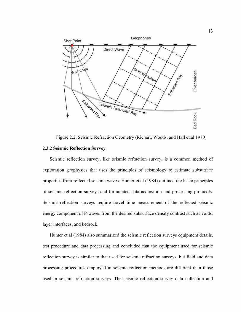
surface as a head wave along a wave front (Figure 2.2) (Richart, Woods, and Hall 1970).
Based on the typical energy sources used during a refraction test, the refraction survey is
limited to the mapping of soil layers that occur at depths less than 30.5m ( 010 ′ ). If a
seismic refraction survey is required for greater depths, then the geophone array spacing
is increased. However, due to site dimensions and input energy restrictions, achieving
results for depths more than 30.5m ( 010 ′ ) is practically not feasible. The major
disadvantage of seismic refraction occurs where a soil layer of low wave velocity

12
underlies a soil layer of high wave velocity. In these circumstances, seismic refraction
fails to detect the underlying low velocity layer.
Seismic refraction survey data processing is based on a first arrival concept (Redpath,
1973). Data processing requires manual selection of the P-wave arrival times from the
signal at each geophone location. During the selection process, knowledge of the seismic
wave propagation is required to differentiate the refracted P-wave arrival time from other
seismic waves, such as surface waves and S-waves. Thus, identification of each wave
class is required within the signal for accurate arrival time determination. The traditional
method assumes that the P-wave arrival coincides with the seismic wave energy arrival,
i.e. the arrival time of P-waves at a geophone is the time at which the data acquisition
system records the first non-zero reading at the geophone. This assumption is based on
the fact that P-waves travel faster than other seismic waves, such as surface waves and S-
waves. But, in a region with extreme tomography, this assumption may fail and leads to
erroneous results due to reflections from the void anamolies. Advanced inversion
methods are available in some commercial software such as Seisimager2D®
that utilize a
complex ray tracing algorithm to image relatively small targets such as foundation
elements. Software, such as Seisimager2D®
, can be utilized to perform refraction
profiling in the presence of localized low velocity zones such as voids (Geometrics, Inc.
2006). However some software may require accurate picking of P-wave arrival time.
13
Figure 2.2. Seismic Refraction Geometry (Richart, Woods, and Hall et.al 1970)
2.3.2 Seismic Reflection Survey
Seismic reflection survey, like seismic refraction survey, is a common method of
exploration geophysics that uses the principles of seismology to estimate subsurface
properties from reflected seismic waves. Hunter et.al (1984) outlined the basic principles
of seismic reflection surveys and formulated data acquisition and processing protocols.
Seismic reflection surveys require travel time measurement of the reflected seismic
energy component of P-waves from the desired subsurface density contrast such as voids,
layer interfaces, and bedrock.
Hunter et.al (1984) also summarized the seismic reflection surveys equipment details,
test procedure and data processing and concluded that the equipment used for seismic
reflection survey is similar to that used for seismic refraction surveys, but field and data
processing procedures employed in seismic reflection methods are different than those
used in seismic refraction surveys. The seismic reflection survey data collection and

14
processing procedures are intended to maximize the energy reflected along vertical ray
paths by subsurface density contrast (Figure 2.3) (Steeples and Miller, 1990). In a seismic
reflection survey, the first arrival data at the geophones do not represent reflected seismic
energy. The reflected component of seismic energy is identified by collecting and
filtering multi-fold or highly redundant data from numerous shot points per geophone
placement in a complex set of overlapping seismic arrival data. The data and field
processing for a seismic reflection survey is highly complicated and requires more
processing time than seismic refraction survey.
Seismic reflection surveys have several advantages over seismic refraction surveys.
Seismic reflection surveys can be performed in the presence of low velocity zones or
velocity inversions (a low velocity layer under a high velocity layer) and have better
lateral resolution than seismic refraction surveys. Gruber and Rieger (2003) listed the
limitations of the seismic reflection survey. The main limitation of seismic reflection
surveys is the higher data processing time than seismic refraction survey. Also the cutoff
depths at which the reflections from subsurface density contrasts (e.g., bedrock,
horizontal soil layer interfaces, voids, etc.) and the surface waves that carry most of the
energy arrives approximately at the same time, is low. Thus, the P-wave reflections from
the density contrasts located below the cutoff depth arrive at geophones after the surface
waves have passed, making these deeper subsurface density contrasts easier to detect and
differentiate.

15
Figure 2.3. Seismic Reflection Geometry (Richart, Woods, and Hall 1970)
2.3.3 Surface Wave Methods
Surface waves based methods, like body wave based methods are one of the most
common methods used for determining the sub-surface tomographical features. Surface
wave methods utilize properties of surface waves (S-waves) that are confined to a zone
near the boundary of the half-space and carry the major portion of input energy. Richart,
Woods, and Hall (1970) investigated the surface wave propagation and observed that in
the zone of varying soil properties, surface waves display a phenomenon known as
dispersion. If the material properties of elastic media are constant and independent of
depth, then the surface wave velocity in elastic media will be constant and independent of
frequency content of input excitation. However, if the material properties of the elastic
media are a function of depth, then surface wave velocity in elastic media is also the
function of input excitation frequency content. This phenomenon is also known as

16
dispersive behavior. All techniques for processing surface wave data utilize this
phenomenon to obtain information regarding the elastic properties of sub-surface soil
mass. Park, Miller, and Xia (1999) and Stokoe II et.al (1994) discussed surface wave
propagation and dispersion behavior in detail and concluded that the bulk of surface wave
energy is confined to a zone of half-space about one wavelength deep and relates to the
lowest excitation frequency. The depth of investigation for surface wave methods is
directly proportional to the longest wavelength or lowest frequency that can be analyzed.
Therefore, in surface wave methods, the depth of investigation is enhanced by increasing
the wavelength of input energy or by lowering frequency. In surface wave tests, an
impact is used to deliver input energy. As impact magnitude increases, longer
wavelengths and increasing depths of investigation are possible. For this research, 7.25kg
(16-lb) sledge hammer and a rubber mallet was used to vary the depth of investigation.
The effect of source weight on the frequency input spectra was also studied.
2.4 Applicability of Seismic Methods in Void and Sinkhole Detection
Detection of obstacles, voids and cavities is necessary for planning, designing, and
remediation of foundations, excavations, and evaluation of abandoned mines. There are
other applications where void detection is necessary, such as for determination of size
and location of sinkhole voids. Dobecki and Upchurch (2006) compared the effectiveness
of available geophysical techniques, such as ground penetrating radar, microgravity,
electrical resistivity, seismic wave refraction, and seismic reflection survey in locating
anomalies, such as voids and rocks, with an emphasis on the seismic methods. Dobecki
and Upchurch concluded that geophysical techniques are an effective means to predict

17
approximate locations and causes of sinkholes and other anomalies, like water filled or
air filled voids.
Seismic methods include both body and surface wave evaluation based on spectral
analysis and travel time based techniques. In spectral analysis, data from receivers is
analyzed in the frequency domain, whereas in travel time based techniques, arrival time
of reflected and refracted waves from the layer interface or from any anomaly is
measured at receivers. Thus, travel time based techniques can be used to detect
anomalies, such as sub-surface voids and strata interfaces. Richart, Woods, and Hall
(1970) investigated the wave propagation phenomenon in elastic media and concluded
that elastic waves carry significant information about the medium in which they travel,
such as medium stiffness, elastic modulus, Poisson’s ratio, presence of anomalies like
voids and cracks. This information can be retrieved by wave propagation based
techniques.
Micro-seismic methods have been used extensively to study material properties of
stratified soil media by interpreting properties of surface waves. Past research has
investigated the use of micro-seismic methods to detect subsurface voids. Cooper and
Ballard (1988) have shown that the presence of any cavities or anomalies near the surface
tends to increase arrival time and voids can be detected using this phenomenon. Belesky
and Hardy (1986) studied effects of horizontal strata on arrival time and found that the
phenomenon of increase in arrival time due to shallow cavities cannot be applied in the
case of stratified soil profiles, as this procedure cannot differentiate between signals
arriving from anomalies and reflections from different layers of soil media.

18
Seismic wave methods, such as spectral analysis of surface waves (SASW) and multi-
channel analysis of surface waves (MASW) have received attention due to relatively
simple test and data analysis procedures. Dravinski (1983) proved analytically and Curro
(1983) proved experimentally that seismic surface wave methods such as MASW are
sensitive to shallow cavities or other anomalies and can be more effective in detecting
near surface anomalies. Belesky and Hardy (1986) investigated the micro-seismic surface
wave data in the frequency domain and found that the presence of voids or any other
obstacle tends to influence amplitude of surface waves more than arrival time. The
research illustrated that the cavity locations can be determined by examining the
attenuation of signal amplitude over time and distance. Belesky and Hardy (1986)
concluded that analyzing the signal in the frequency domain would be more effective
than analyzing the signal in the time domain only.
Al-Shayea, Woods, and Gilmore (1994) applied the SASW method to a sand bin test
case with an artificially placed void and found that the phase velocity decreased when the
receivers were placed along the void axis. Gucunski, Gunji, and Maher (1996)
investigated the effect of discontinuities like voids, rigid obstacles or horizontal layers of
soil on the dispersion behavior and found that the presence of such anomalies produce
fluctuations in the dispersion curve due to reflection of surface waves from these
discontinuities. Ganji, Gucunski, and Maher (1997) numerically simulated the wave
propagation phenomenon in an elastic half-space with a shallow void and observed the
same fluctuations in the dispersion curves. They concluded that this phenomenon can be
used to detect underground obstacles. Gukunski and Shokouhi (2005) used wavelet
transformation to analyze data from finite element simulations of SASW tests in a half-

19
space to construct wavelet time-frequency maps and successfully detected the size, shape,
and location of obstacles placed near the surface and proposed a void detection scheme
based on the results.
2.5 Analysis of Seismic Test Data
Data obtained from seismic tests can be analyzed within time or frequency domains.
Richart, Woods, and Hall (1970) discussed both types of analysis. The spectral analysis
of data obtained from SASW or MASW tests lack the information of spectrum variation
in the time domain due to the presence of cavities and layers of soil media. The travel
time based method, used in the case of reflection and refraction of seismic waves, does
not produce information regarding changes in frequency content. Gucunski (2005)
analyzed the data both in time and frequency domains using wavelet transformation and
concluded that the wavelet transformation can detect the waves reflected from void
anomalies. In this study, the test data is analyzed both in time and frequency domains,
using time-history as well as wavelet analysis.
2.5.1 Time-history Analysis
Time-history analysis includes the study of reflection and refraction of waves in the
time domain. P-waves velocity is the highest among all wave types. Therefore, P-waves
will be the first to arrive at a given point, along any given path, in the absence of any
extreme tomography. This makes P-waves relatively easy to identify. Reflection survey
data analysis consists of two main steps: 1) arrival time estimation; 2) formulation of
travel time curves. Richart, Woods, and Hall (1970) discussed both the estimation of
arrival time of direct and reflected waves to the geophones and also, the formulation of
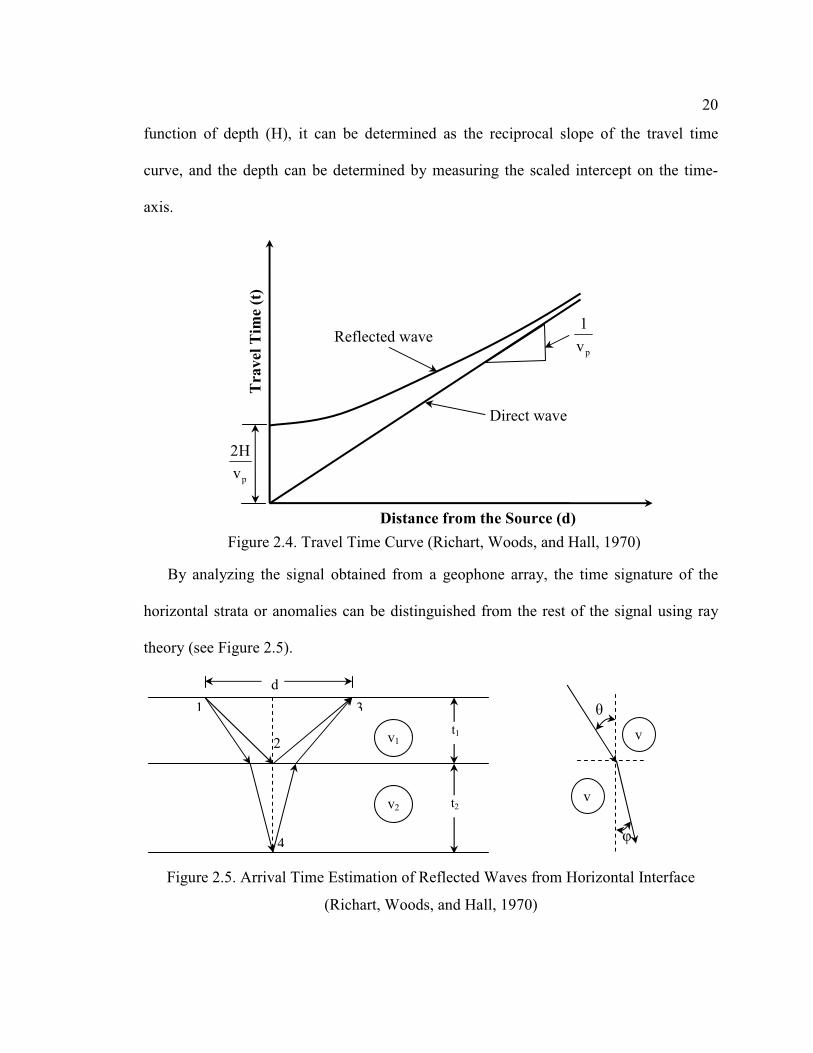
travel time curves (see Figure 2.4). For layers in which the wave velocity ( pv ) is not a
20
function of depth (H), it can be determined as the reciprocal slope of the travel time
curve, and the depth can be determined by measuring the scaled intercept on the time-
axis.
By analyzing the signal obtained from a geophone array, the time signature of the
horizontal strata or anomalies can be distinguished from the rest of the signal using ray
theory (see Figure 2.5).
Figure 2.5. Arrival Time Estimation of Reflected Waves from Horizontal Interface
(Richart, Woods, and Hall, 1970)
v
v
θ
φ
pv
1
Direct wave
Reflected wave
pv
H2
Figure 2.4. Travel Time Curve (Richart, Woods, and Hall, 1970)
Travel Tim
e (t)
Distance from the Source (d)
v1
v2
1 3
2
4
d
t1
t2

21
The time taken by wave-123 to reach 3 = 1
2
1
2
v
t2
d
2
+
and the time taken by wave-143 to reach 3 = 1
2
1
2
2
2
2
v
ttant2
d2
cosv
t2+
−
+
ϕ
ϕ
where,
v1 = wave velocity in layer 1
v2 = wave velocity in layer 2
t1 = thickness of layer 1
t2 = thickness of layer 2
and φ, θ is defined from the Snell’s law:
2
1
v
v
sin
sin=
ϕθ
,
There are also some disadvantages of the P-wave reflection. One major disadvantage
is that reflected P-waves arrive at the geophones after they have been excited by direct
waves (Gruber, and Rieger, 2003). Excitation of the geophones results in undesirable
vibrations with a slow dying rate and thus contaminates signals coming from reflections
from targeted anomalies, making the methods using first arrivals disadvantageous.
Another problem with P-waves is that they carry just 7% of the total energy, with the
remainder being lost to attenuation from traveling in soil media; thus, signals become
weaker as they are collected further from the source of generation.

22
2.5.2 Wavelet Analysis
2.5.2.1 Continuous Wavelet Transformation (CWT)
Wavelet analysis is a relatively new technique that can be applied to dynamic soil
response data to study signals in the time and frequency domains simultaneously. Kaiser
(1994) defined the wavelet transformation as, “…the convolution between a function
known as wavelet and the original signal.” A function, defined as a mother wavelet Ψ(t),
is required before performing a wavelet transformation. This function must be well
defined, localized in time and frequency domains, and should have a zero mean (Kaiser,
1994). There are many types of mother wavelets developed for purposes such as time
series analysis, dynamic data analysis, de-noising signals, image processing, and speech
recognition (Walker, 1999) and will be discussed later in this chapter.
A wavelet )(t,a τψ at time location t, scale a and integration variable τ is given by
the following equation (Walnut 2002):
=)(t,a τψa
1ψ
τ−a
t (2.2)
Continuous wavelet transform (CWT) WΨx of any signal x(t) with wavelet
)t(ψ having range of scales a is defined as follows (Walnut 2002):
∫+∞
∞−
= )()(xxW t,a*
t,a τψτψ τd (2.3)
where )(t,a* τψ is the complex conjugate of )(t,a τψ , t,axWψ is the wavelet coefficient,
and a is the scale of a wavelet that is the inverse function of frequency. To demonstrate
the functionality of scale, sine waves with different scales are plotted in Figures 2.6 (a)
through (c). The higher value of scale results in a more compressed wave and also

23
frequency has increased. Thus from Figure 2.6 it is evident that scale is inversely related
to radian frequency of sine functions.
-1.5
-1
-0.5
0
0.5
1
1.5
0 1 2 3 4 5 6 7
Time(t)
Sin(t)
-1.5
-1
-0.5
0
0.5
1
1.5
0 1 2 3 4 5 6 7
Time(t)
Sin(2t)
-1.5
-1
-0.5
0
0.5
1
1.5
0 1 2 3 4 5 6 7
Time(t)
Sin(4t)
Figure 2.6. Sine Function with Different Scales
In the case of wavelets the scale works in the same way as in the example of sine
waves shown in Figure 2.6. A db2 wavelet was plotted with different scales and is shown
in Figure 2.7. It is clear from the plots that a small value of scale results in a more
compressed wavelet and thus has a higher frequency content than the mother wavelet.
f=sin(t) ; a=1 f=sin(2t) ; a=1/2
f=sin(4t) ; a=1/4
a) Sine Function with scale a = 1 b) Sine Function with scale a = 1/2
c) Sine Function with scale a = 1/4

24
0 0.5 1 1.5 2 2.5 3-1.5
-1
-0.5
0
0.5
1
1.5
2
0 0.5 1 1.5 2 2.5 3-1.5
-1
-0.5
0
0.5
1
1.5
2
0 0.5 1 1.5 2 2.5 3-1.5
-1
-0.5
0
0.5
1
1.5
2
Figure 2.7. db2 Wavelet Function with Different Scales
From the Figure 2.7 it can also be concluded that in the wavelet analysis, the scales
can be related to the frequency of the wavelet and thus can be related to the frequency of
the signal. To compute the frequency related to the scale, the center frequency, Fc , of the
mother wavelet is computed. The center frequency is determined from the power spectral
density (PSD) plot of the mother wavelet. The frequency corresponding to the highest
power peak in the PSD plot is assigned as the center frequency of the mother wavelet.
For a given wavelet with scale a, its center frequency is also scaled by the factor Fc/a. If
the sampling period of the data ∆ is also considered, then the frequency corresponding to
the wavelet of certain scale a is given as:
∆=
.a
FF c
a (2.4)
Ψ(t)
Time (t)
Time (t) Time (t)
Ψ(t)
Ψ(4t
f=Ψ(4t) ; a=1/4
f=Ψ(2t) ; a=1/2 f=Ψ(t) ; a=1
c) Wavelet with scale a = 1/4
b) Wavelet with scale a = 1/2 a) Wavelet with scale a = 1

25
Thus, a higher scale represents low frequency and a low scale represents a high
frequency.
The CWT process can be regarded as an integration over the time length of the
original signal x(t) multiplied by a scaled wavelet. Equation (2.3) represents the
mathematical expression of this process. This process produces wavelet coefficients that
are a function of scale and time location. The step by step procedure of CWT process is
explained below.
1. Select a mother wavelet.
2. Select the scale range. This step identifies the frequency range of interest because
scales are related to the frequencies.
3. Select the scale interval. This step determines the scale values to be used in the
CWT process.
4. Take the wavelet with the initial value of scale and compare it to a section at the
start of the original signal x(t) (Figure 2.8). Calculate the wavelet coefficient from
Equation (2.3).
5. Shift the scaled wavelet to the new time position and calculate the wavelet
coefficients (Figure 2.9). This process is continued for the full length of the
signal.
6. Scale the mother wavelet according to the scale interval and the scale range.
7. Repeat steps 4 and 5.
8. The wavelet coefficient is then plotted either as a three dimension plot or as a
contour plot.

26
Figure 2.8. Place the Scaled Wavelet at the Signal Origin and Calculate Wavelet Coefficient
Figure 2.9. Shift the Scaled Wavelet to New Time Location and Calculate Wavelet Coefficient
The analyzing wavelet that correlates with the properties of the original time
varying signal, x(t), provides a larger value of the wavelet coefficient, or vice-versa.
Because the seismic signal varies rapidly in the time domain, its time-frequency plot is
expected to have considerable undulation as presented in Figure 2.10. Figure 2.10(a)
presents the three dimensional plot of wavelet coefficients and Figure 2.10(b) presents
the contour plot of the same data. Due to undulations in the three dimensional plot, all
features are difficult to interpret. However, the contour plot provides an effective way to
study all features. Thus, in this research, contour plots were used to study the signals
50 100 150 200 250 300-0.6
-0.4
-0.2
0
0.2
0.4
Sample#
X
Wavelet of scale a
50 100 150 200 250 300-0.6
-0.4
-0.2
0
0.2
0.4
Sample#
X
Wavelet of scale a

27
rather than three dimensional plots. In Figure 2.10(a), the undulations are plotted as
ripples in the contour plot. In the analysis, these ripples are referred as undulations as
they are crests and troughs in the three dimensional plot as indicated in Figures 2.10(a)
and 2.10(b).
(a) Three Dimensional Wavelet Coefficient Plot
High Coefficient
100 200 300 400 500 600 700 800 900 1000 1100 1
8
15
22
29
36
43
50
57
64
71
78
85
92
99
106
113
120
127
20
40
60
80
Low Coefficient
(b) Contour Plot of Wavelet Coefficients
Figure 2.10 Three Dimensional Wavelet and Contour Wavelet Plots
Sample# Scale
Sample#
Sca
le
Undulations
Each light contrast region represents a
peak and dark contrast represent trough
in three dimensional plot. This feature is
referred as undulation in the data analysis

28
A contour plot can be used to extract information both in global time and in the
frequency domain efficiently and accurately. To demonstrate the functionality of wavelet
transformations, a synthetic signal of known characteristics presented in Figure 2.11 and
defined by Equation (2.5) is analyzed. The wavelet coefficient map is generated using the
wavelet toolbox of MATLAB®
7.0.
x(t) = 0 0.0<t<0.2 (2.5)
= Sin(40 t) 0.2<t<1.0
= 0 1.0<t<2.6
= Sin(10 t) 2.6<t<3.1
= 0 3.1<t<3.2
0 0.5 1 1.5 2 2.5 3-1
-0.8
-0.6
-0.4
-0.2
0
0.2
0.4
0.6
0.8
1
Time (seconds)
Am
plitu
de
(m
)
Figure 2.11. Synthetic Signal
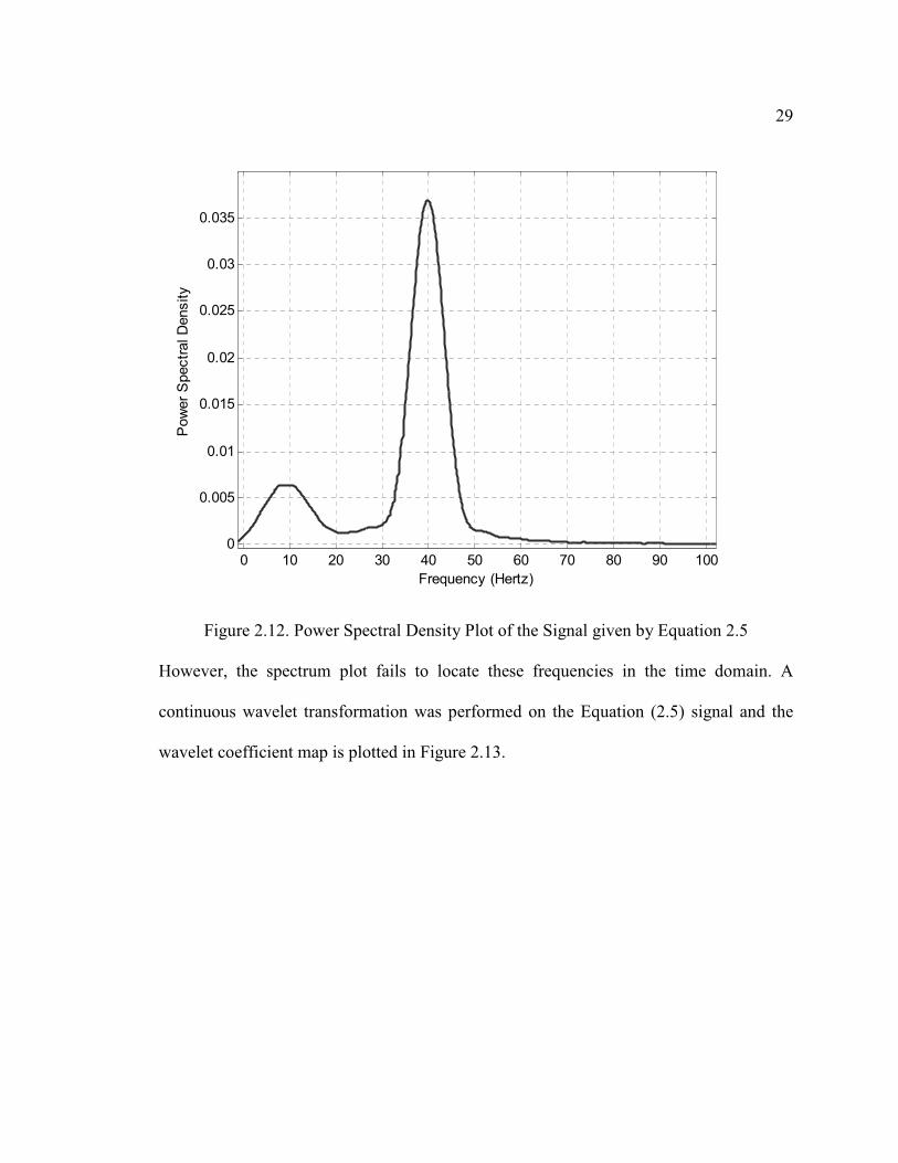
The signal defined by Equation (2.5) consists of two different frequencies of 40
hertz and 10 hertz respectively. Thus, the power spectral density of this signal consists of
two spikes at 10 and 40 hertz (Figure 2.12).
29
0 10 20 30 40 50 60 70 80 90 1000
0.005
0.01
0.015
0.02
0.025
0.03
0.035
Frequency (Hertz)
Pow
er
Spectr
al D
ensity
Figure 2.12. Power Spectral Density Plot of the Signal given by Equation 2.5
However, the spectrum plot fails to locate these frequencies in the time domain. A
continuous wavelet transformation was performed on the Equation (2.5) signal and the
wavelet coefficient map is plotted in Figure 2.13.

30
Figure 2.13 Wavelet Coefficient Map
Figure 2.13 presented two distinct regions of high color contrast that also corresponds
to the presence of the non-zero signal in that time range. Also, in the high contrast
regions, the maximum color contrast occurs at different scales. In the peak strength
region 1, the highest color contrast occurs around scale 71, corresponding to high
frequency presence in the corresponding portion of the signal. However, in the peak
strength region 2 the highest contrast occurs around scale 120, corresponding to low
frequency presence in the corresponding portion of the signal. Thus, it can be concluded
from Figure 2.11 that a wavelet coefficient map is able to provide information about the
frequency variation in time and can be used to detect reflected waves from any cavity or
obstacle that arrives later than the signal from the incident wave directly from the source.
In the field, horizontal layers of soil or any obstacles and anomalies reflect incident
High contrast region
represent the
presence of non-zero
value in signal.
Peak strength region 1
Peak strength region 2
Sca
le
Sample #

31
waves. In addition to wavelet transformation, the signal can also be processed through
low pass or high pass filters, depending on the signal and site characteristics, to identify
the reflected wave data. The wavelet transformation can then be applied to obtain a map,
as shown in Figure 2.13, to determine shape and size of any anomalies present in the soil
media.
2.5.2.2 Wavelet Families
In the research the affect of different type of wavelets on the continuous wavelet
transformation (CWT) was investigated and was utilized in the development of a protocol
for processing of seismic wave data for void detection. The CWT process depends
primarily on the selection of mother wavelet. It is a very important step in wavelet
analysis because an appropriate mother wavelet will produce the time-frequency plot
with distinct features that could be used for analyzing the signal properties. Wavelets are
broadly divided into small groups, known as wavelet families. Classification of wavelet
families is based on several criteria (Daubechies, 1992). The main criteria are:
• The support width of the mother wavelet function )(t,a τψ
• The speed of convergence to zero of the wavelet functions.
• The time t or frequency at which function value goes to infinity.
• The symmetry of the mother wavelet function that is useful in avoiding de-
phasing of the original signal.
• The number of vanishing moments for )(t,a τψ that is useful for compression
procedure of signals or images.
32
• The regularity of the mother wavelet function )(t,a τψ that is useful in smoothing
the reconstructed signal and for the estimated function in nonlinear regression
analysis.
Table 2.1 lists several wavelet families that are extensively used in signal and image
processing.
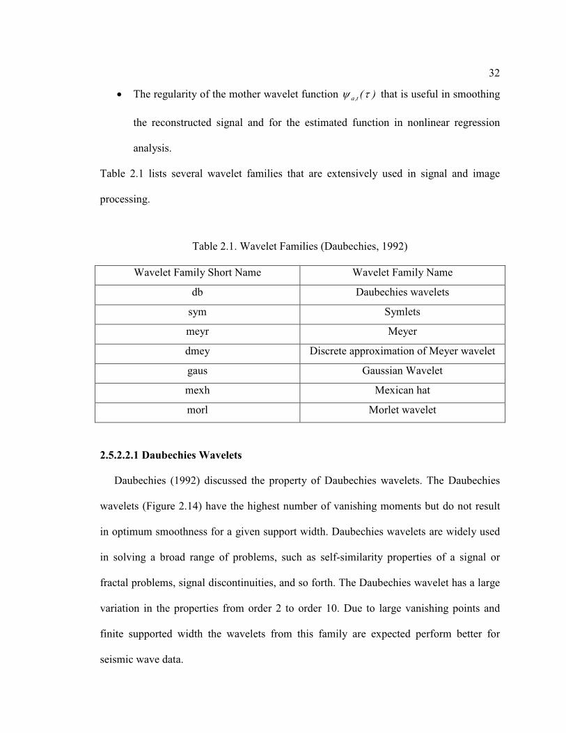
2.5.2.2.1 Daubechies Wavelets
Daubechies (1992) discussed the property of Daubechies wavelets. The Daubechies
wavelets (Figure 2.14) have the highest number of vanishing moments but do not result
in optimum smoothness for a given support width. Daubechies wavelets are widely used
in solving a broad range of problems, such as self-similarity properties of a signal or
fractal problems, signal discontinuities, and so forth. The Daubechies wavelet has a large
variation in the properties from order 2 to order 10. Due to large vanishing points and
finite supported width the wavelets from this family are expected perform better for
seismic wave data.
Table 2.1. Wavelet Families (Daubechies, 1992)
Wavelet Family Short Name Wavelet Family Name
db Daubechies wavelets
sym Symlets
meyr Meyer
dmey Discrete approximation of Meyer wavelet
gaus Gaussian Wavelet
mexh Mexican hat
morl Morlet wavelet

33
0 1 2 3
-1
0
1
0 2 4-1
0
1
0 2 4 6
-0.5
0
0.5
1
0 2 4 6 8-1
0
1
0 5 10-1
0
1
1
0 1 2 3 0 2 4-1
0 2 4 6 0 2 4 6 8-1
0 5 10
-1
0
1
0 5 10 15
-1
-0.5
0
0.5
0 5 10 15-1
-0.5
0
0.5
0 5 10 15-1
-0.5
0
0.5
Figure 2.14. Daubechies Wavelet family (Daubechies, 1992)
2.5.2.2.2 Symlet Wavelet Family
The Symlet wavelets (Figure 2.15) have the greatest number of vanishing points for a
given supported width and are highly symmetric (Daubechies, 1992). Symlet wavelet
applications are the same as the Daubechies wavelet applications. Due to very high
vanishing points for a supported length, these wavelets are expected to extract minor
details of the signal that include noise embedded in the signal.
0 1 2 3
-1
0
1
0 2 4
-1
0
1
0 2 4 6-1
0
1
0 2 4 6 8
-1
0
1
0 5 10
-0.5
0
0.5
1
0 1 2 3 0 2 4 0 2 4 6 0 2 4 6 8
0 5 10
-1
0
1
0 5 10 15
-0.5
0
0.5
1
0 5 10 15
-1
-0.5
0
0.5
0 5 10 15
-0.5
0
0.5
1
Figure 2.15. Symlet Wavelet Family (Daubechies, 1992)
2.5.2.2.3 Meyer Wavelet
Daubechies (1992) provides the detail discussion on Meryer Wavlet. Meyer wavelet
(Figure 2.16) is orthogonal, biorthogonal, symmetric, and infinitely derivable. The Meyer
db7 db8 db9 db10
db2 db3 db4 db5 db6
sym2 sym3 sym4 sym5 sym6
sym7 sym8 sym9 sym10

34
wavelet is widely used for data mining processes and for interpreting
electroencephalography signals. The Meyer wavelet can be used to process the seismic
wave data, because the shape of this wavelet resembles surface waves traveling in media
and thus correlates with the signal properties and produce high resolution time-frequency
maps. However, if data is contaminated with ambient noise, correlation will result in
undesired high frequency ripples in a time-frequency map.
-8 -6 -4 -2 0 2 4 6
-0.8
-0.6
-0.4
-0.2
0
0.2
0.4
0.6
0.8
1
Figure 2.16. Meyer Wavelet (Daubechies, 1992)
2.5.2.2.4 Mexican Hat Wavelet
Mexican hat wavelets are also discussed by Daubechies, (1992). Mexican hat
wavelets (Figure 2.17) are computed from the second derivative of the Gaussian
probability density function. Since the Gaussian probability density function is
symmetric, this wavelet is also symmetric, but not orthogonal. The Mexican hat wavelet
can be used for continuous wavelet transformation, but lacks the ability to perform
discrete wavelet transformation. This wavelet has small number of vanishing point. Thus,
this wavelet is expected to eliminate the noise embedded in the seismic signal data but it
might also eliminate some signal details.
35
-8 -6 -4 -2 0 2 4 6 8
-0.2
0
0.2
0.4
0.6
0.8
Figure 2.17. Mexican Hat Wavelet (Daubechies, 1992)
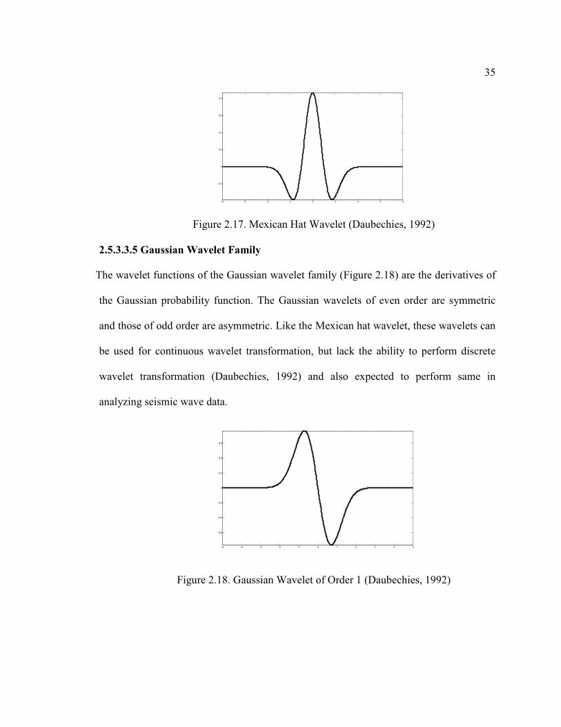
2.5.3.3.5 Gaussian Wavelet Family
The wavelet functions of the Gaussian wavelet family (Figure 2.18) are the derivatives of
the Gaussian probability function. The Gaussian wavelets of even order are symmetric
and those of odd order are asymmetric. Like the Mexican hat wavelet, these wavelets can
be used for continuous wavelet transformation, but lack the ability to perform discrete
wavelet transformation (Daubechies, 1992) and also expected to perform same in
analyzing seismic wave data.
-5 -4 -3 -2 -1 0 1 2 3 4 5
-0.6
-0.4
-0.2
0
0.2
0.4
0.6
Figure 2.18. Gaussian Wavelet of Order 1 (Daubechies, 1992)

36
2.6 Numerical Simulation of Wave-propagation in Elastic Media
Richart, Woods, and Hall (1970) investigated the wave propagation phenomenon in
elastic media and determined that wave propagation in elastic media can be approximated
in two dimensions by assuming that the wave propagation occurs in one plane and there
is no interference from the waves reflected in the lateral direction. This is a valid
assumption due to the fact that a point source in an elastic half space creates a
hemispherical wavefront with the material particles vibrating either along the zenith or
the radial direction of the wave motion. This prevents any interference between the waves
propagating in planes through the source and at different azimuth angles (Figure 2.19).
Figure 2.19. Surface Wave Front (Richart, Woods, and Hall 1970)

37
In two dimensions, the equations of motion of an elastic wave can be written as Richart,
Woods, and Hall (1970):
yx
u)G(
y
vG
x
v)G(
t
v
yx
u)G(
y
uG
x
u)G(
t
u
∂∂∂
++∂∂
+∂
∂+=
∂∂
∂∂∂
++∂
∂+
∂
∂+=
∂
∂
2
2
2
2
2
2
2
2
2
2
2
2
2
2
22
22
λλρ
λλρ
where,
ρ is the density of the elastic medium,
u = Displacement in x-direction.
v = Displacement in the y-directions,
t = time and
λ ,G = Lame’s constants.
Equation (2.6) and (2.7) is an elliptical, partial differential equation which can be
solved using the finite difference method (Kreyszig, 2005). The domain is discretized
into finite grids and boundary conditions are applied. Loading is simulated using a point
source acting on the surface of infinite stratified elastic media. In wave propagation
problems, the element dimensions are chosen by considering the highest frequency for
the lowest velocity wave. Large grid dimensions filter high frequencies, whereas very
small element dimensions introduce numerical instability and require considerable
computational resources (Schechter, Chaskellis, Mignogna, and Delsanto 1994). The time
increment is carefully chosen to maintain numerical stability and accuracy. Numerical
instability may cause the solution to diverge if the time increment is too large, whereas a
very short time increment can cause spurious oscillations, also known as Gibb’s
phenomenon. Schechter, Chaskellis, Mignogna, and Delsanto (1994) also determined
conditions which ensure that finite difference simulation can accurately predict the wave
(2.6)
(2.7)

38
propagation in elastic half-space and ensure numerical stability. For numerical stability,
the time step, ∆t is chosen by the von-Neumann stability criterion. In the case of finite
difference equations, this criterion yields:
2
t
2
l vvt
+
ε≤∆ (2.8)
where,
ε = lattice or grid size,
vl = longitudinal wave velocity, and
vt = transverse wave velocity.
When the boundary conditions are imposed, the finite difference equation for
displacements u and v at time t+∆t is given by Schechter, Chaskellis, Mignogna, and
Delsanto (1994):
)j,i,t(u)j,i(c)j,i,t(u)j,i(c)j,i,t(u)j,i(c
)j,i,t(u)j,i(c)j,i,t(u)j,i(c)j,i,t(u)j,i(c
)j,i,t(u)j,i(c)j,i,t(u)j,i(c)j,i,t(u)j,i(c
)j,i,t(v)j,i(c)j,i,t(v)j,i(c)j,i,t(v)j,i(c
)j,i,t(v)j,i(c)j,i,tt(v)j,i(c)j,i,t(v)j,i(c)j,i,tt(v
)j,i,t(v)j,i(c)j,i,t(v)j,i(c)j,i,t(v)j,i(c
)j,i,t(v)j,i(c)j,i,t(v)j,i(c)j,i,t(v)j,i(c
)j,i,t(v)j,i(c)j,i,t(v)j,i(c)j,i,t(v)j,i(c
)j,i,t(u)j,i(c)j,i,t(u)j,i(c)j,i,t(u)j,i(c
)j,i,t(u)j,i(c)j,i,tt(u)j,i(c)j,i,t(u)j,i(c)j,i,tt(u
111
11111
1111
111
1
111
11111
1111
111
1
151413
121110
987
654
321
151413
121110
987
654
321
−+−+++
++−++−−+
+−+++++
−+++−+
++−+=+
−+−+++
++−++−−+
+−+++++
−+++−+
++−+=+
∆∆
∆∆
The finite difference equations (2.9) and (2.10) utilize a central difference scheme in
the spatial domain, and leapfrog time iterations in the time domain. To impose continuity
of stresses and displacements across interfaces and boundaries of four cells surrounding a
(2.9)
(2.10)

39
cross point (i,j), a rigorous cross point formulation makes it possible to use the same
finite difference equations by making changes in weights, c(i,j). The c(i,j) are the weights
that help to validate solutions at each interior node, as well as boundary nodes, and
depend on the material properties of the four cells surrounding the node point (i,j) as
shown in Fig 2.20.
Figure 2.20. Sample Grid and Cells
There are many finite difference software currently available that can solve wave
propagation equations in two dimensional space. Wave2000®
Pro Version 2.2 is one one
of these software packages for computational ultrasonics (elastic wave propagation) and
utilizes the above-mentioned finite difference scheme for calculating approximate
solutions to wave equations in 2-Dimensional domain. Wave2000®
computes the full
elastic wave solution in an arbitrary two-dimensional domain subjected to specified
acoustic sources. The software not only simulates the complete spatial and time-
dependent acoustic solution, but also simulates measurements in a variety of source and
(i+1,j)
(i-1,j-1)
(i-1,j)
(i,j+1) (i+1,j+1)
(i,j-1) (i+1,j-1)
(i-1,j+1)
I II
III IV

40
receiver configurations. It is user friendly, has an extensive material library and
incorporates a wide range of source types that includes line source, point source, and
sphere source along with a wide variety of source waveforms. Other features of this
software include infinite boundary condition modeling, free boundary condition
modeling, and an ASCII export data facility. The software also offers a user friendly GUI
and helpfile. Due to such flexibility and wide range of applicability, Wave2000®
Pro
Version 2.2 was used in this research.
2.7 Summary
The exploration of the sub-surface tomography is an important part of planning and
designing structures. The currently available techniques for quick and efficient detection
of the tomographical features can vary widely in feasibility, cost-to-benefit ratio,
applicability, and effectiveness (Dobecki and Upchurch, 2006). Among these techniques,
the seismic wave techniques have been found to be successful in determining the sub-
surface soil properties (Seed, 1957). This chapter summarized fundamentals of wave
propagation in elastic media and seismic wave methods currently available for profiling
sub surface tomography, including void detection. Also included were the reviews of
wavelet fundamentals analysis and different types of wavelets; along with the finite
difference method basics that are used for numerically simulating wave propagation in
stratified and voided soil media.

41
Chapter 3
Testing Program
3.1 Introduction
Seismic wave tests require specialized electronic data acquisition and instrumentation
common to seismic ground motion testing equipment. In addition, specialized data
processing software is needed to process the acquired data. Each component of the
equipment and each of the commercially available software packages used in this
research is described in detail in this chapter. The data acquisition setup requires a
portable computer, a signal analyzer, and a significant number of horizontal and vertical
geophones. This chapter includes a description of the data acquisition system, software
used for acquisition and data processing, and techniques used in data processing and
experimental test setups. This experimental program was designed to measure the vertical
response of the ground surface from the seismic tests conducted on the soil box. The
seismic tests include refraction test to determine the shear wave velocity distribution of
the soil media in the box and the tests conducted on the soil media with and without a
void. The data from the latter tests were analyzed to develop a void detection scheme.
3.2 Data Acquisition System
The data acquisition system (Figure 3.1) used for the laboratory experiments consists
of: (1) Agilent TechnologiesTM
signal analyzer, (2) portable computer, (3) SN4- 4.5 Hz
digital grade geophones, (4) energy source, and (5) data acquisition software to interface

42
the signal analyzer with the portable computer. This data acquisition system is owned by
PennDOT and operated by the Penn State University.
3.2.1 Signal Analyzer
A Data Physics Agilent TechnologiesTM
VXI mainframe E8408A signal analyzer was
used in the present study. This signal analyzer is a 4-slot, C-size mainframe that contains
a one-slot E8491B with an IEEE-1394 PC link and one message-based VXI module. This
module allows a direct connection from the portable computer to the VXI mainframe via
a standard IEEE-1394 bus card. The VXI mainframe contains two Agilent E1433B, 8
channel, 196 Ksa/sec digitizers and digital signal processing (DSP) modules. The
E1433B module is a single slot, C-size, register based VXI module that includes DSP,
transducer signal conditioning, alias protection, digitization, and high-speed measurement
computation.
Figure 3.1 General Layout of the Data Acquisition System Setup
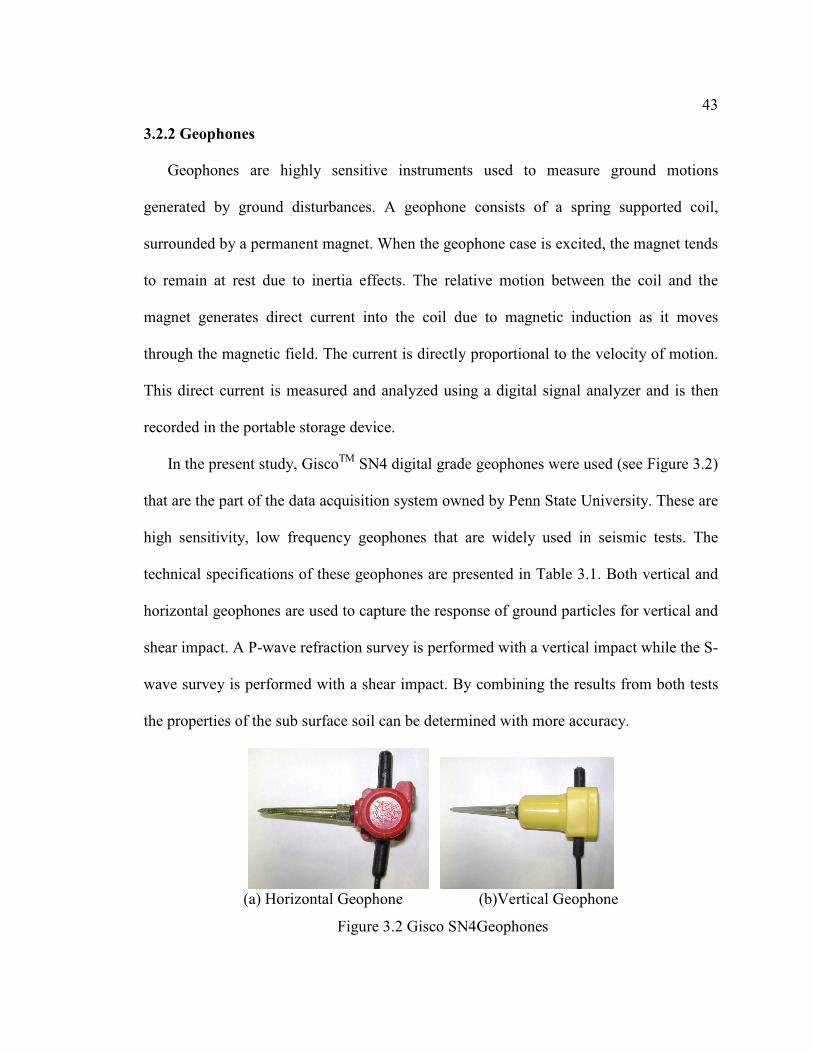
43
3.2.2 Geophones
Geophones are highly sensitive instruments used to measure ground motions
generated by ground disturbances. A geophone consists of a spring supported coil,
surrounded by a permanent magnet. When the geophone case is excited, the magnet tends
to remain at rest due to inertia effects. The relative motion between the coil and the
magnet generates direct current into the coil due to magnetic induction as it moves
through the magnetic field. The current is directly proportional to the velocity of motion.
This direct current is measured and analyzed using a digital signal analyzer and is then
recorded in the portable storage device.
In the present study, GiscoTM
SN4 digital grade geophones were used (see Figure 3.2)
that are the part of the data acquisition system owned by Penn State University. These are
high sensitivity, low frequency geophones that are widely used in seismic tests. The
technical specifications of these geophones are presented in Table 3.1. Both vertical and
horizontal geophones are used to capture the response of ground particles for vertical and
shear impact. A P-wave refraction survey is performed with a vertical impact while the S-
wave survey is performed with a shear impact. By combining the results from both tests
the properties of the sub surface soil can be determined with more accuracy.
(a) Horizontal Geophone (b)Vertical Geophone
Figure 3.2 Gisco SN4Geophones

44
Table 3.1. SN4- 4.5 Hz Digital Grade Geophone Specifications
Specifications Value
Natural frequency 4.5 Hz ± 0.5 Hz
With maximum tilt angle of 25o
Coil frequency 375 Ω
Open circuit damping 0.60
Sensitivity 28.8 v/m/s
Distortion <0.3%
Maximum coil excursion 4.0 mm
Moving Mass 11.30 mg
Diameter 26.0 mm
Height 37.0 mm
Weight 77.0 g
Operating Temp. Range -400 C to + 100
0 C
3.2.3 Energy Source
An energy source generates micro-seismic waves in the soil media. Methods include
the following:
1. A 4.5 kg to 7 kg (10 lb to 15 lb) sledge hammer is typically used in traditional
SASW tests.

45
2. A heavy drop weight that is able to generate lower frequency (high wavelength)
surface waves is used. The impact energy sources strike either a metallic or rubber
plate that serves to engage soil mass at the impact point and distribute the energy
to create a body wave rather than localized distorted energy.
3. A steady-state vibrator to generate single frequency waves. In a steady state
survey, seismic waves of a single frequency are generated by a vertically
oscillating vibrator.
The displaced shape of the ground due to steady state vibration can be approximated
by a sine curve that can be captured by a vertical geophone array. The wave length of a
Raleigh wave can easily be estimated as the distance between two successive troughs and
peaks. Once wavelength is calculated, the velocity of surface waves, which is
approximately equal to shear wave velocity, is computed using the principles of basic
wave mechanics. This shear velocity represents the average property of sub surface zone
of depth equivalent to the half wavelength of surface waves. By decreasing the
frequency, wavelength can be increased; thus increasing the depth of survey. For a
homogenous, isotropic, elastic half space, shear wave velocity is independent of depth,
but, for an elastic half space whose properties vary with depth, it is an effective method to
find the shear wave velocity distribution along depth.
3.2.4 Data Acquisition Software
A SignalCalc®
620 Dynamic Signal Analyzer was used as interface software for the
signal analyzer and the portable computer during the experiments. SignalCalc®
620
Dynamic Signal Analyzer is interface software for high-speed, industry standard HP VXI
digital signal processing hardware. This software was developed by Data Physics

46
Corporation and is part of the Data Physics signal analyzer equipment. This software can
interface with an unlimited number of input channels and can perform Fourier
transforms, real-time order analysis, real-time octave analysis, modal testing, amplitude
domain measurements (histograms), probability density plots, modal testing, disk record
and playback, and waterfall and spectrogram construction.
3.3 Laboratory Test Set Up
A wooden box of dimension 4.5m x 1.67m x 1.37m ( 64x65x51 ′′′′′′′ ) was constructed
to simulate a limited test sample of layered medium inside a laboratory. The dimensions
of the wooden box are shown in Figure 3.3.
(a) Wooden Test Box Layout
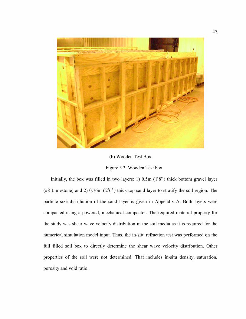
47
(b) Wooden Test Box
Figure 3.3. Wooden Test box
Initially, the box was filled in two layers: 1) 0.5m ( 81 ′′′ ) thick bottom gravel layer
(#8 Limestone) and 2) 0.76m ( 62 ′′′ ) thick top sand layer to stratify the soil region. The
particle size distribution of the sand layer is given in Appendix A. Both layers were
compacted using a powered, mechanical compactor. The required material property for
the study was shear wave velocity distribution in the soil media as it is required for the
numerical simulation model input. Thus, the in-situ refraction test was performed on the
full filled soil box to directly determine the shear wave velocity distribution. Other
properties of the soil were not determined. That includes in-situ density, saturation,
porosity and void ratio.
48
The soil box was initially filled till the intermediate partition (Figure 3.3(a)) and the
seismic tests were performed. The tests with this setup were conducted in two sets with
geophones at a spacing of 0.15m ( 6 ′′ ) and 0.203m (8 ′′ ) and a source offset of 0.254m
( 01 ′′ ) and 0.23m (9 ′′ ), respectively. The data from both test setups were processed using
the MATLAB®
7.0 programming platform and MATLAB®
7.0 wavelet toolbox. Time-
history plots and time-frequency plots for both test setups show that the near field effects
such as body wave interference and cylindrically spreading point source dominated the
signal, and thus, the arrival time of the three kinds of waves are indistinguishable. The
final tests were conducted on the full length of the box, filled in two different material
layers to minimize contamination from the near field effects. During preliminary tests, a
7.25 kg (16 lb) sledgehammer was utilized with a steel impact plate as an energy source.
This resulted in the generation of unnecessary echo in the soil box and contaminated the
signal. The energy source was varied to capture the effect of weight and frequency of
impact for testing in a soil box. The best results came from a 7.25 kg (16 lb)
sledgehammer and variations of impact force and plate type. A soft impact produced with
a small swing of the sledge hammer on a steel plate was used to generate low frequency
waves, and a hard impact produced with large swing of a rubber mallet was used to
generate a high frequency signal. The impact energy was not explicitly measured but data
was analyzed from the final tests to study the properties of the impact.
The test setup for void detection is illustrated in Figure 3.4. The data acquisition
system used in the study has the limitation of sixteen channels. Thus, the test was setup
with 0.305m (1′ ) spacing to cover the full length of the box. But the same test setup was
utilized to capture the vertical response of the top surface of the soil box with and without

49
a void. Thus to make room for the void, four channels were removed. The resulting test
set up consisted of 11 channels with a receiver spacing of 0.305m (1′ ) from channel one
to nine. Channel 10 is separated by 0.91m ( 3′ ) from channel 9 and 1.22m ( 4′ ) from
channel 11, as shown in figure 3.4. A void of 0.46m ( 61 ′′′ ) long, 0.91m ( 3′ ) wide, and
0.61m ( 2′ ) deep was excavated at a distance of 1.14m ( 93 ′′′ ) from the left edge of the
soil box. Initially the void of dimension 0.152m x 0.152m x 0.152m )1x1x1( ′′′ was
targeted. But as the void was excavated, the walls of the void were not stable enough and
were collapsing inside. Thus the void was excavated till the walls were stable. The final
size of the void was measured and used in the analysis. The void was finally covered with
1/4˝ plywood and a 4˝ soil was placed over the plywood (Figure 3.4(c)). The energy
source was placed at channel 1 so that the distance between the energy source and void
was maximized and near field effect was minimized.
Figure 3.4(a). Test Setup Scheme in Absence of Void

50
Figure 3.4(b). Test Setup Scheme for Void Detection
Figure 3.4(c). Void Detail (Section 1-1)
3.4 In-situ Shear Wave Velocity Determination: Refraction Test on Soil Box
The wave propagation phenomenon was simulated for voided and stratified regions,
using the finite difference method in the Wave2000Pro software. The Wave2000Pro
software requires shear wave velocity as an input for the numerical model. Thus only
shear wave velocity distribution was determined with a refraction test. To increase the
1
1
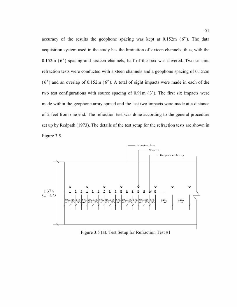
51
accuracy of the results the geophone spacing was kept at 0.152m ( 6 ′′ ). The data
acquisition system used in the study has the limitation of sixteen channels, thus, with the
0.152m ( 6 ′′ ) spacing and sixteen channels, half of the box was covered. Two seismic
refraction tests were conducted with sixteen channels and a geophone spacing of 0.152m
( 6 ′′ ) and an overlap of 0.152m ( 6 ′′ ). A total of eight impacts were made in each of the
two test configurations with source spacing of 0.91m (3′ ). The first six impacts were
made within the geophone array spread and the last two impacts were made at a distance
of 2 feet from one end. The refraction test was done according to the general procedure
set up by Redpath (1973). The details of the test setup for the refraction tests are shown in
Figure 3.5.
Figure 3.5 (a). Test Setup for Refraction Test #1

52
Figure 3.5 (b). Test Setup for Refraction Test #2
3.5 Summary
This chapter presents the details of the testing program, including details of the data
acquisition and instrumentation system, laboratory test setup for void detection, and setup
for the in-situ testing conducted for determining the shear wave velocity of the soil mass
in the soil box.

53
Chapter 4
Numerical Simulation
4.1 Introduction
The numerical simulation of surface wave propagation was completed with a finite
difference software program, Wave2000®
Pro Version 2.2. The objectives of the
numerical study were to simulate the wave propagation phenomenon in stratified and
voided elastic media and to investigate the affect of the voids on the vertical response of
the stratified elastic media. This chapter is a review of the parameters associated with
finite difference time domain (FDTD) simulation of wave propagation in elastic media,
and the numerical model used for the simulation of the soil box test.
4.2 Parameters for FDTD Simulation of Wave Propagation Phenomenon
The finite difference method is a powerful tool used to solve a large variety of
conventional partial differential equations. Due to the simplicity and applicability of this
method, finite difference is widely used for solving partial differential equations of wave
propagation in the time domain. In this study, Wave2000®
Pro Version 2.2 finite
difference software was used for numerical simulation. Wave2000®
Pro Version 2.2 is a
unique software package used for solving computational ultrasonic problems. It provides
solutions to a broad range of two dimensional ultrasound problems. With this software,
the problem domain and objects within the domain are specified in a PCX image file
format. The image data is composed of individual pixels that can have gray levels from 1
to 256 (0-255). Each pixel represents a single finite difference grid and its gray level

54
value represents a unique material assigned to that gray level. It is possible to construct
objects of any shape and size via the graphical user interface and assign different material
properties to these objects. The parameters that govern the ultrasonic simulations are: 1)
image size; 2) material properties; 3) boundary conditions; 4) source configuration; 5)
receiver configuration; 6) time step scale; 7) maximum frequency. These parameters are
briefly discussed below:
4.2.1 Image Size
Image size determines the magnitude and size of a problem and also determines the
computational resources requirement. Image size is determined by two parameters: (1)
physical dimension of the problem, and (2) desired image resolution. Physical dimension
is the actual size of the problem domain measured in millimeters and image resolution is
the number of pixels in one millimeter. Resolution of the image is directly proportional to
accuracy of the final results, but higher resolution results in high computational demands;
thus, a balance should be maintained between computational resources and desired
precision. For geophysics problems, the physical dimension of the problem is huge, as
compared with other types of ultrasonic problems. Therefore, in order to match the
computational demand of the problem with capabilities of available computational
resources, resolution of the image is kept low—around 0.2 pixels per millimeter.
4.2.2 Material Properties
The Wave2000®
Pro Version 2.2 package comes with a built-in material library that
contains details of properties of many materials that are used for general ultrasonic
problems. The software also allows for addition of user-defined materials to the library.

55
The software requires the material properties in order to calculate longitudinal wave
velocity and shear wave velocity, using the relationship shown below:
ρλ G2
v p+
= (4.1)
ρG
vs = (4.2)
where, λ and G are the Lame’s constants and ρ is the material density. For the numerical
simulation the shear wave velocity was directly determined by the refraction tests
conducted on the soil box.
4.2.3 Boundary Conditions
The user may input boundary conditions within the object, as well as at the external
four edges of the object. Three types of boundary conditions can be used:
1. Longitudinal mode fixed: This boundary condition acts as fixed condition for the
particle motion in the direction of the wave propagation.
2. Shear mode fixed: This boundary condition acts as fixed condition for the particle
motion in the direction perpendicular to the wave propagation direction.
3. Infinite boundary condition: This boundary condition is imposed on any of the
external four edges of the problem domain to make that side boundary appear as
an infinite medium matched to the material just inside the boundary of the object.
Infinite boundary condition is very useful in simulating geophysical problems.
4.2.4 Source Configuration
A source is used to generate ultrasonic disturbance in the problem domain. A source
can be placed inside the problem domain or at any external edges. The source waveform

56
can be manipulated using temporal functions, including continuous and pulsed sinusoids,
exponentially damped sinusoids, and sinusoids with a Gaussian time envelope. An
arbitrary source waveform can also be defined that allows incorporating actual ultrasonic
waveforms from an experiment into the simulation.
4.2.5 Receiver Configuration
A receiver is used to capture response of the medium at any desired location. Any
number of receivers can be defined inside the domain of the problem or at external edges
to measure displacement or velocity. Receiver measurements can be saved to file for
subsequent processing and analysis. The file contains both longitudinal and transverse
displacements made at the receiver location in ASCII format that can be easily imported
to a variety of signal processing software packages.
4.2.6 Time Step Scale
A time step scale parameter is utilized to control the time step of the simulation. The
software internally computes the time step, based on grid element size and wave
velocities within defined materials. However, this time step does not account for changes
required due to specific boundary conditions, attenuation settings, source signals, and
other model settings. Therefore, to ensure the stability of the simulation, the internally
computed time step is adjusted using a time step scale. The actual time step is then
determined by the product of the time step scale and internally computed time step.
4.2.7 Maximum Frequency
The maximum frequency parameter is an important parameter to calculate the
minimum wavelength and the resolving wavelength. The resolving wavelength and the
points/cycle determine the grid size of the numerical model. Maximum frequency is
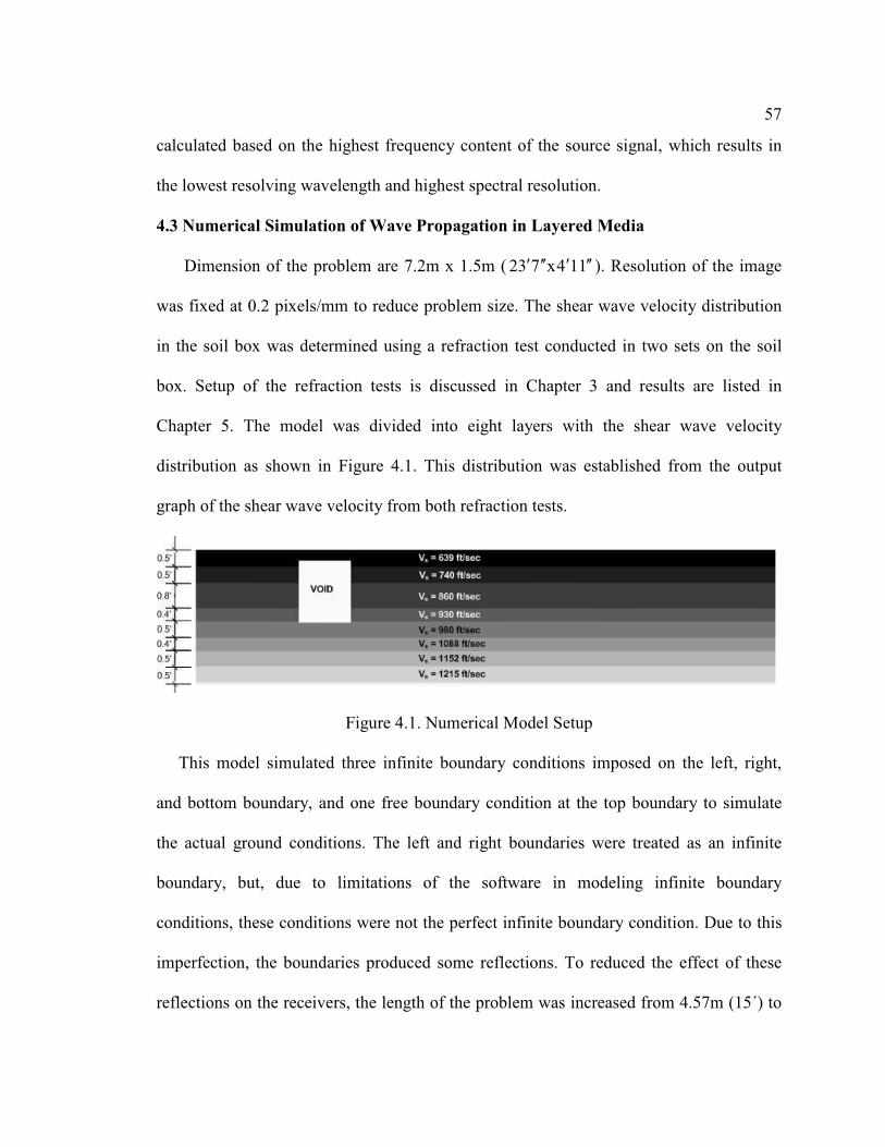
57
calculated based on the highest frequency content of the source signal, which results in
the lowest resolving wavelength and highest spectral resolution.
4.3 Numerical Simulation of Wave Propagation in Layered Media
Dimension of the problem are 7.2m x 1.5m ( 114x732 ′′′′′′ ). Resolution of the image
was fixed at 0.2 pixels/mm to reduce problem size. The shear wave velocity distribution
in the soil box was determined using a refraction test conducted in two sets on the soil
box. Setup of the refraction tests is discussed in Chapter 3 and results are listed in
Chapter 5. The model was divided into eight layers with the shear wave velocity
distribution as shown in Figure 4.1. This distribution was established from the output
graph of the shear wave velocity from both refraction tests.
Figure 4.1. Numerical Model Setup
This model simulated three infinite boundary conditions imposed on the left, right,
and bottom boundary, and one free boundary condition at the top boundary to simulate
the actual ground conditions. The left and right boundaries were treated as an infinite
boundary, but, due to limitations of the software in modeling infinite boundary
conditions, these conditions were not the perfect infinite boundary condition. Due to this
imperfection, the boundaries produced some reflections. To reduced the effect of these
reflections on the receivers, the length of the problem was increased from 4.57m (15΄) to

58
7.01 (23΄) so that reflections are delayed and had a minimum effect on the receivers.
Even though the length was increased, the reflections were not eliminated completely and
the effect could be seen in the time-frequency plot of the receivers. The loading pulse was
simulated using a point source function acting on the top surface given by Zerwer,
Cascante, and Hutchinson (2002):
)t(
tF)t(
22
b
ψπδ
+= (4.3)
where Fb alters the magnitude of the excitation; ψ controls the frequency content of the
excitation, and t represents time.
Source and receiver locations in the numerical model were the same as the geophone
locations in the soil box test (Figure 3.5). The test set up consisted of eleven receivers
with a receiver spacing of 0.3m (1′ ) from receiver 1 to 9. Receiver 10 is 0.914m (3′ )
from receiver 9 and 1.22m ( 4′ ) from the receiver 11. The source was at the same location
as receiver 1. To insure numerical stability of the simulation, the time step scale factor
was established as 0.9. During the simulation the source was active for 2.5ms and total
simulation time was 50ms. The source signal was analyzed in the frequency domain and
maximum frequency was established at 0.2 Khz, resulting in the grid size of 5 mm and 5
grids/pixel. The center of the void was placed at the same location as shown in Figure
3.4.

59
4.4 Summary
This chapter summarized the various aspects of numerical modeling of the wave
propagation problem in a soil box, using Wave2000®
Pro Version 2.2 software. All
parameters related to the numerical modeling and their applicability was discussed in
detail.

60
Chapter 5
Results and Discussion
5.1 Introduction
Seismic ground motion data requires specialized interpretation techniques to extract
required information about the ground medium because information from the propagation
of all types of waves is included. This chapter reviews techniques used in this study to
analyze the seismic test data collected from laboratory test in the soil box and a
corresponding numerical simulation. This chapter reviews the results from two refraction
tests conducted on soil media in a soil box to determine shear wave velocity profile of the
soil mass in the box and also the results from the wavelet analysis of the data from the
soil box seismic tests.
5.2 Data Processing
Data obtained from soil box tests were analyzed using the MATLAB®
7.0 wavelet
toolbox and MATLAB®
7.0 programming platform. Codes were written using the
MATLAB®
7.0 programming platform to plot the time-history of the signals from all
geophones to perform wavelet analysis and to construct time-frequency plots of the
geophone data. Data obtained from the refraction test was processed using
Seisimager®
2D, a data processing software for seismic refraction survey test data.

61
5.2.1 Data Processing Software
5.2.1.1 MATLAB® 7.0 Programming Platform and Wavelet Toolbox
MATLAB®
7.0 is a computing environment and programming language created by
Math Works, Inc. MATLAB®
7.0 that allows matrix manipulation, plotting of functions
and data, implementation of algorithms, graphic user interface creation, and interfacing
with programs in other languages. The programming platform comes with a built-in
library of functions for typical programming processes that would otherwise require
function call codes. MATLAB®
7.0 has a powerful base for input/output file processing
that makes it very efficient for reading data stored in ASCII format.
The MATLAB®
Wavelet Toolbox is a collection of built-in functions written on the
MATLAB®
7.0 Technical Computing Environment. This provides tools for analysis and
synthesis of signals and images, statistical applications, as well as wavelets and wavelet
packets within the framework of MATLAB®
7.0. In this study, the toolbox was used to
remove noise from the data and to construct a time-frequency plot of the signal to study it
in both time and frequency domains simultaneously.
5.2.1.2 Seisimager®2D
SeisImager®
2D from Geometrics, Inc. provides data processing and analysis for
refraction tests. It can perform comprehensive refraction modeling using ray tracing for
both P-wave and shear wave refraction surveys. The software reads seismic trace data
obtained from refraction survey tests in a general format for seismic data analysis, also
known as the SEG-2 or SEG-Y format. The signal analyzer exports data in ASCII format
that is then converted to SEG-2 format by the program IXSeg2Segy.

62
5.2.2 Data Processing Protocol
A step-by-step protocol was developed for data processing to ensure that information
regarding the soil medium could be efficiently extracted from seismic test data. The data
processing protocol is shown in Figure 5.1. Both numerical simulation and experimental
test data were processed using the same protocol.
Figure 5.1. Protocol for Data Processing
This data processing protocol includes two main steps: 1) removal of noise from the
raw data; 2) performs CWT on the processed data. MATLAB®
7.0 wavelet based inbuilt

63
functions were used for the noise removal from the seismic data. The second step consists
of several sub-steps:
i. Select a mother wavelet.
ii. Select a scale range and scale interval. Because scales are inversely related to
the frequency, this sub-step is based on the interested frequency range.
iii. Perform the CWT using the selected wavelet over the selected scale range
and interval. Codes were written in MATLAB®
7.0 to perform this sub-step.
iv. Construct time-frequency plots from the wavelet coefficients calculated from
CWT.
v. Accept the time-frequency plot if the features such as ripples and undulations
in the high and low scale regions are distinct. If the features are not distinct
select another mother wavelet and repeat the steps 2-5.
The selection of final mother wavelet relies on the user’s judgment as explained in
sub-step 5 of the second step. Thus, for different applications, different families of
wavelets might be more efficient.

64
5.3 Data Processing Results
5.3.1 In-situ Refraction Survey for In-situ Shear Wave Velocity Profile
The refraction tests were conducted on the soil box to determine the shear wave
velocity distribution in the media. This property was required for the numerical
simulation material model. Refraction test setup details are shown in Figure 3.5(a) and
3.5(b). Seismic data was analyzed using SeisImager®
2D. Results for the refraction tests
conducted in the soil box are shown in Figure 5.2(a) and 5.2(b). Results show some
localized variations in the shear wave velocity profile (Figure 5.2) that may be the result
of non-uniform compaction of the soil mass. For the numerical simulation material model
input, soil mass was divided into eight layers, with shear wave velocity and thickness, as
shown in Figure 4.1.
Figure 5.2 (a). Shear Wave Velocity Profile for Refraction Test #1 Conducted on Full
Length Soil Box
ft/sec
0.0' 1.0' 2.0' 3.0' 4.0' 5.0' 6.0' 7.0' 7.5'
Distance from the left edge of the soil box
C
Local shear wave
velocity variation

65
Figure 5.2 (b). Shear Wave Velocity Profile for Refraction Test #2 Conducted on Full
Length Soil Box
5.3.2 Wavelet Analysis of the Experimental Data
5.3.2.1 Analysis Using Different Wavelet Families
Seismic test data was analyzed using different wavelets from MATLAB®
7.0.
Wavelet toolbox built-in wavelet families were used to investigate the effect of different
types of wavelets on time-frequency maps. Selection of wavelets during the continuous
wavelet transformation is an important step in the data processing procedure. If the shape
of the mother wavelet is out of phase with the original signal then the different time-
frequency plot features (variation of wave strength in scales, time-localization of
frequency content) are not distinct (the contours are not clearly visible), resulting in high
smoothing. However, if the shape of the mother wavelet is in-phase with the signal, then
the time-frequency plot features are distinct and can be interpreted. Often, high
smoothing is not desired as it eliminates minor details of signals but no smoothing will
ft/sec
7.5' 8.5' 9.5' 10.5' 11.5' 12.5' 13.5' 14.5' 15'
Distance from the left edge of the soil box
C
Local shear wave
velocity variation
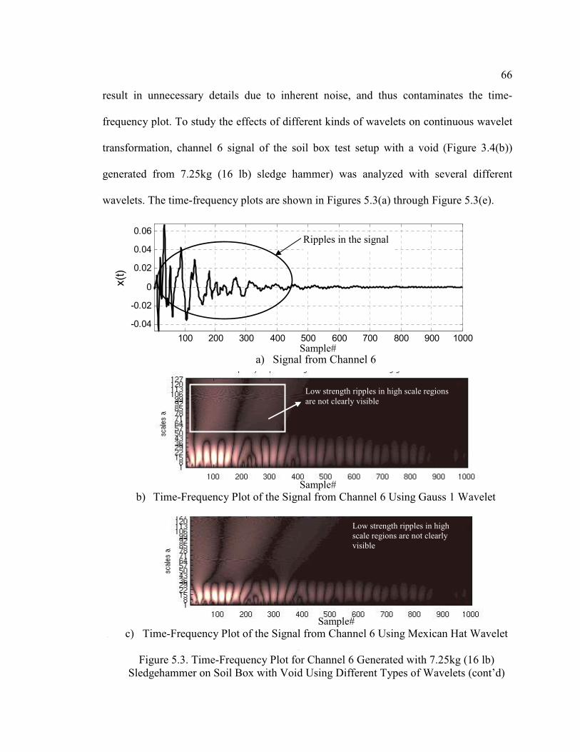
66
result in unnecessary details due to inherent noise, and thus contaminates the time-
frequency plot. To study the effects of different kinds of wavelets on continuous wavelet
transformation, channel 6 signal of the soil box test setup with a void (Figure 3.4(b))
generated from 7.25kg (16 lb) sledge hammer) was analyzed with several different
wavelets. The time-frequency plots are shown in Figures 5.3(a) through Figure 5.3(e).
100 200 300 400 500 600 700 800 900 1000
-0.04
-0.02
0
0.02
0.04
0.06
Sample#
x(t
)
a) Signal from Channel 6
b) Time-Frequency Plot of the Signal from Channel 6 Using Gauss 1 Wavelet
c) c) Time-Frequency Plot of the Signal from Channel 6 Using Mexican Hat Wavelet
d)
Figure 5.3. Time-Frequency Plot for Channel 6 Generated with 7.25kg (16 lb)
Sledgehammer on Soil Box with Void Using Different Types of Wavelets (cont’d)
Sample#
Low strength ripples in high scale regions
are not clearly visible
Low strength ripples in high
scale regions are not clearly
visible
Sample#
Sample#
Ripples in the signal

67
e) Time-Frequency Plot of the Signal from Channel 6 Using db1 Wavelet
f) Time-Frequency Plot of the Signal from Channel 6 Using Symlet2 Wavelet
g) Time-Frequency Plot of the Signal from Channel 6 Using db10 Wavelet
Figure 5.3. Time-Frequency Plot for Channel 6 Generated with 7.25kg (16 lb)
Sledgehammer on Soil Box with Void Using Different Types of Wavelets
The first two time-frequency plots (Figure 5.3(b) and 5.3(c)) were generated using the
Gaussian and Mexican hat wavelets. The supported width of these wavelets varies from
-∞ to +∞ and has a bell shape. However, the signal from the geophone is localized in
time, consists of numerous ripples, and is not smooth. Due to differences in the shape of
the original signal and the mother wavelet, the CWT eliminates minor details of the
Sample#
The peaks in low and high scale
regions are not distinct
Minor Details
The peaks in both high scale
and low scale regions are very
close to each other and thus are
not distinct
Minor Details
Clear low strength ripples in high
and low scale region.
Sample#
Sample#

68
signal, and thus high scale (scale 64-128) peaks are not distinct in the time-frequency
maps. db1 and symlet2 wavelets have small supported width and large vanishing points
for the supported width and their shape resembles the original signal. Due to the
similarity between the properties of the original signal and these wavelets, the CWT
resulted in minor details in the time-frequency maps including the noise embedded with
the system. These details contaminated the time-frequency map and made the data
interpretation task more difficult. A db10 wavelet was used in the final wavelet
transformation (Figure 5.3(f)) because the db10 mother wavelet shape resembles the
shape of the original geophone signal and also the properties of the signal. The db10
wavelet resulted in filtering of small ripples caused by noise in the time-frequency plots
and thus all the features of the signals in the high scale and low scale regions are distinct
(Figure 5.3(f)). Thus, this wavelet was used in the final data analysis of the signals from
soil box test with and without a void.
5.3.2.2 Wavelet Analysis of Soil Box Test Data
Seismic tests were conducted on the soil box shown in Figure 3.3(b). For these tests,
a soft impact produced with a small swing of the sledge hammer on a steel plate was used
to generate low frequency waves (frequency ≈10 hertz). Also, a hard impact produced
with a large swing of a rubber mallet was used to generate a high frequency (frequency
≈500 hertz) signal.
A surface wave traveling in an elastic media, with material properties as a function of
depth, experiences dispersion and material and geometric damping phenomenon.
Material and geometrical damping results in signal power loss that is directly
proportional to the distance traveled by the surface wave. In the absence of anomalies

69
like voids, surface waves do not encounter an obstruction in the wave path, therefore, any
observation made in a time-frequency plot of the receiver signal under such conditions
can be marked as a signature of surface wave damped and dispersive behavior. In the
setup shown in Figure 3.4(a) for the laboratory test without a void, channel 1 is at the
source location and was selected for data analysis because it provides the closet
approximation of the impact properties. However, the distance between the source and
channel 1 is insufficient to produce any damping or dispersive behavior. Therefore,
channel 10 was selected for analysis as it is located at the maximum distance from the
source. Thus, seismic waves can experience sufficient dispersion and damping
phenomenon before it reaches channel 10 and thus can be studied. Also, channel 4,
located near the center of the soil box, was selected for analysis to observe the change in
the dispersion and damping behavior as seismic waves travel across the box. The signals
from both channels 4 and 10 were analyzed in the time-frequency domain to study the
effects of dispersion and damping in order to mark the signature of dispersion and
damping behavior.
MATLAB®
7.0 was used to remove noise from the data, perform continuous wavelet
transformation analysis on the data, and construct time-frequency plots. Time-frequency
plots were generated with db10 wavelets for scales from 2 to 128 with a scale interval of
2. Time-frequency plots for channels 1, 4, and 10 are shown in Figure 5.4.

70
(a) Time-frequency Plot of Channel 1
(b) Time-frequency Plot of Channel 4
(c) Time-frequency Plot of Channel 10
Figure 5.4. Time-Frequency Plot for Channels 1, 4, and 10 Generated from 7.25kg (16 lb)
Sledgehammer on Soil Box without Void
Figures 5.4(a), 5.4(b) and 5.4(c) illustrate time-frequency plots of channels 1, 4, and
10 test setups without a void, and were generated using a 7.25kg (16 lb) sledgehammer.
Channel 4 and channel 10 signal time-frequency plot show uniform damped undulations
Sample#
Sample#
Sample#
No damp undulations present in this region
Damped undulation
Damped undulation
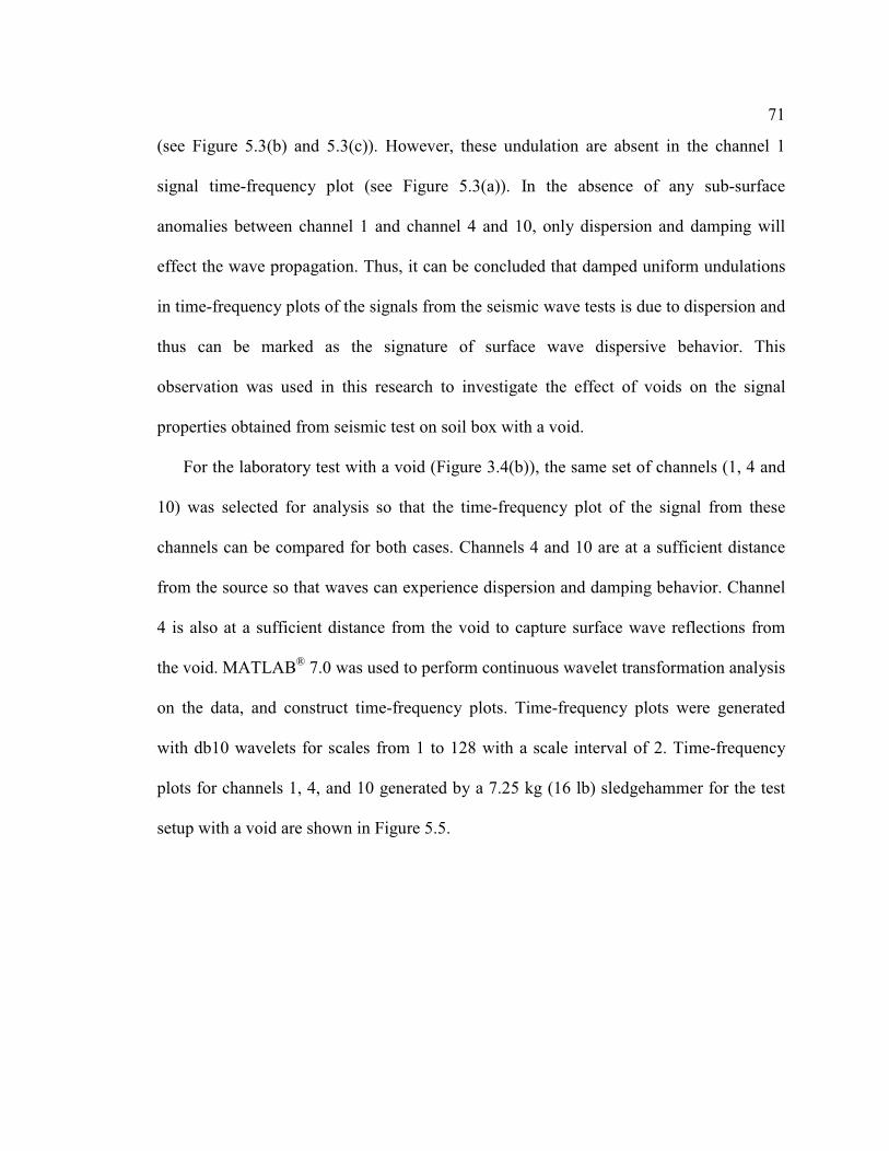
71
(see Figure 5.3(b) and 5.3(c)). However, these undulation are absent in the channel 1
signal time-frequency plot (see Figure 5.3(a)). In the absence of any sub-surface
anomalies between channel 1 and channel 4 and 10, only dispersion and damping will
effect the wave propagation. Thus, it can be concluded that damped uniform undulations
in time-frequency plots of the signals from the seismic wave tests is due to dispersion and
thus can be marked as the signature of surface wave dispersive behavior. This
observation was used in this research to investigate the effect of voids on the signal
properties obtained from seismic test on soil box with a void.
For the laboratory test with a void (Figure 3.4(b)), the same set of channels (1, 4 and
10) was selected for analysis so that the time-frequency plot of the signal from these
channels can be compared for both cases. Channels 4 and 10 are at a sufficient distance
from the source so that waves can experience dispersion and damping behavior. Channel
4 is also at a sufficient distance from the void to capture surface wave reflections from
the void. MATLAB®
7.0 was used to perform continuous wavelet transformation analysis
on the data, and construct time-frequency plots. Time-frequency plots were generated
with db10 wavelets for scales from 1 to 128 with a scale interval of 2. Time-frequency
plots for channels 1, 4, and 10 generated by a 7.25 kg (16 lb) sledgehammer for the test
setup with a void are shown in Figure 5.5.

72
(a) Time-frequency Plot of Channel 1
(b) Time-frequency Plot of Channel 4
(c) Time-frequency Plot of Channel 10
Figure 5.5. Time-frequency Plot for Channels 1, 4, and 10 Generated from 7.25kg (16 lb)
Sledgehammer on Soil Box with Void
Figures 5.5(a), 5.5(b) and 5.5(c) show channels 1, 4, and 10 time-frequency plot
generated with a 7.25kg (16 lb) sledgehammer on the soil medium with a void. The
channel 4 signal time-frequency plot shows the signature of dispersion behavior as
damped uniform undulations (see Figure 5.5(b)), the same as concluded from the seismic
Sample#
Sample#
No damp undulations present in
this region
Damped undulation
Low strength ripples
in high scale region
Damped undulation
No low strength ripples in high scale region as
observed in time-frequency map of channel 4 signal
The strength of
signal is
distributed from
low to high scale.

73
test in the soil box without a void. Unique low strength ripples in the high scale (low
frequency) region between samples 300 and 700 can also be observed in this time-
frequency plot. However, these low strength ripples are not present in the channel 4
signal time-frequency plot obtained from the soil box test without the void (Figure
5.4(b)). Therefore, it can be concluded that low strength and high scale ripples are
occurring due to the reflections from the surface from the void because it is the only
difference in both test setup and thus, can be marked as the signature of the void-like
anomaly. Channel 10 signal time-frequency plot (Figure 5.5(c)) also shows the same
damped uniform undulations as observed in the channel 10 signal time-frequency plot
(Figure 5.4(c)) obtained from the soil test without the void. However, low strength, low
frequency ripples as observed in the channel 4 signal time-frequency plot (Figure 5.5(b))
are absent. From this observation it can be concluded that the void or anomalies do not
disrupt the time-frequency spectrum of the signals from geophones placed after the void
or anomalies.
A final set of tests were conducted on the laboratory soil box test setup with a void. A
rubber mallet was used as the energy source. MATLAB®
7.0 was used to perform
continuous wavelet transformation analysis on the data and construct time-frequency
plots. Time-frequency plots were generated with db10 wavelets for scales from 1 to 128
with a scale interval of 2. Time-frequency plots for channels 1, 4, and 10 signal generated
by a rubber mallet for the test setup with a void are presented in Figures 5.6.

74
a) Time-frequency Plot of Channel 1
b) Time-frequency Plot of Channel 4
(c) Time-frequency Plot of Channel 10
Figure 5.6. Time-frequency Plot for Channels 1, 4, and 10 Generated from Rubber Mallet
on Soil Box with Void
Apart from the similarities, time-frequency plots of the signals generated using
rubber mallets also shows some different features from the plots generated using a 7.25kg
(16 lb) sledgehammer.
Sample#
Sample#
Sample#
The strength of signal is
concentrated in low
scale region.
No damp undulations present in this region
Damped undulation
Low strength ripples in
high scale region
Damped undulation
No low strength ripples in high scale region as observed in
time-frequency map of channel 4 signal

75
Figures 5.5(a) and 5.6(a) presents the time-frequency plots of the signal from channel
1, located at the source, generated by the 7.25kg (16 lb) sledgehammer and a rubber
mallet respectively. Under a 7.25kg (16 lb) sledgehammer the major portion of energy
lies between 2 to 85, however under the rubber mallet the maximum energy lays between
scales 2 to 57. Thus, impact from the rubber mallet produces waves with a major portion
of energy in the high frequency (low scale) region. However, the high frequency waves
have a higher attenuation rate than the low frequency waves (Zerwer, 2002). Thus, the
dispersion phenomenon decay at a higher rate in the plots generated using a rubber mallet
than in the plots generated using a 16 lb sledgehammer (Figure 5.5(b) and Figure 5.6(b)).
Channel 4 signal time-frequency plot generated by the rubber mallet (Figure 5.6(b))
shows the same characteristics as the channel 4 signal time-frequency plot generated by
the sledgehammer (Figure 5.5(b)). Also, these low strength, high scale ripples are absent
from the channel 10 signal time-frequency plot generated by the rubber mallet (Figure
5.5(c)) and time-frequency plot of channel 10 signal generated by the sledgehammer
(Figure 5.5(c)). Thus, time-frequency plots of channel 1, 4 and 10 signal generated with a
rubber mallet on the test setup with void (Figure 5.6(a), 5.6(b) and 5.6(c)) confirm the
conclusions from the data analysis of the signals generated with a 7.25kg (16 lb)
sledgehammer. From this data analysis, it can also be concluded that the dispersion or
damping behavior signature and void signature in the time-frequency domain do not
change with source weight.
5.3.3 Wavelet Analysis of the Numerical Simulation Data
Seismic tests conducted on the soil box were simulated using Wave2000®
Pro Version
2.2 and the receiver data was processed using the same protocol that was used for the

76
experimental test data. Time-frequency plots were generated with db10 wavelets for
scales from 1 to 128 with a scale interval of 2. Plots for receivers 1, 4, and 10 are shown
in Figure 5.7.
(a) Time-frequency Plot of Receiver 1
(b) Time-frequency Plot of Receiver 4
(c) Time-frequency Plot of Receiver 10
Figure 5.7. Time-frequency Plot of Receivers 1, 4, and 10 Generated from Numerical
Simulation
Sample#
Sample#
Sample#
No damp undulations present in this region
Damped undulation
Low strength ripples in
high scale region
Damped undulation
No low strength ripples in high scale
region as observed in time-frequency
map of channel 4 signal
Reflections from the boundary
Reflections from the boundary

77
Receiver 4 signal time-frequency plot (Figure 5.7(b) presents uniform undulations,
both in high scale as well as low scale regions. Geometric damping causes the surface
wave dispersion to decay in the low scale region, but the decay rate is less than the
decaying observed in the experimental result because the material damping was not
considered in the numerical model. The attenuation is a very complex phenomenon for
the wave propagation in the dispersive media and also difficult to measure
experimentally. Thus it was not considered in the research scope and was also neglected
in the numerical study. The time-frequency plot of receiver 4 presents a unique time-
frequency spectrum signature of voids as low strength ripples in the time-frequency
domain in the high scale (low frequency) region between sample 350 and 700, similar to
the experimental results, which is absent from channel 1 and channel 10 signal time-
frequency plot. This plot also shows the some reflections from the infinite boundaries that
are contaminating the plot. Since the material damping was considered in this simulation
these reflections were not absorbed by the material. These reflections were not present in
the experimental data time-frequency plot since the material had its inherent damping that
helped in the absorption of any reflection from the boundary. The receiver 10 signal time-
frequency plot consists of the dispersion behavior time-frequency signature but no low-
strength, high-scale signature of voids, which confirm the conclusions from the
experimental data analysis. This time-frequency plot has same reflections as receiver 4
time-frequency plot as infinite boundary could not eliminate them.

78
5.4 Summary and Discussion
This chapter presents and reviews the results from the processing of numerical
simulation and the soil box experiment data. Wavelet analysis was perform on the
seismic data using different wavelet families and after observing the resulted time-
frequency plot, db10 was selected for the final data analysis. The dispersion and damping
behavior was studied using the channel time-frequency plots and signature of this wave
phenomenon in time-frequency domain was established. The time-frequency plot of the
signal generated using a 7.25 kg (16 lb) sledgehammer in the absence of a void shows
damped uniform undulations from low to high scales. These damped uniform undulations
in time-frequency plot of the signals from the seismic wave tests, in the absence of any
other anomaly, were marked as the signature of surface wave dispersive behavior. The
time-frequency plot of the signal generated using 7.25 kg (16 lb) sledgehammer on the
soil box test in the presence of the void shows low strength ripples in the high scale
region apart from the dispersive behavior signature from low to high scales. These low
strength ripples in high scale region were marked as the signature of the void-like
anomaly. The plywood that covers the void would also effect the wave propagation but
its affect was not studied separately but only as a part of the void like anomaly. No
geophones were placed on the top of the void due to insufficient thickness of soil layer
over the plywood. However, it is expected that it would show the same characteristics as
the geophone signal placed after the void because the reflection from the vertical wall of
the void would not disrupt the signal. Finally, the effect of source weight on the time-
frequency map was investigated and was concluded that the dispersion or damping

79
behavior signature and void signature in time-frequency domain do not change with
source weight.
The observation made in this research is based on the seismic test conducted on the
soil box with a void of definite dimension. The size of the void was not varied to study its
effects. However a parametric study that investigates the effect of shape, size and depth
of the void on the time-frequency maps would be beneficial in the further development of
the proposed protocol.

80
Chapter 6
Summary and Conclusions
6.1 Summary
This research investigated the effect of void like anomaly on surface wave
propagation by studying the signal in the time-frequency domain using continuous
wavelet transformation. The study also investigated the effects of different type of
wavelets on the CWT and developed a protocol for processing of seismic wave data to
construct time-frequency plots. These time-frequency plots were investigated for the void
like anomaly detection. This research was conducted in several steps. The first step in the
research program was to develop a controlled experiment to study surface wave
propagation in voided soil media. A wooden box was constructed and filled with a
bottom gravel layer and top sand layers. A refraction test was conducted on the soil mass
in the wooden box to compute the in-situ shear wave velocity distribution. The result
from the refraction tests were used to create a material model and its spatial distribution
for the finite difference simulation to study the wave propagation in voided soil media.
Then, seismic tests were conducted on the soil box without a void to study the geophone
signal in the time-frequency domain. The data from this set of tests was set as reference
for the data analysis of tests conducted on the soil box with the void. Finally the void of
known dimension was excavated in the soil mass at a known location. Seismic test were
conducted with the same geophone setup as the test without the void. The data from this
set of tests was analyzed to study the effects of the void like anomaly on the geophone

81
response. The effect of source weight on the time-frequency map was investigated by
using a sledgehammer and rubber mallet. The numerical model was created only for the
investigating the surface wave propagation in voided soil mass.
6.2 Conclusions
Based on the research, the following conclusions are:
• Continuous wavelet transformation can be used to study the seismic data
signal properties localized in the time domain.
• The shape and the properties of the mother wavelet influence the CWT
process. If the shape of the mother wavelet is in-phase with the original signal
then the time-frequency plot features (variation of wave strength in scales,
time-localization of frequency content) are distinct and can be investigated.
However, if the shape of the mother wavelet is out of phase with the signal,
then the time-frequency plot features are indistinct and thus, the information
regarding signal properties cannot be retrieved.
• The time-frequency plot features can be used to investigate the seismic wave
propagation and thus, can be used to study dispersive behavior, damping and
presence of an anomaly.
• The time-frequency plot of the signal generated using a 7.25 kg (16 lb)
sledgehammer on the soil box test without a void shows damped uniform
undulations from low to high scales. In the absence of any sub-surface
anomalies in the soil box, only dispersion and damping will affect the wave
propagation. Therefore, these damped uniform undulations were marked as
the signature of surface wave dispersive behavior.
82
• The time-frequency plot of the signal generated using a 7.25 kg (16 lb)
sledgehammer on the soil box test with a void shows low strength ripples in
the high scale region apart from the damped uniform undulations from low to
high scales. Because the dispersive behavior was identified as a uniform
undulation, these low strength ripples in high scale could only be due to the
presence of the void. Thus, these low strength ripples in high scale were
marked as the signature of the void-like anomaly.
• The low strength, high scale ripples were only observed in the time-frequency
plot of the signal from the channels between the void and the source.
However, these ripples are absent from the time-frequency plot of the signal
from the channel placed after the void. Thus, the void or anomalies do not
disrupt the time-frequency spectrum of the signals from geophones placed
after the void or anomalies.
• The time-frequency plot of the signal generated using a rubber mallet on the
soil box test confirms the conclusions from the data analysis of the signals
generated with a 7.25kg (16 lb) sledgehammer. Thus, the dispersion or
damping behavior signature and void signature in the time-frequency domain
do not change with source weight.
• Under a 7.25kg (16 lb) sledgehammer the major portion of energy lies
between 2 to 85, however, under the rubber mallet the maximum energy lies
between scales 2 to 57. Thus, an impact from the lighter weight energy source
produces waves with a major portion of energy in the high frequency (low

83
scale) regions and heavier energy source produces waves of both high and
low frequencies.
6.3 Recommendations for Future Research
The present study focused on the effect of void like anomalies on surface wave
propagation by studying the signal in the time-frequency domain using continuous
wavelet transformation. A study including a parametric study to fully understand the
effects of size and shape of void on the time-frequency domain would be valuable. In
addition, it would be worthy to perform field experiments and analyze the seismic data
using the data processing protocol discussed in chapter 5.

84
References
Alexander, C. A., and Book, P.R. (1984). “Altura Minnesota Lagoon Collapses”
Sinkholes: Their Geology, Engineering and Environmental Impact. Barry F.
Beck, A.A. BAlkema/Rotterdam/Brookfield, 311-318.
Al-Shayea, N. A., Woods, R. D., and Gilmore, P. (1994). “SASW and GPR to Detect
BuriedObjects.” Proceedings of Symposium on Application of Geophysics to
Engineering and Environmental Problems, March 27–31, Boston, 543-560.
Ballard, R. F., Jr. (1964). “Determination of Soil Shear Modulli at Depth by In-situ
Vibratory Techniques.” Waterways Experiment Station, Misc. Paper No. 4-
691, Dec.
Belesky, R. M., and Hardy, H. R. (1986). “Seismic and Microseismic Methods for
Cavity Detection and Stability Monitoring of Near Surface Voids.”
Proceeding of 27th US Symposium on Rock Mechanics: Key to Energy
Production, University of Alabama, Tuscaloosa, Alabama, pp 248–258.
Berryman J.G., (1982). “Elastic waves in fluid-saturated porous media.” Lecture
Notes in Physics. Vol 154, pp 38-50.
Biot, M.A., (1956). “Theory of propagation of elastic waves in a fluid saturated
porous solid. I Low frequency range.” The Journal of the Acoustical Society of
America, Vol 28, pp168-178
Canace, R., and Dalton, R. (1984). “A Geological Survey’s Cooperative Approach to
Analyzing and Remedying a Sinkhole Related Disaster in an Urban
Environment.” Sinkholes: Their Geology, Engineering and Environmental
Impact. Barry F. Beck, A.A. BAlkema/Rotterdam/Brookfield, 343-348.
Cooper, S. S., and Ballard, R. F. (1988). “Geophysical Exploration for Cavity
Detection in Karst Terrain.” Proceeding of Symposium on Geotechnical
Aspects Karst Terrain: Exploration, Foundation Design and Performance and
Remedial Measures, Geotechnical Special Publication No. 14, ASCE, New
York, N.Y., pp 25–39.
Curro, J. R. (1983), “Cavity Detection and Delineation Research.” Report 2, Seismic
Methodology, Medford Cave Site, Florida, U.S. Army Waterway Experiment
Station Technical Report GL-83-1, U.S. Army Waterway Experiment Station,
Vicksburg, Mississippi.

85
Daubechies, I. (1992), “Ten lectures on wavelets.” Published by Society of Industrial
and Applied Mathematics.
Dobecki, T. L., and Upchurch, S. B. (2006). “Geophysical Applications to Detect
Sinkholes and Ground Subsidence.” The Leading Edge, Vol. 25, No. 3, 336-
341.
Dobecki, T.L., and Romig, P.R. (1985). “Geotechnical and Groundwater
Geophysics.” Geophysics, Vol. 50, Issue 12.
Dravinski, M. (1983). “Ground Motion Amplification Due to Elastic Inclusions in a
Half-space.” Earthquake Engineering and Structure Dynamics, Vol 11, No. 3,
313–335.
Ganji, V., Gucunski, N., and Maher, M. (1997). “Detection of Underground Obstacles
by SASW Method: Numerical Aspects.” Journal of Geotechnical and
Geoenvironmental Engineering, Vol. 123, No. 3, March, 212–219.
Geometrics, Inc. (2006). “Seisimager2D Manual v 3.2.” San Jose, California.
Gruber, W., and Rieger, R., (2003). “High Resolution Seismic Reflection -
Constraints and Pitfalls in Ground Water Exploration.” RMZ-materials and
Geoenvironment, Vol 50, No 1, 133-136.
Gucunski, N., Ganji, V., and Maher, M. (1996). “Effects of Obstacles on Rayleigh
Wave Dispersion Obtained from SASW Test.” Soil Dynamics and Earthquake
Engineering, Vol. 15, Issue 4, 335–367.
Gucunski N, and Shokouhi P. (2005). “Wavelet Transforms in Surface Wave
Analysis.” Proceedings of Sessions of The Geo-Frontiers 2005 Congress,
January 24-26, 2005, Austin, Texas.
Hardin, B. O., and Black, W.L. (1968). “Vibration Modulus of Normally
Consolidated Clay.” Journal of Soil Mechanics and Foundation Division,
Proc. ASCE, 94(SM 2), 353–369.
Hunter, J. A., S. E. Pullan, R. A. Burns, R. M. Gagne, and R.S. Good. (1984).
“Shallow Seismic Reflection Mapping of the Overburden Bedrock Interface
with the Engineering Seismograph: Some Simple Techniques.” Geophysics,
49, 1381–1385.
Kaiser, G. (1994). “A friendly Guide to Wavelets.” Birkhauser Publishing, Boston.
Kreyszig, E. (2005). “Advanced Engineering Mathematics.” John Wiley Publictions,
New York.

86
Marosi, K. T., and Hitunen, D. R. (2004). “Characterization of Spectral Analysis of
Surface Waves Shear Wave Velocity Measurement Uncertainty.” Journal of
Geotechnical and Geoenvironmental Engineering, ASCE, Vol. 130, Issue 10,
1034–1041.
Park, C.B., Miller, R.D., and Xia, J., (1999). “Multichannel Analysis of Surface
Waves.” Geophysics, Vol. 64, No. 3, 800–808.
Park, C. B., and Heljeson, M. A. (2006). “Surfseis: Active and Passive MASW
User’s Manual v 2.0.” Kansas Geological Survey, Lawrence, Kansas.
Redpath, B. B. (1973). “Seismic Refraction Exploration for Engineering Site
Investigations, Technical Report E-73-4.” U.S. Army Engineering Waterways
Experiment Station Explosive Excavation Research Laboratory, Livermore,
CA.
Richart, F. E., Woods, R. D., and Hall, J. R. (1970). Vibrations of Soils and
Foundations, Prentice-Hall, Englewood Cliffs, NJ.
Roy, E. H. (2007). “Geotechnical Investigation Methods: A Field Guide for
Geotechnical Engineers.” CRC Press. Florida.
Schechter, R. S., Chaskellis, H. H., Mignogna, R. B., and Delsanto, P. P. (1994).
“Real-time Parallel Computation and Visualization of Ultrasonic Pulses in
Solid.” Science, Vol. 265, 1188-1192.
Seed, H. B. (1957). “Soil Properties and Their Measurement.” 4th The International
Conference on Soil Mechanics and Foundation Engineering Proceeding, 3,
86–87.
Shokouhi, P., and Gucunski, N. (2003). “Application of Wavelet Transform in
Detection of Shallow Cavities by Surface Waves.” Symposium on the
Application of Geophysics to Engineering and Environmental Problems
Proceedings, San Antonio, Texas.
Steeples, D.W., and Miller, R.D. (1990). “Seismic Reflection Methods Applied to
Engineering, Environmental and Groundwater Problems.” Geotechnical and
Environmental Geophysics, Society of Exploration Geophysicists.
Stewart, J. W. (1987). “Potential Recharge and Ground-Water Contamination From
Selected Sinkholes in West–Central Florida.” Karst Hydrogeology:
Engineering and Environmental Applications, Barry F. Beck, A.A.
Balkema/Rotterdam/Brookfield, 247–252.

87
Stokoe II, K. H., Wright, G. W., James, A. B., and Jose, M.R. (1994).
“Characterization of Geotechnical Sites by SASW method, in Geophysical
Characterization of Sites”, International Society for Soil Mechanics and
Foundation Engineering Technical Committee #10, edited by R. D. Woods,
Oxford Publishers, New Delhi.
Tokimatsu, K. (1997). “Geotechnical Site Characterization Using Surface Waves.”
Proceeding of 1st International Conference on Earthquake Geotechnical
Engineering. Tokyo.
Tuomi, K. E. (1999). “Assessment of Measurement Uncertainty in SASW.” PhD
dissertation, Pennsylvania State University, University Park, PA.
Turesson, A. (2007). “A Comparison of Methods for the Analysis of Compression,
Shear, and Surface Wave Seismic Data, and Determination of the Shear
Modulus.” Journal of Applied Geophysics, 61, 83–91.
Walnut, D. (2002). “Introduction to Wavelet Analysis.”, Birkhauser Publishing,
Boston.
Walker, J.S. (1999). “A Primer on Wavelets and Their Scientific Applications.” CRC
Press. Florida.
William, P. (2004). “Soil Mechanics Concepts and Applications.” Taylor and Francis
Inc. Florida.
Vahid, G., Nenad, G., and Nazarian, S. (1998). “Automated Inversion Procedure for
Spectral Analysis of Surface Waves.” Journal of Geotechnical and
Geoenvironmental Engineering, Vol. 124, No. 8, 757-770.
Xia, J., Miller, R.D., and Park, C.B., (1999). “Estimation of Near-Surface Shear-
Wave Velocity by Inversion of Rayleigh Waves.” Geophysics, Vol. 64, No.
3, 691–700.
Yilmaz, O., and Doherty, S. M. (1987). “Seismic Data Processing.” Investigations in
Geophysics, no. 2, Society of Exploration.
Zerwer, A., Cascante, G., and J. Hutchinson, J., (2002) “Parameter Estimation in
Finite Element Simulations of Rayleigh Waves.”, Journal of Geotechnical
and Geoenviromental Engineering, Vol. 128, Issue 3, 250-261.

88
Appendix A
Particle size distribution for the sand layer on the soil box.
US Sieve# Sieve Opening
Size
(mm)
Weight Retained
in the Sieve
(grams)
Cumulative Retained
(CR)
(grams)
CR% %finer
4 4.76 25 25 2.5 97.5
8 2.38 188 213 21.3 78.7
16 1.19 141 354 35.4 64.6
30 0.595 164 518 51.8 48.2
50 0.297 262 780 78 22
100 0.149 152 932 93.2 6.8
pan 68 1000 100 0
Total 1000
Partical Size Distribution Chart
0
20
40
60
80
100
120
0.1110
Size (mm)
Per
cen
tag
e P
assi
ng

89
Appendix B
This code was written on the MATLAB®
7.0 programming platform with the help of
built-in functions from MATLAB®
7.0 Wavelet Toolbox. The data acquisition system
stores the file in .txt file format for each channel. This code has three main parts. The
first part read the data from the .txt files for all the channels and appends them in one
file. The second part of this code removes the noise from the signal with the built in
wavelet based functions. The final part of this code performs the continuous wavelet
transformation using different wavelet. However, in one execution this code performs the
CWT process with one wavelet. Therefore, if the wavelet types needs to be changed, it
can be done by changing ‘wname’ in the third part.
clc;
clear;
%=====================================================================
% READ DATA FROM THE TEXT FILES AND APPEND THEM IN ONE FILE (PART 1)
%=====================================================================
N = 11;
a = 'X'; b= 'sv00000.txt';
[t v] = textread('X1sv00000.txt','%f %f','headerlines',5);
Data = zeros(length(t),N);
Data(:,1) = v;
for i = 2:N
c = num2str(i);
fname = strcat(a,c,b);
[t,v] = textread(fname,'%f %f','headerlines',5);
Data(:,i) = v;
end
l = length(Data);
fs = 1/t(2);
% =====================================================================
% DE-NOISE THE SIGNAL (PART 2)
%======================================================================
L1 = Data;
L = zeros(l,N);
for i = 1:N
a1 = L1(:,i);

90
[Lthr,Lsorh,Lkeepapp] = ddencmp('den','wv',a1);
% De-noise signal using global thresholding option.
Lxd = wdencmp('gbl',a1,'db3',3,Lthr,Lsorh,Lkeepapp);
L(:,i) = Lxd;
end
%=====================================================================
% CONTINOUS WAVELET TRANSFORMATION (PART 3)
% PARAMETERS FOR CONTINOUS WAVELET TRANSFORMATION
%=====================================================================
scale = 128; div = 1; ini = 1;
a = ini:div:scale;
wname = 'gaus1';
f = scal2frq(a,wname,t(2));
%======================================================================
=
% Extract the signal for the desired node and perform Continous wavelet
% transformation
%======================================================================
=
n = input('Enter the channel # to extract its signal: ');
XL = L(1:end,n);
figure;
subplot(2,1,1); C = cwt(XL,a,'gaus1','plot');
subplot(2,1,2); plot(t,XL); grid on