detection of shallow subtidal corals from ikonos satellite...

www.elsevier.com/locate/rse

Remote Sensing of Environm

Detection of shallow subtidal corals from IKONOS satellite

and QTC View (50, 200 kHz) single-beam sonar data

(Arabian Gulf; Dubai, UAE)

Bernhard M. Riegl*, Samuel J. Purkis

National Coral Reef Institute, Nova Southeastern University Oceanographic Center, 8000 N. Ocean Drive, Dania FL 33004, USA

Received 14 November 2003; received in revised form 5 November 2004; accepted 12 November 2004

Abstract

We compared the results of seafloor classifications with special emphasis on detecting coral versus non-coral areas that were

obtained from a 4�4-m pixel-resolution multispectral IKONOS satellite image and two acoustic surveys using a QTC View Series 5

system on 50 and 200 kHz signal frequency. A detailed radiative transfer model was obtained by in situ measurement of optical

parameters that then allowed calibration of the IKONOS image against in situ optical measurements and a series of ground-truthing

points. Eight benthic classes were distinguished optically with an overall accuracy of 69% and a Tau index T of 65. The classification

of the IKONOS image allowed discrimination of three different coral assemblages (dense live, dense dead, sparse), which were

confirmed by ground-truthing. Data evaluation of the acoustic surveys involved culling of datapoints with b90% confidence and b30%

probability, two QTC-provided statistics, and the deletion of data classes without clear spatial patterns (visualized by single-class

trackplots). The deletion of these ubiquitous classes was necessary in order to obtain any clearly interpretable spatial pattern of echo

classes after the surveys were resampled to a regular grid and areas between the lines interpolated using a nearest neighbor algorithm.

The 50 kHz acoustic seafloor classification was able to determine two classes (unconsolidated sand versus hardground) but was not able

to determine corals. The 200 kHz survey determined high rugosity (=corals and sand ripples) versus low rugosity (=flat areas) but was

not able to determine consolidated and unconsolidated sediments. Classes were extrapolated to the entire grid and polygons obtained

from the two surveys were combined to provide maps containing four classes (rugose hardground=coral, flat hardground=rock, rugose

softground=ripples and algae, flat softground=bare sand). Compared with the classification map derived from the IKONOS image, they

were 66% accurate (T=59) when the most highly processed data (only selected classes, N90% accuracy and N30% probability) were

used, and 60% accurate (T=53) when less processed data (selcted classes only, all data) were used. Accuracy against ground-truthing

points of the most highly processed dataset was 56% (T=46). These results indicate that results from optical and acoustic surveys have

some degree of commonality. Therefore, there is a potential to produce maps outlining coral areas from optical remote-sensing in

shallow areas and acoustic methods in adjacent deeper areas beyond optical resolution with the limitation that acoustic maps will

resolve fewer habitat classes and have lower accuracy.

D 2005 Elsevier Inc. All rights reserved.

Keywords: IKONOS; QTC view; Optic-acoustic comparison; Habitat mapping; Coral reef; Arabian Gulf

1. Introduction

Against a background of global climate change severely

impacting coral reefs and associated carbonate systems

0034-4257/$ - see front matter D 2005 Elsevier Inc. All rights reserved.

doi:10.1016/j.rse.2004.11.016

* Corresponding author. Tel.: +1 954 262 3671; fax: +1 954 262 4098.

E-mail address: [email protected] (B.M. Riegl).

world wide (Houghton et al., 2001; Lough, 2000) and

claims that their long-term persistence may be in doubt

(Buddemeier, 2001; Buddemeier & Fautin, 2002; Knowlton,

2001; Sheppard, 2003), inventories of existing coral areas

are of increasing importance. Since coral reefs can be

structures of significant lateral dimensions, remote-sensing

assisted mapping is the tool of choice (see papers in

Andrefouet & Riegl, 2004).

ent 95 (2005) 96–114

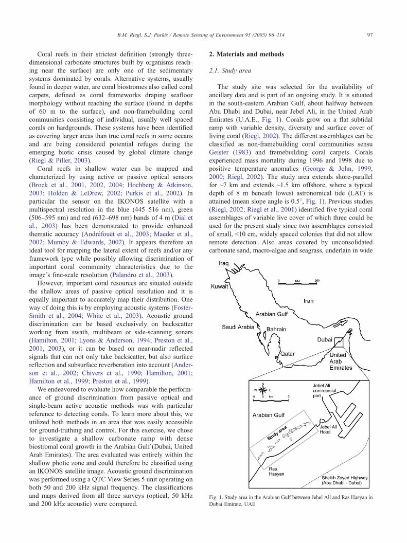
Fig. 1. Study area in the Arabian Gulf between Jebel Ali and Ras Hasyan in

Dubai Emirate, UAE.

B.M. Riegl, S.J. Purkis / Remote Sensing of Environment 95 (2005) 96–114 97

Coral reefs in their strictest definition (strongly three-

dimensional carbonate structures built by organisms reach-

ing near the surface) are only one of the sedimentary

systems dominated by corals. Alternative systems, usually

found in deeper water, are coral biostromes also called coral

carpets, defined as coral frameworks draping seafloor

morphology without reaching the surface (found in depths

of 60 m to the surface), and non-framebuilding coral

communities consisting of individual, usually well spaced

corals on hardgrounds. These systems have been identified

as covering larger areas than true coral reefs in some oceans

and are being considered potential refuges during the

emerging biotic crisis caused by global climate change

(Riegl & Piller, 2003).

Coral reefs in shallow water can be mapped and

characterized by using active or passive optical sensors

(Brock et al., 2001, 2002, 2004; Hochberg & Atkinson,

2003; Holden & LeDrew, 2002; Purkis et al., 2002). In

particular the sensor on the IKONOS satellite with a

multispectral resolution in the blue (445–516 nm), green

(506–595 nm) and red (632–698 nm) bands of 4 m (Dial et

al., 2003) has been demonstrated to provide enhanced

thematic accuracy (Andrefouet et al., 2003; Maeder et al.,

2002; Mumby & Edwards, 2002). It appears therefore an

ideal tool for mapping the lateral extent of reefs and/or any

framework type while possibly allowing discrimination of

important coral community characteristics due to the

image’s fine-scale resolution (Palandro et al., 2003).

However, important coral resources are situated outside

the shallow areas of passive optical resolution and it is

equally important to accurately map their distribution. One

way of doing this is by employing acoustic systems (Foster-

Smith et al., 2004; White et al., 2003). Acoustic ground

discrimination can be based exclusively on backscatter

working from swath, multibeam or side-scanning sonars

(Hamilton, 2001; Lyons & Anderson, 1994; Preston et al.,

2001, 2003), or it can be based on near-nadir reflected

signals that can not only take backscatter, but also surface

reflection and subsurface reverberation into account (Ander-

son et al., 2002; Chivers et al., 1990; Hamilton, 2001;

Hamilton et al., 1999; Preston et al., 1999).

We endeavored to evaluate how comparable the perform-

ance of ground discrimination from passive optical and

single-beam active acoustic methods was with particular

reference to detecting corals. To learn more about this, we

utilized both methods in an area that was easily accessible

for ground-truthing and control. For this exercise, we chose

to investigate a shallow carbonate ramp with dense

biostromal coral growth in the Arabian Gulf (Dubai, United

Arab Emirates). The area evaluated was entirely within the

shallow photic zone and could therefore be classified using

an IKONOS satellite image. Acoustic ground discrimination

was performed using a QTC View Series 5 unit operating on

both 50 and 200 kHz signal frequency. The classifications

and maps derived from all three surveys (optical, 50 kHz

and 200 kHz acoustic) were compared.

2. Materials and methods

2.1. Study area

The study site was selected for the availability of

ancillary data and is part of an ongoing study. It is situated

in the south-eastern Arabian Gulf, about halfway between

Abu Dhabi and Dubai, near Jebel Ali, in the United Arab

Emirates (U.A.E., Fig. 1). Corals grow on a flat subtidal

ramp with variable density, diversity and surface cover of

living coral (Riegl, 2002). The different assemblages can be

classified as non-framebuilding coral communities sensu

Geister (1983) and framebuilding coral carpets. Corals

experienced mass mortality during 1996 and 1998 due to

positive temperature anomalies (George & John, 1999,

2000; Riegl, 2002). The study area extends shore-parallel

for ~7 km and extends ~1.5 km offshore, where a typical

depth of 8 m beneath lowest astronomical tide (LAT) is

attained (mean slope angle is 0.58, Fig. 1). Previous studies(Riegl, 2002; Riegl et al., 2001) identified five typical coral

assemblages of variable live cover of which three could be

used for the present study since two assemblages consisted

of small, b10 cm, widely spaced colonies that did not allow

remote detection. Also areas covered by unconsolidated

carbonate sand, macro-algae and seagrass, underlain in wide

B.M. Riegl, S.J. Purkis / Remote Sensing of Environment 95 (2005) 96–11498

areas by early diagenetically cemented calcarenites (Evans

et al., 1973; Shinn, 1969), in this paper referred to as

hardground, were identified. Thus, for the sake of this study,

we could test whether the optical sensor would allow us to

spectrally discriminate corals from other, potentially spec-

trally similar benthos like algae. And we could test whether

the acoustic sensor was capable of detecting corals, which

we could define in this study area as areas of rugose

hardground as opposed to areas of flat hardground, not

settled by corals. Rubble areas, as alternative rugose

hardground areas, coincided with, and were derived from,

coral growth and therefore needed not to be separated.

2.2. The optical dataset

The image-base underlying our research consisted of an

IKONOS-2 11-bit multispectral satellite image of 4-m pixel

resolution in the red, green and blue bands and 1-m

resolution in the panchromatic band. For the present work,

only the red, green and blue bands were used due to the low

level returns from subsurface features with the panchromatic

band, which was deemed not useful for work underneath the

ocean surface. The image was acquired on 02 May 2001

(scene 75209) at 06:49 UTC. Sun elevation and nominal

collection azimuth at the time of acquisition were 678 and

658 respectively, the tidal stage was 3 h after high-water (0.9m above LAT), water clarity was high and the surface was

calm. The image was unaffected by atmospheric dust and

there was no cloud cover.

2.3. Optical ground-truthing

The optical techniques employed in this paper are adapted

and improved from previous work in the Red Sea by Purkis

and Pasterkamp (2004) and described in detail by Purkis

(2004, in press) and therefore only briefly revisited here.

Optical measurements were collected between 5th October

and 10th November 2002 using a suite of optical tools, used

concurrently to parameterize the reflectance of the dominant

reef substrata, both above and beneath the water surface and

the apparent optical properties of the water column. All

optical measurements were conducted over suitably large and

spatially homogeneous patches of substrate, between 10:00

and 17:45 h local time, therefore ensuring that the sun was a

minimum of 308 above the horizon, to preclude the effects ofdirectional illumination. Measurements were conducted from

the survey vessel and the location constrained with dGPS. To

obtain a measurement approximating to substrate reflectance

(Rb), an OceanOptics SD2000 fibre-optic spectrometer was

used beneath the water surface, at an elevation of 10 cm from

the target substrate (e.g. Hochberg&Atkinson, 2003; Holden

& LeDrew, 2002). The spectrometer was operated from the

vessel and twin 10-m fibre-optic cables were used to transmit

simultaneously acquired measurements of substrate radiance

and downwelling irradiance from the two submerged sensor

heads. Cross-calibration between the radiance and irradiance

channels of the instrument was conducted according to

Fargion and Mueller (2000) with use of a standard near-

lambertian reflectance panel and reflectance was calculated

according to Purkis and Pasterkamp (2004). Nearly coinci-

dent to the beneath water measurement, a PhotoResearch

PR650 spectroradiometer was used to evaluate remote-

sensing reflectance just above the water/air boundary (Rrs

(z=a) where z is depth, and a is air; standard notion for

measurements made above the water surface) of the

submerged substrate, sighted through the dcamera-styleT lensof the instrument. The measurement protocols of Pasterkamp

et al. (2003) were adhered to, and a near-concurrent sky

radiance measurement was used to correct for the effect of

sky radiance reflected at the water surface. Immediately prior

to, and following the substrate measurements, atmospheric

aerosol optical thickness at 550 nm (AOT550), was measured

using a hand-held Microtops II Sunphotometer and the

attenuation of the water body (k), was evaluated using a hand-

deployed PRR-600 Profiling Reflectance Radiometer system

(Biospherical Instruments) between 400 and 700 nm. In

accordance with the protocols of Mueller (2003), a PRR-610

Reference Radiometer, equipped with a cosine-corrector to

simultaneously measure downwelling irradiance in air, was

used to normalize the downwelling irradiance data acquired

beneath the surface.

2.4. Image acquisition and processing

To improve upon the already reasonable level of geo-

graphic accuracy for the IKONOS data, further geocorrection

was conducted against 40 ground control points acquired

using a portable Leica 500 real time kinematically (rtk)

corrected dGPS system with a horizontal accuracy of F30

cm, yielding an average root mean square (RMS) error of

0.66 pixel or 2.65 m. Prior to quantitative analysis, the

radiometric calibration coefficients of Peterson (2001) were

applied to convert pixel values from digital number to at-

sensor radiance units. Lacking in situ estimates of atmos-

pheric status at the time of image acquisition, we adopted the

empirical line method (Karpouzli & Malthus, 2003; Schott,

Salvaggio, & Volchok, 1988; Smith & Milton, 1999) for the

removal of atmospheric path radiance. In situ measurements

of surface reflectance were made over suitably large and

spatially uniform light and dark terrestrial pseudo-invariant

features (PIFs) (i.e. spectrally and radiometrically stable),

using the PR650. We selected a large homogeneous area of

desert sand and a large asphalt car park, the positions of which

were constrained using dGPS measurements, which were

subsequently located on the imagery. The literature shows

that both asphalt (Emery, Milton, & Felstead, 1998; Lawless,

Milton, & Anger, 1998; Schott et al., 1988) and desert sand

(Cosnefroy, Leroy, & Briottet, 1996; Lenny, Woodcock,

Collins, & Hamdi, 1996; Miesch, Cabot, Briottet, & Henry,

2003) are spectrally stable over long time periods and in

addition, are commonly used as vicarious (inflight) calibra-

tion targets for satellites. Against the PIFs, the imagery was


subsequently converted to apparent surface reflectance

using linear interpolation. The first 3 bands (blue (445–

516 nm), green (506–595 nm) and red (632–698 nm)) of

the imagery were further corrected for the influence of the

water column, to retrieve values equivalent to substrate

reflectance (Rb). The correction was implemented using the

optical equation described by Purkis and Pasterkamp

(2004) (Eq. (6)), where the bathymetric DEM (produced

by acoustic survey, see later sections) was used to provide

a depth (z) value on a pixel by pixel basis and the apparent

optical properties of the water column (Rw and k) were

derived from in situ measurements. The fact that optical

field campaign and imagery were not acquired simulta-

neously has implications for the values of k and Rw,

which, being apparent optical properties, vary with space

and time and therefore precludes the direct implementation

of the optical equation, as for Purkis and Pasterkamp

(2004). For this study the imagery and in situ optics were

related over a deep water reflectance target, the position of

which was constrained with dGPS. The target was visited

daily throughout the optics campaign at local times

appropriate to ensure comparable solar geometry to that

of sensor overpass. In rapid succession, k and Rrs (z=a)

were evaluated using the PRR-600 profiler and PR650,

respectively. The data was used to construct a look-up-

table of Rrs (z=a) versus k for a number of sea conditions.

A match was subsequently sought between satellite and

PR650 values of Rrs (z=a), with the result that in situ data

acquired 29/10/02 provided a match with an absolute error

in reflectance of 0.10%, 0.16% and 0.13% for bands 1, 2

and 3, respectively. The associated k and Rw spectra,

evaluated directly following the PR650 measurement were

resampled to the bandwidths and sensitivity of the

IKONOS sensor and used as input to the optical equation.

Implicit to this approach is the assumption that: (1) the

interplay between absorption and scattering governing the

observed reflectance of the water column, is relatively

consistent; (2) the optical properties of the water column

are homogeneous over the study area. The lack of fluvial

input into the area and personal experience leads us to

believe that the initial assumption is reasonable. Observa-

tions made during this and previous campaigns in the area

reveal that the dominant cause of water turbidity is high

sediment loading, caused by the suspension of uncon-

solidated sand during storm events. This being the case,

suspended particulates are the dominant parameter influ-

encing both Rrs (z=a) and k. Both the in situ optical

measurements and image acquisition occurred during

extensive calm periods with a high degree of water clarity.

Additionally, the sun elevation for both in situ and satellite

acquisition was constant (F658), as was the observation

angle of the IKONOS and PR650 (F258 off nadir). It is

reasonable to assume that the excellent match between

PR650 and satellite evaluated reflectance (average devia-

tion for bands 1–3 is b0.15%), will be accompanied by a

robust match in k. Lastly, considering the limited size of

the study area and the fact that sediment plumes are clearly

absent in the imagery, it is not unreasonable to assume that

the optical properties of the water body were likely to be

relatively homogeneous at the time of image acquisition.

2.5. Classification and accuracy assessment

Image classification was conducted using the multi-

variate normal probability driven classifier described by

Purkis and Pasterkamp (2004). The classifier was trained

solely using the sub-surface in situ spectral measurements of

substrate reflectance, resampled to the bandwidths and

sensitivity of the IKONOS sensor. To remain comparable

to the previous work in the region, both on the ground

(Riegl, 2002) and spaceborne (Andrefouet et al., 2003), the

in situ spectra were assembled into 8 broad facies classes

(Table 1).

As with the previous studies, 8 classes were found to

adequately represent the substrate diversity of the area. In

addition, other studies using IKONOS in comparable

environments (Andrefouet et al., 2003; Capolsini et al.,

2003; Maeder et al., 2002; Mumby & Edwards, 2002),

indicate that 8 classes is a realistic level of discrimination to

be expected from the capability of the sensor. The

classification was implemented on the IKONOS imagery

after it had been corrected for the radiative transfer effects of

both the atmosphere and water column. In this way, the link

between the in situ optical measurements and IKONOS data

was made at the level of substrate reflectance (Rb). A

discussion concerning the advantages and rationale behind

this approach, as opposed to the more traditional use of

dfrom-imageT trained classifiers, is given by Purkis and

Pasterkamp (2004).

During the field campaign, extensive ground-truthing

was conducted using SCUBA for the purpose of providing

validation data against which classification accuracy could

be assessed. A transect technique similar to that used by

Purkis et al. (2002) was employed, but adapted for use in

deeper water. The transects were typically 160�8 m

(equivalent to 80 IKONOS pixels) and substrate was

mapped to metre-resolution. The transect data was supple-

mented by a large quantity of spot checks throughout the

study area. Details concerning the collection and processing

of the ground-truth data are given in Purkis (2004). The

accuracy of the classified image was assessed against 15

transects and 52 spot checks, which totalled 524 validation

points. Since the classifier was trained exclusively using in

situ optics, all of the ground truth data remained independ-

ent and therefore available for accuracy assessment, with the

result that sufficient validation points were available to

support a statistical analysis of classification error without

bias (e.g. Congalton, 1991). Post-classification smoothing is

a commonly employed technique to improve accuracy by

reducing noise in the classified imagery (Mumby &

Edwards, 2002). A median filter was selected to smooth

the classification result, since it simultaneously reduces

Table 1

Summary of the typical substrate assemblages encompassed within each of the eight facies classes

Bottom class Typical assemblage composition Comments

Dense live coral Porites lutea and columnar Porites harrisoni

intermingled with Favia spp. and Platygyra spp.

Dense colonies over hardground, commonly maintaining a

low-relief but in places forming non-framebuilding coral

carpets. Coverage 50–100%.

Dense dead coral Acropora clathrata and A. downingi Dense dead tabular colonies, frequently overtopping and

heavily overgrown with algal turf and coralline algae.

In places the tabular framework has disintegrated into

piles of branch rubble. Average size of intact colonies is

1 to 1.5 m and coverage is 80–100%.

Sparse coral Porites, Favia spp. and Siderastrea savignyana

with occasional small colonies of Acropora clathrata

Widely spaced patches of Faviid and Siderastrea colonies

on hardground with occasional large Porites boulder corals.

The Acropora were mostly dead at the time of image

acquisition. Coverage is generally 10–40%.

Seagrass Mainly Halodule uninervis with occasional H. ovalis Dense seagrass stands had generally found over sandy–silty

substrate and had a coverage of 60–80%.

Shallow algae Rhizoclonium tortuosum, Chaetomorpha gracilis

and Cladophora coelothrix

Extensive mats over sandy–silty substrates, often associated

with seagrasses. Coverage 80–100%.

Deep algae Sargassum binderi, S. decurrens,

Avrainvillea amedelpha and Padina

Moderately dense stands of macro-algae on patches of

unconsolidated sediment. Coverage 30–60%.

Hardground – Large slabs of lithified carbonate sediment, fringed by

dtepeeT structures. Coverage 100%.

Sand – Unconsolidated carbonate sand. Coverage 100%.

Coverage refers to the percentage of the seabed occupied when a 1�1 m area of substrate is viewed from nadir at an altitude of 1 m. Assemblage description is

based on Riegl (2002).


noise while preserving patch edges characteristics. Code

written in Matlab 6.1 was used to implement a median filter

constructed using a 3�3 pixel neighborhood.

2.6. The acoustic dataset

The acoustic survey was conducted from a 15-m survey

vessel equipped with a real-time kinematic (rtk) differ-

entially corrected Fugro SeaSTAR 3200LR12 global

positioning system (dGPS). The differential correction of

the positioning data was conducted in real-time against the

Omnistar network of satellites with a horizontal accuracy

of F50 cm. The geo-rectified satellite image was loaded

into the softwares Fugawi and Hypack, which were

interfaced with the dGPS unit and allowed the operator

monitoring vessel position with respect to the imagery in

real-time. To ensure an adequate degree of accuracy, three

independent acoustic surveys were used to build the

bathymetric DEM for interface with optical remote-sens-

ing. Bathymetry lines were obtained over the entire study

area using both a 50 and 200 kHz signal with 0.4-ms pulse

width and a 5-Hz sampling frequency with a beam angle

of 428 and 128, respectively, for the two sampling

frequencies provided by a Suzuki 5200 depth sounder

with a minimum depth of operation of 1 m. Surveys were

executed in sequence (first 50, then 200 kHz) over a

period of 5 days. The same planned line files were used

for navigation in order to ensure closest possible spatial

coincidence of data in the two surveys. The 50 kHz survey

covered a wider overall area than the 200 kHz survey, but

for this study only lines coincident in both surveys were

used. Depth was determined by using the QTC View5

bottom picking algorithm, which was accurate to 10 cm.

Accuracy of the algorithm was tested with bar checks

(Brinker & Minnick, 1994) and by direct cross-checks of

displayed bathymetry and measured depth with a weighted

line at several sites. Survey lines were spaced by 100 m to

cover the entire study area (7�1.5 km). An additional 50

kHz acoustic near-shore bathymetry survey with a 15-m

line spacing provided high-resolution bathymetry in the

first 500 m from shore, these data were only used in

optical algorithms but not for acoustic ground discrim-

ination. Throughout the survey period, tidal data was

collected at five-minute intervals in situ, using a sub-

merged Van Essen DI-240 pressure logger. A duplicate

logger was used to record atmospheric pressure above the

water surface and therefore remove any influence from

atmospheric variation. Tidally corrected 50 kHz data were

used to construct a DEM referenced to lowest astronomical

tide (LAT). The merged bathymetry data was interpolated

to a regular grid of equal size to the pixel elements of the

IKONOS image (4�4 m) using triangle-based linear

interpolation implemented using Code written in Matlab

6.1, yielding a single depth value per satellite pixel. The

accuracy of the resulting DEM was assessed against the

200 kHz survey lines and error was found to be less than

0.05 m.

Acoustic habitat classification was performed using the

QTC View Series 5 system which consists of hydrographic

survey hard- and software geared towards acoustic ground

discrimination based on the shape of sonar returns (Quester

Tangent, 2002). It records the characteristics of reflected

waveforms to generate habitat classifications based on the

diversity of scattering and penetration properties of different


types of seafloor (Preston et al., 1999). The typical process

involves a hydrographic survey where raw acoustic data are

collected as time-stamped, dGPS-geolocated, digitized

envelopes of the first echo. Data were processed in the

software QTC Impact and were checked by the operator for

correct time-stamps, correct depths and correct signal

strengths. All signals that did not pass an appropriate level

of quality control were discarded. Data were displayed on a

bathymetry plot, where recorded depths were checked

against the blanking (minimum recordable) and maximum

depths set for the survey and any faulty depth picks were

removed manually before further processing.

In QTC Impact software, the echoes were digitized,

subjected to Fourier Analysis, Wavelet analysis and were

analysed for kurtosis, area under the curve, spectral

moments and other variables by the acquisition software

(Legendre et al., 2002). After being normalized to a range

between 0 and unity, they were subjected to Principal

Components Analysis (PCA) in order to eliminate redun-

dancies and noise. The first three principal components of

each echo were retained (called Q values), according to the

logic that these typically contain 95% of the information

(Quester Tangent, 2002). Datapoints were then projected

into pseudo-three-dimensional space along these three

components, where they were then subjected to cluster

analysis (Quester Tangent, 2002).

2.7. Acoustic classification and accuracy assessment

Cluster analysis using a Bayesian approach was per-

formed within the software package QTC Impact, which is

companion software to the QTC View survey package. In

clustering, the user decides on the number of desirable

clusters and also chooses which cluster to split and how

often. Clustering decisions are guided by three statistics that

are offered by the program called bCPIQ (Cluster Perform-

ance Index), bChi2Q and bTotal ScoreQ. Total score decreasesto an inflection point which is da strong indication of best

split levelT (Quester Tangent, 2002). CPI increases with

increased cluster split, while Chi2 decreases, reaching

maximum/minimum values at optimal split level (Quester

Tangent, 2002). We plotted Total Score against the number

of clusters to investigate ideal cluster split. However, we

always split acoustic data until as many acoustic classes

were obtained as optical classes could be distinguished on

the IKONOS image. This was done because we wanted to

evaluate whether both methods allowed comparable dis-

crimination accuracy.

Reviews of the functioning of the QTC system and

critiques can be found in Hamilton et al. (1999), Hamilton

(2001), Legendre et al. (2002), Preston and Kirlin (2002)

and Legendre (2002).

For each individual signal, the following data were

exported from QTC Impact for further processing: latitude,

longitude, depth (uncorrected for tidal state, correction was

performed during data re-processing), the first three PCA

axes (called Q-axes), a class category, a class assignment

confidence value and a class probability value both ranging

from 0 to 100%. Class confidence is da measure of the

covariance-weighted distances between the position of the

record and the positions of all cluster centersT while class

probability is da measure of closeness to the cluster center,

weighted by the covariance of the cluster in the direction of

the recordT (Quester Tangent, 2002). These indices are

useful for the detection of class boundaries (Morrison et al.,

2001) and we used them to evaluate the overall bqualityQ ofindividual data-points and classes following the rationale

that anything with predominantly low confidence and/or

probability could be good candidates for deletion from the

dataset. We used these statistics to create several levels of

datasets that were tested against each other: one level with

all data and all classes included, and several levels in which

all data that did not fulfil specified quality control criteria

(i.e. b90%, 60% confidence, b90%, 60% probability) and

all classes that did not show clear spatial patterns, were

culled. The discrimination accuracies of the datasets were

then compared against each other. Datasets were reduced to

three-column matrices consisting of a single x,y geo-

referenced class category z. The trackplots for each data

class were individually plotted to allow assessment of their

spatial distribution. Classes that showed a preferential

distribution in well-defined parts of the survey area were

considered to show promise for distinguishing different

seafloor types. Classes that were found in comparable

density across the entire survey area were considered to

carry signals with no discrimination ability. Classes that

were found to be redundant were iteratively removed from

the dataset.

Finally, we resampled the irregular grid of categorical

data consisting of the georeferenced class categories

obtained from the cluster analysis to a regular grid and

used a nearest neighbour interpolation to fill the grid and

then to obtain a filled contourplot of class distribution

(Middleton, 2000). The nearest neighbor algorithm was

used to not produce fractions of classes such as would be

produced by, for example, kriging, which, in the present

case of categorical variables on a nominal scale, would have

been non-sensical.

Groundtruthing used a total of 75 points to determine

accuracy of the maps derived from 50 and 200 kHz surveys

(Fig. 8). The correspondence of the acoustic and the optic

dataset was estimated by using 97 gridded points that were

projected onto the overlaid maps (Fig. 8).

3. Results

3.1. Optical results

The results of the optical classification allowed the

mapping of the previously assigned eight classes (Fig. 2).

Classes were split into unconsolidated sediments (shallow

Fig. 2. Classification of IKONOS satellite image of the survey area. The headland to the left is Ras Hasyan, Jebel Ali is just outside the right picture border.

Pixel size is 4�4 m. See Table 1 for further details.


sand) and the associated bottom-types (seagrass, shallow

algae) in nearshore areas, and hardgrounds, sparse coral,

dense coral and some sand in the deeper areas.

Accuracy assessment of the predictive map yielded an

overall accuracy of 69% and a Tau coefficient (Ma &

Redmond, 1995) of 65% (Table 2). It should be noted that

the accuracy assessment is likely to be pessimistically

biased since the transect positions were selected to span

heterogeneous areas of seafloor in an effort to capture and

quantify classification errors at patch boundaries. Therefore

the accuracy of 69% can be considered a true worst-case

Table 2

Error matrix calculated for the classified imagery

Row to

tals

Sand

Swallow algae

Deep algae

Seagrass

Hardground

Dense dead coral

Dense live coral

Sparse coral

Sand

Swallow

alga

e

Deep a

lgae

Seagr

ass

Hardgr

ound

Dense

dead

coral

Dense

live

coral

Sparse

coral

4 2 12 0 0 5 1 6

4 37 3 0 0

0

0

0

11 0 12

6 5

0 0

0 0

71 1 4 7 7

0 17 2 0

0

2

0 11 91 6

4 4 0 0 026 2

0 1 3 3 10 73 18

0

1

1

1 0 0 5 0 3 42

30

67

101

21

108

37

109

51

52418 47 91 32 101 56 86 93

Ground-truth data

Cla

ssif

ied

data

Column totals

PO=69% (95% confidence intervals of PO are 73% to 65%) T=65% (95% confidence intervals of T are 69% to 61%)

The ground-truth pixels that are classified as the correct substrate classes

are located along the major diagonal of the matrix, while all non-diagonal

elements represent errors of omission or commission. T=Tau index.

69%. If accuracy is assessed against only the spot check

points, which were collected without any a priori knowledge

of substrate distribution and therefore more likely to fall

within homogeneous patches, an accuracy of 81% is

achieved (Tau=77%).

3.2. Acoustic results

The 50 kHz data, when plotted along the first three

principal components after signal processing, formed a

relatively homogeneous cluster, indicating that overlap

between data classes could be expected (Fig. 3). Since the

number of splits performed in the employed version of

QTC Impact software is user-defined, we iteratively

increased the number of splits from two clusters to eight

clusters, the highest number of bottom classes derived

from the optical image classification. Since the data cloud

was more or less spherical, clusters were split first along

the PC1 (Q1) axis and then along the PC2 (Q2) axis.

Splitting along the PC2 axis resulted in a pattern of

parallel, relatively discrete, clusters and was preferred over

the clusters obtained by splitting along the PC1 axis,

which showed more overlap and less clear separation. The

Total Score statistic showed the strongest drop after the

first split both for PC1 and PC2 splits. The splits along the

PC1 axis showed an inflexion point after five splits, along

the PC2 axis after 6 splits (Fig. 3), which indicated that

this would be the optimal number of classes. We never-

theless proceeded to obtain 8 clusters, for comparability

reasons with the optical dataset. Of these, classes 6 and 8

had the highest probability scores. However, class 6 had

low confidence scores, while those of class 8 were high

(Fig. 3C and D). Probability scores were more uniformly

distributed among classes than confidence scores. In

general, the distribution of the probability statistic was

Fig. 3. Clustering statistics for the 50 kHz survey. (A) PCA plot. Only 1% of data is shown for reasons of graphic clarity. Data belonging to different clusters are

coded by different symbols. (B) The inflection point of the Total Score statistic shows the presumed ideal number of clusters. In the present case it is 6 clusters.

(C) The Confidence statistic describes the probability that a record indeed belongs to the group it is assigned to by the analysis. (D) The Probability statistic is a

measure of the records’ closeness to the center of their assigned cluster. The low values indicate the wide spread of data in the relatively homogeneous cloud.


clearly skewed towards lower values in all classes, while

confidence was markedly skewed towards high values.

Fig. 4A shows the first three principal components of the

processed 200 kHz data. The data cloud was less compact

than that of the 50 kHz signals and shows better separation,

although also in this case no distinct clusters are visible. All

clusters were consecutively split along their PC1 axis, which

resulted in parallel groups. In this case, a split along the PC2

Fig. 4. Clustering statistics for the 200 kHz survey. (A) PCA plot. Only 2% of data is shown for reasons of graphic clarity. Symbols code data clusters. (B) The

inflection point of the Total Score statistic shows that the ideal number of clusters would be 3. (C) Confidence statistic. (D) Probability statistic as in Fig. 3.


axis was not performed, since the datacloud was markedly

oblong along the PC1 axis and therefore suggested one

natural direction of cluster separation. Total score, as a

measure of ideal clustering level, showed three inflexion

points, one each after three, five and seven splits (Fig. 4B).

The strongest inflexion occurred after three clusters,

suggesting that this might be the ideal number of clusters.

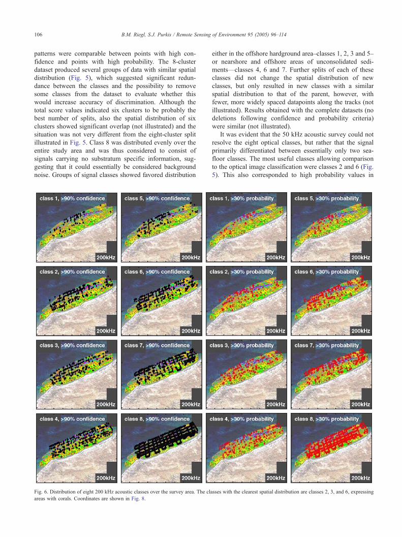
This assumption was later confirmed, three classes (2, 3 and

7) had a well-defined spatial pattern (Fig. 6). However, data

were also in this case split to an eight-cluster level to check

for comparability with the optical dataset. Class 1 had the

highest observed confidence values (Fig. 4C). Probability

values were similar between the classes and no clear trend

was evident (Fig. 4). Also in the 200 kHz dataset,


probability scores were more uniform than confidence

scores among classes. In general, the distribution of

probabilities was clearly skewed towards lower values in

all classes, while confidence classes were markedly skewed

towards high values.

Since the PC2 axis splits produced the better cluster

separation in the 50 kHz survey, we used these data to plot

the trackplots of each class in order to understand their

spatial pattern. In the 200 kHz survey, we used the splits

obtained along the PC1 axis. Two sets of trackplots were

made for each survey: one with all data, and one with data

only exceeding certain confidence and probability values

that were then superimposed over the classified IKONOS

image. Three levels of confidence (N80%, 90%, 95%) and

probability (30%, 50%, 60%) were tested and data were

repeatedly plotted. Useful levels were 90% confidence and

Fig. 5. Distribution of eight 50 kHz acoustic classes over the survey area. Th

hardgrounds, and 6, expressing unconsolidated sediments. Coordinates are shown

30% probability for both frequencies. These manipulations

eliminated 26.2% of 50 kHz data and 37.8% of 200 kHz

data when the confidence criterium was applied, but 55.4%

of 50 kHz data and 52.8% of 200 kHz data when the

probability criterium was applied. When probabilities N50%

were required, entire classes could no longer be evaluated

for any coherent spatial patterns in both frequencies. Also,

when accuracies N95% were demanded, overall less than

half of the datapoints remained. This, besides the tight

packing of clusters in Figs. 3 and 4, we considered another

indication for the relatively homogeneous nature of the

dataset with poor definition of individual clusters.

Fig. 5 shows the distribution of eight 50 kHz acoustic

classes along the survey lines. The lines obtained with

N90% confidence data were similar to those of the full

dataset since about two thirds of data was retained. Spatial

e classes with the clearest spatial distribution are classes 2, expressing

in Fig. 9.


patterns were comparable between points with high con-

fidence and points with high probability. The 8-cluster

dataset produced several groups of data with similar spatial

distribution (Fig. 5), which suggested significant redun-

dance between the classes and the possibility to remove

some classes from the dataset to evaluate whether this

would increase accuracy of discrimination. Although the

total score values indicated six clusters to be probably the

best number of splits, also the spatial distribution of six

clusters showed significant overlap (not illustrated) and the

situation was not very different from the eight-cluster split

illustrated in Fig. 5. Class 8 was distributed evenly over the

entire study area and was thus considered to consist of

signals carrying no substratum specific information, sug-

gesting that it could essentially be considered background

noise. Groups of signal classes showed favored distribution

Fig. 6. Distribution of eight 200 kHz acoustic classes over the survey area. The cl

areas with corals. Coordinates are shown in Fig. 8.

either in the offshore hardground area–classes 1, 2, 3 and 5–

or nearshore and offshore areas of unconsolidated sedi-

ments—classes 4, 6 and 7. Further splits of each of these

classes did not change the spatial distribution of new

classes, but only resulted in new classes with a similar

spatial distribution to that of the parent, however, with

fewer, more widely spaced datapoints along the tracks (not

illustrated). Results obtained with the complete datasets (no

deletions following confidence and probability criteria)

were similar (not illustrated).

It was evident that the 50 kHz acoustic survey could not

resolve the eight optical classes, but rather that the signal

primarily differentiated between essentially only two sea-

floor classes. The most useful classes allowing comparison

to the optical image classification were classes 2 and 6 (Fig.

5). This also corresponded to high probability values in

asses with the clearest spatial distribution are classes 2, 3, and 6, expressing


these two classes (Fig. 3C and D). However, class 6 had low

confidence values. The uniformity of probability values

across all eight classes would not have made this choice

obvious from the beginning (Fig. 3). Also confidence values

would not have allowed us to predict immediately after the

cluster analysis and before the visualization of the trackplots

which classes were likely to have the clearest and easiest-to-

interpret spatial distribution. While other data classes also

had a distinct spatial distribution, such as classes 3 and 7

(offshore), the data in these classes were too sparse to be

useful.

In order to be able to better interpret the spatial patterns

of the classes, we resampled the data to a regular grid and

used a nearest neighbor interpolation to obtain filled

contourplots of the distribution of the class variables. We

attempted to produce four different maps—firstly with all

data in classes 2 and 6, secondly with only those data with

N90% confidence and N 30% probability in classes 2 and 6,

thirdly with all data in all classes and finally with all classes

but only those data with N90% confidence and N30%

probability. Of these four surfaces, only those produced

uniquely with data in classes 2 and 6 were successful

(Fig.7). The high density of the classes with no spatial

preference (in particular class 8) led to no useable gridding

and interpolation results when all classes were plotted (not

illustrated). Accuracy was poor overall. In particular in the

offshore area, significant confusion between visually iden-

tified sand and optically identified hardgrounds existed.

However, much of the offshore sand is only a few

centimeter-thick sheet overlying hardgrounds, resulting in

a visual (optical) sand signature but an acoustic hardground

signature.

Also the distribution of the N90% confidence and

N30% probability 200 kHz data in each of the eight

classes was plotted along the survey lines (Fig. 6).

Classes 1, 2, 3, 5 and 7 showed clear spatial patterns,

but classes 1 and 5 contained few data and coincided in

distribution with the other classes, therefore, they were

not considered useful. When all data (no deletion of

points b90% confidence and/or 30% probability) were

used, the spatial patterns were less apparent. Class 8 was

almost ubiquitous and was therefore considered to carry

little information.

In both evaluations (full dataset and N90% confidence,

N30% probability only), classes 1, 2, and 3 showed a clearly

preferential distribution in the offshore area where most

coral growth was found, while classes 4 and 7 were

preferentially distributed in non-coral areas (Fig. 6). Four

different spatial prediction maps were produced by nearest

neighbor interpolation—firstly with all data in classes 2, 3

(both coded as class 1) versus 4 and 7 (both coded as class

2), secondly with only those data with N90% confidence and

N 30% probability in classes 2, 3 versus 4 and 7, thirdly with

all data in all classes and finally with all classes but only

those data with N90% confidence and N 30% probability.

The maps produced with all classes did not provide any

useful results, which is not surprising in view of the

ubiquitous class 8 (not illustrated).

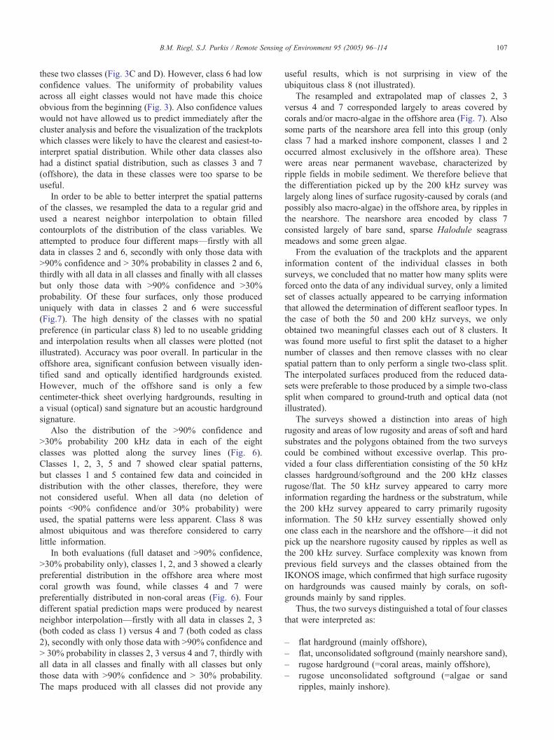
The resampled and extrapolated map of classes 2, 3

versus 4 and 7 corresponded largely to areas covered by

corals and/or macro-algae in the offshore area (Fig. 7). Also

some parts of the nearshore area fell into this group (only

class 7 had a marked inshore component, classes 1 and 2

occurred almost exclusively in the offshore area). These

were areas near permanent wavebase, characterized by

ripple fields in mobile sediment. We therefore believe that

the differentiation picked up by the 200 kHz survey was

largely along lines of surface rugosity-caused by corals (and

possibly also macro-algae) in the offshore area, by ripples in

the nearshore. The nearshore area encoded by class 7

consisted largely of bare sand, sparse Halodule seagrass

meadows and some green algae.

From the evaluation of the trackplots and the apparent

information content of the individual classes in both

surveys, we concluded that no matter how many splits were

forced onto the data of any individual survey, only a limited

set of classes actually appeared to be carrying information

that allowed the determination of different seafloor types. In

the case of both the 50 and 200 kHz surveys, we only

obtained two meaningful classes each out of 8 clusters. It

was found more useful to first split the dataset to a higher

number of classes and then remove classes with no clear

spatial pattern than to only perform a single two-class split.

The interpolated surfaces produced from the reduced data-

sets were preferable to those produced by a simple two-class

split when compared to ground-truth and optical data (not

illustrated).

The surveys showed a distinction into areas of high

rugosity and areas of low rugosity and areas of soft and hard

substrates and the polygons obtained from the two surveys

could be combined without excessive overlap. This pro-

vided a four class differentiation consisting of the 50 kHz

classes hardground/softground and the 200 kHz classes

rugose/flat. The 50 kHz survey appeared to carry more

information regarding the hardness or the substratum, while

the 200 kHz survey appeared to carry primarily rugosity

information. The 50 kHz survey essentially showed only

one class each in the nearshore and the offshore—it did not

pick up the nearshore rugosity caused by ripples as well as

the 200 kHz survey. Surface complexity was known from

previous field surveys and the classes obtained from the

IKONOS image, which confirmed that high surface rugosity

on hardgrounds was caused mainly by corals, on soft-

grounds mainly by sand ripples.

Thus, the two surveys distinguished a total of four classes

that were interpreted as:

– flat hardground (mainly offshore),

– flat, unconsolidated softground (mainly nearshore sand),

– rugose hardground (=coral areas, mainly offshore),

– rugose unconsolidated softground (=algae or sand

ripples, mainly inshore).

Fig. 7. Contours of the extrapolated two-class models obtained after data processing. The 50 kHz maps show hardground areas in red, softground in yellow.

The 200 kHz maps show rugose areas in red, flat areas in yellow. The polygons from the maps were combined (50 kHz plus 200 kHz for each type of data

processing) to produce the maps in Fig. 8. White dots represent ground-truthing points in coral areas, black dots represent ground-truthing points in non-coral

areas. Coordinates are in UTM, Zone 40R north, WGS 1984, coordinates are the same in all four figures.


Each survey distinguished two classes: the 200 kHz survey

distinguished between rugose and flat areas of seafloor and

was thus found more useful for detecting corals. The 50 kHz

survey distinguished primarily between hard and soft

substrates and was found to be sensitive to subsurface

texture (i.e. hardgrounds underlying unconsolidated sand

sheets) and was in the present case not useful for the

detection of corals.

In the next step, the polygons obtained from the 50

and 200 kHz surveys were combined into single, four-

class maps. Two such four class maps were produced

(Fig. 8): one which used all data in clusters 2 and 8 (50

kHz) and 2, 3 versus 4, 7 (200 kHz), and one which used

only the data N90% confidence and N30% probability.

Both were superimposed on the classified IKONOS

imagery and error matrices were calculated (Tables 3 and

4). The map produced from the more intensely processed

data (N90% confidence and N30% probability) was more

accurate than the map incorporating all data (66%, T=59

versus 60%, T=53). This supports the importance of

significant data-processing. The accuracy of the more

intensely processed map against ground-truthing points

was 56% (T=46) (Table 5).

Seagrass, which in the study area consisted only of

very sparse Halodule uninervis and Halophila ovalis,

was not observed to provide any acoustic signature. This

was verified by obtaining short sample datasets over

seagrass and nearby bare sand. The acoustic data, when

treated in the same way as described above, did not split

into any interpretable clusters. The three different classes

of coral communities that were discriminated by the

IKONOS classification were not at all resolved by the

acoustic survey, but corals were nevertheless distin-

guished acoustically with relatively high accuracies as

rugose hardground.

Finally, to evaluate whether the clusters were caused by

depth contamination of the signal, we plotted the relative

frequency of each of the eight classes obtained in both

surveys against depth (Fig. 9). Although some of the 50 kHz

classes showed depth preference, they occurred across much

of the survey area’s depth range and showed wide overlap.

If depth had influenced the signal, the substantial overlap in

the depth distribution of the classes should not have been

observed.

Also the 200 kHz classes did not show a clear depth

preference (Fig. 9). It was therefore concluded that depth

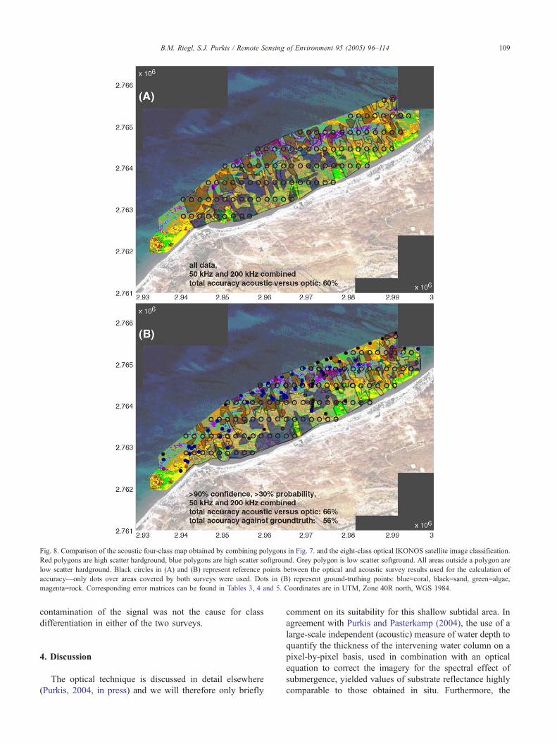
Fig. 8. Comparison of the acoustic four-class map obtained by combining polygons in Fig. 7. and the eight-class optical IKONOS satellite image classification.

Red polygons are high scatter hardground, blue polygons are high scatter softground. Grey polygon is low scatter softground. All areas outside a polygon are

low scatter hardground. Black circles in (A) and (B) represent reference points between the optical and acoustic survey results used for the calculation of

accuracy—only dots over areas covered by both surveys were used. Dots in (B) represent ground-truthing points: blue=coral, black=sand, green=algae,

magenta=rock. Corresponding error matrices can be found in Tables 3, 4 and 5. Coordinates are in UTM, Zone 40R north, WGS 1984.


contamination of the signal was not the cause for class

differentiation in either of the two surveys.

4. Discussion

The optical technique is discussed in detail elsewhere

(Purkis, 2004, in press) and we will therefore only briefly

comment on its suitability for this shallow subtidal area. In

agreement with Purkis and Pasterkamp (2004), the use of a

large-scale independent (acoustic) measure of water depth to

quantify the thickness of the intervening water column on a

pixel-by-pixel basis, used in combination with an optical

equation to correct the imagery for the spectral effect of

submergence, yielded values of substrate reflectance highly

comparable to those obtained in situ. Furthermore, the

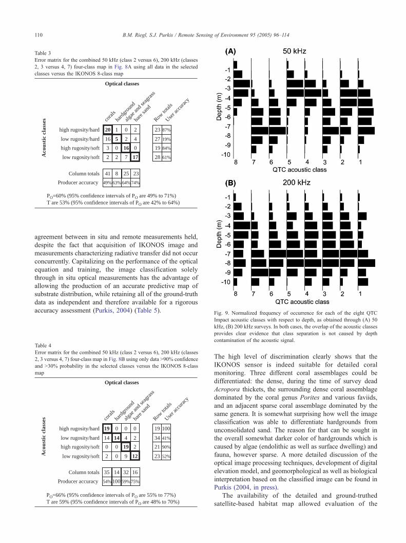
Table 3

Error matrix for the combined 50 kHz (class 2 versus 6), 200 kHz (classes

2, 3 versus 4, 7) four-class map in Fig. 8A using all data in the selected

classes versus the IKONOS 8-class map

20 1 0

16 5 2

3 0 16

23

27

19

41 8 25

Optical classes

Aco

usti

c cl

asse

s

49% 63% 64%

87%

19%

PO=60% (95% confidence intervals of PO are 49% to 71%) T are 53% (95% confidence intervals of PO are 42% to 64%)

172 72

0

4

2

28 61%

84%

23

74%

low rugosity/hard

high rugosity/hard

high rugosity/soft

Column totals

Producer accuracy

low rugosity/soft

Row to

tals

hard

grou

nd

coral

s

algae

and s

eagr

ass

User a

ccur

acy

bare

sand

Fig. 9. Normalized frequency of occurrence for each of the eight QTC


agreement between in situ and remote measurements held,

despite the fact that acquisition of IKONOS image and

measurements characterizing radiative transfer did not occur

concurrently. Capitalizing on the performance of the optical

equation and training, the image classification solely

through in situ optical measurements has the advantage of

allowing the production of an accurate predictive map of

substrate distribution, while retaining all of the ground-truth

data as independent and therefore available for a rigorous

accuracy assessment (Purkis, 2004) (Table 5).

able 4

rror matrix for the combined 50 kHz (class 2 versus 6), 200 kHz (classes

, 3 versus 4, 7) four-class map in Fig. 8B using only data N90% confidence

nd N30% probability in the selected classes versus the IKONOS 8-class

ap

Row to

tals

low rugosity/hard

high rugosity/hard

high rugosity/soft

hard

grou

nd

coral

s

algae

and s

eagr

ass

19 0 0

14 14 4

0 0 19

19

34

21

35 14 32

Optical classes

Aco

usti

c cl

asse

s

Column totals

Producer accuracy

User a

ccur

acy

54% 100 59%

100

41%

PO=66% (95% confidence intervals of PO are 55% to 77%)

122 90

2

2

0

23 52%

90%

16

75%

bare

sand

low rugosity/soft

Impact acoustic classes with respect to depth, as obtained through (A) 50

kHz, (B) 200 kHz surveys. In both cases, the overlap of the acoustic classes

provides clear evidence that class separation is not caused by depth

contamination of the acoustic signal.
T
E

2

a

m

T are 59% (95% confidence intervals of PO are 48% to 70%)

The high level of discrimination clearly shows that the

IKONOS sensor is indeed suitable for detailed coral

monitoring. Three different coral assemblages could be

differentiated: the dense, during the time of survey dead

Acropora thickets, the surrounding dense coral assemblage

dominated by the coral genus Porites and various faviids,

and an adjacent sparse coral assemblage dominated by the

same genera. It is somewhat surprising how well the image

classification was able to differentiate hardgrounds from

unconsolidated sand. The reason for that can be sought in

the overall somewhat darker color of hardgrounds which is

caused by algae (endolithic as well as surface dwelling) and

fauna, however sparse. A more detailed discussion of the

optical image processing techniques, development of digital

elevation model, and geomorphological as well as biological

interpretation based on the classified image can be found in

Purkis (2004, in press).

The availability of the detailed and ground-truthed

satellite-based habitat map allowed evaluation of the

Table 5

Error matrix for the combined 50 kHz (class 2 versus 6), 200 kHz (classes

2, 3 versus 4, 7) four-class map in Fig. 8B using only data N90% confidence

and N30% probability in the selected classes versus ground-truthing points

19 10 2

10 2 3

0 0 5

35

16

6

29 12 12

Grountruthed classes

Aco

usti

c cl

asse

s

66% 17% 42%

54%

13%

PO=56% (95% confidence intervals of PO are 42% to 70%) T are 46% (95% confidence intervals of PO are 32% to 60%)

160 20

1

1

4

18 89%

83%

22

73%

low rugosity/hard

high rugosity/hard

high rugosity/soft

Column totals

Producer accuracy

low rugosity/soft

Row to

tals

hard

grou

nd

coral

s

algae

and s

eagr

ass

User a

ccur

acy

bare

sand


information content within the acoustic QTC View classes

obtained during our surveys. The analysis of the present

dataset showed how the statistics provided by the QTC

Impact software can be used to refine results by

deleting datapoints and entire classes. This procedure

(deletion of datapoints with low confidence/probability,

deletion of classes without clearly visible spatial

patterns) increased the ease of interpretation as well as

accuracy in the case of our study. The finding that

increased levels of data processing also increases the

accuracy of the product concurs with the report by

Purkis and Pasterkamp (2004) for Landsat imagery. The

result is also important when considering the validity of

the QTC View as an operational tool in an area of

unknown bottom-type mosaic since the evaluation of

what classes and level of data processing should be the

final output may be difficult. Without having a known

habitat mosaic for comparison (in our case the IKONOS

image), it may not be evident how to select the best

classes from the provided statistics. Our presented

analyses here may be helpful to guide selection of

what data should be used and what should be discarded.

Also Morrison et al. (2001) found the probability and

confidence statistics useful in finding habitat boundaries

in soft sediments.

It was easily visible that of the eight acoustic classes

obtained from the supervised classification process not all

did carry useable information. More classes had a more or

less ubiquitous than spatially preferential distribution.

Acoustic signals show a lot of random variability, which

is caused by ship and sensor movement, hardware config-

uration, natural variability, electromagnetic interference,

random signal noise, etc. (Hamilton, 2001; Hamilton et

al., 1999). To obtain signal stability, a given number of

pings are stacked to produce an averaged signal which helps

to avoid fluctuations and the averaged signals thus make the

detection of patterns easier. In QTC View, while every

individual echo is collected and digitized, four consecutive

echoes are then stacked for averaging. Different ways of

stacking are recommended for different bottom types

(Hamilton, 2001; Hamilton et al., 1999) and different

systems stack different numbers of pings (Walter et al.,

2002). While stacking is necessary to compensate for

the semi-random nature of the returns and yet harness

their usability, it also has the effect of producing

averaged footprints. When the survey vessel moves,

the stacked footprint can include several bottom classes

and will increase in size with vessel speed. Since coral

reefs are notorious for their spatial heterogeneity, it is

not surprising that only relatively few pure stacked

echoes of any one substratum class were obtained, while

a majority of signals were in reality an average of

several bottom classes. We believe that this mechanism,

coupled with natural and survey-dependent (hardware,

weather, etc.) signal variability, helped create the data

classes that were distributed evenly over the survey

areas and did not distinguish any bottom types (Figs. 5

and 6).

The footprint of the 50 kHz transducer was much

bigger than that of the 200 kHz transducer. Consequently,

spatial resolution was higher and ecological grain finer in

the 200 kHz survey. This was important for distinguishing

ecologically relevant units, such as coral versus bare

hardground. Corals, the main target to be mapped, had

average diameters of less than 1 m in the study area,

which translates to 2 adjacent 200 kHz footprints, but only

one half 50 kHz footprint at 5 m depth, where the densest

coral assemblages are found (Riegl, 2002). It can be easily

seen that each individual 50 kHz footprint was bigger than

several fully-grown coral colonies (0.84–3.36 m2 footprint

size versus 0.8 m2 maximum expected coral size). When

adding the fact that four consecutive signals were stacked,

the footprint actually increased fourfold since survey speed

was such that individual footprints did not overlap. In our

survey, 50 kHz footprints had areas of 3.36 (at 5 m

depth)–13.44 m2 (at 10 m depth) at a speed of 10 km/h

and a ping rate of 5 Hz. Except in very dense coral areas,

such footprints were likely to include more bare sub-

stratum than coral. The 200 kHz footprint, in contrast

varied in the same depth range from 0.21 to 0.84 m2 pre-

stacked and 0.84 (at 5 m depth)–3.36 m2 (at 10 m depth).

This was sufficiently small to include enough bpure coralQfootprints to obtain acoustic classes determining corals.

Also, over rough terrain, such as corals, signal averaging

can indeed degrade the signals and lead to misclassifica-

tions (Hamilton, 2001; Hamilton et al., 1999) and

McKinney and Anderson (1964) found scattering to vary

widely over corals (Hamilton et al., 1999). It is therefore

not surprising that signal classes encoding corals were not

very well defined (classes 2, 3, and 7 of the 200 kHz


survey, Figs. 7 and 8). Hamilton (2001) and Hamilton et

al. (1999) suggest using the variability in the pings rather

than averaging in such areas.

It is also known that surface scatter from a statisti-

cally rough surface is inversely dependent on transducer

opening angle (Clay & Sandness, 1971; Medwin & Clay,

1998). The smaller-opening angle 200 kHz transducer

therefore not only had a smaller footprint allowing for

higher becologicalQ precision, but it also produced

relatively higher backscatter, which would suggest that

this makes it a good tool for detecting surface structures,

such as the scatter caused by corals, maroalgae, or sand

ripples. It is believed that the detection of the corals was

mostly based on their backscatter strength, since the

surface scatter and subsurface reverberation components

should not have been too different from that of the

substratum (the corals consist of a massive aragonite

skeleton, while the substratum consists of a mixture of

aragonite and calcite grains cemented by aragonitic and

high-magnesium calcite cements). Therefore, the 200 kHz

survey fared better with respect to finding corals. It is

also known that a lower-frequency signal will enter more

deeply into the substratum than a higher frequency signal

(Medwin & Clay, 1998). We believe that this mechanism

caused some misclassifications in the offshore areas that

were visually identified as sand, but acoustically identi-

fied as hardground (Fig. 7). It is possible that the 50

kHz signal penetrated the relatively thin sand layer (only

few cm to less than 1 m) to reach the underlying

hardground.

5. Conclusion

The juxtaposition of optical and acoustic remote-

sensing techniques has proven that both are capable of

discriminating between unsettled (bare) and settled (cor-

als, macro-algae) substrata. A key question was their

capability to detect corals, and both methods succeeded.

High-resolution optical images such as IKONOS, provide

a very clear and highly defined picture of the spatial

heterogeneity of coral communities. When outside the

range of passive optical resolution, i.e. in waters of

greater than 10 m depth, acoustic methods, even relatively

simple ones, have the potential of providing reasonably

accurate maps. While one single satellite image was

enough to provide an accurate discrimination of con-

solidated versus unconsolidated sediments and of different

density coral communities versus bare areas, only the 200

kHz acoustic survey was capable of discriminating coral

from non-coral substrata and the results of the 50 and 200

kHz survey needed to be combined to provide a plausible

four-class map. The discrimination accuracy of the

acoustic surveys was lower than that of the satellite

imagery but nevertheless has proven to be potentially

useful for the detection of deep coral areas outside the

optical range. Further research into the comparison of

optical with acoustic results promises to yield interesting

and useful results.

Acknowledgements

This study was funded by NOAA grants NA16OA1443,

NA03NOS4260046 and FWF grant P13165-GEO. Out-

standing support by R.E. Dodge, J. Kenter, H.K.al Shaer,

M.A.H. Deshgooni, S. Mustafa, and N.S. al Shaiba is

appreciated. We particularly thank the Dubai Municipality

for providing us with a boat for the acoustic and optical

surveys in Dubai and helping us in innumerable ways.

Thanks to the editors and reviewers for tactful and

insightful remarks that greatly increased the paper’s

quality and style. The IKONOS image was acquired by

the NASA Scientific Data Purchasing program under Fritz

Policelli and Troy Frisbie and communicated via the

University of South Florida by Frank Muller-Karger

and Serge Andrefouet. This is NCRI contribution

No. 53.

References

Anderson, J. T., Gregory, R. S., & Collins, W. T. (2002). Acoustic

classification of marine habitats in coastal Newfoundland. ICES Journal

of Marine Science, 59, 156–167.

Andrefouet, S., Kramer, P., Torres-Pulliza, D., Joyce, K. E., Hochberg, E. J.,

Garza-Perez, R., et al. (2003). Multi-site evaluation of IKONOS data for

classification of tropical coral reef environments. Remote Sensing of

Environment, 88, 128–143.

Andrefouet, S., & Riegl, B. (Eds.). (2004). Remote sensing in coral reefs.

Special Volume. Coral Reefs, 23(1), 168 pp.

Brinker, R. C., & Minnick, R. (1994). The surveying handbook. Dordrecht7

Kluwer. 967 pp.

Brock, J. C., Sallenger, A. H., Krabill, W. B., Swift, R. N., & Wright, C. W.

(2001). Recognition of fiducial surfaces in lidar surveys of coastal

topography. Photogrammetric Engineering and Remote Sensing,

67(11), 1245–1258.

Brock, J. C., Wright, C. W., Clayton, T. D., & Nayegandhi, A. (2004).

LIDAR optical rugosity of coral reefs in Biscayne National Park,

Florida. Coral Reefs, 23(1), 48–60.

Brock, J. C., Wright, C. W., Sallenger, A. H., Krabill, W. B., & Swift, R. N.

(2002). Basis and methods of NASA Airborne Topographic Mapper

lidar surveys for coastal studies. Journal of Coastal Research, 18(1),

1–13.

Buddemeier, R. W. (2001). Is it time to give up? Bulletin of Marine Science,

69(2), 317–326.

Buddemeier, R. W., & Fautin, D. G. (2002). Social behavior in a research

society. Coral Reefs, 21, 9–11.

Capolsini, P., Andrefouet, S., Rion, C., & Payri, C. (2003). A comparison of

Landsat ETM+, SPOT HRV, IKONOS, ASTER, and airborne MAS-

TER data for coral reef habitat mapping in South Pacific Islands.

Canadian Journal of Remote Sensing, 29, 1–14.

Chivers, R. C., Emerson, N., & Burns, D. R. (1990). New acoustic

processing for underway surveying. Hydrographic Journal, 56, 9–19.

Clay, C. S., & Sandness, G. A. (1971). Effect of beam width on acoustic

signals scattered at a rough surface. Advisory group for aerospace

research and development. NATO Conference Proceedings, 21(90),

1–8.


Congalton, R. G. (1991). A review of assessing the accuracy of

classifications of remotely sensed data. Remote Sensing of Environment,

37, 35–46.

Cosnefroy, H., Leroy, M., & Briottet, X. (1996). Selection and character-

ization of Saharan and Arabian desert sites for the calibration of optical

satellite sensors. Remote Sensing of Environment, 58, 101–114.

Dial, G., Bowen, H., Gerlach, F., Grodecki, J., & Oleszczuk, R. (2003).

IKONOS satellite, imagery, and products. Remote Sensing of Environ-

ment, 88, 23–36.

Emery, D. R., Milton, E. J., & Felstead, R. H. (1998). Optimising data

collection for healthland remote sensing. RSS’98: Developing Interna-

tional Connections (pp. 483–489). UK7 Remote Sensing Society,

University of Nottingham.

Evans, G., Murray, J. W., Biggs, H. E. J., Bate, R., & Bush, P. R. (1973).

The oceanography, ecology, sedimentology and geomorphology of

parts of the Trucial Coast barrier island complex, Persian Gulf. In B. H.

Purser (Ed.), The Persian Gulf. Holocene carbonate sedimentation and

diagenesis in a shallow epicontinental sea (pp. 234–269). Berlin7

Springer.

Fargion, G. S., & Mueller, J. L. (2000). Ocean optics protocols for satellite

ocean color sensor validation, Revision 2, NASA/TM-2000-209966,

Goddard Space Flight Space Center, Greenbelt, Maryland.

Foster-Smith, R. L., Brown, C. J., Meadows, W. J., White, W. H., &

Limpenny, D. S. (2004). Mapping seabed biotopes at two spatial scales

in the eastern English Channel: Part 2. Comparison of two acoustic

ground discrimination systems. Journal of the Marine Biological

Association of the United Kingdom, 84, 489–500.

Geister, J. (1983). Holocene West Indian coral reefs: Geomorphology,

ecology, facies. Facies, 9, 173–284.

George, J. D., & John, D. M. (1999). High sea temperatures along the coast

of Abu Dhabi (UAE), Arabian Gulf—their impact upon corals and

macro-algae. Reef Encounter, 25, 21–23.

George, J. D., & John, D. M. (2000). The effects of the recent

prolonged high seawater temperatures on the coral reefs of Abu

Dhabi (UAE). International Symposium on the Extent of Coral150

pp, 28–29.

Hamilton, L. J. (2001). Acoustic seabed classification systems. Department

of Defence, Defence Science and Technology Organisation. 150 pp.

Hamilton, L. J., Mulhearn, P. J., & Poeckert, R. (1999). Comparison of

RoxAnn and QTC-View acoustic bottom classification system perform-

ance for the Cairns area, Great Barrier Reef, Australia. Continental

Shelf Research, 19, 1577–1597.

Hochberg, E. J., & Atkinson, M. J. (2003). Capabilities of remote sensors to

classify coral, algae, and sand as pure and mixed spectra. Remote

Sensing of Environment, 85, 174–189.

Holden, H., & LeDrew, E. (2002). Measuring and modeling water column

effects on hyperspectral reflectance in a coral reef environment. Remote

Sensing of Environment, 81, 300–308.

Houghton, J. T., Ding, Y., Griggs, D. J., Noguer, M., van der Linden, P. J.,

Dai, X., et al. (2001). Climate change 2001: The scientific basis.

Cambridge University Press. 881 pp.

Karpouzli, E., & Malthus, T. (2003). The empirical line method for the

atmospheric correction of IKONOS imagery. International Journal of

Remote Sensing, 24, 1143–1150.

Knowlton, N. (2001). The future of coral reefs. Proceedings of the National

Academy of Science, 98(10), 5419–5425.

Lawless, K. P., Milton, E. J., & Anger, C. M. (1998). Investigations of

changes in the reflectance of ground calibration targets (asphalt and

concrete). Information for Sustainability: 27th International Symposium

on Remote Sensing of Environment (pp. 597–600). Ann Arbor,

Michigan7 ERIM.

Legendre, P. (2002). Reply to the comments by Preston and Kirlin on

bAcoustic seabed classification: Improved statistical methodsQ. Cana-dian Journal of Fisheries and Aquatic Sciences, 60, 1299–1300.

Legendre, P., Ellingsen, K. E., Bjbrnbom, E., & Casgrain, P. (2002).

Acoustic seabed classification: Improved statistical methods. Canadian

Journal of Fisheries and Aquatic Sciences, 59, 1085–1089.

Lenny, P.M.,Woodcock, C. E., Collins, J. B., &Hamdi, H. (1996). The status

of agricultural lands in Egypt: The use of multitemporal NDVI features

derived from Landsat. Remote Sensing of Environment, 56, 8–20.

Lough, J. M. (2000). 1997-8: Unprecedented thermal stress to coral reefs?

Geophysical Research Letters, 27(23), 3901–3904.

Lyons, A. P., & Anderson, A. L. (1994). Acoustic scattering from the

seafloor: Modeling and data comparison. Journal of the Acoustical

Society of America, 95(5), 2441–2451.

Ma, Z., & Redmond, R. L. (1995). Tau coefficients for accuracy assessment

of classification of remote sensing data. Photogrammetric Engineering

and Remote Sensing, 61, 435–439.

Maeder, J., Narumalani, S., Rundquist, D. C., Perk, R. L., Shalles, J.,

Hutchins, K., et al. (2002). Classifying and mapping general reef

structure using IKONOS data. Photogrammetric Engineering and

Remote Sensing, 68(12), 1297–1305.

McKinney, C. M., & Anderson, C. D. (1964). Measurements of back-

scattering of sound from the ocean bottom. Journal of the Acoustical

Society of America, 36, 158–163.

Medwin, H., & Clay, C. S. (1998). Fundamentals of acoustical ocean-

ography. Academic Press. 712 pp.

Middleton, G. V. (2000). Data analysis in the earth sciences using Matlab.

Prentice-Hall. 260 pp.

Miesch, C., Cabot, F., Briottet, X., & Henry, P. (2003). Assimilation method

to derive spectral ground reflectance of desert sites from satellite

datasets. Remote Sensing of Environment, 87, 359–370.

Morrison, M. A., Thrush, S. F., & Budd, R. (2001). Detection of

acoustic class boundaries in soft sediment systems using the seafloor

acoustic discrimination system QTC View. Journal of Sea Research,

46, 233–243.

Mueller, J. L., (2003). In-water radiometric profile measurements and data

analysis protocols. In: Ocean Optics Protocols for Satellite Ocean Color

Sensor Validation, Revision 4, Volume III: Mueller J. L., Fargion G. S.,

McClain C. R. (Eds.). NASA/TM-2003-21621/Rev4-Vol. III.

Mumby, P. J., & Edwards, A. J. (2002). Mapping marine environ-

ments with IKONOS imagery: Enhanced spatial resolution can

deliver greater thematic accuracy. Remote Sensing of Environment, 82,

248–257.

Palandro, D., Andrefouet, S., Dustan, P., & Muller-Karger, F. E. (2003).

Change detection in coral reef communities using IKONOS satellite

sensor imagery and historic aerial photographs. International Journal of

Remote Sensing, 24(4), 873–878.

Pasterkamp, R., Peters, S. W. M., & van der Woerd, H. (1999). MERIS

validation of geophysical ocean colour products: Preliminary results for

the Netherlands. Proceedings of the Envisat validation workshop. 9–13

December 2002 ESRIN, Frascati, Italy.

Peterson, B., (2001). IKONOS relative spectral response and radiometric

calibration coefficients. Document number SE-REF-016, Rev. A. Space

Imaging, Inc., Thornton, Co.

Preston, J. M., Christey, A. C., Bloomer, S. F., & Beaudet, I. L. (1999).

Seabed classification of multibeam sonar images. Proceedings of the

MTS/IEEE Conference 01.

Preston, J. M., Collins, W. T., Mosher, D. C., Poeckert, R. H., & Kuwahara,

R. H. (1999). The strength of correlations between geotechnical

variables and acoustic classifications. Proceedings of the MTS/IEEE

Oceans ’99 (pp. 1123–1128).

Preston, J. M., & Kirlin, R. L. (2003). Comment on bAcoustic seabed

classification: Improved statistical methodQ. Canadian Journal of

Fisheries and Aquatic Sciences, 60, 1299–1300.

Preston, J. M., Parrot, D. R., & Collins, W. T. (2003). Sediment

classification based on repetitive multibeam bathymetry surveys of

an offshore disposal site. Proceedings of the MTS/IEEE Conference

Oceans 01 (pp. 69–75).

Purkis, S. J., (2004). Calibration of satellite sensors in coral reef

environments. PhD thesis, Free University of Amsterdam. 205 pp.

Purkis, S. J., (in press). A dreef-upT approach to classifying coral habitats

from IKONOS imagery. IEEE Transactions on Geoscience and Remote

Sensing.


Purkis, S. J., Kenter, J. A. M., Oikonomou, E. K., & Robinson, I.

S. (2002). High-resolution ground verification, cluster analysis and

optical model of reef substrate coverage on Landsat TM imagery

(Red Sea, Egypt). International Journal of Remote Sensing, 23,

1677–1698.

Purkis, S. J., & Pasterkamp, R. (2004). Integrating in situ reef-top

reflectance spectra with Landsat TM imagery to aid shallow-tropical

benthic habitat mapping. Coral Reefs, 23, 5–20.

Quester Tangent (2002). QTC IMPACTk acoustic seabed classification,

user guide version 3.00. Integrated mapping, processing and classi-

fication toolkit. Sidney, B.C., Canada7 Quester Tangent.

Riegl, B. (2002). Effects of the 1996 and 1998 SST anomalies on corals,

coral diseases and fish in the Arabian Gulf (Dubai, UAE). Marine

Biology, 140, 29–40.

Riegl, B., Korrubel, J. L., & Martin, C. (2001). Mapping and

monitoring of coral communities and their spatial patterns using a

surface-based video method from a vessel. Bulletin of Marine Science,

69(2), 869–880.

Riegl, B., & Piller, W. E. (2003). Possible refugia for reefs in times of

environmental stress. International Journal of Earth Sciences, 92(4),

520–531.

Schott, J. R., Salvaggio, C., & Volchok, J. (1988). Radiometric scene

normalization using pseudoinvariant features. Remote Sensing of

Environment, 26, 1–14.

Sheppard, C. R. C. (2003). Predicted recurrences of mass mortality in the

Indian Ocean. Nature, 425, 294–297.

Shinn, E. A. (1969). Submarine lithification of Holocene carbonate

sediments in the Persian Gulf. Sedimentology, 12, 109–144.

Smith, G. M., & Milton, E. J. (1999). The use of the empirical line method

to calibrate remotely sensed data of reflectance. International Journal of

Remote Sensing, 20, 2653–2662.

Walter, D. J., Lambert, D. N., & Young, D. C. (2002). Sediment

facies determination using acoustic techniques in a shallow-water

carbonate environment, Dry Tortugas, Florida. Marine Geology, 182,

161–177.

White, W. H., Harborne, A. R., Sotheran, I. S., Walton, R., & Foster-Smith,

R. L. (2003). Using an acoustic ground discrimination system to map

coral reef benthic classes. International Journal of Remote Sensing, 24,

2641–2660.

detection of shallow subtidal corals from ikonos satellite...

Documents