detection of porous and permeable formations: from

Detection of Porous and Permeable Formations: FromLaboratory Measurements to Seismic Measurements

J.L. Mari1* and D. Guillemot2

1 IFP Energies nouvelles, IFP school, 1-4 avenue de Bois-Préau, 92852 Rueil-Malmaison Cedex - France2 Andra, DRD/MG, 1-7 rue Jean Monnet, 92298 Châtenay-Malabry - France

e-mail: [email protected] - [email protected]

* Corresponding author

Résumé — Détection des formations poreuses et perméables : des mesures de laboratoire auxmesures sismiques — Dans le but d’avoir une meilleure compréhension de la distribution des corpsporeux et perméables d’une formation géologique, nous montrons que de nouveaux attributs peuvent êtreextraits des données sismiques. Les attributs peuvent être également utilisés pour détecter les niveauximperméables. La méthodologie est basée sur des mesures expérimentales effectuées en laboratoire, quiont montré qu’un indicateur de perméabilité peut être obtenu à partir de quatre grandeurs : fréquence etatténuation des ondes de compression, porosité et surface spécifique. La procédure a d’abord étéappliquée à des données de diagraphie acoustique dans le but d’estimer la perméabilité d’horizons poreuxet de détecter des venues d’eau [Mari et al. (2011) Phys. Chem. Earth 36, 17, 1438-1449]. En sismique,le traitement est réalisé dans le but d’estimer ces paramètres. Le signal analytique est utilisé pour calculerla fréquence instantanée et l’atténuation (facteur de qualité Q). Porosité et surface spécifique sontestimées à partir des impédances sismiques obtenues par inversion des sections migrées. Les paramètresinitiaux sont utilisés pour calculer un attribut noté Ik-Seis (Indicateur (I) de perméabilité (k) obtenu àpartir de données acoustiques ou sismiques (Seis)). Une étude de cas, réalisée avec des données de diagraphie acoustique et de sismique de surface, permetd’évaluer le potentiel de la méthode proposée. L’exemple montre que l’attribut Ik-Seis peut être utilisépour mettre en évidence à la fois la distribution des corps perméables dans les formations carbonatées etcelle des niveaux argileux imperméables associés au Callovo-Oxfordien.

Abstract — Detection of Porous and Permeable Formations: From Laboratory Measurements toSeismic Measurements — We present a seismic processing method which shows that it is possible toextract new attributes from seismic sections, leading to a better understanding of the distribution of theporous and permeable bodies. The attributes are also used to detect the impermeable layers. Themethodology is based on laboratory experiments which have shown that a formation permeabilityindicator can be obtained via the computation of 4 input data: P-wave frequency and attenuation,porosity and specific surface. The procedure has been firstly conducted in acoustic logging to estimatepermeability of porous layers and to detect water inflows [Mari et al. (2011) Phys. Chem. Earth 36, 17,1438-1449]. In seismic, the processing is performed in order to measure these parameters. The analyticsignal is used to compute the instantaneous frequency and attenuation (Q factor). The porosity andspecific surface are computed from seismic impedances obtained by acoustic inversion of the migratedseismic sections. The input parameters are used to compute a new index named Ik-Seis factor (Indicator(I) of permeability (k) from acoustic or seismic (Seis) data).The potential of the proposed procedure is demonstrated via a field case, both in full waveform acousticlogging and in seismic surveying. The example shows that the Ik-Seis factor can be used to map both thedistribution of the permeable bodies in the carbonate formations and the non permeable shaly layersassociated with the Callovo-Oxfordian claystone.

Oil & Gas Science and Technology – Rev. IFP Energies nouvelles, Vol. 67 (2012), No. 4, pp. 703-721Copyright © 2012, IFP Energies nouvellesDOI: 10.2516/ogst/2012009

ogst120042_Mari 21/09/12 10:38 Page 703

http://ogst.ifpenergiesnouvelles.fr

http://ifpenergiesnouvelles.fr

Oil & Gas Science and Technology – Rev. IFP Energies nouvelles, Vol. 67 (2012), No. 4704

INTRODUCTION

The seismic reflection method has the advantage of providinga picture of the subsurface in three dimensions (3D) with aregular grid. In high resolution seismic surveys, the size of thegrid cell is about tens of meters for horizontal distances and ofseveral meters for vertical distances. The classical approach toseismic processing can be summarized in two main steps. Thefirst step includes pre-processing of the data and the applica-tion of static corrections. The purpose of pre-processing is toextract reflected waves from individual shots, by filtering outthe parasitic events created by direct and refracted arrivals,surface waves, converted waves, multiples and noise. It isintended to improve resolution, compensate for amplitudelosses related to propagation, and harmonize records by takinginto account source efficiency variations and eventual dispari-ties between receivers. If the data are sorted in common mid-point gathers, the second processing step is the conversion ofthe seismic data into a migrated seismic section after stack.This second step includes the determination of the velocitymodel, using velocity analyses, the application of NormalMove-Out (NMO) corrections, stacking and migration. If thedata are sorted in constant offset sections, a Pre-Stack Time(PSTM) or Depth (PSDM) Migration procedure which simul-taneously performs dip correction, NMO correction, com-mon mid-point stack and migration after stack, is applied. Itis indispensable to have a good velocity model to carry outthe migration process. The migrated section can then betransformed into acoustic impedance sections if well data(such as acoustic logs) are available. The procedures used toobtain acoustic impedance sections are often referred to asmodel-based seismic inversions which require an a prioriimpedance model (obtained from well data) which is itera-tively refined so as to give a synthetic seismic section tomatch the seismic section to be inverted. The final impedancemodel can be converted into porosity by using an empiricalrelationship between porosity and acoustic impedance estab-lished at well locations. 3D cube makes it possible to provide3D imaging of the connectivity of the porous bodies (Mariand Delay, 2011). Core analysis are usually carried out toestablish porosity versus permeability laws (Timur, 1968;Zinszner and Pellerin, 2007).

In this paper, we present a short review of the laboratorymeasurements conducted by Morlier and Sarda (1971). Thepossibilities of using laboratory results for field geophysicalapplications are then discussed. The methodology has beenfirstly conducted in acoustic logging to estimate permeabilityof porous layers and to detect water inflows (Mari et al.,2011). We present a seismic processing method which makespossible the extraction of attributes (P-wave frequency andattenuation, porosity and pseudo specific surface) from seismicsections and leads to a better understanding of the distributionof the porous and permeable bodies. Then, we show, with anexample, how the methodology has been transposed to fielddata (acoustic logging and 2D seismic line).

1 LABORATORY MEASUREMENTS

Morlier and Sarda (1971) have looked at ultra-sonic data(P-wave and S-wave velocities, frequencies and attenuations)and petrophysical data (porosity, permeability, specific surface)of numerous core plugs of different rock types (sandstone,limestone, carbonate). Their laboratory experiments have ledthem to the following results:– when there is only one saturating fluid, the attenuation is

an increasing function of frequency f and of the reverse ofthe kinematic viscosity (ρf/μ with ρf: fluid density, μ: fluidviscosity (centipoise));

– the attenuation δ depends on the structure of the rock(i.e. pore geometry);

– the attenuation δ can be expressed in terms of threestructural parameters: porosity, permeability and specificsurface.A law which fits their experimental results has been

established:

(1)

with δ: attenuation (dB/cm), f: frequency (Hz), ρf: fluiddensity, μ: fluid viscosity (centipoise, 1 centipoise = 1 mPa.s),ϕ: porosity, S: specific surface (cm2/cm3), C: calibrationcoefficient, k: permeability (mD, 1 mD = 10-15 m2).

Figure 1 is an example of laboratory measurements onsandstone core plugs. The upper part of the figure shows the

δϕ

π ρ

μ=

⎛

⎝⎜

⎞

⎠⎟⎛

⎝⎜⎜

⎞

⎠⎟⎟

C S k f f. . . . ./

21 3

1

2π.f.k. ρf

μΦ3

δ/S (dB)

δ (dB/cm)

10 100

10864

2

1

0.001

2π.f.k. ρf

μΦ30.01

a)

b) 0.1 1 10 100

0.01

0.001

0.0001

Φ ≈ 0.11

Φ ≈ 0.03

Φ ≈ 0.09

Sandstone F.

Sandstone H.

Sandstone Z.

Sandstone A.

Figure 1

Relationship between attenuation and petro-physicalparameters (after Morlier and Sarda, 1971). Laboratorymeasurements on cores with a) constant specific surface andb) variable specific surface.

ogst120042_Mari 21/09/12 10:38 Page 704

JL Mari and D Guillemot / Detection of Porous and Permeable Formations: From Laboratory Measurements to Seismic Measurements

705

results obtained on cores with constant specific surface, thelower part on cores with variable specific surface, thespecific surface being estimated on the basis of the averagepore radius measurement.

It is necessary for computing the permeability fromEquation (1) to measure the attenuation of the formation andto calculate the effective specific surface of the formation.Theoretically, the effective specific surface S can be calcu-lated from the porosity ϕ and the Klinkenberg permeability k(given in m2 in Eq. 2 but typically reported in mD) usingKozeny’s equation (Kozeny, 1927).

(2)

(3)

with ϕ: porosity, S: specific surface, Sg: specific surface withrespect to grain volume, Ck: Kozeny’s factor.

The Kozeny’s factor can be calculated from the porosityvia a simple model of linear 3D interpenetrating tubes(Mortensen et al., 1998). The specific surface Sg with respectto the bulk volume is given in 1/m in Equations (2) and (3)but typically reported in m2/cm3.

Fabricius et al. (2007) have found that the specific surfacewith respect to grain volume (Sg) apparently does not dependporosity. In an attempt to remove the porosity effect onVp/Vs and mimic a reflected ϕ versus log (Sg) trend, theypropose to use the following relationship between porosity ϕ,Vp/Vs and Sg:

(4)

where it should be observed that Sg is multiplied by m tomake Sg dimensionless.

To establish Equation (4), Fabricius et al. (2007) havelooked at ultra-sonic data, porosity and the permeability of114 carbonate core plugs.

2 FROM LABORATORY MEASUREMENTSTO GEOPHYSICAL MEASUREMENTS

In practice, the parameter Ik-Seis (Indicator (I) of permeability(k) from acoustic or seismic (Seis) data) computed fromEquation (1) is proportional to permeability k:

(5)

with f: P-wave frequency, Q: quality factor, δ: attenuation,S: specific surface, ϕ: porosity.

The natural rocks are never perfectly elastic. The viscoelasticmedia always exhibit a wave amplitude decline as a functionof time, independently of geometrical effects. This is due tothe fact that a portion of the vibration energy is transformedinto heat because of various causes the viscoelasticity theory

Ik SeisS

f

SQ

f- = =

( / ) ( / )ϕδ ϕ3 3

log( . ) . ( / )Sg m a b Vp Vs c= + +ϕ

Sg S= / ( – )1 ϕ

k CSk=ϕ3

2

does not attempt to identify. This results directly from thesecond law of thermodynamics.

From a mechanical point of view, this means that thestresses (σ) and strains (e) are no longer related by a constant(Hooke’s law) but rather depend on time-varying elasticpseudo modulus m(t). This medium therefore has a memory:σ(t) = m(t) ∗ e(t), where ∗ is a convolution operator. From awave propagation point of view, this results in attenuation onthe one hand, and on the other hand in a dispersion of the prop-agation velocity, i.e. velocity depends on wave frequency. Inorder to conduct calculations and measurements on these para-meters, it is necessary to build a model. The three best-knownmodels are the following: standard linear or Zener model,nearly constant Q model, constant Q model. In the scope ofthis paragraph, we cannot elaborate further on the theorydevelopment, except to say that Q, called quality factor, isinversely proportional to the attenuation often designated byδ or α. In the case where Q is constant with frequency, whichis true in the domain of frequencies used with seismic, wehave: α = πf /Q, f being the frequency.

While the visco-elastic theory considers a homogeneous,non-elastic equivalent medium, the poro-elastic theory, devel-oped by Biot (1956), differentiates between the fluid and solid.When taking into account the specific vibrations of solid andfluid, as the wave passes by, there is evidence of fluid dis-placements relative to the solid, hence an access to perme-ability. This theory uses a generalized Darcy’s law with acomplex permeability K(f) depending on frequency f with1/K(f) = H1(f) + i.H2(f). The limit for f = 0 represents thehydraulic permeability. Coupling solid and fluid vibrationsdepends on a viscosity term, H1(f), and an inertia term, H2(f).Other coefficients, which depend on pore shape, can becomputed using these terms. Wave propagation modellingin a saturated porous medium reveals the existence of threepropagation waves: two P-waves and one S-wave. The twoP-waves (P1-wave and P2-wave) have two different propaga-tion velocities Vp1 and Vp2 and two different characteristicmovements. It can be shown (Biot, 1956) that one of thecharacteristic movements corresponds to a movement inwhich overall and fluid displacements are in phase (P1-wave),and the second to a movement in which the displacements areout of phase (P2-wave). The P2-wave is called the slow waveor the wave of the second kind. This terminology derivesfrom the fact that the associated velocity Vp2 is much lowerthan the velocity Vp1 of the in-phase movement wave(P1-wave), called wave of the first kind or fast P-wave. P1-waveand P2-wave correspond to classic P-waves, with which theymerge in the absence of fluid. The laboratory experimentsconfirming the theory were conducted by Plona (1980). It istherefore possible for a given type of reservoir, to model andto compute some velocities (Vp1, Vp2, Vs) and some attenua-tions (Schmitt, 1986). More information concerning wavepropagation in saturated porous media is given in Bourbiéet al. (1987).

ogst120042_Mari 21/09/12 10:38 Page 705


Frequency is very important. Two major domains,separated by a critical frequency, introduced by Biot (1956),must be distinguished.

Above the critical frequency, it is possible to estimate apermeability knowing that the calculated permeability is onlyan approach of hydraulic permeability. As shown in Figure 2(top), above 2 kHz, permeability has an influence on veloci-ties and attenuations. Figure 2 (bottom) represents the varia-tion of attenuation as a function of the wave frequency and

water saturation (Murphy, 1982). The fluid complement towater is air, the effect would be lowered with a heavier gas.The attenuation may reach a maximum for frequency in theorder of 10 kHz, which is the domain of full waveform acousticlogging. It is the reason why several authors (Morlier andSarda, 1971; Dupuy et al., 1973; Lebreton and Morlier, 1983,2010; Klimentos and MacCann, 1990; Yamamoto, 2003;Fabricius et al., 2007; Mari et al., 2011) attempted to predictpermeability from acoustic data. The historical focus has

120

100

100

80

80

60

60

40

40

20

20

10 10 000

1000

100

10

1000/Qp

Frequency (Hz)Water saturation

Velocity (km/s)

S-wave P2-waveP1-wave

Frequency (Hz) logarithm Frequency (Hz) logarithmFrequency (Hz) logarithm0

3.80

3.70

2.18

2.00

1.50

01 2 3 4 5 6 0 1 2 3 4 5 6 0 1 2 3 4 5 6

Attenuation (dB/m)

S-wave P2-waveP1-wave

Frequency (Hz) logarithm Frequency (Hz) logarithmFrequency (Hz) logarithm0

4

2

0

-2

-4

-6

-8

4

2

0

-2

-4

-6

-8 0

1

2

3

4

5

6

1 2 3 4 5 6 0 1 2 3 4 5 6 0 1 2 3 4 5 6

Figure 2

Acoustics and porous – permeable media. Top: Theoretical sensitivities of velocity and attenuation as a function of permeability, for a 19%-porosity sandstone (Schmitt, 1986). Curves 1 to 7 were calculated for a permeability of 2, 32, 200, 500, 1000, 1500 and 5 000 milliDarcys.P1-wave and P2-wave are respectively the fast and the slow P-waves. Bottom: Schematic representation of attenuation variations as afunction of frequency and saturation (Murphy, 1982).

ogst120042_Mari 21/09/12 10:38 Page 706

been on predicting permeability from P-wave velocity andattenuation.

The transmission of an acoustic wave through geologicalformations is used for formation characterisation, in theacoustic frequency domain (ranging between 1 and 25 kHz).Acoustic logging allows the measurement of the propagationvelocities and frequencies of the different waves which arerecorded by an acoustic tool. Velocities and frequencies arecomputed from the picked arrival times of the waves (P-wave,S-wave and Stoneley wave). For a clean formation, if thematrix and fluid velocities are known, an acoustic porositylog can be computed from the acoustic P-wave velocity log.The analysis of the acoustic waves recorded simultaneouslyon both receivers of the acoustic tool is used to computeadditional logs, defined as acoustic attributes, useful for thecharacterization of the formation, such as amplitude, shapeindex, wavelength and attenuation logs. We will show thatthe Singular Value Decomposition (SVD) filtering method isused to attenuate the noise, to measure the attenuation and toextract the acoustic wavelets.

Below the critical frequency (low frequency approximation),in the domain of seismic frequencies, Gassmann’s formula(1951) is often used and the Ik-Seis factor can only be seen asa relative indicator which varies from 0 for less porous andpermeable bodies to 1 for more porous and permeablebodies. In the same way, the specific surface is a pseudospecific surface which varies from 0 for less shaly bodies to 1for more shaly bodies.

The seismic data must be inverted in order to obtainseismic impedance sections. If an elastic inversion is done, itis possible to obtain the elastic impedances Ip and Is. At welllocation, it is usually possible to obtain cross plots betweenacoustic impedance and porosity ϕ and to define a lawbetween the two. Usually a linear or polynomial law can beextracted. The Ip, Is and ϕ quantities are used to compute theseismic specific surface Sg with Equation (4) and then S withEquation (3). If an acoustic inversion is done, well logs mustbe used to define an experimental law between Ip and Is.

The analytic signal is computed in order to extract, fromthe migrated seismic section, the variation of the seismicfrequency and the Q factor versus time. The instantaneousfrequency gives the frequency variation versus time and theenvelop decrease leads to an estimation of the Q factor.However a high signal to noise ratio is required. For thatpurpose, a Singular Value Decomposition (SVD) filteringmethod is used to enhance the coherent reflections and toattenuate the noise.

Whatever the geophysical method (acoustic logging orreflection seismic surveying), Equation (5) is used to obtainthe Ik-Seis factor. The Ik-Seis factor can be used to detect inacoustic logging or on seismic sections permeable andimpermeable bodies. For that purpose, we need to computefour quantities: P-wave frequency f, Q factor or attenuation δ,specific surface S and porosity ϕ.

More information concerning the data processing andanalysis will be given in the field example. More informationabout Singular Value Decomposition (SVD) is given inAppendix (Glangeaud and Mari, 2000).

3 FIELD EXAMPLE: ACOUSTIC LOGGINGAND SEISMIC SURVEYING

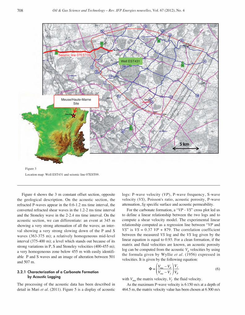
2D and 3D seismic data were recorded in France at theboundary of the Meuse and Haute-Marne departments in thevicinity of the Andra Center (National radioactive wastemanagement Agency). The acoustic data were recorded inwell “EST431” located on the Ribeaucourt township, in thenational forest of Montiers-sur-Saulx, 8 km North-North-West of the Andra Center. Figure 3 indicates the location ofthe seismic line “07EST09” and of the well “EST431”.

3.1 Geological Context

One of the drilling platforms, located in the center of thestudied zone, was used to study formations ranging fromOxfordian to Trias. The analysis presented here concernsborehole “EST431” and covers the Oxfordian formation. Theobjective of this borehole is to complement the geologicaland hydrogeological knowledge of this formation. This for-mation consists essentially of limestone deposited in a vastsedimentary platform (Ferry et al., 2007). The limestonefacies, which vary from one borehole to another, are gener-ally bio-detritic with reef constructions. In this formation,porosity ranges between 5 and 20% and “porous horizons” ofkilometric extension have been identified. As far as hydroge-ology is concerned the observed water inflows are usuallylocated in high porosity zones (Delay et al., 2007). The baseof the Kimmeridgian shale was observed at – 258.3 m (100 mASL) and the base of the Oxfordian limestone at – 544.3 m(–186 m ASL). During the drilling, water inflows weredetected at –368 m and – 440 m. At the end of the drilling,the well was left in its natural water.

3.2 Acoustic Logging

The acoustic tool used for the field experiment described inthis paper is a flexible monopole tool with two pairs ofreceivers: a pair of near receivers (1 and 1.25 m offsets) and apair of far receivers (3 and 3.25 m offsets). The source is amagnetostrictive transducer. The receivers are independentand each receiver has its own integrated acquisition device.The data have been recorded through the far offset configura-tion. The sampling depth interval is 10 cm. The sampling timeinterval is 5 microseconds. The length of recording is 5 ms.The acoustic log has been run in the Oxfordian carbonateformation, in the 333-510 m depth interval.


707

ogst120042_Mari 21/09/12 10:38 Page 707

Well EST431

Meuse/Haute-MarneSite

Seismic line 07EST09


Figure 3

Location map: Well EST431 and seismic line 07EST09.

Figure 4 shows the 3 m constant offset section, oppositethe geological description. On the acoustic section, therefracted P-waves appear in the 0.6-1.2 ms time interval, theconverted refracted shear waves in the 1.2-2 ms time intervaland the Stoneley wave in the 2-2.4 ms time interval. On theacoustic section, we can differentiate: an event at 345 mshowing a very strong attenuation of all the waves; an inter-val showing a very strong slowing down of the P and Swaves (363-375 m); a relatively homogeneous mid-levelinterval (375-400 m); a level which stands out because of itsstrong variations in P, S and Stoneley velocities (400-455 m);a very homogeneous zone below 455 m with easily identifi-able P and S waves and an image of alteration between 501and 507 m.

3.2.1 Characterization of a Carbonate Formationby Acoustic Logging

The processing of the acoustic data has been described indetail in Mari et al. (2011). Figure 5 is a display of acoustic

logs: P-wave velocity (VP), P-wave frequency, S-wavevelocity (VS), Poisson's ratio, acoustic porosity, P-waveattenuation, Sg specific surface and acoustic permeability.

For the carbonate formation, a “VP - VS” cross plot led usto define a linear relationship between the two logs and tocompute a shear velocity model. The experimental linearrelationship computed as a regression line between “VP andVS” is VS = 0.37 VP + 879. The correlation coefficientbetween the measured VS log and the VS log given by thelinear equation is equal to 0.93. For a clean formation, if thematrix and fluid velocities are known, an acoustic porositylog can be computed from the acoustic Vp velocities by usingthe formula given by Wyllie et al. (1956) expressed invelocities. It is given by the following equation:

(6)

with Vma the matrix velocity, Vf the fluid velocity.As the maximum P-wave velocity is 6150 m/s at a depth of

464.5 m, the matrix velocity value has been chosen at 6300 m/s

Φ =⎛

⎝⎜⎜

⎞

⎠⎟⎟

V V

V V

V

Vma P

ma f

f

P

–

–

ogst120042_Mari 21/09/12 10:38 Page 708

and the fluid velocity at 1 500 m/s, since the formation fluidis water. The acoustic porosity log, valid only in the cleanpart of the formation, shows a strong correlation (correlationcoefficient: 0.86) with a NMR (Nuclear Magnetic Resonance)porosity log (not displayed here) recorded in the well.

The attenuation (expressed in dB/m) of the formation iscomputed from the first eigensection (obtained by SVD) ofthe refracted P-wave acoustic signal recorded by the twoadjacent receivers of the acoustic tool. This point will bediscussed in the next section (Sect. 3.2.2).

Figure 5 (bottom right) shows the Sg specific surface logand the acoustic permeability log calculated from Equations

(4) and (5). The fluid viscosity μ and density ρf have beenassumed to be constant (μ = 1 centipoise, ρf = 1 g/cm3). Theacoustic permeability log detects three permeable zones at368 m, between 400 and 440 m, and 506 m. The permeablezone located at 506 m corresponds to a high value ofconductivity and is characterized by a low porosity (6%), a10 dB/m attenuation, but a significant decrease of the P-wavefrequency and of the specific surface. During drilling, waterinflows have been detected at –368 m and –440 m. At theend of the drilling, the well was left in its natural water. Thehydraulic tests and conductivity measurements conductedlater on did not confirm the inflow at 368 m seen during the


709

Coral and bioclastic packstone/grainstone

Shale

Wackstone with numerous corals and bioclasts, rare oolithic grainstone

Oolithic & bioclastic packstone/grainstone with a few oncolites

Oolithic packstone/grainstone with numerous corals

Oolithic grainstone with oncolites

Bioclastic packstone/grainstone

Oolithic and bioclastic grainstone translucent calcite at the bottom of the interval

5200.5

500

480

460

440

420

400

380

360

340

1.0 1.5Time (ms)

Dep

th (

m)

2.0 2.5

500

480

460

440

420

400

380

360

340

Figure 4

Acoustic logging and lithological description (Courtesy of Andra).

ogst120042_Mari 21/09/12 10:38 09


Well EST431: VP and Freq.-P logs

500

VP (m/s)

480

460

440

420

Dep

th (

m)

400

380

360

340

4000 6000Freq.-P (kHz)

10 20

500

Porosity

480

460

440

420

Dep

th (

m)

400

380

360

340

500

480

460

440

420

Dep

th (

m)

400

380

360

340

Well EST431: VS and Poisson’s ratio logs

500

VS (m/s)

480

460

440

420

Dep

th (

m)

400

380

360

340

30002000Poisson

0.2 0.3 0.4

500

480

460

440

420

Dep

th (

m)

400

380

360

340

0.1 0.2

500

Specific surface (m2/cm3)

480

460

440

420

Dep

th (

m)

400

380

360

340

1.88 1.89

500

K (mD)

480

460

440

420

Dep

th (

m)

400

380

360

340

0 2 4

500

Attenuation (dB/m)

480

460

440

420

Dep

th (

m)

400

380

360

340

100 20

Figure 5

Permeability estimation from acoustic logs (after Mari et al., 2011).

Top from left to right P-velocity and frequency logs; S-velocity and Poisson’s ratio logs.

Bottom from left to right porosity and attenuation logs; specific surface and predicted permeability (Ik-Seis) logs.

ogst120042_Mari 21/09/12 10:38 Page 710


711

drilling, but have validated the 400-440 m and 506 mpermeable zones detected by the acoustic logging.

A short pumping test was conducted between the 4thand 7th of March, 2008. This test, associated with fourgeochemical logs, highlighted five productive zones between– 297 and – 507 m. The overall productivity is weak with a15 L/min flow below 23.5 m drawdown. In general, there is agood correlation between the zones identified through theanalysis of the geochemical logs, the natural gamma-ray logand the NMR porosity log. All the identified productionzones correspond to low clay content zones.

The mean overall transmissivity of the Oxfordian belowthe EST431 drilling pad is 7.2 × 10-06 m2/s, ranging between5 × 10-06 and 1 × 10-05 m2/s. A total of five inflows have beenidentified between – 297.5 and – 506 m. The most productiveinflow (–506 m) ranges between 2.5 × 10-06 and 5 × 10-06 m2/s.These inflows are associated with pore porosity and correspondin part to the porous horizons described in the Oxfordianbelow the Underground Laboratory:– – 297.5 to – 301 m inflow, alternation of bioclastic and

oolites packstone/mudstone, which corresponds to HP7(L2c);

– – 328.5 m inflow, coral reefs packstone/grainstone, whichcorresponds to HP6 (L2b);

– – 413 m inflow, carbonated sand with oolites and oncolites,and numerous coral polyps, which corresponds to HP4(bottom of L1b);

– – 439 m inflow, oolites and coral polyps grainstone-packstone interface, which corresponds to HP3 (top of L1a);– 506 m inflow, oolites and coral polyps grainstone-

packstone interface, no correspondence with the poroushorizons (C3b). The acoustic porosity and free fluid NMRporosity do not exceed 6%. The inflow, detected by theacoustic permeability log, is characterized by a 10 dB/mattenuation, a significant decrease of the P-wave frequencyand of the specific surface.

The logs reveal a strong acoustic discontinuity at a depthof 345 m, clearly visible on the attenuation. The acousticdiscontinuity is also revealed by a strong increase of thespecific surface, a significant decrease of the acousticvelocities. The acoustic discontinuity is due to the presenceof a thin shaly layer in the carbonate formation. It isconfirmed by a change in the borehole diameter and a highvalue of the gamma ray log (not displayed here). Since at thatdepth, the acoustic porosity log has high values (larger than25%, Fig. 5 bottom left), the shaly layer is probably watersaturated.

3.2.2 Analysis of Refracted Acoustic Waves by SingularValue Decomposition (SVD)

The analysis of the acoustic waves recorded simultaneouslyon both receivers of the acoustic tool is used to computeadditional logs defined as acoustic attributes useful for the

characterization of the formation, such as amplitude, shapeindex and attenuation logs. The results obtained are optimumif the studied wave is extracted from the records and if thesignal to noise ratio is high. We show the benefit of usingSingular Value Decomposition (SVD) for that purpose. TheSVD processing is done on the 2 constant offset sectionsindependently, in a 5 traces (N = 5) depth running window.After flattening of each constant offset section with thepicked times of the refracted wave, the refracted wave signalspace is given by the first eigensection (NS = 1) obtained bySVD:

r=

sig = λ1 u1 v1T (7)

v1 is the first singular vector giving the time dependence,hence named normalized wavelet, u1 is the first singular vectorgiving the amplitude in depth, therefore called propagationvector and λ1 the associated eigenvalue. The amplitudevariation of the refracted wavelet over the depth interval isλ1u1.

Figure 6 (top left) shows the refracted wave signal spaceversus depth for the two constant offset sections associatedwith the two receivers (R1 and R2) of the acoustic tool. Thenoise space is the stack of the eigensections from rank 2 torank 5 (N = 5). The signal to noise ratio can be evaluated by:

(8)

and expressed in dB.The signal to noise ratio logs associated with the two

constant offset sections (R1 and R2) are shown in Figure 6(top right). We can notice a poor signal to noise in the shalylayer at 345 m and two anomalies near 390 m. Figure 6(bottom left) and Figure 7 (top) show for the two constantoffset sections (R1 and R2) the normalized wavelet (v1) andthe associated amplitude (λ1u1) log versus depth. Theamplitude logs have been used to compute the attenuation log(Fig. 5, bottom left) expressed in dB/m. The correlationcoefficient between the two normalized wavelets has beencomputed at each depth and the correlation coefficient log isshown in Figure 7 (bottom left). We can notice someanomalies at local depth (358, 390, 460, 492 and 503 m) anda significant decrease of the correlation coefficient in the400-440 m depth interval. The interval corresponds to theporous and permeable zone detected by the Ik-Seis factor(Fig. 5, bottom right). It is therefore suggested that changesin phase or distortion of the acoustic signal is linked topropagation through a porous and permeable zone. Thedistortions can be measured by a shape index attribute. Thestudy of the shape variation of the acoustic signals is notnew. Previous works have shown that this variation can beused to measure the attenuation of the formation and to detectcriss-cross patterns, fractures (Mari et al., 1996) andpermeable zones (Lebreton and Morlier, 1983; Lebreton andMorlier, 2010). To measure the shape variation, an acoustic

S N k

k

N

/ ==

∑λ λ1

2

/

ogst120042_Mari 21/09/12 10:38 Page 711


Acoustic logging: signal space

500

Time (ms)

R1

480

460

440

420

Dep

th (

m)

400

380

360

340

0.5 1.0

500

Time (ms)

R2 R1 R2

480

460

440

420

Dep

th (

m)

400

380

360

340

0.5 1.0

Signal to noise ratio

500

S/B (dB)

480

460

440

420

Dep

th (

m)

400

380

360

340

-20 0 20 40 -20 0 20 40

500

S/B (dB)

480

460

440

420

Dep

th (

m)

400

380

360

340

Wavelet analysis: amplitudes (receiver R2)

500

Amplitude A1

480

460

440

420

Dep

th (

m)

400

380

360

340

0.1

Wavelet analysis Wavelet R2

500

Time (ms) Lamda

480

460

440

420

Dep

th (

m)

400

380

360

340

1.00.5

500

Ic-R2

480

460

440

420

Dep

th (

m)

400

380

360

340

20000 5

500

480

460

440

420

Dep

th (

m)

400

380

360

340

500

Amplitude A2

480

460

440

420

Dep

th (

m)

400

380

360

340

0.1

500

Amplitude A3

480

460

440

420

Dep

th (

m)

400

380

360

340

0.1

Figure 6

Analysis of refracted waves in acoustic logging by Singular Value Decomposition (SVD).

Top from left to right: signal space and signal to noise ratio on the two receivers (R1 and R2) of the acoustic tool.

Bottom from left to right: wavelet and amplitude obtained by SVD, shape index, amplitudes of the first three arches of the wavelet (receiver R2).

ogst120042_Mari 21/09/12 10:38 Page 712


713


Acoustic logging: wavelet


500

Time (ms)

480

460

440

420

Dep

th (

m)

400

380

360

340

0.5 1.0

500

Time (ms)

480

460

440

420

Dep

th (

m)

400

380

360

340

0.5 1.0

500

Lamda

480

460

440

420

Dep

th (

m)

400

380

360

340

20000

500

Time (ms)

R1 R2

480

460

440

420

Dep

th (

m)

400

380

360

340

1.00.5

500

Time (ms)

480

460

440

420

Dep

th (

m)

400

380

360

340

0.5 1.0

500

Cor. coef.

480

460

440

420

Dep

th (

m)

400

380

360

340

0.8

500

Ic-R1

480

460

440

420

Dep

th (

m)

400

380

360

340

5

500

Lamda

480

460

440

420

Dep

th (

m)

400

380

360

340

20000

500

Ic-R2

480

460

440

420

Dep

th (

m)

400

380

360

340

540000

1.0

500

Ik-Seis

480

460

440

420

Dep

th (

m)

400

380

360

340

0 5

500

Ic

480

460

440

420

Dep

th (

m)

400

380

360

340

0 10

500

Cor. coef.

480

460

440

420D

epth

(m

)

400

380

360

340

0.8 1.00.9

Figure 7

Analysis of refracted waves in acoustic logging by Singular Value Decomposition (SVD).

Top from left to right: signal spaces (wavelet, amplitude, shape index) on receivers R1 and R2.

Bottom from left to right: wavelet R1, wavelet R2, correlation coefficient log, predicted permeability (Ik-Seis) and shape index logs.

ogst120042_Mari 21/09/12 10:38 Page 713

attribute, named Ic, independent of the energy of the source,has been introduced (Dupuy and Morlier, 1973; Lebreton andMorlier, 1983). The Ic parameter is given by the followingequation:

Ic = ((A2 + A3)/A1)n (9)

where A1, A2 and A3 are the amplitudes of the first threearches, respectively, of the studied signal and n an exponent.

Figure 6 (bottom left) shows the shape index Ic-R2 logcomputed from the amplitude logs (A1, A2 and A3, Fig. 6bottom right) associated with the normalized wavelet R2.The shape index is computed from formula (9) with anexponent value of 3 (n = 3). Figure 7 (top) allows the com-parison between the two shape index logs (Ic-R1 and Ic-R2).The shape index logs highlight anomalic zones, in the350-380 m depth interval with a maximum value at 358 m,and in the 400-440 m depth interval with a pick at 415 mwhich corresponds to the porous layer HP4. In order to reducethe noise to extract the common component of the two shapeindex logs (Ic-R1 and Ic-R2), the geometric mean of the twohas been computed. The resulting shape index log Ic iscompared with the Ik-Seis log and the correlation coefficientlog (Fig. 7, bottom right). The comparison shows a goodcoherence between the Ic log and the correlation coefficientlog. The permeable and porous layers in the 400-440 m depthinterval and the inflow at 506 m are seen both by the shapeindex log and by the Ik-Seis log. Shape index and correlationcoefficient logs can be used as a quick look method to detectpermeable bodies and inflows which must be confirmed bythe Ik-Seis log.

3.3 Seismic Surveying

The 2D seismic line was recorded in 2007 (see location map,Fig. 3). The 2D design is a split dip spread composed of240 traces. The distance between 2 traces is 25 m. The sourceis a vibroseis source generating a signal in the 14-140 Hzfrequency bandwidth. The bin size is 12.5 m. The nominalfold is 120.

3.3.1 Seismic Procedure

A conventional seismic sequence was applied to the data set.It includes amplitude recovery, deconvolution and waveseparation, static corrections, velocity analysis, CMP (CommonMid Point)-stacking and time migration.

However, the amplitude recovery has been done in twomain steps: spherical divergence compensation by using theNewman’s rule (1973) and attenuation compensation.Besides amplitude changes at each interface, the signalundergoes a general decay as a function of the propagationdistance from the source (decaying as 1/r) and with itstransmission through the interface. The application of a gain

scalar that is a function of t can compensate for these effects.Newman’s rule is commonly used. The decay rule proposedby Newman is:

1/Gs(t) = V1/(t.V2rms(t))

and consequently the gain function is:

Gs(t) = t.V2rms(t)/V1 (10)

where t is propagation time, V1 is the propagation velocity ofsound in the first layer and Vrms(t) is the rms velocity at time t.

In order to be able to apply the Newman’s law, the velocitymodel given by the rms velocity model must be estimated byvelocity analysis. An a priori gain scalar tV is applied to eachshot point. The deconvolution is then performed by spectrumequalization in the 10-130 Hz frequency band. The waveseparation by frequency – wavenumber filter (f-k filter) isthen done to cancel the direct, refracted and surface wavesand to enhance the reflected waves. The data are sorted inCMP gathers and the velocity analysis is performed. Theknowledge of the velocity model allows the computation ofthe gain function Gs(t). The initial gain function is retrievedand replaced by the function Gs(t). After such a processing,a residual decay of the amplitude of the stacked traces hasbeen noticed. The residual decay observed on the envelopeof the stacked trace has been used to extract a residualcompensation law Gr(t), after a strong smoothing in timeof the envelope. The amplitude recovery residual law hasbeen then approximated locally by an exponential law eαt,where t is propagation time and α attenuation factor. Figure 8(top, left) shows the stacked trace at CMP 600 after ampli-tude recovery by Newman’s law, the amplitude recoveryfunction which is used to compensate the attenuation and theseismic trace after compensation of attenuation.

The migrated section has been filtered by SVD in order toenhance the signal to noise ratio before computing seismicattributes (instantaneous frequency and envelope). BeforeSVD filtering, the migrated section has been shifted in timeto flatten a reference seismic horizon, noted S1. In that case,the SVD processing is done in the migrated section, in a 5traces (N = 5) CMP running window and the signal space iscomposed of the two first eigensections in order to take intoaccount the local dips which can been present in the timemigrated section. Figure 8 (top, right) shows the amplituderecovery function Gr(t), the instantaneous frequency trace f(t)and the associated Q function. The Q factor at time t isobtained from the following equation:

Q(t) = πf(t)/α with α = Ln (Gr(t))/t (11)

After migration, a model-based stratigraphic inversion (apriori impedance model obtained from well data) provides a2D impedance model section. The 2D impedance modelsection has also been shifted in time to flatten the seismichorizon S1. At well locations, the logs of velocity Vp, densityρ and porosity ϕ have been used to define laws between


ogst120042_Mari 21/09/12 10:38 Page 714


715

Seismic traces before and after amplitude recovery

0.7

0.6

0.5

0.4

0.3

0.2

0.1

0

Amplitude

Before

Tim

e (s

)

0

Permeability indicator

0.7

0.6

0.5

0.4

0.3

0.2

0.1

0

Imp. (g/cm3.m/s)

Tim

e (s

)

10000

0.7

0.6

0.5

0.4

0.3

0.2

0.1

0

Specific surface

Tim

e (s

)

0.5

0.7

0.6

0.5

0.4

0.3

0.2

0.1

0

Ik-Seis

Tim

e (s

)

1

Q estimation

0.7

0.6

0.5

0.4

0.3

0.2

0.1

0

Amplitude rec. functionTi

me

(s)

10

0.7

0.6

0.5

0.4

0.3

0.2

0.1

0

Frequency (Hz)

CMP gather 600

Tim

e (s

)

50

0.7

0.6

0.5

0.4

0.3

0.2

0.1

0

Q

Tim

e (s

)

100100

0.7

0.6

0.5

0.4

0.3

0.2

0.1

0

Amplitude rec. function

Tim

e (s

)

10

0.7

0.6

0.5

0.4

0.3

0.2

0.1

0

Amplitude

After

Tim

e (s

)

0

Available wells

25

20

Porosity = 45.1097 – 0.0028 impedance

Model equation

Por

osity

15

8000 9000Impedance

10000 11000

HTM102

EST 104

EST 201

EST 203

EST 204

EST 205

CMP gather 600

Figure 8

Seismic analysis at CMP 600. Top from left to right: seismic trace before and after amplitude recovery, amplitude recovery function, instantaneous frequency trace and Qseismic trace. Bottom from left to right: acoustic impedance trace, specific surface and Ik-Seis traces, porosity – acoustic impedance relationship.

ogst120042_Mari 21/09/12 10:38 Page 715


porosity and acoustic impedance (ϕ versus Ip) and between Vpand Ip. The porosity versus impedance cross-plot, displayed inFigure 8 (bottom right) was used to define a linear lawbetween the two. The porosity law obtained in the Oxfordianlimestone and the relation between Vs and Vp (Vs = 0.37 Vp+ 879) defined at well EST431 allow the computation of boththe pseudo specific surface and Ik-Seis functions, thanks toEquations (4) and (5) (Fig. 8, bottom left).

Figures 9 and 10 show the procedure of residual amplituderecovery and Q factor estimation for the seismic line“07EST09”. One can see the acoustic impedance section (Fig. 9,top left) and the variations of the residual amplitude recoverylaw Gr(t, n) along the seismic line, where t is propagation timeand n CMP number (Fig. 9, top right). As quality control, theeffect of amplitude recovery for attenuation can be clearlyseen on the envelops of the migrated section before and after

application of the Gr(t, n) law (Fig. 9, bottom). Aftercomputation of the instantaneous frequency section, Equation(11) is used to compute the Q factor section (Fig. 10). FinallyEquations (4) and (5) allow the computation of Ik-Seissections. The results are shown in the vicinity of CMP 600 inFigure 11 and for the total line in Figure 12.

3.3.2 Seismic Analysis at CMP 600

Figure 8 (bottom left) displays, at location of CMP 600, theacoustic impedance trace, the pseudo specific surface seismictrace with its associated Ik-Seis trace. The specific surfaceseismic trace clearly shows the main geological units: theKimmeridgian clay (between 0.1 and 0.2 s), the Oxfordiancarbonates (between 0.2 and 0.33 s), the Callovo Oxfordianclaystone (between 0.33 and 0.42 s), the Dogger carbonates

1000 15005000

Tim

e (s

)

0.15

0.20

0.25

0.30

0.35

0.40

0.45

0.50

0.55

2000

2500

1000

500

1500

c)

CMP

Envelop before Q compensation

1000 15005000

Tim

e (s

)

0.15

0.20

0.25

0.30

0.35

0.40

0.45

0.50

0.55

8000

7000

6000

5000

4000

3000

2000

1000

CMP

Envelop after Q comprensation

1000 15005000

Tim

e (s

)

0.15

0.20

0.25

0.30

0.35

0.40

0.45

0.50

0.55

16000

14000

12000

10000

8000

6000

a)

d)

b)

CMP

Acoustic impedance section

1000 15005000

Tim

e (s

)

0.15

0.20

0.25

0.30

0.35

0.40

0.45

0.50

0.55

10

9

8

7

6

5

4

3

CMP

Amplitude recovery function

Ip (g/cm3.m/s)

Figure 9

Seismic analysis: amplitude recovery. a) Acoustic impedance seismic section. b) Amplitude recovery function section.c) Envelop seismic sections before amplitude recovery. d) Envelop seismic sections after amplitude recovery.

ogst120042_Mari 21/09/12 10:38 Page 716

(between 0.42 and 0.53 s) and the Toarcien claystone after0.53 s. The shaly units have a high pseudo specific surfaceand a low value of the Ik-Seis factor. Figure 11 shows themigrated section and the associated Ik-Seis section in thevicinity of the CMP 600. As far as hydrogeology is con-

cerned the observed water inflows are usually located in highporosity zones located in the lower part of the Oxfordianlimestone, as it can be seen on the Ik-Seis section between0.28 and 0.33 s (Fig. 11a). The Ik-Seis section also shows thedistribution of the permeable bodies in the Dogger (Fig. 11b).


717

500 10000

Tim

e (s

)

0.15

0.55

0.50

0.45

0.40

0.35

0.30

0.25

0.20

110

100

90

80

70

60

50

40Hz

a)

CMP

Instantaneous frequency

1500 500 10000

Tim

e (s

)

0.15

0.55

0.50

0.45

0.40

0.35

0.30

0.25

100

90

80

70

60

50

40

30Q

b)

CMP

Q factor

1500

560 580 600 640620

560 580 600 640620

Tim

e (s

)

0.15

0.35

0.30

0.25

0.20

0.9

0.8

0.7

0.6

0.5

0.4

0.3

0.2

0.1

Tim

e (s

)

0.15

0.35

0.30

0.25

0.20

a)

CMP

Migrated section

CMP

Ik-Seis section

560 580 600 640620

Tim

e (s

)

0.35

0.55

0.50

0.45

0.40

CMP

Migrated section

CMP gather 600

560 580 600 640620

0.9

1.0

0.8

0.7

0.6

0.5

0.4

0.3

0.2

0.1

Tim

e (s

)

0.35

0.55

0.50

0.45

0.40

b)

CMP

Ik-Seis sectionCMP gather 600

Figure 10

Instantaneous frequency and Q-factor seismic sections.

Figure 11

Migrated and Ik-Seis sections at the vicinity of the CMP 600. a) 150-400 ms time interval, b) 350-600 ms time interval.

ogst120042_Mari 21/09/12 10:38 Page 717


3.3.3 Seismic Line Analysis

Figure 12 shows the distribution of the permeable bodies inthe carbonate formations via the Ik-Seis factor.

Several carbonated shelves have been emplaced duringthe middle and upper Jurassic, according to second orderstratigraphic sequences. The Callovo-Oxfordian argillite isdeposited over the Bathonian platform and is in turn overlaidby the Oxfordian platform.

The contact between the Dogger formation and theCallovo-Oxfordian argillite is sharp, associated toretrogradation condensed facies. The Dogger formationdisplays discontinuous thin porous layers in Figure 12 but thecorrelation with the two known thin porous layers cannot beassumed due to the seismic vertical resolution.

The Callovo-Oxfordian argillite displays very low valuesof the Ik-Seis factor, with no significant lateral variation ingood agreement with the known lithology. A carbonatedlayer, corresponding to a sequence boundary, has been used

for flattening. This layer is a known marker-bed in the Parisbasin (RIO: repère inférieur oolithique).

The value of the factor in the lower part of the Oxfordianlimestone (around 0.30 s) is low in the interval CMP 850-1600 according to the transition from high energy inner rampcarbonated facies toward outer ramp marly facies in the westdirection. The porosity decreases drastically in the westernfacies.

CONCLUSION

Knowledge about porosity and permeability is essential toevaluate fluid content and to detect fluid flow. We havepresented a procedure which allows to use geophysical data(i.e. full waveform acoustic data and reflection seismic data)for a better understanding of the distribution of the porousand permeable bodies. The methodology is based onlaboratory experiments which have shown that a formation

0 500

E W

1

2

3

4

Marne fault

1000 1500

Tim

e (s

)

0.15

0.20

0.25

0.30

0.35

0.40

0.45

0.50

0.55

0.1

0.2

0.3

0.4

0.5

0.6

0.7

0.8

0.9

1.0

Ik-Seis section

CMP

Figure 12

Ik-Seis section. 1: base of the Callovo-Oxfordian argillite; 2: carbonated layer used for flattening (S1); 3: top of the Callovo-Oxfordianargillite; Interval 3-4: Oxfordian limestone.

ogst120042_Mari 21/09/12 10:38 Page 718


719

permeability indicator, named Ik-Seis factor in the paper, canbe obtained via the computation of 4 quantities: P-wavefrequency, attenuation, porosity and specific surface.

The ability to use laboratory results for field geophysicalapplications has been discussed. The frequency content isimportant. Regarding frequencies above 2 kHz, permeabilityhas an influence on velocities and attenuations. The attenua-tion may reach a maximum for frequency in the order of10 kHz, this being the domain of full waveform acoustic logs.

Consequently, the procedure has been firstly conducted inacoustic logging to estimate the permeability of porous layersand to detect water inflows. Full waveform acoustic data wererecorded in an Oxfordian carbonate formation. The Ik-Seisfactor computed in the acoustic frequency domain (rangingbetween 10 and 25 kHz) has detected permeable zones, bothassociated with high porosity (20%) but also with low porosity(6%). The hydraulic tests and conductivity measurementsconducted later on have validated the permeable zonesdetected by acoustic logging. The benefit of using the SVDmethod to evaluate the signal to noise ratio, to compute theattenuation log and to extract the acoustic wavelets from theacoustic data has been shown. It has also been observed thatthe correlation coefficient computed between acoustic waveletsrecorded by two adjacent receivers of an acoustic toolsignificantly decreases in porous and permeable zones. It istherefore suggested that changes in phase or distortion of theacoustic signal is linked to propagation through a porous andpermeable zone. The distortions can be measured by a shapeindex attribute. After calibration on core data or hydraulic tests,the Ik-Seis could be seen as a pseudo acoustic permeability log.

In seismic, after signal to noise ratio enhancement by theSVD method, processing is carried out in order to measurethe needed parameters (frequency, attenuation, impedance) tocompute the Ik-Seis factor. The analytic signal is used tocompute the instantaneous frequency and attenuation (Qfactor). The porosity and specific surface are computed fromseismic impedances obtained by acoustic inversion of themigrated seismic sections. The Ik-Seis factor should only beused as a relative indicator which varies from 0 for less porousand permeable bodies to 1 for more porous and permeablebodies.

Our results suggest that it is possible to extract a significantIk-Seis factor from seismic sections. This factor leads to abetter understanding of the distribution of the porous andpermeable bodies. The potential of the proposed procedurehas been demonstrated via a 2D seismic profile. Theprocedure will be extended to 3D data.

ACKNOWLEDGMENTS

We thank Andra for permission to use the data presented inthe field examples. We thank Jean-Paul Sarda, Béatrice Yven

and Jean-Luc Bouchardon for their valuable help and advices.We thank Francisque Lebreton, Jean Dellenback and PierreGaudiani for very useful discussions on various occasions,specifically for their experience in acoustic logging.

REFERENCES

Biot M.A. (1956) Theory of propagation of elastic waves in a fluid-saturated porous solid, J. Acoust. Soc. Am. 28, 2, 168-191.

Bourbié Th., Coussy O., Zinszner B. (1987) Acoustics of PorousMedia, Editions Technip, ISBN 2-7108-0516-2, Paris.

Delay J., Rebours H., Vinsot A., Robin P. (2007) Scientific investi-gation in deep wells for nuclear waste disposal studies at theMeuse/Haute-Marne underground research laboratory, NortheasternFrance, Phys. Chem. Earth Parts A/B/C 32, 42-57.

Dupuy M., Lebreton F., Sarda J.P. (1973) Étude numérique del’influence de l’atténuation dans les roches sur la forme des signauxacoustiques, Transaction of the 2nd International FormationEvaluation Symposium, paper 4, SPWLA (SAID), Paris.

Fabricius I.L., Baechle G., Eberli G.P., Weger R. (2007) Estimatingpermeability of carbonate rocks from porosity and Vp/Vs,Geophysics 72, 5, 185-191, doi: 10.1190/1.2756081.

Ferry S., Pellenard P., Collin P.-Y., Thierry J., Marchand D.,Deconinck J.-F., Robin C., Carpentier C., Durlet C., Curial A.(2007) Synthesis of recent stratigraphic data on Bathonian toOxfordian deposits of the eastern Paris Basin, Mémoires de laSociété Géologique de France, Mém. Soc. Géol. Fr. n.s. 178, 37-57.

Gassmann F. (1951) Elastic waves through a packing of spheres,Geophysics 16, 673-685.

Glangeaud F., Mari J.L. (2000) Signal Processing in Geosciences,CD, Editions Technip, ISBN 2-7108-0768-8, Paris, France.

Klimentos T., McCann C. (1990) Relationships among compres-sional wave attenuation, porosity, clay content and permeabilitysandstones, Geophysics 55, 8, 998-1014.

Kozeny J. (1927) Über kapilläre Leitung des Wassers im Boden,Sitzungsberichte der Wiener Akademie der Wissenschaften 136,271-306.

Lebreton F., Morlier P. (1983) A permeability acoustic logging,Bull. Int. Assoc. Eng. Geol. 1, 101-105.

Lebreton F., Morlier P. (2010) Development of permeability loggingtechnique by recurrent alternating pressures in compacted clay rock,Transaction of the 4th international meeting Clays in Natural andengineered barriers for radioactive waste confinement, Nantes,March 29 - April 1st, Paper P/MT/CT/02, pp. 651-652.

Mari J.L., Delay J., Gaudiani P., Arens G. (1996) Geological forma-tion characterization by Stoneley waves, Eur. J. Environ. Eng.Geophys. 2, 1, 15-45.

Mari J.L., Gaudiani P., Delay J. (2011) Characterization of geologicalformations by physical parameters obtained through full waveformacoustic logging, Phys. Chem. Earth 36, 17, 1438-1449,doi:10.1016/j.pce.2011.07.011.

Mari J.L., Delay F. (2011) Contribution of seismic and acousticmethods to reservoir model building, in Hydraulic Conductivity -Issues, Determination and Applications / Book 1, InTech-OpenAccess Publisher, Chapter 17, ISBN 978-953-307-288-3.

Morlier P., Sarda J.P. (1971) Atténuation des ondes élastiques dansles roches poreuses saturées, Revue de l’Institut Français du Pétrole26, 9, 731-755.

Mortensen J., Engstrom F., Lind I. (1998) The relation amongporosity, permeability, and specific surface of chalk from the Gormfield, Danish North Sea, SPE Reserv. Evalu. Eng. 1, 245-251.

ogst120042_Mari 21/09/12 10:38 Page 719


Copyright © 2012 IFP Energies nouvellesPermission to make digital or hard copies of part or all of this work for personal or classroom use is granted without fee provided that copies are not madeor distributed for profit or commercial advantage and that copies bear this notice and the full citation on the first page. Copyrights for components of thiswork owned by others than IFP Energies nouvelles must be honored. Abstracting with credit is permitted. To copy otherwise, to republish, to post onservers, or to redistribute to lists, requires prior specific permission and/or a fee: Request permission from Information Mission, IFP Energies nouvelles,fax. +33 1 47 52 70 96, or [email protected].

Murphy W.F. III (1982) Effects of partial water saturation onattenuation in sandstones, J. Acoust. Soc. Am. 71, 1458-1468.

Newman P. (1973) Divergence effects in a layered earth,Geophysics 38, 377-406.

Plona T.J. (1980) Observation of a second bulk compressionnalwave in a porous medium at ultrasonic frequencies, Appl. Phys.Lett. 36, 259-261.

Schmitt D.P. (1986) Simulation numérique de diagraphies acoustiques,propagation d’ondes dans des formations cylindriques axisymétriquesradialement stratifiées incluant des milieux élastiques et/ou poreuxsaturés, Thèse, Grenoble, France.

Timur A. (1968) An investigation of permeability, porosity andresidual water saturation relationships, paper J, Spwla 9th AnnualLogging Symposium, June 23-26, Society of Petrophysicists andWell-Log Analysts.

Wyllie M.R., Gregory R.J., Gardner H.F. (1956) Elastic wave veloc-ities in heterogeneous ans porous media, Geophysics 21, 1, 41-70.

Yamamoto T. (2003) Imaging permeability structure within thehighly permeable carbonate earth: inverse theory and experiment,Geophysics 68, 4, 1189-1201, doi: 10.1190/1.1598103.

Zinszner B., Pellerin F.-M. (2007) A geoscientist’s guide to petro-physics, Editions Technip, ISBN 978-2-7108-0899-2, Paris.

Final manuscript received in February 2012Published online in September 2012

ogst120042_Mari 21/09/12 10:38 Page 720


721

APPENDIX: SINGULAR VALUE DECOMPOSITION (SVD)

Seismic or acoustic signals, recorded on an array of scalar sensors (singular component sensor) are generally described assummation of several events related to the different sources (reflected, refracted, converted waves, surface waves) propagatingthrough the media. The observed scalar signal depending on time t and space x (a seismic record) is described as:

(1)

where ai(t) is the wavelet of source i, si(t,x) the propagation vector of the source and * the symbol for the convolution product.Signal r(t,x) can be described in dual domains associated to time and distance variables as:

• Si(f,x) = FTt[si(t,x)], the distance – frequency space representation;

• Si(f,k) = FTx[Si(f,x)], the frequency – wavenumber representation (2D Fourier transforms on time and distance variables).

After propagation through the media, the received signal ri(t) on sensor i results from the superposition of NS waves [a1(t), ...,aNS(t)] via the transfer functions si, p(t):

(2)

where bi(t) is a noise supposed to be Gaussian, white and centred and Nc the number of sensors. With signals sampled in time,we write the received signals in a data matrix as:

r=

= {rj,i|i = 1, …, Nc; j = 1, …, Nt] ∈ ℜNc×Nt (3)

The Singular Value Decomposition of the time-space data matrix r=

provides two orthogonal matrices u and v and one diagonalmatrix Δ

=made up of singular values. The initial data matrix is expressed as:

r=

= u=

Δ=

v=

T= λk uk vkT with N = {min Nc, Nt} (4)

where:

• u = [u1, ..., uk, ..., uN] is a Nc × N orthogonal matrix made up of left singular vectors uk giving the amplitude in the real case(amplitude and phase in the complex case), therefore called propagation vectors;

• v = [v1, ..., vk, ..., vN] is a Nt × N orthogonal matrix made up of right singular vectors vk giving the time dependence, hencenamed normalized wavelets;

• Δ=

= diag(λ1, ..., λk, ..., λN) a N × N diagonal matrix with the diagonal entries ordered λ1 > ... > λk > ... > λN > 0.

The product ukvkT is an Nc × Nt unitary rank matrix named the kth singular image of data matrix r

=. Therefore, r

=is given by the

sum of all the kth singular images multiplied by their correspondent kth singular values λ. The rank of the matrix r=

is thenumber of non-zero singular values in Δ

=. In the noise free case, if the recorded signals are linearly dependent (for example if

they are equal to within a scale factor; that means one wave with an infinite velocity) the matrix r=

is of rank one and the perfectreconstruction requires only the first singular image. If the Nc recorded signals are linearly independent, the matrix r

=is full rank

and the perfect reconstruction requires all singular images.

Using the SVD filter, separation between the signal and the noise subspace is given by:

r=

= r=

sig + r=

noise = λk uk vkT + λk uk vk

T (5)

The signal subspace r=

sig is characterized by the first NS higher singular images (associated to the first NS higher singularvalues). It gives roughly the waveform of the dominant wave, its energy and its amplitude repartition on the sensors. Thereminder subspace r

=noise contains the waves with a low degree of sensor-to-sensor correlation and the noise. In practice, before

performing the SVD filtering, a flattening operation on the initial data is applied to obtain an infinite apparent velocity for theselected wave. For refracted waves, the flattening pre-processing is obtained by time shifting the data, the time shifts arederived from the picking of the first arrival times.

k NS

N

= +

∑1k

NS

=

∑1

k

N

=

∑1

r t s t a b t ii i p p i

p

NS

( ) ( – ). ( ) ( ),= + =∫∑=

τ τ with 1

11, Nc

r t x a t s t xi i

i

( , ) ,= ( ) ∗ ( )∑

ogst120042_Mari 21/09/12 10:38 Page 721

detection of porous and permeable formations: from

Documents