detection of energy sinks and sources in the active...

Detection of energy sinks and sources in the active vibra-tory energy field of coupled structures and systems withfluid-structure interaction

P. Groba 1, J. Ebert 1, T. Stoewer 1, C. Schaal 2, J. Bos 2, T. Melz 2

1 BMW Group, Department of Structural Dynamics, Structure-borne Sound and Vibrations,Knorrstraße 147, 80788 Munich, Germanye-mail: [email protected]

2 TU Darmstadt, Research group System Reliability and Machine Acoustics SzM,Magdalenenstraße 4, 64289 Darmstadt, Germany

AbstractIn this paper, an approach to obtain a holistic description of the acoustic chain of effects in a system withfluid-structure interaction based on energy quantities is considered. The approach is based on sound intensityand structural intensity. Both quantities offer detailed information about the propagation of the energy flow.The divergence of the structural intensity is introduced as a quantity that provides detailed information aboutthe location of energy sources and the structure’s behaviour in areas where energy is dissipated. To provethe ability of the divergence to identify sources and sinks, an analysis is conducted on a simply supportedrectangular plate. A simple approach to examine the energy transfer between subsystems in a coupled struc-ture is defined and its potential is illustrated in a simple example. For this purpose the divergence calculationis applied to a structure consisting of three plates, where a smaller plate in the middle serves as connectionbetween two bigger plates. Furthermore, the mutual reaction between the divergence of structural and soundintensity is analysed. The studies of the divergence of the acoustic intensities show their potential to obtaina more detailed knowledge of the acoustic chain of effects.

1 Introduction

One main target of NVH examinations of a machine structure, such as a car body, is to characterise themechanisms that lead from any excitation to its respective outcomes in terms of sound pressure and noise.The predictability and understanding of processes that are associated with this topic gain importance sincethe acoustic properties of the car are becoming more important for the customer’s satisfaction.

Since the first work of NOISEUX [1] in 1970 and the analytical description of simple structures by means ofPAVIC [2] there have been several further studies related to the structural intensity. The structural intensity isa physical quantity that draws attention due to its ability to illustrate the energy flow in a structure in detail.An overview of the development and research concerning the structural intensity can be found in the PhDthesis of HERING [3]. In this paper, a holistic approach for the description of the energetic chain of effectsis presented. This approach expands the information gathered by means of the structural intensity on thevibratory energy flow and source locations. This is done by means of the calculation of its divergence toachieve a better identification of the energy sources and energy sinks in the structure. The divergence of thestructural intensity is further used to examine the ability to depict an energy transmission between coupledstructures.

In addition to the structural intensity the sound intensity is introduced. Both quantities are analogous sinceboth represent the density and the direction of the energy flow in its respective medium. The objective of

3945

Figure 1: Energy flow between coupled structures and the surrounding fluid, according to [5]

extending the studies to the fluid is to analyse the relation of the divergence of the intensity fields in theboundary layer between the structure and the fluid. It is expected to gain a deeper understanding of theprocesses that lead to an energy exchange between the structure and the fluid.

2 Describing the energy propagation

The vibratory energy flow from the excitation point to the recipient can be depicted by means of the energeticchain of effects as shown in Figure 1. To describe the energy flow in the structure from excitation to radiationthe structural intensity (STI) is available and widely used. The energetic link between the radiation of soundand its immission at the recipient’s position can be achieved by means of the use of the sound intensity (SI).In addition to the distinction between fluid and structure a differentiation between different machine parts ismade. In this way, it is taken into account that the vibratory energy often passes more than one structuralcomponent before its radiation into the surrounding fluid. Therefore, the energy transmission between thesesubsystems plays an important role regarding the energy propagation in the whole system.

2.1 Energy balance of the coupled system

The first law of thermodynamics states that the sum of all energy changes in a closed system is equal to zero[4]. For an elastic medium it provides an energy balance that includes the STI Is and the densities of theinput energy πin and the dissipated energy πdiss. Since a power balance for the complete system should beconsidered, the system boundary has to be extended into the surrounding fluid. Thus, the energy balance alsoincludes the SI If . For a system with structure-fluid interaction the change of the energy density e per timecycle is obtained by [5]∫∫∫

V

∂e(t)

∂tdV = −

∫∫As

Is(t)nsdA−∫∫Af

If(t)nfdA+

∫∫∫V

(πin − πdiss)dV. (1)

The integration boundaries in Equation (1) are the volume V and the boundary surface A consisting of thestructural share As and the fluid’s share Af . The intensity quantities are considered in the direction of theunit normal vector n. For a system in a steady-state the change of e is equal to zero. In the frequency domainEquation (1) results in

Ps,in(f) =

∫∫As

Is,a(f)nsdA+

∫∫Af

If,a(f)nfdA+ Ps,diss(f). (2)

Equations (1) and (2) enable the complete description of the energetic condition of a vibrating structure andits surrounding fluid.

3946 PROCEEDINGS OF ISMA2016 INCLUDING USD2016

2.2 Energy flow in solids

The analyses in this work are performed on structures under forced harmonic excitation in a steady-state.Thus, the calculations result in complex values. The complex STI Is is calculated in every point of thestructure by means of the cross-spectral density of the complex stress tensor S and the conjugate-complexvelocity vector v∗ [3, 6]. In the frequency domain the STI is expressed as

Is(f) = −1

2S(f) · v∗(f). (3)

In electrical engineering it is common to distinguish between the active and reactive parts of power. Anal-ogously, the STI can be separated into an active and a reactive component [3]. The active STI indicates thedensity and the direction of the energy flow within a structure. The real part is equal to the active STI and tothe STI in the time domain over a period T as follows

Is,a(f) = Re (Is(f)) = 〈Is(t)〉 =1

T

∫ T

0Is(t) dt. (4)

The brackets 〈〉 in Equation (4) indicate time-averaging. This means that the active part of the STI in thefrequency domain is directly related to the average value of the STI in the time domain. On the other hand,the reactive STI

Is,r(f) = Im (Is(f)) (5)

is controversial in its physical meaning [3]. Statements in the literature are that the reactive STI representsthe reversible part of the mechanical energy flux [7] or that it describes the local exchange of energy betweenthe kinetic and the potential energy component in the system [6]. The focus of this paper is on the active partof the STI.

2.2.1 The structural intensity in thin-walled structures

Concerning the sound radiation of machine surfaces the main sources of noise are the thin-walled structuralparts. Examples for thin-walled structures in the vehicle body are the doors, the roof, and the underbody.In order to depict the dynamic behaviour of thin-walled structures in an FE analysis these are modelled as ashell for which the KIRCHHOFF plate theory is valid. A shell section with its section forcesN , Q and sectionmoments M , as well as its translational and rotational velocities v, ϕ is shown in Figure 2. The formulationfor the STI in shells in the frequency domain is given by

I′(f) =

I ′xI ′yI ′z

= −1

2

Nxv∗x +Nxyv

∗y +Mxϕ

∗y−Mxyϕ

∗x

+Qxv∗z

Nyv∗y +Nyxv

∗x −Myϕ

∗x

+Myxϕ∗y

+Qyv∗z

0

, (6)

where the result is, in equivalence to Equation (3), gained through the use of the cross-spectral density. Theenergy flow in z-direction is small in comparison to the components in x- and y-direction and, therefore,I ′z is neglected [3]. The mathematical representation of I′(f) is analogous to the integration of Is(f) inEquation (7) over the thickness of the plate [6] in Equation (6)

I′(f) =

∫ h2

−h2

Is(f) dz. (7)

VIBRO-ACOUSTIC MODELLING AND PREDICTION 3947

Figure 2: Sketch of: a) section forces and moments and b) translational and rotatory components of thevelocity at a shell

2.3 Energy flow in fluids

In the fluid, the energy flow is described by the SI. In steady-state, it can be written as

If(f) =1

2p(f)v∗(f), (8)

where p is the complex pressure and v∗ the conjugate-complex of the particle velocity. As for the STI thetime-averaged value of the SI has a direct correlation with the real part of the steady-state value. It is givenby [8]

〈If(t)〉 =1

2Re(p(f)v∗(f)

). (9)

The time-averaged SI in steady-state can also be computed by means of integration over the period T

〈If(t)〉 =1

T

∫ T

0If(t)dt =

1

T

∫ T

0p(t)v(t)dt. (10)

3 Localisation of structural areas of power input and output

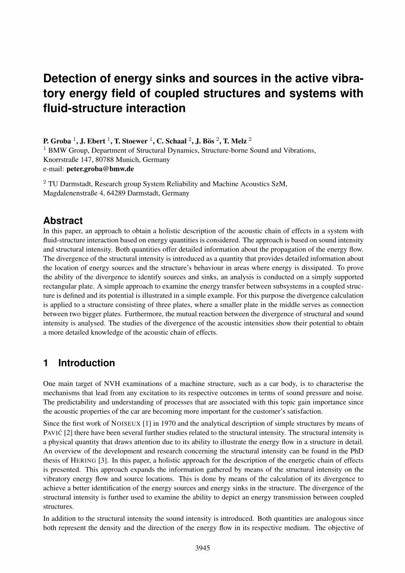
In literature, examples can be found to identify sources in the vibratory energy field by STI analysis. Someresearchers determine the position of the energy source by the behaviour of the STI vectors of the measuredvector field [9, 10]. In the example of a harmonically excited plate it will be shown why the informationgained by means of the STI vector field is not necessarily enough for this purpose. Therefore, the calculationsare carried out on a simply supported rectangular plate as shown in Figure 3. The rectangular plate has alength of lx = 0.86 m, a width of ly = 0.63 m, and a thickness of h = 0.004 m. It consists of aluminiumwith a YOUNG’s modulus of E = 7 · 1010 Nm−2, a density of % = 2700 kgm−3, a POISSON’s ratio ofµ = 0.34, and a structural loss factor of η = 1 · 10−3. A harmonic concentrated load of 1 N is applied atxF = yF = 0.16 m as shown in Figure 3. The plate is excited at its natural frequencies.

Figure 4 shows the results for the FE calculation of the plate excited at the 4th and 7th natural frequencies,which are almost identical to their corresponding resonance frequencies for lightly damped structures. Inthe following studies, the absolute value of the energy flow is the mainly analysed quantity. In case of theSTI the absolute value is called flux density (FD). For the 4th natural frequency of the plate, it is possible todetermine the source from the distribution of the STI. The highest value of FD (red area) shows the location


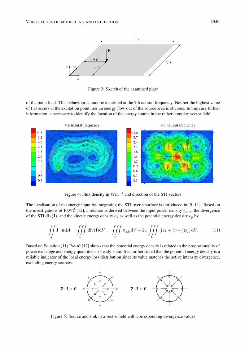
Figure 3: Sketch of the examined plate

of the point load. This behaviour cannot be identified at the 7th natural frequency. Neither the highest valueof FD occurs at the excitation point, nor an energy flow out of the source area is obvious. In this case furtherinformation is necessary to identify the location of the energy source in the rather complex vector field.

Figure 4: Flux density in Wm−1 and direction of the STI vectors

The localisation of the energy input by integrating the STI over a surface is introduced in [9, 11]. Based onthe investigations of PAVIC [12], a relation is derived between the input power density πs,in, the divergenceof the STI div(I), and the kinetic energy density ek as well as the potential energy density ep by∫∫

A

I · ndA =

∫∫∫V

div(I)dV =

∫∫∫V

πs,indV − 2ω

∫∫∫V

[j ek + (η − j)ep] dV. (11)

Based on Equation (11) PAVIC [12] shows that the potential energy density is related to the proportionality ofpower exchange and energy quantities in steady-state. It is further stated that the potential energy density is areliable indicator of the local energy loss distribution since its value matches the active intensity divergence,excluding energy sources.

Figure 5: Source and sink in a vector field with corresponding divergence values


In general, the divergence∇·I allows for the identification of sources and sinks in vector fields [13]. Figure 5shows exemplarily the direction of the vector fields by illustrating a source and a sink. It is depicted that incase of∇·I > 0 the considered area is a source and the vectors are diverging. On the other hand, if∇·I < 0the vectors are conjoining to a point, which represents a sink. The divergence of the STI is equal to the scalarproduct of the STI vector field with the nabla operator [12]

∇ · I =∂

∂xiIi =

∂I1

∂x1+∂I2

∂x2+∂I3

∂x3. (12)

In this paper, the divergence’s calculations based on Equation (12) are carried out by means of numericalderivation based on the central difference quotient. In the first conducted analyses the above mentionedproperties of the divergence and, thus, the suitability of the calculation approach are examined.

Figure 6: Divergence of the STI in Wm−2 and direction of the STI vectors

In Figure 6 the STI’s divergence for the 4th and 7th natural frequency is illustrated based on the STI vectorfield depicted in Figure 4. For both natural frequencies the position of the concentrated load can be clearlyidentified by the red area. The remaining plate has divergence values that are lower and mostly negative. Theused model’s damping is a rather small structural damping, which results in rather small differences in theSTI’s divergence outside the area of the external load.

Figure 7: Potential energy density and divergence of the STI of the 4th natural frequency

In order to examine the behaviour of the STI’s divergence besides the excitation point, the scale of the colourrange in Figure 6 must be adapted. This is done for the 4th natural frequency. The result for the scaled STI’sdivergence is shown on the right side of Figure 7. There are three regions with high negative values (greenareas). These regions indicate a high dissipation compared to the remaining plate, excluding the excitation


point. On the left side of Figure 7 the potential energy density, which, as already mentioned, also reveals thelocation of energy sinks, is shown. A comparison of the potential energy density and STI’s divergence leadsto the conclusion that the number and alignment of areas with a high potential energy density correspond toareas with a high negative STI’s divergence.

But it is also visible that the potential energy density does not indicate the presence of the energy source as theSTI’s divergence does. This is an advantage of the STI’s divergence because it includes the identification ofsources. Hence, the presented results are in accordance with the statements concerning the STI’s divergencein this section and the work done by PAVIC [12] and LAMARSAUDE [13].

However, the results of the STI’s divergence calculation exhibit a few discrepancies. Close to the boundariesas well as in the areas of low velocities, the divergence shows positive values (red areas). This behaviourstands in contrast to the theoretical considerations since no energy is inputted to the model at those areas.Furthermore, in the vicinity of the excitation point the result shows increased negative values (blue areas). Itwas stated earlier that the potential energy density is directly related to the dissipated energy. The potentialenergy density in Figure 7 shows no increased values in the area of the excitation point. This result leadsto the conclusion that in future studies the numerical implementation of the STI’s divergence according toEquation (12) needs to be analysed in order to identify possibilities for improvements or to eliminate theinaccuracies.

3.1 Calculation approach to approximate the energy transmission in coupled struc-tures

In this section, an approach to analyse the energy transmission between coupled structures is introduced. It isbased on the fact that the energy crosses a system boundary every time it is transmitted to another part of thestructure. This means if the energy leaves a regarded part, its divergence should indicate a sink. In contrast,the divergence should indicate a source if the energy enters the structure over a system’s boundary, which isthe same principle as the application of an external force. One of the main questions considering this prob-lem is whether it is necessary to calculate the STI and its divergence for every part of the system includingconnections such as welding spots, seams, or even more complex connection types such as bearings. Thiswould require the calculation of the STI and its divergence in connectors’ volume elements, which is a com-plicated task on its own. Since the focus is on the behaviour of thin-walled structures whose vibrations are themain reason for structure-borne sound radiation, it would be beneficial to limit the calculations to these parts.

Figure 8: Calculation approach: a) calculation process and b) sketch of thin-walled test structure with auxil-iary system boundaries

The question if the STI and its divergence must be calculated for all parts to represent the energy transmissionbehaviour is analysed in a thin-walled test structure as shown in Figure 8 b). This structure is divided by the


auxiliary system boundaries into three single plates, whereby the two identical plates on the left and the rightside are connected by a smaller plate in the middle called connection area.

For the identification of energy sources and sinks in the connection area the assumption is made that it issufficient to know the direction of the energy flow over a system’s boundary. If this is the case it is notnecessary to know the STI distribution in the structure’s connection area. In a first approximation it isassumed that the vibratory energy flow appears or disappears in the connection area, which is considereda black box. Therefore, the STI in the connection area is set to zero. This assumption can be realised bycalculating the STI’s divergence as shown in the right branch in Figure 8 a). The main requirement for thisapproach, in regard to more complex structures, is for the user to know where the connections are in themodel or to enable the calculation approach to identify these regions.

Figure 9: Calculation results for the 1st natural frequency of the test structure

The material properties and the outer dimensions of the used test structure are consistent with the platedepicted in Figure 3. The structure is also excited by a harmonic concentrated force with an amplitude of1 N on the right side. This is clearly visible in the upper left picture in Figure 9 (red area), which shows theresult of FD and the direction of the STI.

The subfigures in the lower part of Figure 9 show the results of the different divergence calculation ap-proaches as shown in Figure 8 a). On the left side, the STI’s divergence is calculated based on the unmod-ified STI’s distribution for model 1. As expected, it shows clearly the excitation point (red cross). Further,it is visible that most of the energy is dissipated on the right side of the structure since there the occurringnegative divergence values are substantially higher than on the left side of the structure. This behaviour is inaccordance to the qualitative distribution of the potential energy density in the upper right subfigure of Fig-ure 9. The potential energy density additionally shows high values in the corners of the connection area, a


behaviour that may result from occurring numerical singularities and, therefore, high stresses in the corner’svicinity. This effect seems to influence the quality of the calculated STI results and its divergence since thedivergence has positive values in this area. Since the only external force is applied on the excitation point ofthe test structure, these positive values resemble specious sources. The exact reason for the appearance ofthis phenomenon must be clarified in future studies. A main issue in further analyses will be the reliabilityof the calculation results of the STI and the divergence in peripheral areas.

The lower right subfigure in Figure 9 shows the result for the divergence calculation with the assumptionthat the STI is zero in the connection area (model 2 in Figure 8 a)). The impact of the additional step isconsiderably visible by comparing the results of the two different calculations of the STI’s divergence. Sincethe STI in the connection area is zero, the result for the divergence in this area is zero. This, however, is notthe case for the initial calculation result on the left side. There, the STI’s divergence in the connection area hasnegative values and, therefore, hints to energy dissipation due to structural damping. On the right part of thetest structure the vibratory energy flows into the connection area and leaves the right part of the test structure.The divergence indicates an energy sink at the right auxiliary boundary. At the left auxiliary boundary, thedivergence indicates a source since the energy flows from the connection area over the boundary into the leftpart of the test structure. For this simple example, the calculation shows that the divergence can correctlydepict energy sources and sinks at auxiliary system boundaries. The source and sink arrangement shows theexpected result since their order leads to the conclusion that the energy flows from the excited part of the teststructure (right side) through the connection area into the left side of the test structure. A further observationis that the values of the STI’s divergence at the auxiliary boundaries are increased. This is due to the strongdiscontinuity that is created by setting the energy flow level in the connection area to zero.

In this section it is visible that the divergence is a useful quantity to identify sources and sinks in fieldsof the vibratory energy flow and to gather information about areas of higher energy dissipation. The shownexample indicates that the divergence correctly identifies the energy sinks and sources at auxiliary boundariesbetween coupled parts. It must be clarified whether the shown approach is necessary and suitable when thecalculation method is applied to more complex cases.

4 Energy-based analysis of dynamic systems with fluid-structure in-teraction

In this chapter, the energy exchange is analysed for a dynamic system with fluid-structure interaction. Theanalysis is based on both acoustic intensities (structural intensity STI and sound intensity SI) and their di-vergences within such a dynamic system. The applied calculation approach is based on the real part ofEquation (11) and can be written as follows

div(Ia) = πin − 2ωηep. (13)

For the analyses in this chapter, Equation (13) is implemented and is an extension of the sole representation ofthe potential energy density ep exemplarily shown in the upper right subfigure of Figure 9. The divergence’scalculation approach shown in chapter 3 is expected to work for dynamic systems with fluid-structure inter-action, but it is actually not implemented. Equation (13) remains valid for the fluid of a dynamic system.

The exemplarily used dynamic system, in the further paper called acoustic box, consists of a rectangularplate and a fluid with the shape of a cuboid and is schematically shown in Figure 10. The plate has theidentical material properties as the test structure in chapter 3 and a size of lx · ly = 850 · 620 mm2. The fluidhas the same base area at the coupling surface as the plate and a height of lz = 550 mm shown in Figure 10.The fluid has the material properties of air (a bulk modulus of κf = 0.1418, a density of ρf = 1.204 kgm−3,and a damping from hysteresis of ηf = 2.532 · 10−6). The plate is coupled normal to the fluid’s couplingsurface. The acoustic box is harmonically excited at the plate by an external pressure load (an amplitude ofpz = 634.9 Nm−2 and a surface of 2000 mm2) and at the natural frequencies of the whole acoustic box.The middle of the excitation surface is located at the point x0 = 0.35 m, y0 = 0.22 m.


Figure 10: Schematic illustration of the acoustic box

In Figure 11 the acoustic intensities (STI and SI) and their divergences are shown for an excitation at the3rd (left column) and 6th (right column) natural frequency. Focusing on the STI’s divergence (first row ofFigure 11), the external pressure load can be identified as an energy source for both depicted natural fre-quencies (grey area). At the 6th natural frequency, it must be stated that the area of input power is largerthan the applied pressure load surface. The reason for it is an inaccurate interpolation from an element-wisescalar field to a continuous scalar field in the postprocessing tool. Additionally, the highest dissipated energydensity is located at the position of high structure’s velocities (blue area) for both selected excitations. Inthe second row of Figure 11, the SI’s divergence (colour) and the SI itself (vectors) are shown. Comparingthe SI’s divergence with the STI’s divergence, it attracts attention that at the 3rd natural frequency the diver-gences’ distributions are similar to each other, whereas both distributions completely differ at the 6th naturalfrequency. The reason is that the 6th natural frequency of the whole acoustic box is the fluid’s fundamentalfrequency. Hence, the vibration influence of the plate on the fluid is superposed by the deflection shape of thefluid. In contrast, at a fluid’s natural frequency the fluid’s dynamics do not influence the structure’s dynamicsas intensely as the structure’s dynamics influences the fluid’s dynamics at a structure’s natural frequency.This is caused by a big difference of the densities between structure and fluid [14]. Furthermore, it is appar-ent that the SI’s divergence has only negative values. Based on the implemented SI’s divergence accordingto Equation (13), the fluid is only acting as a sink at the coupling surface (dissipation), because no externalenergy source is located in the fluid. In the second row of Figure 11, the SI vectors show that active energyflow is taking place. This energy flow in the fluid would necessitate that a share of the complete vibratoryenergy flows from the structure into the fluid. This fact would implicate that energy sources must appear atthe fluid’s coupling surface. Finally, this means that the energy sources cannot be identified within a dynamicsystem with fluid-structure interaction at the fluid’s coupling surface based on Equation (13).

In the third row of Figure 11, the sound intensity itself at the fluid’s coupling surface normal to the plateis visualised. The scale of the SI has positive and negative values, which indicates the existence of sinks(blue areas) and sources (red areas). The regions of positive SI operate as a source (energy flows from thestructure to the fluid) and the regions of negative SI as a sink (energy flows from the fluid to the structure).In general, it can be stated that a high energy transfer (sinks and sources) occurs at those regions, where theplate’s vibration and/or the fluid’s excitability are high.

Finally, it can be summarised that only sinks that are directly related to dissipation can be located based onthe used calculation approach for the STI’s and SI’s divergence. For the identification of sinks and sourcesbetween structure and fluid, the sound intensity normal to the plate at the coupling surface is a suitableapproach. An application of the divergence calculation based on the central difference quotient is moresuitable and would hold out that sinks and sources between the structure and the fluid could be identifiedincluding the dissipation’s influence.


Figure 11: STI and its divergence at the plate as well as the SI and its divergence at the coupling surface ofthe acoustic box excited at the 3rd and 6th natural frequency

5 Conclusion

The work presented in this paper is performed to deepen the knowledge about the processes involved in theacoustic chain of effects. Therefore, the structural intensity and the sound intensity are introduced in orderto describe the energy flow in the structure and the fluid. To enhance the gathered information about energytransfer in coupled systems the divergence of acoustic intensities is introduced.

With the first analyses, it is shown that the STI’s divergence can be used to identify energy sources and sinksand to predict areas of structures where high energy dissipation occurs. Further it is shown that the introducedcalculation approach based on the central difference quotient can additionally indicate the direction of theenergy flow over a system boundary. Hence, the STI’s divergence seems to be a suitable quantity to examinethe energy transmission in coupled structures in order to achieve a more detailed knowledge about the energyexchange in dynamic systems. Therefore, the introduced approaches will be extended to more complexmodels in future studies.

The analysis of the STI’s and SI’s divergences based on the potential energy density superposed with the inputpower density point out that only sinks related to material dissipation and sources of external excitations canbe identified. The energy transfer between the structure and the fluid is not identifiable by the implemented


divergences. Therefore, the sound intensity itself normal to the structure can be used at the fluid’s couplingsurface. In further studies, the calculation approach of the STI’s divergence based on the central differencequotient will be applied in an analogous way to the SI.

References

[1] D. U. Noiseux, Measurement of power flow in uniform beams and plates, Journal of the Acoustical Society of America, Vol. 47, No. 1 (1970), pp. 238-247.

[2] G. Pavic, Measurement of structure borne wave intensity, part1: Formulation of methods, Journal of Sound and Vibration, Vol. 49, No. 2 (1976), pp. 221-230.

[3] T. Hering, Strukturintensitatsanalyse als Werkzeug der Maschinenakustik, PhD thesis, Technische Uni-versitat Darmstadt (2012).

[4] T. L. Bergman, F. P. Incropera, D. P. DeWitt, A. S. Lavine, Fundamentals of heat and mass transfer, 7th edition, John Wiley & Sons, Hoboken (2011).

[5] J. Ebert, T. Stoewer, C. Schaal, J. Bos, T. Melz, Opportunities and limitations on vibro-acoustic design of vehicle structures by means of energy flow-based numerical simulations, in Proceedings of NOVEM 2015 Noise and Vibration - Emerging Technologies, Croatia, 2015 April 12-15, Dubrovnik (2015), pp. 49798-1-49798-16.

[6] S. Buckert, Bewertung adaptiver Strukturen auf Basis der Strukturintensitat, PhD thesis, Technische Universitat Darmstadt (2013).

[7] G. Pavic, Structural surface intensity - An alternative approach in vibration analysis and diagnosis, Journal of Sound and Vibration, Vol. 115, No. 3 (1987), pp. 405-422.

[8] G. H. Koopmann, J. B. Fahnline, Designing quiet structures: A sound power minimization approach, Academic Press, San Diego (1997).

[9] E. G. Williams, H. D. Dardy, R. G. Fink, A technique for measurement of structure-borne intensity in plates, Journal of the Acoustical Society of America, Vol. 78, No. 6 (1985), pp. 2061-2068.

[10]A. Nejade, R. Singh, Flexural intensity measurement on finite plates using modal spectrum ideal filter-ing, Journal of Sound and Vibration, Vol. 256, No. 1 (2002), pp. 33-63.

[11]A. J. Romano, P. B. Abraham, E. G. Williams, A Poynting vector formulation for thin shells and plates, and its application to structural intensity analysis and source localization. Part I: Theory, Journal of the Acoustical Society of America, Vol. 87, No. 3 (1990), pp. 1166-1174.

[12]G. Pavic, The role of damping on energy and power in vibrating systems, Journal of Sound and Vibra-tion, Vol. 281 (2005), pp. 45-71.

[13]B. Lamarsaude, Y. Bousseau, A. Jund, Structural intensity analysis for car body design: going beyond interpretation issues through vector field processing, in Proceedings of ISMA2014 including USD2014, Belgium, 2014 September 15-17, Leuven (2014), pp. 3677-3686.

[14]S. Herold, Simulation des dynamischen und akustischen Verhaltens aktiver Systeme im Zeitbereich, PhD thesis, Technische Universitat Darmstadt (2003).


detection of energy sinks and sources in the active...

Documents