Detection, Estimation, and Modulation Theory

This page intentionally left blank

Detection, Estimation,and Modulation Theory

Part I. Detection, Estimation,and Linear Modulation Theory

HARRY L. VAN TREESGeorge Mason University

A Wiley-Interscience PublicationJOHN WILEY & SONS, INC.

New York • Chichester • Weinheim • Brisbane • Singapore • Toronto

This text is printed on acid-free paper. ®

Copyright © 2001 by John Wiley & Sons, Inc. All rights reserved.

Published simultaneously in Canada.

No part of this publication may be reproduced, stored in a retrieval system or transmitted in anyform or by any means, electronic, mechanical, photocopying, recording, scanning or otherwise,except as permitted under Section 107 or 108 of the 1976 United States Copyright Act, withouteither the prior written permission of the Publisher, or authorization through payment of theappropriate per-copy fee to the Copyright Clearance Center, 222 Rosewood Drive, Danvers, MA01923, (978) 750-8400, fax (978) 750-4744. Requests to the Publisher for permission should beaddressed to the Permissions Department, John Wiley & Sons, Inc., 605 Third Avenue, New York,NY 10158-0012, (212) 850-6011, fax (212) 850-6008, E-Mail: PERMREQ@WILEY.COM.

For ordering and customer service, call 1-800-CALL-WILEY.

Library of Congress Cataloging in Publication Data is available.

ISBN 0-471-09517-6

Printed in the United States of America

1 0 9 8 7 6 5 4 3

To Diane

and Stephen, Mark, Kathleen, Patricia,Eileen, Harry, and Julia

and the next generation—Brittany, Erin, Thomas, Elizabeth, Emily,Dillon, Bryan, Julia, Robert, Margaret,Peter, Emma, Sarah, Harry, Rebecca,and Molly

This page intentionally left blank

Preface for Paperback Edition

In 1968, Part I of Detection, Estimation, and Modulation Theory [VT68] was pub-lished. It turned out to be a reasonably successful book that has been widely used byseveral generations of engineers. There were thirty printings, but the last printingwas in 1996. Volumes II and III ([VT71a], [VT71b]) were published in 1971 and fo-cused on specific application areas such as analog modulation, Gaussian signalsand noise, and the radar-sonar problem. Volume II had a short life span due to theshift from analog modulation to digital modulation. Volume III is still widely usedas a reference and as a supplementary text. In a moment of youthful optimism, I in-dicated in the the Preface to Volume III and in Chapter III-14 that a short mono-graph on optimum array processing would be published in 1971. The bibliographylists it as a reference, Optimum Array Processing, Wiley, 1971, which has been sub-sequently cited by several authors. After a 30-year delay, Optimum Array Process-ing, Part IV of Detection, Estimation, and Modulation Theory will be published thisyear.

A few comments on my career may help explain the long delay. In 1972, MITloaned me to the Defense Communication Agency in Washington, D.C. where Ispent three years as the Chief Scientist and the Associate Director of Technology. Atthe end of the tour, I decided, for personal reasons, to stay in the Washington, D.C.area. I spent three years as an Assistant Vice-President at COMSAT where mygroup did the advanced planning for the INTELSAT satellites. In 1978, I becamethe Chief Scientist of the United States Air Force. In 1979, Dr. Gerald Dinneen, theformer Director of Lincoln Laboratories, was serving as Assistant Secretary of De-fense for C31. He asked me to become his Principal Deputy and I spent two years inthat position. In 1981,1 joined M/A-COM Linkabit. Linkabit is the company that Ir-win Jacobs and Andrew Viterbi had started in 1969 and sold to M/A-COM in 1979.I started an Eastern operation which grew to about 200 people in three years. AfterIrwin and Andy left M/A-COM and started Qualcomm, I was responsible for thegovernment operations in San Diego as well as Washington, D.C. In 1988, M/A-COM sold the division. At that point I decided to return to the academic world.

I joined George Mason University in September of 1988. One of my prioritieswas to finish the book on optimum array processing. However, I found that I neededto build up a research center in order to attract young research-oriented faculty and

vn

viii Preface for Paperback Edition

doctoral students. The process took about six years. The Center for Excellence inCommand, Control, Communications, and Intelligence has been very successfuland has generated over $300 million in research funding during its existence. Dur-ing this growth period, I spent some time on array processing but a concentrated ef-fort was not possible. In 1995,1 started a serious effort to write the Array Process-ing book.

Throughout the Optimum Array Processing text there are references to Parts Iand III of Detection, Estimation, and Modulation Theory. The referenced material isavailable in several other books, but I am most familiar with my own work. Wileyagreed to publish Part I and III in paperback so the material will be readily avail-able. In addition to providing background for Part IV, Part I is still useful as a textfor a graduate course in Detection and Estimation Theory. Part III is suitable for asecond level graduate course dealing with more specialized topics.

In the 30-year period, there has been a dramatic change in the signal processingarea. Advances in computational capability have allowed the implementation ofcomplex algorithms that were only of theoretical interest in the past. In many appli-cations, algorithms can be implemented that reach the theoretical bounds.

The advances in computational capability have also changed how the material istaught. In Parts I and III, there is an emphasis on compact analytical solutions toproblems. In Part IV, there is a much greater emphasis on efficient iterative solu-tions and simulations. All of the material in parts I and III is still relevant. The booksuse continuous time processes but the transition to discrete time processes isstraightforward. Integrals that were difficult to do analytically can be done easily inMatlab®. The various detection and estimation algorithms can be simulated andtheir performance compared to the theoretical bounds. We still use most of the prob-lems in the text but supplement them with problems that require Matlab® solutions.

We hope that a new generation of students and readers find these reprinted edi-tions to be useful.

HARRY L. VAN TREESFairfax, VirginiaJune 2001

Preface

The area of detection and estimation theory that we shall study in this bookrepresents a combination of the classical techniques of statistical inferenceand the random process characterization of communication, radar, sonar,and other modern data processing systems. The two major areas of statis-tical inference are decision theory and estimation theory. In the first casewe observe an output that has a random character and decide which of twopossible causes produced it. This type of problem was studied in the middleof the eighteenth century by Thomas Bayes [1]. In the estimation theorycase the output is related to the value of some parameter of interest, andwe try to estimate the value of this parameter. Work in this area waspublished by Legendre [2] and Gauss [3] in the early nineteenth century.Significant contributions to the classical theory that we use as backgroundwere developed by Fisher [4] and Neyman and Pearson [5] more than30 years ago. In 1941 and 1942 Kolmogoroff [6] and Wiener [7] appliedstatistical techniques to the solution of the optimum linear filteringproblem. Since that time the application of statistical techniques to thesynthesis and analysis of all types of systems has grown rapidly. Theapplication of these techniques and the resulting implications are thesubject of this book.

This book and the subsequent volume, Detection, Estimation, andModulation Theory, Part II, are based on notes prepared for a courseentitled "Detection, Estimation, and Modulation Theory," which is taughtas a second-level graduate course at M.I.T. My original interest in thematerial grew out of my research activities in the area of analog modulationtheory. A preliminary version of the material that deals with modulationtheory was used as a text for a summer course presented at M.I.T. in 1964.It turned out that our viewpoint on modulation theory could best beunderstood by an audience with a clear understanding of modern detectionand estimation theory. At that time there was no suitable text available tocover the material of interest and emphasize the points that I felt were

jc Preface

important, so I started writing notes. It was clear that in order to presentthe material to graduate students in a reasonable amount of time it wouldbe necessary to develop a unified presentation of the three topics: detection,estimation, and modulation theory, and exploit the fundamental ideas thatconnected them. As the development proceeded, it grew in size until thematerial that was originally intended to be background for modulationtheory occupies the entire contents of this book. The original material onmodulation theory starts at the beginning of the second book. Collectively,the two books provide a unified coverage of the three topics and theirapplication to many important physical problems.

For the last three years I have presented successively revised versions ofthe material in my course. The audience consists typically of 40 to 50students who have completed a graduate course in random processes whichcovered most of the material in Davenport and Root [8]. In general, theyhave a good understanding of random process theory and a fair amount ofpractice with the routine manipulation required to solve problems. Inaddition, many of them are interested in doing research in this general areaor closely related areas. This interest provides a great deal of motivationwhich I exploit by requiring them to develop many of the important ideasas problems. It is for this audience that the book is primarily intended. Theappendix contains a detailed outline of the course.

On the other hand, many practicing engineers deal with systems thathave been or should have been designed and analyzed with the techniquesdeveloped in this book. I have attempted to make the book useful to them.An earlier version was used successfully as a text for an in-plant course forgraduate engineers.

From the standpoint of specific background little advanced material isrequired. A knowledge of elementary probability theory and secondmoment characterization of random processes is assumed. Some familiaritywith matrix theory and linear algebra is helpful but certainly not necessary.The level of mathematical rigor is low, although in most sections the resultscould be rigorously proved by simply being more careful in our derivations.We have adopted this approach in order not to obscure the importantideas with a lot of detail and to make the material readable for the kind ofengineering audience that will find it useful. Fortunately, in almost allcases we can verify that our answers are intuitively logical. It is worthwhileto observe that this ability to check our answers intuitively would benecessary even if our derivations were rigorous, because our ultimateobjective is to obtain an answer that corresponds to some physical systemof interest. It is easy to find physical problems in which a plausible mathe-matical model and correct mathematics lead to an unrealistic answer for theoriginal problem.

Preface xi

We have several idiosyncrasies that it might be appropriate to mention.In general, we look at a problem in a fair amount of detail. Many times welook at the same problem in several different ways in order to gain a betterunderstanding of the meaning of the result. Teaching students a number ofways of doing things helps them to be more flexible in their approach tonew problems. A second feature is the necessity for the reader to solveproblems to understand the material fully. Throughout the course and thebook we emphasize the development of an ability to work problems. At theend of each chapter are problems that range from routine manipulations tosignificant extensions of the material in the text. In many cases they areequivalent to journal articles currently being published. Only by working afair number of them is it possible to appreciate the significance andgenerality of the results. Solutions for an individual problem will besupplied on request, and a book containing solutions to about one thirdof the problems is available to faculty members teaching the course. Weare continually generating new problems in conjunction with the courseand will send them to anyone who is using the book as a course text. Athird issue is the abundance of block diagrams, outlines, and pictures. Thediagrams are included because most engineers (including myself) are moreat home with these items than with the corresponding equations.

One problem always encountered is the amount of notation needed tocover the large range of subjects. We have tried to choose the notation in alogical manner and to make it mnemonic. All the notation is summarizedin the glossary at the end of the book. We have tried to make our list ofreferences as complete as possible and to acknowledge any ideas due toother people.

A number of people have contributed in many ways and it is a pleasureto acknowledge them. Professors W. B. Davenport and W. M. Siebert haveprovided continual encouragement and technical comments on the variouschapters. Professors Estil Hoversten and Donald Snyder of the M.I.T.faculty and Lewis Collins, Arthur Baggeroer, and Michael Austin, threeof my doctoral students, have carefully read and criticized the variouschapters. Their suggestions have improved the manuscript appreciably. Inaddition, Baggeroer and Collins contributed a number of the problems inthe various chapters and Baggeroer did the programming necessary for manyof the graphical results. Lt. David Wright read and criticized Chapter 2.L. A. Frasco and H. D. Goldfein, two of my teaching assistants, workedall of the problems in the book. Dr. Howard Yudkin of Lincoln Laboratoryread the entire manuscript and offered a number of important criticisms.In addition, various graduate students taking the course have madesuggestions which have been incorporated. Most of the final draft wastyped by Miss Aina Sils. Her patience with the innumerable changes is

xii Preface

sincerely appreciated. Several other secretaries, including Mrs. JarmilaHrbek, Mrs. Joan Bauer, and Miss Camille Tortorici, typed sections of thevarious drafts.

As pointed out earlier, the books are an outgrowth of my researchinterests. This research is a continuing effort, and I shall be glad to send ourcurrent work to people working in this area on a regular reciprocal basis.My early work in modulation theory was supported by Lincoln Laboratoryas a summer employee and consultant in groups directed by Dr. HerbertSherman and Dr. Barney Reiffen. My research at M.I.T. was partlysupported by the Joint Services and the National Aeronautics and SpaceAdministration under the auspices of the Research Laboratory of Elec-tronics. This support is gratefully acknowledged.

Harry L. Van TreesCambridge, MassachusettsOctober, 1967.

REFERENCES

[1] Thomas Bayes, "An Essay Towards Solving a Problem in the Doctrine ofChances," Phil. Trans, 53, 370-418 (1764).

[2] A. M. Legendre, Nouvelles Methodes pour La Determination ces Orbites desCometes, Paris, 1806.

[3] K. F. Gauss, Theory of Motion of the Heavenly Bodies Moving About the Sun inConic Sections, reprinted by Dover, New York, 1963.

[4] R. A. Fisher, "Theory of Statistical Estimation," Proc. Cambridge Philos. Soc.,22, 700 (1925).

[5] J. Neyman and E. S. Pearson, "On the Problem of the Most Efficient Tests ofStatistical Hypotheses," Phil. Trans. Roy. Soc. London, A 231, 289, (1933).

[6] A. Kolmogoroff, "Interpolation and Extrapolation von Stationaren ZufalligenFolgen," Bull. Acad. Sci. USSR, Ser. Math. 5, 1941.

[7] N. Wiener, Extrapolation, Interpolation, and Smoothing of Stationary Time Series,Tech. Press of M.I.T. and Wiley, New York, 1949 (originally published as aclassified report in 1942).

[8] W. B. Davenport and W. L. Root, Random Signals and Noise, McGraw-Hill,New York, 1958.

Contents

1 Introduction 1

1.1 Topical Outline 11.2 Possible Approaches 121.3 Organization 15

2 Classical Detection and Estimation Theory 19

2.1 Introduction 192.2 Simple Binary Hypothesis Tests 23

Decision Criteria. Performance: Receiver Operating Charac-teristic.

2.3 M Hypotheses 462.4 Estimation Theory 52

Random Parameters: Bayes Estimation. Real (Nonrandom)Parameter Estimation. Multiple Parameter Estimation. Sum-mary of Estimation Theory.

2.5 Composite Hypotheses 862.6 The General Gaussian Problem 96

Equal Covariance Matrices. Equal Mean Vectors. Summary.

2.7 Performance Bounds and Approximations 1162.8 Summary 1332.9 Problems 133

References 163

xiv Contents

3 Representations of Random Processes 166

3.1 Introduction 1663.2 Deterministic Functions: Orthogonal Representations 1693.3 Random Process Characterization 174

Random Processes: Conventional Characterizations. SeriesRepresentation of Sample Functions of Random Processes.Gaussian Processes.

3.4 Homogeneous Integral Equations and Eigenfunctions 186

Rational Spectra. Bandlimited Spectra. NonstationaryProcesses. White Noise Processes. The Optimum LinearFilter. Properties of Eigenfunctions and Eigenvalues.

3.5 Periodic Processes 2093.6 Infinite Time Interval: Spectral Decomposition 212

Spectral Decomposition. An Application of Spectral Decom-position : MAP Estimation of a Gaussian Process.

3.7 Vector Random Processes 2203.8 Summary 2243.9 Problems 226

References 237

Detection of Signals-Estimation of SignalParameters 239

4.1 Introduction 239

Models. Format.

4.2 Detection and Estimation in White Gaussian Noise 246

Detection of Signals in Additive White Gaussian Noise. LinearEstimation. Nonlinear Estimation. Summary: Known Signalsin White Gaussian Noise.

4.3 Detection and Estimation in Nonwhite Gaussian Noise 287

"Whitening" Approach. A Direct Derivation Using theKarhunen-Loeve Expansion. A Direct Derivation with aSufficient Statistic. Detection Performance. Estimation.Solution Techniques for Integral Equations. Sensitivity.Known Linear Channels.

Contents xv

4.4 Signals with Unwanted Parameters: The Composite Hypo-thesis Problem 333

Random Phase Angles. Random Amplitude and Phase.

4.5 Multiple Channels 366

Formulation. Application.

4.6 Multiple Parameter Estimation 370

Additive White Gaussian Noise Channel. Extensions.

4.7 Summary and Omissions 374

Summary. Topics Omitted.

4.8 Problems 377References 418

5 Estimation of Continuous Waveforms 423

5.1 Introduction 4235.2 Derivation of Estimator Equations 426

No-Memory Modulation Systems. Modulation Systems withMemory.

5.3 A Lower Bound on the Mean-Square Estimation Error 4375.4 Multidimensional Waveform Estimation 446

Examples of Multidimensional Problems. Problem Formula-tion. Derivation of Estimator Equations. Lower Bound onthe Error Matrix. Colored Noise Estimation.

5.5 Nonrandom Waveform Estimation 4565.6 Summary 4595.7 Problems 460References 465

6 Linear Estimation 467

6.1 Properties of Optimum Processors 4686.2 Realizable Linear Filters: Stationary Processes, Infinite

Past: Wiener Filters 481

Solution of Wiener-Hopf Equation. Errors in OptimumSystems. Unrealizable Filters. Closed-Form Error Expressions.Optimum Feedback Systems. Comments.

xvi Contents

6.3 Kalman-Bucy Filters 515

Differential Equation Representation of Linear Systems andRandom Process Generation. Derivation of Estimator Equa-tions. Applications. Generalizations.

6.4 Linear Modulation: Communications Context 575

DSB-AM: Realizable Demodulation. DSB-AM: Demodula-tion with Delay. Amplitude Modulation: Generalized Carriers.Amplitude Modulation: Single-Sideband Suppressed-Carrier.

6.5 The Fundamental Role of the Optimum Linear Filter 5846.6 Comments 5856.7 Problems 586References 619

7 Discussion 623

7.1 Summary 6237.2 Preview of Part II 6257.3 Unexplored Issues 627References 629

Appendix: A Typical Course Outline 635Glossary 671Author Index 683Subject Index 687

1Introduction

In these two books, we shall study three areas of statistical theory, whichwe have labeled detection theory, estimation theory, and modulationtheory. The goal is to develop these theories in a common mathematicalframework and to demonstrate how they can be used to solve a wealth ofpractical problems in many diverse physical situations.

In this chapter we present three outlines of the material. The first is atopical outline in which we develop a qualitative understanding of the threeareas by examining some typical problems of interest. The second is alogical outline in which we explore the various methods of attacking theproblems. The third is a chronological outline in which we explain thestructure of the books.

1.1 TOPICAL OUTLINE

An easy way to explain what is meant by detection theory is to examineseveral physical situations that lead to detection theory problems.

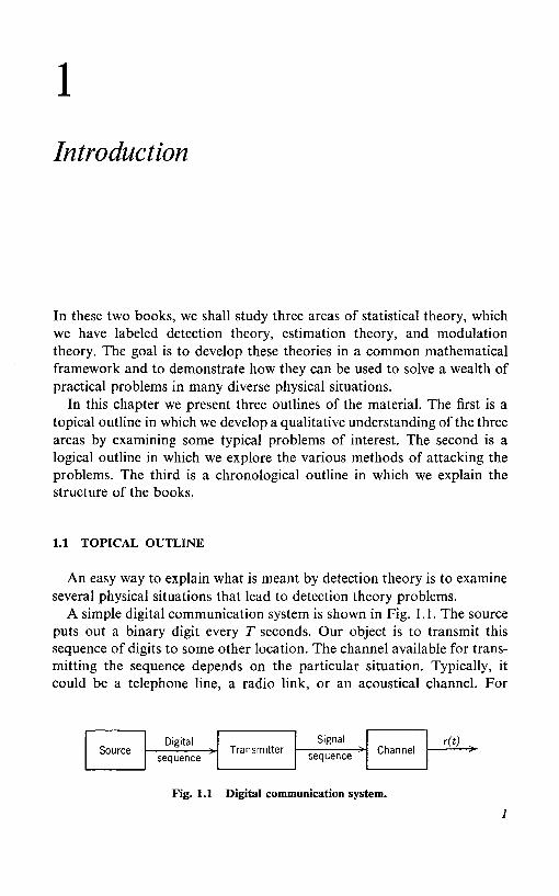
A simple digital communication system is shown in Fig. 1.1. The sourceputs out a binary digit every T seconds. Our object is to transmit thissequence of digits to some other location. The channel available for trans-mitting the sequence depends on the particular situation. Typically, itcould be a telephone line, a radio link, or an acoustical channel. For

Fig. 1.1 Digital communication system.

1

2 1.1 Topical Outline

purposes of illustration, we shall consider a radio link. In order to transmitthe information, we must put it into a form suitable for propagating overthe channel. A straightforward method would be to build a device thatgenerates a sine wave,

for T seconds if the source generated a "one" in the preceding interval,and a sine wave of a different frequency,

for T seconds if the source generated a "zero" in the preceding interval.The frequencies are chosen so that the signals J0(0 and s-^t) will propagateover the particular radio link of concern. The output of the device is fedinto an antenna and transmitted over the channel. Typical source andtransmitted signal sequences are shown in Fig. 1.2. In the simplest kind ofchannel the signal sequence arrives at the receiving antenna attenuated butessentially undistorted. To process the received signal we pass it throughthe antenna and some stages of rf-amplification, in the course of which athermal noise n(t) is added to the message sequence. Thus in any J-secondinterval we have available a waveform r(t) in which

if Si(t) was transmitted, and

if s0(t) was transmitted. We are now faced with the problem of decidingwhich of the two possible signals was transmitted. We label the device thatdoes this a decision device. It is simply a processor that observes r(t) andguesses whether S]_(t) or s0(t) was sent according to some set of rules. Thisis equivalent to guessing what the source output was in the precedinginterval. We refer to designing and evaluating the processor as a detection

Fig. 1.2 Typical sequences.

Detection Theory 3

Fig. 1.3 Sequence with phase shifts.

theory problem. In this particular case the only possible source of error inmaking a decision is the additive noise. If it were not present, the inputwould be completely known and we could make decisions without errors.We denote this type of problem as the known signal in noise problem. Itcorresponds to the lowest level (i.e., simplest) of the detection problems ofinterest.

An example of the next level of detection problem is shown in Fig. 1.3.The oscillators used to generate Si(t) and J0(0 in the preceding examplehave a phase drift. Therefore in a particular T-second interval the receivedsignal corresponding to a "one" is

and the received signal corresponding to a "zero" is

where 00 and dl are unknown constant phase angles. Thus even in theabsence of noise the input waveform is not completely known. In a practicalsystem the receiver may include auxiliary equipment to measure the oscilla-tor phase. If the phase varies slowly enough, we shall see that essentiallyperfect measurement is possible. If this is true, the problem is the same asabove. However, if the measurement is not perfect, we must incorporatethe signal uncertainty in our model.

A corresponding problem arises in the radar and sonar areas. A con-ventional radar transmits a pulse at some frequency o>c with a rectangularenvelope:

If a target is present, the pulse is reflected. Even the simplest target willintroduce an attenuation and phase shift in the transmitted signal. Thusthe signal available for processing in the interval of interest is

4 1.1 Topical Outline

if a target is present and

if a target is absent. We see that in the absence of noise the signal stillcontains three unknown quantities: Vr, the amplitude, 6r, the phase, andT, the round-trip travel time to the target.

These two examples represent the second level of detection problems.We classify them as signal with unknown parameters in noise problems.

Detection problems of a third level appear in several areas. In a passivesonar detection system the receiver listens for noise generated by enemyvessels. The engines, propellers, and other elements in the vessel generateacoustical signals that travel through the ocean to the hydrophones in thedetection system. This composite signal can best be characterized as asample function from a random process. In addition, the hydrophonegenerates self-noise and picks up sea noise. Thus a suitable model for thedetection problem might be

if the target is present and

if it is not. In the absence of noise the signal is a sample function from arandom process (indicated by the subscript Q).

In the communications field a large number of systems employ channelsin which randomness is inherent. Typical systems are tropospheric scatterlinks, orbiting dipole links, and chaff systems. A common technique is totransmit one of two signals separated in frequency. (We denote thesefrequencies as o^ and o>0.) The resulting received signal is

if Si(t) was transmitted and

if s0(t) was transmitted. Here sni(t) is a sample function from a randomprocess centered at o^, and sno(t) is a sample function from a randomprocess centered at a>0. These examples are characterized by the lack of anydeterministic signal component. Any decision procedure that we designwill have to be based on the difference in the statistical properties of thetwo random processes from which sno(t) and sni(t) are obtained. This isthe third level of detection problem and is referred to as a random signalin noise problem.

Estimation Theory 5

In our examination of representative examples we have seen that detec-tion theory problems are characterized by the fact that we must decidewhich of several alternatives is true. There were only two alternatives inthe examples cited; therefore we refer to them as binary detection prob-lems. Later we will encounter problems in which there are M alternativesavailable (the M-ary detection problem). Our hierarchy of detectionproblems is presented graphically in Fig. 1.4.

There is a parallel set of problems in the estimation theory area. Asimple example is given in Fig. 1.5, in which the source puts out ananalog message a(t) (Fig. l.5a). To transmit the message we first sample itevery T seconds. Then, every T seconds we transmit a signal that contains

Level 1. Known signals innoise

Level 2. Signals with unknownparameters in noise

Level 3. Random signals innoise

Detection theory

1. Synchronous digital communication

2. Pattern recognition problems

1. Conventional pulsed radar or sonar,target detection

2. Target classification (orientation oftarget unknown)

3. Digital communication systems withoutphase reference

4. Digital communication over slowly-fading channels

1. Digital communication over scatterlink, orbiting dipole channel, orchaff link

2. Passive sonar

3. Seismic detection system

4. Radio astronomy (detection of noisesources )

Fig. 1.4 Detection theory hierarchy.

6 1.1 Topical Outline

Fig. 1.5 (a) Sampling an analog source; (b) pulse-amplitude modulation; (c) pulse-frequency modulation; (</) waveform reconstruction.

a parameter which is uniquely related to the last sample value. In Fig. 1.56the signal is a sinusoid whose amplitude depends on the last sample. Thus,if the sample at time nT is An, the signal in the interval [nT, (n + l)T] is

A system of this type is called a pulse amplitude modulation (PAM)system. In Fig. 1.5c the signal is a sinusoid whose frequency in the interval

Estimation Theory 7

differs from the reference frequency a>c by an amount proportional to thepreceding sample value,

A system of this type is called a pulse frequency modulation (PFM) system.Once again there is additive noise. The received waveform, given that An

was the sample value, is

During each interval the receiver tries to estimate An. We denote theseestimates as An. Over a period of time we obtain a sequence of estimates,as shown in Fig. \.5d, which is passed into a device whose output is anestimate of the original message a(t). If a(t) is a band-limited signal, thedevice is just an ideal low-pass filter. For other cases it is more involved.

If, however, the parameters in this example were known and the noisewere absent, the received signal would be completely known. We referto problems in this category as known signal in noise problems. If weassume that the mapping from An to s(t, An) in the transmitter has aninverse, we see that if the noise were not present we could determine An

unambiguously. (Clearly, if we were allowed to design the transmitter, weshould always choose a mapping with an inverse.) The known signal innoise problem is the first level of the estimation problem hierarchy.

Returning to the area of radar, we consider a somewhat differentproblem. We assume that we know a target is present but do not knowits range or velocity. Then the received signal is

where a>d denotes a Doppler shift caused by the target's motion. We wantto estimate r and <od. Now, even if the noise were absent and r and o>d

were known, the signal would still contain the unknown parameters Vr

and 6r. This is a typical second-level estimation problem. As in detectiontheory, we refer to problems in this category as signal with unknownparameters in noise problems.

At the third level the signal component is a random process whosestatistical characteristics contain parameters we want to estimate. Thereceived signal is of the form

where sn(t, A) is a sample function from a random process. In a simplecase it might be a stationary process with the narrow-band spectrum shownin Fig. 1.6. The shape of the spectrum is known but the center frequency

Fig. 1.6 Spectrum of random signal.

Level 1. Known signals in noise

Level 2. Signals with unknownparameters in noise

Level 3. Random signals in noise

Estimation Theory

1. RAM, PFM, and PPM communication systemswith phase synchronization

2. Inaccuracies in inertial systems(e.g., drift angle measurement)

1. Range, velocity, or angle measurement inradar/sonar problems

2. Discrete time, continuous amplitude communicationsystem (with unknown amplitude or phase inchannel)

1. Power spectrum parameter estimation

2. Range or Doppler spread target parametersin radar/sonar problem

3. Velocity measurement in radio astronomy

4. Target parameter estimation: passive sonar

5. Ground mapping radars

Fig. 1.7 Estimation theory hierarchy.

8

Modulation Theory 9

is not. The receiver must observe r(t) and, using the statistical propertiesof sn(t, A) and n(t), estimate the value of A. This particular example couldarise in either radio astronomy or passive sonar. The general class ofproblem in which the signal containing the parameters is a sample functionfrom a random process is referred to as the random signal in noise problem.The hierarchy of estimation theory problems is shown in Fig. 1.7.

We note that there appears to be considerable parallelism in the detectionand estimation theory problems. We shall frequently exploit these parallelsto reduce the work, but there is a basic difference that should be em-phasized. In binary detection the receiver is either "right" or "wrong."In the estimation of a continuous parameter the receiver will seldom beexactly right, but it can try to be close most of the time. This differencewill be reflected in the manner in which we judge system performance.

The third area of interest is frequently referred to as modulation theory.We shall see shortly that this term is too narrow for the actual problems.Once again a simple example is useful. In Fig. 1.8 we show an analogmessage source whose output might typically be music or speech. Toconvey the message over the channel, we transform it by using a modula-tion scheme to get it into a form suitable for propagation. The transmittedsignal is a continuous waveform that depends on a(t) in some deterministicmanner. In Fig. 1.8 it is an amplitude modulated waveform:

(This is conventional double-sideband AM with modulation index m.) InFig. 1.8c the transmitted signal is a frequency modulated (FM) waveform:

When noise is added the received signal is

Now the receiver must observe r(t) and put out a continuous estimate ofthe message a(t), as shown in Fig. 1.8. This particular example is a first-level modulation problem, for if n(t) were absent and a(t) were known thereceived signal would be completely known. Once again we describe it asa known signal in noise problem.

Another type of physical situation in which we want to estimate acontinuous function is shown in Fig. 1.9. The channel is a time-invariantlinear system whose impulse response h(r) is unknown. To estimate theimpulse response we transmit a known signal x(t). The received signal is

Fig. 1.8 A modulation theory example: (a) analog transmission system; (b) amplitudemodulated signal; (c) frequency modulated signal; (</) demodulator.

Fig. 1.9 Channel measurement.

10

Modulation Theory 11

The receiver observes r(t) and tries to estimate /J(T). This particular examplecould best be described as a continuous estimation problem. Many otherproblems of interest in which we shall try to estimate a continuous wave-form will be encountered. For convenience, we shall use the term modula-tion theory for this category, even though the term continuous waveformestimation might be more descriptive.

The other levels of the modulation theory problem follow by directanalogy. In the amplitude modulation system shown in Fig. \.%b thereceiver frequently does not know the phase angle of the carrier. In thiscase a suitable model is

1. Known signals in noise

2. Signals with unknownparameters in noise

3. Random signals in noise

Modulation Theory (Continuous waveform estimation)

1. Conventional communication systemssuch as AM (DSB-AM, SSB), FM.andPM with phase synchronization

2. Optimum filter theory

3. Optimum feedback systems

4. Channel measurement

5. Orbital estimation for satellites

6. Signal estimation in seismic andsonar classification systems

7. Synchronization in digital systems

1. Conventional communication systemswithout phase synchronization

2. Estimation of channel characteristics whenphase of input signal is unknown

1. Analog communication overrandomly varying channels

2. Estimation of statistics oftime-varying processes

3. Estimation of plant characteristics

Fig. 1.10 Modulation theory hierarchy.

12 1.2 Possible Approaches

where 6 is an unknown parameter. This is an example of a signal withunknown parameter problem in the modulation theory area.

A simple example of a third-level problem (random signal in noise} is onein which we transmit a frequency-modulated signal over a radio link whosegain and phase characteristics are time-varying. We shall find that if wetransmit the signal in (20) over this channel the received waveform will be

where V(t) and 0(t) are sample functions from random processes. Thus,even if a(u) were known and the noise n(t} were absent, the received signalwould still be a random process. An over-all outline of the problems ofinterest to us appears in Fig. 1.10. Additional examples included in thetable to indicate the breadth of the problems that fit into the outline arediscussed in more detail in the text.

Now that we have outlined the areas of interest it is appropriate todetermine how to go about solving them.

1.2 POSSIBLE APPROACHES

From the examples we have discussed it is obvious that an inherentfeature of all the problems is randomness of source, channel, or noise(often all three). Thus our approach must be statistical in nature. Evenassuming that we are using a statistical model, there are many differentways to approach the problem. We can divide the possible approaches intotwo categories, which we denote as "structured" and "nonstructured."Some simple examples will illustrate what we mean by a structuredapproach.

Example 1. The input to a linear time-invariant system is r(t):

The impulse response of the system is h(r). The signal s(t) is a known function withenergy Es,

and w(t) is a sample function from a zero-mean random process with a covariancefunction:

We are concerned with the output of the system at time T. The output due to thesignal is a deterministic quantity:

Structured Approach 13

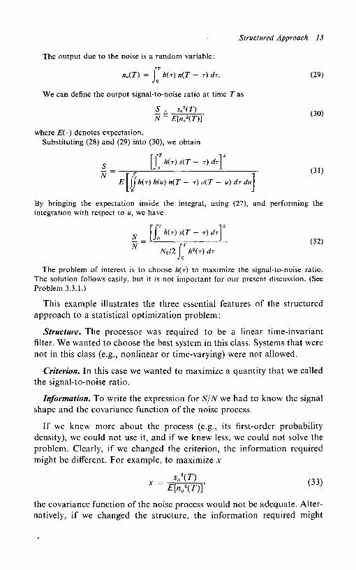
The output due to the noise is a random variable:

We can define the output signal-to-noise ratio at time T as

where £"(•) denotes expectation.Substituting (28) and (29) into (30), we obtain

By bringing the expectation inside the integral, using (27), and performing theintegration with respect to u, we have

The problem of interest is to choose h(r) to maximize the signal-to-noise ratio.The solution follows easily, but it is not important for our present discussion. (SeeProblem 3.3.1.)

This example illustrates the three essential features of the structuredapproach to a statistical optimization problem:

Structure. The processor was required to be a linear time-invariantfilter. We wanted to choose the best system in this class. Systems that werenot in this class (e.g., nonlinear or time-varying) were not allowed.

Criterion. In this case we wanted to maximize a quantity that we calledthe signal-to-noise ratio.

Information. To write the expression for S/N we had to know the signalshape and the covariance function of the noise process.

If we knew more about the process (e.g., its first-order probabilitydensity), we could not use it, and if we knew less, we could not solve theproblem. Clearly, if we changed the criterion, the information requiredmight be different. For example, to maximize x

the covariance function of the noise process would not be adequate. Alter-natively, if we changed the structure, the information required might