detection and estimation of signals in noise and estimation of signals in noise ... signal detection...

Detection and Estimation of Signalsin Noise

Dr. Robert SchoberDepartment of Electrical and Computer Engineering

University of British Columbia

Vancouver, August 24, 2010

2

Contents

1 Basic Elements of a Digital CommunicationSystem 1

1.1 Transmitter . . . . . . . . . . . . . . . . . . . . . . . . . . . . . . . . . . . . . . 1

1.2 Receiver . . . . . . . . . . . . . . . . . . . . . . . . . . . . . . . . . . . . . . . . 3

1.3 Communication Channels . . . . . . . . . . . . . . . . . . . . . . . . . . . . . . 4

1.3.1 Physical Channel . . . . . . . . . . . . . . . . . . . . . . . . . . . . . . . 4

1.3.2 Mathematical Models for Communication Channels . . . . . . . . . . . . 5

2 Probability and Stochastic Processes 9

2.1 Probability . . . . . . . . . . . . . . . . . . . . . . . . . . . . . . . . . . . . . . 9

2.1.1 Basic Concepts . . . . . . . . . . . . . . . . . . . . . . . . . . . . . . . . 9

2.1.2 Random Variables . . . . . . . . . . . . . . . . . . . . . . . . . . . . . . 14

2.1.3 Functions of Random Variables . . . . . . . . . . . . . . . . . . . . . . . 21

2.1.4 Statistical Averages of RVs . . . . . . . . . . . . . . . . . . . . . . . . . . 26

2.1.5 Gaussian Distribution . . . . . . . . . . . . . . . . . . . . . . . . . . . . 31

2.1.6 Chernoff Upper Bound on the Tail Probability . . . . . . . . . . . . . . . 39

2.1.7 Central Limit Theorem . . . . . . . . . . . . . . . . . . . . . . . . . . . . 41

2.2 Stochastic Processes . . . . . . . . . . . . . . . . . . . . . . . . . . . . . . . . . 42

2.2.1 Statistical Averages . . . . . . . . . . . . . . . . . . . . . . . . . . . . . . 43

2.2.2 Power Density Spectrum . . . . . . . . . . . . . . . . . . . . . . . . . . . 50

2.2.3 Response of a Linear Time–Invariant System to a Random Input Signal . 52

2.2.4 Sampling Theorem for Band–Limited Stochastic Processes . . . . . . . . 56

2.2.5 Discrete–Time Stochastic Signals and Systems . . . . . . . . . . . . . . . 57

2.2.6 Cyclostationary Stochastic Processes . . . . . . . . . . . . . . . . . . . . 60

3 Characterization of Communication Signals and Systems 63

3.1 Representation of Bandpass Signals and Systems . . . . . . . . . . . . . . . . . . 63

3.1.1 Equivalent Complex Baseband Representation of Bandpass Signals . . . 64

3.1.2 Equivalent Complex Baseband Representation of Bandpass Systems . . . 74

3.1.3 Response of a Bandpass Systems to a Bandpass Signal . . . . . . . . . . 76

Schober: Signal Detection and Estimation

3

3.1.4 Equivalent Baseband Representation of Bandpass Stationary StochasticProcesses . . . . . . . . . . . . . . . . . . . . . . . . . . . . . . . . . . . 77

3.2 Signal Space Representation of Signals . . . . . . . . . . . . . . . . . . . . . . . 85

3.2.1 Vector Space Concepts – A Brief Review . . . . . . . . . . . . . . . . . . 85

3.2.2 Signal Space Concepts . . . . . . . . . . . . . . . . . . . . . . . . . . . . 88

3.2.3 Orthogonal Expansion of Signals . . . . . . . . . . . . . . . . . . . . . . 90

3.3 Representation of Digitally Modulated Signals . . . . . . . . . . . . . . . . . . . 103

3.3.1 Memoryless Modulation . . . . . . . . . . . . . . . . . . . . . . . . . . . 104

3.3.1.1 M-ary Pulse–Amplitude Modulation (MPAM) . . . . . . . . . 104

3.3.1.2 M-ary Phase–Shift Keying (MPSK) . . . . . . . . . . . . . . . 109

3.3.1.3 M-ary Quadrature Amplitude Modulation (MQAM) . . . . . . 112

3.3.1.4 Multi–Dimensional Modulation . . . . . . . . . . . . . . . . . . 115

3.3.1.5 M-ary Frequency–Shift Keying (MFSK) . . . . . . . . . . . . . 116

3.3.2 Linear Modulation With Memory . . . . . . . . . . . . . . . . . . . . . . 122

3.3.2.1 M–ary Differential Phase–Shift Keying (MDPSK) . . . . . . . 122

3.3.3 Nonlinear Modulation With Memory . . . . . . . . . . . . . . . . . . . . 124

3.3.3.1 Continuous–Phase FSK (CPFSK) . . . . . . . . . . . . . . . . . 124

3.3.3.2 Continuous Phase Modulation (CPM) . . . . . . . . . . . . . . 128

3.4 Spectral Characteristics of Digitally Modulated Signals . . . . . . . . . . . . . . 141

3.4.1 Linearly Modulated Signals . . . . . . . . . . . . . . . . . . . . . . . . . 141

3.4.2 CPFSK and CPM . . . . . . . . . . . . . . . . . . . . . . . . . . . . . . 150

4 Optimum Reception in Additive White Gaussian Noise (AWGN) 151

4.1 Optimum Receivers for Signals Corrupted by AWGN . . . . . . . . . . . . . . . 151

4.1.1 Demodulation . . . . . . . . . . . . . . . . . . . . . . . . . . . . . . . . . 153

4.1.1.1 Correlation Demodulation . . . . . . . . . . . . . . . . . . . . . 153

4.1.1.2 Matched–Filter Demodulation . . . . . . . . . . . . . . . . . . . 158

4.1.2 Optimal Detection . . . . . . . . . . . . . . . . . . . . . . . . . . . . . . 164

4.2 Performance of Optimum Receivers . . . . . . . . . . . . . . . . . . . . . . . . . 174

4.2.1 Binary Modulation . . . . . . . . . . . . . . . . . . . . . . . . . . . . . . 174

4.2.2 M–ary PAM . . . . . . . . . . . . . . . . . . . . . . . . . . . . . . . . . . 182

4.2.3 M–ary PSK . . . . . . . . . . . . . . . . . . . . . . . . . . . . . . . . . . 186


4

4.2.4 M–ary QAM . . . . . . . . . . . . . . . . . . . . . . . . . . . . . . . . . 187

4.2.5 Upper Bound for Arbitrary Linear Modulation Schemes . . . . . . . . . . 188

4.2.6 Comparison of Different Linear Modulations . . . . . . . . . . . . . . . . 190

4.3 Receivers for Signals with Random Phase in AWGN . . . . . . . . . . . . . . . . 192

4.3.1 Channel Model . . . . . . . . . . . . . . . . . . . . . . . . . . . . . . . . 192

4.3.2 Noncoherent Detectors . . . . . . . . . . . . . . . . . . . . . . . . . . . . 194

4.3.2.1 A Simple Noncoherent Detector for PSK with Differential En-coding (DPSK) . . . . . . . . . . . . . . . . . . . . . . . . . . . 195

4.3.2.2 Optimum Noncoherent Detection . . . . . . . . . . . . . . . . . 201

4.3.2.3 Optimum Noncoherent Detection of Binary Orthogonal Modu-lation . . . . . . . . . . . . . . . . . . . . . . . . . . . . . . . . 205

4.3.2.4 Optimum Noncoherent Detection of On–Off Keying . . . . . . . 210

4.3.2.5 Multiple–Symbol Differential Detection (MSDD) of DPSK . . . 212

4.4 Optimum Coherent Detection of Continuous Phase Modulation (CPM) . . . . . 218

5 Signal Design for Bandlimited Channels 225

5.1 Characterization of Bandlimited Channels . . . . . . . . . . . . . . . . . . . . . 226

5.2 Signal Design for Bandlimited Channels . . . . . . . . . . . . . . . . . . . . . . 228

5.3 Discrete–Time Channel Model for ISI–free Transmission . . . . . . . . . . . . . 240

6 Equalization of Channels with ISI 244

6.1 Discrete–Time Channel Model . . . . . . . . . . . . . . . . . . . . . . . . . . . . 245

6.2 Maximum–Likelihood Sequence Estimation (MLSE) . . . . . . . . . . . . . . . . 247

6.3 Linear Equalization (LE) . . . . . . . . . . . . . . . . . . . . . . . . . . . . . . . 257

6.3.1 Optimum Linear Zero–Forcing (ZF) Equalization . . . . . . . . . . . . . 258

6.3.2 ZF Equalization with FIR Filters . . . . . . . . . . . . . . . . . . . . . . 263

6.3.3 Optimum Minimum Mean–Squared Error (MMSE) Equalization . . . . . 268

6.3.4 MMSE Equalization with FIR Filters . . . . . . . . . . . . . . . . . . . . 278

6.4 Decision–Feedback Equalization (DFE) . . . . . . . . . . . . . . . . . . . . . . . 283

6.4.1 Optimum ZF–DFE . . . . . . . . . . . . . . . . . . . . . . . . . . . . . . 288

6.4.2 Optimum MMSE–DFE . . . . . . . . . . . . . . . . . . . . . . . . . . . . 295

6.5 MMSE–DFE with FIR Filters . . . . . . . . . . . . . . . . . . . . . . . . . . . . 301


II

Course Outline

1. Basic Elements of a Digital Communication System

2. Probability and Stochastic Processes – a Brief Review

3. Characterization of Communication Signals and Systems

4. Detection of Signals in Additive White Gaussian Noise

5. Bandlimited Channels

6. Equalization


1

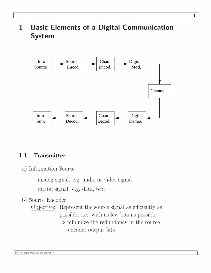
1 Basic Elements of a Digital Communication

System

InfoSource

InfoSink

SourceEncod.

DigitalMod.

DigitalDemod.

SourceDecod.

Channel

Chan.Encod.

Chan.Decod.

1.1 Transmitter

a) Information Source

– analog signal: e.g. audio or video signal

– digital signal: e.g. data, text

b) Source EncoderObjective: Represent the source signal as efficiently as

possible, i.e., with as few bits as possible

⇒ minimize the redundancy in the source

encoder output bits


2

c) Channel EncoderObjective: Increase reliability of received data

⇒ add redundancy in a controlled manner to

information bits

d) Digital Modulator

Objective: Transmit most efficiently over the

(physical) transmission channel

⇒ map the input bit sequence to a signal waveform

which is suitable for the transmission channel

Examples: Binary modulation:

bit 0 → s0(t)

bit 1 → s1(t)

⇒ 1 bit per channel use

M–ary modulation:

we map b bits to one waveform

⇒ we need M = 2b different waveforms to represent

all possible b–bit combinations

⇒ b bit/(channel use)


3

1.2 Receiver

a) Digital Demodulator

Objective: Reconstruct transmitted data symbols (binary or

M–ary from channel–corrupted received signal

b) Channel Decoder

Objective: Exploit redundancy introduced by channel encoder

to increase reliability of information bits

Note: In modern receivers demodulation and decoding is

sometimes performed in an iterative fashion.

c) Source Decoder

Objective: Reconstruct original information signal from

output of channel decoder


4

1.3 Communication Channels

1.3.1 Physical Channel

a) Types

– wireline

– optical fiber

– optical wireless channel

– wireless radio frequency (RF) channel

– underwater acoustic channel

– storage channel (CD, disc, etc.)

b) Impairments

– noise from electronic components in transmitter and receiver

– amplifier nonlinearities

– other users transmitting in same frequency band at the same

time (co–channel or multiuser interference)

– linear distortions because of bandlimited channel

– time–variance in wireless channels

For the design of the transmitter and the receiver we need a simple

mathematical model of the physical communication channel that

captures its most important properties. This model will vary from

one application to another.


5

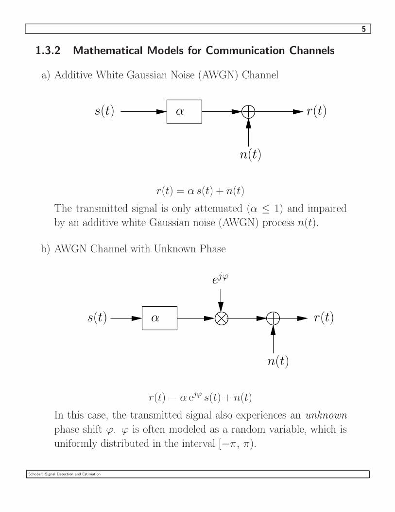
1.3.2 Mathematical Models for Communication Channels

a) Additive White Gaussian Noise (AWGN) Channel

n(t)

s(t) α r(t)

r(t) = α s(t) + n(t)

The transmitted signal is only attenuated (α ≤ 1) and impaired

by an additive white Gaussian noise (AWGN) process n(t).

b) AWGN Channel with Unknown Phase

s(t) α

ejϕ

n(t)

r(t)

r(t) = α ejϕ s(t) + n(t)

In this case, the transmitted signal also experiences an unknown

phase shift ϕ. ϕ is often modeled as a random variable, which is

uniformly distributed in the interval [−π, π).


6

c) Linearly Dispersive Channel (Linear Filter Channel)

n(t)

r(t)s(t) c(t)

c(t): channel impulse response; ∗: linear convolution

r(t) = c(t) ∗ s(t) + n(t)

=

∞∫

−∞

c(τ ) s(t − τ )dτ + n(t)

Transmit signal is linearly distorted by c(t) and impaired by AWGN.

d) Multiuser Channel

Two users:

s1(t)

s2(t)n(t)

r(t)

K–user channel:

r(t) =K∑

k=1

sk(t) + n(t)


7

e) Other Channels

– time–variant channels

– stochastic (random) channels

– fading channels

– multiple–input multiple–output (MIMO) channels

– . . .


8

Some questions that we want to answer in this course:

� Which waveforms are used for digital communications?

� How are these waveforms demodulate/detect?

� What performance (= bit or symbol error rate) can be achieved?


9

2 Probability and Stochastic Processes

Motivation:

� Very important mathematical tools for the design and analysis of

communication systems

� Examples:

– The transmitted symbols are unknown at the receiver and are

modeled as random variables.

– Impairments such as noise and interference are also unknown

at the receiver and are modeled as stochastic processes.

2.1 Probability

2.1.1 Basic Concepts

Given: Sample space S containing all possible outcomes of an exper-

iment

Definitions:

� Events A and B are subsets of S, i.e., A ⊆ S, B ⊆ S

� The complement of A is denoted by A and contains all elements

of S not included in A

� Union of two events: D = A∪B consists of all elements of A and

B

⇒ A ∪ A = S


10

� Intersection of two elements: E = A ∩B

Mutually exclusive events have as intersection the null element ◦/

e.g. A ∩ A = ◦/.

� Associated with each event A is its probability P (A)

Axioms of Probability

1. P (S) = 1 (certain event)

2. 0 ≤ P (A) ≤ 1

3. If A ∩ B = ◦/ then P (A ∪B) = P (A) + P (B)

The entire theory of probability is based on these three axioms.

E.g. it can be proved that

� P (A) = 1 − P (A)

� A ∩B 6= ◦/ then P (A ∪ B) = P (A) + P (B) − P (A ∩ B)

Example:

Fair die

– S = {1, 2, 3, 4, 5, 6}

– A = {1, 2, 5}, B = {3, 4, 5}

– A = {3, 4, 6}

– D = A ∪B = {1, 2, 3, 4, 5}

– E = A ∩B = {5}

– P (1) = P (2) = . . . = P (6) = 16


11

– P (A) = P (1) + P (2) + P (5) = 12, P (B) = 1

2

– P (D) = P (A) + P (B) − P (A ∩ B) = 12

+ 12−

16

= 56

Joint Events and Joint Probabilities

� Now we consider two experiments with outcomes

Ai, i = 1, 2, . . . n

and

Bj, j = 1, 2, . . .m

� We carry out both experiments and assign the outcome (Ai, Bj)

the probability P (Ai, Bj) with

0 ≤ P (Ai, Bj) ≤ 1

� If the outcomes Bj, j = 1, 2, . . . , m are mutually exclusive we

getm∑j=1

P (Ai, Bj) = P (Ai)

A similar relation holds if the outcomes of Ai, i = 1, 2, . . . n are

mutually exclusive.

� If all outcomes of both experiments are mutually exclusive, then

n∑i=1

m∑j=1

P (Ai, Bj) = 1


12

Conditional Probability

� Given: Joint event (A,B)

� Conditional probability P (A|B): Probability of event A given

that we have already observed event B

� Definition:

P (A|B) =P (A,B)

P (B)

(P (B) > 0 is assumed, for P (B) = 0 we cannot observe event B)

Similarly:

P (B|A) =P (A,B)

P (A)

� Bayes’ Theorem:

From

P (A, B) = P (A|B)P (B) = P (B|A)P (A)

we get

P (A|B) =P (B|A)P (A)

P (B)


13

Statistical Independence

If observing B does not change the probability of observing A, i.e.,

P (A|B) = P (A),

then A and B are statistically independent.

In this case:

P (A,B) = P (A|B)P (B)

= P (A)P (B)

Thus, two events A and B are statistically independent if and only if

P (A,B) = P (A)P (B)


14

2.1.2 Random Variables

� We define a functionX(s), where s ∈ S are elements of the sample

space.

� The domain of X(s) is S and its range is the set of real numbers.

� X(s) is called a random variable.

� X(s) can be continuous or discrete.

� We use often simply X instead of X(s) to denote the random

variable.

Example:

- Fair die: S = {1, 2, . . . , 6} and

X(s) =

{1, s ∈ {1, 3, 5}

0, s ∈ {2, 4, 6}

- Noise voltage at resistor: S is continuous (e.g. set of all real

numbers) and so is X(s) = s


15

Cumulative Distribution Function (CDF)

� Definition: F (x) = P (X ≤ x)

The CDF F (x) denotes the probability that the random variable

(RV) X is smaller than or equal to x.

� Properties:

0 ≤ F (x) ≤ 1

limx→−∞

F (x) = 0

limx→∞

F (x) = 1

d

dxF (x) ≥ 0

Example:

1. Fair die X = X(s) = s

1

21 3 4 5 6

1/6

x

F (x)

Note: X is a discrete random variable.


16

2. Continuous random variable

1

x

F (x)

Probability Density Function (PDF)

� Definition:

p(x) =dF (x)

dx, −∞ < x <∞

� Properties:

p(x) ≥ 0

F (x) =

x∫

−∞

p(u)du

∞∫

−∞

p(x)dx = 1


17

� Probability that x1 ≤ X ≤ x2

P (x1 ≤ X ≤ x2) =

x2∫

x1

p(x)dx = F (x2) − F (x1)

� Discrete random variables: X ∈ {x1, x2, . . . , xn}

p(x) =

n∑i=1

P (X = xi)δ(x− xi)

with the Dirac impulse δ(·)

Example:

Fair die

1 32 4 5 6

1/6

x

p(x)


18

Joint CDF and Joint PDF

� Given: Two random variables X , Y

� Joint CDF:

FXY (x, y) = P (X ≤ x, Y ≤ y)

=

x∫

−∞

y∫

−∞

pXY (u, v) du dv

where pXY (x, y, ) is the joint PDF of X and Y

� Joint PDF:

pXY (x, y) =∂2

∂x∂yFXY (x, y)

� Marginal densities

pX(x) =

∞∫

−∞

pXY (x, y) dy

pY (y) =

∞∫

−∞

pXY (x, y) dx


19

� Some properties of FXY (x, y) and pXY (x, y)

FXY (−∞,−∞) = FXY (x,−∞) = FXY (−∞, y) = 0

FXY (∞,∞) =

∞∫

−∞

∞∫

−∞

pXY (x, y) dx dy = 1

� Generalization to n random variables X1, X2, . . . , Xn: see text-

book

Conditional CDF and Conditional PDF

� Conditional PDF

pX|Y (x|y) =pXY (x, y)

pY (y)

� Conditional CDF

FX|Y (x|y) =

x∫

−∞

pX|Y (u|y) du

=

x∫−∞

pXY (u, y) du

pY (y)


20

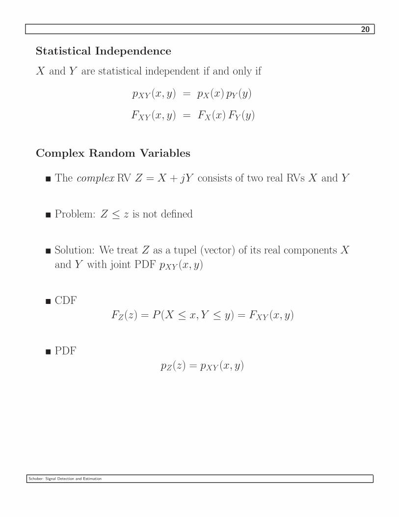
Statistical Independence

X and Y are statistical independent if and only if

pXY (x, y) = pX(x) pY (y)

FXY (x, y) = FX(x)FY (y)

Complex Random Variables

� The complex RV Z = X + jY consists of two real RVs X and Y

� Problem: Z ≤ z is not defined

� Solution: We treat Z as a tupel (vector) of its real components X

and Y with joint PDF pXY (x, y)

� CDF

FZ(z) = P (X ≤ x, Y ≤ y) = FXY (x, y)

� PDF

pZ(z) = pXY (x, y)


21

2.1.3 Functions of Random Variables

Problem Statement (one–dimensional case)

� Given:

– RV X with pX(x) and FX(x)

– RV Y = g(X) with function g(·)

� Calculate: pY (y) and FY (y)

Y

X

g(X)

Since a general solution to the problem is very difficult, we consider

some important special cases.

Special Cases:

a) Linear transformation Y = aX + b, a > 0

– CDF

FY (y) = P (Y ≤ y) = P (aX + b ≤ y) = P

(X ≤

y − b

a

)

=

(y−b)/a∫

−∞

pX(x) dx

= FX

(y − b

a

)


22

– PDF

pY (y) =∂

∂yFY (y) =

∂

∂y

∂x

∂xFX(x)

∣∣∣∣∣x=(y−b)/a

=∂x

∂y

∣∣∣∣∣x=(y−b)/a

∂

∂xFX(x)

∣∣∣∣∣x=(y−b)/a

=1

apX

(y − b

a

)

b) g(x) = y has real roots x1, x2, . . . , xn

– PDF

pY (y) =n∑i=1

pX(xi)

|g′(xi)|

with g′(xi) = ddxg(x)

∣∣∣∣∣x=xi

– CDF: Can be obtained from PDF by integration.

Example:

Y = aX2 + b, a > 0


23

Roots:

ax2 + b = y ⇒ x1/2 = ±

√y − b

a

g′(xi):d

dxg(x) = 2ax

PDF:

pY (y) =

pX

(√y−b

a

)

2a√

y−ba

+

pX

(−

√y−b

a

)

2a√

y−ba

c) A simple multi–dimensional case

– Given:

∗ RVs Xi, 1 ≤ i ≤ n with joint PDF pX(x1, x2, . . . , xn)

∗ Transformation: Yi = gi(x1, x2, . . . , xn), 1 ≤ i ≤ n

– Problem: Calculate pY (y1, y2, . . . , yn)

– Simplifying assumptions for gi(x1, x2, . . . , xn), 1 ≤ i ≤ n

∗ gi(x1, x2, . . . , xn), 1 ≤ i ≤ n, have continuous partial

derivatives


24

∗ gi(x1, x2, . . . , xn), 1 ≤ i ≤ n, are invertible, i.e.,

Xi = g−1i (Y1, Y2, . . . , Yn), 1 ≤ i ≤ n

– PDF:

pY (y1, y2, . . . , yn) = pX(x1 = g−11 , . . . , xn = g−1

n ) · |J |

with

∗ g−1i = g−1

i (y1, y2, . . . , yn)

∗ Jacobian of transformation

J =

∂(g−11 )

∂y1· · ·

∂(g−1n )

∂y1... ...∂(g−1

1 )∂yn

· · ·∂(g−1

n )∂yn

∗ |J |: Determinant of matrix J

d) Sum of two RVs X1 and X2

Y = X1 +X2

– Given: pX1X2(x1, x2)

– Problem: Find pY (y)


25

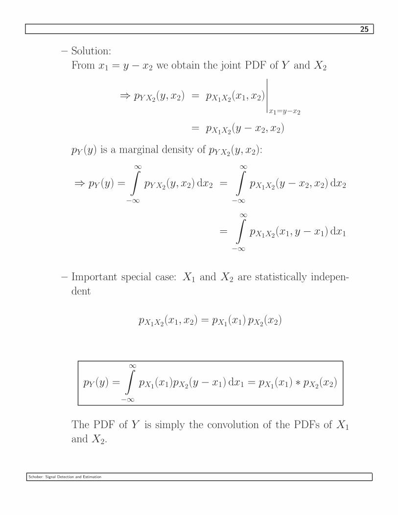
– Solution:

From x1 = y − x2 we obtain the joint PDF of Y and X2

⇒ pY X2(y, x2) = pX1X2

(x1, x2)

∣∣∣∣∣x1=y−x2

= pX1X2(y − x2, x2)

pY (y) is a marginal density of pY X2(y, x2):

⇒ pY (y) =

∞∫

−∞

pYX2(y, x2) dx2 =

∞∫

−∞

pX1X2(y − x2, x2) dx2

=

∞∫

−∞

pX1X2(x1, y − x1) dx1

– Important special case: X1 and X2 are statistically indepen-

dent

pX1X2(x1, x2) = pX1

(x1) pX2(x2)

pY (y) =

∞∫

−∞

pX1(x1)pX2

(y − x1) dx1 = pX1(x1) ∗ pX2

(x2)

The PDF of Y is simply the convolution of the PDFs of X1

and X2.


26

2.1.4 Statistical Averages of RVs

� Important for characterization of random variables.

General Case

� Given:

– RV Y = g(X) with random vector X = (X1, X2, . . . , Xn)

– (Joint) PDF pX(x) of X

� Expected value of Y :

E{Y } = E{g(X)} =

∞∫

−∞

· · ·

∞∫

−∞

g(x) pX(x) dx1 . . . dxn

E{·} denotes statistical averaging.

Special Cases (one–dimensional): X = X1 = X

� Mean: g(X) = X

mX = E{X} =

∞∫

−∞

x pX(x) dx

� nth moment: g(X) = Xn

E{Xn} =

∞∫

−∞

xn pX(x) dx


27

� nth central moment: g(X) = (X −mX)n

E{(X −mX)n} =

∞∫

−∞

(x−mX)n pX(x) dx

� Variance: 2nd central moment

σ2X =

∞∫

−∞

(x−mX)2 pX(x) dx

=

∞∫

−∞

x2 pX(x) dx +

∞∫

−∞

m2X pX(x) dx− 2

∞∫

−∞

mX x pX(x) dx

=

∞∫

−∞

x2 pX(x) dx−m2X

= E{X2} − (E{X})2

Complex case: σ2X = E{|X|2} − |E{X}|2

� Characteristic function: g(X) = ejvX

ψ(jv) = E{ejvX} =

∞∫

−∞

ejvx pX(x) dx


28

Some properties of ψ(jv):

– ψ(jv) = G(−jv), whereG(jv) denotes the Fourier transform

of pX(x)

– pX(x) =1

2π

∞∫

−∞

ψ(jv) e−jvX dv

– E{Xn} = (−j)ndn ψ(jv)

dvn

∣∣∣∣∣v=0

Given ψ(jv) we can easily calculate the nth moment of X .

– Application: Calculation of PDF of sum Y = X1 + X2 of

statistically independent RVs X1 and X2

∗ Given: pX1(x1), pX2

(x2) or equivalently ψX1(jv), ψX2

(jv)

∗ Problem: Find pY (y) or equivalently ψY (jv)

∗ Solution:

ψY (jv) = E{ejvY }

= E{ejv(X1+X2)}

= E{ejvX1} E{ejvX2}

= ψX1(jv)ψX2

(jv)

ψY (jv) is simply product of ψX1(jv) and ψX2

(jv). This

result is not surprising since pY (y) is the convolution of

pX1(x1) and pX1

(x2) (see Section 2.1.3).


29

Special Cases (multi–dimensional)

� Joint higher order moments g(X1, X2) = Xk1X

n2

E{Xk1X

n2 } =

∞∫

−∞

∞∫

−∞

xk1 xn2 pX1X2

(x1, x2) dx1 dx2

Special case k = n = 1: ρX1X2= E{X1X2} is called the correla-

tion between X1 and X2.

� Covariance (complex case): g(X1, X2) = (X1−mX1)(X2−mX2

)∗

µX1X2= E{(X1 −mX1

)(X2 −mX2)∗}

=

∞∫

−∞

∞∫

−∞

(x1 −mX1) (x2 −mX2

)∗ pX1X2(x1, x2) dx1 dx2

= E{X1X∗2} − E{X1} E{X

∗2}

mX1and mX2

denote the means of X1 and X2, respectively.

X1 and X2 are uncorrelated if µX1X2= 0 is valid.

� Autocorrelation matrix of random vector X = (X1, X2, . . . , Xn)T

R = E{X XH}

H is the Hermitian operator and means transposition and conju-

gation.


30

� Covariance matrix

M = E{(X − mX) (X − mX)H}

= R − mXmHX

with mean vector mX = E{X}

� Characteristic function (two–dimensional case): g(X1, X2) = ej(v1X1+v2X2)

ψ(jv1, jv2) =

∞∫

−∞

∞∫

−∞

ej(v1x1+v2x2) pX1X2(x1, x2) dx1 dx2

ψ(jv1, jv2) can be applied to calculate the joint (higher order)

moments of X1 and X2.

E.g. E{X1X2} = −∂2ψ(jv1, jv2)

∂v1∂v2

∣∣∣∣∣v1=v2=0


31

2.1.5 Gaussian Distribution

The Gaussian distribution is the most important probability distribu-

tion in practice:

� Many physical phenomena can be described by a Gaussian distri-

bution.

� Often we also assume that a certain RV has a Gaussian distribu-

tion in order to render a problem mathematical tractable.

Real One–dimensional Case

� PDF of Gaussian RV X with mean mX and variance σ2

p(x) =1

√2πσ

e−(x−mX )2/(2σ2)

Note: The Gaussian PDF is fully characterized by its first and

second order moments!

� CDF

F (x) =

x∫

−∞

p(u) du =1

√2πσ

x∫

−∞

e−(u−mX)2/(2σ2) du

=1

2

2√π

x−mX√2σ∫

−∞

e−t2

dt =1

2+

1

2erf

(x−mX√

2σ

)


32

with the error function

erf(x) =2√π

x∫

0

e−t2

dt

Alternatively, we can express the CDF of a Gaussian RV in terms

of the complementary error function:

F (x) = 1 −1

2erfc

(x−mX√

2σ

)

with

erfc(x) =2√π

∞∫

x

e−t2

dt

= 1 − erf(x)

� Gaussian Q–function

The integral over the tail [x, ∞) of a normal distribution (= Gaus-

sian distribution with mX = 0, σ2 = 1) is referred to as the Gaus-

sian Q–function:

Q(x) =1

√2π

∞∫

x

e−t2/2 dt

The Q–function often appears in analytical expressions for error

probabilities for detection in AWGN.

The Q–function can be also expressed as

Q(x) =1

2erfc

(x√

2

)


33

Sometimes it is also useful to express the Q–function as

Q(x) =1

π

π/2∫

0

exp

(−

x2

2sin2Θ

)dΘ.

The main advantage of this representation is that the integral has

finite limits and does not depend on x. This is sometimes useful

in error rate analysis, especially for fading channels.

� Characteristic function

ψ(jv) =

∞∫

−∞

ejvx p(x) dx

=

∞∫

−∞

ejvx[

1√

2πσe(x−mX)2/(2σ2)

]dx

= ejvmX−v2σ2/2

� Moments

Central moments:

E{(X −mX)k} = µk =

{1 · 3 · · · (k − 1)σk even k

0 odd k


34

Non–central moments

E{Xk} =

k∑i=0

(k

i

)miXµk−i

Note: All higher order moments of a Gaussian RV can be expressed

in terms of its first and second order moments.

� Sum of n statistically independent RVs X1, X2, . . . , Xn

Y =n∑i=1

Xi

Xi has mean mi and variance σ2i .

Characteristic function:

ψY (jv) =n∏i=1

ψXi(jv)

=n∏i=1

ejvmi−v2σ2

i /2

= ejvmY −v2σ2Y/2

with

mY =

n∑i=1

mi

σ2Y =

n∑i=1

σ2i


35

⇒ The sum of statistically independent Gaussian RVs is also a

Gaussian RV. Note that the same statement is true for the sum of

statistical dependent Gaussian RVs.

Real Multi–dimensional (Multi–variate) Case

� Given:

– Vector X = (X1, X2, . . . , Xn)T of n Gaussian RVs

– Mean vector mX = E{X}

– Covariance matrix M = E{(X − mX)(X − mX)H}

� PDF

p(x) =1

(2π)n/2√

|M |exp

(−

1

2(x − mX)TM−1(x − mX)

)

� Special case: n = 2

mX =

[m1

m2

], M =

[σ2

1 µ12

µ12 σ22

]

with the joint central moment

µ12 = E{(X1 −m1)(X2 −m2)}

Using the normalized covariance ρ = µ12/(σ1σ2), 0 ≤ ρ ≤ 1, we


36

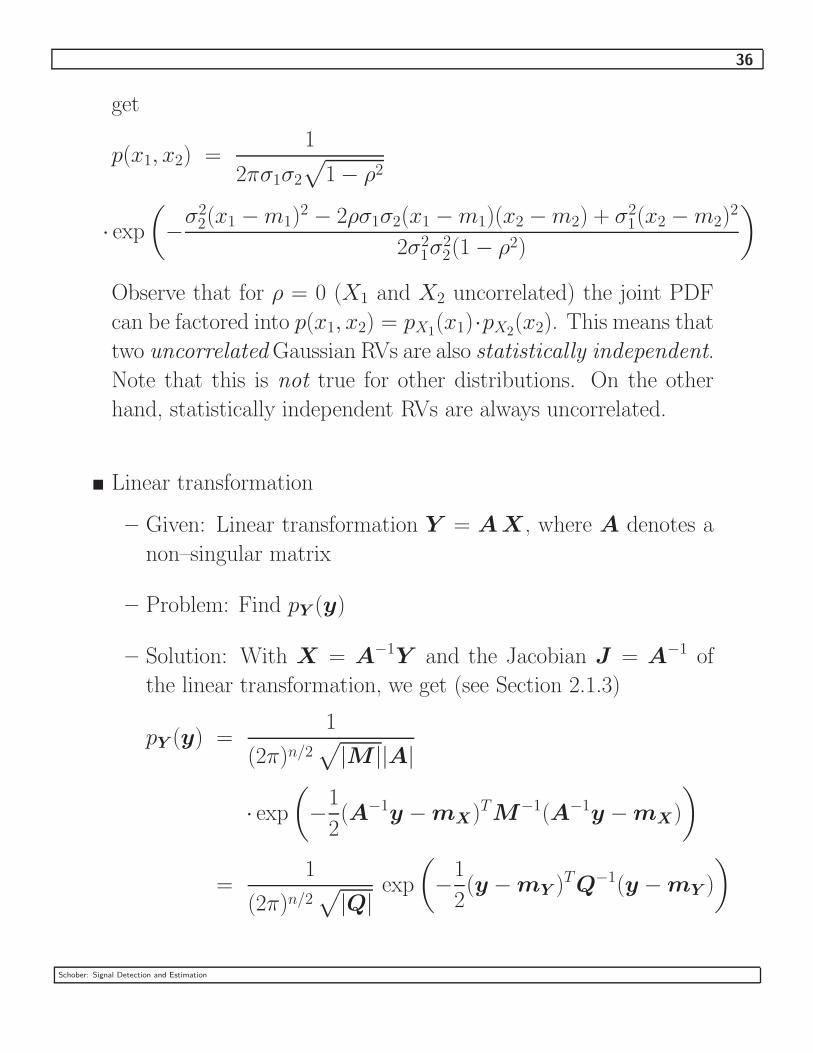
get

p(x1, x2) =1

2πσ1σ2

√1 − ρ2

· exp

(−σ2

2(x1 −m1)2 − 2ρσ1σ2(x1 −m1)(x2 −m2) + σ2

1(x2 −m2)2

2σ21σ

22(1 − ρ2)

)

Observe that for ρ = 0 (X1 and X2 uncorrelated) the joint PDF

can be factored into p(x1, x2) = pX1(x1)·pX2

(x2). This means that

two uncorrelated Gaussian RVs are also statistically independent.

Note that this is not true for other distributions. On the other

hand, statistically independent RVs are always uncorrelated.

� Linear transformation

– Given: Linear transformation Y = A X , where A denotes a

non–singular matrix

– Problem: Find pY (y)

– Solution: With X = A−1Y and the Jacobian J = A−1 of

the linear transformation, we get (see Section 2.1.3)

pY (y) =1

(2π)n/2√

|M ||A|

· exp

(−

1

2(A−1y − mX)TM−1(A−1y − mX)

)

=1

(2π)n/2√

|Q|exp

(−

1

2(y − mY )TQ−1(y − mY )

)


37

where vector mY and matrix Q are defined as

mY = A mX

Q = AMAT

We obtain the important result that a linear transformation of

a vector of jointly Gaussian RVs results in another vector of

jointly Gaussian RVs!

Complex One–dimensional Case

� Given: Z = X + jY , where X and Y are two Gaussian ran-

dom variables with means mX and mY , and variances σ2X and σ2

Y ,

respectively

� Most important case: X and Y are uncorrelated and σ2X = σ2

Y =

σ2 (in this case, Z is also referred to as a proper Gaussian RV)

� PDF

pZ(z) = pXY (x, y) = pX(x) pY (y)

=1

√2πσ

e−(x−mX )2/(2σ2)·

1√

2πσe−(y−mY )2/(2σ2)

=1

2πσ2e−((x−mX )2+(y−mY )2)/(2σ2)

=1

πσ2Z

e−|z−mZ |2/σ2

Z


38

with

mZ = E{Z} = mX + jmY

and

σ2Z = E{|Z −mZ|

2} = σ2

X + σ2Y = 2σ2

Complex Multi–dimensional Case

� Given: Complex vector Z = X + jY , where X and Y are two

real jointly Gaussian vectors with mean vectors mX and mY and

covariance matrices MX and MY , respectively

� Most important case: X and Y are uncorrelated and MX = MY

(proper complex random vector)

� PDF

pZ(z) =1

πn |MZ|exp

(−(z − mZ)HM−1

Z (z − mZ))

with

mZ = E{z} = mX + jmY

and

MZ = E{(z − mZ)(z − mZ)H} = MX + M Y


39

2.1.6 Chernoff Upper Bound on the Tail Probability

� The “tail probability” (area under the tail of PDF) often has to

be evaluated to determine the error probability of digital commu-

nication systems

� Closed–form results are often not feasible ⇒ the simple Chernoff

upper bound can be used for system design and/or analysis

� Chernoff Bound

The tail probability is given by

P (X ≥ δ) =

∞∫

δ

p(x) dx

=

∞∫

−∞

g(x) p(x) dx

= E{g(X)}

where we use the definition

g(X) =

{1, X ≥ δ

0, X < δ

.

Obviously g(X) can be upper bounded by g(X) ≤ eα(X−δ) with

α ≥ 0.


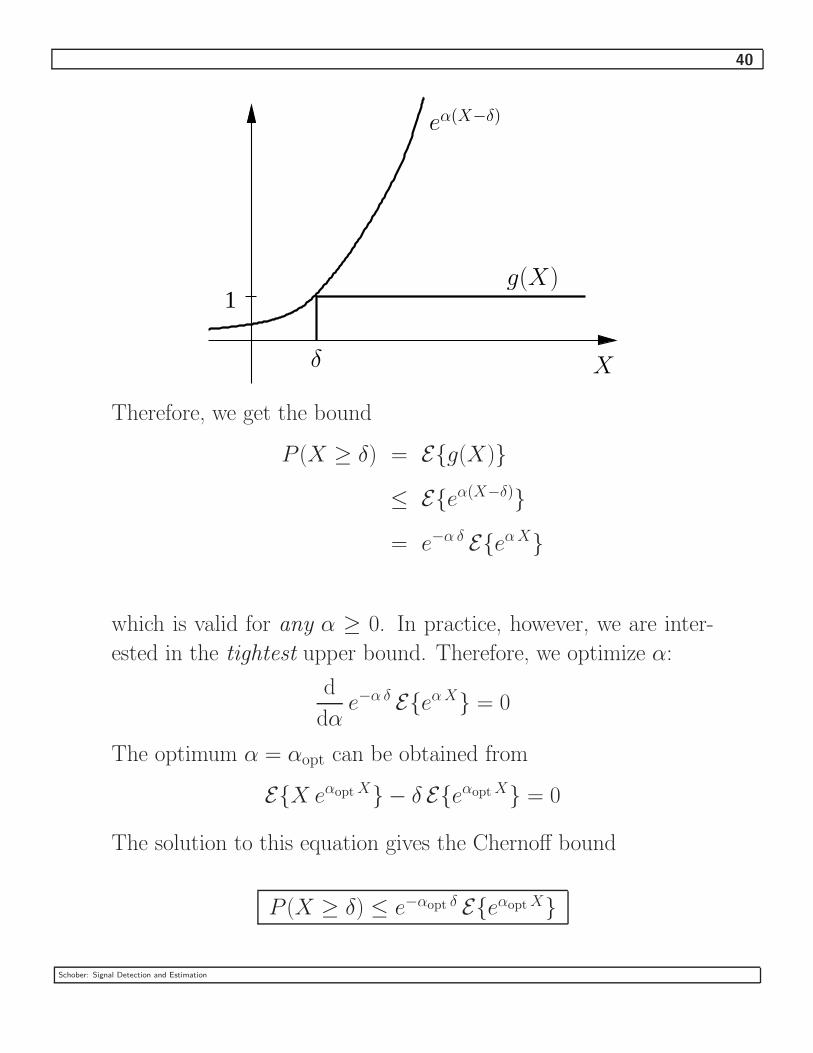
40

1

eα(X−δ)

g(X)

Xδ

Therefore, we get the bound

P (X ≥ δ) = E{g(X)}

≤ E{eα(X−δ)}

= e−α δ E{eαX}

which is valid for any α ≥ 0. In practice, however, we are inter-

ested in the tightest upper bound. Therefore, we optimize α:

d

dαe−α δ E{eαX} = 0

The optimum α = αopt can be obtained from

E{X eαoptX} − δ E{eαoptX} = 0

The solution to this equation gives the Chernoff bound

P (X ≥ δ) ≤ e−αopt δ E{eαoptX}


41

2.1.7 Central Limit Theorem

� Given: n statistical independent and identically distributed RVs

Xi, i = 1, 2, . . . , n, with finite varuance. For simplicity, we as-

sume that the Xi have zero mean and identical variances σ2X . Note

that the Xi can have any PDF.

� We consider the sum

Y =1√n

n∑i=1

Xi

� Central Limit Theorem

For n→ ∞ Y is a Gaussian RV with zero mean and variance σ2X .

Proof: See Textbook

� In practice, already for small n (e.g. n = 5) the distribution of Y

is very close to a Gaussian PDF.

� In practice, it is not necessary that all Xi have exactly the same

PDF and the same variance. Also the statistical independence of

different Xi is not necessary. If the PDFs and the variances of

the Xi are similar, for sufficiently large n the PDF of Y can be

approximated by a Gaussian PDF.

� The central limit theorem explains why many physical phenomena

follow a Gaussian distribution.


42

2.2 Stochastic Processes

� In communications many phenomena (noise from electronic de-

vises, transmitted symbol sequence, etc.) can be described as RVs

X(t) that depend on (continuous) time t. X(t) is referred to as a

stochastic process.

� A single realization of X(t) is a sample function. E.g. measure-

ment of noise voltage generated by a particular resistor.

� The collection of all sample functions is the ensemble of sample

functions. Usually, the size of the ensemble is infinite.

� If we consider the specific time instants t1 > t2 > . . . > tn with

the arbitrary positive integer index n, the random variables Xti =

X(ti), i = 1, 2, . . . , n, are fully characterized by their joint PDF

p(xt1, xt2, . . . , xtn).

� Stationary stochastic process:

Consider a second set Xti+τ = X(ti+ τ ), i = 1, 2, . . . , n, of RVs,

where τ is an arbitrary time shift. If Xti and Xti+τ have the same

statistical properties, X(t) is stationary in the strict sense. In

this case,

p(xt1, xt2, . . . , xtn) = p(xt1+τ , xt2+τ , . . . , xtn+τ)

is true, where p(xt1+τ , xt2+τ , . . . , xtn+τ ) denotes the joint PDF of

the RVs Xti+τ . If Xti and Xti+τ do not have the same statistical

properties, the process X(t) is nonstationary.


43

2.2.1 Statistical Averages

� Statistical averages (= ensemble averages) of stochastic processes

are defined as averages with respect to the RVs Xti = X(ti).

� First order moment (mean):

m(ti) = E{Xti} =

∞∫

−∞

xti p(xti) dxti

For a stationary processes m(ti) = m is valid, i.e., the mean does

not depend on time.

� Second order moment: Autocorrelation function (ACF) φ(t1, t2)

φ(t1, t2) = E{Xt1Xt2} =

∞∫

−∞

∞∫

−∞

xt1 xt2 p(xt1, xt2) dxt1dxt2

For a stationary process φ(t1, t2) does not depend on the specific

time instances t1, t2, but on the difference τ = t1 − t2:

E{Xt1Xt2} = φ(t1, t2) = φ(t1 − t2) = φ(τ )

Note that φ(τ ) = φ(−τ ) (φ(·) is an even function) since E{Xt1Xt2} =

E{Xt2Xt1} is valid.


44

Example:

ACF of an uncorrelated stationary process: φ(τ ) = δ(τ )

1

τ

φ(τ )

� Central second order moment: Covariance function µ(t1, t2)

µ(t1, t2) = E{(Xt1 −m(t1))(Xt2 −m(t2))}

= φ(t1, t2) −m(t1)m(t2)

For a stationary processes we get

µ(t1, t2) = µ(t1 − t2) = µ(τ ) = φ(τ ) −m2

� Stationary stochastic processes are asymptotically uncorrelated,

i.e.,

limτ→∞

µ(τ ) = 0


45

� Average power of stationary process:

E{X2t } = φ(0)

� Variance of stationary processes:

E{(Xt −m)2} = µ(0)

� Wide–sense stationarity:

If the first and second order moments of a stochastic process are

invariant to any time shift τ , the process is referred to as wide–

sense stationary process. Wide–sense stationary processes are not

necessarily stationary in the strict sense.

� Gaussian process:

Since Gaussian RVs are fully specified by their first and second

order moments, in this special case wide–sense stationarity auto-

matically implies stationarity in the strict sense.

� Ergodicity:

We refer to a process X(t) as ergodic if its statistical averages

can also be calculated as time–averages of sample functions. Only

(wide–sense) stationary processes can be ergodic.

For example, if X(t) is ergodic and one of its sample functions

(i.e., one of its realizations) is denoted as x(t), the mean and the


46

ACF can be calulated as

m = limT→∞

1

2T

T∫

−T

x(t) dt

and

φ(τ ) = limT→∞

1

2T

T∫

−T

x(t)x(t+ τ ) dt,

respectively. In practice, it is usually assumed that a process is

(wide–sense) stationary and ergodic. Ergodicity is important since

in practice only sample functions of a stochastic process can be

observed!

Averages for Jointly Stochastic Processes

� Let X(t) and Y (t) denote two stochastic processes and consider

the RVs Xti = X(ti), i = 1, 2, . . . , n, and Yt′j

= Y (t′j), j =

1, 2, . . . , m at times t1 > t2 > . . . > tn and t′1 > t′2 > . . . > t′m,

respectively. The two stochastic processes are fully characterized

by their joint PDF

p(xt1, xt2, . . . , xtn, yt′1, yt′2, . . . , yt′m)

� Joint stationarity: X(t) and Y (t) are jointly stationary if their

joint PDF is invariant to time shifts τ for all n and m.


47

� Cross–correlation function (CCF): φXY (t1, t2)

φXY (t1, t2) = E{Xt1Yt2} =

∞∫

−∞

∞∫

−∞

xt1 yt2 p(xt1, yt2) dxt1dyt2

If X(t) and Y (t) are jointly and individually stationary, we get

φXY (t1, t2) = E{Xt1Yt2} = E{Xt2+τYt2} = φXY (τ )

with τ = t1 − t2. We can establish the symmetry relation

φXY (−τ ) = E{Xt2−τYt2} = E{Yt′2+τXt′2

} = φY X(τ )

� Cross–covariance function µXY (t1, t2)

µXY (t1, t2) = E{(Xt1 −mX(t1))(Yt2 −mY (t2))}

= φXY (t1, t2) −mX(t1)mY (t2)

If X(t) and Y (t) are jointly and individually stationary, we get

µXY (t1, t2) = E{(Xt1 −mX)(Yt2 −mY )} = µXY (τ )

with τ = t1 − t2.


48

� Statistical independence

Two processes X(t) and Y (t) are statistical independent if and

only if

p(xt1, xt2, . . . , xtn, yt′1, yt′2, . . . , yt′m) =

p(xt1, xt2, . . . , xtn) p(yt′1, yt′2, . . . , yt′m)

is valid for all n and m.

� Uncorrelated processes

Two processes X(t) and Y (t) are uncorrelated if and only if

µXY (t1, t2) = 0

holds.

Complex Stochastic Processes

� Given: Complex random process Z(t) = X(t) + jY (t) with real

random processes X(t) and Y (t)

� Similarly to RVs, we treat Z(t) as a tupel of X(t) and Y (t), i.e.,

the PDF of Zti = Z(ti), 1, 2, . . . , n is given by

pZ(zt1, zt2, . . . , ztn) = pXY (xt1, xt2, . . . , xtn, yt1, yt2, . . . , ytn)

� We define the ACF of a complex–valued stochastic process Z(t)


49

as

φZZ(t1, t2) = E{Zt1Z∗t2}

= E{(Xt1 + jYt1)(Xt2 − jYt2)}

= φXX(t1, t2) + φY Y (t1, t2) + j(φY X(t1, t2) − φXY (t1, t2))

where φXX(t1, t2), φY Y (t1, t2) and φY X(t1, t2), φXY (t1, t2) denote

the ACFs and the CCFs of X(t) and Y (t), respectively.

Note that our definition of φZZ(t1, t2) differs from the Textbook,

where φZZ(t1, t2) = 12E{Zt1Z

∗t2} is used!

If Z(t) is a stationary process we get

φZZ(t1, t2) = φZZ(t2 + τ, t2) = φZZ(τ )


We can also establish the symmetry relation

φZZ(τ ) = φ∗ZZ(−τ )

� CCF of processes Z(t) and W (t)

φZW (t1, t2) = E{Zt1W∗t2}

If Z(t) and W (t) are jointly and individually stationary we have

φZW (t1, t2) = φZW (t2 + τ, t2) = φZW (τ )

Symmetry:

φ∗ZW (τ ) = E{Z∗t2+τ

Wt2} = E{Wt′2−τZ∗

t′2} = φWZ(−τ )


50

2.2.2 Power Density Spectrum

� The Fourier spectrum of a random process does not exist.

� Instead we define the power spectrum of a stationary stochastic

process as the Fourier transform F{·} of the ACF

Φ(f) = F{φ(τ )} =

∞∫

−∞

φ(τ ) e−j2πfτ dτ

Consequently, the ACF can be obtained from the power spectrum

(also referred to as power spectral density) via inverse Fourier

transform F−1{·} as

φ(τ ) = F−1{Φ(f)} =

∞∫

−∞

Φ(f) ej2πfτ df

Example:

Power spectrum of an uncorrelated stationary process:

Φ(f) = F{δ(τ )} = 1

1

f

Φ(f)


51

� The average power of a stationary stochastic process can be ob-

tained as

φ(0) =

∞∫

−∞

Φ(f) df

= E{|Xt|2} ≥ 0

Symmetry of power density spectrum:

Φ∗(f) =

∞∫

−∞

φ∗(τ ) ej2πfτ dτ

=

∞∫

−∞

φ∗(−τ ) e−j2πfτ dτ

=

∞∫

−∞

φ(τ ) e−j2πfτ dτ

= Φ(f)

This means Φ(f) is a real–valued function.


52

� Cross–correlation spectrum

Consider the random processes X(t) and Y (t) with CCF φXY (τ ).

The cross–correlation spectrum ΦXY (f) is defined as

ΦXY (f) =

∞∫

−∞

φXY (τ ) e−j2πfτ dτ

It can be shown that the symmetry relation Φ∗XY (f) = ΦY X(f)

is valid. If X(t) and Y (t) are real stochastic processes ΦY X(f) =

ΦXY (−f) holds.

2.2.3 Response of a Linear Time–Invariant System to a Ran-

dom Input Signal

� We consider a deterministic linear time–invariant system fully de-

scribed by its impulse response h(t), or equivalently by its fre-

quency response

H(f) = F{h(t)} =

∞∫

−∞

h(t) e−j2πft dt

� Let the signal x(t) be the input to the system h(t). Then the

output y(t) of the system can be expressed as

y(t) =

∞∫

−∞

h(τ ) x(t− τ ) dτ


53

In our case x(t) is a sample function of a (stationary) stochastic

processX(t) and therefore, y(t) is a sample function of a stochastic

process Y (t). We are interested in the mean and the ACF of Y (t).

� Mean of Y (t)

mY = E{Y (t)} =

∞∫

−∞

h(τ ) E{X(t− τ )} dτ

= mX

∞∫

−∞

h(τ ) dτ = mX H(0)

� ACF of Y (t)

φY Y (t1, t2) = E{Yt1Y∗t2}

=

∞∫

−∞

∞∫

−∞

h(α)h∗(β) E{X(t1 − α)X∗(t2 − β)} dα dβ

=

∞∫

−∞

∞∫

−∞

h(α)h∗(β)φXX(t1 − t2 + β − α) dα dβ

=

∞∫

−∞

∞∫

−∞

h(α)h∗(β)φXX(τ + β − α) dα dβ

= φY Y (τ )


54

Here, we have used τ = t1 − t2 and the last line indicates that if

the input to a linear time–invariant system is stationary, also the

output will be stationary.

If we define the deterministic system ACF as

φhh(τ ) = h(τ ) ∗ h∗(−τ ) =

∞∫

−∞

h∗(t)h(t + τ ) dt,

where ”∗” is the convolution operator, then we can rewrite φY Y (τ )

elegantly as

φY Y (τ ) = φhh(τ ) ∗ φXX(τ )

� Power spectral density of Y (t)

Since the Fourier transform of φhh(τ ) = h(τ ) ∗ h∗(−τ ) is

Φhh(f) = F{φhh(τ )} = F{h(τ ) ∗ h∗(−τ )}

= F{h(τ )}F{h∗(−τ )}

= |H(f)|2,

it is easy to see that the power spectral density of Y (t) is

ΦY Y (f) = |H(f)|2 ΦXX(f)

Since φY Y (0) = E{|Yt|2} = F−1{ΦY Y (f)}|τ=0,

φY Y (0) =

∞∫

−∞

ΦXX(f)|H(f)|2 df ≥ 0


55

is valid.

As an example, we may choose H(f) = 1 for f1 ≤ f ≤ f2 and

H(f) = 0 outside this interval, and obtain

f2∫

f1

ΦXX(f) df ≥ 0

Since this is only possible if ΦXX(f) ≥ 0, ∀ f , we conclude that

power spectral densities are non–negative functions of f .

� CCF between Y (t) and X(t)

φY X(t1, t2) = E{Yt1X∗t2} =

∞∫

−∞

h(α) E{X(t1 − α)X∗(t2)} dα

=

∞∫

−∞

h(α)φXX(t1 − t2 − α) dα

= h(τ ) ∗ φXX(τ )

= φY X(τ )


� Cross–spectrum

ΦY X(f) = F{φY X(τ )} = H(f) ΦXX(f)


56

2.2.4 Sampling Theorem for Band–Limited Stochastic Pro-

cesses

� A deterministic signal s(t) is called band–limited if its Fourier

transform S(f) = F{s(t)} vanishes identically for |f | > W . If

we sample s(t) at a rate higher than fs ≥ 2W , we can reconstruct

s(t) from the samples s(n/(2W )), n = 0, ±1, ±2, . . ., using an

ideal low–pass filter with bandwidth W .

� A stationary stochastic process X(t) is band–limited if its power

spectrum Φ(f) vanishes identically for |f | > W , i.e., Φ(f) = 0 for

|f | > W . Since Φ(f) is the Fourier transform of φ(τ ), φ(τ ) can be

reconstructed from the samples φ(n/(2W )), n = 0, ±1, ±2, . . .:

φ(τ ) =

∞∑n=−∞

φ( n

2W

)sin [2πW (τ − n/(2W ))]

2πW (τ − n/(2W ))

h(t) = sin(2πWt)/(2πWt) is the impulse response of an ideal

low–pass filter with bandwidth W .

If X(t) is a band–limited stationary stochastic process, then we

can represent X(t) as

X(t) =∞∑

n=−∞

X( n

2W

)sin [2πW (t− n/(2W ))]

2πW (t− n/(2W )),

whereX(n/(2W )) are the samples ofX(t) at times n = 0, ±1, ±2, . . .


57

2.2.5 Discrete–Time Stochastic Signals and Systems

� Now, we consider discrete–time (complex) stochastic processesX [n]

with discrete–time n which is an integer. Sample functions of X [n]

are denoted by x[n]. X [n] may be obtained from a continuous–

time process X(t) by sampling X [n] = X(nT ), T > 0.

� X [n] can be characterized in a similar way as the continuous–time

process X(t).

� ACF

φ[n, k] = E{XnX∗k} =

∞∫

−∞

∞∫

−∞

xnx∗k p(xn, xk) dxndxk

If X [n] is stationary, we get

φ[λ] = φ[n, k] = φ[n, n− λ]

The average power of the stationary process X [n] is defined as

E{|Xn|2} = φ[0]

� Covariance function

µ[n, k] = φ[n, k] − E{Xn}E{X∗k}

If X [n] is stationary, we get

µ[λ] = φ[λ] − |mX |2,

where mX = E{Xn} denotes the mean of X [n].


58

� Power spectrum

The power spectrum of X [n] is the (discrete–time) Fourier trans-

form of the ACF φ[λ]

Φ(f) = F{φ[λ]} =∞∑

λ=−∞

φ[λ]e−j2πfλ

and the inverse transform is

φ[λ] = F−1{Φ(f)} =

1/2∫

−1/2

Φ(f) ej2πfλ df

Note that Φ(f) is periodic with a period fd = 1, i.e., Φ(f + k) =

Φ(f) for k = ±1, ±2, . . .

Example:

Consider a stochastic process with ACF

φ[λ] = p δ[λ + 1] + δ[λ] + p δ[λ− 1]

with constant p. The corresponding power spectrum is given

by

Φ(f) = F{φ[λ]} = 1 + 2cos(2πf).

Note that φ[λ] is a valid ACF if and only if −1/2 ≤ p ≤ 1/2.


59

� Response of a discrete–time linear time–invariant system

– Discrete–time linear time–invariant system is described by its

impulse response h[n]

– Frequency response

H(f) = F{h[n]} =∞∑

n=−∞

h[n] e−j2πfn

– Response y[n] of system to sample function x[n]

y[n] = h[n] ∗ x[n] =

∞∑k=−∞

h[k]x[n− k]

where ∗ denotes now discrete–time convolution.

– Mean of Y [n]

mY = E{Y [n]} =

∞∑k=−∞

h[k] E{X [n− k]}

= mX

∞∑k=−∞

h[k]

= mX H(0)

where mX is the mean of X [n].


60

– ACF of Y [n]

Using the deterministic ”system” ACF

φhh[λ] = h[λ] ∗ h∗[−λ] =

∞∑k=−∞

h∗[k]h[k + λ]

it can be shown that φY Y [λ] can be expressed as

φY Y [λ] = φhh[λ] ∗ φXX [λ]

– Power spectrum of Y [n]

ΦY Y (f) = |H(f)|2 ΦXX(f)

2.2.6 Cyclostationary Stochastic Processes

� An important class of nonstationary processes are cyclostationary

processes. Cyclostationary means that the statistical averages of

the process are periodic.

� Many digital communication signals can be expressed as

X(t) =∞∑

n=−∞

a[n] g(t− nT )

where a[n] denotes the transmitted symbol sequence and can be

modeled as a (discrete–time) stochastic process with ACF φaa[λ] =

E{a∗[n]a[n+λ]}. g(t) is a deterministic function. T is the symbol

duration.


61

� Mean of X(t)

mX(t) = E{X(t)}

=

∞∑n=−∞

E{a[n]} g(t− nT )

= ma

∞∑n=−∞

g(t− nT )

where ma is the mean of a[n]. Observe that mX(t+kT ) = mX(t),

i.e., mX(t) has period T .

� ACF of X(t)

φXX(t + τ, t) = E{X(t+ τ )X∗(t)}

=∞∑

n=−∞

∞∑m=−∞

E{a∗[n]a[m]} g∗(t− nT )g(t + τ −mT )

=∞∑

n=−∞

∞∑m=−∞

φaa[m− n] g∗(t− nT )g(t + τ −mT )

Observe again that

φXX(t + τ + kT, t + kT ) = φXX(t + τ, t)

and therefore the ACF has also period T .


62

� Time–average ACF

The ACF φXX(t+τ, t) depends on two parameters t and τ . Often

we are only interested in the time–average ACF defined as

φXX(τ ) =1

T

T/2∫

−T/2

φXX(t + τ, t) dt

� Average power spectrum

ΦXX(f) = F{φXX(τ )} =

∞∫

−∞

φXX(τ ) e−j2πfτ dτ


63

3 Characterization of Communication Signals and

Systems

3.1 Representation of Bandpass Signals and Systems

� Narrowband communication signals are often transmitted using

some type of carrier modulation.

� The resulting transmit signal s(t) has passband character, i.e., the

bandwidth B of its spectrum S(f) = F{s(t)} is much smaller

than the carrier frequency fc.

−fc fc

BS(f)

f

� We are interested in a representation for s(t) that is independent

of the carrier frequency fc. This will lead us to the so–called equiv-

alent (complex) baseband representation of signals and systems.


64

3.1.1 Equivalent Complex Baseband Representation of Band-

pass Signals

� Given: Real–valued bandpass signal s(t) with spectrum

S(f) = F{s(t)}

� Analytic Signal s+(t)

In our quest to find the equivalent baseband representation of s(t),

we first suppress all negative frequencies in S(f), since S(f) =

S(−f) is valid.

The spectrum S+(f) of the resulting so–called analytic signal

s+(t) is defined as

S+(f) = F{s+(t)} = 2 u(f)S(f),

where u(f) is the unit step function

u(f) =

0, f < 0

1/2, f = 0

1, f > 0

.

1

1/2

f

u(f)


65

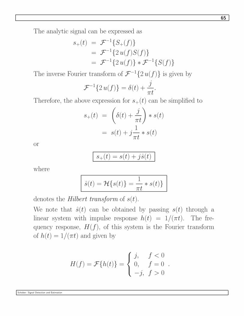
The analytic signal can be expressed as

s+(t) = F−1{S+(f)}

= F−1{2 u(f)S(f)}

= F−1{2 u(f)} ∗ F−1

{S(f)}

The inverse Fourier transform of F−1{2 u(f)} is given by

F−1{2 u(f)} = δ(t) +

j

πt.

Therefore, the above expression for s+(t) can be simplified to

s+(t) =

(δ(t) +

j

πt

)∗ s(t)

= s(t) + j1

πt∗ s(t)

or

s+(t) = s(t) + js(t)

where

s(t) = H{s(t)} =1

πt∗ s(t)}

denotes the Hilbert transform of s(t).

We note that s(t) can be obtained by passing s(t) through a

linear system with impulse response h(t) = 1/(πt). The fre-

quency response, H(f), of this system is the Fourier transform

of h(t) = 1/(πt) and given by

H(f) = F{h(t)} =

j, f < 0

0, f = 0

−j, f > 0

.


66

f

H(f)

−j

j

The spectrum S(f) = F{s(t)} can be obtained from

S(f) = H(f)S(f)

� Equivalent Baseband Signal sb(t)

We obtain the equivalent baseband signal sb(t) from s+(t) by

frequency translation (and scaling), i.e., the spectrum Sb(f) =

F{sb(t)} of sb(t) is defined as

Sb(f) =1√

2S+(f + fc),

where fc is an appropriately chosen translation frequency. In prac-

tice, if passband signal s(t) was obtained through carrier modu-

lation, it is often convenient to choose fc equal to the carrier fre-

quency.

Note: Our definition of the equivalent baseband signal is different

from the definition used in the textbook. In particular, the factor1√2

is missing in the textbook. Later on it will become clear why

it is convenient to introduce this factor.


67

Example:

1

2

√2

S+(f)

S(f)

Sb(f)

f

f

f

−fc fc

fc

The equivalent baseband signal sb(t) (also referred to as complex

envelope of s(t)) itself is given by

sb(t) = F−1{Sb(f)} =

1√

2s+(t) e−j2πfct,

which leads to

sb(t) =1√

2[s(t) + js(t)] e−j2πfct


68

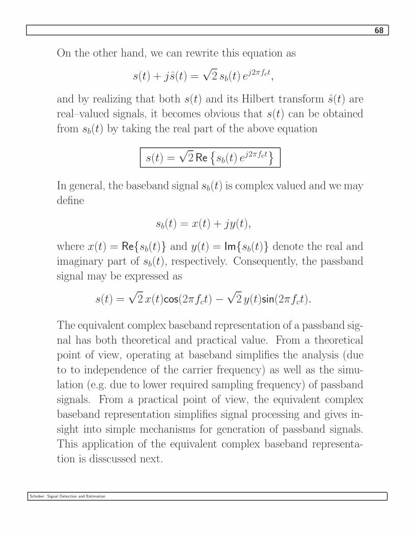
On the other hand, we can rewrite this equation as

s(t) + js(t) =√

2 sb(t) ej2πfct,

and by realizing that both s(t) and its Hilbert transform s(t) are

real–valued signals, it becomes obvious that s(t) can be obtained

from sb(t) by taking the real part of the above equation

s(t) =√

2 Re{sb(t) ej2πfct

}

In general, the baseband signal sb(t) is complex valued and we may

define

sb(t) = x(t) + jy(t),

where x(t) = Re{sb(t)} and y(t) = Im{sb(t)} denote the real and

imaginary part of sb(t), respectively. Consequently, the passband

signal may be expressed as

s(t) =√

2 x(t)cos(2πfct) −√

2 y(t)sin(2πfct).

The equivalent complex baseband representation of a passband sig-

nal has both theoretical and practical value. From a theoretical

point of view, operating at baseband simplifies the analysis (due

to to independence of the carrier frequency) as well as the simu-

lation (e.g. due to lower required sampling frequency) of passband

signals. From a practical point of view, the equivalent complex

baseband representation simplifies signal processing and gives in-

sight into simple mechanisms for generation of passband signals.

This application of the equivalent complex baseband representa-

tion is disscussed next.


69

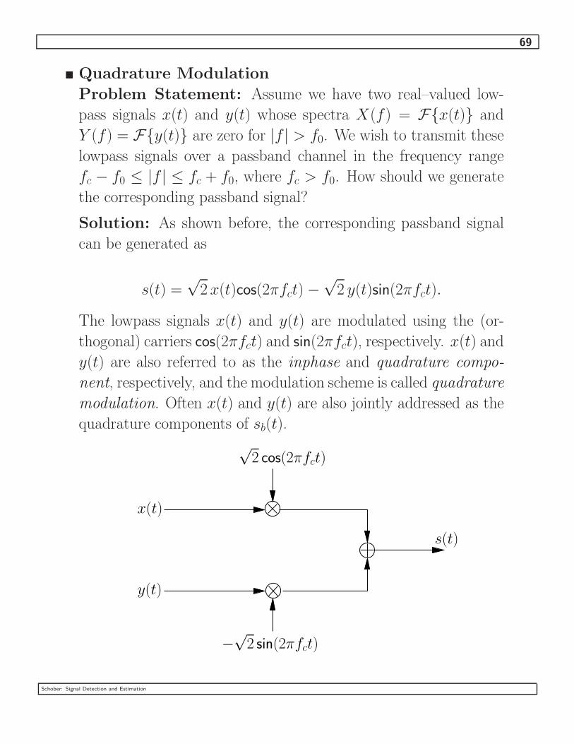
� Quadrature Modulation

Problem Statement: Assume we have two real–valued low-

pass signals x(t) and y(t) whose spectra X(f) = F{x(t)} and

Y (f) = F{y(t)} are zero for |f | > f0. We wish to transmit these

lowpass signals over a passband channel in the frequency range

fc − f0 ≤ |f | ≤ fc + f0, where fc > f0. How should we generate

the corresponding passband signal?

Solution: As shown before, the corresponding passband signal

can be generated as

s(t) =√

2 x(t)cos(2πfct) −√

2 y(t)sin(2πfct).

The lowpass signals x(t) and y(t) are modulated using the (or-

thogonal) carriers cos(2πfct) and sin(2πfct), respectively. x(t) and

y(t) are also referred to as the inphase and quadrature compo-

nent, respectively, and the modulation scheme is called quadrature

modulation. Often x(t) and y(t) are also jointly addressed as the

quadrature components of sb(t).

y(t)

√2 cos(2πfct)

−√

2 sin(2πfct)

s(t)

x(t)


70

� Demodulation

At the receiver side, the quadrature components x(t) and y(t) have

to be extracted from the passband signal s(t).

Using the relation

sb(t) = x(t) + jy(t) =1√

2[s(t) + js(t)] e−j2πfct,

we easily get

x(t) =1√

2[s(t)cos(2πfct) + s(t)sin(2πfct)]

y(t) =1√

2[s(t)cos(2πfct) − s(t)sin(2πfct)]

Hilbert

+

+

+

−Transform

x(t)

y(t)

s(t) 1√2sin(2πfct)

1√2cos(2πfct)

Unfortunately, the above structure requires a Hilbert transformer

which is difficult to implement.

Fortunately, if Sb(f) = 0 for |f | > f0 and fc > f0 are valid, i.e., if

x(t) and y(t) are bandlimited, x(t) and y(t) can be obtained from

s(t) using the structure shown below.


71

−√

2 sin(2πfct)

s(t)

x(t)

y(t)

HLP(f)

HLP(f)

√2 cos(2πfct)

HLP(f) is a lowpass filter. With cut–off frequency fLP, f0 ≤

fLP ≤ 2fc − f0. The above structure is usually used in practice to

transform a passband signal into (complex) baseband.

1

f

HLP(f)

−fLP fLP


72

� Energy of sb(t)

For calculation of the energy of sb(t), we need to express the spec-

trum S(f) of s(t) as a function of Sb(f):

S(f) = F{s(t)}

=

∞∫

−∞

Re

{√2sb(t)e

j2πfct}

e−j2πft dt

=

√2

2

∞∫

−∞

(sb(t)e

j2πfct + s∗b(t)e−j2πfct

)e−j2πft dt

=1√

2[Sb(f − fc) + S∗

b (−f − fc)]

Now, using Parsevals Theorem we can express the energy of s(t)

as

E =

∞∫

−∞

s2(t) dt =

∞∫

−∞

|S(f)|2 df

=

∞∫

−∞

∣∣∣∣ 1√

2[Sb(f − fc) + S∗

b (−f − fc)]

∣∣∣∣2

df

=1

2

∞∫

−∞

[|Sb(f − fc)|

2 + |S∗b (−f − fc)|

2 +

Sb(f − fc)Sb(−f − fc) + S∗b (f − fc)S

∗b (−f − fc)

]df


73

It is easy to show that

∞∫

−∞

|Sb(f − fc)|2 df =

∞∫

−∞

|S∗b (−f − fc)|

2 df =

∞∫

−∞

|Sb(f)|2 df

is valid. In addition, if the spectra Sb(f − fc) and Sb(−f − fc)

do not overlap, which will be usually the case in practice since the

bandwidth B of Sb(f) is normally much smaller than fc, Sb(f −

fc)Sb(−f − fc) = 0 is valid.

Using these observations the energy E of s(t) can be expressed as

E =

∞∫

−∞

|Sb(f)|2 df =

∞∫

−∞

|sb(t)|2 dt

To summarize, we have show that energy of the baseband signal is

identical to the energy of the corresponding passband signal

E =

∞∫

−∞

s2(t) dt =

∞∫

−∞

|sb(t)|2 dt

Note: This identity does not hold for the baseband transforma-

tion used in the text book. Since the factor 1/√

2 is missing in the

definition of the equivalent baseband signal in the text book, there

the energy of sb(t) is twice that of the passband signal s(t).


74

3.1.2 Equivalent Complex Baseband Representation of Band-

pass Systems

� The equivalent baseband representation of systems is similar to

that of signals. However, there are a few minor but important

differences.

� Given: Bandpass system with impulse response h(t) and transfer

function H(f) = F{h(t)}.

� Analytic System

The transfer function H+(f) and impulse response h+(t) of the

analytic system are respectively defined as

H+(f) = 2u(f)H(f)

and

h+(t) = F−1{H+(f)},

which is identical to the corresponding definitions for analytic sig-

nals.

� Equivalent Baseband System

The transfer function Hb(f) of the equivalent baseband system is

defined as

Hb(f) =1

2H+(f + fc).

Note: This definition differs from the definition of the equivalent

baseband signal. Here, we have the factor 1/2, whereas we had

1/√

2 in the definition of the the equivalent baseband signal.


75

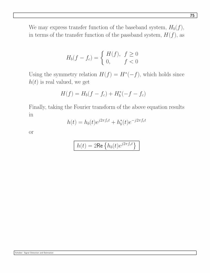
We may express transfer function of the baseband system, Hb(f),

in terms of the transfer function of the passband system, H(f), as

Hb(f − fc) =

{H(f), f ≥ 0

0, f < 0

Using the symmetry relation H(f) = H∗(−f), which holds since

h(t) is real valued, we get

H(f) = Hb(f − fc) + H∗b (−f − fc)

Finally, taking the Fourier transform of the above equation results

in

h(t) = hb(t)ej2πfct + h∗

b(t)e−j2πfct

or

h(t) = 2Re{hb(t)e

j2πfct}


76

3.1.3 Response of a Bandpass Systems to a Bandpass Signal

Objective: In this section, we try to find out whether linear filtering

in complex baseband is equivalent to the same operation in passband.

equivalent?

s(t) h(t) r(t)

rb(t)hb(t)sb(t)

Obviously, we have

R(f) = F{r(t)} = H(f)S(f)

=1√

2[Sb(f − fc) + S∗(−f − fc)] [Hb(f − fc) + H∗

b (−f − fc)]

Since both s(t) and h(t) have narrowband character

Sb(f − fc)H∗b (−f − fc) = 0

S∗b (−f − fc)Hb(f − fc) = 0

is valid, and we get

R(f) =1√

2[Sb(f − fc)Hb(f − fc) + S∗(−f − fc)H

∗b (−f − fc)]

=1√

2[Rb(f − fc) + R∗

b(−f − fc)]


77

This result shows that we can get the output r(t) of the linear system

h(t) by transforming the output rb(t) of the equivalent baseband system

hb(t) into passband. This is an important result since it shows that,

without loss of generality, we can perform linear filtering operations

always in the equivalent baseband domain. This is very convenient for

example if we want to simulate a communication system that operates

in passband using a computer.

3.1.4 Equivalent Baseband Representation of Bandpass Sta-

tionary Stochastic Processes

Given: Wide–sense stationary noise process n(t) with zero–mean and

power spectral density ΦNN(f). In particular, we assume a narrow-

band bandpass noise process with bandwidth B and center (carrier)

frequency fc, i.e.,

ΦNN(f)

{6= 0, fc − B/2 ≤ |f | ≤ fc + B/2

= 0, otherwise

B

fc−fc

ΦNN(f)

f


78

Equivalent Baseband Noise

Defining the equivalent complex baseband noise process

z(t) = x(t) + jy(t),

where x(t) and y(t) are real–valued baseband noise processes, we can

express the passband noise n(t) as

n(t) =√

2Re{z(t)ej2πfct

}=

√2 [x(t)cos(2πfct) − y(t)sin(2πfct)] .

Stationarity of n(t)

Since n(t) is assumed to be wide–sense stationary, the correlation func-

tions φXX(τ ) = E{x(t + τ )x∗(t)}, φY Y (τ ) = E{y(t + τ )y∗(t)}, and

φXY (τ ) = E{x(t + τ )y∗(t)} have to fulfill certain conditions as will be

shown in the following.

The ACF of n(t) is given by

φNN (τ, t + τ ) = E{n(t)n(t + τ )}

= E {2 [x(t)cos(2πfct) − y(t)sin(2πfct)]

[x(t + τ )cos(2πfc(t + τ )) − y(t + τ )sin(2πfc(t + τ ))]}

= [φXX(τ ) + φY Y (τ )] cos(2πfcτ )

+ [φXX(τ ) − φY Y (τ )] cos(2πfc(2t + τ ))

− [φY X(τ ) − φXY (τ )] sin(2πfcτ )

− [φY X(τ ) + φXY (τ )] sin(2πfc(2t + τ )),


79

where we have used the trigonometric relations

cos(α)cos(β) =1

2[cos(α − β) + cos(α + β)]

sin(α)sin(β) =1

2[cos(α − β) − cos(α + β)]

sin(α)sin(β) =1

2[sin(α − β) − sin(α + β)]

For n(t) to be a wide–sense stationary passband process, the equivalent

baseband process has to fulfill the conditions

φXX(τ ) = φY Y (τ )

φY X(τ ) = −φXY (τ )

Hence, the ACF of n(t) can be expressed as

φNN(τ ) = 2 [φXX(τ )cos(2πfcτ ) − φY X(τ )sin(2πfcτ )]

ACF of z(t)

Using the above conditions, the ACF φZZ(τ ) of z(t) is easily calculated

as

φZZ(τ ) = E{z(t + τ )z∗(t)}

= φXX(τ ) + φY Y (τ ) + j(φY X(τ ) − φXY (τ ))

= 2φXX(τ ) + j2φY X(τ )

As a consequence, we can express φNN (τ ) as

φNN(τ ) = Re{φZZ(τ )ej2πfcτ}


80

Power Spectral Density of n(t)

The power spectral densities of z(t) and n(t) are given by

ΦNN(f) = F{φNN(τ )}

ΦZZ(f) = F{φZZ(τ )}

Therefore, we can represent ΦNN(f) as

ΦNN(f) =

∞∫

−∞

Re{φZZ(τ )ej2πfcτ} e−j2πfτ dτ

=1

2[ΦZZ(f − fc) + ΦZZ(−f − fc)] ,

where we have used the fact that ΦZZ(f) is a real–valued function.

Properties of the Quadrature Components

From the stationarity of n(t) we derived the identity

φY X(τ ) = −φXY (τ )

On the other hand, the relation

φY X(τ ) = φXY (−τ )

holds for any wide–sense stationary stochastic process. If we combine

these two relations, we get

φXY (τ ) = −φXY (−τ ),

i.e., φXY (τ ) is an odd function in τ , and φXY (0) = 0 holds always.

If the quadrature components x(t) and y(t) are uncorrelated, their

correlation function is zero, φXY (τ ) = 0, ∀τ . Consequently, the ACF

of z(t) is real valued

φZZ(τ ) = 2φXX(τ )


81

From this property we can conclude that for uncorrelated quadrature

components the power spectral density of z(t) is symmetric about f =

0

ΦZZ(f) = ΦZZ(−f)

White Noise

In the region of interest (i.e., where the transmit signal has non–zero

frequency components), ΦNN(f) can often be approximated as flat,

i.e.,

ΦNN(f) =

{N0/2, fc − B/2 ≤ |f | ≤ fc + B/2

0, otherwise

N0/2

B

f−fc fc

ΦNN(f)

The power spectral density of the corresponding baseband noise process

z(t) is given by

ΦZZ(f) =

{N0, |f | ≤ B/2

0, otherwise


82

B2

N0

ΦZZ(f)

f−B2

and the ACF of z(t) is given by

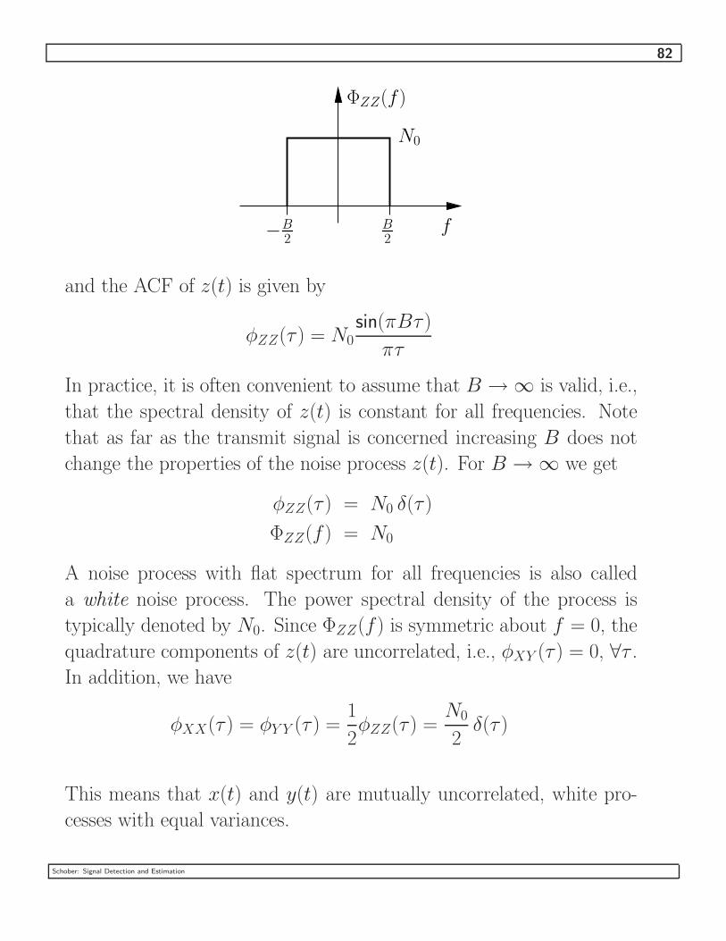
φZZ(τ ) = N0sin(πBτ )

πτ

In practice, it is often convenient to assume that B → ∞ is valid, i.e.,

that the spectral density of z(t) is constant for all frequencies. Note

that as far as the transmit signal is concerned increasing B does not

change the properties of the noise process z(t). For B → ∞ we get

φZZ(τ ) = N0 δ(τ )

ΦZZ(f) = N0

A noise process with flat spectrum for all frequencies is also called

a white noise process. The power spectral density of the process is

typically denoted by N0. Since ΦZZ(f) is symmetric about f = 0, the

quadrature components of z(t) are uncorrelated, i.e., φXY (τ ) = 0, ∀τ .

In addition, we have

φXX(τ ) = φY Y (τ ) =1

2φZZ(τ ) =

N0

2δ(τ )

This means that x(t) and y(t) are mutually uncorrelated, white pro-

cesses with equal variances.


83

Note that although white noise is convenient for analysis, it is not phys-

ically realizable since it would have an infinite variance.

White Gaussian Noise

For most applications it can be assumed that the channel noise n(t) is

not only stationary and white but also Gaussian distributed. Conse-

quently, the quadrature components x(t) and y(t) of z(t) are mutually

uncorrelated white Gaussian processes.

Observed through a lowpass filter with bandwidth B, x(t) and y(t)

have equal variances σ2 = φXX(0) = φY Y (0) = N0B/2. The PDF of

corresponding filtered complex process z(t0) = z = x + jy is given by

pZ(z) = pXY (x, y)

=1

2πσ2exp

(−

x2 + y2

2σ2

)

=1

πσ2Z

exp

(−|z|2

σ2Z

),

where σ2Z = 2σ2 is valid. Since this PDF is rotationally symmetric, the

corresponding equivalent baseband noise process is also referred to as

circularly symmetric complex Gaussian noise.

z(t) z(t)HLP(f)

From the above considerations we conclude that if we want to analyze

or simulate a passband communication system that is impaired by sta-

tionary white Gaussian noise, the corresponding equivalent baseband

noise has to be circularly symmetric white Gaussian noise.


84

Overall System Model

From the considerations in this section we can conclude that a pass-

band system, including linear filters and wide–sense stationary noise,

can be equivalently represented in complex baseband. The baseband

representation is useful for simulation and analysis of passband sys-

tems.

equivalent

z(t)

s(t) r(t)h(t)

sb(t) rb(t)hb(t)

n(t)


85

3.2 Signal Space Representation of Signals

� Signals can be represented as vectors over a certain basis.

� This description allows the application of many well–known tools

(inner product, notion of orthogonality, etc.) from Linear Algebra

to signals.

3.2.1 Vector Space Concepts – A Brief Review

� Given: n–dimensional vector

v = [v1 v2 . . . vn]T

=

n∑i=1

viei,

with unit or basis vector

ei = [0 . . . 0 1 0 . . . 0]T ,

where 1 is the ith element of ei.

� Inner Product v1 • v2

We define the (complex) vector vj, j ∈ {1, 2}, as

vj = [vj1 vj2 . . . vjn]T .

The inner product between v1 and v2 is defined as

v1 • v2 = vH2 v1

=

n∑i=1

v∗2iv1i


86

Two vectors are orthogonal if and only if their inner product is

zero, i.e.,

v1 • v2 = 0

� L2–Norm of a Vector

The L2–norm of a vector v is defined as

||v|| =√

v • v =

√√√√ n∑i=1

|vi|2

� Linear Independence

Vector x is linearly independent of vectors vj, 1 ≤ j ≤ n, if there

is no set of coefficients aj, 1 ≤ j ≤ n, for which

x =

n∑j=1

ajvj

is valid.

� Triangle Inequality

The triangle inequality states that

||v1 + v2|| ≤ ||v1|| + ||v2||,

where equality holds if and only if v1 = a v2, where a is positive

real valued, i.e., a ≥ 0.

� Cauchy–Schwarz Inequality

The Cauchy–Schwarz inequality states that

|v1 • v2| ≤ ||v1|| ||v2||

is true. Equality holds if v1 = b v2, where b is an arbitrary

(complex–valued) scalar.


87

� Gram–Schmidt Procedure

– Enables construction of an orthonormal basis for a given set

of vectors.

– Given: Set of n–dimensional vectors vj, 1 ≤ j ≤ m, which

span an n1–dimensional vector space with n1 ≤ max{n, m}.

– Objective: Find orthonormal basis vectors uj, 1 ≤ j ≤ n1.

– Procedure:

1. First Step: Normalize first vector of set (the order is arbi-

trary).

u1 =v1

||v1||

2. Second Step: Identify that part of v2 which is orthogonal

to u1.

u′2 = v2 − (v2 • u1) u1,

where (v2 • u1) u1 is the projection of v2 onto u1. There-

fore, it is easy to show that u′2 •u1 = 0 is valid. Thus, the

second basis vector u2 is obtained by normalization of u′2

u2 =u′

2

||u′2||

3. Third Step:

u′3 = v3 − (v3 • u1) u1 − (v3 • u2) u2

u3 =u′

3

||u′3||

4. Repeat until vm has been processed.


88

– Remarks:

1. The number n1 of basis vectors is smaller or equal max{n, m},

i.e., n1 ≤ max{n, m}.

2. If a certain vector vj is linearly dependent on the previously

found basis vectors ui, 1 ≤ i ≤ j − 1, u′j = 0 results and

we proceed with the next element vj+1 of the set of vectors.

3. The found set of basis vectors is not unique. Different sets

of basis vectors can be found e.g. by changing the processing

order of the vectors vj, 1 ≤ j ≤ m.

3.2.2 Signal Space Concepts

Analogous to the vector space concepts discussed in the last section,

we can use similar concepts in the so–called signal space.

� Inner Product

The inner product of two (complex–valued) signals x1(t) and x2(t)

is defined as

< x1(t), x2(t) > =

b∫

a

x1(t)x∗2(t) dt, b ≥ a,

where a and b are real valued scalars.

� Norm

The norm of a signal x(t) is defined as

||x(t)|| =√

< x(t), x(t) > =

√√√√√b∫

a

|x(t)|2 dt.


89

� Energy

The energy of a signal x(t) is defined as

E = ||x(t)||2 =

∞∫

−∞

|x(t)|2 dt.

� Linear Independence

m signals are linearly independent if and only if no signal of the

set can be represented as a linear combination of the other m − 1

signals.

� Triangle Inequality

Similar to the vector space case the triangle inequality states

||x1(t) + x2(t)|| ≤ ||x1(t)|| + ||x2(t)||,

where equality holds if and only if x1(t) = ax2(t), a ≥ 0.

� Cauchy–Schwarz Inequality

| < x1(t), x2(t) > | ≤ ||x1(t)|| ||x2(t)||,

where equality holds if and only if x1(t) = bx2(t), where b is

arbitrary complex.


90

3.2.3 Orthogonal Expansion of Signals

For the design and analysis of communication systems it is often nec-

essary to represent a signal as a sum of orthogonal signals.

� Given:

– (Complex–valued) signal s(t) with finite energy

Es =

∞∫

−∞

|s(t)|2 dt

– Set of K orthonormal functions {fn(t), n = 1, 2, . . . , K}

< fn(t), fm(t) > =

∞∫

−∞

fn(t)f∗m(t) dt =

{1, n = m

0 n 6= m

� Objective:

Find “best” approximation for s(t) in terms of fn(t), 1 ≤ n ≤ K.

The approximation s(t) is given by

s(t) =

K∑n=1

snfn(t),

with coefficients sn, 1 ≤ n ≤ K. The optimality criterion adopted

for the approximation of s(t) is the energy of the error,

e(t) = s(t) − s(t),

which is to be minimized.


91

The error energy is given by

Ee =

∞∫

−∞

|e(t)|2 dt

=

∞∫

−∞

|s(t) −

K∑n=1

snfn(t)|2 dt

� Optimize Coefficients sn

In order to find the optimum coefficients sn, 1 ≤ n ≤ K, which

minimize Ee, we have to differentiate Ee with respect to s∗n, 1 ≤

n ≤ K,

∂Ee

∂s∗n=

∞∫

−∞

[s(t) −

K∑k=1

skfk(t)

]f∗

n(t) dt = 0, n = 1, . . . , K,

where we have used the following rules for complex differentiation

(z is a complex variable):

∂z∗

∂z∗= 1,

∂z

∂z∗= 0,

∂|z|2

∂z∗= z

Since the fn(t) are orthonormal, we get

sn =

∞∫

−∞

s(t)f∗n(t) dt = < s(t), fn(t) >, n = 1, . . . , K.

This means that we can interpret s(t) simply as the projection of

s(t) onto the K–dimensional subspace spanned by the functions

{fn(t)}.


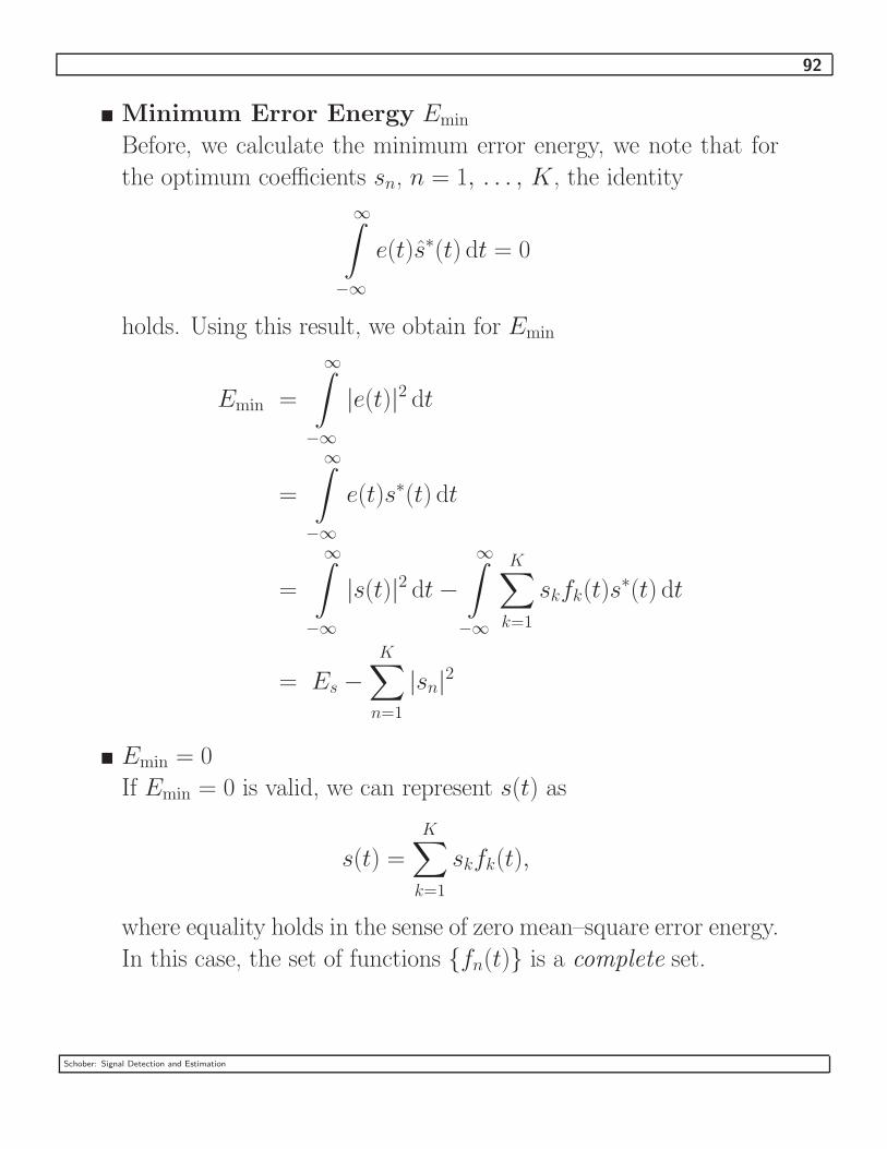
92

� Minimum Error Energy Emin

Before, we calculate the minimum error energy, we note that for

the optimum coefficients sn, n = 1, . . . , K, the identity

∞∫

−∞

e(t)s∗(t) dt = 0

holds. Using this result, we obtain for Emin

Emin =

∞∫

−∞

|e(t)|2 dt

=

∞∫

−∞

e(t)s∗(t) dt

=

∞∫

−∞

|s(t)|2 dt −

∞∫

−∞

K∑k=1

skfk(t)s∗(t) dt

= Es −

K∑n=1

|sn|2

� Emin = 0

If Emin = 0 is valid, we can represent s(t) as

s(t) =

K∑k=1

skfk(t),

where equality holds in the sense of zero mean–square error energy.

In this case, the set of functions {fn(t)} is a complete set.


93

� Gram–Schmidt Procedure

– Given: M signal waveforms {si(t), i = 1, . . . , M}.

– Objective: Construct a set of orthogonal waveforms {fi(t)}

from the original set {si(t)}.

– Procedure

1. First Step:

f1(t) =s1(t)√

E1

,

where the energy E1 of signal s1(t) is given by

E1 =

∞∫

−∞

|s1(t)|2 dt

2. Second Step:

Calculate the inner product of s2(t) and f1(t)

c12 =

∞∫

−∞

s2(t)f∗1 (t) dt

The projection of s2(t) onto f1(t) is simply c12f1(t). There-

fore, the function

f ′2(t) = s2(t) − c12f1(t)

is orthogonal to f1(t), i.e., < f1(t), f ′2(t) > = 0. A normal-

ized version of f ′2(t) gives the second basis function

f2(t) =f ′

2(t)√

E2

,


94

with

Ej =

∞∫

−∞

|f ′j(t)|

2 dt, j = 2, 3, . . .

3. kth Step

f ′k(t) = sk(t) −

k−1∑i=1

cikfi(t)

with

cik =

∞∫

−∞

sk(t)f∗i (t) dt

The kth basis function is obtained as

fk(t) =f ′

k(t)√Ek

,

4. The orthonormalization process continues until all M func-

tions of the set {si(t)} have been processed. The result are

N ≤ M orthonormal waveforms {fi(t)}.


95

Example:

Given are the following two signals

2

2 31 1

−1t

s2(t)s1(t)

t

1. First Step:

Signal s1(t) has energy

E1 =

∞∫

−∞

|s1(t)|2 dt = 2.

Therefore, the first basis function is

f1(t) =s1(t)√

E1

=s1(t)√

2

2

f1(t)

t

1√2

2. Second Step:

The inner product between the first basis function f1(t) and


96

the second signal s2(t) is

c12 =

∞∫

−∞

s2(t)f∗1 (t) dt =

1√

22.

Therefore, we obtain

f ′2(t) = s2(t) − c12f1(t)

= s2(t) − s1(t)

Since the energy of f ′2(t) is E2 = 1, the second basis function

is

f2(t) = s2(t) − s1(t)

2 3

f2(t)

−1t


97

� Representation of sk(t) by Basis Functions fk(t)

The original M signals sk(t) can be represented in terms of the N

orthogonal basis functions found by the Gram–Schmidt procedure.

In particular, we get

sk(t) =N∑

n=1

sknfn(t), k = 1, 2, . . . , M

with coefficients

skn =

∞∫

−∞

sk(t)f∗n(t) dt, n = 1, 2, . . . , N.

The energy Ek of the coefficient vector sk = [sk1 sk2 . . . skN ]T of

sk(t) is identical to the energy of sk(t) itself.

Ek =

∞∫

−∞

|sk(t)|2 dt =

N∑n=1

|skn|2 = ||sk||

2

� Signal Space Representation of sk(t)

For given basis vectors fn(t), 1 ≤ n ≤ N , the signals sk(t) are

fully described by their coefficient vector sk. The N orthonormal

basis functions span the N–dimensional signal space and vector sk

contains the coordinates of sk(t) in that signal space. Therefore, sk

is referred to as the signal space representation of sk(t). Using

the signal space representation of signals, many operations such

as correlation or energy calculation can be performed with vectors

instead of signals. This has the advantage that for example tedious

evaluations of integrals are avoided.


98

Example:

Continuation of previous example:

Since s1(t) =√

2f1(t), the signal space representation of s1(t) is

simply

s1 = [√

2 0]T .

For s21 and s22 we get, respectively,

s21 =

∞∫

−∞

s2(t)f∗1 (t) dt =

√2

and

s22 =

∞∫

−∞

s2(t)f∗2 (t) dt = 1.

Consequently, the signal space representation of s2(t) is

s2 = [√

2 1]T .

A graphical representation of the signal space for this example is

given below.

1

1

f2(t)

s2

s1f1(t)

Using the signal space representation, e.g. the inner product be-


99

tween s1(t) and s2(t) can be easily obtained as

< s1(t), s2(t) > = s1 • s2 =√

2√

2 + 0 · 1 = 2

� Complex Baseband Case

The passband signals sm(t), m = 1, 2, . . . , M , can be represented

by their complex baseband equivalents sbm(t) as

sm(t) =√

2Re{sbm(t)ej2πfct

}.

Recall that sm(t) and sbm(t) have the same energy

Em =

∞∫

−∞

s2m(t) dt =

∞∫

−∞

|sbm(t)|2 dt.

Inner Product

We express the inner product between sm(t) and sk(t) in terms of

the inner product between sbm(t) and sbk(t).∞∫

−∞

sm(t)s∗k(t) dt = 2

∞∫

−∞

Re{sbm(t)ej2πfct

}Re{sbk(t)e

j2πfct}

dt

=2

4

∞∫

−∞

(sbm(t)ej2πfct + s∗bm(t)e−j2πfct

)(sbk(t)e

j2πfct + s∗bk(t)e−j2πfct

)dt

Using a generalized form of Parsevals Theorem∞∫

−∞

x(t)y∗(t) dt =

∞∫

−∞

X(f)Y ∗(f) df


100

and the fact that both sm(t) and sk(t) are narrowband signals, the

above integral can be simplified to

∞∫

−∞

sm(t)s∗k(t) dt =1

2

∞∫

−∞

[Sbm(f − fc)S∗bk(f − fc) +

S∗bm(−f − fc)Sbk(−f − fc)] df

=1

2

∞∫

−∞

[Sbm(f)S∗bk(f) + S∗

bm(f)Sbk(f)] df

=1

2

∞∫

−∞

[sbm(t)s∗bk(t) + s∗bm(t)sbk(t)] dt

=

∞∫

−∞

Re {sbm(t)s∗bk(t)} dt

This result shows that the inner product of the passband signals is

identical to the real part of the inner product of the corresponding

baseband signals.

< sm(t), sk(t) > = Re{< sbm(t), sbk(t) >}

If we have a signal space representation of passband and baseband

signals respectively, we can rewrite the above equation as

sm • sk = Re{sbm • sbk},

where sm and sk denote the signals space representation of sm(t)

and sk(t), respectively, whereas sbm and sbk denote those of sbm(t)

and sbk(t), respectively.


101

Correlation ρkm

In general, the (cross–)correlation between two signals allows to

quantify the “similarity” of the signals. The complex correlation

ρbkm of two baseband signals sbk(t) and sbm(t) is defined as

ρbkm =

< sbk(t), sbm(t) >√

EkEm

=1

√EkEm

∞∫

−∞

sbk(t)s∗bm(t) dt

=sbk • sbm√||sbk|| · ||sbm||

Similarly, the correlation of the passband signals is defined as

ρkm =< sk(t), sm(t) >

√EkEm

=1

√EkEm

∞∫

−∞

sk(t)sm(t) dt

=sk • sm√

||sk|| · ||sm||

= Re{ρbkm}


102

Euclidean Distance Between Signals sm(t) and sk(t)

The Euclidean distance dekm between two passband signals sm(t)

and sk(t) can be calculated as

dekm =

√√√√√∞∫

−∞

[sm(t) − sk(t)]2 dt

= ||sm − sk|| =√

||sm||2 + ||sk||

2 − 2sm • sk

=(Em + Ek − 2

√EmEkρkm

)1/2

For comparison, we may calculate the Euclidean distance dbekm be-

tween the corresponding baseband signals sbm(t) and sbk(t)

dbekm =

√√√√√∞∫

−∞

|sbm(t) − sbk(t)|2 dt

= ||sbm − sbk|| =√

||sbm||2 + ||sbk||

2 − 2Re{sbm • sbk}

=(Em + Ek − 2

√EmEkRe{ρb

km}

)1/2

.

Since Re{ρbkm} = ρkm is valid, we conclude that the Euclidean

distance of the passband signals is identical to that of the corre-

sponding baseband signals.

dbekm = de

km

This important result shows once again, that the baseband rep-

resentation is really equivalent to the passband signal. We will

see later that the Euclidean distance between signals used for digi-

tal communication determines the achievable error probability, i.e.,


103

the probability that a signal different from the actually transmitted

signal is detected at the receiver.

3.3 Representation of Digitally Modulated Signals

Modulation:

� We wish to transmit a sequence of binary digits {an}, an ∈ {0, 1},

over a given physical channel, e.g., wireless channel, cable, etc.

� The modulator is the interface between the source that emits the

binary digits an and the channel. The modulator selects one of

M = 2k waveforms {sm(t), m = 1, 2, . . . , M} based on a block

of k = log2 M binary digits (bits) an.

select

waveform

serial

parallel

sm(t)

k bits

{an}

� In the following, we distinguish between

a) memoryless modulation and modulation with memory,

b) linear modulation and non–linear modulation.


104

3.3.1 Memoryless Modulation

� In this case, the transmitted waveform sm(t) depends only on the

current k bits but not on previous bits (or, equivalently, previously

transmitted waveforms).

� We assume that the bits enter the modulator at a rate of R bits/s.

3.3.1.1 M-ary Pulse–Amplitude Modulation (MPAM)

� MPAM is also referred to as M–ary Amplitude–Shift Keying (MASK).

� MPAM Waveform

The MPAM waveform in passband representation is given by

sm(t) =√

2Re{Amg(t)ej2πfct

}=

√2Amg(t)cos(2πfct) m = 1, 2 . . . , M,

where we assume for the moment that sm(t) = 0 outside the in-

terval t ∈ [0, T ]. T is referred to as the symbol duration. We use

the following definitions:

– Am = (2m − 1 − M)d, m = 1, 2 . . . , M , are the M possible

amplitudes or symbols, where 2d is the distance between two

adjacent amplitudes.

– g(t): real–valued signal pulse of duration T . Note: The finite

duration condition will be relaxed later.

– Bit interval (duration) Tb = 1/R. The symbol duration is

related to the bit duration by T = kTb.

– PAM symbol rate RS = R/k symbols/s.


105

� Complex Baseband Representation

The MPAM waveform can be represented in complex baseband as

sbm(t) = Amg(t).

� Transmitted Waveform

The transmitted waveform s(t) for continuous transmission is given

by

s(t) =∞∑

k=−∞

sm(t − kT ).

In complex baseband representation, we have

sb(t) =∞∑

k=−∞

sbm(t − kT ) =∞∑

k=−∞

Am[k]g(t − kT ),

where the index k in Am[k] indicates that the amplitude coefficients

depend on time.

Example:

M = 2, g(t): rectangular pulse with amplitude 1/T and duration

T .

dT

T 2T−

dT

t

sb(t)

−T


106

� Signal Energy

Em =

T∫

0

|sbm(t)|2 dt

= A2m

T∫

0

|g(t)|2 dt = A2mEg

with pulse energy

Eg =

T∫

0

|g(t)|2 dt

� Signal Space Representation

sbm(t) can be expressed as

sbm(t) = sbmfb(t)

with the unit energy waveform (basis function)

fb(t) =1√Eg

g(t)

and signal space coefficient

sm =√

EgAm.

The same representation is obtained if we start from the passband

signal sm(t) = smf(t) and use basis function f(t) =√

2Eg

g(t)cos(2πfct).


107

Example:

1. M = 2

2

−d√

Eg

m = 1

d√

Eg

2. M = 4 with Gray labeling of signal points

42 3

00 01 11 10

m = 1

� Labeling of Signal Points

Each of the M = 2k possible combinations that can be generated

by k bits, has to address one signal sm(t) and consequently one

signal point sm. The assignment of bit combinations to symbols is

called labeling or mapping. At first glance, this labeling seems to

be arbitrary. However, we will see later on that it is advantageous

if adjacent signal points differ only in one bit. Such a

labeling is called Gray labeling. The advantage of Gray labeling

is a comparatively low bit error probability, since after transmission

over a noisy channel the most likely error event is that we select an

adjacent signal point instead of the actually transmitted one. In

case of Gray labeling, one such symbol error translates into exactly

one bit error.


108

� Euclidean Distance Between Signal Points

For the Euclidean distance between two signals or equivalently two

signal points, we get

demn =

√(sm − sn)2

=√

Eg|Am − An|

= 2√

Egd|m − n|

In practice, often the minimum Euclidean distance demin of a mod-

ulation scheme plays an important role. For PAM signals we get,

demin = min

n,mm 6=n

{demn}

= 2√

Egd.

� Special Case: M = 2

In this case, the signal set contains only two functions:

s1(t) = −√

2dg(t)cos(2πfct)

s2(t) =√

2dg(t)cos(2πfct).

Obviously,

s1(t) = −s2(t)

is valid. The correlation in that case is

ρ12 = −1.

Because of the above properties, s1(t) and s2(t) are referred to as

antipodal signals. 2PAM is an example for antipodal modulation.


109

3.3.1.2 M-ary Phase–Shift Keying (MPSK)

� MPSK Waveform

The MPSK waveform in passband representation is given by

sm(t) =√

2Re

{ej2π(m−1)/Mg(t)ej2πfct

}

=√

2g(t)cos(2πfct + Θm)

=√

2g(t)cos(Θm)cos(2πfct)

−√

2g(t)sin(Θm)sin(2πfct), m = 1, 2 . . . , M,

where we assume again that sm(t) = 0 outside the interval t ∈

[0, T ] and

Θm = 2π(m − 1)/M, m = 1, 2 . . . , M,

denotes the information conveying phase of the carrier.


The MPSK waveform can be represented in complex baseband as

sbm(t) = ej2π(m−1)/Mg(t) = ejΘmg(t).

� Signal Energy

Em =

T∫

0

|sbm(t)|2 dt

=

T∫

0

|g(t)|2 dt = Eg

This means that all signals of the set have the same energy.


110



sbm(t) = sbmfb(t)


fb(t) =1√Eg

g(t)

and (complex–valued) signal space coefficient

sbm =√

Egej2π(m−1)/M =

√Ege

jΘm

=√

Egcos(Θm) + j√

Egsin(Θm).

On the other hand, the passband signal can be written as

sm(t) = sm1f1(t) + sm2f2(t)

with the orthonormal functions

f1(t) =

√2

Eg

g(t)cos(2πfct)

f2(t) = −

√2

Eg

g(t)sin(2πfct)

and the signal space representation

sm = [√

Egcos(Θm)√

Egsin(Θm)]T .

It is interesting to compare the signal space representation of the

baseband and passband signals. In the complex baseband, we get

one basis function but the coefficients sbm are complex valued,

i.e., we have an one–dimensional complex signal space. In the


111

passband, we have two basis functions and the elements of sm are

real valued, i.e., we have a two–dimensional real signal space. Of

course, both representations are equivalent and contain the same

information about the original passband signal.

Example:

1. M = 2

2 m = 1

2. M = 4

2

3

4

m = 1

3. M = 8

234

5

67

8

m = 1


112

� Euclidean Distance

demn = ||sbm − sbn||

=

√|√

EgejΘm −√

EgejΘn|2

=√

Eg(2 − 2Re{ej(Θm−Θn)})2

=√

2Eg(1 − cos[2π(m − n)/M ])

The minimum Euclidean distance of MPSK is given by

demin =

√2Eg(1 − cos[2π/M ])

3.3.1.3 M-ary Quadrature Amplitude Modulation (MQAM)

� MQAM Waveform

The MQAM waveform in passband representation is given by

sm(t) =√

2Re{(Acm + jAsm)g(t)ej2πfct

}=

√2Re

{Amg(t)ej2πfct

}=

√2Acmg(t)cos(2πfct) −

√2Asmg(t)sin(2πfct),

for m = 1, 2 . . . , M , and we assume again that g(t) = 0 outside

the interval t ∈ [0, T ].

– cos(2πfct) and sin(2πfct) are referred to as the quadrature

carriers.

– Am = Acm + jAsm is the complex information carrying ampli-

tude.

– 12log2 M bits are mapped to Acm and Asm, respectively.


113


The MPSK waveform can be represented in complex baseband as

sbm(t) = (Acm + jAsm)g(t) = Amg(t).

� Signal Energy

Em =

T∫

0

|sbm(t)|2 dt

= |Am|2

T∫

0

|g(t)|2 dt = |Am|2Eg.



sbm(t) = sbmfb(t)


fb(t) =1√Eg

g(t)

and (complex–valued) signal space coefficient

sbm =√

Eg(Acm + jAsm) =√

EgAm

Similar to the PSK case, also for QAM a one–dimensional complex

signal space representation results. Also for QAM the signal space

representation of the passband signal requires a two–dimensional

real space.


114


demn = ||sbm − sbn||

=

√|√

Eg(Am − An)|2

=√

Eg|Am − An|

=√

Eg

√(Acm − Acn)2 + (Asm − Asn)2

� How to Choose Amplitudes

So far, we have not specified the amplitudes Acm and Asm. In

principle, arbitrary sets of amplitudes Acm and Asm can be cho-

sen. However, in practice, usually the spacing of the amplitudes is

equidistant, i.e.,

Acm, Asm ∈ {±d, ±3d, . . . ,±(√

M − 1)d}.

In that case, the minimum distance of MQAM is

demin = 2

√Egd

Example:

M = 16:


115

3.3.1.4 Multi–Dimensional Modulation

In the previous sections, we found out that PAM has a one–dimensional

(real) signal space representation, i.e., PAM is a one–dimensional mod-

ulation format. On the other hand, PSK and QAM have a two–

dimensional real signal space representation (or equivalently a one–

dimensional complex representation). This can be concept can be

further extended to multi–dimensional modulation schemes. Multi–

dimensional modulation schemes can be obtained by jointly modulating

several symbols in the time and/or frequency domain.

� Time Domain Approach

In the time domain, we may jointly modulate the signals transmit-

ted in N consecutive symbol intervals. If we use a PAM waveform

in each interval, an N–dimensional modulation scheme results,

whereas an 2N–dimensional scheme results if we base the modu-

lation on PSK or QAM waveforms.

� Frequency Domain Approach

N–dimensional (or 2N–dimensional) modulation schemes can also

be constructed by jointly modulating the signals transmitted over

N carriers, that are separated by frequency differences of ∆f .

� Combined Approach

Of course, the time and the frequency domain approaches can be

combined. For example, if we jointly modulate the PAM wave-

forms transmitted in N1 symbol intervals and over N2 carriers, an

N1N2–dimensional signal results.


116

Example:

Assume N1 = 2, N2 = 3:

fc + 2∆f

2TT

f

t

fc

fc + ∆f

3.3.1.5 M-ary Frequency–Shift Keying (MFSK)

� MFSK is an example for an (orthogonal) multi–dimensional mod-

ulation scheme.

� MFSK Waveform

The MFSK waveform in passband representation is given by

sm(t) =

√2E

TRe{ej2πm∆ftej2πfct

}

=

√2E

Tcos[2π(fc + m∆f)t], m = 1, 2 . . . , M

and we assume again that sm(t) = 0 outside the interval t ∈ [0, T ].

E is the energy of sm(t).


117


The MFSK waveform can be represented in complex baseband as

sbm(t) =

√E

Tej2πm∆ft.

� Correlation and Orthogonality

The correlation ρbmn between the baseband signals sbn(t) and sbn(t)

is given by

ρbmn =

1√

EmEn

∞∫

−∞

sbm(t)s∗bn(t) dt

=1

E

E

T

T∫

0

ej2πm∆fte−j2πn∆ft dt

=1

T

ej2π(m−n)∆ft

j2π(m − n)∆f

∣∣∣∣∣T

0

=sin[π(m − n)∆fT ]

π(m − n)∆fTejπ(m−n)∆fT

Using this result, we obtain for the correlation ρmn of the corre-

sponding passband signals sm(t) and sn(t)

ρmn = Re{ρbmm}

=sin[π(m − n)∆fT ]

π(m − n)∆fTcos[π(m − n)∆fT ]

=sin[2π(m − n)∆fT ]

2π(m − n)∆fT

Now, it is easy to show that ρmn = 0 is true for m 6= n if

∆fT = k/2, k ∈ {±1, ±2, . . .}


118

The smallest frequency separation that results in M orthogo-

nal signals is ∆f = 1/(2T ). In practice, both orthogonality

and narrow spacing in frequency are desirable. Therefore, usually

∆f = 1/(2T ) is chosen for MFSK.

It is interesting to calculate the complex correlation in that case:

ρbmn =

sin[π(m − n)/2]

π(m − n)/2ejπ(m−n)/2

=

{0, (m − n) even, m 6= n

2j/[π(m − n)], (m − n) odd

This means that for a given signal sbm(t) (M/2 − 1) other signals

are orthogonal in the sense that the correlation is zero, whereas

the remaining M/2 signals are orthogonal in the sense that the

correlation is purely imaginary.

� Signal Space Representation (∆fT = 1/2)

Since the M passband signals sm(t) are orthogonal to each other,

they can be directly used as basis functions after proper normal-

ization, i.e., the basis functions are given by

fm(t) =

√2

Tcos(2πfct + πmt/T ),

and the resulting signal space representation is

s1 = [√

E 0 . . . 0]T

s2 = [0√

E 0 . . . 0]T

...

sM = [0 . . . 0√

E]T


119

Example:

M = 2:

s2

s1


demn = ||sm − sn||

=√

2E.

This means the Euclidean distance between any two signal points is√

2E. Therefore, the minimum Euclidean distance is also demin =

√2E.

� Biorthogonal Signals

A set of 2M biorthogonal signals is derived from a set of M or-

thogonal signals {sm(t)} by also including the negative signals

{−sm(t)}.

For biorthogonal signals the Euclidean distance between pairs of

signals is either demn =

√2E or de

mn = 2√

E. The correlation is

either ρmn = −1 or ρmn = 0.


120

Example:

M = 2:

s4 = −s2

s2

s1s3 = −s1

� Simplex Signals

– Consider a set of M orthogonal waveforms sm(t), 1 ≤ m ≤ M .

– The mean of the waveforms is

s =1

M

M∑m=1

sm =

√E

M1M ,

where 1M is the M–dimensional all–ones column vector.

– In practice, often zero–mean waveforms are preferred. There-

fore, it is desirable to modify the orthogonal signal set to a

signal set with zero mean.

– The mean can be removed by

s′m = sm − s.

The set {s′m} has zero mean and the waveforms s′

m are called

simplex signals.


121

– Energy

||s′m||

2 = ||sm − s||2 = ||sm||2− 2sm • s + ||s||2

= E − 21

ME +

1

ME = E

(1 −

1

M

)

We observe that simplex waveforms require less energy than

orthogonal waveforms to achieve the same minimum Euclidean

distance demin =

√2E.

– Correlation

ρmn =s′

m • s′n

||s′m|| · ||s

′n||

=−1/M

1 − 1/M= −

1

M − 1

Simplex waveforms are equally correlated.


122

3.3.2 Linear Modulation With Memory

� Waveforms transmitted in successive symbol intervals are mutually

dependent. This dependence is responsible for the memory of the

modulation.

� One example for a linear modulation scheme with memory is a

line code. In that case, the memory is introduced by filtering the

transmitted signal (e.g. PAM or QAM signal) with a linear filter

to shape its spectrum.

� Another important example is differentially encoded PSK (or

just differential PSK). Here, memory is introduced in order to en-

able noncoherent detection at the receiver, i.e., detection without

knowledge of the channel phase.

3.3.2.1 M–ary Differential Phase–Shift Keying (MDPSK)

� PSK Signal

Recall that the PSK waveform in complex baseband representation

is given by

sbm(t) = ejΘmg(t),

where Θm = 2π(m−1)/M , m ∈ {1, 2, . . . , M}. For continuous–

transmission the transmit signal s(t) is given by

s(t) =

∞∑k=−∞

ejΘ[k]g(t − kT ),

where the index k in Θ[k] indicates that a new phase is chosen

in every symbol interval and where we have dropped the symbol

index m for simplicity.


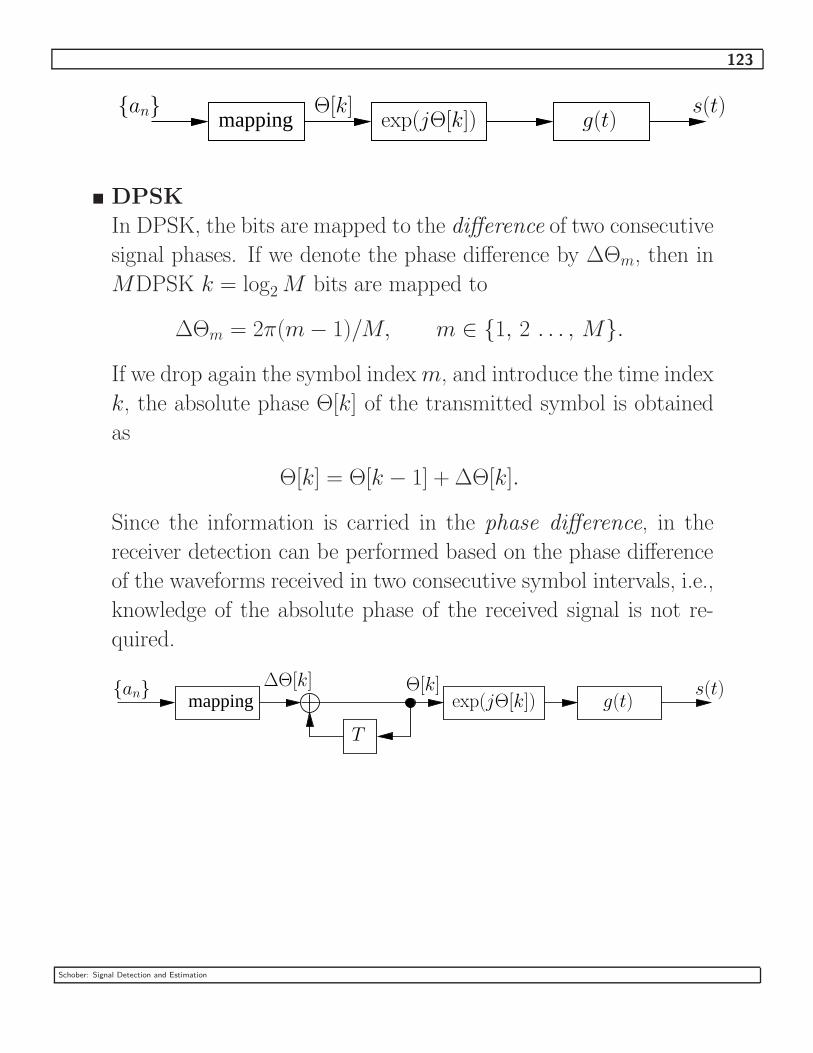
123

mapping exp(jΘ[k])s(t)

g(t){an} Θ[k]

� DPSK

In DPSK, the bits are mapped to the difference of two consecutive

signal phases. If we denote the phase difference by ∆Θm, then in

MDPSK k = log2 M bits are mapped to

∆Θm = 2π(m − 1)/M, m ∈ {1, 2 . . . , M}.

If we drop again the symbol index m, and introduce the time index

k, the absolute phase Θ[k] of the transmitted symbol is obtained

as

Θ[k] = Θ[k − 1] + ∆Θ[k].

Since the information is carried in the phase difference, in the

receiver detection can be performed based on the phase difference

of the waveforms received in two consecutive symbol intervals, i.e.,

knowledge of the absolute phase of the received signal is not re-

quired.

mapping exp(jΘ[k]){an} Θ[k]∆Θ[k]

T

s(t)g(t)


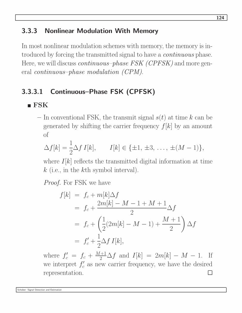
124

3.3.3 Nonlinear Modulation With Memory

In most nonlinear modulation schemes with memory, the memory is in-

troduced by forcing the transmitted signal to have a continuous phase.

Here, we will discuss continuous–phase FSK (CPFSK) and more gen-

eral continuous–phase modulation (CPM).

3.3.3.1 Continuous–Phase FSK (CPFSK)

� FSK

– In conventional FSK, the transmit signal s(t) at time k can be

generated by shifting the carrier frequency f [k] by an amount

of

∆f [k] =1

2∆f I [k], I [k] ∈ {±1, ±3, . . . , ±(M − 1)},

where I [k] reflects the transmitted digital information at time

k (i.e., in the kth symbol interval).

Proof. For FSK we have

f [k] = fc + m[k]∆f

= fc +2m[k] − M − 1 + M + 1

2∆f

= fc +

(1

2(2m[k] − M − 1) +

M + 1

2

)∆f

= f ′c +

1

2∆f I [k],

where f ′c = fc + M+1

2 ∆f and I [k] = 2m[k] − M − 1. If

we interpret f ′c as new carrier frequency, we have the desired

representation.


125

– FSK is memoryless and the abrupt switching from one fre-

quency to another in successive symbol intervals results in a

relatively broad spectrum S(f) = F{s(t)} of the transmit

signal with large side lobes.

−1T

f

S(f)

1T

– The large side lobes can be avoided by changing the carrier

frequency smoothly. The resulting signal has a continuous

phase.

� CPFSK Signal

– We first consider the PAM signal

d(t) =∞∑

k=−∞

I [k]g(t − kT ),

where I [k] ∈ {±1, ±2, . . . , ±(M − 1)} and g(t) is a rectan-

gular pulse with amplitude 1/(2T ) and duration T .

12T

t

g(t)

T


126

Clearly, the FSK signal in complex baseband representation

can be expressed as

sb(t) =

√E

Texp

(j2π∆fT

∞∑k=−∞

I [k](t − kT )g(t − kT )

),

where E denotes the energy of the signal in one symbol interval.

Since t g(t) is a discontinuous function, the phase φ(t) =

2π∆fT∑∞

k=−∞I [k](t − kT )g(t − kT ) of s(t) will jump be-

tween symbol intervals. The main idea behind CPFSK is now

to avoid this jumping of the phase by integrating over d(t).

– CPFSK Baseband Signal

The CPFSK signal in complex baseband representation is

sb(t) =

√E

Texp(j[φ(t, I) + φ0])

with information carrying carrier phase

φ(t, I) = 4πfdT

t∫

−∞

d(τ ) dτ

and the definitions

fd: peak frequency deviation

φ0: initial carrier phase

I: information sequence {I [k]}

– CPFSK Passband Signal

The CPFSK signal in passband representation is given by

s(t) =

√2E

Tcos[2πfct + φ(t, I) + φ0].


127

– Information Carrying Phase

The information carrying phase in the interval kT ≤ t ≤

(k + 1)T can be rewritten as

φ(t, I) = 4πfdT

t∫

−∞

d(τ ) dτ

= 4πfdT

t∫

−∞

∞∑n=−∞

I [n]g(τ − nT ) dτ

= 4πfdT

k−1∑n=−∞

I [n]

kT∫

−∞

g(τ − nT ) dτ

︸︷︷︸12

+4πfdTI [k]

(k+1)T∫

kT

g(τ − kT ) dτ

︸︷︷︸q(t−kT )= 1

2T(t−kT )

= 2πfdT

k−1∑n=−∞

I [n]

︸︷︷︸Θ[k]

+4πfdTI [k]q(t − kT )

= Θ[k] + 2πhI [k]q(t − kT ),

where

h = 2fdT : modulation index

Θ[k]: accumulated phase memory


128

q(t) is referred to as the phase pulse shape, and since

g(t) = dq(t)/dt

is valid, g(t) is referred to as the frequency pulse shape. The

above representation of the information carrying phase φ(t, I)

clearly illustrates that CPFSK is a modulation format with

memory.

The phase pulse shape q(t) is given by

q(t) =

0, t < 0t

2T, 0 ≤ t ≤ T

12, t > T

12

q(t)

T t

3.3.3.2 Continuous Phase Modulation (CPM)

� CPM can be viewed as a generalization of CPFSK. For CPM more

general frequency pulse shapes g(t) and consequently more general

phase pulse shapes

q(t) =

t∫

−∞

g(τ ) dτ

are used.


129

� CPM Waveform

The CPM waveform in complex baseband representation is given

by

sb(t) =

√E

Texp(j[φ(t, I) + φ0]),

whereas the corresponding passband signal is

s(t) =

√2E

Tcos[2πfct + φ(t, I) + φ0],

where the information–carrying phase in the interval kT ≤ t ≤

(k + 1)T is given by

φ(t, I) = 2πh

k∑n=−∞

I [n]q(t − nT ).

h is the modulation index.

� Properties of g(t)

– The integral over the so–called frequency pulse g(t) is always

1/2.

∞∫

0

g(τ ) dτ = q(∞) =1

2

– Full Response CPM

In full response CPM

g(t) = 0, t ≥ T.

is valid.


130

– Partial Response CPM

In partial response CPM

g(t) 6= 0, t ≥ T.

is valid.

Example:

1. CPM with rectangular frequency pulse of length L (LREC)

g(t) =

{1

2LT, 0 ≤ t ≤ LT

0, otherwise

L = 1 (CPFSK):

12

g(t) q(t)

T Tt t

12T

L = 2:

12

g(t) q(t)

2T 2Tt t

14T


131

2. CPM with raised cosine frequency pulse of length L (LRC)

g(t) =

{1

2LT

(1 − cos

(2πtLT

)), 0 ≤ t ≤ LT

0, otherwise

L = 1:

T

g(t) q(t)

t t

1T

12

T

L = 2:

1/2

t

g(t) q(t)

t2T 2T


132

3. Gaussian Minimum–Shift Keying (GMSK)

g(t) =1

T

(Q

[2πB√

ln 2

(t −

T

2

)]− Q

[2πB√

ln 2

(t +

T

2

)])

with the Q–function

Q(x) =1

√2π

∞∫

x

e−t2/2 dt

BT is the normalized bandwidth parameter and represents the

−3 dB bandwidth of the GMSK impulse. Note that the GMSK

pulse duration increases with decreasing BT .

1−1 5−5

BT = 1.0

Tg(t)

t/T

BT = 0.1


133

� Phase Tree

The phase trajectories φ(t, I) of all possible input sequences

{I [k]} can be represented by a phase tree. For construction of

the tree it is assumed that the phase at a certain time t0 (usually

t0 = 0) is known. Usually, φ(0, I) = 0 is assumed.

Example:

Binary CPFSK

In the interval kT ≤ t ≤ (k + 1)T , we get

φ(t, I) = πh

k−1∑n=−∞

I [n] + 2πhI [k]q(t − kT ),

where I [k] ∈ {±1} and

q(t) =

0, t < 0

t/(2T ), 0 ≤ t ≤ T

1/2, t > T

If we assume φ(0, I) = 0, we get the following phase tree.


134

−2hπ

φ(t, I)

t

hπ

2TT

2hπ

−hπ

� Phase Trellis

The phase trellis is obtained by plotting the phase trajectories

modulo 2π. If h is furthermore given by

h =q

p,

where q and p are relatively prime integers, it can be shown that

φ(kT, I) can assume only a finite number of different values.

These values are called the (terminal) states of the trellis.


135

Example:

Full response CPM with odd q

In that case, we get

φ(kT, I) = πh

k∑n=−∞

I [n]

= πq

p{0, ±1, ±2, . . .}.

From the above equation we conclude that φ(kT, I) mod2π can

assume only the values

ΘS =

[0,

πq

p, 2

πq

p, . . . , (2p − 1)

πq

p

]

If we further specialize this result to CPFSK with h = 12, which is

also referred to as minimum shift–keying (MSK), we get

ΘS =

[0,

π

2, π,

3π

2

]

0

−1

−1

−1+1

+1+1 −1

+1

+1

−1φ(t, I)

tT 2T

π

3π2

π2


136

Number of States

More generally, it can be shown that for general M–ary CPM the

number S of states is given by

S =

{pML−1, even q

2pML−1, odd q

The number of states is an important indicator for the receiver

complexity required for optimum detection of the corresponding

CPM scheme.

� Phase State Diagram

Yet another representation of the CPM phase results if we just

display the terminal phase states along with the possible transitions

between these states. This representation is referred to as phase

state diagram and is more compact than the trellis representation.

However, all information related to time is not contained in the

phase state diagram.

Example:

Binary CPFSK with h = 12

0

−1+1

−1

+1

−1

+1

−1+1

3π2 π

π2


137

� Minimum Shift Keying (MSK)

CPFSK with modulation index h = 12 is also referred to as MSK.

In this case, in the interval kT ≤ t ≤ (k + 1)T the signal phase

can be expressed as

φ(t, I) = Θ[k] +1

2πI [k]

(t − kT

T

)

with

Θ[k] =1

2π

i−1∑n=−∞

I [n]

Therefore, the modulated signal is given by

s(t) =

√2E

Tcos

[2πfct + Θ[k] +

1

2πI [k]

(t − kT

T

)]

=

√2E

Tcos

[2π

(fc +

1

4TI [k]

)t + Θ[k] −

1

2kπI [k]

].

Obviously, we can interpret s(t) as a sinusoid having one of two

possible frequencies. Using the definitions

f1 = fc −1

4T

f2 = fc +1

4T

we can rewrite s(t) as

si(t) =

√2E

Tcos

[2πfit + Θ[k] +

1

2kπ(−1)i−1

], i = 1, 2.

Obviously, s1(t) and s2(t) are two sinusoids that are separated by

∆f = f2 − f1 = 1/(2T ) in frequency. Since this is the minimum


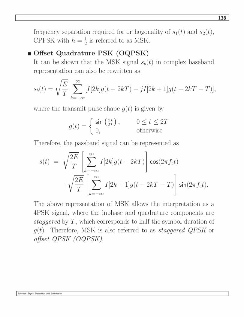
138

frequency separation required for orthogonality of s1(t) and s2(t),

CPFSK with h = 12 is referred to as MSK.

� Offset Quadrature PSK (OQPSK)

It can be shown that the MSK signal sb(t) in complex baseband

representation can also be rewritten as

sb(t) =

√E

T

∞∑k=−∞

[I [2k]g(t − 2kT ) − jI [2k + 1]g(t − 2kT − T )],

where the transmit pulse shape g(t) is given by

g(t) =

{sin(

πt2T

), 0 ≤ t ≤ 2T

0, otherwise

Therefore, the passband signal can be represented as

s(t) =

√2E

T

[∞∑

k=−∞

I [2k]g(t − 2kT )

]cos(2πfct)

+

√2E

T

[∞∑

k=−∞

I [2k + 1]g(t − 2kT − T )

]sin(2πfct).

The above representation of MSK allows the interpretation as a

4PSK signal, where the inphase and quadrature components are

staggered by T , which corresponds to half the symbol duration of

g(t). Therefore, MSK is also referred to as staggered QPSK or

offset QPSK (OQPSK).


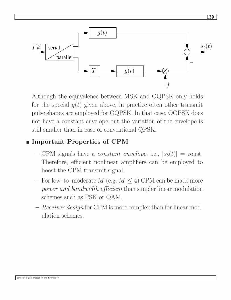
139

serial

parallel−

T

I [k]

g(t)

g(t)

j

sb(t)

Although the equivalence between MSK and OQPSK only holds

for the special g(t) given above, in practice often other transmit

pulse shapes are employed for OQPSK. In that case, OQPSK does

not have a constant envelope but the variation of the envelope is

still smaller than in case of conventional QPSK.

� Important Properties of CPM

– CPM signals have a constant envelope, i.e., |sb(t)| = const.

Therefore, efficient nonlinear amplifiers can be employed to

boost the CPM transmit signal.

– For low–to–moderate M (e.g. M ≤ 4) CPM can be made more

power and bandwidth efficient than simpler linear modulation

schemes such as PSK or QAM.

– Receiver design for CPM is more complex than for linear mod-

ulation schemes.


140

� Alternative Representations for CPM Signal

– Signal Space Representation

Because of the inherent memory, a simple description of CPM

signals in the signal space is in general not possible.

– Linear Representation

CPM signals can be described as a linear superposition of PAM

waveforms (Laurent representation, 1986).

– Representation as Trellis Encoder and Memoryless Mapper

CPM signals can also be described as a trellis encoder followed

by a memoryless mapper (Rimoldi decomposition, 1988).

Both Laurent’s and Rimoldi’s alternative representations of CPM

signals are very useful for receiver design.


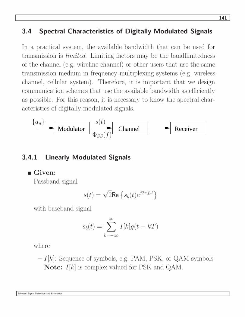
141

3.4 Spectral Characteristics of Digitally Modulated Signals

In a practical system, the available bandwidth that can be used for

transmission is limited. Limiting factors may be the bandlimitedness

of the channel (e.g. wireline channel) or other users that use the same

transmission medium in frequency multiplexing systems (e.g. wireless

channel, cellular system). Therefore, it is important that we design

communication schemes that use the available bandwidth as efficiently

as possible. For this reason, it is necessary to know the spectral char-

acteristics of digitally modulated signals.

Modulator Channel Receiver{an} s(t)

ΦSS(f)

3.4.1 Linearly Modulated Signals

� Given:

Passband signal

s(t) =√

2Re{sb(t)e

j2πfct}

with baseband signal

sb(t) =

∞∑k=−∞

I [k]g(t − kT )

where

– I [k]: Sequence of symbols, e.g. PAM, PSK, or QAM symbols

Note: I [k] is complex valued for PSK and QAM.


142

– T : Symbol duration. 1/T = R/k symbols/s is the transmis-

sion rate, where R and k denote the bit rate and the number

of bits mapped to one symbol.

– g(t): Transmit pulse shape

� Problem: Find the frequency spectrum of s(t).

� Solution:

– The spectrum ΦSS(f) of the passband signal s(t) can be ex-

pressed as

ΦSS(f) =1

2[ΦSbSb

(f − fc) + Φ∗SbSb

(−f − fc)],

where ΦSbSb(f) denotes the spectrum of the equivalent base-

band signal sb(t). We observe that ΦSS(f) can be easily de-

termined, if ΦSbSb(f) is known. Therefore, in the following, we

concentrate on the calculation of ΦSbSb(f).

– {I [k]} is a sequence of random variables, i.e., {I [k]} is a discrete–

time random process. Therefore, sb(t) is also a random process

and we have to calculate the power spectral density of sb(t),

since a spectrum in the deterministic sense does not exist.

ACF of sb(t)

φSbSb(t + τ, t) = E{s∗b(t)sb(t + τ )}

= E

{(∞∑

k=−∞

I∗[k]g∗(t − kT )

)(∞∑

k=−∞

I [k]g(t + τ − kT )

)}

=

∞∑n=−∞

∞∑k=−∞

E{I∗[k]I [n]} g∗(t − kT )g(t + τ − nT )


143

{I [k]} can be assumed to be wide–sense stationary with mean

µI = E{I [k]}

and ACF

φII [λ] = E{I∗[k]I [k + λ]}.

Therefore, the ACF of sb(t) can be simplified to

φSbSb(t + τ, t) =

∞∑n=−∞

∞∑k=−∞

φII [n − k]g∗(t − kT )g(t + τ − nT )

=

∞∑λ=−∞

φII [λ]

∞∑k=−∞

g∗(t − kT )g(t + τ − kT − λT )

From the above representation we observe that

φSbSb(t + τ + mT, t + mT ) = φSbSb

(t + τ, t),

for m ∈ {. . . , −1, 0, 1, . . .}. In addition, the mean µSb(t) is also

periodic in T

µSb(t) = E{sb(t)} = µI

∞∑k=−∞

g(t − kT ).

Since both mean µSb(t) and ACF φSbSb

(t + τ, t) are periodic, sb(t)

is a cyclostationary process with period T .


144

Average ACF of sb(t)

Since we are only interested in the average spectrum of sb(t), we

eliminate the dependence of φSbSb(t + τ, t) on t by averaging over

one period T .

φSbSb(τ ) =

1

T

T/2∫

−T/2

φSbSb(t + τ, t) dt

=

∞∑λ=−∞

φII [λ]

∞∑k=−∞

1

T

T/2∫

−T/2

g∗(t − kT ) ·

g(t + τ − kT − λT ) dt

=∞∑

λ=−∞

φII [λ]∞∑

k=−∞

1

T

T/2−kT∫

−T/2−kT

g∗(t′) ·

g(t′ + τ − λT ) dt′

=∞∑

λ=−∞

φII [λ]1

T

∞∫

−∞

g∗(t′)g(t′ + τ − λT ) dt′

Now, we introduce the deterministic ACF of g(t) as

φgg(τ ) =

∞∫

−∞

g∗(t)g(t + τ ) dt,

and obtain

φSbSb(τ ) =

1

T

∞∑λ=−∞

φII [λ]φgg(τ − λT )


145

(Average) Power Spectral Density of sb(t)

The (average) power spectral density ΦSbSb(f) of sb(t) is given by

ΦSbSb(f) = F{φSbSb

(τ )}

=

∞∫

−∞

1

T

∞∑λ=−∞

∞∫

−∞

φII [λ]g∗(t)g(t + τ − λT ) dt

e−j2πfτ dτ

=1

T

∞∑λ=−∞

φII [λ]

∞∫

−∞

g∗(t)

∞∫

−∞

g(t + τ − λT )e−j2πfτ dτ dt

=1

T

∞∑λ=−∞

φII [λ]

∞∫

−∞

g∗(t)G(f)ej2πfte−j2πfTλ dt

=1

T

∞∑λ=−∞

φII [λ]e−j2πfTλ|G(f)|2

Using the fact that the discrete–time Fourier transform of the

ACF φII [λ] is given by

ΦII(f) =

∞∑λ=−∞

φII [λ]e−j2πfTλ,

we obtain for the average power spectral density of sb(t) the elegant

expression

ΦSbSb(f) =

1

T|G(f)|2ΦII(f)

– Observe that G(f) = F{g(t)} directly influences the spectrum

ΦII(f). Therefore, the transmit pulse shape g(t) can be used


146

to shape the spectrum of sb(t), and consequently that of the

passband signal s(t).

– Notice that ΦII(f) is periodic with period 1/T .

Important Special Case

In practice, the information symbols {I [k]} are usually mutually

uncorrelated and have variance σ2I . The corresponding ACF φII [λ]

is given by

φII [λ] =

{σ2

I + |µI|2, λ = 0

|µI|2, λ 6= 0

In this case, the spectrum of I [k] can be rewritten as

ΦII(f) = σ2I + |µI|

2∞∑

λ=−∞

e−j2πfTλ

Since∑∞

λ=−∞e−j2πfTλ can be interpreted as a Fourier series rep-

resentation of 1T

∑∞

λ=−∞δ(f − λ/T ), we get

ΦII(f) = σ2I +

|µI|2

T

∞∑λ=−∞

δ

(f −

λ

T

),

we obtain for ΦSbSb(f) the expression

ΦSbSb(f) =

σ2I

T|G(f)|2 +

|µI|2

T 2

∞∑λ=−∞

∣∣∣∣G(

λ

T

)∣∣∣∣2

δ

(f −

λ

T

)

This representation of ΦSbSb(f) shows that a nonzero mean µI 6= 0

leads to Dirac–Impulses in the spectrum of sb(t), which is in general

not desirable. Therefore, in practice, nonzero mean information

sequences are preferred.


147

Example:

1. Rectangular Pulse

T

g(t)

t

A

The frequency response of g(t) is given by

G(f) = ATsin(πfT )

πfTe−jπfT

Thus, the spectrum of sb(t) is

ΦSbSb(f) = σ2

IA2T

(sin(πfT )

πfT

)2

+ A2|µI|

2δ(f)

−3 −2 −1 0 1 2 30

0.2

0.4

0.6

0.8

1

1.2

fT

ΦS

bS

b(f

)


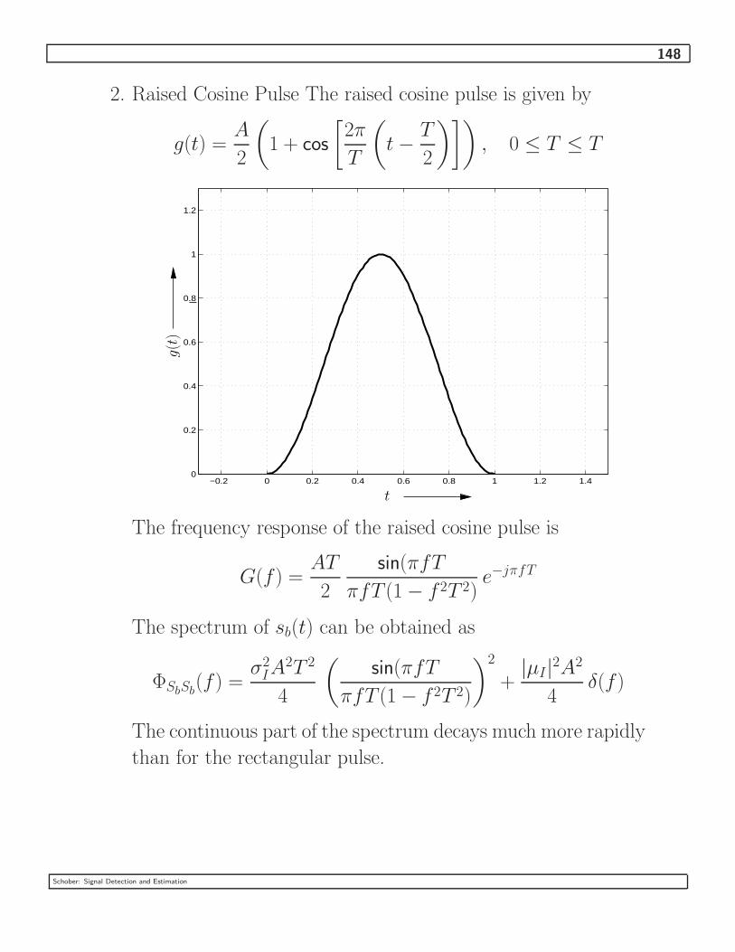
148

2. Raised Cosine Pulse The raised cosine pulse is given by

g(t) =A

2

(1 + cos

[2π

T

(t −

T

2

)]), 0 ≤ T ≤ T

−0.2 0 0.2 0.4 0.6 0.8 1 1.2 1.40

0.2

0.4

0.6

0.8

1

1.2

g(t

)

t

The frequency response of the raised cosine pulse is

G(f) =AT

2

sin(πfT

πfT (1 − f 2T 2)e−jπfT

The spectrum of sb(t) can be obtained as

ΦSbSb(f) =

σ2IA

2T 2

4

(sin(πfT

πfT (1 − f 2T 2)

)2

+|µI|

2A2

4δ(f)

The continuous part of the spectrum decays much more rapidly

than for the rectangular pulse.


149

−3 −2 −1 0 1 2 30

0.05

0.1

0.15

0.2

0.25

fT

ΦS

bS

b(f

)

−3 −2 −1 0 1 2 310

−10

10−9

10−8

10−7

10−6

10−5

10−4

10−3

10−2

10−1

fT

ΦS

bS

b(f

)


150

3.4.2 CPFSK and CPM

� In general, calculation of the power spectral density of nonlinear

modulation formats is very involved, cf. text book pp. 207–221.

Example:

Text book Figs. 4.4-3 – 4.4-10.


151

4 Optimum Reception in Additive White Gaussian

Noise (AWGN)

In this chapter, we derive the optimum receiver structures for the modu-

lation schemes introduced in Chapter 3 and analyze their performance.

4.1 Optimum Receivers for Signals Corrupted by AWGN

� Problem Formulation

– We first consider memoryless linear modulation formats. In

symbol interval 0 ≤ t ≤ T , information is transmitted using

one of M possible waveforms sm(t), 1 ≤ m ≤ M .

– The received passband signal r(t) is corrupted by real–valued

AWGN n(t):

r(t) = sm(t) + n(t), 0 ≤ t ≤ T.

n(t), N0/2

sm(t) r(t)

– The AWGN, n(t), has power spectral density

ΦNN(f) =N0

2

[W

Hz

]


152

– At the receiver, we observe r(t) and the question we ask is:

What is the best decision rule for determining sm(t)?

– This problem can be equivalently formulated in the complex

baseband. The received baseband signal rb(t) is

rb(t) = sbm(t) + z(t)

where z(t) is complex AWGN, whose real and imaginary parts

are independent. z(t) has a power spectral density of

ΦZZ(f) = N0

[W

Hz

]

z(t), N0

sbm(t) rb(t)

� Strategy: We divide the problem into two parts:

1. First we transform the received continuous–time signal r(t) (or

equivalently rb(t)) into an N–dimensional vector

r = [r1 r2 . . . rN ]T

(or rb), which forms a sufficient statistic for the detection of

sm(t) (sbm(t)). This transformation is referred to as demodu-

lation.

2. Subsequently, we determine an estimate for sm(t) (or sbm(t))

based on vector r (or rb). This process is referred to as detec-

tion.


153

DetectorDecision

Demodulatorrr(t)

4.1.1 Demodulation

The demodulator extracts the information required for optimal detec-

tion of sm(t) and eliminates those parts of the received signal r(t) that

are irrelevant for the detection process.

4.1.1.1 Correlation Demodulation

� Recall that the transmit waveforms {sm(t)} can be represented by

a set of N orthogonal basis functions fk(t), 1 ≤ k ≤ N .

� For a complete representation of the noise n(t), 0 ≤ t ≤ T , an

infinite number of basis functions are required. But fortunately,

only the noise components that lie in the signal space spanned by

fk(t), 1 ≤ k ≤ N , are relevant for detection of sm(t).

� We obtain vector r by correlating r(t) with fk(t), 1 ≤ k ≤ N

rk =

T∫

0

r(t)f∗k (t) dt =

T∫

0

[sm(t) + n(t)]f∗k (t) dt

=

T∫

0

sm(t)f∗k (t) dt

︸︷︷︸smk

+

T∫

0

n(t)f∗k (t) dt

︸︷︷︸nk

= smk + nk, 1 ≤ k ≤ N


154

... ...

rN

r(t)

∫ T

0 (·) dt

∫ T

0 (·) dt

∫ T

0 (·) dt

f∗1 (t)

f∗2 (t)

f∗N(t)

r1

r2

� r(t) can be represented by

r(t) =N∑

k=1

smkfk(t) +N∑

k=1

nkfk(t) + n′(t)

=N∑

k=1

rkfk(t) + n′(t),

where noise n′(t) is given by

n′(t) = n(t) −N∑

k=1

nkfk(t)

Since n′(t) does not lie in the signal space spanned by the basis

functions of sm(t), it is irrelevant for detection of sm(t). There-

fore, without loss of optimality, we can estimate the transmitted

waveform sm(t) from r instead of r(t).


155

� Properties of nk

– nk is a Gaussian random variable (RV), since n(t) is Gaussian.

– Mean:

E{nk} = E

T∫

0

n(t)f∗k (t) dt

=

T∫

0

E{n(t)}f∗k (t) dt

= 0

– Covariance:

E{nkn∗m} = E

T∫

0

n(t)f∗k (t) dt

T∫

0

n(t)f∗m(t) dt

∗

=

T∫

0

T∫

0

E{n(t)n∗(τ )}︸︷︷︸N02 δ(t−τ)

f∗k (t)fm(τ ) dt dτ

=N0

2

T∫

0

fm(t)f∗k (t)dt

=N0

2δ[k − m]

where δ[k] denotes the Kronecker function

δ[k] =

{1, k = 0

0, k 6= 0

We conclude that the N noise components are zero–mean, mu-

tually uncorrelated Gaussian RVs.


156

� Conditional pdf of r

r can be expressed as

r = sm + n

with

sm = [sm1 sm2 . . . smN ]T ,

n = [n1 n2 . . . nN ]T .

Therefore, conditioned on sm vector r is Gaussian distributed and

we obtain

p(r|sm) = pn(r − sm)

=N∏

k=1

pn(rk − smk),

where pn(n) and pn(nk) denote the pdfs of the Gaussian noise

vector n and the components nk of n, respectively. pn(nk) is

given by

pn(nk) =1

√πN0

exp

(−

n2k

N0

)

since nk is a real–valued Gaussian RV with variance σ2n = N0

2 .

Therefore, p(r|sm) can be expressed as

p(r|sm) =N∏

k=1

1√

πN0

exp

(−

(rk − smk)2

N0

)

=1

(πN0)N/2exp

−

N∑k=1

(rk − smk)2

N0

, 1 ≤ m ≤ M


157

p(r|sm) will be used later to find the optimum estimate for sm (or

equivalently sm(t)).

� Role of n′(t)

We consider the correlation between rk and n′(t):

E{n′(t)r∗k} = E{n′(t)(smk + nk)∗}

= E{n′(t)}︸︷︷︸=0

s∗mk + E{n′(t)n∗k}

= E

n(t) −

N∑j=1

njfj(t)

n∗

k

=

T∫

0

E{n(t)n∗(τ )}︸︷︷︸N02 δ(t−τ)

fk(τ ) dτ −

N∑j=1

E{njn∗k}︸︷︷︸

N02 δ[j−k]

fj(t)

=N0

2fk(t) −

N0

2fk(t)

= 0

We observe that r and n′(t) are uncorrelated. Since r and n′(t)

are Gaussian distributed, they are also statistically independent.

Therefore, n′(t) cannot provide any useful information that is rele-

vant for the decision, and consequently, r forms a sufficient statis-

tic for detection of sm(t).


158

4.1.1.2 Matched–Filter Demodulation

� Instead of generating the {rk} using a bank of N correlators, we

may use N linear filters instead.

� We define the N filter impulse responses hk(t) as

hk(t) = f∗k (T − t), 0 ≤ t ≤ T

where fk, 1 ≤ k ≤ N , are the N basis functions.

� The output of filter hk(t) with input r(t) is

yk(t) =

t∫

0

r(τ )hk(t − τ ) dτ

=

t∫

0

r(τ )f∗k (T − t + τ ) dτ

� By sampling yk(t) at time t = T , we obtain

yk(T ) =

T∫

0

r(τ )f∗k (τ ) dτ

= rk, 1 ≤ k ≤ N

This means the sampled output of hk(t) is rk.


159

... ...

sample at

yN(t)

r(t)

t = T

r1

r2

rN

f∗1 (T − t)

f∗2 (T − t)

f∗N(T − t)

y1(t)

y2(t)

� General Properties of Matched Filters MFs

– In general, we call a filter of the form

h(t) = s∗(T − t)

a matched filter for s(t).

– The output

y(t) =

t∫

0

s(τ )s∗(T − t + τ ) dτ

is the time–shifted time–autocorrelation of s(t).


160

Example:

s(t) h(t)

A

T t

A

T t

y(T )

y(t)

T 2T t

– MFs Maximize the SNR

∗ Consider the signal

r(t) = s(t) + n(t), 0 ≤ t ≤ T,

where s(t) is some known signal with energy

E =

T∫

0

|s(t)|2 dt

and n(t) is AWGN with power spectral density

ΦNN(f) =N0

2


161

∗ Problem: Which filter h(t) maximizes the SNR of

y(T ) = h(t) ∗ r(t)

∣∣∣∣∣t=T

∗ Answer: The matched filter h(t) = s∗(T − t)!

Proof. The filter output sampled at time t = T is given by

y(T ) =

T∫

0

r(τ )h(T − τ ) dτ

=

T∫

0

s(τ )h(T − τ ) dτ

︸︷︷︸yS(T )

+

T∫

0

n(τ )h(T − τ ) dτ

︸︷︷︸yN (T )

Now, the SNR at the filter output can be defined as

SNR =|yS(T )|2

E{|yN(T )|2}

The noise power in the denominator can be calculated as

E{|yN(T )|2

}= E

T∫

0


T∫

0


∗

=

T∫

0

T∫

0

E{n(τ )n∗(t)}︸︷︷︸N02 δ(τ−t)

h(T − τ )h∗(T − t) dτ dt

=N0

2

T∫

0

|h(T − τ )|2 dτ


162

Therefore, the SNR can be expressed as

SNR =

∣∣∣∣T∫0


∣∣∣∣2

N0

2

T∫0

|h(T − τ )|2 dτ

.

From the Cauchy–Schwartz inequality we know∣∣∣∣∣∣

T∫

0


∣∣∣∣∣∣

2

≤

T∫

0

|s(τ )|2 dτ ·

T∫

0

|h(T − τ )|2 dτ,

where equality holds if and only if

h(t) = Cs∗(T − t).

(C is an arbitrary non–zero constant). Therefore, the max-

imum output SNR is

SNR =

∣∣∣∣T∫0

|s(τ )|2 dτ

∣∣∣∣2

N0

2

T∫0

|s(τ )|2 dτ

=2

N0

T∫

0

|s(τ )|2 dτ

= 2E

N0,

which is achieved by the MF h(t) = s∗(T − t).


163

– Frequency Domain Interpretation

The frequency response of the MF is given by

H(f) = F{h(t)}

=

∞∫

−∞

s∗(T − t) e−j2πft dt

=

∞∫

−∞

s∗(τ ) ej2πfτe−j2πfT dτ

= e−j2πfT

∞∫

−∞

s(τ ) e−j2πfτ dτ

∗

= e−j2πfTS∗(f)

Observe that H(f) has the same magnitude as S(f)

|H(f)| = |S(f)|.

The factor e−j2πfT in the frequency response accounts for the

time shift of s∗(−t) by T .


164

4.1.2 Optimal Detection

Problem Formulation:

� The output r of the demodulator forms a sufficient statistic for

detection of sm(t) (sm).

� We consider linear modulation formats without memory.

� What is the optimal decision rule?

� Optimality criterion: Probability for correct detection shall be

maximized, i.e., probability of error shall be minimized.

Solution:

� The probability of error is minimized if we choose that sm which

maximizes the posteriori probability

P (sm|r), m = 1, 2, . . . , M,

where the ”tilde” indicates that sm is not the transmitted symbol

but a trial symbol.


165

Maximum a Posteriori (MAP) Decision Rule

The resulting decision rule can be formulated as

m = argmaxm

{P (sm|r)}

where m denotes the estimated signal number. The above decision

rule is called maximum a posteriori (MAP) decision rule.

� Simplifications

Using Bayes rule, we can rewrite P (sm|r) as

P (sm|r) =p(r|sm)P (sm)

p(r),

with

– p(r|sm): Conditional pdf of observed vector r given sm.

– P (sm): A priori probability of transmitted symbols. Nor-

mally, we have

P (sm) =1

M, 1 ≤ m ≤ M,

i.e., all signals of the set are transmitted with equal probability.

– p(r): Probability density function of vector r

p(r) =

M∑m=1

p(r|sm)P (sm).

Since p(r) is obviously independent of sm, we can simplify the

MAP decision rule to

m = argmaxm

{p(r|sm)P (sm)}


166

Maximum–Likelihood (ML) Decision Rule

� The MAP rule requires knowledge of both p(r|sm) and P (sm).

� In some applications P (sm) is unknown at the receiver.

� If we neglect the influence of P (sm), we get the ML decision rule

m = argmaxm

{p(r|sm)}

� Note that if all sm are equally probable, i.e., P (sm) = 1/M , 1 ≤

m ≤ M , the MAP and the ML decision rules are identical.

The above MAP and ML decision rules are very general. They can be

applied to any channel as long as we are able to find an expression for

p(r|sm).


167

ML Decision Rule for AWGN Channel

� For the AWGN channel we have

p(r|sm) =1

(πN0)N/2exp

−

N∑k=1

|rk − smk|2

N0

, 1 ≤ m ≤ M

� We note that the ML decision does not change if we maximize

ln(p(r|sm)) instead of p(r|sm) itself, since ln(·) is a monotonic

function.

� Therefore, the ML decision rule can be simplified as

m = argmaxm

{p(r|sm)}

= argmaxm

{ln(p(r|sm))}

= argmaxm

{−

N

2ln(πN0) −

1

N0

N∑k=1

|rk − smk|2

}

= argminm

{N∑

k=1

|rk − smk|2

}

= argminm

{||r − sm||

2}

� Interpretation:

We select that vector sm which has the minimum Euclidean dis-

tance

D(r, sm) = ||r − sm||


168

from the received vector r. Therefore, we can interpret the above

ML decision rule graphically by dividing the signal space in deci-

sion regions.

Example:

4QAM

r

m = 4

m = 1

m = 3

m = 2


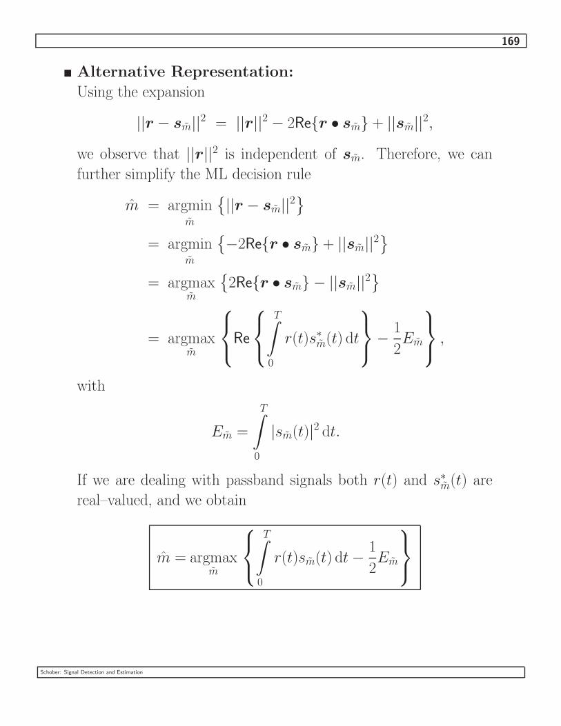
169

� Alternative Representation:

Using the expansion

||r − sm||2 = ||r||2 − 2Re{r • sm} + ||sm||

2,

we observe that ||r||2 is independent of sm. Therefore, we can

further simplify the ML decision rule

m = argminm

{||r − sm||

2}

= argminm

{−2Re{r • sm} + ||sm||

2}

= argmaxm

{2Re{r • sm} − ||sm||

2}

= argmaxm

Re

T∫

0

r(t)s∗m(t) dt

−

1

2Em

,

with

Em =

T∫

0

|sm(t)|2 dt.

If we are dealing with passband signals both r(t) and s∗m(t) are

real–valued, and we obtain

m = argmaxm

T∫

0

r(t)sm(t) dt −1

2Em


170

−

−

that

corresponds

to maximum

input

−

... ...r(t)

select m

m

12EN

12E2

12E1

s2(t)

s1(t)

sN(t)

∫ T

0 (·) dt

∫ T

0 (·) dt

∫ T

0 (·) dt

Example:

M–ary PAM transmission (baseband case)

The transmitted signals are given by

sbm(t) = Amg(t),

with Am = (2m − 1 − M)d, m = 1, 2, . . . , M , 2d: distance

between adjacent signal points.

We assume the transmit pulse g(t) is as shown below.

T

g(t)

t

a


171

In the interval 0 ≤ t ≤ T , the transmission scheme is modeled as

DetectionDemodulationsbm(t)Am

g(t)m

z(t), N0

rb

1. Demodulator

– Energy of transmit pulse

Eg =

T∫

0

|g(t)|2 dt = a2T

– Basis function f(t)

f(t) =1√Eg

g(t)

=

{1√T, 0 ≤ t ≤ T

0, otherwise


172

– Correlation demodulator

rb =

T∫

0

rb(t)f∗(t) dt

=1

√T

T∫

0

rb(t) dt

=1

√T

T∫

0

sbm(t) dt

︸︷︷︸sbm

+1

√T

T∫

0

z(t) dt

︸︷︷︸z

= sbm + z

sbm is given by

sbm =1

√T

T∫

0

Amg(t) dt

=1

√T

T∫

0

Ama dt

= a√

TAm =√

EgAm.

On the other hand, the noise variance is

σ2z = E{|z|2}

=1

T

T∫

0

T∫

0

E{z(t)z∗(τ )}︸︷︷︸N0δ(t−τ)

dt dτ

= N0


173

– pdf p(rb|Am):

p(rb|Am) =1

πN0exp

(−|rb −

√EgAm|

2

N0

)

2. Optimum Detector

The ML decision rule is given by

m = argmaxm

{ln(p(rb|Am))}

= argmaxm

{−|rb −√

EgAm|2}

= argminm

{|rb −√

EgAm|2}

Illustration in the Signal Space

m = 4m = 1 m = 2 m = 3


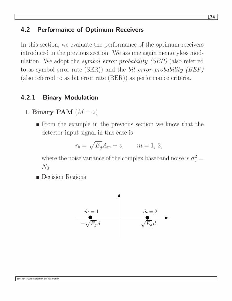
174

4.2 Performance of Optimum Receivers

In this section, we evaluate the performance of the optimum receivers

introduced in the previous section. We assume again memoryless mod-

ulation. We adopt the symbol error probability (SEP) (also referred

to as symbol error rate (SER)) and the bit error probability (BEP)

(also referred to as bit error rate (BER)) as performance criteria.

4.2.1 Binary Modulation

1. Binary PAM (M = 2)

� From the example in the previous section we know that the

detector input signal in this case is

rb =√

EgAm + z, m = 1, 2,

where the noise variance of the complex baseband noise is σ2z =

N0.

� Decision Regions

√Eg d

m = 1 m = 2

−√

Eg d


175

� Assuming s1 has been transmitted, the received signal is

rb = −√

Egd + z

and a correct decision is made if

rR < 0,

whereas an error is made if

rR > 0,

where rR = Re{rb} denotes the real part of r. rR is given by

rR = −√

Egd + zR

where zR = Re{z} is real Gaussian noise with variance σ2zR

=

N0/2.

� Consequently, the (conditional) error probability is

P (e|s1) =

∞∫

0

prR(rR|s1) drR.

Therefore, we get

P (e|s1) =

∞∫

0

1√

πN0

exp

(−

(rR − (−√

Egd))2

N0

)drR

=1

√2π

∞∫√

2EgN0

d

exp

(−

x2

2

)dx

= Q

(√2Eg

N0d

)


176

where we have used the substitution x =√

2(rR+√

Egd)/√

N0

and the Q–function is defined as

Q(x) =1

√2π

∞∫

x

exp

(−

t2

2

)dt

� The BEP, which is equal to the SEP for binary modulation, is

given by

Pb = P (s1)P (e|s1) + P (s2)P (e|s2)

For the usual case, P (s1) = P (s2) = 12, we get

Pb =1

2P (e|s1) +

1

2P (e|s2)

= P (e|s1),

since P (e|s1) = P (e|s2) is true because of the symmetry of the

signal constellation.

� In general, the BEP is expressed as a function of the received

energy per bit Eb. Here, Eb is given by

Eb = E{|√

EgAm|2}

= Eg

(1

2(−d)2 +

1

2(d)2

)

= Egd2.

Therefore, the BEP can be expressed as

Pb = Q

(√2Eb

N0

)


177

� Note that binary PSK (BPSK) yields the same BEP as 2PAM.

2. Binary Orthogonal Modulation

� For binary orthogonal modulation, the transmitted signals can

be represented as

s1 =

[ √Eb

0

]

s2 =

[0

√Eb

]

� The demodulated received signal is given by

r =

[ √Eb + n1

n2

]

and

r =

[n1√

Eb + n2

]

if s1 and s2 were sent, respectively. The noise variances are

given by

σ2n1

= E{n21} = σ2

n2= E{n2

2} =N0

2,

and n1 and n2 are mutually independent Gaussian RVs.


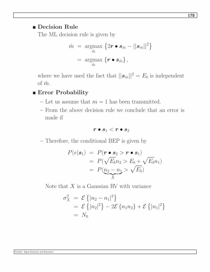
178

� Decision Rule

The ML decision rule is given by

m = argmaxm

{2r • sm − ||sm||

2}

= argmaxm

{r • sm} ,

where we have used the fact that ||sm||2 = Eb is independent

of m.

� Error Probability

– Let us assume that m = 1 has been transmitted.

– From the above decision rule we conclude that an error is

made if

r • s1 < r • s2

– Therefore, the conditional BEP is given by

P (e|s1) = P (r • s2 > r • s1)

= P (√

Ebn2 > Eb +√

Ebn1)

= P (n2 − n1︸︷︷︸X

>√

Eb)

Note that X is a Gaussian RV with variance

σ2X = E

{|n2 − n1|

2}

= E{|n2|

2}− 2E {n1n2} + E

{|n1|

2}

= N0


179

Therefore, P (e|s1) can be calculated to

P (e|s1) =1

√2πN0

∞∫√

Eb

exp

(−

x2

2N0

)dx

=1

√2π

∞∫√

EbN0

exp

(−

u2

2

)du

= Q

(√Eb

N0

)

Finally, because of the symmetry of the signal constellation

we obtain Pb = P (e|s1) = P (e|s2) or

Pb = Q

(√2Eb

N0

)


180

� Comparison of 2PAM and Binary Orthogonal Mod-

ulation

– PAM:

Pb = Q

(√2Eb

N0

)

– Orthogonal Signaling (e.g. FSK)

Pb = Q

(√Eb

N0

)

– We observe that in order to achieve the same BEP the Eb–

to–N0 ratio (SNR) has to be 3 dB higher for orthogonal sig-

naling than for PAM. Therefore, orthogonal signaling (FSK)

is less power efficient than antipodal signaling (PAM).

0 2 4 6 8 10 12 1410

−6

10−5

10−4

10−3

10−2

10−1

100

2FSK

2PAM

BE

R

Eb/N0 [dB]


181

– Signal Space

2FSK2PAM

−√

Eb

d12d12

√Eb

√Eb

√Eb

We observe that the (minimum) Euclidean distance between

signal points is given by

dPAM12 = 2

√Eb

and

dFSK12 =

√2Eb

for 2PAM and 2FSK, respectively. The ratio of the squared

Euclidean distances is given by(dPAM

12

dFSK12

)2

= 2.

Since the average energy of the signal points is identical for

both constellations, the higher power efficiency of 2PAM can

be directly deduced from the higher minimum Euclidean

distance of the signal points in the signal space. Note that

the BEP for both 2PAM and 2FSK can also be expressed

as

Pb = Q

√

d212

2N0


182

– Rule of Thumb:

In general, for a given average energy of the signal points,

the BEP of a linear modulation scheme is larger if the min-

imum Euclidean distance of the signals in the signal space

is smaller.

4.2.2 M–ary PAM

� The transmitted signal points are given by

sbm =√

EgAm, 1 ≤ m ≤ M

with pulse energy Eg and amplitude

Am = (2m − 1 − M)d, 1 ≤ m ≤ M.

� Average Energy of Signal Points

ES =1

M

M∑m=1

Em

=1

MEgd

2M∑

m=1

(2m − 1 − M)2

=Egd

2

M

[4

M∑m=1

m2

︸︷︷︸16M(M+1)(2M+1)

−4(M + 1)

M∑m=1

m

︸︷︷︸12M(M+1)

+

M∑m=1

(M + 1)2

︸︷︷︸M(M+1)2

]

=M 2 − 1

3d2Eg


183

� Received Baseband Signal

rb = sbm + z,

with σ2z = E{|z|2} = N0. Again only the real part of the received

signal is relevant for detection and we get

rR = sbm + zR,

with noise variance σ2zR

= E{z2R} = N0/2.

� Decision Regions for ML Detection

m = Mm = 1 m = 2

√Eg d

� We observe that there are two different types of signal points:

1. Outer Signal Points

We refer to the signal points with m = 1 and m = M as outer

signal points since they have only one neighboring signal point.

In this case, we make on average 1/2 symbol errors if

|rR − sbm| > d√

Eg

2. Inner Signal Points

Signal points with 2 ≤ m ≤ M − 1 are referred to as inner

signal points since they have two neighbors. Here, we make

on average 1 symbol error if |rR − sbm| > d√

Eg.


184

� Symbol Error Probability (SEP)

The SEP can be calculated to

PM =1

M

[(M − 2) +

1

2· 2

]P(|rR − sbm| > d

√Eg

)

=M − 1

MP([rR − sbm > d

√Eg] ∨ [rR − sbm < −d

√Eg])

=M − 1

M

(P(rR − sbm > d

√Eg

)+ P

(rR − sbm < −d

√Eg

))

=M − 1

M2P(rR − sbm > d

√Eg

)

= 2M − 1

M

1√

πN0

∞∫

d√

Eg

exp

(−

x2

N0

)dx

= 2M − 1

M

1√

2π

∞∫√

2d2 EgN0

exp

(−

y2

2

)dy

= 2M − 1

MQ

(√2d2

Eg

N0

)

� Using the identity

d2Eg = 3ES

M 2 − 1,

we obtain

PM = 2M − 1

MQ

(√6ES

(M 2 − 1)N0

).


185

We make the following observations

1. For constant ES the error probability increases with increasing

M .

2. For a given SEP the required ES/N0 increases as

10 log10(M2− 1) ≈ 20 log10 M.

This means if we double the number of signal points, i.e., M =

2k is increased to M = 2k+1, the required ES/N0 increases

(approximately) as

20 log10

(2k+1/2k

)= 20 log10 2 ≈ 6 dB.

� Alternatively, we may express PM as a function of the average

energy per bit Eb, which is given by

Eb =ES

k=

ES

log2 M

Therefore, the resulting expression for PM is

PM = 2M − 1

MQ

(√6 log2(M)Eb

(M 2 − 1)N0

).

� An exact expression for the bit error probability (BEP) is more

difficult to derive than the expression for the SEP. However, for

high ES/N0 ratios most errors only involve neighboring signal

points. Therefore, if we use Gray labeling we make approximately

one bit error per symbol error. Since there are log2 M bits per

symbol, the PEP can be approximated by

Pb ≈1

log2 MPM .


186

0 2 4 6 8 10 12 14 16 18 20 2210

−8

10−7

10−6

10−5

10−4

10−3

10−2

10−1

100

SE

P

M = 2

Eb/N0 [dB]

M = 32

M = 64

M = 16

M = 4 M = 8

4.2.3 M–ary PSK

� For 2PSK the same SEP as for 2PAM results.

P2 = Q

(√2Eb

N0

).

� For 4PSK the SEP is given by

P4 = 2 Q

(√2Eb

N0

)[1 −

1

2Q

(√2Eb

N0

)].

� For optimum detection of M–ary PSK the SEP can be tightly

approximated as

PM ≈ 2 Q

√

2 log2(M)Eb

N0sin

π

M

.


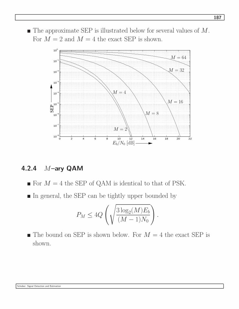
187

� The approximate SEP is illustrated below for several values of M .

For M = 2 and M = 4 the exact SEP is shown.

0 2 4 6 8 10 12 14 16 18 20 2210

−8

10−7

10−6

10−5

10−4

10−3

10−2

10−1

100

SE

P

M = 2

M = 4

M = 8

M = 16

M = 32

M = 64

Eb/N0 [dB]

4.2.4 M–ary QAM

� For M = 4 the SEP of QAM is identical to that of PSK.

� In general, the SEP can be tightly upper bounded by

PM ≤ 4Q

(√3 log2(M)Eb

(M − 1)N0

).

� The bound on SEP is shown below. For M = 4 the exact SEP is

shown.


188

0 2 4 6 8 10 12 14 16 18 20 2210

−8

10−7

10−6

10−5

10−4

10−3

10−2

10−1

100

SE

P

M = 4

M = 16

M = 64

Eb/N0 [dB]

4.2.5 Upper Bound for Arbitrary Linear Modulation Schemes

Although exact (and complicated) expressions for the SEP and BEP of

most regular linear modulation formats exist, it is sometimes more con-

venient to employ simple bounds and approximation. In this sections,

we derive the union upper bound valid for arbitrary signal constella-

tions and a related approximation for the SEP.

� We consider an M–ary modulation scheme with M signal points

sm, 1 ≤ m ≤ M , in the signal space.

� We denote the pairwise error probability of two signal points sµ

and sν , µ 6= ν by

PEP(sµ → sν) = P (sµ transmitted, sν, detected)

� The union bound for the SEP can be expressed as


189

PM ≤1

M

M∑µ=1

M∑ν=1ν 6=µ

PEP(sµ → sν)

which is an upper bound since some regions of the signal space

may be included in multiple PEPs.

� The advantage of the union bound is that the PEP can be usu-

ally easily obtained. Assuming Gaussian noise and an Euclidean

distance of dµν = ||sµ − sν|| between signal points sµ and sν , we

obtain

PM ≤1

M

M∑µ=1

M∑ν=1ν 6=µ

Q

√

d2µν

2N0

� Assuming that each signal point has on average CM nearest neigh-

bor signal points with minimum distance dmin = minµ 6=ν{dµν} and

exploiting the fact that for high SNR the minimum distance terms

will dominate the union bound, we obtain the approximation

PM ≈ CMQ

√

d2min

2N0

Note: The SEP approximation given above for MPSK can be

obtained with this approximation.

� For Gray labeling, approximations for the BEP are obtained from

the above equations with Pb ≈ PM/ log2(M)


190

4.2.6 Comparison of Different Linear Modulations

We compare PAM, PSK, and QAM for different M .

� M = 4

0 2 4 6 8 10 12 14 1610

−8

10−7

10−6

10−5

10−4

10−3

10−2

10−1

100

SE

P

4PAM

4PSK4QAM

Eb/N0 [dB]


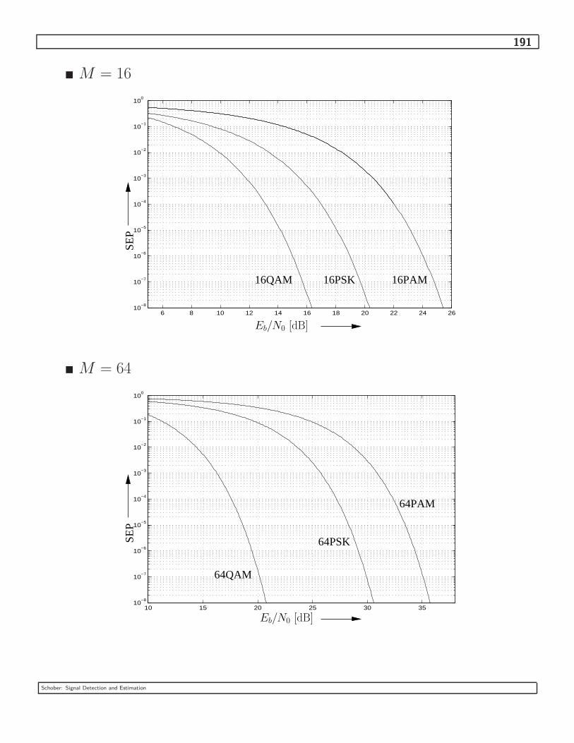
191

� M = 16

6 8 10 12 14 16 18 20 22 24 2610

−8

10−7

10−6

10−5

10−4

10−3

10−2

10−1

100

SE

P

16PAM16PSK16QAM

Eb/N0 [dB]

� M = 64

10 15 20 25 30 3510

−8

10−7

10−6

10−5

10−4

10−3

10−2

10−1

100

SE

P

64QAM

64PAM

64PSK

Eb/N0 [dB]


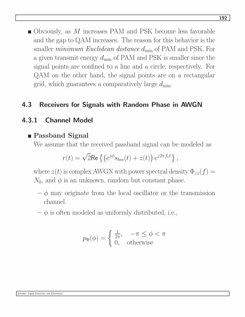
192

� Obviously, as M increases PAM and PSK become less favorable

and the gap to QAM increases. The reason for this behavior is the

smaller minimum Euclidean distance dmin of PAM and PSK. For

a given transmit energy dmin of PAM and PSK is smaller since the

signal points are confined to a line and a circle, respectively. For

QAM on the other hand, the signal points are on a rectangular

grid, which guarantees a comparatively large dmin.

4.3 Receivers for Signals with Random Phase in AWGN

4.3.1 Channel Model

� Passband Signal

We assume that the received passband signal can be modeled as

r(t) =√

2Re{(

ejφsbm(t) + z(t))ej2πfct

},

where z(t) is complex AWGN with power spectral density Φzz(f) =

N0, and φ is an unknown, random but constant phase.

– φ may originate from the local oscillator or the transmission

channel.

– φ is often modeled as uniformly distributed, i.e.,

pΦ(φ) =

{12π

, −π ≤ φ < π

0, otherwise


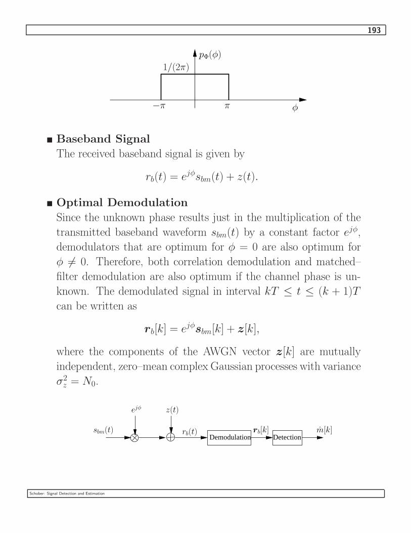
193

1/(2π)

π−π φ

pΦ(φ)

� Baseband Signal

The received baseband signal is given by

rb(t) = ejφsbm(t) + z(t).

� Optimal Demodulation

Since the unknown phase results just in the multiplication of the

transmitted baseband waveform sbm(t) by a constant factor ejφ,

demodulators that are optimum for φ = 0 are also optimum for

φ 6= 0. Therefore, both correlation demodulation and matched–

filter demodulation are also optimum if the channel phase is un-

known. The demodulated signal in interval kT ≤ t ≤ (k + 1)T

can be written as

rb[k] = ejφsbm[k] + z[k],

where the components of the AWGN vector z[k] are mutually

independent, zero–mean complex Gaussian processes with variance

σ2z = N0.

Demodulation Detectionsbm(t)

ejφ z(t)

rb(t) m[k]rb[k]


194

4.3.2 Noncoherent Detectors

In general, we distinguish between coherent and noncoherent detec-

tion.

1. Coherent Detection

� Coherent detectors first estimate the unknown phase φ using

e.g. known pilot symbols introduced into the transmitted signal

stream.

� For detection it is assumed that the phase estimate φ is perfect,

i.e., φ = φ, and the same detectors as for the pure AWGN

channel can be used.

Phase

CoherentDetection

Estimation

sbm[k]

ejφ z[k]

rb[k]

φ

e−j(·)

m[k]

� The performance of ideal coherent detection with φ = φ con-

stitutes an upper bound for any realizable non–ideal coherent

or noncoherent detection scheme.

� Disadvantages

– In practice, ideal coherent detection is not possible and the

ad hoc separation of phase estimation and detection is sub-

optimum.


195

– Phase estimation is often complicated and may require pilot

symbols.

2. Noncoherent Detection

� In noncoherent detectors no attempt is made to explicitly es-

timate the phase φ.

� Advantages

– For many modulation schemes simple noncoherent receiver

structures exist.

– More complex optimal noncoherent receivers can be de-

rived.

4.3.2.1 A Simple Noncoherent Detector for PSK with Dif-

ferential Encoding (DPSK)

� As an example for a simple, suboptimum noncoherent detector we

derive the so–called differential detector for DPSK.

� Transmit Signal

The transmitted complex baseband waveform in the interval kT ≤

t ≤ (k + 1)T is given by

sbm(t) = b[k]g(t − kT ),

where g(t) denotes the transmit pulse of length T and b[k] is the

transmitted PSK signal which is given by

b[k] = ejΘ[k].

The PSK symbols are generated from the differential PSK (DPSK)

symbols a[k] as

b[k] = a[k]b[k − 1],


196

where a[k] is given by

a[k] = ej∆Θ[k], ∆Θ[k] = 2π(m − 1)/M, m ∈ {1, 2, . . . , M}.

For simplicity, we have dropped the symbol index m in ∆Θ[k]

and a[k]. Note that the absolute phase Θ[k] is related to the

differential phase ∆Θ[k] by

Θ[k] = Θ[k − 1] + ∆Θ[k].

� For demodulation, we use the basis function

f(t) =1√Eg

g(t)

� The demodulated signal in the kth interval can be represented as

r′b[k] = ejφ√

Eg b[k] + z′[k],

where z′[k] is an AWGN process with variance σ2z′

= N0. It is

convenient to define the new signal

rb[k] =1√Eg

r′b[k]

= ejφ b[k] + z[k],

where z[k] has variance σ2z = N0/Eg.

b[k]a[k]

T

z[k]ejφ

rb[k]


197

� Differential Detection (DD)

– The received signal in the kth and the (k−1)st symbol intervals

are given by

rb[k] = ejφa[k]b[k − 1] + z[k]

and

rb[k − 1] = ejφb[k − 1] + z[k − 1],

respectively.

– If we assume z[k] ≈ 0 and z[k − 1] ≈ 0, the variable

d[k] = rb[k]r∗b [k − 1]

can be simplified to

d[k] = rb[k]r∗b [k − 1]

≈ ejφa[k]b[k − 1](ejφa[k]b[k − 1])∗

= a[k] |b[k]|2

= a[k].

This means d[k] is independent of the phase φ and is suitable

for detecting a[k].

– A detector based on d[k] is referred to as (conventional) dif-

ferential detector. The resulting decision rule is

m[k] = argminm

{|d[k] − am[k]|2

},

where am[k] = ej2π(m−1)/M , 1 ≤ m ≤ M . Alternatively, we

may base our decision on the location of d[k] in the signal space,

as usual.


198

(·)∗

rb[k] d[k] m[k]

T

� Comparison with Coherent Detection

– Coherent Detection (CD)

An upper bound on the performance of DD can be obtained

by CD with ideal knowledge of φ. In that case, we can use

the decision variable rb[k] and directly make a decision on

the absolute phase symbols b[k] = ejΘ[k] ∈ {ej2π(m−1)/M |m =

1, 2, . . . , M}.

b[k] = argminb[k]

{|b[k] − e−jφrb[k]|2

},

and obtain an estimate for the differential symbol from

am[k] = b[k] · b∗[k − 1].

b[k] and b[k] = ejΘ[k] ∈ {ej2π(m−1)/M |m = 1, 2, . . . , M} de-

note the estimated transmitted symbol and a trial symbol, re-

spectively. The above decision rule is identical to that for PSK

except for the inversion of the differential encoding operation.

T

rb[k]

e−jφ

b[k]

(·)∗

am[k]


199

Since two successive absolute symbols b[k] are necessary for

estimation of the differential symbol am[k] (or equivalently m),

isolated single errors in the absolute phase symbols will lead to

two symbol errors in the differential phase symbols, i.e., if all

absolute phase symbols but that at time k0 are correct, then all

differential phase symbols but the ones at times k0 and k0 + 1

will be correct. Since at high SNRs single errors in the absolute

phase symbols dominate, the SEP SEPCDDPSK of DPSK with CD

is approximately by a factor of two higher than that of PSK

with CD, which we refer to as SEPCDPSK.

SEPCDDPSK ≈ 2SEPCD

PSK

Note that at high SNRs this factor of two difference in SEP

corresponds to a negligible difference in required Eb/N0 ratio

to achieve a certain BER, since the SEP decays approximately

exponentially.

– Differential Detection (DD)

The decision variable d[k] can be rewritten as

d[k] = rb[k]r∗b [k − 1]

= (ejφa[k]b[k − 1] + z[k])(ejφb[k − 1] + z[k − 1])∗

= a[k] + e−jφb∗[k − 1]z[k] + ejφb[k]z∗[k − 1] + z[k]z∗[k − 1]︸︷︷︸zeff [k]

,

where zeff [k] denotes the effective noise in the decision vari-

able d[k]. It can be shown that zeff [k] is a white process with


200

variance

σ2zeff

= 2σ2z + σ4

z

= 2N0

Eg

+

(N0

Eg

)2

For high SNRs we can approximate σ2zeff

as

σ2zeff

≈ 2σ2z

= 2N0

Eg

.

– Comparison

We observe that the variance σ2zeff

of the effective noise in the

decision variable for DD is twice as high as that for CD. How-

ever, for small M the distribution of zeff [k] is significantly dif-

ferent from a Gaussian distribution. Therefore, for small M

a direct comparison of DD and CD is difficult and requires a

detailed BEP or SEP analysis. On the other hand, for large

M ≥ 8 the distribution of zeff [k] can be well approximated

as Gaussian. Therefore, we expect that at high SNRs DPSK

with DD requires approximately a 3 dB higher Eb/N0 ratio to

achieve the same BEP as CD. For M = 2 and M = 4 this dif-

ference is smaller. At a BEP of 10−5 the loss of DD compared

to CD is only about 0.8 dB and 2.3 dB for M = 2 and M = 4,

respectively.


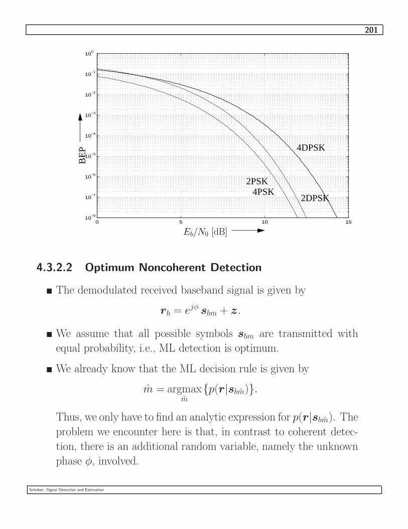
201

0 5 10 1510

−8

10−7

10−6

10−5

10−4

10−3

10−2

10−1

100

BE

P

4PSK2PSK

2DPSK

4DPSK

Eb/N0 [dB]

4.3.2.2 Optimum Noncoherent Detection

� The demodulated received baseband signal is given by

rb = ejφ sbm + z.

� We assume that all possible symbols sbm are transmitted with

equal probability, i.e., ML detection is optimum.

� We already know that the ML decision rule is given by

m = argmaxm

{p(r|sbm)}.

Thus, we only have to find an analytic expression for p(r|sbm). The

problem we encounter here is that, in contrast to coherent detec-

tion, there is an additional random variable, namely the unknown

phase φ, involved.


202

� We know the pdf of rb conditioned on both φ and sbm. It is given

by

p(rb|sbm, φ) =1

(πN0)Nexp

(−||rb − ejφ sbm||

2

N0

)

� We obtain p(rb|sbm) from p(rb|sbm, φ) as

p(rb|sbm) =

∞∫

−∞

p(rb|sbm, φ) pΦ(φ) dφ.

Since we assume for the distribution of φ

pΦ(φ) =

{12π , −π ≤ φ < π

0, otherwise

we get

p(rb|sbm) =1

2π

π∫

−π

p(rb|sbm, φ) dφ

=1

(πN0)N1

2π

π∫

−π

exp

(−||rb − ejφ sbm||

2

N0

)dφ

=1

(πN0)N1

2π

π∫

−π

exp

(−||rb||

2 + ||sbm||2 − 2Re{rb • ejφsbm}

N0

)dφ

Now, we use the relations

Re{rb • ejφsbm} = Re{|rb • sbm| ejαejφ

}

= |rb • sbm|cos(φ + α),


203

where α is the argument of rb • sbm. With this simplification

p(rb|sbm) can be rewritten as

p(rb|sbm) =1

(πN0)Nexp

(−||rb||

2 + ||sbm||2

N0

)

·1

2π

π∫

−π

exp

(2

N0|rb • sbm|cos(φ + α)

)dφ

Note that the above integral is independent of α since α is inde-

pendent of φ and we integrate over an entire period of the cosine

function. Therefore, using the definition

I0(x) =1

2π

π∫

−π

exp(xcosφ) dφ

we finally obtain

p(rb|sbm) =1

(πN0)Nexp

(−||rb||

2 + ||sbm||2

N0

)· I0

(2

N0|rb • sbm|

)


204

Note that I0(x) is the zeroth order modified Bessel function of

the first kind.

0 0.5 1 1.5 2 2.5 30

0.5

1

1.5

2

2.5

3

3.5

4

4.5

5

x

I 0(x

)

� ML Detection

With the above expression for p(rb|sbm) the noncoherent ML de-

cision rule becomes

m = argmaxm

{p(r|sbm)}.

= argmaxm

{ln[p(r|sbm)]}.

= argmaxm

{−||sbm||

2

N0+ ln

[I0

(2

N0|rb • sbm|

)]}


205

� Simplification

The above ML decision rule depends on N0, which may not be

desirable in practice, since N0 (or equivalently the SNR) has to be

estimated. However, for x ≫ 1 the approximation

ln[I0(x)] ≈ x

holds. Therefore, at high SNR (or small N0) the above ML metric

can be simplified to

m = argmaxm

{−||sbm||

2 + 2|rb • sbm|}

,

which is independent of N0. In practice, the above simplification

has a negligible impact on performance even for small arguments

(corresponding to low SNRs) of the Bessel function.

4.3.2.3 Optimum Noncoherent Detection of Binary Orthog-

onal Modulation

� Transmitted Waveform

We assume that the signal space representation of the complex

baseband transmit waveforms is

sb1 = [√

Eb 0]T

sb2 = [0√

Eb]T

� Received Signal

The corresponding demodulated received signal is

rb = [ejφ√

Eb + z1 z2]T

and

rb = [z1 ejφ√

Eb + z2]T


206

if sb1 and sb2 have been transmitted, respectively. z1 and z2 are

mutually independent complex Gaussian noise processes with iden-

tical variances σ2z = N0.

� ML Detection

For the simplification of the general ML decision rule, we exploit

the fact that for binary orthogonal modulation the relation

||sb1||2 = ||sb2||

2 = Eb

holds. The ML decision rule can be simplified as

m = argmaxm

{−||sbm||

2

N0+ ln

[I0

(2

N0|rb • sbm|

)]}

= argmaxm

{−

Eb

N0+ ln

[I0

(2

N0|rb • sbm|

)]}

= argmaxm

{ln

[I0

(2

N0|rb • sbm|

)]}

= argmaxm

{|rb • sbm|}

= argmaxm

{|rb • sbm|

2}

We decide in favor of that signal point which has a larger correla-

tion with the received signal.

� We decide for m = 1 if

|rb • sb1| > |rb • sb2|.

Using the definition

rb = [rb1 rb2]T ,


207

we obtain ∣∣∣∣[rb1

rb2

]•

[√Eb

0

]∣∣∣∣2

>

∣∣∣∣[rb1

rb2

]•

[0

√Eb

]∣∣∣∣2

|r1|2 > |r2|

2.

In other words, the ML decision rule can be simplified to

m = 1 if |r1|2 > |r2|

2

m = 2 if |r1|2 < |r2|

2

Example:

Binary FSK

– In this case, in the interval 0 ≤ t ≤ T we have

sb1(t) =

√Eb

T

sb2(t) =

√Eb

Tej2π∆ft

– If sb1(t) and sb2(t) are orthogonal, the basis functions are

f1(t) =

{1√T, 0 ≤ t ≤ T

0, otherwise

f2(t) =

{1√Tej2π∆ft, 0 ≤ t ≤ T

0, otherwise


208

– Receiver Structure

sample at

− m = 2

rb(t)

t = T

| · |2

| · |2rb1

rb2

d>

<0

f∗1 (T − t)

f∗2 (T − t)

m = 1

– If sb2(t) was transmitted, we get for rb1

rb1 =

T∫

0

rb(t)f∗1 (t) dt

=

T∫

0

ejφsb2(t)f∗1 (t) dt + z1

= ejφ 1√

T

T∫

0

sb2(t) dt + z1

=√

Ebejφ 1

T

T∫

0

ej2π∆ft dt + z1

=√

Ebejφ 1

j2π∆fTej2π∆ft

∣∣∣∣∣T

0

+ z1

=√

Ebejφ 1

j2π∆fTejπ∆fT

(ejπ∆fT

− e−jπ∆fT)

+ z1

=√

Ebej(π∆fT+φ) sinc(π∆fT ) + z1


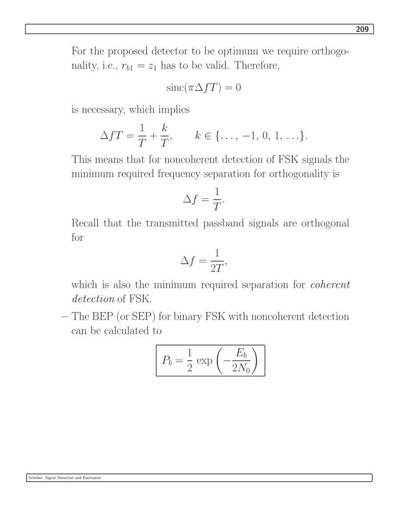
209

For the proposed detector to be optimum we require orthogo-

nality, i.e., rb1 = z1 has to be valid. Therefore,

sinc(π∆fT ) = 0

is necessary, which implies

∆fT =1

T+

k

T, k ∈ {. . . , −1, 0, 1, . . .}.

This means that for noncoherent detection of FSK signals the

minimum required frequency separation for orthogonality is

∆f =1

T.

Recall that the transmitted passband signals are orthogonal

for

∆f =1

2T,

which is also the minimum required separation for coherent

detection of FSK.

– The BEP (or SEP) for binary FSK with noncoherent detection

can be calculated to

Pb =1

2exp

(−

Eb

2N0

)


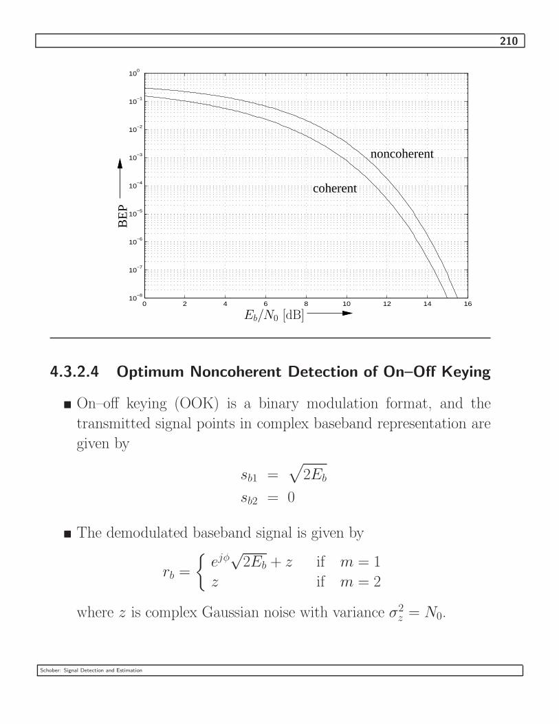
210

0 2 4 6 8 10 12 14 1610

−8

10−7

10−6

10−5

10−4

10−3

10−2

10−1

100

BE

P

coherent

noncoherent

Eb/N0 [dB]

4.3.2.4 Optimum Noncoherent Detection of On–Off Keying

� On–off keying (OOK) is a binary modulation format, and the

transmitted signal points in complex baseband representation are

given by

sb1 =√

2Eb

sb2 = 0

� The demodulated baseband signal is given by

rb =

{ejφ

√2Eb + z if m = 1

z if m = 2

where z is complex Gaussian noise with variance σ2z = N0.


211

� ML Detection

The ML decision rule is

m = argmaxm

{−|sbm|

2

N0+ ln

[I0

(2

N0|rbs

∗bm|

)]}

� We decide for m = 1 if

−2Eb

N0+ ln

[I0

(2

N0|√

2Ebrb|

)]> ln(I0(0))

ln

[I0

(2

N0

√2Eb|rb|

)]︸︷︷︸

≈2

N0

√2Eb|rb|

>2Eb

N0

|rb| >

√Eb

2

Therefore, the (approximate) ML decision rule can be simplified

to

m = 1 if |rb| >

√Eb

2

m = 2 if |rb| <

√Eb

2


212

� Signal Space Decision Regions

m = 1

m = 2

4.3.2.5 Multiple–Symbol Differential Detection (MSDD) of

DPSK

� Noncoherent detection of PSK is not possible, since for PSK the

information is represented in the absolute phase of the transmitted

signal.

� In order to enable noncoherent detection differential encoding is

necessary. The resulting scheme is referred to as differential PSK

(DPSK).


213

� The (normalized) demodulated DPSK signal in symbol interval k

is given by

rb[k] = ejφb[k] + z[k]

with b[k] = a[k]b[k − 1] and noise variance σ2z = N0/ES, where

ES denotes the received energy per DPSK symbol.

� Since the differential encoding operation introduces memory, it is

advantageous to detect the transmitted symbols in a block–wise

manner.

� In the following, we consider vectors (blocks) of length N

rb = ejφb + z,

where

rb = [rb[k] rb[k − 1] . . . rb[k − (N − 1)]T

b = [b[k] b[k − 1] . . . b[k − (N − 1)]T

z = [z[k] z[k − 1] . . . z[k − (N − 1)]T

� Since z is a Gaussian noise vector, whose components are mutu-

ally independent and have variances of σ2z = N0, respectively, the

general optimum noncoherent ML decision rule can also be applied

in this case.

� In the following, we interpret b as the transmitted baseband signal

points, i.e., sb = b, and introduce the vector of N − 1 differential

information bearing symbols

a = [a[k] a[k − 1] . . . a[k − (N − 2)]]T .

Note that the vector b of absolute phase symbols corresponds to

just the N − 1 differential symbol contained in a.


214

� The estimate for a is denoted by a, and we also introduce the

trial vectors a and b. With these definitions the ML decision rule

becomes

a = argmaxa

{−||b||2

N0+ ln

[I0

(2

N0|rb • b|

)]}

= argmaxa

{−

N

N0+ ln

[I0

(2

N0|rb • b|

)]}

= argmaxa

{|rb • b|

}

= argmaxa

{∣∣∣∣∣N−1∑ν=0

rb[k − ν]b∗[k − ν]

∣∣∣∣∣}

In order to further simplify this result we make use of the relation

b[k − ν] =N−2∏µ=ν

a[k − µ]b[k − (N − 1)]

and obtain the final ML decision rule

a = argmaxa

{∣∣∣∣∣N−1∑ν=0

rb[k − ν]N−2∏µ=ν

a∗[k − µ]b∗[k − (N − 1)]

∣∣∣∣∣}

= argmaxa

{∣∣∣∣∣N−1∑ν=0

rb[k − ν]N−2∏µ=ν

a∗[k − µ]

∣∣∣∣∣}

Note that this final result is independent of b[k − (N − 1)].

� We make a joint decision on N − 1 differential symbols a[k − ν],

0 ≤ ν ≤ N − 2, based on the observation of N received signal

points. N is also referred to as the observation window size.


215

� The above ML decision rule is known as multiple symbol differ-

ential detection (MSDD) and was reported first by Divsalar &

Simon in 1990.

� In general, the performance of MSDD increases with increasing

N . For N → ∞ the performance of ideal coherent detection is

approached.

� N = 2

For the special case N = 2, we obtain

a[k] = argmaxa[k]

{∣∣∣∣∣1∑

ν=0

rb[k − ν]

0∏µ=ν

a∗[k − µ]

∣∣∣∣∣}

= argmaxa[k]

{|rb[k]a∗[k] + rb[k − 1]|}

= argmaxa[k]

{|rb[k]a∗[k] + rb[k − 1]|2

}

= argmaxa[k]

{|rb[k]|2 + |rb[k − 1]|2 + 2Re{rb[k]a∗[k]r∗b [k − 1]}

}

= argmina[k]

{−2Re{rb[k]a∗[k]r∗b [k − 1]}}

= argmina[k]

{|rb[k]r∗b [k − 1]|2 + |a[k]|2 − 2Re{rb[k]a∗[k]r∗b [k − 1]}

}

= argmina[k]

{|d[k] − a[k]|2

}

with

d[k] = rb[k]r∗b [k − 1].

Obviously, for N = 2 the ML (MSDD) decision rule is identical to

the heuristically derived conventional differential detection decision

rule. For N > 2 the gap to coherent detection becomes smaller.


216

� Disadvantage of MSDD

The trial vector a has N − 1 elements and each element has M

possible values. Therefore, there are MN−1 different trial vectors

a. This means for MSDD we have to make MN−1/(N − 1) tests

per (scalar) symbol decision. This means the complexity of MSDD

grows exponentially with N . For example, for M = 4 we have to

make 4 and 8192 tests for N = 2 and N = 9, respectively.

� Alternatives

In order to avoid the exponential complexity of MSDD there are

two different approaches:

1. The first approach is to replace the above brute–force search

with a smarter approach. In this smarter approach the trial

vectors a are sorted first. The resulting fast decoding algorithm

still performs optimum MSDD but has only a complexity of

N log(N) (Mackenthun, 1994). For fading channels a similar

approach based on sphere decoding exists (Pauli et al.).

2. The second approach is suboptimum but achieves a similar

performance as MSDD. Complexity is reduced by using de-

cision feedback of previously decided symbols. The resulting

scheme is referred to as decision–feedback differential detection

(DF–DD). The complexity of this approach is only linear in N

(Edbauer, 1992).


217

� Comparison of BEP (BER) of MSDD (MSD) and DF–DD for

4DPSK


218

4.4 Optimum Coherent Detection of Continuous Phase Mod-

ulation (CPM)

� CPM Modulation

– CPM Transmit Signal

Recall that the CPM transmit signal in complex baseband rep-

resentation is given by

sb(t, I) =

√E

Texp(j[φ(t, I) + φ0]),

where I is the sequence {I [k]} of information bearing symbols

I [k] ∈ {±1, ±3, . . . , ±(M − 1)}, φ(t, I) is the information

carrying phase, and φ0 is the initial carrier phase. Without

loss of generality, we assume φ0 = 0 in the following.

– Information Carrying Phase

In the interval kT ≤ t ≤ (k + 1)T the phase φ(t, I) can be

written as

φ(t, I) = Θ[k] + 2πh

L−1∑ν=1

I [k − ν]q(t − [k − ν]T )

+2πhI [k]q(t − kT ),

where Θ[k] represents the accumulated phase up to time kT , h

is the so–called modulation index, and q(t) is the phase shaping

pulse with

q(t) =

0, t < 0

monotonic, 0 ≤ t ≤ LT

1/2, t > LT


219

– Trellis Diagram

If h = q/p is a rational number with relative prime integers

q and p, CPM can be described by a trellis diagram whose

number of states S is given by

S =

{pML−1, even q

2pML−1, odd q

� Received Signal

The received complex baseband signal is given by

rb(t) = sb(t, I) + z(t)

with complex AWGN z(t), which has a power spectral density of

ΦZZ(f) = N0.

� ML Detection

– Since the CPM signal has memory, ideally we have to observe

the entire received signal rb(t), −∞ ≤ t ≤ ∞, in order to

make a decision on any I [k] in the sequence of transmitted

signals.

– The conditional pdf p(rb(t)|sb(t, I)) is given by

p(rb(t)|sb(t, I)) ∝ exp

−

1

N0

∞∫

−∞

|rb(t) − sb(t, I)|2 dt

,

where I ∈ {±1, ±3, . . . , ±(M − 1)} is a trial sequence. For


220

ML detection we have the decision rule

I = argmaxI

{p(rb(t)|sb(t, I))

}

= argmaxI

{ln[p(rb(t)|sb(t, I))]

}

= argmaxI

−

∞∫

−∞

|rb(t) − sb(t, I)|2 dt

= argmaxI

−

∞∫

−∞

|rb(t)|2 dt −

∞∫

−∞

|sb(t, I)|2 dt

+

∞∫

−∞

2Re{rb(t)s∗b(t, I)} dt

= argmaxI

∞∫

−∞

Re{rb(t)s∗b(t, I)} dt,

where I refers to the ML decision. If I is a sequence of length

K, there are MK different sequences I. Since we have to cal-

culate the function∫∞

−∞Re{rb(t)s

∗b(t, I)} dt for each of these

sequences, the complexity of ML detection with brute–force

search grows exponentially with the sequence length K, which

is prohibitive for a practical implementation.


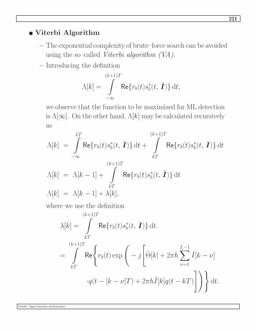
221

� Viterbi Algorithm

– The exponential complexity of brute–force search can be avoided

using the so–called Viterbi algorithm (VA).

– Introducing the definition

Λ[k] =

(k+1)T∫

−∞

Re{rb(t)s∗b(t, I)} dt,

we observe that the function to be maximized for ML detection

is Λ[∞]. On the other hand, Λ[k] may be calculated recursively

as

Λ[k] =

kT∫

−∞

Re{rb(t)s∗b(t, I)} dt +

(k+1)T∫

kT

Re{rb(t)s∗b(t, I)} dt

Λ[k] = Λ[k − 1] +

(k+1)T∫

kT

Re{rb(t)s∗b(t, I)} dt

Λ[k] = Λ[k − 1] + λ[k],

where we use the definition

λ[k] =

(k+1)T∫

kT

Re{rb(t)s∗b(t, I)} dt.

=

(k+1)T∫

kT

Re

{rb(t) exp

(− j

[Θ[k] + 2πh

L−1∑ν=1

I [k − ν]

·q(t − [k − ν]T ) + 2πhI [k]q(t − kT )

])}dt.


222

Λ[k] and λ[k] are referred to as the accumulated metric and

the branch metric of the VA, respectively.

– Since CPM can be described by a trellis with a finite number

of states S = pML−1 (S = 2pML−1), at time kT we have to

consider only S different Λ[S[k − 1], k − 1]. Each Λ[S[k −

1], k − 1] corresponds to exactly one state S[k − 1] which is

defined by

S[k − 1] = [Θ[k − 1], I [k − (L − 1)], . . . , I [k − 1]].

1

2

3

4

S[k]S[k − 2] S[k − 1]

For the interval kT ≤ t ≤ (k + 1)T we have to calculate

M branch metrics λ[S[k − 1], I [k], k] for each state S[k − 1]

corresponding to the M different I [k]. Then at time (k + 1)T

the new states are defined by

S[k] = [Θ[k], I [k − (L − 2)], . . . , I [k]],

with Θ[k] = Θ[k− 1] +πhI [k− (L− 1)]. M branches defined

by S[k− 1] and I [k] emanate in each state S[k]. We calculate


223

the M accumulated metrics

Λ[S[k − 1], I [k], k] = Λ[S[k − 1], k − 1] + λ[S[k − 1], I [k], k]

for each state S[k].

1

2

3

4

S[k]S[k − 2] S[k − 1]

From all the paths (partial sequences) that emanate in a state,

we have to retain only that one with the largest accumulated

metric denoted by

Λ[S[k], k] = maxI[k]

{Λ[S[k − 1], I [k], k]

},

since any other path with a smaller accumulated metric at time

(k +1)T cannot have a larger metric Λ[∞]. Therefore, at time

(k + 1)T there will be again only S so–called surviving paths

with corresponding accumulated metrics.


224

1

2

3

4

S[k]S[k − 2] S[k − 1]

– The above steps are carried out for all symbol intervals and at

the end of the transmission, a decision is made on the trans-

mitted sequence. Alternatively, at time kT we may use the

symbol I [k− k0] corresponding to the surviving path with the

largest accumulated metric as estimate for I [k − k0]. It has

been shown that as long as the decision delay k0 is large enough

(e.g. k0 ≥ 5 log2(S)), this method yields the same performance

as true ML detection.

– The complexity of the VA is exponential in the number of

states, but only linear in the length of the transmitted se-

quence.

� Remarks:

– At the expense of a certain loss in performance the complexity

of the VA can be further reduced by reducing the number of

states.

– Alternative implementations receivers for CPM are based on

Laurent’s decomposition of the CPM signal into a sum of PAM

signals


225

5 Signal Design for Bandlimited Channels

� So far, we have not imposed any bandwidth constraints on the

transmitted passband signal, or equivalently, on the transmitted

baseband signal

sb(t) =∞∑

k=−∞

I [k]gT (t − kT ),

where we assume a linear modulation (PAM, PSK, or QAM), and

I [k] and gT (t) denote the transmit symbols and the transmit pulse,

respectively.

� In practice, however, due to the properties of the transmission

medium (e.g. cable or multipath propagation in wireless), the un-

derlying transmission channel is bandlimited. If the bandlimited

character of the channel is not taken into account in the signal

design at the transmitter, the received signal will be (linearly) dis-

torted.

� In this chapter, we design transmit pulse shapes gT (t) that guar-

antee that sb(t) occupies only a certain finite bandwidth W . At

the same time, these pulse shapes allow ML symbol–by–symbol

detection at the receiver.


226

5.1 Characterization of Bandlimited Channels

� Many communication channels can be modeled as linear filters

with (equivalent baseband) impulse response c(t) and frequency

response C(f) = F{c(t)}.

yb(t)c(t)

z(t)

sb(t)

The received signal is given by

yb(t) =

∞∫

−∞

sb(τ )c(t − τ ) dτ + z(t),

where z(t) denotes complex Gaussian noise with power spectral

density N0.

� We assume that the channel is ideally bandlimited, i.e.,

C(f) = 0, |f | > W.

−W f

C(f)

W


227

Within the interval |f | ≤ W , the channel is characterized by

C(f) = |C(f)| ejΘ(f)

with amplitude response |C(f)| and phase response Θ(f).

� If Sb(f) = F{sb(t)} is non–zero only in the interval |f | ≤ W ,

then sb(t) is not distorted if and only if

1. |C(f)| = A, i.e., the amplitude response is constant for |f | ≤

W .

2. Θ(f) = −2πfτ0, i.e., the phase response is linear in f , where

τ0 is the delay.

In this case, the received signal is given by

yb(t) = Asb(t − τ0) + z(t).

As far as sb(t) is concerned, the impulse response of the channel

can be modeled as

c(t) = Aδ(t − τ0).

If the above conditions are not fulfilled, the channel linearly dis-

torts the transmitted signal and an equalizer is necessary at the

receiver.


228

5.2 Signal Design for Bandlimited Channels

� We assume an ideal, bandlimited channel, i.e.,

C(f) =

{1, |f | ≤ W

0, |f | > W.

� The transmit signal is

sb(t) =

∞∑k=−∞

I [k]gT (t − kT ).

� In order to avoid distortion, we assume

GT (f) = F{gT (t)} = 0, |f | > W.

This implies that the received signal is given by

yb(t) =

∞∫

−∞

sb(τ )c(t − τ ) dτ + z(t)

= sb(t) + z(t)

=∞∑

k=−∞

I [k]gT (t − kT ) + z(t).

� In order to limit the noise power in the demodulated signal, yb(t)

is usually filtered with a filter gR(t). Thereby, gR(t) can be e.g. a

lowpass filter or the optimum matched filter. The filtered received

signal is

rb(t) = gR(t) ∗ yb(t)

=

∞∑k=−∞

I [k]x(t − kT ) + ν(t)


229

where ”∗” denotes convolution, and we use the definitions

x(t) = gT (t) ∗ gR(t)

=

∞∫

−∞

gT (τ )gR(t − τ ) dτ

and

ν(t) = gR(t) ∗ z(t)

gR(t)c(t)rb(t)yb(t)

z(t)

sb(t)

� Now, we sample rb(t) at times t = kT + t0, k = . . . , −1, 0, 1, . . .,

where t0 is an arbitrary delay. For simplicity, we assume t0 = 0 in

the following and obtain

rb[k] = rb(kT )

=∞∑

κ=−∞

I [κ] x(kT − κT )︸︷︷︸=x[k−κ]

+ ν(kT )︸︷︷︸=z[k]

=∞∑

κ=−∞

I [κ]x[k − κ] + z[k]


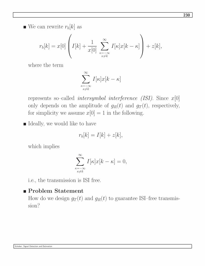
230

� We can rewrite rb[k] as

rb[k] = x[0]

I [k] +

1

x[0]

∞∑κ=−∞κ 6=k

I [κ]x[k − κ]

+ z[k],

where the term∞∑

κ=−∞κ 6=k

I [κ]x[k − κ]

represents so–called intersymbol interference (ISI). Since x[0]

only depends on the amplitude of gR(t) and gT (t), respectively,

for simplicity we assume x[0] = 1 in the following.

� Ideally, we would like to have

rb[k] = I [k] + z[k],

which implies

∞∑κ=−∞κ 6=k

I [κ]x[k − κ] = 0,

i.e., the transmission is ISI free.

� Problem Statement

How do we design gT (t) and gR(t) to guarantee ISI–free transmis-

sion?


231

� Solution: The Nyquist Criterion

– Since

x(t) = gR(t) ∗ gT (t)

is valid, the Fourier transform of x(t) can be expressed as

X(f) = GT (f) GR(f),

with GT (f) = F{gT (t)} and GR(f) = F{gR(t)}.

– For ISI–free transmission, x(t) has to have the property

x(kT ) = x[k] =

{1, k = 0

0, k 6= 0(1)

– The Nyquist Criterion

According to the Nyquist Criterion, condition (1) is fulfilled if

and only if

∞∑m=−∞

X(f +

m

T

)= T

is true. This means summing up all spectra that can be ob-

tained by shifting X(f) by multiples of 1/T results in a con-

stant.


232

Proof:

x(t) may be expressed as

x(t) =

∞∫

−∞

X(f)ej2πft df.

Therefore, x[k] = x(kT ) can be written as

x[k] =

∞∫

−∞

X(f)ej2πfkT df

=∞∑

m=−∞

(2m+1)/(2T )∫

(2m−1)/(2T )

X(f)ej2πfkT df

=∞∑

m=−∞

1/(2T )∫

−1/(2T )

X(f ′ + m/T )ej2π(f ′+m/T )kT df ′

=

1/(2T )∫

−1/(2T )

∞∑m=−∞

X(f ′ + m/T )

︸︷︷︸B(f ′)

ej2πf ′kT df ′

=

1/(2T )∫

−1/(2T )

B(f)ej2πfkT df (2)

Since

B(f) =∞∑

m=−∞

X(f + m/T )


233

is periodic with period 1/T , it can be expressed as a Fourier series

B(f) =∞∑

k=−∞

b[k]ej2πfkT (3)

where the Fourier series coefficients b[k] are given by

b[k] = T

1/(2T )∫

−1/(2T )

B(f)e−j2πfkT df. (4)

From (2) and (4) we observe that

b[k] = Tx(−kT ).

Therefore, (1) holds if and only if

b[k] =

{T, k = 0

0, k 6= 0.

However, in this case (3) yields

B(f) = T,

which means∞∑

m=−∞

X(f + m/T ) = T.

This completes the proof.

�


234

� The Nyquist criterion specifies the necessary and sufficient con-

dition that has to be fulfilled by the spectrum X(f) of x(t) for

ISI–free transmission. Pulse shapes x(t) that satisfy the Nyquist

criterion are referred to as Nyquist pulses. In the following, we

discuss three different cases for the symbol duration T . In partic-

ular, we consider T < 1/(2W ), T = 1/(2W ), and T > 1/(2W ),

respectively, where W is the bandwidth of the ideally bandlimited

channel.

1. T < 1/(2W )

If the symbol duration T is smaller than 1/(2W ), we get ob-

viously

1

2T> W

and

B(f) =∞∑

m=−∞

X(f + m/T )

consists of non–overlapping pulses.

−W

B(f)

fW 12T−

12T

We observe that in this case the condition B(f) = T cannot

be fulfilled. Therefore, ISI–free transmission is not possible.


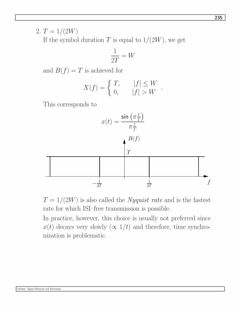
235

2. T = 1/(2W )

If the symbol duration T is equal to 1/(2W ), we get

1

2T= W

and B(f) = T is achieved for

X(f) =

{T, |f | ≤ W

0, |f | > W.

This corresponds to

x(t) =sin

(π t

T

)π t

T

12T

T

B(f)

f−1

2T

T = 1/(2W ) is also called the Nyquist rate and is the fastest

rate for which ISI–free transmission is possible.

In practice, however, this choice is usually not preferred since

x(t) decays very slowly (∝ 1/t) and therefore, time synchro-

nization is problematic.


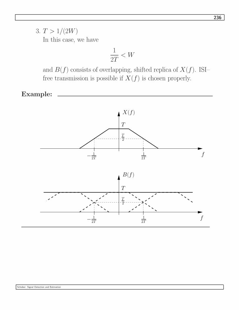
236

3. T > 1/(2W )

In this case, we have

1

2T< W

and B(f) consists of overlapping, shifted replica of X(f). ISI–

free transmission is possible if X(f) is chosen properly.

Example:

T2

T

12T

f

X(f)

−1

2T

−1

2T

T

B(f)

f

T2

12T


237

The bandwidth occupied beyond the Nyquist bandwidth 1/(2T ) is

referred to as the excess bandwidth. In practice, Nyquist pulses with

raised–cosine spectra are popular

X(f) =

T, 0 ≤ |f | ≤ 1−β2T

T2

(1 + cos

(πTβ

[|f | − 1−β

2T

])), 1−β

2T < |f | ≤ 1+β2T

0, |f | > 1+β2T

where β, 0 ≤ β ≤ 1, is the roll–off factor. The inverse Fourier trans-

form of X(f) yields

x(t) =sin(πt/T )

πt/T

cos(πβt/T )

1 − 4β2t2/T 2.

For β = 0, x(t) reduces to x(t) = sin(πt/T )/(πt/T ). For β > 0, x(t)

decays as 1/t3. This fast decay is desirable for time synchronization.

−1 −0.8 −0.6 −0.4 −0.2 0 0.2 0.4 0.6 0.8 10

0.1

0.2

0.3

0.4

0.5

0.6

0.7

0.8

0.9

1

fT

X(f

)/T

β = 0

β = 0.35

β = 1


238

−4 −3 −2 −1 0 1 2 3 4−0.4

−0.2

0

0.2

0.4

0.6

0.8

1

β = 0.35

t/T

x(t

)

β = 1

β = 0


239

�

√Nyquist–Filters

The spectrum of x(t) is given by

GT (f) GR(f) = X(f)

ISI–free transmission is of course possible for any choice of GT (f)

and GR(f) as long as X(f) fulfills the Nyquist criterion. However,

the SNR maximizing optimum choice is

GT (f) = G(f)

GR(f) = αG∗(f),

i.e., gR(t) is matched to gT (t). α is a constant. In that case, X(f)

is given by

X(f) = α|G(f)|2

and consequently, G(f) can be expressed as

G(f) =

√1

αX(f).

G(f) is referred to as√

Nyquist–Filter. In practice, a delay τ0

may be added to GT (f) and/or GR(f) to make them causal filters

in order to ensure physical realizability of the filters.


240

5.3 Discrete–Time Channel Model for ISI–free Transmission

� Continuous–Time Channel Model

gR(t)I [k]

c(t)

z(t)

kTrb[k]rb(t)

gT (t)

gT (t) and gR(t) are√

Nyquist–Impulses that are matched to each

other.

� Equivalent Discrete–Time Channel Model

√EgI [k] rb[k]

z[k]

z[k] is a discrete–time AWGN process with variance σ2Z = N0.

Proof:

– Signal Component

The overall channel is given by

x[k] = gT (t) ∗ c(t) ∗ gR(t)

∣∣∣∣∣t=kT

= gT (t) ∗ gR(t)

∣∣∣∣∣t=kT

,


241

where we have used the fact that the channel acts as an ideal

lowpass filter. We assume

gR(t) = g(t)

gT (t) =1√Eg

g∗(−t),

where g(t) is a√

Nyquist–Impulse, and Eg is given by

Eg =

∞∫

−∞

|g(t)|2 dt

Consequently, x[k] is given by

x[k] =1√Eg

g(t) ∗ g∗(−t)

∣∣∣∣∣t=kT

=1√Eg

g(t) ∗ g∗(−t)

∣∣∣∣∣t=0

δ[k]

=1√Eg

Eg δ[k]

=√

Eg δ[k]

– Noise Component

z(t) is a complex AWGN process with power spectral density


242

ΦZZ(f) = N0. z[k] is given by

z[k] = gR(t) ∗ z(t)

∣∣∣∣∣t=kT

=1√Eg

g∗(−t) ∗ z(t)

∣∣∣∣∣t=kT

=1√Eg

∞∫

−∞

z(τ )g∗(kT + τ ) dτ

∗ Mean

E{z[k]} = E

1√Eg

∞∫

−∞

z(τ )g∗(kT + τ ) dτ

=1√Eg

∞∫

−∞

E{z(τ )}g∗(kT + τ ) dτ

= 0


243

∗ ACF

φZZ [λ] = E{z[k + λ]z∗[k]}

=1

Eg

∞∫

−∞

∞∫

−∞

E{z(τ1)z∗(τ2)}︸︷︷︸

N0δ(τ1−τ2)

g∗([k + λ]T + τ1)

·g(kT + τ2) dτ1dτ2

=N0

Eg

∞∫

−∞

g∗([k + λ]T + τ1)g(kT + τ1) dτ1

=N0

Eg

Eg δ[λ]

= N0 δ[λ]

This shows that z[k] is a discrete–time AWGN process with

variance σ2Z = N0 and the proof is complete.

�

� The discrete–time, demodulated received signal can be modeled as

rb[k] =√

Eg I [k] + z[k].

� This means the demodulated signal is identical to the demodulated

signal obtained for time–limited transmit pulses (see Chapter 3

and 4). Therefore, the optimum detection strategies developed in

Chapter 4 can be also applied for finite bandwidth transmission as

long as the Nyquist criterion is fulfilled.


244

6 Equalization of Channels with ISI

� Many practical channels are bandlimited and linearly distort the

transmit signal.

� In this case, the resulting ISI channel has to be equalized for reliable

detection.

� There are many different equalization techniques. In this chapter,

we will discuss the three most important equalization schemes:

1. Maximum–Likelihood Sequence Estimation (MLSE)

2. Linear Equalization (LE)

3. Decision–Feedback Equalization (DFE)

Throughout this chapter we assume linear memoryless modula-

tions such as PAM, PSK, and QAM.


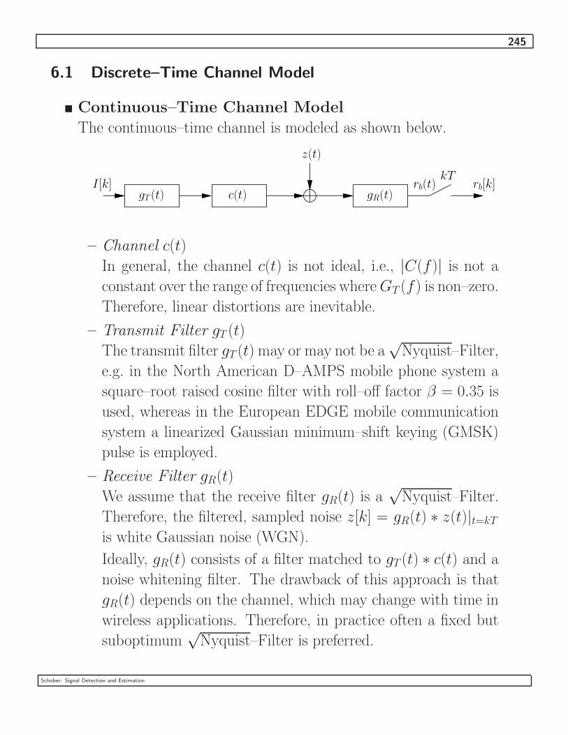
245

6.1 Discrete–Time Channel Model

� Continuous–Time Channel Model

The continuous–time channel is modeled as shown below.

gR(t)I [k]

c(t)

z(t)

kTrb[k]rb(t)

gT (t)

– Channel c(t)

In general, the channel c(t) is not ideal, i.e., |C(f)| is not a

constant over the range of frequencies where GT (f) is non–zero.

Therefore, linear distortions are inevitable.

– Transmit Filter gT (t)

The transmit filter gT (t) may or may not be a√

Nyquist–Filter,

e.g. in the North American D–AMPS mobile phone system a

square–root raised cosine filter with roll–off factor β = 0.35 is

used, whereas in the European EDGE mobile communication

system a linearized Gaussian minimum–shift keying (GMSK)

pulse is employed.

– Receive Filter gR(t)

We assume that the receive filter gR(t) is a√

Nyquist–Filter.

Therefore, the filtered, sampled noise z[k] = gR(t) ∗ z(t)|t=kT

is white Gaussian noise (WGN).

Ideally, gR(t) consists of a filter matched to gT (t) ∗ c(t) and a

noise whitening filter. The drawback of this approach is that

gR(t) depends on the channel, which may change with time in

wireless applications. Therefore, in practice often a fixed but

suboptimum√

Nyquist–Filter is preferred.


246

– Overall Channel h(t)

The overall channel impulse response h(t) is given by

h(t) = gT (t) ∗ c(t) ∗ gR(t).

� Discrete–Time Channel Model

The sampled received signal is given by

rb[k] = rb(kT )

=

(∞∑

m=−∞

I [m]h(t − mT ) + gR(t) ∗ z(t)

)∣∣∣∣∣t=kT

=

∞∑m=−∞

I [m] h(kT − mT )︸︷︷︸=h[k−m]

+ gR(t) ∗ z(t)

∣∣∣∣∣t=kT︸︷︷︸

=z[k]

=

∞∑l=−∞

h[l]I [k − l] + z[k],

where z[k] is AWGN with variance σ2Z = N0, since gR(t) is a

√Nyquist–Filter.

In practice, h[l] can be truncated to some finite length L. If we

assume causality of gT (t), gR(t), and c(t), h[l] = 0 holds for l < 0,

and if L is chosen large enough h[l] ≈ 0 holds also for l ≥ L.

Therefore, rb[k] can be rewritten as

rb[k] =

L−1∑l=0

h[l]I [k − l] + z[k]


247

I [k] h[k]

z[k]

rb[k]

For all equalization schemes derived in the following, it is assumed

that the overall channel impulse response h[k] is perfectly known,

and only the transmitted information symbols I [k] have to be es-

timated. In practice, h[k] is unknown, of course, and has to be

estimated first. However, this is not a major problem and can be

done e.g. using a training sequence of known symbols.

6.2 Maximum–Likelihood Sequence Estimation (MLSE)

� We consider the transmission of a block of K unknown information

symbols I [k], 0 ≤ k ≤ K − 1, and assume that I [k] is known for

k < 0 and k ≥ K, respectively.

� We collect the transmitted information sequence {I [k]} in a vector

I = [I [0] . . . I [K − 1]]T

and the corresponding vector of discrete–time received signals is

given by

rb = [rb[0] . . . rb[K + L − 2]]T .

Note that rb[K + L − 2] is the last received signal that contains

I [K − 1].


248

� ML Detection

For ML detection, we need the pdf p(rb|I) which is given by

p(rb|I) ∝ exp

−

1

N0

K+L−2∑k=0

∣∣∣∣∣rb[k] −

L−1∑l=0

h[l]I [k − l]

∣∣∣∣∣2 .

Consequently, the ML detection rule is given by

I = argmaxI

{p(rb|I)

}

= argmaxI

{ln[p(rb|I)]

}

= argminI

{− ln[p(rb|I)]

}

= argminI

K+L−2∑k=0

∣∣∣∣∣rb[k] −L−1∑l=0

h[l]I [k − l]

∣∣∣∣∣2 ,

where I and I denote the estimated sequence and a trial sequence,

respectively. Since the above decision rule suggest that we detect

the entire sequence I based on the received sequence rb, this op-

timal scheme is known as Maximum–Likelihood Sequence Esti-

mation (MLSE).

� Notice that there are MK different trial sequences/vectors I if M–

ary modulation is used. Therefore, the complexity of MLSE with

brute–force search is exponential in the sequence length K. This

is not acceptable for a practical implementation even for relatively

small sequence lengths. Fortunately, the exponential complexity

in K can be overcome by application of the Viterbi Algorithm

(VA).


249

� Viterbi Algorithm (VA)

For application of the VA we need to define a metric that can be

computed, recursively. Introducing the definition

Λ[k + 1] =k∑

m=0

∣∣∣∣∣rb[m] −L−1∑l=0

h[l]I [m − l]

∣∣∣∣∣2

,

we note that the function to be minimized for MLSE is Λ[K+L−1].

On the other hand,

Λ[k + 1] = Λ[k] + λ[k]

with

λ[k] =

∣∣∣∣∣rb[k] −L−1∑l=0

h[l]I [k − l]

∣∣∣∣∣2

is valid, i.e., Λ[k+1] can be calculated recursively from Λ[k], which

renders the application of the VA possible.

For M–ary modulation an ISI channel of length L can be described

by a trellis diagram with ML−1 states since the signal component

L−1∑l=0

h[l]I[k − l]

can assume ML different values that are determined by the ML−1

states

S[k] = [I [k − 1], . . . , I [k − (L − 1)]]

and the M possible transitions I [k] to state

S[k + 1] = [I [k], . . . , I [k − (L − 2)]].

Therefore, the VA operates on a trellis with ML−1 states.


250

Example:

We explain the VA more in detail using an example. We assume

BPSK transmission, i.e., I [k] ∈ {±1}, and L = 3. For k < 0 and

k ≥ K, we assume that I [k] = 1 is transmitted.

– There are ML−1 = 22 = 4 states, and M = 2 transitions per

state. State S[k] is defined as

S[k] = [I [k − 1], I [k − 2]]

– Since we know that I [k] = 1 for k < 0, state S[0] = [1, 1]

holds, whereas S[1] = [I [0], 1], and S[2] = [I [1], I [0]], and so

on. The resulting trellis is shown below.

k = 3

[1, 1]

[1,−1]

[−1, 1]

[−1,−1]

k = 0 k = 1 k = 2


251

– k = 0

Arbitrarily and without loss of optimality, we may set the ac-

cumulated metric corresponding to state S[k] at time k = 0

equal to zero

Λ(S[0], 0) = Λ([1, 1], 0) = 0.

Note that there is only one accumulated metric at time k = 0

since S[0] is known at the receiver.

– k = 1

The accumulated metric corresponding to S[1] = [I [0], 1] is

given by

Λ(S[1], 1) = Λ(S[0], 0) + λ(S[0], I [0], 0)

= λ(S[0], I [0], 0)

Since there are two possible states, namely S[1] = [1, 1] and

S[1] = [−1, 1], there are two corresponding accumulated met-

rics at time k = 1.

– k = 2

Now, there are 4 possible states S[2] = [I [1], I [0]] and for each

state a corresponding accumulated metric

Λ(S[2], 2) = Λ(S[1], 1) + λ(S[1], I [1], 1)

has to be calculated.


252

– k = 3

At k = 3 two branches emanate in each state S[3]. However,

since of the two paths that emanate in the same state S[3] that

path which has the smaller accumulated metric Λ(S[3], 3) also

will have the smaller metric at time k = K+L−2 = K+1, we

need to retain only the path with the smaller Λ(S[3], 3). This

path is also referred to as the surviving path. In mathematical

terms, the accumulated metric for state S[3] is given by

Λ(S[3], 3) = argminI[2]

{Λ(S[2], 2) + λ(S[2], I[2], 2)}

If we retain only the surviving paths, the above trellis at time

k = 3 may be as shown be below.

[−1,−1]

[1, 1]

k = 0 k = 1 k = 2 k = 3

[1,−1]

[−1, 1]

– k ≥ 4

All following steps are similar to that at time k = 3. In each

step k we retain only ML−1 = 4 surviving paths and the cor-

responding accumulated branch metrics.


253

– Termination of Trellis

Since we assume that for k ≥ K, I [k] = 1 is transmitted, the

end part of the trellis is as shown below.

[−1,−1]

[1, 1]k = K − 2 k = K − 1 k = K k = K + 1

[1,−1]

[−1, 1]

At time k = K + L − 2 = K + 1, there is only one surviving

path corresponding to the ML sequence.

� Since only ML−1 paths are retained at each step of the VA, the

complexity of the VA is linear in the sequence length K, but

exponential in the length L of the overall channel impulse response.

� If the VA is implemented as described above, a decision can be

made only at time k = K +L−2. However, the related delay may

be unacceptable for large sequence lengths K. Fortunately, empir-

ical studies have shown that the surviving paths tend to merge

relatively quickly, i.e., at time k a decision can be made on the

symbol I [k − k0] if the delay k0 is chosen large enough. In prac-

tice, k0 ≈ 5(L − 1) works well and gives almost optimum results.


254

� Disadvantage of MLSE with VA

In practice, the complexity of MLSE using the VA is often still too

high. This is especially true if M is larger than 2. For those cases

other, suboptimum equalization strategies have to be used.

� Historical Note

MLSE using the VA in the above form has been introduced by

Forney in 1972. Another variation was given later by Ungerbock

in 1974. Ungerbock’s version uses a matched filter at the receiver

but does not require noise whitening.

� Lower Bound on Performance

Exact calculation of the SEP or BEP of MLSE is quite involved and

complicated. However, a simple lower bound on the performance

of MLSE can be obtained by assuming that just one symbol I [0]

is transmitted. In that way, possibly detrimental interference from

neighboring symbols is avoided. It can be shown that the optimum

ML receiver for that scenario includes a filter matched to h[k] and

a decision can be made only based on the matched filter output at

time k = 0.

I [0]I [0]h[k]

z[k]

h∗[−k]d[0]

The decision variable d[0] is given by

d[0] =L−1∑l=0

|h[l]|2 I [0] +L−1∑l=0

h∗[−l]z[−l].


255

We can model d[0] as

d[0] = EhI [0] + z0[0],

where

Eh =

L−1∑l=0

|h[l]|2

and z0[0] is Gaussian noise with variance

σ20 = E

∣∣∣∣∣L−1∑l=0

h∗[−l]z[−l]

∣∣∣∣∣2

= Ehσ2Z = EhN0

Therefore, this corresponds to the transmission of I [0] over a non–

ISI channel with ES/N0 ratio

ES

N0=

E2h

EhN0=

Eh

N0,

and the related SEP or BEP can be calculated easily. For example,

for the BEP of BPSK we obtain

PMF = Q

(√2

Eh

N0

).

For the true BEP of MLSE we get

PMLSE ≥ PMF.

The above bound is referred to as the matched–filter (MF) bound.

The tightness of the MF bound largely depends on the underlying

channel. For example, for a channel with L = 2, h[0] = h[1] = 1


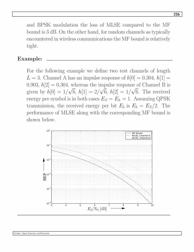
256

and BPSK modulation the loss of MLSE compared to the MF

bound is 3 dB. On the other hand, for random channels as typically

encountered in wireless communications the MF bound is relatively

tight.

Example:

For the following example we define two test channels of length

L = 3. Channel A has an impulse response of h[0] = 0.304, h[1] =

0.903, h[2] = 0.304, whereas the impulse response of Channel B is

given by h[0] = 1/√

6, h[1] = 2/√

6, h[2] = 1/√

6. The received

energy per symbol is in both cases ES = Eh = 1. Assuming QPSK

transmission, the received energy per bit Eb is Eb = ES/2. The

performance of MLSE along with the corresponding MF bound is

shown below.

3 4 5 6 7 8 9 1010

−5

10−4

10−3

10−2

10−1

100

MF BoundMLSE, Channel AMLSE, Channel B

BE

P

Eb/N0 [dB]


257

6.3 Linear Equalization (LE)

� Since MLSE becomes too complex for long channel impulse re-

sponses, in practice, often suboptimum equalizers with a lower

complexity are preferred.

� The most simple suboptimum equalizer is the so–called linear

equalizer. Roughly speaking, in LE a linear filter

F (z) = Z{f [k]}

=∞∑

k=−∞

f [k]z−k

is used to invert the channel transfer function H(z) = Z{h[k]},

and symbol–by–symbol decisions are made subsequently. f [k] de-

notes the equalizer filter coefficients.

z[k]

rb[k] d[k]I [k]I [k] H(z) F (z)

Linear equalizers are categorized with respect to the following two

criteria:

1. Optimization criterion used for calculation of the filter coef-

ficients f [k]. Here, we will adopt the so–called zero–forcing

(ZF) criterion and the minimum mean–squared error (MMSE)

criterion.

2. Finite length vs. infinite length equalization filters.


258

6.3.1 Optimum Linear Zero–Forcing (ZF) Equalization

� Optimum ZF equalization implies that we allow for equalizer filters

with infinite length impulse response (IIR).

� Zero–forcing means that it is our aim to force the residual inter-

symbol interference in the decision variable d[k] to zero.

� Since we allow for IIR equalizer filters F (z), the above goal can be

achieved by

F (z) =1

H(z)

where we assume that H(z) has no roots on the unit circle. Since

in most practical applications H(z) can be modeled as a filter with

finite impulse response (FIR), F (z) will be an IIR filter in general.

� Obviously, the resulting overall channel transfer function is

Hov(z) = H(z)F (z) = 1,

and we arrive at the equivalent channel model shown below.

I [k]d[k]

I [k]

e[k]


259

� The decision variable d[k] is given by

d[k] = I [k] + e[k]

where e[k] is colored Gaussian noise with power spectral density

Φee(ej2πfT ) = N0 |F (ej2πfT )|2

=N0

|H(ej2πfT )|2.

The corresponding error variance can be calculated to

σ2e = E{|e[k]|2}

= T

1/(2T )∫

−1/(2T )

Φee(ej2πfT ) df

= T

1/(2T )∫

−1/(2T )

N0

|H(ej2πfT )|2df.

The signal–to–noise ratio (SNR) is given by

SNRIIR−ZF =E{|I [k]|2}

σ2e

=1

T

1/(2T )∫

−1/(2T )

N0

|H(ej2πfT )|2df


260

� We may consider two extreme cases for H(z):

1. |H(ej2πfT )| =√

Eh

If H(z) has an allpass characteristic |H(ej2πfT )| =√

Eh, we

get σ2e = N0/Eh and

SNRIIR−ZF =Eh

N0.

This is the same SNR as for an undistorted AWGN channel,

i.e., no performance loss is suffered.

2. H(z) has zeros close to the unit circle.

In that case σ2e → ∞ holds and

SNRIIR−ZF → 0

follows. In this case, ZF equalization leads to a very poor per-

formance. Unfortunately, for wireless channels the probability

of zeros close to the unit circle is very high. Therefore, linear

ZF equalizers are not employed in wireless receivers.

� Error Performance

Since optimum ZF equalization results in an equivalent channel

with additive Gaussian noise, the corresponding BEP and SEP

can be easily computed. For example, for BPSK transmission we

get

PIIR−ZF = Q(√

2 SNRIIR−ZF

)


261

Example:

We consider a channel with two coefficients and energy 1

H(z) =1√

1 + |c|2(1 − cz−1),

where c is complex. The equalizer filter is given by

F (z) =√

1 + |c|2z

z − c

In the following, we consider two cases: |c| < 1 and |c| > 1.

1. |c| < 1

In this case, a stable, causal impulse response is obtained.

f [k] =√

1 + |c|2 cku[k],

where u[k] denotes the unit step function. The corresponding

error variance is

σ2e = T

1/(2T )∫

−1/(2T )

N0

|H(ej2πfT )|2df

= N0T

1/(2T )∫

−1/(2T )

|F (ej2πfT )|2 df

= N0

∞∑k=−∞

|f [k]|2

= N0(1 + |c|2)∞∑

k=0

|c|2k

= N01 + |c|2

1 − |c|2.


262

The SNR becomes

SNRIIR−ZF =1

N0

1 − |c|2

1 + |c|2.

2. |c| > 1

Now, we can realize the filter as stable and anti–causal with

impulse response

f [k] = −

√1 + |c|2

cck+1u[−(k + 1)].

Using similar techniques as above, the error variance becomes

σ2e = N0

1 + |c|2

|c|2 − 1,

and we get for the SNR

SNRIIR−ZF =1

N0

|c|2 − 1

1 + |c|2.

0 1 2 3 4 5 60

0.1

0.2

0.3

0.4

0.5

0.6

0.7

0.8

0.9

1

|c|

N0SN

RII

R−

ZF

Obviously, the SNR drops to zero as |c| approaches one, i.e., as the


263

root of H(z) approaches the unit circle.

6.3.2 ZF Equalization with FIR Filters

� In this case, we impose a causality and a length constraint on the

equalizer filter and the transfer function is given by

F (z) =

LF−1∑k=0

f [k]z−k

In order to be able to deal with ”non–causal components”, we

introduce a decision delay k0 ≥ 0, i.e., at time k, we estimate

I [k− k0]. Here, we assume a fixed value for k0, but in practice, k0

can be used for optimization.

...

...f [LF − 1]

d[k]

rb[k]

I [k − k0]

T T T

f [0] f [1]

� Because of the finite filter length, a complete elimination of ISI is

in general not possible.


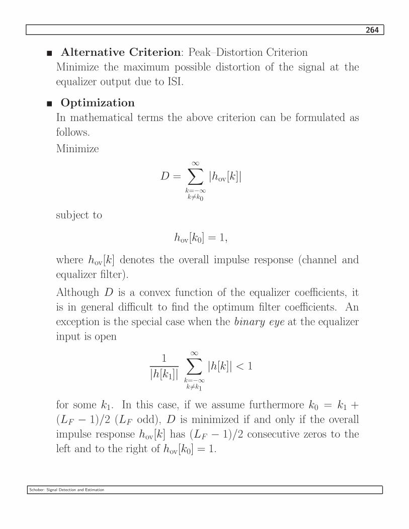
264

� Alternative Criterion: Peak–Distortion Criterion

Minimize the maximum possible distortion of the signal at the

equalizer output due to ISI.

� Optimization

In mathematical terms the above criterion can be formulated as

follows.

Minimize

D =∞∑

k=−∞k 6=k0

|hov[k]|

subject to

hov[k0] = 1,

where hov[k] denotes the overall impulse response (channel and

equalizer filter).

Although D is a convex function of the equalizer coefficients, it

is in general difficult to find the optimum filter coefficients. An

exception is the special case when the binary eye at the equalizer

input is open

1

|h[k1]|

∞∑k=−∞k 6=k1

|h[k]| < 1

for some k1. In this case, if we assume furthermore k0 = k1 +

(LF − 1)/2 (LF odd), D is minimized if and only if the overall

impulse response hov[k] has (LF − 1)/2 consecutive zeros to the

left and to the right of hov[k0] = 1.


265

k

hov[k]

LF−12

LF−12

k0

� This shows that in this special case the Peak–Distortion Criterion

corresponds to the ZF criterion for equalizers with finite order.

Note that there is no restriction imposed on the remaining coeffi-

cients of hov[k] (“don’t care positions”).

� Problem

If the binary eye at the equalizer input is closed, in general, D is

not minimized by the ZF solution. In this case, the coefficients at

the “don’t care positions” may take on large values.

� Calculation of the ZF Solution

The above ZF criterion leads us to the conditions

hov[k] =

qF∑m=0

f [m]h[k − m] = 0

where k ∈ {k0 − qF/2, . . . , k0 − 1, k0 + 1, . . . , k0 + qF/2}, and

hov[k0] =

qF∑m=0

f [m]h[k0 − m] = 1,

and qF = LF − 1. The resulting system of linear equations to be


266

solved can be written as

Hf = [0 0 . . . 0 1 0 . . . 0]T ,

with the LF × LF matrix

H =

h[k0 − qF/2] h[k0 − qF/2 − 1] · · · h[k0 − 3qF/2]

h[k0 − qF/2 + 1] h[k0 − qF/2] · · · h[k0 − 3qF/2 + 1]... ... ... ...

h[k0 − 1] h[k0 − 2] · · · h[k0 − qF − 1]

h[k0] h[k0 − 1] · · · h[k0 − qF ]

h[k0 + 1] h[k0] · · · h[k0 − qF + 1]... ... ... ...

h[k0 + qF/2] h[k0 + qF/2 − 1] · · · h[k0 − qF/2]

and coefficient vector

f = [f [0] f [1] . . . f [qF ]]T .

The ZF solution is given by

f = H−1 [0 0 . . . 0 1 0 . . . 0]T

or in other words, the optimum vector is the (qF/2 + 1)th row of

the inverse of H .

Example:

We assume

H(z) =1√

1 + |c|2(1 − cz−1),

and k0 = qF/2.


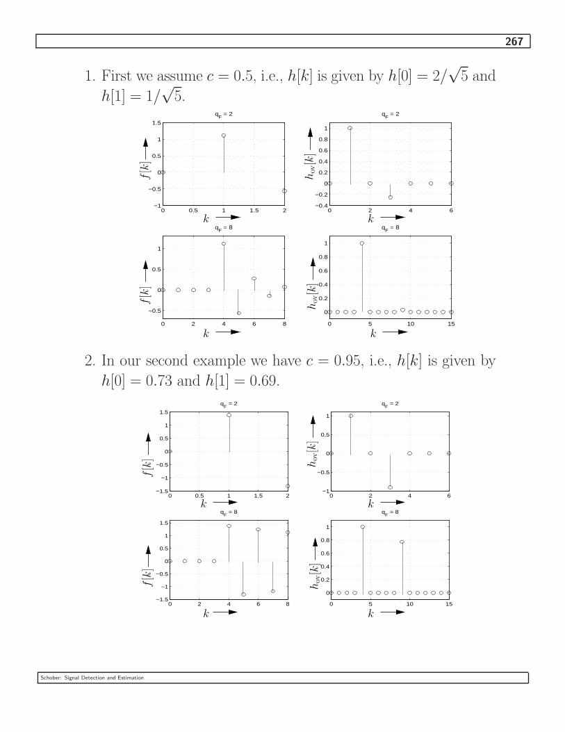
267

1. First we assume c = 0.5, i.e., h[k] is given by h[0] = 2/√

5 and

h[1] = 1/√

5.

0 0.5 1 1.5 2−1

−0.5

0

0.5

1

1.5

qF = 2

0 2 4 6−0.4

−0.2

0

0.2

0.4

0.6

0.8

1

qF = 2

0 2 4 6 8

−0.5

0

0.5

1

qF = 8

0 5 10 15

0

0.2

0.4

0.6

0.8

1

qF = 8

f[k

]f[k

]

k k

kk

hov

[k]

hov

[k]

2. In our second example we have c = 0.95, i.e., h[k] is given by

h[0] = 0.73 and h[1] = 0.69.

0 0.5 1 1.5 2−1.5

−1

−0.5

0

0.5

1

1.5

qF = 2

0 2 4 6−1

−0.5

0

0.5

1

qF = 2

0 2 4 6 8−1.5

−1

−0.5

0

0.5

1

1.5

qF = 8

0 5 10 15

0

0.2

0.4

0.6

0.8

1

qF = 8

k

k

k

k

hov

[k]

hov

[k]

f[k

]f[k

]


268

We observe that the residual interference is larger for shorter equal-

izer filter lengths and increases as the root of H(z) approaches the

unit circle.

6.3.3 Optimum Minimum Mean–Squared Error (MMSE) Equal-

ization

� Objective

Minimize the variance of the error signal

e[k] = d[k] − I [k].

z[k]

rb[k] d[k]

e[k]

I [k]I [k] H(z) F (z)

� Advantage over ZF Equalization

The MMSE criterion ensures an optimum trade–off between resid-

ual ISI in d[k] and noise enhancement. Therefore, MMSE equal-

izers achieve a significantly lower BEP compared to ZF equalizers

at low–to–moderate SNRs.


269

� Calculation of Optimum Filter F (z)

– The error signal e[k] = d[k] − I [k] depends on the estimated

symbols I [k]. Since it is very difficult to take into account the

effect of possibly erroneous decisions, for filter optimization it

is usually assumed that I [k] = I [k] is valid. The corresponding

error signal is

e[k] = d[k] − I [k].

– Cost Function

The cost function for filter optimization is given by

J = E{|e[k]|2}

= E

{(∞∑

m=−∞

f [m]rb[k − m] − I [k]

)

(∞∑

m=−∞

f∗[m]r∗b [k − m] − I∗[k]

)},

which is the error variance.

– Optimum Filter

We obtain the optimum filter coefficients from

∂J

∂f∗[κ]= E

{(∞∑

m=−∞

f [m]rb[k − m] − I [k]

)r∗b [k − κ]

}

= E {e[k]r∗b [k − κ]} = 0, κ ∈ {. . . , −1, 0, 1, . . .},

where we have used the following rules for complex differen-


270

tiation

∂f∗[κ]

∂f∗[κ]= 1

∂f [κ]

∂f∗[κ]= 0

∂|f [κ]|2

∂f∗[κ]= f [κ].

We observe that the error signal and the input of the MMSE

filter must be orthogonal. This is referred to as the orthogo-

nality principle of MMSE optimization.

The above condition can be modified to

E {e[k]r∗b [k − κ]} = E {d[k]r∗b [k − κ]} − E {I [k]r∗b [k − κ]}

The individual terms on the right hand side of the above equa-

tion can be further simplified to

E {d[k]r∗b [k − κ]} =∞∑

m=−∞

f [m] E {rb[k − m]r∗b [k − κ]}︸︷︷︸φrr[κ−m]

,

and

E {I [k]r∗b [k − κ]} =∞∑

m=−∞

h∗[m] E {I [k]I∗[k − κ − m]}︸︷︷︸φII [κ+m]

=∞∑

µ=−∞

h∗[−µ]φII [κ − µ],

respectively. Therefore, we obtain

f [k] ∗ φrr[k] = h∗[−k] ∗ φII [k],


271

and the Z–transform of this equation is

F (z)Φrr(z) = H∗(1/z∗)ΦII(z)

with

Φrr(z) =∞∑

k=−∞

φrr[k]z−k

ΦII(z) =

∞∑k=−∞

φII [k]z−k.

The optimum filter transfer function is given by

F (z) =H∗(1/z∗)ΦII(z)

Φrr(z)

Usually, we assume that the noise z[k] and the data sequence

I [k] are white processes and mutually uncorrelated. We assume

furthermore that the variance of I [k] is normalized to 1. In that

case, we get

φrr[k] = h[k] ∗ h∗[−k] ∗ φII [k] + φZZ [k]

= h[k] ∗ h∗[−k] + N0 δ[k],

and

Φrr(z) = H(z)H∗(1/z∗) + N0

ΦII(z) = 1.

The optimum MMSE filter is given by

F (z) =H∗(1/z∗)

H(z)H∗(1/z∗) + N0


272

We may consider two limiting cases.

1. N0 → 0

In this case, we obtain

F (z) =1

H(z),

i.e., in the high SNR region the MMSE solution approaches

the ZF equalizer.

2. N0 → ∞

We get

F (z) =1

N0H∗(1/z∗),

i.e., the MMSE filter approaches a discrete–time matched

filter.

� Autocorrelation of Error Sequence

The ACF of the error sequence e[k] is given by

φee[λ] = E{e[k]e∗[k − λ]}

= E {e[k](d[k − λ] − I [k − λ])∗}

= φed[λ] − φeI [λ]

φed[λ] can be simplified to

φed[λ] =∞∑

m=−∞

f∗[m] E{e[k]r∗b [k − λ − m]}︸︷︷︸=0

= 0.

This means that the error signal e[k] is also orthogonal to the

equalizer output signal d[k]. For the ACF of the error we obtain

φee[λ] = −φeI [λ]

= φII [λ] − φdI [λ].


273

� Error Variance

The error variance σ2e is given by

σ2e = φII [0] − φdI [0]

= 1 − φdI [0].

σ2e can be calculated most easily from the the power spectral den-

sity

Φee(z) = ΦII(z) − ΦdI(z)

= 1 − F (z)H(z)

= 1 −H(z)H∗(1/z∗)

H(z)H∗(1/z∗) + N0

=N0

H(z)H∗(1/z∗) + N0.

More specifically, σ2e is given by

σ2e = T

1/(2T )∫

−1/(2T )

Φee(ej2πfT ) df

or

σ2e = T

1/(2T )∫

−1/(2T )

N0

|H(ej2πfT )|2 + N0df


274

� Overall Transfer Function

The overall transfer function is given by

Hov(z) = H(z)F (z)

=H(z)H∗(1/z∗)

H(z)H∗(1/z∗) + N0

=1

1 + N0

H(z)H∗(1/z∗)

= 1 −N0

H(z)H∗(1/z∗) + N0

Obviously, Hov(z) is not a constant but depends on z, i.e., there is

residual intersymbol interference. The coefficient hov[0] is obtained

from

hov[0] = T

1/(2T )∫

−1/(2T )

Hov(ej2πfT ) df

= T

1/(2T )∫

−1/(2T )

(1 − Φee(ej2πfT )) df

= 1 − σ2e < 1.

Since hov[0] < 1 is valid, MMSE equalization is said to be biased.

� SNR

The decision variable d[k] may be rewritten as

d[k] = I [k] + e[k]

= hov[0]I [k] + e[k] + (1 − hov[0])I [k]︸︷︷︸=e′[k]

,


275

where e′[k] does not contain I [k]. Using φee[λ] = −φeI [λ] the

variance of e′[k] is given by

σ2e′ = E{|e[k]|2}

= (1 − hov[0])2 + 2(1 − hov[0])φeI [0] + σ2e

= σ4e − 2σ4

e + σ2e

= σ2e − σ4

e .

Therefore, the SNR for MMSE equalization with IIR filters is given

by

SNRIIR−MMSE =h2

ov[0]

σ2e′

=(1 − σ2

e)2

σ2e(1 − σ2

e)

which yields

SNRIIR−MMSE =1 − σ2

e

σ2e


276

Example:

We consider again the channel with one root and transfer function

H(z) =1√

1 + |c|2(1 − cz−1),

where c is a complex constant. After some straightforward manip-

ulations the error variance is given by

σ2e = E{|e[k]|2}

= T

1/(2T )∫

−1/(2T )

N0

|H(ej2πfT )|2 + N0df

=N0

1 + N0

1√1 − β2

,

where β is defined as

β =2|c|

(1 + N0)(1 + |c|2).

It is easy to check that for N0 → 0, i.e., for high SNRs σ2e ap-

proaches the error variance for linear ZF equalization.

We illustrate the SNR for two different cases.


277

1. |c| = 0.5

0 2 4 6 8 10 12 14 16 18 20−5

0

5

10

15

20MMSEZF

SN

R [d

B]

1/N0 [dB]

2. |c| = 0.95

0 2 4 6 8 10 12 14 16 18 20−15

−10

−5

0

5

10

15MMSEZF

SN

R [d

B]

1/N0 [dB]


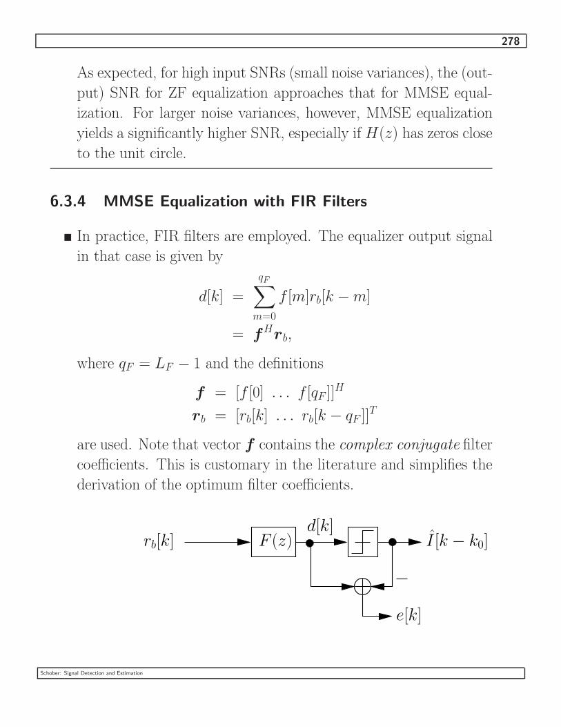
278

As expected, for high input SNRs (small noise variances), the (out-

put) SNR for ZF equalization approaches that for MMSE equal-

ization. For larger noise variances, however, MMSE equalization

yields a significantly higher SNR, especially if H(z) has zeros close

to the unit circle.

6.3.4 MMSE Equalization with FIR Filters

� In practice, FIR filters are employed. The equalizer output signal

in that case is given by

d[k] =

qF∑m=0

f [m]rb[k − m]

= fHrb,

where qF = LF − 1 and the definitions

f = [f [0] . . . f [qF ]]H

rb = [rb[k] . . . rb[k − qF ]]T

are used. Note that vector f contains the complex conjugate filter

coefficients. This is customary in the literature and simplifies the

derivation of the optimum filter coefficients.

rb[k] F (z)d[k]

I [k − k0]

e[k]


279

� Error Signal

The error signal e[k] is given by

e[k] = d[k] − I [k − k0],

where we allow for a decision delay k0 ≥ 0 to account for non–

causal components, and we assume again I [k− k0] = I [k− k0] for

the sake of mathematical tractability.

� Cost Function

The cost function for filter optimization is given by

J(f ) = E{|e[k]|2}

= E

{(fHrb − I [k − k0]

) (fHrb − I [k − k0]

)H}

= fHE{rbr

Hb }︸︷︷︸

Φrr

f − fHE{rbI

∗[k − k0]}︸︷︷︸ϕrI

−E{I [k − k0]rHb }f + E{|I [k − k0]|

2}

= fHΦrrf − fHϕrI − ϕHrIf + 1,

where Φrr denotes the autocorrelation matrix of vector rb, and

ϕrI is the crosscorrelation vector between rb and I [k− k0]. Φrr is

given by

Φrr =

φrr[0] φrr[1] · · · φrr[qF ]

φrr[−1] φrr[0] · · · φrr[qF − 1]... ... . . . ...

φrr[−qF ] φrr[−qF + 1] · · · φrr[0]

,

where φrr[λ] = E{r∗b [k]rb[k + λ]}. The crosscorrelation vector can

be calculated as

ϕrI = [φrI [k0] φrI [k0 − 1] . . . φrI [k0 − qF ]]T ,


280

where φrI [λ] = E{rb[k + λ]I∗[k]}. Note that for independent,

identically distributed input data and AWGN, we get

φrr[λ] = h[λ] ∗ h∗[−λ] + N0 δ[λ]

φrI [λ] = h[k0 + λ].

This completely specifies Φrr and ϕrI .

� Filter Optimization

The optimum filter coefficient vector can be obtained be setting

the gradient of J(f ) equal to zero

∂J(f )

∂f ∗ = 0.

For calculation of this gradient, we use the following rules for dif-

ferentiation of scalar functions with respect to (complex) vectors:

∂

∂f ∗fHXf = Xf

∂

∂f ∗fHx = x

∂

∂f ∗xHf = 0,

where X and x denote a matrix and a vector, respectively.

With these rules we obtain

∂J(f )

∂f ∗ = Φrrf − ϕrI = 0

or

Φrrf = ϕrI.


281

This equation is often referred to as the Wiener–Hopf equation.

The MMSE or Wiener solution for the optimum filter coefficients

f opt is given by

f opt = Φ−1rr ϕrI

� Error Variance

The minimum error variance is given by

σ2e = J(f opt)

= 1 − ϕHrIΦ

−1rr ϕrI

= 1 − ϕHrIf opt

� Overall Channel Coefficient hov[k0]

The coefficient hov[k0] is given by

hov[k0] = fHoptϕrI

= 1 − σ2e < 1,

i.e., also the optimum FIR MMSE filter is biased.

� SNR

Similar to the IIR case, the SNR at the output of the optimum

FIR filter can be calculated to

SNRFIR−MMSE =1 − σ2

e

σ2e


282

Example:

Below, we show f [k] and hov[k] for a channel with one root and

transfer function

H(z) =1√

1 + |c|2(1 − cz−1).

We consider the case c = 0.8 and different noise variances σ2Z = N0.

Furthermore, we use qF = 12 and k0 = 7.

0 2 4 6 8 10 12−1

−0.5

0

0.5

1

1.5

N0 = 0.2

0 5 10−0.2

0

0.2

0.4

0.6

0.8

1

N0 = 0.2

0 2 4 6 8 10 12−1

−0.5

0

0.5

1

1.5

N0 = 0.001

0 5 10−0.2

0

0.2

0.4

0.6

0.8

1

N0 = 0.001

hov

[k]

hov

[k]

k

kk

k

f[k

]f[k

]

We observe that the residual ISI in hov[k] is smaller for the smaller

noise variance, since the MMSE filter approaches the ZF filter for

N0 → 0. Also the bias decreases with decreasing noise variance,

i.e., hov[k0] approaches 1.


283

6.4 Decision–Feedback Equalization (DFE)

� Drawback of Linear Equalization

In linear equalization, the equalizer filter enhances the noise, es-

pecially in severely distorted channels with roots close to the unit

circle. The noise variance at the equalizer output is increased and

the noise is colored. In many cases, this leads to a poor perfor-

mance.

� Noise Prediction

The above described drawback of LE can be avoided by application

of linear noise prediction.

noise predictor

H(z)I [k]I [k] + e[k]

P (z)

I [k]d[k]

z[k]

1H(z)

rb[k]

e[k]T

The linear FIR noise predictor

P (z) =

LP−1∑m=0

p[m]z−m

predicts the current noise sample e[k] based on the previous LP

noise samples e[k − 1], e[k − 2], . . ., e[k −LP ]. The estimate e[k]

for e[k] is given by

e[k] =

LP−1∑m=0

p[m]e[k − 1 − m].


284

Assuming I [k − m] = I [k − m] for m ≥ 1, the new decision

variable is

d[k] = I [k] + e[k] − e[k].

If the predictor coefficients are suitably chosen, we expect that the

variance of the new error signal e[k] − e[k] is smaller than that of

e[k]. Therefore, noise prediction improves performance.

� Predictor Design

Usually an MMSE criterion is adopted for optimization of the pre-

dictor coefficients, i.e., the design objective is to minimize the error

variance

E{|e[k] − e[k]|2}.

Since this is a typical MMSE problem, the optimum predictor

coefficients can be obtained from the Wiener–Hopf equation

Φeep = ϕe

with

Φee =

φee[0] φee[1] · · · φee[LP − 1]

φee[−1] φee[0] · · · φee[LP − 2]... ... . . . ...

φee[−(LP − 1)] φee[−(LP − 2)] · · · φee[0]

,

ϕe = [φee[−1] φee[−2] . . . φee[−LP ]]T

p = [p[0] p[1] . . . p[LP − 1]]H,

where the ACF of e[k] is defined as φee[λ] = E{e∗[k]e[k + λ]}.


285

� New Block Diagram

The above block diagram of linear equalization and noise prediction

can be rearranged as follows.

feedforward filter feedback filter

H(z) 1H(z)

P (z) P (z)

I [k]I [k]

z[k]

T T

The above structure consists of two filters. A feedforward filter

whose input is the channel output signal rb[k] and a feedback filter

that feeds back previous decisions I [k − m], m ≥ 1. An equaliza-

tion scheme with this structure is referred to as decision–feedback

equalization (DFE). We have shown that the DFE structure can

be obtained in a natural way from linear equalization and noise

prediction.


286

� General DFE

If the predictor has infinite length, the above DFE scheme cor-

responds to optimum zero–forcing (ZF) DFE. However, the DFE

concept can be generalized of course allowing for different filter

optimization criteria. The structure of a general DFE scheme is

shown below.

B(z) − 1

rb[k]F (z)

d[k]I [k]I [k] H(z)

z[k]

y[k]

In general, the feedforward filter is given by

F (z) =∞∑

k=−∞

f [k]z−k,

and the feedback filter

B(z) = 1 +

LB−1∑k=1

b[k]z−k

is causal and monic (b[k] = 1). Note that F (z) may also be

an FIR filter. F (z) and B(z) can be optimized according to any

suitable criterion, e.g. ZF or MMSE criterion.


287

Typical Example:

−8 −6 −4 −2 0 2 4 6 8−0.2

0

0.2

0.4

0.6

0.8

1

0 1 2 3 4 5 6 7 8−0.2

0

0.2

0.4

0.6

0.8

1

k

k

h[k

]∗f[k

]b[

k]

� Properties of DFE

– The feedforward filter has to suppress only the pre–cursor ISI.

This imposes fewer constraints on the feedforward filter and

therefore, the noise enhancement for DFE is significantly smaller

than for linear equalization.

– The post–cursors are canceled by the feedback filter. This

causes no additional noise enhancement since the slicer elimi-

nates the noise before feedback.

– Feedback of wrong decisions causes error propagation. Fortu-


288

nately, this error propagation is usually not catastrophic but

causes some performance degradation compared to error free

feedback.

6.4.1 Optimum ZF–DFE

� Optimum ZF–DFE may be viewed as a combination of optimum

linear ZF equalization and optimum noise prediction.

P (z)

I [k] I [k]H(z) 1H(z)

z[k]

F (z)

T

B(z) − 1

TP (z)

� Equalizer Filters (I)

The feedforward filter (FFF) is the cascade of the linear equalizer

1/H(z) and the prediction error filter Pe(z) = 1 − z−1P (z)

F (z) =Pe(z)

H(z).

The feedback filter (FBF) is given by

B(z) = 1 − z−1P (z).

� Power Spectral Density of Noise

The power spectral density of the noise component e[k] is given by

Φee(z) =N0

H(z)H∗(1/z∗)


289

� Optimum Noise Prediction

The optimum noise prediction error filter is a noise whitening

filter, i.e., the power spectrum Φνν(z) of ν[k] = e[k] − e[k] is a

constant

Φνν(z) = Pe(z)P ∗e (1/z∗)Φee(z) = σ2

ν,

where σ2ν is the variance of ν. A more detailed analysis shows that

Pe(z) is given by

Pe(z) =1

Q(z).

Q(z) is monic and stable, and is obtained by spectral factorization

of Φee(z) as

Φee(z) = σ2ν Q(z)Q∗(1/z∗). (5)

Furthermore, we have

Φee(z) =N0

H(z)H∗(1/z∗)

=N0

Hmin(z)H∗min(1/z

∗), (6)

where

Hmin(z) =

L−1∑m=0

hmin[m]z−m

is the minimum phase equivalent of H(z), i.e., we get Hmin(z) from

H(z) by mirroring all zeros of H(z) that are outside the unit circle

into the unit circle. A comparison of Eqs. (5) and (6) shows that

Q(z) is given by

Q(z) =hmin[0]

Hmin(z),


290

where the multiplication by hmin[0] ensures that Q(z) is monic.

Since Hmin(z) is minimum phase, all its zeros are inside or on the

unit circle, therefore Q(z) is stable. The prediction error variance

is given by

σ2ν =

N0

|hmin[0]|2.

The optimum noise prediction–error filter is obtained as

Pe(z) =Hmin(z)

hmin[0].

� Equalizer Filters (II)

With the above result for Pe(z), the optimum ZF–DFE FFF is

given by

F (z) =Pe(z)

H(z)

F (z) =1

hmin[0]

Hmin(z)

H(z),

whereas the FBF is obtained as

B(z) = 1 − z−1P (z) = 1 − (1 − Pe(z))

= Pe(z)

=Hmin(z)

hmin[0].


291

� Overall Channel

The overall forward channel is given by

Hov(z) = H(z)F (z)

=Hmin(z)

hmin[0]

=

L−1∑m=0

hmin[m]

hmin[0]z−m

This means the FFF filter F (z) transforms the channel H(z) into

its (scaled) minimum phase equivalent. The FBF is given by

B(z) − 1 =Hmin(z)

hmin[0]− 1

=L−1∑m=1

hmin[m]

hmin[0]z−m

Therefore, assuming error–free feedback the equivalent overall chan-

nel including forward and backward part is an ISI–free channel with

gain 1.

� Noise

The FFF F (z) is an allpass filter since

F (z)F ∗(1/z∗) =1

|hmin[0]|2Hmin(z)H∗

min(1/z∗)

H(z)H∗(1/z∗)

=1

|hmin[0]|2.

Therefore, the noise component ν[k] is AWGN with variance

σ2ν =

N0

|hmin[0]|2.


292

The equivalent overall channel model assuming error–free feedback

is shown below.

I [k]

ν[k]

d[k]I [k]

� SNR

Obviously, the SNR of optimum ZF–DFE is given by

SNRZF−DFE =1

σ2ν

=|hmin[0]|2

N0.

Furthermore, it can be shown that hmin[0] can be calculated in

closed form as a function of H(z). This leads to

SNRZF−DFE = exp

(T

1/(2T )∫−1/(2T )

ln(|H(ej2πfT )|2

N0

)df

).


293

Example:

– Channel

We assume again a channel with one root and transfer function

H(z) =1√

1 + |c|2(1 − cz−1).

– Normalized Minimum–Phase Equivalent

If |c| ≤ 1, H(z) is already minimum phase and we get

Pe(z) =Hmin(z)

hmin[0]

= 1 − cz−1, |c| ≤ 1.

If |c| > 1, the root of H(z) has to be mirrored into the unit

circle. Therefore, Hmin(z) will have a zero at z = 1/c∗, and we

get

Pe(z) =Hmin(z)

hmin[0]

= 1 −1

c∗z−1, |c| > 1.

– Filters

The FFF is given by

F (z) =

1√1+|c|2

, |c| ≤ 1

1√1+|c|2

z−1/c∗

z−c, |c| > 1

The corresponding FBF is

B(z) − 1 =

{−cz−1, |c| ≤ 1

−1c∗

z−1, |c| > 1


294

– SNR

The SNR can be calculated to

SNRZF−DFE = exp

T

1/(2T )∫

−1/(2T )

ln

(|H(ej2πfT )|2

N0

)df

.

= exp

T

1/(2T )∫

−1/(2T )

ln

(|1 − ce−2πfT |2

(1 + |c|2)N0

)df

.

After some straightforward manipulations, we obtain

SNRZF−DFE =1

2N0

(1 +

|1 − |c|2|

1 + |c|2

)

For a given N0 the SNR is minimized for |c| = 1. In that

case, we get SNRZF−DFE = 1/(2N0), i.e., there is a 3 dB loss

compared to the pure AWGN channel. For |c| = 0 and |c| →

∞, we get SNRZF−DFE = 1/N0, i.e., there is no loss compared

to the AWGN channel.

– Comparison with ZF–LE

For linear ZF equalization we had

SNRZF−LE =1

N0

|1 − |c|2|

1 + |c|2.

This means in the worst case |c| = 1, we get SNRZF−LE = 0 and

reliable transmission is not possible. For |c| = 0 and |c| → ∞

we obtain SNRZF−LE = 1/N0 and no loss in performance is

suffered compared to the pure AWGN channel.


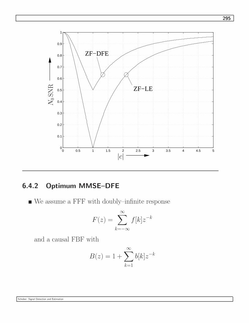
295

0 0.5 1 1.5 2 2.5 3 3.5 4 4.5 50

0.1

0.2

0.3

0.4

0.5

0.6

0.7

0.8

0.9

1

ZF−DFE

ZF−LE

|c|

N0SN

R

6.4.2 Optimum MMSE–DFE

� We assume a FFF with doubly–infinite response

F (z) =

∞∑k=−∞

f [k]z−k

and a causal FBF with

B(z) = 1 +∞∑

k=1

b[k]z−k


296

B(z) − 1

rb[k]F (z)

d[k]I [k]I [k] H(z)

z[k]

y[k]

� Optimization Criterion

In optimum MMSE–DFE, we optimize FFF and FBF for mini-

mization of the variance of the error signal

e[k] = d[k] − I [k].

This error variance can be expressed as

J = E{|e[k]|2

}

= E

{(∞∑

κ=−∞

f [κ]rb[k − κ] −∞∑

κ=1

b[κ]I [k − κ] − I [k]

)

(∞∑

κ=−∞

f∗[κ]r∗b [k − κ] −∞∑

κ=1

b∗[κ]I∗[k − κ] − I∗[k]

)}.

� FFF Optimization

Differentiating J with respect to f∗[ν], −∞ < ν < ∞, yields

∂J

∂f∗[ν]=

∞∑κ=−∞

f [κ] E{rb[k − κ]r∗b [k − ν]}︸︷︷︸φrr[ν−κ]

−

∞∑κ=1

b[κ] E{I [k − κ]r∗b [k − ν]}︸︷︷︸φIr[ν−κ]

−E{I [k]r∗b [k − ν]}︸︷︷︸φIr[ν]


297

Letting ∂J/(∂f∗[ν]) = 0 and taking the Z-transform of the above

equation leads to

F (z)Φrr(z) = B(z)ΦIr(z),

where Φrr(z) and ΦIr(z) denote the Z-transforms of φrr[λ] and

φIr[λ], respectively.

Assuming i.i.d. sequences I [·] of unit variance, we get

Φrr(z) = H(z)H∗(1/z∗) + N0

ΦIr(z) = H∗(1/z∗)

This results in

F (z) =H∗(1/z∗)

H(z)H∗(1/z∗) + N0B(z).

Recall that

FLE(z) =H∗(1/z∗)

H(z)H∗(1/z∗) + N0

is the optimum filter for linear MMSE equalization. This means

the optimum FFF for MMSE–DFE is the cascade of a optimum

linear equalizer and the FBF B(z).

� FBF Optimization

The Z–transform E(z) of the error signal e[k] is given by

E(z) = F (z)Z(z) + (F (z)H(z) − B(z))I(z).

Adopting the optimum F (z), we obtain for the Z–transform of


298

the autocorrelation sequence

Φee(z) = E{E(z)E∗(1/z∗)}

=B(z)B∗(1/z∗)H(z)H∗(1/z∗)

(H(z)H∗(1/z∗) + N0)2N0

+N2

0B(z)B∗(1/z∗)

(H(z)H∗(1/z∗) + N0)2

= B(z)B∗(1/z∗)H(z)H∗(1/z∗) + N0

(H(z)H∗(1/z∗) + N0)2N0

= B(z)B∗(1/z∗)N0

H(z)H∗(1/z∗) + N0︸︷︷︸Φelel

(z)

,

where el[k] denotes the error signal at the output of the optimum

linear MMSE equalizer, and Φelel(z) is the Z–transform of the

autocorrelation sequence of el[k].

The optimum FBF filter will minimize the variance of el[k]. There-

fore, the optimum prediction–error filter for el[k] is the optimum

filter B(z). Consequently, the optimum FBF can be defined as

B(z) =1

Q(z),

where Q(z) is obtained by spectral factorization of Φelel(z)

Φelel(z) =

N0

H(z)H∗(1/z∗) + N0

= σ2eQ(z)Q∗(1/z∗).

The coefficients of q[k], k ≥ 1, can be calculated recursively as

q[k] =

k−1∑µ=0

k − µ

kq[µ]β[k − µ], k ≥ 1


299

with

β[µ] = T

1/(2T )∫

−1/(2T )

ln[Φelel

(ej2πfT )]ej2πµfT df.

The error variance σ2e is given by

σ2e = exp

T

1/(2T )∫

−1/(2T )

ln

[N0

|H(ej2πfT )|2 + N0

]df

.

linearMMSEequalizer

feedback filter

prediction−errorfilter for el[k]

I [k] H(z)

z[k]

F (z)d[k]

I [k]

B(z) − 1

B(z)FLE(z)

� Overall Channel

The overall forward transfer function is given by

Hov(z) = F (z)H(z)

=H(z)H∗(1/z∗)

H(z)H∗(1/z∗) + N0B(z)

=

(1 −

N0

H(z)H∗(1/z∗) + N0

)B(z)

= B(z) −σ2

e

B∗(1/z∗).


300

Therefore, the bias hov[0] is given by

hov[0] = 1 − σ2e .

The part of the transfer function that characterizes the pre–cursors

is given by

−σ2e

(1

B∗(1/z∗)− 1

),

whereas the part of the transfer function that characterizes the

post–cursors is given by

B(z) − 1

Hence, the error signal is composed of bias, pre–cursor ISI, and

noise. The post–cursor ISI is perfectly canceled by the FBF.

� SNR

Taking into account the bias, it can be shown that the SNR for

optimum MMSE DFE is given by

SNRMMSE−DFE =1

σ2e

− 1

= exp

T

1/(2T )∫

−1/(2T )

ln

[|H(ej2πfT )|2

N0+ 1

]df

− 1.

� Remark

For high SNRs, ZF–DFE and MMSE–DFE become equivalent. In

that case, the noise variance is comparatively small and also the

MMSE criterion leads to a complete elimination of the ISI.


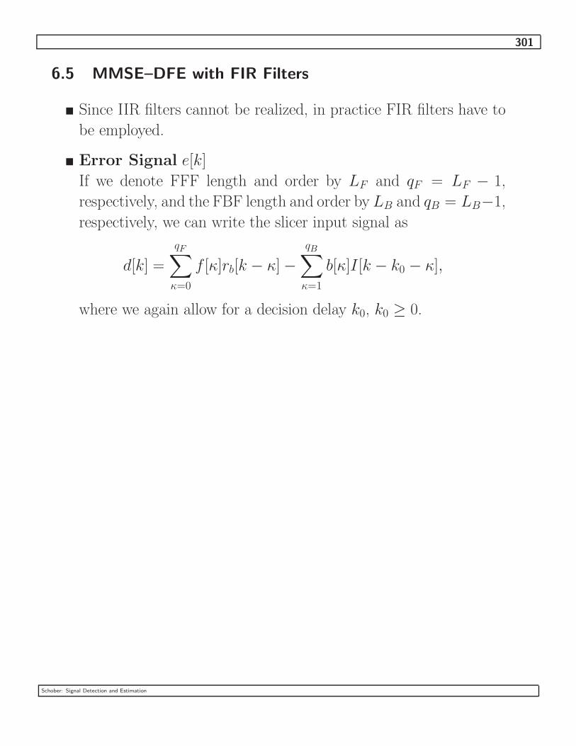
301

6.5 MMSE–DFE with FIR Filters

� Since IIR filters cannot be realized, in practice FIR filters have to

be employed.

� Error Signal e[k]

If we denote FFF length and order by LF and qF = LF − 1,

respectively, and the FBF length and order by LB and qB = LB−1,

respectively, we can write the slicer input signal as

d[k] =

qF∑κ=0

f [κ]rb[k − κ] −

qB∑κ=1

b[κ]I [k − k0 − κ],

where we again allow for a decision delay k0, k0 ≥ 0.


302

Using vector notation, the error signal can be expressed as

e[k] = d[k] − I [k − k0]

= fHrb[k] − bHI [k − k0 − 1] − I [k − k0]

with

f = [f [0] f [1] . . . f [qF ]]H

b = [b[1] f [2] . . . b[qB]]H

rb[k] = [rb[k] rb[k − 1] . . . rb[k − qF ]]T

I [k − k0 − 1] = [I [k − k0 − 1] I [k − k0 − 2] . . . I [k − k0 − qB]]T .

� Error Variance J

The error variance can be obtained as

J = E{|e[k]|2}

= fHE{rb[k]rH

b [k]}f + bHE{I[k − k0 − 1]IH [k − k0 − 1]}b

−fHE{rb[k]IH [k − k0 − 1]}b − bH

E{I[k − k0 − 1]rHb [k]}f

−fHE{rb[k]I∗[k − k0]} − E{rH

b [k]I [k − k0]}f

+bHE{I[k − k0 − 1]I∗[k − k0]} + E{IH [k − k0 − 1]I [k − k0]}b.

Since I [k] is an i.i.d. sequence and the noise z[k] is white, the


303

following identities can be established:

E{I[k − k0 − 1]I∗[k − k0]} = 0

E{I[k − k0 − 1]IH [k − k0 − 1]} = I

E{rb[k]IH [k − k0 − 1]} = H

H =

h[k0 + 1] . . . h[k0 + qB]

h[k0] . . . h[k0 + qB − 1]... . . . ...

h[k0 + 1 − qF ] . . . h[k0 + qB − qF ]

E{rb[k]I∗[k − k0]} = h

h = [h[k0] h[k0 − 1] . . . h[k0 − qF ]]T

E{rb[k]rHb [k]} = Φhh + σ2

nI,

where Φhh denotes the channel autocorrelation matrix. With these

definitions, we get

J = fH(Φhh + σ2nI)f + bHb + 1

−fHHb − bHHHf − fHh − hHf

� Optimum Filters

The optimum filter settings can be obtained by differentiating J

with respect to f ∗ and b∗, respectively.

∂J

∂f ∗ = (Φhh + σ2nI)f − Hb − h

∂J

∂b∗ = b − HHf

Setting the above equations equal to zero and solving for f , we get

f opt =((

Φhh − HHH)

+ σ2nI)−1

h


304

The optimum FBF is given by

bopt = HHf = [hov[k0 + 1] hov[k0 + 1] . . . hov[k0 + qB]]H ,

where hov[k] denotes the overall impulse response comprising chan-

nel and FFF. This means the FBF cancels perfectly the postcursor

ISI.

� MMSE

The MMSE is given by

Jmin = 1 − hH((

Φhh − HHH)

+ σ2nI)−1

h

= 1 − fHopth.

� Bias

The bias is given by

h[k0] = fHopth = 1 − Jmin < 1.


detection and estimation of signals in noise and estimation of signals in noise ... signal detection...

Documents