detection and attribution of temperature changes in...

Detection and Attribution of Temperature Changes in the Mountainous WesternUnited States

CÉLINE BONFILS,* BENJAMIN D. SANTER,* DAVID W. PIERCE,� HUGO G. HIDALGO,� GOVINDASAMY

BALA,* TAPASH DAS,� TIM P. BARNETT,� DANIEL R. CAYAN,�,# CHARLES DOUTRIAUX,*ANDREW W. WOOD,@ ART MIRIN,* AND TORU NOZAWA&

*Lawrence Livermore National Laboratory, Livermore, California�Scripps Institution of Oceanography, La Jolla, California

#U.S. Geological Survey, La Jolla, California@University of Washington, Seattle, Washington

&National Institute for Environmental Studies, Tsukuba, Japan

(Manuscript received 3 January 2008, in final form 22 April 2008)

ABSTRACT

Large changes in the hydrology of the western United States have been observed since the mid-twentiethcentury. These include a reduction in the amount of precipitation arriving as snow, a decline in snowpackat low and midelevations, and a shift toward earlier arrival of both snowmelt and the centroid (center ofmass) of streamflows. To project future water supply reliability, it is crucial to obtain a better understandingof the underlying cause or causes for these changes. A regional warming is often posited as the cause ofthese changes without formal testing of different competitive explanations for the warming. In this study,a rigorous detection and attribution analysis is performed to determine the causes of the late winter/earlyspring changes in hydrologically relevant temperature variables over mountain ranges of the western UnitedStates. Natural internal climate variability, as estimated from two long control climate model simulations,is insufficient to explain the rapid increase in daily minimum and maximum temperatures, the sharp declinein frost days, and the rise in degree-days above 0°C (a simple proxy for temperature-driven snowmelt).These observed changes are also inconsistent with the model-predicted responses to variability in solarirradiance and volcanic activity. The observations are consistent with climate simulations that include thecombined effects of anthropogenic greenhouse gases and aerosols. It is found that, for each temperaturevariable considered, an anthropogenic signal is identifiable in observational fields. The results are robust touncertainties in model-estimated fingerprints and natural variability noise, to the choice of statistical down-scaling method, and to various processing options in the detection and attribution method.

1. Introduction

Winter and spring temperatures over the westernUnited States have warmed significantly during the past50 yr, as witnessed by earlier flower blooms (Cayan etal. 2001). This regional warming has been associatedwith a change of atmospheric circulation over the NorthPacific (Dettinger and Cayan 1995), the origins ofwhich are still under investigation (e.g.: Shindell et al.2001; Gillett et al. 2005; Bonfils et al. 2008). This warm-

ing has been linked to a rise in the number of wildfiresin western U.S. forests (Westerling et al. 2006) and anincrease in the forested area burned over Canada(Gillett and Weaver 2004). Continued warming is likelyto impact crop growth and development (Lobell et al.2006), to exacerbate air pollution and heat waves (Hay-hoe et al. 2004), and to affect the availability of waterresources.

The water resources of the western United Statesdepend on snowpack (e.g., Andreadis and Lettenmaier2006), which stores precipitation during cold monthsand supplies meltwater to river basins during warmmonths. Water managers must balance the competinggoals of meeting water demands while minimizing floodrisk. How climate change will affect this delicate bal-ance is a critical issue for the western United States

Corresponding author address: Céline Bonfils, Program for Cli-mate Model Diagnosis and Intercomparison, Lawrence Liver-more National Laboratory, P.O. Box 808, Mail Stop L-103, Liv-ermore, CA 94550.E-mail: [email protected]

6404 J O U R N A L O F C L I M A T E VOLUME 21

DOI: 10.1175/2008JCLI2397.1

© 2008 American Meteorological Society

JCLI2397

(Maurer et al. 2007). In the past, most decisions onwater supply planning relied on the assumption of astationary climate. This assumption is now being chal-lenged (Gleick et al. 2000; Milly et al. 2008) by theemerging evidence of human-induced changes in theearth’s hydrological cycle (Lambert et al. 2005; Gedneyet al. 2006; Zhang et al. 2007; Santer et al. 2007; Willettet al. 2007) and by various temperature-driven regionalhydrological changes. The snow/rain partitioning ofprecipitation, for instance, has changed with more pre-cipitation falling as rain instead of snow, particularly inregions where mean winter minimum temperature risesabove �5°C and a warming trend bring these tempera-tures near freezing (Knowles et al. 2006). A pervasivedecrease in snow water content and earlier snow melt-ing occur in lower and midelevation mountain areas,particularly at the proximity of the snow line (wherewinter temperature is close to 0°C; Mote et al. 2005).Associated with an increase in January–March tem-peratures, the March fraction of total annual stream-flow rises, while the April–July flows drop, shiftingstreamflow peaks to an earlier date in the year (Det-tinger and Cayan 1995; Stewart et al. 2005).

All these changes may have significant socioeco-nomic impacts on the population of the western UnitedStates, and underscore the urgent need to ensure thatthe best available scientific information on climatechange is well integrated into long-term water manage-ment choices. Informed decision making on water man-agement choices therefore requires a better under-standing of the primary causes of the above-describedobserved changes. While all the cited studies suggestthat these changes may be related to large-scale human-induced warming, this has not yet been demonstrated ina formal detection and attribution (D&A) study.

The current investigation is one of a series of studiesfocusing on the detection and attribution of changes inthe hydrology of the western United States (Barnett etal. 2008; Pierce et al. 2008; Hidalgo et al. 2008, manu-script submitted to J. Climate). We perform a rigorousmodel-based detection and attribution analysis to de-termine the causes of the recent late winter/early springchanges in hydrologically relevant temperature vari-ables. The D&A of changes in snowpack and the timingof streamflow are investigated in Pierce et al. (2008)and Hidalgo et al. (2008, manuscript submitted to J.Climate), respectively. The multivariate D&A analysisthat combines the changes in temperature, snowpack,and timing of the peak streamflow into a single detec-tion variable is discussed in Barnett et al. (2008).

Our study addresses the following questions: Whatare the salient characteristics of the temperature in-crease recently observed over the mountainous regions

of the western United States? Why are temperatureschanging? Are the temperature increases primarilynaturally driven or human induced? Since variations insnow content can arise from temperature changes, pre-cipitation changes, or a combination of the two (e.g.,Groisman et al. 1994; Mote 2006), can we determinewhether earlier snowmelt is primarily caused by tem-perature or precipitation changes?

There are a number of reasons why these questionsare difficult to answer. First, the climate of the westernUnited States is strongly influenced by such natural cli-mate variations as the El Niño–Southern Oscillation(ENSO) and the Pacific decadal oscillation (PDO;Mantua et al. 1997). These modes of variability canstrongly affect the behavior of temperature and hydro-logical variables, and hence complicate the identifica-tion of slow-evolving climate responses to external forc-ings. For example, Mote et al. (2005), Stewart et al.(2005), and Knowles et al. (2006) found that some por-tion of the changes in snowpack, streamflow timing,and snow/rain partitioning could be explained by fluc-tuations in the PDO. ENSO events influence predomi-nantly the interannual variability of western U.S. tem-peratures, extreme precipitation (Cayan et al. 1999),snowfall (Smith and O’Brien 2001), snowpack (Cayan1996), and streamflow (Cayan et al. 1999; Dettinger andCayan 1995).

Second, observed climate changes represent the netresponse of the climate system to multiple forcing fac-tors, plus additional noise from natural internal vari-ability. Use of observational data alone, even in con-junction with sophisticated statistical tools, does notpermit us to unambiguously separate the climatechange contributions from different forcings. Suchseparation can be performed with numerical models,which are frequently used for the systematic experi-mentation that we cannot conduct in the real world.However, all models have errors in both the forcingsthey are run with and the climate responses to thoseforcings. Over the topographically complex westernUnited States, for example, there are small-scale cli-mate features that cannot be resolved with coarse-resolution global climate models. Furthermore, modelexperiments often neglect forcing mechanisms that areknown to be important in the real world, such as thewidespread land-use changes associated with changes inagriculture, urbanization, and irrigation, which canhave a marked influence on the climate of the westernUnited States (Bonfils and Lobell 2007).

There have been a number of attempts to detect hu-man effects on North American climate (Stott 2003;Zwiers and Zhang 2003; Karoly et al. 2003; Karoly andWu 2005). Karoly et al. (2003) found that neither cli-

1 DECEMBER 2008 B O N F I L S E T A L . 6405

mate noise nor natural forcings could explain the largeobserved increase in annual-mean North American sur-face air temperature (30° and 65°N) from 1950 to 1999.Christidis et al. (2007) reported a significant anthropo-genic contribution to North American growing seasonlength, largely because of an earlier date of spring on-set. Finally, Bonfils et al. (2008) showed that the recentwintertime warming over California was inconsistentwith purely natural climate fluctuations and requiredcontributions from one or more external forcings to beexplained. The same study concluded that global cli-mate model simulations fail to reproduce the strongseasonality of Californian temperature trends, probablybecause of their coarse resolution and lack of time-varying land-use forcings.

To our knowledge, no formal D&A study to date hasfocused on the temperature changes occurring overmountainous areas of the western United States, a criti-cal area for the regional hydrology. In the present work,we conduct a formal D&A analysis over nine moun-tainous regions of the west (Fig. 1) using four differenthydrologically related surface air temperature vari-ables. In the detection phase, we investigate whetherthe observed changes in these variables can be fullyexplained by the background “noise” of natural inter-nal climate variability, as estimated from statisticallydownscaled control simulations performed with twodifferent global models. In the attribution phase, weexamine whether the observed changes are consistentwith the twentieth-century climate simulations that in-clude anthropogenic greenhouse gases (GHGs), ozone,and aerosol effects and inconsistent with simulationsthat incorporate solar and volcanic forcing only.

Our D&A analysis relies on climate models that havebeen selected for their ability to capture important fea-tures of the climate of the North Pacific and westernUnited States, such as the mean state and the variabilityassociated with the PDO and ENSO (see sections 2band 3e). Since the effect of finescale orography on tem-perature cannot be adequately represented in coarse-resolution global climate models, we use two differentstatistical “downscaling” techniques to transform datafrom global models to the small spatial scales of interesthere. One underlying assumption in our study is thatthe neglect of changes in irrigation or urbanization inthe model simulations is of less concern in mountainousregions that are of interest here. The detection vari-ables we consider are all directly relevant for under-standing changes in surface hydrology and snowmelt,and include the seasonal averages [January throughMarch (JFM)] of daily minimum and maximum tem-peratures (Tmin, Tmax), the number of frost days (JFMFD), and the number of degree-days above 0°C (JFM

DD � 0). The last variable is a simple proxy for tem-perature-driven snowmelt (see section 2a).

In section 2, we define the temperature indices andintroduce the observational and model data used in ourstudy. A brief description of the two downscaling tech-niques is also provided. In section 3, observed andsimulated temperature trends are compared for each ofthe nine mountain regions. Our D&A technique is de-scribed and applied in section 4. Our focus here is onthe estimated detection times and signal-to-noise (S/N)ratios for an anthropogenic fingerprint together withthe sensitivity of our results to various datasets andprocessing choices. Discussions and conclusions arepresented in section 5.

2. Observational and model data

a. Observational data

Spatial and temporal variations in maximum andminimum temperature for the period 1950–99 were ob-tained from the University of Washington (UW) LandSurface Hydrology Research group in the form of agridded dataset (Hamlet and Lettenmaier 2005). TheUW dataset primarily includes daily-mean data fromthe National Climatic Data Service’s Cooperative Ob-server network (Coop) and monthly-mean data fromthe U.S. Historical Climatology Network (USHCN;Karl et al. 1990). The USHCN data are long recordscorrected for changes in time of observation, stationlocation, instrumentation, and land use. They are usedto include adjustments for temporal inhomogeneities inthe gridded Coop data. The data were interpolated to aregular grid with 1/8° � 1/8° latitude–longitude resolu-tion (about 140 km2 per grid cell).

The JFM Tmin and Tmax are simply computed by av-eraging daily Tmin and Tmax data from 1 January to 31March of each year. The JFM FD index represents thetotal number of days over this period with a daily av-erage temperature below the freezing point. The fourthand final index, DD � 0, measures the extent to whichthe daily average temperature exceeds the meltingpoint (with daily values below 0°C set to zero), andJFM DD � 0 is the sum of each individual day’s DD �0. Quantifying snowmelt from DD � 0 is the simplestapproach used in snowmelt-runoff models when dataon surface energy balances are not available (see, e.g.,Linsley 1943).1 Our use of JFM DD � 0 as a proxy forsnowmelt behavior (instead of the date of the onset ofsnowmelt, which is often difficult to define) is moti-

1 In this technique, the daily snowmelt depth is computed bymultiplying DD � 0 by a melt factor (in mm °C�1 day�1) thatdepends on the physical characteristics of the snow.


vated by the physics of snow: several days with tem-peratures above freezing may be required before anentire snowpack reaches 0°C and begins to melt. Dur-ing the first few days with above-freezing conditions,meltwater produced at the surface of the snowpack maypercolate through the snowpack and refreeze. Refreez-

ing can also occur at night, and it is only after severaldays of sustained above-zero temperatures that thesnowpack structure changes and the melting is efficient.

We focus on mountainous regions of the westernUnited States (which include 10 western states) in thevicinity of snow course stations with a climatological

FIG. 1. Elevation (in meters) and location of the nine mountainous regions over whichtemperature indices are spatially averaged: the Washington Cascades (yellow), the northernRockies (red), the Oregon Cascades (pink), the Blue Mountains (dark blue), the northernSierras (purple), the southern Sierras (brown), the Great Basin (maroon), the Wasatch (lightblue), and the Colorado Rockies (green). Each mountainous region is defined on the 1/8° �1/8° lat–lon grid of the UW observational temperature dataset. Colored circles denote thesnow course locations with a climatological mean snow depth value of at least 1 cm on 1 Apr(Pierce et al. 2008; Barnett et al. 2008). The station network used to create the UW dataset isrepresented by black dots.


Fig 1 live 4/C

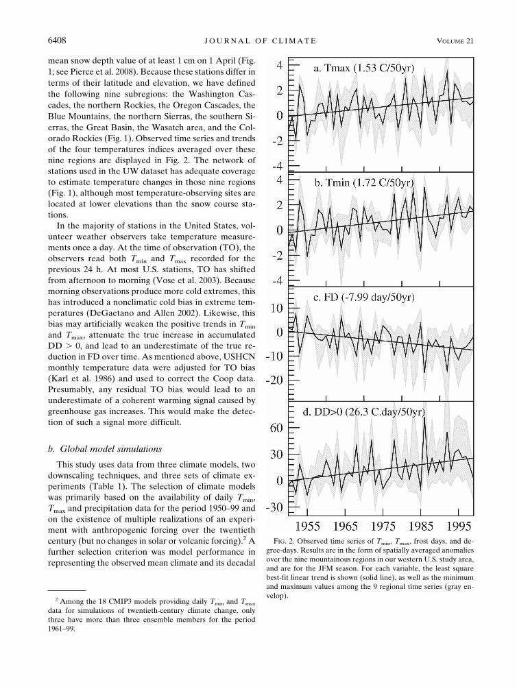
mean snow depth value of at least 1 cm on 1 April (Fig.1; see Pierce et al. 2008). Because these stations differ interms of their latitude and elevation, we have definedthe following nine subregions: the Washington Cas-cades, the northern Rockies, the Oregon Cascades, theBlue Mountains, the northern Sierras, the southern Si-erras, the Great Basin, the Wasatch area, and the Col-orado Rockies (Fig. 1). Observed time series and trendsof the four temperatures indices averaged over thesenine regions are displayed in Fig. 2. The network ofstations used in the UW dataset has adequate coverageto estimate temperature changes in those nine regions(Fig. 1), although most temperature-observing sites arelocated at lower elevations than the snow course sta-tions.

In the majority of stations in the United States, vol-unteer weather observers take temperature measure-ments once a day. At the time of observation (TO), theobservers read both Tmin and Tmax recorded for theprevious 24 h. At most U.S. stations, TO has shiftedfrom afternoon to morning (Vose et al. 2003). Becausemorning observations produce more cold extremes, thishas introduced a nonclimatic cold bias in extreme tem-peratures (DeGaetano and Allen 2002). Likewise, thisbias may artificially weaken the positive trends in Tmin

and Tmax, attenuate the true increase in accumulatedDD � 0, and lead to an underestimate of the true re-duction in FD over time. As mentioned above, USHCNmonthly temperature data were adjusted for TO bias(Karl et al. 1986) and used to correct the Coop data.Presumably, any residual TO bias would lead to anunderestimate of a coherent warming signal caused bygreenhouse gas increases. This would make the detec-tion of such a signal more difficult.

b. Global model simulations

This study uses data from three climate models, twodownscaling techniques, and three sets of climate ex-periments (Table 1). The selection of climate modelswas primarily based on the availability of daily Tmin,Tmax and precipitation data for the period 1950–99 andon the existence of multiple realizations of an experi-ment with anthropogenic forcing over the twentiethcentury (but no changes in solar or volcanic forcing).2 Afurther selection criterion was model performance inrepresenting the observed mean climate and its decadal

2 Among the 18 CMIP3 models providing daily Tmin and Tmax

data for simulations of twentieth-century climate change, onlythree have more than three ensemble members for the period1961–99.

FIG. 2. Observed time series of Tmin, Tmax, frost days, and de-gree-days. Results are in the form of spatially averaged anomaliesover the nine mountainous regions in our western U.S. study area,and are for the JFM season. For each variable, the least squarebest-fit linear trend is shown (solid line), as well as the minimumand maximum values among the 9 regional time series (gray en-velop).


variability over the western United States. Particularattention was focused on the fidelity with which modelsreproduced observed PDO and ENSO characteristicsand on the impacts of these modes of variability onprecipitation patterns.

Natural climate internal variability is estimated fromtwo multicentury preindustrial control simulations per-formed with the finite-volume version of the NationalCenter for Atmospheric Research/Department of En-ergy (NCAR/DOE) Community Climate SystemModel, version 3 (CCSM3-CTL; Bala et al. 2008) andthe DOE/NCAR Parallel Climate Model (PCM-CTL;Washington et al. 2000; Collins et al. 2006). The atmo-spheric components of these models were run at 1.25°longitude � 1° latitude resolution and T42 spectraltruncation, respectively. Both control runs have fixedpreindustrial values of CO2, sulfate aerosols, and tro-pospheric and stratospheric ozone, with no changes insolar irradiance or atmospheric burdens of volcanicaerosols. Our D&A analyses were performed with 850yr of CCSM3-CTL data and 750 yr of PCM-CTL data.The control runs are relatively stationary over the se-lected analysis periods (Bala et al. 2008).

As noted above, the PDO3 and ENSO are importantsources of variability in western U.S. climate. BothCCSM3 and PCM capture key features of the spatialand temporal structure of these natural modes of vari-ability, and are therefore suitable for estimating inter-nal climate noise (see Fig. 2 of Pierce et al. 2008; Al-exander et al. 2006; Meehl and Hu 2006). The leadingmode of ENSO variability has spatial structure similarto that of observations, although it extends too far intothe west Pacific (Pierce et al. 2008). The spatial pattern

of the PDO in the CCSM3-CTL and PCM-CTL cap-tures the observed “horseshoe” shape over the NorthPacific Ocean. The peak loading is correctly positionedover the central Pacific in the PCM-CTL but is dis-placed toward Japan in CCSM3-CTL (Pierce et al.2008).

These features of the PDO are also apparent in allCoupled Model Intercomparison Project phase 3(CMIP3) twentieth-century runs performed with PCMand the T85 version of CCSM3. Spatial correlationsbetween the observed PDO pattern and the patternssimulated in the CCSM3 and PCM twentieth-centuryruns typically range from 0.86 to 0.91, respectively. Ondecadal time scales, the amplitude of SST variability inthe PDO region is roughly 25%–30% higher than ob-served in PCM and 15% lower than observed inCCSM3. There is no evidence, therefore, that the twocontrol simulations significantly underestimate eitherENSO or PDO variability (see further discussion insection 3e). PCM also captures features of the observedsecular changes in sea surface temperatures, such as theprominent “regime change” in the mid-1970s. In themodel, this shift is primarily due to a combination ofinternally generated variability and anthropogenic forc-ing (Meehl et al. 2009). Finally, we note that both PCMand CCSM3 successfully replicate the pattern of clima-tological mean December–February (DJF) precipita-tion over the western United States, as estimated fromthe National Centers for Environmental Prediction(NCEP) Global Reanalysis (Kalnay et al. 1996) overthe 1949–98 period (r � 0.9).

The anthropogenic signal was estimated from twoensembles of historical simulations: a 4-member en-semble4 performed with PCM (PCM-ANTH) and a 10-member ensemble generated with the T42-resolution

3 The PDO is defined here as the leading EOF of wintertimenorthern Pacific sea surface temperatures. The regional mean seasurface temperatures is subtracted prior to calculation of EOFs. 4 The runs analyzed were B06.22, B06.23, B06.27, and B06.28.

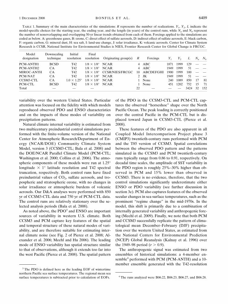
TABLE 1. Summary of the main characteristics of the simulations: R represents the number of realizations. Y1, Y2, L indicate themodel-specific choices for the starting year, the ending year, and the length (in years) of the control runs, while Na and Nb representthe number of nonoverlapping and overlapping 50-yr linear trends obtained from each of them. Forcings applied to the simulations arecoded as below. A: greenhouse gases, B: ozone, C: direct effect of sulfate aerosols, D: indirect effect of sulfate aerosols, E: black carbon,F: organic carbon, G: mineral dust, H: sea salt, I: land-use change, J: solar irradiance, K: volcanic aerosols. Center for Climate SystemResearch is CCSR, National Institute for Environmental Studies is NIES, Frontier Research Center for Global Change is FRCGC.

Modeldesignation

Downscalingtechnique

Initialresolution

Finalresolution Originating group(s) R Forcings Y1 Y2 L Na Nb

PCM-ANTH1 BCSD T42 1/8 � 1/8° NCAR 4 ABC 1871 1999 129 — —PCM-ANTH2 CA T42 1/8 � 1/8° NCAR 4 ABC 1949 1999 51 — —MIROC-ANTH CA T42 1/8 � 1/8° CCSR/NIES/FRCGC 10 ABCDEFGHI 1900 1999 100 — —PCM-NAT CA T42 1/8 � 1/8° NCAR 2 JK 1949 1999 51 — —CCSM3-CTL CA 1.0 � 1.25° 1/8 � 1/8° NCAR 1 None 240 1089 850 17 81PCM-CTL BCSD T42 1/8 � 1/8° NCAR 1 None 451 1202 752 15 71Total — — — 22 — — — 3424 32 152


(“Medres”) version of the Model for InterdisciplinaryResearch on Climate 3.2 (MIROC3.2) model (MIROC-ANTH). PCM-ANTH runs include changes in well-mixed greenhouse gases, tropospheric and strato-spheric ozone, and the direct scattering effects of sul-fate aerosols. MIROC-ANTH (K-1 model developers2004; Nozawa et al. 2007) additionally includes the di-rect effects of carbonaceous aerosols, and some indirecteffects of both sulfate and carbonaceous aerosols onclouds (see Santer et al. 2007 and Table 1 for a com-plete list of forcings). All CMIP3 twentieth-centuryruns performed with the MIROC T42 model replicatethe observed structure of the PDO, although peak load-ings of the leading EOF are misplaced and slightly un-derestimated (not shown). The spatial correlation withobservations (r � 0.72) is slightly lower than forCCSM3 or PCM, but the MIROC T42 models stillranks among the top CMIP3 models in terms of itsrepresentation of the spatial structure of the PDO. TheMIROC model depicts a PDO frequency spectrumcomparable to observations (Shiogama et al. 2005).

Finally, to characterize the climate response to natu-ral external forcings, we analyze two PCM simulationswhich are forced solely by historical changes in solarirradiance and volcanic aerosols (PCM-NAT; casesB06.68 and B06.69).

c. Downscaling techniques

The western United States is climatologically com-plex; its topography is not well represented by thecoarse resolution of most climate models: even the bestmodels display climate biases at regional scales (Mau-rer and Hidalgo 2007). To better capture the nuances ofthe climate changes over mountainous regions and atthe spatial scales of large river basins as required by ourstudy, the daily precipitation, Tmin, and Tmax data fromall climate simulations were first statistically down-scaled, and then used to force the variable infiltrationcapacity (VIC) hydrological model (Liang et al. 1994;Cherkauer and Lettenmaier 2003). Two downscalingapproaches were employed here: the constructed ana-logs technique (CA; H. G. Hidalgo et al. 2008) and thebias-correction and spatial downscaling procedure(BCSD; Wood et al. 2004). The use of two differentmethods provides useful information on the sensitivityof D&A results to the choice of statistical downscalingtechnique.

The CA technique estimates a daily “target pattern”of Tmin, Tmax, or precipitation from a climate model.This target is a linear combination of observed dailypatterns that have been aggregated to the climatemodel resolution (the analog). The downscaled dataare generated by applying the estimated regression co-

efficients for the “target pattern” to the corresponding1/8°-resolution daily observed patterns.

The BCSD method generates climatological cumula-tive distribution functions of the monthly-mean climatemodel data (over the period 1950–99) and maps theirquantiles onto those of gridded observations aggre-gated to the climate model resolution. Anomalies of thebias-corrected model variables are then formed relativeto the climatological reference period, interpolated to1/8° resolution, and added to the 1/8° gridded observa-tional means. The final step of this procedure is to gen-erate daily forcing fields by a resampling and rescalingtechnique. The BCSD method yields bias-correcteddaily temperature and precipitation outputs that pre-serve the mean, variability, and temporal evolution ofthe monthly-mean data (Maurer et al. 2007). Details ofthe techniques are given in H. G. Hidalgo et al. (2008)and Wood et al. (2004), and their performance is com-pared in Maurer and Hidalgo (2007).

To investigate whether the anthropogenic signal issensitive to the choice of downscaling technique, thefour PCM anthropogenic runs were downscaled usingboth the BCSD approach (PCM-ANTH1) as well as theCA method (PCM-ANTH2). All other simulationswere downscaled with one of the two techniques only:BCSD was used for the PCM-CTL run, while the CAmethod was applied for the CCSM3-CTL run, theMIROC anthropogenic runs, and PCM-NAT experi-ment (see Table 1). The four temperature variables em-ployed in the D&A analysis were calculated from thestatistically downscaled Tmin and Tmax data and (in thecase of the FD and DD � 0 indices) from the surface airtemperature recalculated by the VIC model after esti-mating a diurnal cycle of temperature from Tmin andTmax.

d. Correlation of temperature indices with SWE/P

Each of the selected temperature indices is expectedto show some relationship with changes in aspects ofthe hydrological cycle. For each of the nine regions, wecomputed the correlation between 1 April snow waterequivalent (SWE) divided by the accumulated Octo-ber–March precipitation (SWE/P; see Pierce et al.2008) and the four different JFM temperature indicesover the period 1950–99 (Fig. 3). SWE is divided byP to reduce the influence of precipitation fluctuationson the variability and trends in SWE, and hence high-light trends in the temperature-driven component ofSWE.

In both observations (Fig. 3a) and the PCM-ANTH1results (Fig. 3b), SWE/P changes over 1950–99 are in-versely correlated with temperature changes. In PCM-ANTH1 and the observations, the DD � 0, FD, and


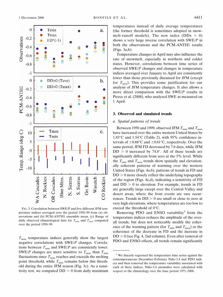
Tmax temperature indices generally show the largestnegative correlations with SWE/P changes. Correla-tions between Tmin and SWE/P are consistently lower.SWE/P changes are more sensitive to Tmax than Tmin

fluctuations since Tmax reaches and exceeds the meltingpoint threshold, while Tmin remains below this thresh-old during the entire JFM season (Fig. 3c). As a sensi-tivity test, we computed DD � 0 from daily maximum

temperatures instead of daily average temperatures(the former threshold is sometimes adopted in snow-melt-runoff models). The new index (DDx � 0)shows a very large inverse correlation with SWE/P inboth the observations and the PCM-ANTH1 results(Figs. 3a,b).

Temperature changes in April may also influence therate of snowmelt, especially in northern and colderstates. However, correlations between time series ofobserved SWE/P changes and changes in temperatureindices averaged over January to April are consistentlylower than those previously discussed for JFM (exceptfor Tmin). This provides some justification for ouranalysis of JFM temperature changes. It also allows amore direct comparison with the SWE/P results inPierce et al. (2008), who analyzed SWE as measured on1 April.

3. Observed and simulated trends

a. Spatial patterns of trends

Between 1950 and 1999, observed JFM Tmin and Tmax

have increased over the entire western United States by1.83°C and 1.54°C (Table 2), with 95% confidence in-tervals of �0.68°C and �0.61°C, respectively. Over thesame period, JFM FD decreased by 7.6 days, while JFMDD � 0 increased by 74.8°. All of these trends aresignificantly different from zero at the 5% level. Whilethe Tmin and Tmax trends show spatially and elevation-ally coherent patterns of warming over the westernUnited States (Figs. 4a,b), patterns of trends in FD andDD � 0 more closely reflect the underlying topographyof the region (Figs. 4c,d), indicating a sensitivity of FDand DD � 0 to elevation. For example, trends in FDare generally large except over the Central Valley anddesert areas, where the frost events are rare occur-rences. Trends in DD � 0 are small or close to zero atvery high elevations, where temperatures are too low toexceed the threshold of 0°C.

Removing PDO and ENSO variability5 from thetemperature indices reduces the amplitude of the over-all trends, but does not noticeably modify the coher-ence of the warming pattern (for Tmin and Tmax) or thecoherence of the decrease in FD and the increase inDD � 0 (see Fig. 4, 2nd column). Even after removal ofPDO and ENSO effects, all trends remain significantly

5 We linearly regressed the temperature time series against thecontemporaneous December–February Niño-3.4 and PDO indi-ces and then removed the temperature variability associated witheach of these indices. Niño-3.4 anomalies were calculated withrespect to the climatology over the base period 1971–2000.

FIG. 3. Correlation between SWE/P and five different JFM tem-perature indices averaged over the period 1950–99 from (a) ob-servations and (b) PCM-ANTH1 ensemble mean. (c) Range ofdaily observed climatological data for Tmin and Tmax computedover the period 1950–99.


Fig 3 live 4/C

different from zero at the 5% level. For comparison,spatial trends for one of the four downscaled PCM-ANTH1 realization (B06.28) are also presented (Fig. 4,3rd column). The general structure and amplitude ofthe simulated trends is consistent with observations.The most noticeable difference is that the simulatedpatterns of Tmin and Tmax changes show less spatialheterogeneity than the corresponding observed results.The observed sensitivity of the amplitude of FD andDD � 0 trends amplitudes to elevation is well capturedby the model. Regression-based removal of PDO andENSO signals from these temperature indices has alarger impact in the selected PCM simulation than inobservations (Fig. 4; compare 2nd and 4th columns).

b. Comparison of observed and unforced trends inmountainous regions

Observed trends over 1950–99 in the nine mountainregions were computed for all four temperature indi-ces6 (Fig. 2). A standard statistical test of trend signifi-cance (Santer et al. 2000a) reveals that in all cases ex-cept one (the Tmax trend in the Colorado Rockies) ob-served trends are significantly different from zero at the5% level.7 A related question is whether natural inter-nal climate variability, as simulated by the CCSM3 andPCM models, could explain the observed 50-yr trends.To address this question, we calculated (separately foreach index and each region) 50-yr trends from theCCSM3-CTL and PCM-CTL runs. This was done forboth nonoverlapping trends and for trends that over-lapped by all but 10 yr. We then pooled results fromboth control runs to form 36 sampling distributions ofunforced trends (9 regions � 4 indices). For the case ofoverlapping 50-yr trends, this procedure yields a totalof 152 samples (see Table 1), from which we can esti-mate the probability (i.e., the p value) that the observedtrend could be due to climate noise alone. Note that the

use of overlapping trends yields smoother estimates ofthe underlying sampling distributions but has relativelylittle influence on the estimated p values.

Assuming that the model-based estimates of internalclimate noise are reliable (see sections 2b and 3e), weconclude that, in 27 (31) out of 36 cases, observedtrends are significantly different from internal climatevariability at the 5% level using a two-tailed test (usinga one-tailed test).8 Intriguingly, the southern Sierrasyields nonsignificant trends for three of the four tem-perature indices. This is the only region that experi-ences a slight (although nonsignificant) increase insnowpack (Pierce et al. 2008). In summary, our simpletrend comparison analysis suggests that, for most vari-ables and in most regions, internal climate variabilityalone cannot explain the observed long-term tempera-ture changes over the last 50 yr.

c. Comparison of unforced and anthropogenicallyforced trends

We consider next whether the observed changes areconsistent with model results from anthropogenicallyforced simulations. Before addressing this question, wewould like to assess (for each region and temperatureindex) whether the distribution of ANTHRO trendsdiffers significantly from the pooled distribution of un-forced trends obtained from the CCSM3-CTL andPCM-CTL runs.

As expected, trends from individual ANTH realiza-tions show considerable between-realization variability(see Fig. 5). For example, while trends from three PCMANTH realizations (B06.22, B06.27, and B06.28) havethe same sign as the observed trends for all four tem-perature indices, one realization (B06.23) has changesof opposite sign. Trends obtained with CA downscalingare weaker than those obtained with BCSD, in agree-ment with the results of Maurer and Hidalgo (2007). Ofthe 10 MIROC-ANTH simulations, 5 yield changesthat are consistent in sign with the observations. The

6 Observed time series for Tmin in the Washington Cascades,northern Rockies, and northern Sierras are shown in Barnett et al.(2008).

7 This test of trend significance accounts for temporal autocor-relation of the regression residuals in estimating both the standarderror of the trend and the degrees of freedom for the t test oftrend significance.

8 This is a reasonable assumption since we a priori expect awarming in North America (Karoly et al. 2003) and in California(Bonfils et al. 2008), with a subsequent reduction in FD and in-crease in DD � 0.

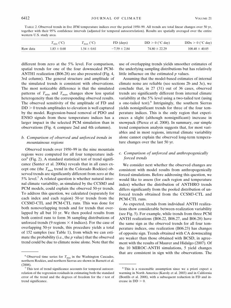
TABLE 2. Observed trends in five JFM temperature indices over the period 1950–99. All trends are total linear changes over 50 yr,together with their 95% confidence intervals (adjusted for temporal autocorrelation). Results are spatially averaged over the entirewestern U.S. study area.

Tmin (°C) Tmax (°C) FD (days) DD � 0 (°C day) DDx � 0 (°C day)

Raw data 1.83 � 0.68 1.54 � 0.61 �7.59 � 2.84 74.80 � 22.29 108.48 � 40.05


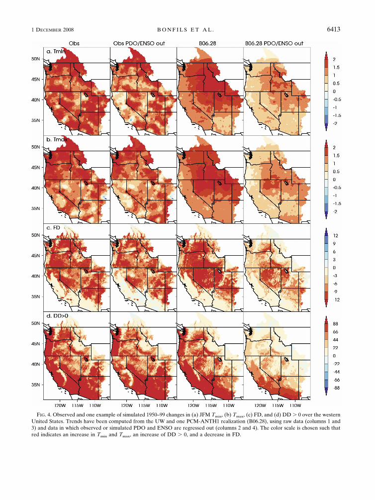
FIG. 4. Observed and one example of simulated 1950–99 changes in (a) JFM Tmin, (b) Tmax, (c) FD, and (d) DD � 0 over the westernUnited States. Trends have been computed from the UW and one PCM-ANTH1 realization (B06.28), using raw data (columns 1 and3) and data in which observed or simulated PDO and ENSO are regressed out (columns 2 and 4). The color scale is chosen such thatred indicates an increase in Tmin and Tmax, an increase of DD � 0, and a decrease in FD.


Fig 4 live 4/C

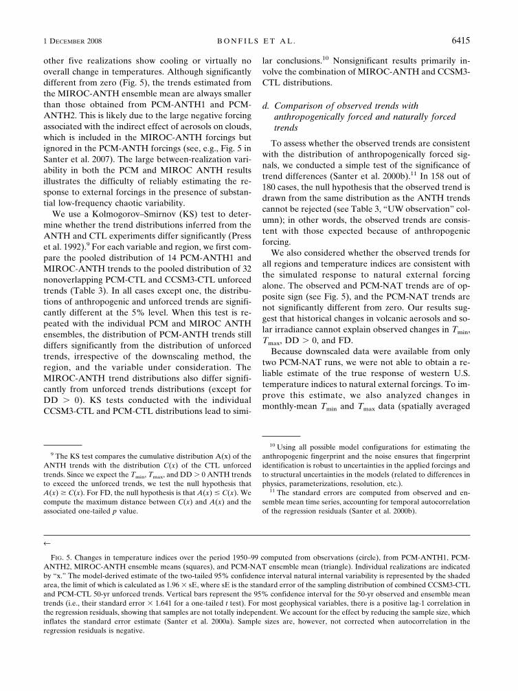
other five realizations show cooling or virtually nooverall change in temperatures. Although significantlydifferent from zero (Fig. 5), the trends estimated fromthe MIROC-ANTH ensemble mean are always smallerthan those obtained from PCM-ANTH1 and PCM-ANTH2. This is likely due to the large negative forcingassociated with the indirect effect of aerosols on clouds,which is included in the MIROC-ANTH forcings butignored in the PCM-ANTH forcings (see, e.g., Fig. 5 inSanter et al. 2007). The large between-realization vari-ability in both the PCM and MIROC ANTH resultsillustrates the difficulty of reliably estimating the re-sponse to external forcings in the presence of substan-tial low-frequency chaotic variability.

We use a Kolmogorov–Smirnov (KS) test to deter-mine whether the trend distributions inferred from theANTH and CTL experiments differ significantly (Presset al. 1992).9 For each variable and region, we first com-pare the pooled distribution of 14 PCM-ANTH1 andMIROC-ANTH trends to the pooled distribution of 32nonoverlapping PCM-CTL and CCSM3-CTL unforcedtrends (Table 3). In all cases except one, the distribu-tions of anthropogenic and unforced trends are signifi-cantly different at the 5% level. When this test is re-peated with the individual PCM and MIROC ANTHensembles, the distribution of PCM-ANTH trends stilldiffers significantly from the distribution of unforcedtrends, irrespective of the downscaling method, theregion, and the variable under consideration. TheMIROC-ANTH trend distributions also differ signifi-cantly from unforced trends distributions (except forDD � 0). KS tests conducted with the individualCCSM3-CTL and PCM-CTL distributions lead to simi-

lar conclusions.10 Nonsignificant results primarily in-volve the combination of MIROC-ANTH and CCSM3-CTL distributions.

d. Comparison of observed trends withanthropogenically forced and naturally forcedtrends

To assess whether the observed trends are consistentwith the distribution of anthropogenically forced sig-nals, we conducted a simple test of the significance oftrend differences (Santer et al. 2000b).11 In 158 out of180 cases, the null hypothesis that the observed trend isdrawn from the same distribution as the ANTH trendscannot be rejected (see Table 3, “UW observation” col-umn); in other words, the observed trends are consis-tent with those expected because of anthropogenicforcing.

We also considered whether the observed trends forall regions and temperature indices are consistent withthe simulated response to natural external forcingalone. The observed and PCM-NAT trends are of op-posite sign (see Fig. 5), and the PCM-NAT trends arenot significantly different from zero. Our results sug-gest that historical changes in volcanic aerosols and so-lar irradiance cannot explain observed changes in Tmin,Tmax, DD � 0, and FD.

Because downscaled data were available from onlytwo PCM-NAT runs, we were not able to obtain a re-liable estimate of the true response of western U.S.temperature indices to natural external forcings. To im-prove this estimate, we also analyzed changes inmonthly-mean Tmin and Tmax data (spatially averaged

9 The KS test compares the cumulative distribution A(x) of theANTH trends with the distribution C(x) of the CTL unforcedtrends. Since we expect the Tmin, Tmax, and DD � 0 ANTH trendsto exceed the unforced trends, we test the null hypothesis thatA(x) � C(x). For FD, the null hypothesis is that A(x) � C(x). Wecompute the maximum distance between C(x) and A(x) and theassociated one-tailed p value.

10 Using all possible model configurations for estimating theanthropogenic fingerprint and the noise ensures that fingerprintidentification is robust to uncertainties in the applied forcings andto structural uncertainties in the models (related to differences inphysics, parameterizations, resolution, etc.).

11 The standard errors are computed from observed and en-semble mean time series, accounting for temporal autocorrelationof the regression residuals (Santer et al. 2000b).

←

FIG. 5. Changes in temperature indices over the period 1950–99 computed from observations (circle), from PCM-ANTH1, PCM-ANTH2, MIROC-ANTH ensemble means (squares), and PCM-NAT ensemble mean (triangle). Individual realizations are indicatedby “x.” The model-derived estimate of the two-tailed 95% confidence interval natural internal variability is represented by the shadedarea, the limit of which is calculated as 1.96 � sE, where sE is the standard error of the sampling distribution of combined CCSM3-CTLand PCM-CTL 50-yr unforced trends. Vertical bars represent the 95% confidence interval for the 50-yr observed and ensemble meantrends (i.e., their standard error � 1.641 for a one-tailed t test). For most geophysical variables, there is a positive lag-1 correlation inthe regression residuals, showing that samples are not totally independent. We account for the effect by reducing the sample size, whichinflates the standard error estimate (Santer et al. 2000a). Sample sizes are, however, not corrected when autocorrelation in theregression residuals is negative.


TA

BL

E3.

Res

ults

ofK

Ste

stto

dete

rmin

ew

heth

erth

ean

thro

poge

nic

sign

alst

reng

ths

are

stat

isti

cally

diff

eren

tfr

omth

epo

pula

tion

ofun

forc

edtr

ends

.T

ests

are

cond

ucte

dus

ing

indi

vidu

alor

com

bine

dru

ns(t

he“c

ombi

ned”

case

inth

ese

cond

colu

mn

com

bine

sP

CM

-AN

TH

1an

dM

IRO

C-A

NT

Hen

sem

ble

mea

ns).

Acr

oss

indi

cate

sth

ean

thro

poge

nic

and

unfo

rced

tren

dsar

est

atis

tica

llydi

ffer

ent

atth

e5%

sign

ific

ance

leve

l.A

circ

lein

dica

tes

the

obse

rved

tren

dis

cons

iste

ntw

ith

the

dist

ribu

tion

oftr

ends

obta

ined

wit

han

thro

poge

nic

forc

ing

(i.e

.,th

enu

llhy

poth

esis

that

the

obse

rved

tren

dca

nbe

draw

nfr

omth

esa

me

dist

ribu

tion

asth

eA

NT

Htr

ends

isno

tre

ject

edat

the

5%si

gnif

ican

cele

vel,

usin

ga

test

ofsi

gnif

ican

ceof

the

diff

eren

cebe

twee

ntw

opo

pula

tion

s’m

eans

;see

text

for

deta

ils).

Com

bine

dC

TL

FV

-CT

LP

CM

-CT

LU

WO

BSE

RV

AT

ION

BM

CR

GB

NR

NS

OR

SSW

AW

HB

MC

RG

BN

RN

SO

RSS

WA

WH

BM

CR

GB

NR

NS

OR

SSW

AW

HB

MC

RG

BN

RN

SO

RSS

WA

WH

Tm

inC

ombi

ned

��

��

��

��

��

��

��

��

��

��

��

��

��

��

��

��

��

�P

CM

-AN

TH

1�

��

��

��

��

��

��

��

��

��

��

��

��

��

��

��

��

��

PC

M-A

NT

H2

��

��

��

��

��

��

��

��

��

��

��

��

��

��

��

��

��

��

MIR

OC

-AN

TH

��

��

��

��

��

��

��

��

��

��

��

��

��

��

��

�T

max

Com

bine

d�

��

��

��

��

��

��

��

��

��

��

��

��

��

��

��

��

�P

CM

-AN

TH

1�

��

��

��

��

��

��

��

��

��

��

��

��

��

��

��

��

��

PC

M-A

NT

H2

��

��

��

��

��

��

��

��

��

��

��

��

��

��

��

��

��

��

MIR

OC

-AN

TH

��

��

��

��

��

��

��

��

��

��

��

��

�F

DC

ombi

ned

��

��

��

��

��

��

��

��

��

��

��

��

��

��

��

��

��

��

PC

M-A

NT

H1

��

��

��

��

��

��

��

��

��

��

��

��

��

��

��

��

��

�P

CM

-AN

TH

2�

��

��

��

��

��

��

��

��

��

��

��

��

��

��

��

��

��

�M

IRO

C-A

NT

H�

��

��

��

��

��

��

��

��

��

��

��

��

��

��

�D

D�

0C

ombi

ned

��

��

��

��

��

��

��

��

��

��

��

��

��

��

��

�P

CM

-AN

TH

1�

��

��

��

��

��

��

��

��

��

��

��

��

��

��

��

��

��

PC

M-A

NT

H2

��

��

��

��

��

��

��

��

��

��

��

��

��

��

��

��

��

MIR

OC

-AN

TH

��

��

��

��

��

��

��

��

��

��

DD

x�

0C

ombi

ned

��

��

��

��

��

��

��

��

��

��

��

��

��

��

��

��

PC

M-A

NT

H1

��

��

��

��

��

��

��

��

��

��

��

��

��

��

��

��

��

�P

CM

-AN

TH

2�

��

��

��

��

��

��

��

��

��

��

��

��

��

��

��

��

��

MIR

OC

-AN

TH

��

��

��

��

��

��

��

��

��

��

��

��

��


over the entire western United States) in 4 PCM-NATruns and in 32 additional PCM-based estimates of “to-tal” natural variability.

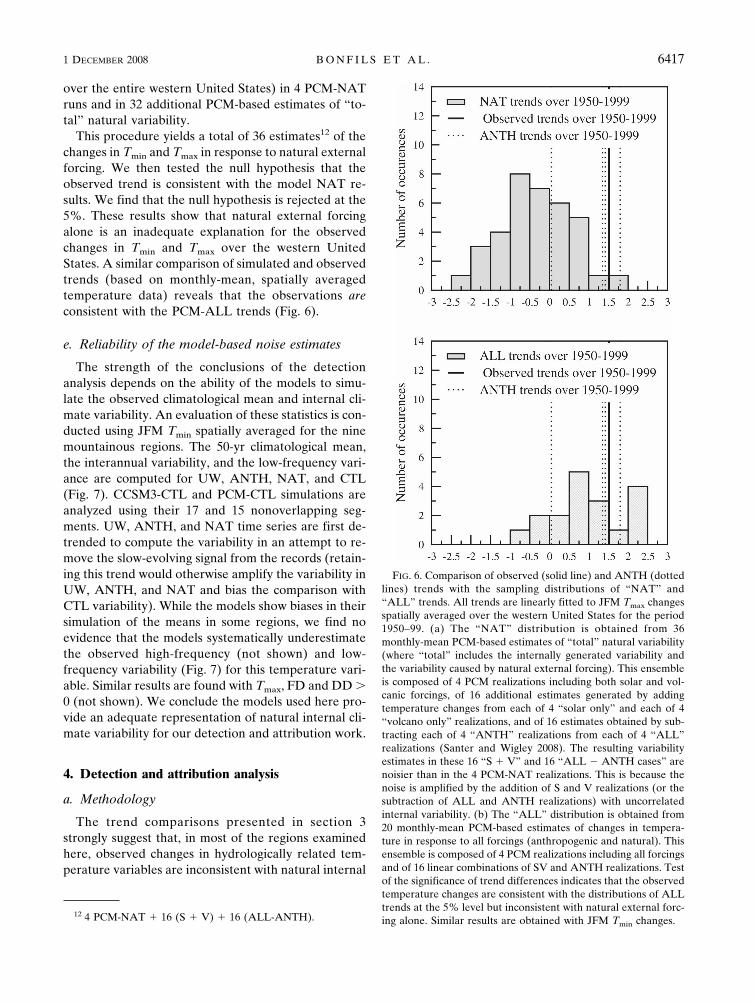
This procedure yields a total of 36 estimates12 of thechanges in Tmin and Tmax in response to natural externalforcing. We then tested the null hypothesis that theobserved trend is consistent with the model NAT re-sults. We find that the null hypothesis is rejected at the5%. These results show that natural external forcingalone is an inadequate explanation for the observedchanges in Tmin and Tmax over the western UnitedStates. A similar comparison of simulated and observedtrends (based on monthly-mean, spatially averagedtemperature data) reveals that the observations areconsistent with the PCM-ALL trends (Fig. 6).

e. Reliability of the model-based noise estimates

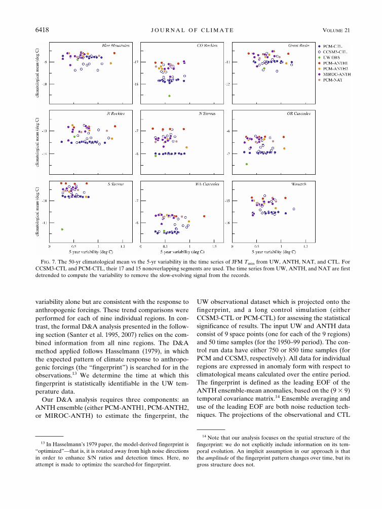
The strength of the conclusions of the detectionanalysis depends on the ability of the models to simu-late the observed climatological mean and internal cli-mate variability. An evaluation of these statistics is con-ducted using JFM Tmin spatially averaged for the ninemountainous regions. The 50-yr climatological mean,the interannual variability, and the low-frequency vari-ance are computed for UW, ANTH, NAT, and CTL(Fig. 7). CCSM3-CTL and PCM-CTL simulations areanalyzed using their 17 and 15 nonoverlapping seg-ments. UW, ANTH, and NAT time series are first de-trended to compute the variability in an attempt to re-move the slow-evolving signal from the records (retain-ing this trend would otherwise amplify the variability inUW, ANTH, and NAT and bias the comparison withCTL variability). While the models show biases in theirsimulation of the means in some regions, we find noevidence that the models systematically underestimatethe observed high-frequency (not shown) and low-frequency variability (Fig. 7) for this temperature vari-able. Similar results are found with Tmax, FD and DD �0 (not shown). We conclude the models used here pro-vide an adequate representation of natural internal cli-mate variability for our detection and attribution work.

4. Detection and attribution analysis

a. Methodology

The trend comparisons presented in section 3strongly suggest that, in most of the regions examinedhere, observed changes in hydrologically related tem-perature variables are inconsistent with natural internal

12 4 PCM-NAT � 16 (S � V) � 16 (ALL-ANTH).

FIG. 6. Comparison of observed (solid line) and ANTH (dottedlines) trends with the sampling distributions of “NAT” and“ALL” trends. All trends are linearly fitted to JFM Tmax changesspatially averaged over the western United States for the period1950–99. (a) The “NAT” distribution is obtained from 36monthly-mean PCM-based estimates of “total” natural variability(where “total” includes the internally generated variability andthe variability caused by natural external forcing). This ensembleis composed of 4 PCM realizations including both solar and vol-canic forcings, of 16 additional estimates generated by addingtemperature changes from each of 4 “solar only” and each of 4“volcano only” realizations, and of 16 estimates obtained by sub-tracting each of 4 “ANTH” realizations from each of 4 “ALL”realizations (Santer and Wigley 2008). The resulting variabilityestimates in these 16 “S � V” and 16 “ALL � ANTH cases” arenoisier than in the 4 PCM-NAT realizations. This is because thenoise is amplified by the addition of S and V realizations (or thesubtraction of ALL and ANTH realizations) with uncorrelatedinternal variability. (b) The “ALL” distribution is obtained from20 monthly-mean PCM-based estimates of changes in tempera-ture in response to all forcings (anthropogenic and natural). Thisensemble is composed of 4 PCM realizations including all forcingsand of 16 linear combinations of SV and ANTH realizations. Testof the significance of trend differences indicates that the observedtemperature changes are consistent with the distributions of ALLtrends at the 5% level but inconsistent with natural external forc-ing alone. Similar results are obtained with JFM Tmin changes.


variability alone but are consistent with the response toanthropogenic forcings. These trend comparisons wereperformed for each of nine individual regions. In con-trast, the formal D&A analysis presented in the follow-ing section (Santer et al. 1995, 2007) relies on the com-bined information from all nine regions. The D&Amethod applied follows Hasselmann (1979), in whichthe expected pattern of climate response to anthropo-genic forcings (the “fingerprint”) is searched for in theobservations.13 We determine the time at which thisfingerprint is statistically identifiable in the UW tem-perature data.

Our D&A analysis requires three components: anANTH ensemble (either PCM-ANTH1, PCM-ANTH2,or MIROC-ANTH) to estimate the fingerprint, the

UW observational dataset which is projected onto thefingerprint, and a long control simulation (eitherCCSM3-CTL or PCM-CTL) for assessing the statisticalsignificance of results. The input UW and ANTH dataconsist of 9 space points (one for each of the 9 regions)and 50 time samples (for the 1950–99 period). The con-trol run data have either 750 or 850 time samples (forPCM and CCSM3, respectively). All data for individualregions are expressed in anomaly form with respect toclimatological means calculated over the entire period.The fingerprint is defined as the leading EOF of theANTH ensemble-mean anomalies, based on the (9 � 9)temporal covariance matrix.14 Ensemble averaging anduse of the leading EOF are both noise reduction tech-niques. The projections of the observational and CTL

13 In Hasselmann’s 1979 paper, the model-derived fingerprint is“optimized”—that is, it is rotated away from high noise directionsin order to enhance S/N ratios and detection times. Here, noattempt is made to optimize the searched-for fingerprint.

14 Note that our analysis focuses on the spatial structure of thefingerprint: we do not explicitly include information on its tem-poral evolution. An implicit assumption in our approach is thatthe amplitude of the fingerprint pattern changes over time, but itsgross structure does not.

FIG. 7. The 50-yr climatological mean vs the 5-yr variability in the time series of JFM Tmin from UW, ANTH, NAT, and CTL. ForCCSM3-CTL and PCM-CTL, their 17 and 15 nonoverlapping segments are used. The time series from UW, ANTH, and NAT are firstdetrended to compute the variability to remove the slow-evolving signal from the records.


Fig 7 live 4/C

anomaly data onto the fingerprint yield the signal andnoise time series Z(t) and N(t), respectively.

b. Example of detection of changes in JFM Tmin

In the following, we analyze the JFM Tmin case, usingthe mean of the PCM-ANTH1 ensemble to estimatethe anthropogenic fingerprint, the CCSM3-CTL to as-sess the statistical significance, and the UW observa-tions. In the baseline “no weighting” case, we assigneach region unit weight despite differences in their spa-tial coverage.

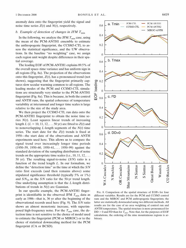
The leading EOF of PCM-ANTH1 explains 89.5% ofthe overall space–time variance and has uniform sign inall regions (Fig. 8a). The projection of the observationsonto this fingerprint, Z(t), has a pronounced trend (notshown), suggesting that the fingerprint primarily cap-tures slow secular warming common to all regions. Theleading modes of the PCM and CCSM3-CTL simula-tions are structurally very similar to the PCM-ANTH1fingerprint (Fig. 8a). This is because, in both the controland ANTH runs, the spatial coherence of temperaturevariability at interannual and longer time scales is largerelative to the size of the study area.

We then project the CCSM3-CTL run data onto thePCM-ANTH1 fingerprint to obtain the noise time se-ries N(t). Least squares linear trends of increasinglength L (L � 10, 11, 12, . . . 50 yr) are fitted to Z(t) andto nonoverlapping L-length segments of the N(t) timeseries. The start date for the Z(t) trends is fixed at1950—the start date of the observations and ANTHexperiments used here. This allows us to compare thesignal trend over increasingly longer time periods(1950–59, 1950–60, 1950–61, . . . 1950–99) against thestandard deviation of the sampling distribution of noisetrends on the appropriate time scales (i.e., 10, 11, 12, . . .50 yr). The resulting signal-to-noise (S/N) ratio is afunction of the trend length L. In our formalism, wedefine the “detection time” as the time at which the S/Nratio first exceeds (and then remains above) somestipulated significance threshold (typically 5% or 1%)and S/N50 as the S/N ratio for the 50-yr trend length.One underlying assumption is that the L-length distri-butions of trends in N(t) are Gaussian.

In our specific example, the PCM-ANTH1 finger-print is identifiable in the observed JFM Tmin data asearly as 1986—that is, 36 yr after the beginning of theobservational records used here (Fig. 9). The S/N ratioshows an almost monotonic increase, with superim-posed high-frequency noise. For the Tmin case, the de-tection time is not sensitive to the choice of model usedto estimate the fingerprint (PCM or MIROC) or to thechoice of statistical downscaling method for the PCMfingerprint (CA or BCSD).

FIG. 8. Comparison of the spatial structure of EOFs for fourdifferent variables. Results are for the PCM and CCSM3 controlruns and the MIROC and PCM anthropogenic fingerprints; thelatter are statistically downscaled using two different methods. Allresults are for the case of no area weighting of control run andANTH temperature. The spatial structure is more pronounced forDD � 0 and FD than for Tmin. Note that, for the purposes of EOFcalculations, the ordering of the nine mountainous regions is ar-bitrary.


Fig 8 live 4/C

c. Sensitivity testing

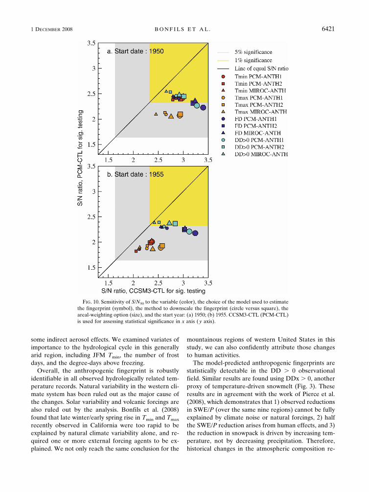
In this section, we examine the sensitivity of ourD&A results to a range of different processing choices.We find that the ANTH fingerprint can be positivelyidentified in all four observed temperature indices, ir-respective of the model used to estimate the fingerprint(two options) or the noise (two options), the methodused to downscale the PCM fingerprint (two options),the end points values, and the applied areal weighting(two options; see Fig. 10). The weighting option, whichhas not been discussed previously, involves either unitweighting or appropriate areal weighting of the ninemountain regions.

In all 48 cases, the detection time for an anthropo-genic fingerprint occurs as early as 1986 and no laterthan 1994. The S/N50 results are sensitive to the noiseconfiguration. In Fig. 10, all symbols are located to theright of the line of equal S/N ratio, indicating that S/N50

(as well as detection time) is always enhanced when theCCSM3-CTL run is used for assessing statistical signifi-cance. This systematic difference in S/N50 ratios is dueto the larger decadal variability in the PCM-CTL run(Pierce et al. 2008). The sensitivity of S/N50 values tothe choice of downscaling method and model used toestimate the fingerprint is much smaller than the sen-sitivity to the noise configuration (Fig. 10).

For the Tmin results with no areal weighting, the lead-ing signal and noise modes show comparatively littlespatial structure (Figs. 8a,b). Because of this, the Tmin

S/N50 results are relatively insensitive to the area-

weighting option. In the FD and DD � 0 cases, how-ever, the dominant signal and noise modes have morepronounced spatial structures (Figs. 8c,d), and henceS/N50 values are more sensitive to the applied weighting(Fig. 10). Interestingly, S/N50 values obtained for Tmin

are higher than those obtained for Tmax, irrespective ofthe various processing options. The results are consis-tent with the detection results obtained by Bonfils et al.(2008) over the domain of California.

We also considered whether our results were sensi-tive to the choice of later start dates (1955, 1960, and1965). For a 1955 start date, anthropogenic effects ontemperature are consistently identifiable, independentof processing choices (see Fig. 10b). For later startdates, however (1960 and 1965), consistent detection isnot achieved. This is primarily because of an increase innoise and degradation in S/N ratios when trends arecalculated over shorter periods of time (see, e.g., Santeret al. 2007).

5. Discussion and conclusions

In this work we have assessed whether observedwarming in the western United States over the period1950–99 is both outside the range expected because ofnatural internal climate variability and consistent withthe expected effects of anthropogenic climate forcing.This was done with a model-estimated anthropogenic“fingerprint” of warming that includes the effects ofwell-mixed greenhouse gases, ozone, and direct and

FIG. 9. Time-dependent S/N ratios estimates for Tmin, using CCSM3-CTL for statistical significance testing, and three differentensemble-means for estimating the ANTH fingerprint (unweighted case). Detection time (see arrow, estimated when S/N exceeds andremains above the 5% significance level) is 1986, irrespective of the choice of model used to estimate the fingerprint. The x axisrepresents the last year of L-length linear trend in the signal estimate (with 1950 as the first year).


Fig 9 live 4/C

some indirect aerosol effects. We examined variates ofimportance to the hydrological cycle in this generallyarid region, including JFM Tmin, the number of frostdays, and the degree-days above freezing.

Overall, the anthropogenic fingerprint is robustlyidentifiable in all observed hydrologically related tem-perature records. Natural variability in the western cli-mate system has been ruled out as the major cause ofthe changes. Solar variability and volcanic forcings arealso ruled out by the analysis. Bonfils et al. (2008)found that late winter/early spring rise in Tmin and Tmax

recently observed in California were too rapid to beexplained by natural climate variability alone, and re-quired one or more external forcing agents to be ex-plained. We not only reach the same conclusion for the

mountainous regions of western United States in thisstudy, we can also confidently attribute those changesto human activities.

The model-predicted anthropogenic fingerprints arestatistically detectable in the DD � 0 observationalfield. Similar results are found using DDx � 0, anotherproxy of temperature-driven snowmelt (Fig. 3). Theseresults are in agreement with the work of Pierce et al.(2008), which demonstrates that 1) observed reductionsin SWE/P (over the same nine regions) cannot be fullyexplained by climate noise or natural forcings, 2) halfthe SWE/P reduction arises from human effects, and 3)the reduction in snowpack is driven by increasing tem-perature, not by decreasing precipitation. Therefore,historical changes in the atmospheric composition re-

FIG. 10. Sensitivity of S/N50 to the variable (color), the choice of the model used to estimatethe fingerprint (symbol), the method to downscale the fingerprint (circle versus square), theareal-weighting option (size), and the start year: (a) 1950; (b) 1955. CCSM3-CTL (PCM-CTL)is used for assessing statistical significance in x axis (y axis).


Fig 10 live 4/C

sult in a human-induced warming over western U.S.mountainous regions, itself responsible for the ob-served reductions of snowpack (Pierce et al. 2008) andshifts in the timing of the streamflow (Hidalgo et al.2008, manuscript submitted to J. Climate). Models ofclimate change unanimously project an acceleration ofthe warming in the western United States with tem-perature change projections of �1°–3°C for 2050 and2°–6°C by 2100 in California (Lobell et al. 2006). Withsuch substantial warming, serious implications for wa-ter infrastructure and water supply sustainability can beexpected over the western United States in the nearfuture.

Acknowledgments. First, we thank our three anony-mous reviewers for their thorough reading and theirvery helpful suggestions. This work was performed un-der the auspices of the U.S. Department of Energy byLawrence Livermore National Laboratory under Con-tract DE-AC52-07NA27344. The MIROC data weregenerously supplied by National Institute for Environ-mental Studies Onogawa, Tsukuba, Ibaraki, Japan.The PCM simulation had been made available by theNational Center for Atmospheric Research. Observeddaily maximum and minimum temperature were ob-tained from the University of Washington Land Sur-face Hydrology Research group (http://www.hydro.washington.edu), and the network stations used to gen-erate this dataset were kindly provided by Alan Ham-let. Scripps Institution of Oceanography (SIO) partici-pants, GB and AM, as well as travel costs were sup-ported by LLNL through LDRD grants. BS wassupported by DOE-W-7405-ENG-48 to the Programof Climate Model Diagnoses and Intercomparison(PCMDI). Thanks are also due to Department of En-ergy, which supported TPB as part of the InternationalDetection and Attribution Group (IDAG). CB wasmainly supported by the Distinguished Scientist Fel-lowship awarded to Benjamin Santer in 2005 by theU.S. Department of Energy, Office of Biological andEnvironmental Research. The California Energy Com-mission provided partial salary support for DP and HHat SIO.

REFERENCES

Alexander, M., and Coauthors, 2006: Extratropical atmosphere–ocean variability in CCSM3. J. Climate, 19, 2496–2525.

Andreadis, K. M., and D. P. Lettenmaier, 2006: Assimilating re-motely sensed snow observations into a macroscale hydrol-ogy model. Adv. Water Res., 29, 872–886.

Bala, G., and Coauthors, 2008: Evaluation of a CCSM3 simulationwith a finite volume dynamical core for the atmosphere at 1°latitude � 1.25° longitude resolution. J. Climate, 21, 1467–1486.

Barnett, T. P., and Coauthors, 2008: Human-induced changes inthe hydrology of the western United States. Science, 319,1080–1083.

Bonfils, C., and D. Lobell, 2007: Empirical evidence for a recentslowdown in irrigation-induced cooling. Proc. Natl. Acad. Sci.USA, 104, 13 582–13 587.

——, P. Duffy, B. Santer, T. Wigley, D. B. Lobell, T. J. Phillips,and C. Doutriaux, 2008: Identification of external influenceson temperatures in California. Climatic Change, 87, 43–55.

Cayan, D. R., 1996: Interannual climate variability and snowpackin the western United States. J. Climate, 9, 928–948.

—— K. T. Redmond, and L. G. Riddle, 1999: ENSO and hydro-logic extremes in the western United States. J. Climate, 12,2881–2893.

——, S. A. Kammerdiener, M. D. Dettinger, J. M. Caprio, andD. H. Peterson, 2001: Changes in the onset of spring in thewestern United States. Bull. Amer. Meteor. Soc., 82, 399–415.

Cherkauer, K. A., and D. P. Lettenmaier, 2003: Simulation of spa-tial variability in snow and frozen soil. J. Geophys. Res., 108,8858, doi:10.1029/2003JD003575.

Christidis, N., P. A. Stott, S. Brown, D. J. Karoly, and J. Caesar,2007: Human contribution to the lengthening of the growingseason during 1950–99. J. Climate, 20, 5441–5454.

Collins, W. D., and Coauthors, 2006: The Community ClimateSystem Model version 3 (CCSM3). J. Climate, 19, 2122–2143.

DeGaetano, A. T., and R. J. Allen, 2002: Trends in 20th centurytemperature extremes across the United States. J. Climate,15, 3188–3205.

Dettinger, M. D., and D. R. Cayan, 1995: Large-scale atmosphericforcing of recent trends toward early snowmelt runoff in Cali-fornia. J. Climate, 8, 606–623.

Gedney, N., P. M. Cox, R. A. Betts, O. Boucher, C. Huntingford,and P. A. Stott, 2006: Detection of a direct carbon dioxideeffect in continental river runoff records. Nature, 439, 835–838.

Gillett, N. P., and A. J. Weaver, 2004: Detecting the effect of cli-mate change on Canadian forest fires. Geophys. Res. Lett., 31,L18211, doi:10.1029/2004GL020876.

——, R. J. Allan, and T. J. Ansell, 2005: Detection of externalinfluence on sea level pressure with a multi-model ensemble.Geophys. Res. Lett., 32, L19714, doi:10.1029/2005GL023640.

Gleick, P. H., and Coauthors, 2000: Water: The potential conse-quences of climate variability and change for the water re-sources of the United States. The Report of the Water SectorAssessment Team of the National Assessment of the Poten-tial Consequences of Climate Variability and Change, 160 pp.

Groisman, P. Ya., T. R. Karl, R. W. Knight, and G. L. Stenchikov,1994: Changes of snow cover, temperature, and radiative heatbalance over the Northern Hemisphere. J. Climate, 7, 1633–1656.

Hamlet, A. F., and D. P. Lettenmaier, 2005: Production of tem-porally consistent gridded precipitation and temperaturefields for the continental United States. J. Hydrometeor., 6,330–336.

Hasselmann, K., 1979: On the signal-to-noise problem in atmo-spheric response studies. Meteorology of Tropical Oceans, D.B. Shaw, Ed., Royal Meteorological Society of London, 251–259.

Hayhoe, K., and Coauthors, 2004: Emissions pathways, climatechange, and impacts on California. Proc. Natl. Acad. Sci.USA, 101, 12 422–12 427.

Hidalgo, H. G., M. D. Dettinger, and D. R. Cayan, 2008: Down-scaling with constructed analogues: Daily precipitation and


temperature fields over the United States. California EnergyCommission Rep. CEC-500-2007-123, 62 pp.

——, and Coauthors, 2008: Detection and attribution of climatechange in streamflow timing of the western United States. J.Climate, submitted.

K-1 model developers, 2004: K-1 Coupled GCM (MIROC) de-scription. H. Hasumi and S. Emori, Eds., Center for ClimateSystem Research, University of Tokyo, 38 pp.

Kalnay, E., and Coauthors, 1996: The NCEP/NCAR 40-Year Re-analysis Project. Bull. Amer. Meteor. Soc., 77, 437–471.

Karl, T. R., C. N. Williams Jr., P. J. Young, and W. M. Wendland,1986: A model to estimate the time of observation bias asso-ciated with monthly mean maximum, minimum, and meantemperature for the United States. J. Climate Appl. Meteor.,25, 145–160.

——, ——, F. T. Quinlan, and T. A. Boden, 1990: United StatesHistorical Climatology Network (HCN) serial temperatureand precipitation data. Environmental Science Division, Pub-lication 3404, Carbon Dioxide Information and AnalysisCenter, Oak Ridge National Laboratory, Oak Ridge, TN, 389pp.

Karoly, D. J., and Q. Wu, 2005: Detection of regional surfacetemperature trends. J. Climate, 18, 4337–4343.

——, K. Braganza, P. A. Stott, J. M. Arblaster, G. A. Meehl, A. J.Broccoli, and K. W. Dixon, 2003: Detection of a human in-fluence on North American climate. Science, 302, 1200–1203.

Knowles, N., M. D. Dettinger, and D. R. Cayan, 2006: Trends insnowfall versus rainfall in the western United States. J. Cli-mate, 19, 4545–4559.

Lambert, F. H., N. P. Gillett, D. A. Stone, and C. Huntingford,2005: Attribution studies of observed land precipitationchanges with nine coupled models. Geophys. Res. Lett., 32,L18704, doi:10.1029/2005GL023654.

Liang, X., D. P. Lettenmaier, E. F. Wood, and S. J. Burges, 1994:A simple hydrologically based model of land surface waterand energy fluxes for general circulation models. J. Geophys.Res., 99, 14 415–14 428.

Linsley, R. K., Jr., 1943: A simple procedure for the day-to-dayforecasting of runoff from snowmelt. Trans. Amer. Geophys.Union, 24, 719–736.

Lobell, D., C. Field, K. Nicholas-Cahill, and C. Bonfils, 2006:Impacts of future climate change on California perennialcrop yields: Model projections with climate and crop uncer-tainties. Agric. For. Meteor., 141, 208–218.

Mantua, N. J., S. R. Hare, Y. Zhang, J. M. Wallace, and R. C.Francis, 1997: A Pacific interdecadal climate oscillation withimpacts on salmon production. Bull. Amer. Meteor. Soc., 78,1069–1079.

Maurer, E. P., and H. G. Hidalgo, 2007: Utility of daily vs.monthly large-scale climate data: An intercomparison of twostatistical downscaling methods. Hydrol. Earth Syst. Sci., 12,551–563.

——, I. T. Stewart, C. Bonfils, P. B. Duffy, and D. Cayan, 2007:Detection, attribution, and sensitivity of trends toward earlierstreamflow in the Sierra Nevada. J. Geophys. Res., 112,D11118, doi:10.1029/2006JD008088.

Meehl, G. A., and A. Hu, 2006: Megadroughts in the Indian mon-soon region and southwest North America and a mechanismfor associated multidecadal Pacific sea surface temperatureanomalies. J. Climate, 19, 1605–1623.

——, ——, and B. D. Santer, 2009: The mid-1970s climate shift inthe Pacific and the relative roles of forced versus inherentdecadal variability. J. Climate, in press.

Milly, P. C. D., J. Betancourt, M. Falkenmark, R. M. Hirsch,Z. W. Kundzewicz, D. P. Lettenmaier, and R. J. Stouffer,2008: Stationarity is dead: Whither water management? Sci-ence, 319, 573–574.

Mote, P. W., 2006: Climate-driven variability and trends in moun-tain snowpack in western North America. J. Climate, 19,6209–6220.

——Mote, P. W., A. F. Hamlet, M. P. Clark, and D. P. Letten-maier, 2005: Declining mountain snowpack in western NorthAmerica. Bull. Amer. Meteor. Soc., 86, 39–49.

Nozawa, T., T. Nagashima, T. Ogura, T. Yokohara, N. Okada, andH. Shiogama, 2007: Climate change simulations with acoupled ocean–atmosphere GCM called the Model for Inter-disciplinary Research on Climate: MIROC. CGER’s Super-computer Monograph Rep. Vol. 12, Center for Global Envi-ronmental Research, National Institute for EnvironmentalStudies, Japan, 93 pp.

Pierce, D. W., and Coauthors, 2008: Attribution of declining west-ern U.S. snowpack to human effects. J. Climate, 21, 6425–6444.

Press, W. H., B. P. Flannery, S. A. Teukolsky, and W. T. Vetter-ling, 1992: Kolmogorov-Smirnov test. Numerical Recipes inFORTRAN: The Art of Scientific Computing. 2nd ed. Cam-bridge University Press, 617–620.

Santer, B. D., and T. M. L. Wigley, 2008: Progress in detection andattribution research. Climatic Change Science and Policy, S.H. Schneider, A. Rosencranz, and M. D. Mastrandrea, Eds.,Island Press, in press.

——, U. Mikolajewicz, W. Brüggemann, U. Cubasch, K. Hassel-mann, H. Höck, E. Maier-Reimer, and T. M. L. Wigley, 1995:Ocean variability and its influence on the detectability ofgreenhouse warming signals. J. Geophys. Res., 100, 10 693–10 725.

——, T. M. L. Wigley, J. S. Boyle, D. J. Gaffen, J. J. Hnilo, D.Nychka, D. E. Parker, and K. E. Taylor, 2000a: Statisticalsignificance of trends and trend differences in layer-averageatmospheric temperature time series. J. Geophys. Res., 105,7337–7356.

——, and Coauthors, 2000b: Interpreting differential temperaturetrends at the surface and in the lower troposphere. Science,287, 1227–1232.

——, and Coauthors, 2007: Identification of human-inducedchanges in atmospheric moisture content. Proc. Natl. Acad.Sci. USA, 104, 15 248–15 253.

Shindell, D. T., G. A. Schmidt, R. L. Miller, and D. Rind, 2001:Northern Hemisphere winter climate response to greenhousegas, ozone, solar, and volcanic forcing. J. Geophys. Res., 106,7193–7210.

Shiogama, H., M. Watanabe, M. Kimoto, and T. Nozawa, 2005:Anthropogenic and natural forcing impacts on ENSO-likedecadal variability during the second half of the 20th century.Geophys. Res. Lett., 32, L21714, doi:10.1029/2005GL023871.

Smith, S. R., and J. J. O’Brien, 2001: Regional snowfall distribu-tions associated with ENSO: Implications for seasonal fore-casting. Bull. Amer. Meteor. Soc., 82, 1179–1191.

Stewart, I. T., D. R. Cayan, and M. D. Dettinger, 2005: Changestoward earlier streamflow timing across western NorthAmerica. J. Climate, 18, 1136–1155.

Stott, P. A., 2003: Attribution of regional-scale temperaturechanges to anthropogenic and natural causes. Geophys. Res.Lett., 30, 1728, doi:10.1029/2003GL017324.

Vose, R. S., C. N. Williams, Jr., T. C. Peterson, T. R. Karl, and


D. R. Easterling, 2003: An evaluation of the time of obser-vation bias adjustment in the U.S. Historical ClimatologyNetwork. Geophys. Res. Lett., 30, 2046, doi:10.1029/2003GL018111.

Washington, W. M., and Coauthors, 2000: Parallel Climate Model(PCM) control and transient simulations. Climate Dyn., 16,755–774.

Westerling, A. L., H. G. Hidalgo, D. R. Cayan, and T. W. Swet-nam, 2006: Warming and earlier spring increase western U.S.forest wildfire activity. Science, 313, 940–943.

Willett, K. M., N. P. Gillett, P. D. Jones, and P. W. Thorne, 2007:

Attribution of observed surface humidity changes to humaninfluence. Nature, 449, 710–712.

Wood, A. W., L. R. Leung, V. Sridhar, and D. P. Lettenmaier,2004: Hydrologic implications of dynamical and statistical ap-proaches to downscaling climate model outputs. ClimaticChange, 62, 189–216.

Zhang, X., F. W. Zwiers, G. C. Hegerl, F. H. Lambert, N. P.Gillett, S. Solomon, P. A. Stott, and T. Nozawa, 2007: Detec-tion of human influence on twentieth-century precipitationtrends. Nature, 448, 461–465.

Zwiers, F. W., and X. Zhang, 2003: Towards regional climatechange detection. J. Climate, 16, 793–797.


detection and attribution of temperature changes in...

Documents