University of WaterlooCenter for Theoretical Neuroscience

Detecting Shapes in Raven’s Matrices

Author:

Jacqueline Mok

Supervisors:

Chris Eliasmith, Charlie Tang

April 30, 2010

Table of Contents

1.0 Introduction . . . . . . . . . . . . . . . . . . . . . . . . . . . . . . . . . . . . . . . . . . . . 1

2.0 Background and Related Work . . . . . . . . . . . . . . . . . . . . . . . . . . . . . . . . 2

3.0 Results . . . . . . . . . . . . . . . . . . . . . . . . . . . . . . . . . . . . . . . . . . . . . . . 2

3.1 Overview . . . . . . . . . . . . . . . . . . . . . . . . . . . . . . . . . . . . . . . . . . . . . . . 2

3.2 Code Details . . . . . . . . . . . . . . . . . . . . . . . . . . . . . . . . . . . . . . . . . . . . . 3

3.3 Sift raven.m . . . . . . . . . . . . . . . . . . . . . . . . . . . . . . . . . . . . . . . . . . . . . . 3

3.4 Hough.m . . . . . . . . . . . . . . . . . . . . . . . . . . . . . . . . . . . . . . . . . . . . . . . . 5

3.5 Cluster.m . . . . . . . . . . . . . . . . . . . . . . . . . . . . . . . . . . . . . . . . . . . . . . . 10

4.0 Examples and Theoretical Adaptation to Rasmussen’s Model . . . . . . . . . . . . . . 12

4.1 Basic Idea . . . . . . . . . . . . . . . . . . . . . . . . . . . . . . . . . . . . . . . . . . . . . . . 12

4.2 Example 1 . . . . . . . . . . . . . . . . . . . . . . . . . . . . . . . . . . . . . . . . . . . . . . . 12

4.3 Example 2 . . . . . . . . . . . . . . . . . . . . . . . . . . . . . . . . . . . . . . . . . . . . . . . 15

5.0 Conclusion . . . . . . . . . . . . . . . . . . . . . . . . . . . . . . . . . . . . . . . . . . . . . 17

5.1 Summary of Contributions . . . . . . . . . . . . . . . . . . . . . . . . . . . . . . . . . . . . . . 17

5.2 Future Problems . . . . . . . . . . . . . . . . . . . . . . . . . . . . . . . . . . . . . . . . . . . 17

References . . . . . . . . . . . . . . . . . . . . . . . . . . . . . . . . . . . . . . . . . . . . . . . . 20

Appendix A - Sift raven.m . . . . . . . . . . . . . . . . . . . . . . . . . . . . . . . . . . . . . . 21

Appendix B - Hough.m . . . . . . . . . . . . . . . . . . . . . . . . . . . . . . . . . . . . . . . . 23

Appendix C - Cluster.m . . . . . . . . . . . . . . . . . . . . . . . . . . . . . . . . . . . . . . . . 29

Appendix D - Plot thresholds.m . . . . . . . . . . . . . . . . . . . . . . . . . . . . . . . . . . . 30

i

List of Figures

Figure 1 — Sample Figures from Raven’s Matrices . . . . . . . . . . . . . . . . . . . . . . . . . . 1

Figure 2 — Matched keypoints from image to dashed line. . . . . . . . . . . . . . . . . . . . . . 3

Figure 3 — Siftmatch results and threshold . . . . . . . . . . . . . . . . . . . . . . . . . . . . . . 4

Figure 4 — Translation of model points (right) to image points (left). . . . . . . . . . . . . . . . 8

Figure 5 — Results for clustering . . . . . . . . . . . . . . . . . . . . . . . . . . . . . . . . . . . 9

Figure 6 — Plot of x and y radii versus number of clusters . . . . . . . . . . . . . . . . . . . . . 10

Figure 7 — Errors from clustering . . . . . . . . . . . . . . . . . . . . . . . . . . . . . . . . . . . 11

Figure 8 — Raven Matrix 1 and Databank . . . . . . . . . . . . . . . . . . . . . . . . . . . . . . 12

Figure 9 — Raven Matrix 6 and Databank . . . . . . . . . . . . . . . . . . . . . . . . . . . . . . 15

Figure 10 — Image with one small triangle (left) and two small triangles combined (right). . . . 18

ii

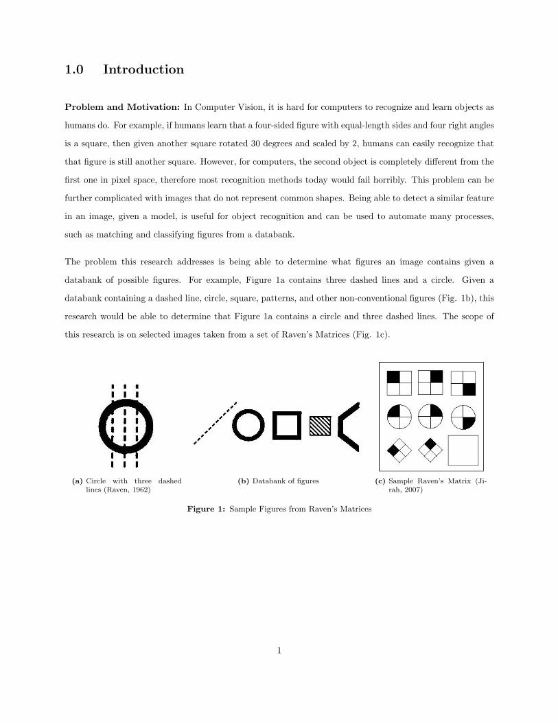
1.0 Introduction

Problem and Motivation: In Computer Vision, it is hard for computers to recognize and learn objects as

humans do. For example, if humans learn that a four-sided figure with equal-length sides and four right angles

is a square, then given another square rotated 30 degrees and scaled by 2, humans can easily recognize that

that figure is still another square. However, for computers, the second object is completely different from the

first one in pixel space, therefore most recognition methods today would fail horribly. This problem can be

further complicated with images that do not represent common shapes. Being able to detect a similar feature

in an image, given a model, is useful for object recognition and can be used to automate many processes,

such as matching and classifying figures from a databank.

The problem this research addresses is being able to determine what figures an image contains given a

databank of possible figures. For example, Figure 1a contains three dashed lines and a circle. Given a

databank containing a dashed line, circle, square, patterns, and other non-conventional figures (Fig. 1b), this

research would be able to determine that Figure 1a contains a circle and three dashed lines. The scope of

this research is on selected images taken from a set of Raven’s Matrices (Fig. 1c).

(a) Circle with three dashedlines (Raven, 1962)

(b) Databank of figures (c) Sample Raven’s Matrix (Ji-rah, 2007)

Figure 1: Sample Figures from Raven’s Matrices

1

2.0 Background and Related Work

This research uses the Scale-Invariant Feature Transform (SIFT) (Lowe, 2004) technique to match keypoints

from a model to an image by providing the location, scale, and orientation of the matching keypoints. E.g.,

in a square, the main keypoints detected would include the four corners. Using an implementation of SIFT

by Vedaldi (2006), the matched keypoints can be obtained (as in Fig. 2). The figures from each image in

Raven’s Matrices can then be extracted using additional techniques proposed in this work.

This research uses the SIFT approach because SIFT is a very robust technique that can detect key features

regardless of its orientation, scale, or location.

3.0 Results

3.1 Overview

The SIFT implementation detects and matches keypoint between a test and a model image, but it does

not determine which model from the databank is best for a particular Raven image. This research applies

the Hough transform (Ballard, 1981) on the results of the keypoint matches between a Raven image and

a model. The Hough transform is based on a voting procedure, where each keypoint match in the Raven

image goes through the entire databank and votes for the possible models that it could contain. The most

popular candidate from the databank would be declared the winner, indicating that the model is present in

the image. Afterwards, an affine transformation is applied to find the best fit for the model onto the image.

This method would be able to determine where, in a particular image, the model is located. Furthermore,

the scale and orientation will also be known. In some cases, there may be more than one figure from the

databank that is present in the image (refer to Fig. 1a). In these situations, several candidates from the

databank would be very popular, and hence multiple winners would be declared. In other cases, the model

may appear more than once in the image, so a clustering technique would be used to detect that the model

appears more than once.

Afterwards, an affine transformation is applied to find the best fit for the model onto the image. This method

would be able to determine where, in a particular image, the model is located. Furthermore, the scale and

2

orientation will also be known. In some cases, there may be more than one figure from the databank that is

present in the image (refer to Fig. 1a and Fig. 2). In these situations, several candidates from the databank

would be very popular, and hence multiple winners would be declared.

3.2 Code Details

Figure 2: Matched keypoints from imageto dashed line.

The given set of Raven’s Matrices set is separated into 36 different

folders named ’ravenx’, where x is the number of each matrix.

Each of the 8 cells in each matrix is cropped and put in their

corresponding folder.

The training set is created by extracting specific figures from exist-

ing cells (e.g. from Fig. 1a, one training model is a circle, another

is a dashed line). It was later discovered that having images too

close to the border impacts SIFT’s ability to extract keypoint de-

scriptors, so an abundance of space was left between each image

or model and its boundary.

3.3 Sift raven.m

In this Matlab file, the script runs through each of the eight cell images (test images) from every Raven matrix

and applies SIFT and the Hough transform on each test and model pair. To apply the SIFT technique, the

function sift() is called twice, once for the test image and once for the model, given the following parameters:

• image - the image on which sift() will extract keypoint descriptors• threshold - value such that the maxima of the Difference of Gaussian scale space below this threshold

are ignored (Vedaldi, 2006)• edge threshold - localization threshold• boundary point - remove points whose descriptor intersects the boundary

sift() returns two vectors. The first vector contains the image’s frames, representing the location, scale,

and orientation of the keypoint descriptor. The second vector is a 128-dimensional vector representing the

descriptors. More information can be found in Vedaldi’s SIFT documentation.

3

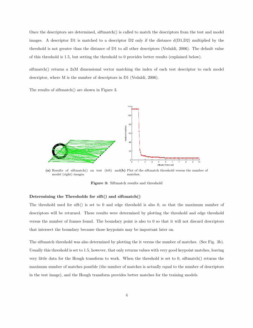
Once the descriptors are determined, siftmatch() is called to match the descriptors from the test and model

images. A descriptor D1 is matched to a descriptor D2 only if the distance d(D1,D2) multiplied by the

threshold is not greater than the distance of D1 to all other descriptors (Vedaldi, 2006). The default value

of this threshold is 1.5, but setting the threshold to 0 provides better results (explained below).

siftmatch() returns a 2xM dimensional vector matching the index of each test descriptor to each model

descriptor, where M is the number of descriptors in D1 (Vedaldi, 2006).

The results of siftmatch() are shown in Figure 3.

(a) Results of siftmatch() on test (left) andmodel (right) images.

(b) Plot of the siftmatch threshold versus the number ofmatches.

Figure 3: Siftmatch results and threshold

Determining the Thresholds for sift() and siftmatch()

The threshold used for sift() is set to 0 and edge threshold is also 0, so that the maximum number of

descriptors will be returned. These results were determined by plotting the threshold and edge threshold

versus the number of frames found. The boundary point is also to 0 so that it will not discard descriptors

that intersect the boundary because those keypoints may be important later on.

The siftmatch threshold was also determined by plotting the it versus the number of matches. (See Fig. 3b).

Usually this threshold is set to 1.5, however, that only returns values with very good keypoint matches, leaving

very little data for the Hough transform to work. When the threshold is set to 0, siftmatch() returns the

maximum number of matches possible (the number of matches is actually equal to the number of descriptors

in the test image), and the Hough transform provides better matches for the training models.

4

After SIFT has been applied, hough() is called to apply the Hough transform on the keypoint matches.

3.4 Hough.m

The Hough transform is a feature extraction technique used in image analysis, computer vision, and digital

image processing (Shapiro and Stockman, 2001), and it is based on a voting procedure. For example, given a

circle (test image), and a databank containing a square, circle, and semi-circle (model images), each keypoint

descriptor on the circle would vote for the possible model images from the databank. Most likely the circle

model, and not the semi circle or square, would acquire the most votes from all the descriptors, and so

it would be declared the “winner”, meaning a circle exists in the test image. More information about the

Hough transform can also be found in David Lowe’s article, Distinctive Image Features from Scale-Invariant

Keypoints.

In the hough() function, the Hough transform is applied in a similar way. Given a set of keypoint matches

between the test and model images in the image space, each match will vote for a certain bin in the Hough

space (a bin describes the (x,y) location, scale, and orientation of the descriptor). After all the keypoints

have voted, the bin with the greatest number of votes will provide the most accurate information about the

location, scale, and orientation of the model relative to the test image.

hough() takes the following parameters:

• matches - keypoint matches between the image and model produced by siftmatch()• test frames, model frames - the test and model frames containing the (x,y) location, scale, and orien-

tation of the descriptors• model name - name of the model, for convenience• cell, model - the test and model images used for plotting

The output of hough() contains the following:

• (x,y) location of where the model is located on the test image,• scale of model relative to the test image,• orientation of the model relative to the test image,• a number of figures or plots that will be described below, OR• ’no matches’ if there are no matches between the test and model image

5

Variables

• distinct indices - stores the indices of each bin in a hash table

Each bin describes four dimensions, listed below:

• BW x: x-bin width• BW y: y-bin width• BW scale: each partition is the range between two consecutive numbers in this vector• BW theta: bin width for orientation in radians

• test uv, model xy - vectors used for affine fitting• best count: bin with the greatest count• winning bin: bin containing the most votes

Explanation of Code

For each pair of matches passed in, the test and model frames are extracted into test params and model params.

Then a transformation is applied to determine the transformation from the center of the model to the test

image. The change in scale and orientation is calculated as follows:

∆scale =test scale

model scale

∆θ = test orientation−model orientation

The transformation is calculated as follows:

x

y

1

=

∆scale× cos(∆θ) −sin(∆θ) xt

sin(∆θ) ∆scale× cos(∆θ) yt

0 0 1

×−xm + model width

2

−ym + model height2

1

x and y represent where the center of the model image is mapped on the test image, and the subscripts t and

m refer to the test and model descriptors.

The bins for the each dimension (bin x, bin y, bin scale, bin theta) are determined using the above infor-

mation. Checks were made to ensure that there are no negative values for orientation, since negative values

would be a duplicate other values (periodic property).

6

According to Lowes Distinctive Image Features from Scale-Invariant Keypoints, every descriptor should vote

for the two closest bins in each dimension, resulting in 16 votes per descriptor. To do this, the floor and

ceiling are taken from each dimension, and the bin values for each of the 16 votes are stored in permut.

Next the hash index for each bin is computed using serialization by calling get hash ind(), and the indices

of the matches are stored in the hash table. For example, if 100 matches are passed in as a parameter to

hough(), and the 10th pair matched the 4th test descripter with the 9th model descriptor, then the index 10

would be stored in the hash table at the computed index. This is considered one vote in the hash table. The

bin with the greatest number of votes is tracked using best count and winning bin.

Clustering Section

This section determines if clustering should be performed. If the bin with the greatest number of votes (the

first bin) contains at least three keypoint matches (i.e. the model is found in the test image), then the model

could exist multiples times in the test image (see Fig. 1a). In that case, this section will proceed with

clustering. However, if the first bin has too few keypoint matches (i.e. the model does not exist in the test

image), then the clustering function, cluster(), will not be called.

Variables

• X, Y, S, and T are vectors that store the mean (x,y) values, scale, and orientation (radians) taken from

the keypoints found in each bin. Tx and Ty represent the orientation on the unit circle.• allX and allY store all the x and y values mapped from the model to the test image (these values are

a collection from all 30 bins) - it is helpful later on as a diagnostic test to visualize where the clusters

may lie.• firsthasmatch - this is a flag that determines if the first bin found a match between the model and the

test image

Explanation of Code

If there exists some keypoint matches between the test and model image, the size of each bin is stored in vec,

and sorted in descending order to find out which bin has the most tallies. The number of votes in each bin

is stored in sorted bin size, and the index into vec is stored in sorted bin size ind.

The code runs through the top 30 bins (NBin), and for each bin it retrieves the index of the nth bin, the

7

indices representing the matches in that bin, and stores all the x and y values from the test and model frames

into test uv and model xy. These two vectors are used for affine fitting to determine accurate parameters for

mapping the model points to the test points.

The equation used for affine fitting is the following (Lowe, 2004):

x y 0 0 1 0

0 0 x y 0 1

. . .

. . .

×

m1

m2

m3

m4

lx

ly

=

u

v

...

,m =

m1

m2

m3

m4

lx

ly

x and y represent the location for each model point, and u and v represent the test points. mi represent the

parameters that rotate, scale, and stretch the model points. lx and ly represent the model translation (Lowe,

2004).

The vector m is calculated using Matlab’s pinv function instead of the backslash operator because the

backslash operator often produced unpredictable results for m.

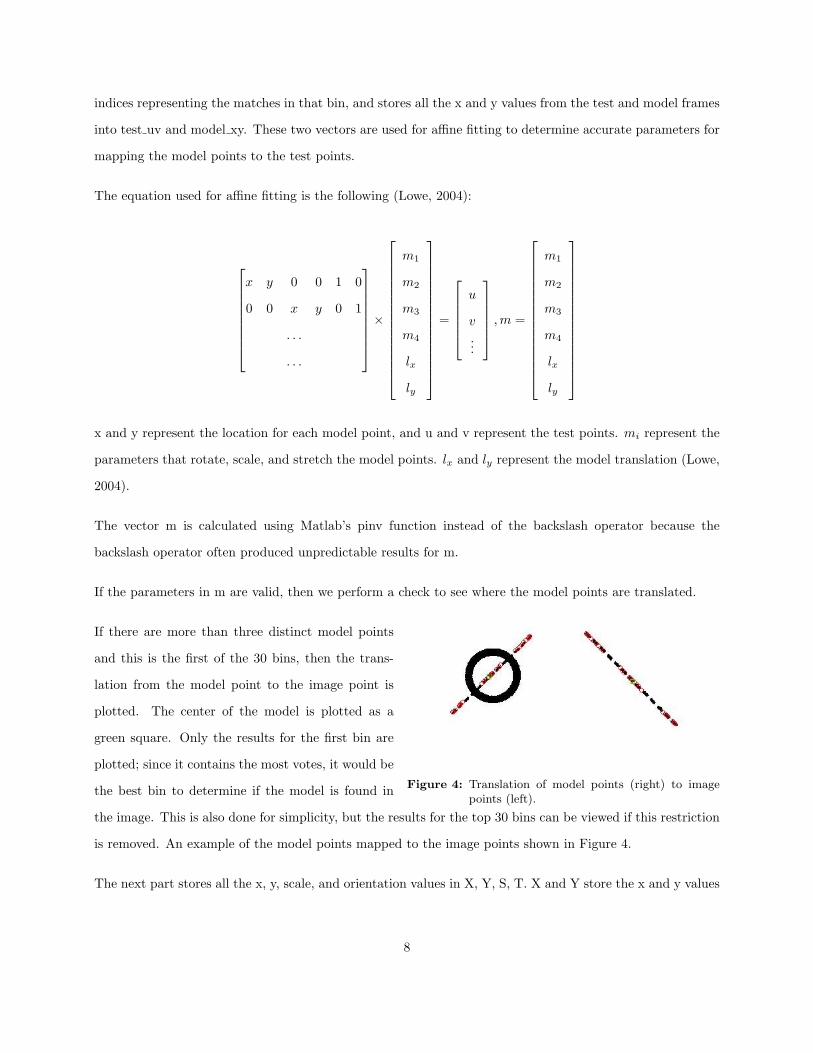
If the parameters in m are valid, then we perform a check to see where the model points are translated.

Figure 4: Translation of model points (right) to imagepoints (left).

If there are more than three distinct model points

and this is the first of the 30 bins, then the trans-

lation from the model point to the image point is

plotted. The center of the model is plotted as a

green square. Only the results for the first bin are

plotted; since it contains the most votes, it would be

the best bin to determine if the model is found in

the image. This is also done for simplicity, but the results for the top 30 bins can be viewed if this restriction

is removed. An example of the model points mapped to the image points shown in Figure 4.

The next part stores all the x, y, scale, and orientation values in X, Y, S, T. X and Y store the x and y values

8

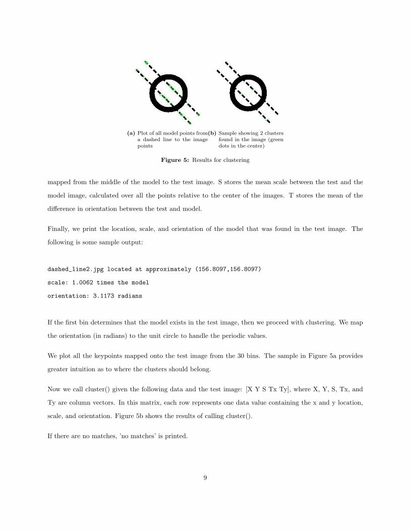
(a) Plot of all model points froma dashed line to the imagepoints

(b) Sample showing 2 clustersfound in the image (greendots in the center)

Figure 5: Results for clustering

mapped from the middle of the model to the test image. S stores the mean scale between the test and the

model image, calculated over all the points relative to the center of the images. T stores the mean of the

difference in orientation between the test and model.

Finally, we print the location, scale, and orientation of the model that was found in the test image. The

following is some sample output:

dashed_line2.jpg located at approximately (156.8097,156.8097)

scale: 1.0062 times the model

orientation: 3.1173 radians

If the first bin determines that the model exists in the test image, then we proceed with clustering. We map

the orientation (in radians) to the unit circle to handle the periodic values.

We plot all the keypoints mapped onto the test image from the 30 bins. The sample in Figure 5a provides

greater intuition as to where the clusters should belong.

Now we call cluster() given the following data and the test image: [X Y S Tx Ty], where X, Y, S, Tx, and

Ty are column vectors. In this matrix, each row represents one data value containing the x and y location,

scale, and orientation. Figure 5b shows the results of calling cluster().

If there are no matches, ’no matches’ is printed.

9

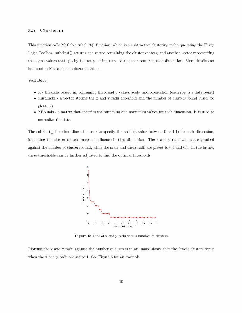
3.5 Cluster.m

This function calls Matlab’s subclust() function, which is a subtractive clustering technique using the Fuzzy

Logic Toolbox. subclust() returns one vector containing the cluster centers, and another vector representing

the sigma values that specify the range of influence of a cluster center in each dimension. More details can

be found in Matlab’s help documentation.

Variables

• X - the data passed in, containing the x and y values, scale, and orientation (each row is a data point)• clust radii - a vector storing the x and y radii threshold and the number of clusters found (used for

plotting)• XBounds - a matrix that specifies the minimum and maximum values for each dimension. It is used to

normalize the data.

The subclust() function allows the user to specify the radii (a value between 0 and 1) for each dimension,

indicating the cluster centers range of influence in that dimension. The x and y radii values are graphed

against the number of clusters found, while the scale and theta radii are preset to 0.4 and 0.3. In the future,

these thresholds can be further adjusted to find the optimal thresholds.

Figure 6: Plot of x and y radii versus number of clusters

Plotting the x and y radii against the number of clusters in an image shows that the fewest clusters occur

when the x and y radii are set to 1. See Figure 6 for an example.

10

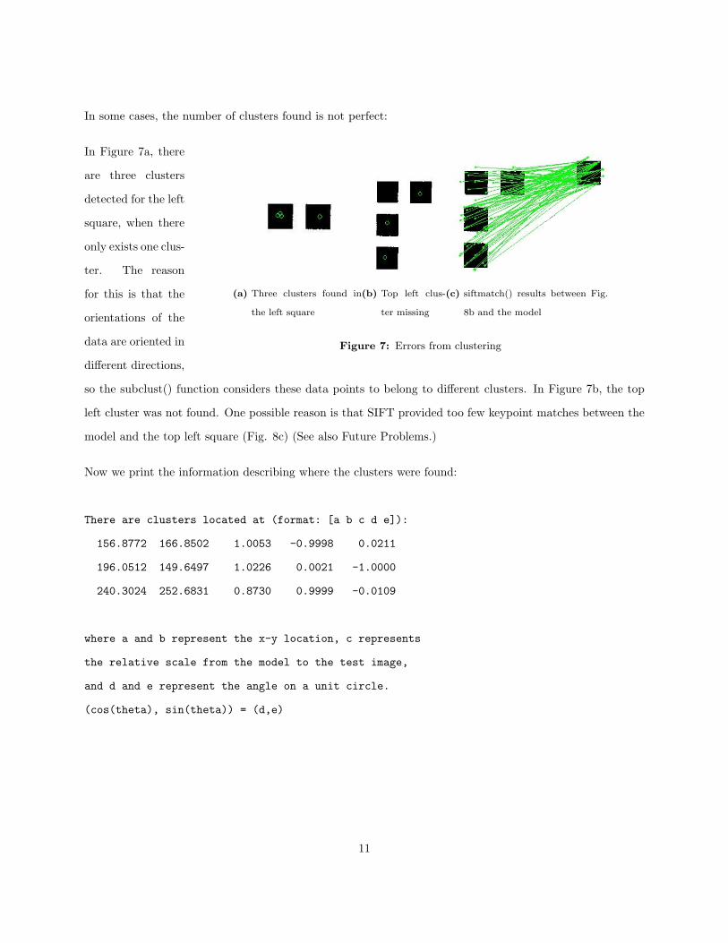
In some cases, the number of clusters found is not perfect:

(a) Three clusters found in

the left square

(b) Top left clus-

ter missing

(c) siftmatch() results between Fig.

8b and the model

Figure 7: Errors from clustering

In Figure 7a, there

are three clusters

detected for the left

square, when there

only exists one clus-

ter. The reason

for this is that the

orientations of the

data are oriented in

different directions,

so the subclust() function considers these data points to belong to different clusters. In Figure 7b, the top

left cluster was not found. One possible reason is that SIFT provided too few keypoint matches between the

model and the top left square (Fig. 8c) (See also Future Problems.)

Now we print the information describing where the clusters were found:

There are clusters located at (format: [a b c d e]):

156.8772 166.8502 1.0053 -0.9998 0.0211

196.0512 149.6497 1.0226 0.0021 -1.0000

240.3024 252.6831 0.8730 0.9999 -0.0109

where a and b represent the x-y location, c represents

the relative scale from the model to the test image,

and d and e represent the angle on a unit circle.

(cos(theta), sin(theta)) = (d,e)

11

4.0 Examples and Theoretical Adaptation to Rasmussen’s Model

The Rasmussen Model, created by Daniel Rasmussen, is a model that provides an algorithm to solve Raven’s

Matrices. The following is a modified version of the Rasmussen input and output, that illustrates how this

research can be adapted to the Rasmussen Model.

4.1 Basic Idea

For each Raven image, apply SIFT and the Hough transform on each of the 8 cells with the models in the

databank. The output would provide information on what models exist in the test cell, and the number of

times that model occurs (clustering). Then a converter would map the Rasmussen input with the output

above. If there is a match, this converter would take the corresponding Rasmussen solution, and apply SIFT

and the Hough transform on the answer cells to determine the image containing the correct answer. This

method shows how solving Raven’s Matrices can be automated using SIFT and the Hough transform to

detect the figures in the Raven image.

The following examples assume that the output from the Hough transform (including clustering) do not

contain the problems discussed above or in the Future Problems section. For example, if there are multiple

clusters found in an image due to a difference in orientation, only one of those clusters would be considered

for the purposes of these examples.

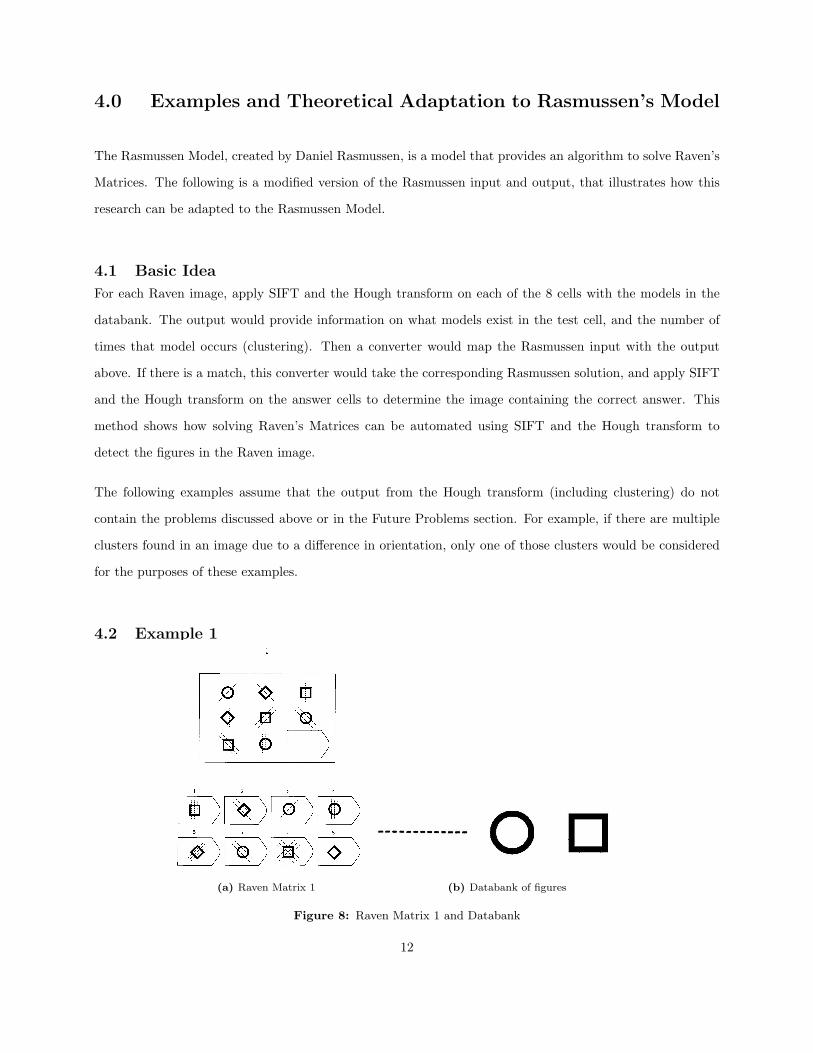
4.2 Example 1

(a) Raven Matrix 1 (b) Databank of figures

Figure 8: Raven Matrix 1 and Databank

12

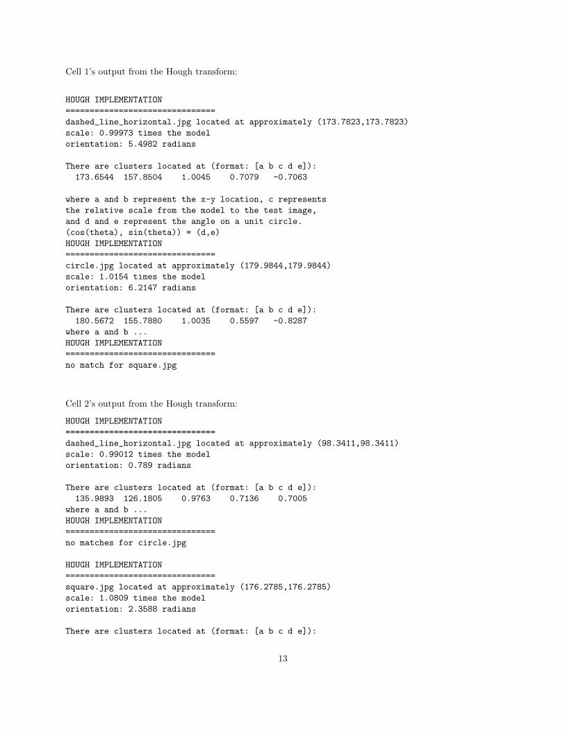
Cell 1’s output from the Hough transform:

HOUGH IMPLEMENTATION===============================dashed_line_horizontal.jpg located at approximately (173.7823,173.7823)scale: 0.99973 times the modelorientation: 5.4982 radians

There are clusters located at (format: [a b c d e]):173.6544 157.8504 1.0045 0.7079 -0.7063

where a and b represent the x-y location, c representsthe relative scale from the model to the test image,and d and e represent the angle on a unit circle.(cos(theta), sin(theta)) = (d,e)HOUGH IMPLEMENTATION===============================circle.jpg located at approximately (179.9844,179.9844)scale: 1.0154 times the modelorientation: 6.2147 radians

There are clusters located at (format: [a b c d e]):180.5672 155.7880 1.0035 0.5597 -0.8287

where a and b ...HOUGH IMPLEMENTATION===============================no match for square.jpg

Cell 2’s output from the Hough transform:

HOUGH IMPLEMENTATION===============================dashed_line_horizontal.jpg located at approximately (98.3411,98.3411)scale: 0.99012 times the modelorientation: 0.789 radians

There are clusters located at (format: [a b c d e]):135.9893 126.1805 0.9763 0.7136 0.7005

where a and b ...HOUGH IMPLEMENTATION===============================no matches for circle.jpg

HOUGH IMPLEMENTATION===============================square.jpg located at approximately (176.2785,176.2785)scale: 1.0809 times the modelorientation: 2.3588 radians

There are clusters located at (format: [a b c d e]):

13

176.0277 166.0052 1.0769 -0.6971 0.7170where a and b ...

Repeat until Cell 8.

The converter would take the above output as well as the Rasmussen input for this matrix:

#matrixcircle; 1; 45degdiamond; 1; 135degsquare; 1; 90degdiamond; 2; 90degsquare; 2; 45degcircle; 2; 135degsquare; 3; 135degcircle; 3; 90deg

#answerssquare; 3; 90degdiamond; 2; 135degcircle; 1; 45degcircle; 3; 90degdiamond; 3; 45degcircle; 2; 135degsquare; 3; 45degdiamond; 1; 90deg

#solutiondiamond; 3; 45deg

The converter would use the following logic:

if cell 1 contains a circle and 1 dashed line at 45deg &&cell 2 contains a diamond and 1 dashed line at 135deg &&cell 3 contains a square and 1 dashed line at 90deg &&... &&cell 8 contains a square and 3 dashed line at 90deg

thenapply the Hough transform on the answer cellsif Answer 1 contains a diamond and 3 dashed lines at 45deg

then output Answer 1else if Answer 2 contains a diamond and 3 dashed lines at 45deg

then output Answer 2...else if Answer 8 contains a diamond and 3 dashed lines at 45deg

then output Answer 8end

14

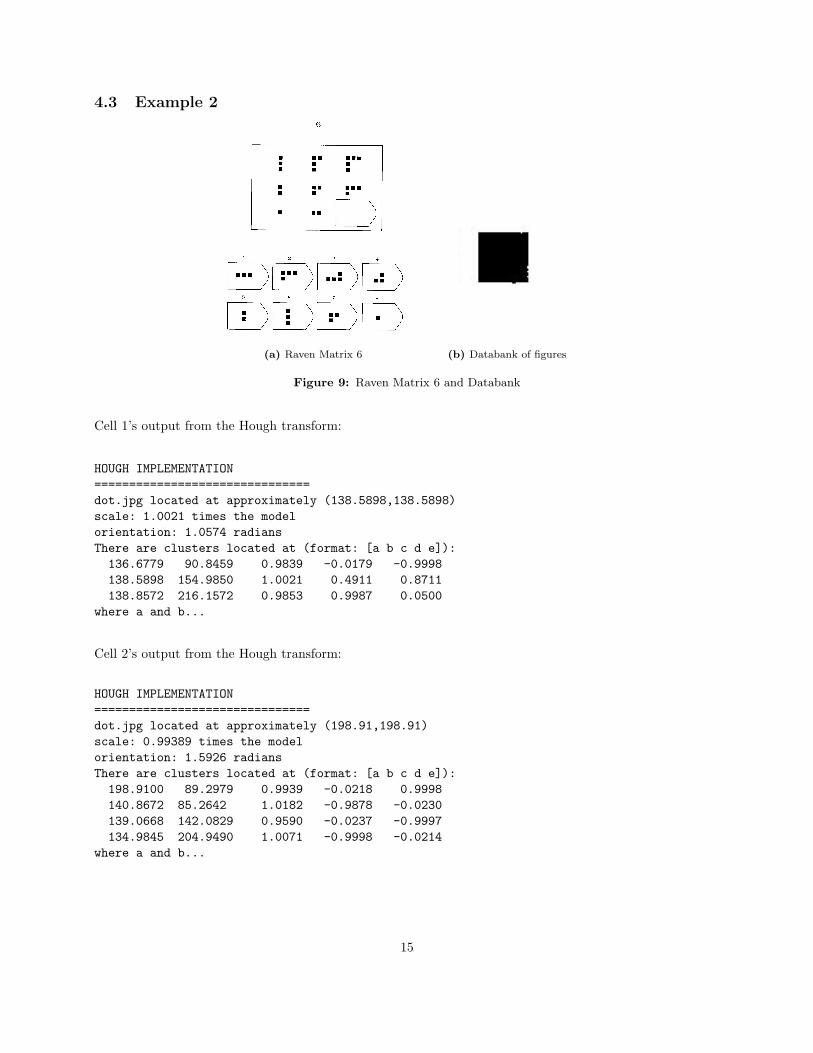
4.3 Example 2

(a) Raven Matrix 6 (b) Databank of figures

Figure 9: Raven Matrix 6 and Databank

Cell 1’s output from the Hough transform:

HOUGH IMPLEMENTATION===============================dot.jpg located at approximately (138.5898,138.5898)scale: 1.0021 times the modelorientation: 1.0574 radiansThere are clusters located at (format: [a b c d e]):136.6779 90.8459 0.9839 -0.0179 -0.9998138.5898 154.9850 1.0021 0.4911 0.8711138.8572 216.1572 0.9853 0.9987 0.0500

where a and b...

Cell 2’s output from the Hough transform:

HOUGH IMPLEMENTATION===============================dot.jpg located at approximately (198.91,198.91)scale: 0.99389 times the modelorientation: 1.5926 radiansThere are clusters located at (format: [a b c d e]):198.9100 89.2979 0.9939 -0.0218 0.9998140.8672 85.2642 1.0182 -0.9878 -0.0230139.0668 142.0829 0.9590 -0.0237 -0.9997134.9845 204.9490 1.0071 -0.9998 -0.0214

where a and b...

15

Cell 3’s output from the Hough transform:

HOUGH IMPLEMENTATION===============================dot.jpg located at approximately (102.3028,102.3028)scale: 0.99602 times the modelorientation: 0.0309 radiansThere are clusters located at (format: [a b c d e]):162.6272 72.9363 1.0117 -0.8096 0.5869216.6745 72.6565 1.0213 -0.9997 -0.0228102.1979 72.2020 1.0024 0.9995 0.032499.2356 131.1557 1.0093 -0.0115 0.999998.1655 188.9925 1.0134 0.0255 -0.9997

where a and b...

Repeat until Cell 8.

The converter would take the above output as well as the Rasmussen input for this matrix:

#horizontal dots(number);#vertical dots(number)#matrix1;32;33;31;22;23;21;12;1

#answers3; 13; 23; 22; 21; 21; 32; 21; 1

#solution3; 1

16

The converter would use the following logic:

if cell 1 contains 1 horizontal dot(s) and 3 vertical dot(s) &&cell 2 contains 2 horizontal dot(s) and 3 vertical dot(s) &&cell 3 contains 3 horizontal dot(s) and 3 vertical dot(s) &&... &&cell 8 contains 2 horizontal dot(s) and 1 vertical dot(s)

thenapply Hough transform on the answer cellsif Answer 1 contains 3 horizontal dot(s) and 1 vertical dot(s)

then output Answer 1else if Answer 2 contains 3 horizontal dot(s) and 1 vertical dot(s)

then output Answer 2...else if Answer 8 contains 3 horizontal dot(s) and 1 vertical dot(s)

then output Answer 8end

5.0 Conclusion

The problem we are trying to address is whether or not it is possible to determine the existence of a model

in a given test image. Using SIFT to determine the matching keypoints between the test and model image,

then applying the Hough transform, it is definitely possible to determine whether or not a model is found

in the test image. This method is able to determine the best possible match, in terms of the (x,y) location,

scale, and orientation, from the model to the test image. Furthermore, it is also possible to determine how

many times a particular model occurs in the image using a clustering technique.

5.1 Summary of Contributions

• demonstrated the ability to detect figures in an image using the SIFT technique and Hough transform• illustrated the ability to determine multiple occurrences of a figure in an image• developed a theoretical approach to adapt the above methods with the Rasmussen model

5.2 Future Problems

This research is just the beginning of one method to automate solving Raven’s Matrices. It is by no means

complete, and there are many things that can be improved.

17

SIFT has Limitations

Firstly, SIFT is not perfect in detecting all the keypoint matches between the test and model image. For

example, if there is a dashed line in the image that is occluded by another figure, SIFT may not be able to

detect the feature descriptors of the dashed line. Also, if the test or model image contains a lot of noise,

SIFT would also have difficulty detecting keypoints. These factors directly affect the results of the Hough

transform because it influences the number and quality of matches detected.

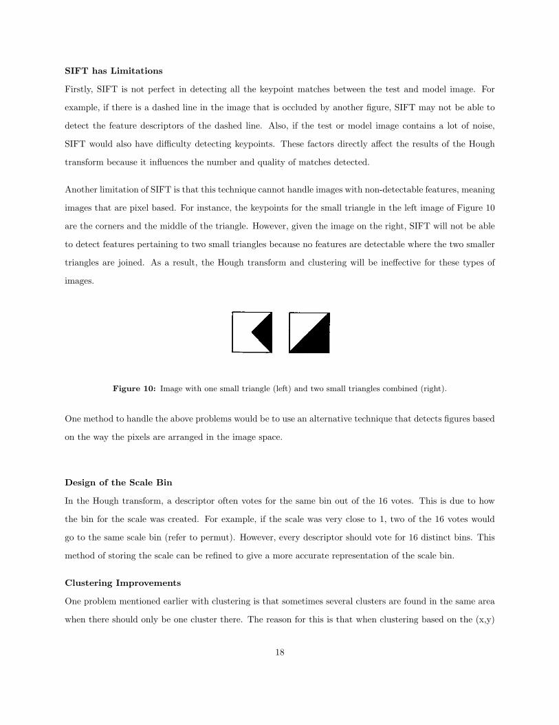
Another limitation of SIFT is that this technique cannot handle images with non-detectable features, meaning

images that are pixel based. For instance, the keypoints for the small triangle in the left image of Figure 10

are the corners and the middle of the triangle. However, given the image on the right, SIFT will not be able

to detect features pertaining to two small triangles because no features are detectable where the two smaller

triangles are joined. As a result, the Hough transform and clustering will be ineffective for these types of

images.

Figure 10: Image with one small triangle (left) and two small triangles combined (right).

One method to handle the above problems would be to use an alternative technique that detects figures based

on the way the pixels are arranged in the image space.

Design of the Scale Bin

In the Hough transform, a descriptor often votes for the same bin out of the 16 votes. This is due to how

the bin for the scale was created. For example, if the scale was very close to 1, two of the 16 votes would

go to the same scale bin (refer to permut). However, every descriptor should vote for 16 distinct bins. This

method of storing the scale can be refined to give a more accurate representation of the scale bin.

Clustering Improvements

One problem mentioned earlier with clustering is that sometimes several clusters are found in the same area

when there should only be one cluster there. The reason for this is that when clustering based on the (x,y)

18

location, scale, and orientation, the differences in orientation would indicate those data points belong to

different clusters. But since a square rotated 90 degrees is still a square, this solution would be redundant.

One way to resolve this issue would be to use a similarity transform or prior information, such as determining

that the model will not be rotated 90 degrees when mapped to the image. These methods would provide

more accurate numbers of clusters.

In this research, clustering was used only when the first bin found a match between the test and model

image. It is unknown whether or not this method provides optimal results. Further investigation into this

area would be required.

This research only adjusted the x and y radii parameters for the subclust() function. However, in the future,

all the parameters for subclust() should be compared and adjusted to find the values that provide the best

results.

Selection of Training Models

All the models in this research were taken directly from the test image. Although some models were resized

and rotated, the next step in this field of research would be to use training models that have never been

presented before. To be able to detect the presence of new figures in an image would have widespread

applications.

19

References

Ballard, D. H. (1981). Generalizing the Hough Transform to Detect Arbitrary Shapes. Pattern Recognition,

13(2), 111.

Forsyth, D. A., & Ponce, J. (2002). Fitting. Computer Vision: A Modern Approach (pp. 436)

Jirah. (2007). Raven’s Progressive Matrices. Retrieved April 3, 2010, from

http://en.wikipedia.org/wiki/Raven%27s Progressive Matrices

Lowe, D. G. (2004). Distinctive Image Features from Scale-Invariant Keypoints. International Journal of

Computer Vision, 60(2)

Raven, J. (1962). Advanced Progressive Matrices (Sets I and II). London: Lewis.

Shapiro, L., & Stockman, G. (2001). Computer Vision Prentice Hall, Inc.

Vedaldi, A. (2006). An Implementation of SIFT Detector and Descriptor. Retrieved March 29, 2010 from

http://www.vlfeat.org/∼vedaldi/code/sift.html

20

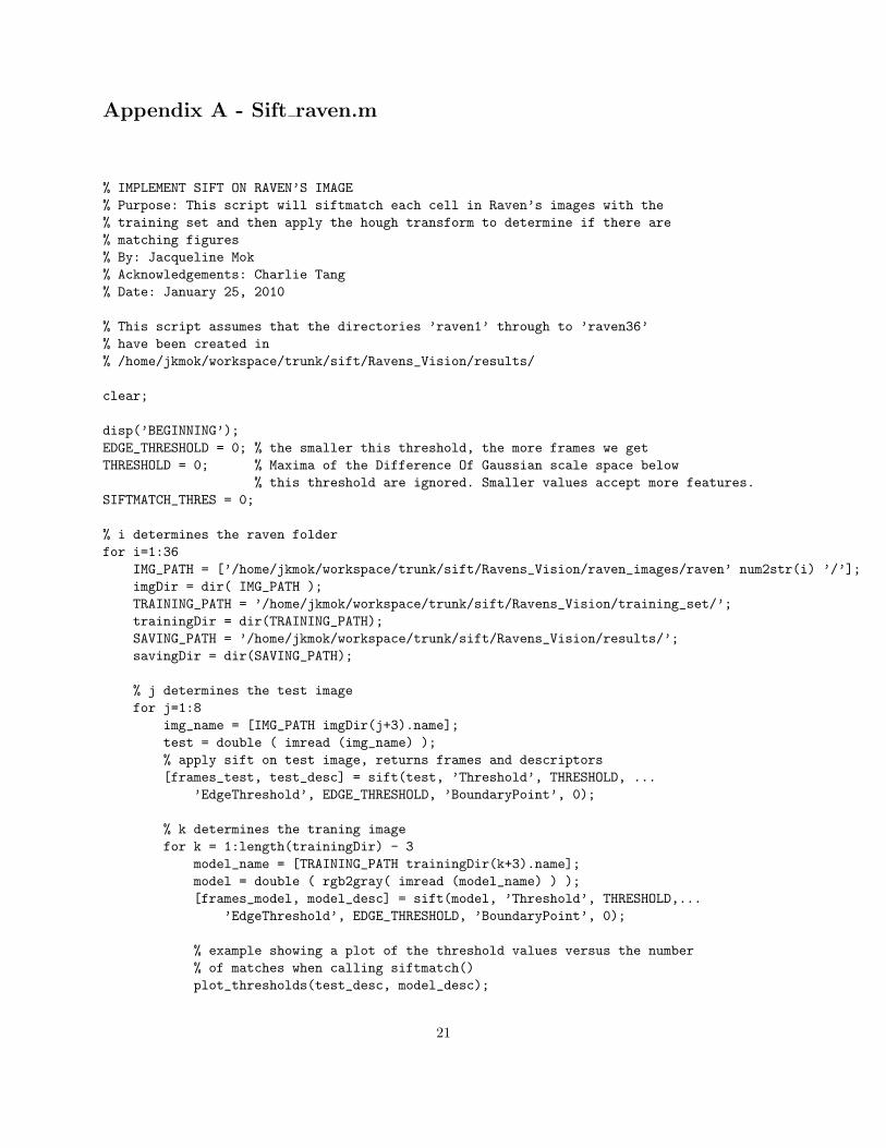
Appendix A - Sift raven.m

% IMPLEMENT SIFT ON RAVEN’S IMAGE% Purpose: This script will siftmatch each cell in Raven’s images with the% training set and then apply the hough transform to determine if there are% matching figures% By: Jacqueline Mok% Acknowledgements: Charlie Tang% Date: January 25, 2010

% This script assumes that the directories ’raven1’ through to ’raven36’% have been created in% /home/jkmok/workspace/trunk/sift/Ravens_Vision/results/

clear;

disp(’BEGINNING’);EDGE_THRESHOLD = 0; % the smaller this threshold, the more frames we getTHRESHOLD = 0; % Maxima of the Difference Of Gaussian scale space below

% this threshold are ignored. Smaller values accept more features.SIFTMATCH_THRES = 0;

% i determines the raven folderfor i=1:36

IMG_PATH = [’/home/jkmok/workspace/trunk/sift/Ravens_Vision/raven_images/raven’ num2str(i) ’/’];imgDir = dir( IMG_PATH );TRAINING_PATH = ’/home/jkmok/workspace/trunk/sift/Ravens_Vision/training_set/’;trainingDir = dir(TRAINING_PATH);SAVING_PATH = ’/home/jkmok/workspace/trunk/sift/Ravens_Vision/results/’;savingDir = dir(SAVING_PATH);

% j determines the test imagefor j=1:8

img_name = [IMG_PATH imgDir(j+3).name];test = double ( imread (img_name) );% apply sift on test image, returns frames and descriptors[frames_test, test_desc] = sift(test, ’Threshold’, THRESHOLD, ...

’EdgeThreshold’, EDGE_THRESHOLD, ’BoundaryPoint’, 0);

% k determines the traning imagefor k = 1:length(trainingDir) - 3

model_name = [TRAINING_PATH trainingDir(k+3).name];model = double ( rgb2gray( imread (model_name) ) );[frames_model, model_desc] = sift(model, ’Threshold’, THRESHOLD,...

’EdgeThreshold’, EDGE_THRESHOLD, ’BoundaryPoint’, 0);

% example showing a plot of the threshold values versus the number% of matches when calling siftmatch()plot_thresholds(test_desc, model_desc);

21

% siftmatch matches two sets of SIFT descriptorsmatches = siftmatch(test_desc, model_desc, SIFTMATCH_THRES);figure(1); clf;plotmatches(test, model, frames_test, frames_model, matches);

% apply hough transform for each test/model pairhough(matches, frames_test, frames_model, trainingDir(k+3).name, test, model);

endfprintf(’\n’);

endenddisp(’END’);

22

Appendix B - Hough.m

function [ output_args ] = hough( my_matches, frames_test, frames_model,model_name, cell, model )% this function applies the Hough transform to a set of frames from a test% and model image. If there is more than one occurrence of the model on the% test image, the a cluster function is called (cluster()). hough() takes% the following parameters:%% my_matches - the indices representing the matches between the test and% model descriptors produced by siftmatch()% frames_test, frames_model - the test and model frames containing the% (x,y) location, scale, and orientation of the descriptors% model_name - name of the model% cell, model - the test and model images

disp(’HOUGH IMPLEMENTATION’);distinct_indices=[];hashtable = java.util.Properties; % stores the bin indices

BW_x = 10; % x-bin widthBW_y = 10; % y-bin widthBW_scale = [0.05 .75 1.5 2.5 4]; % bin is the range inbetween these numbersBW_theta = 2*pi/12; %theta bin sizetest_uv = []; % used for affine fittingmodel_xy = []; % used for affine fittingbestcount = 0;winning_bin = NaN;

%figure that displays ’NO MATCH’nomatch= double(imread (’/home/jkmok/workspace/trunk/sift/Ravens_Vision/no_match.jpg’));

%for each matchfor i=1:size(my_matches, 2)

s = my_matches(1,i);t = my_matches(2,i);test_params = frames_test(:,s);model_params = frames_model(:,t);

% apply a transformation to determine where the center of the model% is mapped to on the test imagedelta_scale = test_params(3)/model_params(3);delta_theta = test_params(4) - model_params(4);

rotation = [delta_scale*cos(delta_theta) -sin(delta_theta) test_params(1); ...sin(delta_theta) delta_scale*cos(delta_theta) test_params(2); 0 0 1];

transform = rotation * [-model_params(1)+.5*size(model,2); ...-model_params(2)+.5*size(model,1); 1];

23

% determine which bin the location, scale, and orientation belong tobin_x = (transform(1) - 0.5*BW_x)/BW_x;bin_y = (transform(2) - 0.5*BW_y)/BW_y;inds = find( BW_scale > delta_scale);if size(inds, 2) == 0

bin_scale = 5;else

bin_scale = inds(1)-1;endbin_theta = (delta_theta - 0.5*BW_theta)/BW_theta;

% we want the 2 closest bins in each dimension, so we take the% floor and ceiling of the above bins. should get a total of 16params = [floor(bin_x) ceil(bin_x) floor(bin_y) ceil(bin_y) floor(bin_scale)...ceil(bin_scale) floor(bin_theta) ceil(bin_theta)];x1 = params(1); x2 = params(2); y1 = params(3); y2 = params(4);s1 = params(5); s2 = params(6); t1 = params(7); t2 = params(8);

%check for negative bins for orientation%12 is the number of bins;while t1 < 0

t1 = t1 + 12;endwhile t1 > 11

t1 = t1 - 12;endwhile t2 < 0

t2 = t2 + 12;endwhile t2 > 11

t2 = t2 - 12;end

assert(t1 >= 0); assert(t2 >= 0); assert(t1 < 2*pi/(BW_theta));assert(t2 < 2*pi/(BW_theta));% store the 16 permutations of the parameters in permutpermut = [x1 y1 s1 t1; x1 y1 s1 t2; x1 y1 s2 t1; x1 y1 s2 t2; ...x1 y2 s1 t1; x1 y2 s1 t2; x1 y2 s2 t1; x1 y2 s2 t2; ...

x2 y1 s1 t1; x2 y1 s1 t2; x2 y1 s2 t1; x2 y1 s2 t2; ...x2 y2 s1 t1; x2 y2 s1 t2; x2 y2 s2 t1; x2 y2 s2 t2];

assert(size(permut,1) == 16);

%compute hash indexfor j = 1: 16

ind = get_hash_ind( permut(j,:), 30, 4, 12);

% stores all distinct indicesif(isempty(distinct_indices(distinct_indices == ind)))

distinct_indices = [distinct_indices ind];end

24

% store indices of match is stored in the hash tableif(hashtable.containsKey(ind))

info = hashtable.get(ind);info = [info; i];hashtable.put(ind, info);

elsestore=i;hashtable.put(ind, store);

end

retrieve_info = hashtable.get(ind);current_bin_count = size(retrieve_info, 1);if current_bin_count > bestcount

bestcount = current_bin_count;winning_bin = ind;

endend

end

%==============================clustering section==========================

% X, Y, S, T store the mean (x,y) location, scale, and orientation% of the keypoints found in each bin. Tx and Ty represent the orientation% on the unit circle. allX and allY store all the (x,y) points that were% mapped to the test image. This is just used for convenience to see where% all the keypoints mapped to (plotted in figure 4).X=[];Y=[];S=[];T=[];Tx=[];Ty=[];allX=[];allY=[];firsthasmatch = 1; %assume there is a match, this is just a flag

%check if there were any matches to begin withif bestcount ~= 0

% store size of each bin in vecvec=[];for k=1:size(distinct_indices,2)

vec(k) = size(hashtable.get(distinct_indices(k)),1);end%sort descending order into sorted_bin_sizes%sorted_bin_sizes_ind stores the index of the corresponding bin in the%hash table[sorted_bin_sizes sorted_bin_sizes_ind]=sort(vec,2,’descend’);

% take the top 30 bins, used for clustering. NBin is the nth binfor NBin=1:min(size(distinct_indices,2), 30)

25

if (size(sorted_bin_sizes,1) ~= 0) && (size(sorted_bin_sizes_ind, 1) ~= 0)winning_bin = distinct_indices(sorted_bin_sizes_ind(NBin));

end

use = unique(hashtable.get(winning_bin));size_t = size(use,1);

%reset variables used for affine fittingtest_uv = [];model_xy = [];

% store all the test and model frame parametersfor i=1:size_t

testind = my_matches(1, use(i));modelind = my_matches(2, use(i));

test_uv = [test_uv frames_test(:, testind)];model_xy = [model_xy frames_model(:, modelind)];

end

model_xy = model_xy(1:2,:)’; % only take the x and y valuestest_uv = test_uv(1:2,:)’; % only take the x and y valuesaffine = zeros(size_t*2, 6);affine(int32(1:2:size_t*2),:) = [model_xy zeros(size_t, 2) repmat([1 0], size_t, 1)];affine(int32(2:2:size_t*2),:) = [zeros(size_t, 2) model_xy repmat([0 1], size_t, 1)];b = reshape(test_uv’,size_t*2,1);

m = pinv(affine)*b;

%if m does not contain any NaNif max(isnan(m)) ~= 1

%check to see where the keypoints mapped to on the test imagefirst = [m(1) m(2) m(5); m(3) m(4) m(6); 0 0 1];%the last column is for the midpoint of model%remove duplicatesmodel_xy = unique(model_xy, ’rows’);sec = model_xy’;sec = [sec [size(model,2)/2; size(model,1)/2]]; %point for the centersec(3,:) = ones(1, size(model_xy,1)+1); %row of oneschecked = first*sec;

%if there are more than 3 distinct keypoints to be mappedif( size(sec,2) - 1 >= 3)

%only plot the first bin, can change this if you want to%see all 30 binsif NBin == 1

figure(3); clf;subplot(1,2,1); imshow(cell, [0 255]); hold on;subplot(1,2,2); imshow(model, [0 255]); hold on;subplot(1,2,1); plot( checked(1,1:end-1), checked(2,1:end-1), ’ro’)

26

subplot(1,2,2); plot( sec(1,1:end-1), sec(2,1:end-1), ’ro’);subplot(1,2,1); plot( checked(1,end), checked(2,end), ’gs’)subplot(1,2,2); plot( sec(1,end), sec(2,end), ’gs’)

end

allX=[allX checked(1,1:end-1)];allY=[allY checked(2,1:end-1)];X=[X checked(1,end)];Y=[Y checked(2,end)];

tempScale=[];for a = 1:size(sec,2) - 1 %don’t want to include the midpoint

ss = norm(sec(1:2, a) - sec(1:2, end))/norm(checked(1:2, a)- checked(1:2, end));if ~isnan(ss)

tempScale=[tempScale ss];end

end

tempTheta=[];for a = 1:size(sec,2) - 1 %don’t want the midpoint that was added

tt = atan2(checked(2, a) - checked(2, end), checked(1, a) - ...checked(1, end)) - atan2(sec(2, a) - sec(2, end), sec(1, a) ...- sec(1, end));if ~isnan(tt)

while tt < 0tt = tt + 2*pi;

endtempTheta=[tempTheta tt];

endend

if(size(tempScale,1) ~= 0 && size(tempTheta,1) ~= 0)S=[S mean(tempScale)];T=[T mean(tempTheta)];

end

%display answer only for the first binif NBin == 1

disp(’===============================’);disp([model_name ’ located at approximately (’ ...

num2str(checked(1,end)) ’,’ ...num2str(checked(1,end)) ’)’]);

disp([’scale: ’ num2str(mean(tempScale)) ’ times the model’]);disp([’orientation: ’ num2str(mean(tempTheta)) ’ radians’]);

endelse

if NBin == 1disp(’===============================’);figure(3); clf;subplot(1,2,1); imshow(cell, [0 255]); hold on;

27

subplot(1,2,2); imshow(model, [0 255]); hold on;disp([’no matches for ’ model_name]);subplot(1,2,1);imshow(nomatch, [0 255]);firsthasmatch = 0;

endend

endend

if firsthasmatch ==1%now want to plot the theta values on the unit circle%take the remainder after division by 2*pi, shouldn’t have any%values over 2*pi, but do this as a safety checkT = rem(T(1,1:end), 2*pi);Tx = cos(T(1,1:end));Ty = sin(T(1,1:end));

figure(4); clf;imshow(cell, [0 255]); hold on;plot(allX, allY, ’go’)

cluster([X’ Y’ S’ Tx’ Ty’], cell);endpause(5);

elsefigure(3); clf;subplot(1,2,1); imshow(cell, [0 255]); hold on;subplot(1,2,2); imshow(model, [0 255]); hold on;disp(’no matches!’);subplot(1,2,1);imshow(nomatch, [0 255]);

endend % function

% returns serialized indexfunction [hash_ind] = get_hash_ind( vect, num_bins_y, num_bins_scale, num_bins_theta)hash_ind = vect(1)*num_bins_y*num_bins_scale*num_bins_theta + ...

vect(2)*num_bins_scale*num_bins_theta + vect(3)*num_bins_theta+vect(4);end

28

Appendix C - Cluster.m

function [ output_args ] = clust(X, cell)% this function calls Matlab’s subclust() function, which is a subtractive% clustering technique, plots a graph of the x and y radii threshold versus% the number of clusters found

%if there are unreasonably large values or if there are negative%x and y values, remove themX = X( ~any(X(:,1:2)>500, 2), :);X = X( ~any(X(:,1:2)<0, 2), :);

howmany = 100; % cap the number of times subclust is called% used to plot the x and y radii versus the number of clusters foundclust_radii = [];Xbounds = [0 0 0 -1 -1; 500 500 5 1 1];num_pixels = 0.01;incr = 10;c=1;for i=1:howmany

xy_radii = num_pixels/Xbounds(2,1);if xy_radii > 0 && xy_radii <= 1

[C S] = subclust(X, [xy_radii xy_radii 0.4 0.3 0.3], Xbounds);clust_radii=[clust_radii [xy_radii; size(C, 1)]];c = c + 1;

endnum_pixels = num_pixels + incr;

end

% plot the clusters from the last subclust() call because% this usually gives the fewest number of clusters (after% analyzing all the graphsfigure(5); clf;imshow(cell, [0 255]); hold on;plot(C(:,1), C(:,2), ’go’);% print out where the clusters are locateddisp(’There are clusters located at (format: [a b c d e]):’);disp(C);fprintf(’where a and b represent the x-y location, c represents \n...the relative scale from the model to the test image, \nand...d and e represent the angle on a unit circle. \n(cos(theta), sin(theta)) = (d,e)\n’);

figure(6);clf;hold on;plot(clust_radii(1,:), clust_radii(2,:), ’r*-’);xlabel(’x and y radii threshold’);ylabel(’number of clusters’);end

29

Appendix D - Plot thresholds.m

function [ output_args ] = plot_thresholds( test_desc, model_desc )% plot the thresholds to find out what threshold value results% in the greatest number of matches

howmany = 100;edge_thres=zeros(2, howmany);temp = 0;for m=1:howmany

matches = siftmatch(test_desc, model_desc, temp);edge_thres(1, m) = temp;edge_thres(2, m) = size(matches,2);temp = temp + 0.1;

end

figure(2); clf; hold on;plot(edge_thres(1,:), edge_thres(2,:), ’r*-’);xlabel(’siftmatch threshold’);ylabel(’number of matches’);end

30