detecting energy hot spots: experiences with the ipaq pocket pc

A P R I L 2 0 0 2

Fay Chang Keith Farkas Parthasarathy Ranganathan

Compaq Confidential

Western Research Laboratory 250 University Avenue Palo Alto, California 94301 USA

The Western Research Laboratory (WRL), located in Palo Alto, California, is part of Compaq’s Corporate Research group. WRL was founded by Digital Equipment Corporation in 1982. We focus on information tech-nology that is relevant to the technical strategy of the Corporation, and that has the potential to open new business opportunities. Research at WRL includes Internet protocol design and implementation, tools to optimize com-piled binary code files, hardware and software mechanisms to support scalable shared memory, graphics VLSI ICs, handheld computing, and more. As part of WRL tradition, we test our ideas by extensive software or hard-ware prototyping.

We publish the results of our work in a variety of journals, conferences, research reports, and technical notes. This document is a technical note. We use technical notes for rapid distribution of technical material; usually this represents research in progress. Research reports are normally accounts of completed research and may include material from earlier technical notes, conference papers, or magazine articles.

You can retrieve research reports and technical notes via the World Wide Web at:

http://www.research.compaq.com/wrl/

You can contact us about research reports and technical notes by sending e-mail to:

[email protected]

Detecting Energy Hot Spots:Experiences with the iPAQ Pocket PC

Fay Chang, Keith Farkas, and Parthasarathy Ranganathan

Palo Alto Research LaboratoriesCompaq Computer Corporation

fFay.Chang, Keith.Farkas, Parthasarathy [email protected]

1 Introduction

Energy is a critical resource for many computing systems, spurring the desire for energy-efficientsoftware. To build such software, developers need to understand the energy impact of their softwaredesign decisions. Currently, when developers reason about such decisions, they tend to rely on intu-ition. However, intuition can be misleading because most developers do not internalize an accuratemodel of the energy cost of different operations, or properly account for the relative frequency of theoperations that take place.

In this report, we describe a tool that can help developers quickly determine the energy impactof their design decisions. In particular, using our tool, a developer can quickly obtain a wealth ofinformation about the system's power and energy consumption while executing some software. Forexample, our tool can provide answers to questions like:

1. How does power consumption vary while executing the software?

2. What power states are exercised while executing the software, and how much energy is con-sumed in each of these power states?

3. Of the energy that is consumed, how much is consumed while executing each individual in-struction, procedure, and application?

Our tool is based on statistical sampling. Statistical sampling tools introduce a periodic sourceof interrupts. Whenever such an interrupt is received by the system, the tool records a sample thatcontains information about the system's state, such as a timestamp and the program counter of theinterrupted instruction. The samples gathered during a given time period can then be analyzed toproduce estimates of the system's behavior during that time period.

Previous statistical sampling tools introduce sampling interrupts that are separated by a fixedamount of time, possibly with some small variation to diminish the risk of synchronization [1, 7, 8]. Incontrast, our tool uses sampling interrupts that are separated by a fixed amount of energy consumption,which we refer to as the energy quanta. We refer to this approach as energy-driven statistical sampling(in contrast to previous time-driven statistical sampling approaches).

2

WRL TECHICAL NOTE TN-62 DETECTING ENERGY HOT SPOTS

The samples collected during energy-driven statistical sampling can be analyzed in a variety ofways. First, the average power consumed by the system during some time period is equal to theproduct of the energy quanta and the interrupt frequency during that period. Using this relationship,we can extract information about the system's power consumption. Second, the amount of energyconsumed while executing some software is estimated by the product of the energy quanta and thenumber of samples that are attributed to that software. Consequently, we can extract informationabout the system's energy consumption from the distribution of samples, i.e. the energy profile.

In this report, we illustrate the type of information that can be obtained from our tool using aprototype we built of the tool for an iPAQ handheld running PocketPC. We begin in the next section bycomparing our tool to other approaches for obtaining this information. Then,we describe our prototypeimplementation with Section 3 covering the hardware and Section 4 the software. Results are thenpresented in Section 6 for an energy-consumption study of 14 benchmarks. Finally, we summarizeour findings in Section 7, and present an analysis of the errors in our approach in Section A.

2 Other Tools

Energy-driven statistical sampling can be used to measure average power consumption and to obtaintemporal profiles or histograms of power consumption. It can also be used to measure total energyconsumption and extract energy profiles that attribute that energy consumption to the software ex-ecuted during the sampling period. While there are other tools that can provide such information, webelieve our tool offers several advantages.

First, a computer system's power usage could also be characterized using measurement equipmentlike digital meters or data acquisition systems. However, the accuracy provided by such measurementequipment would often be excessive, so that our tool is a better option owing to its much lowerhardware cost and greater ease of use.

Second, there are several other tools that seek to assist developers in mapping energy consumptionto software components. Most of these tools estimate energy consumption by multiplying activationcounts for various activities (e.g. executing a particular type of instruction) with estimates of the en-ergy consumed to perform each activity [2, 4, 9]. One advantage of this approach is that it can leverageactivation counts for background activities to more easily attribute energy consumed asynchronously.However, an activation-based approach has the disadvantage of requiring system-specific knowledgeabout what activities should be counted, and system-specific estimates of the energy consumed toperform each such activity.

An alternate approach, PowerScope [8], uses time-driven statistical sampling but adjusts for in-congruities between duration and energy consumption by including in each sample an estimate of thesystem's instantaneous power consumption. This feature allows PowerScope to weight each sampleby its instantaneous power measurement to produce, as with our tool, an energy profile. However, webelieve that our energy-driven approach is simpler to implement and while our tool and the Power-Scope approach yield similar results for current-generation systems, we believe this equality will notnecessarily hold for future-generation systems [3].

3


current-senseamplifier

monostablemultivibrator

12-bit binarycounter

Q

Energy Counter iPAQ H36xx

processor(SA 1110)

gpio

batteryterminals

BenchPower Supply

i_s

i_m

Vs

C

Vb

Vx

Figure 1: Block diagram of the iPAQ-based energy-driven sampling prototypes. The energy counteris interposed between the power supply and the iPAQ handheld computer.

3 Hardware

In this section, we describe our hardware implementation of the energy-counter and the two iPAQ-based prototype systems that use it. Both of our prototypes are based on iPAQ units that had theirFlash ROM capacity upgraded from 16 MB to 32 MB. Unit 1 is a production H3630 unit, while unit 2is a pre-production H3600 unit.

3.1 Hardware Overview

Figure 1 presents a block diagram of our two prototypes. As shown, we replaced the battery of theiPAQ handheld with a power supply, and interposed an energy counter between the power supplyand the iPAQ's electronics. We used a power supply rather than the battery to simplify our experi-mental procedure and to ensure that the iPAQ's power efficiency stays constant during experiments;Section A.1.1 discusses the consequences of using a battery. The purpose of the energy counter is togenerate an interrupt whenever a predetermined amount of energy has been consumed. The energycounter operates as follows.

As current is is drawn from the power supply by the iPAQ, a current mirror composed of a resistorand a current-sense amplifier generates a current im = � � is (the value of � is given in column 3 ofTable 1). This current im deposits charge on the positive plate of a capacitor, which acts as a currentintegrator. When the voltage across the capacitor plates reaches 2

3 of the voltage (Vx) powering themonostable multivibrator this IC generates an output pulseP , and discharges the capacitor to a voltageof Vx

3 . The capacitor then begins to accumulate charge again via im.Each pulse P indicates that the capacitor (with capacitance C Farads) has accumulated Qc Col-

oumbs, where Qc is given by Equation 1. During this time, the iPAQ will have consumed Qi =Qc

�

Coloumbs. The energy Eq consumed by the iPAQ during this time is merely the product of the chargeand the essentially constant battery-terminal voltage Vb; Equation 2 derives this equivalence.

Qc =

Z t

0im(t)dt = C �

Vx

3(1)

4


Eq =Z t

0vb(t)� is(t)dt = Qi �

Z t

0vb(t)dt = Qi � Vb (2)

We refer to Eq as the minimum energy quanta. The minimum energy quanta in our prototypes isgiven in column 4 of Table 1.

Each pulse increments the value of a 12-bit binary counter. This counter allows the user to selectthe number of minimum energy quantas that must be consumed before an interrupt is generated.Specifically, if the iPAQ's general purpose I/O line (GPIO) is connected to bit q of the counter, thenan interrupt is generated once 2(q+1) quantas of energy have been consumed. We refer to this quantityas the energy quanta. The user must select the the value of q manually.

3.2 Hardware Implementation Details

One of our design goals was to support profiling of the energy consumed by applications that use an802.11b wireless radio. To this end, we designed the energy counter so that it would measure thecurrent drawn by an iPAQ handheld and a PCMCIA sleeve. Figure 2 presents a picture of one ofthe two nearly-identical prototypes. The wiring diagram of the prototypes is shown in Figure 3(a);for ease of comparison with the block diagram of Figure 1, we have reproduced Figure 1 here asFigure 3(b).

As illustrated in Figure 3(a), we have added the current mirror to the flex that is used to conveypower to the iPAQ handheld, while the rest of the energy-counter functionality is implemented by theenergy-counter PCB. We also modified the PCMCIA sleeve so as to monitor its current consumptionand to interface the energy-counter PCB to the iPAQ handheld.

We have removed the battery from both the iPAQ handheld and the PCMCIA sleeve, and replacedeach with a piece of flex that contains a battery connector at one end, and power leads at the other(P1 and P3 in Figure 3(a)). With the iPAQ handheld, we then inserted the sense resistor R in serieswith the positive power lead (P3); Column 2 of Table 1 lists the value of the sense resistor for eachprototype. To avoid measuring the current dissipated as heat in the fuse, we located R downstream ofthe fuse. With the PCMCIA sleeve, we shorted its fuse, and connected the positive power lead (P3) to

Prototype Resistor � Minimum Energy Quanta (Eq)1, upgraded H3630 unit 100m 0.001 46�J2, upgraded pre-production H3600 unit 120m 0.0012 38�J

Table 1: Characteristics of the two prototypes. The key difference in the two prototypes is the value ofthe sense resistors used, which in turn, leads to different current-scaling factors (�) and energy quantavalues. The energy quanta was measured by running on each prototype a workload that consumeda relatively constant amount of current, and, recording this current and the period of the pulse trainthat was generated by the multivibrator. The energy quanta was then calculated as the product ofthe period, current, and the voltage at the battery terminals (4.07 V and 4.05 V respectively). Theenergy-quanta values shown in the this table are the average values obtained using three differentworkloads.

5


Figure 2: One of our two iPAQ prototypes showing the iPAQ handheld and PCMCIA sleeve, theenergy-counter PCB, and the bench supply that powers all three.

MAX 4172Rs+ Rs-V+

gnd

out

P3(+)

batteryconnector

iPAQ H3xxxbattery flex

P1(gnd)

4.1

PCMCIA sleevebattery flex

(fuse removed)

P3 (+)P1

existingfuse

int_op(gpio 24)

pcm_vdd_on(U37 pin 8)

energy counter PCB

current in

interrupt enable

R

Vddgnd

(a) Wiring diagram



12-bit binarycounter

Q


processor(SA 1110)

gpio

batteryterminals

BenchPower Supply

i_s

i_m

Vs

C

Vb

Vx

(b) Block diagram

Figure 3: The wiring diagram (a) shows the energy-counter PCB and its connection to the iPAQhandheld and associated PCMCIA sleeve. The block diagram of Figure 1 is reproduced here as Figure(b) for ease of comparison.

6


LMC 555cmos timer

V+

gnd

out

threshdischg

reset

trig gnd

V+ Q11 Q1 Q0

clr

interrupt (select one)

current in

Vddenable

5000pF(polystyrene)

1uF 10nF

10nF10

0k

100k

74VHC4040binary counter

Figure 4: The energy-counter PCB.

the downstream end of the resistor R such that the current consumed by both the sleeve and the iPAQhandheld would flow through R.

To maximize the signal to noise ratio, we installed the current mirror (MAX 4172) adjacent to thesense resistor and connected its output to the energy-counter PCB. The energy-counter PCB (shownin Figure 4) contains the monostable multivibrator and the 12-bit binary counter.

The energy-counter PCB (Figure 4) is powered by the 3.3 V source (Vdd) generated by the iPAQhandheld and distributed to the sleeve. However, since the sleeve cannot draw more than 10 mA duringsleeve initialization [5], two transistors disconnect the ICs from Vdd until a signal generated by thePCMCIA sleeve (pcm vdd on) is asserted. The 5000 pF capacitor integrates the current generated bythe current mirror and conveyed to the capacitor via the signal current in. When the pre-determinedamount of energy is consumed, the energy quanta, an interrupt request is signaled to the processorvia int op (GPIO 24). The user must manually connect this signal to one of the outputs of the binarycounter.

4 Software

In this section, we describe the software for energy-driven statistical sampling, and the simple exten-sion of this software that allows it to also support time-driven statistical sampling. The software runswithin/on the Merlin build of PocketPC for the iPAQ.

4.1 Software Overview

The software for energy-driven statistical sampling consists of on-line software for collecting sampledata, and off-line tools for processing that data. The on-line data-collection software can be dividedinto three components: (1) a set of kernel-level modifications, (2) a device driver, and (3) a programthat enables users to control data collection via a simple GUI. The kernel-level modifications include

7


modificationsOther kernel

PID RAMexecutablemappings

sample buffer64KB

Data-

Sampledata files

bufferedsample

info

Kernel device driver

programcopy

copy

Sampling

interruptISR

SamplingSampling

Enable/disable profiling collection

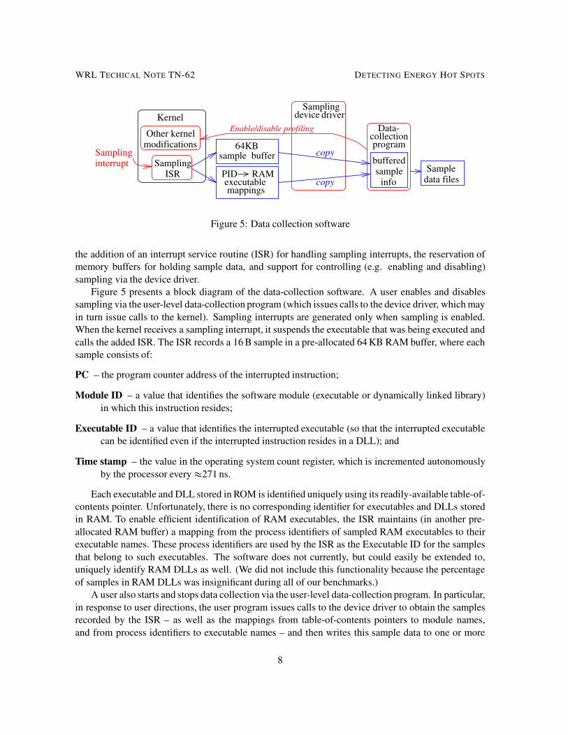
Figure 5: Data collection software

the addition of an interrupt service routine (ISR) for handling sampling interrupts, the reservation ofmemory buffers for holding sample data, and support for controlling (e.g. enabling and disabling)sampling via the device driver.

Figure 5 presents a block diagram of the data-collection software. A user enables and disablessampling via the user-level data-collection program (which issues calls to the device driver, which mayin turn issue calls to the kernel). Sampling interrupts are generated only when sampling is enabled.When the kernel receives a sampling interrupt, it suspends the executable that was being executed andcalls the added ISR. The ISR records a 16 B sample in a pre-allocated 64 KB RAM buffer, where eachsample consists of:

PC – the program counter address of the interrupted instruction;

Module ID – a value that identifies the software module (executable or dynamically linked library)in which this instruction resides;

Executable ID – a value that identifies the interrupted executable (so that the interrupted executablecan be identified even if the interrupted instruction resides in a DLL); and

Time stamp – the value in the operating system count register, which is incremented autonomouslyby the processor every �271 ns.

Each executable and DLL stored in ROM is identified uniquely using its readily-available table-of-contents pointer. Unfortunately, there is no corresponding identifier for executables and DLLs storedin RAM. To enable efficient identification of RAM executables, the ISR maintains (in another pre-allocated RAM buffer) a mapping from the process identifiers of sampled RAM executables to theirexecutable names. These process identifiers are used by the ISR as the Executable ID for the samplesthat belong to such executables. The software does not currently, but could easily be extended to,uniquely identify RAM DLLs as well. (We did not include this functionality because the percentageof samples in RAM DLLs was insignificant during all of our benchmarks.)

A user also starts and stops data collection via the user-level data-collection program. In particular,in response to user directions, the user program issues calls to the device driver to obtain the samplesrecorded by the ISR – as well as the mappings from table-of-contents pointers to module names,and from process identifiers to executable names – and then writes this sample data to one or more

8


data files. Such data files can be processed using the data-processing tools at any subsequent time toproduce various textual and graphical summaries of the sample data that was collected.

We have also extended the software to support time-driven sampling. In this mode, rather thanusing our energy counter to generate an aperiodic stream of sampling interrupts, we use one of theprocessor' s operating system timers to generate a periodic stream of sampling interrupts. Thus, ourtime-driven sampler does not require any additional hardware. The user-level data-collection programallows a user to enable either energy-driven or time-driven sampling. It also allows a user to set thesampling frequency for time-driven sampling.

4.2 Software Implementation Details

We found that attempting to write all of the sample data to the RAM-based file system while samplingis enabled noticeably disrupted the performance of the system, and therefore the samples that werecollected. Two possible approaches for addressing this problem are: 1) to decrease the amount ofdata written by writing only a subset or a summary of the sample data, and 2) to buffer the sampledata in RAM until sample collection is stopped. The first approach loses some information. Notice,however, that some of the information that can be extracted from the sample data may not be ofinterest to the particular user of the sampling system. For example, if a user of the sampling tool isinterested in energy consumption, but not in power consumption, then the time stamps in the samplesare superfluous. The amount of data saved could also be reduced by coalescing samples (e.g. byexecutable ID). In order to demonstrate the different types of information that could be extracted fromthe sample data recorded by the ISR, we currently use the second approach of buffering sample datauntil sample collection is stopped.

Table 2 summarizes the modifications and additions we made to the OEM Adaptation Layer(OAL) for the iPAQ.

5 Experimental Methodology

The experimental data we present in Section 6 was obtained using our H3630-based prototype (pro-totype #1 in Table 1); results obtained using the other prototype were similar. Using this unit, wegathered sample data with both energy-driven and time-driven sampling for the 14 benchmarks de-scribed in Table 3. While gathering this data, the iPAQ unit was not docked to a PC. Also, the PCM-CIA expansion pack was empty for all but two of the benchmarks, Idle-Conn and Download. Forthose two benchmarks, we plugged a Compaq WL100 11 Mbps Wireless LAN card into the PCMCIAexpansion pack. Before gathering any data, we changed the default system battery setting to preventthe unit from automatically powering down. We also changed the default system backlight setting toprevent the backlight from turning on (i.e. we set the brightness level to “Power Save”) for all but twoof the benchmarks, Idle-Low and Idle-Super (during which the brightness level was set to thelowest and highest on setting, respectively). We did not change any other system settings.

9


File Modificationkernel/hal/cfwzilker.c Added code to allow the sampling device driver to con-

trol whether energy/time-driven sampling is enabled ordisabled.

kernel/hal/arm/int1110.c Added interrupt service routine (ISR) that records asample upon receiving a sampling interrupt.

drivers/eprof/* New sampling device driver (which exports a stream in-terface).

drivers/dirs Added statement that causes the sampling device driverto be built by the code generation tools.

inc/drv glob.h Added global variables shared by the sampling devicedriver and the kernel.

inc/eprof.h New definitions shared by the sampling device driverand the kernel.

inc/oalintr.h Added definition of an interrupt value for sampling.files/config.bib Reserved a fixed 64 KB RAM buffer in which the

sampling ISR records samples.files/eprofgui.exe New program via which users can control sampling.

While the source for this program was not added to theOAL, it was convenient to include the executable in theiPAQ PocketPC build.

files/platform.bib Added entries so that sampling device driver and user-level program would be included in iPAQ PocketPCbuild.

files/platform.reg Added entries so that sampling device driver would beincluded as a built-in driver.

Table 2: Modifications in the OAL to implement energy-driven and time-driven statistical sampling.We also modified int1110.c, cfwzilker.c and timer.c to fix the bug in the unmodified OALcode that caused all interrupts to be cleared while servicing any interrupt (rather than clearing onlythe serviced interrupt).

Sample Collection

In our experiments, as discussed in Section 4.2, the user-level data-collection program buffered allsample data in memory until profiling was stopped in order to retain all the sample data without in-curring excessive overhead. In our energy-driven sampling experiments, we used an energy quantaof 2.94 mJ. As shown in Table 4, this quanta resulted in average sampling frequencies of between93 and 535 Hz. For our time-driven sampling experiments, we used an average sampling frequencyof 247 Hz for Record and Download and 349 Hz for all other benchmarks. As further discussedin Section A.2, this energy quanta and these sampling frequencies were small enough to ensure thatsufficient samples were collected during each of our benchmarks, but large enough to avoid notice-

10


Benchmark Description Duration (s)Idle Idle –Idle-Low Idle with brightness level set to “Low Bright” –Idle-Super Idle with brightness level set to “Super Bright” –Idle-Conn Idle with wireless card –CPU-cached Dummy CPU application that repeatedly updates a cached

integer variable34

CPU-uncached Dummy CPU application that accesses a large uncached ar-ray

40

Music Use Windows Media Player to play an MP3 file 66Music-Silent Use Windows Media Player to play the MP3 file without pro-

ducing sound65

Music-Loudest Use Windows Media Player to play the MP3 file at theloudest volume setting

65

Movie Use Windows Media Player to play a WMV file 110Record Record the MP3 file played from another machine 65Game Play Christmas Rush, a multimedia game 54Download Use Pocket Internet Explorer and wireless card to download

an uncached web page that contains many JPEG images35

CPU-cached+Game The CPU-cached benchmark followed by the Game bench-mark

84

Table 3: Benchmarks and their run time.

ably perturbing the collected sample data. For our benchmarks, they resulted in a maximum averagedata collection rate of approximately 8 KB/second, and a peak data collection rate of approximately10 KB/second. During our benchmarks, new sample data is copied into the data-collection program'suser-level buffer (and the data-collection program is awakened) at most once every 1024 samples.

6 Results

Energy-driven statistical sampling can be used to measure the average power consumption and to ob-tain temporal profiles or histograms of power consumption. It can also be used to measure total energyconsumption and extract energy profiles that attribute that energy consumption to the software ex-ecuted during the sampling period. In this section, we illustrate these uses for energy-driven samplingand the insights they provide. We also compare the results that can be obtained through energy-drivenstatistical sampling to those that can be obtained through time-driven statistical sampling, which hasthe advantage of requiring no additional hardware support.

11


Benchmark Ave sampling Ave power Number of % samplesfrequency (Hz) (mW) samples in OEMIdle

(1) (2) (3) (4)Idle 93 273 – 98Idle-Low 251 738 – 99Idle-Super 417 1226 – 99Idle-Conn 383 1126 – 99CPU-cached 260 765 8192 7CPU-uncached 381 1120 14336 14Music 230 676 16384 45Music-Silent 218 641 14216 44Music-Loudest 256 753 16384 47Movie 303 891 32768 19Record 157 462 10196 74Game 409 1202 21504 1Download 535 1573 18932 18CPU-cached+Game 348 1023 28672 3

Table 4: Average sampling frequency, corresponding average power consumption, number of samples,and percentage of samples attributed to the OEMIdle routine for each of our benchmarks. Averagepower consumption is the product of average sample frequency and the energy quanta, 2.94 mJ.

6.1 Power consumption

Energy-driven statistical sampling can be used to measure and compare the base power consumptionof the system in various modes (e.g. idle with the backlight powered at various intensities). Spe-cifically, the power consumption in some mode can be calculated as the product of the energy quantaand the average sampling frequency in that mode. Further the relative sampling frequency in twomodes indicates the relative power consumption of those modes. Table 4 presents the average powerconsumption for our benchmarks.

Column 1 of the table shows the average sampling frequency during each of our benchmarks,while column 2 provides the corresponding average power consumption. Observe that, for example,idling with the backlight on at its lowest setting (Idle-Low) causes the unit to consume 2.7 times thepower of idling with the backlight off (Idle). Alternatively, idling with the backlight off and the wire-less card inserted (Idle-Conn) causes the system to consume almost as much power as idling withthe backlight on at its highest setting without the wireless card (Idle-Super). In contrast, changingthe speaker volume at which an MP3 file is played from the lowest setting (Music-Silent) to thehighest setting (Music-Loudest) offered by Windows Media Player increased the system's powerconsumption by only 17%.

Average power consumption figures, such as those given in Column 2, do not reveal the variationin power consumption during a benchmark. However, since the energy consumed between the oc-currence of any two interrupts (samples) is constant, the average power consumed during the interval

12


between the two samples is simply the energy quanta divided by the time since the last sample. There-fore, energy-driven statistical sampling can also provide temporal profiles and histograms of powerconsumption.

6.1.1 Temporal Power-Consumption Profiles

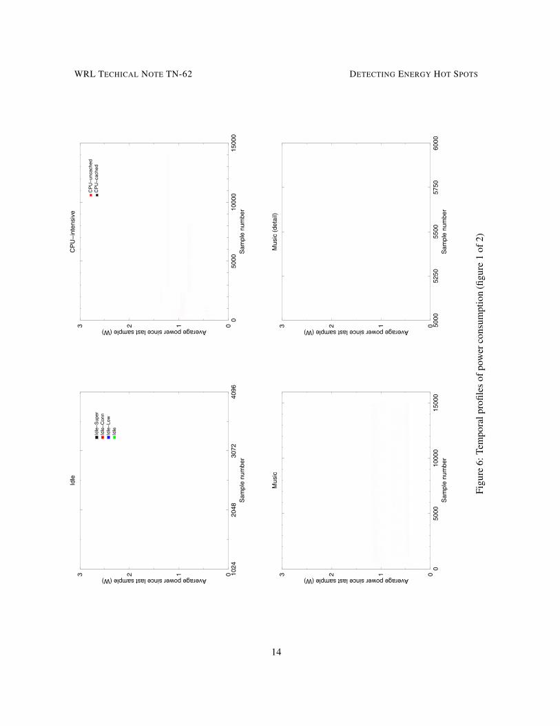
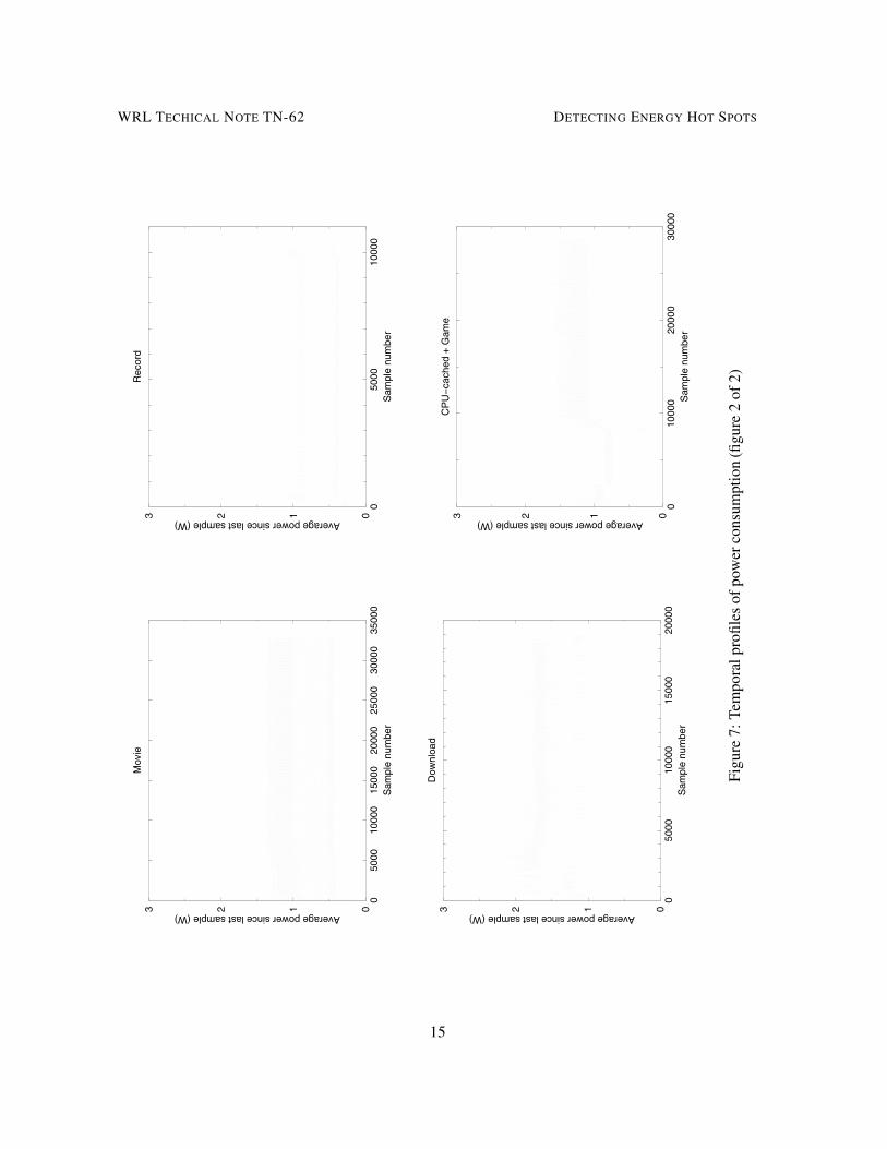
Figures 6 and 7 show temporal profiles of power consumption for a representative subset of our bench-marks. In each graph, the samples are ordered in time sequence along the x-axis, and the correspond-ing power consumption values are plotted on the y-axis. In order to show details that are obscuredwhen data points are spaced very closely, Figure 6 includes a close-up of a portion of the temporalprofile for the Music benchmark.

Spikes or shifts in temporal profiles can be correlated with events that occur during a bench-mark. For example, the noisy interval at the beginning and end of the temporal profiles of many ofthe benchmarks corresponds to touch screen navigation to start up and terminate the benchmark ap-plication, while the CPU-intensive benchmarks experience a downward shift in power consumptionwhen the audio system times out and powers itself down1. In addition, the Download benchmarkexperiences downward spikes in power consumption which correspond to times during which theiPAQ is simply waiting to receive more data, while the shift from lower to higher power consump-tion during the sequential CPU-cached + Game benchmark corresponds to the transition betweenrunning CPU-cached and running Game. The detail of the temporal profile for the Music bench-mark reveals the granularity at which the CPU alternates between idle and busy times while playingan MP3 file. During most of the benchmarks, however, sampling intervals corresponding to lowerand higher power consumption are interspersed very finely, indicating that those benchmarks do notcontain distinct phases in which they operate at different power consumption levels.

The temporal profiles also reveal that, unsurprisingly, power varies the least for the benchmarksthat contain the least amount of variation in activity (i.e. the idle and CPU-intensive benchmarks).The temporal profiles of all the other benchmarks show frequent incidence of power consumption atsubstantially different levels.

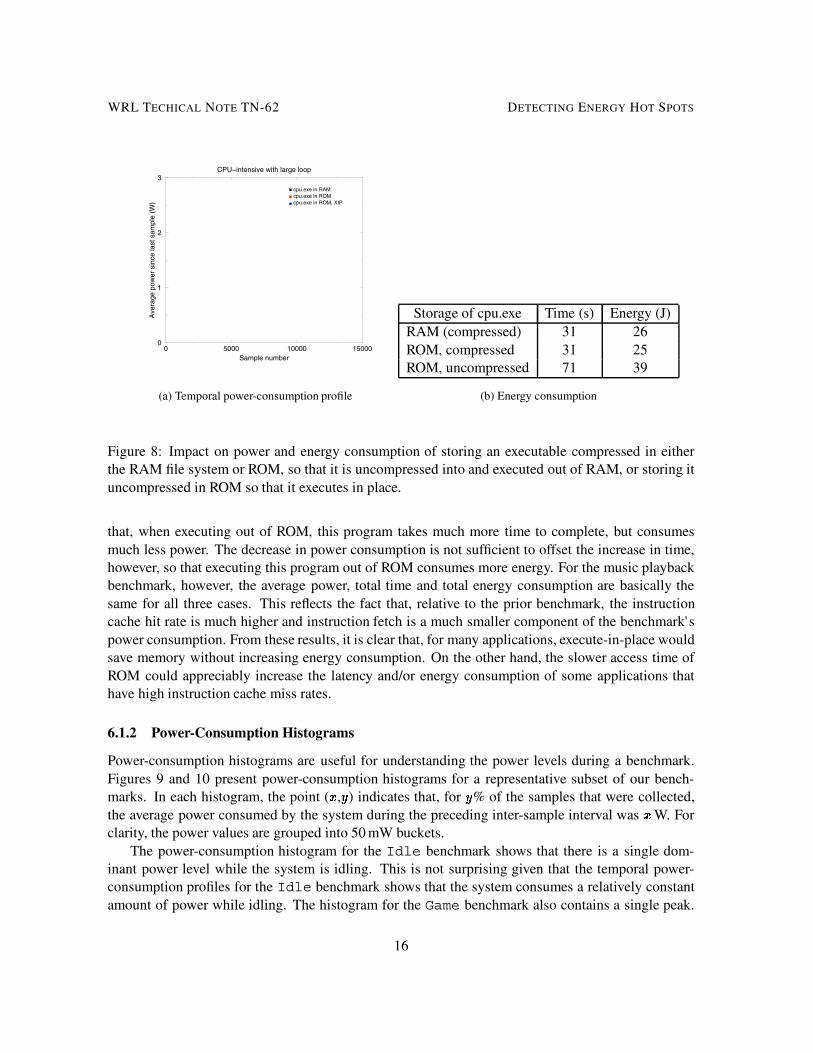
As another example of the insight that temporal profiles provide, we investigated how power andenergy consumption change depending on whether a program is stored compressed in the RAM filesystem, compressed in ROM, or uncompressed in ROM. In the first two cases, the program is uncom-pressed and paged into RAM when executed; in the latter case, the program is executed directly outof ROM. We used two benchmarks: 1) executing a contrived CPU-intensive program which consistsof a loop of simple arithmetic operations that does not fit in the processor' s instruction cache and 2)playing an MP3 file that is stored in RAM with Windows Media Player. For the execute-in-place caseof the second benchmark, we use the default compression settings in the Merlin iPAQ build, whichspecify that the resources should be compressed in ROM (and therefore decompressed and copied intoRAM before use).

For the uncacheable benchmark, Figure 8(a) shows the temporal power-consumption profiles,and Figure 8(b) shows total time and energy consumption, for all three cases. These results show

1The audio system is powered at the beginning of all the benchmarks except the idle benchmarks because the systememits some beeps during touch screen navigation to start up the benchmark applications.

13


1024

2048

3072

4096

Sam

ple

num

ber

0123 Average power since last sample (W)

Idle

Idle

−S

uper

Idle

−C

onn

Idle

−Lo

wId

le

050

0010

000

1500

0S

ampl

e nu

mbe

r


CP

U−

inte

nsiv

e

CP

U−

unca

ched

CP

U−

cach

ed

050

0010

000

1500

0S

ampl

e nu

mbe

r


Mus

ic

5000

5250

5500

5750

6000

Sam

ple

num

ber


Mus

ic (

deta

il)

Figu

re6:

Tem

pora

lpro

files

ofpo

wer

cons

umpt

ion

(figu

re1

of2)

14


050

0010

000

1500

020

000

2500

030

000

3500

0S

ampl

e nu

mbe

r


Mov

ie

050

0010

000

Sam

ple

num

ber


Rec

ord

050

0010

000

1500

020

000

Sam

ple

num

ber


Dow

nloa

d

010

000

2000

030

000

Sam

ple

num

ber


CP

U−

cach

ed +

Gam

e

Figu

re7:

Tem

pora

lpro

files

ofpo

wer

cons

umpt

ion

(figu

re2

of2)

15


0 5000 10000 15000Sample number

0

1

2

3

Ave

rage

pow

er s

ince

last

sam

ple

(W)

CPU−intensive with large loop

cpu.exe in RAMcpu.exe in ROMcpu.exe in ROM, XIP

(a) Temporal power-consumption profile

Storage of cpu.exe Time (s) Energy (J)RAM (compressed) 31 26ROM, compressed 31 25ROM, uncompressed 71 39

(b) Energy consumption

Figure 8: Impact on power and energy consumption of storing an executable compressed in eitherthe RAM file system or ROM, so that it is uncompressed into and executed out of RAM, or storing ituncompressed in ROM so that it executes in place.

that, when executing out of ROM, this program takes much more time to complete, but consumesmuch less power. The decrease in power consumption is not sufficient to offset the increase in time,however, so that executing this program out of ROM consumes more energy. For the music playbackbenchmark, however, the average power, total time and total energy consumption are basically thesame for all three cases. This reflects the fact that, relative to the prior benchmark, the instructioncache hit rate is much higher and instruction fetch is a much smaller component of the benchmark'spower consumption. From these results, it is clear that, for many applications, execute-in-place wouldsave memory without increasing energy consumption. On the other hand, the slower access time ofROM could appreciably increase the latency and/or energy consumption of some applications thathave high instruction cache miss rates.

6.1.2 Power-Consumption Histograms

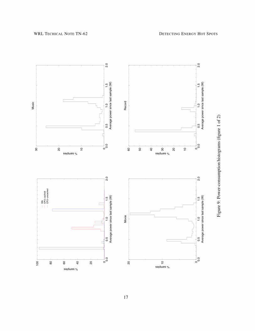
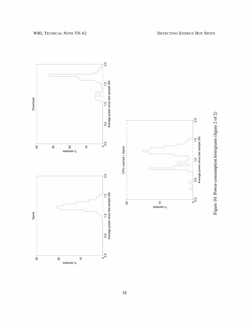
Power-consumption histograms are useful for understanding the power levels during a benchmark.Figures 9 and 10 present power-consumption histograms for a representative subset of our bench-marks. In each histogram, the point (x,y) indicates that, for y% of the samples that were collected,the average power consumed by the system during the preceding inter-sample interval was xW. Forclarity, the power values are grouped into 50 mW buckets.

The power-consumption histogram for the Idle benchmark shows that there is a single dom-inant power level while the system is idling. This is not surprising given that the temporal power-consumption profiles for the Idle benchmark shows that the system consumes a relatively constantamount of power while idling. The histogram for the Game benchmark also contains a single peak.

16


0.0

0.5

1.0

1.5

2.0

Ave

rage

pow

er s

ince

last

sam

ple

(W)

020406080100

% samples

Idle

CP

U−

cach

edC

PU

−un

cach

ed

0.0

0.5

1.0

1.5

2.0

Ave

rage

pow

er s

ince

last

sam

ple

(W)

0102030

% samples

Mus

ic

0.0

0.5

1.0

1.5

2.0

Ave

rage

pow

er s

ince

last

sam

ple

(W)

01020

% samples

Mov

ie

0.0

0.5

1.0

1.5

2.0

Ave

rage

pow

er s

ince

last

sam

ple

(W)

0102030405060

% samples

Rec

ord

Figu

re9:

Pow

er-c

onsu

mpt

ion

hist

ogra

ms

(figu

re1

of2)

17


0.0

0.5

1.0

1.5

2.0

Ave

rage

pow

er s

ince

last

sam

ple

(W)

0102030

% samples

Gam

e

0.0

0.5

1.0

1.5

2.0

Ave

rage

pow

er s

ince

last

sam

ple

(W)

010203040

% samples

Dow

nloa

d

0.0

0.5

1.0

1.5

2.0

Ave

rage

pow

er s

ince

last

sam

ple

(W)

01020

% samples

CP

U−

cach

ed +

Gam

e

Figu

re10

:Po

wer

-con

sum

ptio

nhi

stog

ram

s(fi

gure

2of

2)

18


However, the peak is wider, indicating that a range of power levels is exercised during the Gamebenchmark. Finally, the histograms for all the other benchmarks show two significant peaks, indicat-ing that there are two significant power levels during each of these benchmarks.

The main power level during the CPU-cached and CPU-uncached benchmarks correspondsto the power consumption after the audio system timed out and powered down. The higher, secondarypower level corresponds to the power consumption while the audio system was powered. The twopeaks in the power-consumption histogram for the sequential CPU-cached + Game benchmarkcorrespond to the peaks in the histograms of the individual benchmarks. Finally, to explicate thebi-modal nature of the remaining power-consumption histograms, Column 4 of Table 4 shows thepercentage of samples attributed to the OEMIdle routine for each benchmark. For each benchmark,this percentage is an estimate of the percentage of energy that was consumed while the CPU wasidling during that benchmark. Notice that the system tends to consume much less power when theCPU is idle than busy (as indicated by the power consumption figures in Column 2 of Table 4).Consequently, it is not surprising that there would be two separate peaks in the histogram of everybenchmark that consumed a substantial percentage of energy while the CPU was idling as well as asubstantial percentage of energy while the CPU was not idling. Moreover, it is not surprising thatthe lower peak should be less pronounced for the benchmarks that consumed a smaller percentage ofenergy while the CPU was idling.

Notice that the lower peak in each of the bi-modal histograms for the single-application bench-marks corresponds to a higher power level than the dominant power level during the Idle benchmark.There are several possible reasons for this difference. One hypothesis is that the periods of time dur-ing which the CPU is busy are so finely interspersed with those during which it is idle that the CPUwill have been busy for some percentage of the time between any two samples. A second hypothesisis that, when the CPU is idle, the system is not necessarily idle, and the power consumed by such“asynchronous” system activity is responsible for the increased power level.

To investigate this latter hypothesis, we modified the OAL such that we could disable the audiosystem (by powering down the speaker and audio codec, and eliminating DMA to the audio subsys-tem) and/or the LCD subsystem (by eliminating LCD refresh and DMA to the LCD subsystem). Wethen experimented with disabling these subsystem while running the multimedia benchmarks. Ourexperiments validated this hypothesis. For example, Figure 11(a) shows power-consumption histo-grams for the Music benchmark when the audio subsystem was enabled or disabled. Disabling theaudio subsystem shifted the power consumption histogram such that the lower mode is at the dominantpower level of an idle system.

From Figure 11(a) we can also gain some insight into the characteristics of this asynchronouspower consumption. In particular, note that the two peaks become more pronounced when the au-dio subsystem is disabled. This indicates that there was some variation in the asynchronous powerconsumption of the audio subsystem. This variation can obscure differences in synchronous powerconsumption. For example, Figure 11(b) shows power histograms for a game benchmark (that usesthe same game as the Game benchmark, but runs for a longer duration) when the audio and LCD sub-systems were either both enabled or both disabled. Notice that, with the audio and LCD subsystemsdisabled, the power histogram suggests a second, smaller peak at approximately 1.2 W.

Finally, leveraging this ability to power down the LCD subsystems, we found that the LCD sub-

19


0.0 0.5 1.0 1.5 2.0Average power since last sample (W)

0

10

20

30

40

% s

ampl

es

Music

Audio system poweredAudio system de−powered

0.0 0.5 1.0 1.5 2.0Average power since last sample (W)

0

10

20

30

% s

ampl

es

Game

Audio & LCD poweredAudio & LCD de−powered

Figure 11: Power-consumption histograms for the Music and Game benchmarks with various sub-systems enabled or disabled.

system consumes about 120 mW when the system is idle. In other words, LCD refresh is responsiblefor 44% of the power that is consumed when the system is idle with the backlight off and the expansionpack empty.

6.2 Energy consumption

Energy-driven statistical sampling can also be used to develop insights into energy consumption.For example, the energy consumed to perform a task can be calculated as the product of the energyquanta and the number of samples recorded while performing that task. Further, the relative numberof samples that are recorded while performing different tasks are indicative of their relative energyconsumption. Column 3 of Table 4 shows the number of samples for each of the benchmarks thatinvolved a particular task. From these figures, it can be seen that, for example, playing a particularMP3 file at the default volume consumed 1.6 times as much energy as recording that music (playedfrom a separate system) with the default microphone settings.

Energy-driven statistical sampling can also be used to extract energy profiles that apportion theenergy consumed to the software executed while the samples were collected. Specifically, since therate at which sampling interrupts occur is proportional to the rate at which energy is being consumed,the percentage of samples attributed to some software is an estimate of the percentage of energyconsumed while executing that software.

Energy profiles can be extracted at different granularities. Instruction-level profiles can be pre-pared by coalescing the samples attributed to each unique static instruction, while procedure-levelprofiles can be prepared by coalescing the samples of all instructions in a given procedure. Suchprofiles can be leveraged by application developers and system designers to direct their optimizationefforts more effectively. Module-level and executable-level profiles can be similarly obtained – the

20


latter could be leveraged by users of a system to understand how they are using up the charge storedin the battery.

Given that energy-driven statistical sampling requires a small amount of hardware support thatis not provided by most current systems, one question that warrants investigation is to what degreeduration can serve as an approximation for energy consumption. To help answer this question, the restof this section compares energy and time profiles.

6.2.1 Procedure-level Profiles

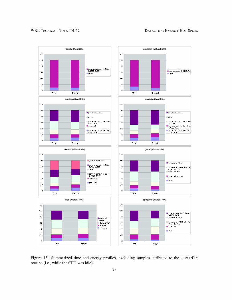
Figure 12 presents the procedure-level time and energy profiles for eight of our benchmarks. For eachbenchmark, the time and energy profiles individually identify all the procedures and modules to which10% or more of the samples were attributed within either profile. All other procedures and modulesare combined in “Other”. Procedures whose names were stripped from their binary are named asUNKNOWN <starting address> <size>. Finally, the procedures and modules in each graphare ordered according to the number of samples that time profiling attributed to that procedure/module,so that it is easy to detect when energy profiling reveals a different ordering.

Time and energy profiles differ if the profiled workload exercises multiple, distinct power levels,which, as discussed in Section 6.1.2, is true for many of our benchmarks. For example, observe that,for the benchmarks that spend a lot of time with the CPU idle, the idle routine component of thetime profile (i.e. OEMIdle) is much larger than the corresponding component of the energy profile.Similarly, the profiles for CPU-cached+Game show differences in the proportion of time and energyspent in the two executables. In particular, since time profiling is oblivious to the fact that Gameconsumes energy at a much higher rate than CPU-cached, time profiling greatly underestimates therelative energy consumption of playing the game.

If the profiled execution contains only a single dominant power level, however, time and energyprofiles will not differ substantially. This is demonstrated by the similarity of the time and energyprofiles for theGame andDownload benchmarks. It is also demonstrated by the similarity of the timeand energy profiles of all of the benchmarks except CPU-cached+Game if the samples attributed tothe OEMIdle routine are ignored, as shown in Figure 13.

6.2.2 Discussion

The similarity in most of the profiles once the OEMIdle samples are ignored is an artifact of thecurrent-generation iPAQ platform. In particular, with the exception of cache misses, all instruc-tions consume approximately the same amount of power [10]. The difference in power consump-tion due to cache misses is substantial, as illustrated by the histograms for the CPU-cached andCPU-uncached benchmarks in Figure 9. However, most procedures include a mixture of instruc-tions and, as discussed in Section 6.1.2, the power consumed by background activity represents anoteworthy fraction of the overall power consumption. As a result, the higher power consumption ofinstructions that cause cache misses is usually not sufficient to create a substantial difference betweentime and energy profiles.

Thus, the current platform exhibits only two processor-provided power states – CPU idle andCPU non-idle – that frequently result in differences between time and energy profiles. Therefore,

21


Figure 12: Summarized procedure-level time and energy profiles.

22


Figure 13: Summarized time and energy profiles, excluding samples attributed to the OEMIdleroutine (i.e., while the CPU was idle).

23


Module Time (%) Energy (%)App-206 22.01 41.13App-59 77.44 57.50Other 0.56 1.37

Module Time (%) Energy (%)App-59 31.36 20.52App-89 20.84 17.56App-118 15.67 16.32App-148 12.47 15.57App-176 10.33 14.92App-206 8.85 14.56Other 0.46 0.54

Table 5: Time and energy profiles that illustrate the impact of frequency scaling. This data wascollected using our prototype built on top of an Itsy Pocket Computer.

time-driven statistical sampling can usually be used to approximate energy-driven statistical samplingby ignoring the samples attributed to the OEMIdle routine. This conclusion, however, would not ne-cessarily apply to a system that offered the ability to dynamically and quickly change the speed at thewhich the processor runs. Such frequency changes would introduce other power states. Furthermore,future-generation processors that support voltage scaling in addition to frequency scaling are likely todisplay even greater variance in power states.

The impact that frequency and voltage scaling may have is suggested by the following two ex-periments. These two experiments were performed on a prototype we built using the Itsy PocketComputer [3]. In the first experiment, we obtained time and energy profiles for a workload consistingof running a long benchmark twice, first at a clock frequency of 206 MHz, then at a clock frequencyof 59 MHz. In the second experiment, we obtained time and energy profiles for a workload consist-ing of running a short benchmark six times, each time with a different clock frequency (206 MHz,176 MHz, 148 MHz, 118 MHz, 89 MHz and 59 MHz). Table 5 summarizes the results of these twoexperiments. While these workloads are synthetic, the results indicate the inappropriateness of timeprofiles for estimating the energy consumption of applications that exploit frequency scaling.

7 Summary and Future Work

While the issues with designing applications to reduce execution time are fairly well understood, asimilar understanding of how to design applications to reduce their energy consumption is lacking.This report presented a new approach, energy-driven statistical sampling, that exposes informationabout energy consumption. Energy-driven statistical sampling tools can help developers both reasonabout the energy impact of software design decisions and identify application energy hot spots.

Energy-driven statistical sampling uses a small amount of hardware to trigger an interrupt at pre-defined quanta of energy consumption. The interrupt is used to collect information about the programcurrently executing, and the information thus collected is processed off-line to generate an energyprofile of where energy was spent during the program's execution. Sample summaries may also begenerated that offer developers insight into the temporal power profile of the workload and the powerstates that it exercises. We have developed a prototype of this approach for the iPAQ handheld andhave presented in this report some of the insights we gathered with it. Our studies of this prototype

24


and the one we built for the Itsy pocket computer [3] indicate that energy-driven statistical samplingcan provide an accurate system-level software energy profile with very little dynamic overhead orhardware cost.

For the iPAQ prototype, we have compared energy-driven statistical sampling to time-driven stat-istical sampling by comparing the profiles generated by these approaches for 14 benchmarks pro-grams. Our results show that there are often significant differences between the profiles generatedby energy- and time-driven statistical sampling when the workload cycles through multiple powerstates. On simple handheld systems, such as current-generation iPAQ handhelds, many applicationsmay exercise only a single power state other than idle mode. In such cases, time profiling should suffi-ciently approximate energy profiling for the purpose of assisting programmers. However, preliminaryinvestigations indicate that emerging functionality, like frequency and voltage scaling, will increasethe differences between time and energy profiles, and therefore the benefit of energy-driven statisticalsampling.

A Sources of Error

In this appendix, we discuss the sources of error in our energy-driving profiling approach. Broadly,the sources of error can be classified into two categories: (i) energy measurement related, and (ii)attribution and analysis related. The rest of this section discusses each of these in detail.

A.1 Measurement-related Errors

We begin our discussion of measurement-related errors with a discussion in Section A.1.1 of an errorrelating to battery-terminal voltage variation, and follow with a discussion of other errors in Sec-tion A.1.2.

A.1.1 Battery-terminal Voltage Variations

Energy-driven profiling operates on the assumption that each interrupt signifies that the iPAQ hand-held has consumed a fixed amount of energy. Since our energy counter integrates only the currentbeing drawn by the iPAQ handheld, an equivalent assumption is that each interrupt signifies that afixed amount of charge has been consumed. For an iPAQ handheld, the degree to which this latterassumption holds depends on the degree to which the battery-terminal voltage varies.

To examine this relationship, for a range of battery-terminal voltages, we measured the currentdrawn by one of our prototypes as it ran two workloads, each of which consumed a (relatively) con-stant amount of power. Figure 14 presents the results of these experiments. Observe that there isan inverse relationship between supply current and power consumption – in particular, the currentincreases by approximately 10%, while the power consumption decreases by approximately 3%, asthe battery-terminal voltage drops from 4.2 V to 3.8 V. We hypothesize that these relationships existsbecause: (1) for a workload consuming constant power, as the battery-terminal voltage drops, thecurrent drawn must increase, and (2) as the battery-terminal voltage drops, an iPAQ handheld appearsto become more energy-efficient, and thus, the power consumption decreases.

25


70

71

72

73

74

75

76

77

3.70 3.80 3.90 4.00 4.10 4.20 4.30

battery voltage

mA

290

291

292

293

294

295

296

297

298

299

mW

current

power

(current * voltage)

(a) Backlight off

370

375

380

385

390

395

400

405

3.70 3.80 3.90 4.00 4.10 4.20 4.30

battery voltage

mA

1510

1520

1530

1540

1550

1560

1570

mW

current

power

(current * voltage)

(b) Backlight full on and WL100 802.11b card

Figure 14: Current draw and power consumption as a function of supply voltage for iPAQ prototype#2 while the iPAQ was displaying the initial PocketPC “start” screen. (a) shows the relationship withthe backlight off, while (b) shows the relationship with the backlight on at its highest setting and theWL100 802.11b card powered but with no driver loaded. Similar data was obtained with the otherprototype and other scenarios.

The dependence on battery-terminal voltage can be ignored if (1) the battery-terminal voltage isheld (essentially) constant, and (2) if the user of the profiler is interested only in comparing the relativeenergy cost of applications. If the first requirement is satisfied, then each interrupt will correspondto a fixed amount of energy. If the second requirement is true, then the user may safely ignored theexact value of the battery-terminal voltage since he/she does not need to know the value of the energyquanta. If, on the other hand, the user requires the value of the energy quanta, then an experiment,such as described in the caption of Table 1, must be done at each battery voltage of interest.

For our prototype, which uses a bench power supply, the battery-terminal voltage is sufficientlyconstant. The battery-terminal voltage is affected by two components: the regulation of the benchsupply and the voltage drop across the fuse and sense resistor (see Figure 3(a)). The second componentis the most significant since our bench supply is well-regulated. The impact of this component can beestimated by computing the relative increase in the number of samples attributed to a workload thatoccurs with decreasing battery voltage. This increase, S, is given by Equation 3, where P is the powerthe workload consumes at the nominal operating point, �P is the change in power consumption dueto a decrease in battery voltage, while I and �I are the comparable quantities for current.

S = 100�

�P ��P

P�

I +�I

I� 1

�(3)

To quantify the increase in the number of samples due to decreasing battery voltage, we determ-ined experimentally that the voltage drop across the fuse and sense resistor was at most 140 mV for aworkload with a power consumption similar to the one used for Figure 14(b). Linear interpolation ofthe data shown in this figure gives �P = 14:04mW and �I = 9:8mA, and thus, from Equation 3,

26




preloadablecount-down

counterzero


processor(SA 1110)

gpio

batteryterminals

BenchPower Supply

i_s

i_m

Vs

C

Vb

Vxnew count

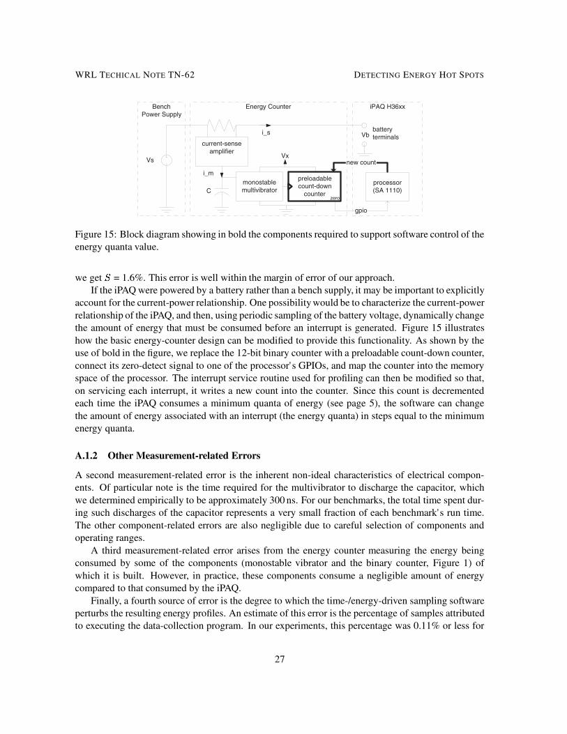
Figure 15: Block diagram showing in bold the components required to support software control of theenergy quanta value.

we get S = 1.6%. This error is well within the margin of error of our approach.If the iPAQ were powered by a battery rather than a bench supply, it may be important to explicitly

account for the current-power relationship. One possibility would be to characterize the current-powerrelationship of the iPAQ, and then, using periodic sampling of the battery voltage, dynamically changethe amount of energy that must be consumed before an interrupt is generated. Figure 15 illustrateshow the basic energy-counter design can be modified to provide this functionality. As shown by theuse of bold in the figure, we replace the 12-bit binary counter with a preloadable count-down counter,connect its zero-detect signal to one of the processor' s GPIOs, and map the counter into the memoryspace of the processor. The interrupt service routine used for profiling can then be modified so that,on servicing each interrupt, it writes a new count into the counter. Since this count is decrementedeach time the iPAQ consumes a minimum quanta of energy (see page 5), the software can changethe amount of energy associated with an interrupt (the energy quanta) in steps equal to the minimumenergy quanta.

A.1.2 Other Measurement-related Errors

A second measurement-related error is the inherent non-ideal characteristics of electrical compon-ents. Of particular note is the time required for the multivibrator to discharge the capacitor, whichwe determined empirically to be approximately 300 ns. For our benchmarks, the total time spent dur-ing such discharges of the capacitor represents a very small fraction of each benchmark's run time.The other component-related errors are also negligible due to careful selection of components andoperating ranges.

A third measurement-related error arises from the energy counter measuring the energy beingconsumed by some of the components (monostable vibrator and the binary counter, Figure 1) ofwhich it is built. However, in practice, these components consume a negligible amount of energycompared to that consumed by the iPAQ.

Finally, a fourth source of error is the degree to which the time-/energy-driven sampling softwareperturbs the resulting energy profiles. An estimate of this error is the percentage of samples attributedto executing the data-collection program. In our experiments, this percentage was 0.11% or less for

27


energy profiling, and 0.13% or less for time profiling. Although the interrupt service routine cannotbe profiled, we can measure the time spent in the routine. For time-driven sampling, the percentageof the total run time spent in the interrupt service routine is an estimate of the error it induces in theresulting time profiles. In our experiments, this percentage was 0.48% or less.

For energy-driven sampling, to estimate the error that the interrupt service routine induces in theresulting energy profiles, we first estimate the number of samples that would have been attributed tothe routine, and then express this estimate as a percentage of the total number of samples. We estimatethe number of samples that would have been attributed to the interrupt service handling routine byassuming that the average power consumption while executing the routine is approximately the sameas during the initial portion of the CPU-uncached benchmark (i.e. before the audio system waspowered down) since, as with the interrupt service routine, this benchmark is memory-intensive, doesnot include any idling, and does not use any devices. (We use the average power consumption whilethe audio system was powered because executing the interrupt service routine will not cause the audiosystem to be powered down if it is already powered.) For the Download benchmark, we adjustthe assumed power consumption of the interrupt service routine by the increase in average powerconsumption due to the wireless card (i.e. the difference between the average power consumption ofIdle and Idle-Conn). Using this process, we estimate that the percentage of samples that wouldhave been attributed to the interrupt sampling routine is 0.70% or less for all of our benchmarks. Wehave not estimated the error induced by calls to the sampling device driver because, with only theinformation currently recorded in each sample, the corresponding samples cannot be distinguishedfrom samples due to other work performed by the device manager. However, experiments on the Itsysuggest that this error will also be very small.

A.2 Attribution Error

To accurately attribute a sample to an instruction, it is important to minimize the delay between thefollowing two events: the monostable multivibrator generating a pulse P that will cause bit q of thebinary counter to be asserted (see Section 3.1), and the interruption of the program in execution sothat the interrupt can be serviced. This delay is composed of the time required for the interrupt to beconveyed to the processor core, and the time required for the processor to begin servicing the interrupt.For our prototype, the first component is on the order of nano-seconds, and is thus a small fraction ofthe time between interrupts, which is on the order of milliseconds. Given that the power consumedduring such small time intervals does not vary significantly, the first component' s impact is a marginalvariation in the energy quanta.

Regarding the second component, deferred interrupt handling could incur delay in some specificsituations (because the processor is handling a higher priority interrupt, for example), but such situ-ations occur infrequently. In addition, the iPAQ uses a StrongARM SA1110 processor. Based on ouranalysis of the SA1100 processor, which we believe uses the same core as the SA1110, one char-acteristic of this processor is that, before servicing a trap or exception, the processor first completesexecution of all instructions in the decode and later pipeline stages. Thus, when the energy-counterinterrupt is processed, the sample will be attributed to the instruction that was fetched after the instruc-tion that was in execution at the time that the interrupt was delivered to the core. Detailed informationabout instruction delays, pipeline scheduling rules and interrupt handling on the SA1110 processor

28


could be leveraged to adjust for this processor-induced skew in attribution.A second source of error arises if phases of the application being profiled are synchronized ex-

actly with the discharging of the capacitor. While we believe that this source of error is not likely tobe exercised by applications, it may be guarded against by modifying the energy counter as suggestedin Section A.1.1 to allow the value of the binary counter to be written by software. With this modi-fication, the energy quanta could be jittered by the interrupt service routine about some mean value.Our time-driven sampler trivially supports the ability to jitter its sampling frequency; in particular,during each interrupt, the time til the next sample was set to a random value within a small range suchthat the sampling frequency varied between 283 and 310 Hz during our Record and Downloadbenchmarks, and between 328 and 367 Hz during all of the other benchmarks.

Finally, a third source of error concerns sensitivity to the sampling rate. The accuracy with which asample distribution reflects the true allocation of energy consumption for an application is proportionalto the square root of the number of samples [6]. However, larger number of samples can lead to greaterprocessing overhead and increased profiler intrusiveness. We performed sensitivity experiments inwhich we lowered the energy quanta to as little as 92�J, thereby increasing the number of samples bya factor of 32. We did not observe any significant difference in the procedure-level profiles.

References

[1] J. Anderson, L. Berc, J. Dean, S. Ghemawat, M. Henzinger, S. Leung, D. Sites, M. Vandevoorde,C. Waldspurger, and W. Weihl. Continuous profiling: where have all the cycles gone. In Pro-ceedings of the 16th Symposium on Operating Systems Principles, October 1997.

[2] D. Brooks, V. Tiwari, and M. Martonosi. Wattch: A framework for architectural-level poweranalysis and optimizations. In Proceedings of the 27th International Symposium on ComputerArchitecture (ISCA), June 2000.

[3] Fay Chang, Keith I. Farkas, and Parthasarathy Ranganathan. Energy-driven statistical sampling:Detecting software hotspots. Technical Report WRL2002.1, Compaq Western Research Labor-atory, March 2002. This report is a reprint of a paper by the same title that appeared in theproceedings of the PACS 2002 workshop.

[4] T. L. Cignetti, K. Komarov, and C. Ellis. Energy estimation tools for the Palm. In Proceedingsof the ACM MSWiM'2000: Modeling, Analysis and Simulation of Wireless and Mobile Systems,August 2000.

[5] Compaq. iPAQ H3000 series expansion pack developer guide, July 2000.

[6] J. Dean, J. E. Hicks, C. Waldspurger, B. Weihl, and George Chrysos. ProfileMe: Hardwaresupport for instruction-level profiling on out-of-order processors. In Proceedings of the 30thAnnual International Symposium on Microarchitecture, December 1997.

[7] X. Zhang et al. Operating system support for automated profiling and optimization. In Proceed-ings of the 16th ACM Symposium on Operating Systems Principles, October 1997.

29


[8] J. Flinn and M. Satyanarayanan. PowerScope: A tool for profiling the energy usage of mobileapplications. In Proceedings of the Workshop on Mobile Computing Systems and Applications(WMCSA), pages 2–10, February 1999.

[9] J. Lorch and A. J. Smith. Energy consumption of Apple Macintosh computers. IEEE MicroMagazine, 18(6), November/December 1998.

[10] Amit Sinha and Anantha P. Chandrakasan. Jouletrack - a web based tool for software energyprofiling. In Design Automation Conference (DAC 2001), June 2001.

30

detecting energy hot spots: experiences with the ipaq pocket pc

Documents