detc99 dtm8766 right - drexel universityedge.cs.drexel.edu/kdi/pubs/wp99-08.pdfimpact laboratory...

IMPACT LABORATORY

IMPROVING MANUFACTURING PRODUCTIVITY WITH ADVANCED COLLABORATION TECHNOLOGY

Backward Mapping Methodology for Design Synthesis

By

Lu, S. C-Y., Bukkapatnam, S., Ge, P. and Wang, N.

Department of Aerospace and Mechanical Engineering University of Southern California

Los Angeles, CA 90089-1111

IMPACT WORKING PAPER No. WP99-08

September 1999

UNIVERSITY OF SOUTHERN CALIFORNIA

1 Copyright © 1999 by ASME

Proceedings of DETC99:1999 ASME Design Engineering Technical Conference

September 12-15, 1999, Las Vegas, Nevada

DETC99/DTM-8766

BACKWARD MAPPING METHODOLOGY FOR DESIGN SYNTHESIS

Stephen C-Y. Lu,The IMPACT Laboratory and

College of EngineeringDRB 101

University of Southern CaliforniaLos Angeles, CA 90089, U.S.A.

[email protected]

Satish TS Bukkapatnam∗

The IMPACT Laboratory andIndustrial and Systems Engineering

DRB 101University of Southern CaliforniaLos Angeles, CA 90089, U.S.A.

[email protected]

Ping GeThe IMPACT Laboratory and

Mechanical EngineeringDRB 101

University of Southern CaliforniaLos Angeles, CA 90089, U.S. A.

[email protected]

Nanxin WangFord Motor Company

P.O.Box 2053, MD 2122Dearborn, MI 48121, U.S.A.

[email protected]

∗ All the correspondences should be directed to this author.

ABSTRACT Design efficiency and robustness at early stage ofparametric engineering design play a critical role in reducingcycle time and improving product quality in the overallproduct development process. Usually, the “forward mapping”approach is used to find designs, where the desirableperformances are satisfied through large iterations of analysisand evaluation from design space to performance space.However, these approaches are time-consuming and involveblind search if the engineering system simulation modelsand/or initial conditions are not appropriately selected. On theother hand, common “reverse engineering” methods usedomain-specific assumptions and are not effective in genericscenarios where the presumed conditions are violated. In thispaper, a Backward Mapping Methodology for DesignSynthesis (BMDS) is presented that can help conduct designsynthesis rapidly and robustly at early stage of parametricengineering design. BMDS is a surrogate model-basedapproach that combines the strengths of metamodeling andstatistics. It can help designers explicitly identify the robustdesign solutions that satisfy the designer-specified performance

requirements through a “backward mapping” from theperformance space directly to the design space. Preliminarycase studies show its effectiveness and potential to be used as ageneric early stage parametric design synthesis methodology inthe future.

KEYWORDSDesign Synthesis, Backward Mapping, Metamodeling,Statistics, Early Stage of Parametric Engineering Design

INTRODUCTION Parametric engineering design happens between afunctional domain, which consists of a set of performancevariables and their ranges (or performance space), and aphysical domain, which is defined by a set of designparameters and the associated intervals (or design space). Theperformance requirements (design objectives) are defined inthe functional domain and parametric engineering design isthe process to generate feasible solution(s) in the physicaldomain to accomplish these objectives [SUH90]. Withincreased demands of frequent product model revision from


the competitive global market, most industries are using thecarry-over designs in order to expedite the time to market andreduce the cost. As a result, design, for these industries, issynonymous with the search for a new set of design parametervalues that satisfy the new requirements. Parametric design at early stage, or preliminary design,plays an important role in any product design. Research hasshown that design freedom decreases while cost increases asthe design proceeds from the early design stage to the finaldesign stage. It is at the early design stage that engineers havethe most freedom to make design changes, explore designalternatives and choose the most appropriate design(s). Aneffective early design decision provides a sound foundation forthe subsequent detailed design and all the other engineeringdecisions made later. At early stage, a large design space needsto be explored to get feasible design candidates that satisfy thegiven performance requirements for the later detailed designstages. Design analysis is commonly used to aid the search forthe acceptable design parameters. Usually, it starts with aninitial set of design parameters based on the prior designknowledge. Either physical experiments or computersimulations are performed to validate the design. If thetargeted performance requirements are met, the design isaccepted. If not, revisions to the design are made and new testsor simulations are performed until a desired solution isreached. Design optimization techniques are often used tooptimize the process. However, the emphasis at early stages should be on thederivation of a wealth of robust design alternatives as opposedto optimized isolated solutions. The computer-based simulationtools that can represent the system characteristics and mimicthe system behavior are currently used overwhelmingly togenerate, evaluate and validate designs. Since they are physics-based models, their use often requires solving a set ofnonlinear partial differential equations. For a complex designproblem these equations could become complicated and thecomputing cost is unbearable. The search for a feasible designthat satisfies the given performance requirements usuallyinvolves numerous iterations among several simulation toolsand an optimizer in current engineering practice. It isextremely time-consuming and limits engineers’ ability toevaluate more design alternatives in a given time frame. In thisscenario, an abstract model that can mimic engineering systembehavior at acceptable sacrifice of accuracy/details is moreuseful. The most popular approach is to use a surrogate modelto replace the costly model in such a situation. Usually, thesurrogate model is not as detailed nor accurate as the mostdetailed simulation model, but much more efficient to be used.Another benefit of using surrogate model is that: it has flexibleand generic representation format, which can facilitate thecommunications in multiple-stage, multiple-designerenvironments. Many metamodeling methods have beendeveloped to build surrogate models as alternatives to the

physic-based mechanistic models in order to improve designefficiency at early stage. The objective of rapid alternate robust solution renderingfor early stage design may be attained by either reducingsimulation time and/or by decreasing model iteration time.However, rapid solution rendering from the available(surrogate) models has not been addressed to date. Efficient,robust and generic methods need to be developed in order toimprove design quality at the early stage of parametricengineering design. In this paper, a Backward Mapping Methodology forDesign Synthesis (BMDS) is introduced and described. It is asurrogate model-based approach to rapidly synthesize robustdesign alternatives at early stage of parametric engineeringdesign. BMDS can help designers explicitly identify the mostrobust design regions that satisfy the designer-specifiedperformance requirements through a direct “backwardmapping” procedure from performance space to design space.In this framework, the domain knowledge of an engineeringsystem is represented in a more comprehensive and applicableform and then design synthesis is conducted based on thisrepresentation. Due to the generic form used, BMDS is capableof cross-domain utilization and the efficiency of the designprocess is improved as the result of using the fast substitute.Explicit consideration for design robustness is anotherimportant feature of BMDS. Design confidence is explicitlyaddressed and integrated with desirable performance and itsrange in the performance requirements specified by thedesigner. Unlike other methods, set-to-set mapping is used andregions instead of single points are basic design units in thisframework. The combination of metamodeling and statistics inthe framework provides a feasible way to handle modeled andunmodeled uncertainty. Compared to the “forward mapping”approaches using try-and-error iterations, BMDS avoidsineffective searches and provide the designer with explicitsense of design confidence. Compared to those in “reverseengineering” [YAMA90], it is a more generic methodologythat can be applied to many engineering domains. Itsapplication in vehicle bumper system design shows its uniquestrengths in dealing with complex, highly nonlinearengineering system design problem at early stage of parametricengineering design. In the following sections, the existing approaches arereviewed. Then BMDS and its application are described indetails. Finally, conclusions and future work are summarized.

REVIEW OF EXISTING METHODS AND THEIRLIMITATIONS There has been a lot of research effort in studying thecomplex nature of the design problems. Different designtheories and methodologies have been developed to address thedesign efficiency issue. Among them are Metamodeling andsurrogate model-based design approaches. Metamodeling has


gained more attention recently both in academia and industryapplications for they can be used to build surrogate models thatcan serve as alternatives to the physics-based mechanisticmodels. Using the surrogate models built with metamodlingtechniques can speed up performance prediction and thereforeimprove the design efficiency.

Metamodeling Metamodeling, as indicated by its name, is a technique tobuild models of models. The basic approach is to constructapproximations of the mechanistic models, which will capturethe most critical relationships between a set of designparameters: x, and a set of performance parameters: y withsome error [SIMPS97]. The existing metamodelingtechnologies include traditional statistics-based approach,kriging, machine learning-based approach and hybridapproach. The traditional statistics-based metamodeling methodslargely rely on Design of Experiment (DoE) to collect data setsfrom physical experiments and then apply regression analysisto fit a response surface [MONT97]. A response surfacerepresents a relationship between a set of independent inputvariables x and an output variable y:

y = f(x) + ε (1)

Since the true response surface function f(x) is usuallyunknown, a response surface g(x) is created to approximatef(x). Different approximation functions can be used [BOX87].These kinds of surrogate models are normally used foroptimization within Response Surface Methodology[MONT75] [MYERS89] [MYERS95]. Lately, computer simulations have been used to replace thephysical experiments for the data collection. Since thecomputer simulations are deterministic and thus not subject torandom error, the randomness assumption for the least squareregression does not hold anymore [SIMPS97]. As analternative, researchers are looking into a new modelingapproach called “Kriging”. Instead of using equation (1), thekriging approach models a response as a combination of apolynomial model and an error model:

y(x) = f(x) + Z(x) (2)

where y(x) is the unknown function of the interest, f(x) is aknown polynomial function of x, and Z(x) is an error modelrepresenting the residuals. The key element of the krigingapproach is to find Z(x) by interpolating the sampled datapoints. Different correlation functions can be used for theinterpolation process. The success of this approach depends onthe appropriate choice of the correlation functions, whichcurrently rely heavily on users’ experience and in most of the

cases, it is still a “guessing” process [SACKS89] [WELCH90][WELCH92] [KOEHL96]. Machine learning-based approaches use different type ofmetamodeling techniques. They use training data sets to learnunderlying relationships between the space of x and y, andbuild surrogate models thereon. These surrogate models maytake many forms, such as neural networks and decision trees[MONOS96] [LU90]. They have been used in manyengineering applications. In some cases, they can providemore comprehensive and accurate solutions than the statisticmethods. However, insufficient training data sets,inappropriate model validation methods or error metrics canresult in inaccurate models. A hybrid modeling approach called Adaptive andInteractive Modeling System (AIMS) [LU90] is a uniquemetamodeling tool that integrates the inductive learningalgorithms and statistics techniques with recursivedecomposition and multiple objective optimization to find thebest representation of the relationship (function) between thedesign variables and performance parameters. It has beensuccessfully applied to build metamodels for vehicle bumpersystems with success [LU98], and several large-scale, highlynonlinear engineering systems.

Surrogate model-based design theories andmethodologies Surrogate model-based design approaches use high-level,abstract model of an engineering system instead of the costlymechanistic model to conduct design. Figure 1 shows thegeneric process of surrogate model-based design procedure.

Figure 1. Surrogate Model-based Engineering Design Process

The process starts with data collection, then metamodelingtechnique is used to build the surrogate models between a setof design parameters and performance parameters, and thenthese models are used to achieve the final design solution. Thegoal is to obtain robust design results in a more efficientmanner than those approaches based on mechanistic models.The most popular surrogate model-based approaches areResponse Surface Methodology (RSM) and associated designmethodologies.

ModelingObjectives

DesignObjectives

TrainingExamples

ModelFormation

ModelUtilization

TrainingData

Surrogate Models

FinalResults

SamplingStrategies

ModelingStrategies

DesignStrategies

Experiments/Simulations


RSM is widely used for developing, improving andoptimizing product and process. RSM comprises a group ofstatistical and mathematical techniques for empirical modelbuilding and model exploitation [BOX87]. For a given designspace, different design parameter value combination (data) isselected through physical design of experiments (DoE)technique and least squares (LS) regression analysis is used tofit these data with a polynomial function, which is calledresponse surface model (refer to 1.1). Then the response modelis used as a prediction tool in the optimization to explore thedesign space seeking optimum design parameter settings[MONT75] [MYERS89] [MYERS95]. Since randomness assumption for least squares regressionanalysis is invalid for design processes that data is collected bydeterministic computer experimental design, RSM is mostlyused in physical experimental data collection- based designscenarios. Even for such situations, if the response models arenot selected adequately, the following optimization may end upblind and endless search loops. Some of the design methodologies try to combine RSMwith Genichi Taguchi’s Robust Design Principles in order toimprove design quality [ROSS88] [SIMPS97]. Unfortunately,they still can’t overcome the disadvantages that come withRSM itself mentioned above. Researchers in the “reverseengineering” use mathematical inversion to obtain designsolutions based on certain assumptions [YAMA90]. Usually,these kinds of methods depend greatly on specific domainknowledge and can’t be applied to different conditions. Newmethods need to be developed in order to get reliable designresults based on the surrogate models at the early stage ofparametric engineering design.

BACKWARD MAPPING METHODOLOGY FORDESIGN SYNTHESISOverview At early stage of parametric engineering design, the goal isto find the feasible candidate(s) that satisfies the desirableperformance requirement(s) in an initial design space. At thisstage, however, the design information is still sketchy anddesign targets are constantly changing, and therefore a singlepoint design solution that meets the performance requirementshas little relevance. The common engineering practice is tospecify targeted performance ranges and try to find set(s) ofrobust design alternatives that meets the specified performancerequirements. This is particularly important for the large-scaleengineering systems with highly nonlinear relationshipbetween its design space and performance space. Within BMDS framework, the performance requirementsare a combination of designer-specified performance range anddesign confidence level. In order to identify the effectivedesign regions, the overall design space is decomposed intofeature subregions with much more comprehensiblerepresentations of relationship between design space andperformance space. Then they are evaluated according to

certain robustness criterion and the most robust designregion(s) is selected as the result. In the following sections, thetheoretical background and overall framework of BMDS aredescribed.

THEORETICAL BACKGROUNDBasic assumptions and formulations Let the complex, highly nonlinear relationship between thedesign space and performance space be expressed by anunknown function:

y = f(x), x = [ x1, x2, … , xn]T ∈ D (3)

In which, y is a set of m performance parameters, x is a set ofn design parameters, f represents the relationship(s) betweenthem and D is a predefined design space, which consists ofvalue ranges for the above design parameters. For each singleperformance parameter (yj, j = 1, … , m), designers need tofind out the design solutions that can satisfy the requiredperformance with desirable performance range and designconfidence level. Thus, design synthesis problem is defined as:

Definition 1: For a specified performance value y0 ∈ Rm, findout the most robust design region(s) {x} ⊂ D within which anydesign solution x will yield a performance value that lieswithin a certain specified range r0 ∈ Rm of y0, with theprobability of this outcome being at least equal to a specifieddesign confidence level δ0 ∈ [0,1].

The relationship in equation (3) could be very complicatedand the m performance parameters are often coupled. Thereare usually no explicit representation can be found to modelf(x). In the BMDS framework, surrogate models are used torepresent each individual relationship between yj and x:

yj’ = fj’(x), x = [ x1, x2, … , xn]T ∈ D, j = 1, ..., m (4)

Two basic assumptions are used in BMDS:Assumption 1: The design space D in equation (4) can be

decomposed into kj sub-regions and withineach sub-region a linear function can beused to approximate fj’(x).

Thus, yj’ can be represented using a piece-wise linear function:

yj’ = ajTx + e = ∑

n

iixaj1

+ e, x ∈ Dl ⊂ D, j = 1, ..., m;

l = 1, ..., kj (5)

where, e is the error between function fj’(x) and ajTx, and Dl is

a certain subregion.Assumption 2: The error e is assumed to be identically

distributed. The piece-wise linear function(aj

Tx + e) is assumed to be a spatial


stochastic function or a random function.Within each sub-region, the errordistribution is assumed to be stationary.

A mathematical representation of Assumption 2 is:

yj’ ~ N(E(yj’), V(e)) (6)

where E(yi’) = ajTx and V(e) = σ2. This assumption holds true

only when no perceptible trend or pattern is present and maybe verified using normality plot. Therefore, the performance requirements in the Definition1can be reduced to the following equation:

{ x | P (yj’ ∈ yj0 ± rj0 | x ) ≥ δ0} , j = 1, ..., m (7)

For all the x in the effective design regions, the possibility ofall the corresponding yj’ falling into the given performancerange [yj0- rj0, yj0+ rj0] should be greater or equal to thespecified design confidence level δ0.

Overall framework As shown in Figure 2, the overall BMDS framework isrealized by five major components: Domain Re-representation;Subregion Candidacy Screening; Effective Design RegionIdentification; Missing Region Recovery; Performance Vs.Design Parameters Robustness Evaluation of DesignRegion(s).

Figure 2. Overview of the Overall Framework

Domain Re-representation is the critical part of BMDS.Based on physical domain knowledge, an engineering systemcan be characterized by a set of most important designparameters and performance parameters with the associatedvalue intervals. The complex relationship between these designparameters and performance parameters can be represented ina much more comprehensible form through metamodeling,which is called surrogate model [SIMPS97] (also refer to 1.1).AIMS is a hybrid metamodeling approach for formingempirical surrogates. Given a set of design parameters (inputs)and associated performance parameters (outputs), AIMS willbuild an empirical surrogate model to mimic the systembehavior. For a complicated engineering problem with a large-sized design space, it is very difficult to find a goodapproximation over the entire design space. AIMS thereforeuses a recursive decomposition method to split the designspace into less complicated subregions and fits each region

with an appropriate model. After AIMS operation, thecomplex, highly nonlinear relationship between design spaceand performance space is re-represented by a collection ofmore explicit and comprehensible form – piece-wise linearfunctions, which facilitates the backward mapping procedure.Detailed information and examples on how to use AIMS tobuild surrogate models can be found in [LU90] and [LU98]. Subregion Candidacy Screening is a process used to findall the qualified subregions that satisfy the targetedperformance. The linear representation in each subregion isused to calculate the upper bound (yjlmax) and lower bound(yjlmin) of performance means of this subregion (j = 1, … , m; l= 1, … , kj). For a certain given value of the performanceparameter (yj0), the subregion(s) with this value falling inbetween its performance mean range (yjlmin < yj0 < yjlmax) isselected as the Qualified subregion(s) (Dq ⊂ D, q ≤ l, l = 1, ...,kj) for further investigation. Effective Design Region Identification is conducted ineach Qualified subregion. There are two very importantparameters that decide the effective design regions. They arethe lower bound of the effective performance mean: yjqL andthe upper bound of the effective performance mean: yjqU (j = 1,… , m; q ≤ l, l = 1, ..., kj). These two parameters aredetermined by the given performance value: yj0, theperformance range: rj0, the confidence level δ0, and the qualityof the surrogate model in a qualified subregion. To find thetwo bounds, the following procedure is conducted. First, check if there exists an effective design region basedon performance distribution in each qualified subregion. Ifshaded area is larger than or equal to δ0, then there is aqualified effective design region (Figure 3).

Figure 3. EPR Qualification Check

To find the yjqL, move the performance mean distributioncurve left such that the area under the curve and within theperformance range is equal to the user-specified designconfidence level: δ = δ0 (Figure 4).

EffectiveDesign RegionIdentification

DomainRe-

representation

SubregionCandidacyScreening

FinalSpecification

RobustnessEvaluation ofDesign Region

Missing RegionRecovery

y j0+ rj0y j0 y jyj0 - rj0

Performance meandistribution densityshaded area ≥δ0


Figure 4. EPR Lower Bound

By the same token, yjqU can be obtained by moving thecurve right (Figure 5).

Figure 5. Effective Performance Range

Effective Design Region Identification becomes straightforward after we convert the original model into piece-wiselinear functions, selected all the qualified subregions andcalculated yjL and yjU. The direct inverse is used in eachqualified subregion to find the effective design region(s):

yjqL ≤ ∑n

iixaj1

≤ yjqU , x ∈ Dq ⊂ D

i =1, … , n; j=1, … , m; q ≤ l, l=1, … , kj (8)

Missing Region Recovery is performed in case theeffective performance mean bounds exceed the host subregionperformance range. The issue does not arise if δ0 > 0.5.Otherwise, we explore all design subregions iteratively startingfrom the neighbors of all qualified subregions and evaluate[yjl’L, yjl’U] ∩ [yj0 – rj0, yj0 + rj0] (j= 1, … , m; l’ ≠ q and l’ ≤ l, l =1, … , kj). If the result evaluates to null, we skip the subregion,otherwise it becomes a qualified subregion. Then effectivedesign region identification procedure as mentioned above isconducted within each recovered qualified subregion. Performance Vs. Design Parameters RobustnessEvaluation of Design Region(s) is then conducted for eacheffective design region based on the robustness criterion. Therobustness criterion represents the comprehensive sensitivity of

performance space vs. design space. Currently, two kinds ofcriteria are used: 1) effective design region hypervolume; 2)maximum(minimum-dimension of design parameters) of theeffective design region. The larger the criterion value, the lesssensitive the performance parameter to the design parameters’variations. The effective design region(s) with the largestrobustness criterion value(s) is the most robust designregion(s).(i) Effective design region hypervolume criterion: If DRj is aneffective design region in a given design space D (DRj ⊂ D),the design region volume for x ∈ DRj is defined as:

Based on the tests so far, this criterion works effectively forany type of design region. One of the difficulties is, however,for high dimension design space the calculation ofhypervolume is nontrivial.(ii) Max(Min) criterion: It refers to the use of the minimumsingle design parameter value range within a effective designregion as the robustness value for this region, and the designregion with the maximum “minimum single design parametervalue range” is the most robust design region.

Figure 6. Max(Min) Robustness Criterion

Figure 6 shows an example for a 2D (y = f(x1, x2)) designspace D. A, B, C are effective design regions identified byusing BMDS. In A, there exist two design parameter valuerange, rAx1 and rAx2. Since rAx1 < rAx2, the robustness value of Ais rAx1. Similarly, the robustness values of B and C are rBx2,rCx2. C is selected as the most robust design region since it hasthe largest robustness criterion value rCx2. This criterion isexpected to offer a simpler option for the design regions withrelatively uneven single design parameter value range. Theresearch work of its utilization conditions is currently inprogress. The above procedure can be used to realize “backwardmapping” from performance space to design space for oneperformance parameter. In a design scenario with multipleperformance parameters, the intersection of “backward

)9(...1

i

V

n

i

dx∫∫∫ ∏=

yj0 yj

Performance meandistribution density

yjqL y j0 + rj0 y j0 - rj0

δ= δ0

yjqU

y j0 yj0 - rj0

Performance meandistribution density

δ= δ0

y j0 + rj0yjqL yj

rBx1

rAx1

rAx2rBx2

rCx1

rCx2

A

B

CD

x1

x2


mapping” results for each single performance parameter isrecommended as the final result. As described above, BMDS offers a generic, efficient androbust framework to help designers make design decisions atearly stage of parametric engineering design. And bycombining a hybrid metamodeling approach with statisticalformulation and techniques, BMDS has unique advantages inhandling design synthesis problems with complex, highlynonlinear relationships.

CASE STUDIESA simple example Before applying BMDS to any real industrial designscenario, it is tested on a toy problem. A target engineeringsystem is selected. And the relationship between its designspace and performance space is assumed as the followingnonlinear function:

y = x1 + 2x2 + (2-x1) (2-x2) (10)

where x1 and x2 are design parameters and y is a performanceparameter. The design synthesis problem is described as:

In a given design space, for a desirable performance valuey0, find out the most robust design region(s) within which theperformance of any design solution will be between a certainperformance range of y0 ([y0 – r0, y0 + r0]) with a certaindesign confidence level(δ0).where the given design space is x1: [0.1, 2.1] and x2: [0.1, 2.1];the desirable performance value is Y1 = 4.5; two study cases ofdifferent performance range and design confidencecombination are selected: Case I : y0 = 4.5, r0 = 0.05, δ0 = 55% Case II: y0 = 4.5, r0 = 0.10, δ0 = 85%BMDS is applied to each case to find the most robust designregion(s) that satisfy the given performance requirements.Finally the results are validated.

Results Table 1 shows the results from the first two major steps ofBMDS. First of all, the hybrid metamodeling system AIMS isused to build more comprehensive representation for thisnonlinear system. Uniform sampling is used to pick up 21values for x1 and x2 within their range [0.1, 2.1] respectively,and the cross-product between the selected data points form thetraining data input set (21 × 21). This set is input into (10) togenerate the training data output set. The input data with theirassociated outputs together form the training data set forAIMS. After AIMS operation, the nonlinear relationshipbetween the design space and performance space (10) is re-represented by a collection of much simpler linear equationswithin 6 subregions. Among them, subregion D0, D1, D2 areidentified as the qualified subregions after “SubregionCandidacy Screening” is conducted in each single subregion.

Table 1. The Surrogate Model and Qualified subregions

Table 2 shows the results of the other three major steps ofBMDS. Within each qualified subregion, yL - yU is calculated;and it is combined with the associated subregion boundary andlinear function to form the effective design region; thenhypervolume for each effective design region is computed andused as the robustness index. The effective design region(s)with the largest robustness index value is the most robustdesign region(s). Two cases are shown in the following table.

Table 2. Design Synthesis Realization and RobustnessEvaluation

After BMDS operation, the final design results are:1) In the first case, the most robust design region that

satisfies the desirable performance between 4.45 and 4.55with 55% confidence is:

{ x | x ∈ 0.1<= x1 <=2.1 ∩ 1.1< x2 <=1.433333 ∩ 1.8860 <= 0.3x1 + 1.1x2 <= 1.9738 } (11)

yL and yU Effective DesignRegion(DRi)

D0

D1

D2

D0

D1

D2

4.476 - 4.5196

4.456 - 4.5438

4.456 - 4.5438

4.4625 - 4.5290

4.4456 - 4.5579

4.4456 - 4.5579

4.456 < = 0.60x1 + 1.1x2 + 2.24. <= 4.5438

4.456 < = 0.30x1 + 1.1x2 + 2.57. <= 4.5438

4.4456 < = 0.60x1 + 1.1x2 + 2.24. <= 4.5579

4.4456 < = 0.30x1 + 1.1x2 + 2.57. <= 4.5579

Design RegionHypervolume

4.476 <= 0.95x1 + 1.1x2 +1.855 <= 4.5197

4.4625 <= 0.95x1 +1.1x2 +1.855 <= 4.5290

0.04878

0.09689

0.06239

0.12478

0.01533

0.02333

Requiredperformancerange: rY1 = 0.05Designconfidence: δY1= 0.55

Required performance range: rY1 = 0.10Designconfidence: δY1= 0.85

Toy Design Problem

Domain Re-representation Subregion Candidacy

Screening

Ymin Ymax yes/no

subregion boundary

linear equation

D0: 0.1<= x1 <=2.1,1.766667< x2 <=2.1

D1: 0.1<= x1 <=2.1,1.433333< x2

<=1.766667

D2: 0.1<= x1 <=2.1,1.1< x2 <=1.433333

D3: 0.1<= x1 <=2.1,0.766667< x2 <=1.1

D4: 0.1<= x1 <=2.1,0.433333< x2

<=0.766667

D5: 0.1<= x1 <=2.1,0.1< x2 <=0.433333

y = 0.95x1+ 1.1x2

+ 1.855

y = 0.60x1+ 1.1x2

+ 2.24

y = 0.30x1+ 1.1x2

+ 2.57

y = -0.05x1+ 1.1x2

+ 2.955

y = -0.04x1+ 1.1x2

+ 3.34

y = -0.75x1+ 1.1x2

+ 3.725

yes

yes

no

no

no

yes

3.893 6.160

3.877 5.443

3.810 4.777

3.693 4.160

2.977 4.143

2.260 4.127

The relationship between2 design parameters (x1,x2) and a performanceparameter y in the designspace (x1[0.1, 2.1],x2[0.1, 2.1) is expressedby an original function:

y = x1+2x2+(2-x1)(2-x2)

given y = 4.5, find outthe most robust designregion(s) with a requiredperformance range anddesign confidence


2) In the second case, the most robust design region thatsatisfy the desirable performance between 4.40 and 4.60with 85% confidence is:

{ x | x ∈ 0.1<= x1 <=2.1 ∩ 1.1< x2 <=1.433333 ∩ 1.8756<= 0.3x1 + 1.1x2 <= 1.9879 } (12)

Validation of the results According to (7), the probability for the performancevalue of any design solutions within a certain effective designregion falling between the required performance range shouldbe equal to or larger than the specified design confidence. Inorder to verify that the above results satisfy this condition, atwo-step validation procedure is conducted. First of all, testingexamples (design solutions) are randomly selected in eachsubregion. Then the performances of these testing examplesare input to matlab for performance distribution analysis.1) Testing Examples Generation In each case, more than 400 design points within eacheffective subregion are randomly selected as the testingexamples.2) Performance Value Distribution Analysis The testing examples are feed into the original nonlinearrelationship simulator (10) to get the correspondingperformance values. Then these values are input to matlab forperformance distribution analysis by using normplot.

Table 3. Validation Results

In Table 3, all the values at the left hand side of “>”(including 0.544) are the normplot analysis result, which arethe probabilities of testing examples’ performances fallingbetween required performance ranges for the associatedeffective design regions, and values at the right hand side arethe given design confidence. It is necessary to point out that,since selection of testing examples affects the normplotanalysis result, this result doesn’t necessarily represent therobustness level of a certain effective design region. As shown in Table 3, all the effective design regionssatisfy condition (7) except that the result of DR0 in the firstcase is a little off. This case study shows that BMDS providesreliable design solutions that satisfy the given performancerequirements in this toy problem.

Application to vehicle bumper system design In the summer of 1997, Ford Research Laboratory initiateda project to build surrogate models for vehicle bumper system

design and analysis using AIMS. The goal was to find analternative tool for the FEA simulation models traditionallyused for bumper design and analysis. As a result, surrogatemodels are built between three key design variables and fourcritical performance parameters [LU98]. The validation withboth FEA results and test results show that the quality of thesesurrogate models are very good. The same surrogate modelsare used to test the BMDS framework.

Results Two of the surrogate models mentioned above are selectedfor the study: 1) maximum beam deflection (bxd) vs. vehicleweight (vw), beam cross-section thickness (tn) and foamdensity (fd); 2) maximum resultant rail load (rf1) vs. vehicleweight (vw), beam cross-section thickness (tn) and foamdensity (fd). The given initial design space D is: vw[3250,3452] (lbs), tn[0.75, 2.00] (mm), fd[65.0, 90.0] (g/l) [LU98]. Within BMDS framework, the Bumper System DesignSynthesis problem is described as: given the performancerequirements 1) bxd = 35 mm with required performancerange as [31, 39]mm and design confidence level as 80% and2) rf1 = 100,000N with required performance range as[96,000, 104,000]N and design confidence level as 80%, findthe most robust design region(s) that satisfy these performancerequirements. The results of each major step of BackwardMapping Methodology for Design Synthesis are shown in theTable 4, Table 5 and Table 6.

Table 4. Surrogate Models for Maximum Beam Deflection(bxd) and Qualified Subregions

In Table 4, the surrogate model for maximum beamdeflection (bxd) Vs. vehicle weight, beam cross-sectionthickness and foam density is shown under the “ Domain Re-representation”. The original design space is divided intoseven subregions and in each of them, the system isrepresented by a linear function. For each subregion, themaximum and minimum beam deflection are calculated and

x ∈ DR0P(y ∈ Y1 ± rY1 |x ) x ∈ DR1 x ∈ DR2

0.544 ≈ 0.55 0.755 > 0.55 0.632 > 0.55

0.8617 > 0.85 0.9575 > 0.85 0.8833 >0.85

Required performance range: rY1 = 0.05Design confidence:δY1= 0.55

Required performance range: rY1 = 0.10Design confidence:δY1= 0.85

Domain Re-representation Subregion Candidacy Screening

ymin ymax

yes/nosubregion oundary linear equation

D0: 3250<= vw <=3452 1.791667 < tn <=2.00 65.0<= fd <= 90.0

D1: 3250 <= vw <=3452 1.583333 < tn <= 1.791667 65.0 <= fd <= 90.0D2: 3250 <= vw <= 3452 1.375 < tn <= 1.583333 65.0 <= fd <= 90.0

D3: 3250 <= vw <= 3452 1.1666667 <= tn <= 1.375 65.0 <= fd <= 90.0D4: 3250 <= vw <= 3452 0.75 <= tn <= 1.1666667 81.666667 < fd <= 90.0

D5: 3250 <= vw <= 3452 0.75 <= tn <= 1.1666667 77.5 < fd <= 81.666667D6: 3250 <= vw <= 3452 0.75 <= tn <= 1.1666667 65.0 <= fd <= 77.5

BumperSystem

Design andAnalysis

Surrogate model:beam deflection(bxd) vs. (vw, tn, fd)

Training data:63 data points

Design space:vw:3250-3452lbstn: 0.75-2.00mmfd:65.0- 90.0 g/l

Performancerequirements:bxd = 35 mmtolerance: 4 mmconfidence: 80%

bxd = 0.007562vw + 0.01928293fd - 3.218338

bxd = 0.008532vw + 0.072024fd - 6.814529bxd = 0.015056vw + 0.164032fd - 33.91913

bxd = 0.011265vw + 0.324491fd - 28.01496bxd = -118.9631tn + 190.3157

bxd = -137.107tn + 198.708

bxd = -152.4935tn + 206.323

22.611364 24.620950

25.596374 29.120456

25.653585 32.795612

29.689733 40.077622

51.525377 101.093375

no

no

no

no

no

yes

yes

38.749788 95.877750

28.413866 91.952875


compared with the given deflection value (35 mm). Thesubregions 4 and 7 are regarded as the qualified subregions forthe next step.

Table 5. Surrogate Models for Maximum Resultant Force onRail (rf1) and Qualified Subregions

Table 5 shows the similar results for maximum resultantforce on rail (rf1) as in Table 3. The surrogate model for therf1 Vs. vehicle weight, beam cross-section thickness and foamdensity is listed under the “Domain Re-representation”. Thereare six subregions after the decomposition of the initial designspace. In each subregion, the system characteristics arerepresented by a linear form. For each subregion, themaximum and minimum resultant force on rail are calculated.After each subregion performance range is compared with thegiven rf1 value (100,000 N), subregion 2, 4 and 6 are selectedas the qualified subregions for the further utilization.

Table 6. Design Synthesis Realization and Robustness Evaluation

In Table 6, surrogate representations in the qualifiedsubregions are used to obtain the yL – yU and Effective DesignRegions for bxd and rf1 respectively. There are no missingEffective Design Regions in this case. Then Design RegionHypervolumes are calculated for each effective design regionand the one with the highest hypervolume value is the mostrobust design region that satisfies the given performancerequirements mentioned above for a certain performance. According to design region robustness evaluation, the mostrobust design region for performance bxd requirements is DR0

with the highest design region hypervolume 747.6541 and themost robust design region for performance rf1 requirements isDR1 with the highest design region hypervolume 352.5872.Therefore, the final result is the intersection of DR0 for bxdand DR1 for rf1:

{ X | X ∈ 3250 < = vw <= 3452 ∩ 65.0 <= fd <= 81.66667 ∩ 1.166667 <= tn <= 1.375 ∩

60.41496 <= 0.011265vw + 0.324491fd <= 66.21496 ∩ 4.2259 <= 2.1183tn + 0.0269fd <= 4.6659} (13)

Validation of the results In order to accurately validate the result, large data setsneed to be generated by FEA model within the final resultregion for performance distribution analysis as in toy problem.Currently, such kinds of resources are unavailable. Thus thefollowing approximate validation of the result based onavailable FEA data has been conducted:

1). Maximum Beam Deflection Vs. Thickness Validation

Figure 7. Maximum Beam Deflection Vs. Thickness Validation

Given performance requirements (bxd = 35 mm, requiredperformance range = 4 mm, design confidence = 80%), theassociated design region (performance 31 mm ∼ 39 mm) fromFEA result is 1.195 < tn < 1.370.

yL - yU Effective Design Region (DRi)

D3

D1

D3

Design Region Hypervolume

bxd

rf1

32.40 - 38.20

33.55 - 38.15

97,000 - 102,437.5

98,050 - 102,450

96,900 - 103,000

DR0: 3250 <= vw <= 3452 ∩ 65.0 <= fd <= 90.0 ∩ 1.166667 <= tn <= 1.375 ∩ 60.41496 <= 0.011265vw + 0.324491fd <= 66.21496

DR1: 3250 <= vw <= 3452 ∩ 65.0 <= fd <= 77.5 ∩ 1.1028 <= tn <= 1.1330

76.255

DR2: 3250 <= vw <= 3452 ∩ 65.0 <= fd <= 73.33333 ∩ 1.1279 <= tn <= 1.166667

DR0: 3250 <= vw <= 3452 ∩ 81.66667 <= fd <= 90.0 ∩ 1.1823 <= tn <= 1.2475

65.257

109.753

DR1: 3250 <= vw <= 3452 ∩ 65.0 <= fd <= 81.66667 ∩1.166667 <= tn <= 1.583333 ∩ 4.2259 <= 2.1183tn + 0.0269fd <= 4.6659

747.654

352.587

D6

D5

3.007.00

11.0015.0019.0023.0027.0031.0035.0039.0043.0047.0051.0055.0059.0063.0067.0071.0075.0079.0083.0087.0091.00

0.75 0.85 0.93 1.00 1.10 1.12 1.14 1.25 1.27 1.40 1.50 1.55 1.60 1.75 2.00

Thickness mm

Beam

Def

lect

ion

mm

FEA

AIMS

CBUMP

Domain Re-representation Subregion CandidacyScreening

ymin ymax yes/nosubregion boundary linear equation

D1: 3250 <= vw <= 3452 0.75 <= tn <= 1.375 81.666667 < fd <= 90.0

D2: 3250 <= vw <= 34521.583333 <tn <= 2.00 65.0 <= fd <= 81.666667

D3: 3250<= vw <= 34521.166667 < tn <= 1.583333 65.0 <= fd <= 81.666667

D4: 3250 <= vw <= 34520.75 <= tn <=1.16666773.333333< fd <= 81.666667

D5: 3250 <= vw <= 34520.75 <= tn <= 1.16666765.0 <= fd <= 73.333333

BumperSystem

Design and Analysis

D0: 3250 <= vw <= 3452 1.375 < tn <= 2.00 81.666667 < fd <= 90.0Surrogate model:

resultant force on rail (rf1)vs. (vw, tn, fd)

Training data:63 data points

Design space:vw: 3250 - 3452 lbstn: 0.75 - 2.00 mmfd: 65.0 - 90.0 g/l

Performance requirements:rf1 = 100,000Ntolerance: 4,000 Nconfidence: 80%

rf1 = 12502.86tn+ 98120.70

rf1 = 83399.66tn - 1603.14

rf1 = 18.75825vw+ 5182.5tn + 300.0251fd + 15811.89

rf1 = 21182.61tn+268.9724fd+ 55791.21

rf1 = 98137.1tn - 17346.42

rf1 = 111273.7tn- 28607.47

115312.1325 123126.4200 no

no

no

60946.6050 113071.3925

104483.4573 115432.4200

97987.4680 111296.4150

56256.4050 97146.8960

54847.8050 101211.8838

yes

yes

yes


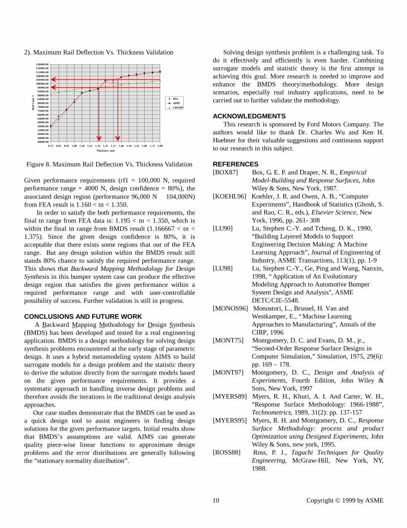
2). Maximum Rail Deflection Vs. Thickness Validation

Figure 8. Maximum Rail Deflection Vs. Thickness Validation

Given performance requirements (rf1 = 100,000 N, requiredperformance range = 4000 N, design confidence = 80%), theassociated design region (performance 96,000 N ∼ 104,000N)from FEA result is 1.160 < tn < 1.350. In order to satisfy the both performance requirements, thefinal tn range from FEA data is: 1.195 < tn < 1.350, which iswithin the final tn range from BMDS result (1.166667 < tn <1.375). Since the given design confidence is 80%, it isacceptable that there exists some regions that out of the FEArange. But any design solution within the BMDS result stillstands 80% chance to satisfy the required performance range.This shows that Backward Mapping Methodology for DesignSynthesis in this bumper system case can produce the effectivedesign region that satisfies the given performance within arequired performance range and with user-controllablepossibility of success. Further validation is still in progress.

CONCLUSIONS AND FUTURE WORK A Backward Mapping Methodology for Design Synthesis(BMDS) has been developed and tested for a real engineeringapplication. BMDS is a design methodology for solving designsynthesis problems encountered at the early stage of parametricdesign. It uses a hybrid metamodeling system AIMS to buildsurrogate models for a design problem and the statistic theoryto derive the solution directly from the surrogate models basedon the given performance requirements. It provides asystematic approach in handling inverse design problems andtherefore avoids the iterations in the traditional design analysisapproaches. Our case studies demonstrate that the BMDS can be used asa quick design tool to assist engineers in finding designsolutions for the given performance targets. Initial results showthat BMDS’s assumptions are valid. AIMS can generatequality piece-wise linear functions to approximate designproblems and the error distributions are generally followingthe “stationary normality distribution”.

Solving design synthesis problem is a challenging task. Todo it effectively and efficiently is even harder. Combiningsurrogate models and statistic theory is the first attempt inachieving this goal. More research is needed to improve andenhance the BMDS theory/methodology. More designscenarios, especially real industry applications, need to becarried out to further validate the methodology.

ACKNOWLEDGMENTS This research is sponsored by Ford Motors Company. Theauthors would like to thank Dr. Charles Wu and Ken H.Huebner for their valuable suggestions and continuous supportto our research in this subject.

REFERENCES[BOX87] Box, G. E. P. and Draper, N. R., Empirical

Model-Building and Response Surfaces, JohnWiley & Sons, New York, 1987.

[KOEHL96] Koehler, J. R. and Owen, A. B., “ComputerExperiments”, Handbook of Statistics (Ghosh, S.and Rao, C. R., eds.), Elsevier Science, NewYork, 1996, pp. 261- 308

[LU90] Lu, Stephen C.-Y. and Tcheng, D. K., 1990,“Building Layered Models to SupportEngineering Decision Making: A MachineLearning Approach”, Journal of Engineering ofIndustry, ASME Transactions, 113(1), pp. 1-9

[LU98] Lu, Stephen C.-Y., Ge, Ping and Wang, Nanxin,1998, “Application of An EvolutionaryModeling Approach to Automotive BumperSystem Design and Analysis", ASMEDETC/CIE-5548.

[MONOS96] Monostori, L., Brussel, H. Van andWestkamper, E., “Machine LearningApproaches to Manufacturing”, Annals of theCIRP, 1996

[MONT75] Montgomery, D. C. and Evans, D. M., jr.,“Second-Order Response Surface Designs inComputer Simulation,” Simulation, 1975, 29(6):pp. 169 – 178.

[MONT97] Montgomery, D. C., Design and Analysis ofExperiments, Fourth Edition, John Wiley &Sons, New York, 1997

[MYERS89] Myers, R. H., Khuri, A. I. And Carter, W. H.,“Response Surface Methodology: 1966-1988”,Technometrics, 1989, 31(2): pp. 137-157

[MYERS95] Myers, R. H. and Montgomery, D. C., ResponseSurface Methodology: process and productOptimization using Designed Experiments, JohnWiley & Sons, new york, 1995.

[ROSS88] Ross, P. J., Taguchi Techniques for QualityEngineering, McGraw-Hill, New York, NY,1988.

40000.0044000.0048000.0052000.0056000.0060000.0064000.0068000.0072000.0076000.0080000.0084000.0088000.0092000.0096000.00

100000.00104000.00108000.00112000.00116000.00120000.00

0.75 0.85 0.93 1.00 1.10 1.12 1.14 1.25 1.27 1.40 1.50 1.55 1.60 1.75 2.00

Thickness mm

Rai

l Loa

d N

FEA

AIMS

CBUMP


[SACKS89] Sacks, J., Welch, W. J., Mitchell, T. J. andWynn, H. P., “Design and Analysis of ComputerExperiments”, Statistical Science, 1989, 4(4):pp. 409-435

[SIMPS97] Simpson, Timothy W., Peplinski, J., Koch,Patrick N. and Allen, Janet K., “On the Use ofStatistics In Design and the Implications forDeterministic Computer Experiments”,Proceedings of 1997 ASME Design EngineeringTechnical Conferences (DETC’97), September14-17, 1997, Sacramento, California,DETC97/DTM3881.

[SUH90] Suh, Nam P., The Principles of Design,OXFORD UNIVERSITY PRESS, New YorkOxford, 1990

[WELCH90] Welch, W. J., Yu, T.-K., Kang, S. M. andSacks, J., “Computer Experiments for QualityControl by Parameter Design”, Journal ofQuality Technology, 1990, 22(1): pp. 15-22

[WELCH92] Welch, W. J., Buck, R. J., Sacks, J., Wynn, H.P., Mitchell, T. J. and Morris, M. D., “Screening, Predicting, and ComputerExperiments”, Technometrics, 1992, 34(1): pp.15 –25

[YAMA90] Yamaguti, M., Hayakawa, K., Iso, Y. and Mori.M.,etc., 1990, Inverse Problem in EngineeringScience, Springer-Verlag, London.

detc99 dtm8766 right - drexel universityedge.cs.drexel.edu/kdi/pubs/wp99-08.pdfimpact laboratory...

Documents