designing the logistics network - ieu.edu.trhomes.ieu.edu.tr/~aornek/wiley - introduction to...

3

Designing the Logistics Network

3.1 Introduction

In business logistics the network planning process consists of designing the systemthrough which commodities flow from suppliers to demand points, while in the publicsector it consists of determining the set of facilities from which users are serviced. Inboth cases the main issues are to determine the number, location, equipment and sizeof new facilities, as well as the divestment, displacement or downsizing of facilities.Of course, the objectives and constraints vary depending on the sector (private or pub-lic) and on the type of facilities (plants, CDCs, RDCs, regional and field warehouses,retail outlets, dumpsites, incinerators, ambulance parking places, fire stations, etc.).The aim generally pursued in business logistics is the minimization of the annualtotal logistics cost subject to side constraints related to facility capacity and requiredcustomer service level (recall the discussion in Chapter 1). As a rule, the cost tobe minimized is associated with facility operations (manufacturing, storage, sorting,consolidation, selling, incineration, parking, etc.), and to transportation between facil-ities, or between facilities and users. Also, when designing the logistics network fora utility company, different objectives, such as achieving equity in servicing users,may have to be considered.

Research in logistics network design dates back to the early location theories ofthe 19th century. Since then a variety of models and solution methodologies has beenproposed and analysed. In this chapter some of the most important facility locationproblems are examined. To put this analysis in the right perspective, a number ofrelevant issues are first introduced and discussed.

When location decisions are needed. Facility location decisions must obviouslybe made when a logistics system is started from scratch. They are also required as aconsequence of variations in the demand pattern or spatial distribution, or followingmodifications of materials, energy or labour cost. In particular, location decisions areoften made when new products or services are launched, or outdated products arewithdrawn from the market.

Introduction to Logistics Systems Planning and Control G. Ghiani, G. Laporte and R. Musmanno© 2004 John Wiley & Sons, Ltd ISBN: 0-470-84916-9 (HB) 0-470-84917-7 (PB)

TLFeBOOK

74 DESIGNING THE LOGISTICS NETWORK

Location decisions may be strategic or tactical. Whereas facilities are purchasedor built, location decisions involve sizeable investments. In this case, changing sites orequipment is unlikely in the short or medium term. This may be true even if facilitiesare leased. On the other hand, if space and equipment are rented (e.g. from a publicwarehouses) or operations are subcontracted, location decisions can be reversible inthe medium term.

Location and allocation decisions are intertwined. Location decisions are strictlyrelated to those of defining facility area boundaries (i.e. allocating demand to facili-ties). For example, in a two-echelon distribution system (see Figure 3.1), opening anew RDC must be accompanied by a redefinition of the sales districts along with a dif-ferent allocation of the RDCs to the CDCs and of the CDCs to the production plants.For this reason location problems are sometimes referred to as location–allocationproblems.

Location decisions may affect demand. Facility location may affect the demandvolume. For example, opening a new RDC may lead to the acquisition of customerswho previously could not be served at a satisfactory level of service because theylived too far away.

3.2 Classification of Location Problems

Location problems come in a variety of forms, which can be classified with respectto a number of criteria. The classification proposed below is logistics-oriented.

Time horizon. In single-period problems, facility location decisions must be madeat the beginning of the planning horizon on the basis of the forecasted logistics require-ments. In multi-period problems one has to decide, at the beginning of the planninghorizon, a sequence of changes to be made at given time instants within the planninghorizon.

Facility typology. In single-type location problems, a single type of facility (e.g.only RDCs) are located. Instead, in multi-type problems several kinds of facility (e.g.both CDCs and RDCs) are located.

Material flows. In single-commodity problems it can be assumed that a single homo-geneous flow of materials exists in the logistics system, while in multicommodityproblems there are several items, each with different characteristics. In the latter caseeach commodity is associated with a specific flow pattern.

Interaction among facilities. In complex logistics systems there can be materialflows among facilities of the same kind (e.g. component flows among plants). In thiscase, optimal facility locations depend not only on the spatial distribution of finished

TLFeBOOK

DESIGNING THE LOGISTICS NETWORK 75

Supply points

Production plants

RDCs

Figure 3.1 A two-echelon single-type location problem.

product demand but also on the mutual position of the facilities (location problemswith interaction).

Dominant material flows. Single-echelon location problems are single-type prob-lems such that either the material flow coming out or the material flow entering thefacilities to be located is negligible. In multiple-echelon problems, both inbound andoutbound commodities are relevant. This is the case, for example, when DCs have tobe located taking into account both the transportation cost from plants to DCs and thetransportation cost from DCs to customers. In multiple-echelon problems, constraintsaiming at balancing inbound and outbound flows have to be considered.

Demand divisibility. In some distribution systems it is required, for administrativeor book-keeping reasons, that each facility or customer be supplied by a single centre,while in others a facility or a customer may be served by two or more centres. In theformer case demand is said to be divisible while in the latter it is indivisible.

Influence of transportation on location decisions. Most location models assumethat transportation cost between two facilities, or between a facility and an user, iscomputed as a suitable transportation rate multiplied by the freight volume and thedistance between the two points. Such an approach is appropriate if vehicles travel bymeans of a direct route. However, if each vehicle makes collections or deliveries toseveral points, then a transportation rate cannot easily be established. In such cases theroutes followed by the vehicles should be taken explicitly into account when locatingthe facilities (location-routing models). To illustrate this concept, consider Figure 3.2,where a warehouse serves three sales districts located at the vertices of triangle ABC.Under the hypothesis that the facility fixed cost is independent of the site, there canbe two extreme cases.

TLFeBOOK


C

A

B

O

Figure 3.2 The optimal location of a warehouse depends on the way customers are serviced.

• Each customer requires a full-load supply and, therefore, the optimal locationof the DC is equal to the Steiner point O.

• A single vehicle can service all points and hence the facility can be located atany point of the triangle ABC perimeter.

The interdependence between facility locations and vehicle routes is particularlystrong when dealing with mail distribution, solid waste collection or road mainte-nance, as the users are located almost continuously on the road network.

Retail location. When planning a store network, the main issue is to optimallylocate a set of retail outlets that compete with other stores for customers. In such acontext, predicting the expected revenues of a new site is difficult since it dependson a number of factors such as location, sales area and level of competition. Retaillocation problems can be modelled as competitive location models, the analysis ofwhich is also beyond the scope of this textbook. The reader should again consult thereferences quoted in the last section of this chapter for further details.

Modelling and solving location problems

In the remainder of this chapter, some selected facility location problems are modelledand solved as MIP problems. An optimal solution can be determined in principleby means of a general-purpose or tailored branch-and-bound algorithm. Such anapproach only works for relatively simple problems (such as the single-echelon single-commodity (SESC) problem) whenever instance size is small. For multiple-echelonmultiple-commodity problems, determining an optimal solution can be prohibitiveeven if the number of potential facilities is relatively small (less than 100). As a result,heuristic procedures capable of determining a ‘good’ feasible solution in a reasonableamount of time can be very useful. To evaluate whether a heuristic solution providesa tight upper bound (UB) on the optimal solution value, it is useful to determine a

TLFeBOOK


lower bound (LB) on the optimal solution value. This yields a ratio (UB − LB)/LBwhich represents an overestimate of relative deviation of the heuristic solution valuefrom the optimum.

3.3 Single-Echelon Single-CommodityLocation Models

The SESC location problem is based on the following assumptions:

• the facilities to be located are homogeneous (e.g. they are all regional ware-houses);

• either the material flow coming out or the material flow entering such facilitiesis negligible;

• all material flows are homogeneous and can therefore be considered as a singlecommodity;

• transportation cost is linear or piecewise linear and concave;

• facility operating cost is piecewise linear and concave (or, in particular, con-stant).

The second assumption is the most restrictive. It holds in contexts where locatingproduction plants whose finished product (e.g. steel) weighs much less than the rawmaterials (iron and coal in the example) used in the manufacturing process. Anotherapplication arises in warehouse location for a distribution company (see Figure 3.3),whereas the goods are purchased at a price inclusive of transportation cost up to thewarehouses. We examine the case where inbound flows are negligible, although thesame methodology can be applied without any change to the case where they areimportant and outbound flows are negligible. Moreover, to simplify the exposition, itis assumed that the facilities to be located are warehouses and the demand points arecustomers.

The problem can be modelled through a bipartite complete directed graph G(V1 ∪V2, A), where the vertices in V1 stand for the potential facilities, the vertices in V2represent the customers, and the arcs in A = V1 ×V2 are associated with the materialflows between the potential facilities and the demand points.

In what follows, we further assume that

• the demand is divisible (see Section 3.2).

Let dj , j ∈ V2, be the demand of customer j ; qi, i ∈ V1, the capacity of the potentialfacility i; ui, i ∈ V1, a decision variable that accounts for operations in potentialfacility i; sij , i ∈ V1, j ∈ V2, a decision variable representing the amount of productsent from site i to demand point j ; Cij (sij ), i ∈ V1, j ∈ V2, the cost of transportingsij units of product from site i to customer j ; Fi(ui), i ∈ V1, the cost for operating

TLFeBOOK


RDCs Demand points

Figure 3.3 RDC location.

potential facility i at level ui . Then the problem can be expressed in the followingway.

Minimize ∑i∈V1

∑j∈V2

Cij (sij ) +∑i∈V1

Fi(ui) (3.1)

subject to ∑j∈V2

sij = ui, i ∈ V1, (3.2)

∑i∈V1

sij = dj , j ∈ V2, (3.3)

ui � qi, i ∈ V1, (3.4)

sij � 0, i ∈ V1, j ∈ V2, (3.5)

ui � 0, i ∈ V1. (3.6)

Variables ui, i ∈ V1, implicitly define a location decision since a facility i ∈ V1 isopen if only if ui is strictly positive.Variables sij , i ∈ V1, j ∈ V2, determine customerallocations to facilities. The objective function (3.1) is the sum of the facility operatingcosts plus the transportation cost between facilities and users. Constraints (3.2) statethat the sum of the flows outgoing a facility equals its activity level. Constraints (3.3)ensure that each customer demand is satisfied, while constraints (3.4) force the activitylevel of a facility not to exceed the corresponding capacity.

Model (3.1)–(3.6) is quite general and can be easily adapted to the case where, inorder to have an acceptable service level, some arcs (i, j) ∈ A having a travel timelarger than a given threshold cannot be used (we remove the corresponding decisionvariables sij , for the appropriate i ∈ V1 and j ∈ V2 (see Figure 3.4)). In the remainder

TLFeBOOK


|V2||V1|

1

i j

1

...

...

...

...

Figure 3.4 Graph representation of the single-echelon location problem (note that the arcs(1, j) and (|V1|, 1) are absent, given that the corresponding travel times are longer than thegiven threshold).

of this section two particular cases of the SESC location problem are examined indetail. In the first case, the transportation cost per unit of commodity is constant, andfacility operating costs consist of fixed costs. In the second case, transportation costsare still linear but facilities operating costs are piecewise linear and concave. Bothproblems are NP-hard and can be modelled as MIP problems. Hence they can besolved through general purpose (or tailored) branch-and-bound algorithms.

3.3.1 Linear transportation costs and facility fixed costs

If the transportation costs per unit of flow are constant, then

Cij (sij ) = cij sij , i ∈ V1, j ∈ V2.

Moreover, if facility costs Fi(ui) are described by a fixed cost fi and a constantmarginal cost gi , then

Fi(ui) ={

fi + giui, if ui > 0,

0, if ui = 0,i ∈ V1. (3.7)

Equation (3.7) leads to the introduction in problem (3.1)–(3.6) of a binary variableyi replacing ui , for each i ∈ V1, whose value is equal to 1 if potential facility i isopen, and 0 otherwise. If gi is negligible, then Equation (3.7) is replaced by

Fi(yi) = fiyi, i ∈ V1,

and constraints (3.2) and (3.4) become∑j∈V2

sij � qiyi, i ∈ V1.

TLFeBOOK


The new set of variables easily allows the imposition of lower and upper bounds onthe number of open facilities. For instance, if exactly p facilities have to be opened,then ∑

i∈V1

yi = p.

Finally, introducing xij variables, i ∈ V1, j ∈ V2, representing the fraction ofdemand dj satisfied by facility i, we can write

sij = djxij , i ∈ V1, j ∈ V2,

ui =∑j∈V2

djxij , i ∈ V1.

⎫⎪⎬⎪⎭ (3.8)

The SESC problem can hence be formulated as an MIP problem as follows.

Minimize ∑i∈V1

∑j∈V2

cij xij +∑i∈V1

fiyi (3.9)

subject to ∑i∈V1

xij = 1, j ∈ V2, (3.10)

∑j∈V2

djxij � qiyi, i ∈ V1, (3.11)

∑i∈V1

yi = p, (3.12)

0 � xij � 1, i ∈ V1, j ∈ V2, (3.13)

yi ∈ {0, 1}, i ∈ V1, (3.14)

wherecij = cij dj , i ∈ V1, j ∈ V2, (3.15)

is the transportation cost incurred for satisfying the entire demand dj of customerj ∈ V2 from facility i ∈ V1. It is worth noting that on the basis of constraints (3.10),variables xij , i ∈ V1, j ∈ V2, cannot take a value larger than 1. Therefore, rela-tions (3.13) can be written more simply in the form xij � 0, i ∈ V1, j ∈ V2.Relations xij � 1, i ∈ V1, j ∈ V2, are fundamental in a context where the con-straints (3.10) are relaxed, as in the Lagrangian procedure described below.

The SESC formulation (3.9)–(3.14) is quite general and can sometimes be simpli-fied. In particular, if constraint (3.12) is removed, the model is known as capacitatedplant location (CPL). If relations (3.11) are also deleted, the so-called simple plantlocation (SPL) model is obtained. If fixed costs fi are the same for each i ∈ V1,dj = 1 for each j ∈ V2 and qi = |V2| for each i ∈ V1, then formulation (3.9)–(3.14)is known as a p-median model.

TLFeBOOK


Koster Express is an American LTL express carrier operating in Oklahoma (USA).The carrier service is organized through a distribution subsystem, a group of termi-nals and a long-haul transportation subsystem. The distribution subsystem uses a setof trucks, based at the terminals, that pick up the outgoing goods from 1:00 p.m. to7:00 p.m., and deliver the incoming goods from 9:00 a.m. to 1:00 p.m. The terminalsare equipped areas where the outgoing items are collected and consolidated on pallets,the incoming pallets are opened up, and their items are classified and directed to thedistribution. At present the firm has nine terminals (located in Ardmore, Bartlesville,Duncan, Enid, Lawton, Muskogee, Oklahoma City, Ponca City and Tulsa). The long-haul transportation subsystem provides the transport, generally during the night, ofthe consolidated loads between the origin and destination terminals. For that purpose,trucks with a capacity between 14 and 18 pallets (and a maximum weight of between0.8 and 1 ton) are used. During the last six years, the long-haul transportation subsys-tem has had two hubs in Duncan and Tulsa. The Duncan hub receives the goods fromArdmore, Lawton, Oklahoma City and Duncan itself, while the Tulsa hub collectsthe items coming from the other terminals. In each hub the goods assigned to theterminals of the other hub are sent on large trucks, generally equipped with trailers.For example, goods coming from Enid and destined to Oklahoma City are brought tothe Tulsa hub, from where they are sent to the Duncan hub together with the goodscoming from Bartlesville, Muskogee, Ponca City and Tulsa itself and directed to theterminals served by the Duncan hub; finally, they are sent to Oklahoma City. Goodsdestined to other terminals of the same hub are stocked for a few hours until the truckscoming from the other hub arrive, and only then are they sent to their destinations.For example, goods to Lawton coming from Ardmore are sent to the Duncan hub,stocked until the arrival of the trucks from the Tulsa hub and then, sent to Lawton,together with the goods coming from all the other terminals.

Recently, the firm was offered a major growth opportunity with the opening of newterminals in Altus, Edmond and Stillwater. At the same time the management decidedto relocate its two hubs. The team hired to carry out a preliminary analysis decidedto consider only the transportation cost from each terminal to the hub and vice versa(neglecting, therefore, both the transportation cost between the two hubs and the cost,yet considerable, associated with the possible divestment of the pre-existing hub).Under the hypothesis that each terminal can accommodate a hub, the problem can beformulated a p-median problem in the following way.

Minimize ∑i∈V1

∑j∈V2

cij xij


xij = 1, j ∈ V2,

TLFeBOOK


Table 3.1 Distances (in miles) between terminals in the Koster Express problem (Part I).

Altus Ardmore Bartlesville Duncan Edmond Enid

Altus 0.0 169.8 291.8 88.2 153.9 208.2Ardmore 169.8 0.0 248.6 75.9 112.5 199.0Bartlesville 291.8 248.6 0.0 231.5 146.0 132.4Duncan 88.2 75.9 231.5 0.0 93.5 137.5Edmond 153.9 112.5 146.0 93.5 0.0 88.8Enid 208.2 199.0 132.4 137.5 88.8 0.0Lawton 54.2 115.8 238.7 34.1 100.7 145.0Muskogee 274.2 230.4 92.2 213.5 145.7 166.4Oklahoma City 141.1 100.5 151.4 80.9 14.4 87.6Ponca City 245.0 202.2 70.2 184.8 91.9 64.5Stillwater 209.2 162.6 115.0 145.3 53.0 65.8Tulsa 248.0 204.6 45.6 187.8 102.2 118.4

∑j∈V2

xij � |V2|yi, i ∈ V1,

∑i∈V1

yi = 2,

xij ∈ {0, 1}, i ∈ V1, j ∈ V2,

yi ∈ {0, 1}, i ∈ V1,

where V1 = V2 represent the set of old and new terminals; yi , i ∈ V1, is a binarydecision variable whose value is equal to 1 if terminal i accommodates a hub, 0otherwise; xij , i ∈ V1, j ∈ V2, is a binary decision variable whose value is equalto 1 if the hub located in terminal i serves terminal j , 0 otherwise; however, due tothe particular structure of the problem constraints, variables xij cannot be fractionaland greater than 1, therefore xij ∈ {0, 1}, i ∈ V1, j ∈ V2 can be replaced withxij � 0, i ∈ V1, j ∈ V2.

Since the goods incoming and outgoing every day from each terminal can betransferred by a single truck with a capacity of 14 pallets, the daily transport cost (indollars) between a pair of terminals i ∈ V1 and j ∈ V2 is given by cij = 2×0.74× lij ,where 0.74 is the transportation cost (in dollars per mile), and lij is the distance (inmiles) between the terminals (see Tables 3.1 and 3.2).

The optimal solution leads to the opening of two hubs located in Duncan andStillwater (the daily total cost being $1081.73). Terminals in Altus, Ardmore, Duncanand Lawton are assigned to the Duncan hub, while the Stillwater hub serves theterminals in Bartlesville, Edmond, Enid, Muskogee, Oklahoma City, Ponca City,Stillwater and Tulsa.

TLFeBOOK


Table 3.2 Distances (in miles) between terminals in the Koster Express problem (Part II).

Lawton Muskogee Oklahoma City Ponca City Stillwater Tulsa

Altus 54.2 274.2 141.1 245.0 209.2 248.0Ardmore 115.8 230.4 100.5 202.2 162.6 204.6Bartlesville 238.7 92.2 151.4 70.2 115.0 45.6Duncan 34.1 213.5 80.9 184.8 145.3 187.8Edmond 100.7 145.7 14.4 91.9 53.0 102.2Enid 145.0 166.4 87.6 64.5 65.8 118.4Lawton 0.0 220.6 88.0 191.9 152.5 194.9Muskogee 220.6 0.0 140.4 142.5 119.2 48.1Oklahoma City 88.0 140.4 0.0 104.7 66.6 107.6Ponca City 191.9 142.5 104.7 0.0 41.9 96.5Stillwater 152.5 119.2 66.6 41.9 0.0 71.2Tulsa 194.9 48.1 107.6 96.5 71.2 0.0

Demand allocation

For a given set V1 ⊆ V1 of open facilities, an optimal demand allocation to V1 can bedetermined by means of the following LP model.

Minimize ∑i∈V1

∑j∈V2

cij xij (3.16)


xij = 1, (3.17)

∑j∈V2

djxij � qi, i ∈ V1, (3.18)

xij � 0, i ∈ V1, j ∈ V2. (3.19)

In an optimal solution of problem (3.16)–(3.19), some x∗ij values may be fractional

(i.e. the demand of a vertex j ∈ V2 can be satisfied by more than one vertex i ∈ V1)because of capacity constraints (3.18). However, in the absence of a capacity constraint(as in the SPL and p-median models), there exists at least one optimal solution suchthat the demand of each vertex j ∈ V2 is satisfied by a single facility i ∈ V1 (singleassignment property). This solution can be defined as follows. Let ij ∈ V1 be a facilitysuch that

ij = arg mini∈V1

cij .

Then, the allocation variables can be defined as follows:

x∗ij =

{1, if i = ij ,

0, otherwise.

TLFeBOOK


A Lagrangian heuristic for the capacitated plant location problem

Several heuristic methods have been developed for the solution of SESC problem(3.9)–(3.14). Among them, Lagrangian relaxation techniques play a major role. Theyusually provide high-quality upper and lower bounds within a few iterations. Forthe sake of simplicity, in the remainder of this section, a Lagrangian procedure isillustrated for the CPL problem, although this approach may be used for the generalSESC model (3.9)–(3.14). The fundamental step of the heuristic is the determinationof a lower bound, obtained by relaxing demand satisfaction constraints (3.10) in aLagrangian fashion. Let λj ∈ � be the multiplier associated with the j th constraint(3.10). Then the relaxed problem is:

Minimize ∑i∈V1

∑j∈V2

cij xij +∑i∈V1

fiyi +∑j∈V2

λj

(∑i∈V1

xij − 1

)(3.20)


djxij � qiyi, i ∈ V1, (3.21)

0 � xij � 1, i ∈ V1, j ∈ V2, (3.22)

y1 ∈ {0, 1}, i ∈ V1. (3.23)

It is easy to check that problem (3.20)–(3.23) can be decomposed into |V1| sub-problems. Indeed, for a given vector λ ∈ �|V2| of multipliers, the optimal objectivevalue of problem (3.20)–(3.23), LBCPL(λ), can be determined by solving, for eachpotential facility i ∈ V1, the following subproblem:

Minimize ∑j∈V2

(cij + λj )xij + fiyi (3.24)


djxij � qiyi, (3.25)

0 � xij � 1, j ∈ V2, (3.26)

yi ∈ {0, 1}, (3.27)

and then by setting

LBCPL(λ) =∑i∈V1

LBiCPL(λ) −

∑j∈V2

λj ,

where LBiCPL(λ) is the optimal objective function value of subproblem (3.24)–(3.27).

LBiCPL(λ) can be easily determined by inspection, by observing that

TLFeBOOK


• for yi = 0, Equation (3.25) implies xij = 0, for each j ∈ V2, and thereforeLBi

CPL(λ) = 0;

• for yi = 1, subproblem (3.24)–(3.27) is a continuous knapsack problem (withan objective function to be minimized); it is well known that this problem canbe solved in polynomial time by means of a ‘greedy’ procedure.

By suitably modifying the optimal solution of the Lagrangian relaxation, it is pos-sible to construct a CPL feasible solution as follows.

Step 1. (Finding the facilities to be activated.) Let L be the list of potential facilitiesi ∈ V1 sorted by nondecreasing values of LBi

CPL(λ), i ∈ V1 (note that LBiCPL(λ) �

0, i ∈ V1, λ ∈ �|V2|). Extract from L the minimum number of facilities capableto satisfy the total demand

∑j∈V2

dj . Let V1 be the set of facilities selected. ThenV1 satisfies the relation: ∑

i∈V1

qi �∑j∈V2

dj .

Step 2. (Customer allocation to the selected facilities.) Solve the demand allocationproblem (3.16)–(3.19) considering V1 as the set of facilities to be opened. LetUBCPL(λ) be the cost (3.24) associated with the optimal allocation.

The heuristic first selects the facilities characterized by the smallest LBiCPL(λ)

values and then optimally allocates the demand to them.Thus for each set of multipliers λ ∈ �|V2|, the above procedure computes both

a lower and upper bound (LBCPL(λ) and UBCPL(λ), respectively). If these boundscoincide, an optimal solution has been found. Otherwise, in order to determine themultipliers corresponding to the maximum possible lower bound LBCPL(λ) (or atleast a satisfactory bound), the classical subgradient algorithm can be used. Thismethod also generates, in many cases, better upper bounds, since the feasible solutionsgenerated from improved lower bounds are generally less costly. Here is a schematicdescription of the subgradient algorithm.

Step 0. (Initialization.) Select a tolerance value ε � 0. Set LB = −∞, UB =∞, k = 1 and λk

j = 0, j ∈ V2.

Step 1. (Computation of a new lower bound.) Solve the Lagrangian relaxation (3.20)–(3.23) using λk ∈ �|V2| as a vector of multipliers. If LBCPL(λk) > LB, set LB =LBCPL(λk).

Step 2. (Computation of a new upper bound.) Determine the corresponding feasiblesolution. Let UBCPL(λk) be its cost. If UBCPL(λk) < UB, set UB = UBCPL(λk).

Step 3. (Check of the stopping criterion.) If (UB − LB)/LB � ε, STOP. LB and UBrepresent the best upper and lower bound available for z∗

CPL, respectively.

TLFeBOOK


Table 3.3 Distances (in kilometres) between potential production plantsand markets in the Goutte problem.

Brossard Granby Sainte-Julie Sherbrooke Valleyfield Verdun

Brossard 0.0 76.1 30.4 139.4 72.6 11.7Granby 76.1 0.0 71.0 77.2 144.5 83.7LaSalle 20.8 92.9 47.2 156.1 47.5 11.7Mascouche 54.7 113.3 52.9 187.2 93.0 45.2Montreal 13.5 85.5 28.0 148.7 67.3 9.3Sainte-Julie 30.4 71.0 0.0 138.2 94.5 38.1Sherbrooke 139.4 77.2 138.2 0.0 207.9 146.9Terrebonne 47.8 106.5 46.2 180.2 86.7 38.9Valleyfield 72.6 144.5 94.5 207.9 0.0 63.4Verdun 11.7 83.7 38.1 146.9 63.4 0.0

Step 4. (Updating of the Lagrangian multipliers.) Determine the subgradient of thej th relaxed constraint,

skj =

∑i∈V1

xkij − 1, j ∈ V2,

wherexkij is the solution of the Lagrangian relaxation (3.20)–(3.23) usingλk ∈ �|V2|

as Lagrangian multipliers. Then set

λk+1j = λk

j + βkskj , j ∈ V2, (3.28)

where βk is a suitable scalar coefficient. Let k = k + 1 and go back to Step 1.

This algorithm attempts to determine an ε-optimal solution, i.e. a feasible solutionwith a maximum user-defined deviation ε from the optimal solution.

Computational experiments have shown that the initial values of the Lagrangianmultipliers do not significantly affect the behaviour of the procedure. Hence multi-pliers are set equal to 0 in Step 0. Formula (3.28) can be explained in the followingway. If, at the kth iteration, the left-hand side of constraint (3.10) is higher than theright-hand side (

∑i∈V1

xkij > 1) for a certain j ∈ V2, the subgradient sk

j is positiveand the corresponding Lagrangian multiplier has to be increased in order to heavilypenalize the constraint violation. Vice versa, if the left-hand side of constraint (3.10)is lower than the right-hand side (

∑i∈V1

xkij < 1) for a certain j ∈ V2, the associated

subgradient skj is negative and the value of the associated multiplier must be decreased

to make the service of the unsatisfied demand fraction 1 − ∑i∈V1

xkij more attractive.

Finally, if the j th constraint (3.10) is satisfied (∑

i∈V1xkij = 1), the corresponding

multiplier is unchanged.The term βk in Equation (3.28) is a proportionality coefficient defined as

βk = α(UB − LBCPL(λk))∑|V2|j=1(s

kj )2

,

TLFeBOOK


Table 3.4 Plant operating costs (in Canadian dollars per year) and capacity(in hectolitres per year) in the Goutte problem.

Site Fixed cost Capacity

Brossard 81 400 22 000Granby 83 800 24 000LaSalle 88 600 28 000Mascouche 91 000 30 000Montreal 79 000 20 000Sainte-Julie 86 200 26 000Sherbrooke 88 600 28 000Terrebonne 91 000 30 000Valleyfield 79 000 20 000Verdun 80 200 21 000

Table 3.5 Demands (in hectolitres per year) of the sales districts in the Goutte problem.

Site Demand

Brossard 14 000Granby 10 000Sainte-Julie 8 000Sherbrooke 12 000Valleyfield 10 000Verdun 9 000

where α is a scalar arbitrarily chosen in the interval (0, 2]. The use of parameterβk in Equation (3.28) limits the variations of the multipliers when the lower boundLBCPL(λk) approaches the current upper bound UB.

Finally, note that the {LBCPL(λk)} sequence produced by the subgradient methoddoes not decrease monotonically. Therefore, there could exist iterations k for whichLBCPL(λk) < LBCPL(λk−1) (this explains the lower bound update in Step 1). Inpractice, LBCPL(λk) values exhibit a zigzagging pattern.

The procedure is particularly efficient. Indeed, it generally requires, for ε ≈ 0.01,only a few thousand iterations for problems with hundreds of vertices in V1 and in V2.

Goutte is a Canadian company manufacturing and distributing soft drinks. Thefirm has recently achieved an unexpected increase of its sales mostly because of thelaunch of a new beverage which has become very popular with young consumers.The management is now considering the opportunity of opening a new plant to whichsome of the production of the other factories could be moved.

TLFeBOOK


The production process makes use of water, available anywhere in Canada in anunlimited quantity at a negligible cost, and of sugar extracts which compose a modestpercentage of the total weight of the finished product. For this reason, supply costsare negligible compared to finished product distribution costs, and the transportationcosts are product independent. Table 3.3 provides the distances between potentialplants and markets.

The management has decided to undertake a preliminary analysis in order to eval-uate the theoretical minimum cost plant configuration for different service levels. Inthis study, the logistics system is assumed to be designed from scratch.

The annual operating costs and capacities of the potential plants are shown inTable 3.4, while the annual demands of the sales districts are reported in Table 3.5.

The maximum distance between a potential plant and a market is successivelyset equal to ∞ and 70 km. The trucks have a capacity of 150 hectolitres and a cost(inclusive of the crew’s wages) of 0.92 Canadian dollars per kilometre.

The Goutte problem is then modelled as a CPL formulation:

Minimize ∑i∈V1

∑j∈V2

cij xij +∑i∈V1

fiyi


xij = 1, j ∈ V2,

∑j∈V2

djxij � qiyi, i ∈ V1,

0 � xij � 1, i ∈ V1, j ∈ V2,

yi ∈ {0, 1}, i ∈ V1,

where V1 = {Brossard, Granby, LaSalle, Mascouche, Montreal, Sainte-Julie, Sher-brooke, Terrebonne, Valleyfield, Verdun} and V2 = {Brossard, Granby, Sainte-Julie,Sherbrooke, Valleyfield, Verdun}; xij , i ∈ V1, j ∈ V2, is a decision variable repre-senting the fraction of the annual demand of market j satisfied by plant i; yi, i ∈ V1,is a binary decision variable, whose value is equal to 1 if the potential plant i isopen, 0 otherwise. Transportation costs cij , i ∈ V1, j ∈ V2 (see Table 3.6), arecalculated through Equations (3.15), observing that trucks always travel with a fullload on the outward journey and empty on the return journey. For example, sincethe distance between the potential plant located in Granby and the sales district ofBrossard is 76.1 km, the transportation cost is 2 × 76.1 × 0.92 = 140.06 Cana-dian dollars for transporting 150 hectolitres. Since the demand of the sales districtof Brossard is 14 000 hectolitres per year, the annual transportation cost for satisfy-ing the entire demand of the Brossard market from the potential plant of Granby is(14 000/150) × 140.06 = 13 072.32 Canadian dollars.

TLFeBOOK


If the maximum distance between a plant and a market is set equal to infinity, theoptimal solution leads to the opening of three production plants (located in Brossard,Granby and Valleyfield) and the optimal x∗

ij values, i ∈ V1, j ∈ V2, are reported inTable 3.7.

The annual total logistics cost equals to 265 283.12 Canadian dollars. The optimalsolution can be found by using the Lagrangian heuristic (with α = 1.5). The resultsof the first two iterations can be summarized as follows:

λ1j = 0, j = 1, . . . , 6;

LBCPL(λ1) = 0;LB = 0;

y1 = [1, 0, 0, 0, 1, 0, 0, 0, 0, 1]T,

corresponding to the plants located in Brossard, Montreal and Verdun. This choiceguarantees the minimum number of open plants capable of satisfying the wholedemand (63 000 hectolitres per year) of the market at the lowest cost:

UBCPL(λ1) = 282 537.24;UB = 282 537.24;s1j = −1, j = 1, . . . , 6;

β1 = 70 634.31;λ2

j = −70 634.31, j = 1, . . . , 6;LBCPL(λ2) = −529 969.24;

LB = 0;y2 = [1, 0, 0, 0, 1, 0, 0, 0, 1, 1]T;

UBCPL(λ2) = 353 542.24;UB = 282 537.24;s2 = [−1.00, 2.60, 9.00, −0.92, 3.50, 8.67]T;β2 = 6887.15.

If the maximum distance between a potential plant and a market is 70 km, theoptimal solution leads to the opening of four plants (located in Brossard, Granby,Sherbrooke and Valleyfield). The demand allocation is reported in Table 3.8.

The annual total logistics cost would be 342 784.87 Canadian dollars, with anincrease of 77 501.75 Canadian dollars compared with the first solution found.

TLFeBOOK


Table 3.6 Transportation costs (in Canadian dollars per year) cij , i ∈ V1, j ∈ V2,in the Goutte problem.


Brossard 0.00 9 337.37 2 984.80 20 514.58 8 903.08 1 296.97Granby 13 072.32 0.00 6 964.54 11 370.67 17 727.19 9 238.67LaSalle 3 565.18 11 390.41 4 627.23 22 978.23 5 823.52 1 296.97Mascouche 9 396.60 13 897.49 5 195.76 27 550.19 11 410.15 4 992.43Montreal 2 321.51 10 482.34 2 747.91 21 888.54 8 251.63 1 030.47Sainte-Julie 5 223.40 8 705.67 0.00 20 348.76 11 587.82 4 210.70Sherbrooke 23 933.68 9 475.56 13 565.84 0.00 25 505.04 16 220.97Terrebonne 8 208.20 13 068.37 4 532.48 26 531.56 10 640.26 4 299.53Valleyfield 12 464.31 17 727.19 9 270.25 30 606.05 0.00 7 000.07Verdun 2 017.50 10 265.19 3 742.85 21 627.96 7 777.85 0.00

Table 3.7 Fraction of the annual demand of the sales district j ∈ V2 satisfied bythe production plant i ∈ V1 (no limit on the distance) in the Goutte problem.



3.3.2 Linear transportation costs and concave piecewise linearfacility operating costs

In this subsection we show how an SESC location problem with piecewise linear andconcave facility operating costs can still be modelled as an MIP model. Indeed, such aproblem can be transformed into model (3.9)–(3.14) by introducing dummy potentialfacilities and suitably defining costs and capacities. For the sake of simplicity, thetopic will be illustrated in three steps.

Case A. The operating cost Fi(ui) of a facility i ∈ V1 is given by Equation (3.7) (see

TLFeBOOK


Table 3.8 Fraction of the annual demand of the sales district i ∈ V2 satisfied by theproduction plant i ∈ V1 (maximum distance of 70 km) in the Goutte problem.



Figure 3.5):

Fi(ui) ={

fi + giui, if ui > 0,

0, if ui = 0,i ∈ V1,

where, using Equation (3.8), ui = ∑j∈V2

djxij .

Hence, this problem can be transformed into model (3.9)–(3.14) by rewriting theobjective function (3.9) as ∑

i∈V1

∑j∈V2

tij xij +∑i∈V1

fiyi, (3.29)

wheretij = cij + gidj , i ∈ V1, j ∈ V2. (3.30)

This transformation is based on the following observations. If the site i ∈ V1is opened, the first term of the objective function (3.29) includes not only thetransportation cost cij xij , j ∈ V2, but also the contribution gidj xij of the variablecost of the facility i ∈ V1; if, instead, the site i ∈ V1 is not opened, the variablesxij , j ∈ V2, take the value 0 and that does not generate any cost.

Case B. A potential facility cannot be run economically if its activity level is lowerthan a value q−

i or higher than a threshold q+i . For intermediate values, the operating

cost grows linearly (see Figure 3.6). This case can be modelled as the previous case,provided that in (3.29), (3.10)–(3.14), capacity constraints (3.11) are replaced withthe following relations:

q−i yi �

∑j∈V2

djxij � q+i yi , i ∈ V1.

TLFeBOOK


Fi (ui)

ui

fi

Figure 3.5 Operating cost Fi(ui) of potential facility i ∈ V1 versusactivity level ui (case A).

uiqi qi

fi

+−

Fi (ui)

Figure 3.6 Operating cost Fi(ui) of potential facility i ∈ V1 versusactivity level ui (case B).

Case C. The operating cost Fi(ui) of a potential facility i ∈ V1 is a general concavepiecewise linear function of its activity level because of economies of scale. In thesimplest case, there only are two piecewise lines (see Figure 3.7). Then

Fi(ui) =

⎧⎪⎨⎪⎩

f ′′i + g′′

i ui, if ui > u′i ,

f ′i + g′

iui, if 0 < ui � u′i , i ∈ V1,

0, if ui = 0,

(3.31)

wheref ′i < f ′′

i andg′i > g′′

i . In order to model this problem as before, each potentialfacility is replaced by as many artificial facilities as the piecewise lines of its costfunction. For instance, if Equation (3.31) holds, facility i ∈ V1 is replaced by two

TLFeBOOK


Fi (ui)

ui

fi'

ui'

fi''

Figure 3.7 Operating cost Fi(ui) of potential facility i ∈ V1 versusactivity level ui (case C).

artificial facilities i′ and i′′ whose operating costs are characterized, respectively,by fixed costs equal to f ′

i and f ′′i , and by marginal costs equal to g′

i and g′′i . In this

way the problem belongs to case A described above since it is easy to demonstratethat in every optimal solution at most one of the artificial facilities is selected.

Logconsult is an American consulting company commissioned to propose changesto the logistics system of Gelido, a Mexican firm distributing deep-frozen food. A keyaspect of the analysis is the relocation of the Gelido DCs. A preliminary examina-tion of the problem led to the identification of about |V1| = 30 potential sites wherewarehouses can be open or already exist. In each site several different types of ware-houses can usually be installed. Here we show how the cost function of a potentialfacility i ∈ V1 can be estimated. Facility fixed costs include rent, amortization of themachinery, insurance of premises and machinery, and staff wages. They add up to$80 000 per year. The variable costs are related to the storage and handling of goods.Logconsult has estimated the Gelido variable costs on the basis of historical data (seeTable 3.9).

Facility variable costs (see Figure 3.8) are influenced by inventory costs whichgenerally increase with the square root of the demand (see Chapter 4 for furtherdetails). This relation suggests approximating the cost function of potential facilityi ∈ V1 through Equation (3.31), where u′

i = 3500 hundred kilograms per year.The values of f ′

i , f ′′i , g′

i and g′′i can be obtained by applying linear regression (see

Chapter 2) to each of the two sets of available data. This way the following relationsare obtained:

f ′i = 80 000 + 2252 = 82 252 dollars per year;

g′i = 18.5 dollars per hundred kilograms;

TLFeBOOK


f ′′i = 80 000 + 54 400 = 134 400 dollars per year;

g′′i = 4.1 dollars per hundred kilograms.

The problem can therefore be modelled as in (3.29), (3.10)–(3.14), provided thateach potential facility i ∈ V1 is replaced by two dummy facilities i′ and i′′ with fixedcosts equal to f ′

i and f ′′i , and marginal costs equal to g′

i and g′′i , respectively.

By way of example, this approach is applied to a simplified version of the problemwhere the potential facilities are in Linares, Monclova and Monterrey, each of themhaving a capacity of 20 000 hundred kilograms per year, and the sales districts areconcentrated in four areas, around Bustamante, Saltillo, Santa Catarina and Monte-morelos, respectively. The annual demands add up to 6200 hundred kilograms forBustamante, 6600 hundred kilograms for Saltillo, 5800 hundred kilograms for SantaCatarina and 4400 hundred kilograms for Montemorelos. Transportation is carriedout by trucks whose capacity is 10 hundred kilograms and whose cost is equal to$0.98 per mile.

The Gelido location problem can be modelled as a CPL formulation:

Minimize ∑i∈V1

∑j∈V2

tij xij +∑i∈V1

fiyi


xij = 1, j ∈ V2,

∑j∈V2

djxij � qiyi, i ∈ V1,

0 � xij � 1, i ∈ V1, j ∈ V2,

yi ∈ {0, 1}, i ∈ V1,

where V1 = {Linares′, Linares′′, Monclova′, Monclova′′, Monterrey′, Monterrey′′},V2 = {Bustamante, Saltillo, Santa Catarina, Montemorelos}. Linares′ and Linares′′represent two dummy facilities which can be opened up in Linares, with a capacityequal to

q ′i = 3500 hundred kilograms per year,

q ′′i = 20 000 hundred kilograms per year,

respectively (the same goes for Monclova′, Monclova′′, Monterrey′ and Monterrey′′);xij , i ∈ V1, j ∈ V2, is a decision variable representing the fraction of the annualdemand of sales district j satisfied by facility i; yi, i ∈ V1, is a binary decisionvariable, whose value is equal to 1 if the potential facility i is open, 0 otherwise.Costs tij , i ∈ V1, j ∈ V2, reported in Table 3.11, were obtained by means of

TLFeBOOK


Table 3.9 Demand entries (in hundreds of kilograms per year) versus facility variable costs(in dollars) as reported in the past in the Logconsult problem.

Demand Variable cost

1 000 17 5792 500 56 3503 500 62 2086 000 76 4038 000 85 4919 000 90 2379 500 96 251

12 000 109 42913 500 107 35515 000 122 43216 000 116 81618 000 124 736

Table 3.10 Distances (in miles) between potential facilities andsales districts in the Logconsult problem.

Bustamante Saltillo Santa Catarina Montemorelos

Linares 165.0 132.5 92.7 32.4Monclova 90.8 118.5 139.0 176.7Monterrey 84.2 51.6 11.9 49.5

Equations (3.30), where the quantities cij , i ∈ V1, j ∈ V2, are in turn obtainedthrough Equation (3.15). In other words, cij = cij dj , with cij = (0.98 × 2 × lij )/10,where lij , i ∈ V1, j ∈ V2, represents the distance (in miles) between facility i andmarket j (see Table 3.10).

The optimal demand allocation (see Table 3.12) leads to an optimal cost equal to$569 383.52 per year. Two facilities are located in Linares and Monterrey, with anactivity level equal to 3000 hundred kilograms per year and 20 000 hundred kilogramsper year, respectively (this means that the Linares′ and Monterrey′′ dummy facilitiesare opened).

3.4 Two-Echelon Multicommodity Location Models

In two-echelon multicommodity (TEMC) location problems, homogeneous facilitieshave to be located as in SESC problems. However, both incoming and outgoing

TLFeBOOK


Variable cost

Demand0

20 000

40 000

60 000

80 000

100 000

120 000

140 000

0 2000 4000 6000 8000 10 000 12 000 14 000 16 000 18 000

Figure 3.8 Variable cost of a facility versus demand in the Logconsult problem.

Table 3.11 Annual costs (in dollars) tij , i ∈ V1, j ∈ V2, in the Logconsult problem.


Linares′ 315 208 293 502 212 681 109 342Linares′′ 225 928 198 462 129 161 45 982Monclova′ 225 040 275 392 265 315 233 786Monclova′′ 135 760 180 352 181 795 170 426Monterrey′ 217 020 188 850 120 828 124 089Monterrey′′ 127 740 93 810 37 308 60 729

Table 3.12 Fraction of the annual demand of sales district j ∈ V2 satisfied byfacility i ∈ V1, in the Logconsult problem.


Linares′ 0.00 0.00 0.00 0.68Linares′′ 0.00 0.00 0.00 0.00Monclova′ 0.00 0.00 0.00 0.00Monclova′′ 0.00 0.00 0.00 0.00Monterrey′ 0.00 0.00 0.00 0.00Monterrey′′ 1.00 1.00 1.00 0.32

commodities are relevant and material flows are not homogeneous. In what follows,transportation costs are assumed to be linear, and each facility is assumed to becharacterized by a fixed and a marginal cost. If cost functions are piecewise linearand concave, transformations similar to the ones depicted in Section 3.3 can be used

TLFeBOOK


as a solution methodology. In the following, for the sake of clarity, it is assumed thatthe facilities to be located are DCs supplied directly from production plants.

TEMC problems can be modelled as MIP problems. Let V1 be the set of productionplants; V2 the set of potential DCs, p of which are to be opened; V3 the set of thedemand points; K the set of homogeneous commodities; ck

ijr , i ∈ V1, j ∈ V2, r ∈ V3,k ∈ K , the unit transportation cost of commodity k from plant i to the demandpoint r across the DC j ; dk

r , r ∈ V3, k ∈ K , the quantity of product k requiredby demand point r in a time unit (for example, one year); pk

i , i ∈ V1, k ∈ K , themaximum quantity of product k that plant i can manufacture in a time unit; q−

j andq+j , j ∈ V2, the minimum and maximum activity level of potential DC j in a time

unit, respectively. Moreover, it is assumed that the operating cost of each DC j ∈ V2

depends on the amount of commodities through a fixed cost fj and a marginal costgj . Finally, it is assumed that demand is not divisible (see Section 3.2). Let zj , j ∈ V2,be a binary variable equal to 1 if DC j is opened, 0 otherwise; yjr , j ∈ V2, r ∈ V3,a binary variable equal to 1 if demand point r is assigned to DC j , 0 otherwise; sk

ijr ,i ∈ V1, j ∈ V2, r ∈ V3, k ∈ K , a continuous variable representing the quantity ofitem k transported from plant i to demand point r through DC j . The TEMC modelis:

Minimize

∑i∈V1

∑j∈V2

∑r∈V3

∑k∈K

ckijr s

kijr +

∑j∈V2

(fj zj + gj

∑r∈V3

∑k∈K

dkr yjr

)


∑r∈V3

skijr � pk

i , i ∈ V1, k ∈ K, (3.32)

∑i∈V1

skijr = dk

r yjr , j ∈ V2, r ∈ V3, k ∈ K, (3.33)

∑j∈V2

yjr = 1, r ∈ V3, (3.34)

q−j zj �

∑r∈V3

∑k∈K

dkr yjr � q+

j zj , j ∈ V2, (3.35)

∑j∈V2

zj = p, (3.36)

zj ∈ {0, 1}, j ∈ V2, (3.37)

yjr ∈ {0, 1}, j ∈ V2, r ∈ V3, (3.38)

skijr � 0, i ∈ V1, j ∈ V2, r ∈ V3, k ∈ K. (3.39)

Inequalities (3.32) impose a capacity constraint for each production plant and foreach product. Equations (3.33) require the satisfaction of customer demand. Equa-

TLFeBOOK


tions (3.34) establish that each client must be served by a single DC. Inequalities (3.35)are DC capacity constraints. Equation (3.36) sets the number of DCs to be opened.

By removing some constraints (e.g. Equation (3.36)) or adding some new con-straints (e.g. forcing the opening of a certain DC, or the assignment of some demandpoints to a given DC) several meaningful variants of the above model can be obtained.

• A plant i ∈ V1 is not able to produce a certain commodity k ∈ K (in this casewe remove the decision variables sk

ijr for each r ∈ V3 and j ∈ V2).

• A DC j ∈ V2 cannot be serviced efficiently by a plant i ∈ V1 because it is toofar from it (in this case we remove variables sk

ijr for each r ∈ V3 and k ∈ K).

• The time required to serve a demand point r ∈ V3 from potential DC j ∈ V2is too long (in this case we remove variables yjr and variables sk

ijr for eachi ∈ V1 and k ∈ K).

Demand allocation

When a set zj , j ∈ V2 and yjr , j ∈ V2, r ∈ V3, of feasible values for the binary vari-ables is available, determining the corresponding optimal demand allocation amountsto solving an LP problem:

Minimize ∑i∈V1

∑j∈V2

∑r∈V3

∑k∈K

ckijr s

kijr (3.40)


∑r∈V3

skijr � pk

i , i ∈ V1, k ∈ K, (3.41)

∑i∈V1

skijr = dk

r yjr , j ∈ V2, r ∈ V3, k ∈ K, (3.42)

xkijr � 0, i ∈ V1, j ∈ V2, r ∈ V3, k ∈ K. (3.43)

A Lagrangian heuristic

The Lagrangian methodology illustrated for the CPL problem can be adapted to theTEMC problem as follows. A lower bound is obtained by relaxing constraints (3.33)with multipliers θk

jr , j ∈ V2, r ∈ V3, k ∈ K . The relaxed problem:

Minimize∑i∈V1

∑j∈V2

∑r∈V3

∑k∈K

(ckijr + θk

jr )skijr +

∑j∈V2

(fj zj + (gj − θk

jr )∑r∈V3

∑k∈K

dkr yjr

)

subject to (3.32), (3.34)–(3.39), decomposes into two separate subproblems P1 andP2. P1 is the LP problem:

TLFeBOOK


Minimize ∑i∈V1

∑j∈V2

∑r∈V3

∑k∈K

(ckijr + θk

jr )skijr

subject to (3.32) and (3.39), which can be strengthened by adding constraints:∑i∈V1

∑j∈V2

skijr = dk

r , r ∈ V3, k ∈ K,

∑i∈V1

∑r∈V3

∑k∈K

skijr � q+

j , j ∈ V2.

Subproblem P2, defined as

Minimize ∑j∈V2

fj zj +∑j∈V2

∑r∈V3

[(gj − θk

jr )

( ∑k∈K

dkr

)]yjr

subject to (3.34)–(3.38), is an SESC problem (with indivisible demand) where DCshave to be located and each customer r ∈ V3 has a single-commodity demand equalto

∑k∈K dk

r . Even if this problem is still NP-hard, its solution is usually much simplerthan that of the TEMC problem and can be often obtained through a general-purposeor a tailored branch-and-bound algorithm.

Let zj , j ∈ V2 and yjr , j ∈ V2, r ∈ V3, be the optimal solution of P2. If theallocation problem associated with such binary variable values is feasible, an upperbound is obtained. The above procedure is then embedded in a subgradient procedurein order to determine improved lower and upper bounds.

A Benders decomposition procedure

We now illustrate a Benders decomposition method for solving the TEMC problem.Generally speaking, a Benders decomposition method allows the determination of anoptimal solution of an MIP problem by solving several MIP problems with a singlecontinuous variable each, and several LP problems.

To simplify the exposition, the Benders decomposition method will be describedassuming the problem is well posed (i.e.

∑i∈V1

pki �

∑r∈V3

dkr , k ∈ K , and at least

one solution (zj , yjr ), j ∈ V2, r ∈ V3, satisfies all the constraints).Let μk

i , i ∈ V1, k ∈ K , and πkjr , j ∈ V2, r ∈ V3, k ∈ K , be the dual variables

corresponding to constraints (3.41) and (3.42), respectively. The dual of problem(3.40)–(3.43) can be reformulated as

Maximize ∑i∈V1

∑k∈K

(−pki )μ

ki +

∑j∈V2

∑r∈V3

∑k∈K

(dkr yjr )π

kjr (3.44)

subject to

−μki + πk

jr � ckijr , i ∈ V1, j ∈ V2, r ∈ V3, k ∈ K, (3.45)

μki � 0, i ∈ V1, k ∈ K. (3.46)

TLFeBOOK


This way the optimal solution of problem (3.40)–(3.43) is determined by solv-ing its dual. Since problem (3.40)–(3.43) always has a finite optimal solution, itsdual (3.44)–(3.46) can be formulated as follows. Denote by Ω the feasible regionof problem (3.44)–(3.46) and by T the set of extreme points of Ω . Moreover, letμk

i (t), i ∈ V1, k ∈ K , and πkjr (t), j ∈ V2, r ∈ V3, k ∈ K , be the dual solution cor-

responding to a generic extreme point t ∈ T . Then we can compute:

Maximize {∑i∈V1

∑k∈K

(−pki )μ

ki (t) +

∑j∈V2

∑r∈V3

∑k∈K

(dkr yk

jr )πkjr (t)

}.

The feasible region Ω (and, consequently, also T ) does not depend on the yjr , j ∈V2 and r ∈ V3 values. This observation allows us to formulate the TEMC problem as

Minimize{∑j∈V2

(fj zj + gj

∑r∈V3

∑k∈K

dkr yjr

)

+ maxt∈T

[∑i∈V1

∑k∈K

(−pki )μ

ki (t) +

∑j∈V2

∑r∈V3

∑k∈K

(dkr yk

jr )πkjr (t)

]}

subject to (3.34)–(3.38), or equivalently (Benders reformulation):

MinimizeL (3.47)

subject to

L �∑j∈V2

(fj zj + gj

∑r∈V3

∑k∈K

dkr yjr

)

+∑i∈V1

∑k∈K

(−pki )μ

ki (t) +

∑j∈V2

∑r∈V3

∑k∈K

(dkr yk

jr )πkjr (t), t ∈ T (3.48)

and constraints (3.34)–(3.38).Problem (3.47), (3.48), (3.34)–(3.38) becomes intractable because of the large

number of constraints (3.48) (one for each extreme point of Ω). For this reason, it isconvenient to resort to the relaxation of this formulation, named master problem, forwhich only a subset T (h) ⊆ T of constraints (3.48) is present.

TLFeBOOK


MinimizeL (3.49)

subject to

L �∑j∈V2

(fj zj + gj

∑r∈V3

∑k∈K

dkr yjr

)

+∑i∈V1

∑k∈K

(−pki )μ

ki (t) +

∑j∈V2

∑r∈V3

∑k∈K

(dkr yk

jr )πkjr (t), t ∈ T (h), (3.50)

and constraints (3.34)–(3.38).Let z

(h)j , j ∈ V2 and y

(h)ij , j ∈ V2, r ∈ V3, be an optimal solution to the master

problem, and let L(h) be the corresponding objective function value. Since the masterproblem represents a relaxation of the formulation (3.47), (3.48), (3.34)–(3.38), thevalue L(h) is a lower bound on the optimal solution value of the TEMC problem.Starting from y

(h)jr , j ∈ V2, r ∈ V3, it is possible to determine the optimal solution

sk,(h)ijr , i ∈ V1, j ∈ V2, r ∈ V3, k ∈ K , of the following demand allocation problem:

Minimize ∑i∈V1

∑j∈V2

∑r∈V3

∑k∈K

ckijr s

kijr (3.51)


∑r∈V3

skijr � pk

i , i ∈ V1, k ∈ K, (3.52)

∑i∈V1

skijr = dry

(h)jr , j ∈ V2, r ∈ V3, k ∈ K, (3.53)

skijr � 0, i ∈ V1, j ∈ V2, r ∈ V3, k ∈ K. (3.54)

The optimal solutions of the master and demand allocation problems, therefore,allow us to define a feasible solution z

(h)j , j ∈ V2, y

(h)jr , j ∈ V2, r ∈ V3, s

k,(h)ijr , i ∈

V1, j ∈ V2, r ∈ V3, k ∈ K , for the TEMC problem, whose cost is equal to

U(h) =∑j∈V2

(fj z

(h)j + gj

∑r∈V3

∑k∈K

dkr y

(h)jr

)+

∑i∈V1

∑j∈V2

∑r∈V3

∑k∈K

ckijr s

k,(h)ijr . (3.55)

Let μki (t

(h)), i ∈ V1, k ∈ K , and πkjr (t

(h)), j ∈ V2, r ∈ V3, k ∈ K, t(h) ∈ T , bethe dual optimal solution of the demand allocation problem (3.51)–(3.54). Since theoptimum solution values of the primal and dual problems are equal, it follows that∑

i∈V1

∑k∈K

(−pki )μ

ki (t

(h)) +∑j∈V2

∑r∈V3

∑k∈K

(dkr y

(h)jr )πk

i (t (h))

=∑i∈V1

∑j∈V2

∑r∈V3

∑k∈K

ckijr s

k,(h)ijr ,

TLFeBOOK


from which

U(h) =∑j∈V2

(fj z

(h)j + gj

∑r∈V3

∑k∈K

dkr y

(h)jr

)

+∑i∈V1

∑k∈K

(−pki )μ

ki (t

(h)) +∑j∈V2

∑r∈V3

∑k∈K

(dkr y

(h)jr )πk

i (t (h)). (3.56)

The implications of Equation (3.56) are clear. If L(h) < U(h), the solution z(h)j , j ∈

V2, y(h)jr , j ∈ V2, r ∈ V3, s

k,(h)ijr , i ∈ V1, j ∈ V2, r ∈ V3, k ∈ K , is not optimal

for the TEMC problem. Furthermore,

L(h) <∑j∈V2

(fj z

(h)j + gj

∑r∈V3

∑k∈K

dkr y

(h)jr

)

+∑i∈V1

∑k∈K

(−pki )μ

ki (t

(h)) +∑j∈V2

∑r∈V3

∑k∈K

(dkr y

(h)jr )πk

i (t (h)),

i.e. t (h) /∈ T (h). Therefore, the introduction of t (h) in the set T (h), which defines theconstraints (3.50) of the master problem, yields an improvement of the relaxationand consequently the procedure can be iterated. In the case L(h) = U(h), the optimalsolution of the TEMC problem is obtained.

In a more schematic way, the Benders decomposition method can be described asfollows.

Step 0. (Initialization.) Select a tolerance value ε > 0; set LB = −∞, UB = ∞,h = 1, T (h) = ∅.

Step 1. (Solution of the master problem.) Solve the master problem (3.49), (3.50),(3.34)–(3.38). Let z

(h)j , j ∈ V2 and y

(h)jr , j ∈ V2, r ∈ V3, be the correspond-

ing optimal solution and L(h) the corresponding objective function value; setLB = L(h); if (UB − LB)/LB < ε, then STOP.

Step 2. (Determination of a new feasible solution.) Determine the optimal solu-tion s

k,(h)ijr , i ∈ V1, j ∈ V2, r ∈ V3, k ∈ K , of demand allocation problem (3.51)–

(3.54) and the corresponding dual solution μki (t

(h)), i ∈ V1, k ∈ K , and πkjr (t

(h)),j ∈ V2, r ∈ V3, k ∈ K; let U(h) be the objective function value obtained throughEquation (3.55); if U(h) <UB, then set UB = U(h); finally, set T (h) =T (h) ∪ {t (h)}.

Step 3. Set h = h + 1 and go back to Step 1.

The above algorithm seeks an ε-optimal solution, i.e. a feasible solution with amaximum gap ε from the optimal solution. The efficiency of this method can beimproved remarkably if some feasible solutions for the TEMC problem are availableat the beginning (e.g. the solution adopted in practice and those suggested on thebasis of the experience of the company’s management). This yields, at Step 0 ofthe algorithm, a better initial choice both for the value of UB and for the set T (1).In particular, UB can be set equal to the best value of the objective function value

TLFeBOOK


Table 3.13 Distances (in kilometres) among the production sites and the demand pointsthrough the DCs in the K9 problem.

i = 1 i = 2

j r = 1 r = 2 r = 3 r = 1 r = 2 r = 3

1 400 600 1100 800 1000 15002 600 400 900 800 600 11003 1000 600 900 800 400 7004 1600 1200 900 1200 800 500

available. Moreover, the dual solution of each feasible solution allows us to define aconstraint (3.50) for the initial master problem. Moreover, because of the presenceof constraints (3.34), the optimal solution of the master problem is such that eachdemand point r ∈ V3 is served by one and only one DC jr ∈ V2, i.e.

y(h)jr =

{1, if j = jr ,

0, otherwise.

Therefore, the demand allocation problem (3.51)–(3.54) in Step 2 can be furthersimplified as:

Minimize ∑i∈V1

∑r∈V3

∑k∈K

ckijr r

skijr r

subject to ∑r∈V3

skijr r

� pki , i ∈ V1, k ∈ K,

∑i∈V1

skijr r

= dkr , r ∈ V3, k ∈ K,

skijr r

� 0, i ∈ V1, r ∈ V3, k ∈ K,

and can be therefore decomposed in |K| transportation problems, the kth of whichcorresponds to:

Minimize ∑i∈V1

∑r∈V3

ckijr r

skijr r

subject to ∑r∈V3

skijr r

� pki , i ∈ V1,

TLFeBOOK

104 DESIGNING THE LOGISTICS NETWORK∑i∈V1

skijr r

= dkr , r ∈ V3,

skijr r

� 0, i ∈ V1, r ∈ V3.

K9 is a German petrochemical company. The firm’s management intends to ren-ovate its production and distribution network, which is presently composed of tworefining plants, two DCs and hundreds of sales points (gas pumps and liquefied gasretailers). After a series of meetings, it was decided to relocate the DCs, leaving theposition and features of the two production plants unchanged. The products of K9 aresubdivided into two homogeneous commodities (represented by the indices k = 1, 2):fuel for motor transportation and liquefied gas (the latter sold in cylinders). There arefour potential sites suited to receive a DC and, among these, two must be selected.A DC j, j = 1, . . . , 4, is economically feasible if its level of activity is higher thanq−j = 1 000 000 hectolitres per year and lower than q+

j = 2 500 000 hectolitres peryear; for intermediate values, the cost increases approximately with a linear trendcharacterized by a fixed cost of 10 million euros per year and by a marginal cost of€0.25 per hectolitre. Transportation costs ck

ijr , i ∈ V1, j ∈ V2, r ∈ V3, k = 1, 2, areequal to the cost per kilometre and hectolitre (equal to €0.67 for k = 1, and €0.82for k = 2) multiplied by the distance between production plant i ∈ V1 and demandpoint r ∈ V3 through site j ∈ V2 (see Table 3.13).

The market is subdivided into three districts (r = 1, 2, 3) characterized by demandvalues equal to

d11 = 800 000 hectolitres per year;





d23 = 500 000 hectolitres per year.

Finally, the production plants have the following capacities:

p11 = 1 200 000 hectolitres per year;

p12 = 1 500 000 hectolitres per year;

p21 = 500 000 hectolitres per year;

p22 = 800 000 hectolitres per year.

To determine the optimal allocation of the two DCs, a TEMC model with p =2 is built and solved. The decision variables sk

ijr , i = 1, 2, j = 1, . . . , 4, r =1, 2, 3, k = 1, 2, represent the quantity (in hectolitres) of product k transported yearly

TLFeBOOK


from production plant i to demand point r through DC j , whereas transportation costsckijr , i = 1, 2, j = 1, . . . , 4, r = 1, 2, 3, k = 1, 2, can be obtained from Tables 3.14

and 3.15.In the optimal TEMC solution, the first and third DCs are opened (z∗

1 = 1, z∗2 = 0,

z∗3 = 1, z∗

4 = 0) and the yearly cost amounts to 33.19 million euros. The firstcentre serves the first sales district, while the second one is used for the second andthird sales district (y∗

11 = y∗32 = y∗

33 = 1). Moreover, the decision variables skijr ,

i = 1, 2, j = 1, . . . , 4, r = 1, 2, 3, k = 1, 2, take the following values:

s1,∗111 = 800 000 hectolitres per year;






s2,∗233 = 300 000 hectolitres per year

(for the sake of brevity, the variables that take zero value are not reported).In order to apply the Benders decomposition method, the following initial solution

is used:

z(1)1 = 1;

z(1)2 = 1;

y(1)11 = 1;

y(1)22 = 1;

y(1)23 = 1;

s1,(1)111 = 800 000 hectolitres per year;








TLFeBOOK


corresponding to an initial upper bound:

UB = U(1) = 37.138 million euros per year.

LB is set equal to−∞.The solution sk,(1)ijr , i = 1, 2, j = 1, . . . , 4, r = 1, 2, 3, k =

1, 2, corresponds to the following dual solution of the problem of demand allocation,

μ1,(1)1 = 1.34;

μ2,(1)1 = 1.64;

π1,(1)11 = 4.02;

π1,(1)22 = 4.02;

π1,(1)23 = 7.37;

π2,(1)11 = 4.92;

π2,(1)22 = 4.92;

π2,(1)23 = 9.02,

which allows us to initialize the set T (1) of constraints of the master problem. Themaster problem therefore provides the following optimal solution,

z(2)3 = 1;

z(2)4 = 1;

y(2)32 = 1;

y(2)41 = 1;

y(2)43 = 1,

whose objective function value allows us to update LB:

LB = L(2) = 16.757 million euros per year.

The optimal solutions of the demand allocation problem and its dual are







TLFeBOOK


Table 3.14 Transportation costs (in euros per hectolitre)ckijr

, i = 1, 2, j = 1, . . . , 4, r = 1, 2, 3, for product k = 1 (Part I) in the K9 problem.

i = 1 i = 2

r = 1 r = 2 r = 3 r = 1 r = 2 r = 3

1 2.68 4.02 7.37 5.36 6.7 10.052 4.02 2.68 6.03 5.36 4.02 7.373 6.7 4.02 6.03 5.36 2.68 4.694 10.72 8.04 6.03 8.04 5.36 3.35

Table 3.15 Transportation costs (in euros per hectolitre)ckijr

, i = 1, 2, j = 1, . . . , 4, r = 1, 2, 3, for product k = 2 (Part II) in the K9 problem.

i = 1 i = 2

r = 1 r = 2 r = 3 r = 1 r = 2 r = 3

1 3.28 4.92 9.02 6.56 8.2 12.32 4.92 3.28 7.38 6.56 4.92 9.023 8.2 4.92 7.38 6.56 3.28 5.744 13.12 9.84 7.38 9.84 6.56 4.1

μ1,(2)2 = 2.68; π

1,(2)43 = 6.03;

μ2,(2)2 = 3.28; π

2,(2)32 = 4.92;

π1,(2)32 = 4.02; π

2,(2)41 = 13.12;

π1,(2)41 = 10.72; π

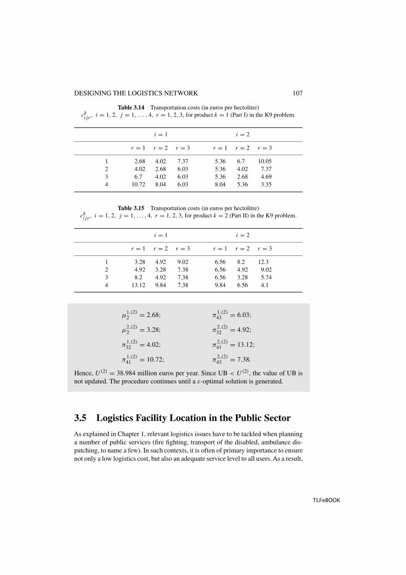
2,(2)43 = 7.38.

Hence, U(2) = 38.984 million euros per year. Since UB < U(2), the value of UB isnot updated. The procedure continues until a ε-optimal solution is generated.

3.5 Logistics Facility Location in the Public Sector

As explained in Chapter 1, relevant logistics issues have to be tackled when planninga number of public services (fire fighting, transport of the disabled, ambulance dis-patching, to name a few). In such contexts, it is often of primary importance to ensurenot only a low logistics cost, but also an adequate service level to all users. As a result,

TLFeBOOK


specific models have to be applied when locating public facilities. For example, inthe p-centre model described below, the service time of the most disadvantaged useris to be minimized, whereas in the location-covering model one has to determine theleast-cost set of facilities such that each user can be reached within a given maximumtravel time.

3.5.1 p-centre models

In the p-centre model the aim is to locate p facilities on a graph in such a way that themaximum travel time from a user to the closest facility is minimized. The p-centremodel finds its application when it is necessary to ensure equity in servicing usersspread on a wide geographical area.

The problem can be modelled on a directed, undirected or mixed graph G(V, A, E),where V is a set of vertices representing both user sites and road intersections, whileA and E (the set of arcs and edges, respectively) describe the road connections amongthe sites. Exactly p facilities have to be located either on a vertex or on an arc or edge.For p � 2, the p-centre model is NP-hard.

If G is a directed graph, there exists an optimal solution of the p-centre problemsuch that every facility location is a vertex (vertex location property). If G is undirectedor mixed, the optimal location of a facility could be on an internal point of an edge.In what follows, a solution methodology is described for the 1-centre problem. Thereader should consult specialized books for a discussion of the other cases. If G isdirected, the 1-centre is simply the vertex associated with the minimum value of themaximum travel time to all the other vertices. In the case of an undirected or mixedgraph, the 1-centre can correspond to a vertex or an internal edge point. To simplify thediscussion, we will refer only to the case of the undirected graph (A = ∅), althoughthe procedure can be easily applied in the case of mixed graph. For each (i, j) ∈ E, letaij be the traversal time of edge (i, j). Furthermore, for each pair of vertices i, j ∈ V ,denote by t

ji the shortest travel time between i and j , corresponding to the sum of the

travel times of the edges of the shortest path between i and j . Note that, on the basisof the definition of travel time, the result is

tji � aij , (i, j) ∈ E.

Finally, denote by τh(phk) the travel time along edge (h, k) ∈ E between vertexh ∈ V and a point phk of the edge. In this way, the travel time τh(phk) along the edge(h, k) between the vertex k ∈ V and phk results as (see Figure 3.9)

τk(phk) = ahk − τh(phk).

The 1-centre problem can be solved by the following algorithm proposed byHakimi.

Step 1. (Computation of the travel time.) For each edge (h, k) ∈ E and for eachvertex ∈ V , determine the travel time Ti(phk) from i ∈ V to a point phk of the

TLFeBOOK


kh

i

ti

h(phk)

phk

τh(phk)τ

h tik

Figure 3.9 Computation of the travel time Ti(phk) from an user i ∈ V to a facility in phk .

Ti (phk)ti + ahk

h k

ti + ahk

ti

phk

hti

k

h

k

Figure 3.10 Travel time Ti(phk) versus the position of point phk along edge (h, k).

edge (h, k) (see Figure 3.10):

Ti(phk) = min[thi + τh(phk), tki + τk(phk)]. (3.57)

Step 2. (Finding the local centre.) For each edge (h, k) ∈ E, determine the localcentre p∗

hk as the point on (h, k) minimizing the travel time from the most disad-vantaged vertex,

p∗hk = arg min max

i∈V{Ti(phk)},

where maxi∈V {Ti(phk)} corresponds to the superior envelope of the functionsTi(phk), i ∈ V (see Figure 3.11).

TLFeBOOK


i ∈V

* phkphkh k

max{Ti (phk)}

Figure 3.11 Determination of the local centre of edge (h, k) ∈ E.

Torre de Juan Abad

Infantes

Villahermosa

Villanuevade la Fuente

Albaladejo

Montiel

Puebla delPrincipe

Santa Cruzde los Canamos

TerrinchesTerrinchesTerrinches

Almedina

Infantes-Montielcrossing

1

23

4

6

7

8

10

9

11

5

Figure 3.12 Location problem in La Mancha region.

Step 3. (Determination of the 1-centre.) The 1-centre p∗ is the best local centre p∗hk ,

(h, k) ∈ E, i.e.

p∗ = arg min(h,k)∈E

{min max

i∈V{Ti(phk)}

}.

In the La Mancha region of Spain (see Figure 3.12) a consortium of town councils,located in an underpopulated rural area, decided to locate a parking place for ambu-lances. A preliminary examination of the problem revealed that the probability ofreceiving a request for service during the completion of a previous call was extremelylow because of the small number of the inhabitants of the zone. For this reason the

TLFeBOOK


Table 3.16 Vertices of La Mancha 1-centre problem.

Vertex Locality

1 Torre de Juan Abad2 Infantes3 Villahermosa4 Villanueva de la Fuente5 Albaladejo6 Terrinches7 Santa Cruz de los Canamos8 Montiel9 Infantes-Montiel crossing

10 Almedina11 Puebla del Principe

team responsible for the service decided to use only one vehicle. In the light of thisobservation, the problem was modelled as a 1-centre problem on a road network G

where all the connections are two-way streets (see Table 3.16). Travel times werecalculated assuming a vehicle average speed of 90 km/h (see Table 3.17).

Travel times tji , i, j ∈ V , are reported in Table 3.18. For each edge (h, k) ∈ E and

for each vertex i ∈ V the travel time Ti(phk) from vertex i to a point phk of the edge(h, k) can be defined through Equation (3.57). This enables the construction, for eachedge (h, k) ∈ E of the function maxi∈V {Ti(phk)}, whose minimum corresponds tothe local centre p∗

hk . For example, Figure 3.13 depicts the function maxi∈V {Ti(p23)},and Table 3.19 gives, for each edge (h, k) ∈ E, both the position of p∗

hk and the valuemaxi∈V {Ti(p

∗hk)}.

Consequently the 1-centre corresponds to the point p∗ on the edge (8, 10). There-fore, the optimal positioning of the parking place for the ambulance should be locatedon the road between Montiel and Almedina, at 2.25 km from the centre of Montiel.The villages least advantaged by this location decision are Villanueva de la Fuenteand Torre de Juan Abad, since the ambulance would take an average time of 11.5 minto reach them.

3.5.2 The location-covering model

In the location-covering model the aim is to locate a least-cost set of facilities in sucha way that each user can be reached within a maximum travel time from the closestfacility. The problem can modelled on a complete graph G(V1∪V2, E), where verticesin V1 and in V2 represent potential facilities and customers, respectively, and eachedge (i, j) ∈ E = V1 × V2 corresponds to a least-cost path between i and j .

TLFeBOOK


Table 3.17 Travel time (in minutes) on the road network edges in the La Mancha problem.

(i, j) aij (i, j) aij

(1,2) 12 (1,11) 8(2,3) 9 (2,9) 8(3,4) 11 (2,10) 9(4,5) 9 (3,9) 4(5,6) 2 (4,8) 10(6,7) 3 (5,8) 6(7,8) 4 (6,11) 5(8,9) 1 (7,10) 5(8,10) 7 (1,10) 6

(10,11) 4

Table 3.18 Travel times (in minutes) tji, i, j ∈ V , in the La Mancha problem.

i

j 1 2 3 4 5 6 7 8 9 10 11

1 0 12 18 23 15 13 11 13 14 6 82 12 0 9 19 15 16 13 9 8 9 133 18 9 0 11 11 12 9 5 4 12 164 23 19 11 0 9 11 14 10 11 17 165 15 15 11 9 0 2 5 6 7 10 76 13 16 12 11 2 0 3 7 8 8 57 11 13 9 14 5 3 0 4 5 5 88 13 9 5 10 6 7 4 0 1 7 119 14 8 4 11 7 8 5 1 0 8 12

10 6 9 12 17 10 8 5 7 8 0 411 8 13 16 16 7 5 8 11 12 4 0

Let fi, i ∈ V1, be the fixed cost of potential facility i; pj , j ∈ V2, the penaltyincurred if customer j is unserviced; tij , i ∈ V1, j ∈ V2, the least-cost travel timebetween potential facility i and customer j ; aij , i ∈ V1, j ∈ V2, a binary constantequal to 1 if potential facility i is able to serve customer j , 0 otherwise (given a user-defined maximum time T , aij = 1, if tij � T , i ∈ V1, j ∈ V2, otherwise aij = 0).The decision variables are binary: yi, i ∈ V1, is equal to 1 if facility i is opened, 0otherwise; zj , j ∈ V2, is equal to 1 if customer j is not served, otherwise it is 0.

The location-covering problem is modelled as follows:

Minimize ∑i∈V1

fiyi +∑j∈V2

pjzj (3.58)

TLFeBOOK


Table 3.19 Distances of the local centres p∗hk

from vertices h (in kilometres) andmaxi∈V {Ti(p

∗hk

)} (in minutes) in the La Mancha problem.

(h, k) γh(p∗hk

) maxi∈V {Ti(p∗hk

)} (h, k) γh(p∗hk

) maxi∈V {Ti(p∗hk

)}(1,2) 18.00 19.0 (1,11) 12.00 16.0(2,3) 6.00 17.0 (2,9) 12.00 14.0(3,4) 0.00 18.0 (2,10) 13.50 17.0(4,5) 13.50 15.0 (3,9) 6.00 14.0(5,6) 0.00 15.0 (4,8) 15.00 13.0(6,7) 3.75 13.5 (5,8) 9.00 13.0(7,8) 2.25 12.5 (6,11) 4.50 15.0(8,9) 0.00 13.0 (7,10) 0.00 14.0(8,10) 2.25 11.5 (1,10) 9.00 17.0

(10,11) 6.00 16.0

17

3.75 13.500.75 3.00 6.00 11.259.759.00

i ∈Vmax{Ti (p23)}

2 (p23)γ

Figure 3.13 Time maxi∈V {Ti(p23)} versusposition γ2(p23) of p23 in the La Mancha problem.


aij yi + zj � 1, j ∈ V2, (3.59)

yi ∈ {0, 1}, i ∈ V1,

zj ∈ {0, 1}, j ∈ V2.

The objective function (3.58) is the sum of the fixed costs of the open facilities andthe penalties corresponding to the unserviced customers. Constraints (3.59) imposethat, for each j ∈ V2, zj is equal to 1 if the facilities opened do not cover customer j

(i.e. if∑

i∈V1aij yi = 0).

TLFeBOOK


Table 3.20 Distances (in kilometres) between municipalities ofthe consortium in Portugal (Part I).

Almada Azenha Carregosa Corroios Lavradio

Almada 0.0 24.4 33.2 4.7 29.9Azenha 24.4 0.0 13.2 18.2 14.8Carregosa 33.2 13.2 0.0 27.1 11.1Corroios 4.7 18.2 27.1 0.0 23.8Lavradio 29.9 14.8 11.1 23.8 0.0Macau 39.0 15.4 13.9 32.9 16.1Moita 29.5 9.5 5.1 23.4 7.4Montijo 38.8 18.7 7.2 32.7 16.6Palmela 34.3 24.0 16.4 28.2 26.2Pinhal Novo 39.1 16.9 10.9 33.0 14.2

If all customers must be served (i.e. if the penalties pj are sufficiently high foreach j ∈ V2), variables zj , j ∈ V2, can be assumed equal to 0. Hence, the location-covering problem is a generalization of the well-known set covering problem and istherefore NP-hard.

Several variants of the location-covering model can be used in practice. For exam-ple, if fixed costs fi are equal for all potential sites i ∈ V1, it can be convenientto discriminate among all the solutions with the least number of open facilities theone corresponding to the least total travelling time, or to the most equitable demanddistribution among the facilities. In the former case, let xij , i ∈ V1, j ∈ V2, be abinary decision variable equal to 1 if customer j is served by facility i, 0 otherwise.The problem can be modelled as follows:

Minimize ∑i∈V1

Myi +∑i∈V1

∑j∈V2

tij xij (3.60)


aij xij � 1, j ∈ V2, (3.61)

∑j∈V2

xij � |V2|yi, i ∈ V1, (3.62)

yi ∈ {0, 1}, i ∈ V1, (3.63)

xij ∈ {0, 1}, i ∈ V1, j ∈ V2, (3.64)

where M is a large positive constant. Constraints (3.61) guarantee that all the cus-tomers j ∈ V2 are serviced, while constraints (3.62) ensure that if facility i ∈ V1 isnot set up (yi = 0), then no customer j ∈ V2 can be served by it.

TLFeBOOK


Table 3.21 Distances (in kilometres) between municipalities ofthe consortium in Portugal (Part II).

Macau Moita Montijo Palmela Pinhal Novo

Almada 39.0 29.5 38.8 34.3 39.1Azenha 15.4 9.5 18.7 24.0 16.9Carregosa 13.9 5.1 7.2 16.4 10.9Corroios 32.9 23.4 32.7 28.2 33.0Lavradio 16.1 7.4 16.6 26.2 14.2Macau 0.0 9.1 12.0 6.9 1.7Moita 9.1 0.0 10.6 11.7 7.2Montijo 12.0 10.6 0.0 19.0 10.3Palmela 6.9 11.7 19.0 0.0 8.8Pinhal Novo 1.7 7.2 10.3 8.8 0.0

In Portugal, a consortium of 10 municipalities (Almada, Azenha, Carregosa, Cor-roios, Lavradio, Macau, Moita, Montijo, Palmela, Pinhal Novo), located in the neigh-bourhood of Lisbon, has decided to improve its fire-fighting service. The personresponsible for the project has established that each centre of the community mustbe reached within 15 min from the closest fire station. Since the main aim is just toprovide a first help in case of fire, the decision maker has decided to assign a singlevehicle to each station. The annual cost of a station inclusive of the expenses of thepersonnel is €198 000. It is assumed that the average travelling speed is 60 km/heverywhere. In order to determine the optimal station location the location-coveringmodel (3.60)–(3.64) is used, where V1 = V2 = {Almada, Azenha, Carregosa, Cor-roios, Lavradio, Macau, Moita, Montijo, Palmela, Pinhal Novo}. Time coefficientstij , i ∈ V1, j ∈ V2, can be easily determined from the distances (in kilometres)reported in Tables 3.20 and 3.21. Coefficients aij , i ∈ V1, j ∈ V2, were obtainedfrom Tables 3.20 and 3.21. The minimum number of fire stations turns out to be two.The facilities are located in Almada and Moita. The fire station located in Almadaserves Corroios and Almada itself, the remaining ones are served by the fire stationlocated in Moita.

Another interesting variant of the location-covering model arises when one mustlocate facilities to ensure double coverage of demand points. A classic case is ambu-lance location when users are better protected if two ambulances are located withintheir vicinity. If one of the two ambulances has to answer a call, there will remain oneambulance to provide coverage.

3.6 Data Aggregation

Modelling and solving a location problem often requires a considerable amount ofdata. For instance, the number of demand points of a large food producer often exceeds

TLFeBOOK


several thousands. Similarly, the items marketed by a distribution firm can be aroundtens of thousands.Therefore, in order to keep computation times and hardware require-ments acceptable, data have to be aggregated. This can be done mainly in two ways.

Demand aggregation. Customers can be aggregated according to their position,service level or frequency of delivery. In the first case, demand points are clustered insuch a way that customers close to one another (e.g. customers having the same zipcode) are substituted by a customer zone. In the other cases, customers are aggregatedinto classes.

Item aggregation. Items are aggregated into a suitable number of product groups.This can be done according to their distribution pattern or their features (weight,volume, shape, cost, etc.). In the former case, products manufactured by the sameplants and supplied to the same customers are treated as a single commodity. Inthe latter case, similar items (e.g. variants of the same basic product model) areaggregated.

Whatever the aggregation method, the reduced problem can be modelled with fewervariables and constraints. In what follows, a demand aggregation method for the CPLmodel (see Section 3.3.1) is analysed. The demand points of a subset S ⊂ V2 areaggregated in the following way:

xij = xik, i ∈ V1, j ∈ S, k ∈ S.

Consequently, each point j ∈ S receives the same fraction of demand from eachfacility i ∈ V1. Let s be the customer zone resulting from the aggregation. Then theCPL model becomes:

Minimize ∑i∈V1

∑j∈(V2\S)∪{s}

cij xij +∑i∈V1

fiyi


xij = 1, j ∈ (V2 \ S) ∪ {s},∑

j∈(V2\S)∪{s}djxij � qiyi, i ∈ V1,

0 � xij � 1, i ∈ V1, j ∈ (V2 \ S) ∪ {s},yi ∈ {0, 1}, i ∈ V1,

wherecis =

∑j∈S

cij , i ∈ V1,

andds =

∑j∈S

dj .

TLFeBOOK


As a rule, the optimal solution value of the aggregated problem is worse than thatof the original problem. It is useful to evaluate an upper bound on the error maderesulting from the aggregation procedure. Let z∗

CPL and z(a)CPL be the costs of the

optimal solutions of the original problem and of the aggregate problem, respectively.

Property. The following relation holds,

z∗CPL � z

(a)CPL � z∗

CPL + ε,

where

ε =∑j∈S

maxi∈V1

{dj

∑r∈S cir∑

r∈S dr

− cij

}. (3.65)

Proof. In Equation (3.65),∑

r∈S cir represents the transportation cost when the wholedemand of customers in S is served by facility i ∈ V1, while dj /

∑r∈S dr represents

the fraction of the total demand of customers in S. The difference(dj

∑r∈S

cir

/ ∑r∈S

dr

)− cij

represents, therefore, the variation (positive, negative or zero) of the cost of assigningthe whole demand of customer j ∈ V2 to facility i ∈ V1 when the vertices of S areaggregated. Therefore, Equation (3.65) expresses the worst-case error made in theaggregation process as a sum of the maximum increases of the distribution costs ofthe various demand points in S.

It can be shown that bound (3.65) is tight, i.e. there are instances such that theaggregation error is nearly equal to ε.

If the demands of Brossard and Verdun are aggregated in the Goutte problem(see Section 3.3, where the maximum distance between plants and sales districts isassumed to be infinite), the worst-case error is, on the basis of Equation (3.65),

ε = ε1 + ε2 = 1578.92 Canadian dollars per year,

where

ε1 = maxi∈V1

{q1(ci1 + ci6)

(q1 + q6)− ci1

}= 789.46 Canadian dollars per year,

ε2 = maxi∈V1

{q6(ci1 + ci6)

(q1 + q6)− ci6

}= 789.46 Canadian dollars per year.

The above aggregation technique can be obviously extended to the case of K

disconnected subsets S1, . . . , SK .

TLFeBOOK


Property. An a priori upper bound on the error is given by

z∗CPL � z

(a)CPL � z∗

CPL +K∑

k=1

εk,

where

εk =∑j∈Sk

maxi∈V1

{dj

∑r∈Sk

cir∑r∈Sk

dr

− cij

}.

3.7 Questions and Problems

3.1 Illustrate why crude oil refineries are customarily located near home heatingand automotive fuel markets.

3.2 Describe how fixed costs fi , i ∈ V1, in the CPL model should be computedin order to take labour costs, property taxes and site-development costs intoaccount.

3.3 Your company has to close 20 of its 125 warehouses. Suppose the CPL hypothe-ses hold. How would you define V1? What is the value of p?

3.4 Modify the CPL model to take into account that a subset of already existingfacilities V ′

1 ⊆ V1 cannot be closed (but can be upgraded). Indicate the currentfixed cost and capacity of facility i ∈ V ′

1 as f ′i and q ′

i , respectively. Moreover,let f ′′

i and q ′′i be the fixed cost and capacity if facility i ∈ V ′

1 is upgraded,respectively.

3.5 Borachera is a major Spanish wine wholesaler currently operating two CDCs inSalamanca and Albacete, and a number of RDCs all over the Iberian peninsula.In order to reduce the overall logistics cost, the company wishes to redesign itsdistribution network by replacing its current RDCs with three (possibly new)RDCs. Based on a preliminary qualitative analysis, an RDC should be locatedin the Castilla-Leon region, either in Vallalolid, Burgos or Soria.A second RDCshould be located in the Extremadura region, either in Badajoz, Plasencia orCaceres. Finally, the third RDC should be located in the Argon region, eitherin Barbastro, Saragossa or Teruel. Transportation costs from RDCs to retailersare charged to retailers. Formulate the Borachera problem as a modified CPLmodel.

3.6 As illustrated in Section 3.3, when designing a distribution network it is cus-tomary to remove excessively long transportation links from the model in orderto allow for a timely delivery to customers. How should the CPL Lagrangianheuristic be modified in this case?

3.7 Modify the CPL Lagrangian heuristic for the case where demand is indivisible(i.e. a customer demand must be satisfied by a single warehouse). Is the modified

TLFeBOOK


heuristic still time-polynomial? How can it determine whether an instance ofthe modified problem is feasible?

3.8 Modify the TEMC model in Section 3.4 for the case where a customer canreceive shipments from different DCs if these shipments are for different com-modities. How should the proposed heuristics be changed in order to take thismodification into account?

3.9 Modify the location-covering model in order to determine, among the least-cost solutions, the one associated with the most equitable demand distributionamong the facilities.

3.10 Data aggregation is useful in facility location even if the available algorithmsare able to solve the original problems.Why? (Hint: recall that demand forecastsat the account and product levels are generally mediocre.)

3.8 Annotated Bibliography

An extensive literature review of strategic production-distribution models is presentedin the following article:

1. Vidal C and Goetschalckx M 1997 Strategic production-distribution models: acritical review with emphasis on global supply chain models. European Journalof Operational Research 98, 1–18.

An in-depth examination of location theory in a broader context is reported in thefollowing book:

2. Love RF, Morris JG and Wesolowsky GO 1988 Facilities Location. North-Holland, Amsterdam.

A review of the most important location-routing problems is presented in:

3. Laporte G 1988 Location-routing problems. In Vehicle Routing: Methods andStudies (ed. Golden BL and Assad AA). North-Holland, Amsterdam.

TLFeBOOK

TLFeBOOK

designing the logistics network - ieu.edu.trhomes.ieu.edu.tr/~aornek/wiley - introduction to...

Documents