designing effective improvement methods for scatter search

ORIGINAL PAPER

Designing effective improvement methods for scatter search:an experimental study on global optimization

Lars Magnus Hvattum • Abraham Duarte •

Fred Glover • Rafael Martı

Published online: 10 August 2012

� Springer-Verlag 2012

Abstract Scatter search (SS) is a metaheuristic frame-

work that explores solution spaces by evolving a set of

reference points. These points (solutions) are initially

generated with a diversification method and the evolution

of these reference points is induced by the application of

four methods: subset generation, combination, improve-

ment and update. In this paper, we consider the application

of the SS algorithm to the unconstrained global optimiza-

tion problem and study its performance when coupled with

different improvement methods. Specifically, we design

and implement new procedures that result by combining SS

with eight different improvement methods. We also pro-

pose an SS procedure (on the space of parameters) to

determine the values of the key search parameters used to

create the combined methods. We finally study whether

improvement methods of different quality have a direct

effect on the performance of the SS procedure, and whether

this effect varies depending on attributes of the function

that is minimized. Our experimental study reveals that the

improvement method is a key element in an effective SS

method for global optimization, and finds that the best

improvement methods for high-dimensional functions are

the coordinate method and two versions of scatter search

itself. More significantly, extensive computational tests

conducted with 12 leading methods from the literature

show that our resulting method outperforms competing

methods in the quality of both average solutions and best

solutions obtained.

Keywords Global optimization � Scatter search �Evolutionary methods

1 Introduction

The unconstrained continuous global optimization problem

may be formulated as follows:

Pð Þ Minimize f xð Þsubject to l� x� u; x; l; u 2 <n

;

where f(x) is a nonlinear function and x is a vector of con-

tinuous and bounded variables. Nonlinear functions provide

a good benchmark with hard instances to test optimization

methodologies. For detailed information regarding previous

work on global optimization we refer the reader to the

excellent web site of the ‘‘Soft Computing and Intelligent

Information Systems’’ research group at the University of

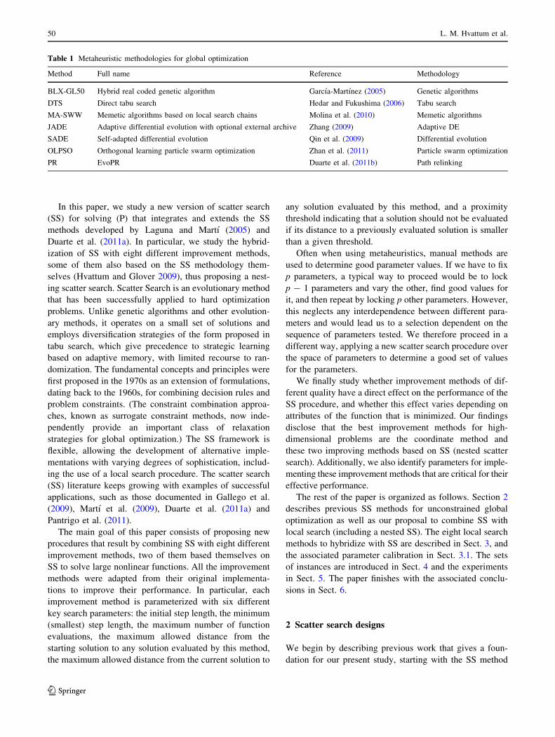
Granada (http://sci2s.ugr.es/eamhco). Most of the meta-

heuristic methodologies have been applied to unconstrained

global optimization as it is illustrated in Table 1, only

considering one method for each methodology.

L. M. Hvattum

Department of Industrial Economics and Technology

Management, The Norwegian University of Science

and Technology, Trondheim, Norway

e-mail: [email protected]

A. Duarte (&)

Departamento de Ciencias de la Computacion,

Universidad Rey Juan Carlos, Madrid, Spain


F. Glover

OptTek Systems, Inc., Boulder, CO, USA


R. Martı

Departamento de Estadıstica e Investigacion Operativa,

Universidad de Valencia, Valencia, Spain


123

Soft Comput (2013) 17:49–62

DOI 10.1007/s00500-012-0902-9

http://sci2s.ugr.es/eamhco

In this paper, we study a new version of scatter search

(SS) for solving (P) that integrates and extends the SS

methods developed by Laguna and Martı (2005) and

Duarte et al. (2011a). In particular, we study the hybrid-

ization of SS with eight different improvement methods,

some of them also based on the SS methodology them-

selves (Hvattum and Glover 2009), thus proposing a nest-

ing scatter search. Scatter Search is an evolutionary method

that has been successfully applied to hard optimization

problems. Unlike genetic algorithms and other evolution-

ary methods, it operates on a small set of solutions and

employs diversification strategies of the form proposed in

tabu search, which give precedence to strategic learning

based on adaptive memory, with limited recourse to ran-

domization. The fundamental concepts and principles were

first proposed in the 1970s as an extension of formulations,

dating back to the 1960s, for combining decision rules and

problem constraints. (The constraint combination approa-

ches, known as surrogate constraint methods, now inde-

pendently provide an important class of relaxation

strategies for global optimization.) The SS framework is

flexible, allowing the development of alternative imple-

mentations with varying degrees of sophistication, includ-

ing the use of a local search procedure. The scatter search

(SS) literature keeps growing with examples of successful

applications, such as those documented in Gallego et al.

(2009), Martı et al. (2009), Duarte et al. (2011a) and

Pantrigo et al. (2011).

The main goal of this paper consists of proposing new

procedures that result by combining SS with eight different

improvement methods, two of them based themselves on

SS to solve large nonlinear functions. All the improvement

methods were adapted from their original implementa-

tions to improve their performance. In particular, each

improvement method is parameterized with six different

key search parameters: the initial step length, the minimum

(smallest) step length, the maximum number of function

evaluations, the maximum allowed distance from the

starting solution to any solution evaluated by this method,

the maximum allowed distance from the current solution to

any solution evaluated by this method, and a proximity

threshold indicating that a solution should not be evaluated

if its distance to a previously evaluated solution is smaller

than a given threshold.

Often when using metaheuristics, manual methods are

used to determine good parameter values. If we have to fix

p parameters, a typical way to proceed would be to lock

p - 1 parameters and vary the other, find good values for

it, and then repeat by locking p other parameters. However,

this neglects any interdependence between different para-

meters and would lead us to a selection dependent on the

sequence of parameters tested. We therefore proceed in a

different way, applying a new scatter search procedure over

the space of parameters to determine a good set of values

for the parameters.

We finally study whether improvement methods of dif-

ferent quality have a direct effect on the performance of the

SS procedure, and whether this effect varies depending on

attributes of the function that is minimized. Our findings

disclose that the best improvement methods for high-

dimensional problems are the coordinate method and

these two improving methods based on SS (nested scatter

search). Additionally, we also identify parameters for imple-

menting these improvement methods that are critical for their

effective performance.

The rest of the paper is organized as follows. Section 2

describes previous SS methods for unconstrained global

optimization as well as our proposal to combine SS with

local search (including a nested SS). The eight local search

methods to hybridize with SS are described in Sect. 3, and

the associated parameter calibration in Sect. 3.1. The sets

of instances are introduced in Sect. 4 and the experiments

in Sect. 5. The paper finishes with the associated conclu-

sions in Sect. 6.

2 Scatter search designs

We begin by describing previous work that gives a foun-

dation for our present study, starting with the SS method

Table 1 Metaheuristic methodologies for global optimization

Method Full name Reference Methodology

BLX-GL50 Hybrid real coded genetic algorithm Garcıa-Martınez (2005) Genetic algorithms

DTS Direct tabu search Hedar and Fukushima (2006) Tabu search

MA-SWW Memetic algorithms based on local search chains Molina et al. (2010) Memetic algorithms

JADE Adaptive differential evolution with optional external archive Zhang (2009) Adaptive DE

SADE Self-adapted differential evolution Qin et al. (2009) Differential evolution

OLPSO Orthogonal learning particle swarm optimization Zhan et al. (2011) Particle swarm optimization

PR EvoPR Duarte et al. (2011b) Path relinking

50 L. M. Hvattum et al.

123

for (P) developed by Laguna and Martı (2005), which

excludes the use of an improvement method. The pseudo-

code in Fig. 1 shows their initial design. The method starts

with the creation of an initial reference set of solutions

(RefSet) ordered according to quality and initiates the

search by assigning the value of TRUE to the Boolean

variable NewSolutions. In step 3, NewSubsets is con-

structed and NewSolutions is switched to FALSE. Since we

are focusing our attention on subsets of size 2, the cardi-

nality of NewSubsets corresponding to the initial reference

set is given by b2 � bð Þ=2, which accounts for all pairs of

solutions in RefSet. The pairs in NewSubsets are selected

one at a time in lexicographical order and the solution-

combination method is applied to generate one or more

solutions in step 5. If a newly created solution improves

upon the worst solution currently in RefSet, the new solu-

tion replaces the worst and RefSet is reordered in step 6.

The NewSolutions flag is switched to TRUE and the subset

s that was just combined is deleted from NewSubsets in

steps 7 and 8, respectively.

Laguna and Martı (2005) tested several alternatives for

generating and updating the reference set. The combina-

tions generated by their approach are linear and limited to

joining pairs of solutions. They also tested the use of a two-

phase intensification.

Duarte et al. (2011a) extended the Laguna and Martı

study by incorporating two improvement methods within

their SS approach, the first one based on line searches

and the second one based on the well-known Nelder–

Mead method. As in Laguna and Martı (2005), the SS

algorithm of this work is based on the SS template

(Glover et al. 1998) which consists of the following five

methods:

a. A diversification-generation method to generate a

collection of diverse trial solutions, using an arbitrary

trial solution (or seed solution) as an input. In the

approach of the indicated studies, the range of each

variable is divided into four sub-ranges of equal size. A

random sub-range is selected with a probability that is

inversely proportional to its frequency count (the

number of times it has been selected before). Finally, a

random value is selected uniformly within the corre-

sponding sub-range, obtaining an initial solution. If the

difference between the new solution and any other

solution previously generated is smaller than a pre-

established threshold, the solution is discarded.

b. An improvement method to transform a trial solution into

one or more enhanced trial solutions. Neither the input

nor output solutions are required to be feasible, though

the output solutions will more usually be expected to

be so.

c. A reference set update method to build and maintain a

reference set consisting of the b ‘‘best’’ solutions found

(where the value of b is typically small, e.g. no more

than 20). New solutions are obtained by combining

solutions in the reference set as indicated below.

Solutions gain membership to the reference set according

to their quality or their diversity.

d. A subset-generation method to operate on the refer-

ence set, to produce several subsets of its solutions as a

basis for creating combined solutions. As in most SS

implementations, we limit the design of our present

study to combine pairs of solutions.

e. A solution-combination method to transform a given

subset of solutions produced by the subset-generation

method into one or more combined solution vectors.

Fig. 1 Outline of basic scatter

search

Designing effective improvement methods for scatter search 51

123

The combination method typically considers the line

through two solutions, x and y, given by the represen-

tation z(k) = x ? k (y - x) where k is a scalar weight.

In our implementation we consider three points in this

line: the convex combination z(1/2), and the exterior

solutions z(-1/3) and z(4/3). We evaluate these three

solutions and return the best as the result of combining

x and y.

The SS algorithm of Duarte et al. (2011a) differs in three

main ways from the design used by Laguna and Martı

(2005). First, in step 1 of Fig. 1, instead of directly

admitting a generated solution to become part of D, the

algorithm only admits those solutions x whose distance

d(x,D) to the solutions already in D is larger than a pre-

established threshold value, dthresh:

dðx;DÞ ¼ miny2D

dðx; yÞ� dthresh

Second, Duarte et al. (2011a) solves a max–min diversity

problem (Duarte and Martı 2007) to build the reference set

instead of generating a collection of diverse solutions by a

one-pass heuristic. Instead of the one-by-one selection of

diverse solutions, they proposed solving the maximum

diversity problem (MDP) that consists of finding, from a

given set of elements and corresponding distances between

elements, the most diverse subset of a given size. To use

the MDP within SS, we must recognize that the original set

of elements is given by P minus the |RefSet|/2 best solu-

tions. Also, the most diverse subset that we are asking the

MDP to construct is RefSet, which is already partially

populated with the |RefSet|/2 best solutions from P.

Therefore, the authors modified the D2 method (Glover

et al. 1998) to solve the special MDP for which some

elements have already been chosen.

Finally, the improvement method is selectively applied

to the best b solutions resulting from the combination

method (in the inner while loop of Fig. 1). Duarte et al.

(2011a) did not focus in particular on high-dimensional

functions (the number of dimensions is limited to 30 in

their study), but presented the currently best direct search

method for finding global solutions for low-dimensional

problems.

Hvattum and Glover (2009) present and evaluate several

direct search methods for finding local optima of high-

dimensional functions, including several classical methods

and two novel methods based on SS. The purpose of this

work was to illuminate the differences between the meth-

ods in terms of the number of function evaluations required

to find a locally optimal solution. It turns out that several

classical methods perform badly according to this criterion,

especially when the number of dimensions increases.

However, these classical methods are nevertheless used

quite frequently as central parts of metaheuristics designed

to find globally optimal solutions. An underlying motiva-

tion for the work of Hvattum and Glover (2009) was that if

a metaheuristic implementation employs a local improve-

ment method, the ability of metaheuristic to efficiently find

global optima of functions may depend on the ability of the

improvement method to find local optima.

As previously indicated, the current paper extends the

studies on scatter search (SS) described above by com-

bining (hybridizing) SS with eight different improvement

methods and determining values for key search parameters

used to create the combined methods.

We note that the successful design of the combined

methods depends heavily on both the identity and the

values of parameters studied. Our design includes adaptive

mechanisms for modifying the parameter values, and these

mechanisms and the analysis that provides initial parameter

values constitute one of the main contributions of our

study. Figure 2 gives an outline of our full scatter search

procedure with the steps for combining its component

algorithms. In the first while-loop (lines 1–3) the best

generated solutions are added to the initial reference set.

The second while-loop (lines 4–21) constitutes the main

iterations of the SS procedure. It is divided into two parts;

in the first one (lines 4–7) the reference set is completed by

adding diverse solutions to the quality solutions already in

it. In the second part (lines 8–20) the reference set is

evolved by applying the subset-generation method (lines 9

and 10), the combination method (lines 11–13), the

improvement method (lines 14 and 15) and the reference

set update method (lines 16–20). The procedure finishes

when a maximum number of function evaluations MaxEval

is reached.

3 The improvement method

From the perspective of the overall scatter search approach,

we consider the improvement method as a black box

optimizer subject to a set of search parameters. We have

included in our computational experience the following

eight different improvement methods. Note that the last

two are a scatter search implementations themselves and

therefore their inclusion in the general SS algorithm con-

stitutes a nested method.

• NM: Nelder–Mead simplex method

• MDS: multidirectional search

• CS: coordinate search method

• HJ: Hooke and Jeeves method

• SW: Solis and Wets’ algorithm

• ROS: Rosenbrock’s algorithm

• SSR: Scatter search with randomized subset combination

• SSC: Scatter search with clustering subset combination.


123

A brief description of these methods follows. The Nelder–

Mead, NM (Nelder and Mead 1965) is a classical direct

search method that has frequently been used as a sub-solver

in global optimization (Herrera et al. 2006). The method

works by creating a simplex around the initial point and

then applies four operations called reflection, expansion,

contraction and shrinkage to modify the simplex and

thereby improving the worst point of the simplex. Another

simplex-based method is the multidirectional search, MDS

(Wright 1996), which differs from NM in that it attempts to

improve the best point rather than the worst point in every

iteration, and that reflection, expansion, and contraction

works on the whole simplex rather than just the worst

point.

Coordinate search (CS) is a simple pattern search

(Kolda et al. 2003; Schwefel 1995) starting from a single

point and with a given step length. A search for impro-

ving points is made along each of the cartesian directions

using the current step length. If an improving point is

found it becomes the current point, otherwise, having

tested 2n points without improving the current step length

is reduced before the search continues. The method of

Fig. 2 Outline of the proposed

scatter search


123

Hooke and Jeeves (1961) is slightly more advanced than

CS. Having completed a search through all 2n directions

the method will make a tentative jump based on the

improvements found, but if no improvements are found in

the next cycle the jump is retracted before continuing as

normal.

Rosenbrock’s algorithm (Rosenbrock 1960) with impr-

ovements by Palmer (1969) also starts by searching along

each of the Cartesian directions, but modifies the directions

used based on previous improvements encountered. This

facilitates dealing with functions that have long, turning

valleys which the search follows to a local optimum. The

stochastic direct search SW of Solis and Wets (1981) does

not rely on a set of search directions, but generates a new

sample direction at every iteration based on n random

samples from normal distributions. The step length is

influenced by the variance of the normal distributions, and

the direction is influenced by the expected values of the

normal distributions. The expected values are based on a

bias that is updated depending on whether previous sam-

pled points have been successfully improving the current

solution.

Finally, the two direct search methods based on SS, as

developed in Hvattum and Glover (2009), maintain a

pool of solution points, with a special focus on the best

point which is always included when combining a subset

of solutions. The combination of solutions is made by

searching along a line that goes through the best point and

the centroid of the remaining points in the selected subset.

The two methods differ by the way that subsets are

selected for combination: SSR uses guided randomization

to find subsets, whereas SSC uses the k-clustering algo-

rithm (MacQueen 1967).

It is well known that, in the context of global optimi-

zation, improvement methods based on local search are

highly dependent on parameters such as the step length to

discretize the continuous domain. In our case we have three

sets of parameters: one concerning the main mechanisms of

the SS, one concerning the interaction between these

mechanisms and the improvement method, and one for the

improvement method itself. For the main mechanisms of

SS we use the same settings as in Duarte et al. (2011a), and

for settings specific to each direct search method we use

standard values, as in Hvattum and Glover (2009). In

addition, some values can be specified by the SS method

when using direct search as an improvement method. To

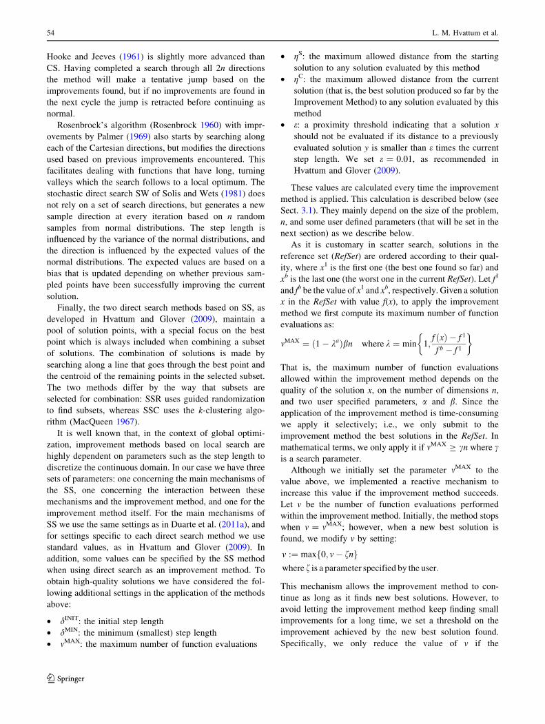
obtain high-quality solutions we have considered the fol-

lowing additional settings in the application of the methods

above:

• dINIT: the initial step length

• dMIN: the minimum (smallest) step length

• mMAX: the maximum number of function evaluations

• gS: the maximum allowed distance from the starting

solution to any solution evaluated by this method

• gC: the maximum allowed distance from the current

solution (that is, the best solution produced so far by the

Improvement Method) to any solution evaluated by this

method

• e: a proximity threshold indicating that a solution x

should not be evaluated if its distance to a previously

evaluated solution y is smaller than e times the current

step length. We set e = 0.01, as recommended in

Hvattum and Glover (2009).

These values are calculated every time the improvement

method is applied. This calculation is described below (see

Sect. 3.1). They mainly depend on the size of the problem,

n, and some user defined parameters (that will be set in the

next section) as we describe below.

As it is customary in scatter search, solutions in the

reference set (RefSet) are ordered according to their qual-

ity, where x1 is the first one (the best one found so far) and

xb is the last one (the worst one in the current RefSet). Let f1

and fb be the value of x1 and xb, respectively. Given a solution

x in the RefSet with value f(x), to apply the improvement

method we first compute its maximum number of function

evaluations as:

mMAX ¼ 1� kað Þbn where k ¼ min 1;f xð Þ � f 1

f b � f 1

� �

That is, the maximum number of function evaluations

allowed within the improvement method depends on the

quality of the solution x, on the number of dimensions n,

and two user specified parameters, a and b. Since the

application of the improvement method is time-consuming

we apply it selectively; i.e., we only submit to the

improvement method the best solutions in the RefSet. In

mathematical terms, we only apply it if mMAX C cn where cis a search parameter.

Although we initially set the parameter mMAX to the

value above, we implemented a reactive mechanism to

increase this value if the improvement method succeeds.

Let v be the number of function evaluations performed

within the improvement method. Initially, the method stops

when v = mMAX; however, when a new best solution is

found, we modify v by setting:

v :¼ max 0; v� fnf gwhere f is a parameter specified by the user:

This mechanism allows the improvement method to con-

tinue as long as it finds new best solutions. However, to

avoid letting the improvement method keep finding small

improvements for a long time, we set a threshold on the

improvement achieved by the new best solution found.

Specifically, we only reduce the value of v if the


123

improvement in the best solution found is larger than

v(f1 - f2) where f2 is the value of the second best solution

in the reference set and v is a search parameter.

The initial step length is set to dINIT = hdREF and the

minimum step length is set to dMIN = jdINIT where dREF is

the distance from the solution x to the closest solution in

the reference set and h and j are user specified parameters.

Finally, the calculation of gS and gC also involves the use

of specified parameters: s and /. We set gS = sdINIT, and

gC = /dINIT.

With respect to the memory structures, it must be noted

that although previously evaluated solutions are temporary

stored by the improvement method, only the starting

solution and the final solution are stored permanently. That

is, all solutions are stored during the execution of the

improvement method, to avoid multiple evaluations of very

similar solutions (as defined through e), and the starting and

final solutions are carried over to subsequent calls to the

improvement method. Since both the calculations of vMAX

and the use of v include references to nominal solution

values, the resulting SS is not a true direct search method,

as these should only require ordinal information about

function values (Lewis 2001).

3.1 Parameter calibration

As a result of the description above and considering that

some settings depend on others, we can conclude that the

following 9 parameters a, b, c, f, v, h, j, s and / need to be

determined. We note that there is a strong bias in the lit-

erature to consider it desirable for a method to have only a

very small number of parameters, or even better to have no

parameters at all. We support this view in principle, but

point out that if specific parameters have a meaningful role

within a method, then it would be imprudent to avoid

examining them and subjecting them to analysis. In addi-

tion, once values are assigned to parameters, they are

effectively turned into constants and the resulting algorithm

becomes parameter-free from the standpoint of the user.

The key is to identify a procedure capable of discovering

good parameter values to produce an effective algorithm.

We address this consideration in this section, using scatter

search itself as a strategy for parameter determination.

Since the local search procedures used as the improve-

ment method in our scatter search algorithm are very dif-

ferent, it is likely that they require different parameters

balancing how much effort is used in the improvement

method. For a relatively simple method it is better to use

more effort outside of the improvement method, whereas

an efficient improvement method may be allowed to spend

much effort improving selected solution points. Similarly,

if the function optimized has few local optima, using more

effort in the improvement method may be more beneficial

than if the function has many local optima. This is the

background for calibrating the parameters for each

improvement method separately and on functions similar to

those for which the method is eventually used.

For each of the nine parameters initial tests are made to

reveal intervals of values where the parameters make sense

(Lbound and Ubound in Table 2), as well as an initial guess

for a good set of parameter values. Let x be a vector of the

nine parameter values, and let l and u be vectors of lower

and upper bounds for parameter values giving a reasonable

performance, and let xINIT be the initial guess for a good set

of values. Let G be a set of functions g, and let vm(x,g) be

the number of function evaluations required by the SS

using improvement method m and parameter values x to

solve function g. To find final parameter values we can now

solve (P) while taking

f xð Þ ¼X

g2Gmm x; gð Þ:

Often when using metaheuristics, manual methods are

used to determine good parameter values. A typical way to

proceed would be to lock eight parameters and vary the

ninth, find good values for the ninth, and then repeat by

locking eight other parameters. However, this neglects

any interdependence between different parameters and

would lead us to a selection dependent on the sequence of

parameters tested. We therefore proceed in a different way,

applying a scatter search to determine a good set of values

for the parameters (i.e., since the problem of finding good

parameter values is cast in the framework of (P), we use the

SS method, bootstrapped with our initial guess xINIT).

When using SS to determine good parameters values,

the function f xð Þ ¼P

g2Gmm x; gð Þ is treated as any other

function, and we apply our SS procedure following a

normal execution: first generating a set of diverse values

for the parameters using the diversification-generation

method. Then, we use the reference set update method to

create the initial RefSet, selecting a specified number of

parameter sets (treated as solutions) based on their quality

and an additional number of such sets based on their

diversity (solving the min–max diversity problem as

described above). The SS iterations combine, improve and

replace solutions (sets of parameters) in the RefSet by

applying the subset-generation, improvement and combi-

nation methods, continuing as long as each iteration yields

an improvement. When the improvement method is applied

to a set of parameter values in the role of a solution x, the

method is started from the initial guess for good parameter

values. When evaluating a set of parameter values, each

g 2 G is solved using SS, with the improvement method

operating on the parameter set x. The SS method is halted

after a limited number of iterations (50,000), giving a

solution corresponding to a set of parameter values that has


123

received the best evaluation. This is repeated for each of

the eight improvement methods, in order to produce a set

of parameter values that is applicable to each method,

giving rise to the eight sets of parameter values reported in

Table 2.

Three sets of test instances are described in Sect. 4. We

have calibrated parameter settings separately for the

CEC05 instances and the LM-HG instances, by selecting a

few representative instances from each instance set as

G. We note from the parameter values in Table 2 that the

values for v, s and / are quite high. Additional testing has

revealed that ignoring these mechanisms of the algorithm

does not reduce the final solution quality obtained. Thus,

the overall algorithm can be simplified by the withdrawal

of the modification of the function evaluations’ number m.

4 Sets of instances

In order to test the search strategies and implementations

described in this paper, we consider three sets of instances.

In all these instances the optimum (minimum) objective

function value is known. Moreover, they are scalable for

any size of dimension. We consider the following features

for each function:

• unimodal functions where there is only one optimal

value within the domain and multimodal functions

where there is more than one (in general, much more

than one).

• non-shifted functions if the optimum value is located in

the centre of the search space and shifted functions if

the function is displaced.

• non-rotated functions if the optimum can be found

through the Cartesian axes, and rotated functions if the

function is rotated with respect to the Cartesian axes.

• separable functions as those than can be decomposed

in terms of mono-dimensional functions (one for each

dimension) and non-separable functions where this

decomposition is not possible.

Based on these features, the sets of instances previously

reported follow. The easiest instances are those that are

unimodal and non-shifted. On the other hand, the hardest

instances are those that are multimodal, shifted, rotated and

non-separable.

• LM-HG1: consists of 10 unimodal and shifted func-

tions, each one with dimension n = 2, 4, 8, 16, 32, 64,

128, 256 and 512. These instances have been previ-

ously used by Hvattum and Glover (2009), and are

based on functions listed in Laguna and Martı (2005).

They are modified so that the global optimum has a

value of 0, and most of them are separable. Their names

are: Branin, Booth, Matyas, Rosenbrock, Zakharov,

Trid, SumSquares, Sphere, Staircased-Rosenbrock and

Staircased-LogAbs.

• LM-HG2: consists of 16 multimodal and shifted

functions, each one with dimension n = 2, 4, 8, 16,

32, 64, 128, 256 and 512. These instances are generated

in the same way as LM-HG1, and are also based on

functions in Laguna and Martı (2005). Their names are:

B2, Easom, Goldstein and Price, Shubert, Beale,

SixHumpCamelBack, Schwefel, Colville, Perm(0.5),

Perm0(10), Rastrigin, Griewank, Powell, Dixon and

Price, Levy, and Ackley.

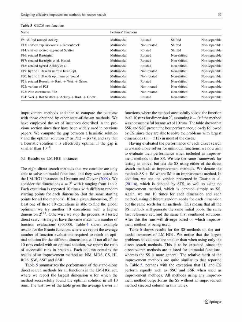
• CEC05: consists of 12 multimodal functions obtained

by composition and hybridization of functions in the

HG data set (biased, rotated, shifted and added). We

consider n = 10, n = 30 and n = 50. These instances

are described in detail in Suganthan (2005) under the

label ‘‘Never solved instances’’. Table 3 summarizes

the names and main features of each function.

5 Computational experiments

This section describes the computational experiments

we have performed to first test the efficiency of our SS

procedure, focusing in particular on the use of different

Table 2 Final parameters used in tests for the CEC05 instances

Lbound Ubound NM MDS SW HJ ROS CS SSC SSR

a 0.50 4.00 2.24 2.97 2.53 1.97 2.31 1.94 1.96 1.97

b 7.00 21.00 17.50 9.94 15.72 12.61 16.37 15.37 13.09 11.46

c 1.70 15.00 6.45 5.24 7.13 10.06 3.35 10.34 7.60 7.89

f 3.20 9.20 5.55 5.42 5.56 3.20 7.64 3.20 4.53 7.27

v 0.00 10.00 6.68 3.71 7.34 5.21 8.21 5.41 8.13 3.61

h 0.17 1.50 1.11 0.22 1.45 1.50 1.50 0.57 1.04 0.84

j 0.00 0.06 0.04 0.01 0.06 0.02 0.02 0.06 0.03 0.00

s 2.20 22.00 17.23 19.78 14.90 12.14 13.01 10.33 14.06 15.20

/ 7.00 16.00 10.15 13.83 11.70 11.00 7.79 11.03 9.77 13.09


123

improvement methods and then to compare the outcome

with those obtained by other state-of-the-art methods. We

have employed the set of instances described in the pre-

vious section since they have been widely used in previous

papers. We compute the gap between a heuristic solution

x and the optimal solution x* as |f(x) - f(x*)|, and say that

a heuristic solution x is effectively optimal if the gap is

smaller than 10-8.

5.1 Results on LM-HG1 instances

The eight direct search methods that we consider are only

able to solve unimodal functions, and they were tested on

the LM-HG1 instances in Hvattum and Glover (2009). We

consider the dimensions n = 2k with k ranging from 1 to 9.

Each execution is repeated 10 times with different random

starting points for each dimension (but the same starting

points for all the methods). If for a given dimension, 2k, at

least one of these 10 executions is able to find the global

optimum we try another 10 executions with a higher

dimension 2k?1. Otherwise we stop the process. All tested

direct search strategies have the same maximum number of

function evaluations (50,000). Table 4 shows example

results for the Branin function, where we report the average

number of function evaluations required to reach an opti-

mal solution for the different dimensions, n. If not all of the

10 runs ended with an optimal solution, we report the ratio

of successful runs in brackets. Each column contains the

results of an improvement method as: NM, MDS, CS, HJ,

ROS, SW, SSC and SSR.

Table 5 summarizes the performance of the stand-alone

direct search methods for all functions in the LM-HG1 set,

where we report the largest dimension n for which the

method successfully found the optimal solution in all 10

runs. The last row of the table gives the average k over all

functions, where the method successfully solved the function

in all 10 runs for dimension 2k, assuming k = 0 if the method

was not successful for any set of 10 runs. The table shows that

SSR and SSC present the best performance, closely followed

by CS, since they are able to solve the problems with largest

dimensions (n = 512) in most of the cases.

Having evaluated the performance of each direct search

as a stand-alone solver for unimodal functions, we now aim

to evaluate their performance when included as improve-

ment methods in the SS. We use the same framework for

testing as above, but test the SS using either of the direct

search methods as improvement methods. We denote the

methods SS ? IM where IM is an improvement method. In

addition, we test the version presented in Duarte et al.

(2011a), which is denoted by STS, as well as using no

improvement method, which is denoted simply as SS.

Again, we run 10 times for each dimension and each

method, using different random seeds for each dimension

but the same seeds for all methods. This means that all the

SS methods will generate the same initial pools, the same

first reference set, and the same first combined solutions.

After this the runs will diverge based on which improve-

ment method is being used.

Table 6 shows results for the SS methods on the uni-

modal instances of LM-HG1. We notice that the largest

problems solved now are smaller than when using only the

direct search methods. This is to be expected, since the

direct search methods are tailored for unimodal functions,

whereas the SS is more general. The relative merit of the

improvement methods are quite similar to that reported

in Table 5, perhaps with the exception that HJ and CS

perform equally well as SSC and SSR when used as

improvement methods. All methods using any improve-

ment method outperforms the SS without an improvement

method (second column in this table).

Table 3 CEC05 test functions

Name Features’ functions

F8: shifted rotated Ackley Multimodal Rotated Shifted Non-separable

F13: shifted exp.Griewank ? Rosenbrock Multimodal Non-rotated Shifted Non-separable

F14: shifted rotated expanded Scaffer Multimodal Rotated Shifted Non-separable

F16: rotated Rastriginl Multimodal Rotated Non-shifted Non-separable

F17: rotated Rastrigin et al. biased Multimodal Rotated Non-shifted Non-separable

F18: rotated hybrid Ackley et al. Multimodal Rotated Non-shifted Non-separable

F19: hybrid F18 with narrow basin opt. Multimodal Non-rotated Non-shifted Non-separable

F20: hybrid F18 with optimum on bound Multimodal Non-rotated Non-shifted Non-separable

F21: rotated Rosenb. ? Rast. ? Wei. ? Griew. Multimodal Rotated Non-shifted Non-separable

F22: variant of F21 Multimodal Non-rotated Non-shifted Non-separable

F23: Non continuous F22 Multimodal Non-rotated Non-shifted Non-separable

F24: Wei ? Rot Scaffer ? Ackley ? Rast. ? Griew. Multimodal Rotated Non-shifted Non-separable


123

5.2 Results on LM-HG2 instances

Table 7 reports results from the same test reported in

Table 6 using now the multimodal functions of set LM-

HG2. The relative results follow the same pattern as for the

unimodal functions, although the instances seem to be more

difficult and only slightly smaller dimensions can be solved

consistently. As in the previous experiment, the results in

this table clearly indicate that the scatter search algorithm

with either the CS, SSC or SSR exhibits the best results, with

Table 4 Number of function evaluations required by the improvement methods on the Branin function

n NM MDS CS HJ ROS SW SSR SSC

2 43.8 57.2 51.6 67.9 44.3 71.1 57.1 59.4

4 224.0 188.4 116.0 171.5 116.6 143.5 102.8 103.3

8 (0.0) 663.7 290.5 394.8 282.9 341.1 197.1 202.8

16 (0.0) 3,015.7 680.5 979.9 647.8 928.9 406.6 374.2

32 (0.0) 11,516.6 1,550.7 (0.9) 1,542.2 2,032.8 779.7 783.2

64 (0.0) 46,751.7 3,628.4 (0.9) 6,544.6 4,558.6 1,636.6 1,626.4

128 (0.0) (0.0) 8,031.5 (0.8) 28,666.7 9,922.3 3,448.8 3,443.7

256 (0.0) (0.0) 18,172.5 (0.6) (0.1) 24,043.6 7,173.4 7,184.6

512 (0.0) (0.0) (0.9) (0.7) (0.0) (0.2) 15,206.9 15,221.8

Table 5 Largest successful dimension for improvement methods on the LM-HG1 functions

f NM MDS SW HJ ROS CS SSC SSR

Branin 4 64 256 16 128 256 512 512

Booth 4 32 256 256 64 256 512 512

Matyas 4 16 256 128 128 256 256 256

Rosenbrock 4 0 4 0 32 2 32 64

Zakharov 4 16 32 16 64 16 32 32

Trid 4 8 16 16 32 16 16 16

SumSquares 4 32 64 512 64 512 512 512

Sphere 4 64 512 512 32 512 512 512

Stair-Ros. 0 0 0 2 32 2 32 64

Stair-LogAbs 2 32 2 256 4 512 512 512

Avg. k 1.7 3.8 5.1 5.4 5.4 6.1 7.2 7.4

The best results are highlighted in bold

Table 6 Largest successful dimension for SS on the LM-HG1 functions

f SS STS SS ? NM SS ? MDS SS ? SW SS ? HJ SS ? ROS SS ? CS SS ? SSC SS ? SSR

Branin 2 16 4 4 8 8 16 16 16 16

Booth 2 8 4 4 16 128 8 128 128 128

Matyas 2 16 8 4 32 128 32 256 256 256

Rosenbrock 0 4 2 2 2 4 4 4 4 2

Zakharov 2 8 4 4 8 16 8 16 8 8

Trid 2 8 4 4 8 32 8 16 16 16

SumSquares 2 16 4 4 16 32 32 32 32 32

Sphere 2 32 4 4 64 32 64 32 32 32

Stair-Ros. 0 4 2 2 2 4 2 2 4 2

Stair-LogAbs 0 4 0 0 0 128 2 128 256 256

Avg. k 0.7 3.2 1.7 1.6 3.0 4.7 3.3 4.7 4.8 4.6



123

an average value of the largest k (with n = 2k) that it is able

to solve (in all of the ten runs) of 3.1, 3.1 and 3.4, respec-

tively. Moreover, it improves the previous scatter search

algorithm, STS, which presents an average value of 2.9.

5.3 Results on CEC05 instances

To further analyze the consequences of using the different

improvement methods, we run experiments on the CEC05

instances as reported in Suganthan (2005). We use the same

random seeds for all the methods, and collect results for 25

runs for each function and dimension (following the exper-

imental design of that paper). Tables 8 and 9 show average

gap values for the functions using n = 10 and n = 50,

respectively. Each row in both tables reports the results after

1,000, 10,000, and 100,000 iterations, respectively.

Results in Tables 8 and 9 indicate that the choice of

improvement method is a key factor in the SS algorithm. In

CEC05 low-dimensional functions (n = 10), SS ? SW is

the best performer followed by SS ? SSC. Moreover, all

our variants give better results than the recent STS (Duarte

et al. 2011a). The difference between the methods becomes

evident already after 1,000 iterations. The performance on

high-dimensional functions (n = 50) reported in Table 9 is

perhaps more important. This time, the simplex-based

methods SS ? NM and SS ? MDS do not fare equally

well. The best performers are SS ? CS, SS ? SSC and

SS ? SSR, which is consistent with the results on the LM-

HG instances reported in Tables 6 and 7.

Having determined the best improving methods in the

previous experiments, we perform our final experiments

to compare the best variants, SS ? SSC, SS ? SSR,

SS ? SW and SS ? CS, with the best methods identified

in previous studies when executed over the set of instan-

ces CEC05. Specifically we consider STS (Duarte et al.

2011a), BLX-GL50 (Garcıa-Martınez 2005, BLX_MA

(Molina 2005), CoEVO (Posik 2005), JADE-adaptive dif-

ferential evolution (Zhang 2009), DMS-L-PSO (Liang

2005), EDA (Yuan 2005), G-CMA-ES (Auger 2005a),

k_PCX (Sinha et al. 2005), L-CMA-ES (Auger 2005b),

SaDE (Qin et al. 2009) and SPC-PNX (Ballester 2005).

Results for STS are computed a new based on the same

random seed as for the other SS variants, whereas results

for the other methods are gathered from the references

above. Note that all the other methods have been calibrated

for the CEC05 instances.

Following the guidelines in Suganthan (2005) we con-

sider first functions with n = 10 and then with n = 30. All

the methods are executed 25 independent times on each

instance and the maximum number of objective function

evaluation is limited to 10,000 or 100,000. We then record

the best gap value (minimum) and the average gap value

over the 25 runs for each instance. Tables 10 and 11 report

the average of the minimum (Min.) and the average of the

average (Avg.) optimality gap across the 12 CEC05

instances with n = 10 and n = 30, respectively. We do not

report the number of optima or any related value since none

of the methods considered is able to match any of them

Table 7 Largest successful dimension for SS on the LM-HG2 functions

f SS STS SS ? NM SS ? MDS SS ? SW SS ? HJ SS ? ROS SS ? CS SS ? SSC SS ? SSR

B2 0 2 2 2 4 8 4 16 16 32

Easom 0 2 2 2 2 2 4 2 4 4

Golds.&Price 0 8 2 2 4 8 8 8 8 8

Shubert 0 8 0 2 4 8 2 2 2 2

Beale 2 8 4 4 4 8 16 16 8 16

SixH.C.Back 2 16 2 4 16 32 16 32 64 64

Schwefel 0 8 2 2 2 4 0 2 2 2

Colville 0 4 0 0 4 8 4 8 8 4

Perm(0.5) 2 4 2 2 2 2 2 2 2 2

Perm0(10) 0 4 2 2 4 4 4 4 4 4

Rastrigin 0 16 0 0 2 4 2 2 2 2

Griewank 0 0 0 0 0 2 2 2 0 32

Powell 4 16 4 4 16 64 16 64 128 128

Dixon&Price 2 8 2 2 8 8 8 8 16 16

Levy 2 256 4 4 16 128 128 512 128 64

Ackley 0 8 0 0 0 32 8 32 32 32

Avg. k 0.4 2.9 0.9 1.0 1.9 3.1 2.5 3.1 3.1 3.4



123

(this is why these problems are called ‘‘Never solved

instances’’).

Results in Tables 10 and 11 clearly indicate that the SS

using the best choices of improvement methods is com-

petitive with, or even better than, the state-of-the-art

methods identified in recent publications. Specifically, for

n = 10 and 100,000 iterations, SS ? SW gives the best

results both when taking the best solution found among the

25 runs (185.9) and when taking the average (246.4). The

same holds true for n = 30, where it obtains in 100,000

iterations a minimum value of 399.8 and an average value

of 429.7. On the short term runs (10,000 iterations) with

n = 10, SS ? CS obtains the minimum value (222.4)

closely followed by L-CMA-ES (225.9), while the best

average value is achieved by EDA. With n = 30 and

10,000 iterations the best method in terms of minimum

value is G-CMA-ES (414.3) closely followed by SS ? SW

(419.4), and regarding average values, SaDE, SS ? SSR

and JADE obtain 484.6, 489.0 and 490.3, respectively.

We applied the nonparametric Friedman test for multi-

ple correlated samples to the best solutions obtained by our

best variant, SS ? SW, and each of the four methods

identified as the most recent and best: G-CMA-ES,

L-CMA-ES, JADE and SaDE. This test computes, for each

instance, the rank value of each method according to

solution quality (where rank 5 is assigned to the worst

Table 8 Average gap values over 25 runs on CEC05 instances with n = 10

Iterations SS STS SS ? NM SS ? MDS SS ? SW SS ? HJ SS ? ROS SS ? CS SS ? SSC SS ? SSR

1,000 780.1 773.2 645.5 737.5 552.7 652.9 627.4 575.7 613.1 601.9

10,000 733.1 585.9 425.8 565.5 366.0 426.7 449.8 415.4 398.2 432.1

100,000 646.8 399.0 297.1 351.8 246.4 309.3 341.1 298.4 291.6 314.4


Table 9 Average gap values over 25 runs on CEC05 instances with n = 50

Iterations SS STS SS ? NM SS ? MDS SS ? SW SS ? HJ SS ? ROS SS ? CS SS ? SSC SS ? SSR

1,000 1,029.3 1,041.8 993.7 1,050.1 859.2 753.7 830.7 752.8 765.1 758.6

10,000 908.8 839.1 725.7 898.2 640.6 632.8 634.9 635.0 643.6 617.6

100,000 824.0 662.4 623.9 749.9 563.2 573.5 572.6 532.2 523.0 527.9


Table 10 CEC05 test problems with n = 10

Method 10,000 iterations 100,000 iterations

Min. Avg. Min. Avg.

SS ? SSR 286.8 432.1 209.1 314.4

SS ? SSC 233.2 398.2 187.4 291.6

SS ? CS 222.4 415.4 205.2 298.4

SS ? SW 247.2 366.0 185.9 246.4

STS 336.8 585.9 242.3 399.0

G-CMA-ES 260.0 419.4 256.0 265.3

EDA 287.1 335.1 269.4 300.6

BLX-MA 315.5 445.1 306.2 430.1

SPC-PNX 279.6 391.0 206.0 309.9

BLX-GL50 272.8 341.0 257.2 319.0

L-CMA-ES 225.9 655.8 202.7 411.1

JADE 250.5 420.5 207.9 390.7

K-PCX 488.0 564.4 257.4 475.6

CoEVO 437.5 623.5 268.3 465.4

SaDE 286.4 375.7 246.3 308.8

DMS-L-PSO 356.9 477.0 244.4 392.3


Table 11 CEC05 test problems with n = 30

Method 10,000 iterations 100,000 iterations

Min. Avg. Min. Avg.

SS ? SSR 436.2 489.0 420.4 441.7

SS ? SSC 437.4 493.3 420.3 438.7

SS ? CS 430.9 509.4 420.4 441.5

SS ? SW 419.4 490.6 399.8 429.7

STS 617.0 752.8 415.3 550.9

G-CMA-ES 414.3 526.8 405.7 493.0

EDA 1,1951.1 26,418.8 653.6 934.7

BLX-MA 443.9 502.4 410.7 457.2

SPC-PNX 637.6 850.1 414.8 430.0

BLX-GL50 474.8 545.9 433.0 507.5

L-CMA-ES 447.6 722.6 404.6 617.0

JADE 437.2 490.3 419.2 480.2

K-PCX 27,719.7 108,602.9 866.1 2257.2

SaDE 457.6 484.6 428.1 439.3

CoEVO 749.6 822.0 625.3 734.5



123

method and rank 1 to the best one). We use the average

value over the 25 runs obtained with each method on each

of the 12 functions with n = 10 and n = 30, respectively.

Then, it calculates the average rank values of each method

across all the instances solved. If the averages differ

greatly, the associated p value or significance will be small.

The resulting p value of 0.000 obtained in this experiment

clearly indicates that there are statistically significant dif-

ferences among the five methods tested. Specifically, the

rank values produced by this test are, SS ? SW (2.29),

G-CMA-ES (2.40), SaDE (3.18), JADE (3.32) and

L-CMA-ES (3.81), confirming the superiority of our scatter

search algorithm.

Considering that SS ? SW and G-CMA-ES obtain very

similar rank values, we compared both with two well-known

nonparametric tests for pairwise comparisons: the Wilcoxon

test and the Sign test. The former one answers the question:

do the two samples (solutions obtained with SS ? SW and

G-CMA-ES in our case) represent two different populations?

The resulting p value of 0.236 indicates that the values

compared could come from the same method. On the other

hand, the Sign test computes the number of instances on

which an algorithm supersedes another one. The resulting

p value of 0.551 indicates that there is no clear winner

between SS ? SW and G-CMA-ES on the instances con-

sidered in our study. If we apply these two pairwise tests to

compare SS ? SW and SaDE we obtain a p value of 0.005

and 0.009, respectively, indicating that there are significant

differences between both methods.

6 Conclusions

We have described the development and implementation of

a Scatter Search algorithm for unconstrained nonlinear

optimization, identifying eight direct search optimizers that

we have applied as the improvement method within the

scatter search framework. Six of them are classic direct

search methods known from the literature, whereas two

were recently developed especially for high-dimensional

unimodal functions (Hvattum and Glover 2009). The per-

formance of these improvement methods is managed by

means of nine key search parameters, which incorporate

adaptive mechanisms and whose initial values we have

determined based on a series of experiments utilizing our

scatter search algorithm as a bootstrapping method to

identify effective parameter settings.

Comparative tests are performed on a set of 38 test

problems from three sources: unimodal (LM-HG-1), mul-

timodal (LM-HG2) and composed (CEC05), with the

number of variables ranging from 2 to 512. Most of these

instances have been previously identified as very hard to

solve. Our experimentation shows that the improvement

method is a key element in determining the relative per-

formance of alternative scatter search implementations.

Within our overall SS algorithm, which embeds the

improving method as a parameter-controlled subroutine,

the best performing improvement method for functions

with low dimension (n B 30) is the Solis and Wets algo-

rithm. For functions of higher dimensions (n C 50), the

best performance comes from coordinate search and two

improving methods based on scatter search itself. The two

scatter search improving methods demonstrate an ability to

yield the most effective performances for all of the three

different instance sets. Moreover, the extensive comparison

with 12 leading methods discloses that our overall scatter

search procedure (containing the improving methods by the

special designs we have developed) obtains solutions of

exceptionally high quality for unconstrained global opti-

mization problems.

In particular, for both n = 10 and n = 30, and using

100,000 iterations, our SS ? SW procedure obtains the

best results of all methods, as measured both by the best

solution found over 25 runs and by the average of these

solutions. The benchmark results we have established for

best and average solutions to larger problems additionally

provide a foundation to evaluate the performance of other

algorithms that may be applied to these challenging prob-

lem instances.

Acknowledgments This research has been partially supported by

the Ministerio de Ciencia e Innovacion of Spain (TIN2009-07516 and

TIN2012-35632). The authors thank the anonymous referees for

suggestions and comments that improved on the first version of this

paper.

References

Auger A, Hansen N (2005a) A restart CMA evolution strategy with

increasing population size. In: Proceedings of 2005 IEEE

congress on evolutionary computation (CEC’2005), pp 1769–

1776

Auger A, Hansen N (2005b) Performance evaluation of an advanced

local search evolutionary algorithm. In: Proceedings of 2005

IEEE congress on evolutionary computation (CEC’2005),

pp 1777–1784

Ballester PJ, Stephenson J, Carter N, Gallagher K (2005) Real-

parameter optimization performance study on the CEC-2005

benchmark with SPC-PNX. In: Proceedings of 2005 IEEE

congress on evolutionary computation (CEC’2005), pp 498–505

Duarte A, Martı R (2007) Tabu search for the maximum diversity

problem. Eur J Oper Res 178:71–84

Duarte A, Martı R, Glover F, Gortazar F (2011a) Hybrid scatter tabu

search for unconstrained global optimization. Ann Oper Res

183:95–123

Duarte A, Martı R, Gortazar F (2011b) Path relinking for large scale

global optimization. Soft Comput 15:2257–2273

Gallego M, Duarte A, Laguna M, Martı R (2009) Hybrid heuristics

for the maximum diversity problem. Comput Optim Appl

44(3):411–426


123

Garcıa-Martınez C, Lozano M (2005) Hybrid real-coded genetic

algorithms with female and male differentiation. In: Proceedings of

2005 IEEE congress on evolutionary computation (CEC’2005),

pp 896–903

Glover F, Kuo CC, Dhir KS (1998) Heuristic algorithms for the

maximum diversity problem. J Inf Optim Sci 19(1):109–132

Hedar A, Fukushima M (2006) Tabu search directed by direct search

methods for nonlinear global optimization. Eur J Oper Res 170(2):

329–349

Herrera F, Lozano M, Molina D (2006) Continuous scatter search: an

analysis of the integration of some combination methods and

improvement strategies. Eur J Oper Res 169:450–476

Hooke R, Jeeves TA (1961) Direct search solution of numerical and

statistical problems. J Assoc Comput Mach 8:212–229

Hvattum LM, Glover F (2009) Finding local optima of high-

dimensional functions using direct search methods. Eur J Oper

Res 195:31–45

Kolda TG, Lewis RM, Torczon VJ (2003) Optimization by direct

search: new perspectives on some classical and modern methods.

SIAM Rev 45:385–482

Laguna M, Martı R (2005) Experimental testing of advanced scatter

search designs for global optimization of multimodal functions.

J Glob Optim 33:235–255

Lewis RM, Torczon VJ, Trosset MW (2001) Direct search methods:

then and now. Bartholomew-Biggs M, Ford J, Watson L (eds)

Numerical analysis 2000 vol 4, Elsevier, pp 191–207

Liang JJ, Suganthan PN (2005) Dynamic multi-swarm particle swarm

optimizer with local search. In: Proceedings of 2005 IEEE


MacQueen JB (1967) Some methods for classification and analysis of

multivariate observations. In: LeCam LM, Neyman N (eds)

Proceedings of 5th Berkeley symposium on mathematical

statistics and probability, University of California Press, Berke-

ley, pp 281–297

Martı R, Duarte A, Laguna M (2009) Advanced scatter search for the

max-cut problem. INFORMS J Comput 21(1):26–38

Molina D, Herrera F, Lozano M (2005) Adaptive local search

parameters for real-coded memetic algorithms. In: Proceedings of


pp 888–895

Molina D, Lozano M, Garcıa-Martınez C, Herrera F (2010) Memetic

algorithms for continuous optimization based on local search

chains. Evol Comput 18(1):27–63

Nelder JA, Mead R (1965) A simplex method for function minimi-

zation. Comput J 7:308–313

Palmer JR (1969) An improved procedure for orthogonalising the

search vectors in Rosenbrock’s and Swann’s direct search

optimisation methods. Comput J 12:69–71

Pantrigo JJ, Martı R, Duarte A, Pardo EG (2011) Scatter search for

the cutwidth problem. Ann Oper Res. doi:10.1007/s10479-

011-0907-2

Posik P (2005) Real-parameter optimization using the mutation step

co-evolution. In: Proceedings of 2005 IEEE congress on

evolutionary computation (CEC’2005), pp 872–879

Qin AK, Huang VL, Suganthan PN (2009) Differential evolution

algorithm with strategy adaptation for global numerical optimi-

zation. IEEE Trans Evol Comput 13(2):398–417

Ronkkonen J, Kukkonen S, Price KV (2005) Real-parameter optimi-

zation with differential evolution. In: Proceedings of 2005 IEEE


Rosenbrock HH (1960) An automatic method for finding the greatest

or least value of a function. Comput J 3:175–184

Schwefel HP (1995) Evolution and optimum seeking. Wiley-

Interscience

Sinha A, Tiwari S, Deb K (2005) A population-based, steady-state

procedure for real-parameter optimization. In: Proceedings of


pp 514–521

Solis FJ, Wets RJ-B (1981) Minimization by random search

techniques. Math Oper Res 6:19–30

Suganthan PN, Hansen N, Liang JJ, Deb K, Chen Y-P, Auger A,

Tiwari S (2005) Problem definitions and evaluation criteria for

the CEC 2005 special session on real-parameter optimization.

Technical report, Nanyang Technological University, Singapore

and KanGAL Report Number 2005005 (Kanpur Genetic Algo-

rithms Laboratory, IIT Kanpur)

Wright MH (1996) Direct search methods: once scorned, now

respectable. In: Griffiths F, Watson GA (eds) Numerical analysis

1995. Addison Wesley Longman, Harlow, pp 191–208

Yuan B, Gallagher M (2005) Experimental results for the special

session on real-parameter optimization at CEC 2005: a simple,

continuous EDA. In: Proceedings of 2005 IEEE congress on

evolutionary computation (CEC’2005), pp 1792–1799

Zhan Z-H, Zhang J, Li Y, Shi Y-H (2011) Orthogonal learning particle

swarm optimization. IEEE Trans Evol Comput 15(6):832–847

Zhang J, Sanderson AC (2009) JADE: adaptive differential evolution

with optional external archive. IEEE Trans Evol Comput

13(5):945–958


123

http://dx.doi.org/10.1007/s10479-011-0907-2

http://dx.doi.org/10.1007/s10479-011-0907-2

designing effective improvement methods for scatter search

Documents