designing data center networks for high throughput
TRANSCRIPT

DESIGNING DATA CENTER NETWORKS FOR HIGH THROUGHPUT
BY
ANKIT SINGLA
DISSERTATION
Submitted in partial fulfillment of the requirementsfor the degree of Doctor of Philosophy in Computer Science
in the Graduate College of theUniversity of Illinois at Urbana-Champaign, 2015
Urbana, Illinois
Doctoral Committee:
Associate Professor P. Brighten Godfrey, Chair and Director of ResearchAssociate Professor Indranil GuptaProfessor Klara NahrstedtProfessor Scott Shenker, University of California at Berkeley, ICSI Berkeley

Abstract
Data centers with tens of thousands of servers now support popular Internet services, scientific research, as
well as industrial applications. The network is the foundation of such facilities, giving the large server pool
the ability to work together on these applications. The network needs to provide high throughput between
servers to ensure that computations are not slowed down by network bottlenecks, with servers waiting on
data from other servers. This work address two broad, related questions about high-throughput data center
network design: (a) how do we measure and benchmark various network designs for throughput? and (b)
how do we design such networks for near-optimal throughput?
The problem of designing high-throughput networks has received a lot of attention, with multiple inter-
esting architectures being proposed every year. However, there is no clarity on how one should benchmark
these networks and how they compare to each other. In fact, this work shows that commonly used measure-
ment approaches, in particular, cut-metrics like bisection bandwidth, do not predict throughput accurately.
In contrast, we directly evaluate the throughput of networks on both uniform and (heretofore unknown)
nearly-worst-case traffic matrices, and include here a comparison of 10 networks using this approach.
Further, prior work has not addressed a fundamental question: how far are we from throughput-optimal
design? In this work, we propose the first upper bound on network throughput for any topology with
identical switches. Although designing optimal topologies is infeasible, we demonstrate that random graphs
achieve throughput surprisingly close to this bound – within a few percent at the scale of a few thousand
servers for uniform traffic.
Our approach also addresses important practical concerns in the design of data center networks, such
as incremental expansion and heterogeneous design – as more and varied equipment is added to a data
center over the years in response to evolving needs, how do we best accommodate such equipment? Our
networks can achieve the same incremental growth at 40% of the expense such growth would incur with past
techniques for Clos networks. Further, our approach to designing heterogeneous topologies (i.e., where all
ii

the network switches are not identical) achieves 43% higher throughput than a comparable VL2 topology, a
heterogeneous network already deployed in Microsoft’s data centers.
We acknowledge that the use of random graphs also poses challenges, particularly with regards to ef-
ficient routing and physical cabling. We thus present here high-efficiency routing and cabling schemes for
such networks as well.
iii

To my family and friends
iv

Acknowledgments
I owe a great debt to my adviser, P. Brighten Godfrey. His mentorship has been invaluable throughout my
graduate studies. He has given me guidance, but also great freedom, and I have always looked forward to
our meetings and discussions. He has served as a role model not only in terms of research success, but also
as a wonderful person. At research conferences, innumerable folks have extended a certain warmth to me
on learning that he is my adviser, and that has always struck me as impressive.
My research collaborators have, of course, been instrumental in my work, and I have learnt a lot from
them. George Candea, Admela Jukan, and Ashwin Gumaste witnessed and supported my first, uncertain
steps into research. I was less committed than desirable, and I thank them for their patience. The first
published research output I produced came from work with Katerina Argyraki and Petros Maniatis. I greatly
enjoyed my work as Katerina’s intern, and continue to enjoy following her work. Over my PhD, I got
the opportunity to work with a large number of smart and wonderful people at UIUC, Intel Labs, NEC
Labs, ICSI Berkeley, IBM Research Austin, Duke University, as well as collaborators I came into contact
with through these first-degree connections. A special thanks is owed to Brighten Godfrey, Chi-Yao Hong,
Sangeetha Abdu Jyothi, Alexandra Kolla, and Lucian Popa, collaborations with whom produced the results
included in this thesis. Participating in the creative process that is research with these people will, I hope,
form enduring connections. Scott Shenker and Bruce Maggs have also been great mentors for me. In spite
of being so accomplished, they have graciously tolerated my humor, sometimes at their expense; I have
great regard for both of them. All of these people have contributed to my success, and in moulding me as a
researcher and person. Katerina Argyraki, John Carter, Brighten Godfrey, Bruce Maggs, and Scott Shenker
also helped make my academic job search a success, for which I’m immensely grateful. I also wish to thank
my dissertation committee members, Brighten Godfrey, Indranil Gupta, Klara Nahrstedt, and Scott Shenker,
for their useful feedback and their encouragement.
Besides being a great collaborator, Chi-Yao Hong has also been a great friend, and I have missed him
v

since his graduation and departure from Illinois; we undertook several fun adventures together, and I re-
member these often1. Support from fellow students and colleagues has been crucial to my progress and
happiness over the years. This includes not only the network-systems grads and faculty at Illinois, but many
others at Illinois and other places. They have asked probing questions, and made useful suggestions.
I am also thankful to the NSF, Cisco, and Google, for funding my work.
I have been extremely fortunate in being able to make friends across a variety of academic departments
and pursuits, and you are too many to list. I have shared housing with some of you, countless meals and
movies, road trips and adventures, dancing, music and singing, and lots of hilarity. Some of you became
my friends starting with our multiple chance encounters on public transport! Nevertheless, I feel compelled
to mention Nick Easter and Darienne Ciuro, friendships with whom have spanned the entirety of my stay
here. Also, Itxaso Rodriguez, who fed me lots of her delicious food2. I greatly enjoy her brutally honest,
yet somehow comical, approach to life.
A lot of my good friends from before graduate school have maintained contact all these years, and I look
forward to the same in the future. Support from Aditya Parameswaran and Prasang Upadhyaya over my job
search was particularly valuable.
I have, of course, missed my family here. My parents and my brother have provided a nurturing and
loving environment throughout my life, and have led me where I stand today. With the completion of this
endeavor, I finally join all of them in having post-graduate degrees!
1At Yellowstone National Park, I comment on our sighting of a bison: “Such an impressive, odd, large animal.”, to whichChi-Yao responds: “Looks delicious; it’d make so many burgers!!”
2Itxaso: “I am bored; if you tell me what you want, I’ll cook it for you.”
vi

TABLE OF CONTENTS
Chapter 1 Introduction . . . . . . . . . . . . . . . . . . . . . . . . . . . . . . . . . . . . . . . . . 1
Chapter 2 Background and related work . . . . . . . . . . . . . . . . . . . . . . . . . . . . . . . . 52.1 Network topology design . . . . . . . . . . . . . . . . . . . . . . . . . . . . . . . . . . . . 52.2 Evaluation of network topologies . . . . . . . . . . . . . . . . . . . . . . . . . . . . . . . . 8
Chapter 3 How do we evaluate topologies? . . . . . . . . . . . . . . . . . . . . . . . . . . . . . . . 103.1 Metrics for throughput . . . . . . . . . . . . . . . . . . . . . . . . . . . . . . . . . . . . . 12
3.1.1 Throughput defined . . . . . . . . . . . . . . . . . . . . . . . . . . . . . . . . . . . 123.1.2 Bisection bandwidth defined . . . . . . . . . . . . . . . . . . . . . . . . . . . . . . 133.1.3 Bisection bandwidth is the wrong metric . . . . . . . . . . . . . . . . . . . . . . . . 133.1.4 Sparsest cut defined . . . . . . . . . . . . . . . . . . . . . . . . . . . . . . . . . . . 143.1.5 Sparsest cut is the wrong metric . . . . . . . . . . . . . . . . . . . . . . . . . . . . 153.1.6 Aside: Are cut metrics useful at all? . . . . . . . . . . . . . . . . . . . . . . . . . . 173.1.7 Towards a throughput metric . . . . . . . . . . . . . . . . . . . . . . . . . . . . . . 173.1.8 Summary and implications . . . . . . . . . . . . . . . . . . . . . . . . . . . . . . . 20
3.2 Experimental evaluation . . . . . . . . . . . . . . . . . . . . . . . . . . . . . . . . . . . . 213.2.1 Methodology . . . . . . . . . . . . . . . . . . . . . . . . . . . . . . . . . . . . . . 213.2.2 Evaluation of the metrics . . . . . . . . . . . . . . . . . . . . . . . . . . . . . . . . 233.2.3 Evaluation of topologies . . . . . . . . . . . . . . . . . . . . . . . . . . . . . . . . 27
3.3 Comparison with related work . . . . . . . . . . . . . . . . . . . . . . . . . . . . . . . . . 323.4 Conclusion . . . . . . . . . . . . . . . . . . . . . . . . . . . . . . . . . . . . . . . . . . . 34
Chapter 4 Homogeneous topology design . . . . . . . . . . . . . . . . . . . . . . . . . . . . . . . 354.1 Jellyfish topology . . . . . . . . . . . . . . . . . . . . . . . . . . . . . . . . . . . . . . . . 384.2 Jellyfish topology properties . . . . . . . . . . . . . . . . . . . . . . . . . . . . . . . . . . 41
4.2.1 Efficiency . . . . . . . . . . . . . . . . . . . . . . . . . . . . . . . . . . . . . . . . 424.2.2 Flexibility . . . . . . . . . . . . . . . . . . . . . . . . . . . . . . . . . . . . . . . . 464.2.3 Failure resilience . . . . . . . . . . . . . . . . . . . . . . . . . . . . . . . . . . . . 49
4.3 Near-optimality of Jellyfish . . . . . . . . . . . . . . . . . . . . . . . . . . . . . . . . . . . 504.3.1 Topologies with higher throughput than Jellyfish? . . . . . . . . . . . . . . . . . . . 53
4.4 Conclusion . . . . . . . . . . . . . . . . . . . . . . . . . . . . . . . . . . . . . . . . . . . 55
Chapter 5 Heterogeneous topology design . . . . . . . . . . . . . . . . . . . . . . . . . . . . . . . 565.1 Simulation methodology . . . . . . . . . . . . . . . . . . . . . . . . . . . . . . . . . . . . 575.2 Heterogeneous port counts . . . . . . . . . . . . . . . . . . . . . . . . . . . . . . . . . . . 595.3 Heterogeneous line-speeds . . . . . . . . . . . . . . . . . . . . . . . . . . . . . . . . . . . 62
vii

5.4 Explaining throughput results . . . . . . . . . . . . . . . . . . . . . . . . . . . . . . . . . . 635.4.1 Experiments . . . . . . . . . . . . . . . . . . . . . . . . . . . . . . . . . . . . . . 645.4.2 Analysis . . . . . . . . . . . . . . . . . . . . . . . . . . . . . . . . . . . . . . . . 66
5.5 Improving VL2 . . . . . . . . . . . . . . . . . . . . . . . . . . . . . . . . . . . . . . . . . 695.6 Other traffic matrices . . . . . . . . . . . . . . . . . . . . . . . . . . . . . . . . . . . . . . 715.7 Conclusion . . . . . . . . . . . . . . . . . . . . . . . . . . . . . . . . . . . . . . . . . . . 71
Chapter 6 Systems challenges: routing and cabling . . . . . . . . . . . . . . . . . . . . . . . . . . 726.1 ECMP is not enough . . . . . . . . . . . . . . . . . . . . . . . . . . . . . . . . . . . . . . 726.2 k-Shortest-Paths with MPTCP . . . . . . . . . . . . . . . . . . . . . . . . . . . . . . . . . 746.3 Implementing k-Shortest-Path routing . . . . . . . . . . . . . . . . . . . . . . . . . . . . . 776.4 Related work . . . . . . . . . . . . . . . . . . . . . . . . . . . . . . . . . . . . . . . . . . 776.5 Physical construction and cabling . . . . . . . . . . . . . . . . . . . . . . . . . . . . . . . 78
6.5.1 Handling wiring errors . . . . . . . . . . . . . . . . . . . . . . . . . . . . . . . . . 786.5.2 Small clusters and CDCs . . . . . . . . . . . . . . . . . . . . . . . . . . . . . . . . 796.5.3 Jellyfish in massive-scale data centers . . . . . . . . . . . . . . . . . . . . . . . . . 81
6.6 Other practical concerns . . . . . . . . . . . . . . . . . . . . . . . . . . . . . . . . . . . . 83
Chapter 7 Future work and open problems . . . . . . . . . . . . . . . . . . . . . . . . . . . . . . . 84
Appendix A Proof of Theorem 1 . . . . . . . . . . . . . . . . . . . . . . . . . . . . . . . . . . . . 86
Appendix B Proof of Theorem 2 . . . . . . . . . . . . . . . . . . . . . . . . . . . . . . . . . . . . 91
Appendix C Proof of Theorem 4 . . . . . . . . . . . . . . . . . . . . . . . . . . . . . . . . . . . . 92
Appendix D Measuring cuts . . . . . . . . . . . . . . . . . . . . . . . . . . . . . . . . . . . . . . 96
REFERENCES . . . . . . . . . . . . . . . . . . . . . . . . . . . . . . . . . . . . . . . . . . . . . . 98
viii

CHAPTER 1
Introduction
The combination of two inexorable trends—increasing parallelism and increasing “big data” analytics—
means computing systems urgently need efficient high-capacity network interconnects. Modern warehouse-
scale data centers, operated by large Internet services like Google, Amazon, Facebook, and many others,
require networks connecting tens of thousands of servers. High throughput is useful in these networks to
support data intensive applications such as Map-Reduce and scientific simulations. In cloud computing, a
high capacity network gives operators the freedom to place virtual machines on any physical host, without
needing to worry about capacity constraints between hosts [46]. This freedom translates into higher server
utilization, lower management overhead, and thus lower operating costs. In turn, such networks, under
unilateral control, and unencumbered by legacy concerns, present unique opportunities for network design,
and the industry is actively exploring novel architectures.
How do we build high throughput networks? The topology of the network is critical in obtaining high
throughput. At data center scales, with thousands of network switches connecting tens of thousands of
servers, it is simply infeasible to have all network switches connect to each other in a full mesh. Instead,
each switch has a few network ports which it uses to connect to servers or other switches. How much
traffic the network can carry between the servers depends on the network topology, i.e., on how the servers
are distributed across the switches, and how the switches are connected to each other using their limited
connectivity. However, designing a topology that provides the highest possible throughput within a given
equipment budget is hard in general, because of the combinatorial explosion of the number of possible
networks with size. Data center network designers have thus focused either on adapting known graph
structures such as Clos networks [59] and hypercubes [47], or suggesting new ones based on intuitions
about structure and symmetry (for instance, DCell [43] and BCube [42]). However, while numerous data
1

center network architectures have recently been proposed [83, 36, 87, 42, 43, 41, 73, 59, 79, 52, 6] to achieve
high throughput, this work has left unresolved the question of how far we may be from optimal topology
design, even in the homogeneous case, where all the network switches are identical.
Topology design is made even more challenging by practical concerns like flexibility and heterogeneity,
which traditional, structured topologies fail to address. For instance, hypercubes [47] may only be built at
power-of-2 sizes, such that one may build a hypercube network with 1024 switches or with 2048 switches,
with no size options in between. There is also no evident way of adding equipment incrementally in re-
sponse to changes in applications and users. Fat-trees [7] and other existing network designs are similarly
restrictive. Further, how do we incorporate in these structured, homogeneous network designs switches
with different port-counts and line-speeds? Such heterogeneous network equipment is, in fact, the common
case in the typical data center: servers connect to top-of-rack (ToR) switches, which connect to aggrega-
tion switches, which connect to core switches, with each type of switch possibly having a different number
of ports as well some variations in line-speed. Further, as the network expands over the years and new,
more powerful equipment is added to the data center, one can expect more heterogeneity — each year the
number of ports supported by non-blocking commodity Ethernet switches increases. In spite of heterogene-
ity being commonplace in data center networks, very little is known about heterogeneous network design.
For instance, there is no clarity on whether the traditional ToR-aggregation-core organization is superior
to a “flatter” network without such a switch hierarchy; or on whether powerful core switches should be
connected densely together, or spread more evenly throughout the network.
This work approaches network design with a simple idea: if structure is the enemy of flexibility and
heterogeneity, why not look beyond structure? After all, random graphs, being good expanders [19], have
been known in theory to have high resilience and short path lengths. They are also naturally flexible —
you can build a random graph at any size, and adding more nodes just requires a few edge swaps. These
attributes could be of enough practical value to warrant a compromise on throughput, but surprisingly, our
Jellyfish architecture, based on random graphs, beats state-of-the-art topologies on throughput as well —
a Jellyfish network built with the same equipment as a fat-tree achieves throughput higher by 25% at sizes
of a few thousand servers, with the gap increasing with size! The flexibility advantage is also quantifiable:
Jellyfish is much cheaper to expand than prior work, achieving the same network expansion at 40% cost.
But these results are a starting point, and raise several interesting questions, which this work also addresses:
2

(a) How far are we from throughput-optimal topology design? With Jellyfish, we achieve a large
throughput improvement over state-of-the-art fat-tree topologies; how much farther can we improve? To-
wards addressing this question, we formulated the first non-trivial upper bound on the throughput achievable
by any topology built with a given set of identical switches, and showed that topologies such as fat-trees
achieve throughput much lower than the bound—often by as much as 40%, while Jellyfish achieves high
throughput and short path lengths, both within a few percent of optimal. This result is valuable both in
providing near-optimal topologies, and in suggesting that the community should focus its research effort on
other aspects of the problem. (Chapter 4.)
(b) How do we network heterogeneous equipment, i.e., with switches with different port-counts and
line-speeds? We proposed the use of random graphs as building blocks for heterogeneous network design
by first optimizing the volume of connectivity between groups of nodes, and then forming connections
randomly within the volume constraints. Built using this approach, our heterogeneous topologies achieve
43% higher throughput than a same-equipment VL2 topology, a heterogeneous network already deployed
in Microsoft’s data centers. (Chapter 5.)
(c) Structure simplifies routing; how do we route efficiently over our unstructured topologies? We
found that existing routing techniques such as ECMP were indeed inefficient for Jellyfish. Instead, we
designed a new multi-path routing mechanism that achieves throughput within 86-90% of optimal routing,
and is deployable over commodity hardware. The 25% throughput advantage we report over fat-trees already
accounts for these minor routing inefficiencies. (Chapter 6.)
(d) Is cabling a random topology a nightmare? Cabling a random topology requires a new approach. We
proposed an organization based on dividing the network into multiple clusters, with a significantly smaller
volume of cables running across clusters than would be dictated by uniform randomness. We showed, using
both graph theory and experiments, that such a scheme has minimal impact on throughput while greatly
cutting cabling costs, making cabling our topologies cheaper than fat-trees. Our cabling scheme also allows
cable consolidation, i.e., running cables in bundles across clusters. (Chapter 6.)
(e) How do we benchmark network topologies on throughput? While network topology proposals have
proliferated as data centers have advanced, a clear throughput comparison of these proposals has been miss-
ing. In fact, our work revealed that commonly used metrics such as bisection bandwidth do not accurately
represent network throughput. (Note however, that Jellyfish handily beats fat-trees on bisection bandwidth as
3

well.) In contrast, our work allows direct polynomial-time flow-based throughput benchmarking of networks
across both uniform and (heretofore unknown) nearly worst-case traffic matrices. We have made available a
throughput benchmark for topologies [5], with the objectives of facilitating open and reproducible research,
and easing head-to-head comparisons of the large number of past and future proposed network topologies.
(Chapter 3.)
Outline
In Chapter 2, we discuss relevant background on network topology design and measurement. Chapter 3
details our methods of benchmarking and comparing networks, and uses these methods to compare 10 data
center network designs. Chapter 4 addresses the problem of homogeneous network design, where all the
network switches have the same port-count and line-speed. We show that our random graph based design
achieves nearly optimal throughput performance, while accommodating incremental addition of equipment
to the data center. Chapter 5 discusses heterogeneous network design, where some switches may have
larger port-counts or different line-speeds. Chapter 6 addresses systems challenges that arise from the lack
of structure in out proposed networks — efficient routing and physical cabling. Chapter 7 concludes by
pointing to some open problems and directions for future work.
Note on collaborative work
This thesis includes results from multiple collaborations with P. Brighten Godfrey, Chi-Yao Hong, Sangeetha
Abdu Jyothi, Alexandra Kolla, and Lucian Popa. These results have been previously published as follows:
1. Jellyfish: Networking Data Centers Randomly. Ankit Singla, Chi-Yao Hong, Lucian Popa, P. Brighten
Godfrey. USENIX NSDI, 2012.
2. High Throughput Data Center Topology Design. Ankit Singla, P. Brighten Godfrey, and Alexandra
Kolla. USENIX NSDI, 2014.
3. Measuring and Understanding Throughput of Network Topologies. Sangeetha Abdu Jyothi, Ankit
Singla, P. Brighten Godfrey, and Alexandra Kolla. Manuscript, arXiv:1402.2531, 2015.
Chapter 3 includes results from (3) above; Chapters 4 and 5 include results from (1) and (2); and Chapter 6
includes results from (1).
4

CHAPTER 2
Background and related work
We discuss here prior work related to both the broad questions we are tackling in this work: (a) high
throughput network topology design; and (b) throughput measurement and comparison of networks.
2.1 Network topology design
High capacity has been a core goal of electronic communication networks since their inception. How that
goal manifests in network topology, however, has changed with systems considerations. More than 150 years
ago, the first electronic communication networks connected the wide area and were driven by geographic
considerations such as the location of cities and railroads.1 Decades later, to interconnect telephone lines
at a single site such as a telephone exchange, nonblocking switches were developed which could match
inputs to any permutation of outputs. Beginning with the basic crossbar switch which requires ⇥(n2
) size
to interconnect n inputs and outputs, these designs were optimized to scale to larger size, culminating with
the Clos network developed at Bell Labs in 1953 [27] which constructs a nonblocking interconnect out of
⇥(n log n) constant-size crossbars.
In the 1980s, supercomputer systems began to reach a scale of parallelism for which the topology con-
necting compute nodes was critical. Since a packet in a supercomputer is often a low-latency memory
reference (unlike, say, a heavyweight TCP connection establishment) traversing nodes with tiny forwarding
tables, these systems were constrained by the need for very simple, loss-free and deadlock-free routing. As a
result the series of designs developed through the 1990s have simple and very regular structure, some based
on non-blocking Clos networks and others turning to the fat-tree, butterfly, hypercube, 3D torus, 2D mesh,1“It is anticipated that the whole of the populous parts of the United States will, within two or three years, be covered with
net-work like a spider’s web.” —The London Anecdotes, 1848, writing of the spread of the electric telegraph.
5

and other designs [56].
In commodity compute clusters, increasing parallelism, bandwidth-intensive big data applications and
cloud computing have driven a surge in data center network architecture research. An influential 2008 paper
of Al-Fares, Loukissas and Vahdat [59] proposed moving from a traditional hierarchical data center design
utilizing expensive core switches, to a network built of small components which nevertheless achieved high
throughput — a folded Clos or “fat tree” network (Fig. 2.1). This work was followed by several related
designs including Portland [73] and VL2 [41], designs utilizing servers for forwarding [42, 43, 87], and
designs incorporating optical circuit switches [36, 83].
Despite making progress towards building high throughput networks, this literature does not address
what in hindsight is a natural question to ask: How far are we from throughput-optimal network design?.
Even if topology designers are continuously designing topologies better than the previous state-of-the-art, it
is crucial to know what the finish line to this race is! This is the first work to propose an upper bound on the
throughput of any topology built with given set of (identical) switches. We further show that our random
graph based approach achieves throughput within a few percent of this upper bound.
Further, none of the past architectures address the issue of incremental expansion of the network. For
some (the fat-tree, for instance), adding servers while preserving the structural properties would require
replacing a large number of network elements and extensive rewiring. MDCube [87] allows expansion at a
very coarse rate (several thousand servers). DCell and BCube [43, 42] allow expansion to an a priori known
target size, but require servers with free ports reserved for planned future expansion.
LEGUP [29] directly attacks the problem of expansion by attempting to find the optimal upgrades for a
Clos network. However, such an approach is fundamentally limited by having to start from a rigid structure,
and adhering to it during the upgrade process. Unless free ports are preserved for such expansion (which
is part of LEGUP’s approach), this can cause significant overhauls of the topology even when adding just
a few new servers. We show that Jellyfish provides a simple method to expand the network to almost any
desirable scale. Further, our comparison with LEGUP over a sequence of network expansions illustrates that
Jellyfish provides significant cost-efficiency gains in incremental expansion.
Curtis et al. proposed REWIRE [30], a heuristic optimization-based method to find high capacity topolo-
gies with a given cost budget, taking into account length-varying cable cost. While [30] compares with
random graphs, their experiments are very restricted (in both the assumptions made, and the scenarios eval-
6

Figure 2.1 A fat-tree network of 432 servers and 180 12-port switches.
uated), and their results comparing REWIRE with random graphs are inconclusive. Results in [30] show,
in some cases, fat-trees obtaining more than an order of magnitude worse bisection bandwidth than random
graphs, which in turn are more than an order of magnitude worse than REWIRE topologies — all at equal
cost. In other cases, [30] shows random graphs that are disconnected. These significant discrepancies could
arise from: (a) [30] assuming linear physical placement of all racks, so cable costs for distant servers scale
as ⇥(n) rather than ⇥(
p
n) in a more typical two-dimensional layout; (b) evaluating very low bisection
bandwidths (0.04 to 0.37) – at the highest bisection bandwidth evaluated, [30] indicates the random graph,
in fact, has 23% higher throughput than REWIRE’s topologies; and (c) separating network port costs from
cable costs, resulting in the random graph ending up with too many ports and too few cables to connect
them. REWIREs code is not available, so a comparison has not been possible. But more fundamentally,
all of the above approaches are either point designs or heuristics which by their blackbox nature, provide
neither an understanding of the solution space, nor any evidence of near-optimality.
Random graphs have been previously examined in the context of theoretical models of communication
networks [65]. Prior to our work, however, the efficiency gains (in throughput) that such graphs bring over
traditional data center topologies had not been characterized. Moreover, random networks had not been
made practically implementable; in this work, by addressing the problems of efficient routing and physical
cabling, we make it feasible to build data center networks randomly.
7

Two recent proposals, Scafida [45] and Small-World Datacenters (SWDC) [79] incorporate randomness
into the design, but these topologies have substantial correlation (i.e., structure) among edges. Such structure
can cause problems with incremental expansion because it makes it unclear whether the topology retains its
characteristics on expansion; neither proposal investigates this issue. Further, in SWDC, the use of a regular
lattice underlying the topology creates familiar problems with incremental expansion.2 Scafida also does
not improve on throughput and has marginally worse diameter than a fat-tree. Similarly, as we show later,
SWDC topologies have lower throughput than our Jellyfish design built using the same equipment.
Two proposals that merit special attention are ones that achieve throughput performance very similar
to our Jellyfish proposal, although we note that the Jellyfish work pre-dates both of these. These are Slim-
Fly [14] and Long Hop Networks [82]. While their throughput performance is indeed nearly the same as
Jellyfish networks (and in the case of SlimFly, a bit worse under near-worst-case traffic), neither addresses
the problem of heterogeneity. Long Hop networks may also be difficult to expand, while SlimFly proposes
either leaving ports free for future expansion, or wiring them up with random links in the manner of Jellyfish.
2.2 Evaluation of network topologies
While the literature on network topology design is large and growing quickly, with a number of designs
having been proposed in the past few years [7, 41, 42, 73, 43, 83, 36, 80, 29, 30], each of these research
proposals only makes a comparison with one or two other past proposals, with no standard benchmarks for
the comparison. There has been no rigorous evaluation of a large number of topologies.
The most significant work in the space is from Popa et. al. [76]. They assess 4 topologies to determine
the one that incurs least expense while achieving a target level of performance under a specific workload
(all-to-all traffic). Their attempts to equalize performance required careful calibration, and approximations
still had to be made. Accounting for the different costs of building different topologies is also an inexact
process. We sidestep that issue by using the random graph as a normalizer: instead of attempting to match
performance, for each topology, we build a random graph with identical equipment, and then compare
throughput performance of the topology with that of the random graph. Each topology is compared to the
random graph and thus the problem of massaging structured designs into roughly equivalent configurations2For instance, using a 2D-Torus as the lattice implies that to maintain the network structure when expanding an n node network,
one must add 2p
n� 1 new nodes. The higher the dimensionality of the lattice, the more complicated expansion becomes.
8

is alleviated. This also makes it easy for others to use our tools, and to test arbitrary workloads. Apart from
comparing topologies, our work also argues the superiority of flow-metrics to cuts.
Other work on comparing topologies is more focused on reliability and cuts in the topology [55].
Several researchers have used bisection bandwidth and sparsest cut as proxies for throughput per-
formance. Further, the usage of these two terms is not consistent across the literature. For instance,
REWIRE [30] explicitly optimizes its topology designs for high sparsest cut, although it refers to the stan-
dard sparsest cut metric as bisection bandwidth. Tomic [82] builds topologies with the objective of maxi-
mizing bisection bandwidth (in a particular class of graphs). Webb et. al [85] use bisection bandwidth to
pick virtual topologies over the physical topology. An interesting point of note is that they consider all-to-all
traffic “a worst-case communication scenario”, while our results (Figure 3.4) show that other traffic patterns
can be significantly worse. PAST [81] tests 3 data center network proposals with the same sparsest cut
(while referring to it as bisection bandwidth). Although it is not stated, the authors presumably used approx-
imate methods because even approximating sparsest cut is believed to be NP-Hard [21]. While that does
not imply that it could not be efficiently computed for these particular graphs, to the best of our knowledge,
no sparsest-cut computation procedures are known for any of the networks tested in PAST. Further, PAST
finds that the throughput performance of topologies with the same sparsest cut is different in packet-level
simulations, raising questions about the usefulness of such a comparison; one must either build topologies
of the same cost and compare them on throughput (as we do), or build topologies with the same performance
and compare cost (as Popa et. al [76] do). These observations underscore the community’s lack of clarity
on the relationship between bisection bandwidth, sparsest cut, and throughput. A significant component of
our work tackles this subject.
9

CHAPTER 3
How do we evaluate topologies?
Throughput is a fundamental property of communication networks: how much data can be carried across
the network between desired end-points per unit time? Particularly in the application areas of data centers
and high performance computing (HPC), an increase in throughput demand among compute elements has
reinvigorated research on the subject, and a large number of network topologies have been proposed in the
past few years to achieve high capacity at low cost [7, 41, 42, 73, 43, 83, 36, 80, 29, 30].
However, there is little order to this large and ever-growing set of network topologies. We lack a broad
comparison of topologies, and there is no open, public framework available for testing and comparing topol-
ogy designs. The absence of a well specified benchmark complicates research on network design, making
it difficult to evaluate a new design against the numerous past proposals, and difficult for industry to know
which threads of research are most promising to adopt.
In fact, not only are we lacking throughput comparisons across a spectrum of topologies, we argue that
the situation is worse: the community has, in many cases, been using the wrong metrics for measuring
throughput. Cut-based metrics such as bisection bandwidth and sparsest cut are commonly used to estimate
throughput, because minimum cuts are assumed to measure worst-case throughput [75]. However, while this
is true for the case where the network carries only one flow, it does not hold for the common case of general
traffic matrices. In the latter case, the cut is only an upper bound on throughput. The resulting gap between
the cut-metric and the throughput leaves open the possibility that in a comparison of two topologies, the
cut-metric could be larger in one topology, while the throughput could be greater in the other. Later in this
chapter, we shall demonstrate that this discrepancy indeed occurs in practice.
This chapter includes previously published results from Measuring and Understanding Throughput of Network Topologies.Sangeetha Abdu Jyothi, Ankit Singla, P. Brighten Godfrey, and Alexandra Kolla. Manuscript, arXiv:1402.2531, 2015. This workwas led by Sangeetha Abdu Jyothi.
10

Our goal is to build a framework for accurate and consistent measurement of the throughput of network
topologies, and use this framework to benchmark proposed topologies. We make the following contributions
towards this goal:
(1) Bisection bandwidth is the wrong metric. We show that the commonly used cut-based metrics, bi-
section bandwidth and sparsest cut, are flawed predictors of performance: topology A can have a higher
cut-metric than topology B while topology B has asymptotically higher throughput, even for worst-case
traffic. In addition, these cut metrics are NP-complete to compute. We implement a suite of heuristics to
find sparse cuts, and show that the resulting sparse cuts do in fact differ from throughput for a number of
proposed topologies.1
(2) Towards a throughput metric. Since cuts are the wrong metric, one can instead measure throughput
directly. But throughput depends on the traffic workload presented. Therefore it is useful to test networks
with worst-case traffic matrices (TMs). We develop an efficient heuristic for generating a near-worst-case
TM for any given topology, and show that these near-worst-case TMs approach a theoretical lower bound of
throughput in practice. One can therefore benchmark topologies using this TM, along with other workloads
of interest. Finally, to make fair comparisons across proposals with differing equipment (e.g. different
numbers of switches or distribution of links), we compare each topology against a random graph constructed
with the same equipment, and use the throughput relative to the random graph as a consistent measure of
the topology’s throughput.
(3) Benchmarking proposed topologies. We evaluate a set of 10 topologies proposed for data centers and
high performance computing. We find that:
• Throughput differs depending on TM, with some topologies dropping substantially in performance
for near-worst-case TMs.
• The bulk of proposals, for all TMs, perform worse than Jellyfish (our own design based on random
graphs, detailed in Chapter 4), with the latter’s advantage increasing with scale.
• Proposals for networks based on expander graphs, including Jellyfish’s random topology, Long Hop [82],
and Slim Fly [14], have nearly identical performance for uniform traffic (e.g. all-to-all). This contrasts1While some studies use better metrics [41], many do evaluate or optimize based on bisection bandwidth, e.g. [30, 82, 85, 81, 6].
Furthermore, to the best of our knowledge, our work is the first to quantitatively evaluate the error of bisection bandwidth comparedto worst-case throughput.
11

with conclusions of [82, 14]; note that [14] analyzed bisection bandwidth rather than throughput.
To the best of our knowledge, this work is the most expansive comparison of network topology through-
put to date, and the only one to use an accurate and consistent method of comparison. Our evaluation
framework and the set of topologies tested are freely available [5]. We hope these tools will facilitate future
work on rigorously designing and evaluating networks, and replication of research results.
3.1 Metrics for throughput
In this section, we investigate the metrics currently used for estimating throughput, identify their shortcom-
ings and propose a new metric which is more efficient and more accurate.
3.1.1 Throughput defined
This chapter focuses on network throughput treating the network as a graph, ignoring systems-level de-
sign issues like routing and congestion control2. Therefore, the metric of interest is end-to-end throughput
supported by a network in a fluid-flow model with optimal routing. We next define this more precisely.
A network is a graph G = (V,E) with capacities c(u, v) for every edge (u, v) 2 EG. Among the
nodes V are servers, which send and receive traffic flows, connected through non-terminal nodes called
switches. Each server is connected to one switch, and each switch is connected to zero or more servers,
and other switches. Unless otherwise specified, for switch-to-switch edges (u, v), we set c(u, v) = 1, while
server-to-switch links have infinite capacity. This allows us to stress-test the network topology itself, rather
than the servers.
A traffic matrix (TM) T defines the traffic demand: for any two servers v and w, T (v, w) is an amount
of requested flow from v to w. We assume without loss of generality that the traffic matrix is normalized so
that it conforms to the “hose model”: each server sends at most 1 unit of traffic and receives at most 1 unit
of traffic (8v,P
w T (v, w) 1 andP
w T (w, v) 1).
The throughput of a network G with TM T is defined as the maximum value t for which T · t is feasible
in G. That is, we seek the maximum t for which there exists a feasible multicommodity flow that routes
flow T (v, w) · t through the network from each v to each w, subject to the link capacity and the usual flow2We do consider other aspects of our specific network topology proposal in later chapters, where we also show that at least for
our proposal, Jellyfish, routing and congestion control can be made very efficient, thus making raw throughput analysis valuable.
12

conservation constraints. This can be formulated in a standard way as a linear program (which we omit
for brevity) and is thus computable in polynomial time. If the nonzero traffic demands T (v, w) have equal
weight, as they will throughout this chapter, this is equivalent to the maximum concurrent flow [78] problem:
maximizing the minimum throughput of any requested end-to-end flow.
Note that we could alternately maximize the total throughput of all flows. We avoid this because it would
allow the network to pick and choose among the TM’s flows, giving high bandwidth only to the “easy” ones
(e.g., short flows that do not cross a bottleneck). The formulation above ensures that all flows in the given
TM can be satisfied at the desired rates specified by the TM, all scaled by a constant factor.
We now have a precise definition of throughput, but it depends on the choice of TM. How can we
evaluate a topology independent of assumptions about the traffic?
3.1.2 Bisection bandwidth defined
Bisection bandwidth is by far the most commonly-used attempt to provide an evaluation of a topology’s
performance independent of a specific TM. Since any cut in the graph upper-bounds the flow across the
cut, if we find the minimum cut then we can bound the worst-case performance. The intuition is that this
corresponds to the unfortunate case that all communicating pairs are located on opposite sides of this cut.
Now, of course, the smallest cuts might just slice off a single node, while we are interested in larger-scale
bottlenecks; so the bisection bandwidth requires splitting the nodes into two equal-sized groups. Bisection
bandwidth of a graph G is typically (see [75], p. 974) defined as
BB(G) = min
S✓V,|S|=n2
c(S, ¯S),
where ¯S is the complement of S and c(S, ¯S) is the total capacity of edges crossing the bisection (S, ¯S).
3.1.3 Bisection bandwidth is the wrong metric
Bisection bandwidth does give some insight into the capacity of a network. It provides an upper-bound on
worst-case network performance, is simple to state, and can sometimes be “eyeballed” for simple networks.
However, it has several limitations. First, it is NP-complete to compute [40]; the , where we also show
that at least for our proposal, Jellyfish, routing and congestion control can be made very efficient, thus mak-
ing raw throughput analysis valuable.best approximation algorithm has a polylogarithmic approximation
13

factor [37]. Even if one could use specialized algorithms to calculate it for structured topologies, no such
methods are known for unstructured networks (such as our own Jellyfish proposal which we discuss later,
as well as several others proposed recently [30, 38]). This makes comparisons across networks difficult.
Second, the insistence on splitting the network in half means that bisection bandwidth may not uncover
the true bottleneck. For example, consider a graph G where the bottleneck is a single edge that divides 1
4
n
of the nodes (node set A) from the rest of the network (node set B) where A and B are themselves cliques.
Within each set, nodes have ⇥(n) neighbors, and hence BB(G) = ⇥(n2
) while the graph actually has a
bottleneck consisting of a single link.
This is, of course, a rather trivial problem. It may not arise in practice for highly symmetric networks
typically encountered in the HPC community where bisection bandwidth has historically been used. How-
ever, it is worth mentioning here since (1) the above definition of bisection bandwidth has been used exten-
sively, (2) the above issue means bisection bandwidth is not a sufficiently robust metric to handle general
irregular and heterogeneous networks including those we shall consider in later chapters. We also note that
recently-proposed data center networks are both heterogeneous [41] and irregularly structured [79, 30, 38],
so bisection bandwidth may be unsuitable for them.
Next, we will see how this particular problem with bisection bandwidth can be fixed, but how cut-based
metrics (including bisection bandwidth) are subject to a more fundamental problem.
3.1.4 Sparsest cut defined
There are several ways to fix bisection bandwidth’s overly rigid requirement of exact bisection, such as
balanced partitioning [12] and sparsest cut. Our overall conclusions are not sensitive to the distinction; we
use sparsest cut here.
The uniform sparsest cut weights the cut by the number of separated vertex pairs. That is, the uniform
sparsity of a cut S ✓ V is
�(S) =c(S, ¯S)
|S| · | ¯S|,
where c(S, ¯S) is the total capacity of edges crossing the cut. The uniform sparsest cut is the cut of sparsity
minS✓V �(S). To motivate this definition, it helps to generalize it. The (nonuniform) sparsity of a cut
weights the cut by the amount of traffic demand across the cut. That is, for a given TM T , the sparsity of a
14

cut is
�(S, T ) =c(S, ¯S)
T (S, ¯S),
where T (S, ¯S) is the traffic demand crossing the cut, i.e., T (S, ¯S) =P
v2S,w2 ¯S T (v, w). The nonuniform
sparsest cut for TM T is then the cut of sparsity minS✓V �(S, T ). Intuitively, this cut should be the one
across which it’s hardest to push the traffic demand T .
Observe that the uniform sparsest cut is a special case of the nonuniform sparsest cut when we take T
to be the complete traffic matrix (T (v, w) = 1 8v, w). Also observe that bisection bandwidth is equivalent
to the uniform sparsest cut if it happens that the uniform sparsest cut has n2
nodes on either side. The reader
can assume sparsest cut refers to the uniform case unless otherwise specified.
3.1.5 Sparsest cut is the wrong metric
The improved cut metric will now succeed in finding the true bottleneck, unlike bisection bandwidth. But
have we found the right metric for worst-case throughput? We argue that the answer is no, for three reasons.
(1) Sparsest cut and bisection bandwidth are not actually TM-independent, contrary to our original goal
of evaluating a topology independent of traffic. As discussed above, bisection bandwidth and the uniform
sparsest cut correspond to the worst cuts for the complete (all-to-all) TM, so they have a hidden implicit
assumption of this particular TM.
(2) Even for a specific TM, computing sparsest cut is NP-hard for most TMs, and it is believed that
there is no efficient constant factor approximation algorithm [21]. In contrast, throughput is computable in
polynomial time for any specific TM. Sparsest cut’s difficulty is both practically inconvenient and strong
evidence that cut-based metrics are not computing the same physical quantity as throughput.
(3) While cuts upper-bound throughput, it is only a loose upper bound. This may be counterintuitive,
if our intuition is guided by the well-known max-flow min-cut theorem. In a network with a single v ! w
traffic flow, the theorem states that the maximum v ! w flow is equal to the minimum capacity over all cuts
separating v and w [39, 32]. The result is also true for networks with two flows [50]. But it is not true when
there are more than two flows (i.e., multi-commodity flow), which is of course the case of primary interest
in computer networks. Specifically, in a multi-commodity flow with uniform demands, the maximum flow
throughput can be an O(log n) factor lower than the sparsest cut [57]. Hence, sparse cuts do not directly
15

hypercubeT
hro
ugh
put
Sparsest Cut
cut > O(log n) * throughput (Impossible)
Graph A expanders
Graph B
Throughput > cut
(Impossible)
thro
ughput=
cut
Figure 3.1 Sparsest cut vs. Throughput
capture the maximum flow.
Figure 3.1 depicts the relationship between sparsest cut and throughput. The flow (throughput) in the
network cannot exceed the upper bound imposed by the worst-case cut. On the other hand, the cut cannot
be more than a factor O(log n) greater than the flow [57]. Thus, any graph and an associated TM can be
represented by a unique point in the region bounded by these limits.
While this distinction is well-established [57], we strengthen the point by showing that it can lead to
incorrect decisions when evaluating networks. Specifically, we will exhibit a pair of graphs A and B such
that, as shown in Figure 3.1, A has higher throughput but B has higher sparsest cut. If sparsest cut is the
metric used to choose a network, graph B will be wrongly assessed to have better performance than graph
A, while in fact it has a factor ⌦(p
log n) worse performance!
Graph A is a clustered random graph with n nodes and degree 2d. A is composed of two equal-sized
clusters with n/2 nodes each. Each node in a cluster is connected by degree ↵ to nodes inside its cluster,
and degree � to nodes in the other cluster, such that ↵+� = 2d. A is sampled uniformly at random from the
space of all graphs satisfying these constraints. We can pick ↵ and � such that � = ⇥(
↵logn). Then, as we
show in Lemma 3, the throughput of A (denoted TA) and its sparsest cut (denoted �A) are both ⇥(
1
n logn).
Let graph G be any 2d-regular expander on N =
ndp nodes, where d is a constant and p is a parameter
we shall adjust later. Graph B is constructed by replacing each edge of G with a path of length p. It is easy
to see that B has n nodes. We prove in Appendix A, the following theorem.
Theorem 1. TB = O(
1
nplogn) and �B = ⌦(
1
np).
16

In the above, setting p = 1 corresponds to the ‘expanders’ point in Figure 3.1: both A and B have the
same throughput (within constant factors), but the B’s cut is larger by O(log n). Increasing p creates an
asymptotic separation in both the cut and the throughput such that �A < �B , while TA > TB . For instance,
if p =
p
log n, TB = O(
1
n(logn)3/2) and �B = ⌦(
1
nplogn
). Further, if p = ⇥(log n), we can tune the
constants such that TA > TB⇥(log n) even though �A < �B .
Intuition. The reason that throughput may be smaller than sparsest cut is that in addition to being limited
by bottlenecks, the network is limited by the total volume of “work” it has to accomplish within its total link
capacity. That is, if the TM has equal-weight flows,
Throughput per flow
Total link capacity
# of flows · Average path length
where the total capacity isP
(i,j)2E c(i, j) and the average path length is computed over the flows in the
TM. This “volumetric” upper bound may be tighter than a cut-based bound.
3.1.6 Aside: Are cut metrics useful at all?
While throughput is the focus of this work, it is not the only graph property of interest, and cut-based metrics
do capture important graph properties. One obvious example is reliability: cut-based metrics directly capture
the difficulty of partitioning a network.
A less obvious example is physical network layout. Consider two networks A,B with the same through-
put, but with B having greater bisection bandwidth. Suppose we desire a physical realization of these net-
works grouping them into two equal-sized clusters, such that shorter, cheaper cables will be used to create
links within clusters and longer, more expensive cables must be used across clusters. Since A has lower
bisection bandwidth, there is a way to partition it which uses fewer long cables. In other words, in this
case, B’s higher bisection bandwidth is actually bad — it yields no performance benefit and corresponds to
greater difficulty in physical cabling! — so we actually wish to minimize bisection bandwidth.
3.1.7 Towards a throughput metric
Having exhausted cut-based metrics, we return to the original metric of throughput defined in §3.1.1, and
suggest a simple solution: network topologies should simply be evaluated directly in terms of throughput
17

(via LP optimization software), for specific TMs.
The key, of course, is how to choose the TM. If we can find a worst-case TM, this would fulfill the goal
of evaluating topologies independent of assumptions about traffic. However, computing a worst-case TM is
an unsolved, computationally non-trivial problem [22].3 Here, we offer practical, efficient heuristics to find
a bad-case TM which can be used to benchmark topologies.
We begin with the complete or all-to-all TM TA2A which for all v, w has TA2A(v, w) =1
n . We observe
that TA2A is in fact within 2⇥ of the worst case TM. This fact is simple and known to some researchers,
but at the same time, we have not seen it in the literature, so we give the statement here and the proof in
Appendix B.
Theorem 2. Let G be any graph. If TA2A is feasible in G with throughput t, then any hose model traffic
matrix is feasible in G with throughput � t/2.
Can we get closer to the worst case TM? In our experience, TMs with a smaller number of “elephant”
flows are more difficult to route than TMs with a large number of small flows, like TA2A. This suggests
a random matching TM in which we have only one outgoing flow and one incoming flow per server,
chosen uniform-randomly among servers. We can further stress the network topology by decreasing the
number of servers attached to each switch, so there are even fewer flows originating from each switch.
These TMs actually lack the factor of 2 near-worst-case guarantee of TA2A, but in practice we have found
they consistently result in lower throughput than TA2A.
Can we get even closer to the worst-case TM? Intuitively, the all-to-all and random matching TMs
will tend to find sparse cuts, but only have average-length paths. Drawing on the intuition that throughput
decreases with average flow path length, we seek to produce traffic matrices that force the use of long paths.
To do this, given a network G, we compute all-pairs shortest paths and create a complete bipartite graph H ,
whose nodes represent all sources and destinations in G, and for which the weight of edge v ! w is the
length of the shortest v ! w path in G. We then find the maximum weight matching in H . The resulting
matching corresponds to the pairing of servers which maximizes average flow path length, assuming flow is
routed on shortest paths between each pair. We call this a longest matching TM.
Kodialam et al. [54] proposed another heuristic to find a near-worst-case TM: maximizing the average3Our problem corresponds to the separation problem of the minimum-cost robust network design in [22]. This problem is
shown to be hard for single-source hose model. However, the complexity is unknown for the hose model with multiple sourceswhich is the scenario we consider.
18

0
0.2
0.4
0.6
0.8
1
3 4 5 6 7 8 9
Abs
olut
e T
hrou
ghpu
t
Hypercube degree
All to AllRandom Matching - 10Random Matching - 2Random Matching - 1
Longest MatchingLower bound
0
0.2
0.4
0.6
0.8
1
3 4 5 6 7 8 9
Abs
olut
e T
hrou
ghpu
t
Random Graph degree
All to AllRandom Matching - 10Random Matching - 2Random Matching - 1
Longest MatchingLower bound
0
0.2
0.4
0.6
0.8
1
1.2
4 5 6 7 8 9 10 11 12
Abs
olut
e T
hrou
ghpu
t
Fat tree degree
All-to-allRandom MatchingLongest Matching
Lower bound
Figure 3.2 Throughput resulting from several different traffic matrices in three topologies
path length of a flow. This Kodialam TM is similar to the longest matching but may have many flows
attached to each source and destination. This TM was used in [54] to evaluate oblivious routing algorithms,
but there was no evaluation of how close it is to the worst case, so our evaluation here is new.
Figure 3.2 shows the resulting throughput of these TMs in three topologies: hypercubes, random regular
graphs, and fat trees [7]. In Figure 3.2, the meaningful comparison is of the various TMs within each
topology. In all cases, A2A traffic has the highest throughput; throughput decreases or does not change as
we move to a random matching TM with 10 servers per switch, and progressively decreases as the number of
servers per switch is decreased to 1 under random matching, and finally to the longest matching TM and the
Kodialam TM. We also plot the lower bound given by Theorem 2: TA2A/2. Comparison across topologies
is not relevant here since the topologies are not built with the same “equipment” (node degree, number of
servers, etc.)
These three topologies were chosen to illustrate cases when our approach is most helpful, somewhat
helpful, and least helpful at finding near-worst-case TMs. In the hypercube, the longest matching TM is
extremely close to the worst-case performance. To see why, note that the longest paths have length d in a
19

d-dimensional hypercube, twice as long as the mean path length; and the hypercube has n · d uni-directional
links. The total flow in the network will thus be (# flows · average flow path length) = n · d. Thus, all
links will be perfectly utilized if the flow can be routed, which empirically it is. In the random graph, there
is less variation in end-to-end path length, but across our experiments the longest matching is always within
1.5⇥ of the provable lower bound (and may be even closer to the true lower bound, since Theorem 2 may
not be tight). In the fat tree, which is here built as a three-level nonblocking topology, there is essentially no
variation in path length since asymptotically nearly all paths go three hops up to the core switches and three
hops down to the destination. Here, our TMs are no worse than all-to-all, and the simple TA2A/2 lower
bound is off by a factor of 2 from the true worst case (which is throughput of 1 as this is a nonblocking
topology).
The longest matching and Kodialam TMs are identical in hypercubes and fat trees. On random graphs,
they yield slightly different TMs, with differences disappearing for larger networks. However, longest
matching has a significant practical advantage: it produces far fewer end-to-end flows than the Kodialam
TMs. Since the memory requirements of computing throughput of a given TM (via the multicommodity
flow LP) depends on the number of flows, longest matching requires less memory and compute time. For
example, in random graphs on a 32 GB machine using the Gurobi optimization package, the Kodialam TM
can be computed up to 128 nodes while the longest matching scales to 1,024. Hence, we choose longest
matching as our representative nearly-worst-case traffic matrix.
3.1.8 Summary and implications
Cut-based metrics can be safely abandoned for the purposes of topology performance evaluation. They are
not in fact independent of assumptions on the traffic matrix; they are NP-complete to compute; and they
are not always an accurate measure of worst-case throughput, which as we showed can lead to incorrect
performance evaluations. These facts call into question work which has optimized networks based on bisec-
tion bandwidth [82] and work which compared networks on “equal footing” by attempting to approximately
equalize their bisection bandwidth [81].
Having surmounted that moment of catharsis, we actually obtain some relief: directly evaluating through-
put with particular TMs using LP optimization is both more accurate and more tractable than cut-based met-
rics. In choosing a TM to evaluate, both “average case” and near-worst-case TMs are reasonable choices.
20
A2A, random permutation, and measurements from real-world applications may offer reasonable average-
case benchmarks. For near-worst-case traffic, we developed a practical heuristic that often succeeds in
substantially worsening the TM compared with A2A.
Note that measuring throughput directly is not in itself a novel idea: numerous papers have evaluated
particular topologies on particular TMs. In contrast, our study provides a rigorous analysis of throughput vs.
cut-metrics, a way to generate near-worst-case traffic for any given topology, and an experimental evaluation
of both our metrics and of a large number of proposed topologies in those metrics.
3.2 Experimental evaluation
Having established a framework for evaluating throughput, in this section we evaluate the framework ex-
perimentally: Are cut-metrics indeed worse predictors of performance? When measuring throughput di-
rectly, how close do we come to worst-case traffic? Then, we employ our framework for a comparison of
commonly-used and proposed data center and HPC network topologies. But first, we present our experi-
mental methodology.
3.2.1 Methodology
3.2.1.1 Computing cut-metrics
Before we can evaluate whether cuts predict throughput, we need to deal with the fact that the cut-metrics
themselves are NP-complete to compute. Bisection bandwidth considers all cuts that divide the network in
half, and sparsest cut considers all possible cuts; both are exponentially large sets. We focus our evaluation
on sparsest cut, since in general it finds bottlenecks better than bisection bandwidth (§3.1.4).
To deal with the computational complexity, we implemented a set of heuristics that find potentially bad
cuts, apply all of them, and finally use the sparsest cut found by any heuristic. These heuristics are: (1) Brute
force, which is feasible only for networks of up to around 20 nodes, after which we have the code simply
output the sparsest of 100,000 considered cuts. (2) Cutting every single node and (3) every pair of nodes, to
catch cases when sparse cuts are near the edge of the network. (4) Cutting expanding regions of the network,
defined by nodes within distance k from each node, for each relevant value of k. (5) An eigenvector-based
technique which is known to be within a constant factor of the actual sparsest cut. Details of these heuristics
21

are in Appendix D. We thus made every effort to use the best available means for calculating cut metrics,
lest we dismiss them casually. We believe this is the most thorough empirical evaluation of cut metrics that
has appeared for data center and HPC networks.
3.2.1.2 Computing throughput
Throughput is computed as a solution to a linear program whose objective is to maximize the minimum
flow across all flow demands, as explained in §3.1. We use the Gurobi [44] solver to compute throughput.
Throughput depends on the traffic workload provided to the network.
3.2.1.3 Traffic workload
We evaluate three traffic matrix families given in §3.1.7: all to all, random matching and our longest match-
ing TM. In addition, we need to specify where the traffic endpoints (sources and destinations, i.e., servers)
are attached. In structured networks with restrictions on server-locations (fat-tree, BCube, DCell), servers
are added at the locations prescribed by the models. For example, in fat-trees, servers are attached only
to the lowest layer. For all other networks, we add servers to each switch. Note that our traffic matrices
effectively encode switch-to-switch traffic, so the particular number of servers doesn’t matter.
3.2.1.4 Topologies
Our evaluation uses 10 families of computer networks, plus a collection of “natural” networks.
BCube [42], designed for modular data center networks, differs from other structured computer networks in
its server-centric design. BCubek consists of (k + 1) levels with each level containing nk n-port switches.
Each server in BCubek has degree (k + 1) and is connected to one switch in each of the (k + 1) levels. A
BCube network of (k + 1) · nk switches supports exactly nk+1 hosts. (In our framework, a BCube server is
represented equivalently as a switch with an extra port connected to a server.)
DCell [43] is also designed for data center networks, and like BCube is server-centric. It is constructed as
a recursive design starting with a building block where a switch is connected to a small number of servers.
DCell0
has n servers connected to a switch. DCell1
is constructed from n + 1 copies of DCell0
. The
number of servers supported by DCellk is tk = tk�1
· (tk�1
+ 1). (Similar to BCube, servers in DCell are
replaced by equivalent switches during comparison.)
22

Dragonfly [53] combines a group of routers to form a virtual router with a higher effective radix, thereby
reducing the network diameter. This topology is primarily intended for HPC environments. A Dragonfly
with a routers per group, where each router has h connections to other groups and p connections to servers,
can support ap(ah+ 1) servers.
Fat Tree [59] based designs are used in modern data centers and HPC. A three-level fat-tree constructed
from degree-k switches consists of 5
4
k2 switches and supports k3
4
hosts.
Flattened butterfly [52] is used in on-chip networks. A k-ary n-fly topology consists of kn�1 switches.
Hypercubes [47] are used in HPC and computer architecture to interconnect processors. A d-dimensional
hypercube consists of 2d nodes and has a bisection bandwidth of 2d�1.
HyperX [6] designs HPC topologies by searching through combinations of flattened butterflies and hyper-
cubes to find the optimal configuration to support a given number of servers with desired bisection band-
width.
Jellyfish is our own proposal based on a uniform-random degree-specified graph. We proposed it for data
center networks to enable flexible design and expansion, and to achieve higher throughput than structured
designs. Since Jellyfish can be constructed for any size and node degree distribution, we use it as a reference
point for direct comparison with other proposals.
Long Hop networks [82] are designed for data centers with the objective of maximizing the bisection
bandwidth of the topology. This is achieved by translating best-known linear error correction codes to
optimal designs in a family of Cayley networks. Networks of size 2
d can be constructed with node degrees
varying from d to 2
d� 1.
Slim Fly [14] is designed for HPC environments with the objective of reducing network diameter. The
average path length of Slim Fly is equal to the theoretical lower bound. However, these networks can be
constructed only for a limited number of node degrees.
Natural networks. For evaluating the cut-based metrics in a wider variety of environments, we consider 66
non-computer networks – food webs, social networks, and more [5].
3.2.2 Evaluation of the metrics
In this section, we experimentally compare cut-based metrics and the new throughput metric. We show that:
23

Sparsest cut estimator
Topology familyNumber of networkswith throughput =estimated cut
Brute force 1-node 2-node Expandingregions Eigenvector Total
BCube 2 2 0 0 3 7 7DCell 2 2 0 0 2 3 4Dragonfly 0 2 0 0 0 2 4Fat tree 8 8 8 8 8 8 8Flattened butterfly 5 6 0 1 0 5 8Hypercube 3 3 0 0 1 6 7HyperX 1 1 0 0 1 10 11Jellyfish 3 0 0 0 2 349 350LongHop 9 45 0 0 1 66 110SlimFly 1 1 0 0 0 5 6Natural networks 48 18 21 11 34 38 66Total 82 88 29 20 52 499 581
Table 3.1 Estimated sparse cuts: do they match throughput, and which estimators produce those cuts?
• For the majority of networks, bisection bandwidth and sparsest-cut do not predict throughput accu-
rately, in the sense that worst-case estimated cut differs from the computed throughput by a large
factor.
• Throughput under different traffic matrices on the same network consistently obeys TA2A� TRM(k) �
TRM(1)
� TLM � TLB , i.e., all-to-all is consistently the easiest TM in this set, followed by random
matchings, longest matching, and the theoretical lower bound.
• The heuristic for near-worst-case traffic, the longest matching TM, is a significantly more difficult TM
than A2A and RM and often approaches the lower bound.
3.2.2.1 Do sparse cuts predict throughput?
We generated multiple networks from each of our topology families (with varying parameters such as size
and node degree), computed throughput with the longest matching TM, and found sparse cuts using the
heuristics of §3.2.1.1 with the same longest matching TM. Note that we will use the term sparse cut to refer
to the sparsest cut that was found by any of the heuristics (as opposed to the true sparsest cut).
Figure 3.3 shows the results. Sparse cuts differ from throughput substantially, with up to a 3⇥ discrep-
ancy. In only a small number of cases, the cut equals throughput. Table 3.1 shows this in more detail:
24

0
5
10
15
20
0 5 10 15 20
Thr
ough
put
Sparsest Cut
(a)BCubeDCell
DragonflyFat Tree
Flattened BFHypercube
HyperXJellyfish
Long HopSlim Fly
Natural networks 0
1
2
3
4
5
0 1 2 3 4 5
Thr
ough
put
Sparsest Cut
(b)
Figure 3.3 Throughput vs. cut for (a) all graphs, and (b) for the inset from (a). The comparisons aremeaningful for individual networks, not across networks, since they have different numbers of nodes anddegree distributions.
comparing column 2 and the last column, we see that cuts accurately predicted throughput in less than 15%
of the tested networks only. The majority of these were from our set of natural networks; the difference
between cut and flow is more pronounced on computer networks. For example, Figure 3.3(b) shows that
although HyperX networks of different sizes have approximately same flow value, they differ widely when
sparse cuts are considered. This shows that estimation of worst-case throughput performance of networks
using cut-based metrics can lead to erroneous results.
How well did our sparse cut heuristics perform? Table 3.1 shows how often each estimator found the
sparse cut. More than one technique may find the sparse cut, hence the sum may not equal the total number
of networks. Brute-force computation was helpful in finding 15% of the sparse cuts. Cuts involving one or
two nodes and contiguous regions of the graph also found the sparse cut in a small fraction of networks (less
than 10% each). The majority of such networks are the natural networks, which are often denser in the core
and sparser in the edges. Sparse connectivity at the edges lead to bottlenecks at the edge which are revealed
by cuts involving one or two nodes. Fat tree is another interesting case where every heuristic’s cuts yield the
accurate flow value. Overall, the eigenvector-based approximation found the largest number of sparse cuts
(86%), but it is known not to be a tight approximation [26], and the full collection of heuristics did improve
on it in a nontrivial fraction of cases.
Even with this suite of techniques, our calculation of sparse cuts is not guaranteed to find the sparsest
cut, which could be closer to throughput. But even if that is the case, we can conclude that sparse cuts that
are feasible to compute in practice are poor predictors of throughput (in addition to being computationally
demanding). This complements our theoretical results (§3.1.5).
25
1
1.2
1.4
1.6
1.8
2
BCubeDCell
DragonFly
FatTreeFlatte
nedBFHypercube
HyperXJellyfishLongHop
SlimFly
Thr
ough
put
Topology
A2A RM(5) RM(1) LM
Figure 3.4 Comparison of throughput under different traffic matrices normalized with respect to thetheoretical lower bound.
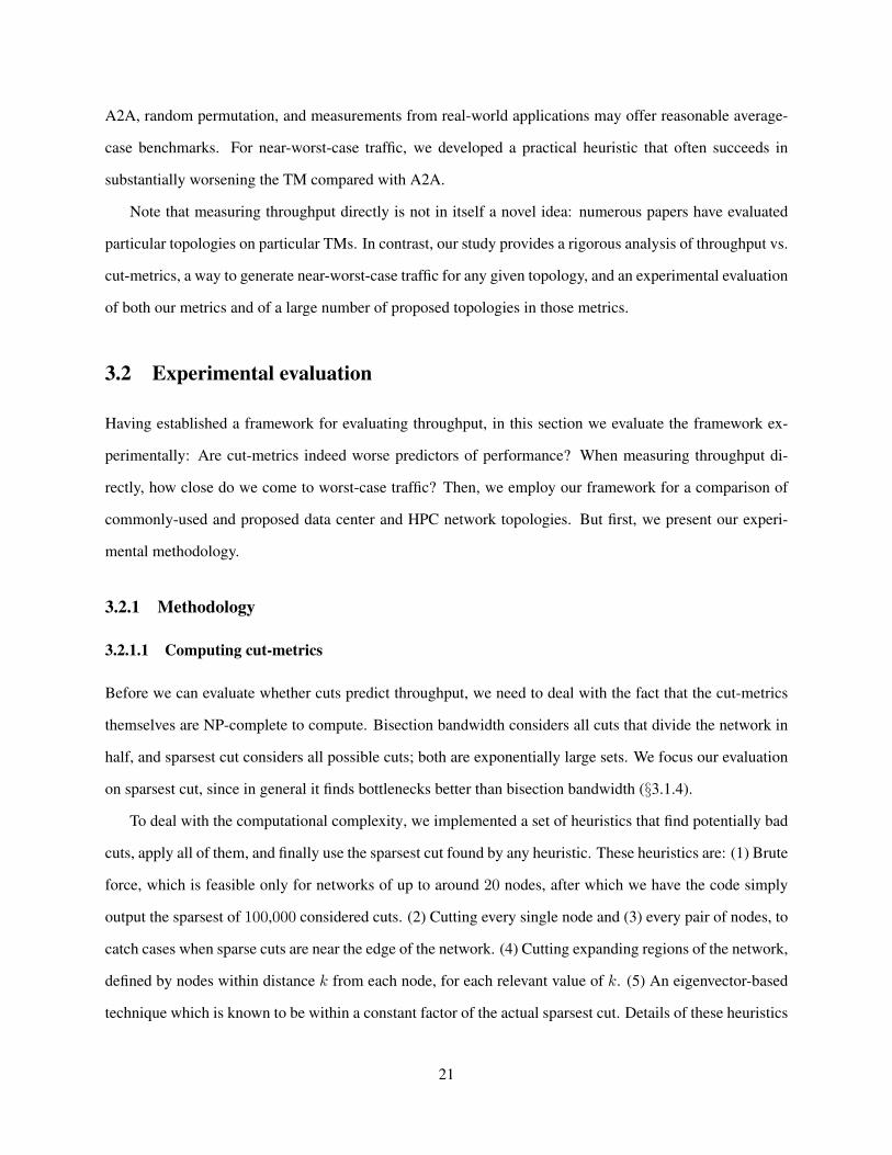
3.2.2.2 Can we find near-worst-case traffic?
In this section, we evaluate our proposed throughput metric — in particular, how closely the TMs of §3.1.7
approach the worst case. We compare representative samples from each family of network under four types
of TM: all to all (A2A), random matching with 5 servers per switch, random matching with 1 server per
switch, and longest matching.
Figure 3.4 shows the throughput values normalized so that the theoretical lower bound on throughput
is 1, and therefore A2A’s throughput is 2. For all networks, TA2A � TRM(5)
� TRM(1)
� TLM � 1,
matching the intuition discussed in §3.1.7. (As in Figure 3.3, throughput comparisons are valid across TMs
for a particular network, not across networks. The networks used in this plot support approximately 250
servers each. However, the exact number of switches, links and servers varies across networks.)
Our longest matching TM is successful in matching the lower bound for BCube, Hypercube, HyperX,
and (nearly) Dragonfly. In all other families except fat trees, the traffic under longest matching is signifi-
cantly closer to the lower bound than with the other TMs. In fat trees, throughput under A2A and longest
matching are equal. However, this is a characteristic of the network and not a shortcoming of the metric.
In fat trees, it can be easily verified that the normalized traffic is the same under all TMs. In short, these
results show that throughput measurement using longest matching is a more accurate estimate of worst-case
throughput performance than cut-based approximations, in addition to being substantially easier to compute.
26

0 0.2 0.4 0.6 0.8
1 1.2 1.4 1.6
100 1000 10000
Rel
. Thr
ough
put
Number of servers
BCubeDCell
Dragonfly
Fat treeFlattened BF
Hypercube
0 0.2 0.4 0.6 0.8
1 1.2 1.4 1.6
100 1000 10000
Rel
. Thr
ough
put
Number of servers
(a) All to All TM
0 0.2 0.4 0.6 0.8
1 1.2 1.4 1.6
100 1000 10000
Rel
. Thr
ough
put
Number of servers
(b) Random Matching TM
0 0.2 0.4 0.6 0.8
1 1.2 1.4 1.6
100 1000 10000
Rel
. Thr
ough
put
Number of servers
(c) Longest Matching TM
Figure 3.5 Comparison of TMs on topologies.
3.2.3 Evaluation of topologies
Although the longest matching TM can give near worst-case performance results with limited computational
effort, there is one more piece of the puzzle to allow comparison of networks. Networks may be built with
different equipment – with a wide variation in number of switches and links. The raw throughput value does
not account for this difference in network resources, and most proposed topologies can only be built with
particular discrete numbers of servers, switches, and links, which inconveniently do not match.
Fortunately, uniform-random graphs like our Jellyfish design (Chapter 4) can be constructed for any
size and specified degree distribution. Hence, random graphs serve as a convenient benchmark for easy
comparison of network topologies. Our high-level approach to evaluating a network is to: (i) compute the
network’s throughput; (ii) build a random graph with precisely the same equipment, i.e., the same number
of nodes each with the same number of links as the corresponding node in the original graph, (iii) compute
27

0 0.2 0.4 0.6 0.8
1 1.2 1.4 1.6
100 1000 10000
Rel
. Thr
ough
put
Number of servers
HyperXJellyfish
Long HopSlim Fly
0 0.2 0.4 0.6 0.8
1 1.2 1.4 1.6
100 1000 10000
Rel
. Thr
ough
put
Number of servers
(a) All to All TM
0 0.2 0.4 0.6 0.8
1 1.2 1.4 1.6
100 1000 10000
Rel
. Thr
ough
put
Number of servers
(b) Random Matching TM
0 0.2 0.4 0.6 0.8
1 1.2 1.4 1.6
100 1000 10000
Rel
. Thr
ough
put
Number of servers
(c) Longest Matching TM
Figure 3.6 Comparison of TMs on more topologies.
the throughput of this same-equipment random graph under the same TM; (iv) normalize the network’s
throughput with the random graph’s throughput for comparison against other networks. This normalized
value is referred to as relative throughput. Unless otherwise stated, each data-point is an average across
10 iterations, and all error bars are 95% two-sided confidence intervals. Minimal variations lead to narrow
error bars in networks of size greater than 100.
We evaluate the performance of 10 types of computer networks under all three traffic matrices: all to
all, random matching with one server, and longest matching. Figures 3.5 and 3.6 show the results, divided
among two figures for visual clarity. Most topologies are in Figure 3.5, while Figure 3.6 shows Jellyfish,
Slim Fly, Long Hop, and HyperX.
Overall, performance varies substantially, by around 1.6⇥ with A2A traffic and more than 2⇥ with longest
matching. Furthermore, for the networks of Figure 3.5, which topology “wins” depends on the TM. For
28

example, Dragonfly has high relative throughput under A2A but under the longest matching TM, fat trees
achieve the highest throughput at the largest scale. However, in all TMs, the Jellyfish random graph achieves
consistently highest performance (relative throughput = 1 by definition), with Long Hop matching that per-
formance at the largest scale. In comparison with random graphs, performance degrades for most networks
with increasing size. We discuss each network’s performance in detail below. Unless otherwise stated,
reported metrics correspond to the largest network tested in each family.
BCube [42] The 2-ary BCube achieves 73% of the random graph’s throughput under all to all traffic and
90% under random matching, but only 51% under longest matching.
DCell [43] 5-ary DCell achieves 93% of the random graph’s throughput under all to all, 97% under random
matching, and 79% under longest matching. The relative throughput performance degrades as the network
size increases.
Dragonfly [53] networks constructed with low-radix switches of degrees varying from 4 to 8 have through-
put performance under all-to-all traffic equal that of random graphs, i.e., a relative throughput approximately
equal to 1. However, the performance degrades to 76% under random matching and further down to 72%
under longest matching for the network constructed from switches of degree 8.
Fat Tree [7] constructed from switches of degree 14 can achieve only 65% of the throughput of random
graphs under A2A. Interestingly, a fat tree achieves 73% of a random graph’s throughput under random
matching, and 89% with longest matching. While the fat-tree’s non-blocking design is overkill for the
random matching, compared to networks other than the random graph, it is advantageous for the longest
matching. Note that the fat-tree’s absolute performance does not improve when moving to the more dif-
ficult longest matching TM; instead, its relative throughput is higher because longest matching degrades
performance more in the random graph than in the fat-tree.
Flattened butterfly [52] At the largest scale, the 2-ary flattened butterfly which can support 1024 servers
achieves only 59% of the random graph’s throughput under all-to-all traffic, but the performance improves
to 71% under random matching. However, the worst-case performance under longest matching drops to
47% which is the worst performance across all topologies tested.
Hypercubes [47] achieve 72% of the random graph’s throughput under all-to-all traffic, 84% under random
matching, and 51% under longest matching.
29

0 0.1 0.2 0.3 0.4 0.5 0.6 0.7 0.8 0.9
1
200 400 600 800 1000 1200
Rel
ativ
e T
hrou
ghpu
t
Number of servers
Bisection 0.2Bisection 0.4Bisection 0.5
Figure 3.7 HyperX relative throughput under longest matching with different bisection bandwidths.
0
0.2
0.4
0.6
0.8
1
1.2
100 1000 10000
Rel
ativ
e T
hrou
ghpu
t
Number of servers
Dimension 5 Dimension 6 Dimension 7
Figure 3.8 Long Hop relative throughput under longest matching TM.
0 0.2 0.4 0.6 0.8
1 1.2 1.4 1.6
100 1000 10000 0 0.2 0.4 0.6 0.8 1 1.2 1.4 1.6
Rel
ativ
e T
hrou
ghpu
t
Rel
ativ
e pa
th le
ngth
Number of servers
Rel. ThroughputRel. path length
Figure 3.9 Slim Fly relative throughput under longest matching TM.
30
HyperX [6] Unlike other topologies, the performance of HyperX is irregular. The variations arise from
the choice of underlying topology: Given switch radix, number of servers and desired bisection bandwidth,
HyperX attempts to find the least cost topology constructed from the building blocks – hypercube and
flattened butterfly. Even a slight variation in one of the parameters can lead to a significant difference in
HyperX construction and throughput.
We plot HyperX results for networks with bisection bandwidth of 0.4. In the worst case, the HyperX
network that can support 648 hosts achieves a relative throughput of 55% under all-to-all traffic. For the same
network, relative performance improves to 67% under random matching but further degrades to 45% under
longest matching. We investigate the performance of HyperX networks with different bisection bandwidths
under longest matching TM in Figure 3.7 and observe that the performance varies widely with network size
under all values of bisection. More importantly, this further illustrates that high bisection does not guarantee
high performance.
Jellyfish is our benchmark, and its (average) relative performance is 100% under all workloads by defini-
tion. Performance depends on randomness in the construction, but at larger sizes, performance differences
between Jellyfish instances are minimal (⇡ 1%).
Long Hop networks [82] In Figure 3.8, we show that the relative throughput of Long Hop networks ap-
proaches 1 at large sizes under the longest matching TM. Similar trends are observed under both all-to-all
and random matching workloads. The paper [82] claimed high performance (in terms of bisection band-
width) with substantially less equipment than past designs, but we find that while Long Hop networks do
have high performance, they are no better than random graphs, and sometimes worse.
Slim Fly [14] It was noted in [14] that Slim Fly’s key advantage is path length. We observe in Figure 3.9 that
the topology indeed has extremely short paths – about 85-90% relative to the random graph – but this does
not translate to higher throughput. Slim Fly’s performance is essentially identical to random graphs under
all-to-all and random matching TMs with a relative performance of 101% using both. Relative throughput
under the longest matching TM decreases with scale, dropping to 80% at the largest size tested. Hence,
throughput performance cannot be predicted solely based on the average path length.
31

3.3 Comparison with related work
The literature on network topology design is large and growing, with a number of designs having been
proposed in the past few years [7, 41, 42, 73, 43, 83, 36, 80, 29, 30]. However, each of these research
proposals only makes a comparison with one or two other past proposals, with no standard benchmarks for
the comparison. There has been no independent, rigorous evaluation of a large number of topologies.
Popa et. al. [76] assess 4 topologies to determine the one that incurs least expense while achieving a
target level of performance under a specific workload (all-to-all traffic). Their attempts to equalize perfor-
mance required careful calibration, and approximations still had to be made. Accounting for the different
costs of building different topologies is an inexact process. We sidestep that issue by using the random
graph as a normalizer: instead of attempting to match performance, for each topology, we build a random
graph with identical equipment, and then compare throughput performance of the topology with that of the
random graph. Thus the problem of massaging structured designs into roughly equivalent configurations is
alleviated. This also makes it easy for others to use our tools, and to test arbitrary workloads. Apart from
comparing topologies, our work also argues the superiority of flow-metrics to cuts.
Other work on comparing topologies is more focused on reliability and cuts in the topology [55]. Sev-
eral researchers have also used sparsest cut and bisection bandwidth as proxies for throughput performance.
Further, the usage of these two terms is not consistent across the literature. For instance, REWIRE [30]
explicitly optimizes its topology designs for high sparsest cut, although it refers to the standard sparsest
cut metric as bisection bandwidth. Tomic [82] builds topologies with the objective of maximizing bisec-
tion bandwidth (in a particular class of graphs). Webb et. al [85] use bisection bandwidth to pick virtual
topologies over the physical topology. An interesting point of note is that they consider all-to-all traffic
“a worst-case communication scenario”, while our results (Figure 3.4) show that other traffic patterns can
be significantly worse. PAST [81] tests 3 data center network proposals with the same sparsest cut (while
referring to it as bisection bandwidth). Although it is not stated, the authors presumably used approximate
methods because even approximating sparsest cut is believed to be NP-Hard [21]. While that does not im-
ply that it could not be efficiently computed for these particular graphs, to the best of our knowledge, no
sparsest-cut computation procedures are known for any of the networks tested in PAST. Further, PAST finds
that the throughput performance of topologies with the same sparsest cut is different in packet-level simula-
tions, raising questions about the usefulness of such a comparison; one must either build topologies of the
32

0
0.2
0.4
0.6
0.8
1
1.2
Abs
olut
e T
hrou
ghpu
t
Comparison 1:[Yuan]
Comparison 2:Opt. throughput
Comparison 3:Opt. throughput,same equipment
Fat tree Jellyfish
Figure 3.10 Throughput comparison of Fat-tree and Jellyfish based on [89], showing the effect of twomethodological changes.
same cost and compare them on throughput (as we do), or build topologies with the same performance and
compare cost (as Popa et. al [76] do). These observations underscore the community’s lack of clarity on
the relationship between bisection bandwidth, sparsest cut, and throughput. A significant component of our
work tackles this subject.
We note that throughput comparisons are a subtle exercise. Naive approaches can yield conclusions that
are off by a sizable margin, for instance leading [89] to conclude that fat trees perform better than or similar
to Jellyfish. We replicated the method of [89] using their LLSKR routing scheme, also finding similar
throughput using the A2A TM (Fig. 3.10, Comparison 1). Roughly speaking, their method splits flows
into sub-flows and routes them along certain paths according to LLSKR. It then estimates each subflow’s
throughput by counting and inverting the maximum number of intersecting subflows at a link along the
path. When we move to the LP-based exact computation while still adhering to the same LLSKR path
restrictions, we measure slightly higher throughput in fat trees and substantially higher in Jellyfish, now
30% greater than fat trees (Fig. 3.10, Comparison 2). This is even though we now maximize the minimum
flow, while [89] measured the average! A second issue with the comparison in [89] is that more servers are
added to Jellyfish than to fat tree — with 80 switches in each topology, their procedure would compare a fat
tree with 128 servers to a Jellyfish topology with 160 servers. Equalizing all equipment, as in our standard
comparison method, with 80 switches and 128 servers in both topologies, increases the performance gap to
65% (Comparison 3).
33

3.4 Conclusion
Although high throughput is a core goal of network design, measuring throughput is a subtle problem.
We have shown that one common way of measuring throughput, via bisection and sparsest cut, produces
inaccurate predictions of performance. We have put forward an improved benchmark for network capacity,
including a near-worst-case traffic matrix, and have used this metric to compare a large number of network
topologies, revealing new perspective on performance of several proposals. Particularly when designing
networks for environments where traffic patterns may be unknown or variable and performance requirements
are stringent, we believe evaluation under the near-worst-case longest matching TM will be useful.
Our findings also raise interesting directions for future work. First, our longest-matching traffic heuris-
tically produces near-worst case performance, but does not always match the lower bound. Is there an effi-
cient method to produce even-worse-case traffic for any given topology, or provably approximate it within
less than 2⇥ Second, we observed that low average path length does not guarantee high throughput. How
is throughput correlated with other fundamental graph properties? High correlations could suggest im-
provement in network design, while small correlation would further position throughput as an independent
topological property of interest.
Our topology benchmarking tools and the topology datasets are all freely available [5].
34

CHAPTER 4
Homogeneous topology design
Having established our method of evaluating network throughput, we return to the problem of designing
data center networks for high throughput. In this chapter, we look at the following formulation of the
network design problem:
Given N switches each with k ports, and S servers each with one port, with all ports having unit
capacity, how should these ports be wired together in order to maximize network throughput?
In this setting, all the switches are homogeneous, i.e., have the same line-speeds and number of ports.
Nevertheless, this problem, like many other network topology design problems is hard because of the
combinatorial explosion of the solution search space with the network size. Data center network de-
signers have thus focused either on adapting known graph structures such as Clos networks [59] and hy-
percubes [47], or suggesting new ones based on intuitions about structure and symmetry (for instance,
DCell [43] and BCube [42]). However, while numerous data center network architectures have recently
been proposed [83, 36, 87, 42, 43, 41, 73, 59, 79, 52, 6] to achieve high throughput, none of these designs
address two crucial problems:
• Incremental network expansion: how do we design high throughput networks that allow incremental
addition of servers and switches?
• The optimality gap: how far are we from optimal topology design?
In the following, we discuss these two problems and our approach to addressing them.
This chapter includes previously published results from Jellyfish: Networking Data Centers Randomly. Ankit Singla, Chi-YaoHong, Lucian Popa, P. Brighten Godfrey. USENIX NSDI, 2012. Section §4.3 also includes results from High Throughput DataCenter Topology Design. Ankit Singla, P. Brighten Godfrey, and Alexandra Kolla. USENIX NSDI, 2014.
35

Incremental network expansion
Incremental network expansion may be necessitated by growth of the user base, which requires more servers,
or by the deployment of more bandwidth-hungry applications. Expansion within a data center is possible
through either planned overprovisioning of space and power, or by upgrading old servers to a larger number
of more powerful but energy-efficient new servers. Planned expansion is a practical strategy to reduce
up-front capital expenditure [60].
Industry experience indicates that incremental expansion is important. Consider the growth of Face-
book’s data center server population from roughly 30,000 in Nov. 2009 to >60,000 by June 2010 [69].
While Facebook has added entirely new data center facilities, much of this growth involves incrementally
expanding existing facilities by “adding capacity on a daily basis” [68]. For instance, in 2012, Facebook
announced that it would double the size of its facility at Prineville, Oregon [35]. A 2011 survey [31] of
300 enterprises that run data centers of a variety of sizes found that 84% of firms would probably or def-
initely expand their data centers in 2012. Several industry products advertise incremental expandability of
the server pool, including SGI’s IceCube (marketed as “The Expandable Modular Data Center” [4]; expands
4 racks at a time) and HP’s EcoPod [49] (a “pay-as-you-grow” enabling technology [48]).
Do current high-bandwidth data center network proposals allow incremental growth? Consider the
fat-tree interconnect, as proposed in [59], as an illustrative example. The entire structure is completely
determined by the port-count of the switches available. This is limiting in at least two ways. First, it makes
the design space very coarse: full bisection bandwidth fat-trees can only be built at sizes 3456, 8192, 27648,
and 65536 corresponding to the commonly available port counts of 24, 32, 48, and 64
1. Second, even if
(for example) 50-port switches were available, the smallest “incremental” upgrade from the 48-port switch
fat-tree would add 3,602 servers and would require replacing every switch.
There are, of course, some workarounds. One can replace a switch with one of larger port count or over-
subscribe certain switches, but this makes capacity distribution constrained and uneven across the servers.
One could leave free ports for future network connections [43, 29] but this wastes investment until actual ex-
pansion. Thus, without compromises on bandwidth or cost, such topologies are not amenable to incremental
growth.
Since it seems that structure hinders incremental expansion, we propose the opposite: a random network1Other topologies have similar problems: a hypercube [15] allows only power-of-2 sizes, a de Bruijn-like construction [76]
allows only power-of-3 sizes, etc.
36

interconnect. The proposed interconnect, which we call Jellyfish, is a degree-bounded2 random graph
topology among top-of-rack (ToR) switches. The inherently sloppy nature of this design has the potential
to be significantly more flexible than past designs. Additional components—racks of servers or switches to
improve capacity—can be incorporated with a few random edge swaps. Jellyfish also allows construction
of arbitrary-size networks, unlike topologies discussed above which limit the network to very coarse design
points dictated by their structure.
Somewhat surprisingly, Jellyfish supports more servers than a fat-tree [59] built using the same network
equipment while providing at least as high per-server bandwidth, measured either via bisection bandwidth or
in throughput under a random-permutation traffic pattern. In addition, Jellyfish has lower mean path length,
and is resilient to failures and miswirings.
The optimality gap
While all of the past literature makes claims of higher network capacity compared to a few preceding de-
signs, there has been no notion of optimality in this work. The question of how far we may be from optimal
topology design has been left completely unaddressed.
Towards answering this question, in this work, we prove a simple upper bound on the throughput achiev-
able by any hypothetical network from the space of all possible solutions to the network design problem
proposed above. Further, we show that our random graph based Jellyfish design achieves throughput within
a few percent of optimal.
Key contributions
Our key contributions and conclusions are as follows:
• We propose Jellyfish, an incrementally-expandable, high-bandwidth data center interconnect based
on random graphs.
• We show that Jellyfish provides quantitatively easier incremental expansion than prior work on incre-
mental expansion in Clos networks [29], growing incrementally at only 40% of the expense of [29].2Degree-bounded means that the number of connections per node is limited, in this case by switch port-counts.
37

• We show that Jellyfish can support 25% more servers than a fat-tree while using the same switch
equipment and providing at least as high bandwidth. This advantage increases with network size and
switch port-count.
• Further, we prove an upper bound on the throughput achievable by any topology with identical
switches, and show that Jellyfish achieves throughput surprisingly close to this boundwithin a few
percent at the scale of a few thousand servers for random permutation traffic.
• We also propose degree-diameter optimal graphs [28] as topologies which sit in the small optimality
gap between Jellyfish and the upper bound. Although these not as flexible as Jellyfish, for settings
such as modular containerized data centers, these may be a good topology choice.
We acknowledge that a data center network like Jellyfish, that lacks regular structure is a somewhat radical
departure from traditional designs, and this presents several important challenges that must be addressed
for Jellyfish to be viable. Among these are routing (schemes depending on a structured topology are not
applicable), physical construction, and cabling layout. Our solutions to these problems are discussed in
detail in Chapter 6, but we summarize the results here:
• Despite its lack of regular structure, packet-level simulations show that Jellyfish’s bandwidth can be
effectively utilized via existing forwarding technologies that provide high path diversity. The above
listed ‘25% more servers’ result accounts for the minor routing inefficiency in Jellyfish.
• We discuss effective techniques to realize physical layout and cabling of Jellyfish. Naively cabling
Jellyfish may lead to higher cabling cost than other topologies, since its cables can be longer; but smart
cabling schemes we propose make cabling Jellyfish cheaper than fat-trees while preserving most of
its throughput advantage.
4.1 Jellyfish topology
Construction: The Jellyfish approach is to construct a random graph at the top-of-rack (ToR) switch layer.
Each ToR switch i has some number ki of ports, of which it uses ri to connect to other ToR switches, and
uses the remaining ki � ri ports for servers. In the simplest case, which we consider by default throughout
38

this chapter, every switch has the same number of ports and servers: 8i, k = ki and r = ri. With N racks,
the network supports N(k � r) servers. In this case, the network is a random regular graph, which we
denote as RRG(N , k, r). This is a well known construct in graph theory and has several desirable properties
as we shall discuss later.
Formally, RRGs are sampled uniformly from the space of all r-regular graphs. This is a complex prob-
lem in graph theory [63]; however, a simple procedure produces “sufficiently uniform” random graphs which
empirically have the desired performance properties. One can simply pick a random pair of switches with
free ports (for the switch-pairs are not already neighbors), join them with a link, and repeat until no further
links can be added. If a switch remains with � 2 free ports (p1
, p2
) — which includes the case of incremen-
tal expansion by adding a new switch — these can be incorporated by removing a uniform-random existing
link (x, y), and adding links (p1
, x) and (p2
, y). Thus only a single unmatched port might remain across the
whole network.
Using the above idea, we generate a blueprint for the physical interconnection. (Allowing human op-
erators to “wire at will” may result in poor topologies due to human biases – for instance, favoring shorter
cables over longer ones.) We discuss cabling later in §6.5.
Intuition: Our two key goals are high bandwidth and flexibility. The intuition for the latter property is
simple: lacking structure, the RRG’s network capacity becomes “fluid”, easily wiring up any number of
switches, heterogeneous degree distributions, and newly added switches with a few random link swaps.
But why should random graphs have high bandwidth? We show quantitative results later, but here we
present the intuition. The end-to-end throughput of a topology depends not only on the capacity of the
network, but is also inversely proportional to the amount of network capacity consumed to deliver each
byte — that is, the average path length. Therefore, assuming that the routing protocol is able to utilize the
network’s full capacity, and that there are no small cuts in the network (which is known from the good
expansion properties of random graphs [19]), low average path length allows us to support more flows at
high throughput. To see why Jellyfish has low path length, Fig. 4.1(a) and 4.1(b) visualize a fat-tree and a
representative Jellyfish topology, respectively, with identical equipment. Both topologies have diameter 6,
meaning that any server can reach all other servers in 6 hops. However, in the fat-tree, each server can only
reach 3 others in 5 hops. In contrast, in the random graph, the typical origin server labeled o can reach
12 servers in 5 hops, and 6 servers in 4 hops. The reason for this is that many edges in the fat-tree are
39

v
4
2
X
X
6
(a)
o
3
4
5 6
(b)
0 0.1 0.2 0.3 0.4 0.5 0.6 0.7 0.8 0.9
1
2 3 4 5 6
Frac
tion
of S
erve
r Pai
rs
Path length
Jellyfish Fat-tree
(c)
Figure 4.1 Random graphs have high throughput because they have low average path length, and therefore doless work to deliver each packet. (a): Fat-tree with 16 servers and 20 four-port switches. (b): Jellyfish with iden-tical equipment. The servers are leaf nodes; switches are interior nodes. Each ‘concentric’ ring contains serversreachable from any server v in the fat-tree, and an arbitrary server o in Jellyfish, within the number of hops in themarked label. Jellyfish can reach many more servers in few hops because in the fat tree, many edges (like thosemarked “X”) are redundant from a path-length perspective. (c): Path length distribution between servers for a686-server Jellyfish (drawn from 10 trials) and same-equipment fat-tree.
40

not useful from the perspective of their effect on path length; for example, deleting the two edges marked X
in Fig. 4.1(a) does not increase the path length between any pair of servers. In contrast, the RRG’s diverse
random connections lead to lower mean path length. Figure 4.1(c) demonstrates these effects at larger scale.
With 686 servers, >99.5% of source-destination pairs in Jellyfish can be reached in fewer than 6 hops, while
the corresponding number is only 7.5% in the fat-tree.
4.2 Jellyfish topology properties
This section evaluates the efficiency, flexibility and resilience of Jellyfish. Our goal is to measure the raw
capabilities of the topology, were they to be coupled with optimal routing and congestion control. We study
how to perform routing and congestion control separately, in Chapter 6. Further, while a comparison of 10
topologies is included in Chapter 3, we include herein detailed comparisons with the fat-tree, as well as a
related proposal based on a different random-graph model. Our key findings are:
• Jellyfish can support 27% more servers at full capacity than a (same-switching-equipment) fat-tree at
a scale of <900 servers. The trend is for this advantage to improve with scale.
• Jellyfish’s network capacity is >91% of the best-known degree-diameter graphs [28], which we pro-
pose as benchmark bandwidth-efficient graphs.
• Paths are shorter on average in Jellyfish than in a fat-tree, and the maximum shortest path length
(diameter) is the same or lower for all scales we tested.
• Incremental expansion of Jellyfish produces topologies identical in throughput and path length Jelly-
fish topologies generated from scratch.
• Jellyfish provides a significant cost-efficiency advantage over prior work (LEGUP [29]) on incremen-
tal network expansion in Clos networks. In a network expansion scenario that was made available
for us to test, Jellyfish builds a slightly higher-capacity expanded network at only 40% of LEGUP’s
expense.
• Jellyfish is highly failure resilient, even more so than the fat-tree. Failing a random 15% of all links
results in a capacity decrease of <16%.
41

Evaluation methodology: Some of the results for network capacity in this section are based on explicit
calculations of the theoretical bounds for bisection bandwidth for regular random graphs.
All throughput results presented in this section are based on calculations of throughput for a specific
class of traffic demand matrices with optimal routing. While the details and rationale of our throughput
metric are discussed in Chapter 3, we give a brief summary of methodology here.
The traffic matrices we use are random permutation traffic: each server sends at its full output link rate
to a single other server, and receives from a single other server, and this permutation is chosen uniform-
randomly. Intuitively, random permutation traffic represents the case of no locality in traffic, as might arise
if VMs are placed without regard to what is convenient for the network3. Nevertheless, evaluating other
traffic patterns is an important question that we leave for future work.
Given a traffic matrix, we characterize a topology’s raw capacity with “ideal” load balancing by treating
flows as splittable and fluid. This corresponds to solving a standard multi-commodity network flow problem,
using a linear program solver.
For all throughput comparisons, we use the same switching equipment (in terms of both number of
switches, and ports on each switch) for each set of topologies compared. Throughput results are always
normalized to [0, 1], and averaged over all flows.
For comparisons with the full bisection bandwidth fat-tree, we attempt to find, using a binary search
procedure, the maximum number of servers Jellyfish can support using the same switching equipment as the
fat-tree while satisfying the full traffic demands. Specifically, each step of the binary search checks a certain
number of servers m by sampling three random permutation traffic matrices, and checking whether Jellyfish
supports full capacity for all flows in all three matrices. If so, we say that Jellyfish supports m servers at
full capacity. After our binary search terminates, we verify that the returned number of servers is able to get
full capacity over each of 10 more samples of random permutation traffic matrices.
4.2.1 Efficiency
Bisection bandwidth vs. fat-tree: Bisection bandwidth, a common measure of network capacity, is the
worst-case bandwidth spanning any two equal-size partitions of a network. Here, we compute the fat-tree’s
bisection bandwidth directly from its parameters; for Jellyfish, we model the network as a RRG and apply3Supporting such flexible network-oblivious VM placement without a performance penalty is highly desirable [46].
42

0.2
0.4
0.6
0.8
1
1.2
1.4
1.6
0 10 20 30 40 50 60 70 80
Nor
mal
ized
Bis
ectio
n Ba
ndw
idth
Number of Servers in Thousands
Jellyfish; N=2880; k=48Fat-tree; N=2880; k=48Jellyfish; N=1280; k=32Fat-tree; N=1280; k=32Jellyfish; N=720; k=24Fat-tree; N=720; k=24
(a)
0
50
100
150
200
250
300
350
400
10 20 30 40 50 60 70 80
Equi
pmen
t Cos
t [#P
orts
in T
hous
ands
]
Number of Servers in Thousands
Increasing port-count
Fat-tree; {24,32,48,64} portsJellyfish; 24 portsJellyfish; 32 portsJellyfish; 48 portsJellyfish; 64 ports
(b)
0
100
200
300
400
500
600
700
800
900
0 500 1000 1500 2000 2500 3000 3500
#Ser
vers
at F
ull T
hrou
ghpu
t
Equipment Cost [Total #Ports] Using Identical Equipment
Jellyfish (Optimal routing)Fat-tree (Optimal routing)
(c)
Figure 4.2 Jellyfish offers virtually continuous design space, and packs in more servers at high network capacityat the same expense as a fat-tree. From theoretical bounds: (a) Normalized bisection bandwidth versus the numberof servers supported; equal-cost curves, and (b) Equipment cost versus the number of servers for commodity-switchport-counts (24, 32, 48) at full bisection bandwidth. Under optimal routing, with random-permutation traffic: (c)Servers supported at full capacity with the same switching equipment, for 6, 8, 10, 12 and 14-port switches. Resultsfor (c) are averaged over 8 runs.
a lower bound of Bollobas [16]. We normalize bisection bandwidth by dividing it by the total line-rate
bandwidth of the servers in one partition4.
Fig. 4.2(a) shows that at the same cost, Jellyfish supports a larger number of servers (x axis) at full
bisection bandwidth (y axis = 1). For instance, at the same cost as a fat-tree with 16,000 servers, Jellyfish
can support >20,000 servers at full bisection bandwidth. Also, Jellyfish allows the freedom to accept lower
bisection bandwidth in exchange for supporting more servers or cutting costs by using fewer switches.
Fig. 4.2(b) shows that the cost of building a full bisection-bandwidth network increases more slowly
with the number of servers for Jellyfish than for the fat-tree, especially for high port-counts. Also, the design
choices for Jellyfish are essentially continuous, while the fat-tree (following the design of [59]) allows only4Values larger than 1 indicate overprovisioning.
43

0 0.2 0.4 0.6 0.8 1Normalized Throughput
Jellyfish
Small World Ring
Small World 2D-Torus
Small World 3D-Hex-Torus
Figure 4.3 Jellyfish has higher capacity than the (same-equipment) small world data center topologies [79] builtusing a ring, a 2D-Torus, and a 3D-Hex-Torus as the underlying lattice. Results are averaged over 10 runs.
certain discrete jumps in size which are further restricted by the port-counts of available switches. (Note
that this observation would hold even for over-subscribed fat-trees.)
Jellyfish’s advantage increases with port-count, approaching twice the fat-tree’s bisection bandwidth.
To see this, note that the fat-tree built using k-port switches has k3/4 servers, and being a full-bisection
interconnect, it has k3/8 edges crossing each bisection. The fat-tree has k3/2 switch-switch links, implying
that its bisection bandwidth represents 1
4
of its switch-switch links. For Jellyfish, in expectation, 1
2
of its
switch-switch links cross any given bisection of the switches, which is twice that of the fat-tree assuming
they are built with the same number of switches and servers. Intuitively, Jellyfish’s worst-case bisection
should be slightly worse than this average bisection. The bound of [16] bears this out: in almost every
r-regular graph with N nodes, every set of N/2 nodes is joined by at least N(
r4
�
pr ln 2
2
) edges to the rest
of the graph. As the number of network ports r ! 1 this quantity approaches Nr/4, i.e., 1
2
of the Nr/2
links.
Throughput vs. fat-tree: Fig. 4.2(c) uses the random-permutation traffic model to find the number of
servers Jellyfish can support at full capacity, matching the fat-tree in capacity and switching equipment. The
improvement is as much as 27% more servers than the fat-tree at the largest size (874 servers) we are able
to evaluate. As with results from Bollobas’ theoretical lower bounds on bisection bandwidth (Fig. 4.2(a),
4.2(b)), the trend indicates that this improvement increases with scale.
Throughput vs. small world data centers (SWDC): SWDC [79] proposes a new topology for data centers
inspired by a small-world distribution. We compare Jellyfish with SWDC using the same degree-6 topolo-
gies described in the SWDC paper. We emulate their 6-interface server-based design by using switches
connected with 1 server and 6 network ports each. We build the three SWDC variants described in [79] at
topology sizes as close to each other as possible (constrained by the lattice structure underlying these topolo-
44
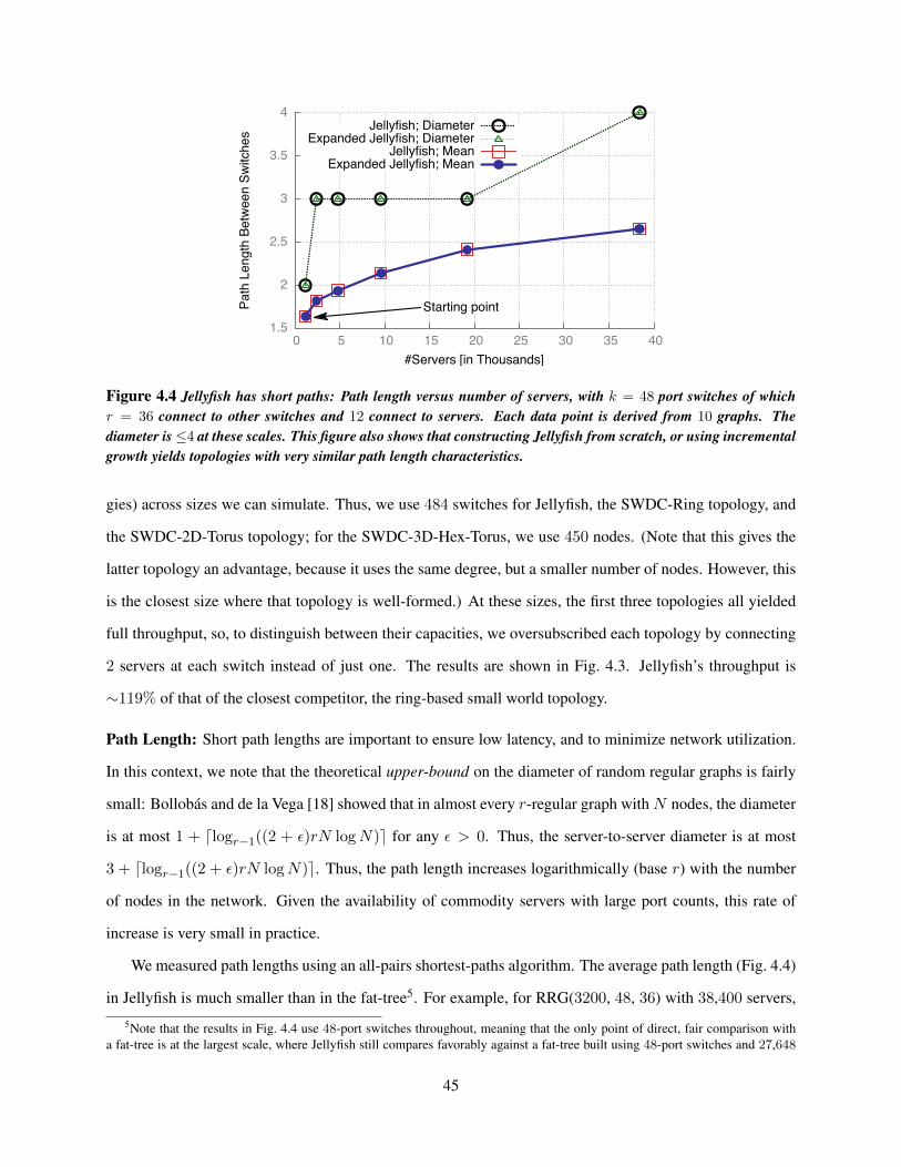
1.5
2
2.5
3
3.5
4
0 5 10 15 20 25 30 35 40
Path
Len
gth
Betw
een
Switc
hes
#Servers [in Thousands]
Starting point
Jellyfish; DiameterExpanded Jellyfish; Diameter
Jellyfish; MeanExpanded Jellyfish; Mean
Figure 4.4 Jellyfish has short paths: Path length versus number of servers, with k = 48 port switches of whichr = 36 connect to other switches and 12 connect to servers. Each data point is derived from 10 graphs. Thediameter is 4 at these scales. This figure also shows that constructing Jellyfish from scratch, or using incrementalgrowth yields topologies with very similar path length characteristics.
gies) across sizes we can simulate. Thus, we use 484 switches for Jellyfish, the SWDC-Ring topology, and
the SWDC-2D-Torus topology; for the SWDC-3D-Hex-Torus, we use 450 nodes. (Note that this gives the
latter topology an advantage, because it uses the same degree, but a smaller number of nodes. However, this
is the closest size where that topology is well-formed.) At these sizes, the first three topologies all yielded
full throughput, so, to distinguish between their capacities, we oversubscribed each topology by connecting
2 servers at each switch instead of just one. The results are shown in Fig. 4.3. Jellyfish’s throughput is
⇠119% of that of the closest competitor, the ring-based small world topology.
Path Length: Short path lengths are important to ensure low latency, and to minimize network utilization.
In this context, we note that the theoretical upper-bound on the diameter of random regular graphs is fairly
small: Bollobas and de la Vega [18] showed that in almost every r-regular graph with N nodes, the diameter
is at most 1 + dlogr�1
((2 + ✏)rN logN)e for any ✏ > 0. Thus, the server-to-server diameter is at most
3 + dlogr�1
((2 + ✏)rN logN)e. Thus, the path length increases logarithmically (base r) with the number
of nodes in the network. Given the availability of commodity servers with large port counts, this rate of
increase is very small in practice.
We measured path lengths using an all-pairs shortest-paths algorithm. The average path length (Fig. 4.4)
in Jellyfish is much smaller than in the fat-tree5. For example, for RRG(3200, 48, 36) with 38,400 servers,5Note that the results in Fig. 4.4 use 48-port switches throughout, meaning that the only point of direct, fair comparison with
a fat-tree is at the largest scale, where Jellyfish still compares favorably against a fat-tree built using 48-port switches and 27,648
45

the average path length between switches is <2.7 (Fig. 4.4), while the fat-tree’s average is 3.71 at the
smallest size, 3.96 at the size of 27,648 servers. Even though Jellyfish’s diameter is 4 at the largest scale,
the 99.99th percentile path-length across 10 runs did not exceed 3 for any size in Fig. 4.4.
4.2.2 Flexibility
Arbitrary-sized Networks: Several existing proposals admit only the construction of interconnects with
very coarse parameters. For instance, a 3-level fat-tree allows only k3/4 servers with k being restricted
to the port-count of available switches, unless some ports are left unused. This is an arbitrary constraint,
extraneous to operational requirements. In contrast, Jellyfish permits any number of racks to be networked
efficiently.
Incremental Expandability: Jellyfish’s construction makes it amenable to incremental expansion by adding
either servers and/or network capacity (if not full-bisection bandwidth already), with increments as small as
one rack or one switch. Jellyfish can be expanded such that rewiring is limited to the number of ports being
added to the network; and the desirable properties are maintained: high bandwidth and short paths at low
cost.
As an example, consider an expansion from an RRG(N , k, r) topology to RRG(N + 1, k, r). In other
words, we are adding one rack of servers, with its ToR switch u, to the existing network. We pick a random
link (v, w) such that this new ToR switch is not already connected with either v or w, remove it, and add
the two links (u, v) and (u,w), thus using 2 ports on u. This process is repeated until all ports are filled (or
a single odd port remains, which could be matched with another free port on an existing rack, used for a
server, or left free). This completes incorporation of the rack, and can be repeated for as many new racks as
desired.
A similar procedure can be used to expand network capacity for an under-provisioned Jellyfish network.
In this case, instead of adding a rack with servers, we only add the switch, connecting all its ports to the
network.
Jellyfish also allows for heterogeneous expansion: nothing in the procedure above requires that the
new switches have the same number of ports as the existing switches. Thus, as new switches with higher
port-counts become available, they can be readily used, either in racks or to augment the interconnect’s
servers.
46

0.7
0.75
0.8
0.85
0.9
0.95
1
0 100 200 300 400 500 600 700
Nor
mal
ized
Thr
ough
put
#Servers
Jellyfish (Incremental)Jellyfish (From Scratch)
Figure 4.5 Incrementally constructed Jellyfish has the same capacity as Jellyfish built from scratch: We built aJellyfish topology incrementally from 20 to 160 switches in increments of 20 switches, and compared the throughputper server of these incrementally grown topologies to Jellyfish topologies built from scratch using our constructionroutine. The plot shows the average, minimum and maximum throughput over 20 runs.
bandwidth. There is, of course, the possibility of taking into account heterogeneity explicitly in the random
graph construction and to improve upon what the vanilla random graph model yields. This (among other
related problems) is addressed in Chapter 5.
We note that our expansion procedures (like our construction procedure) may not produce uniform-
random RRGs. However, we demonstrate that the path length and capacity measurements of topologies
we build incrementally match closely with ones constructed from scratch. Fig. 4.4 shows this comparison
for the average path length and diameter where we start with an RRG with 1,200 servers and expand it
incrementally. Fig. 4.5 compares the normalized throughput per server under a random permutation traffic
model for topologies built incrementally against those built from scratch. The incremental topologies here
are built by adding successive increments of 20 switches, and 80 servers to an initial topology also with 20
switches and 80 servers. (Throughout this experiment, each switch has 12 ports, 4 of which are attached to
servers.) In each case, the results are close to identical.
Network capacity under expansion: Note that after normalizing by the number of servers N(k � r), the
lower bound on Jellyfish’s normalized bisection bandwidth (§4.2.1) is independent of network size N . Of
course, as N increases with fixed network degree r, average path length increases, and therefore, the demand
for additional per-server capacity increases6. But since path length increases very slowly (as discussed6This discussion also serves as a reminder that bisection-bandwidth, while a good metric of network capacity, is not the same
as, say, capacity under worst-case traffic patterns.
47

0
0.2
0.4
0.6
0.8
1
2 3 4 5 6 7 8 9 10
Nor
mal
ized
Bis
ectio
n Ba
ndw
idth
Total Budget [in $100,000]
Increasing cost
JellyfishLEGUP
Figure 4.6 Jellyfish’s incremental expansion is substantially more cost-effective than LEGUP’s Clos network ex-pansion. With the same budget for equipment and rewiring at each expansion stage (x-axis), Jellyfish obtainssignificantly higher bisection bandwidth (y-axis). Results are averaged over 10 runs. (The drop in Jellyfish’s bisec-tion bandwidth from stage 0 to 1 occurs because the number of servers increases in that step.)
above), bandwidth per server remains high even for relatively large factors of growth. Thus, operators can
keep the servers-per-switch ratio constant even under large expansion, with minor bandwidth loss. Adding
only switches (without servers) is another avenue for expansion which can preserve or even increase network
capacity. Our below comparison with LEGUP uses both forms of expansion.
Comparison with LEGUP [29]: While a LEGUP implementation is not publicly available, the authors
were kind enough to supply a series of topologies produced by LEGUP. In this expansion arc, there is
a budget constraint for the initial network, and for each successive expansion step; within the constraint,
LEGUP attempts to maximize network bandwidth, and also may keep some ports free in order to ease
expansion in future steps. The initial network is built with 480 servers and 34 switches; the first expansion
adds 240 more servers and some switches; and each remaining expansion adds only switches. To build a
comparable Jellyfish network, at each expansion step, under the same budget constraints, (using the same
cost model for switches, cabling, and rewiring) we buy and randomly cable in as many new switches as we
can. The number of servers supported is the same as LEGUP at each stage.
LEGUP optimizes for bisection bandwidth, so we compare both LEGUP and Jellyfish on that metric
(using code provided by the LEGUP authors [29]) rather than on our previous random permutation through-
put metric. The results are shown in Fig. 4.6. Jellyfish obtains substantially higher bisection bandwidth than
LEGUP at each stage. In fact, by stage 2, Jellyfish has achieved higher bisection bandwidth than LEGUP in
48

0.6
0.65
0.7
0.75
0.8
0.85
0.9
0.95
1
0 0.05 0.1 0.15 0.2 0.25
Nor
mal
ized
Thr
ough
put
Fraction of Links Failed Randomly
Jellyfish (544 Servers)Fat-tree (432 Servers)
Figure 4.7 Jellyfish is highly resilient to failures: Normalized throughput per server decreases more gracefully forJellyfish than for a same-equipment fat-tree as the percentage of failed links increases. Note that the y-axis startsat 60% throughput; both topologies are highly resilient to failures.
stage 8, meaning (based on each stage’s cost) that Jellyfish builds an equivalent network at cost 60% lower
than LEGUP.
A minority of these savings is explained by the fact that Jellyfish is more bandwidth-efficient than Clos
networks, as exhibited by our earlier comparison with fat-trees. But in addition, LEGUP appears to pay
a significant cost to enable it to incrementally-expand a Clos topology; for example, it leaves some ports
unused in order to ease expansion in later stages. We conjecture that to some extent, this greater incremental
expansion cost is fundamental to Clos topologies.
4.2.3 Failure resilience
Jellyfish provides good path redundancy; in particular, an r-regular random graph is almost surely r-
connected [17]. Also, the random topology maintains its (lack of) structure in the face of link or node
failures – a random graph topology with a few failures is just another random graph topology of slightly
smaller size, with a few unmatched ports on some switches.
Fig. 4.7 shows that the Jellyfish topology is even more resilient than the same-equipment fat-tree (which
itself is no weakling). Note that the comparison features a fat-tree with fewer servers, but the same cost.
This is to justify Jellyfish’s claim of supporting a larger number of servers using the same equipment as the
fat-tree, in terms of capacity, path length, and resilience simultaneously.
49

4.3 Near-optimality of Jellyfish
We refer the reader again to the network design problem which is the subject of this chapter:
Given N switches each with k ports, and S servers each with one port, with all ports having unit
capacity, how should these ports be wired together in order to maximize throughput?
Jellyfish, fat-trees, and other topologies are merely points in the combinatorically large design space
of all graphs that address the above problem. While Jellyfish achieves higher throughput than the fat-tree,
could some other topology achieve much higher throughput than Jellyfish itself?
We begin by noting that the symmetry of the problem suggests that each switch be connected to the same
number of servers. Intuitively, spreading servers across switches in a manner that deviates from uniformity
will create bottlenecks at the switches with larger numbers of servers. Thus, we assume that each switch
uses out of its k ports, r ports to connect to other switches, and k � r ports for servers. For simplicity, we
also assume S = N ⇤ (k � r). Now we can limit our focus to the switch-switch interconnect.
The design space for such networks is the set of all subgraphs H of the complete graph over N nodes
KN , such that H has degree r. For generic, application-oblivious design, we assume that the objective is to
maximize throughput under a uniform traffic matrix such as all-to-all traffic or random permutation traffic
among servers. To account for fairness, the network’s throughput is defined as the maximum value of the
minimum flow between source-destination pairs. We denote such a throughput measurement of an r-regular
subgraph H of KN under uniform traffic with f flows by TH(N, r, f). (For more details on the throughput
metric, please refer back to Chapter 3.) The average path length of the network is denoted by hDi.
For this scenario, we prove a simple upper bound on the throughput achievable by any hypothetical
network.
Theorem 3. TH(N, r, f) NrhDif .
Proof. The network has a total of Nr edges (counting both directions) of unit capacity, for a total capacity of
Nr. A flow i whose end points are a shortest path distance di apart, consumes at least xidi units of capacity
in to obtain throughput xi. Thus, the total capacity consumed by all flows is at leastX
i
xidi. Given that
we defined network throughput TH(N, r, f) as the minimum flow throughput, 8i, xi � TH(N, r, f). Total
50

0
0.2
0.4
0.6
0.8
1
0 5 10 15 20 25 30 35
Thr
ough
put
(Rat
io t
o U
pper
-bou
nd)
Network Degree
All to AllPermutation (10 Servers per switch)Permutation (5 Servers per switch)
(a)
1
1.5
2
2.5
3
3.5
4
0 5 10 15 20 25 30 35
Path
Len
gth
Network Degree
Observed ASPLASPL lower-bound
(b)
Figure 4.8 Random graphs versus the bounds: (a) Throughput and (b) average shortest path length (ASPL) inrandom regular graphs compared to the respective upper and lower bounds for any graph of the same size anddegree. The number of switches is fixed to 40 throughout. The network becomes denser rightward on the x-axis asthe degree increases.
capacity consumed is then at least TH(N, r, f)X
i
di. For uniform traffic patterns such as random permuta-
tions and all-to-all traffic,X
i
di = hDif because the average source-destination distance is the same as the
graph’s average shortest path distance. Also, total capacity consumed cannot exceed the network’s capacity.
Therefore, hDifTH(N, r, f) Nr, rearranging which yields the result.
Further, [20] proves a lower bound on the average shortest path length of any r-regular network of size
N :
hDi � d⇤ =
k�1X
j=1
jr(r � 1)
j�1
+ kR
N � 1
where R = N � 1�
k�1X
j=1
r(r � 1)
j�1
� 0
and k is the largest integer such that the inequality holds.
This result, together with Theorem 3, yields an upper bound on throughput: TH(N, r, f) Nrfd⇤ . Next,
we show experimentally that random regular graphs achieve throughput close to this bound.
A random regular graph, denoted as RRG(N , k, r), is a graph sampled uniform-randomly from the
space of all r-regular graphs of size N . This is a well-known construct in graph theory, on which Jellyfish
is based.
51

0
0.2
0.4
0.6
0.8
1
0 20 40 60 80 100 120 140 160 180 200
Thr
ough
put
(Rat
io t
o U
pper
-bou
nd)
Network Size
All to AllPermutation (10 Servers per switch)Permutation (5 Servers per switch)
(a)
1.2
1.4
1.6
1.8
2
2.2
2.4
2.6
0 20 40 60 80 100 120 140 160 180 200
Path
Len
gth
Network Size
Observed ASPLASPL lower-bound
(b)
Figure 4.9 Random graphs versus the bounds: (a) Throughput and (b) average shortest path length (ASPL) inrandom regular graphs compared to the respective upper and lower bounds for any graph of the same size anddegree. The degree is fixed to 10 throughout. The network becomes sparser rightward on the x-axis as the numberof nodes increases.
Fig. 4.8(a) and Fig. 4.9(a) compare throughput achieved by RRGs to the upper bound on throughput for
any topology built with the same equipment. Fig. 4.8(a) shows this comparison for networks of increasing
density (i.e., the degree r increases, while the number of nodes N remains fixed at 40) for 3 uniform traffic
matrices: a random permutation among servers with 5 servers at each switch, another with 10 servers at each
switch, and an all-to-all traffic matrix. For the high-density traffic pattern, i.e., all-to-all traffic, exact optimal
throughput is achieved by the random graph for degree r � 13. Fig. 4.9(a) shows a similar comparison for
increasing size N , with r = 10. Our simulator does not scale for all-to-all traffic because the number of
commodities in the flow problem increases as the square of the network size for this pattern. Fig. 4.8(b)
and 4.9(b) compare average shortest path length in RRGs to its lower bound. For both large network sizes,
and very high network density, RRGs are surprisingly close to the bounds (right side of both figures).
The curve in Fig. 4.9(b) has two interesting features. First, there is a “curved step” behavior, with
the first step at network size up to N = 101, and the second step beginning thereafter. To see why this
occurs, observe that the bound uses a tree-view of distances from any node — for a network with degree
d, d nodes are assumed to be at distance 1, d(d � 1) at distance 2, d(d � 1)
2 at distance 3, etc. While
this structure minimizes path lengths, it is optimistic — in general, not all edges from nodes at distance k
can lead outward to unique new nodes7. As the number of nodes N increases, at some point the lowest
level of this hypothetical tree becomes full, and a new level begins. These new nodes are more distant, so7In fact, prior work shows that graphs with this structure do not exist for d � 3 and diameter D � 3 [67].
52

1
2
3
4
5
6
17 53 161 485 1457 1
1.04
1.08
1.12
1.16
1.2
Path
Len
gth
Rat
io (
obse
rved
/ bo
und)
Network Size (log scale)
Observed ASPLASPL lower-bound
Ratio
Figure 4.10 ASPL in random graphs compared to the lower bound. The degree is fixed to 4 throughout. Thebound shows a “curved step” behavior. In addition, as the network size increases, the ratio of observed ASPL to thelower bound approaches 1. The x-tics correspond to the points where the bound begins new distance levels.
average path length suddenly increases more rapidly, corresponding to a new “step” in the bound. A second
feature is that as N ! 1, the ratio of observed ASPL to the lower bound approaches 1. This can be shown
analytically by dividing an upper bound on the random regular graph’s diameter [18] (which also upper-
bounds its ASPL) by the lower bound of [20]. For greater clarity, we show in Fig. 4.10 similar behavior for
degree d = 4, which makes it easier to show many “steps”.
4.3.1 Topologies with higher throughput than Jellyfish?
As we show above, Jellyfish achieves throughput close to optimal. Even so, are there topologies that achieve
throughput higher than Jellyfish, and closer still to the upper bound? Towards answering this question, we
compare Jellyfish’s capacity with that of the best known degree-diameter graphs. Below, we briefly explain
what these graphs are, and why this comparison is interesting.
There is a fundamental trade-off between the degree and diameter of a graph of a fixed vertex-set (say
of size N ). At one extreme is a clique — maximum possible degree (N � 1), and minimum possible
diameter (1). At the other extreme is a disconnected graph with degree 0 and diameter 1. The problem
of constructing a graph with maximum possible number N of nodes while preserving given diameter and
degree bounds is known as the degree-diameter problem and has received significant attention in graph
theory. The problem is quite difficult and the optimal graphs are only known for very small sizes: the largest
degree-diameter graph known to be optimal has N = 50 nodes, with degree 7 and diameter 2 [28]. A
53

0 0.2 0.4 0.6 0.8
1
(132, 4, 3)
(72, 7, 5)
(98, 6, 4)
(50, 11, 7)
(111, 8, 6)
(212, 7, 5)
(168, 10, 7)
(104, 16, 11)
(198, 24, 16)
Nor
mal
ized
Thr
ough
put
Best-known Degree-Diameter GraphJellyfish
Figure 4.11 Jellyfish’s network capacity is close to (i.e., ⇠91% or more in each case) that of the best-known degree-diameter graphs. The x-axis label (A, B, C) represents the number of switches (A), the switch port-count (B), andthe network degree (C). Throughput is normalized against the non-blocking throughput. Results are averaged over10 runs.
collection of optimal and best known graphs for other degree-diameter combinations is maintained at [28].
The degree-diameter problem relates to our objective in that short average path lengths imply low re-
source usage and thus high network capacity. Intuitively, the best known degree-diameter topologies should
support a large number of servers with high network bandwidth and low cost (small degree). While we
note the distinction between average path length (which relates more closely to the network capacity) and
diameter, degree-diameter graphs will have small average path lengths too.
Thus, we propose the best-known degree-diameter graphs as a benchmark for comparison. Note that
such graphs do not meet our incremental expansion objectives; we merely use them as a capacity benchmark
for Jellyfish topologies. But these graphs (and our measurements of them) may be of independent interest
since they could be deployed as highly efficient topologies in a setting where incremental upgrades are
unnecessary, such as a pre-fab container-based data center.
For our comparisons with the best-known degree-diameter graphs, the number of servers we attach to
the switches was decided such that full-bisection bandwidth was not hit for the degree-diameter graphs (thus
ensuring that we are measuring the full capacity of degree-diameter graphs.) Our results, in Fig. 4.11, show
that the best-known degree-diameter graphs do achieve higher throughput than Jellyfish, and thus improve
even more over fat-trees. But in the worst of these comparisons, Jellyfish still achieves ⇠91% of the degree-
diameter graph’s throughput.
54

4.4 Conclusion
We argue that Jellyfish is a highly flexible architecture for data center networks. It represents a novel
approach to the significant problems of incremental expansion, while enabling high capacity, short paths,
and resilience to failures and miswirings. Not only does Jellyfish achieve higher throughput than fat-trees
and other topologies, it achieves throughput within a few percent of optimal.
55

CHAPTER 5
Heterogeneous topology design
As discussed in Chapter 4, while the network topology design problem is hard, for the homogeneous case,
Jellyfish provides a flexible solution with nearly-optimal throughput. However, the case of heterogeneous
networks, i.e., networks composed of switches or servers with disparate capabilities, introduces even greater
complexity. Heterogeneous network equipment is, in fact, the common case in the typical data center:
servers connect to top-of-rack (ToR) switches, which connect to aggregation switches, which connect to
core switches, with each type of switch possibly having a different number of ports as well some variations
in line-speed. For instance, the ToRs may have both 1 Gbps and 10 Gbps connections while the rest of
the network may have only 10 Gbps links. Further, as the network expands over the years and new, more
powerful equipment is added to the data center, one can expect more heterogeneity — each year the number
of ports supported by non-blocking commodity Ethernet switches increases. While line-speed changes are
slower, the move to 10 Gbps and even 40 Gbps is happening now, and higher line-speeds are expected in the
near future.
In spite of heterogeneity being commonplace in data center networks, very little is known about hetero-
geneous network design. For instance, there is no clarity on whether the traditional ToR-aggregation-core
organization is superior to a “flatter” network without such a switch hierarchy; or on whether powerful core
switches should be connected densely together, or spread more evenly throughout the network.
To attack this problem, we use random graphs as building blocks for heterogeneous network design
by first optimizing the volume of connectivity between groups of nodes, and then forming connections
randomly within these volume constraints. Using this approach we obtain the following results:
• We show empirically that in this framework, for a set of switches with different port counts but uni-
This chapter includes previously published results from High Throughput Data Center Topology Design. Ankit Singla, P.Brighten Godfrey, and Alexandra Kolla. USENIX NSDI, 2014.
56

form line-speed, attaching servers to switches in proportion to the switch port count is optimal.
• In our investigation of networks built with two switch types (with different port-counts, but the same
line-speeds), somewhat surprisingly, we find that a wide range of connectivity arrangements provides
nearly identical throughput. A useful consequence of this result is that there is significant opportu-
nity for clustering switches to achieve shorter cable lengths on average, without compromising on
throughput. This is a result we will employ in developing our cabling scheme in Chapter 6.
• In the case of multiple line-speeds, we show that complex bottleneck behavior may appear and there
may be multiple configurations of equally high capacity.
• We apply the above insights to improving a real-world heterogeneous design. The topology proposed
in VL2 [41] incorporates heterogeneous line-speeds and port-counts, and has been deployed in Mi-
crosoft’s cloud data centers1. Using our approach, VL2’s throughput can be improved by as much
as 43% at the scale of a few thousand servers simply by rewiring existing equipment, with gains
increasing with network size.
While our results in Chapter 4 show that random graphs achieve close to the best possible throughput in
the homogeneous network design setting, we are unable, at present, to make a similar claim for heteroge-
neous networks, where node degrees and line-speeds may be different. However, in this chapter, we present
for this setting, interesting experimental results which challenge traditional topology design assumptions.
5.1 Simulation methodology
While the details of our throughput evaluation method have been discussed in Chapter 3, we summarize the
approach briefly here.
Our experiments measure the capacity of network topologies. For this chapter, our goal is to study
topologies explicitly independent of systems-level issues such as routing and congestion control. Thus, we
model network traffic using fluid splittable flows which are routed optimally. Throughput is then the solu-
tion to the standard maximum concurrent multi-commodity flow problem [58]. Note that by maximizing1Based on personal exchange, and mentioned at http://research.microsoft.com/en-us/um/people/
sudipta/.
57

0
0.2
0.4
0.6
0.8
1
0.4 0.6 0.8 1 1.2 1.4 1.6 1.8 2 2.2 2.4
Nor
mal
ized
Thr
ough
put
Number of Servers at Large Switches(Ratio to Expected Under Random Distribution)
3:1 Port-ratio2:1 Port-ratio3:2 Port-ratio
(a)
0
0.2
0.4
0.6
0.8
1
0.4 0.6 0.8 1 1.2 1.4 1.6 1.8 2 2.2 2.4
Nor
mal
ized
Thr
ough
put
Number of Servers at Large Switches(Ratio to Expected Under Random Distribution)
20 Small Switches30 Small Switches40 Small Switches
(b)
0
0.2
0.4
0.6
0.8
1
0.4 0.6 0.8 1 1.2 1.4 1.6 1.8 2 2.2 2.4
Nor
mal
ized
Thr
ough
put
Number of Servers at Large Switches(Ratio to Expected Under Random Distribution)
480 Servers510 Servers540 Servers
(c)
Figure 5.1 Distributing servers across switches: Peak throughput is achieved when servers are distributed propor-tionally to port counts i.e., x-axis=1, regardless of (a) the absolute port counts of switches; (b) the absolute countsof switches of each type; and (c) oversubscription in the network.
the minimum flow throughput, this model incorporates a strict definition of fairness. We use a linear pro-
gram solver to obtain the maximum flow. Unless otherwise specified, the workload we use is a random
permutation traffic matrix, where each server sends traffic to (and receives traffic from) exactly one other
server.
Any comparisons between networks are made using identical switching equipment, unless noted other-
wise. Across all experiments, we test a wide range of parameters, varying the network size, node degree,
and oversubscription. A representative sample of results is included here. Most experiments average results
across 20 runs, with standard deviations in throughput being ⇠1% of the mean except at small values of
throughput in the uninteresting cases. Exceptions are noted in the text.
58

5.2 Heterogeneous port counts
We consider a simple scenario where the network is composed of two types of switches with different port
counts (line-speeds being uniform throughout). Two natural questions arise that we shall explore here: (a)
How should we distribute servers across the two switch types to maximize throughput? (b) Does biasing the
topology in favor of more connectivity between larger switches increase throughput?
First, we shall assume that the interconnection is an unbiased random graph built over the remaining
connectivity at the switches after we distribute the servers. Later, we shall fix the server distribution but bias
the random graph’s construction. Finally we will examine the combined effect of varying both parameters
at once.
Distributing servers across switches: We vary the numbers of servers apportioned to large and small
switches, while keeping the total number of servers and switches the same2. We then build a random
graph over the ports that remain unused after attaching the servers. We repeat this exercise for several
parameter settings, varying the numbers of switches, ports, and servers. A representative sample of results
is shown in Fig. 5.1. The particular configuration in Fig. 5.1(a) uses 20 larger and 40 smaller switches,
with the port counts for the three curves in the figure being 30 and 10 (3:1), 30 and 15 (2:1), and 30 and
20 (3:2) respectively. Fig. 5.1(b) uses 20 larger switches (30 ports) and 20, 30 and 40 smaller switches
(20 ports) respectively for its three curves. Fig. 5.1(c) uses the same switching equipment throughout: 20
larger switches (30 ports) and 30 smaller switches (20 ports), with 480, 510, and 540 servers attached to the
network. Along the x-axis in each figure, the number of servers apportioned to the larger switches increases.
The x-axis label normalizes this number to the expected number of servers that would be apportioned to large
switches if servers were spread randomly across all the ports in the network. As the results show, distributing
servers in proportion to switch degrees (i.e., x-axis= 1) is optimal.
This result, while simple, is remarkable in the light of current topology design practices, where top-of-
rack switches are the only ones connected directly to servers.
Next, we conduct an experiment with a diverse set of switch types, rather than just two. We use a set of
switches such that their port-counts ki follow a power law distribution. We attach servers at each switch i in
proportion to k�i , using the remaining ports for the network. The total number of servers is kept constant as
we test various values of �. (Appropriate distribution of servers is applied by rounding where necessary to2Clearly, across the same type of switches, a non-uniform server-distribution will cause bottlenecks and sub-optimal throughput.
59

0.5 0.6 0.7 0.8 0.9
1 1.1 1.2 1.3
0 0.2 0.4 0.6 0.8 1 1.2 1.4 1.6
Nor
mal
ized
Thr
ough
put
β
Avg port-count 6Avg port-count 8
Avg port-count 10
Figure 5.2 Distributing servers across switches: Switches have port-counts distributed in a power-law distribution.Servers are distributed in proportion to the �th power of switch port-count. Distributing servers in proportion todegree (� = 1) is still among the optimal configurations.
achieve this.) � = 0 implies that each switch gets the same number of servers regardless of port count, while
� = 1 is the same as port-count-proportional distribution, which was optimal in the previous experiment.
The results are shown in Fig. 5.2. � = 1 is optimal (within the variance in our data), but so are other values
of � such as 1.2 and 1.4. The variation in throughput is large at both extremes of the plot, with the standard
deviation being as much as 10% of the mean, while for � 2 {1, 1.2, 1.4} it is < 4%.
Switch interconnection: We repeat experiments similar to the above, but instead of using a uniform ran-
dom network construction, we vary the number of connections across the two clusters of (large and small)
switches3. The distribution of servers is fixed throughout to be in proportion to the port counts of the
switches.
As Fig. 5.3 shows, throughput is surprisingly stable across a wide range of volumes of cross-cluster
connectivity. x-axis = 1 represents the topology with no bias in construction, i.e., vanilla randomness; x < 1
means the topology is built with fewer cross-cluster connections than expected with vanilla randomness, etc.
Regardless of the absolute values of the parameters, when the interconnect has too few connections across
the two clusters, throughput drops significantly. This is perhaps unsurprising – as our experiments in §5.4.1
will confirm, the cut across the two clusters is the limiting factor for throughput in this regime. What is
surprising, however, is that across a wide range of cross-cluster connectivity, throughput remains stable at
its peak value. Our theoretical analysis in §5.4.2 will address this behavior.3Note that specifying connectivity across the clusters automatically restricts the remaining connectivity to be within each cluster.
60

0
0.1
0.2
0.3
0.4
0.5
0.6
0 0.2 0.4 0.6 0.8 1 1.2 1.4 1.6 1.8 2
Nor
mal
ized
Thr
ough
put
Cross-cluster Links(Ratio to Expected Under Random Connection)
3:1 Port-ratio2:1 Port-ratio3:2 Port-ratio
(a)
0
0.1
0.2
0.3
0.4
0.5
0.6
0.7
0 0.2 0.4 0.6 0.8 1 1.2 1.4 1.6 1.8 2
Nor
mal
ized
Thr
ough
put
Cross-cluster Links(Ratio to Expected Under Random Connection)
20 Smaller Switches30 Smaller Switches40 Smaller Switches
(b)
0
0.2
0.4
0.6
0.8
1
1.2
0 0.2 0.4 0.6 0.8 1 1.2 1.4 1.6 1.8
Nor
mal
ized
Thr
ough
put
Cross-cluster Links(Ratio to Expected Under Random Connection)
300 Servers500 Servers700 Servers
(c)
Figure 5.3 Interconnecting switches: Peak throughput is stable to a wide range of cross-cluster connectivity,regardless of (a) the absolute port counts of switches; (b) the absolute counts of switches of each type; and (c)oversubscription in the network.
Combined effect: The above results leave open the possibility that joint optimization across the two pa-
rameters (server placement and switch connectivity pattern) can yield better results. Thus, we experimented
with varying both parameters simultaneously as well. Two representative results from such experiments are
included here. All the data points in Fig. 5.4(a) use the same switching equipment and the same number
of servers. Fig. 5.4(b), likewise, uses a different set of equipment. Each curve in these figures represents a
particular distribution of servers. For instance, ‘16H, 2L’ has 16 servers attached to each larger switch and
2 to each of the smaller ones. On the x-axis, we again vary the cross-cluster connectivity (as in Fig. 5.3(a)).
As the results show, while there are indeed multiple parameter values which achieve peak throughput, a
combination of distributing servers proportionally (corresponding to ‘12H, 4L’ and ‘14H, 7L’ respectively
in the two figures) and using a vanilla random interconnect is among the optimal solutions. Large deviations
from these parameter settings lead to lower throughput.
61

0 0.1 0.2 0.3 0.4 0.5 0.6 0.7 0.8
0 0.2 0.4 0.6 0.8 1 1.2 1.4 1.6 1.8 2
Nor
mal
ized
Thr
ough
put
Cross-cluster Links(Ratio to Expected Under Random Connection)
16H, 2L14H, 3L12H, 4L10H, 5L8H, 6L
(a)
0 0.1 0.2 0.3 0.4 0.5 0.6 0.7 0.8
0 0.2 0.4 0.6 0.8 1 1.2 1.4 1.6 1.8 2
Nor
mal
ized
Thr
ough
put
Cross-cluster Links(Ratio to Expected Under Random Connection)
22H, 3L18H, 5L14H, 7L10H, 9L6H, 11L
(b)
Figure 5.4 Combined effect of server distribution and cross-cluster connectivity: Multiple configurations areoptimal, but proportional server distribution with a vanilla random interconnect is among them. (a) 20 large, 40small switches, with 30 and 10 ports respectively. (b) 20 large, 40 small switches, with 30 and 20 ports respectively.Results from 10 runs.
5.3 Heterogeneous line-speeds
Data center switches often have ports of different line-speeds, e.g., tens of 1GbE ports, with a few 10GbE
ports. How does this change the above analysis change?
To answer this question, we modify our scenario such that the small switches still have only low line-
speed ports, while the larger switches have both low line-speed ports and high line-speed ports. The high
line-speed ports are assumed to connect only to other high line-speed ports. We vary both the server distri-
bution and the cross-cluster connectivity and evaluate these configurations for throughput. As the results in
Fig. 5.5(a) indicate, the picture is not as clear as before, with multiple configurations having nearly the same
throughput. Each curve corresponds to one particular distribution of servers across switches. For instance,
‘36H, 7L’ has 36 servers attached to each large switch, and 7 servers attached to each small switch. The
total number of servers across all curves is constant. While we are unable to make clear qualitative claims
of the nature we made for scenarios with uniform line-speed, our simulation tool can be used to determine
the optimal configuration for such scenarios.
We also investigate the impact of the number and the line-speed of the high line-speed ports on the large
switches. For these tests, we fix the server distribution, and vary cross-cluster connectivity. We measure
throughput for various ‘high’ line-speeds (Fig. 5.5(b)) and numbers of high line-speed links (Fig. 5.5(c)).
While higher number or line-speed does increase throughput, its impact diminishes when cross-cluster con-
nectivity is too small. This is expected: as the bottlenecks move to the cross-cluster edges, having high
62

0
0.1
0.2
0.3
0.4
0.5
0.6
0.2 0.4 0.6 0.8 1 1.2 1.4 1.6 1.8 2
Nor
mal
ized
Thr
ough
put
Cross-cluster Links(Ratio to Expected Under Random Connection)
36H, 7L35H, 8L34H, 9L
33H, 10L32H, 11L
(a)
0.2
0.4
0.6
0.8
1
1.2
1.4
0.2 0.4 0.6 0.8 1 1.2 1.4 1.6
Nor
mal
ized
Thr
ough
put
Cross-cluster Links(Ratio to Expected Under Random Connection)
High-speed = 2High-speed = 4High-speed = 8
(b)
0
0.2
0.4
0.6
0.8
1
1.2
1.4
0.2 0.4 0.6 0.8 1 1.2 1.4 1.6
Nor
mal
ized
Thr
ough
put
Cross-cluster Links(Ratio to Expected Under Random Connection)
3 H-links6 H-links9 H-links
(c)
Figure 5.5 Throughput variations with the amount of cross-cluster connectivity: (a) various server distributionsfor a network with 20 large and 20 small switches, with 40 and 15 low line-speed ports respectively, with the largeswitches having 3 additional 10⇥ capacity connections; (b) with different line-speeds for the high-speed linkskeeping their count fixed at 6 per large switch; and (c) with different numbers of the high-speed links at the bigswitches, keeping their line-speed fixed at 4 units.
capacity between the large switches does not increase the minimum flow.
In the following, we attempt to add more than just the intuition for our results. We seek to explain
throughput behavior by analyzing factors such as bottlenecks, total network utilization, shortest path lengths
between nodes, and the path lengths actually used by the network flows.
5.4 Explaining throughput results
We investigate the cause of several of the throughput effects we observed in the previous section. First,
in §5.4.1, we break down throughput into component factors — network utilization, shortest path length,
and “stretch” in paths — and show that the majority of the throughput changes are a result of changes in
utilization, though for the case of varying server placement, path lengths are a contributing factor. Note that
63

a decrease in utilization corresponds to a saturated bottleneck in the network.
Second, in §5.4.2, we explain in detail the surprisingly stable throughput observed over a wide range of
amounts of connectivity between low- and high-degree switches. We give an upper bound on throughput,
show that it is empirically quite accurate in the case of uniform line-speeds, and give a lower bound that
matches within a constant factor for a restricted class of graphs. We show that throughput in this setting
is well-described by two regimes: (1) one where throughput is limited by a sparse cut, and (2) a “plateau”
where throughput depends on two topological properties: total volume of connectivity and average path
length hDi. The transition between the regimes occurs when the sparsest cut has a fraction ⇥(1/hDi) of the
network’s total connectivity.
Note that bisection bandwidth, a commonly-used measure of network capacity which is equivalent to
the sparsest cut in this case, begins falling as soon as the cut between two equal-sized groups of switches has
less than 1
2
the network connectivity. This result demonstrates (among other things) that bisection bandwidth
is not a good measure of performance, as we have also discussed in detail in Chapter 3.
5.4.1 Experiments
Throughput can be exactly decomposed as the product of four factors:
T =
C · U
hDi ·AS= C · U ·
1
hDi
·
1
AS
where C is the total network capacity, U is the average link utilization, hDi is the average shortest path
length, and AS is the average stretch, i.e., the ratio between average length of routed flow paths4 and hDi.
Throughput may change due to any one of these factors. For example, even if utilization is 100%, throughput
could improve if rewiring links reduces path length (this explained the random graph’s improvement over
the fat-tree in §4.3). On the other hand, even with very low hDi, utilization and therefore throughput will
fall if there is a bottleneck in the network.
We investigate how each of these factors influences throughput (excluding C which is fixed). Fig. 5.6
shows throughput (T ), utilization (U ), inverse shortest path length (1/hDi), and inverse stretch (1/AS). An
increase in any of these quantities increases throughput. To ease visualization, for each metric, we normalize
its value with respect to its value when the throughput is highest so that quantities are unitless and easy to4This average is weighted by amount of flow along each route.
64

0
0.2
0.4
0.6
0.8
1
1.2
0.4 0.6 0.8 1 1.2 1.4 1.6 1.8 2
Nor
mal
ized
Met
ric
Number of Servers at Large Switches(Ratio to Expected Under Random Distribution)
ThroughputInverse SPL
Inverse StretchUtilization
(a)
0
0.2
0.4
0.6
0.8
1
1.2
0 0.2 0.4 0.6 0.8 1 1.2 1.4 1.6
Nor
mal
ized
Met
ric
Cross-cluster Links(Ratio to Expected Under Random Connection)
ThroughputInverse SPL
Inverse StretchUtilization
(b)
0
0.2
0.4
0.6
0.8
1
1.2
0.2 0.4 0.6 0.8 1 1.2 1.4 1.6
Nor
mal
ized
Met
ric
Cross-cluster Links(Ratio to Expected Under Random Connection)
ThroughputInverse SPL
Inverse StretchUtilization
(c)
Figure 5.6 The dependence of throughput on all three relevant factors: inverse path length, inverse stretch,and utilization. Across experiments, total utilization best explains throughput, indicating that bottlenecks governthroughput.
compare.
Across experiments, our results (Fig. 5.6) show that high utilization best explains high throughput.
Fig. 5.6(a) analyzes the throughput results for ‘480 Servers’ from Fig. 5.1(c), Fig. 5.6(b) corresponds to
‘500 Servers’ in Fig. 5.3(c), and Fig. 5.6(c) to ‘3 H-links’ in Fig. 5.5(c). Note that it is not obvious that this
should be the case: Network utilization would also be high if the flows took long paths and used capacity
wastefully. At the same time, one could reasonably expect ‘Inverse Stretch’ to also correlate with throughput
well — if the paths used are close to shortest, then the flows are not wasting capacity. Path lengths do play a
role — for example, the right end of Fig. 5.6(a) shows an increase in path lengths, explaining why throughput
falls about 25% more than utilization falls — but the role is less prominent than utilization.
Given the above result on utilization, we examined where in the network the corresponding bottlenecks
occur. From our linear program solver, we are able to obtain the link utilization for each network link. We
averaged link utilization for each link type in a given network and flow scenario i.e., computing average
65

0
0.1
0.2
0.3
0.4
0.5
0.6
0.7
0 0.2 0.4 0.6 0.8 1 1.2 1.4 1.6 1.8
Nor
mal
ized
Thr
ough
put
Cross-cluster Links(Ratio to Expected Under Random Connection)
Bound AThroughput A
Bound BThroughput B
(a)
0 0.1 0.2 0.3 0.4 0.5 0.6 0.7 0.8 0.9
0.5 1 1.5 2 2.5
Nor
mal
ized
Thr
ough
put
Cross-cluster Links(Ratio to Expected Under Random Connection)
Bound AThroughput A
Bound BThroughput B
Bound CThroughput C
(b)
Figure 5.7 Our analytical throughput bound from Eqn. 5.1 is close to the observed throughput for the uniformline-speed scenario (a) for which the bound and the corresponding throughput are shown for two representativeconfigurations A and B, but can be quite loose with non-uniform line-speeds (b).
utilization across links between small and large switches, links between small switches only, etc. The
movement of under-utilized links and bottlenecks shows clear correspondence to our throughput results.
For instance, for Fig. 5.3(c), as we move leftward along the x-axis, the number of links across the clusters
decreases, and we can expect bottlenecks to manifest at these links. This is exactly what the results show.
For example, for the leftmost point (x = 1.67, y = 1.67) on the ‘500 Servers’ curve in Fig. 5.3(c), links
inside the large switch cluster are on average < 20% utilized while the links between across clusters are
close to fully utilized (> 90% on average). On the other hand, for the points with higher throughput, like
(x = 1, y = 0.49), all network links show uniformly high utilization (⇠100%). Similar observations hold
across all our experiments.
5.4.2 Analysis
Fig. 5.3 shows a surprising result: network throughput is stable at its peak value for a wide range of cross-
cluster connectivity. In this section, we provide upper and lower bounds on throughput to explain the result.
Our upper bound is empirically quite close to the observed throughput in the case of networks with uniform
line-speed. Our lower bound applies to a simplified network model and matches the upper bound within
a constant factor. This analysis allows us to identify the point (i.e., amount of cross-cluster connectivity)
where throughput begins to drop, so that our topologies can avoid this regime, while allowing flexibility in
the interconnect.
Upper-bounding throughput. We will assume the network is composed of two “clusters”, which are simply
66

arbitrary sets of switches, with n1
and n2
attached servers respectively. Let C be the sum of the capacities
of all links in the network (counting each direction separately), and let ¯C be that of the links crossing the
clusters. To simplify this exposition, we will assume the number of flows crossing between clusters is
exactly the expected number for random permutation traffic: n1
n2n1+n2
+ n2
n1n1+n2
=
2n1n2n1+n2
. Without this
assumption, the bounds hold for random permutation traffic with an asymptotically insignificant additive
error.
Our upper bound has two components. First, recall our path-length-based bound from §4.3 shows the
throughput of the minimal-throughput flow is T
ChDif where hDi is the average shortest path length and
f is the number of flows. For random permutation traffic, f = n1
+ n2
.
Second, we employ a cut-based bound. The cross-cluster flow is � T 2n1n2n1+n2
. This flow is bounded above
by the capacity ¯C of the cut that separates the clusters, so we must have T
¯C n1+n22n1n2
.
Combining the above two upper bounds, we have
T min
⇢C
hDi(n1
+ n2
)
,¯C(n
1
+ n2
)
2n1
n2
�(5.1)
Fig. 5.7 compares this bound to the actual observed throughput for two cases with uniform line-speed
(Fig. 5.7(a)) and a few cases with mixed line-speeds (Fig. 5.7(b)). The bound is quite close for the uni-
form line-speed setting, both for the cases presented here and several other experiments we conducted, but
can be looser for mixed line-speeds.
The above throughput bound begins to drop when the cut-bound begins to dominate. In the special case
that the two clusters have equal size, this point occurs when
¯C
C
2hDi
. (5.2)
A drop in throughput when the cut capacity is inversely proportional to average shortest path length has
an intuitive explanation. In a random graph, most flows have many shortest or nearly-shortest paths. Some
flows might cross the cluster boundary once, others might cross back and forth many times. In a uniform-
random graph with large ¯C, near-optimal flow routing is possible with any of these route choices. As ¯C
diminishes, this flexibility means we can place some restriction on the choice of routes without impacting
the flow. However, the flows which cross clusters must still utilize at least one cross-cluster hop, which is on
67

0
0.5
1
1.5
2
0.1 0.2 0.3 0.4 0.5 0.6 0.7 0.8 0.9 1
Nor
mal
ized
Thr
ough
put
Cross-cluster Links(Ratio to Expected Under Random Connection)
Figure 5.8 Throughput shows a characteristics profile with respect to varying levels of cross-cluster connectivity.The one point marked on each curve indicates our analyticallly determined threshold of cross-cluster connectivitybelow which throughput must be smaller than its peak value.
average a fraction 1/hDi of their hops. Therefore in expectation, since 1
2
of all (random-permutation) flows
cross clusters, at least a fraction 1
2hDi of the total traffic volume will be cross-cluster. We should therefore
expect throughout to diminish once less than this fraction of the total capacity is available across the cut,
which recovers the bound of Equation 5.2.
However, while Equation 5.2 determines when the upper bound on throughput drops, it does not bound
the point at which observed throughput drops: since the upper bound might be loose, throughput may drop
earlier or later. However, given a peak throughput value, we can construct a bound based on it. Say the
peak throughput in a configuration is T ⇤. T ⇤
¯C n1+n22n1n2
implies throughput must drop below T ⇤ when ¯C
is less than C⇤:= T ⇤ 2n1n2
n1+n2. If we are able to empirically estimate T ⇤ (which is not unreasonable, given its
stability), we can determine the value of ¯C⇤ below which throughput must drop.
Fig. 5.8 has 18 different configurations with two clusters with increasing cross-cluster connectivity
(equivalently, ¯C). The one point marked on each curve corresponds to the ¯C⇤ threshold calculated above.
As predicted, below ¯C⇤, throughput is less than its peak value.
Lower-bounding throughput. For a restricted class of random graphs, we can lower-bound throughput as
well, and thus show that our throughput bound (Eqn. 5.1), and the drop point of Eqn. 5.2, are tight within
constant factors.
We restrict this analysis to networks G = (V,E) with n nodes each with constant degree d. All links
have unit capacity in each direction. The vertices V are grouped into two equal size clusters V1
, V2
, i.e.,
68

|V1
| = |V2
| =
1
2
n. Let p, n be such that each node has pn neighbors within its cluster and qn neighbors in
the other cluster, so that p + q = d/n = ⇥(1/n). Under this constraint, we choose the remaining graph
from the uniform distribution on all d-regular graphs. Thus, for each of the graphs under consideration, the
total inter-cluster connectivity is ¯C = 2q · |V1
| · |V2
| = q · n2
2
. Decreasing q corresponds to decreasing the
cross-cluster connectivity and increasing the connectivity within each cluster. Our result below holds with
high probability (w.h.p.) over the random choice of the graph. Let T (q) be the throughput with the given
value of q, and let T ⇤ be the throughput when p = q (which will also be the maximum throughput).
Our main result is the following theorem, which explains the throughput results by proving that while
q � q⇤, for some value q⇤ that we determine, the throughput T (q) is within a constant factor of T ⇤. Further,
when q < q⇤, T (q) decreases roughly linearly with q. The proof can be found in Appendix C.
Theorem 4. There exist constants c1
, c2
such that if q⇤ = c1
1
hDip, then for q � q⇤ w.h.p. T (q) � c2
T ⇤. For
q < q⇤, T (q) = ⇥(q).
One interesting implication of this result is that a significant fraction of the connections may be ‘local-
ized’ to within each cluster, without incurring much reduction in the topology’s throughput. This immedi-
ately implies a possible cabling optimization for such networks, which we explore in Chapter 6.
5.5 Improving VL2
In this section, we apply the lessons learned from our experiments and analysis to improve upon a real
world topology. Our case study uses the VL2 [41] topology deployed in Microsoft’s data centers. VL2
incorporates heterogeneous line-speeds and port-counts and thus provides a good opportunity for us to test
our design ideas.
VL2 background: VL2 [41] uses three types of switches: top-of-racks (ToRs), aggregation switches, and
core switches. Each ToR is connected to 20 1GbE servers, and has 2 10GbE uplinks to different aggregation
switches. The rest of the topology is a full bipartite interconnection between the core and aggregation
switches. If aggregation switches have DA ports each, and core switches have DI ports each, then such a
topology supports DA.DI4
ToRs at full throughput.
Rewiring VL2: As results in §5.2 indicate, connecting ToRs to only aggregation switches, instead of dis-
tributing their connectivity across all switches is sub-optimal. Further, the results on the near-optimality of
69

1 1.05 1.1
1.15 1.2
1.25 1.3
1.35 1.4
1.45
6 8 10 12 14 16 18 20
Serv
ers
at F
ull T
hrou
ghpu
t (R
atio
Ove
r V
L2)
Aggregation Switch Degree (DA)
16 Agg Switches (DI=16)20 Agg Switches (DI=20)24 Agg Switches (DI=24)28 Agg Switches (DI=28)
(a)
0
0.2
0.4
0.6
0.8
1
6 8 10 12 14 16 18
Nor
mal
ized
Thr
ough
put
Aggregation Switch Degree (DA)
20% Chunky60% Chunky
100% Chunky
(b)
0.95 1
1.05 1.1
1.15 1.2
1.25 1.3
1.35 1.4
6 8 10 12 14 16 18 20
Serv
ers
at F
ull T
hrou
ghpu
t (R
atio
Ove
r V
L2)
Aggregation Switch Degree (DA)
All-to-All TrafficPermutation Traffic
100% Chunky Traffic
(c)
Figure 5.9 Improving VL2: (a) The number of servers our topology supports in comparison to VL2 by rewiringthe same equipment; (b) Throughput under various chunky traffic patterns; and (c) The number of servers ourtopology can support in comparison to VL2 when we require it to achieve full throughput for all-to-all traffic,permutation traffic, and chunky traffic.
random graphs in Chapter 4 imply further gains from using randomness in the interconnect as opposed to
VL2’s complete bipartite interconnect. In line with these observations, our experiments show significant
gains obtained by modifying VL2.
In modifying VL2, we distribute the ToRs over aggregation and core switches in proportion to their
degrees. We connect the remaining ports uniform randomly. To measure our improvement, we calculate
the number of ToRs our topology can support at full throughput compared to VL2. By ‘supporting at full
throughput’, we mean observing full 1 Gbps throughput for each flow in random permutation traffic across
each of 20 runs. We obtain the largest number of ToRs supported at full throughput by doing a binary search.
As Fig. 5.9(a) shows, we gain as much as a 43% improvement in the number of ToRs (equivalently, servers)
supported at full throughput at the largest size. Note that the largest size we evaluated is fairly small – 2,400
servers for VL2 – and our improvement increases with the network’s size.
70
5.6 Other traffic matrices
We evaluate the throughput of our VL2-like topology under other traffic matrices besides random permuta-
tions. For these experiments, we use the topologies corresponding to the ‘28 Agg Switches (DI=28)’ curve
in Fig. 5.9(a). (Thus, by design, the throughput for random permutations is expected, and verified, to be
1.) In addition to the random permutation, we test the following other traffic matrices: (a) All-to-all: where
each server communicates with every other server; and (b) x% Chunky: where each of x% of the network’s
ToRs sends all of its traffic to one other ToR in this set (i.e., a ToR-level permutation), while the remaining
(100� x)% ToRs are engaged in a server-level random permutation workload among themselves.
Our experiments showed that using the network to interconnect the same number of servers as in our
earlier tests with random permutation traffic, full throughput is still achieved for all but the chunky traffic
pattern. In Fig. 5.9(b), we present results for 5 chunky patterns. Except when a majority of the network is
engaged in the chunky pattern, throughput is within a few percent of full throughput. We note that 100%
Chunky is a hard to route traffic pattern which is easy to avoid. Even assigning applications to servers
randomly will ensure that the probability of such a pattern is near-zero.
Even so, we repeat the experiment from Fig. 5.9(a) where we had measured the number of servers our
modified topology supports at full throughput under random permutations. In this instance, we require our
topology to support full throughput under the 100% Chunky traffic pattern. The results in Fig. 5.9(c) show
that the gains are smaller, but still significant, 22% at the largest size, and increasing with size. It is also
noteworthy that all-to-all traffic is easier to route than both the other workloads.
5.7 Conclusion
Our work presents the first systematic approach to the design of heterogeneous networks, allowing us to
improve upon a deployed data center topology by as much as 43% even at the scale of just a few thousand
servers, with this improvement increasing with size. In addition, we further the understanding of network
throughput by showing how cut-size, path length, and utilization affect throughput.
While significant work remains in the space of designing and analyzing topologies, this work takes
the first steps away from the myriad point solutions and towards a theoretically grounded approach to the
problem.
71

CHAPTER 6
Systems challenges: routing and cabling
In the preceding chapters, we establish that Jellyfish topologies have high capacity, but it remains unclear
whether this potential can be realized in real networks. There are two layers which can affect performance in
real deployments: routing and congestion control. In our experiments with various combinations of routing
and congestion control for Jellyfish (§6.1), we find that standard ECMP does not provide enough path
diversity for Jellyfish, and to utilize the entire capacity we need to also use longer paths. We then provide
in-depth results for Jellyfish’s throughput and fairness using the best setting found earlier—k-shortest paths
and multipath TCP (§6.2). Finally, we discuss practical strategies for deploying k-shortest-path routing
(§6.3).
6.1 ECMP is not enough
Evaluation methodology: We use the simulator developed by the MPTCP authors for both Jellyfish and
fat-tree. For routing, we test: (a) ECMP (equal cost multipath routing; We used 8-way ECMP, but 64-way
ECMP does not perform much better, see Fig. 6.1), a standard strategy to distribute flows over shortest
paths; and (b) k-shortest paths routing, which could be useful for Jellyfish because it can utilize longer-than-
shortest paths. For k-shortest paths, we use Yen’s Loopless-Path Ranking algorithm [88, 1] with k = 8
paths. For congestion control, we test standard TCP (1 or 8 flows per server pair) and the recently proposed
multipath TCP (MPTCP) [86], using the recommended value of 8 MPTCP subflows. The traffic model
continues to be a random permutation at the server-level, and as before, for the fat-tree comparisons, we
build Jellyfish using the same switching equipment as the fat-tree.
This chapter includes previously published results from Jellyfish: Networking Data Centers Randomly. Ankit Singla, Chi-YaoHong, Lucian Popa, P. Brighten Godfrey. USENIX NSDI, 2012.
72

0
2
4
6
8
10
12
14
16
18
0 500 1000 1500 2000 2500 3000
# D
istin
ct P
aths
Lin
k is
on
Rank of Link
8 Shortest Paths64-way ECMP
8-way ECMP
Figure 6.1 ECMP does not provide path diversity for Jellyfish: Inter-switch link’s path count in ECMP and k-shortest-path routing for random permutation traffic at the server-level on a typical Jellyfish of 686 servers (builtusing the same equipment as a fat-tree supports 686 servers). For each link, we count the number of distinct pathsit is on. Each network cable is considered as two links, one for each direction.
Summary of results: Table 6.1 shows the average per server throughput as a percentage of the servers’ NIC
rate for two sample Jellyfish and fat-tree topologies under different routing and load balancing schemes. We
make two observations: (1) ECMP performs poorly for Jellyfish, not providing enough path diversity. For
random permutation traffic, Fig. 6.1 shows that about 55% of links are used by no more than 2 paths under
ECMP; while for 8-shortest path routing, the number is 6%. Thus we need to make use of k-shortest paths.
(2) Once we use k-shortest paths, each congestion control protocol works as least as well for Jellyfish as for
the fat-tree.
The results of Table 6.1 depend on the oversubscription level of the network. In this context, we at-
tempt to match fat-tree’s performance given the routing and congestion control inefficiencies. We found that
Jellyfish’s advantage slightly reduces in this context compared to using idealized routing as before: In com-
parison to the same-equipment fat-tree (686 servers), now we can support, at same or higher performance,
780 servers (i.e., 13.7% more that the fat-tree) with TCP, and 805 servers (17.3% more) with MPTCP. With
ideal routing and congestion control, Jellyfish could support 874 servers (27.4% more). However, as we
show quantitatively in §6.2, Jellyfish’s advantage improves significantly with scale. At the largest scale
we could simulate, Jellyfish supports 3,330 servers to the fat-tree’s 2,662 — a > 25% improvement (after
accounting for routing and congestion control inefficiencies).
73

Congestion Fat-tree (686 svrs) Jellyfish (780 svrs)control ECMP ECMP 8-shortest paths
TCP 1 flow 48.0% 57.9% 48.3%TCP 8 flows 92.2% 73.9% 92.3%
MPTCP 8 subflows 93.6% 76.4% 95.1%
Table 6.1 Packet simulation results for different routing and congestion control protocols for Jellyfish (780 servers)and a same-equipment fat-tree (686 servers). Results show the normalized per server average throughput as apercentage of servers’ NIC rate over 5 runs. We did not simulate the fat-tree with 8-shortest paths because ECMPis strictly better, and easier to implement in practice for the fat-tree.
0
0.2
0.4
0.6
0.8
1
70 165 335 600 960
Nor
mal
ized
Thr
ough
put
#Servers
Jellyfish (CPLEX)Jellyfish (Packet-level)
Figure 6.2 Simple k-shortest path forwarding with MPTCP exploits Jellyfish’s high capacity well: We compare thethroughput using the same Jellyfish topology with both optimal routing, and our simple routing mechanism usingMPTCP, which results in throughput between 86%�90% of the optimal routing in each case. Results are averagedover 10 runs.
6.2 k-Shortest-Paths with MPTCP
The above results demonstrate using one representative set of topologies that using k-shortest paths with
MPTCP yields higher performance than ECMP/TCP. In this section we measure the efficiency of k-shortest
path routing with MPTCP congestion control against the optimal performance (presented in §4.2), and later
make comparisons against fat-trees at various sizes.
Routing and Congestion Control Efficiency: The result in Fig. 6.2 shows the gap between the optimum
performance, and the performance realized with routing and congestion control inefficiencies. At each size,
we use the same slightly oversubscribed1 Jellyfish topology for both setups. In the worst of these compar-
isons, Jellyfish’s packet-level throughput is at ⇠86% of the CPLEX optimal throughput. (In comparison, the
fat-tree’s throughput under MPTCP/ECMP is 93-95% of its optimum.) There is a possibility that this gap1An undersubscribed network may simply show 100% throughput, masking some of the routing and transport inefficiency.
74

0
500
1000
1500
2000
2500
3000
3500
0 2000 4000 6000 8000 10000 12000 14000
#Ser
vers
at F
ull T
hrou
ghpu
t
Equipment Cost [Total #Ports] Using Identical Equipment
Jellyfish (Packet-level)Fat-tree (Packet-level)
Figure 6.3 Jellyfish supports a larger number of servers (>25% at the largest scale shown, with an increasingtrend) than the same-equipment fat-tree at the same (or higher) throughput, even with inefficiencies of routing andcongestion control accounted for. Results are averages over 20 runs for topologies smaller than 1,400 servers, andaverages over 10 runs for larger topologies.
can be closed using smarter routing schemes, but nevertheless, as we discuss below, Jellyfish maintains most
of its advantage over the fat-tree in terms of the number of servers supported at the the same throughput.
Fat-tree Throughput Comparison: To compare Jellyfish’s performance against the fat-tree, we first find
the average per-server throughput a fat-tree yields in the packet simulation. We then find (using binary
search) the number of servers for which the average per-server throughput for the comparable Jellyfish
topology is either the same, or higher than the fat-tree; this is the same methodology applied for Table 6.1.
We repeat this exercise for several fat-tree sizes. The results (Fig. 6.3) are similar to those in Fig. 4.2(c),
although the gains of Jellyfish are reduced marginally due to routing and congestion control inefficiencies.
Even so, at the maximum scale of our experiment, Jellyfish supports 25% more servers than the fat-tree
(3,330 in Jellyfish, versus 2,662 for the fat-tree). We note however, that even at smaller scale (for instance,
496 servers in Jellyfish, to 432 servers in the fat-tree) the improvement can be as large as ⇠15%.
We show in Fig. 6.4, the stability of our experiments by plotting the average, minimum and maximum
throughput for both Jellyfish and the fat-tree at each size, over 20 runs (varying both topologies and traffic)
for small sizes and 10 runs for sizes >1,400 servers.
Fairness: We evaluate how flow-fair the routing and congestion control is in Jellyfish. We use the packet
simulator to measure each flow’s throughput in both topologies and show in Fig. 6.5, the normalized through-
put per flow in increasing order. Note that Jellyfish has a larger number of flows because we make all com-
75

0.91
0.92
0.93
0.94
0.95
0.96
0.97
0.98
0.99
0 500 1000 1500 2000 2500 3000 3500
Nor
mal
ized
Thr
ough
put
#Servers
Using Identical Equipment
JellyfishFat-tree
Figure 6.4 The packet simulation’s throughput results for Jellyfish show similar stability as the fat-tree. (Note thatthe y-axis starts at 91% throughput.) Average, minimum and maximum throughput-per-server values are shown.The data plotted is from the same experiment as Fig. 6.3. Jellyfish has the same or higher average throughput asthe fat-tree while supporting a larger number of servers. Each Jellyfish data-point uses equipment identical to theclosest fat-tree data-point to its left (as highlighted in one example).
0.4
0.5
0.6
0.7
0.8
0.9
1
0 50 100 150 200 250 300
Flow
Thr
ough
put
Rank of Flow
JellyfishFat-tree
Figure 6.5 Both Jellyfish and the fat-tree show good flow-fairness: The distribution of normalized flow throughputsin Jellyfish and fat-tree is shown for one typical run. After the few outliers (shown with points), the plot is virtuallycontinuous (the line). Note that Jellyfish has more flows because it supports a higher number of servers (at sameor higher per-server throughput). Jain’s fairness index for both topologies is ⇠99%.
76

parisons using the same network equipment and the larger number of servers supported by Jellyfish. Both
the topologies have similarly good fairness; Jain’s fairness index [51] over these flow throughput values for
both topologies: 0.991 for the fat-tree and 0.988 for Jellyfish.
6.3 Implementing k-Shortest-Path routing
In this section, we discuss practical possibilities for implementing k-shortest-paths routing. For this, each
switch needs to maintain a routing table containing for each other switch, k shortest paths.
OpenFlow [64]: OpenFlow switches can match end-to-end connections to routing rules, and can be used
for routing flows along pre-computed k-shortest paths. Recently, Devoflow [70] showed that OpenFlow
rules can be augmented with a small set of local routing actions for randomly distributing load over allowed
paths, without invoking the OpenFlow controller.
SPAIN [72]: SPAIN allows multipath routing by using VLAN support in commodity off-the-shelf switches.
Given a set of pre-computed paths, SPAIN merges these paths into multiple trees, each of which is mapped
to a separate VLAN. SPAIN supports arbitrary topologies, and can enable use of k-shortest path routing in
Jellyfish.
MPLS [77]: One could set up MPLS tunnels between switches such that all the pre-computed k-shortest
paths between a switch pair are configured to have the same cost. This would allow switches to perform
standard equal-cost load balancing across paths.
6.4 Related work
There is a vast literature on routing, addressing various goals like QoS-aware routing [23, 62, 84]; routing
under system constraints like deadlock-free routing [74]; routing under economic constraints, such as that
with BGP in the Internet; etc. We focus here on building a routing scheme that achieves high throughput over
various traffic patterns for our random graph-based data center topologies. The data center setting affords
unique freedom with regards to routing design: topologies with large numbers of links and paths, relatively
new equipment with tens of thousands of forwarding entries, and the data center operator exercising full
control over the entire network. While various routing schemes have been proposed for various networks,
77

including those in data centers, we show here that we can indeed exploit this design freedom to build efficient
routing solutions for unstructured networks.
6.5 Physical construction and cabling
Key considerations in data center wiring include:
• Number of cables: Each cable represents both a material and a labor cost.
• Length of cables: The cable price/meter is $5-6 for both electrical and optical cables, but the cost of
an optical transceiver can be close to $200 [71]. We limit our interest in cable length to whether or
not a cable is short enough, i.e., <10 meters in length [53, 36], for use of an electrical cable.
• Cabling complexity: Will Jellyfish awaken the dread spaghetti monster? Complex and irregular
cabling layouts may be hard to wire and thus susceptible to more wiring errors. We will consider
whether this is a significant factor. In addition, we attempt to design layouts that result in aggregation
of cables in bundles, in order to reduce manual effort (and hence, expense) for wiring.
In the rest of this section, we first address a common concern across data center deployments: handling
wiring errors (§6.5.1). We then investigate cabling Jellyfish in two deployment scenarios, using the above
metrics (number, length and complexity of cabling) to compare against cabling a fat-tree network. The first
deployment scenario is represented by small clusters (⇠1,000 servers); in this category we also include the
intra-container clusters for ‘Container Data Centers’ (CDC)2 (§6.5.2). The second deployment scenario is
represented by massive-scale data centers (§6.5.3). In this work we only analyze massive data centers built
using containers, leaving more traditional data center layouts to future work.3
6.5.1 Handling wiring errors
We envision Jellyfish cabling being performed using a blueprint automatically generated based on the topol-
ogy and the physical data center layout. The blueprint is then handed to workers to connect cables manually.2As early as 2006, The Sun Blackbox [2] promoted the idea of using shipping containers for data centers. There are also new
products in the market exploiting similar physical design ideas [3, 4, 49].3The use of container-based data centers seems to be an industry trend, with several players, Google and Microsoft included,
already having container-based deployments [36].
78

While some human errors are inevitable in cabling, these are easy to detect and fix. Given Jellyfish’s
sloppy topology, a small number of miswirings may not even require fixing in many cases. Nevertheless,
we argue that fixing miswirings is relatively inexpensive. For example, the labor cost of cabling is estimated
at ⇠10% of total cabling cost [71]. With a pessimistic estimate where the total cabling cost is 50% of the
network cost, the cost of fixing (for example) 10% miswirings would thus be just 0.5% of the network cost.
We note that wiring errors can be detected using a link-layer discovery protocol [66].
6.5.2 Small clusters and CDCs
Small clusters and CDCs form a significant section of the market for data centers, and thus merit separate
consideration. In a 2011 survey [31] of 300 US enterprises (with revenues ranging from $1B-$40B) which
operate data centers, 57% of data centers occupy between 5,000 and 15,000 square feet; and 75% have a
power load <2MW, implying that these data centers house a few thousand servers [30]. As our results in
§4.2.1 show, even at a few hundred servers, cost-efficiency gains from Jellyfish can be significant (⇠20% at
1,000 servers). Thus, it is useful to deploy Jellyfish in these scenarios.
We propose a cabling optimization (along similar lines as the one proposed in [59]). The key observation
is that in a high-capacity Jellyfish topology, there are more than twice as many cables running between
switches than from servers to switches. Thus, placing all the switches in close proximity to each other
reduces cable length, as well as manual labor. This also simplifies the small amounts of rewiring necessary
for incremental expansion, or for fixing wiring errors.
Number of cables: Requiring fewer network switches for the same server pool also implies requiring fewer
cables (15�20% depending on scale) than a fat-tree. This also implies that there is more room (and budget)
for packing more servers in the same floor space.
Length of cables: For small clusters, and inside CDC containers using the above optimization, cable lengths
are short enough for electrical cables without repeaters.
Complexity: For a few thousand servers, space equivalent to 3-5 standard racks can accommodate the
switches needed for a full bisection bandwidth network (using available 64-port switches). These racks can
be placed at the physical center of the data center, with aggregate cable bundles running between them.
From this ‘switch-cluster’, aggregate cables can be run to each server-rack. With this plan, manual cabling
79

is fairly simple. Thus, the nightmare cable-mess image a random graph network may bring to mind is, at
best, alarmist.
A unique possibility allowed by the assembly-line nature of CDCs, is that of fabricating a random-
connect patch panel such that workers only plug cables from the switches into the panel in a regular easy-to-
wire pattern, and the panel’s internal design encodes the random interconnect. This could greatly accelerate
manual cabling.
Whether or not a patch panel is used, the problems of layout and wiring need to be solved only once at
design time for CDCs. With a standard layout and construction, building automated tools for verifying and
detecting miswirings is also a one-time exercise. Thus, the cost of any additional complexity introduced by
Jellyfish would be amortized over the production of many containers.
Cabling under expansion: Small Jellyfish clusters can be expanded by leaving enough space near the
‘switch-cluster’ for adding switches as servers are added at the periphery of the network. In case no existing
switch-cluster has room for additional switches, a new cluster can be started. Cable aggregates run from this
new switch-cluster to all new server-racks and to all other switch-clusters. We note that for this to work with
only electrical cabling, the switch-clusters need to be placed within 10 meters of each other as well as the
servers. Given the constraints the support infrastructure already places on such facilities, we do not expect
this to be a significant issue.
As discussed before, the Jellyfish expansion procedure requires a small amount of rewiring. The addition
of every two network ports requires two cables to be moved (or equivalently, one old cable to be disconnected
and two new cables to be added), since each new port will be connected to an existing port. The cables that
need to be disconnected and the new cables that need to be attached can be automatically identified. Note
that in the ‘switch-cluster’ configuration, all this activity happens at one location (or with multiple clusters,
only between these clusters). The only cables not at the switch-cluster are the ones between the new switch
and the servers attached to it (if any). This is just one cable aggregate.
We note that the CDC usage may or may not be geared towards incremental expansion. Here the chief
utility of Jellyfish is its efficiency and reliability.
80

6.5.3 Jellyfish in massive-scale data centers
We now consider massive scale data centers built by connecting together multiple containers of the type
described above. In this setting, as the number of containers grows, most Jellyfish cables are likely to
be between containers. Therefore, inter-container cables in turn require expensive optical connectors, and
Jellyfish can result in excessive cabling costs compared to a fat-tree.
However, we argue that Jellyfish can be adapted to wire massive data centers with lower cabling cost
than a fat-tree, while still achieving higher capacity and accommodating a larger number of servers. For
cabling the fat-tree in this setting, we apply the layout optimization suggested in [59], i.e., make each fat-
tree ‘pod’ a container, and divide the core-switches among these pods equally. With this physical structure,
we can calculate the number of intra-container cables (from here on referred to as ‘local’) and inter-container
cables (‘global’) used by the fat-tree. We then build a Jellyfish network placing the same number of switches
as a fat-tree pod in a container, and using the same number of containers. Now, in this setting, where we
are looking at containers (or clusters) connected to each other, we are in position to exploit the intuition
from Theorem 4 (Chapter 5) – we can have a much smaller number of cables running between containers
than dictated by uniform randomness, without losing much throughput. The resulting Jellyfish network can
be seen as a 2-layered random graph—a random graph within each container, and a random graph between
containers. We vary the number of local and global connections to see how this affects performance in
relation to the unrestricted Jellyfish network.
Note that with the same switching equipment as the fat-tree, Jellyfish networks would be overprovi-
sioned if we used the same numbers of servers. To make sure that any loss of throughput due to our
cable-optimization is clearly visible, we add a larger number of servers per switch to make Jellyfish over-
subscribed.
Fig. 6.6 plots the capacity (average server throughput) achieved for 4 sizes4 of 2-layer Jellyfish, as we
vary the number of local and global connections, while keeping the total number of connections constant
for a topology. Throughput is normalized to the corresponding unrestricted Jellyfish. The throughput drops
by <6% when 60% of the network connections per switch are ‘localized’. The percentage of local links
for the equivalent fat-tree is 53.6%. Thus, Jellyfish can achieve a higher degree of localization, while still
having a higher capacity network; recall that Jellyfish is 27% more efficient than the fat-tree at the largest4These are very far from massive scale, but these simulations are directed towards observing general trends. Much larger
simulations are beyond our simulator’s capabilities.
81

0.3 0.4 0.5 0.6 0.7 0.8 0.9
1
0 0.1 0.2 0.3 0.4 0.5 0.6 0.7 0.8 0.9
Thro
ughp
ut (N
orm
aliz
ed
to U
nres
trict
ed J
elly
fish)
Fraction of Local (in-pod) Connections
160 Servers375 Servers720 Servers980 Servers
Figure 6.6 Localization of Jellyfish random links is a promising approach to tackle cabling for massive scale datacenters: As links are restricted to be more and more local, the network capacity decreases (as expected). However,when 50% of the random links for each switch are constrained to remain inside the pod, there is <3% loss ofthroughput.
scale (§4.2.1). The effect of cable localization on throughput was similar across the sizes we tested. For
the fat-tree, the fraction of local links (conveniently given by 0.5(1 + 1/k) for a fat-tree built with k-port
switches) decreases marginally with size.
Complexity: Building Jellyfish over switches distributed uniformly across containers will, with high proba-
bility, result in cable assemblies between every pair of containers. A 100,000 server data center can be built
with ⇠40 containers. Even if all ports (except those attached to servers) from each switch in each container
were connected to other containers, we could aggregate cables between each container-pair leaving us with
⇠800 such cable assemblies, each with fewer than 200 cables. With the external diameter of a 10GBASE-
SR cable being only 245um, each such assembly could be packed within a pipe of radius <1cm. Of course,
with higher over-subscription at the inter-container layer, these numbers could decrease substantially.
Cabling under expansion: In massive-scale data centers, expansion can occur through addition of new
containers, or expansion of containers (if permissible). Laying out spare cables together with the aggregates
between containers is helpful in scenarios where a container is expanded. When a new container is added,
new cable aggregates must be laid out to every other container. Patch panels can again make this process
easier by exposing the ports that should be connected to the other containers.
82

6.6 Other practical concerns
What about non-uniform traffic matrices? In line with the design objective of hosting arbitrary applica-
tions at high throughput, the approach we have taken is to study difficult traffic matrices, rather than TMs
specific to particular environments. We show in Chapter 3 that an all-to-all workload bounds performance
under any workload within a factor of 2. As such, testing this TM is more useful than any other specific,
arbitrary choice. In addition, we evaluate other traffic matrices which are even harder to route, including the
random permutation TM, the Chunky TM (§5.6), and the longest matching TM (§3.2.3). Further, our code
is available [5], and is easy to augment with arbitrary traffic patterns to test.
What about latency? We include a rigorous analysis of latency in terms of path length (Fig. 4.8(b), 4.9(b)),
showing that average shortest path lengths are close to optimal in random graphs. Further, we show that even
worst-case path length (diameter) in random graphs is smaller than or similar to that in fat-trees (Fig. 4.4).
Beyond path length, latency depends on the transport protocol’s ability to keep queues small. In this re-
gard, we note that techniques being developed for low latency transport (such as DCTCP [9], HULL [8],
pFabric [10]) are topology agnostic.
But randomness?! ‘Random’ ; ‘inconsistent performance’: the standard deviations in throughput are
⇠1% of the mean (and even smaller for path length). Also, by ‘maximizing the minimum flow’ to measure
throughput, we impose a strict definition of fairness, eliminating the possibility of randomness skewing
results across flows. Further, we show that random graphs achieve flow-fairness comparable to fat-trees
under a practical routing scheme (§6.2).
83

CHAPTER 7
Future work and open problems
While we have presented here foundational results on the design of both homogeneous and heterogeneous
topologies, many interesting problems remain unresolved:
• Throughput bounds for heterogeneous networks: While we have been able to prove a bound on the
throughput of any topology built with identical switches (§4.3), a similar result in the heterogeneous
network setting eludes us. So far, our results rely on the use of near-optimal homogeneous networks as
building blocks. While this approach is intuitive, it leaves open the possibility of designs that achieve
higher throughput in the heterogeneous settings.
• Generalizing our results to multiple switch types: Most of our results in the heterogeneous network
setting (Chapter 5) are limited to two types of switches. This is because as one increases the number
of switches, the parameter space grows immensely – one could have different volumes of connectivity
between all pairs of types of switches, etc. For a small number of switch types (such as 3), our analysis
method can still be used, even though it is a bit cumbersome. However, for general settings, what
we would ideally want is some predictive method (as opposed to the empirical measurement-based
approach we took here.
• Theoretical proof for our result on distributing servers across switches in proportion to their port-
counts: While our empirical analysis (§5.2) bears out this result across a vast set of parameter choices,
we have so far not been able to prove this analytically.
• Routing independent of MPTCP: While our approach to routing, using k-shortest paths together with
multipath TCP, yields good results (§6.2), it may not be a good choice in certain settings. For instance,
in a public cloud environment, where the operator may host customer virtual machines, these virtual
84

machines may not necessarily be equipped to use MPTCP. It would thus be desirable to build a simple
scheme that works entirely at the routing layer (as opposed to involving the transport layer, as we do).
• Geometric topology design: In this work, we took the approach of decomposing the topology design
and physical cabling problems, whereby, we first used a model where each connection (or edge) has
the same cost regardless of length, and later, restricted a certain fraction of edges to be short, thus
simplifying cabling (§6.5.3). This approach nevertheless leaves open the possibility, that using a more
sophisticated model, where the dependence of edge-cost on length is captured in the topology design
itself, even cheaper networks can be designed.
• Application-layer evaluation: Our approach to evaluating topologies is based on application-oblivious
techniques, but nevertheless, we believe it is valuable to test the performance of high-value, large
applications on different network topologies. Results from one such comparison show higher applica-
tion performance over Jellyfish in comparison to the fat-tree [11], even at the small scale of 30 hosts.
Larger and more diverse evaluations of a similar nature would be very useful.
85

APPENDIX A
Proof of Theorem 1
We revisit the maximum concurrent flow problem, based on which we defined throughput in §3.1: Given a
network G = (V,EG) with capacities c(u, v) for every edge (u, v) 2 EG, and a collection (not necessarily
disjoint) of pairs (si, ti), i = 1, . . . , k each having a unit flow demand, we are interested in maximizing the
minimum flow. Instead of the traffic matrix (TM) formulation of §3.1, for the following discussion, it will
be convenient to think of the pairs of vertices that require flow between them as defining a demand graph,
H = (V,EH). Thus, given G and H , we want the maximum throughput. As we noted in §3.1, this problem
can be formulated as a standard linear program, and is thus computable in polynomial time.
We are interested in comparing our suggested throughput metric with sparsest cut. We first prove the
following theorem.
Theorem 5. The dual of the linear program for computing throughput is a linear programming relaxation
for sparsest cut.
Proof. We shall use a formulation of the throughput linear program that involves an exponential number of
variables but for which is easier to derive the dual. We denote by Ps,t the set of all paths from s to t in G
and we introduce a variable xp for each path p 2 Ps,t, for each (s, t) 2 EH , corresponding to how many
units of flow from s to t are routed through path p.
86

max y
subject toX
p2Ps,t
xp � y 8(s, t) 2 EH ,
X
p:(u,v)2p
xp c(u, v) 8(u, v) 2 EG
xp � 0 8p
y � 0.
The dual of the above linear program will have one variable w(s, t) for each (s, t) 2 EH and one
variable z(u, v) for each (u, v) 2 EG.
minX
u,v
z(u, v)c(u, v)
subject toX
(s,t)2EH
w(s, t) � 1
X
(u,v)2p
z(u, v) � w(s, t) 8(s, t) 2 EH , p 2 Ps,t
w(s, t) � 0 8(s, t) 2 EH
z(u, v) � 0 8(u, v) 2 EG.
It is not hard to realize that in an optimal solution, without loss of generality, w(s, t) is the length of
the shortest path from s to t in the graph weighted by the z(u, v). We can also observe that in an optimal
solution we haveP
w(s, t) = 1. These remarks imply that the above dual is equivalent to the following
program, where we introduce a variable l(x, y) for every pair or vertices in EG [ EH .
87

minX
u,v
l(u, v)c(u, v)
subject toX
(s,t)2EH
l(s, t) = 1
X
(u,v)2p
l(u, v) � l(s, t) 8(s, t) 2 EH , p 2 Ps,t
l(u, v) � 0 8(u, v) 2 EG [ EH
The constraintsP
(u,v)2p l(u, v) � l(s, t) can be equivalently restated as triangle inequalities. This
means that we require l(u, v) to be a metric over V . These observations give us one more alternative
formulation:
minl(·,·) metric
P(u,v)2EG
c(u, v) · l(u, v)P
(s,t)2EHl(s, t)
(A.1)
We can finally see that the above formulation is a linear programming relaxation for a cut problem. More
specifically, the sparsest cut problem is asking to find a cut S that minimizes the ratio
P(u,v)2EG cut by S c(u, v)
| edges 2 EH cut by S|(A.2)
This is equivalent to minimizing ratio (A.1) over `1
metrics only.
If we take EH to be the complete graph (corresponding to all-to-all demands), we get the standard
sparsest cut definition: P(u,v)2EG cut by S c(u, v)
|S|| ¯S|(A.3)
Before we prove Theorem 1 from §3.1, we shall demonstrate the following claim.
Claim 6. If G is a d-regular expander graph on N nodes and H is the complete graph, the value of the
linear program for throughput is O(
d log dN logN ). The value of the sparsest cut is ⌦( d
N ).
88

Proof. Let us denote by T the optimal value of expression (A.1). Note that this is the optimal value of the
dual for the linear program for throughput, therefore equal to the optimal throughput. By taking l(·, cdot)
to be the shortest path metric on G, we calculate:
T
P(i,j)2EG
l(i, j)P
i,j2V l(i, j)
d/2.|V |
⇥(N2
logNlog d )
O(
d log d
N2
logN) (A.4)
Here, the first inequality follows from the fact that for d-regular graphs, each node can reach no more
than di nodes in i hops. This means that given a vertex v, there exist ⇥(N) nodes with distance at least logNlog d
from it, which means that the total distance between all pairs of nodes is ⇥(N2
logNlog d ).
Let � denote the minimum value of ratio (A.3) for G. Since G is an expander, this ratio is
� � ⌦(
d · |S|
|S||V � S|) = ⌦(
d
N) (A.5)
Theorem 1. Let graph G be any 2d-regular expander on N =
ndp nodes, where d is a constant and p is a
free parameter. Let graph B be constructed by replacing each edge of G with a path of length p. Then, B
has throughput TB = O(
1
nplogn) and sparsest cut �B = ⌦(
1
np).
Proof. Let (S1
, S2
) be the sparsest cut in B. Let (S1
0, S2
0) be the corresponding cut in G. Namely, if an
edge was cut in B by (S1
, S2
) that belonged to a path pe then (S1
0, S2
0) cuts e. Let �B be the value of the
cut (S1
, S2
) in A and �G the value of (S1
0, S2
0) in G. Then
�B =
E(S1
, S2
)
|S1
||S2
|
=
E(S1
0, S2
0)
|S1
||S2
|
�
E(S1
0, S2
0)
p · |S01
|p · |S02
|
�
�G
p2
by equation (A.5) we have �G � ⌦(
1
N ) = ⌦(
pn) which gives us
�B � ⌦(
1
np)
On the other hand, let TB be the value of the throughput of B. We follow a similar reasoning as we did
89

in equation (A.4).
TB
P(i,j)2EG
l(i, j)P
i,j2V l(i, j)
Ndp
⇥((Np)2p logN)
O(
1
Np2 logN) = O(
1
np log n) (A.6)
90

APPENDIX B
Proof of Theorem 2
Proof. TA2A has demand 1
n on each flow, so the largest feasible multicommodity flow routing of TA2A in G
has capacity tn allocated to each flow. Let C be a graph representing this routing, i.e., a complete digraph
with capacity tn on each link. Systems-oriented readers may find it useful to think of C as an overlay network
implemented with reserved bandwidth in G. In other words, to prove the theorem, it is sufficient to show
that taking T to be any hose-model traffic matrix, T · t/2 is feasible in C.
For this, we use a two-hop routing scheme analogous to Valiant load balancing [13]. Consider any traffic
demand v w. In the first step, we split this demand flow into n equal parts, routing flow 1
n · T (v, w) · t/2
from v to every node in the network, along the direct links (or the zero-hop path when the target is v itself).
In the second step, the traffic arriving at each node is sent along at most one link to its final destination.
We now have to show that this routing is feasible in C. Consider any link i ! j. This link will carry
a fraction 1
n of all the traffic originated by i, and a fraction 1
n of all the traffic destined to j. Because T is
a hose model TM, each node originates and sinks a total of 1 unit of traffic; and since we are actually
attempting to route the scaled traffic matrix T · t/2, each node originates and sinks a total of t/2 units of
traffic. Therefore, link i carries a total of
t
2
·
1
n+
t
2
·
1
n=
t
n,
which is the available capacity on each link of C and is hence feasible.
91

APPENDIX C
Proof of Theorem 4
Our proof consists of four parts. First, in Lemma 1, we compute the peak value of throughput (within
constant factors) T ⇤. In Lemma 2, we show that the sparsest cut value (defined below) is linear in q for a
bipartite demand graph across the clusters1. In Lemma 3, we show that for q q⇤, throughput is within a
constant factor of the sparsest cut value and thus reduces linearly with q. Finally, we show that for q > q⇤,
throughput is within a constant factor of its peak value.
We will use a celebrated result that can be found in [61] as Theorem 4.1. We paraphrase it here to suit
our needs:
Theorem 7 (Linial, London, Rabinovich). We are given a network G = (V,E,C) with vertices V , edges
E, and their capacities C. We are also given a demand graph H = (V,E0) with k = |E0
| source-sink pairs.
For a set S ✓ V , let Cap(S) be the sum of the capacities of edges connecting S and S0 and Dem(S) be the
number of source-sink pairs separated by S. Let T (G,H) be the throughput for given G and H . Then there
exists a set S ✓ V such thatCap(S)
Dem(S) O(log k) · T (G,H)
The minimum of the ratios Cap(S)Dem(S) , i.e., minS✓V
|EG(S,S0)|
|EH(S,S0)| is referred to as the non-uniform sparsest
cut of graph G with a demand graph H [61]. Then, the above theorem immediately implies the following
relationship between the sparsest cut � and throughput T for a graph G and demand graph H:
�(G,H) O(log k) · T (G,H) (C.1)
In the below, KV1,V2 refers to the complete bipartite demand graph where each node communicates with
1In general, the sparsest cut is NP-Hard to compute. It is the specific setting that makes this possible.
92

(and only with) all nodes in the opposite cluster. We shall use this demand graph to prove our results, and
then show later that throughput under this demand graph is within a constant factor of throughput under
random permutations.
Lemma 1. When p = q = q0
, for demand graph H = KV1,V2 , T (q = q0
) = T ⇤= ⇥(
1
n logn).
Proof. For q = p, it is well known [34] that G is an almost optimal expander with high probability, and all
the balanced cuts have about the same number of edges being cut, which is O(d ·n). Thus the (non-uniform)
sparsest cut value is:
�(q0
) = ⇥
✓d · n
n2
◆= ⇥
✓d
n
◆(C.2)
From equation C.1, we obtain that for some constant c,
T (q0
) � c1
log k�(q
0
) � ⌦
✓1
log n
◆✓d
n
◆(C.3)
For constant d, we obtain:
T (q0
) � ⌦
✓1
n log n
◆(C.4)
Next, we invoke our path-length based bound: T
|E|hDif , which, in this setting implies T O(
ndhDin2 ).
Under our graph model (and trivially for d-regular graphs), the following result holds [24, 25] for average
shortest path length hDi:
hDi � ⌦
✓log n
log d
◆(C.5)
Using this result, for constant d, we obtain T O(
1
n logn), which, together with equation C.4, yields
the lemma’s result.
Lemma 2. For H = KV1,V2 , �(G,H) = ⇥(q).
Proof. In the most general case, a cut in G can be described by the vertex sets S = (k1
2 V1
) [ (k2
2 V2
)
and S0= V \ S, so that arbitrary subsets k
1
and k2
of V1
and V2
respectively, are separated from the rest of
the graph by the cut. Then:
EG(S, S0) = EG(k1, V1
\ k1
) + EG(k2, V2
\ k2
) + EG(k1, V2
\ k2
) + EG(k2, V1
\ k1
) (C.6)
93
Note that k1
and k2
are both subgraphs of random regular graphs V1
and V2
of degree pn (using only
the internal edges of each cluster). Also, across the clusters V1
and V2
, we have a bipartite expander graph
of degree qn. According to the expander mixing lemma [33], the number of cut-edges across subgraphs
of each of these expanders is within a constant factor of the expected number of edges. Thus, for some
constants cl, cm, and cn:
EG(k1, V1
\ k1
) � clpnk1n/2� k
1
n/2= clk1pn(1� 2k
1
/n) (C.7)
EG(k2, V2
\ k2
) � cmk2
pn(1� 2k2
/n) (C.8)
EG(k1, V2
\ k2
) + EG(k2, V1
\ k1
) � cn(k1qn(1 � 2k2
/n) + k2
qn(1 � 2k1
/n)) (C.9)
Using cmin = min{cl, cm, cn}, k = k1
+ k2
, and degree d = pn+ qn, we obtain (after simplification)
from the above equations:
EG(S, S0) � cmin(kd+ 2pk2 + 4k
1
k2
d/n) (C.10)
For H = KV1,V2 , EH(S, S0) = kn/2�2k
1
k2
. With a fixed k, it is easy to show that EG(S, S0)/EH(S, S0
)
is minimized when (k1
, k2
) = (0, k) or (k, 0); the minimum value being cmin2d�4kp
n . For k 2 (0, n/2],
the minimum value of this expression is cmin2d�2pn
n = 2qcmin. Thus EG(S, S0)/EH(S, S0
) � 2qcmin,
and further, �(G,H) = minS✓V|EG(S,S0
)||EH(S,S0
)| � 2qcmin. To conclude the lemma’s proof, we note that|EG(V1,V2)||EH(V1,V2)| = 2q implies that �(G,H) 2q.
Lemma 3. For any constant c1
, if q⇤ = c1
1
hDip, then for q < q⇤, T (G,H) �(G,H) = ⇥(q). Further,
there is a constant c2
(that depends on c1
) such that T (G,H) � c2
�(G,H) = c2
q. Thus, for q < q⇤,
T (G,H) = ⇥(q).
Proof. In Lemma 2, we have shown that �(G,H) = �(q) = ⇥(q). This allows us to conclude that
T (G,H) �(G,H) = ⇥(q), since the flow cannot be greater than the sparsest cut.
94

To show that T (G,H) � c2
�(G,H) for q < q⇤, it suffices to show that a flow of value ⇥(q) can
be supported on our network. In the following, we show the existence of such a flow, sending ⇥(q) units
between every pair of nodes (u, v) 2 V1
⇥ V2
.
With each node u 2 V1
having qn edges to V2
, we have qn2 edges across the V1
-V2
cut. We route flow
⇥(q) between each (u, v) as follows: u splits the flow equally to all nodes in V1
sending each ⇥(q/n). Each
receiving node l 2 V1
further splits the flow equally across all its qn cross-cluster edges, sending ⇥(1/n2
)
of the (u, v)-flow over each edge. Thus, each cross cluster edge carries ⇥(n2
⇥ 1/n2
) = ⇥(1) flow, and the
constant can be adjusted such that the unit capacity constraint is satisfied. Further note that the flow between
each pair of nodes (u,w) 2 V1
⇥ V1
is ⇥(n⇥ q/n) = ⇥(q). In our regime, q < p/ log n < dn logn . As we
already showed in Lemma 1, for a random regular graph, throughput (even for the complete demand graph)
is ⇥(
dn logn), and hence this flow is feasible. The same argument applies to internal flow in V
2
where flow
from each cross-cluster edge is split again to the destinations.
Lastly, note that T (q = q⇤) = ⇥(q⇤) = c1
· p log dlogn = c
3
· d log dn logn = ⇥(T ⇤
)
Thus far, we have shown that for q < q⇤, throughput T (q) = ⇥(q) and T (q = q⇤) = ⇥(T ⇤), i.e., within
constant factor of the peak throughput. The following lemma will establish that T (q > q⇤) = ⇥(T ⇤) and
thus prove our result.
Lemma 4. For q > q⇤, T (q) is within a constant factor of the peak throughput T ⇤.
Proof. First, we note than when q > p, the graph is an optimal bipartite expander and thus throughput is
within a constant factor of T (p = q) = ⇥(T ⇤) [34]. When q⇤ < q < p, as we increase q, p does not change
by more than a factor of 2. Thus, we can apply the same argument as Lemma 3 to route ⇥(T ⇤) flow: clearly,
increasing q does not decrease flow, and p changing by a constant factor only reduces it by a constant factor
at most.
Proof of Theorem 4. The above three lemmata directly imply the theorem for the demand graph H =
KV1,V2 . Note further that random permutation traffic demands P can be routed within H at a constant
factor lower flow throughput. Specifically, for each flow v ! w between two nodes in the same cluster V1
in P , we can split the flow v ! w into n/2 subflows, from v to each node in V2
and from there to w. After
handling the other types of traffic (within cluster V2
and across clusters) similarly, this produces a bipartite
demand graph with a constant factor larger demands than H . Hence, the theorem is concluded.
95

APPENDIX D
Measuring cuts
We employ several heuristics for estimating sparsest cut.
Brute-force computation Brute force computation of sparsest cut is computationally intensive since it
considers all possible cuts in the network (2n�1 cuts in a network with n nodes). In addition to bandwidth,
the number of flows traversing each cut has to be estimated which adds further overhead in the computation
of sparsest cut.
Due to the computational complexity, brute force evaluation of sparsest cut is possible only for networks
of size less than 20. However, we perform limited brute-force computation on all networks by capping the
computation at 10, 000 cuts.
One-node cuts Designed computer networks as well as naturally occurring networks tend to be denser at
the core and sparse at the edges. When the core has high capacity, it is likely that the worst-case cut occurs
at the edges. Hence, this heuristic considers all cuts with only a single node in a subset formed by the cut.
There exists n cuts with a single node. This is a very small fraction of the total 2n�1 cuts.
Two-node cuts n⇤(n�1)
2
cuts with two nodes in a subset also reveal the limited connectivity at the edges of
the network.
Expanding cuts It is likely that the network is clustered,i.e., it contains two or more highly connected
components connected by a few links. Subsets of all possible combinations of contiguous nodes in the
network can be very large. We optimize our search to a subspace of this category of cuts. Starting from
each node, we consider cuts which include nodes within a distance k from the node. When k = 0, the cut
involves only the originating node and is equivalent to the single node case discussed before. When k = 1,
all nodes within distance 1 from the node are considered – the node and its neighbors. k is incremented until
96

the entire graph is covered. If d is the diameter of the network, the number of cuts considered is less than or
equal to n ⇤ d.
Eigenvector based optimizations Eigenvector corresponding to the second smallest eigenvalue of the nor-
malized Laplacian of a graph can give a set of n cuts, the worst of which is within a constant factor from the
actual cut [26]. The nodes of the graph are sorted in the ascending order corresponding to their value in the
second eigenvector [26]. We sweep this vector of sorted nodes to obtain the n cuts.
97

REFERENCES
[1] An implementation of k-shortest path algorithm. http://code.google.com/p/k-shortest-paths/.
[2] Project blackbox. http://www.sun.com/emrkt/blackbox/story.jsp.
[3] Rackable systems. ICE Cube modular data center. http://www.rackable.com/products/icecube.aspx.
[4] SGI ICE Cube Air expandable line of modular data centers. http://sgi.com/products/data_center/ice_cube_air.
[5] Topobench - topology evalutaion tool. github.com/ankitsingla/topobench, 2013.
[6] Jung Ho Ahn, Nathan Binkert, Al Davis, Moray McLaren, and Robert S. Schreiber. HyperX: Topology,Routing, and Packaging of Efficient Large-scale Networks. In Proceedings of the Conference on HighPerformance Computing Networking, Storage and Analysis, SC ’09, 2009.
[7] Mohammad Al-Fares, Alexander Loukissas, and Amin Vahdat. A scalable, commodity data centernetwork architecture. In SIGCOMM, 2008.
[8] M. Alizadeh, A. Kabbani, T. Edsall, B. Prabhakar, A. Vahdat, and M. Yasuda. Less is More: Tradinga little Bandwidth for Ultra-Low Latency in the Data Center. NSDI, 2012.
[9] Mohammad Alizadeh, Albert Greenberg, David A. Maltz, Jitu Padhye, Parveen Patel, Balaji Prabhakar,Sudipta Sengupta, and Murari Sridharan. DCTCP: Efficient packet transport for the commoditized datacenter. In SIGCOMM, 2010.
[10] Mohammad Alizadeh, Shuang Yang, Sachin Katti, Nick McKeown, Balaji Prabhakar, and ScottShenker. Deconstructing datacenter packet transport. HotNets, 2012.
[11] Hilfi Alkaff and Indranil Gupta. Cross-layer scheduling in cloud computing systems (research paper).International Conference on Cloud Engineering, 2015.
[12] Konstantin Andreev and Harald Racke. Balanced graph partitioning. Theory of Computing Systems,39(6):929–939, 2006.
[13] Moshe Babaioff and John Chuang. On the optimality and interconnection of valiant load-balancingnetworks. In INFOCOM, 2007.
[14] M. Besta and T. Hoefler. Slim Fly: A Cost Effective Low-Diameter Network Topology. In IEEE/ACMInternational Conference on High Performance Computing, Networking, Storage and Analysis (SC14),Nov. 2014.
98

[15] L. N. Bhuyan and Agrawal D. P. Generalized hypercube and hyperbus structures for a computernetwork. IEEE Transactions on Computers, 1984.
[16] Bela Bollobas. The isoperimetric number of random regular graphs. Eur. J. Comb., 1988.
[17] Bela Bollobas. Random graphs, 2nd edition. 2001.
[18] Bela Bollobas and W. Fernandez de la Vega. The diameter of random regular graphs. In Combinatorica2, 1981.
[19] Andrei Broder and Eli Shamir. On the second eigenvalue of random regular graphs. In FOCS, 1987.
[20] V. G. Cerf, D. D. Cowan, R. C. Mullin, and R. G. Stanton. A lower bound on the average shortest pathlength in regular graphs. Networks, 1974.
[21] Shuchi Chawla, Robert Krauthgamer, Ravi Kumar, Yuval Rabani, and D Sivakumar. On the hardnessof approximating multicut and sparsest-cut. Computational Complexity, 2006.
[22] Chandra Chekuri. Routing and network design with robustness to changing or uncertain traffic de-mands. SIGACT News, 38(3):106–129, September 2007.
[23] Shigang Chen and Klara Nahrsted. An overview of quality of service routing for next-generationhigh-speed networks: problems and solutions. Network, IEEE, 12(6):64–79, 1998.
[24] Fan Chung and Linyan Lu. The diameter of sparse random graphs. Advances in Applied Mthematics,26:257–279, 2001.
[25] Fan Chung and Linyan Lu. The average distance in random graphs with given expected degree. PNAS,2002.
[26] F.R.K. Chung. Laplacians of graphs and cheeger’s inequalities. In Combinatorics, Paul Erds is Eighty,Vol. 2, pages 157–172. Janos Bolyai Mathematical Society, Budapest, 1996.
[27] Charles Clos. A study of non-blocking switching networks. Bell System Technical Journal, 32(2):406–424, 1953.
[28] Francesc Comellas and Charles Delorme. The (degree, diameter) problem for graphs. http://maite71.upc.es/grup_de_grafs/table_g.html/.
[29] Andrew R. Curtis, S. Keshav, and Alejandro Lopez-Ortiz. LEGUP: using heterogeneity to reduce thecost of data center network upgrades. In CoNEXT, 2010.
[30] A.R. Curtis, T. Carpenter, M. Elsheikh, A. Lopez-Ortiz, and S. Keshav. Rewire: An optimization-basedframework for unstructured data center network design. In INFOCOM, 2012 Proceedings IEEE, pages1116–1124, March 2012.
[31] Digital Reality Trust. What is Driving the US Market? http://goo.gl/qiaRY, 2001.
[32] P. Elias, A. Feinstein, and C. Shannon. A note on the maximum flow through a network. InformationTheory, IEEE Transactions on, 2(4):117–119, Dec 1956.
[33] David Ellis. Eigenvalues, random walks and Ramanujan graphs. https://www.dpmms.cam.ac.uk/˜dce27/Eigenvalues2.pdf.
99

[34] David Ellis. The expansion of random regular graphs. https://www.dpmms.cam.ac.uk/
˜dce27/randomreggraphs3.pdf.
[35] Facebook. Facebook to expand Prineville data center. http://goo.gl/fJAoU.
[36] Nathan Farrington, George Porter, Sivasankar Radhakrishnan, Hamid Hajabdolali Bazzaz, VikramSubramanya, Yeshaiahu Fainman, George Papen, and Amin Vahdat. Helios: A hybrid electrical/opticalswitch architecture for modular data centers. In SIGCOMM, 2010.
[37] Uriel Feige and Robert Krauthgamer. A polylogarithmic approximation of the minimum bisection.SIAM Journal on Computing, 31(4):1090–1118, 2002.
[38] Sonja Filiposka and Carlos Juiz. Community-based complex cloud data center. Physica A: StatisticalMechanics and its Applications, 419(0):356 – 372, 2015.
[39] L. R. Ford and D. R. Fulkerson. Maximal flow through a network. Canadian Journal of Mathematics,8:399 –404, 1956.
[40] Michael R. Garey and David S. Johnson. Computers and Intractability: A Guide to the Theory ofNP-Completeness. 1979.
[41] Albert Greenberg, James R. Hamilton, Navendu Jain, Srikanth Kandula, Changhoon Kim, ParantapLahiri, David A. Maltz, Parveen Patel, and Sudipta Sengupta. Vl2: A scalable and flexible data centernetwork. In SIGCOMM, 2009.
[42] C. Guo, G. Lu, D. Li, H. Wu, X. Zhang, Y. Shi, C. Tian, Y. Zhang, and S. Lu. BCube: a high perfor-mance, server-centric network architecture for modular data centers. SIGCOMM Computer Commu-nication Review, 39(4):63–74, August 2009.
[43] Chuanxiong Guo, Haitao Wu, Kun Tan, Lei Shi, Yongguang Zhang, and Songwu Lu. Dcell: A scalableand fault-tolerant network structure for data centers. In SIGCOMM, 2008.
[44] Gurobi Optimization Inc. Gurobi optimizer reference manual. http://www.gurobi.com, 2013.
[45] Laszlo Gyarmati and Tuan Anh Trinh. Scafida: A scale-free network inspired data center architecture.In SIGCOMM Computer Communication Review, 2010.
[46] James Hamilton. Datacenter networks are in my way. http://goo.gl/Ho6mA.
[47] Frank Harary, John P Hayes, and Horng-Jyh Wu. A survey of the theory of hypercube graphs. Com-puters & Mathematics with Applications, 15(4):277–289, 1988.
[48] HP. HP EcoPOD. http://goo.gl/8A0Ad.
[49] HP. Pod 240a data sheet. http://goo.gl/axHPp.
[50] T. C. Hu. Multicommodity network flows. Oper. Res., 11(3):344 – 360, 1963.
[51] Rajendra K. Jain, Dah-Ming W. Chiu, and William R. Hawe. A quantitative measure of fairness anddiscrimination for resource allocation in shared computer systems. Technical report, Digital EquipmentCorporation, 1984.
[52] John Kim, William J. Dally, and Dennis Abts. Flattened butterfly: a cost-efficient topology for high-radix networks. SIGARCH Comput. Archit. News, 35(2):126–137, June 2007.
100

[53] John Kim, William J. Dally, Steve Scott, and Dennis Abts. Technology-Driven, Highly-Scalable Drag-onfly Topology. In Proceedings of the 35th Annual International Symposium on Computer Architec-ture, ISCA ’08, pages 77–88, 2008.
[54] Murali Kodialam, T. V. Lakshman, and Sudipta Sengupta. Traffic-oblivious routing in the hose model.IEEE/ACM Trans. Netw., 19(3):774–787, 2011.
[55] David S. Lee and Jeffrey L. Kalb. Network topology analysis. Technical report, 2008.
[56] Frank T. Leighton. Introduction to parallel algorithms and architectures: Arrays, trees, hypercubes.1991.
[57] Tom Leighton and Satish Rao. Multicommodity max-flow min-cut theorems and their use in designingapproximation algorithms. J. ACM, 46(6):787–832, November 1999.
[58] Tom Leighton and Satish Rao. Multicommodity max-flow min-cut theorems and their use in designingapproximation algorithms. Journal of the ACM, 1999.
[59] Charles E. Leiserson. Fat-trees: universal networks for hardware-efficient supercomputing. IEEETrans. Comput., 34(10):892–901, October 1985.
[60] Alda Licis. Data center planning, design and optimization: A global perspective. http://goo.gl/Sfydq.
[61] Nathan Linial, Eran London, and Yuri Rabinovich. The geometry of graphs and some of its algorithmicapplications. Combinatorica, 15:577–591, 1995.
[62] King-Shan Lui, Klara Nahrstedt, and Shigang Chen. Routing with topology aggregation in delay-bandwidth sensitive networks. Networking, IEEE/ACM Transactions on, 12(1):17–29, 2004.
[63] Brendan D. McKay and Nicholas C. Wormald. Uniform generation of random regular graphs ofmoderate degree. J. Algorithms, 1990.
[64] Nick McKeown, Tom Anderson, Hari Balakrishnan, Guru Parulkar, Larry Peterson, Jennifer Rexford,Scott Shenker, and Jonathan Turner. OpenFlow: enabling innovation in campus networks. SIGCOMMCCR, 2008.
[65] Andreas Bieniek Michael, Michael Nolle, and Gerald Schreiber. A message passing model for com-munication on random regular graphs. In International Parallel Processing Symposium (IPPS), 1996.
[66] Microsoft. Link layer topology discovery protocol. http://goo.gl/bAcZ5.
[67] Mirka Miller and Jozef Siran. Moore graphs and beyond: A survey of the degree/diameter problem.ELECTRONIC JOURNAL OF COMBINATORICS, 2005.
[68] Rich Miller. Facebook now has 30,000 servers. http://goo.gl/EGD2D.
[69] Rich Miller. Facebook server count: 60,000 or more. http://goo.gl/79J4.
[70] Jeffrey C. Mogul, Jean Tourrilhes, Praveen Yalagandula, Puneet Sharma, Andrew R. Curtis, and SujataBanerjee. Devoflow: cost-effective flow management for high performance enterprise networks. InHotnets, 2010.
101

[71] J. Mudigonda, P. Yalagandula, and J.C. Mogul. Taming the flying cable monster: A topology designand optimization framework for data-center networks. USENIX ATC, 2011.
[72] Jayaram Mudigonda, Praveen Yalagandula, Mohammad Al-Fares, and Jeffrey C. Mogul. SPAIN:COTS data-center ethernet for multipathing over arbitrary topologies. In NSDI, 2010.
[73] Radhika Niranjan Mysore, Andreas Pamboris, Nathan Farrington, Nelson Huang, Pardis Miri,Sivasankar Radhakrishnan, Vikram Subramanya, and Amin Vahdat. Portland: A scalable fault-tolerantlayer 2 data center network fabric. In SIGCOMM, 2009.
[74] Lionel M Ni and Philip K McKinley. A survey of wormhole routing techniques in direct networks.Computer, 26(2):62–76, 1993.
[75] D. Padua. Encyclopedia of Parallel Computing. Number v. 4 in Springer reference. Springer, 2011.
[76] Lucian Popa, Sylvia Ratnasamy, Gianluca Iannaccone, Arvind Krishnamurthy, and Ion Stoica. A costcomparison of datacenter network architectures. In CoNEXT, 2010.
[77] E. Rosen, A. Viswanathan, and R. Callon. Multiprotocol Label Switching Architecture. RFC 3031,2001.
[78] F. Shahrokhi and D.W. Matula. The maximum concurrent flow problem. Journal of the ACM,37(2):318–334, 1990.
[79] Ji-Yong Shin, Bernard Wong, and Emin Gn Sirer. Small-world datacenters. ACM SOCC, 2011.
[80] Ankit Singla, Atul Singh, Kishore Ramachandran, Lei Xu, and Yueping Zhang. Proteus: a topologymalleable data center network. In HotNets, 2010.
[81] Brent Stephens, Alan Cox, Wes Felter, Colin Dixon, and John Carter. Past: Scalable ethernet for datacenters. In CoNEXT, 2012.
[82] Ratko V. Tomic. Optimal networks from error correcting codes. In ACM/IEEE Symposium on Archi-tectures for Networking and Communications Systems (ANCS), 2013.
[83] Guohui Wang, David G. Andersen, Michael Kaminsky, Konstantina Papagiannaki, T. S. Eugene Ng,Michael Kozuch, and Michael Ryan. c-through: Part-time optics in data centers. In SIGCOMM, 2010.
[84] Jun Wang, Li Xiao, King-Shan Lui, and Klara Nahrstedt. Bandwidth sensitive routing in diffservnetworks with heterogeneous bandwidth requirements. In Communications, 2003. ICC’03. IEEE In-ternational Conference on, volume 1, pages 188–192. IEEE, 2003.
[85] Kevin C Webb, Alex C Snoeren, and Kenneth Yocum. Topology switching for data center networks.In HotICE, 2011.
[86] Damon Wischik, Costin Raiciu, Adam Greenhalgh, and Mark Handley. Design, Implementation andEvaluation of Congestion Control for Multipath TCP. In NSDI, 2011.
[87] Haitao Wu, Guohan Lu, Dan Li, Chuanxiong Guo, and Yongguang Zhang. MDCube: A High Perfor-mance Network Structure for Modular Data Center Interconnection. In CoNext, 2009.
[88] J.Y. Yen. Finding the K Shortest Loopless Paths in a Network. Management Science, 1971.
102

[89] Xin Yuan, Santosh Mahapatra, Wickus Nienaber, Scott Pakin, and Michael Lang. A New RoutingScheme for Jellyfish and Its Performance with HPC Workloads. In Proceedings of the InternationalConference on High Performance Computing, Networking, Storage and Analysis, SC ’13, pages 36:1–36:11, 2013.
103