design program in excel for flooré panel products manual...

User manual

Design program in Excel for Flooré panel products

Manual version 1.0 for Excel program version 3.2 released in May 2014

2

Requirements The design program requires a certain amount of input data so that correct output data can be calculated. The calculations are done for one manifold at a time with ten loops per manifold. The program is made in Microsoft Excel and should be compatible with other platforms. All decimals are given as commas “,”. The input data are the following, for each loop:

1) System type, in other words, the panel type and pipe 2) Flooring materials that are placed above the panels 3) Thermal resistance of the sub-floor 4) Design indoor temperature of the zone 5) Design outdoor temperature or zone below the sub-floor 6) Design temperature drop of the water in the loop 7) The heating requirement of the room/zone, based on heated floor area 8) Pipe lengths, split up in parts that actively emit heat and non-emitting parts.

Getting started When the Excel program is opened, you will have be warned about allowing macros to be used. A security warning sign is shown, giving you the alternative to either protect the computer from harmful codes or to activate the content. Choose to activate the contents (the macros are codes for the scroll lists provided in the program).

Figure 1: The red ellipse marks where the computer’s warning on macros activation may appear. Activate the use of macros, since the scroll menus in the program are use macros.

3

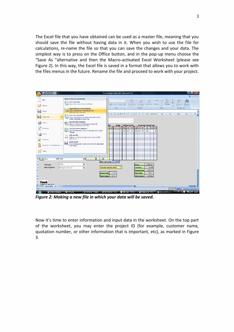
The Excel file that you have obtained can be used as a master file, meaning that you should save the file without having data in it. When you wish to use the file for calculations, re-name the file so that you can save the changes and your data. The simplest way is to press on the Office button, and in the pop-up menu choose the “Save As “alternative and then the Macro-activated Excel Worksheet (please see Figure 2). In this way, the Excel file is saved in a format that allows you to work with the files menus in the future. Rename the file and proceed to work with your project.

Figure 2: Making a new file in which your data will be saved. Now it’s time to enter information and input data in the worksheet. On the top part of the worksheet, you may enter the project ID (for example, customer name, quotation number, or other information that is important, etc), as marked in Figure 3.

4

Figure 3: Project information can be entered in the white zone on the top of the worksheet. The colours of the program have a certain meaning. In cells that are marked yellow, you can enter or change numbers. Cells that have other colours cannot be changed. The first column is called “Loop” (column B in the Excel file). This column allows the loop numbers to be changed. The default setting is “manifold nr : loop nr”, for example “1:3” means the third loop on manifold 1. You can change to other numbers or expressions in this column. If you wish to insert other symbols than numbers, you may need to place quote marks around the symbols (for example “1:A” rather than just 1:A). In the second column, the type of system used can be chosen from a scroll menu (column C in the Excel file). There is a variety of systems, each having different pipe spacing, pipe dimensions and panel thickness. Usually, the same type of panel is used in a project. The names of the panels follow a certain pattern. These are called Panels and are followed by four numbers. The first two numbers indicate the external diameter of the pipe and the latter two numbers represent the height of the panel (the measures are in millimetres). The last four characters represent the pipe spacing, also in millimetres. So, when the following panel is shown:

Panel 1625 s192 it means that a 16 mm pipe is used, with a spacing of 192 mm, and that the panel is 25 mm high.

5

In the same manner, Panel 1213 s192 is the thin panel, building 13 mm in height and has a 12 mm pipe with the spacing 192 mm. A third column (column D in the Excel file) has a scroll menu for the choice of material layers that are put onto the floor heating panel. In a project, various zones in the building can have different materials. Note that the surface materials have a large influence on the water temperatures. A value of the thermal resistance of the sub-floor must be entered in the fourth

column (E in the Excel file). This parameter is called “RT” and has the unit m²K/W. If the U-value of the floor construction is known, the thermal resistance is the inverse of the U-value. If the U-value is not known, there is in the program a spread sheet that helps to calculate the R-value if the size of the building and the material types and thickness are given (please see Figure 4 on how this is accessed).

Figure 4: The spreadsheet “RT” for calculation of floor construction thermal resistance can be accessed by clicking on RT at the bottom left side of the Excel interface. The R-values are in this case calculated according to standard EN ISO 13370 (2007)

Thermal performance of buildings – Heat transfer via the ground – Calculations methods.It is possible to calculate the thermal resistance for:

Intermediate floors (suspended floors between storeys)

Slab on ground

Cellars

Crawl spaces

6

The input required is the thickness of various material layers and occasionally the geometry of the foundation of the building (please see Figure 5). When the RT-value is established (see the dark blue field on the right hand side of the display), that value can be entered in the previous worksheet.

Figure 5: Snapshot of two tables used for calculating the thermal resistance of constructions underneath the panels. Going back to the worksheet “Manifold1”, the RT-value is entered in column E. In the next column F, the design indoor temperature is to be given. Column G is for the design temperature that is below or surrounds the construction underneath the floor heating system. This may be an indoor temperature if the construction is an intermediate floor that separates one apartment from the other. It may be the mean outdoor temperature of the heating season if the construction is a slab on ground. In other words, it is not evident that the temperature that is entered in this column is the design outdoor temperature. In the next column, I, the heating or cooling requirement at design conditions has to be given to the program. This value is usually calculated on basis of heat losses due to transmission – U-values and thermal bridges ((∑ ∑ ) ( )) - and ventilation( ( )) and divided by the heated floor area. In case of heating, the value is positive. In the case of cooling, the value is negative. The design temperature drop is entered in column J. Commonly the temperature drop is given values between 5 – 10 °C. In Flooré projects, 7 °C is often chosen at design conditions. Again, in case of heating, the value is positive and is negative for cooling.

Intermediate floor Thickness Choose material layer Resistance

(m) (m²×K/W)

0 -

0 -

0 -

0 -

0 -

0 -

0 - RT = - m²×K/W

0 -

Slab on ground Thickness Material layers in construction Resistance Joint between wall and slab

(m) excluding the ground (m²×K/W)

Input length (m): 0 0 -

Input width (m): 0 0 - y = 0 W/m×K

0 -

0 -

0 - Ground type

0 -

0 -

0 -

Sum: - RT = - m²×K/W

U-value: - W/m²×K

Material data

Material data

Material data

Material data

Material data

Material data

Material data

Material data

Material data

Material data

Material data

Material data

Material data

Material data

Material data

Material data

Choose thermal bridge type

Morene

7

Finally, pipe lengths are given in the last two columns, L and M. Ln in column L is part of the pipe that does not emit energy. A default value of 2 m is used, representing where the pipe leaves the floor and is connected to the manifold. This part does not participate in the heat balance of the building, but generates a pressure loss. In column M, the length of the pipe that actively emits or absorbs heat is to be inserted. With this done, the necessary input for a loop is completed. Let’s look at an example of what comes next. In Figure 6, the thin system with panel 1617 s192 is used in two loops. One loop is covered with tiles and the other with 15 mm parquet. The rest of the input data is the same for the two loops. When the values have been entered, there appears a number for each loop in column P. This is the optimum supply temperature for the loop, based on the input data. In this case, the wood floor will require 47 °C while the tile floor only needs 38 °C to fulfil the same requirement. When connected to the same manifold, we have to choose a common supply temperature for both loops. Therefore, you find on row 19 the text “Choose supply temp” and in red choose. If a supply temperature is not chosen, no results are displayed in the table.

Figure 7: A common supply temperature has to be chosen for the loops of the manifold. By giving the maximum supply temperature, all heating requirements will be fulfilled. Here, the value of 47 °C is given and all calculated values for the loops are shown. We find out the following:

In column T, the fulfilled requirements are displayed. For the wood floor, the required 60 W/m² are supplied. However, since the supply water temperature is higher than the optimal for the tiled floor, the current status will be able to fulfil 96 W/m². This loop will need a thermostat to reduce heat emission. Alternatively, the design temperature drop in column J can be increased.

Lengths Temps Heating /cooling Flows and pressure loss

Loop System Surface RT Ti Te Req DT Ln La Ltot To Ts Tr Req Tot Pow Dp Flow Kv dp Turns Vol

nr. Type Material m²K/W °C °C W/m² °C m m m °C °C °C W/m² W/m² kW kPa l/min m³/h mbar lit

1:1 3 20 0 60 7 2 70 72 38 - - - - - - - - - - -

1:2 3 20 0 60 7 2 70 72 47 - - - - - - - - - - -

1:3 - - - - - - - - - - - - - - - - - - - -

1:4 - - - - - - - - - - - - - - - - - - - -

1:5 - - - - - - - - - - - - - - - - - - - -

1:6 - - - - - - - - - - - - - - - - - - - -

1:7 - - - - - - - - - - - - - - - - - - - -

1:8 - - - - - - - - - - - - - - - - - - - -

1:9 - - - - - - - - - - - - - - - - - - - -

1:10 - - - - - - - - - - - - - - - - - - - -

Max opt temp: 47 °C

Fluid type Power 0,00 kW

Pipe roughness Choose supply temp: - °C choose Total flow 0 l/min

Pressure loss 0,0 kPa

Supply temp - °C Pipe length 144 m

Return temp 0 °C Fluid volume 0,0 liters

Panel 1617 s192

None

Panel 1617 s192

None

None

None

None

None

None

Tiles 8-12 mm

Parquet 15 mm; paper felt; PE-foil

None

None

None

None

None

None

None

None

Water

PEX pipes 0,007 mm

None

8

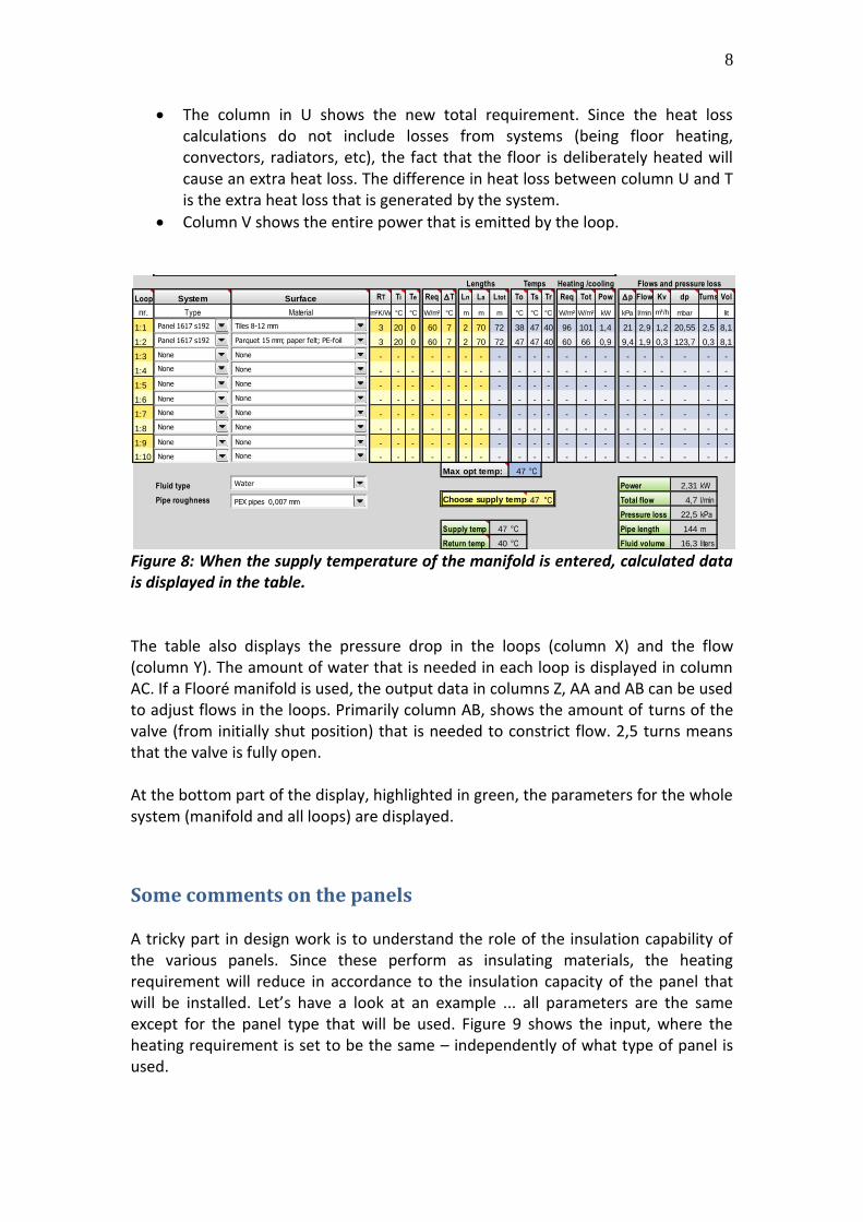
The column in U shows the new total requirement. Since the heat loss calculations do not include losses from systems (being floor heating, convectors, radiators, etc), the fact that the floor is deliberately heated will cause an extra heat loss. The difference in heat loss between column U and T is the extra heat loss that is generated by the system.

Column V shows the entire power that is emitted by the loop.

Figure 8: When the supply temperature of the manifold is entered, calculated data is displayed in the table. The table also displays the pressure drop in the loops (column X) and the flow (column Y). The amount of water that is needed in each loop is displayed in column AC. If a Flooré manifold is used, the output data in columns Z, AA and AB can be used to adjust flows in the loops. Primarily column AB, shows the amount of turns of the valve (from initially shut position) that is needed to constrict flow. 2,5 turns means that the valve is fully open. At the bottom part of the display, highlighted in green, the parameters for the whole system (manifold and all loops) are displayed.

Some comments on the panels A tricky part in design work is to understand the role of the insulation capability of the various panels. Since these perform as insulating materials, the heating requirement will reduce in accordance to the insulation capacity of the panel that will be installed. Let’s have a look at an example ... all parameters are the same except for the panel type that will be used. Figure 9 shows the input, where the heating requirement is set to be the same – independently of what type of panel is used.




1:1 3 20 0 60 7 2 70 72 38 47 40 96 101 1,4 21 2,9 1,2 20,55 2,5 8,1

1:2 3 20 0 60 7 2 70 72 47 47 40 60 66 0,9 9,4 1,9 0,3 123,7 0,3 8,1

1:3 - - - - - - - - - - - - - - - - - - - -

1:4 - - - - - - - - - - - - - - - - - - - -

1:5 - - - - - - - - - - - - - - - - - - - -

1:6 - - - - - - - - - - - - - - - - - - - -

1:7 - - - - - - - - - - - - - - - - - - - -

1:8 - - - - - - - - - - - - - - - - - - - -

1:9 - - - - - - - - - - - - - - - - - - - -

1:10 - - - - - - - - - - - - - - - - - - - -



Pipe roughness Choose supply temp:47 °C Total flow 4,7 l/min


Supply temp 47 °C Pipe length 144 m


Panel 1617 s192

None

Panel 1617 s192

None

None

None

None

None

None

Tiles 8-12 mm

Parquet 15 mm; paper felt; PE-foil

None

None

None

None

None

None

None

None

Water

PEX pipes 0,007 mm

None

9

Figure 9: The only difference in input is the panel thickness. The optimal temperatures increase with panel thickness! As seen in Figure 9, the optimal supply temperature increases with the thickness of the panel – which seems to be in contradiction to the function of increased thermal insulation. However, there is one aspect that has not been considered here – and that is the influence of the increased insulation on the heating requirement, which in this case is the same (60 W/m²). The thermal insulation of the various panels is shown in Table 1. Observe that the pipe size and spacing have influence on the insulation value – obviously increased pipe size decreases the insulation performance.

Table 1: Panel type and estimated thermal resistance of each panel.

Panel type Thermal resistance

[m²K/W]

Panel 1213 s192 0,192

Panel 1213 s120 0,102

Panel 1225 s192 0,672

Panel 1250 s192 1,440

Panel 1617 s192 0,242

Panel 1625 s192 0,609

Panel 1650 s192 1,410

Now, if the original construction has the thermal resistance RT = 3,00 m²K/W, this value will increase if extra insulation is placed on it. Also, the heating requirement will reduce, since the transmission loss through the floor will be reduced. The changes due to the insertion of panels are displayed in Table 2.




1:1 3 20 -15 60 7 2 70 72 37 - - - - - - - - - - -

1:2 3 20 -15 60 7 2 70 72 38 - - - - - - - - - - -

1:3 3 20 -15 60 7 2 70 72 39 - - - - - - - - - - -

1:4 - - - - - - - - - - - - - - - - - - - -

1:5 - - - - - - - - - - - - - - - - - - - -

1:6 - - - - - - - - - - - - - - - - - - - -

1:7 - - - - - - - - - - - - - - - - - - - -

1:8 - - - - - - - - - - - - - - - - - - - -

1:9 - - - - - - - - - - - - - - - - - - - -

1:10 - - - - - - - - - - - - - - - - - - - -



Pipe roughness Choose supply temp: - °C choose Total flow 0,0 l/min


Supply temp - °C Pipe length 216 m


Panel 1617 s192

Panel 1650 s192

Panel 1625 s192

None

None

None

None

None

None

Tiles 8-12 mm

Tiles 8-12 mm

Tiles 8-12 mm

None

None

None

None

None

None

None

Water

PEX pipes 0,007 mm

None

10

Table 2: Change in values due to the panels.

Panel type New RT

[m²K/W]

New qreq [W/m²]

Panel 1617 s192 3,242 59,1

Panel 1625 s192 3,609 58,0

Panel 1650 s192 4,410 56,3

The nominal heating requirement in the example is 60 W/m². Within this requirement, the heat loss through the floor construction is included. This loss can be estimated through the equation

( )

(1)

In our case, this corresponds to (keep in mind totally 60 W/m²)

( ( ))

⁄ (2)

Since the value of RT in Equation 1 will increase, the total heating requirement by means of Equation 2 will decrease, as shown in Table 2. Usually, for the thin panels 1213 and 1617, it is not practically justified to make the corrections since the thermal insulation of these panels are basically negligible. Insertion of the new values in the calculation procedure is illustrated in Figure 10. Here, the choice of the supply temperature is also inserted – since this value is common for all solutions (the supply temperature is important to fulfil heating requirement above the floor, whereas ground heat losses are compensated by increased water flow in the loop). The results become logical after correction of the heating requirement.

Figure 10: New values based on a corrected heated requirement.




1:1 3 20 -15 60 7 2 70 72 42 43 36 62 67 0,93 9,6 1,9 1,2 9,0 2,5 8,1

1:2 3 20 -15 58 7 2 70 72 43 43 36 58 61 0,85 8,7 1,7 0,8 16,9 0,9 8,1

1:3 3 20 -15 56 7 2 70 72 43 43 36 57 60 0,83 8,5 1,7 0,7 18,8 0,8 8,1

1:4 - - - - - - - - - - - - - - - - - - - -

1:5 - - - - - - - - - - - - - - - - - - - -

1:6 - - - - - - - - - - - - - - - - - - - -

1:7 - - - - - - - - - - - - - - - - - - - -

1:8 - - - - - - - - - - - - - - - - - - - -

1:9 - - - - - - - - - - - - - - - - - - - -

1:10 - - - - - - - - - - - - - - - - - - - -



Pipe roughness Choose supply temp: 43 °C Total flow 5,3 l/min


Supply temp 43 °C Pipe length 216 m


Panel 1617 s192

Panel 1650 s192

Panel 1625 s192

None

None

None

None

None

None

Laminate 8 mm; paper felt; PE-foil



None

None

None

None

None

None

None

Water

PEX pipes 0,007 mm

None

11

The results show that the thicker panels give a substantially reduced total heating requirement (called Tot, column U and also seen in Pow, column V). The difference in requirement is simply due to that the ground losses are less with the thicker panels. Please note that all values that are shown (and also the inserted supply temperature) do not show decimal values – and may appear irregular when rounded off to the nearest integer.

12

APPENDIX 1

Flooré design program model

Aim This report presents the model that is used in Floorés design program. The model considers upward heat dissipation, downward losses (including the loss due to that the floor is heated by the system) and system temperatures. The temperature drop along a loop is estimated with an exponential function.

A star-circuit model Underlying assumptions in the model are the following:

The model uses a steady-state approach;

The temperatures of the internal and external environments are uniform (constant) in time and in space;

The heating requirement is uniform in the zone. The following input is needed for the model to give results:

The heating requirement of the zone (transmission and ventilation loss) calculated on basis of heated floor area;

Design temperature drop along the loop;

Design internal and external environment temperatures;

The thermal resistance of the floor construction below the floor heating system.

The model is based on a thermal resistance star circuit, as displayed in Figur 1.1. Temperatures are represented by the symbol , thermal resistances by R and heat flows by . Index i stands for ”internal environment”, index e for ”external environment” (this may be the annual mean ground temperature or a calculated crawlspace temperature or temperature of a heated zone) and index s for “source”,

in this case the water temperature. Star circuit temperature n is a representative

temperature of the plane where the pipes are situated and has no direct relevance as a design parameter (it is more a model parameter).

13

Since the temperature of the water decreases whilst travelling in the pipe, it is important to account for which source temperature is considered. Therefore, this temperature will be a function of the distance from pipe inlet, here represented by x .

i

e

xs

eR

iR

hR

h

i

e

xn

Figure 1.1: The star-shaped thermal resistance network representing the flow paths

of heat in the floor construction.

For a ”slice” of the floor construction which is studied at a distance x from the loop’s inlet and having the thickness dx and the width s (the pipe spacing), the heat flow occurring upward (here denoted by the small heat flow ) through the floor surface is

in

i

i xR

dxs

= W (1.1)

In the same manner, the downward loss is

en

e

e xR

dxs

= W (1.2)

The total heat flow through the pipe, which compensates for the upward and

downward heat flows, passes through the thermal resistance hR . This thermal

14

resistance accounts for the construction (including the systems) ability to conduct heat sideways. However, it is defined on basis of the floor surface, area i.e. per square meter flooring. The law of energy conservation gives that

xxx eih = W (1.3)

So that

en

e

in

i

h xR

dxsx

R

dxsx

= W (1.4)

The heat transfer h from the bulk water temperature in the pipe, to the star

circuits temperature xn , passes through hR according to the following:

xxR

dxsx ns

h

h

= W (1.5)

By solving for xn , equation 5 will give that

dxs

Rxx hh

sn

=

Co (1.6)

Insertion of the expression for xn in equation 1.4 will render the following

equation,

=

ei

h

e

e

i

i

ei

s

h

RRR

RRRRxdxs

x11

1

11

W (1.7)

However, the heat that is transmitted through hR comes from water in the pipe that

is losing temperature over the distance dx . The change in temperature is denoted

by sd and is negative when the temperature drops along the loop.

The relationship between heat flow and temperature drop is

xdcMx spwh = W (1.8)

15

where M is the mass flow rate of water in the pipe and pwc is the specific heat

capacity of water. In combination with equation 1.3, the temperature drop is dependent on the internal and external temperatures (as seen in Figure 1.2), as well as the thermal resistances. Insertion of equation (1.8) into equation (1.7) gives after some tidying up that

=

h

ei

ei

pw

e

e

i

i

ei

ei

s

s

RRR

RRcM

dxs

RRRR

RRx

xd

(1.9)

Special attention is given to the term which here is named ekv , here defined as

=

e

e

i

i

ei

eiekv

RRRR

RR Co (1.10)

The general solution of the integral of equation 9 is given as

=h

ei

eipw R

RR

RRcM

xs

ekvinekvs ex

Co (1.11)

Figure 1.2: Temperature drop of the water during the distance dx. The drop is due to heat emission to the internal and external environment.

dx

s

i

e

0 L

Distance

Temp

i

e

ds

16

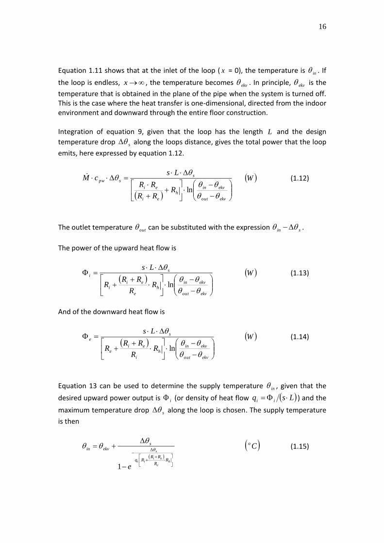
Equation 1.11 shows that at the inlet of the loop ( x = 0), the temperature is in . If

the loop is endless, x , the temperature becomes ekv . In principle, ekv is the

temperature that is obtained in the plane of the pipe when the system is turned off. This is the case where the heat transfer is one-dimensional, directed from the indoor environment and downward through the entire floor construction. Integration of equation 9, given that the loop has the length L and the design

temperature drop sD along the loops distance, gives the total power that the loop

emits, here expressed by equation 1.12.

D=D

ekvout

ekvin

h

ei

ei

s

spw

RRR

RR

LscM

ln

W (1.12)

The outlet temperature out can be substituted with the expression sin D .

The power of the upward heat flow is

D=

ekvout

ekvin

h

e

ei

i

s

i

RR

RRR

Ls

ln

W (1.13)

And of the downward heat flow is

D=

ekvout

ekvin

h

i

ei

e

s

e

RR

RRR

Ls

ln

W (1.14)

Equation 13 can be used to determine the supply temperature in , given that the

desired upward power output is i (or density of heat flow Lsq ii = ) and the

maximum temperature drop sD along the loop is chosen. The supply temperature

is then

D

D=

he

eiii

s

RR

RRRq

s

ekvin

e

1

Co (1.15)

17

The density of heat flow (heat flux), iq , is calculated from the heating requirement

at design conditions, Lsq designdesign = according to the following equation:

eigdesigni Uqq = 2mW (1.16)

where the U-value of the floor/ground construction in essence is

ei

gRR

U

1

KmW 2 (1.17)

This U-value can be estimated by use of EN ISO 13370:2007 “Thermal performance of buildings - Heat transfer via the ground - Calculation methods”

Note that eidesign , in other words, that the sum of heat emitted upward

and downward are larger than the heating requirement of zone. The reason is that a heat loss calculation at design conditions, that yields design , does not consider the

fact that the floor construction is actively heated. By heating the construction, an extra heat loss is generated. This heat loss is quantified by the following equation, such that

e

eekv

ekvout

ekvin

h

i

ei

e

s

extraR

RR

RRR

q

D=

ln

2mW (1.18)

or

eig

ekvout

ekvin

h

i

ei

e

s

extra U

RR

RRR

q

D=

ln

(1.19)

Determining the thermal resistances of the star-circuit

The resistances in the star-network model can be obtained by two means:

To perform heat power and temperature measurements;

And/or to perform simulations of two dimensional heat flow in constructions with integrated heat sources.

As measurements require immense resources, simulations are faster and easier to analyse. However, simulations may not be reliable since a number of assumptions

18

have to be performed. The most effective method is to combine measurements and simulations. The working steps used here are the following:

Perform measurements on a limited amount of pre-defined cases. Measurements involve monitoring supplied power and temperatures under controlled environmental conditions;

Analyse measurement data to validate simulation models;

Perform simulations for a large number of cases based on the experience and validated models from the measurements.

This procedure is common. Experience from a field trial and finite difference models for a constant power cable for the Flooréco system are available from the Marma project (Akander et al 1994). By using verified models, simulations can be used for multiple types of floor constructions and flooring materials. The results are used to adapt the parameters of

the star-model for effective use. The important parameters to calculate are hR and

iR . The resistance under the floor heating system, eR , can be estimated by using U-

value calculations as specified by EN ISO 13370:1998 (heat loss to the ground) or for intermediate floors with traditional one-dimensional U-value calculations. Finite difference modelling When modelling in finite differences, work is facilitated if a representative part/portion of the actual system is considered, see for example (Blomberg 1996). Floor heating systems are repetitive in layout, so it is more resourceful to select a small section instead of modelling the entire volume in which the floor heating system is installed. The only exception for this is in areas that may contain thermal bridges, such as joints between suspended floors and external walls where the degree of insulation locally in the wall is small or non-existent. In floor heating applications, two dimensional heat transfer programs are sufficient for effective and accurate modelling. The choice of which part of the system that is considered to be representative is dependent on the symmetry of the isotherms in the construction. Commonly, this is found within the distance of a half spacing distance way from the pipes, as shown in figure 1.3.

19

s

Figure 1.3: Cross section of a floor construction with a surface-mounted floor heating system where pipe spacing has the value s . The dark frame depicts an area with isotherms that is symmetric with neighbouring pipes. The dashed frame shows the symmetric area for the considered cable. The area within the dashed frame is entered as a model in the finite difference program. Required data are material geometry (material layer thickness), material thermal conductivity and suitable boundary conditions. Two calculations have to be performed per construction and system type, in which the boundary conditions are varied. For the upper surface, the interior surface thermal resistance has to be given a value. In practical calculations, a value of 0,09 –

0,10 m2K/W can be used. More exact values are given by an equation in EN 1264.

The boundary conditions are illustrated in Figure 4 with values specified in Table 1.1 for the two calculations. Adiabatic surface means that there is no heat exchange with the surroundings (no heat passes the surface).

20

Table 1.1: Combinations of boundary conditions to calculate thermal resistances of the star-network. The heat flow densities are defined as positive in the flow direction as viewed in Figure 1.

Case Upper surface

Lower surface

Pipe surface

Calculated heat flow from numeric model

1 1 C 0 C Adiabatic 1i W

2 0 C 0 C 1 C 2i and 2e W

s/2

Adiabat

Adiabat

Upper surface boundary

Lower surface boundary

Pipe surface boundary

Figure 1.4: The boundary conditions of a typical model of a floor heated construction. When the calculations have been performed, the sets of equations as listed below will give the thermal resistances, provided that 1i , 2i and 2e have been

calculated according to the boundary conditions expressed in Table 1.1.

221

22

eii

e

i

sR

= WKm 2 (1.20)

=

2

221

22

22

12

eii

ei

ei

h sR WKm 2 (1.21)

221

22

eii

i

e

sR

= WKm 2 (1.22)

21

References Akander J., Lacour C., Mao G. and Johannesson G. (1994). Ett elbaserat golvvärmesystem – Mätningar och beräkningsmodeller. Dept. of Building Technology, KTH, Stockholm, Sweden. (In Swedish). Blomberg T. (1996). Heat condution in two and three dimensions – Computer modelling of building physics applications. Report TVBH-1008. Dept. of Building Physics, LTH, Lund, Sweden. EN ISO 13370 (2007). Thermal performance of buildings – Heat transfer via the ground – Calculations methods. European Committee of Standardisation (CEN), Brussels, Belgium.

design program in excel for flooré panel products manual...

Documents