ii

AUTHOR'S DECLARATION

I hereby declare that I am the sole author of this thesis. This is a true copy of the thesis,

including any required final revisions, as accepted by my examiners.

I understand that my thesis may be made electronically available to the public.

iii

Abstract

In this thesis, we describe the design of tubular network systems that must occupy, as best

as possible, regions that demonstrate some kind of longitudinal symmetry. In order to

simplify the problem, the region of the container is discretized into a sequence of prism

blocks 𝐵1, 𝐵2, …𝐵𝑁. The problem is decomposed into two parts: 1. Pack tubes in these

blocks, 2. Connect these packed tubes at the ends of each block.

In the first part, since each block is prismatic, the problem of packing tubes is equivalent to

the packing of circles in the cross-sectional area of each block. In this case, we assume that

the cross-sectional area of each block is a polygon. We investigate a series of algorithms to

pack circles, including a rather naive approach as well as the GGL [2] circle packing

algorithm. Then we modify the GGL algorithm to pack circles in regions that are more

complicated. Based on the GGL, we will also invent new algorithm that provides more

satisfactory packing results.

In the second part, we connect the packed tubes from Part one to form a complete network

system. First we consider the simplest case -- constructing a tubular system in a container

with no variations, i.e., a single block. We solve this problem in terms of the travelling

salesman problem (TSP) which is a classical problem in discrete optimization. For containers

with varying cross-sections, we connect tubes at end of each block independently instead of

constructing a complete system. This problem can be reduced to a perfect matching (PM)

problem at each end. We apply similar integer programming algorithms to both perfect

matching problem and TSP. However, the design of complete tubular network system in a

container exhibiting longitudinal symmetry remains an open problem for future work.

iv

Acknowledgements

First and foremost, I would like to express my sincere gratitude to my co-supervisors, Dr.

Edward Vrscay and Dr. Franklin Mendivil, as well as Dr. Sean Peterson, for their support,

guidance and care. I would also thank our group members Wenzhe Jiang and Brian

Kettlewell for their excellent ideas and inspiration. In addition, I especially thank my friend

Yinuo Liu from the Department of Computational Mathematics for his support on the C++

implementation of matching algorithm. I also wish to thank Dr. William Cook who is a

professor at the Department of Combinatorics and Optimization for his extraordinary

courses on discrete optimization (CO 650 Combinatorial Optimization and CO 759

Computational Discrete Optimization).

I would also like to acknowledge the financial support from the Faculty of Mathematics,

University of Waterloo, the Department of Applied Mathematics, University of Waterloo

and an NSERC Collaborative Research and Development Grant.

v

Table of Contents

AUTHOR'S DECLARATION ...........................................................................................................ii

Abstract ..................................................................................................................................... iii

Acknowledgements ................................................................................................................... iv

Table of Contents ....................................................................................................................... v

List of Figures ............................................................................................................................ ix

List of Tables ............................................................................................................................. xii

List of Abbreviations ............................................................................................................... xiii

Chapter 1 Introduction .............................................................................................................. 1

Chapter 2 Circle-Packing ........................................................................................................... 6

2.1 A Very Naïve Approach to the Packing Problem ............................................................. 6

2.1.1 Bounding Box of a Region ......................................................................................... 7

2.1.2 Fill the Bounding Box with Circles ............................................................................ 9

2.1.3 Deleting Circles ....................................................................................................... 10

2.1.4 Summary of the Naïve Approach ........................................................................... 11

2.2 The Dawn: GGL-based Circle-Packing Scheme [2]......................................................... 12

2.2.1 Basic Concepts and Notations ................................................................................ 13

2.2.2 Rules and Formulas for Packing Circles .................................................................. 14

2.2.3 Possible Positions of Placing a Circle ...................................................................... 20

2.2.4 Position Strings ....................................................................................................... 23

2.2.5 Some Numerical Experiments of Original GGL Algorithm ...................................... 25

2.3 Modified GGL-Packing ................................................................................................... 27

2.3.1 GGL in Trapezoidal Regions ..................................................................................... 27

2.3.2 GGL in L-shaped Regions ........................................................................................ 31

2.3.3 Future of the GGL Circle-Packing Scheme .............................................................. 34

2.4 New Packing Scheme Based on GGL ............................................................................. 34

2.4.1 Defining an Arbitrary Polygon................................................................................. 35

vi

2.4.2 Polygon’s Area ........................................................................................................ 36

2.4.3 Anti-GGL Scheme [6] .............................................................................................. 37

2.4.4 Position Number in Anti-GGL Scheme .................................................................... 39

2.4.5 Constraints in Polygon ............................................................................................ 40

2.4.6 Some Numerical Experiments of Anti-GGL Scheme ............................................... 44

2.4.7 Summary of Anti-GGL ............................................................................................. 45

2.5 Packing in a Shrunken Polygon ...................................................................................... 46

2.5.1 Problem Description ............................................................................................... 46

2.5.2 Compute the Vertices of P’ ..................................................................................... 47

2.6 Summary of the Chapter ............................................................................................... 50

Chapter 3 Preparations for Connection .................................................................................. 51

3.1 Fundamental Elements .................................................................................................. 51

3.2 End-caps and Interference ............................................................................................ 54

3.2.1 Interference ............................................................................................................ 55

3.2.2 Interference Ratio ................................................................................................... 56

3.2.3 Interference Tolerance ............................................................................................ 58

3.2.4 Approaches to Interference .................................................................................... 58

3.2.5 The New Element: Modified L-block ...................................................................... 60

3.3 Graph Representation for Possible Connection ............................................................ 62

3.4 Moving towards the Connection Problem .................................................................... 65

Chapter 4 One-Path Network and Travelling Salesman Problem (TSP) .................................. 67

4.1 One-Path Network System ............................................................................................ 67

4.1.1 Hamiltonian Cycle ................................................................................................... 69

4.1.2 Corresponding Hamiltonian Path to a One-path Network System......................... 70

4.1.3 Weighted Hamiltonian Path.................................................................................... 72

4.1.4 TSPP≡ 𝒑TSP ............................................................................................................ 73

4.1.5 From Practical to Abstract ...................................................................................... 74

vii

4.2 Subtour Elimination with Branch and Cut Algorithm for TSP [14][15] .......................... 75

4.2.1 Characteristic Vector and Integer Programming .................................................... 76

4.2.2 Linear Programming Relaxation .............................................................................. 76

4.2.3 Difference between Subtour and TSP Tour ............................................................ 78

4.2.4 Cutting Plane Method [14] ..................................................................................... 78

4.2.5 Branch and Cut [15] ................................................................................................ 80

4.2.6 Some Thoughts on the Algorithm for TSP .............................................................. 81


Chapter 5 Connections in Varying Cross-sections ................................................................... 84

5.1 Operations between Tubes [24] .................................................................................... 85

5.1.1 Connection between Operations ........................................................................... 87

5.2 Cutting Plane for Matching [26] .................................................................................... 88

5.2.1 A General View of the Cutting Plane Method for Perfect Matching (PM) ............. 89

5.2.2 Step 1-Step 4 and Step 6-7: General Process of Cutting Plane Method ................. 92

5.2.3 Step 5: Odd Cuts in G* ............................................................................................ 92

5.2.4 Termination of Algorithm 8 .................................................................................... 94

5.2.5 Running Time of Algorithm 8 .................................................................................. 95

5.3 Bifurcation End-cap and b-matching ............................................................................. 96

5.3.1 Solving b-matching ................................................................................................. 98


Chapter 6 Conclusion and Future Works .............................................................................. 101

6.1 Conclusions .................................................................................................................. 101

6.1.1 Part 1: Circle Packing ............................................................................................ 101

6.1.2 Part 2 Connection between Tubes........................................................................ 102

6.1.3 Emphasizing the Difference between This Thesis and [24] .................................. 104

6.2 Future Works ............................................................................................................... 104

6.2.1 Non-simple Connected Cross-section................................................................... 104

viii

6.2.2 Weights on Connection Graph.............................................................................. 105

6.2.3 Connection Graph of System ................................................................................ 105

6.2.4 CAD Work for Tubular Network System ................................................................ 106

Appendix A Derivation the parameterization of modified L-block ....................................... 108

Appendix B Improvement of Algorithm 7 ............................................................................. 110

Appendix C Algorithm 9 Cutting Plane and Branch and Cut for TSP (Pseudocode) ............. 112

Appendix D Blossom Inequality of Cut Form ........................................................................ 113

Bibliography .......................................................................................................................... 114

ix

List of Figures

Figure 1 Redneck barbeque pool heater [1] ..................................................................... 1

Figure 2 Discretized region V ............................................................................................ 2

Figure 3 Parallel tubes in each Bi ...................................................................................... 2

Figure 4 Bounding box of a closed region ......................................................................... 7

Figure 5 Put circle in the center ........................................................................................ 9

Figure 6 Put a circle next to first one ................................................................................ 9

Figure 7 Fill the rectangle with circles ............................................................................... 9

Figure 8 Ray intersects edges odd times, z is inside ....................................................... 11

Figure 9 Ray intersects edges even times, z is outside ................................................... 11

Figure 10 Delete infeasible circles, dash lane circles are deleted ................................... 12

Figure 11 Side of rectangle ............................................................................................. 13

Figure 12 Position No.1, Bottom left .............................................................................. 15

Figure 13 Position No.2, lower right corner .................................................................... 15

Figure 14 Tangent to side 1 and circle i ........................................................................... 16



Figure 17 Packing a circle between a and b .................................................................... 18

Figure 18 Triangle formulized by centers ........................................................................ 18

Figure 19 GGL Experiment 1 ........................................................................................... 25




Figure 23 Analysis Report of Experiment 4 ..................................................................... 27

Figure 24 Trapezoidal Region .......................................................................................... 28

Figure 25 Distance from a circle ...................................................................................... 29

Figure 26 Choosing a root with respect to the slope ...................................................... 30

x

Figure 27 L-shape region ................................................................................................. 31

Figure 28 Circle on the corner of side 3 and side 4......................................................... 33

Figure 29 Example of a polygon with displacement vectors .......................................... 35

Figure 30 Placement of first and second circle ............................................................... 38

Figure 31 All cases of two line segments ........................................................................ 42

Figure 32 A case around non-convex corner .................................................................. 43

Figure 33 Anti-GGL Experiment 1 ................................................................................... 45

Figure 34 Anti-GGL Experiment 2 ................................................................................... 45

Figure 35 An example of shrink polygon P to P' by d ...................................................... 47

Figure 36 Intersection of translated edge vector ............................................................ 48

Figure 37 Shrink Experiment 2 by 0.1 ............................................................................. 49

Figure 38 I-block .............................................................................................................. 52

Figure 39 L-block ............................................................................................................. 52

Figure 40 T-block ............................................................................................................. 53

Figure 41 Endcaps ........................................................................................................... 54

Figure 42 Interference of end-cap .................................................................................. 55

Figure 43 General formulization of interference ............................................................ 56

Figure 44 Narrowed end-cap .......................................................................................... 59

Figure 45 Bend with two radius ...................................................................................... 59

Figure 46 Modified L-block ............................................................................................. 60

Figure 47 End-cap of Modified L-block ........................................................................... 61

Figure 48 End-cap of two tubes with different radii ....................................................... 62

Figure 49 An example of connection graph .................................................................... 64

Figure 50 Small example of one-path system ................................................................. 68

Figure 51 Hamiltonian cycle in a connection graph ........................................................ 70

Figure 52 Relation between Hamiltonian path and a one-path network system ........... 71

Figure 53 Subtour of an integer solution ........................................................................ 77

xi

Figure 54 Difference of TSP and subtour ........................................................................ 77

Figure 55 A fractional solution with no subtour ............................................................. 79

Figure 56 Brach and cut .................................................................................................. 81

Figure 57 simple example on changing cross-sections ................................................... 84

Figure 58 The example in all 4 sections .......................................................................... 84

Figure 59 Single merge and its decomposition ............................................................... 85

Figure 60 Consecutive merge .......................................................................................... 85

Figure 61 Shift operation ................................................................................................ 86

Figure 62 Merge-shift-merge (MSM) .............................................................................. 86

Figure 63 An example of application of operations ........................................................ 87

Figure 64 Example of fractional solution in odd set ....................................................... 90

Figure 65 Running time results ....................................................................................... 96

Figure 66 Bifurcation end-cap ......................................................................................... 96

Figure 67 “T-block” in bifurcation end-cap ..................................................................... 97

Figure 68 Data reduction for b-matching ........................................................................ 98

Figure 69 Non-simple connected region ....................................................................... 105

Figure 70 Incomplete network system for 9-4-9 ........................................................... 106

Figure 71 3D model for 9-4-9 ........................................................................................ 106

xii

List of Tables

Table 1 Position number of circle i .................................................................................. 23

Table 2 Position number in anti-GGL .............................................................................. 39

xiii

List of Abbreviations

GGL George, George and Lamar [2]

TSP Travelling Salesman Problem

TSPP TSP path

IP Integer Programming

RLP Relaxed Linear Programming

MST Minimum Spanning Tree

GH Gomory-Hu Tree

PM Perfect Matching

MSM Merge-shift-merge

1

Chapter 1

Introduction

In this thesis, we will design a tubular network system in a longitudinal symmetry container.

This means that the surface container is constructed by lofting a branch of cross-sections along

a straight line (See Figure 3 , a discretized version of a container) . A practical example of this

network design is the following:

Figure 1 Redneck barbeque pool heater [1]

The tubular system in Figure 1 is embedded in a region enclosed by barbeque for the purpose

of heating water in a pool. There are one inlet and one outlet of the system. Water flows into

the system via the inlet; the stove heats the water stored in the system, and hot water will

come out from the outlet. From the figure, it can be seen that the barbeque was the shape of a

prism, which means that the cross-sections of the container are identical. In this network, only

one size of tube is used. The purpose of this thesis is to design a more generalized version of

the barbeque pool heater. For example, we want to design a network system with tubes of

multiple sizes. We also wish to consider the containers with varying cross-sections in the

longitudinal direction. In order to simplify such complicated region, we discretize the shape of

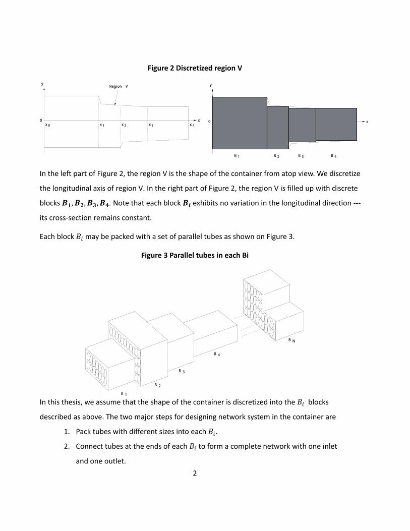
the container into finite blocks 𝐵1, 𝐵2 …𝐵𝑁 as shown in Figure 2 and Figure 3.

2

Figure 2 Discretized region V

In the left part of Figure 2, the region V is the shape of the container from atop view. We discretize

the longitudinal axis of region V. In the right part of Figure 2, the region V is filled up with discrete

blocks 𝑩𝟏, 𝑩𝟐, 𝑩𝟑, 𝑩𝟒. Note that each block 𝑩𝒊 exhibits no variation in the longitudinal direction ---

its cross-section remains constant.

Each block 𝐵𝑖 may be packed with a set of parallel tubes as shown on Figure 3.

Figure 3 Parallel tubes in each Bi

In this thesis, we assume that the shape of the container is discretized into the 𝐵𝑖 blocks

described as above. The two major steps for designing network system in the container are

1. Pack tubes with different sizes into each 𝐵𝑖.

2. Connect tubes at the ends of each 𝐵𝑖 to form a complete network with one inlet

and one outlet.

3

Chapter 2 discusses the mathematical aspects of step 1. Since each 𝐵𝑖 has constant cross-

section and each tube has circular cross-section, packing tubes into 𝐵𝑖 is equivalent to packing

circles into a closed planar region 𝐷𝑖 where 𝐷𝑖 is the cross-section of 𝐵𝑖. This problem is a

classical optimization problem called “circle packing”. (In Figure 3, the 𝐷𝑖 are rectangular, but in

this thesis, the 𝐷𝑖 are assumed to be arbitrary polygon). It is wellknown that packing unequal

circles into an arbitrary region is a NP-hard problem, which means there is no polynomial time

algorithm that can find an optimal packing in general. However, this does not mean that circle

packing is unsolvable. Some approaches such as greedy algorithm [13] and heuristic search [12]

can provide feasible packing in some particular regions such as circular regions. In Chapter 2, we

will investigate an algorithm developed by George, George and Lamer in 1995, to be referred as

GGL algorithm [2]. The GGL algorithm is a heuristic algorithm that packs unequal circles into a

rectangular region. We will generalize the GGL algorithm to more complicated region such as

trapezoid and L-shaped region. We will also develop a new algorithm that uses exactly the

opposite idea of GGL. This new algorithm will provide a packing that is more suitable for our

purpose as compared to GGL. Finally, we will develop another algorithm to keep packed circles a

prescribed distance away from the boundary of region.

After obtaining a packing, we need to connect these packed tubes. However, the information

of packed circles is not adequate for determining connections between tubes. For instance,

with only the information of packing, we cannot determine whether we allow two tubes to be

connected to one tube. Chapter 3 plays a role of translating the information of packing to a

mathematical instance for connection. In this chapter, we will define fundamental elements

for connection, and in the rest part of the thesis, all connections and operations are based on

these fundamental elements. Then we define a new criterion for connection. Based on this

new criterion, we will construct a graph instance that stores all the possibilities of connections,

and we call it the connection graph. In step 2 above, when we make decisions of connections,

we actually choose the edges from the graph. Therefore, Chapter 3 is a transition from step 1

to step 2.

4

The actual step 2 is discussed in Chapter 4 and Chapter 5. These two chapters have many

similarities: both of them correspond to a type of connection between tubes to a mathematical

instance in graph theory, and both of them apply similar combinatorial optimization algorithm

called the cutting plane algorithm to solve their respective problems.

In Chapter 4, we will focus on a network system in region with non-varying cross-sections, for

example, the barbeque pool heater. The system discussed in this chapter is one long tube that

connects every tube packed in the cross-section. We provide a correspondence between this type

of connection to the travelling salesman problem (TSP) in the connection graph. TSP is a classical

NP-hard problem. Numerous researches have been done on TSP in past fifty years. The best

deterministic algorithm is dynamical programming which is still 𝑂(𝑛22𝑛) [20]. Some non-

deterministic algorithm such as genetic algorithm [16] or heuristic algorithm [17] can also solve

TSP in small problem cases. In this chapter, we will solve TSP via a non-deterministic algorithm

based on integer programming [14].

Chapter 5 discusses tube connections in regions with varying cross-sections. Unlike Chapter 4,

the one long tube network is infeasible in this case. In fact, instead of designing the whole

tubular network, we find connections in each cross-section independently in this chapter. It is

reduced to another classical discrete optimization problem called perfect matching problem in

the connection graph of each cross-section. Fortunately, the perfect matching problem has a

𝑂(|𝑉|3) polynomial algorithm called the “blossom algorithm”, developed by Edmonds [31]. In

this chapter, we will solve matching problem via the similar integer programming method in

Chapter 4, and this algorithm is a deterministic for perfect matching.

Although we can find connections in each cross-section, assembling them may not yield a

feasible network system. Therefore, as Chapter 5 is the last chapter of this thesis, designing a

feasible network system in region with varying cross-sections still remains an open problem in

future.

The Matlab implementation of the GGL algorithm [2] and the anti-GGL algorithm [6] in Chapter

2 is the author’s own work. Dr. Sean Peterson gave advice for the idea of Chapter 3. The one-

5

path network system and C implementation of subtour elimination for TSP [14] are the author’s

own contributions. The first part of Chapter 5 (Section 5.1) comes from Wenzhe Jiang’s thesis.

[24] The C++ program of cutting plane for matching was written with the help of Yinuo Liu, a

Master’s student from the Department of Computational Mathematics at the University of

Waterloo.

There is one major difference between this thesis and MMath thesis of Wenzhe Jiang [24]

(which also solves the connection problem) which needs to be mentioned. In [24], the author

generates all possible networks for a given region to be occupied. From these networks, a

"best" network can be extracted. In this thesis, however, we reduce the design problem to a

problem involving graphs and then apply combinatorial optimization algorithms to find an

optimal solution. As such, the method described in this thesis produces only one "best"

tubular network system.

6

Chapter 2

Circle-Packing

The top priority in the design problem is to obtain a feasible tubular network with maximum

storage volume. Thus, the connection design between tubes is less important compared to the

cross-sectional area covered by straight tubes. In this problem, we assume that all the tubes

have circular cross-sections, and the cross-section area covered by tubes is now reduced to

pack circles in 𝑅2 into an arbitrary closed region D with maximizing the area covered by the

packed circles. However, this problem is generally NP-hard even in a rectangular or circular

region; that means there is no deterministic polynomial-time algorithm to solve this problem.

Some algorithms such as heuristic algorithm and greedy algorithm are described in [3]，[13]

and [12], but their algorithms either pack circles into a specific region i.e. circle region, or

require an intolerably large running time which will not help in this case. We need to pick an

algorithm and modify it to satisfy our requirement.

One more constraint that needs to be considered is the cost of tubes. Although the volume of

network is our top priority, we cannot ignore the cost of designing. Indeed, if volume is

everything, we can just pack the whole cross-section with very small circles; however, the

design cost of this packing is very large. In order to simplify the problem, we only allow three

fixed size circle, say the radii of circles are 𝑅1, 𝑅2, 𝑅3, to be packed in the region D.

Now the problem becomes of packing circles with three radii 𝑅1, 𝑅2, 𝑅3 into an arbitrary closed

region D with packing area to be maximized. It is still a very hard problem. We need to start

from something easy and solvable and then looking forward to the hard problem. A good start

is to try a very naive approach to packing circles of one size into a region D.

2.1 A Very Naïve Approach to the Packing Problem

Announcement: This section is the first attempt of packing circles. It is rough and simple, but it

is related to the actual circle packing we use in section 2.4.

7

Lao-tzu has a quote, “A journey of a thousand miles begins with a single step” [34]. Therefore,

every hard problem has a first approach. For our circle-packing problem, we can at least have a

try to put circles of one radius into some bounded region that cover our packing region D

completely, and remove the circles that be outside desired region. In order to implement the

approach, we need following four steps:

1. Generate a minimum-bounding box that covers the region.

2. Put first circle into the center of minimum-bounding box.

3. Try to fill the bounding box with circles.

4. Delete the circles with center outside the region D or touching the boundary of D.

It seems to be as easy as 1-2-3 that even a child can come up. However, its implementation is

not as easy as the idea. Several trade-offs and simplifications are necessary.

In the rest of the section, we assume that the boundary of D, 𝜕D, is parameterized as

(𝑥(𝑡), 𝑦(𝑡)), with 𝑡 ∈ [0, 𝐿]. D is the region inside 𝜕D.

2.1.1 Bounding Box of a Region

A bounding box of D is the rectangle that encloses D. As shown on Figure 4.

Figure 4 Bounding box of a closed region

In fact, as a mathematical problem, the 2-D bounding rectangle is not a hard problem. As we

parameterize 𝜕D= {(𝑥(𝑡), 𝑦(𝑡)), 𝑡 ∈ [0, 𝐿]}, the simplest case of the bounding box of D is the

rectangle region defined by {[min(𝑥(𝑡)) ,max(𝑥(𝑡))] × [min(𝑦(𝑡)) ,max(𝑦(𝑡))], 𝑡 ∈ [0, 𝐿]}. We

just need to compute the maximum and minimum value of x and y coordinate with t in the

8

interval [0, L]. The computation of maximum and minimum value of single variable function

can be found in any fundamental calculus textbook. We can compute the derivative of the

function and let it to be zero. Then compare the value of the function on zero derivative points

and endpoints.

Although maximum and minimum can be found by hand with simple calculus, it is barely

infeasible for computer to compute in analytical way. In numerical way, we have to use the

Algorithm 1 Golden Section Search Algorithm [9]

Let 𝝋 =√𝟓−𝟏

𝟐, set a tolerance, find min of f in [0,L]

1. Compute f(a) and f(b).

2. Let c=b+ 𝜑(a-b), d=a+ 𝜑(b-a), compute f(c) and f(d).

3. If f(c)<f(d), then set (b,f(b)):=(d,f(d)), (d,f(d)):=(c,f(c)), goto step 2 without computing

d.

4. If f(c)>=f(d), then set (a,f(a)):=(c,f(c)), (c,f(c)):=(d,f(d)), goto step 2 without computing

c.

5. Keep iterating until |c-d|<tolerance, then c or d is our minimum. ∎

The above algorithm is for computing the minimum. If we want to compute the maximum, we

just keep step 1,2,5 and modify step3 and step 4 as following:

3. If f(c)>f(d), then set (b,f(b)):=(d,f(d)), (d,f(d)):=(c,f(c)), goto step 2 without computing

d.

4. If f(c)<=f(d), then set (a,f(a)):=(c,f(c)), (c,f(c)):=(d,f(d)), goto step 2 without computing

c.

It should be noted that the algorithm might not converge if f does not have a maximum or

minimum. But it could not happen in our case since 𝜕D is a closed curve and 𝑥(𝑡), 𝑦(𝑡) are

always bounded.

9

In addition, the 3D bounding box problem is much more complicated than 2D case. Joseph

O'Rourke has a cubic time algorithm for 3D bounding box in 1985 [4], but it is beyond the

scope of this thesis

2.1.2 Fill the Bounding Box with Circles

This is the only step that we will use in the future discussion of circle packing. (In the Anti-GGL

packing, it is used to generate the first and second circle).

We will put our first circle into the geometry center of the bounding rectangle as shown in

Figure 5. Then we put a circle right tangent to it, as in Figure 6

Figure 5 Put circle in the center

Figure 6 Put a circle next to first one

Then we continue to put circles around these two circles’ four directions. It is easy to check if a

circle is inside a rectangle, we will discuss this in next section. We can stop packing when no

more circles can be placed in the rectangle, as shown in Figure 7.

Figure 7 Fill the rectangle with circles

Now we have a circle packing in the bounding box of the region instead of a circle packing in

the region. We then need to delete these circles that are not right packed in the region.

10

2.1.3 Deleting Circles

There are two situations in which we shall delete a circle:

1. Its center lies outside the region but inside the bounding box

2. Its center lies inside the region but it intersects with the boundary of the region

Case1: In the first case we need to determine if a point is inside a closed curve. Suppose we

have a point (𝑥0, 𝑦0) and we want to determine if it is in the closed curve 𝜕𝐷 =

{(𝑥(𝑡), 𝑦(𝑡)), 𝑡 ∈ [0, 𝐿]}. We can set the point in the complex plane, let 𝑧0 = 𝑥0 + 𝑦0𝑖,

consider the contour integral of the function 𝑓(𝑧) =1

𝑧−𝑧0 around contour 𝜕𝐷 with counter-

clockwise orientation,

∮ 𝒇(𝒛)𝝏𝑫

𝒅𝒛 = ∮𝟏

𝒛 − 𝒛𝟎𝝏𝑫

𝒅𝒛

Note that 𝑓(𝑧) is analytic in the whole complex plane except at 𝑧0. If 𝑧0 is inside 𝜕𝐷, then 𝜕𝐷

encloses a pole of 𝑓(𝑧) so that by Cauchy-Goursat theorem, the above integral is non-zero.

Otherwise, if 𝑧0 lies inside 𝜕𝐷, 𝑓(𝑧) is analytic inside 𝜕𝐷; and the above integral is zero.

Almost every elementary complex analysis book will teach how to evaluate the above integral by

hand. Problems arise, however, when we must must program to compute it. In fact, the numerical

algorithm for computing contour integral is not as efficient as single variable integration; most of

these algorithms employ linear interpolation to approximate 𝜕𝐷 by a polygon and then compute

the contour integral along the edges of the polygon. However, if we want to determine whether a

point lies inside a polygon, there is an algorithm that is more efficient than computing contour

integral:

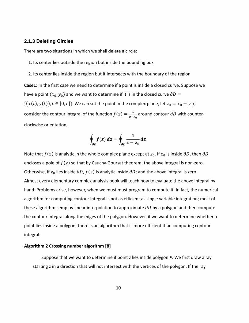
Algorithm 2 Crossing number algorithm [8]

Suppose that we want to determine if point z lies inside polygon P. We first draw a ray

starting z in a direction that will not intersect with the vertices of the polygon. If the ray

11

intersects the edges of the polygon an odd number of times, z lies inside P, as Figure 8.

Otherwise z is outside P as Figure 9.

Figure 8 Ray intersects edges odd times, z is inside

Figure 9 Ray intersects edges even times, z is outside

This algorithm needs to compute intersection of line segments (See Algorithm 5 Line Segment

Intersection). ∎

Case2: Recall that the second case assumes that the center of circle lies inside the region D.

However, the circle intersects 𝜕𝐷. To find these circles that intersects boundary, we need to

use the definition of circle. Since a circle is defined as a set of point that have equal distance to

a fixed point, we can compute the minimum distance of a circle’s center to edges of the

polygon; if the distance is strictly less than the radius of the circle, then it intersects 𝜕𝐷;

otherwise it does not intersect with 𝜕𝐷.

In 2D, computing the minimum distance between a point and a curve is not too hard. The

distance between point 𝑧0 = (𝑥0, 𝑦0) and curve 𝜕𝐷 = {(𝑥(𝑡), 𝑦(𝑡)), 𝑡 ∈ [0, 𝐿]} is defined as

min {𝑑(𝑡) = √(𝑥0 − 𝑥(𝑡))2+ (𝑦0 − 𝑦(𝑡))

2, 𝑡 ∈ [0, 𝐿]}

The distance function 𝑑(𝑡) is indeed a single variable function of t; to compute its minimum,

we can still use Algorithm 1 Golden Section Search Algorithm .

2.1.4 Summary of the Naïve Approach

After we delete all infeasible circles, we have a packing, as shown in Figure 10

12

Figure 10 Delete infeasible circles, dash lane circles are deleted

However, how efficient is this packing? It is only a feasible packing. It is obvious that in Figure

10 that we can pack at least one more circle into the rectangle. And how efficient is this

approach? Definitely the mathematical principle is simple, but a lot of numerical computations

are required, making it very low in efficiency, as is the computation of contour integral.

If we summarize this approach, we can say:

Pros: Continuous region boundary, accurate.

Cons: Low packing area efficiency.

Numerical difficult, i.e. computing contour integral

Cannot be generalized to multiple radii.

It should be noted that if we discretize the boundary into polygon, we could use Algorithm 2

Crossing number algorithm . In this way, the only advantage of this method, continuous

boundary, will no longer exist.

As a conclusion, this approach does not provide a proper solution that satisfy our requirement.

We reject it, but have learned a valuable lesson: a continuous boundary is not suitable for

implementation on a computer. In practice, we have to discretize the boundary any way.

2.2 The Dawn: GGL-based Circle-Packing Scheme [2]

After the failure of naïve approach, we have a basic concept of what algorithm we are looking

for. First, although the algorithm is designed for some simple regions such as rectangles and

circles, we can generalize it to arbitrary polygonal regions. Next, the algorithm should work

13

with different size of circles. Finally, the algorithm should require as few numerical

computations as possible.

Based on the above three characteristics, a circle-packing algorithm which we shall call GGL

circle-packing algorithm gives us hope. GGL stands for the surnames of the three authors,

George, George and Lamar. They write a paper on circle packing in 1995 [2]. Their paper works

with rectangular regions and unequal circle radii, but can be modified for our purpose. In this

section, we will discuss an implementation of the GGL algorithm which includes all its concepts,

definitions, constraints and subroutines. We shall also will generalize the algorithm to L-shaped

regions and trapezoid regions.

2.2.1 Basic Concepts and Notations

Before moving to the actual algorithm, a few notations and constraints need to be noted:

1. Our packing region is a rectangle. In Cartesian coordinate, it is defined as 𝐷 = [0, 𝐴] ×

[0, 𝐵]. We can put the left bottom corner at the origin without lose of generality.

2. Then we define the concept of side number:

Figure 11 Side of rectangle

As shown on Figure 11, we have four sides with side numbers defined in counter-

clockwise order:

(a). Side 1: The left vertical boundary line, 𝑥 = 0, 0 ≤ 𝑦 ≤ 𝐵, side number s=1.

(b). Side 2: The bottom horizontal boundary line, 0 ≤ 𝑥 ≤ 𝐴, 𝑦 = 0, side number s=2.

14

(c). Side 3: The right vertical boundary line, 𝑥 = 𝐴, 0 ≤ 𝑦 ≤ 𝐵, side number s=3.

(d). Side 4: The upper horizontal boundary line, 0 ≤ 𝑥 ≤ 𝐴, 𝑦 = 𝐵, side number s=4.

When we move to more general regions, i.e. L-shaped region, there will be more sides,

but the concept of side number can still be applied and defined in a counter-clockwise

direction.

3. A set of N circles to be considered for use in the packing. The radii of these circles are

denoted by 𝑅𝑖 , 1 ≤ 𝑖 ≤ 𝑁. Moreover, if we want to pack as many circles as possible, we could

simply set N to be a very large integer, large enough so that the total area of circle set is

strictly larger than the area of rectangle.

4. An “occupancy variable” 𝛿𝑖, to denote whether the i-th circle is used in the packing:

𝛿𝑖 = {1, 𝑖𝑓 𝑖 − 𝑡ℎ 𝑐𝑖𝑟𝑐𝑙𝑒 𝑜𝑓 𝑟𝑎𝑑𝑖𝑢𝑠 𝑅𝑖 𝑖𝑠 𝑢𝑠𝑒𝑑 𝑖𝑛 𝑡ℎ𝑒 𝑝𝑎𝑐𝑘𝑖𝑛𝑔0, 𝑜𝑡ℎ𝑒𝑟𝑤𝑖𝑠𝑒.

5. If i-th circle is used, so that 𝛿𝑖 = 1, the coordinates of its center are denoted by (𝑥𝑖 , 𝑦𝑖).

Packed circles must satisfy two constraints:

a. They must be in the rectangle region or touch the boundary

𝑅𝑖 ≤ 𝑥𝑖 ≤ 𝐴 − 𝑅𝑖,𝑅𝑖 ≤ 𝑦𝑖 ≤ 𝐵 − 𝑅𝑖 .

b. The distance between centers of any two circles must be greater than the

summation of their radii. In particular, this constraint can be described more intuitively

as follows: Any two circles in the packing can intersect at one point at most:

√(𝑥𝑖 − 𝑥𝑗)2+ (𝑦𝑖 − 𝑦𝑗)

2≥ 𝑅𝑖 + 𝑅𝑗 .

2.2.2 Rules and Formulas for Packing Circles

The basic mechanism of the GGL packing algorithm is to place new circles along packed circles

or sides of the rectangle. Thus, we need to have a subroutine to place a circle along a side, to

place a circle between a side and an existing circle and to place circle between two existing

circles. All that we need to compute is the coordinates of the packed circle’s center. Suppose

that the k-th circle, of radius 𝑅𝑘, 𝑘 ≥ 1, is being considered for packing.

15

1. Placement along the side. Particularly, k=1 in this case.

(a). Position No.1, lower left corner, denoted as p=1. The center coordinates are

(𝑅𝑘, 𝑅𝑘). It can be placed only if it is not overlapping with any other circles. (See Figure

12)

Figure 12 Position No.1, Bottom left

(b). Position No.2, lower right corner, denoted as p=2. The center coordinates are (𝐴 −

𝑅𝑘, 𝑅𝑘). Same restriction as p=1. (See Figure 13)

Figure 13 Position No.2, lower right corner

Note that there is no placement of circles along the upper side. In GGL algorithm, as

described in [2], packing is done from the bottom.

2. Placement between a side and an existing circle.

16

This is a more general case. Suppose an i-th circle with radius 𝑅𝑎, center (𝑥𝑎, 𝑦𝑎) is already

packed. We want to determine three possible placements of a circle of radius R with respect

to this circle and a side.

(a). Tangent to i-th circle and touching side 1. (See Figure 14)

Figure 14 Tangent to side 1 and circle i

For a solution exist, we must have that

𝑥𝑎 ≤ 2𝑅 + 𝑅𝑎.

In this case, x=R and obtain two solutions for y:

𝑦 = 𝑦𝑎 ± √(𝑅𝑎 + 𝑥𝑎)(2𝑅 + 𝑅𝑎 − 𝑥𝑎) .

Since the GGL algorithm generally packs circles from the bottom of the region upward, we

shall ignore the solution with negative sign. Thus we have only one solution:

𝑦 = 𝑦𝑎 + √(𝑅𝑎 + 𝑥𝑎)(2𝑅 + 𝑅𝑎 − 𝑥𝑎).

(b) Tangent to i-th circle and touching side 2.

This is basically a 90 degree rotated version of the previous problem. For a solution exist,

we must have that

𝑥𝑎 ≤ 2𝑅 + 𝑅𝑎.

In this case, y=R and we can obtain a solution for x:

𝑥 = 𝑥𝑎 + √(𝑅𝑎 + 𝑦𝑎)(2𝑅 + 𝑅𝑎 − 𝑦𝑎).

17

Note that it is same as (a) in that there are two solutions. The other solution has a

negative sign in the middle. However, we only want to consider packing from left to right.

The negative solution is omitted. (See Figure 15)


(c). Tangent to i-th circle and touching side 3. This is simply an flipped version of (a). For

a solution to exist, we must have that

𝑥𝑎 ≤ 𝐴 − 2𝑅 − 𝑅𝑎.

In this case, x=A-R and the two solution for y are

𝑦 = 𝑦𝑎 + √(𝑅𝑎 + 𝑅)2 + (𝑥𝑎 − (𝐴 − 𝑟))2.

Once again, we choose the positive one which corresponds to upward circles. (See

Figure 16)


18

We have not considered the side 4 yet. Actually, in the original version GGL, as we

mentioned before, only consider packing upward and right. When we move to a

modified version of GGL, side 4 will be considered.

3. Placing a circle between two circles.

Suppose we have two already packed circles, say a and b, with radii 𝑅𝑎 𝑎𝑛𝑑 𝑅𝑏, center

(𝑥𝑎, 𝑦𝑏) and (𝑥𝑎, 𝑦𝑏), respectively. We consider packing a circle with radius R and center (x,y)

tangent to both circles (See Figure 17). In this case, same as before, we know the radius, and

we want to compute the coordinates (x,y) of the packed circle.

We can suppose that 𝑥𝑎 ≤ 𝑥𝑏 without lose of generality. To solve this problem, we connect

the centers of a, b and circle we want to pack to make a triangle. The angles that we will use

in our calculation are identified in Figure 18.

Figure 17 Packing a circle between a and b

Figure 18 Triangle formulized by centers

Here, L is the distance between the two fixed centers,

𝐿 = √(𝑥𝑎 − 𝑥𝑏)2 + (𝑦𝑎 − 𝑦𝑏)

2.

First of all, for a solution to exist, it is necessary that

𝐿 < 𝑅𝑎 + 2𝑅 + 𝑅𝑏.

or

𝐿 − 𝑅𝑎 − 𝑅𝑏 < 2𝑅.

Use the cosine law to compute angle 𝛽,

19

(𝑅𝑏 + 𝑅)2 = (𝑅𝑎 + 𝑅)2 + 𝐿2 − 2(𝑅𝑎 + 𝑅𝑏)𝐿𝑐𝑜𝑠𝛽.

⟹ 𝑐𝑜𝑠𝛽 =𝐿2 + (𝑅𝑎 + 𝑅)2 − (𝑅𝑏 + 𝑅)2

2(𝑅𝑎 + 𝑅𝑏)𝐿.

Also from the definition of trigonometric functions

𝑐𝑜𝑠𝜃 =𝑥𝑏 − 𝑥𝑎

𝐿, 𝑠𝑖𝑛𝜃 =

𝑦𝑏 − 𝑦𝑎

𝐿.

We also have that

(𝑅𝑎 + 𝑅) cos(𝛽 + 𝜃) = 𝑥 − 𝑥𝑎

(𝑅𝑎 + 𝑅) sin(𝛽 + 𝜃) = 𝑦 − 𝑦𝑎.

Rearrange to express x and y

𝑥 = 𝑥𝑎 + (𝑅𝑎 + 𝑅) cos(𝛽 + 𝜃)

𝑦 = 𝑦𝑎 + (𝑅𝑎 + 𝑅) sin(𝛽 + 𝜃).

Moreover, we have angle summation formula

cos(𝛽 + 𝜃) = 𝑐𝑜𝑠𝛽𝑐𝑜𝑠𝜃 − 𝑠𝑖𝑛𝛽𝑠𝑖𝑛𝜃

sin(𝛽 + 𝜃) = 𝑠𝑖𝑛𝛽𝑐𝑜𝑠𝜃 + 𝑐𝑜𝑠𝛽𝑠𝑖𝑛𝜃.

Finally, rewrite 𝑠𝑖𝑛𝛽 = ±√1 − cos2 𝛽.

As a result, we can conclude with an algorithm that will be used through the rest of circle-

packing chapter:

Algorithm 3 Two Circle Packing Algorithm

Suppose we have two circles a and b with radius 𝑅𝑎 and 𝑅𝑏, center (𝑥𝑎, 𝑦𝑏) and (𝑥𝑎, 𝑦𝑏).

We want to pack a circle with radius R tangent to both circles. Assume such circle exists,

then the two centers of packed circle (x,y) can be expressed as

𝑥 = 𝑥𝑎 + (𝑅𝑎 + 𝑅)(𝐿2 + (𝑅𝑎 + 𝑅)2 − (𝑅𝑏 + 𝑅)2

2(𝑅𝑎 + 𝑅𝑏)𝐿

𝑥𝑏 − 𝑥𝑎

𝐿∓ √1 − (

𝐿2 + (𝑅𝑎 + 𝑅)2 − (𝑅𝑏 + 𝑅)2

2(𝑅𝑎 + 𝑅𝑏)𝐿)

2𝑦𝑏 − 𝑦𝑎

𝐿)

𝑦 = 𝑦𝑎 + (𝑅𝑎 + 𝑅)(√1 − (𝐿2 + (𝑅𝑎 + 𝑅)2 − (𝑅𝑏 + 𝑅)2

2(𝑅𝑎 + 𝑅𝑏)𝐿)

2𝑥𝑏 − 𝑥𝑎

𝐿±

𝐿2 + (𝑅𝑎 + 𝑅)2 − (𝑅𝑏 + 𝑅)2

2(𝑅𝑎 + 𝑅𝑏)𝐿

𝑦𝑏 − 𝑦𝑎

𝐿).

∎

20

From the formula, there are two feasible circles since 𝑠𝑖𝑛𝛽 has two possible signs. In the

original GGL case, we only consider 𝑠𝑖𝑛𝛽 = √1 − cos2 𝛽 because we want to pack circles

upward; it corresponds to the negative sign in formula for x and the positive sign in formula

for y. We shall use both sign in future discussion.

One more thing to be mentioned is that the previous algorithm is derived using fundamental

geometry. The computational complexity is O(1). We can also derive another method via

analytical geometry. Note that the distance from the center of the circle we want to pack to

the center of a is exactly 𝑅 + 𝑅𝑎, and to b is exactly 𝑅 + 𝑅𝑏. Thus we have the following

equations:

√(𝑥 − 𝑥𝑎)2 + (𝑦 − 𝑦𝑎) = 𝑅 + 𝑅𝑎

√(𝑥 − 𝑥𝑏)2 + (𝑦 − 𝑦𝑏) = 𝑅 + 𝑅𝑏.

The above equations formulate a quadratic system with two equations and two unknown

variables. Therefore, the system has solutions; Algorithm 3 provides the analytic form of the

solutions, but we can still solve the system numerically by using a solver such as Newton-

Raphson method or Jacobian’s method [9]. Although the built-in system solver in MATLAB is

very efficient, it is still slower than using analytical form in Algorithm 3. Solving the system in

MATLAB takes about 0.7 second, but computing the formula in Algorithm 3 only takes 0.3

second. As a conclusion, it is always efficient to compute an analytic formula rather than to

employ a numerical root finding scheme.

2.2.3 Possible Positions of Placing a Circle

Here is the big picture for GGL packing algorithm: We examine all possible positions in which a

new circle can be placed. If some feasible positions are found, we pack a new circle in one of

these the positions. Since we have described a strategy for placing a new circle in previous

subsection, now we need to determine the number of positions that may be possible for a

circle. At this point, we do not actually care whether a circle can be placed at any of the

positions.

21

Circle No.1. The first circle of the set is placed in Position NO.1, i.e. the lower left

corner. This is the first case when k=1 in 2.2.2. This is the only one position available

to the first circle.

Circle No.2. There are five positions to consider for Circle NO.2:

1. Position No.1, lower left corner.

2. Position No.2, lower right corner.

3. Side 1, tangent to Circle No.1 and touching side 1.



Note: It may be possible that one or more of the above positions are permissible if their

all constraints are satisfied. A decision will have to be made about the position to choose.

This problem will be discussed in next subsection 2.2.4 Position Strings.

Circle No.3. We assume that Circle No.1 and Circle No.2 are packed. Clearly, the five

positions that were available to Circle 2 are also available to Circle No.3. But now the

presence of Circle No.2 makes possible another 3 positions, leading to 8 positions.

However, there is one more position, which is the position between Circle No.1 and

No.2. As a result, there are nine possible positions for Circle No.3.

In general, let 𝑓𝑘 define the number of positions possible to circle k, assuming that k-1 circles

have been packed. Then 𝑓𝑘 must satisfy the following recursion relation,

𝑓𝑘 = 𝑓𝑘−1 + 3 + (𝑘 − 2) = 𝑓𝑘−1 + 𝑘 + 1

The term 𝑓𝑘−1 comes form the fact that positions that were possible to Circle NO.k-1, due to

the k-1 packed circles, must be possible to Circle NO.k. But now we have an additional circle,

i.e. Circle NO.k-1 in the packing. It will yield three additional positions, i.e. those tangent to it

22

and sides 1,2 and 3. And then there are k-2 pairings between Circle No.k-1 and Circle k-2

previously packed circles to produce additional k-2 positions.

The final formula for the 𝑓𝑘 is

𝑓𝑘 = {

1, 𝑘 = 1,

𝑘2 + 3𝑘

2, 𝑘 ≥ 2.

Now we suppose that i circles have been packed into the region. We now wish to pack the k=

(i+1)-st circle into the box. Since i circles have been packed, the position numbers 1,2…𝑓𝑖 have

already been used. The first three position number to the (i+1)-th circle are assigned as

follows:

Circle i and Side NO.1: position 𝑝 = 𝑓𝑖 + 1



Number of possible placements determined by Circle i and side 𝑠 ∈ {1,2,3}:

𝑝 = 𝑓 + 𝑠 = 𝑖2 + 3𝑖2 + 𝑠 =1

2(𝑖 + 1)(𝑖 + 2) + 𝑠 − 1.

The next set of position numbers come from the use of Circle i and one of the previous circles,

say Circle j with 1 ≤ 𝑗 < 𝑖. We let s=3 and then add j.

Placement of circle i+1 determined by Circle i and Circle j:

𝑝 =1

2(𝑖 + 1)(𝑖 + 2) + 𝑗 + 2

=1

2(𝑖2 + 3𝑖) + 𝑗 + 3.

Here is a table that illustrates the position number, the number of possible positions, of i with

respect to the number of packed circles j and number of sides s:

23

Table 1 Position number of circle i

i s=1 s=2 s=3 j=1 j=2 j=3 j=4 j=5

1 3 4 5

2 6 7 8 9

3 10 11 12 13 14

4 15 16 17 18 19 20

5 21 22 23 24 25 26 27

6 28 29 30 31 32 33 34 35

2.2.4 Position Strings

Now suppose that i circles have been packed and we are faced with the problem of deciding

where to place the (i+1)-th circle. There are

𝑓𝑖+1 =1

2[(𝑖 + 1)2 + 3(𝑖 + 1)]

possible positions. Then we can try to place a new circle at position NO.1, compute the

coordinates for the new circle and test the constraints, i.e. new circle in the rectangle and not

overlap with packed circles. If all constraints are satisfied, we place the circle in the position. If

one or more the constraints are violated, we reject this position and move to next position. We

repeat this process until the circle successfully placed or we have examined all possible

positions. After we examine all 𝑓𝑖+1 positions, if the new circle still cannot be placed, we just

move on to (i+2)-th circle.

However, it is not mandatory to start at position NO.1. In the GGL paper, they introduce the

idea of “position strings”, lists or strings of position numbers. We define the position string P as

follows:

𝑃 = (𝑝1, 𝑝2, … , 𝑝𝑁),

24

where N is the number of circles to be considered in packing. The element 𝑝𝑘 denotes the

initial position to be examined when the k-th circle is being considered for packing.

Because the first circle is always placed in Position NO.1, we have 𝑝1 = 1. Position string can be

arbitrarily defined, for example:

𝑝1 = 1, 𝑝2 = 2, 𝑝3 = 10, 𝑝4 = 4, 𝑝5 = 8,… , 𝑝𝑁 = 53

In fact, in the GGL paper [2], they define position strings randomly.

For a given 1 < 𝑘 ≤ 𝑁, the feasible values that a position number 𝑝𝑘 can assume are 1,2…𝑓𝑛𝑘,

where 𝑛𝑘 is the actual number of circles that have been packed into the rectangle when k-th

circle is being considered. Since this number cannot be known ahead of time, one does not

worry about setting feasible values.

Once a position string P has been defined, and we wish to use it in the circle-packing algorithm,

it must be decoded in order to determine the initial position of the circle currently being

packed. The following scheme has been used to decode a position number 𝑝𝑘 for the placement

of Circle NO.k.

-If 𝑝𝑘 is feasible, i.e., 𝑝𝑘 < 𝑓𝑘 then we consider Position 𝑝𝑘for the placement of the k-th circle.

-If Circle NO.k may be packed at Position 𝑝𝑘, i.e., all constraints are satisfied, it is placed there

and we move to the next position variable, i.e.,𝑝𝑘+1 to consider the packing of Circle NO.(k +

1).

-If Circle No.k cannot be packed at Position 𝑝𝑘, then we examine position 𝑝𝑘+1, etc. If we

reach the final possible position 𝑓𝑛𝑘without being able to pack Circle NO.k, we then start at

Position NO.1 and proceed, if necessary, to consider Positions 2, 3, up to 𝑝𝑘−1. If Circle No.k

cannot be packed, then we will set 𝛿𝑘 = 0 and proceed to consider Circle NO.(k + 1) at

position 𝑝𝑘+1.

In fact, choosing a different position string may not improve the number of circles in the

packing. In the next subsection where numerical experiments are presented, we see that a

25

packing result with position string P=(1,1…1) could be better than the result of a complicated

position string. However, what position string gives us is not an improvement of results; it brings

us the variety of result. As we choose different position strings, we can have a totally different

result. Then we can choose several different random position strings and pick the one which

yields the best packing result.

2.2.5 Some Numerical Experiments of Original GGL Algorithm

Experiment 1. We first try N=30 identical circles with radius 𝑅 = 0.15 packing in rectangle with

A=2, B=1. Position string is P=(1,1...1). The result is shown in Figure 19. Running time is 5

seconds, 21 circles are packed, 74.22% of rectangle’s area is covered.

Figure 19 GGL Experiment 1


The running time is not so bad, but this is a small experiment with limited number of circles for

testing if the algorithm works.

Experiment 2. The rectangle is A=1, B=1. We try N=100 circles with 50 𝑅1 = 0.1 circles and 50

𝑅2 = 0.05 circles. We still use position string P=(1,1...1). The result is shown on Figure 20. The

running time is 12 seconds and the percentage of area covered by packed circles is 75.4%.

Experiment 3. We use all same circles as Experiment 2. However, in this case, we let P= (1,2….

N). The result is shown on Figure 21. 69.9% area of the rectangle is packed.

0 0.2 0.4 0.6 0.8 1 1.2 1.4 1.6 1.8 20

0.1

0.2

0.3

0.4

0.5

0.6

0.7

0.8

0.9

1

0 0.1 0.2 0.3 0.4 0.5 0.6 0.7 0.8 0.9 10

0.1

0.2

0.3

0.4

0.5

0.6

0.7

0.8

0.9

1

26

Comparing the result of Experiment 2 and Experiment 3, the only difference is that they use

different position strings. Experiment 3 use a more complicated position string. But it does not

produce a better result than a simple position string does in Experiment 2.

Experiment 4. In this case, we use position string P={random N number}. A rectangle with A=2,

B=2, but three set of circle radii: 50 𝑅1 = 0.1 circles, 50 𝑅2 = 0.05√2 circles and 50 𝑅3 = 0.05

circles. Thus, N=150. See Figure 22. In this case, 78.74% area of the region has been packed,

which is a good result. However, the computational time is 637.65 seconds. It seems very

abnormal since we have increased the region by a factor of 4 and added 50 circles to the set. If

we take an inspection on the analysis report of the Matlab code, we could see the reason.

In Figure 23 is presented the analysis report of the Matlab code. We can see that most of

computational resource is occupied by the function “lookup” which looks for a possible i, j and

s in the Table 1 based on a position number 𝑓𝑘. There is no doubt that it is the most time

consuming function since the table increases quadratically with respect i. And this needs to be

done for all N circles. Thus, the computational complexity of GGL is at least 𝑂(𝑁3).



0 0.1 0.2 0.3 0.4 0.5 0.6 0.7 0.8 0.9 10

0.1

0.2

0.3

0.4

0.5

0.6

0.7

0.8

0.9

1

0 0.2 0.4 0.6 0.8 1 1.2 1.4 1.6 1.8 20

0.2

0.4

0.6

0.8

1

1.2

1.4

1.6

1.8

2

27

Figure 23 Analysis Report of Experiment 4

Although running GGL algorithm is not cheap but acceptable, many of its concepts, such as

position number, position strings, constraints of circles and sides , along use Algorithm 3, will

contribute to future modifications of the algorithm.

2.3 Modified GGL-Packing

In this section, a few generalizations of the original GGL algorithm will be discussed. The

original GGL algorithm works within a rectangular region because the constraints and position

numbers are built based on a rectangle. Since the GGL algorithm uses constraints and position

numbers, we can pack circles in other types of regions provided that we design constraints and

position numbers based on these regions

We first generalize GGL to trapezoid region, which is similar to rectangle. Then we continue to a

more complicated L-shape region, which will involve in adding a new side and generating new

position number.

2.3.1 GGL in Trapezoidal Regions

The trapezoid is the simplest modification of a rectangle having same number of sides.

Therefore, applying GGL in trapezoidal region does not require changing the formula of

position numbers or adding a new side number. Also, the constraints for two circles always

hold, which means that we can always apply Algorithm 3 to place a circle between two existing

Profile Sum m aryG enerated 16-Jul-2015 12:07:42 using cpu tim e.

Function N am e C alls T otal T im e Self Tim e* Total Tim e Plot(dark band = self tim e)

ggl_rectangle 1 637.653 s 59.888 s

ggl_rectangle> lookup 1312090 466.677 s 466.677 s

ggl_rectangle> constraints 95778 80.422 s 80.422 s

ggl_rectangle> tw ocircle 1258293 29.152 s 29.152 s

ggl_rectangle> side_num 53517 1.366 s 1.366 s

28

circles. The only changes we must make for trapezoidal region are the constraints between a

circle and a side and placement of a circle along a side.

The trapezoidal region is shown in the following Figure 24:

Figure 24 Trapezoidal Region

The four corners are located at (0,0), (A,0), (D,B), (C,B). Note that D could also be less than A.

Side 2 is on the x-axis and side 4 is parallel to side 2.

The slopes of side 1 and side 3 are 𝑚1 =𝐶

𝐵 and 𝑚2 =

𝐵

𝐷−𝐴 respectively.

All other definitions remain the same as in 2.2.1.

1. The placement of a circle with radius R, center (x,y) along these two sides will be different

from rectangle:

Position NO.1. The circle at lower left corner in Figure 24. Clearly y=R, x can be

expressed as following

𝑥 =𝑅

𝑚1+ 𝑅√1 +

1

𝑚12 , 𝑤𝑖𝑡ℎ 𝑚1 =

𝐶

𝐵.

Position NO.2. The circle at lower right corner in Figure 24. y=R, and x is:

𝑥 = 𝐴 +𝑅

𝑚2− 𝑅√1 +

1

𝑚22, , 𝑤𝑖𝑡ℎ 𝑚2 =

𝐵

𝐷 − 𝐴.

29

2. The placement of a circle with radius R and center (x, y) along a non-vertical side and

touching an existing circle a with radius 𝑅𝑎 and center (𝑥𝑎, 𝑦𝑎):

Suppose that the side we want to place along is given by 𝑦 = 𝑚𝑥 + 𝑏.In order for such a circle

to exists, it must satisfy the following:

The distance d from (𝑥𝑎, 𝑦𝑎) to the side [36] must be greater than or equal to 𝑅𝑎 + 𝑅

and smaller than or equal to 𝑅𝑎. As shown on Figure 25,

𝑅𝑎 ≤ 𝑑 =|𝑦𝑎 − 𝑚𝑥𝑎 − 𝑏|

√1 + 𝑚2≤ 𝑅𝑎 + 2𝑅.

Figure 25 Distance from a circle

If the previous inequalities are satisfied, we can conclude the existence of such a circle with

radius R. We can also compute its center. Figure 25 illustrates the idea of computing (x, y). The

center (x, y) of the circle of radius R that touches the aforementioned circle and the line at only

one point lies on the line y = mx + c, where c is given by

𝑐 = {𝑐− = 𝑏 − 𝑅√1 + 𝑚2, (𝑥𝑎, 𝑦𝑎) 𝑙𝑖𝑒𝑠 𝑏𝑒𝑙𝑜𝑤 𝑙𝑖𝑛𝑒 𝑦 = 𝑚𝑥 + 𝑏,

𝑐+ = 𝑏 + 𝑅√1 + 𝑚2, (𝑥𝑎, 𝑦𝑎) 𝑙𝑖𝑒𝑠 𝑏𝑒𝑙𝑜𝑤 𝑙𝑖𝑛𝑒 𝑦 = 𝑚𝑥 + 𝑏.

The x-coordinate is given by

30

(1 + 𝑚2)𝑥2 + 2(𝑚𝑐 − 𝑚𝑦𝑎 + 𝑥𝑎)𝑥 + [𝑥𝑎2 + (𝑐 − 𝑦𝑎)2 − (𝑅 + 𝑅𝐴)2] = 0

Since y lies on the line y = mx + c, we can easily compute it

There are two roots to this quadratic equation, say 𝑥− < 𝑥+. It may be advantageous to choose

the root according to the slope m of the side against which the circle of radius R is being

packed. Since GGL packs circles upward, we may wish to choose 𝑥+ in the case that m >0 and

𝑥− in the case that m<0, as sketched below.

Figure 26 Choosing a root with respect to the slope

3. Constraints of circle a with radius 𝑅𝑎 and center (𝑥𝑎, 𝑦𝑎) inside a trapezoid.

(a). Side NO.1: 𝑦 = 𝑚1𝑥

If 𝑚1 > 0, then 𝑦𝑎 ≤ 𝑚1𝑥𝑎

If 𝑚1 < 0, then 𝑦𝑎 ≥ 𝑚1𝑥𝑎

If 𝑚1 = ∞, then 𝑥𝑎 ≥ 0

(b). Side NO.2: 𝑦𝑎 ≥ 0

(c). Side NO.3: 𝑦 = 𝑚2(𝑥 − 𝐴)

If 𝑚1 > 0, then 𝑦𝑎 ≥ 𝑚2𝑥𝑎

If 𝑚1 < 0, then 𝑦𝑎 ≤ 𝑚2𝑥𝑎

If 𝑚1 = ∞, then 𝑥𝑎 ≤ 𝐴

31

(b). Side NO.4: 𝑦𝑎 ≤ 𝐵

The GGL algorithm for trapezoidal regions has only complicated center placement and

constraints. It does not introduce any new side or new position number scheme.

2.3.2 GGL in L-shaped Regions

The regions discussed in previous sections all have four sides and convex boundary. But in

practice, containers can have other shapes. It is important to generalize GGL for regions with

more sides as well as non-convex boundaries. The simplest such region is the L-shaped region.

The L-shaped region can be defined as following Figure 27:

Figure 27 L-shape region

1. Position number formula

The coordinates, positions and sides are marked in Figure 27. There are three fundamental

positions to be packed, p1, p2 and p3 compare to two positions in rectangle and trapezoid

region, and we also have 5 sides since we do not use side 6 when packing upward. Because of

the increased number of sides and fundamental positions, the indexing of positions will be

different than for the previous GGL schemes in rectangular and trapezoidal regions.

32

It is not difficult to determine the number 𝑓𝑘 of positions available to the k-th circle in the

packing. We see that

𝑓𝑘 = 3 + ∑ (4 + 𝑖)

𝑘−1

𝑖=1

= 3 + 4(𝑘 − 1) +(𝑘 − 1)𝑘

2

=𝑘2 + 7𝑘 − 2

2

2. Placement of a circle along a side and tangent to an existing circle.

There are some similarities, as well as some differences, between the GGL algorithms for L-

shaped regions and rectangular regions which place a circle of radius R and center (x, y)

tangent to both a side and an already packed circle of radius 𝑅𝑎 centered at (𝑥𝑎, 𝑦𝑎).

Packing on Sides 1 and 2 of the L-shaped regions are identical to us GGL algorithms

for rectangular regions (See 2.2.2).

Side 3 of the L-shaped region may be treated with the algorithm for side 3 (See 2.2.2)

in the rectangle region, but only if the center of the circle of radius R is placed at

(𝑎1 − 𝑅, 𝑦), where 𝑦 ∈ [𝑅, 𝑏1].

Side 4 of the L-shaped region may be treated with the side 2 (See 2.2.2) of the

rectangle region, but only if the center of the circle is placed at (𝑥, 𝑏1 + 𝑅), where

𝑥 ∈ [𝑎1, 𝑎2]

Side 5 of the L-shaped region may be treated with the same algorithm as side 3 (See

2.2.2) for rectangular regions, with the exception that the region [0, B] is replaced

with [𝑏1, 𝑏2].

However, the side 3 and side 4 cases are more complicated than what they are in rectangular

regions because of the non-convex corner (𝑎1, 𝑏1). As shown in Figure 28, it is possible to place

a new circle based on the corner and an existing circle.

33

Figure 28 Circle on the corner of side 3 and side 4

In either of the modifications of the side 3 or 4 algorithm to place a circle of radius R so that it

touches a circle of radius 𝑅𝑎 centered at (𝑥𝑎, 𝑦𝑎) and the corner point (𝑎1, 𝑏1), we may use

the following strategy. First of all, it is necessary that the circle (𝑥𝑎, 𝑦𝑎) is close enough to the

corner point:

√(𝑥𝑎 − 𝑎1)2 + (𝑦𝑎 − 𝑏1)

2 ≤ 𝑅𝑎 + 2𝑅.

If the above inequality is satisfied, then we can compute the center (x, y) by the following

equations:

(𝑥 − 𝑥𝑎)2 + (𝑦 − 𝑦𝑎)2 = (𝑅 + 𝑅𝑎)2

(𝑥 − 𝑎1)2 + (𝑦 − 𝑏1)

2 = 𝑅2.

Note that this is the same as what we did in Algorithm 3. The system is quadratic with two

equations and two unknown variables. It will have two sets of solutions. However, from the

Figure 28, there will be only one feasible solution. Another one will lies outside the L-region. It

is hard to analyze which solution we want analytically, but we can still compute the numerical

results of the system and compare to the boundary of the region or use Algorithm 2 Crossing

number algorithm .

34

2.3.3 Future of the GGL Circle-Packing Scheme

We are getting closer to our packing goal. As was done for trapezoidal and L-shaped regions, we

can generalize the GGL algorithm to arbitrary polygons. However, problems always arise when

an idea is brought into practice. We have encountered new problems and the GGL has to be

modified further to satisfy our requirement.

2.4 New Packing Scheme Based on GGL

The GGL packing scheme uses the idea of starting from the bottom left corner, packing to the

right and upward along the boundary and corners of the region, and finally packing tangent to

existing circles with Algorithm 3. Since we place large circle first, it places large circles at the

corner or along the boundary. In fact, the GGL packing scheme uses a strategy similar to game

of GO called “Gold corner, silver edge and grass center” [13] which states the priority of the

placement of stones in the game. The GGL strategy is designed based on the physical problem

of putting pipes into a rectangle box. This is quite different from the problem of packing tubes in

the cross-section of a container to designing a tubular network. More constraints need to be

considered when design such a network. First, the tubular network should have some resistance

to unexpected impact. Since the surface tension on large circles are bigger than smaller circles

with same thickness when suffering impact, we want to place large circles in the center of the

container and smaller circles near the boundary. Next, due to flow resistance [5], we want to

pack as many big circle as possible. The GGL has no control over the sizes of circles. However,

this means if the GGL has inspected all big circles but there are still positions available to big

circles, it will continue to pack small circles instead of packing big circles.

For this reason, we have invented a new scheme that uses some concepts and ideas from GGL,

but packs circles that satisfy the requirements above. Moreover, as we concluded in 2.1.4, for

the convenience of programming in computer, the boundary of a closed region D, denoted as

𝜕𝐷, should be discretized into an approximate polygon, say P. Instead of packing circles into D,

we should be able to pack circles in P with this new packing scheme. We should be able to

35

keep packed circles away from P by a certain distance. The first step is to define an arbitrary

polygon in Cartesian coordinates.

Note: In this section, we all assume that the region to be placed is a polygon. Also the set of

circles to be placed have three radii with 𝑅1 > 𝑅2 > 𝑅3.

2.4.1 Defining an Arbitrary Polygon

Suppose that a polygon P has 𝑛𝑠 vertices and edges. It is convenient to put the first vertex at

the origin of a Cartesian coordinate system in the plane and one of the edges of the vertex on

the x-axis. We can now define the coordinates of the rest of the vertices, denoting these

coordinates as 𝐶𝑘 = (𝑐𝑘𝑥, 𝑐𝑘𝑦), 1 ≤ 𝑘 ≤ 𝑛𝑠. Then define the displacement vectors 𝑉𝑘 =

(𝑣𝑘𝑥, 𝑣𝑘𝑦), 1 ≤ 𝑘 ≤ 𝑛𝑠 , representing the movement from the first vertex, situated at the

origin, along the boundary ∂P and back to the origin in a counterclockwise manner, i.e. the

usual orientation in vector calculus. An example is shown in Figure 29. Note that the boundary

in the particular example is composed of vertical and horizontal segments. This need not to be

the case in general. The example is presented to illustrate the idea. This coordinate can be

used for any polygon.

Figure 29 Example of a polygon with displacement vectors

The coordinates in Figure 29 are the vertices’ coordinates i.e. 𝐶𝑘 = (𝑐𝑘𝑥, 𝑐𝑘𝑦). The

displacement vectors can be computed from the 𝐶𝑘 by

36

𝑉𝑘 = 𝐶𝑘+1 − 𝐶𝑘 .

In Figure 29, the eight displacement vectors are: 𝑣1 = (1, 0) − (0, 0) = (1 − 0,0 − 0) =

(1, 0), 𝑣2 = (1, 1) − (1, 0) = (1 − 1,1 − 0)(0, 1), 𝑣3 = (1, 0), 𝑣4 = (0, 1), 𝑣5 = (−3, 0), 𝑣6 =

(0,−1.5), 𝑣7 = (0,−0.5)

However, when we want compute 𝑉8, there is no 𝐶9 since we have only 𝑛𝑠 = 8 vertices. In this

case, we need to use 𝐶0 as 𝐶9 since we come back to the origin. Thus.

𝑉𝑛𝑠= 𝐶0 − 𝐶𝑛𝑠

.

Of course, we have a formula to convert 𝑉𝑘 to 𝐶𝑘:

𝐶𝑘 = ∑𝑉𝑖

𝑘

𝑖=1

.

Since we need to go back to origin, the net displacement must be zero:

∑𝑉𝑖

𝑛𝑠

𝑖=1

= 𝟎.

This is a usual way to check the correctness of displacement vectors.

We define the polygon in terms of its both displacement vectors and vertex coordinates since

they will both be useful in implementation. Conversions between them are built-in into my

computer program.

2.4.2 Polygon’s Area

Suppose we have a polygon P with 𝑛𝑠 vertices and a vertices coordinates 𝐶𝑘 and displacement

vectors 𝑉𝑘, 1 ≤ 𝑘 ≤ 𝑛𝑠. Now we want to compute the area of P, i.e. Area (P).

We can use Green’s theorem: P is simply connected, and 𝜕𝑃 is piecewise smooth. Then for a

𝐶1 planar vector function 𝐹(𝑥, 𝑦) = (𝐹1(𝑥, 𝑦), 𝐹2(𝑥, 𝑦)), we have that

∮ 𝐹 ∙ 𝑑𝑟 = ∬(𝜕𝐹2

𝜕𝑥𝑃 𝜕𝑃

−𝜕𝐹1

𝜕𝑦)𝑑𝐴.

37

If we want to compute the area of P, we need a vector function F such that 𝜕𝐹2

𝜕𝑥−

𝜕𝐹1

𝜕𝑦= 1. It is

convenient to use 𝐹(𝑥, 𝑦) = (−𝑦, 0). Suppose that 𝐿𝑖 is the line segment of the i-th edge in

counter-clockwise orientation. We may rewrite Green’s theorem as followings:

Algorithm 4 Polyarea

𝐴𝑟𝑒𝑎(𝑃) = ∬(𝜕𝐹2

𝜕𝑥𝑃

−𝜕𝐹1

𝜕𝑦)𝑑𝐴 = ∬1𝑑𝐴

𝑃

= ∮ 𝐹 ∙ 𝑑𝑟 = ∑∫ 𝐹 ∙ 𝑑𝑟𝐿𝑖

𝑛𝑠

𝑖=1 𝜕𝑃

= ∑∫ 𝐹1𝑑𝑥 + 𝐹2𝑑𝑦𝐿𝑖

𝑛𝑠

𝑖=1

= ∑∫ −𝑦𝑑𝑥𝐿𝑖

𝑛𝑠

𝑖=1

=1

2( ∑ (𝑐(𝑖+1)𝑥 + 𝑐𝑖𝑥)𝑣𝑖𝑦 + (𝑐0𝑥

𝑛𝑠−1

𝑖=0

+ 𝑐𝑛𝑠𝑥)𝑣𝑛𝑠𝑦) ∎

Apply the above formula to polygon in Figure 29, apply above formula, we have

𝐴𝑟𝑒𝑎 =1

2( (2)(1) + (4)(1) + (−2)(−1.5) + 0) = 4.5.

If we compute the area by adding rectangles in the region, we have

𝐴𝑟𝑒𝑎 = 1.5 ∗ 1 + 2 ∗ 1 + 1 ∗ 1 = 4.5.

which is same with the area we computed by the formula.

2.4.3 Anti-GGL Scheme [6]

The GGL scheme packs circles at corners and sides first. It then places new circles with respect to

a side and an existing circle or two existing circles. However, as we mentioned in the beginning of

this section, the result yielded by this packing scheme may not be suitable for a tubular network.

38

Thus, we come up with a so called “anti-GGL” scheme. The prefix “anti” indicates that this

scheme will not only be different from the GGL, but will be opposite to GGL in its strategy.

The main idea of anti-GGL is as follows. Unlike GGL, the anti-GGL scheme packs circles from

interior to boundary. It will place the first circle with the biggest radius at or near the

geometrical center of the region, just like what we have done in 2.1.2. The centroid 𝐶 =

(𝑥𝑐 , 𝑦𝑐) of a polygon P defined in previous subsection can be computed by Green’s theorem as

follows [11],

𝑥𝑐 =1

6𝐴∑ (𝑐𝑖𝑥 + 𝑐(𝑖+1)𝑥)(

𝑛𝑠−1

𝑖=0

𝑐𝑖𝑥𝑐(𝑖+1)𝑦 − 𝑐(𝑖+1)𝑥𝑐𝑖𝑦)

𝑦𝑐 =1

6𝐴∑ (𝑐𝑖𝑦 + 𝑐(𝑖+1)𝑦)(

𝑛𝑠−1

𝑖=0

𝑐𝑖𝑥𝑐(𝑖+1)𝑦 − 𝑐(𝑖+1)𝑥𝑐𝑖𝑦)

where A=Area(P) computed by Algorithm 4.

Once a large circle placed at (𝑥𝑐 , 𝑦𝑐), we then place another large circle tangent to it (See

Figure 30, 1 indicates the first circle, 2 indicates the second circle).

Figure 30 Placement of first and second circle

Note that, the second circle does not necessarily to be packed to the right of the first one. In fact,

the right position may be infeasible in some cases, in which case we will try the other three

directions of circle 1. Usually, however, we pack it to the right if the position is available.

39

Then, based on these two circles, we can use Algorithm 3 to place more circles in the polygon

region. In this case, we have no packing restriction on direction, which means we can use both

solutions in Algorithm 3. When we place a new circle, we first choose a position from our

position string based on our position number in anti-GGL, and compute the center of the

circle. If the new circle satisfies all of constraints for a circle contained in the polygon, we keep

it in the packing. Otherwise, reject the circle and continue by trying the next circle in the set.

This step is basically same as GGL. Since the first part of our circle set is composed of large

circles, the algorithm will pack as many large circles as possible into the region, from center to

boundary. We keep on packing circles until we try every circle in our circle set.

There are two other major differences between the GGL and the anti-GGL scheme: position

number and constraints.

2.4.4 Position Number in Anti-GGL Scheme

The main idea of the anti-GGL even seems to be simpler than the GGL. For example, it does not

involve in any packing along a side and an existing circle, which is the cruelest computation in

the GGL. However, since we do not use sides for packing, the position number in the anti-GGL

will be different. In fact, the position string in the anti-GGL is much simpler. Here is a table for

the position number of i-th circle and j-th circle in theanti-GGL

Table 2 Position number in anti-GGL

i j=1 j=1 j=2 j=2 j=3 j=3 j=4 j=4

2 1 2

3 3 4 5 6

4 7 8 9 10 11 12

5 13 14 15 16 17 18 19 20

40

We see that the circle index i start from 2 since the first circle has already been packed. Also for

each j we have two values since we consider both solutions in Algorithm 3.

The position available to circle 𝑘 ≥ 3 can be expressed as

𝑓𝑘 = (𝑘 − 1)(𝑘 − 2).

The position number of circle placed based on Algorithm 3 of circle i and a existing circle j is

𝑝 = 𝑓𝑖 + 2(𝑗 − 1) + 1

= (𝑖 − 1)(𝑖 − 2) + 2(𝑗 − 1) + 1

= 𝑖(𝑖 − 3) + 2𝑗 + 1.

However, from the table we know that a given j could have two position numbers since we use

both solutions in Algorithm 3. Thus, the other position number is

𝑝 = 𝑖(𝑖 − 3) + 2𝑗 + 2

We choose the one depending on what position we want to pack.

2.4.5 Constraints in Polygon

Suppose we have a circle centered at (𝑥′, 𝑦′) with radius 𝑅′. There are two conditions for the

circle inside the polygon P:

1. (𝑥′, 𝑦′) must be inside P.

2. If (𝑥′, 𝑦′) is inside P, the distance from each edge and vertex of P to (𝑥′, 𝑦′) must be no

smaller than 𝑅′.

Violation of any of the conditions above will result in an infeasible circle, i.e. a circle not packed

in P.

For first condition, we could use Algorithm 2 Crossing number algorithm to judge if (𝑥′, 𝑦′) is

inside P. Algorithm 2 needs to count intersections between a ray and a segment. Since we

perform the algorithm in a closed region, we could choose a line segment that is long enough

to simulate a ray. Now the problem becomes one of computing the intersection of two line

41

segments or concluding they do not have one. Using the convexity of line segment can achieve

this goal.

Definition 1 Convex set. A set S is convex if an only if ∀ 𝒔𝟏, 𝒔𝟐 …𝒔𝒏 ∈ 𝑺, and non-negative

numbers ∑ 𝝀𝒊𝒏𝒊=𝟏 = 𝟏, we have

∑𝝀𝒊𝒔𝒊

𝒏

𝒊=𝟏

∈ 𝑺.

A line is a convex set. Moreover, a line segment is the convex hull of its two endpoints (Details

about convex hull will be discussed in 5.2.4.) Now, we can derive the following:

Algorithm 5 Line Segment Intersection

Suppose we have line segment 𝑎𝑏̅̅ ̅ with end points (𝑥𝑎, 𝑦𝑎), (𝑥𝑏 , 𝑦𝑏) and line segment 𝑐𝑑̅̅ ̅ with

end points (𝑥𝑐 , 𝑦𝑐), (𝑥𝑑 , 𝑦𝑑). We want determine whether they have an intersection. We first

compute their slopes: 𝑘𝑎𝑏 =𝑦𝑏−𝑦𝑎

𝑥𝑏−𝑥𝑎, 𝑘𝑐𝑑 =

𝑦𝑐−𝑦𝑑

𝑥𝑐−𝑥𝑑. If 𝑘𝑎𝑏 = 𝑘𝑐𝑑, they are parallel i.e. case 1 in

Figure 31 or overlap with each other, and this is trival. Otherwise, we continue to compute the

equations of line ab (the line passing (𝑥𝑎, 𝑦𝑎), (𝑥𝑏 , 𝑦𝑏)) and line cd by “two-point formula”:

𝑙𝑖𝑛𝑒 𝑎𝑏: 𝑦 − 𝑦𝑎 = 𝑘𝑎𝑏(𝑥 − 𝑥𝑎)

𝑙𝑖𝑛𝑒 𝑐𝑑: 𝑦 − 𝑦𝑐 = 𝑘𝑐𝑑(𝑥 − 𝑥)

In this case, 𝑘𝑎𝑏 ≠ 𝑘𝑐𝑑, line ab and line cd must have an intersection, say (𝑥0, 𝑦0), expressed as

(𝑥0, 𝑦0) = (𝑦𝑐𝑘𝑎𝑏 − 𝑦𝑎𝑘𝑐𝑑 + 𝑥𝑎𝑘𝑐𝑑𝑘𝑎𝑏 − 𝑘𝑎𝑏𝑘𝑐𝑑𝑥𝑐

𝑘𝑎𝑏 − 𝑘𝑐𝑑,𝑦𝑐 − 𝑦𝑎 + 𝑘𝑎𝑏𝑥𝑎 − 𝑘𝑐𝑑𝑥𝑐

𝑘𝑎𝑏 − 𝑘𝑐𝑑)

All cases of possible (𝑥0, 𝑦0) are illustrated in Figure 31.

Now we compute the convex parameters 𝜆𝑎𝑏 of (𝑥0, 𝑦0) and line ab and 𝜆 𝑐𝑑 of (𝑥0, 𝑦0) and

line cd. By the Definition 1

𝜆𝑎𝑏 (𝑥𝑎, 𝑦𝑎) + (1 − 𝜆𝑎𝑏)(𝑥𝑏, 𝑦𝑏) = (𝑥0, 𝑦0)

𝜆𝑐𝑑 (𝑥𝑐, 𝑦𝑐) + (1 − 𝜆𝑐𝑑)(𝑥𝑑 , 𝑦𝑑) = (𝑥0, 𝑦0)

We can use only x-coordinates to compute 𝜆𝑎𝑏 =𝑥0−𝑥𝑏

𝑥𝑎−𝑥𝑏, 𝜆𝑐𝑑 =

𝑥0−𝑥𝑑

𝑥𝑐−𝑥𝑑.

42

Figure 31 All cases of two line segments

Case 1 Parallel

Case 2 Intersection on the extension of both line segment

Case 3 Intersection on the extension of one line segment

Case 4 Segments have intersection

From Figure 31, we see that different 𝜆s will yield in different cases. But only when 0 ≤

𝜆𝑎𝑏 ≤ 1, 0 ≤ 𝜆𝑐𝑑 ≤ 1 hold simultaneously, the line segments 𝑎𝑏̅̅ ̅ and 𝑐𝑑̅̅ ̅ will have

intersection, i.e. case 4 in Figure 31.

Moreover, it is possible that 𝑘𝑎𝑏 or 𝑘𝑐𝑑 does not exist, i.e. one line is vertical. In this case, we

just compare the x-coordinate of the vertical one with the x-coordinates of the endpoints of

another segment. ∎

The complexity of Algorithm 5 is O(1). In our polygon P, we can set 𝑎 = 𝐶𝑘, 𝑏 = 𝐶𝑘+1, 𝑐 =

(𝑥′, 𝑦′) i.e., the center of circle. And for d, we can choose a point that is definitely outside the

polygon to simulate a ray, for example, 𝑑 = (0,max{𝑐𝑘𝑦} + 1). Then for each 𝑘 = 1: 𝑛𝑠, apply

Algorithm 5 with a,b,c,d defined above. Finally, we count the number of intersections and

figure out its parity to see if the center is located inside P.

43

If the center lies inside P, we need to check the second condition, i.e. (𝑥′, 𝑦′) stays away

enough from the boundary of P. This is generally easy to do for convex polygons because we

only need to compute the distance from (𝑥′, 𝑦′) to each edge 𝐶𝑘𝐶𝑘+1 denoted by 𝑑𝑘. The

slope of edge e is 𝑒𝑘 =𝑣𝑘𝑦

𝑣𝑘𝑥, we have point-line distance formula [36]:

𝑑𝑘 =|𝑦′ − 𝑒𝑘𝑥

′ + 𝑒𝑘𝑐𝑘𝑥 − 𝑐𝑘𝑦|

√1 + 𝑒𝑘2

Then we compute 𝑑 = min {𝑑𝑘, 𝑘 = 1: 𝑛𝑠}, and compare d with 𝑅′. If 𝑑 ≥ 𝑅′, then the circle

lies sufficient far from boundary so that a feasible circle. Otherwise, the circle intersects with

the boundary of the polygon at more than one points and is therefore infeasible.

However, the situation is tricky when we work with non-convex polygons. As shown in Figure

32, the circle is actually in the polygon, but the distances from its center (𝑥′, 𝑦′) to two edges

that form a non-convex corner are all smaller than its radius 𝑅′.

Figure 32 A case around non-convex corner

Since the projections of (𝑥′, 𝑦′) is on the extensions of edge 𝐶𝑘𝐶𝑘+1 and edge 𝐶𝑘+1𝐶𝑘+2, the

distance from the center to the edge is no longer useful for a judgment of their intersections.

In this case, we should compare 𝑅′ to the distance from the center to the non-convex corner

44

k+1. In order to decide whether the projection from (𝑥′, 𝑦′) to 𝐶𝑘𝐶𝑘+1 is on its extension, we

can follow most of the derivation of Algorithm 5 Line Segment Intersection. We first write

down the equation of line 𝐶𝑘𝐶𝑘+1 and the line passing through (𝑥′, 𝑦′) and perpendicular to

𝐶𝑘𝐶𝑘+1, and then compute their intersection (𝑥0, 𝑦0). Finally we compute the convex

parameter 𝜆 for (𝑥0, 𝑦0) on line segment 𝐶𝑘𝐶𝑘+1 by the same way described in Algorithm 5.

Once we have 𝜆, we can make our decision:

If 0 ≤ 𝜆 ≤ 1, (𝑥0, 𝑦0) is on 𝐶𝑘𝐶𝑘+1. Then we apply the same strategy as convex polygon.

Otherwise, (𝑥0, 𝑦0) is on the extension of 𝐶𝑘𝐶𝑘+1. Then we compute the distances from the

center to the vertices 𝐶𝑘 and 𝐶𝑘+1, say 𝑑𝑘 = √(𝑥′ − 𝑐𝑘𝑥)2 + (𝑦′ − 𝑐𝑘𝑦)

2 and 𝑑𝑘+1 =

√(𝑥′ − 𝑐(𝑘+1) 𝑥)2+ (𝑦′ − 𝑐(𝑘+1) 𝑦)

2 respectively.

If min{𝑑𝑘, 𝑑𝑘+1} ≤ 𝑅′, the circle is feasible in P. Otherwise, it is infeasible.

Note that the above decision-making process is mandatory for all edges of P since we do not

know which corner is non-convex in advance.

2.4.6 Some Numerical Experiments of Anti-GGL Scheme

It is necessary to test the anti-GGL in some complicated polygonal region since it is totally

different from the GGL. In the tests, we all assume that our packing uses the circle set with 30

circles with radius 𝑅1 = 0.2, 30 circles with radius 𝑅2 = 0.1√2 ,30 circles with radius 𝑅3 =

0.1And position strings are random permutations of 𝑛𝑠.

Experiment NO.1. Anti-GGL in Vertical-Horizontal Region As shown in Figure 33, we packed

circles from the set defined above in a non-convex region with rectangular corners. The region

has 12-sides and it is definitely more complicated than the L-shaped region. From the picture

we can see that the center part of the region is packed entirely with big circles, as expected.

The percentage of area covered by packing is 73.04%, which is quite enough for our design

goal.

45

Figure 33 Anti-GGL Experiment 1

Figure 34 Anti-GGL Experiment 2

Experiment NO.2. Anti-GGL in a Complicated Polygon. In this experiment, we pack circles in a

non-convex polygonal region. This is a typical case with all characteristics of a complicated

polygon. In Figure 34, the percentage of covered area of packing is 75.58%. Since we use random

position string, we could run several iterations and choose the best one. However, this technique

does not work very well in anti-GGL scheme. In fact, after running the experiment 100 times, the

covered area is only 76.21%, which means a slight improvement. Therefore, for anti-GGL, it is not

worth to run a lot of iterations for the algorithm.

2.4.7 Summary of Anti-GGL

From the above experiments, we see that the anti-GGL scheme provides a packing solution that

satisfies all our requirements; the solution has big circles in the center with smaller circles

surrounding them. Also, since the scheme considers big circles first, it packs almost the maximum

number of big circles that can be packed in the region. The position string in the anti-GGL is not as

-1.5 -1 -0.5 0 0.5 1 1.5 20

0.5

1

1.5

2

2.5

3

0 0.5 1 1.5 2 2.5 30

0.5

1

1.5

2

2.5

3

3.5

4

4.5

5

46

essential as it is in the GGL. No matter what position string we choose, the anti-GGL will always pack

the same number of big circles. A different position string will only affect the position priority of

smaller circles, and thus it has little contribution to covered area since the most area are covered by

big circles. But the total area covered by packed circles in the anti-GGL is not as good as the GGL.

The reason for this phenomenon is that the GGL uses sides as a reference for placement of a new

circle. As such, the GGL actually makes the most use of the shape of the region. However, in

practice, especially for tubes in a container, we want to keep tubes away from the sides of container

for some distance because we need to fill a certain amount of insulating material between tubes

and the container wall. From this aspect, the anti-GGL is more practical than the GGL in this tubular

network problem and it was finally implemented for packing tubes.

2.5 Packing in a Shrunken Polygon

Although the anti-GGL can keep circles away from sides, there is no method to control the distance

between sides and circles. For example, if we want to place a circle with radius R and the center

which has a distance R from a side, anti-GGL will pack the circle tangent to the side. If we want to

keep all circles away from sides for a certain distance, the above situation should be avoided. This

can be achieved by shrinking the polygon P by a certain distance d, and running anti-GGL in the

shrunken polygon.

2.5.1 Problem Description

Suppose we have a polygon P defined by 𝐶𝑘 = (𝑐𝑘𝑥, 𝑐𝑘𝑦), and the displacement vectors 𝑉𝑘 =

(𝑣𝑘𝑥, 𝑣𝑘𝑦), 1 ≤ 𝑘 ≤ 𝑛𝑠 as in subsection 2.4.1. Our goal is to shrink polygon P to a new polygon

P’ by moving all sides inward by a distance d. In this way, the sides of P’ are parallel to P

corresponding sides of P. A visual example is illustrated in Figure 35.

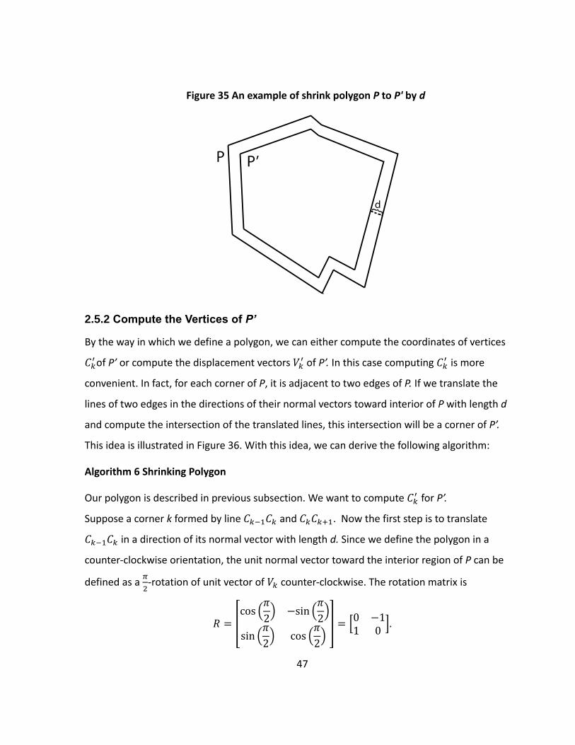
47

Figure 35 An example of shrink polygon P to P' by d

2.5.2 Compute the Vertices of P’

By the way in which we define a polygon, we can either compute the coordinates of vertices

𝐶𝑘′ of P’ or compute the displacement vectors 𝑉𝑘

′ of P’. In this case computing 𝐶𝑘′ is more

convenient. In fact, for each corner of P, it is adjacent to two edges of P. If we translate the

lines of two edges in the directions of their normal vectors toward interior of P with length d

and compute the intersection of the translated lines, this intersection will be a corner of P’.

This idea is illustrated in Figure 36. With this idea, we can derive the following algorithm:

Algorithm 6 Shrinking Polygon

Our polygon is described in previous subsection. We want to compute 𝐶𝑘′ for P’.

Suppose a corner k formed by line 𝐶𝑘−1𝐶𝑘 and 𝐶𝑘𝐶𝑘+1. Now the first step is to translate

𝐶𝑘−1𝐶𝑘 in a direction of its normal vector with length d. Since we define the polygon in a

counter-clockwise orientation, the unit normal vector toward the interior region of P can be

defined as a 𝜋

2-rotation of unit vector of 𝑉𝑘 counter-clockwise. The rotation matrix is

𝑅 = [cos (

𝜋

2) −sin (

𝜋

2)

sin (𝜋

2) cos (

𝜋

2)

] = [0 −11 0

].

48

Figure 36 Intersection of translated edge vector

The desired normal vector with length d can be computed by (See Figure 36)

𝑛𝑘 = 𝑑 ∙ 𝑅𝑉𝑘−1

‖𝑉𝑘−1‖.

The line 𝐶𝑘−1𝐶𝑘 in vector form is

(𝑥, 𝑦) = 𝐶𝑘−1 + 𝑡1 ∙𝑉𝑘−1

‖𝑉𝑘−1‖.

After translation by 𝑛𝑘, the line is (𝑥𝑘 , 𝑦𝑘) = 𝐶𝑘−1 + 𝑛𝑘 + 𝑡1 ∙𝑉𝑘−1

‖𝑉𝑘−1‖.

Then we perform the previous step for line 𝐶𝑘𝐶𝑘+1, the translated line is

(𝑥𝑘+1, 𝑦𝑘+1) = 𝐶𝑘 + 𝑛𝑘+1 + 𝑡2 ∙𝑉𝑘

‖𝑉𝑘‖.

The intersection of (𝑥𝑘, 𝑦𝑘) and (𝑥𝑘+1, 𝑦𝑘+1) is 𝐶𝑘′ which is the coordinate desired (See Figure

36). Setting these two line equations equal, we obtain

𝐶𝑘−1 + 𝑛𝑘 + 𝑡1 ∙𝑉𝑘−1

‖𝑉𝑘−1‖= 𝐶𝑘 + 𝑛𝑘+1 + 𝑡2 ∙

𝑉𝑘

‖𝑉𝑘‖

𝑡1 ∙𝑉𝑘−1

‖𝑉𝑘−1‖− 𝑡2 ∙

𝑉𝑘

‖𝑉𝑘‖= 𝐶𝑘 − 𝐶𝑘−1 + 𝑛𝑘+1 − 𝑛𝑘

(𝑡1, 𝑡2)

[

𝑉𝑘−1

‖𝑉𝑘−1‖

− 𝑉𝑘

‖𝑉𝑘‖]

= 𝐶𝑘 − 𝐶𝑘−1 + 𝑛𝑘+1 − 𝑛𝑘

49

(𝑡1, 𝑡2) = (𝑉𝑘−1 + 𝑛𝑘+1 − 𝑛𝑘)

[

𝑉𝑘−1

‖𝑉𝑘−1‖

− 𝑉𝑘

‖𝑉𝑘‖] −1

.

After we have the pair (𝑡1, 𝑡2), we can substitute it into the line equation for (𝑥𝑘 , 𝑦𝑘) or

(𝑥𝑘+1, 𝑦𝑘+1) to obtain the intersection 𝐶𝑘′ .

Do all the previous steps for 𝑘 = 1 𝑡𝑜 𝑛𝑠, with 𝐶𝑛𝑠+1 = 𝐶0. ∎

Note: The major step in computing 𝐶𝑘′ is solving (𝑡1, 𝑡2). Since above system is 2-by-2, computing

inverse of matrix [

𝑉𝑘−1

‖𝑉𝑘−1‖

− 𝑉𝑘

‖𝑉𝑘‖

] only takes O(1) complexity, which means that computing each 𝐶𝑘′ is

O(1). Since the algorithm compute 𝐶𝑘′ for every vertex, the complexity for Algorithm 6 is O (n),

where n is the number of sides of the polygon.

Figure 37 Shrink Experiment 2 by 0.1

50

We shrunk he polygon in Figure 34 by d=0.1, and then packed same circle set in the shrunken

polygon. The result is shown in Figure 37.

2.6 Summary of the Chapter

In this chapter, we have investigated several algorithms for circle packing. Starting with the simplest

approach, we concluded with a big picture of the algorithm we want. Based on this, the GGL packing

scheme seems to be a perfect choice. We studied, implemented, modified and generalized the GGL

scheme in order to satisfy requirements of our problem. However, the GGL is designed for physical

problem with gravity such as putting bottles into a vertical box. Although the packing provided by

GGL has high packing efficiency, it is not suitable for tubes in a container due to resistance to impact

and flow heat transfer. Then, we developed a new algorithm called the anti-GGL algorithm. we

studied all the concepts of the GGL algorithm such as position number and constraints in a polygon

region, and packed circles with the priority of packing bigger circles in center. Anti-GGL is actually a

combination of the idea in our simple approach and techniques in the GGL. In fact, anti-GGL in

polygonal region is the algorithm we have been using to pack tubes into cross-section areas.

We also develop an algorithm for shrinking polygon to control the distance between packed tubes

and container boundary. Nevertheless, shrinking a polygon is not only meaningful for packing tubes,

but also for design of container shapes. With the shrinking algorithm, we could design containers

with similar cross-sectional shapes, but the details about complicated 3D surface of a container is

beyond the scope of this thesis.

Circle packing is the most important part of our design since a good packing of tubes directly

corresponds to the total volume of the tubular system. It is, however, a start of the whole

design problem. After that, making connections between packed tubes will be another problem.

51

Chapter 3 Preparations for Connection

In this chapter, several definitions and assumptions will be discussed in order to formulate a

method to connect packed tubes in a cross-sectional area. We first define the fundamental

elements for connection. These elements are basically deformed and holed straight tubes. A

feasible tubular network must be able to be decomposed into combinations of finite elements.

Then we will investigate the interference problem between tubes while trying to make a simple

combination of two elements. We have a new definition to quantify how bad the interference

is, and this definition will be an important criterion for making decision of connection. Finally,

we convert the information of packed circles in a cross-section into a graph with all possible

connection. In next two chapters for solving connection problem, the method is based on the

result of this chapter. Thus, this chapter is a transition between tube packing and tube

connection.

3.1 Fundamental Elements

Connection between tubes is not trivial since it is not reasonable to make an arbitrary

connection. In fact, once a tubular network system is produced, some simulations of flow

dynamics and heat transfer are required [5]. Some connections will result complicated dynamic

situations such as turbulence and vortices. Such connections should be avoided since they may

affect the accuracy of simulation. However, sometimes a complicated geometry is required to

make a necessary connection. Thus it is essential to figure out the connections that are

necessary and feasible. The fundamental components of these connections are called elements.

A tubular network system should be constructed by using only finite number of these elements.

In particular, in order to simplify the network and simulation, we should define as few

elements as possible. For an existing connection, it is much better to reduce it to combinations

of existing elements rather than define new elements. In our entire design strategy, we actually

52

need only three fundamental elements. We will also need to introduce a modified element in

future, but it will be introduced in order to solve different problem.

1. I-block element

Figure 38 I-block

As shown on Figure 38, this block is actually a straight tube with same radii at both ends. This

element is required everywhere since it is a tubular network and most of packed tubes are

straight cylinder tubes. The flow and heat transfer are simple for straight tubes with a given

length. Thus, the length is arbitrary.

2. L-block element

Figure 39 L-block

Abstract representation of L-block

Perspective view of L-block

Front view of L-block

Side view of L-block

Abstract representation of I-block

Perspective view of I-block

53

Sometime it is referred as “bend”, a 90-degree bend with same radii on both ends. It can also be

considered as a quarter torus with zero inner radius. This element will be used most frequently

when connecting tubes at the ends of the container.

3. T-block element

Figure 40 T-block

Abstract representation of T-block

Perspective view of T-block

Front view of T-block

Side view of T-block

We also call it “tee”. It is designed for a tube with radius R1 merge to a tube with same radius in

a perpendicular direction. Since the element should be structurally stable, the length of the

tube coming in is R1, and the length of the tube receiving the merging is 2R1. If the tubes are

shorter, the block will not form a complete merging operation.

Since there are not many merging operations in our design, this block is used much less often

than L-block, but it has to be allowed.

54

In this thesis, all network design and tube operations are based on above three fundamental

elements. From their picture, we could see that each element has only one radius. It means that

the above three elements could only connect tubes with same radius. Although it is believed

that connecting tubes with multiple radii would be much harder, we only need one more

element for multiple size tubes. The idea of this new element comes from a fundamental

element of connection. Thus, it is beneficial to discuss the simple case of equal radii before

moving onto the new element.

3.2 End-caps and Interference

Consider the simplest type of connection----connecting two adjacent straight tubes with same

radius at their ends. We can connect them by using two L-blocks facing each other, i.e. a “180-

degree bend”. (See Figure 41)

Figure 41 Endcaps

This connection is usually used at the ends of each cross-section. Therefore, it is called an end-

cap connection. In Figure 41, the blue parts are end-cap connections.

55

It is almost trivial to make one end-cap connection. However, problem arises when making

more than one end-cap connection, especially when their connections are close to each other.

3.2.1 Interference

Consider the case shown in Figure 42, where we have connected tube c1 and tube c2 with end-

caps constructed by two bends. We also have a tube c3 with same radii, which is packed by

anti-GGL scheme tangential to both c1 and c2. We are unable to make any end-cap connection

with c3 since the end-cap of c1 and c2 will block some space enclosed by tube c3 (In Figure 42,

the two line segments tangent to both c1 and c2 define the end-cap, the dashed line is the

space above c3 that is blocked by the end-cap). Since the end-cap interferes with our other

connection, we call this problem interference problem of end-caps. The interference always

exists if we use Algorithm 3 Two Circle Packing Algorithm to place new circles such as the GGL

algorithm and the anti-GGL algorithm. In the packing result of naïve approach, interference will

not occur because Algorithm 3 is not employed.

Figure 42 Interference of end-cap

Note that the interference is not limited to an end-cap between two adjacent circles. In the

right part of Figure 42, we could also see that, an end-cap can be constructed by using two L-

blocks on two tubes and an I-block connecting two L-blocks. This end-cap connects two non-

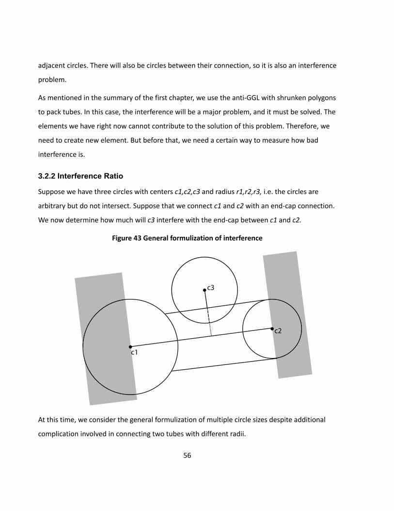
56

adjacent circles. There will also be circles between their connection, so it is also an interference

problem.

As mentioned in the summary of the first chapter, we use the anti-GGL with shrunken polygons

to pack tubes. In this case, the interference will be a major problem, and it must be solved. The

elements we have right now cannot contribute to the solution of this problem. Therefore, we

need to create new element. But before that, we need a certain way to measure how bad

interference is.

3.2.2 Interference Ratio

Suppose we have three circles with centers c1,c2,c3 and radius r1,r2,r3, i.e. the circles are

arbitrary but do not intersect. Suppose that we connect c1 and c2 with an end-cap connection.

We now determine how much will c3 interfere with the end-cap between c1 and c2.

Figure 43 General formulization of interference

At this time, we consider the general formulization of multiple circle sizes despite additional

complication involved in connecting two tubes with different radii.

57

From Figure 43, we see that the actual part of c3 that interfere with the end-cap between c1

and c2 is characterized by the the dashed line. In order to avoid interference, the dotted line in

Figure 43 is the maximum allowable radius of the narrowest part of the end-cap. Thus, we

define the interference ratio of c1, c2 w.r.t to c3 is

𝑖𝑛𝑡𝑒𝑟𝑓𝑒𝑟𝑒𝑛𝑐𝑒 𝑟𝑎𝑡𝑖𝑜 = 𝛾 =𝑙𝑒𝑛𝑔𝑡ℎ 𝑜𝑓 𝑑𝑜𝑡𝑡𝑒𝑑 𝑙𝑖𝑛𝑒

min{𝑟1, 𝑟2}.

The key part of computing 𝛾 is to compute the length of dotted line.

In fact, 𝑙𝑒𝑛𝑔𝑡ℎ 𝑜𝑓 𝑑𝑜𝑡 𝑙𝑖𝑛𝑒 = (𝑑𝑖𝑠𝑡𝑎𝑛𝑐𝑒 𝑓𝑟𝑜𝑚 𝑐3 𝑡𝑜 𝑙𝑖𝑛𝑒 𝑐1𝑐2) − 𝑟3.

Note that the above case will only happen if center c3 is in the white area in Figure 43. If c3 is in

the shadowed area in Figure 43, it will not interfere with the end-cap of c1 and c2. This can be

easily checked by computing ∠𝑐3𝑐1𝑐2 and ∠𝑐3𝑐2𝑐1 using cosine law in △ 𝑐1𝑐2𝑐3. If any of

∠𝑐3𝑐1𝑐2 or∠𝑐3𝑐2𝑐1 is greater or equal to 90 degree, c3 is in the shadowed area.

Now we suppose c3 is in the white area. The distance from c3 to line c1c2 is actually the height

of △ 𝑐1𝑐2𝑐3 over edge c1c2. We can compute the area of △ 𝑐1𝑐2𝑐3 by Helen’s formula:

𝑎𝑟𝑒𝑎 𝑜𝑓 △ 𝑐1𝑐2𝑐3 = √𝑝(𝑝 − |𝑐1𝑐2|)(𝑝 − |𝑐2𝑐3|)(𝑝 − |𝑐1𝑐3|),

𝑤ℎ𝑒𝑟𝑒 𝑝 =|𝑐1𝑐2| + |𝑐2𝑐3| + |𝑐1𝑐3|

2

Also,

𝑎𝑟𝑒𝑎 𝑜𝑓 △ 𝑐1𝑐2𝑐3 =1

2|𝑐1𝑐2| ∙ (ℎ𝑒𝑖𝑔ℎ𝑡 𝑜𝑓 𝑐1𝑐2)

Equating the right hand side, we may solve for the height of c1c2,

ℎ𝑒𝑖𝑔ℎ𝑡 𝑜𝑓 𝑐1𝑐2 = 𝑑𝑖𝑠𝑡𝑎𝑛𝑐𝑒 𝑓𝑟𝑜𝑚 𝑐3 𝑡𝑜 𝑙𝑖𝑛𝑒 𝑐1𝑐2 =2√𝑝(𝑝 − |𝑐1𝑐2|)(𝑝 − |𝑐2𝑐3|)(𝑝 − |𝑐1𝑐3|)

|𝑐1𝑐2|

so that

58

𝛾 =

2√𝑝(𝑝 − |𝑐1𝑐2|)(𝑝 − |𝑐2𝑐3|)(𝑝 − |𝑐1𝑐3|)|𝑐1𝑐2|

− 𝑟3

min{𝑟1, 𝑟2}

From the above formula, we see that if 𝛾 ≤ 0, circle c3 will block the line segment between c1

and c2, and c1 and c2 will never be connected. This is the easy case. We will now discuss the case

𝛾 > 0.

3.2.3 Interference Tolerance

Now we apply 𝛾 as a criterion in our packed tubes. Assume that 𝛾 > 0, since 𝛾 ≤ 0 is trivial.

From the definition of 𝛾, if 𝛾 ≥ 1, there will be no interference between c1 and c2. Therefore,

the tricky case is when 0 < 𝛾 < 1, and our discussion focus on this situation. Due to the

placement of a new circle in anti-GGL, most of our packing is “triangular packing”, i.e. left case

in Figure 42, three circles with same radii tangent to each other. Despite of interference, this

connection has to be allowed because most of circles placed by anti-GGL are in this form. In

fact, 𝛾 = 0.7321 for this triangular packing, and it is very fundamental. Based on the formula in

previous subsection, the smaller 𝛾 indicates a larger interference. All pairs of circles for which

𝛾 ≥ 0.7321 are eligible for connecting since the interference is better that the fundamental

case. In practical, we may need this condition to be weaker, i.e. we will allow some connections

with smaller 𝛾. Therefore, we could set a tolerance 𝜸 denoted by 𝛾𝑡𝑜𝑙, and we could connect all

pairs of tubes with 𝛾 ≥ 𝛾𝑡𝑜𝑙 to be connected.

Note that 𝛾𝑡𝑜𝑙 is not trivial or arbitrary. It cannot be greater than the fundamental case. In our

standard problem, the range for choosing 𝛾𝑡𝑜𝑙 is 0 < 𝛾𝑡𝑜𝑙 ≤ 0.7071 < 0.7321. We will explain

why 0.7071 is the upper bound of 𝛾𝑡𝑜𝑙 in the next two subsections.

3.2.4 Approaches to Interference

Based on the argument in previous subsections, we actually want to ensure that connection

have “good”, i.e. high 𝛾, interference. For bad interference, i.e. 𝛾 < 𝛾𝑡𝑜𝑙, we do not want to

make any connection at all. Since the elements defined in subsection 3.1 is not adequate for

59

this problem, we need to define new elements for solving interference. However, when

introducing the new element, the following principles should be considered:

1. The geometry of the elements should be simple. This principle is for convenience of

simulation. An element such as an X-block is not allowed anywhere.

2. Introducing elements as less as possible. If we really need more than one element, it is

better if they have similar geometrical shapes.

3. The elements should be smooth. The elements should not have any sharp edge. This is

most concerned because flow near sharp edges can be very complicated.

4. The elements can be used in other cases.

5. Loss of volume is minimized. Solving the interference problem involves shrinking the

end-caps. In our design problem, maximizing the volume of the tubular system is the

top priority. Shrinking end-cap would result in some volume lose, and we want the lost

volume to be minimum.

Using above five principles, we can try to determine how good an interference solution is. The

first approach to our interference problem is the narrowed end-cap shown on Figure 44.

Figure 44 Narrowed end-cap

Figure 45 Bend with two radius

Is this solution good? We can check our five principles. The elements we introduce are (i). a

straight tube with changing diameters. (ii). a bend with non-zero inner radius. They are simple,

but the introduced elements can only be used in this case. Almost everything can be

60

implemented without these two element. The worst part for this solution is that it loses too

much volume. Half of the volume of end-cap is wasted in the thin bends connecting two tubes.

As a result, this solution is neither the best nor the worst. It is just a naive approach to shrink

the end-cap.

Now, it is time to bring back to our original elements from subsection 3.1. If we create a new

element by modifying some fundamental elements, this element would definitely satisfy all

five principles except principle 4. A natural idea is to modify the bend, i.e. the L-block. As

shown on Figure 45, if we allow the two ends of bend to have different radii and one moves

from the center of one circle to the center of the other circle in an elliptical path, we have

produced a more satisfactory shrunken end-cap.

3.2.5 The New Element: Modified L-block

From the above idea in Figure 45, we create this new element, called a modified L- block.

Assume if that R2<R1, some views of the modified L-block are shown below:

Figure 46 Modified L-block

Abstract representation

Perspective view

Front view

Side View

61

Very fortunately, we can generate a more beautiful representation of the geometry of this

element. Note that the 3D model tool for drawing this element is different from previous

elements. The 3D models of elements in section 3.1 were created by SoildWorks. However,

the 3D representation of modified L-block shown above was produced using Mathematica.

Mathematica allows one to work with mathematical parameterization for the surface of

modified L-block. The formula of the parameterization is

x(θ, ϕ) =𝑅1𝑅2(1 + 𝑐𝑜𝑠𝜃)𝑐𝑜𝑠𝜙

√𝑅12 cos2 𝜙 + 𝑅22 sin2 𝜙,

y(θ, ϕ) =𝑅1𝑅2(1 + 𝑐𝑜𝑠𝜃)𝑠𝑖𝑛𝜙

√𝑅12 cos2 𝜙 + 𝑅22 sin2 𝜙,

z(θ, ϕ) =𝑅1𝑅2𝑠𝑖𝑛𝜃

√𝑅12 cos2 𝜙 + 𝑅22 sin2 𝜙.

𝑊ℎ𝑒𝑟𝑒 𝜃 ∈ [0,2𝜋], 𝜙 ∈ [0,𝜋

2] , 𝑅1 𝑎𝑛𝑑 𝑅2 𝑎𝑟𝑒 𝑡ℎ𝑒 𝑡𝑤𝑜 𝑟𝑎𝑑𝑖𝑖 𝑜𝑓 𝑐𝑖𝑟𝑐𝑙𝑒𝑠 𝑎𝑡 𝑡ℎ𝑒 𝑒𝑛𝑑𝑠.

A derivation of the above formula is presented in Appendix A.

The range of 𝜙 ∈ [0,𝜋

2] will only yield a single element, a 90-degree bend. If we choose 𝜙 ∈

[𝜋

2,3𝜋

2], the result is an end-cap with connecting two tubes with radius R1 but with a radius

R2<R1 between them, as shown in Figure 47.

Figure 47 End-cap of Modified L-block

This is exactly what we need. In ultimate design problem, we packing shall be tubes with three

radii i.e. 𝑅1 = √2𝑅2 = 2𝑅3. We can choose the radii of two ends of a modified L-block to be

62

𝑅1 = 𝑅1, 𝑅2 = 𝑅2. The R2 corresponds to the dotted line in Figure 43. The interference ratio in

this case is

𝛾 =𝑅2

𝑅1=

𝑅2

𝑅1=

1

√2= 0.7071

The nice thing is that 0.7071 < 0.7321, which means that it works in the “triangular packing”

case. This is the reason why choosing 0.7071 as the upper bound of 𝛾𝑡𝑜𝑙 in subsection 3.2.3.

One advantage of defining the modified L-block in this way is that it can be used in other

connections, for example, connecting two tubes with different radii, i.e. 𝑅1 = √2𝑅2 in our

standard problem. In Figure 48, two tubes with different radii are connected by an end-cap

constructed by a L-block and a modified L-block.

Figure 48 End-cap of two tubes with different radii

This element was introduced in order to solve the interference problem, but it seems to

provide a practical way of connecting tubes with two different radii. In conclusion, the

modified L-block element comes from our original fundamental element, so it is simple,

smooth and efficient. However, by choosing some specific radii for the element, it can also be

used in other connections such as end-cap connections between two different tubes. It

satisfies all five principles for defining a new element, and thus it is a perfect new element.

3.3 Graph Representation for Possible Connection

Now with a complete list of elements and interference ratios, we can decide which pairs of

tubes are eligible to be connected. Once we have determined all possible connection, we need

to construct a mathematical representation that could represent the relationship of possibility

of connection. Graph provides a good mathematical representation.

63

Definition 2 Graph [10] A graph G=(V, E) consists two sets V and E

The elements in V are called vertices.

The elements in E are called edges.

Each edge has a set of one or two vertices associated to it, which are called endpoints. An

edge is said to join its endpoints.

For our problem, we construct a graph by setting the set of centers of tubes as the vertices V

and adding connecting two vertices with an edge if the corresponding tubes can be connected.

Note that such a graph is constructed at every cross-section of packed tube. At first, we need

to initialize an interference tolerance 𝛾𝑡𝑜𝑙 > 0. Any two tubes with interference ratio greater

than 𝛾𝑡𝑜𝑙 will not be connected so that their corresponding vertices will not form an edge in

the graph. The algorithm is described by mean of pseudocode:

Algorithm 7 Constructing Connection Graph

Input: n Packed tubes/circles with centers (c1,c2,…cn). 𝛾𝑡𝑜𝑙 > 0, interference tolerance.

Output: Graph G with edges that define all possible connections

Initialization: Graph G=(V, E), V=(c1,c2,…cn), i.e. centers of packed tubes. 𝐸 = ∅

for circle i =1:n

for circle j=(i+1):n

if line segment ci-cj intersects with polygon boundary (Algorithm 5)

continue

else

compute

𝛾 = 𝑚𝑖𝑛{𝑖𝑛𝑡𝑒𝑟𝑓𝑒𝑟𝑒𝑛𝑐𝑒 𝑟𝑎𝑡𝑖𝑜 𝑜𝑓 𝑖 𝑎𝑛𝑑 𝑗 𝑤. 𝑟. 𝑡 𝑎𝑙𝑙 𝑜𝑡ℎ𝑒𝑟 𝑡𝑢𝑏𝑒𝑠}

if 𝛾 ≥ 𝛾𝑡𝑜𝑙

add edge (ci,cj) to graph G

else

continue

endfor

endfor

Output graph G after all iterations are finished. ∎

64

This algorithm basically checks all possible pairs of connections. The good news is that both

Algorithm 5 and computing interference ratio are O(1). The bad news is that the running time

of this algorithm is not better than the GGL packing algorithm. In fact, it takes n(n-1)

operations to check all possible pairs of tubes. Also for each pair, computing the minimum of

interference ratio of the pair w.r.t all other tubes in the packing set takes (the operations of

computing one interference ratio)*(n-2); since the first part is O(1), the complexity of this part

is O(n-2). The complexity for the whole algorithm is O(n(n-1)(n-2))=𝑂(𝑛3).

A visual example of one output with corresponding packed circles is shown on Figure 49. It is

created by Matgraph---a plugin of Matlab for graph theory [18].

Figure 49 An example of connection graph

In this figure, we choose 𝛾𝑡𝑜𝑙 = 0.7071. Green dots are the vertices of connection graph G. The

blue lines are the edges of G, which define possible connections. In this case, we could see that

some edges cross each other; thus these crossing edges cannot be chosen as connection at the

same time. In our Matlab implementation, we output another list which contains all crossing

edges; Every time when we make connection decisions, we will inspect this list to see if there are

any conflicts. Algorithm 7 can be significantly improved to linear complexity. In fact, it is not

0 0.2 0.4 0.6 0.8 1 1.2 1.4 1.6 1.8 2

1.2

1.4

1.6

1.8

2

2.2

2.4

2.6

65

necessary to check all pairs of tubes. We do not want to connect two tubes that are too far away

from each other. For each tube, we consider connecting it with the tubes within some

neighborhood of it. In this case, we can use information from our anti-GGL packing scheme to

construct a neighborhood with fixed radius for each tube. We need only to check possible

connections within this region. The data structure of this improvement needs to use the idea of

adjacent list; detail for this improvement and complexity analysis can be found in the Appendix B.

However, this improvement requires information from a sequential packing algorithm such as

anti-GGL packing scheme, which means that it has to be built into the packing algorithm

program. If the packing algorithm is not GGL or anti-GGL, this improvement may not be better

than Algorithm 7. Therefore, since this improvement does not work for given arbitrary packing, it

is not implemented in our case.

3.4 Moving towards the Connection Problem

The output of Algorithm 7, graph G, is the final result of this chapter. In the next two sections,

we will discuss algorithms for choosing connections at one cross-section. These algorithms are

classical discrete optimization algorithms, and they will be performed on our connection graph

G. The edges selected by these algorithms as solutions define connections that we decide to

make. Details about what kinds of connections we want and how these algorithms work will

not be discussed here, but since G is sparse, there will be some tricks involved in these

algorithms.

Moreover, in this chapter, we have defined the fundamental elements: I-block, L-block, T-block

and modified L-block. In Chapter 5, we will use these elements to construct operations on

tubes at different cross-sections. Based on these elements, we shall illustrate what operations

we allowed and what operations are disallowed.

In conclusion, this chapter provides all the background information as well as connection graph

G constructed from packed circles for making decisions about connecting. It is a transition

66

between our circle packing problems and connecting problems. Although this chapter is non-

technical, it is still fundamental and essential.

67

Chapter 4 One-Path Network and Travelling Salesman

Problem (TSP)

Designing a tubular network system by connecting tubes in regions with varying cross-sections

is a generally difficult problem. In this chapter, we will investigate this problem by starting with

the construction the simplest tubular network system---the one-path network system. This

system is designed for packed tubes in a container with non-varying cross-sections (like the

barbeque pool heater), so the container in this chapter has two identical ends.

Although this system is the simplest, the connection problem for designing such system is non-

trivial. In fact, we will reduce the connection problem in this case as a classical combinatorial

optimization problem called the travelling salesman problem (or TSP) with the connection graph G

defined in last chapter. The TSP problem is NP-Complete, so there is no polynomial-time algorithm

that can generally solve this problem. However, it does not mean that TSP cannot be solved in

some special cases. As we concluded in last chapter, our connection graph G is sparse and

Euclidian. Therefore, we can play some tricks when we choose our algorithm for TSP.

4.1 One-Path Network System

Before we continue with the details of our problem, several clarifications and assumptions are

necessary. Suppose we have a prism container with longitudinal symmetry, i.e. non-varying cross-

section and identical ends. We also have tubes packed in the cross-sections of the container.

Because of the longitudinal symmetry, the packed tubes are straight tubes and the packed circles

in the front end and rear end are same. Thus, the connection graphs for packing in front end and

rear end are also same; we denote this graph by G for both ends. Actually, in this chapter, we will

apply our algorithm on one graph for two ends since they have identical connection graphs.

Now we can define the one-path network system. We choose a tube as inlet and another tube

as outlet, and we make connections between all tubes. If the connected tubes form one long

tube, this system is called a one-path network system. Moreover, the inlet and outlet of our

68

system should be same as the ones we choose. An example of one-path network system is

presented in Figure 50.

Figure 50 Small example of one-path system

In Figure 50 (a), 5 circles are packed into the region of rectangle. On (b), it can be seen that the

packing is identical at two ends. We choose tube 1 as inlet and tube 5 as outlet, and then we

connect 1 to 2, 2 to 3, 3 to 4 and 4 to 5. This connection forms a long tube with 1 as inlet and 5

as outlet. In this case, the inlet and outlet are on different ends. It seems to be trivial, but this

example only illustrates the concept of one-path system. It does not show any complexity of the

system. In fact, the connection graph in Figure 50 is the simplest graph called path. However,

from this example, we can conclude some characteristic of one-path system.

The one-path system contains no T-blocks. A T-block produces bifurcation in the network. A

long tube has no bifurcation.

All tubes are connected. Every tube in the packing except the inlet and outlet are

connected by two end-caps, one end-cap at each end. No tube will be left alone without

being connected to other one.

69

The locations of inlets and outlet depends on the number of packed tubes. If the number

of packed tubes is odd, i.e. 5 in Figure 50, the inlet and outlet are situated on different

side. Otherwise, they are on the same side.

As a result, we have a big picture of what connections we want to pick. If we have chosen the

inlet and outlet, we want a connection that visits every tube exactly once at each end in

alternating order. Since we have one connection graph for both ends, that is equivalent to pick

edges in G that these edges visit every vertex in G. Note that edges G contains all possibility of

connections for both ends. Thus, edges picked as connections should visit every vertex exactly

once for the inlet and outlet vertices and twice for all other vertices. Now the question is that: Is

there any concept in graph theory that dealing with the visitation of every vertex? The answer is

yes; it is the concept of a Hamiltonian cycle.

4.1.1 Hamiltonian Cycle

Definition 3 [10] Walk. A walk in a graph G is an alternating sequence of vertices and edges:

𝑊 = 𝑣0, 𝑒1, 𝑣1, 𝑒2, … , 𝑒𝑛, 𝑣𝑛

such that for j=1,…,n, the vertices 𝑣𝑗−1and 𝑣𝑗 and end-points of 𝑒𝑗

Definition 4 [10] Path. A path is a walk with no repeating edges or vertices.

Definition 5 [10] Cycle. A cycle is a path with 𝑣0 = 𝑣𝑛.

With all above definitions, we can define a Hamiltonian cycle.

Definition 6 [10] Hamiltonian Cycle. A Hamiltonian cycle of graph G is a cycle that visits

each vertex of G exactly once.

An example of a Hamiltonian cycle in a connection graph G is shown on Figure 51 which is the

connection graph of packing of big circles in Figure 34. The red lines comprise the cycle. Finding a

Hamiltonian cycle is a classical problem in combinatorial optimization. It is NP-complete, so there

is no deterministic polynomial time algorithm to solve it. The best known deterministic algorithm

is dynamical programming which has a run time of 𝑂(𝑛22𝑛) [20]. It is a little better than

70

enumerating all possible cycles which is 𝑂(𝑛!), but it is still infeasible for graphs with more than

30 vertices. Therefore, we need to consider non-deterministic algorithms.

Figure 51 Hamiltonian cycle in a connection graph

Moreover, in our system, we do not want a long closed tube. We want a long tube with a

chosen inlet and a chosen outlet. Therefore, instead of cycle, path is a more useful instance for

our problem. Similar to Hamiltonian cycle, a Hamiltonian path of graph G is a path from a

vertex to another vertex that visits each vertex of G exactly once. If we set the start vertex as

the inlet and end vertex as outlet, a Hamiltonian path between them will correspond to a one

long tube between the inlet and outlet.

4.1.2 Corresponding Hamiltonian Path to a One-path Network System

This subsection perhaps is the key of this chapter.

Figure 52 shows how a Hamiltonian path in G corresponds to a one-path network in cube

container. Several explanations are required.

71

Figure 52 Relation between Hamiltonian path and a one-path network system

In this Figure 52, 9 tubes are packed in a cube container with a square cross-section. Obviously,

the packing is neither GGL nor anti-GGL. It looks like the naïve approach, but it does not matter

because this is enough to illustrate the idea. The left diagram in Figure 52 is the packing and

the connecting graph G. Both blue and red lines are edges in G. The red lines are the edges

chosen to define the Hamiltonian path starting from tube 1 to tube 9. As shown in the right

diagram in Figure 52, tube 1 is the inlet of the system and tube 9 is its outlet. The right part is

the 3D representation of the packed tubes with connection. The red arcs represent the end-

cap connections that correspond to the red edges in left part. The red dotted line indicates

that the end-cap is on the front side of the container, and the red dashed line indicates that

the end-cap is on the rear side of the container. This description also applies in the left

diagram. As a result, we can make the following conclusion:

1. The edges in the paths are end-cap connections between two endpoints of the edge.

2. The inlet and outlet are the, respectively, start vertex and end vertex of the path.

3. If an edge is in the odd position of the path, the corresponding end-cap is on the rear

side of the container. If an edge is in the even position of the path, the corresponding

end-cap is on the front side of the container.

72

4. Since the path visits every tube exactly once, each tube except inlet and outlet are

connected alternately on the front side exactly once and on the rear side exactly

once.

Thus, the connection of the Hamiltonian path forms a system composed of one long tube.

4.1.3 Weighted Hamiltonian Path

Now we have the relation between a Hamiltonian path and corresponding connections. The

problem is how to find such a path. From our discussion of Hamiltonian cycles we know that to

find a Hamiltonian path is not easier than to find a Hamiltonian cycle. Therefore, enumerating

all such path and find the one we want is not feasible. In fact, we do not want all Hamiltonian

paths. We just want the “best” one among all paths. Although the “best” is not defined here,

we can still give an abstract representation of it.

Suppose we have a graph G=(V,E) such that for each edge 𝑒 ∈ 𝐸, we have a weight 𝑤𝑒. For each

Hamiltonian path in the graph, we sum the weights of the edges which comprise the path. The

best Hamiltonian path will have the maximum or minimum sum among all Hamiltonian paths. This

problem is called the weighted Hamiltonian path problem.

In our connection graph, the weights 𝑤𝑒 still remain unclear. They could be the Euclid distances

between two vertices or some factor where depends on the interference ratio. However, since

the 𝑤𝑒 are considered to be arbitrary, we will focus on solving the weighted Hamiltonian path

problem rather than how weights are defined.

Although the weighted Hamiltonian path problem is not famous, its brother --- weighted

Hamiltonian cycle problem --- is a classical and well studied problem in combinatorial

optimization. The other widely used name for weighted Hamiltonian cycle problem is the

travelling salesman problem or TSP in abbreviation. This problem was first discussed in the 19th

century as follows: A salesman wants to travel to several cities, visiting each city only once, and

come back to the starting city with the shortest tour length [27]. Much research has been done

on this problem since the 20th century. Now there is even an App from App Store on iPhone could

solve small TSP [35]. However, the best deterministic algorithm for TSP is still based on dynamic

73

programming. It has a complexity of 𝑂(𝑛22𝑛) and has not been improved for 50 years [20]. For

our problem, we want the TSP path instead of TSP cycle. In next subsection, we will show that

solving TSPP (TSP path) is equivalent to solving TSP cycle. We assume that we shall minimize our

total weight on the path in all instances of TSP.

4.1.4 TSPP≡𝒑TSP

In order to prove the TSP path problem is equivalent to the TSP cycle problem, we need to

assume that we can solve TSPP first, we solve a particular TSP by calling the solver of TSPP a

polynomial number of times. This process is called computational reduction. In this case, we

say TSP reduces to TSPP, denoted by TSP≤𝑝TSPP. If we can prove that TSPP can also reduce to

TSP denoted by TSPP≤𝑝TSP, we can conclude that TSPP is polynomially computationally

equivalent to TSP, denoted by TSPP≡𝑝TSP.

Proof: TSP≤𝑝TSPP

Since a cycle is a special case of a path, we could set the starting vertex and ending

vertex in the TSPP to be the same. Once we run this TSPP, it will provide a cycle which is

the solution of the TSP. This part is trivial.

TSPP≤𝑝TSP

Suppose that we have a graph G=(V, E), with weight 𝑤𝑒 𝑓𝑜𝑟 𝑒 ∈ 𝐸 and a TSP solver. If

we want to solve the TSPP between two vertices v and u of V. we can do the following:

We add a new edge between u and v with a weight of negative infinity weight. If the

edge uv already exists, we replace its weight with negative infinity. This will not affect

the TSPP because the TSPP between u and v will never use the edge between them. In

practice, we cannot implement negative infinity; we will set this weight to be the

negative of the summation of all weights in E. In other words, the absolute value of this

weights must be greater than any cycle in the graph. We denote this new graph by G’.

74

If we run a TSP solver on G’, the edge uv will be chosen in the TSP tour. To see this,

suppose the negative, the TSP solution does not contain this edge. Let the TSP solution

be denoted by T and 𝑤(𝑇) the sum of the weights of all the edges in T. For any tour T’

using uv, we have

𝑤(𝑇) ≤ 𝑤(𝑇′) = 𝑤𝑢𝑣 + 𝑤(𝑃𝑎𝑡ℎ 𝑓𝑟𝑜𝑚 𝑢 𝑡𝑜 𝑣 𝑣𝑖𝑠𝑖𝑡𝑠 𝑎𝑙𝑙 𝑜𝑡ℎ𝑒𝑟 𝑣𝑒𝑟𝑡𝑒𝑥).

This is true by our assumption that T is a TSP tour, we rewrite it as follows:

𝑤(𝑇) − 𝑤(𝑃𝑎𝑡ℎ 𝑓𝑟𝑜𝑚 𝑢 𝑡𝑜 𝑣 𝑣𝑖𝑠𝑖𝑡𝑠 𝑎𝑙𝑙 𝑜𝑡ℎ𝑒𝑟 𝑣𝑒𝑟𝑡𝑖𝑐𝑒𝑠) ≤ 𝑤𝑢𝑣.

Recall, however, that we set that 𝑤𝑢𝑣 to be smaller than the negative of the summation

of all weights. Therefore, it cannot be greater than the left hand side. We have arrived

at contradiction

Therefore, the TSP tour in G’ must contain uv. Moreover, the path from u to v which

visits all other vertices corresponds to the TSPP in G. It is clear that this path is the TSPP

in G’. If there is another such path that is smaller than this path, it will be in our TSP

tour of G’. Since the only difference between G and G’ is the edge uv and the TSPP in G’

does not contain uv, it is also the TSPP in G from u to v.

As a result, we have solved the TSPP in G by calling the TSP solver polynomial times,

thus we prove the theorem ∎

4.1.5 From Practical to Abstract

Now we can reverse the logical order of this section: We know that TSP is polynimially

equivalent to TSPP, and TSPP is a Hamiltonian path. By the argument of first two subsections, a

Hamiltonian path in a connection graph corresponds to a one-path network system in a prism

container. Following this process, we can reduce the one-path network system design to a TSP

in connection graph G of the packed tubes if we choose appropriate weights for each edge in G.

Although weights of connections still remain unclear, it does not affect the fact that researching

75

TSP is beneficial. In the rest of this chapter, we will focus on mathematical technique of solving

TSP in the connection graph G despite any practical aspects of design problems.

4.2 Subtour Elimination with Branch and Cut Algorithm for TSP

[14][15]

As TSP is a well-studied problem in combinatorial optimization, many approaches have been

developed, including deterministic algorithms such as dynamical programming (𝑂(𝑛22𝑛)) [20]

and enumerating all tours (𝑂(𝑛!)). A remarkable aspect of tours in TSP is that the minimum

spanning tree (MST) [22] is the lower bound of TSP [27]. Thus, we can enumerate tours by

starting with an MST. This action can improve the feasibility of enumerating up to a graph with

thirty vertices, but it is already the end of the deterministic algorithm. Later, some

approximation algorithms for TSP cames out. The most famous algorithm is Christofides

algorithm [19]. It is a 3

2-approximate algorithm which means that the solution provided by this

algorithm is not greater than 1.5 times that of optimal TSP. However, the output of this

algorithm is almost near 1.5 of optimal TSP. Moreover, it requires that the weights of edges

satisfy the triangle inequality. Since at this point, we want the weights to be arbitrary, this

algorithm is not considered here even though it is still the best approximation algorithm for

TSP at present.

Based on the above facts, we need to consider non-deterministic algorithms. These algorithms

do not guarantee an optimal solution or termination. A typical non-deterministic algorithm is

the nearest neighbor Heuristic Algorithm [19]. There is absolutely no control over the quality of

its result. Another non-deterministic algorithm is the Genetic Algorithm [16], but the

implementation of full genetic algorithm is complicated. Connection graphs G in our tubular

network problem are sparse, i.e. there are not too many edges. Therefore, a desirable algorithm

should exploit, at least to some degrees, the sparseness of G, and the implementation is not too

difficult. Finally, we decide to use subtour elimination with branch and cut algorithm [15]for our

76

TSP in connection graph. This algorithm is based on integer programming, and it is a non-

deterministic algorithm that may not terminate.

4.2.1 Characteristic Vector and Integer Programming

Given a graph, G=(V,E), with weights 𝑤𝑒, such that for each edge 𝑒 ∈ 𝐸, we define the

following variables

𝑥𝑒 = {1, 𝑖𝑓 𝑒 𝑖𝑛 𝑐ℎ𝑜𝑠𝑒𝑛 𝑖𝑛 𝑇𝑆𝑃 𝑡𝑜𝑢𝑟0, 𝑜𝑡ℎ𝑒𝑟𝑤𝑖𝑠𝑒

𝑥𝑒 is called the characteristic variable of edge e. The vector 𝑥 = (𝑥1, 𝑥2 …𝑥|𝐸|) with dimension

|E| is called the characteristic vector of G.

For each vertex 𝑣 ∈ 𝑉, in order to form a tour, exactly two edges of each vertex must be

chosen in the TSP. Thus, the sum of the characteristic variables of all edges incident to v is

equal to 2. We denote the set of all edges incident to v as 𝛿(𝑣). We have the following integer

programming (in short IP) problem for the TSP:

min∑ 𝑤𝑒𝑥𝑒

|𝐸|

𝑖=1

s.t.

∑(𝑥𝑒 , 𝑒 ∈ 𝛿(𝑣)) = 2, 𝑓𝑜𝑟 𝑎𝑙𝑙 𝑣 ∈ 𝑉 ,

𝑥𝑒 ∈ {0,1}, 𝑓𝑜𝑟 𝑎𝑙𝑙 𝑒 ∈ 𝐸.

The IP problem is also NP-hard. Therefore, trying to solve the TSP by solving the above IP is still

infeasible. However, this mathematical formulation of TSP provides a greater opportunity to

study the problem in depth. We can start dealing with the IP by assuming x is not integer.

4.2.2 Linear Programming Relaxation

Since the above IP problem is a 0-1 IP, i.e. the choice for variables is either 0 or 1, we can allow

the variables to be a fractional between 0 and 1. We just need to change the constraints 𝑥𝑒 ∈

{0,1} into 0 ≤ 𝑥𝑒 ≤ 1. In this way, the IP becomes a linear programming. This procedure is

called linear programming relaxation.

77

This linear programming problem is called relaxed linear programming in short RLP. (See

below.) If we solve this RLP by simplex or interior point methods, we shall see below the

solution x may not be the solution we want.

Relaxed linear programming of TSP


|𝐸|

𝑖=1

s.t.

∑(𝑥𝑒 , 𝑒 ∈ 𝛿(𝑣)) = 2, 𝑓𝑜𝑟 𝑎𝑙𝑙 𝑣 ∈ 𝑉 ,

0 ≤ 𝑥𝑒 ≤ 1, 𝑓𝑜𝑟 𝑎𝑙𝑙 𝑒 ∈ 𝐸.

Most of the time, the solution of the above RLP is fractional, and a fractional solution cannot

correspond to a tour in G. It is, however, possible the solution of above RLP is integer. However,

if even the solution is an integer vector, it may not correspond to a TSP tour (See Figure 53). If

we take a close look at this kind of solution in the graph G (As in Figure 53), we could see some

pattern of this solution

Figure 53 Subtour of an integer solution

Figure 54 Difference of TSP and subtour

The corresponding edges of the RLP solution are red lines in Figure 53. The solution is integral

and satisfies all constraints in original IP. However, it is not a TSP tour. It contains several small

cycles; we call these cycles subtours. In fact, a solution with subtours does not violate the

78

constraints in the IP of TSP. In order to get rid of subtours in our RLP solution, we need to

understand the difference between subtours and TSP tours.

4.2.3 Difference between Subtour and TSP Tour

We need the following definition to understand the difference:

Definition 7 Cut. [27] In a graph G=(V, E), a cut of vertices subset 𝐴 ⊆ 𝑉, is a set of edges

such that one end point is in A and another is not in A, denoted by 𝛿(𝐴). Note that 𝛿(𝑣)

for 𝑣 ∈ 𝑉 is the set of all edges that are adjacent to 𝑣.

Definition 8 Connected. [27] A graph is connected if and only if there is a walk between each

pair of vertices.

Definition 9 Component. [27] A component is a subgraph H such that no subgraphs of G

that contain H is connected. Note that a component is always connected.

Since a TSP tour is a cycle that visits every vertex, each edge in the tour has to intersect the cut

of each subset of V at least twice.(See Figure 54.) We can formulate this argument as a

constraint in IP as follows:

∑(𝑥𝑒 , 𝑒 ∈ 𝛿(𝑆)) ≥ 2, 𝑓𝑜𝑟 𝑒𝑣𝑒𝑟𝑦 𝑆 ⊆ 𝑉. (∗)

On the other hand, the subtour solution such as the one in Figure 53 will have components.

The cuts of these components have no intersections with the edges in the tour. As a result, a

RLP solution with subtours will violate the above inequality for some subset 𝑆 ⊆ 𝑉.

Therefore, the differences between TSP tours and subtours are given in the above inequalities.

However, since these inequalities are generated for all subsets of V, there are 2|𝑉| many

inequalities. It is not practical to add all of them to our IP. In fact, not all of these constraints

are violated by the subtour solution. This fact brings up the idea of “cutting plane”.

4.2.4 Cutting Plane Method [14]

The main idea of the cutting plane method is “only add the constraints that are necessary”. We

only need the constraints of the vertex subsets whose cuts contains at most one edge from our

subtour solution. In the last subsection, we have observed that each component in subtour

79

solution has no edges intersecting with the subtour solution. We can use this fact as our cutting

plane.

We construct a new graph G*= (V*, E*) from G=(V,E) using the following strategy:

V*=V. If 𝑥𝑒 ≥ 0, then 𝑒 ∈ 𝐸∗. Otherwise, 𝑒 ∉ 𝐸∗.

In other words, G* is the subgraph of G with same vertex set V and edges in E with a non-zero

RLP solution. G* is called a LP graph of G.

Therefore, if there are subtours in our RLP solution, G* will not be connected. Moreover, each

component in G* corresponds to a subtour in the RLP solution. We just need to use a depth-

first search to find all components of G*, say 𝑆1, 𝑆2 …𝑆𝑚. The cuts of 𝑆1, 𝑆2 …𝑆𝑚 violate (∗) in

4.2.3. We can add the following constraints, called subtour inequalities, to our IP:

∑(𝑥𝑒 , 𝑒 ∈ 𝛿(𝑆𝑖)) ≥ 2, 𝑖 = 1,2…𝑚

After adding the above inequalities to the IP, we solve the RLP of the updated IP. We keep

repeating this procedure until we produce a connected G*, i.e. subtours are eliminated in the

RLP solution. However, a connected G* does not imply a TSP tour. A counter example is shown

on Figure 55.

Figure 55 A fractional solution with no subtour

The red lines are the edges in G*. It is easy to see that G* does not contain any subtours, but it

is not a TSP tour. The reason is that the RLP solution is fractional. In previous subsections, we

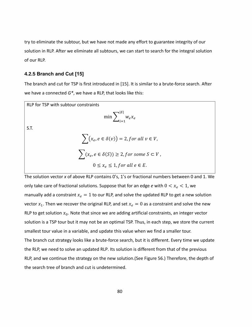
80

try to eliminate the subtour, but we have not made any effort to guarantee integrity of our

solution in RLP. After we eliminate all subtours, we can start to search for the integral solution

of our RLP.

4.2.5 Branch and Cut [15]

The branch and cut for TSP is first introduced in [15]. It is similar to a brute-force search. After

we have a connected G*, we have a RLP, that looks like this:

RLP for TSP with subtour constraints


|𝐸|

𝑖=1

S.T.

∑(𝑥𝑒 , 𝑒 ∈ 𝛿(𝑣)) = 2, 𝑓𝑜𝑟 𝑎𝑙𝑙 𝑣 ∈ 𝑉,

∑(𝑥𝑒, 𝑒 ∈ 𝛿(𝑆)) ≥ 2, 𝑓𝑜𝑟 𝑠𝑜𝑚𝑒 𝑆 ⊂ 𝑉 ,

0 ≤ 𝑥𝑒 ≤ 1, 𝑓𝑜𝑟 𝑎𝑙𝑙 𝑒 ∈ 𝐸.

The solution vector x of above RLP contains 0’s, 1’s or fractional numbers between 0 and 1. We

only take care of fractional solutions. Suppose that for an edge e with 0 < 𝑥𝑒 < 1, we

manually add a constraint 𝑥𝑒 = 1 to our RLP, and solve the updated RLP to get a new solution

vector 𝑥1. Then we recover the original RLP, and set 𝑥𝑒 = 0 as a constraint and solve the new

RLP to get solution 𝑥0. Note that since we are adding artificial constraints, an integer vector

solution is a TSP tour but it may not be an optimal TSP. Thus, in each step, we store the current

smallest tour value in a variable, and update this value when we find a smaller tour.

The branch cut strategy looks like a brute-force search, but it is different. Every time we update

the RLP, we need to solve an updated RLP. Its solution is different from that of the previous

RLP, and we continue the strategy on the new solution.(See Figure 56.) Therefore, the depth of

the search tree of branch and cut is undetermined.

81

Figure 56 Brach and cut

For each branch in Figure 56, it reaches the bottom if the solution vector is integral. If all

branches reach the bottom, the branch and cut searching terminates and we output the

bottom solution vector with smallest tour value; this solution corresponds to the optimal TSP

tour in G.

4.2.6 Some Thoughts on the Algorithm for TSP

A pseudocode of the process of the entire algorithm (from start of 4.2.1 to the end of 4.2.5) is

provided in Appendix C. The algorithm is implemented in the C programming language with

linear programming solver ILOG Cplex [21]. We try the program on a particular example with

100 vertices and 1012 edges; the running time of this example is 96.14 seconds which is not too

bad. This result is fantastic as compared to enumeration and dynamical programming. However,

there are still some remaining questions such as termination of the algorithm, the constrains in

RLP and why to choose this algorithm for connection graph.

Termination: As we claimed earlier, the termination of this algorithm is not guaranteed. This is

because we have no control on the depth of the searching tree of branch and cut. In fact, the

82

depth depends on the number of fractional coordinates of the solution vector in each RLP in the

searching tree, but we cannot know how many fractional solutions there are in a LP before

solving it. Therefore, it may happen that the number of fractional solutions increase or does not

change in one branch of the searching tree. In this case, the algorithm may not terminate in a

desirable time. A typical example of this phenomenon is running the algorithm on the pr76

problem (a problem instance from the TSPLIB [23]). The algorithm is unable to terminate after

two hours.

Constraints of the RLP: Even after adding all the subtour inequalities to an RLP, an integral

solution is not guaranteed. The reason is that a RLP with subtour inequalities is still not enough

to “describe” the TSP. (There is a quotation mark on the word describe, which means that it is

not an actual description by using words. In the next chapter, we will study the idea of this

“describe” in depth.) Simply speaking, we are still missing constraints; the missing constraints

are called comb inequalities [14]. Missing comb inequalities can cause a solution vector with

lots of fractional coordinates. It will also affect the depth of the search tree. Details about

comb inequalities are beyond the scope of this thesis.

Connection graph instance: One advantage of the connection graph is its sparseness. In our

applications, the number of edges in a connection graph is not very large. Therefore, the RLP of

connection graph does not have a lot of variables. This fact reduces the possibility of fractional

solution in RLP. In section 4.2.6, we see that the algorithm can solve a sparse graph with 100

vertices in a tolerable time, but it cannot solve the pr76 problem which is a dense graph with

76 vertices. We played a trick when we choose our algorithm for TSP: subtour elimination for

TSP is efficient in sparse graph, and connection graphs for our packed tubes problem are

sparse with no more than 100 vertices. We do not have an algorithm that is efficient in general,

but we do have an algorithm that is efficient in our case.


This chapter is the first chapter about the connection problem; it has two parts:

83

Part 1. Making a correspondence between the simplest one-path network system and a TSP

cycle in the connection graph.

Part 2. Solving the TSP in connection graph by subtour elimination [14] and branch cut

algorithm [15].

The first part converts the practical problem into a mathematical problem in graph theory. The

second part solves the mathematical problem using a known algorithm. Although we try to

design a simplest network system in a prism container, the mathematical representation of this

problem is one of the hardest problem in optimization. Fortunately, due to the particular

structure of connection graphs for packed tubes, TSP becomes solvable.

There are two points which still remain unanswered:

1. The weights of connection graphs. We still have not defined the weights in our

connection graph. As such we are solving TSP with arbitrary weights. There are

many choices for the weights. They can be distances between tubes, interference

ratios or types of connections between tubes. This is an open question for future

work.

2. The crossing edges. For example, in the connection graph of Figure 49, they are

edges crossing each other. They cannot be allowed in the same system. However,

our algorithm for TSP does not have this restriction.

In future, we will consider more complicated regions, i.e. containers with varying cross-

sections. In the situation, TSP will no longer correspond to a simple system because the

connection graph for each cross-section will be different.

84

Chapter 5 Connections in Varying Cross-sections

The one-path network is designed for the prism container, i.e. the packed tubes in each cross-

section have the same connection graph. In reality, the container could have different cross-

sections. For example, the tubular network system in Figure 41 (Section 3.2), it is designed for a

dumbbell shape container. The packing of tubes in first two cross-sections is shown on Figure

57. There are 9 circles in the first cross-section which is enclosed by the black square. There are

4 circles in the second cross-section which is enclosed by the red dashed line square region in

the bottom left corner.

Figure 57 simple example on

changing cross-sections

Figure 58 The example in all 4 sections

Note that Figure 57 illustrates the cross-sections and packed tubes only at the first two

transition parts of the system in Figure 41 --- the packing at one end and the packing on both

sides of the transition from the outer “bag” to the inner region. The third cross-section has 4

circles and the fourth cross-section has 9 circles. They are symmetric to cross-sections 1 and 2,

respectively. As shown in Figure 58, the red part is the third cross-section, which is identical to

the red dashed line square in Figure 57.

Since the connection graphs in different cross-section may be different, it is obvious that one

mathematical instance for designing such a complicated system will not be adequate. In order

to start, we will find a mathematical instance in graph theory corresponding to connections in

one cross-section, i.e. we only connect tubes in one cross-section despite the fact that we are

85

connecting network involving all cross-sections of the container. Therefore, our algorithm for

connection works in one connection graph. This is basically the first step of connection in

multiple cross-sections. Finding a connection for multiple cross-sections still remains an open

problem for the future work. But before finding our algorithm, the most important thing is to

understand how tubes change when the cross-sections change, i.e. what happens in the two

big cubes in Figure 58. Thus, the first part of this chapter is about operations between tubes.

5.1 Operations between Tubes [24]

Recall our rules for fundamental elements as stated in section 3.1, all operations between tubes

should be decomposable into combinations of finite elements. An end-cap is one operation

formed by two L-blocks or modified L-blocks. It does not change the number or position of

tubes. The operations described in this section are used in networks with varying cross-sections.

As such, they will be used to change the number or position of tubes [24]. All of these

operations are formed by fundamental elements.

1. Merge operations.

Figure 59 Single merge and its decomposition

Figure 60 Consecutive merge

Merge operations will merge two tubes into one tube. A simplest merge operation is the single

merge shown in Figure 59: Tube 1 and tube 2 merge into one tube at tube 2’s position. From

Figure 59, it is easy to see that a single merge can be decomposed into three I-block, a T-block

and a L-block or modified L-block. If the sizes of tube 1 and tube 2 are different, we shall use

modified L-block. Otherwise, we use an unmodified L-block.

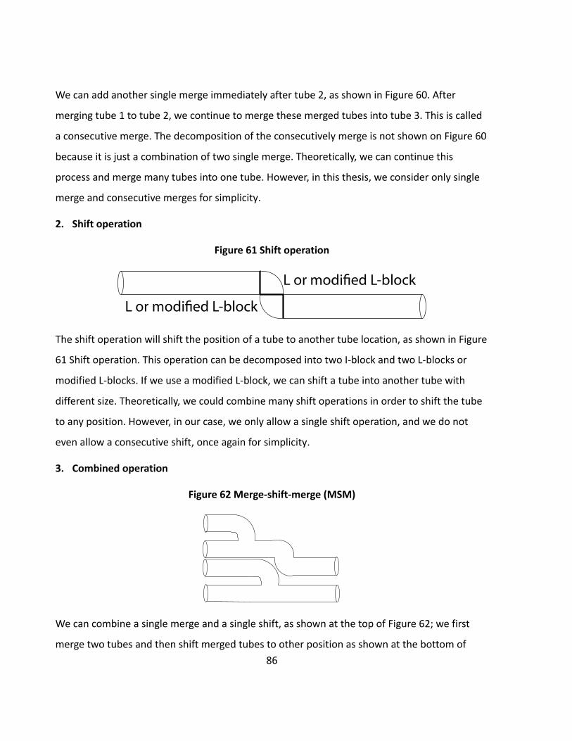
86

We can add another single merge immediately after tube 2, as shown in Figure 60. After

merging tube 1 to tube 2, we continue to merge these merged tubes into tube 3. This is called

a consecutive merge. The decomposition of the consecutively merge is not shown on Figure 60

because it is just a combination of two single merge. Theoretically, we can continue this

process and merge many tubes into one tube. However, in this thesis, we consider only single

merge and consecutive merges for simplicity.

2. Shift operation

Figure 61 Shift operation

The shift operation will shift the position of a tube to another tube location, as shown in Figure

61 Shift operation. This operation can be decomposed into two I-block and two L-blocks or

modified L-blocks. If we use a modified L-block, we can shift a tube into another tube with

different size. Theoretically, we could combine many shift operations in order to shift the tube

to any position. However, in our case, we only allow a single shift operation, and we do not

even allow a consecutive shift, once again for simplicity.

3. Combined operation

Figure 62 Merge-shift-merge (MSM)

We can combine a single merge and a single shift, as shown at the top of Figure 62; we first

merge two tubes and then shift merged tubes to other position as shown at the bottom of

87

Figure 62. After combining a single merge and a single shift, we can put another single merge

in the space made available by the shift. This operation is called merge-shift merge; it changes

the number of tubes from 4 to 2. We shall consider only this combined operation in this thesis.

In summary, the only operations we considered in this thesis are single merge, consecutive

merge, single shift and merge shift merge.

Note that for the purpose of good visualization aspect, in our figures of operations, our figures

of operations will show the tubes to be in the same plane. In reality, we can rotate the tubes in

the operations with respect to some axis.

5.1.1 Connection between Operations

We now apply the operations described in preceding the to the network in Figure 57; 9 tubes

in first cross-section will become 4 tubes in next cross-section. Here is an example of how to

use operations to perform this change of cross-sections:

Figure 63 An example of application of operations

In Figure 63, the red lines denote operations. The red line with a length of two times of circle

radii represents the single merge operation; from the figure we see that tube 7 merges to tube

4. The red line with length of four circle radii represents the consecutive merge operation; tube

9 merge to tube 8 and together they merge to tube 5. The red line with length of six circle radii

represents the merge-shift-merge operation; tube 6 merges to tube 3 and together they shift

88

to tube 2’s position, and then tube 2 merges to tube 1. The arrows in the figure show the

direction in which they operate.

Figure 63 displays only one possible combination of operations. There are many combinations

of operations to reach the same goal. For more examples, please see [24].

Now we suppose we have already had a combination of operations and we want to connect

tubes in different operations by end-caps. If we connect two tubes in one cross-section, we

need to find a set of end-cap connections such that each end-cap connection is disjoint from

the others. This is equivalent to finding a set of disjoint edges in connection graph. In addition,

we need to modify our connection graph in order to form a feasible network [24]:

The edge formed by tubes in a single merge operation should be deleted.

The edge formed by tubes in the first two positions of a consecutive merge

operation should be deleted.

If an inlet or outlet is in any operation, we delete the corresponding vertex from

connection graph.

With such modified connection graph, we can treat our connection in one cross-section

problem as a matching problem in this graph.

5.2 Cutting Plane for Matching [26]

Definition 10 Matching. [27] In a graph G= (V, E), a matching M is a subset of E for which no

edges in M share the same end-point. A vertex is in a matching M if it is an end-point of

an edge in M. In this case, we say that this vertex is matched by M.

From the definition, a matching is exactly a set of edges such that each edge is disjoint from

others. However, a feasible matching may not correspond to a feasible connection in a cross-

section. In fact, a feasible connection should connect all tubes in the cross-section. Therefore,

we want a matching that matches all vertices in the modified connection graph. In graph

theory, a matching that matches all vertices is called a perfect matching, denoted as PM. Note

89

that a PM may not exist, here we assume that PM exists as we will focus on solving it. We

assign each edge an arbitrary weight 𝑤𝑒, and wish to find the PM for which the total weight of

edges in it is maximized or minimized. This is called an optimal PM.

Optimal PM is also a well-studied problem in combinatorial optimization. Unlike TSP, optimal

PM can be solved in polynomial time. The most famous algorithm is the Blossom algorithm

invented by Edmonds in 1965 [31]. It is a polynomial time algorithm with complexity 𝑂(|𝑉|4),

and there is an efficient C++ implementation of this algorithm [33]. Due to the difficulty of

implementation of the Blossom algorithm, we shall solve PM in another method. Recalling the

idea of the cutting plane, we will use cutting plane method to solve PM [26]. Fortunately, the

termination of cutting plane method for PM is guaranteed. Therefore, no branch and cut

search is required.

5.2.1 A General View of the Cutting Plane Method for Perfect Matching (PM)

In a manner similar to that described in 4.2.1. We could define the characteristic vector of a

PM as

𝑥𝑒 = {1, 𝑖𝑓 𝑒 𝑖𝑛 𝑐ℎ𝑜𝑠𝑒𝑛 𝑖𝑛 𝑜𝑝𝑡𝑖𝑚𝑎𝑙 𝑃𝑀,0, 𝑜𝑡ℎ𝑒𝑟𝑤𝑖𝑠𝑒.

The IP for PM is

IP for perfect matching


|𝐸|

𝑖=1

s.t.

∑(𝑥𝑒 , 𝑒 ∈ 𝛿(𝑣)) = 1, 𝑓𝑜𝑟 𝑎𝑙𝑙 𝑣 ∈ 𝑉 ,

𝑥𝑒 = {0,1}, 𝑓𝑜𝑟 𝑎𝑙𝑙 𝑒 ∈ 𝐸.

The constraint ∑(𝑥𝑒 , 𝑒 ∈ 𝛿(𝑣)) = 1, 𝑓𝑜𝑟 𝑎𝑙𝑙 𝑣 ∈ 𝑉 means that each vertex is matched only

once by the PM. Since every vertex is matched, these equalities must hold.

90

As was the case for the IP for TSP, we relax the IP for PM by setting 0 ≤ 𝑥𝑒 ≤ 1. However, due

to the constraints on vertices, we only need that 𝑥𝑒 ≥ 0. The result is a relaxed linear

programming for the IP of PM.

However, solving this RLP does not give a matching, i.e. there may be fractional solutions in the

solution vector. A example of such a fractional solution of RLP is shown in Figure 64. From the

figure, it can be seen that the problem of fractional solutions is caused by subset with odd

number of verteices.

Figure 64 Example of fractional solution in odd set

For each odd subset of vertex 𝑺 ⊆ 𝑽, a feasible matching can only match at most |𝑺| − 𝟏 vertices,

which means that at most |𝑺|−𝟏

𝟐 edges can be matched. An integral solution of RLP automatically

implies this, but a fractional solution does not. Let 𝜸(𝑺) (not the interference ratio) denote the set

of edges uv such that 𝒖 ∈ 𝑺 𝒂𝒏𝒅 𝒗 ∈ 𝑺. We can write above argument in terms of an inequality:

∑(𝑥𝑒 , 𝑒 ∈ 𝛾(𝑆)) ≤|𝑆| − 1

2, ∀𝑆 ⊂ 𝑉, |𝑆| = 𝑜𝑑𝑑

This inequality is called the blossom inequality [31]. It must hold for a solution of feasible

matching. Since S is any odd subset of V, there are 2|𝑉|−1 such inequalities. As our argument in

last chapter, we do not need to add them all. We only need to find the subsets S for which the

blossom inequalities are violated by S. We then add the blossom inequalities for S to our RLP.

This strategy is exactly same as was used by the cutting plane method in TSP. However, by

adding blossom inequalities, the termination of cutting plane method for PM is guaranteed. In

TSP, adding all subtour inequalities cannot guarantee termination. The reason for this

91

difference will be explained in subsection 5.2.4. A flow chart of the entire algorithm is

described below:

Algorithm 8 Cutting Plane Method for Perfect Matching [26]

∎

There are a number of unclear points in this flow chart that will be explained in the next two

subsections.

92

5.2.2 Step 1-Step 4 and Step 6-7: General Process of Cutting Plane Method

Step 1~3, 6 and 7 are exactly same as in the cutting plane method for TSP. We just solve the

RLP and determine if the solution vector is integral. Step 6 is just adding cutting planes to the

RLP and solve the new RLP again. Step 7 is a criterion that an integral solution corresponds to

the optimal solution in original IP.

Step 4 is a little different from the cutting plane method for TSP: We construct G* by adding

these edges in G with non-zero RLP solutions, but G* has a weight on each edge with 𝑤𝑒∗ =

𝑥𝑒∗ if 𝑒∗ is an edge in both G and G*. In some books, this step is referred to as “blossom

inequalities for some cuts”. Blossom inequalities, however, are defined for 𝛾(𝑆) instead of

cuts. Recall Definition 7 about 𝛿(𝑆) (the cut of vertex subset S). This definition is totally

opposite to 𝛾(𝑆) in the blossom inequality. That being said, the arguments of the two

definitions are actually not in conflict. In fact, the blossom inequality has two forms:

∀𝑆 ⊂ 𝑉, |𝑆| = 𝑜𝑑𝑑

∑(𝑥𝑒 , 𝑒 ∈ 𝛾(𝑆)) ≤|𝑆| − 1

2⟺ ∑(𝑥𝑒 , 𝑒 ∈ 𝛿(𝑆)) ≥ 1

The LHS is the original blossom inequality and the RHS is called blossom inequality of cut form.

They two are equivalent. For details about the proof, please see Appendix D.

Since there is a ready-made algorithm to find cuts with a specific value, using the blossom

inequality for cut as cutting plane is more convenient. In fact, the purpose of step 5 is to find a

cut in G*=(𝑉, 𝐸∗, 𝑥𝑒∗) with total weight less than 1.

5.2.3 Step 5: Odd Cuts in G*

In step 5, the Padberg and Rao procedure [30] uses Gomory-Hu tree [26] to find an odd cut

with weight less than 1. In order to understand the procedure, we need to understand the

Gomory-Hu tree of G* (in short GH(G*)).

Definition 11 Tree. A tree is a connected graph with no cycle.

93

Definition 12 Gomory-Hu Tree. [28] The Gomory-Hu tree of graph G*=(𝑉, 𝐸∗, 𝑥𝑒∗) is defined

by

𝑉(𝐺𝐻(𝐺∗)) = 𝑉(𝐺∗), ∀𝑢, 𝑣 ∈ 𝑉(𝐺∗), 𝑖𝑓 𝑢𝑣 ∈ 𝐺𝐻(𝐺∗), 𝑡ℎ𝑒𝑛 𝑤𝑢𝑣 = 𝑀𝐴𝑋𝐹𝐿𝑂𝑊(𝑢, 𝑣, 𝐺∗);

𝑖𝑓 𝑢𝑣 ∉ 𝐺𝐻(𝐺∗), 𝑡ℎ𝑒𝑛 min{𝑤𝑖𝑗: 𝑖𝑗 ∈ 𝑃𝐴𝑇𝐻(𝑢, 𝑣, 𝐺𝐻(𝐺∗))} = 𝑀𝐴𝑋𝐹𝐿𝑂𝑊(𝑢, 𝑣, 𝐺∗);

𝑙𝑒𝑡 𝑚𝑛 = {𝑚𝑛 ∈ 𝐺𝐻(𝐺∗): 𝑤𝑚𝑛 = 𝑚𝑖𝑛{𝑤𝑖𝑗: 𝑖𝑗 ∈ 𝑃𝐴𝑇𝐻(𝑢, 𝑣, 𝐺𝐻(𝐺∗))} ,

𝑡ℎ𝑒𝑛 𝑟𝑒𝑚𝑜𝑣𝑒 𝑒𝑑𝑔𝑒 𝑚𝑛 𝑖𝑛 𝐺𝐻(𝐺∗)𝑔𝑖𝑣𝑒𝑠 𝑡𝑤𝑜 𝑐𝑜𝑚𝑝𝑜𝑛𝑒𝑛𝑡𝑠 𝑎𝑛𝑑 𝑡ℎ𝑒 𝑐𝑜𝑚𝑝𝑜𝑛𝑒𝑛𝑡𝑠 𝑔𝑖𝑣𝑒𝑠 𝑎

𝑚𝑖𝑛𝑚𝑢𝑚 𝑐𝑎𝑝𝑎𝑐𝑖𝑡𝑦 𝑢 − 𝑣 𝑐𝑢𝑡 𝑖𝑛 𝐺∗

In this definition, 𝑀𝐴𝑋𝐹𝐿𝑂𝑊(𝑢, 𝑣, 𝐺∗) corresponds to the maximum flow between node v and

u in graph G*. 𝑃𝐴𝑇𝐻(𝑢, 𝑣, 𝐺𝐻(𝐺∗)) denotes the path between u and v in Gomory-Hu tree of

graph G*.

We can compute the GH tree by a very simple algorithm [28]. This algorithm first computes

maximum flow between all pairs of vertices, and then use the vertices of G* and flow values to

construct a tree. The maximum flow between two vertices can be computed by the Ford-

Fulkerson algorithm [29] in 𝑂(𝑉𝐸∗2) time. This simple algorithm uses |V|(|V| − 1) times

computation of maximum flow. Therefore, obtaining GH(G*) by this algorithm has a complexity

𝑂(𝑉3𝐸∗2).

Once we have a GH tree of G*, we can search for edges in GH(G*) with edge weights less than

one. This can be done by a depth-first search which has a complexity O(V). If we find an edge in

GH(G*) with weight less than 1, we delete this edge. The two components yielded by deleting

this edge will be a cut in G* with cut weight less than 1. If the component size is odd, this cut is

exactly the cut which violates the blossom inequality for cut. We add the blossom inequality of

the smaller component to RLP, and we retrieve the deleted edge in GH(G*). If the component

size is even, we continue to search other edges. We respect above procedure until we have

investigated all edges in GH(G*) with edge weights less than one. This method is called the

Padberg and Rao procedure [30].

The Padberg and Rao procedure guarantees to produce odd cuts that violate the blossom

inequality [26]. The drawback of the Padberg and Rao procedure is its price. Since depth-search

94

only takes 𝑂(𝑉), the most consuming part of Padberg and Rao is computing GH(G*). The

complexity of Padberg and Rao procedure is 𝑂(𝑉3𝐸∗2 + 𝑉) = 𝑂(𝑉3𝐸∗2).

After we add the blossom inequalities of all odd cuts produced by Padberg and Rao to the RLP,

we solve the RLP again and go through step 3-6 until we have an integral solution vector.

However, how do we know that Algorithm 8 will terminate with an integral vector? We do not

have any techniques like branch and cut to keep solution integral. In fact, the answer to this

question is given in the statement at the end of section 5.2.1; we need to understand the

difference between TSP cutting plane and PM cutting plane.

5.2.4 Termination of Algorithm 8

We need to understand the characteristic vectors of matching in high dimensional space.

Definition 13 Convex Hull. [27] The convex hull of a finite set S is the set of all vectors that

can be written as a convex combination of elements S.

As an example in 2.4.5, a line segment is the convex hull of its two end-points.

Definition 14 Perfect Matching Polytope. [27] The convex hull of characteristic vectors of all

perfect matchings are called the perfect matching polytope.

From the above definition, we could see that the perfect matching polytope is a polyhedral in

high dimensional space.

The RLP for PM with blossom inequalities are


|𝐸|

𝑖=1

s.t.

∑(𝑥𝑒 , 𝑒 ∈ 𝛿(𝑣)) = 1, 𝑓𝑜𝑟 𝑎𝑙𝑙 𝑣 ∈ 𝑉 ,

∑(𝑥𝑒 , 𝑒 ∈ 𝛿(𝑆)) ≥ 1, ∀𝑆 ⊂ 𝑉, |𝑆| = 𝑜𝑑𝑑,

𝑥𝑒 ≥ 0.

95

In [27],a theorem called Matching Polytope Theorem is proved. One corollary of the theorem

states that the perfect matching polytope is defined by the above RLP. Moreover, the blossom

inequalities are exactly the hyperplanes of the perfect matching polytope. Therefore, adding

blossom inequalities is equivalent to adding hyperplanes. If we solve our RLP, the solution will

be one of the extreme points of the perfect matching polytope. Keeping on solving RLP will

keep on searching on the extreme points of perfect matching polytope, and by Definition 14,

the extreme points will contain characteristic vectors of perfect matchings; therefore, we can

definitely terminate at a integral solution which is a perfect matching that minimizes the

objective function. As a result, an integral solution is guaranteed by solving the RLP with added

blossom inequalities.

On the contrary, an RLP with subtour inequalities does not define the TSP polytope (The convex

hull of all TSP characteristic vector.) Therefore, solving RLP with subtour elimination will not

search the extreme points of the TSP polytope. The algorithm may not necessary terminate at

an integral solution which corresponds to a TSP tour.

5.2.5 Running Time of Algorithm 8

Algorithm 8 is implemented in C++ with ILOG Cplex Optimization Library. We run the program

on 1000 random graphs with 1000 vertices. Figure 65 are the histogram and scatter plot of

running time of 1000 random graph.

From the results in Figure 65, we could see that cutting plane for matching is not slow. In most

graphs with 1000 vertices it can find an optimal matching within 25 seconds. There is only one

outlier in our 1000 random graphs which takes more than 1500 seconds. On the other hand,

finding a TSP in a sparse graph with 100 vertices can take 90 seconds. Therefore, the matching

problem is much easier than TSP, but we cannot use matching to solve TSP.

96

Figure 65 Running time results

5.3 Bifurcation End-cap and b-matching

Now we consider a more general end-cap: An end-cap with two tubes merging into one tube.

Since it can be decomposed into fundamental elements (as shown on Figure 66), it is a

theoretically feasible connection. We shall refer to this end-cap as a bifurcation end-cap.

Figure 66 Bifurcation end-cap

The bifurcation end-cap is constructed with a T-block and two L or modified L-block. Since we

allow modified L-blocks, merging tubes with different radii is also allowed.

97

The only issue of bifurcation end-cap is the “T-block”. This “T-block” will be different from

what was discussed in 3.1. A sketch of this “T-block” is presented in Figure 67. We can see that

this “T-block” has an angle at the bottom tube of the T-block. Its geometry is an open problem

and it is beyond the scope of this thesis. For the remaining of this thesis, we treat the “T-

block” in bifurcation end-cap as the T-block in 3.1.

Figure 67 “T-block” in bifurcation end-cap

Based on the above discussion, the bifurcation end-cap is not qualified to be a feasible

operation for tube connection. However, from this operation one can derive a series of

interesting matching problem. By Definition 10, a matching can match a vertex only once, i.e. a

tube can connect to another tube only by means of an end-cap. However, we can now also

connect two tubes to one tube with a bifurcation end-cap. This is equivalent to allow a

matching which connects some vertices twice. In combinatorial optimization, there is a

general instance which describes this type of matching.

Definition 15 b-matching [27]. Suppose a vector 𝑏 ∈ 𝑍|𝑉|, for each vertex v, a matching 𝑀 ⊂

𝐸 with |𝑀 ∩ 𝛿(𝑣)| = 𝑏𝑣 is called a b-matching.

From the definition of b-matching, if 𝑏 = 𝟏|𝑉|, the b-matching is simply a perfect matching. In

our case, we want 𝑏 = {1,2}|𝑉|, i.e. for some tubes, we want them to be connected with two

other tubes; for other tubes, we want them to be connected with only one other tube.

98

5.3.1 Solving b-matching

Sometimes b-matching is called as “general matching”. The first algorithm for b-matching is

given by Pulleybank in his Phd thesis [25]. The algorithm borrows the idea of blossom

algorithm and generalizes it to general matching. It is not polynomial time algorithm, however,

since our b value is not large (less than 3), we can solve our b-matching problem using

Algorithm 8 Cutting Plane Method for Perfect Matching. We modify our graph G to a produce

new graph Gb, and apply Algorithm 8 on Gb to get a optimal perfect matching in Gb. The

optimal PM in Gb corresponds to the optimal b-matching in G. This procedure, as shown in

Figure 68, is called data reduction and it is invented by Tutte in 1957 [27].

Figure 68 Data reduction for b-matching

∎

Although this process is polynomial time, it will increase the problem size of the perfect

matching. Since 𝑏 = {1,2}|𝑉|, Gb will have a vertex set that is almost twice of G and an edge

set that is almost four times of G. Fortunately, our b vector is not too large; Gb is not largely

increased in size. Moreover, if the L-1 norm of b is bounded by a polynomial function of the

problem instance, solving b-matching by combining Algorithm 8 and data reduction for b-

matching is strong polynomial time [27]. Since we only allow T-block, L-block, modified L-block

99

and I-block, we cannot form an end-cap that connects more than two tubes to one tube.

Therefore, L-1 norm of b in the connection graph is no larger than 2, and finding a b-matching

in connection graph is polynomial time [27].

Therefore, we can conclude that finding a connection with bifurcation end-cap is as hard as

finding a connection with end-cap only if we use matching instance to find connection.


The situation treated in this chapter is more complicated than Chapter 4. Here we have

multiple cross-sections, and each of them has its own circle packing; there are also operation

between tubes in a cross-section. In this case, we cannot associate a feasible network with a

single mathematical instance like TSP. Thus, instead of finding a feasible network for the whole

system, we try to connect tubes in each cross-section individually. Note that assembling

optimal connections in each cross-section may not provide an optimal network system, but an

optimal connection in one cross-section is a good reference for designing the whole system.

Therefore, it is beneficial to study the optimal connection in one cross-section.

We reduce the connection in one cross-section into a matching problem in the connection

graph of the given cross-section. The general matching problem is a classical problem in

combinatorial optimization, and it is a problem can be solved with a polynomial time

algorithm. Since our connection graph is sparse, we can apply the cutting plane method to

matching for the same reason as TSP. Unlike TSP, Algorithm 8 Cutting Plane Method for Perfect

Matching is guaranteed to terminate because of the structure of the matching polytope.

Furthermore, we generalize our connection in one cross-section to allow two tubes connect to

one tube. This generalization requires a more general version of matching called b-matching.

The b-matching can be solved by solving perfect matching and data reduction. Since our

connection graph is always sparse, solving b-matching in the connection graph is polynomial.

Therefore, we conclude that b-matching is as hard as perfect matching in connection graph.

100

In conclusion, the matching algorithm (including the b-matching) does not provide an optimal

network for the system. Combining optimal connections in each cross-section can not yield an

optimal system. For example, in Chapter 4, we could not solve TSP by solving perfect matching

on both ends individually, so optimal connections on each end do not yield an optimal one-

path system. However, optimal matching on each cross-section provides a good reference for

examining the quality of whole network system.

101

Chapter 6 Conclusion and Future Works

In this thesis, we have divided our problem of designing tubular networks system in an

arbitrary container exhibiting longitudinal symmetry into two parts:

1. Packing tube cross-sections into the container cross-sections. We reduce this problem to

a circle packing problem.

2. Connecting packed tubes in the blocks to produce a system. For the prism container, we

solve this by solving TSP. For varying cross-sections, we try to solve for each cross-section

independently by using matching; but the optimal connection in each cross-section does

not give an optimal network system.

Tube connections are based on packed tubes. We have defined fundamental elements,

interference ratio and connection graph in order to translate the information of packed tubes to

the instance for connection.

6.1 Conclusions

Now we will conclude the two parts mentioned above.

6.1.1 Part 1: Circle Packing

In the circle packing chapter, we have investigated two major circle packing algorithms:

1. GGL algorithm.[2] This algorithm places circles in a rectangle along three positions:

corners, a side and an existing circle and two existing circles. For each existing circle, a

position number is defined as the number of all possible positions to place a new circle

along the circle. The GGL algorithm places a new circle based on the position number of an

existing circle. Since the GGL algorithm uses the shape of region as packing reference, the

packing density of the result is good (around 70%-80%, see 2.2.5). The complexity of GGL is

polynomial, and it is at least 𝑂(𝑁3). This means the algorithm is not efficient, but it is

102

enough for our design purpose since there will be no more than one hundred tubes in one

cross-section.

We also generalize the GGL algorithm to more complicated regions such as trapezoid or L-

shaped regions. This generalization dos not modify the idea of GGL; it only requires

changing the number of feasible positions for each circle since there are unparalleled sides

in trapezoid and more sides and corners in L-shaped region. Therefore, the complexity of

GGL in complicated region is same as GGL in rectangle.

As a conclusion, working on GGL algorithm is on the right track since its idea can be

generalized to more complicated regions without a great deal of modification. However,

due to flow and heat transfer issues [5], we want to place big circles in the center of the

cross-section, but GGL will always try to place large circles at corner or along sides.

Therefore, anti-GGL is developed based on the concept of position number in GGL, but it

approaches in an exactly opposite direction.

2. Anti-GGL Algorithm.[6] In anti-GGL, we start with placing a large circle in the centroid of

the region, and we put a circle next to the first circle immediately. Then place new circles

along two existing circle. Note that in anti-GGL, we do not use corner or sides as reference

to place new circles, so the position number in anti-GGL is much simpler than GGL.

According to this fact, we generalize anti-GGL algorithm to an arbitrary polygon. The

packing density of anti-GGL is not as good as GGL, but it can be improved by jiggling [24].

Moreover, we also develop an algorithm to shrink the polygonal region by a certain

distance; this algorithm is helpful when we want to keep tubes away from the boundary of

container.

In practical, we use anti-GGL with shrinking as the algorithm for packing tubes.

6.1.2 Part 2 Connection between Tubes

1. Foundations for Connection. The foundations for connection are fundamental elements,

interference ratio and connection graph. The fundamental elements are I-block, L-block, T-

103

block and modified L-block; every operation and connection can be decomposed to

combination of finite fundamental elements, i.e. the end-cap connection can be

decomposed to two L-blocks. The interference problem occurs when the end-cap

connection for connecting two tubes overlaps with a third tube. An “interference ratio” is

defined to characterize quantitatively the interference between two tubes. This ratio is

used as a criterion to determine if two tubes are eligible to be connected by end-cap. We

store all pairs of tubes that are eligible to be connected in a connection graph. Each edge in

connection graph corresponds to an end-cap connection of the endpoints. As a result, we

translate the circle packing result to a connection graph in which we will make connection

decisions.

2. One-path Network. If we connect every tube to form one long tube, this network system

is called one-path network. This network only exists in packed tubes of a prism container, i.e.

the redneck barbeque pool heater. Since the connection graphs at all cross-sections are the

same, we can correspond the one-path network system to a travelling salesman problem

(TSP) in the connection graph. The TSP is NP-hard, but we can solve it for small graphs. As we

have no more than one hundred tubes in any one cross-section and the connection graphs

are sparse, we can apply the idea of the cutting plane for solving TSP [14]. However, TSP

cannot be solved with only cutting planes; we also need to branch and cut search [15] based

on the result of cutting plane. Since the search tree of branch and cut is undetermined, this is

a non-deterministic algorithm for which termination is not guaranteed. It does work,

however, in our connection graphs.

3. Connections in Varying Cross-sections. If the cross-sections are varying, we are unable

to construct one-path networks. In this case, we define operations that connect the tubes

between two different cross-sections; then we connect these operations by end-cap.

Instead of forming a complete network system, we connect tubes at each cross-section

independently. We reduce this problem to a perfect matching problem on connection

graph of each cross-section. The perfect matching problem can also be solved via the

104

cutting plane method. In fact, due to the structure of matching polytope [27], cutting plane

algorithm for perfect matching [26] is a deterministic algorithm and no branch and cut

search is required. Our result shows that cutting plane for matching is efficient in a graph

with 1000 vertices. However, assembling perfect matching on each cross-section may not

provide a feasible network system. Therefore, designing a complete tubular network

system in varying cross-sections still remains an open problem, but perfect matching on

each cross-section could be an important reference for future work.

6.1.3 Emphasizing the Difference between This Thesis and [24]

In Wenzhe Jiang’s MMath thesis [24], the author uses depth-first search and minimum degree

matching to find all feasible solutions for connection problem associated with a given tubular network.

A "best solution" may then be found by examining every feasible solution. In this thesis, however, we

have tried a different approach. We convert the connection problem into a TSP or perfect matching

problems in the corresponding connection graph. By solving these optimal TSP and PM problems, the

solutions may correspond to an optimal connection design in the tubular system. This method does not

enumerate every possible connection; it will produce one optimal solution. The only one exception is in

the case of the branch and cut method for TSP. In fact, the solutions to the RLPs at the bottom of the

tree in Figure 56 are all integer valued. Therefore, the solutions to these RLPs correspond to TSP tours

in a connection graph, but they may not to be optimal TSP tours. Since we know that each TSP tour in

connection graph corresponds to a one-path network, we have produced more than one feasible

solution for the connection problem. However, we do not try to generate all feasible solutions.

6.2 Future Works

Here are some open problems:

6.2.1 Non-simple Connected Cross-section

In this thesis, all cross-sectional regions have been assumed to be simple connected, i.e. there

is no holes. Here is an example of a non-simply connected region:

105

Figure 69 Non-simple connected region

Packing circles in region D is a future direction. In Figure 69, the center of circle should be in

polygon D but not in P. By applying Algorithm 2 Crossing number algorithm , this constraint is

not hard to implement.

6.2.2 Weights on Connection Graph

In section 4.1.3 and 5.1.1, in these chapters, we mentioned that the weights 𝑤𝑒 are not

specified in connection graph. We considered 𝑤𝑒 as arbitrary positive numbers and solve TSP

and matching in general instance. In fact, as a design problem, 𝑤𝑒 should have some physical

meaning. A common example of representation of 𝑤𝑒 is the Euclid distance between the

centers of two tubes, but 𝑤𝑒 can be more meaningful. For example, 𝑤𝑒 can represent flow

resistance factor or heat transfer between tubes or interference between two tubes.

6.2.3 Connection Graph of System

In section 3.3 Graph Representation for Possible Connection, the connection graph is

constructed for one cross-section, and this assumption holds through the whole design

process. In fact, problems arise in Chapter 5 when connecting tubes in varying cross-section.

Since connection graphs are different in different cross-sections, we have to connect each

cross-section independently. A possible way to resolve this problem is to construct connection

graph for the whole network system. For example, the 9-4-9 problem in Figure 58:

106

Figure 70 Incomplete network system for 9-4-9

Figure 70 is an example of incomplete network system with only operations, the numbers are

tubes. Constructing a connection graph based on this system is essential in order to find a

feasible network system.

6.2.4 CAD Work for Tubular Network System

In this thesis, our discussion has focused more on formulating design problem as mathematical

instance such as circle packing, TSP and matching. We have actually provided very few visual

examples. However, a computer 3D model would be very beneficial to comprehending our

design purpose. Here is a visual example of what we want to design: Figure 71 is a SolidWork

3D model of a 9-4-9 system.

Figure 71 3D model for 9-4-9

107

The system in Figure 71 is not designed by any of the methods developed in this thesis. The

packing and connection were this example are done by hand [24]. In future, we make

correspondence between the abstract mathematical results to computer 3D model like Figure

71. This will be the most practical work among all future works.

108

Appendix A

Derivation the parameterization of modified L-block

Recall the parameterization of a torus:

𝑥(𝜃, 𝜑) = (𝑅 + 𝑟𝑐𝑜𝑠𝜃)𝑐𝑜𝑠𝜑,

𝑦(𝜃, 𝜑) = (𝑅 + 𝑟𝑐𝑜𝑠𝜃)𝑠𝑖𝑛𝜑,

𝑧(𝜃, 𝜑) = 𝑟𝑠𝑖𝑛𝜑 ,

𝜃 𝑎𝑛𝑑 𝜑 𝑎𝑟𝑒 𝑎𝑛𝑔𝑙𝑒𝑠 𝑤ℎ𝑖𝑐ℎ 𝑚𝑎𝑘𝑒 𝑎 𝑓𝑢𝑙𝑙 𝑐𝑖𝑟𝑐𝑙𝑒, 𝑖. 𝑒. 0 ≤ 𝜃, 𝜑 ≤ 2𝜋,

𝑅 𝑖𝑠 𝑡ℎ𝑒 𝑑𝑖𝑠𝑡𝑎𝑛𝑐𝑒 𝑓𝑟𝑜𝑚 𝑡ℎ𝑒 𝑐𝑒𝑛𝑡𝑒𝑟 𝑜𝑓 𝑡ℎ𝑒 𝑡𝑜𝑟𝑢𝑠 𝑡𝑜 𝑡ℎ𝑒 𝑐𝑒𝑛𝑡𝑒𝑟 𝑜𝑓 𝑡ℎ𝑒 𝑐𝑖𝑟𝑐𝑢𝑙𝑎𝑟 𝑡𝑢𝑏𝑒 𝑜𝑓 𝑟𝑎𝑑𝑖𝑢𝑠 𝑟.

From above figure of the modified L-block. We could see that it can be generated in a way

quite similar to torus, with the following exceptions:

1. The inner radius is zero.

2. The tube radius is a function with respect to 𝜑

3. The center line of modified L-block is an ellipise with semi-major axis R1 and semi-minor

axis R2.

Now, based on above three characteristics of modified L-block, we can construct its

parameterization as follows.

First, since the inner radius is zero, so that 𝑟 = 𝑅

109

𝑥(𝜃, 𝜑) = (𝑅 + 𝑅𝑐𝑜𝑠𝜃)𝑐𝑜𝑠𝜑,

𝑦(𝜃, 𝜑) = (𝑅 + 𝑅𝑐𝑜𝑠𝜃)𝑠𝑖𝑛𝜑,

𝑧(𝜃, 𝜑) = 𝑅𝑠𝑖𝑛𝜑.

Note that 𝑅 = 𝑅(𝜑). Since the center of the tube exhibits an elliptical path, we can employ the

the equation of an ellipse in polar coordinates:

𝑅(𝜑) =𝑅1𝑅2

√(𝑅1 cos(𝜑))2 + (𝑅2 sin(𝜑))2,

𝑤ℎ𝑒𝑟𝑒 𝑅1, 𝑅2 𝑎𝑟𝑒 𝑚𝑖𝑛𝑜𝑟 𝑎𝑛𝑑 𝑚𝑎𝑗𝑜𝑟 𝑎𝑥𝑒𝑠 𝑟𝑒𝑠𝑝𝑒𝑐𝑡𝑖𝑣𝑒𝑙𝑦.

Then, we substitute 𝑅(𝜑) to obtain

x(θ, 𝜑) =𝑅1𝑅2(1 + 𝑐𝑜𝑠𝜃)𝑐𝑜𝑠𝜑

√𝑅12 cos2 𝜑 + 𝑅22 sin2 𝜑,

y(θ, 𝜑) =𝑅1𝑅2(1 + 𝑐𝑜𝑠𝜃)𝑠𝑖𝑛𝜑

√𝑅12 cos2 𝜑 + 𝑅22 sin2 𝜑,

z(θ, 𝜑) =𝑅1𝑅2𝑠𝑖𝑛𝜃

√𝑅12 cos2 𝜑 + 𝑅22 sin2 𝜑.

The above result is the parameterization of modified L-block as required.

110

Appendix B

Improvement of Algorithm 7

When we pack circles using either GGL or anti-GGL algorithms, we need to check the

constraints for the placement of a new circle. This process involves the computation of

distances from the new circle to all other circles in the packing. For each packed circle, we can

store all packed circles whose centers lie within a certain distance from that circle, i.e. circles in

the neighbourhood, in a linked list. In our computation, we have defined this distance to be

four times of the radius of the circle.

The above diagram shows how circles within a neighbourhood is stored in a linked list. The first

column stores the pivot circles of the neighbor. Each row stores the circles which lie within the

neighbourhood of the circle at the beginning of the row. For example, Circle2, Circle3, Circle4

and so on are in the neighbourhood of Circle1 (First row, pivot circle is Circle1). CircleN-1,

CircleN-2, CircleN-m and so on are in the neighbourhood of CircleN (N-th row, pivot circle is

CircleN). The length of each row may differ, but it is bounded by a constant.

Now we modify Algorithm 7 as following:

In Algorithm 7, we have

𝛾 = 𝑚𝑖𝑛{𝑖𝑛𝑡𝑒𝑟𝑓𝑒𝑟𝑒𝑛𝑐𝑒 𝑟𝑎𝑡𝑖𝑜 𝑜𝑓 𝑖 𝑎𝑛𝑑 𝑗 𝑤. 𝑟. 𝑡 𝑎𝑙𝑙 𝑜𝑡ℎ𝑒𝑟 𝑡𝑢𝑏𝑒𝑠}.

We change this step to

Circle1 → Circle2 → Circle3 → Circle4 → …..



…..

CircleN → CircleN-1 → CircleN-2 → CircleN-m → …..

111

𝛾

= min {𝑖𝑛𝑡𝑒𝑟𝑓𝑒𝑟𝑒𝑛𝑐𝑒 𝑟𝑎𝑡𝑖𝑜 𝑜𝑓 𝑖 𝑎𝑛𝑑 𝑡ℎ𝑒 𝑐𝑖𝑟𝑐𝑙𝑒𝑠 𝑖𝑛 𝑡ℎ𝑒 𝑛𝑒𝑖𝑔𝑛𝑏𝑜𝑢𝑟ℎ𝑜𝑜𝑑 𝑜𝑓 𝑖 𝑤. 𝑟. 𝑡 𝑎𝑙𝑙 𝑐𝑖𝑟𝑐𝑙𝑒𝑠

𝑖𝑛 𝑛𝑒𝑖𝑔ℎ𝑏𝑜𝑢𝑟ℎ𝑜𝑜𝑑𝑠 𝑜𝑓 𝑡ℎ𝑒 𝑐𝑖𝑟𝑐𝑙𝑒𝑠 𝑤ℎ𝑖𝑐ℎ 𝑙𝑖𝑒 𝑖𝑛𝑠𝑖𝑑𝑒 𝑡ℎ𝑒 𝑛𝑒𝑖𝑔ℎ𝑏𝑜𝑟 𝑜𝑓 𝑖}

We check the interference ratios within the neighbourhood of a circle. We assume that we will

avoid the connections that are longer than two times of the circle radius.

This improves Algorithm 7 to linear time. Since the number of circles in a neighbourhood is a

constant, computing 𝛾 within a neighbourhood is O(1). As we compute interference rations for

every packed circle, the running time of Algorithm 7 with this improvement is O(1)*O(n)=O(n).

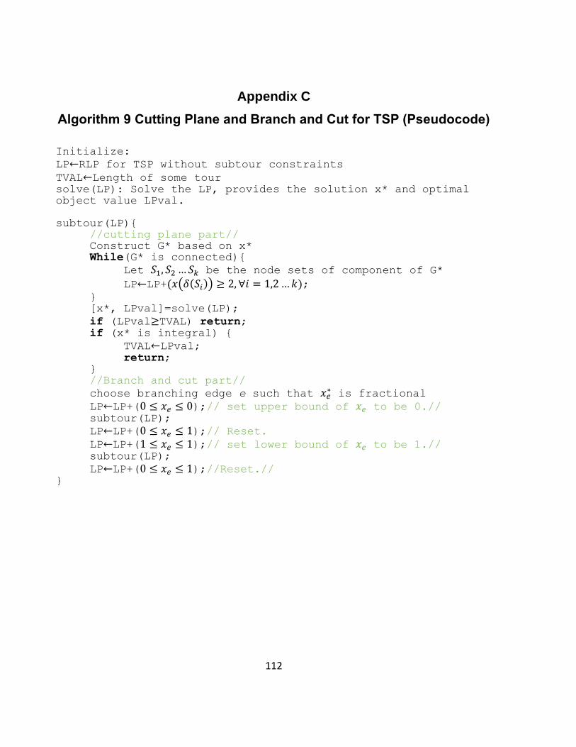
112

Appendix C

Algorithm 9 Cutting Plane and Branch and Cut for TSP (Pseudocode)

Initialize:

LP←RLP for TSP without subtour constraints

TVAL←Length of some tour

solve(LP): Solve the LP, provides the solution x* and optimal object value LPval. subtour(LP){ //cutting plane part// Construct G* based on x* While(G* is connected){

Let 𝑆1, 𝑆2 …𝑆𝑘 be the node sets of component of G*

LP←LP+(𝑥(𝛿(𝑆𝑖)) ≥ 2, ∀𝑖 = 1,2…𝑘); } [x*, LPval]=solve(LP);

if (LPval≥TVAL) return; if (x* is integral) {

TVAL←LPval;

return; } //Branch and cut part//

choose branching edge e such that 𝑥𝑒∗ is fractional

LP←LP+(0 ≤ 𝑥𝑒 ≤ 0);// set upper bound of 𝑥𝑒 to be 0.//

subtour(LP);

LP←LP+(0 ≤ 𝑥𝑒 ≤ 1);// Reset. LP←LP+(1 ≤ 𝑥𝑒 ≤ 1);// set lower bound of 𝑥𝑒 to be 1.//

subtour(LP);

LP←LP+(0 ≤ 𝑥𝑒 ≤ 1);//Reset.// }

113

Appendix D

Blossom Inequality of Cut Form

Suppose that 𝑥𝑒 is the characteristic vector for perfect matching, then

∑(𝑥𝑒 , 𝑒 ∈ 𝛾(𝑆)) ≤|𝑆| − 1

2⟺ ∑(𝑥𝑒 , 𝑒 ∈ 𝛿(𝑆)) ≥ 1.

Proof: Since 𝑥𝑒 is the characteristic vector for perfect matching, then for each 𝑆 ⊆ 𝑉, every

vertex in S should be matched. We have the following:

∑(𝑥𝑒 , 𝑒 ℎ𝑎𝑠 𝑎𝑛 𝑒𝑛𝑑𝑝𝑜𝑖𝑛𝑡 𝑖𝑛 𝑆) = |𝑆|.

Note that for each edge 𝑒 which has an endpoint in 𝑆, there are two cases:

Case1: Both endpoints of e are in S. This is the case that 𝑒 ∈ 𝛾(𝑆). In this case, two endpoints of

e are matched and they are all in S.

Case2: One endpoint of e is in S. This is the case that 𝑒 ∈ 𝛿(𝑆). In this case, only one of the

matched endpoints of e is in S

We can rewrite the left hand side, and the above equality will become to

2∑(𝑥𝑒 , 𝑒 ∈ 𝛾(𝑆)) + ∑(𝑥𝑒 , 𝑒 ∈ 𝛿(𝑆)) = |𝑆|.

Thus,

∑(𝑥𝑒 , 𝑒 ∈ 𝛿(𝑆)) = |𝑆| − 2∑(𝑥𝑒 , 𝑒 ∈ 𝛾(𝑆)) ,∑(𝑥𝑒, 𝑒 ∈ 𝛾(𝑆)) =|𝑆| − ∑(𝑥𝑒 , 𝑒 ∈ 𝛾(𝑆))

2.

If ∑(𝑥𝑒 , 𝑒 ∈ 𝛾(𝑆)) ≤|𝑆|−1

2, then ∑(𝑥𝑒 , 𝑒 ∈ 𝛿(𝑆)) ≥ |𝑆| − 2

|𝑆|−1

2= 1.

If ∑(𝑥𝑒 , 𝑒 ∈ 𝛿(𝑆)) ≥ 1, then ∑(𝑥𝑒 , 𝑒 ∈ 𝛾(𝑆)) ≤|𝑆|−1

2.

QED

114

Bibliography

[1]. http://www.redneckpoolheater.com.

[2]. John A George, Jennifer M George, and Bruce W Lamar. Packing different-sized circles

into a rectangular container. European Journal of Operational Research, 84(3):693–

712, 1995.

[3]. Q. Zhang, H.Q. Wang, W.Q. Huang and D.M. Xu. An improved algorithm for the packing

of unequal circles within a larger containing circle. European Journal of Operational

Research, 141(2):440–453, 2002.

[4]. J. O'Rourke. Finding minimal enclosing boxes. Parallel Programming, Springer

Netherlands, 1985.

[5]. W. Jiang, B. Kettlewell, T. Qiao, F. Mendivil, S. D. Peterson, and E. R. Vrscay. The

barbeque pool heater: An algorithm to construct tubular networks that occupy

arbitrary regions in r3. Applied Mathematics, Modeling and Computational Science -

Canadian Applied and Industrial Mathematics Society Congress, Waterloo, ON, June 7-

12, 2015.

[6]. W. Jiang, T. Qiao, F. Mendivil, S. D. Peterson, and E. R. Vrscay. Some novel circle-

packing algorithms devised for the construction of tubular networks in r3. Applied

Mathematics, Modeling and Computational Science - Canadian Applied and Industrial

Mathematics Society Congress, Waterloo, ON, June 7-12, 2015.

[7]. W.A. Oliveira, L.L.S. Neto, A.C. Moretti, and E.F Reis. Nonidentical circle packing

problem: multiple disks installed in a rotating circular container. arXiv preprint

arXiv:1401.4952, 2013.

[8]. H. Edelsbrunner. Algorithms in combinatorial geometry, volume 10. Springer Science &

Business Media, 1987.

http://www.redneckpoolheater.com/

115

[9]. W.H. Press; S.A. Teukolsky; W.T. Vetterling; B.P. Flannery. Numerical Recipes: The Art

of Scientific Computing (3rd ed.), New York: Cambridge University Press, ISBN 978-0-

521-88068-8, 2007.

[10]. J. Gross & J.Yellen. Handbook of Graph Theory. CRC Press, 2003.

[11]. P. Bourke. Calculating the area and centroid of a polygon, 1988.

[12]. W. Q. Huang, Y. Li, C. M. Li and R. C. Xu. New heuristics for packing unequal circles into

a circular container. Comput. Oper. Res. vol.33, pp. 2125-2142, 2006.

[13]. W.Q. Huang, Y. Li, L. Akeb, CM. Li. Greedy algorithms for packing unequal circles into a

rectangular container. Journal of Operational Research in Society, Available online doi:

10.1057/palgrave.jors.2601836, 2004.

[14]. G. B. Dantzig, R. Fulkerson, and S. M. Johnson. Solution of a large-scale traveling

salesman problem. Operations Research 2, 393-410, (1954).

[15]. M. W. Padberg and G. Rinaldi. A branch-and-cut algorithm for the resolution of large-

scale symmetric traveling salesman problems. SIAM Review 33, 60-100, (1991).

[16]. J.L. Shu, Z. Zhao, Q.Y. Dai, Genetic algorithm for TSP, Operations Research and

Management Science, Vol.13(1), 17—22, (2004).

[17]. R. César, G. Dorabela, F. Glover, C. Osterman. Traveling salesman problem heuristics:

Leading methods, implementations and latest advances, European Journal of

Operational Research, 211, issue 3, p. 427-441, (2011).

[18]. E. Scheinerman. Matgraph: A graph theory toolbox for MATLAB. [Online]. Available:

http://www.ams.jhu.edu/~ers/matgraph

[19]. N. Christofides, Worst-case analysis of a new heuristic for the travelling salesman

problem, Report 388. Graduate School of Industrial Administration, CMU, 1976.

https://en.wikipedia.org/wiki/International_Standard_Book_Number

https://en.wikipedia.org/wiki/Special:BookSources/978-0-521-88068-8

https://en.wikipedia.org/wiki/Special:BookSources/978-0-521-88068-8

116

[20]. R. Bellman. 1962. Dynamic Programming Treatment of the Travelling Salesman

Problem. J. ACM 9, 1, 61-63, January 1962.

[21]. International Business Machines Corporation, IBM ILOG CPLEX V12.1 User's Manual for

CPLEX, 2009.

[22]. J.B. Kruskal, On the shortest spanning subtree of a graph and the traveling salesman

problem". Proceedings of the American Mathematical Society 7: 48–50, 1956.

[23]. G. Reinhelt. TSPLIB: a library of sample instances for the tsp (and related problems)

from various sources and of various types. URL:

http://comopt.ifi.uniheidelberg.de/software/TSPLIB95/

[24]. W.Z. Jiang, Construction of Optimal Tubular Networks in Arbitrary Regions in R^3,

Master Thesis, University of Waterloo ,2015.

[25]. W.R. Pulleyblank, Faces of Matching Polyhedra, PhD Thesis, University of Waterloo ,1973.

[26]. Groetschel and Holland, Solving matching problems with linear programming,

Mathematical Programming 33 ,1985.

[27]. W.J. Cook, W.H. Cunningham, W.R. Pulleyblank and A. Schrijver. Combinatorial

Optimization. Wiley-Interscience ,1998.

[28]. D. Gusfield. Very simple methods for all pairs network flow analysis. SIAM J. Comput.

19, 1 143-155. DOI=10.1137/0219009, February 1990.

[29]. L.R. Ford AND D. R. Fulkerson, Flows in Networks, Princeton University Press, Princeton,

NJ, 1962.

[30]. M. W. Padberg and M. R. Rao. Odd minimum cut-sets and b-matchings. Math. Oper.

Res., 7(1):67–80, 1982.

[31]. J. Edmonds. "Paths, trees, and flowers". Canada. J. Math. 17: 449–467, 1965.

117

[32]. J. Edmonds, Maximum matching and a polyhedron with 0,1-vertices. Journal of

Research National Bureau of Standards Section B 69: 125–130, 1965.

[33]. V. Kolmogorov. Blossom V: a new implementation of a minimum cost perfect matching

algorithm. Mathematical Programming Computation, 1(1):43–67, 2009.

[34]. Laozi and S.Mitchell. Tao Te Ching: A New English Version. New York: Harper & Row,

1988.

[35]. W.J. Cook. Concorde TSP. iTunes Store. URL:

https://itunes.apple.com/ca/app/concorde-tsp/id498366515?mt=8.

[36]. E.W. Weisstein, Point-Line Distance--2-Dimensional. From MathWorld--A Wolfram Web

Resource. http://mathworld.wolfram.com/Point-LineDistance2-Dimensional.html

https://itunes.apple.com/ca/app/concorde-tsp/id498366515?mt=8

http://mathworld.wolfram.com/

http://mathworld.wolfram.com/Point-LineDistance2-Dimensional.html

design of tubular network systems using ircle packing and

Documents