design of quasi-kinematic couplings

Precision Engineering 28 (2004) 338–357

Design of quasi-kinematic couplingsMartin L. Culpepper∗

MIT Department of Mechanical Engineering, 77 Massachusetts Avenue, Room 3-449b, Cambridge, MA 02139, USA

Received 27 May 2002; accepted 16 December 2002

Abstract

A quasi-kinematic coupling (QKC) is a fixturing device that can be used to make low-cost assemblies with sub-micron precision and/orsealing contact. Unlike kinematic couplings that form small-area contacts between mating balls in v-grooves, QKCs are based on arc contactsformed by mating three balls with three axisymmetric grooves. Though a QKC is technically not an exact constraint coupling, proper designof the contacts can produce a weakly over constrained coupling that emulates an exact constraint coupling. This paper covers the practicaldesign of QKCs and derives the theory that predicts QKC stiffness. A metric used to minimize over constraint in QKCs is presented.Experimental results are provided to show that QKCs can provide repeatability (1/4�m) that is comparable to that of kinematic couplings.© 2004 Elsevier Inc. All rights reserved.

Keywords: Kinematic coupling; Quasi-kinematic coupling; Plastic deformation; Exact constraint; Fixture; Repeatability; Stiffness; Assembly; Photonics;Automotive assembly; Over constraint; Precision optics

1. Introduction

1.1. Background

The need to improve performance has forced design-ers to tighten alignment tolerances for next generationassemblies. Where tens of microns were once sufficient,nanometer/micron-level alignment tolerances are becomingcommon. Examples can be found in automotive engines,precision optics and photonic assemblies. Unfortunately, thenew alignment requirements are beyond the practical ca-pability (∼5�m) of most low-cost alignment technologies.The absence of a low-cost, sub-micron coupling has moti-vated the development of a new class of coupling interface,the quasi-kinematic coupling (QKC) (Fig. 1A).

1.2. The need for a new precision coupling

To understand the need for a new class of precision fixtures,it is necessary to understand why the cost and performancecharacteristics of current technologies are incompatible withthe dual requirements of low-cost and sub-micron precision.We will first examine coupling types used in traditionalmanufacturing. The most common type, the pinned joint, isformed by mating pins from a first component into corre-sponding holes or slots in a second component. Obtaining

∗ Tel.: +1-617-452-2395; fax:+1-509-693-0833.E-mail address: [email protected] (M.L. Culpepper).

micron-level precision with these couplings is impracticaldue to the micron-level tolerances that are required on pins,holes and pin–hole patterns. Other well-known couplingssuch as tapers, dove–tails and rail–slots would also requiremicron-level tolerances. They also require expensive fin-ishing operations to reduce the effect of surface finish onalignment performance.

Let us now consider exact constraint couplings that are wellknown in precision engineering, but less frequently used inmanufacturing. A common type of exact constraint coupling,a kinematic coupling (seeFig. 1A), routinely provides betterthan 1�m precision[1] alignment. Unfortunately, they fail tosatisfy three low-cost coupling requirements that are commonto many manufacturing processes:

1. Low-cost generation of fine surface finish: micron-levelkinematic couplings must use balls and grooves withground or polished surfaces[2]. Although balls with finesurface finish are generally inexpensive, grooves withfine surface finish are expensive. The finishing operationsused to prepare groove surfaces add considerable cost tokinematic couplings.

2. Low-cost generation of alignment feature shape: makingv-grooves for kinematic couplings requires more timeand more complicated manufacturing processes thanrequired by present low-cost technologies, i.e. pinnedjoints. For example, the ball and grooves are geomet-rically more complex, with more tolerances than pinsand holes. Likewise, high-hardness balls and grooves are

0141-6359/$ – see front matter © 2004 Elsevier Inc. All rights reserved.doi:10.1016/j.precisioneng.2002.12.001

M.L. Culpepper / Precision Engineering 28 (2004) 338–357 339

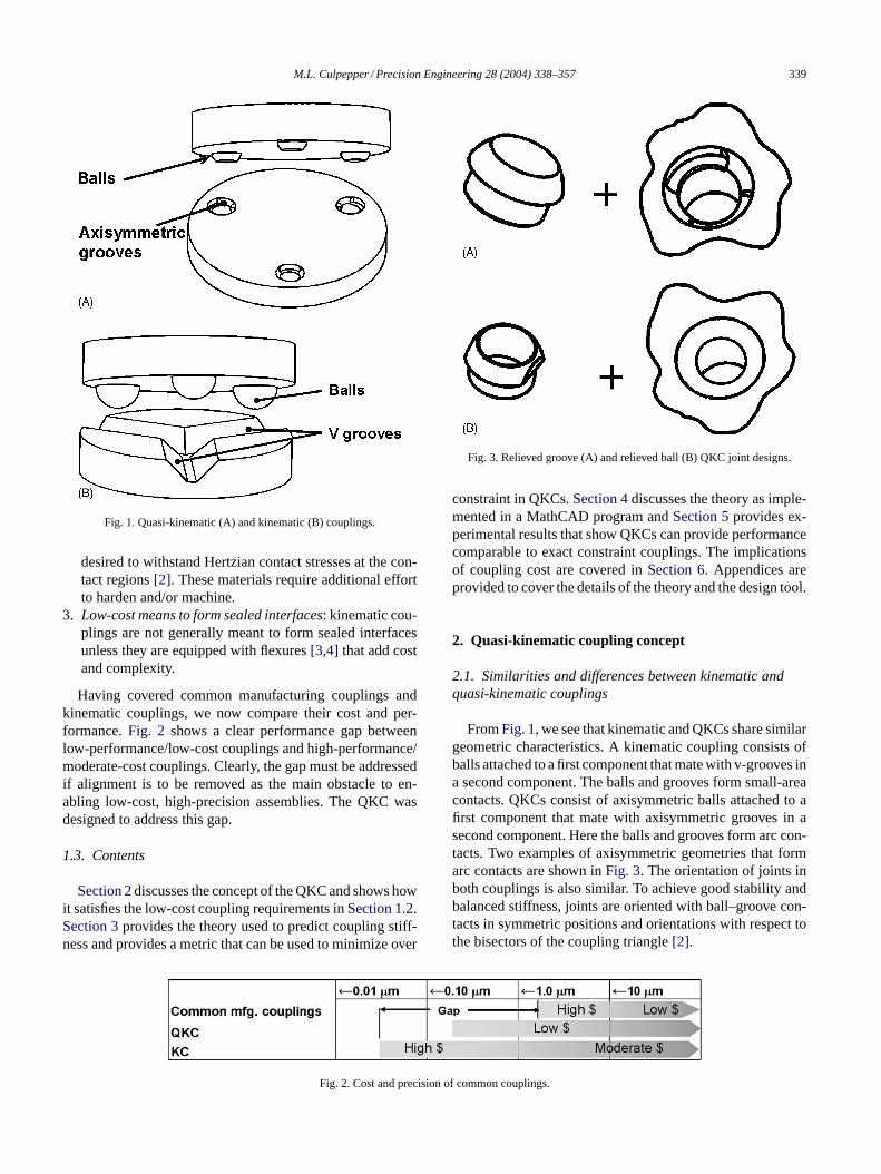
Fig. 1. Quasi-kinematic (A) and kinematic (B) couplings.

desired to withstand Hertzian contact stresses at the con-tact regions[2]. These materials require additional effortto harden and/or machine.

3. Low-cost means to form sealed interfaces: kinematic cou-plings are not generally meant to form sealed interfacesunless they are equipped with flexures[3,4] that add costand complexity.

Having covered common manufacturing couplings andkinematic couplings, we now compare their cost and per-formance.Fig. 2 shows a clear performance gap betweenlow-performance/low-cost couplings and high-performance/moderate-cost couplings. Clearly, the gap must be addressedif alignment is to be removed as the main obstacle to en-abling low-cost, high-precision assemblies. The QKC wasdesigned to address this gap.

1.3. Contents

Section 2discusses the concept of the QKC and shows howit satisfies the low-cost coupling requirements inSection 1.2.Section 3provides the theory used to predict coupling stiff-ness and provides a metric that can be used to minimize over

Fig. 2. Cost and precision of common couplings.

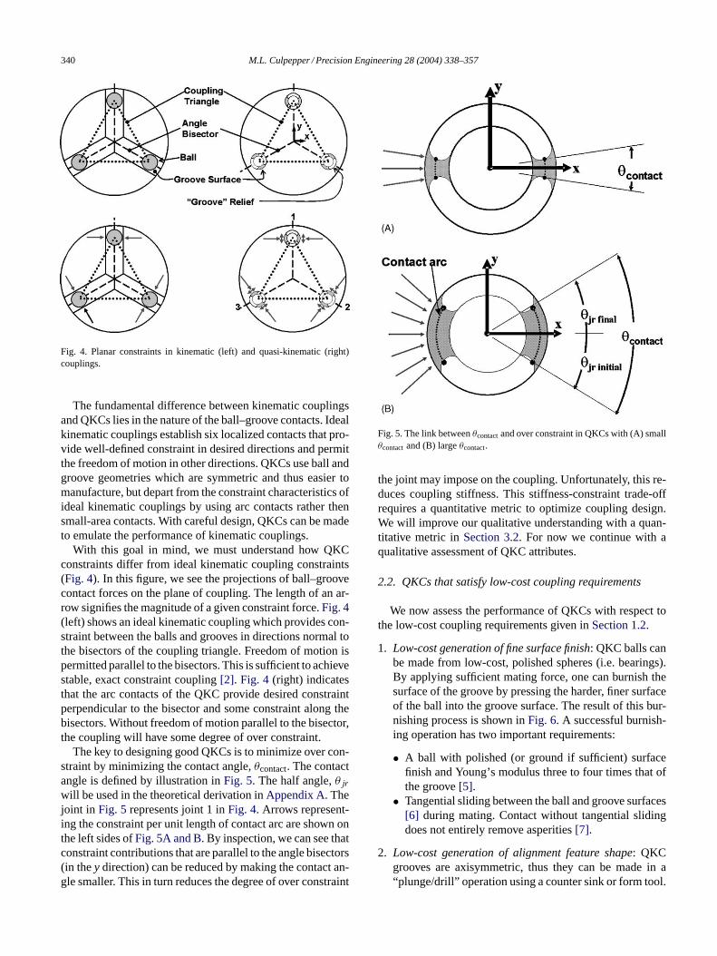
Fig. 3. Relieved groove (A) and relieved ball (B) QKC joint designs.

constraint in QKCs.Section 4discusses the theory as imple-mented in a MathCAD program andSection 5provides ex-perimental results that show QKCs can provide performancecomparable to exact constraint couplings. The implicationsof coupling cost are covered inSection 6. Appendices areprovided to cover the details of the theory and the design tool.

2. Quasi-kinematic coupling concept

2.1. Similarities and differences between kinematic andquasi-kinematic couplings

FromFig. 1, we see that kinematic and QKCs share similargeometric characteristics. A kinematic coupling consists ofballs attached to a first component that mate with v-grooves ina second component. The balls and grooves form small-areacontacts. QKCs consist of axisymmetric balls attached to afirst component that mate with axisymmetric grooves in asecond component. Here the balls and grooves form arc con-tacts. Two examples of axisymmetric geometries that formarc contacts are shown inFig. 3. The orientation of joints inboth couplings is also similar. To achieve good stability andbalanced stiffness, joints are oriented with ball–groove con-tacts in symmetric positions and orientations with respect tothe bisectors of the coupling triangle[2].

340 M.L. Culpepper / Precision Engineering 28 (2004) 338–357

Fig. 4. Planar constraints in kinematic (left) and quasi-kinematic (right)couplings.

The fundamental difference between kinematic couplingsand QKCs lies in the nature of the ball–groove contacts. Idealkinematic couplings establish six localized contacts that pro-vide well-defined constraint in desired directions and permitthe freedom of motion in other directions. QKCs use ball andgroove geometries which are symmetric and thus easier tomanufacture, but depart from the constraint characteristics ofideal kinematic couplings by using arc contacts rather thensmall-area contacts. With careful design, QKCs can be madeto emulate the performance of kinematic couplings.

With this goal in mind, we must understand how QKCconstraints differ from ideal kinematic coupling constraints(Fig. 4). In this figure, we see the projections of ball–groovecontact forces on the plane of coupling. The length of an ar-row signifies the magnitude of a given constraint force.Fig. 4(left) shows an ideal kinematic coupling which provides con-straint between the balls and grooves in directions normal tothe bisectors of the coupling triangle. Freedom of motion ispermitted parallel to the bisectors. This is sufficient to achievestable, exact constraint coupling[2]. Fig. 4 (right) indicatesthat the arc contacts of the QKC provide desired constraintperpendicular to the bisector and some constraint along thebisectors. Without freedom of motion parallel to the bisector,the coupling will have some degree of over constraint.

The key to designing good QKCs is to minimize over con-straint by minimizing the contact angle,θcontact. The contactangle is defined by illustration inFig. 5. The half angle,θjrwill be used in the theoretical derivation inAppendix A. Thejoint in Fig. 5represents joint 1 inFig. 4. Arrows represent-ing the constraint per unit length of contact arc are shown onthe left sides ofFig. 5A and B. By inspection, we can see thatconstraint contributions that are parallel to the angle bisectors(in they direction) can be reduced by making the contact an-gle smaller. This in turn reduces the degree of over constraint

Fig. 5. The link betweenθcontactand over constraint in QKCs with (A) smallθcontactand (B) largeθcontact.

the joint may impose on the coupling. Unfortunately, this re-duces coupling stiffness. This stiffness-constraint trade-offrequires a quantitative metric to optimize coupling design.We will improve our qualitative understanding with a quan-titative metric inSection 3.2. For now we continue with aqualitative assessment of QKC attributes.

2.2. QKCs that satisfy low-cost coupling requirements

We now assess the performance of QKCs with respect tothe low-cost coupling requirements given inSection 1.2.

1. Low-cost generation of fine surface finish: QKC balls canbe made from low-cost, polished spheres (i.e. bearings).By applying sufficient mating force, one can burnish thesurface of the groove by pressing the harder, finer surfaceof the ball into the groove surface. The result of this bur-nishing process is shown inFig. 6. A successful burnish-ing operation has two important requirements:

• A ball with polished (or ground if sufficient) surfacefinish and Young’s modulus three to four times that ofthe groove[5].

• Tangential sliding between the ball and groove surfaces[6] during mating. Contact without tangential slidingdoes not entirely remove asperities[7].

2. Low-cost generation of alignment feature shape: QKCgrooves are axisymmetric, thus they can be made in a“plunge/drill” operation using a counter sink or form tool.


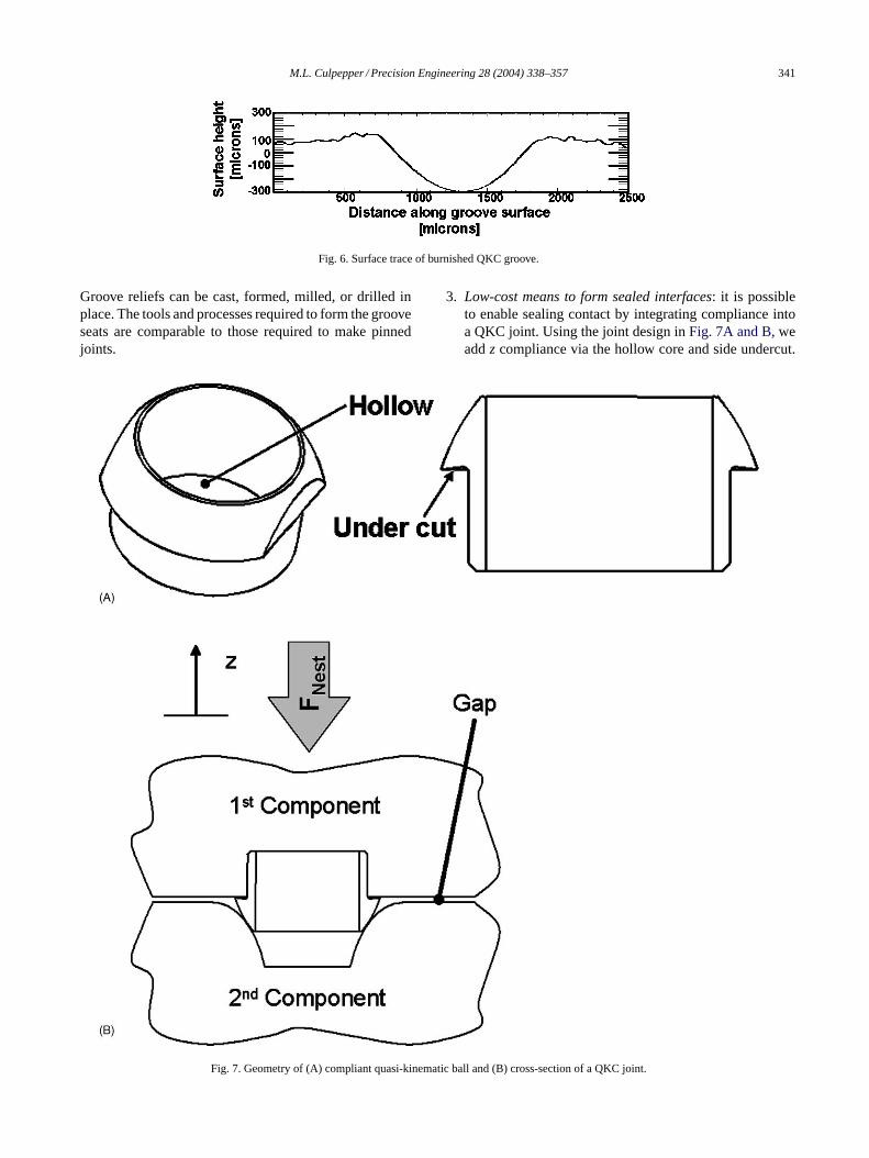
Fig. 6. Surface trace of burnished QKC groove.

Groove reliefs can be cast, formed, milled, or drilled inplace. The tools and processes required to form the grooveseats are comparable to those required to make pinnedjoints.

Fig. 7. Geometry of (A) compliant quasi-kinematic ball and (B) cross-section of a QKC joint.

3. Low-cost means to form sealed interfaces: it is possibleto enable sealing contact by integrating compliance intoa QKC joint. Using the joint design inFig. 7A and B, weaddz compliance via the hollow core and side undercut.


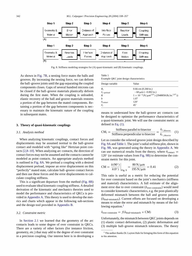
Fig. 8. Stiffness modeling strategies for (A) quasi-kinematic and (B) kinematic couplings.

As shown inFig. 7B, a nesting force mates the balls andgrooves. By increasing the nesting force, we can deformthe ball–groove joints until the gap separating the coupledcomponents closes. Gaps of several hundred microns canbe closed if the ball–groove materials plastically deformduring the first mate. When the coupling is unloaded,elastic recovery of the ball and groove materials restoresa portion of the gap between the mated components. Re-taining a portion of the gap between components is nec-essary to maintain the kinematic nature of the couplingin subsequent mates.

3. Theory of quasi-kinematic couplings

3.1. Analysis method

When analyzing kinematic couplings, contact forces anddisplacements may be assumed normal to the ball–groovecontact and modeled with “spring like” Hertzian point con-tacts[2,8–10]. When analyzing arc contacts, the direction ofcontact forces may not be assumed and the contacts cannot bemodeled as point contacts. An appropriate analysis methodis outlined inFig. 8A. We preload a coupling with a desireddisplacement preload, impose an error displacement on this“perfectly” mated state, calculate ball–groove contact forcesand then use these forces and the error displacements to cal-culate coupling stiffness.

This is a significant departure from the method (Fig. 8B)used to evaluate ideal kinematic coupling stiffness. A detailedderivation of the kinematic and mechanics theories used tomodel the performance and characteristics of QKCs is pro-vided inAppendix A. This theory is used to develop the met-rics and charts which appear in the following sub-sectionsand the design tool provided inAppendix B.

3.2. Constraint metric

In Section 2.1we learned that the geometry of the arccontacts leads to some degree of over constraint in QKCs.There are a variety of other factors (for instance friction,geometry, etc.) that may add to the degree of over constraintin a precision coupling. Our interest here is in developing a

Table 1Example QKC joint design characteristics

Design variable Value

Rc 0.66 cm (0.260 in.)δz-preload −60�m (−0.002 in.)K 1 × 10−2(N/�m2.07) (2948850(lb/in.2.07))b 1.07θcontact 120◦θc 45◦

means to understand how the ball–groove arc contacts canbe designed to optimize the performance characteristics ofa quasi-kinematic joint. We will use the constraint metric asdefined inEq. (1).

CMi = Stiffness parallel to bisector

Stiffness perpendicular to bisector= ki ||Bisector

ki⊥Bisector

(1)

Let us consider the relieved groove joint design described byFig. 9AandTable 1. The joint’s radial stiffness plot, shown inFig. 9B, was generated using the theory inAppendix A. Wecan use numerical results from the theory, whereθcontact =120◦ (or estimate values fromFig. 9B) to determine the con-straint metric for this joint.

CM = k(90◦)k(0◦)

∣∣∣∣Fig.9

= 80 N/�m

195 N/�m= 0.41 (2)

This ratio is useful as a metric for reducing the potentialfor over constraint based on the joint’s mechanics (stiffnessand material) characteristics. A full estimate of the align-ment error due to over constraint (δover constraint) would needto consider kinematic characteristics, e.g. the post-plasticallydeformed mismatch between the ball and groove patterns(δfinal-mismatch). Current efforts are focused on developing ameans to relate the error and mismatch by means of the fol-lowing equation.1

δover constraint= f(δfinal-mismatch× CM) (3)

Unfortunately, the mismatch between QKC joints depends on(1) elastic contact deformation, (2) plastic deformation and(3) multiple ball–groove mismatch tolerances. The theory

1 The author thanks Dr. Layton Hale for bringing this form of this equationto his attention.


Fig. 9. Example QKC relieved groove (A) orientation and (B) stiffnessfor θc = 45◦; θcontact = 120◦; K (N/�m2.07) = 1 × 10−2; b = 1.07;Rc = 0.66 cm;δz-preload= −60�m.

capable of describing the final mismatch has yet to be devel-oped. We will continue with the mechanics-based constraintmetric as this is immediately useful as a key element in min-imizing the potential for over constraint during the designprocess.

3.3. Making use of the constraint metric

In QKCs, the CM is unity forθcontact= 180◦ (gross overconstraint) and approaches 0 asθcontact→ 0◦. The desire toemulate exact constraint couplings compels us to specify thelowest possible contact angle. It is clear however, that one cannot specifyθcontact∼ 0◦ and obtain a coupling with reason-able stiffness. The key is simultaneous consideration of theconstraint metric and the coupling’s stiffness in directions ofinterest. We will demonstrate this approach via a hypotheti-cal application.

Consider a 120◦ coupling (grooves spaced at 120◦) thatmust resistz moments about its’ centroid. The design callsfor 125 N/�m as the lowest value for the maximum radialstiffness of a joint (Krmax would be 195 N/�m inFig. 9B). The

Fig. 10. Comparing performance metrics of QKCs.

plot in Fig. 10shows the effect ofθcontacton our constraintmetric and coupling stiffness. Given this plot, we could justifychoosing a contact angle as low as 60◦ with a CM = 0.10. Itis interesting to note that the trade-off between stiffness andconstraint is a favorable transaction at large contact angles.

4. Testing the MathCAD model

The theory developed inAppendix Awas implemented inthe MathCAD program provided inAppendix B. The modelwas checked by running the following tests:

• Imposed translation errors in thez direction produced onlynetz forces.

• Imposed rotation errors about thez axis of the couplingcentroid produced onlyz moments.

• Imposed displacements along one bisector of a 120◦ cou-pling (i.e. in they direction for the coupling inFig. 4) didnot produce nety or z moments.

• Thex andy reaction forces are 0 whenθc is 90◦ (groovebecomes a flat).

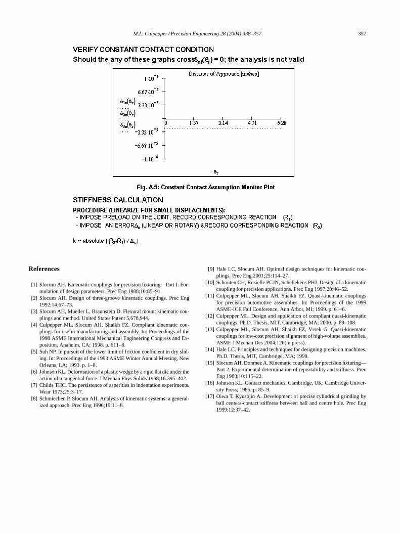
• When given inputs that would make the ball loose contactwith the groove, the model detects this as a violation ofa “constant contact” constraint (seeAppendix B, “VerifyConstant Contact Condition”).

5. Experimental results

A form of QKC has been used in precision automotive as-semblies to provide 2/3�m repeatability in journal bearingassemblies[11–13]. To meet unusual stiffness requirements,the joints were not placed in the orientations that best emulateexact constraint couplings. These joints were also designedwith large contact angles (θcontact= 120◦, CM = 0.41) to in-crease coupling stiffness. Though this design serves as proofof sub-micron performance, it is not a good means to demon-strate the best performance of QKCs.

An experiment was run to determine how repeatability ofa QKC would compare to that of an ideal kinematic coupling


when the QKCs contact angle and joint orientations were setto better emulate an ideal kinematic coupling.Table 1liststhe characteristics for the joints used in the experiment. Forthe test, the contact angle,θcontact, was set to 60◦ and thusthe constraint metric as read fromFig. 10is 0.10. This jointdesign retains the low-cost attributes of the quasi-kinematicjoint used in[11–13]and is closer in constraint characteristicsto ideal kinematic couplings and kinematic couplings withflexures[10,14].

The test coupling inFig. 11A was manufactured withless than 25�m mismatch between the axis of symmetry ofany ball and mated groove. The results of repeatability testswith lubricated joints are provided inFig. 11B. The resultsshow the coupling repeats in-plane to 1/4�m after an initial

Fig. 11. QKC (A) test setup and (B) repeatability results forθc = 32◦; θcontact= 60◦; K (N/�m2.07) = 1 × 10−2; b = 1.07;Rc = 0.66 cm; 25 N preload.

wear-in period. When this wear-in period is not practical,one may use a preload which induces plastic deformation ofthe ball–groove surfaces. This has been shown to eliminatethis wear in period and eliminate the mismatch between balland groove patterns[12]. These results compare more fa-vorably with the sub-micron performance (0.10�m) of welldesigned and lubricated kinematic couplings[15].

6. Coupling cost

The QKC elements used in the automotive assemblies andtest coupling resemble the elements shown inFig. 3A. Theseball–groove sets cost approximately $1 when manufactured


in volumes greater than 100,000 couplings per year. Whenmanufactured in volumes of less than several hundred peryear, a ball–groove set may cost $60. This is in contrast toseveral hundred dollars one could pay for high-performancekinematic couplings. In addition to the initial cost savings,the reduced replacement cost for the balls and grooves canprovide long-term cost savings.

7. Conclusions and issues for further research

This paper has provided the theory and a mechanics-basedmetric that can be used by designers to minimize the degreeof over constraint in QKCs. The theory used to model cou-pling stiffness has been implemented in MathCAD and tested.Experimental results show that properly designed QKCs canprovide precision alignment that is comparable to kinematiccouplings. Characteristics such as low-cost, ease of manufac-ture, ability to form sealed joints and sub-micron performancewill make the coupling an enabling technology. This willbe particularly important for high-precision, high-volume as-semblies in automotive, photonics, optical and other generalproduct assemblies. Subsequent research activities will in-clude developing the means to estimate alignment errors dueto the kinematic effects that result from mismatch betweenball and groove patterns.

Acknowledgments

This work was sponsored by the Ford Motor Company. Theauthor wishes to thank them for their financial and technicalassistance.

Appendix A. Theory of quasi-kinematic couplings

The purpose of this appendix is to provide the steps in aderivation of the kinematic and mechanics theories used tomodel the performance characteristics of QKCs.

A.1. Step 1: material and geometry characteristics

The first step is to identify the materials which the cou-pling components are made of and how they will be shaped

Fig. 13. Geometry characteristics of QKCs.

Fig. 12. Elastic–plastic behavior of 12L14 steel.

and arranged. We will assume common materials, shapes andsizes between the balls and grooves in the three joints.

A.1.1. Material characteristicsThe Young’s modulus and Poison’s ratio of the ball and

groove materials are needed to model elastic contact[16].Modeling plastic deformation requires a tangent modulus andstress value (yield stress) up to which the Young’s modulusmay be used.Fig. 12shows the values fitted to data from testson leaded steel.

A.1.2. Geometric characteristicsWith the help ofFigs. 13 and 14, we define important

geometry characteristics of QKCs. The first is the couplingcoordinate system, CCS, which is attached to the couplingcentroid of the grounded component (contains grooves). Adisplaced coordinate system, DCS, is attached to the centroidof the component that is displaced (contains balls) whencoupling errors are present. When the coupling is mated witha preload displacement and no error motions, the CCS andDCS are coincident.

Our analysis will now utilize subscriptsi andj to refer tospecific joints (i = 1 to 3 ) and contact arcs (j = 1 to 6),respectively. We define a joint coordinate system, JCSi, for


Fig. 14. Geometry characteristics of quasi-kinematic coupling joints.

each joint. Each JCSi measures position inri, θri, andzi ascollectively shown byFigs. 13 and 14. The z axis of eachJCSi is perpendicular to the coupling plane and coincidentwith the respective groove’s axis of symmetry. For each JCSi,θri = 0 when the projection of the joint’sr vector on thex–y plane of the CCS is parallel to thex axis of the CCS.We define a contact cone as the surface which contains alllines that run through the joint’s axis of symmetry and istangent to the ball and groove surfaces at contact. The coneis characterized by the half-cone angle,θc. Other variablesthat describe the size and location of coupling componentsare defined by illustration inFigs. 13 and 14.

A.2. Step 2: imposed error motions

Ball–groove reaction force (therefore coupling stiffness)is a function of the compression of ball and groove material.This in turn depends on the error displacement of a ball’s farfield point, SIi in Figs. 14 and 15, from its preloaded posi-tion in the groove. The displacement of a ball’s SI can be ex-pressed as a combination of the translation (δ

⇀

c) of the DCSrelative to the CCS and rotation (ε

⇀) of the displaced com-

ponent about a specified point (xε, yε, zε). This displacementcan also be given as a combination of preload displacement

Fig. 15. Positions and motions of ball and groove far field points.

and error displacement of a ball’s SIi relative to the CCS.Eq.(A.1) expresses both possibilities:

⇀

δ SIi + ⇀

δ

∣∣∣∣preloadSIi

= ⇀

δ

∣∣∣∣errorSIi

=⇀

δ c + ⇀ε × ⇀

r iε

=

δSIix i

δSIiy j

δSIiz k

(A.1)

In developingEq. (A.1), we assume the coupling is built tolimit rotation errors on the order of several microradians, thussmall-angle approximations are valid. We also assume thatgood coupling design practices have been followed so that thecoupled components can be considered as rigid bodies. Therigid body assumption requires that the mated componentsand their interfaces with the balls and grooves are more than10 times as stiff as the ball–groove contacts.

A.3. Step 3: distance of approach between far field pointsin ball–groove joints

The compression of ball and groove material may varyabout the arc contact. For example, consider a sphere mated


in a cone. If we displace the sphere into and along thecone’s axis of symmetry the compression about the resultingcircular contact will be uniform. Subsequent displacementperpendicular to the axis of symmetry will lead to variationsin compression about the contact. As reaction force dependsupon the compression of material, we expect the force per unitlength of contact arc will vary about the ball–groove contact.

A common metric used to describe material compressionbetween contacting elements is the distance of approach,δn,between two far field points[12].Fig. 15shows the distance ofapproach (asδn(θri)) between far field points, SIi andGi(θri),in a cross-section through a joint cut atθri. The distance ofapproach in a cross-section is a function of the axial (δ

⇀

SIiz)and radial (δ

⇀

r (θri)) displacement of the SIi relative to theJCSi. Eq. (A.2)provides the axial and radial displacementsas a function of ball displacement.[δr(θri) r

δSIiz k

]

=[(δ2SIix

+ δ2SIiy)0.5 cos[θri − atan(δSIiy/δSIix)] r

δSIiz k

]

(A.2)

UsingFig. 15andEq. (A.2)we can produce the relationshipfor δn(θri) given inEq. (A.3).

⇀

δ n (θri) ={−(δ2SIix + δ2SIiy)

0.5 cosphantom

(δSIiy

δSIix

)[θri − atan

(δSIiy

δSIix

)]cos(θc)+ δSIiz sin(θc)

}n

(A.3)

A.4. Step 4: modeling interface forces as a function of δn

For solid ball–groove joints that experience elastic contactdeformation, one may use classical line contact solutions torelate the distance of approach to the force per unit length ofcontact,f

⇀

n (θri) [15,17]. A more general, flexible approachis needed to model a wide range of contact situations. For in-stance, consider situations with only elastic contact deforma-tion, with contact deformation in combination with integralcompliance, or with elastic and plastic contact deformation.Practical applications that use one or more of these contactsituations were discussed inSection 2.2. Given the materialproperties and geometry characteristics from step 1, we canobtain the relationship betweenf

⇀

n (θri) andδ⇀

n (θri). Thiscan be accomplished using classical line contact solutions,FEA, or other suitable analyses from which results can be fitto the form ofEq. (A.4).

⇀

f n (θri) = K[δn(θri)]bn (A.4)

In Eq. (A.4), K is a stiffness constant and the exponentb isused to reflect the rate of change in contact stiffness withchangingδ

⇀

n (θri). BothK andb are functions of ball–groove

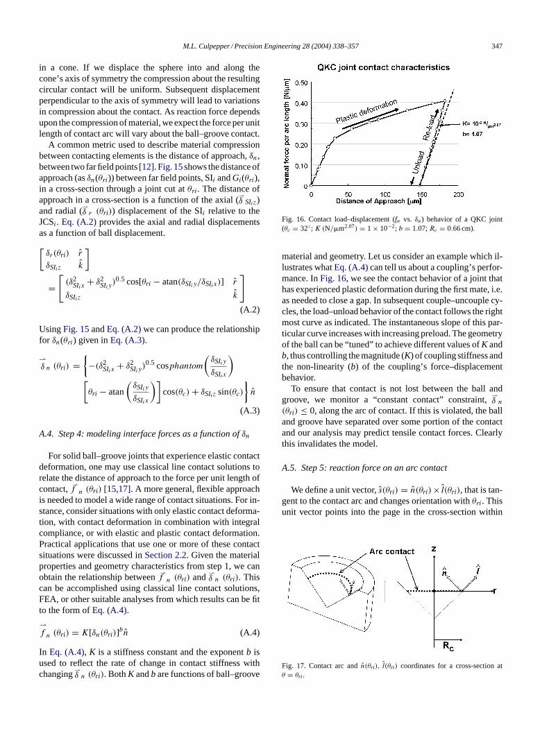
Fig. 16. Contact load–displacement (fn vs. δn) behavior of a QKC joint(θc = 32◦; K (N/�m2.07) = 1 × 10−2; b = 1.07;Rc = 0.66 cm).

material and geometry. Let us consider an example which il-lustrates whatEq. (A.4)can tell us about a coupling’s perfor-mance. InFig. 16, we see the contact behavior of a joint thathas experienced plastic deformation during the first mate, i.e.as needed to close a gap. In subsequent couple–uncouple cy-cles, the load–unload behavior of the contact follows the rightmost curve as indicated. The instantaneous slope of this par-ticular curve increases with increasing preload. The geometryof the ball can be “tuned” to achieve different values ofK andb, thus controlling the magnitude (K) of coupling stiffness andthe non-linearity (b) of the coupling’s force–displacementbehavior.

To ensure that contact is not lost between the ball andgroove, we monitor a “constant contact” constraint,δ

⇀

n

(θri) ≤ 0, along the arc of contact. If this is violated, the balland groove have separated over some portion of the contactand our analysis may predict tensile contact forces. Clearlythis invalidates the model.

A.5. Step 5: reaction force on an arc contact

We define a unit vector,s(θri) = n(θri)× l(θri), that is tan-gent to the contact arc and changes orientation withθri. Thisunit vector points into the page in the cross-section within

Fig. 17. Contact arc andn(θri), l(θri) coordinates for a cross-section atθ = θri.


Fig. 17. In Eq. (A.5)we calculate the resultant force on thearc contact via a line integral along the arc of contact.

⇀

Fj =∫ sfinal

sinitial

[fn(θri)n(θri)+ fl(θri)l(θri)+ fs(θri)s(θri)] ds

≈∫ θjr final

θjr initial

[fn(θr)n(θri)]Rc dθri (A.5)

The limits of the integral are defined by the ends of the arccontact as illustrated inFig. 5B. The subscriptsn, l, andsdifferentiate between unit contact forces in the subscripteddirections. It is good design practice to minimize friction(µstatic< 0.10) at a coupling’s contacts to prevent tangentialstress build up. InEq. (A.5)we have assumed this practice inQKC design and take the contribution of the tangential con-tact forces (in thel ands directions) as negligible comparedto the contribution of the normal forces. If a rare applica-tion requires the tangential components, they can be addedto the analysis. UsingEqs. (A.4) and (A.5)simplifies toEq. (A.6).

⇀

Fj=∫ θjr final

θjr initial

{K[δn(θri)]bn(θri)}Rc dθri (A.6)

We now use the matrix inEq. (A.7) to transform the unitcontact force into the frame of the CCS.n(θri)

s(θri)

l(θri)

=

−cos(θri) cos(θc) −sin(θri) cos(θc) sin(θc)

−sin(θri) cos(θri) 0

cos(θri) sin(θc) sin(θri) sin(θc) cos(θc)

×

i

j

k

(A.7)

In combining Eqs. (A.6) and (A.7)we obtainEq. (A.8)which provides the total reaction force for contact arcj:

⇀

Fj=

∫ θjr finalθjr initial

{Rc K(δn(θri))b[−cos(θri) cos(θc)] dθri} i∫ θjr final

θjr initial{Rc K(δn(θri))

b[−sin(θri) cos(θc)] dθri} j∫ θjr finalθjr initial

{Rc K(δn(θri))b[sin(θc)] dθri} k

(A.8)

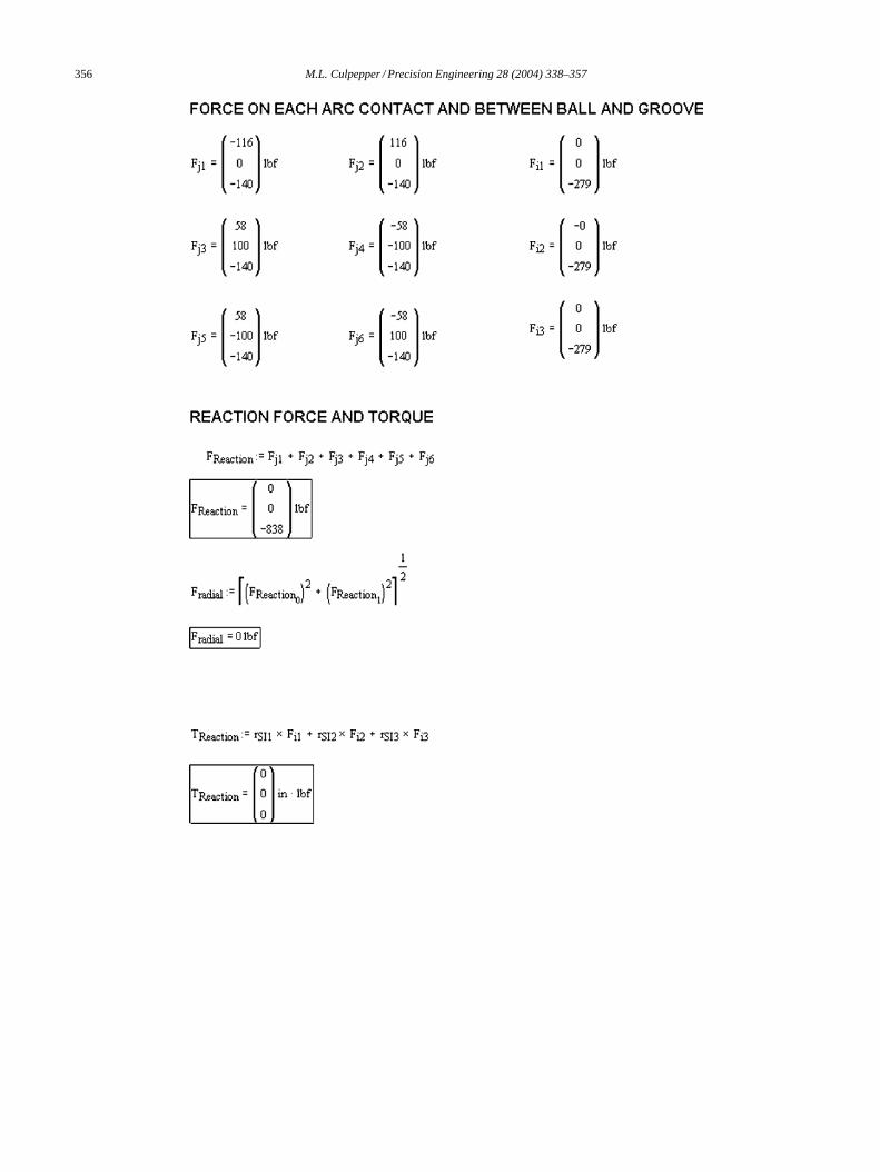
When the contact forces are summed over six contact arcs asin Eq. (A.9), we obtain the reaction force between the matedcomponents.

⇀

FReaction=6∑j=1

⇀

Fj (A.9)

The reaction torque inEq. (A.10)is the sum of torques aboutthe coupling centroid due to each ball–groove reaction force(F⇀

i) and moment arm (r⇀

SIi ) between the CCS and the re-spective ball’s SIi.

⇀

T Reaction=3∑i=1

⇀r SIi × ⇀

Fi (A.10)

A.6. Step 6: stiffness calculation

After specifying a preload displacement, the coupling stiff-ness in the direction of the error displacement is calculatedby dividing the change in reaction forces by the magnitudeof the error displacement:

kimposed= d(Reaction)

d(Imposed error displacement)(A.11)

When we apply linear displacements, the reaction is the forcegiven byEq. (A.9). When we apply rotation displacements,the reaction is the torque given byEq. (A.10).

Appendix B. Theory implemented in MathCADprogram

The MathCAD program discussed inSection 4is ap-pended for inspection. The tool is available for download athttp://psdam.mit.edu.

http://psdam.mit.edu


References

[1] Slocum AH. Kinematic couplings for precision fixturing—Part I. For-mulation of design parameters. Prec Eng 1988;10:85–91.

[2] Slocum AH. Design of three-groove kinematic couplings. Prec Eng1992;14:67–73.

[3] Slocum AH, Mueller L, Braunstein D. Flexural mount kinematic cou-plings and method. United States Patent 5,678,944.

[4] Culpepper ML, Slocum AH, Shaikh FZ. Compliant kinematic cou-plings for use in manufacturing and assembly. In: Proceedings of the1998 ASME International Mechanical Engineering Congress and Ex-position, Anaheim, CA; 1998. p. 611–8.

[5] Suh NP. In pursuit of the lower limit of friction coefficient in dry slid-ing. In: Proceedings of the 1993 ASME Winter Annual Meeting, NewOrleans, LA; 1993. p. 1–8.

[6] Johnson KL. Deformation of a plastic wedge by a rigid flat die under theaction of a tangential force. J Mechan Phys Solids 1968;16:395–402.

[7] Childs THC. The persistence of asperities in indentation experiments.Wear 1973;25:3–17.

[8] Schmiechen P, Slocum AH. Analysis of kinematic systems: a general-ized approach. Prec Eng 1996;19:11–8.

[9] Hale LC, Slocum AH. Optimal design techniques for kinematic cou-plings. Prec Eng 2001;25:114–27.

[10] Schouten CH, Rosielle PCJN, Schellekens PHJ. Design of a kinematiccoupling for precision applications. Prec Eng 1997;20:46–52.

[11] Culpepper ML, Slocum AH, Shaikh FZ. Quasi-kinematic couplingsfor precision automotive assemblies. In: Proceedings of the 1999ASME-ICE Fall Conference, Ann Arbor, MI; 1999. p. 61–6.

[12] Culpepper ML. Design and application of compliant quasi-kinematiccouplings. Ph.D. Thesis, MIT, Cambridge, MA; 2000. p. 89–108.

[13] Culpepper ML, Slocum AH, Shaikh FZ, Vrsek G. Quasi-kinematiccouplings for low-cost precision alignment of high-volume assemblies.ASME J Mechan Des 2004;126(in press).

[14] Hale LC. Principles and techniques for designing precision machines.Ph.D. Thesis, MIT, Cambridge, MA; 1999.

[15] Slocum AH, Donmez A. Kinematic couplings for precision fixturing—Part 2. Experimental determination of repeatability and stiffness. PrecEng 1988;10:115–22.

[16] Johnson KL. Contact mechanics. Cambridge, UK: Cambridge Univer-sity Press; 1985. p. 85–9.

[17] Oiwa T, Kyusojin A. Development of precise cylindrical grinding byball centers-contact stiffness between ball and centre hole. Prec Eng1999;12:37–42.

design of quasi-kinematic couplings

Documents