IEEE TRANSACI'IONS ON INFORMATION THEORY, VOL. 39, NO.3, MAY 1993 821

Design of Multiple Description Scalar Quantizers Vinay Anant Vaishampayan

Abstract-The design of scalar quantizers for communication systems that use diversity to overcome channel impairments is considered. The design problem is posed as an optimization prob­lem and necessary cOIiditions for optimality are derived. A design algorithm, a generalization of Lloyd's algorithm for quantizer design, is developed. Unlike a single channel scalar quantizer, the performance of a multiple description scalar quantizer is dependent on the index assignment. The problem of index assign­ment is addressed. Good index assignments, performance results, and sample quantizer designs are presented for a memoryless Gaussian source. Furthermore, comparisons are made against rate distortion bounds for the multiple descriptions problem.

Index Terms-Quantization, source coding, diversity systems, multiple descriptions.

1. INTRODUCTION

THE PROBLEM of scalar quantizer (SQ) design for communication systems that use diversity to overcome

channel impairments is considered. A diversity-based com­munication system (hereafter referred to as a diversity system) provides several different channels for transmitting information from the source to the user. T his way, if a channel breaks down, an alternate path is available between the source and the user. Consider a diversity system with two channels. If identical information is sent over each channel and if both channels work, half of the received information has no value. We consider sending different information over each channel in such a way that if only one channel works the information received over it is sufficient to achieve a minimum fidelity. On the other hand, should both channels work, the information from one channel can be used to augment the information from the other channel to achieve a higher fidelity than would each channel alone. The problem of designing source codes of this kind is known as the multiple descriptions problem [1] and is a generalization of the problem of source coding subject to a fidelity criterion [2].

A multiple description scalar quantizer (MDSQ) is an SQ designed for operation in a diversity system. The encoder of an MDSQ sends information over each channel of the diversity system subject to a rate constraint. The decoder reconstructs the source sample based on the information received from the channels that are currently working. The objective is to design an encoder-decoder pair that minimizes the average distortion when both channels work, subject to constraints on

Manuscript received February 14, 1992; revised August 10, 1992. This work was supported in part by NSF Grant NCR-9104566. This work was presented in part at the Joint DIMACS/IEEE Workshop on Coding and Quantization, Rutgers University, Piscataway, NJ, October 19-21, 1992. .

The author is with the Department of Electrical Engineering, Texas A&M University, College Station, TX 77843.

IEEE Log Number 9206228.

the average distortion when only one channel Works (either channel may break down). Thus, in the event that exactly one of the channels is broken, a minimum fidelity is guaranteed.

The main contribution of this paper is to present a systematic design technique as well as performance results fot the MDSQ. The design of an MDSQ consists of first selecting an index assignment and then optimizing the structure of the quantizer for the chosen index assignment. Both of these issues are addressed, for the first time, in this paper.

In [IJ, EI Gamal and Cover consider the multiple descrip­tions problem for a memory less source and a single-letter fidelity criterion. They construct an achievable rate region for the problem. Ozarow [3], by proving a converse coding theorem for the special case of a memoryless Gaussian source and the squared-error distortion criterion, has shown that the achievable rate region derived in [1], is, in fact, the rate distortion region for the source. The binary symmetric memoryless source with an error frequency distortion criterion has been studied by Berger and Zhang [4], [5], Ahlswede [6], Witsenhausen and Wyner [7], and Wolf, Wyner and Ziv [8]. It was conjectured that the achievable rate region given in [1] coincided with the rate distortion region in cases other than the Gaussian memoryless source and the squared-error distortion criterion. However, this conjecture was disproved in [5]. There have been no results to date on characterizing the rate distortion region for non-Gaussian sources and for sources with memory. An important special case of the multiple descriptions problem is the problem of successive refinement of information [9]. In [9], a necessaty and sufficient condition for a rate distortion problem to be successively refirtable is derived.

Applications of multiple des�ription source codes suggest themselves in speech and video coding over packet-switched networks where packet losses can result in a degradation in signal quality. Another possible application is communication over fading multipath channels where diversity techniques are commonly used [10]. In the context of speech coding, Jayant and Christensen [11], [12], consider a technique for combating speech quality degradation due to packet losses. Information bits corresponding to even and odd samples are placed in separate packets. If only an even (odd) sample packet is lost, data contained in the odd (even) packet is used to estimate the missing samples using nearest neighbor interpolation. The disadvaniage with this technique is that severe aliasing distortion can result when one type of packet is lost. To alleviate this problem it is necessary to either increase the sampling rate, which may not always be desirable, or to use adaptive interpolation. In contrast, the system proposed here sends information from each sample over both channels

0018-9448/93$03.00 © 1993 IEEE

822

of the diversity system. Other relevant work includes [13], where a two-channel vector quantizer is proposed for com­bating channel errors over a binary symmetric channel, and [14], where a vector quantizer design algorithm for diversity systems is presented.

This paper is organized as follows: The MDSQ design problem is formulated and notation is established in Section II. In Section III, necessary conditions for optimality are derived, based on which a design is developed. Relevant rate distortion bounds from the literature are presented in Section IV. In Section V, the index assignment problem is addressed and two index assignments are presented. Performance results are presented in Section VI and the paper is summarized in Section VII. Appendix A contains the proof of a theorem.

II. PROBLEM FORMULATION AND NOTATION Assume that we wish to encode the output of a source

which is represented by the stationary and ergodic random process {Xn' n E 1} with zero-mean and variance O"i. Our objective in this section is to describe an MDSQ and to establish notation. In order to do so, we first establish notation and terminology for a standard (single-channel) SQ.

An M-level SQ maps each source sample x to a re­construction level X, which takes values in the codebook X = {XI, X2, ... , X M }. The SQ is usually regarded as a composition of an encoder map 1 : Ii! � {I, 2, ... , M} whose output is a codeword index and a decoder map 9 : {I, 2" . . , M} � Ii!. The encoder partitions Ii! into M cells. The partition is represented by A = {AI, A2, • • • , AM} where Ai = {x: f(x) = i} , i = 1,2,'" ,M. An SQ is completely described by its partition and its codebook. Let d( x, x) be the distortion between x and X. The objective of SQ design is to select A and 9 so as to minimize E(d(X, X)).

Now assume that a diversity system has two channels, capable of transmitting information reliably at rates of R1 and R2 bits/source sample (bpss), respectively. Each channel may either be in a working or non-working state; this is not known in the encoder. The encoder sends a different description over each channel. Given the state of each channel, the source decoder forms the best estimate of the source output from the available data.

An (M1, M2)-level MDSQ maps the source sample x to the reconstruction levels xo, xl, and x2 that take values in the codebooks, io = {x?j,(i,j) E C}, Xl = {xLi E Id and X2 = {i;;,j E I2}, respectively, where II = {I, 2,· .. , Md, I2 = {I, 2" .. ,M2} and C is a subset of II x I2. Let N = ICI. An MDSQ can be broken up into two side encoders, JI: Ii! � II and h: Ii! � I2, which select the indexes i and j, respectively, and three decoders, 90: C � Ii! (central decoder), 91: II � Ii! and 92: I2 -> Ii! (side decoders), whose outputs are the reconstruction levels with indexes ij, i, and .i from the codebooks ,1'0, Xl, and ,1'2, respectively. The rate of the encoder 1m is given by Rm = log2 .lI1m bpss,l m = 1,2. The two encoders impose a partition A = {Aij, (i,j) E C} on IR, where Aij = {x: JI(x) = i, h(x) = j}. The MDSQ

I We will assume that C is selected in such a way that {,: (i, j) E C} = II and {j: (i, j) E C} = I2•

IEEE TRANSACTIONS ON INFORMATION THEORY, VOL. 39, NO. 3, MAY 1993

Fig. 1. The MDSQ in a diversity system.

is completely described by A, ,1'0, Xl, and X2. We refer to f = (JI,h) as the encoder, 9 = (90,91,92) as the decoder, to A as the central partition, and to the elements of A as the central cells.

An MDSQ, as used over a diversity system, is shown in Fig. 1. The outputs of the side encoders, i.e., the indexes i and j, are transmitted over channell and channel 2, respectively. If both indexes are received, the central decoder is used to reconstruct the source sample. On the other hand, if only i (j) is received, then side decoder 91 (92) is used to reconstruct the sample.

Let dm(x,xm) be the per-sample distortion between the source sample and the output of the mth decoder, m = 0,1, 2. We refer-to do as the central distortion and to d1 and d2 as side distortions. Let the random variable X represent the input to the MDSQ. Let the output of decoder 9m be represented by the random variable Xm, m = 0, 1,2 and let the output of JI and h be represented by random indexes I and .J, respectively. Let

A} = U A;j (1) jEI2

and let

A] = U Aij. (2) iEI,

A} (AJ) is the ith (jth) cell of the partition imposed by h (12) on Ii! We refer to the partitions generated individually by h and h as the side partitions and to their elements as the side cells. The average central and side distortions are given by

E(do(X,XO))= 2:= 1 do (x,x?j)p(x)dx , (3) (i,j)EC .4,j

and

respectively, where p(x) is the probability density function (pdf) of the source.

VAISHAMPAYAN: DESIGN OF MULTIPLE DESCRIPTION SCALAR QAUNTIZERS

For given values M1, M2, D1, and D2 an MDSQ is said to be optimal if it minimizes E(da) subject to E(d1) :S Dl and E(d2) :S D2. In this paper, we consider a special case, namely that of balanced descriptions. Two equal rate descriptions are said to be balanced if they result in identical average distortions when used individually.

III. NECESSARY CONDITIONS FOR OPTIMALITY

In this section, we derive conditions that must be satisfied by the encoder partition, A, and the decoder, g, of an optimum MDSQ, for a given set of index pairs C. Selection of C is addressed in Section V. The derivation of the necessary conditions and the design algorithm that follows are based on a Lagrangian formulation of the optimization problem. Previous work on quantizer design where Lagrangian formulations have been used include [15], [16] (entropy constrained scalar quan­tization) and [17] (entropy constrained vector quantization). The Lagrangian functional for the constrained optimization problem, L(A,g,A1,A2), is given by

L(A,g, Al, A2) = E(do(X, XO» + Al(E(dl(X, Xl» - Dl) + A2(E(d2(X, X2» - D2) . (6)

Let A* and g* be such that A* minimizes L(A, g*, AI, A2) over all A, and g* minimizes L(A*, g, Al, A2) over all g, for given Al � 0 and A2 � O. Then (A*, g*) satisfies the first-order necessary conditions [18] for minimizing E(do) subject to E(dr) :S Dl (A*, gO) and E(d2) :S D2(A*, gO). Our approach is to use an iterative descent algorithm to determine such an (A*, gO) for given values of Al � 0 and A2 � O. By varying Al and A2, a graph of the minimum average central distortion as a function of the constraints on the average side distortions will be obtained.

A. Optimum Encoder

Our objective now is to determine the encoder partition A(g, A1, A2) that minimizes L(A,g, Al, A2) for a given g, Al � 0 and A2 � O. The Lagrangian functional can be written in integral form as

(7)

where

F(X,Al,A2) = dO(X,X�'(X)h(X») + Al(d1(x,X},(X» - Dr) + A2(d2(x,XJ2(X» - D2)' (8)

For each value of x, F(x, AI, A2) can assume one of N values, one for each index pair to which x could be mapped by the encoder f. To minimize the integral it suffices to map each value of x to that index pair (i,j) for which F(x, AI, A2) is minimized. In other words, if

Aij = {x: do (x, x?j) + A1dl(x,xf) + A2d2(X,XJ) <; do (x, x?, j') + Al d1 (x, xI,) + A2d2 (x, x} ) ,

V (i',/)::j; (i,j), (i',)') E C} (9)

o '"

823

�of-------��-------------f-f------�

Fig. 2. Plots of h;j(x) for the following parameter values. x�l = -6, '0 _ 4 '0 - 2 '0 - 0 '0 - 2 '0 - 4 '0 - 6 '1 - 5 �12 _- - ,,\x� - -=-2 '�22 - "2 T�2 - "2 �3 .. - '�33 - _' Xl - � , "'2 - 0, X3 - 4, Xl - -4, x2 - 0, x3 - 0,.\, - .\2 - 4.0. Lmes correspond to, in increasing order of slope, (i,j) = (1,1), (1,2), (2,1), (2,2), (3,2), (2,3), (3,3). Note that index pairs (1,2) and (2,3) are not transmitted.

then A(g,Al,A2) = {Aij,(i,j) E C}. Note that (9) general­izes the optimum encoder condition reported in [19] and [20], and is quite similar in form.

Further simplification is possible if we assume the drr" m = 0, 1, 2 are squared -error distortion measures, i.e., dm (x, x) = (x - x)2. Define

and

(10)

,6ij = (x?Y + Al(X})2 + A2(X;)2 . (11)

Upon substituting (10) and (11) in (9) and cancelling terms, it follows that

A·· - {x' 2�··x - R .. > 2a" ·,x - R.,., 1.J - • u,1.J {J'/,J - l J fJ'l J '

V(£',)')::j; (i,j), (i',)') E C}. (12)

Let hij(x) = 2aijX - (jij' Let p,(x) = maXij hij(x). A typical set ofh;j's is illustrated in Fig. 2. Note that p,(x) is a convex, piecewise affine function of x. Hence, if hij(x) coincides with p,(x), it does so over an interval of x values. Note that it is possible that for some (i,j), hij(x) never coincides with p,(x) for any x. Such index pairs are never assigned any source sample and hence are never transmitted. We conclude that Aij is either empty or is an interval and thus the nonempty Ai/s can be characterized by their endpoints.

In order to determine the endpoints of the Ail'S (thresholds of the central partition) we begin by identifying some of the untransmitted index pairs in C. Let !3 be the remaining set of index pairs and let (i, j) E !3 if

1) for all (ii,/) E C - {(i,j)}, aij ::j; ai'j';

824

2) for all (i', j') E C - {( i, j)} for which aij = ai' j', f3ij < {3i1j';

3) for all (i', j') E C - {( i, j)} for which aij = ai' j' and f3ij = f3iljl, (j - 1)Ml + i < (j' - I)MI + i'.

Define

and

Ib = {(iii') E B: ai'j' < aiJ}, (13)

Ig = {(i',j') E B: (J'i'j' > aij} . (14)

Let t� and t� be the lower and upper endpoints of Aij. Then,

and

{ -00, tL -ij - max

(ilj')E1t

ifIt = 0, f3ij-{3i'j'

2( aij -Cii' j') ,

From (12), it follows that

B. Optimum Decoder

otherwise, (15)

otherwise. (16)

(17)

Our objective is to determine the decoder g(A, AI, A2) that minimizes L(A, g, At, A2) for a given A, At, and A2. From basic results in Bayesian estimation theory ([21, section IV.BJ), it is easy to see that the optimum decoders are given by

and

91(i) = arg min E(d1(X, y) I I = i), yEn;!

i E 'II , (18)

9o(i,j) = argminE(do(X,y) I 1= i, J = j), yEn;!

(i,j)EC, (20)

since E(do(X,XO)), E(d1(X,Xl)), and E(d2(X,X2)) are minimized simultaneously. Once again, a simplification exists in the case where di's are squared-error distortion measures. In this case, the optimum decoders are given by

91(i) = E(X I I = i), (21)

92(j) = E(X I J = j), (22)

and

9o(i,j) = E(X I 1= i, J = j), (i,j) E C, (23)

IEEE TRANSACTIONS ON INFORMATION THEORY. VOL. 39. NO. 3, MAY 1993

C. Design Algorithm

The basic design algorithm is now stated. Design Algorithm:

1) SET iteration counter l = O. Select an initial set of index pairs, C, an initial central partition A (I), and Lagrange multipliers '\1, A2 2: O. SET L(l) = 00. SET the stopping threshold {j to a suitably small value.

2) l;- (1 + 1). Determine the optimum decoder g(l) using (21)-(23), for fixed A(l-l).

3) Determine the optimum partition A (I) for fixed decoder g(l) according to the steps outlined in next algorithm.

4) Compute the Lagrangian functional, L(l), using (6). If (L(I) - L(l-ll / L(ll) < {j THEN STOP, ELSE return to step 2).

The crucial step is determining the central partition and there are several methods by which this can be done [22]. We show that determination of the central partition can be viewed as a problem of determining the extreme points of a convex set. A systematic method for obtaining the optimal central partition is described a little later in this section.

The Design Algorithm generates a nonincreasing sequence of values of the Lagrangian. Since this sequence is bounded below by zero it must converge. Note however, that the limit point could be a local minimum or even a saddle point, the final result being dependent on the initialization.

We now elaborate upon various steps in the Design Algo­rithm. Step 1), the initialization step is crucial and requires the construction of good families of index assignments. These are described in section V. Step 2), where the optimum decoder is obtained for a given encoder, is straightforward and requires no further elaboration. We now describe a method for obtaining the optimum central partition in Step 3).

Assume that the set C is known and that it contains N :<::: M1M2 index pairs. Assume that aij, f3ij, (i,j) E C are known. Our objective is to determine the upper and lower endpoints of the cell whose elements are mapped to index pair (i, j). The direct approach is to use (17). This approach can be tedious, however, and it is far simpler to pose the problem as one of obtaining the extreme points of a convex set. 2 We begin by reindexing the index pairs (i, j) E C. Let ij(l) : {I, 2" ", N} -; C, be such that l < m implies aij(l) < aij(m). For the remainder of this section, we will write at for aij(l), 131 for f3ij(/), tf for tt(I)' tV for t�(l)' U u , u U . II for Iij(I)' "1 for hij(I), and II for Iij(l)' Further, we WIll write l E C as shorthand for ij(l) E C. Let 5 = {(x,y) E [R2 : y 2: hl(x), V I E C}. 5 is a convex set, the boundary of which is {(x,IL(X)) : x E [R}, where IL(X) is defined immediately following (12). We say that hi forms a face of 5 if h/(x) = lL(x), xL :<::: x :<::: xU, for some xL and xU with xL < xU. A face hi is said to be adjacent to face hm, I f:. m, if their point of intersection lies in S. Face hi is said to lie to the left of face hm if dhl(x)/dx' < dhm(:r)/d:r: (i.e., al < am). The following facts are obvious. Index pair ij( l) is transmitted with positive probability iff hi forms a face of

2 An extreme point x of a convex set S, is one for which there do not exist distinct points of S, Xl and X2, such that x = AXI + (1 - A)X�, 0 < A < 1 [18].

VAISHAMPAYAN: DESIGN OF MULTIPLE DESCRIPTION SCALAR QAUNTIZERS

S. If hi and hm are adjacent faces of S and hi lies to the left of hm, then tV = tf;,.

Lemma 1: hI forms the leftmost face of S. Proof: Since al = mini ai, it suffices to show that hI is

a face of S. Again, since al = mini ai, it follows that for x* negative and with sufficiently large magnitude h1(x) = J1(x),

x :::; x', hence, hI is a face of S. D Theorem 1: Given that hz, I < N forms a face of S, the

following are true. a) If hz(t) = hm(t) for some t and m, m > I and

hp(t) :::; hm(t), p = 1+ 1, 1 + 2"", N, then tV = t. b) Let t satisfy the conditions of part 1 of this theorem. If

m, m > I is the largest index for which hm(t) = hz(t),

then hm forms a right adjacent face to hz.

Proof:

a) Note that If of 0 since I < N. It follows from (16) that

tV = minx: hl(X) = hp(x) . (24) p>1

Since for p > 1, the slope of hp ( .) is greater than that of hl(·), and since hm(t) � hp(t), it follows that for any x which satisfies hl(x) = hp(x), P > I that x � t. Thus, t is the minimum achieved by the right side of (24).

b) hmO is the line with the largest slope passing through ( t, hi ( t) ). Hence, there exists E > 0 such that for any x E [t, t + E), hm(x) coincides with J1(x). D

We now present an algorithm based on Theorem 1. It identifies the extreme points of the set S and hence the endpoints of the Ai/s. We refer to this algorithm as the extreme point alogrithm.

Algorithm for Determining the Extreme Points of S: 1) SET m <- 1 , p <- (m + 1), tf;, <- - 00, n <- N. 2) SET t <- (1/2)(/3m - /3p)/(am - ap). 3) Evaluate hz(t), m < I < n. SET pi <­

arg maxm < 1-::: n hl(l). If this maximum is achieved by several indexes then choose the highest index.

4) IF pi of p, SET P <- pi, n <- pi and return to step 2); ELSE, SET t� <- t, t� <- t and GO TO step 5).

5) IF P = N, STOP, ELSE, SET m <- p, p <- (m + 1), n <- N, return to step 2).

Theorem 2: The extreme point algorithm determines the endpoints of all central cells having nonzero length.

Proof" It suffices to show that the algorithm visits every face of S and for each face of S it determines the right endpoint of the corresponding central cell. We first prove that the sequence of endpoints generated by the algorithm remains unchanged if in step 4), n f--- p' is replaced by n f--- N (i.e., n is disabled). This is equivalent to proving that in step 3), arg maxm<l-:::n hl(t) = argmaxm<l hl(t). We do so by an induction on i, where i counts the number of times the algorithm has visited step 2) for a given value of m. Let t(i) be the value of t computed in step 2) at

825

the ith count. Let p( i) and p( i)' be the values of p and pi, respectively, at the ith count. For i = 1, the statement holds trivially. Assume that it holds for some i � 1. Then, hp

(i+l)(t(i» � hp

(i)(t(i»). By the induction hypothesis, since

hp(i+l) has smaller slope than hp(i)

' it follows that t(i+l) :::; t(i). Furthermore, IIlaxl>m hl(t(i+l») must occur for I that satisfies m ::; I ::; p( i + i), otherwise, hp (i+l) ( t (i)) < hi (t(i))

for some I > m, 1 of p( i + 1), which is clearly a contradiction. Next, we show that for each face that the algorithm visits, it

determines the right endpoint of the corresponding central cell correctly. Notice that with n disabled, if for a,given m, p = p' in step 4), then Theorem la) holds, and thus, the right endpoint of cell corresponding to face lim is correctly computed. For any given value of m, the algorithm must satisfy p = pI in step 4) in a finite number of steps. This is true because for a given m, in step 3), p' > p can occur only a finite number of times since pi :::; N. Finally, if for a given m, p' = p, then since the largest index was chosen in step 3), Theorem Ib) is satisfied, and hence lip' forms the right adjacent face of hm,

thus proving that the algorithm visits every face of S D

IV. RATE DISTORTION BOUNDS ON MDSQ PERFORMANCE

The multiple descriptions problem has been studied from an information theoretic perspective by several authors. El Gamal and Cover [1] assume that the source is memoryless and discrete and that the distortion measures are bounded. Their main result is as follows. Let a multiple description encoder transmit information at rates Rl and R2 bpss over each of the two channels. Let p(x, xo, xl, x2) = Pt(xO, xl, :1;21 x)Px(x) be a joint probability mass function and let

P = {p(x,XO,x\x2) : E(dt} :::; D1,E(d2):::; D2,

I(X;Xl) < Rl,I(X;X2) < R2,

I( X;XO,X1,X2) + I( X\X2) < Rl + R2}' (25)

Then, there exists an encoder-decoder pair with average central distortion no greater than Do, provided Do > infpEP E(do). This bound on the average central distortion has been evalu­ated for a memoryless Gaussian source and squ'ared-error distortion measure [1], [3]. It is shown that given Dl � 2-2R"

D2 � 2-2R2, a multiple description encoder-decoder pair operating at rates RJ and R2 exists, with E(dt} :::; Dl, E(d2) ::; D2 and with average central distortion no greater than Do, for any { 2-2(R, +R2)

2 • if II > � Do > l-(vlf-� ) ' -

2-2(R, +R2), otherwise,

(26)

where II = (1- D1)(1- D2) and � = DID2 - 2-2(R,+R2).

Conversely, in [3 J it is shown that given Dl � 2-2R• and D2 2: 2-2R2 it is impossible for a multiple description encoder-decoder pair operating at rates Rl and R2 with average side distortions that satisfy E(dl) ::; Dl and E(d2) :::; D2 to have an average central distortion smaller than the right-hand side of (26).

826

It will prove useful to interpret these results when the rates R1 and R2 are equal and high. Suppose that information is transmitted over channels 1 and 2 at the rate R bpss, but that the mse's achieved by side decoders 1 and 2 decrease at the smaller exponential rate 2(1 - atJR and 2(1 - (2)R, 0 < a2, a] -s: 1. In other words, assume that3 E(dp) � cp2-2(1-ap)R, p = 1,2. We assume, without loss of generality, that a1 -s: (12. By making appropriate substitutions in (26), it follows that, for an optimum system, E(do) � (1/c2)2-2(I+a2)R, if a1 < a2, and E(do) � (1/( JC1 + VezY)2-2(I+a)R if a1 = a2 = a. We would like the central mse to decrease at a faster exponential rate than either of the side mse' s. In order to do so, it follows from the previous discussion that it is only necessary to penalize the exponential rate of decrease of one of the side mse's. However, penalizing both the side mse's leads to a smaller coefficient for the exponential term in the expression for the central mse.

V. THE INDEX ASSIGNMENT PROBLEM

We address the index assignment problem in this section. We first formulate the problem in a slightly different way and present an example to illustrate the index assignment problem. Next, we study the behavior of the MDSQ at high rates and show that the performance of an index assignment is determined by a parameter, which we call the spread of the index assignment. We then present two families of index assignments.

Henceforth, we will work with squared-error side and cen­tral distortion measures. Since we are considering the design of balanced MDSQ's, we will assume that M1 = 1\!h = v'IVJ. We also assume that the encoded information is sent across the channels of the diversity system using fixed length codes.

Unlike the single channel quantizer design problem, the choice of the index to which each central cell is mapped determines the average distortions that the quantizer can achieve. This important aspect of the design problem is brought out by formulating it in the following manner.

Since the central cells must be intervals,4 the joint partition can be described by a vector of thresholds t = (to,t1, .. ·, tNJT, where N -s: M and to -s: t1 -s: ... -s: tN, We assum.e that [to, tN] is the support of the source pdf.s In order to complete the description of the encoder, we need to map the index I of each interval Bl = (tl-b tl] to a codeword pair (i, j) E C. The system block diagram is illustrated in Fig. 3, where a( ·) maps the interval index I to the index pair (i, j), the first and second components of which are sent over channell and channel 2, respectively. The decoders are described exactly as in the previous formulation in Section II. The design problem can now be equivalently stated as follows: minimize E(do) subject to E(d1) -s: D] and E(d2) -s: D2 over all C, t, a( ·), and g. As we shall see later, this problem is quite difficult to solve, due to the large number of possible index assignments. However, by studying

3By definition [23], f(x) � g(x) if limx-oo f(x)/g(x) = 1. 4 This was shown in Section III. S If either to or t N is infinite, the corresponding end of the interval is

assumed to be open.

IEEE TRANSACTIONS ON INFORMATION THEORY. VOL. 39, NO. 3, MAY 1993

Fig. 3. Design Algorithm.

I 11 12 21 22 I -v':l -V3/2 O. v':l/2 V3

(a)

I 11 12 22 21

-v':l -v':l/2 O. Ji/2 Ji (b)

jj 12 I 22 I I I -Ji -1/Ji I/Ji Ji

(c)

Fig. 4. Three central partitions and index assignments for a uniformly distributed source.

the problem asymptotically as the rates become high, good insights, as well as simple design criterion, can be obtained for the index assignment problem.

We first present a simple example to illustrate the index assignment problem. Assume that X is uniformly distributed over the interval (-J3 , J3) and that R 1 = R2 = 1 bpss. Consider the MDSQ designs illustrated in Fig. 4 and Tables I and II. In cases (a) and (b), each of the four codewords (1,1), (1,2), (2,1), and (2,2) is transmitted. Notice from Table II,

that case (a) is clearly superior to case (b), but that in both cases the descriptions are unbalanced and one of them is poor, i.e., it has an mse close to 1. In the third case, the codeword (2,1) is not transmitted. Here, the descriptions are balanced. The distortion achieved by the joint descriptions is larger than in cases (a) and (b), however, both descriptions individually achieve a small mse. The point of iliis example is that the central and the side mse's that can be achieved are determined by the index assignment. Whereas in this example it is easy to search through all possible index assignments, this is definitely not the case when the rates are high. In fact the total number of index assignments is L.�=l (M)!/(M - N)!.

In searching for a meaningful yet tractable criterion on which to base the index assignment, we study the exponential behavior of the central and side mse's with the transmission rate. For the remainder of this section we assume that M is large.

We start by defining the extent of the cell of a quantizer as the maximum distance between any two points contained in that cell. The definition of extent generalizes the notion of length to include cells that are formed by the union of disjoint intervals (note that side quantizer cells have this structure). Let lminp (n), p = 1,2, be the minimum value of the interval

VAISHAMPAYAN: DESIGN OF MULTIPLE DESCRIPTION SCALAR QAUNTIZERS 82?

TABLE I RECONSTRUCTION CODEBOOKS FOR FIG. 4

-0 X11

'0 X12 -0 X21 '0 "22

'1 Xl :i;� -2 Xl -2 X2

(a) -3.;3/4 -.;3/4 .;3/4 3.;3/4 -.;3/2 .;3/2 -.;3/4 .;3/4 (b) -3.;3/4 -.;3/4 .;3/4 3.;3/4 -.;3/2 .;3/2 0.0 0.0

(c) -2/.;3 0.0 2/.;3 -1/.;3 2/ .;3 -2/.;3 1/.;3

TABLE II CENTRAL AND SIDE MSE's FOR THE CENTRAL PARTITION

OF FIG. 4 AND THE CoDEHOOKS OF TABLE I

(a) (b) (c)

E(do)

1/16 1/16 1/9

E(d!)

1/4 1/4 1/3

13/16 1

1/3

index I that is mapped by a ( - ) to an index pair whose pth component is equal to n. Let lmaxp (n) , p = 1,2, be the maximum value of the interval index I that is mapped by a(.) to an index pair whose pth component is equal to n. Also define the spread sp(n) , p = 1,2 as lmaxp (n) - lminp (n) + 1. Assume for simplicity that the source pdf has finite support6 and that the source variance is unity. Let N .s; M be the number of central cells in the MDSQ and let m = 2R. In the sequel, we will use the fact that if the extent of every cell in an encoder partition? is 8(1/ Nb), 0 .s; b .s; 1, then the corresponding minimum mse is 8(1/N2b). This result is well known [24] when each cell in a partition is an interval. However, it is also true when each cell may be the union of several disjoint intervals, as is the case with the side cells of an MDSQ. This fact is proved in Appendix A.

We have available a total of M = 22R index pairs for transmission. If each of these index pairs is used (i.e., if the length of each central cell is 8(2-2R)), then E(do) will be 8(2-4R). It then follows from the rate distortion result, that either E(d1) or E(d2) must be 8(1). This case is uninteresting for the problem of finding balanced descriptions since we are looking for quantizer designs that result hi. equal and positive exponential decay rates for E(d1) and E(d2).

Let us select a subset consisting of N = 2(1+a)R index pairs, 0 .s; a .s; 1, out of the M available index pairs, and use these to encode the source. If we assume that the extent of every central cell is 8(2-(1+a)R), then the minimum E(do) will be 8(2-2(1+a)R). From rate distortion theory it then follows that the side mse's can go to zero no faster than 8(2-2(1-a)R), assuming that the descriptions are balanced. However, the actual exponential rate at which E(d1) and E ( d2) decrease is determined by the index pairs that are used for the transmission as well as the index assignment itself. The reason is that the exponential rate of decrease of the extent of each side cell is determined by the spread of its index, which in turn is determined by the index assignment. For each i and p = 1,2 let the spread sp (i ) be 8(22Rb) for some b, 0 .s; b.s; (1 +

611 should be possible to generalize the results that follow to pdf's with infinite support by a suitable limiting argument.

7By definition [23], a function g(N) is 8(J(N)) if there exist q > 0, C2 > 0 and No such that for all N > No, ellf(N)1 < Ig(N)1 < c2If(N)I.

a) /2. Then the extent of every cell of the first side partition is 8(2-R(Ha-2b»). This implies that the side mse's can decrease at a rate no greater than 8(2-2(1+iJ.-2b)R). The rate distortion results imply that 1 + a - 2b .s; 1 - a, which in turn, implies that b 2: a. Thus, rate distortion theory gives us the minimum rate of growth of the spread that any index assignment can achieve. Our objective, in searching for a good set of index pairs and an associated index assignment, is to find one for which the spread sp(i) is minimized, assuming that it is constant with respect to i and p.8

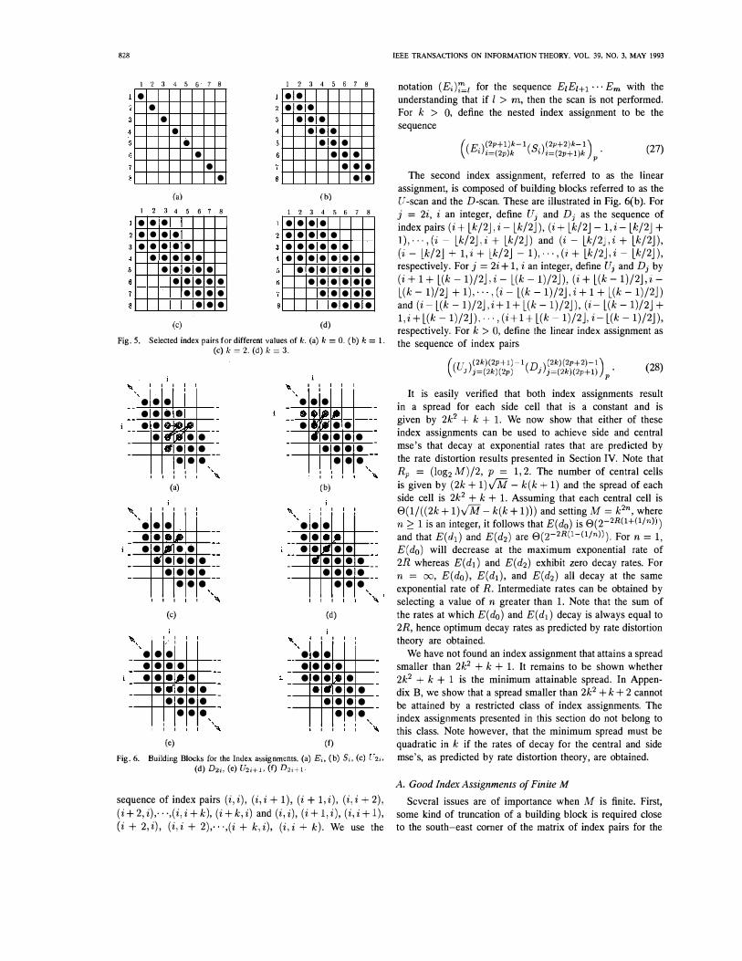
We first address the issue of selecting a set C consisting of N = 22R(1+a) index pairs. Assume that the index pairs (1,1),(2,2), .. ·,(m,m) are always among the index pairs that will be transmitted and that these index pairs will be assigned to central cells from the left to the right. Additional index pairs must first be selected so that their number is 8(22R(1+a)). Now if we had a choice between adding (1,2) and (1, m) to the set of index pairs, we would prefer (1,2) since by assigning index pairs to central cells in the order (1,1), (1,2), (2,2), (3,3),·· ·,(m, m) the maximum spread over all cells of each side partition would be 2. In contrast, if we were to have used the index pair (1, m), the maximum spread could never be smaller than r m /2l +1. If we think of an index pair as identifying an element in a m x m matrix, it becomes clear that we should exhaust all the elements that lie on a diagonal that lies closer9 to the main diagonal before moving to a diagonal that lies further away from the main diagonal. Selected index pairs for an increasing number of central cells N are illustrated in Fig. 5, for M = 64.

We now consider the index assignment problem. This can be thought of as a problem of finding a s<;anning sequence for a selected set of index pairs that results in a small spread of each cell of each side partition. We consider a set of index pairs constructed from those that lie on the main diagonal and on the 2k diagonals closest to the main diagonal. Two index assignments are first" obtained, each of which is composed of two types of basic building blocks.

The first of the index assignments, referred to as the nested index assignment, is composed of two types of building blocks illustrated in Fig. 6(a). We refer to these building blocks as the east scan (E) and the south scan (S). Each building block begins on a main diagonal element, say (i, i), visits every element of the ith row with column index no smaller than i and every element of the ith column with row index no smaller than i. More precisely, define Ei and Si as, respectively, the

8 Henceforth, we will use spread to indicate the common value of sp ( i). 9 A diagonal consisting of elements (i, i + m), i E Z is closer to the main

diagonal than the diagonal consisting of index pairs (i, i + n), i E Z if Iml< Inl·

828

2 3

1 2 3 4 5 6 7 8 •

• •

• •

• •

• (a)

1 2 3 4 5 6 7 8 ••• •• •• •• •••

•• ••• •• •• •

•• ••• •• ••

•••

(e)

1 2 3 4 5 6 7 8 •• • ••

• •• •••

••• • • •

•• • ••

(b)

1 2 3 4 5 6 7 8 • • •• • • •• • • • •• •• • • •• •••

• • •• •• • • • •• ••

•• •• • • • ••

(d)

Fig. 5. Selected index pairs for different values of k:. (a) k: = O. (b) k' = 1.

, •• •• ••

I I I I • •• • � �

• fII )I •• , . ••

•• I I I I

Ca)

I I I I I I

• •

, .

,

• •• •• •• •

•• •• ••

.� � •• •• •• •• ••

•• • I I I I

(e)

I I I I

• •• •• •

.1-•• • •• •• I I I I

(e)

•• •

Cc) k = 2. Cd) k = 3.

,

,

,

,

,

I I I I •• • . , � -. .; r-••

• •• •• • • ••

•• • I I I I (b)

I I I I

• •• •• • •

I •

.,. " •• • • •• •• ••

•• • I I I I

(d)

I I I I , • • • • • •• •• • le • . " •• •

• • •• I I I I

(f)

•• •

,

,

,

Fig. 6. Building Blocks for the Index assignments. Ca) Ei, Cb) Si, (c) U2i, (d) D2i, (e) [72i+1, (f) D2i+1.

sequence of index pairs (i,i), (i,i + 1), (i + l,i), (i,i + 2), (i + 2, i), . . ·,(i,i+k), (i+k,i) and (iii), (i+l,i), (i,i+l), (i + 2,i), (i,i + 2), . . ·,(i + k,i), (i,i + k). We use the

IEEE TRANSACTIONS ON INFORMATION THEORY, VOL. 39, NO.3, MAY 1993

notation (Ei)�Z for the sequence EzEz+!'" Em with the understanding that if I > m, then the scan is not performed, For k > 0, define the nested index assignment to be the sequence

((E-)(2p+!Jk-l (S. )(2P+2Jk-l) (27) , i=(2p)k 'i=(2p+l)k p'

The second index assignment, referred to as the linear assignment, is composed of building blocks referred to as the U -scan and the D-scan. These are illustrated in Fig, 6(b), For j = 2i, i an integer, define Uj and Dj as the sequence of index pairs (i + Lk/2J, i - Lk/2J), (i + Lk/2J -1, i -Lk/2J + l), . . ·,(i - Lk/2J,i + Lk/2J) and (i - Lk/2J,i + Lk/2J ), (i - Lk/2J + 1,i + lk/2J -1), .. ·,(i + Lk/2j,i - Lk/2j), respectively, For j = 2i + 1, i an integer, define Uj and Dj by (i + 1 + L(k -1)/2j,i - L(k -1)/2j), (i + L(k -1)/2j,i­L(k -1)/2j + 1)"", (i - L(k -1)/2j,i + 1 + L(k -1)/2j) and (i- L(k - 1)/2j,i+1+ L(k -1)/2j), (i- L(k -1)/2j + 1, i+ L(k -1)/2 j) .... , (i + 1+ L(k - 1)/2 j, i- L(k -1)/2j), respectively. For k > 0, define the linear index assignment as the sequence of index pairs

((U )(2k)(2P+!)-\D· )(2k)(2P+2)-1) (28) J j=(2k)(2p) J j=(2k)(2p+!) p'

It is easily verified that both index assignments result in a spread for each side cell that is a constant and is given by 2k2 + k + 1. We now show that either of these index assignments can be used to achieve side and central mse's that decay at exponential rates that are predicted by the rate distortion results presented in Section IV. Note that Rp = (lOg2 M)/2, P = 1,2, The number of central cells is given by (2k + 1).jM -k(k + 1) and the spread of each side cell is 2k2 + k + 1. Assuming that each central cell is 8(1/ ((2k + 1)v'M -k(k + 1») and setting M = k2n , where n:::: 1 is an integer, it follows that E(do) is 8(2-2R(1+(l/n») and that E(dl) and E(d2) are 8(2-2R(l-(I/n))). For n = 1, E(do) will decrease at the maximum exponential rate of 2R whereas E(dd and E(d2) exhibit zero decay rates. For n = 00, E(do), E(dl), and E(d2) all decay at the same exponential rate of R. Intermediate rates can be obtained by selecting a value of n greater than 1. Note that the sum of the rates at which E(do) and E(dl) decay is always equal to 2R, hence optimum decay rates as predicted by rate distortion theory are obtained.

We have not found an index assignment that attains a spread smaller than 2k2 + k + 1. It remains to be shown whether 2k2 + k + 1 is the minimum attainable spread, In Appen­dix B, we show that a spread smaller than 2k2 + k + 2 cannot be attained by a restricted class of index assignments. The index assignments presented in this section do not belong to this class. Note however, that the minimum spread must be quadratic in k if the rates of decay for the central and side mse's, as predicted by rate distortion theory, are obtained.

A. Good Index Assignments of Finite M Several issues are of importance when M is finite. First,

some kind of truncation of a building block is required close to the south-east comer of the matrix of index pairs for the

VAISHAMPAYAN: DESIGN OF MULTIPLE DESCRIPTION SCALAR QAUNTIZERS

nested index assignment and close to the north-west or the south-east comer of the matrix of index pairs for the linear index assignment. Second, it would be useful if the index assignment were such that it resulted in equal values of the average side distortion E(d1 ) and E(d2 ) when Al = A2 . Experiments with arbitrary index assignments have shown that it is extremely difficult to control the average side distortions by varying Al and A2 independently. Both issues are addressed here for the linear assignment. For the nested assignment we address only the issue of truncation close to the south-east comer of the matrix of index pairs.

We begin addressing the issue of truncation for the nested assignment. First note that 0 < k < -1M. Let ki = min(k, Viii - i) . Define Ei and Si as, respectively, the sequence of index pairs (i, i), (i, i + 1), (i + 1, i), (i, i + 2), (i+2, i) , . . . , (i, i+ki), ( i+k; , i) and (i, i), (i+ 1, i), (i, i+ 1), (i + 2, i) , (i, i + 2), . . · , (i + k;, i), (i, i + ki) . Let 'I' be the remainder obtained on dividing Viii by k and let q be the quotient. Then, if q is even, the modified nested assignment is described by

( - (2p+1)k - (2p+2)k ) qj2-1 - ,fM (Ei )i=(2P)k+1 (Si)i=(2P+1)k+1 p=O (Ei)i=,fM_1'+1 (29)

and by

( - (2p+1)k - (2p+2)k ) (q-3)j2 (Ei)i=(2P)k+1 (Si)i=(2p+1)k+1 p=o

. (E·)qk (S·) ,fM (30) ' i=(q-1)k+1 ' i=,fM -1'+1 if q is odd. We use MN(R, k) to denote the modified nested in­dex assignment that sends R bpss over each channel and which is constructed from the main diagonal and the 2k diagonals that lie closest to the main diagonal.

Now, consider the linear index assignment. We first define a truncated version of the building block for the linear index assignment, following which we address the issue of obtaining perfectly symmetric descriptions.

Consider an integer j, 2 ::::; j ::::; 2Viii (j is the sum of the components of any index pair in a given building block for the linear assignment). If j = 2i for some integer i, define kj = min(i - 1, lk/2J , Viii - i). If :j = 2i + 1 for some integer i, define kj = min(i - 1, l(k - 1)/2J , Viii - i - I). For j = 2i, define Uj by (-i + kj , i - kj ), (i + kj - 1, i ­kj + l) , . . . , (i - kj , i + kj) and 15j by (i - kj , i + kj), (i - kj + 1, i + kj - 1 ) , . . . , (i + kj, i - kj). For j = 2i + 1 define Uj by (i + l + kj , i - k), (i + kj , i - kj + l) , , , · , (i ­kj , i + kj + l) and 15.i by (i - kj , i + kj + l), (i - kj + l , i + kj) , . . · , (i + kj + l, i - kj) .

We now proceed to describe the modified linear index assignment. This index assignment, when used to initialize the design algorithm presented in Section III, results in perfectly balanced descriptions provided the following assumptions are satisfied.

1) The source pdf is symmetric about its mean value. 2) The cells of the central partition used to initialize the

design algorithm are symmetric about the mean. 3) Viii is an even integer.

1 3 1 3 5 2 4 5 2 6 8 10

6 7 9 4 7 11 12 14 8 10 11 9 13 16 17

12 13 15 15 18 21 14 16 17 20 22

18 19 21 24

20 22 (a) (b)

Fig. 7. Modified nested index assignment for (a) Jv! (b) k = 2 right.

829

19 23 25 26 28 30 27 31 32 29 33 34

64, k 1 ,

Equal side mse's are achieved by ensuring that if celi i of the first side partition consists of central cells with indexes lil , li2 , ' . . lim, then cell -1M - i + 1 of the second side partition consists of central cells with indexes N - li1 + 1, N - li2 + 1 , · · · , N - lim + 1, where the N central cells are indexed in increasing order from left to right.

Let 'I' be the remainder and q be the quotient obtained when Viii - 1 is divided by 2k. Define a = 2 + '1', b = VM + 2k + 2, and c = Viii + 2. Then, for q odd, the modified linear scan is defined by

(u . )1'+1 ((15 ) (2k)(2P+l)-1+a (u .)(2k)(2P+2) -1+a) (q-3)j2 J j=2 J 2k(2p)+a J j=(2k) (2p+1)+a p=o

(15j )�_2k+l (Viii/2, Viii/2 + l ) (Uj)���k

((D ) (2k) (2p+1) - 1+b (U . ) (2k) (2P+2)-1+b) (q-3)j2 J j=(2k)(2p)+b J (2k) (2p+1)+b p=o

- 2,fM (Dj)j=2,fM-r+1 ' (31) On the other hand, if q is even, then the modified linear index assignment is defined by

(15 r+1 ((U . ) (2k)(2P+1)- 1+a (15 .) (2k) (2P+2) - 1+a) qj2-1 J j=2 ) j=(2k)(2p)+a } (2k) (2p+1)+a p=O

(Viii/2, Viii/2 + 1)

((U ) (2k)(2P+1) - 1+C(15 ' ) (2k)(2P+2) -Hc) qj2-1 ) j=(2k) (2p)+c J j=(2k)(2p+1)+c p=o

(- )2,fM Uj j=2,fM-1'+1 ' (32)

For a given rate per channel, R bpss, we use ML( R, k) to denote the modified linear index assignment. Here again, 2k is the number of diagonals other than the main diagonal that constitute the set of transmitted index pairs.

Examples of modified nested index assignments are given in Fig. 7 and Fig. 8. Examples of modified linear index assignments are given in Fig. 9 and Fig. 10.

VI. PERFORMANCE

Performance results for the MDSQ operating on a memo­ryless, unit-variance Gaussian source have been presented for various rates and comparisons have been made against

830

1 3 5 7 1 3 5 7 9

2 8 10 12 14 2 10 12 14 16 18

4 9 15 17 19 21 4 1 1 19 2 1 23 2;' 27

6 1 1 16 22 23 25 27 6 13 20 28 30 32 34 36

13 18 24 29 30 32 34 8 15 22 29 37 38 40 42

20 26 31 36 37 39 17 24 31 39 H 45 47 28 3:3 38 41 4:3 26 3:3 41 46 49 50

:).3 40 41 44 35 43 018 51 !jl

Ca) Cb)

Fig. 8. Modified nested index assignment for Ca) M = 64, k Cb) k = 4.

3,

1 2 1 3 6

:3 4 6 2 5 7 9

5 7 8 4 8 10 12 14 9 10 I I 1 1 1 3 15 1 7 20

12 14 1 6 1 9 21 25

13 15 16 18 21 2 1 27 28 17 18 20 23 26 29 31

1 9 21 30 32 33

Ca) Cb)

Fig. 9. Modified linear index assignment for Ca) M = 64, k 1, (b) k = 2.

1 2 4 7 1 '2 4 7 1 1

3 5 8 1 1 14 3 5 8 12 16 20

6 9 12 105 18 6 9 1:1 17 21 :10

10 ]:j 16 19 21 2.l 28 10 14 18 22 25 29 :34 39

17 20 23 27 31 35 105 19 23 28 :1:1 38 4:3 22 26 30 34 38 24 27 32 :17 42 46

2" 29 3:1 37 40 2() 31 36 H 1 4.5 48 32 36 :I� 41 35 40 44 47 49

Ca) (b)

Fig. 10. Modified linear index assignment for Ca) M = 64, k = 3 (left), Cb) k = 4.

the optimum performance theoretically attainable (OPTA) as described by (26). These results are presented in Figs. 11-15. In these figures, for a given rate pair, we have plotted E(do) vs. E(d1)(= E(d2» for the ML family of index assignments and E(do) vs. (E(d1) + E(dJ))j2 for the MN family. In all cases we have set Al = A2 = A. Finally, a selected design is tabulated in Table III.

For a given rate and type of index assignment, each per­formance curve has been obtained in the following way. The parameter k has been varied from unity to its maximum value. For a given value of k, central and side mse's have been obtained for an increasing sequence {A (n) , n = 1 , 2 , . . . } with ACO) = 0 as follows. Let N(k) be the number of cells in the central partition as determined by the index assignment. The initial central partition for the quantizer design algorithm has

IEEE TRANSACTIONS ON INFORMATION THEORY, VOL. 39, NO. 3, MAY 1 993

0 _ '1J . L;j O

\ '-1

' ...... .. /

�-

E(d,)( =E(d2) Fig. 11. MDSQ performance for a unit-variance, memoryless Gaussian

source, R = 1.0 bpss. Index assignment is ML(1.0,1).

been obtained by partitioning the interval [-1 .5,1.5] into N(k) cells of equal length and indexing them according to either the modified nested index assignment or the modified linear index assignment. After the design algorithm has converged for a given A(n), the corresponding optimum MDSQ has been used to initialize the algorithm for the next value A(n+1), n = 0, 1 , · · . . A stopping threshold of 5 x 10-4 has been used for R = 1 .0, 2.0, 3.0 bpss. For R = 4.0 bpss, the stopping threshold has been set to 5 x 10-5•

For a given rate R, as A is increased, E( do) increases and E(dd (or E(d1) + E(d2)) decreases, as is expected. Also, as k is increased, lower values of the central mse are obtained since the number of central cells increases, and correspondingly, higher side mse's are obtained since the spread of the index assignment increases, Note that for a given value of k, the MDSQ obtained with A = 0 is an N(k)-level Lloyd-Max quantizer. Thus, the central mse is the same as the mse of a Lloyd-Max quantizer. The side mse, however, depends on the index assignment as we have earlier noted. For a given k, the point obtained by setting A = 0 is marked by a corresponding arrow in Figs. 11-15.

As can be seen from the results, the modified linear index assignment provides a systematic technique for trading off the central mse for the side mse. However, the central and

VAISHAMPAYAN: DESIGN OF MULTIPLE DESCRIPTION SCALAR QAUNTIZERS

0 � W

0

\ \/ k-l

." ."'2

V 0 0 OI'TA

" i:, L---��-����-'---�-�����-'-' -tJ . O l 0. 1

Fig. 12. MDSQ performance for unit-variance, memory less Gaussian source, R = 2.0 bpss. Index assignment is ML(2.0,k), k = 1 , 2 .

side mse's do not vary continuously with A. This leads to gaps in the graph of the central vs. side mse that is rather large when k = 1. This gap can be "plugged" by time­sharing.lO However, for k = 1 we have found that this gap can be plugged by deleting the index pairs (ViVi, ViVi - 1) and (ViVi + 2 , ViVi + 1) from the modified linear assignment. These assignments are designated 1* in Figs. 13 and 14.

For the modified nested assignment, the side mse's are unequal when Al = A2. The difference in the side mse's can be as large as 4 dB at low rates (R = 1, 2 bpss). While it may be possible to obtain perfectly balanced side mse's by setting Al i- A2, the search through the two dimensional parameter space is unnecessarily difficult. Consequently, we have set Al = A2 = A and have plotted only those points for which side mse's are within 0.25 dB of their arithmetic mean. As can be seen, for R = 4.0 bpss, a reasonable part of the distortion characteristic is obtained. Results for the MN family have not been presented for R = 1.0, 2.0, and 3.0 bpss since the side distortions differ by more than 0.25 dB from their arithmetic mean for a significant part of the results that we have obtained.

10 Note that logarithmic scales are used in Figs. 1 1-15, so that the points obtained by time-sharing two MDSQ's will not lie on a straight line connecting the operating points of these MDSQ's.

0 ." W

831

k=l'

"'! " j .,' 0

�I '-<."

" r '-3

� j " '-" ,r " · · J t I 2 OPrA ..

.. i:, '----��-����...L..--�-�����.....J -tJ . O l 0 . 1

Fig. 13. MDSQ performance for a unit-variance, memory less Gaussian source, R = 3.0 bpss. Index assignment is ML(3.0,k), k == 1 , 2, · · · , 6 and ML(3.0,1*).

The achievable distortion region for the ML and MN families of index assignments are almost identical except for the part of the region where k is large, i.e., small central mse and large side mse. Here, the MN family results in a smaller central mse as compared to the ML family. This is clearly because the maximum number of central cells is larger for the MN family than for the ML family.

Finally, we note that the gap between the optimnm MDSQ and the rate distortion bound is fairly large, e.g., for R = 4.0 bpss, and a given side mse, improvements of roughly 7 dB, can be obtained by designing more sophisticated codes. One such approach is to use variable length codes instead of the fixed length codes that we have used here. Another approach would be to design vector quantizers. These approaches are currently under investigation.

VII. SUMMARY

We have considered the design of multiple description scalar quantizers. The problem has been formulated as a constrained optimization problem, necessary conditions for optimality have been derived and a design algorithm has been developed_ The performance results obtained using this algorithm depend on the index assignment used. By studying the behavior of the

832

11: .. 1" I '" " i-'=1 I S \ ,-, ,-,

' 1 r \,: '-3 ,

�\J ,-, 0 ,_7 " W

, �::::" "

... OPIA I S

.. �" 11:_14

0.0 1 0. 1

Fig. 14. MDSQ performance for a unit-variance, memory less Gaussian source, R = 4.0 bpss. Index assignment is ML(4.0,k), k = 1 , 2, · · · , 14 and ML(4.0,1 *).

MDSQ's at high rates we have developed a simple criterion for index assignment selection. 1\vo index assignments have been presented. Performance results have been obtained for a memory less Gaussian source and have been compared to an available rate distortion bound from the information theory literature.

APPENDIX A

Theorem 3: Assume that source pdf pC) has finite sup­port [Xmin , xmaxl and that p has continuous first and second derivatives. Consider an MDSQ; let M = 2R and assume that it has N :::; M central cells each with length 9(1/N). Furthermore, assume that the index assignment results in a spread Nb, 0 :::; b :::; 1 for the index of each side cell. Then the side mse's go to zero as 9(1/N2(I-b) ) .

Proof: We consider E(d1), the mse of the first descrip­tion. The same result holds for E(d2) . Clearly,

itY, 2 E(dl) = L (x - xI) p(x) dx .

(i,j)EC tfj (33)

IEEE TRANSACfIONS ON INFORMATION lliEORY, VOL. 39, NO. 3. MAY 1993

1;: .. 1

J k;;2

'" I S t=4

\ �" t;;S

k;;6 0 t=7

" w \. .. I 1t::1l

S OPrA �,. '-12 -13 "'14

k=15 0 .0 1 0. 1

Fig. 15. MDSQ performance for a unit-variance, memoryless Gaussian source, R = 4.0 bpss. Index assignment is MN(4.0,k), k = 1 , 2" . . , 15.

From the mean-value theorem [18], it follows that

where Z E [ft , t�l and depends on x. From (34), it follows that

, I ( (t� - it l3 (ft - i;D3 ) p(x; )

3 - 3

1 ' 1 t'ij - Xi ij - X; ( ( U ' 1 )4 (tL ' 1 )4) + p (Xi ) 4 - 4

+ c 'J , - 'J , < d . . ( (tV - i:�)5 (tL _ i;1)5) 10 10 - 'J

< ( ' I ) ( (t� - xn3 _ (tt - xD3 )

p x, 3 3

VAISHAMPAYAN: DESIGN OF MULTIPLE DESCRIPTION SCALAR QAUNTIZERS

TABLE III OPTIMUM MDSQ DESIGN FOR A UNIT VARIANCE

GAUSSIAN SOURCE. R = 3.0 bpss.

(i,j) tb t� '0 Xij

- I Xi x;

(1, 1) -00 -2.8841 -3. 1760 -1.8300 -2.2508 (2,1) -2.8841 -2.4127 -2.6014 - 1 .4100 -2.2508 (1,2) -2.4127 -2.0904 -2 .2328 -1.8300 - 1 .2557

(3,1) -2.0904 - 1 .8540 -1.9636 -0.8342 -2.2508

(2,2) -1 .8540 - 1 .6217 -1.7306 -1 .4100 - 1 .2557

(1,3) -1.6217 - 1.4400 -1.5271 - 1 . 8300 -0.7745

(2,3) -1 .4400 - 1 .2632 -1 .3486 -1 .4100 -0.7745

(3,2) - 1 . 2632 - 1 .0930 - 1 .1757 -0.8342 -1 .2557

(2,4) -1 .0930 -0.9610 - 1 .0259 - 1 .4100 -0.4133

(3,3) -0.9610 -0 .8032 -0.8807 -0.8342 -0.7745

(4,2) -0 .8032 -0.6914 -0.7468 -0.2028 -1 .2557 (3,4) -0.6914 -5.5466 -0.6182 -0.8342 -0.4133 (4,3) -0.5466 -0.4095 -0.4775 -0.2028 -0.7745 (3,5) -0.4095 -0.3053 -0.3572 -0.8342 0.2028 (4,4) -0.3053 -0.1607 -0.2327 -0.2028 -0.4133 (5,3) -0 . 1607 -0.0718 -0 . 1 163 0.4133 -0.7745 (4,5) -0.0718 0.0718 0.0000 -0.2028 0.2028 (6,4) 0.0718 0.1607 0.1163 0.7745 -0.4133

(5,5) 0.1607 0.3053 0.2327 0.4133 0.2028 (4,6) 0.3053 0.4095 0.3572 -0.2028 0.8342 (6,5) 0.4095 0.5466 0.4775 0.7745 0.2028 (5,6) 0.5466 0.6914 0.6182 0.4133 0.8342 (7,5) 0.6914 0.8032 0.7468 1 .2557 0.2028 (6,6) 0.8032 0.9610 0.8801 0.7745 0.8342 (5,7) 0.9610 1 .0930 1 .0259 0.4133 1.4100 (7,6) 1 .0930 1 .2632 1 .1757 1 .2557 0.8342 (6,7) 1.2632 1 .4400 1.3486 0.7745 1 .4100 (6,8) 1.4400 1 .6217 1 .5271 0.7745 1 .8300 (7,7) 1.6217 1 .8540 1.7306 1 .2557 1 .4100 (8,6) 1.8540 2.0904 1 .9636 2.2508 0.8342 (7,8) 2.0904 2.4127 2.2328 1.2557 1 .8300 (8,7) 2.4127 2.8841 2.6014 2.2508 1 .4100 (8,8) 2.8841 00 3.1760 2.2508 1 .8300

ML(3,2) index assignment, .\1 =.\2 = 0.00500 , E(do) = 0.0024772, E(d1 ) = E(d2) = 0.18025, N = 33.

+ '(A l

)( (tg _ x})4

_ (tt _ xD4) P x, 4 4

+ C 'J , _ 'J , ( (tT! - x1)5 (t!- _ Xl)5 )

10 10 ' (35)

where C = minx pl/ (x) and C = maxx pl/ (x) . Since (x -a + 8)n - (x - a)n is of the same order of magnitude as 8(x - a)(n-l), it follows that each dij is 8(I/N2(1-b)+l) from which i t follows that E(d1 ) is 8(I/N2(1-bl ) . 0

APPENDIX B

In this appendix, we show that over a restricted class of index assignments the minimum spread that can be attained is given by 2k2 + k + 2, where we are assuming that the set of index pairs consists of those (i, j) for which Ij - kl � k. The index assignments presented in Section V unfortunately do not lie in this class. The proof is presented because the ideas used may tum out to be useful in proving a more general result.

The index assignment a(·) assigns to each integer l an index pair (i, j). We refer to i and j in an index pair (i, j) as the row and column number, respectively. Define sri and eri as the minimum and maximum values of I for which the row number of a(l) equals i. Define SCj and eCi as the minimum

k+I column end points k column start points ,,,'1 ...... -... -... ... �,,J� .. ...

sr· " , -,," ;.( ......... ............. ... � I " I , .. ... " ... ... ___ ..... eri , I " � � �-, I II ;,,( , ���-� t

• Column Start Point

• CoIwnn End Point

Fig. 16. A minimum spread configuration.

833

and maximum values of I for which the column number of a( I) equals j. We refer to sri and eri as the start and end points of row i, respectively. Similarly, SCj and eCj are referred to as the start and end points of column j, respectively.

The following assumptions restrict the class of index as­signments being considered. We assume that eri - sri = ec; - SCi for all i, that eri+1 - eri = sri+l - sri =

eC;+1 - eCi = SCi+l - SCi = 2k + 1, for all i. Note that . N

hmN-+oc (Li=l (eri+l - eri )/N) = 2k + 1 must be true for any index assignment.l1 The restriction we are imposing here is that equality hold for each i. The index assignments presented in Section V violate this assumption.

Theorem 4: Under the assumptions previously stated, the spread of an index assignment can be no smaller than 2k2 + k + 2.

Proof: The proof of this theorem is based on the fact that for every j for which i - k � j � i + k, either sri � SCj � eri or sri � eCj � eri, but not both. Thus, at least 2k + 1 column start/end points must lie within [sri, eriJ . Fig. 16 shows a sequence of column start and end points that are equally spaced according to our assumptions. Thus the problem of minimizing the spread of a row can be thought of as a problem of placing sri and eri in such a way that 2k + 1 consecutive column start/end points lie in [sri , eriJ. Note that the endpoint of a column (row) cannot cQincide with a start point of any column (row). Thus if the end point of column number j were to coincide with sri, then the end point of column number j', for any j' #- j cannot coincide with eri, since this would imply that the start point of column number j' must coincide with sri. But sri already coincides with eCj . Thus, a contradiction is reached. For this reason the configuration shown in Fig. 16 results in the smallest spread, which is given by 2k2 + k + 2. 0

ACKNOWLEDGMENT

The author would like to thank Prof. T. R. Fischer for a suggestion that helped improve the paper.

REFERENCES

[I] A.A. El Gamal and T. M. Cover, "Achievable rates for multiple de­scriptions," IEEE Trans. Inform. Theory., vol. IT-28, pp. 851-857, Nov. 1982.

. [2] c. E. Shannon, "Coding theorems for a discrete source with a fidelity

criterion," IRE Nat. Conv. Rec., vol. 4, pp. 142-163; Mar. 1959.

11 The same is true for the end and start points of the columns and the start points of the rows.

834

[3] L. Ozarow, "On a source coding problem with two channels and three receivers," Bell Syst. Tech. J., vol. 59, pp. 1909-1921, Dec. 1980.

[4] T. Berger and Z. Zhang, "Minimum breakdown degradation in binary source encoding," IEEE Trans. Inform. Theory, vol. IT -29, pp. 807 -814, Nov. 1983.

[5] Z. Zhang and T. Berger, "New results in binary multiple descriptions," IEEE Trans. Inform. Theory, vol. IT-33, pp. 502-521, July 1987.

[6] R. Ahlswede, "The rate-distortion region for multiple descriptions with­out excess rate," IEEE Trans. Inform. Theory, vol. IT-31, pp. 721-726, Nov. 1985.

[7] H. S. Witsenhausen and A. D. Wyner, "Source coding for multiple descriptions II: A binary source," Bell Syst. Tech. J., vol. 60, pp. 2281 -2292, Dec. 1981.

[8] J. K. Wolf, A. D. Wyner, and J. Ziv, "Source coding for multiple descriptions," Bell Syst. Tech. J., vol. 59, pp. 1417-1426, Oct. 1980.

[9] W. H. R. Equitz and T. M. Cover, "Successive refinement of informa­tion," IEEE Trans. Inform. Theory, vol. 37, pp. 269-275, Mar. 1991.

[10] J. G. Proakis, Digital Communications. New York: McGraw-Hill, 1983. [ 1 1] N. S. Jayant and S. W. Christensen, "Effects of packet losses in

waveform coded speech and improvements due to an odd-even sample interpolation procedure," IEEE Trans. Commun., vol. COM-29, pp. 101-109, Feb. 1981.

[12] N. S. Jayant, "Subsampling of a DPCM speech channel to provide two self-contained half-rate channels," Bell Syst. Tech. 1., vol. 60, pp. 501 -509, Apr. 1981.

[13] T. Moriya, "1\vo-channel conjugate vector quantizer for noisy channel speech coding," submitted to IEEE Trans. Commun.

IEEE TRANSACTIONS ON INFORMATION THEORY, VOL. 39, NO. 3. MAY 1993

[14] V. Vaishampayan, "Vector quantizer design for diversity systems," in Proc. Twenty-Fifth Ann. Con! Inform. Sci. Syst., Johns Hopkins University, Mar. 20-22, 1991, pp. 564-569.

[15] T. Berger, "Optimum quantizers and permutation codes," IEEE Trans. Inform. Theory, vol. IT-18, pp. 485-497, Nov. 1972.

[16] N. Farvardin and J. W. Modestino, "Optimum quantizer performance for a class of non-Gaussian memory less sources," IEEE Trans. Inform. Theory, vol. IT-30, pp. 485-497, May 1984.

[17] P.A. Chou, T. Lookabaugh, and R. M. Gray, "Entropy-constrained vector quantization," IEEE Trans. Acoust. Speech, Signal Processing, vol. 37, pp. 31 -42, Jan. 1989.

[18] D. G. Luenberger, Linear and Nonlinear Programming, second ed. Reading, MA: Addison Wesley, 1984.

[19] J. D. Gibson and T. R. Fischer, "Alphabet-constrained data compres­sion," IEEE Trans. Inform. Theory, vol. IT-28, pp. 443-457, May 1982.

[20] Y. Linde, A. Buzo, and R. M. Gray, "An algorit\1m for vector quantizer design," IEEE Trans. Commun., vol. COM-28, pp. 84-95, Jan. 1980.

[21] H. V. Poor, An Introduction to Signal Detection and Estimation. New York: Springer-Verlag, 1988.

[22] N. Farvardin and V. Vaishampayan, "Optimal quantizer design for noisy channels: An approach to combined source-channel coding," IEEE Trans. Inform. Theory, vol. IT-33, pp. 827-838, Nov. 1987.

[23] H. S. Wilf, Algorithms and Complexity. Englcwood Cliffs, NJ: Prentice­Hall, 1986.

[24] S. P. Lloyd, "Least squares quantization in peM," IEEE Trans. Inform. Theory, vol. IT-28, pp. 129-137, Mar. 1982.