design of hiv viral dynamics studies

STATISTICS IN MEDICINE

Statist. Med. 17, 2421—2434 (1998)

DESIGN OF HIV VIRAL DYNAMICS STUDIES

IAN C. MARSCHNER*

Department of Biostatistics and Center for Biostatistics in AIDS Research, Harvard School of Public Health,677 Huntington Avenue, Boston, MA 02115, U.S.A.

SUMMARY

HIV viral dynamics studies involve repeated measurement of viral load in HIV-infected individuals,to asses short-term rates of viral load change in response to interventions such as initiation or withdrawalof antiviral therapy. Such studies are an important source of information on HIV pathogenesis. Thispaper concerns some statistical issues arising in their design. Using a linear random-effects model toincorporate between-patient differences in rates of viral load change, I discuss the choice of number ofindividuals and frequency of observation per individual. I suggest an approach for calculating the optimalsample size and observation frequency, based on minimizing the total number of viral load measurementsthat one needs to undertake. The conclusion, using this approach, is that over a period of linear change inviral load, three to five measurements per individual is generally appropriate. I also examine the observationfrequency when the number of available individuals is limited, in which case it is shown that one can usea higher frequency of measurement per individual to achieve adequate power or precision. Finally,I consider sources of data for prior specification of variance components, together with conservative designsthat are insensitive to a lack of prior information about between-patient differences. ( 1998 John Wiley& Sons, Ltd.

1. INTRODUCTION

Current HIV research relies heavily on the measurement of viral load in HIV-infected individuals,the most common measure of viral load being the concentration of HIV RNA in plasma. Animportant class of studies dealing with HIV viral load are so-called viral dynamics studies, whichtypically consider short-term changes in viral load over time, to obtain information aboutparameters that govern HIV pathogenesis. While differing in objectives and context, viraldynamics studies have a common structure in that they use repeated measures of viral load overa short period of time to assess and compare rates of change in viral load. The present paperconcerns statistical issues in the planning of such studies, and develops some general guidelinesfor their design. To motivate the discussion we begin by considering three examples of HIV viraldynamics studies.

* Correspondence to: Ian C. Marschner, Department of Biostatistics and Center for Biostatistics in AIDS Research,Harvard School of Public Health, 677 Huntington Avenue, Boston, MA 02115, U.S.A. E-mail: [email protected]

Contract/grant sponsor: National Institute of Allergy and Infectious DiseasesContract/grant number: AI24643

CCC 0277—6715/98/212421—14$17.50 Received July 1997( 1998 John Wiley & Sons, Ltd. Accepted December 1997

Example 1: Viral decay studies. Production and clearance of HIV in vivo occurs at very highrates, with the lifetimes of individual virions and virus-producing cells being measured in daysor even hours. For much of the natural history of HIV infection, levels of detectable virusremain relatively constant, indicative of a steady-state balance between viral production andclearance. When this balance is perturbed with the use of antiviral drugs that block HIVreplication, there is a pronounced decay in the level of detectable virus. Studies have shownthat after an initial lag (1—2 days) the decay in viral load is linear on the log scale for a period ofapproximately 2 weeks.1—3 The magnitude of the decay rate is a function of the effectiveness ofthe antiviral drug (which may vary from drug to drug) and the virus production and clearancerates (which are independent of the drug). Under the assumption that the drug blocks 100 percent of HIV replication, one can use the pattern of viral decay to estimate viral production andclearance parameters. Alternatively, for non-perfect drugs, decay rates may differ betweendrugs and comparison of these decay rates yields information about the relative effectiveness ofthe drugs in blocking HIV replication.

Example 2: Viral rebound studies. Patients with suppressed levels of virus due to antiviraltherapy may experience a rebound in viral load when therapy is withdrawn. Withdrawal oftherapy may occur due to toxicity or during a washout period prior to entry onto clinical trials.More recently, clinical trials have begun to investigate so-called eradication hypotheses,where individuals with prolonged suppression of viral load may be withdrawn from therapy toinvestigate whether the virus remains suppressed or returns to former levels. In these studies,one can use repeated measures of viral load during the period directly following withdrawal oftherapy to assess the dynamics of viral rebound, if it occurs. In particular, for individuals withsuppressed viral load, the rate of increase of viral load soon after the withdrawal of therapy willbe primarily determined by the rate of production of new virus. Thus, such studies can yieldinformation about the production of virus when suppression is lost. In addition, by comparingdifferent populations (for example different CD4 count strata), such studies allow assessment ofdifferences in viral production rates.

Example 3: Viral simulation studies. Stimuli that lead to activation of the immune system, suchas influenza vaccination, are known to produce significant short-term increases in viral loadamong HIV infected individuals.4 One can use viral dynamics studies on such individuals toquantify the increased rate of viral production due to immune activation. Furthermore, suchstudies could lead to information about the mechanism by which immune stimulation increasesviral load. Plausible hypotheses are that immune stimulation increases the replication rate ofactively circulating HIV, or alternatively that immune stimulation causes previously latentlyinfected cells to become productively infected. In individuals having virus with recentlyacquired drug-resistance mutations, virus produced by latently infected cells will be wild-type,whereas virus produced by replication of actively circulating HIV will possess the resistancemutations. Thus, assessment of whether the rate of change in wild-type viral load is signifi-cantly greater among the immune activated study group (as compared to a control group),would provide a test of whether latently infected cells are being stimulated by immuneactivation. If so, quantification of the rate of increase in wild-type viral load subsequent toimmune stimulation would lead to information about the activation rate of latently infectedcells.

Owing to the expense of obtaining viral load measurements, a number of issues arise relating tothe optimal use of resources in viral dynamics studies. As early as Cox5 it was observed that the

2422 I. MARSCHNER

( 1998 John Wiley & Sons, Ltd. Statist. Med. 17, 2421—2434 (1998)

design of repeated measures studies depends on both the number of individuals and the numberof measurements per individual. More recent studies have considered the relationship betweensample size and measurement frequency in repeated measures contexts having more complexdependence structures, particularly in the presence of missing data.6,7 In the present paper weconsider in detail the trade-off between frequency of measurement and overall number ofindividuals, using a linear random effects model for change in viral load. Our goal will be toconstruct designs that balance these two quantities in an optimal way, such that the overallrequired number of viral load measurements is minimized. We also discuss a number of otherdesign issues, using the basic linear random-effects model. While more complex dependencestructures may be useful for analysing data on longitudinal measures of viral load,8,9 such modelsare likely overly cumbersome in the design stage. A linear random-effects model, however,incorporates the primary sources of viral load variability between and within individuals, while atthe same time retaining a level of tractability that is appropriate at the design stage.

2. LINEAR RANDOM-EFFECTS MODEL

In this section we describe the relationship between sample size and power for a random-effectsmodel having linear changes in viral load over time. Linearity, or piecewise linearity, is usuallya good assumption for viral load changes. None the less, depending on the context, linear viralload changes may not begin immediately subsequent to baseline. This is the case in Example 1discussed above, where inhibitors of HIV protease are used to block HIV replication. Due to theirmechanism of action they take 1—2 days to produce declines in viral load. In this case initial viralload level would technically refer to the level 1—2 days after treatment initiation, although thiswould generally be very similar to the baseline level. For the purpose of designing viral dynamicsstudies, it is unlikely that formal statistical considerations can usefully guide the sampling schemein this brief 1—2 day period. Instead, formal statistical considerations are likely most useful inguiding the sampling design during periods of linear changes in viral load, to ensure attainment ofadequate information about the rates of change. We give some further discussion of non-linearityissues in Section 5.1.

We assume that a time interval exists within which linearity of viral load change is a reasonableassumption, and that we wish to design the sampling scheme of viral load measurements in thistime interval. For the purpose of designing the study, we assume that all individuals in the samplehave viral load measurements taken at a common set of times t

1,2 , t

m. Assuming individuals

belong to one of K groups (for example, treatment arms or CD4 count strata), we denote the viralload of individual i at time t

jin group k as »(k)

ij, where each group contains n individuals.

Typically »(k)ij

is log10

of the number of HIV RNA copies per millilitre of plasma. Both initiallevels and rates of change of viral load may differ between groups. Furthermore, within groups,there may be substantial variation between individuals with respect to both initial viral load andsubsequent rates of change.10 Thus, we use the linear model

» (k)ij"c(k)

0i#c(k)

1itj#e(k)

ij.

To model variation between individuals in both initial viral load and subsequent rates of change,we assume that Me(k)

ijN are i.i.d. N(0, p2N, Mc(k)

0iN are i.i.d. N(k(k)

0, p2

0), and Mc(k)

1iN are i.i.d. N(k(k)

1, p2

1).

In addition, we assume Me(k)ij

N, Mc(k)0i

N and Mc(k)1i

N are independent of each other. The independence ofthe intercept and gradient random effects may initially appear to be a strong assumption; there isevidence, however, that this is reasonable in the present context.1,2

HIV VIRAL DYNAMICS STUDIES 2423


If the objective of the study is comparison of K"2 treatment groups, then the primary goal isto compare the average rates of change k(1)

1and k(2)

1. However, in many studies K"1, and the

primary objective is estimation of the rate of change in viral load, namely, estimation of k(1)1

. Thus,we determine the sample size and study design based on a desire to achieve specified power fora comparison of rates of change, or alternatively, specified precision for an estimate of rate ofchange. The following discussion is based on the two-sample context; however, as brieflydescribed below, it easily adapts to apply to the one-sample case. We do not explicitly considerthe case of K'2 because, from a design point of view, we would power multiple comparisonsbetween more than two groups based on a single pairwise comparison with a conservativesignificance level (for example, 0)05/C where C is the number of comparisons). Thus, study designfor K'2 would make use of the methodology for K"2.

Study design is governed by the common variance of the estimates k̂(k)1

. We obtain anexpression for this quantity by adapting the discussion of Diggle et al.11 to the present linearrandom-effects model. Let R be the m]m correlation matrix of M»(k)

ij; j"1,2, mN, which is not

dependent on the individual i nor the group k. Under the assumed linear random-effectscovariance structure, the (r, c) element of R is

orc"

p20#t

rtcp21

IM (p20#t2

rp21#p2 )(p2

0#t2

cp21#p2 )N

. (1)

Let X be the m]2 matrix

X @"C1

t1

1

t2

2

2

1

tmD .

Then the distribution of the maximum likelihood estimator k̂(k)1

is N(k(k)1

, qn), where q is the lower

right-hand entry of the 2]2 matrix p2 (X @R~1X)~1. Since q depends on the three components ofvariation (p2

0, p2

1, p2), it is necessary to have estimates of each of these to undertake inference on

Mk(k)1

N. When m*3, it is possible to estimate the three components of variation from the dataM» (k)

ijN. For m"2, we can estimate only two components, so it is necessary to use external

information about one of the components (typically p, see Section 4). Below we allow for thepossibility that m"2, although for the above and other reasons we would generally not use thisvalue.

Using the fact that ( k̂(1)1!k̂(2)

1)/I(2q/n) is standard normal, the a-level one-sided power to

detect to given difference d between k(1)1

and k(2)1

is 1!b"1!'(z1~a#dI( n

2q )), wherezx"'~1 (x). It follows that the number of individuals n in each group is given by the expression

n"2(z

1~a#z1~b)2

d2q"bq (2)

where b is a constant depending on the pre-specified significance level, power and detectabledifference.

Equation (2) shows that the sample size n is determined by the quantity q, which in turndepends on the components of variation in viral load (p2

0, p2

1, p2) and the number and timing of

measurements for each individual. Thus, if prior information is available regarding the primarysources of variation in viral load, and the number and timing of measurements per individualhave been pre-set, it is straightforward to determine the required number of individuals per groupusing (2). The number and timing of measurements might be pre-set in situations where the

2424 I. MARSCHNER


burden on patients is of great concern and overly frequent measurement cannot be carried out.However, often the number and timing of measurements per individual are not pre-set, and arechosen during the design stage of the study. Thus, one typically desires to choose simultaneouslythe overall sample size n together with the number and timing of measurements per individual.Furthermore, in some cases it may not be possible to obtain prior information about thecomponents of variation in viral load, particularly p2

1. Thus, designs robust to uncertainty about

such sources of variation are desirable. We address these issues in the following sections using thebasic relationship (2).

Before ending this section note that although the above discussion was framed in the context ofcomparing two groups with respect to change in viral load over time, we can apply the previousand following discussion to the case where we wish to estimate a single rate of change witha desired precision. In particular, if we wish to estimate k(1)

1with a 100(1!a) per cent confidence

interval having half-width w, then the relationship n"bq in equation (2) continues to hold withb"4z2

1~a@2/w2.

3. SAMPLE SIZE AND OBSERVATION FREQUENCY

In this section we consider studies in which prior information is available about the threevariability parameters, and viral load measurements are taken at equally spaced points in time.For such studies, the key quantities determining study design are the sample size (number ofindividuals) and the observation frequency (number of viral load measurements per individual).Implicit in the relationship (2) is a trade-off between the number of measurements per individual(m) and the number of individuals in each group (n). By varying n and m in opposite directions it ispossible to keep the power of the comparison constant, reflecting the fact that we can balance lowsampling frequency with a large sample size, and vice versa. Thus, since many (m, n) combinationslead to the same power, the question arises as to which combination to choose.

3.1. Optimal Observation Frequency

In view of the high cost of viral load assays, it is natural to attempt to minimize the total numberof viral load measurements that one needs to obtain N"2mn. This provides a basis for choiceamong (m, n) combinations that achieve adequate power. In particular, among all (m, n) combina-tions that achieve the desired power, the combination that minimizes N provides the optimalallocation of assay resources. We now describe this minimization problem in more detail.

For given values of a, b, d and (p, p0

, p1), the value of m determines q"q(m) which in turn

determines n"n (m) through (2). Thus the optimal value of m is the value m* that minimizes

N (m)"2n(m)m"2bq(m)m. (3)

Having found m* through minimization of (3), we can find the corresponding optimal value ofn by again using equation (2), to yield the value n*"n(m*).

Algebraic calculation of q leads to an explicit expression for N(m) in (3):

N (m)"2bp2mo..Go

..

m+i/1

m+j/1

titjoij!C

m+i/1

tioi.D

2

H~1

. (4)



Although (4) applies for any measurement scheme (t1,2, t

m), in the present section we assume

equally spaced measurement times, in which case ti"t

1#¸ i~1

m~1where ¸"t

m!t

1is the length

of the observation period. This, combined with the fact that both b and M oijN are dependent only

on pre-determined quantities and m, implies N is indeed a function of m alone. Although theminimum of (4) is not explicit, a simple search over discrete values of m leads straightforwardly tothe optimal value.

Before considering some numerical calculations it is instructive to investigate the optimalcombination (m*, n*) in the special case of uniform correlation (p2

1"0). Under uniform correla-

tion we have orc"o"p2

0/(p2

0#p2) for all rOc, and the total number of measurements reduces

to N (m)"2bp2(1!o)/s2t, where s2

tis the sample variance of Mt

iN. For equally spaced t

i, s2

tdecreases as m increases (for m*2), implying that the total number of viral load measurements isan increasing function of the observation frequency. This indicates that, for uniform correlationstructure, it is more efficient to use infrequent observation of individuals combined with a largersample size, rather than a small sample size combined with frequent observation of individuals.As discussed above and further considered below, practical issues generally argue against the useof the minimal observation frequency of m*"2. None the less, use of the smallest practicalobservation frequency is a useful design guideline, and we now investigate numerically whetherthis behaviour persists in the more realistic setting of a non-uniform correlation structure(p2

1O0).In the case where p2

1'0, the optimal sampling scheme no longer necessarily corresponds to

two measurements per individual. As a numerical example, studied in Figure 1, suppose thatp0"p

1"p'0 and that the observation period is ¸"10 days. In this case the optimal

sampling scheme is m"3 measurements per individual, regardless of the common value of thevariability parameters. Insensitivity to the magnitude of variability arises because q and henceN are proportional to the common value of the variability parameters, in the special case thatthese parameters are all equal. Furthermore, although the absolute value of n (and hence N )depends on the hypothesis testing parameters a, b and d, the relative size of n (and N) for twodifferent values of m is independent of these quantities because n is proportional to b"b(a, b, d )defined in (2). Thus, for a range of sampling frequencies m, Figure 1 gives the size (relative to theoptimal scheme m"3) of both n and N, for all values of a, b, d and p

0"p

1"p'0. This plot

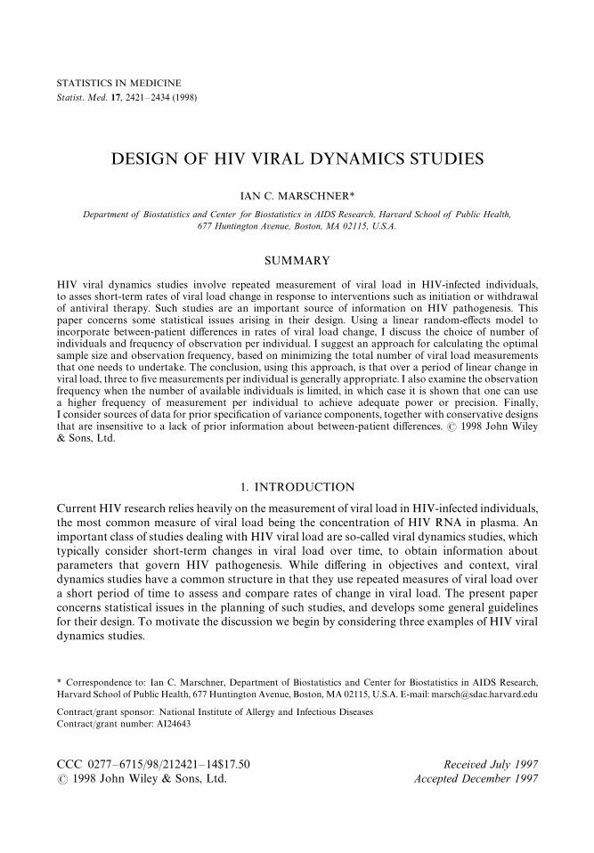
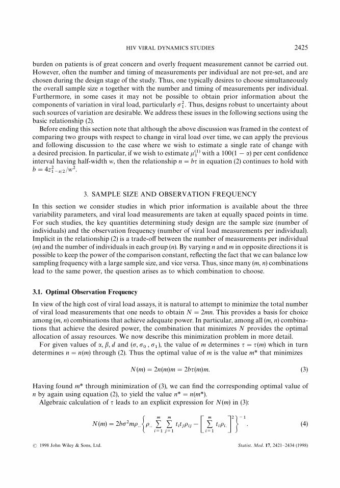
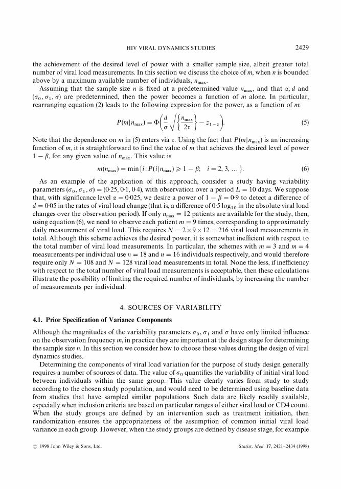
illustrates the fact that lower overall sample size may be substantially less efficient with respect toallocation of assay resources. In particular, while more frequent sampling (large m) is associatedwith a lower required sample size, it is also associated with a larger total number of viral loadmeasurements. For example, the optimal scheme having m"3 measurements per individualrequires approximately 50 per cent more individuals on study than the scheme with m"11, yetrequires only 40 per cent of the viral load measurements that the m"11 scheme would require.However, in the present context, the benefits of less frequent sampling do not extend to theextreme case of m"2 observations per individual; in this case, the total number of viral loadmeasurements is greater than the optimal scheme and indeed all other schemes with m)11.

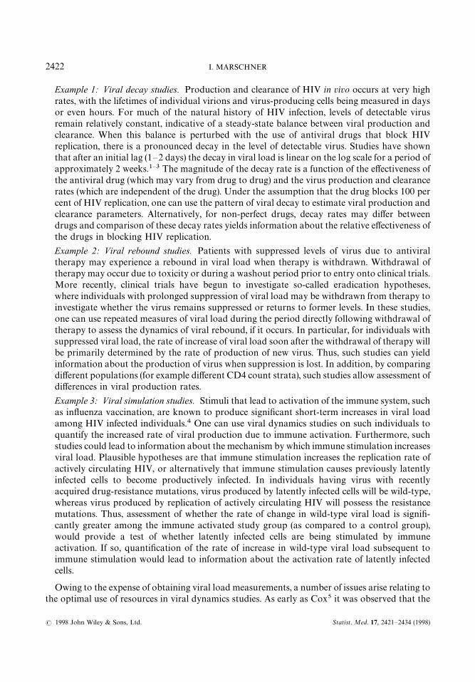
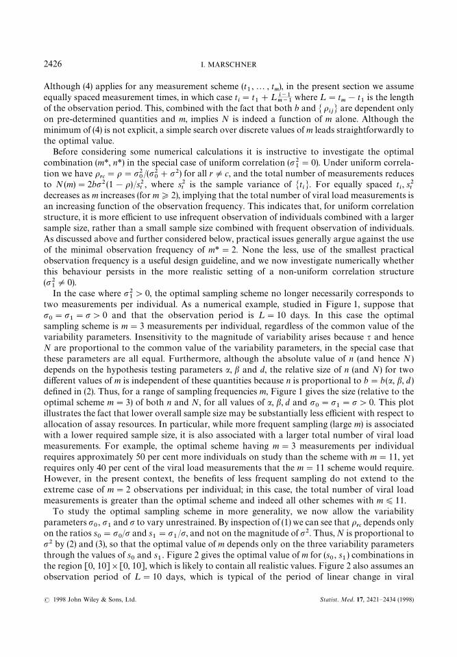
To study the optimal sampling scheme in more generality, we now allow the variabilityparameters p

0, p

1and p to vary unrestrained. By inspection of (1) we can see that o

rcdepends only

on the ratios s0"p

0/p and s

1"p

1/p, and not on the magnitude of p2. Thus, N is proportional to

p2 by (2) and (3), so that the optimal value of m depends only on the three variability parametersthrough the values of s

0and s

1. Figure 2 gives the optimal value of m for (s

0, s

1) combinations in

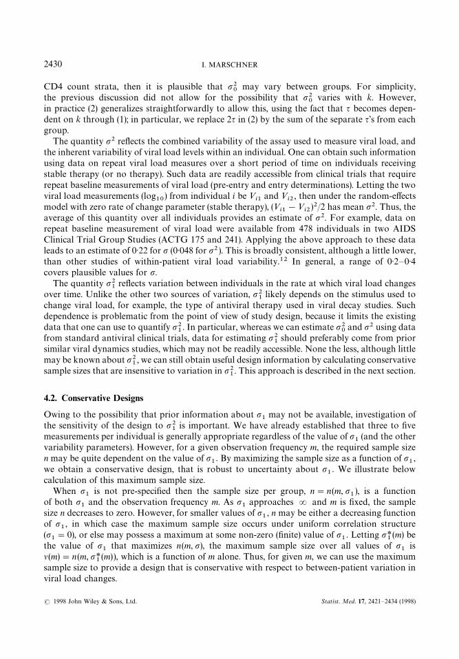
the region [0, 10]][0, 10], which is likely to contain all realistic values. Figure 2 also assumes anobservation period of ¸"10 days, which is typical of the period of linear change in viral

2426 I. MARSCHNER


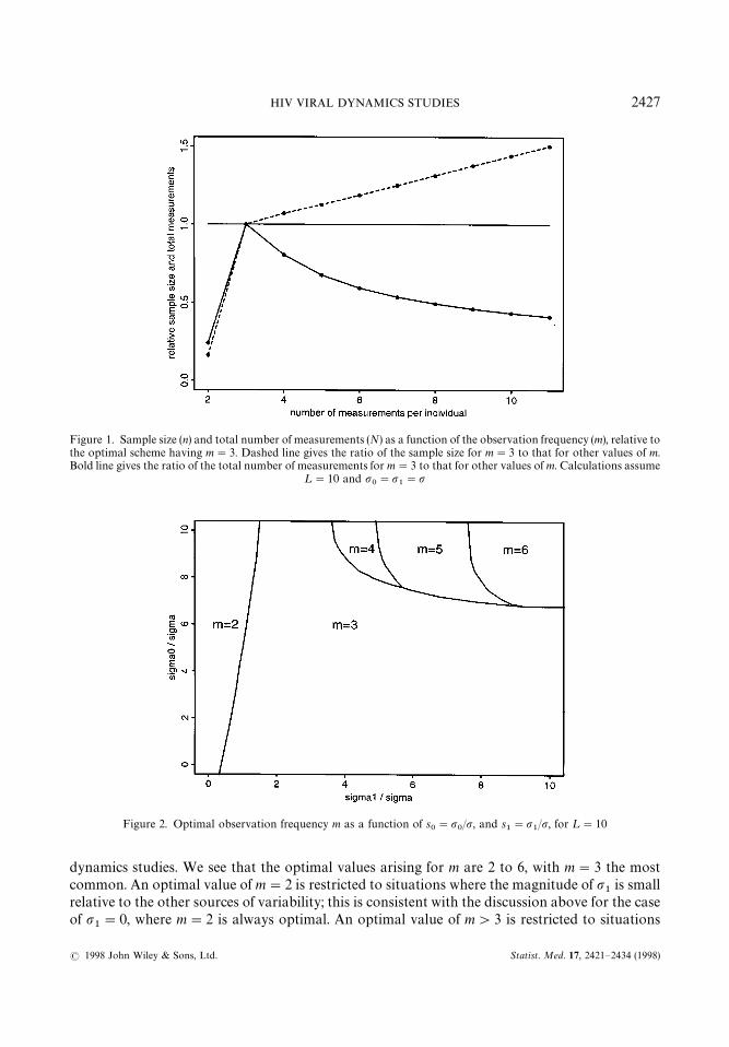
Figure 1. Sample size (n) and total number of measurements (N) as a function of the observation frequency (m), relative tothe optimal scheme having m"3. Dashed line gives the ratio of the sample size for m"3 to that for other values of m.Bold line gives the ratio of the total number of measurements for m"3 to that for other values of m. Calculations assume

¸"10 and p0"p

1"p

Figure 2. Optimal observation frequency m as a function of s0"p

0/p, and s

1"p

1/p, for ¸"10

dynamics studies. We see that the optimal values arising for m are 2 to 6, with m"3 the mostcommon. An optimal value of m"2 is restricted to situations where the magnitude of p

1is small

relative to the other sources of variability; this is consistent with the discussion above for the caseof p

1"0, where m"2 is always optimal. An optimal value of m'3 is restricted to situations



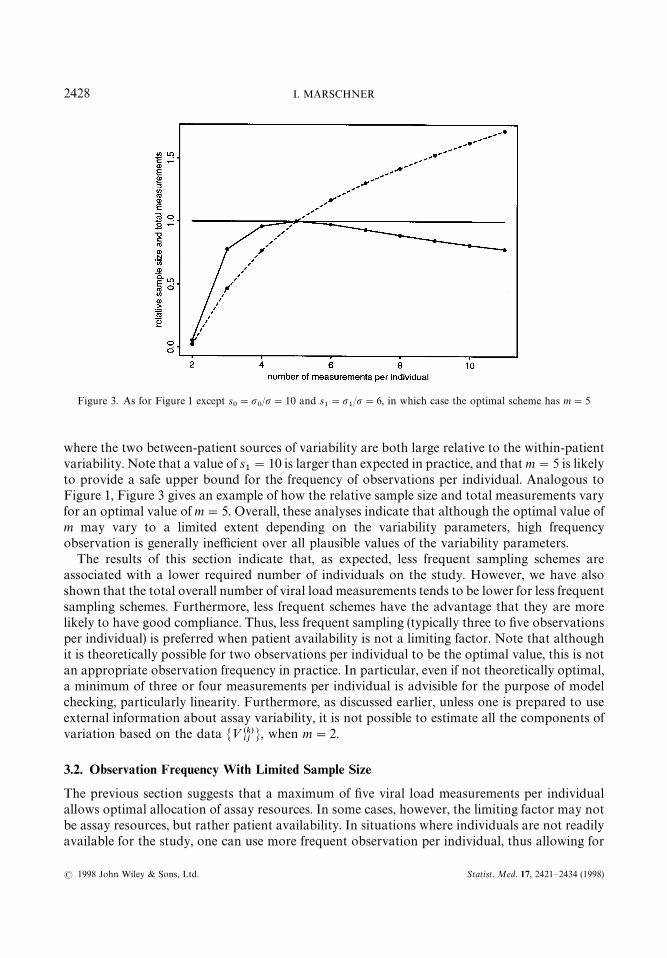
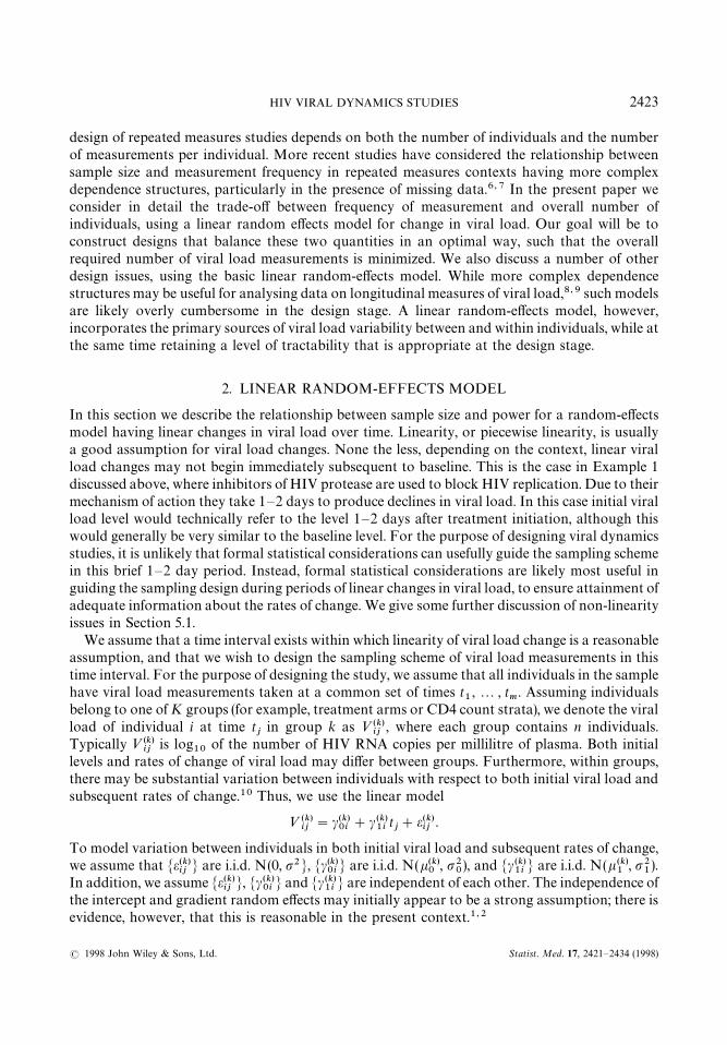
Figure 3. As for Figure 1 except s0"p

0/p"10 and s

1"p

1/p"6, in which case the optimal scheme has m"5

where the two between-patient sources of variability are both large relative to the within-patientvariability. Note that a value of s

1"10 is larger than expected in practice, and that m"5 is likely

to provide a safe upper bound for the frequency of observations per individual. Analogous toFigure 1, Figure 3 gives an example of how the relative sample size and total measurements varyfor an optimal value of m"5. Overall, these analyses indicate that although the optimal value ofm may vary to a limited extent depending on the variability parameters, high frequencyobservation is generally inefficient over all plausible values of the variability parameters.

The results of this section indicate that, as expected, less frequent sampling schemes areassociated with a lower required number of individuals on the study. However, we have alsoshown that the total overall number of viral load measurements tends to be lower for less frequentsampling schemes. Furthermore, less frequent schemes have the advantage that they are morelikely to have good compliance. Thus, less frequent sampling (typically three to five observationsper individual) is preferred when patient availability is not a limiting factor. Note that althoughit is theoretically possible for two observations per individual to be the optimal value, this is notan appropriate observation frequency in practice. In particular, even if not theoretically optimal,a minimum of three or four measurements per individual is advisible for the purpose of modelchecking, particularly linearity. Furthermore, as discussed earlier, unless one is prepared to useexternal information about assay variability, it is not possible to estimate all the components ofvariation based on the data M» (k)

ijN, when m"2.

3.2. Observation Frequency With Limited Sample Size

The previous section suggests that a maximum of five viral load measurements per individualallows optimal allocation of assay resources. In some cases, however, the limiting factor may notbe assay resources, but rather patient availability. In situations where individuals are not readilyavailable for the study, one can use more frequent observation per individual, thus allowing for

2428 I. MARSCHNER


the achievement of the desired level of power with a smaller sample size, albeit greater totalnumber of viral load measurements. In this section we discuss the choice of m, when n is boundedabove by a maximum available number of individuals, n

.!9.

Assuming that the sample size n is fixed at a predetermined value n.!9

, and that a, d and(p

0, p

1, p) are predetermined, then the power becomes a function of m alone. In particular,

rearranging equation (2) leads to the following expression for the power, as a function of m:

P(m Dn.!9

)"'Ad

pSGn.!92q H!z

1~aB. (5)

Note that the dependence on m in (5) enters via q. Using the fact that P (m Dn.!9

) is an increasingfunction of m, it is straightforward to find the value of m that achieves the desired level of power1!b, for any given value of n

.!9. This value is

m(n.!9

)"minMi :P ( i Dn.!9

)*1!b; i"2, 3,2N. (6)

As an example of the application of this approach, consider a study having variabilityparameters (p

0, p

1, p)"(0)25, 0)1, 0)4), with observation over a period ¸"10 days. We suppose

that, with significance level a"0)025, we desire a power of 1!b"0)9 to detect a difference ofd"0)05 in the rates of viral load change (that is, a difference of 0)5 log

10in the absolute viral load

changes over the observation period). If only n.!9

"12 patients are available for the study, then,using equation (6), we need to observe each patient m"9 times, corresponding to approximatelydaily measurement of viral load. This requires N"2]9]12"216 viral load measurements intotal. Although this scheme achieves the desired power, it is somewhat inefficient with respect tothe total number of viral load measurements. In particular, the schemes with m"3 and m"4measurements per individual use n"18 and n"16 individuals respectively, and would thereforerequire only N"108 and N"128 viral load measurements in total. None the less, if inefficiencywith respect to the total number of viral load measurements is acceptable, then these calculationsillustrate the possibility of limiting the required number of individuals, by increasing the numberof measurements per individual.

4. SOURCES OF VARIABILITY

4.1. Prior Specification of Variance Components

Although the magnitudes of the variability parameters p0, p

1and p have only limited influence

on the observation frequency m, in practice they are important at the design stage for determiningthe sample size n. In this section we consider how to choose these values during the design of viraldynamics studies.

Determining the components of viral load variation for the purpose of study design generallyrequires a number of sources of data. The value of p

0quantifies the variability of initial viral load

between individuals within the same group. This value clearly varies from study to studyaccording to the chosen study population, and would need to be determined using baseline datafrom studies that have sampled similar populations. Such data are likely readily available,especially when inclusion criteria are based on particular ranges of either viral load or CD4 count.When the study groups are defined by an intervention such as treatment initiation, thenrandomization ensures the appropriateness of the assumption of common initial viral loadvariance in each group. However, when the study groups are defined by disease stage, for example



CD4 count strata, then it is plausible that p20

may vary between groups. For simplicity,the previous discussion did not allow for the possibility that p2

0varies with k. However,

in practice (2) generalizes straightforwardly to allow this, using the fact that q becomes depen-dent on k through (1); in particular, we replace 2q in (2) by the sum of the separate q’s from eachgroup.

The quantity p2 reflects the combined variability of the assay used to measure viral load, andthe inherent variability of viral load levels within an individual. One can obtain such informationusing data on repeat viral load measures over a short period of time on individuals receivingstable therapy (or no therapy). Such data are readily accessible from clinical trials that requirerepeat baseline measurements of viral load (pre-entry and entry determinations). Letting the twoviral load measurements (log

10) from individual i be »

i1and »

i2, then under the random-effects

model with zero rate of change parameter (stable therapy), (»i1!»

i2)2/2 has mean p2. Thus, the

average of this quantity over all individuals provides an estimate of p2. For example, data onrepeat baseline measurement of viral load were available from 478 individuals in two AIDSClinical Trial Group Studies (ACTG 175 and 241). Applying the above approach to these dataleads to an estimate of 0)22 for p (0)048 for p2 ). This is broadly consistent, although a little lower,than other studies of within-patient viral load variability.12 In general, a range of 0)2—0)4covers plausible values for p.

The quantity p21

reflects variation between individuals in the rate at which viral load changesover time. Unlike the other two sources of variation, p2

1likely depends on the stimulus used to

change viral load, for example, the type of antiviral therapy used in viral decay studies. Suchdependence is problematic from the point of view of study design, because it limits the existingdata that one can use to quantify p2

1. In particular, whereas we can estimate p2

0and p2 using data

from standard antiviral clinical trials, data for estimating p21

should preferably come from priorsimilar viral dynamics studies, which may not be readily accessible. None the less, although littlemay be known about p2

1, we can still obtain useful design information by calculating conservative

sample sizes that are insensitive to variation in p21. This approach is described in the next section.

4.2. Conservative Designs

Owing to the possibility that prior information about p1

may not be available, investigation ofthe sensitivity of the design to p2

1is important. We have already established that three to five

measurements per individual is generally appropriate regardless of the value of p1

(and the othervariability parameters). However, for a given observation frequency m, the required sample sizen may be quite dependent on the value of p

1. By maximizing the sample size as a function of p

1,

we obtain a conservative design, that is robust to uncertainty about p1. We illustrate below

calculation of this maximum sample size.When p

1is not pre-specified then the sample size per group, n"n(m, p

1), is a function

of both p1

and the observation frequency m. As p1

approaches R and m is fixed, the samplesize n decreases to zero. However, for smaller values of p

1, n may be either a decreasing function

of p1, in which case the maximum sample size occurs under uniform correlation structure

(p1"0), or else may possess a maximum at some non-zero (finite) value of p

1. Letting p*

1(m) be

the value of p1

that maximizes n(m, p), the maximum sample size over all values of p1

isl(m)"n (m, p*

1(m)), which is a function of m alone. Thus, for given m, we can use the maximum

sample size to provide a design that is conservative with respect to between-patient variation inviral load changes.

2430 I. MARSCHNER


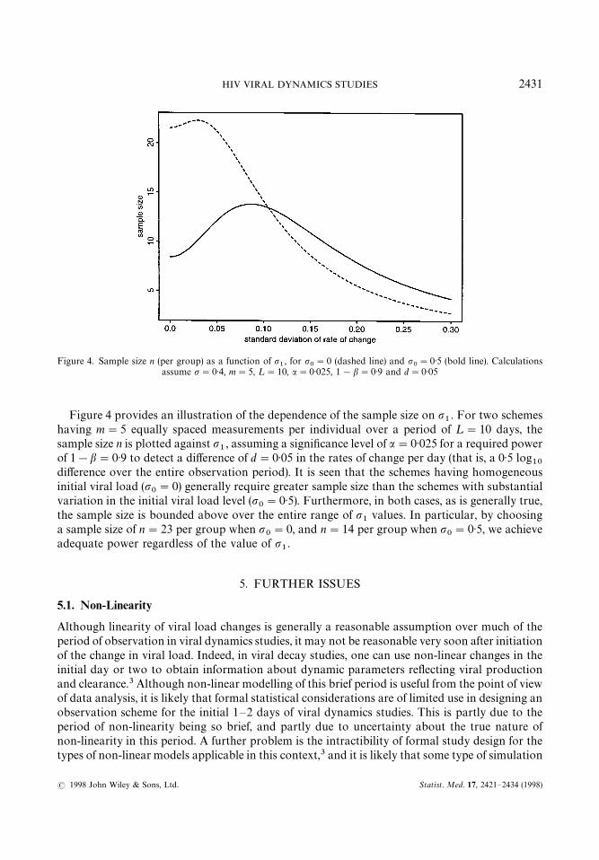
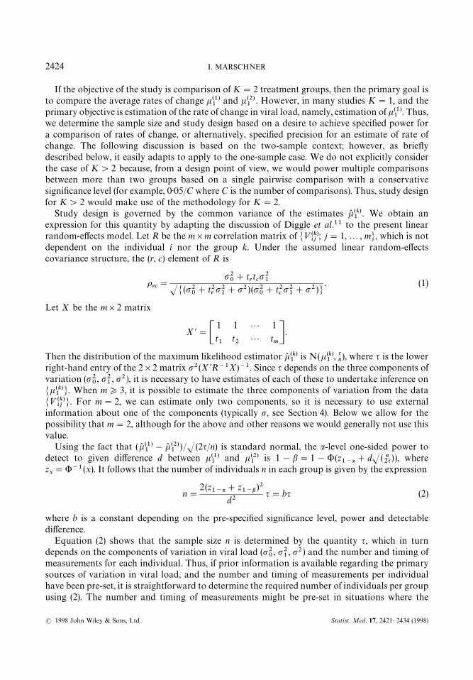
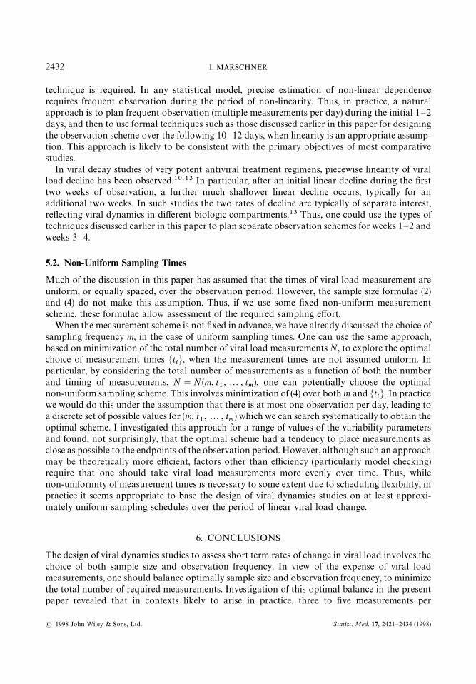
Figure 4. Sample size n (per group) as a function of p1, for p

0"0 (dashed line) and p

0"0)5 (bold line). Calculations

assume p"0)4, m"5, ¸"10, a"0)025, 1!b"0)9 and d"0)05

Figure 4 provides an illustration of the dependence of the sample size on p1. For two schemes

having m"5 equally spaced measurements per individual over a period of ¸"10 days, thesample size n is plotted against p

1, assuming a significance level of a"0)025 for a required power

of 1!b"0)9 to detect a difference of d"0)05 in the rates of change per day (that is, a 0)5 log10

difference over the entire observation period). It is seen that the schemes having homogeneousinitial viral load (p

0"0) generally require greater sample size than the schemes with substantial

variation in the initial viral load level (p0"0)5). Furthermore, in both cases, as is generally true,

the sample size is bounded above over the entire range of p1

values. In particular, by choosinga sample size of n"23 per group when p

0"0, and n"14 per group when p

0"0)5, we achieve

adequate power regardless of the value of p1.

5. FURTHER ISSUES

5.1. Non-Linearity

Although linearity of viral load changes is generally a reasonable assumption over much of theperiod of observation in viral dynamics studies, it may not be reasonable very soon after initiationof the change in viral load. Indeed, in viral decay studies, one can use non-linear changes in theinitial day or two to obtain information about dynamic parameters reflecting viral productionand clearance.3 Although non-linear modelling of this brief period is useful from the point of viewof data analysis, it is likely that formal statistical considerations are of limited use in designing anobservation scheme for the initial 1—2 days of viral dynamics studies. This is partly due to theperiod of non-linearity being so brief, and partly due to uncertainty about the true nature ofnon-linearity in this period. A further problem is the intractibility of formal study design for thetypes of non-linear models applicable in this context,3 and it is likely that some type of simulation



technique is required. In any statistical model, precise estimation of non-linear dependencerequires frequent observation during the period of non-linearity. Thus, in practice, a naturalapproach is to plan frequent observation (multiple measurements per day) during the initial 1—2days, and then to use formal techniques such as those discussed earlier in this paper for designingthe observation scheme over the following 10—12 days, when linearity is an appropriate assump-tion. This approach is likely to be consistent with the primary objectives of most comparativestudies.

In viral decay studies of very potent antiviral treatment regimens, piecewise linearity of viralload decline has been observed.10,13 In particular, after an initial linear decline during the firsttwo weeks of observation, a further much shallower linear decline occurs, typically for anadditional two weeks. In such studies the two rates of decline are typically of separate interest,reflecting viral dynamics in different biologic compartments.13 Thus, one could use the types oftechniques discussed earlier in this paper to plan separate observation schemes for weeks 1—2 andweeks 3—4.

5.2. Non-Uniform Sampling Times

Much of the discussion in this paper has assumed that the times of viral load measurement areuniform, or equally spaced, over the observation period. However, the sample size formulae (2)and (4) do not make this assumption. Thus, if we use some fixed non-uniform measurementscheme, these formulae allow assessment of the required sampling effort.

When the measurement scheme is not fixed in advance, we have already discussed the choice ofsampling frequency m, in the case of uniform sampling times. One can use the same approach,based on minimization of the total number of viral load measurements N, to explore the optimalchoice of measurement times Mt

iN, when the measurement times are not assumed uniform. In

particular, by considering the total number of measurements as a function of both the numberand timing of measurements, N"N(m, t

1,2, t

m), one can potentially choose the optimal

non-uniform sampling scheme. This involves minimization of (4) over both m and MtiN. In practice

we would do this under the assumption that there is at most one observation per day, leading toa discrete set of possible values for (m, t

1,2, t

m) which we can search systematically to obtain the

optimal scheme. I investigated this approach for a range of values of the variability parametersand found, not surprisingly, that the optimal scheme had a tendency to place measurements asclose as possible to the endpoints of the observation period. However, although such an approachmay be theoretically more efficient, factors other than efficiency (particularly model checking)require that one should take viral load measurements more evenly over time. Thus, whilenon-uniformity of measurement times is necessary to some extent due to scheduling flexibility, inpractice it seems appropriate to base the design of viral dynamics studies on at least approxi-mately uniform sampling schedules over the period of linear viral load change.

6. CONCLUSIONS

The design of viral dynamics studies to assess short term rates of change in viral load involves thechoice of both sample size and observation frequency. In view of the expense of viral loadmeasurements, one should balance optimally sample size and observation frequency, to minimizethe total number of required measurements. Investigation of this optimal balance in the presentpaper revealed that in contexts likely to arise in practice, three to five measurements per

2432 I. MARSCHNER


individual is appropriate, taken at approximately equally spaced points in time over the first twoweeks of observation. If desired, one may augment such sampling by higher frequency samplingvery soon after viral decay or rebound begins, in order to capture non-linear behaviour duringdays one and two. In viral decay studies involving suppression over a period longer than twoweeks, an additional three to five measurements per individual are required to assess rates ofdecay during weeks three and four, due to the separate dynamics during this period.

Having determined the frequency of observation per individual, one can determine the requirednumber of individuals on study to achieve adequate information for estimation and comparisonof rates of viral load change. When the number of available individuals is limited, one can usegreater frequency of viral load measurement to reduce the required number of individuals.However, it is important to balance the advantages of having a smaller sample size against thefact that schemes with high observation frequency pose greater difficulties for compliance, andgenerally require a greater total number of viral load measurements than do low frequencyschemes.

As in any design context, prior information about sources of variability is important in thedesign of viral dynamics studies. There are three primary components of variation in viral loadthat affect the design of viral dynamics studies: (i) variation between patients in the baseline viralload level; (ii) variation between patients in the rate of change of viral load; and (iii) within-patientvariation in viral load due to biological and assay variation. Since little information may beavailable about variance component (ii), one can calculate conservative sample sizes thatmaximize over component (ii) using knowledge of the other two variance components. This canprovide information about the potential sensitivity of the design to between-patient variation inviral load rates of change. In addition to the components of viral load variability, the studydesign also depends on any correlation that exists between the initial viral load and thesubsequent rate of viral load change. We did not allow explicitly for this correlation here,and available data suggest that this is an appropriate assumption. None the less, the presentmethodology extends straightforwardly to accommodate such correlation. In particular,when we assume that the patient-specific intercept and gradient terms have non-zero correla-tion /, the correlation structure (1) generalizes straightforwardly; thus, the basic relationship(2), and all the subsequent methodology, is unchanged except that dependence on / entersthrough (1). In practice, however, it is most likely that / is positive (if it is not zero), in which casethe sample sizes corresponding to /"0 are conservative. Thus, the assumption that /"0, asused in this paper, is generally appropriate given that accurate information on / is unlikelyavailable.

In considering the design of viral dynamics studies it is natural to make a number of simplifyingassumptions, both for tractability and because more complex models require information notavailable prior to the study. In the present context such simplifying assumptions include: constantvariance across the entire range of viral load measurements; a dependence structure for repeatedviral load measurements corresponding to a linear random-effects model; and normalityof viral load measurements (on the log

10scale). In practice it may be useful to relax these

and other assumptions in analysing data on viral load. None the less, the model usedhere incorporates important sources of viral load variability between and within patients,while retaining an appropriate level of simplicity for study design. Thus, despite the potential formore complex models at the analysis stage, the discussion presented here provides generalmethods and guidelines that should prove useful at the design stage of HIV viral dynamicsstudies.



ACKNOWLEDGEMENTS

My thanks to members of the AIDS Clinical Trials Group Viral Dynamics Focus Group forhelpful discussions. This research was supported by grant AI24643 from the National Institute ofAllergy and Infectious Diseases.

REFERENCES

1. Ho, D. D., Neumann, A. U., Perelson, A. S., Chen, W., Leonard, J. M. and Markowitz, M. ‘Rapidturnover of plasma virions and CD4 lymphocytes in HIV-1 infection’, Nature, 373, 123—126 (1995).

2. Wei, X., Ghosh, S. K., Taylor, M. E., Johnson, V. A., Emini, E. A., Deutsch, P., Lifson, J. D., Bonhoeffer,S., Nowak, M. A., Hahn, B. H., Saag, M. S. and Shaw, G. M. ‘Viral dynamics in human immunodefi-ciency virus type 1 infection’, Nature, 373, 117—122 (1995).

3. Perelson, A. S., Neumann, A. U., Markowitz, M., Leonard, J. M. and Ho, D. D. ‘HIV-1 dynamics in vivo:virion clearance rate, infected cell life-span, and viral generation time’, Science, 271, 1582—1586 (1996).

4. Ho, D. D. ‘HIV-1 viremia and influenza’, ¸ancet, 339, 1549 (1992).5. Cox, D. R. Planning of Experiments, Wiley, Toronto, 1958.6. Wu, M. C. ‘Sample size for comparison of changes in the presence of right censoring caused by death,

withdrawal, and staggered entry’, Controlled Clinical ¹rials, 9, 32—46 (1988).7. Dawson, J. D. and Lagakos, S. W. ‘Size and Power of two-sample tests of repeated measures data’,

Biometrics, 49, 1022—1032 (1993).8. Taylor, J. M. G., Cumberland, W. G. and Sy, J. P. ‘A stochastic model for the analysis of longitudinal

AIDS data’, Journal of the American Statistical Association, 89, 727—736 (1994).9. La Valley, M. P. and DeGruttola, V. ‘Models for empirical Bayes estimators of longitudinal CD4

counts’, Statistics in Medicine, 15, 2289—2306 (1995).10. Wu, H., Kuritzkes, D. R., St. Clair, M., Kessler, H., Connick, E., Landay, A., Heath-Chiozzi, M.,

Rousseau, F., Fox, L., Spritzler, J., Leonard, J. M., McClernon, D. R. and Lederman, M. M. ‘Interpatientvariation of viral dynamics in HIV-1 infection: Modelling results of AIDS Clinical Trials GroupProtocol 315’, The International Workshop on HIV Drug Resistance, Treatment Strategies andEradication, Antiviral ¹herapy, Abstract 99, 66—67 (1997).

11. Diggle, P. J., Liang, K. Y. and Zeger, S. L. Analysis of ¸ongitudinal Data, Clarendon Press, Oxford, 1994.12. Paxton, W. B. Coombs, R. W., McElrath, M. J., Keefer, M. C., Hughes, J., Sinangil, F., Chernoff, D.,

Demeter, L., Williams, B. and Corey, L. ‘Longitudinal analysis of quantitative virologic measures inhuman immunodeficiency virus-infected subjects with *400 CD4 lymphocytes: implications for ap-plying measurements to individual patients’, Journal of Infectious Diseases, 175, 247—254 (1997).

13. Perelson, A. S., Essunger, P., Cao, Y., Vesanen, M., Hurley, A., Saksela, K., Markowitz, M. and Ho, D.D. ‘Decay characteristics of HIV-1-infected compartments during combination therapy’, Nature, 387,188 (1997).

2434 I. MARSCHNER


design of hiv viral dynamics studies

Documents