design of experiments for engineers and scientists
TRANSCRIPT

Design of Experiments for Engineers and Scientists

Design of Experiments for Engineers and ScientistsSecond Edition
Jiju AntonySchool of Management and Languages, Heriot-Watt University, Edinburgh, Scotland, UK
AMSTERDAM • BOSTON • HEIDELBERG • LONDON • NEW YORK • OXFORD PARIS • SAN DIEGO • SAN FRANCISCO • SINGAPORE • SYDNEY • TOKYO

Elsevier32 Jamestown Road, London NW1 7BY225 Wyman Street, Waltham, MA 02451, USA
First edition 2003Second edition 2014
Copyright © 2014, 2003 Jiju Antony. Published by Elsevier Ltd. All rights reserved.
No part of this publication may be reproduced or transmitted in any form or by any means, electronic or mechanical, including photocopying, recording, or any information storage and retrieval system, without permission in writing from the publisher. Details on how to seek permission, further information about the Publisher’s permissions policies and our arrangement with organizations such as the Copyright Clearance Center and the Copyright Licensing Agency, can be found at our website: www.elsevier.com/permissions.
This book and the individual contributions contained in it are protected under copyright by the Publisher (other than as may be noted herein).
NoticesKnowledge and best practice in this field are constantly changing. As new research and experience broaden our understanding, changes in research methods, professional practices, or medical treatment may become necessary.
Practitioners and researchers must always rely on their own experience and knowledge in evaluating and using any information, methods, compounds, or experiments described herein.
In using such information or methods they should be mindful of their own safety and the safety of others, including parties for whom they have a professional responsibility.
To the fullest extent of the law, neither the Publisher nor the authors, contributors, or editors, assume any liability for any injury and/or damage to persons or property as a matter of products liability, negligence or otherwise, or from any use or operation of any methods, products, instructions, or ideas contained in the material herein.
British Library Cataloguing-in-Publication DataA catalogue record for this book is available from the British Library
Library of Congress Cataloging-in-Publication DataA catalog record for this book is available from the Library of Congress
ISBN: 978-0-08-099417-8
For information on all Elsevier publications visit our website at store.elsevier.com
This book has been manufactured using Print On Demand technology. Each copy is produced to order and is limited to black ink. The online version of this book will show color figures where appropriate.

Preface
Design of Experiments (DOE) is a powerful technique used for both exploring new processes and gaining increased knowledge of existing processes, followed by opti-mising these processes for achieving world-class performance. My involvement in promoting and training in the use of DOE dates back to the mid-1990s. There are plenty of books available in the market today on this subject written by classic stat-isticians, although the majority of them are better suited to other statisticians than to run-of-the-mill industrial engineers and business managers with limited mathemati-cal and statistical skills.
DOE never has been a favourite technique for many of today’s engineers and managers in organisations due to the number crunching involved and the statistical jargon incorporated into the teaching mode by many statisticians. This book is tar-geted to people who have either been intimidated by their attempts to learn about DOE or who have never appreciated the true potential of DOE for achieving break-through improvements in product quality and process efficiency.
This book gives a solid introduction to the technique through a myriad of practi-cal examples and case studies. The second edition of the book has incorporated two new chapters and both cover the latest developments on the topic of DOE. Readers of this book will develop a sound understanding of the theory of DOE and practical aspects of how to design, analyse and interpret the results of a designed experiment. Throughout this book, the emphasis is on the simple but powerful graphical tools available for data analysis and interpretation. All of the graphs and figures in this book were created using Minitab version 15.0 for Windows.
I sincerely hope that practising industrial engineers and managers as well as researchers in academic world will find this book useful in learning how to apply DOE in their own work environment. The book will also be a useful resource for people involved in Six Sigma training and projects related to design optimisation and process performance improvements. In fact, I have personally observed that the num-ber of applications of DOE in non-manufacturing sectors has increased significantly because of the methodology taught to Six Sigma professionals such as Six Sigma Green Belts and Black Belts.
The second edition has a chapter dedicated to DOE for non-manufacturing pro-cesses. As a mechanical engineer, I was not convinced about the application of DOE in the context of the service industry and public sector organisations including Higher Education. I have included a simple case study showing the power of DOE in a university setting. I firmly believe that DOE can be applied to any industrial set-ting, although there will be more challenges and barriers in the non-manufacturing sector compared to traditional manufacturing companies.

Prefacex
I hope that this book inspires readers to get into the habit of applying DOE for problem-solving and process troubleshooting. I strongly recommend that readers of this book continue on a more advanced reference to learn about topics which are not covered here. I am indebted to many contributors and gurus for the development of various experimental design techniques, especially Sir Ronald Fisher, Plackett and Burman, Professor George Box, Professor Douglas Montgomery, Dr Genichi Taguchi and Dr Dorian Shainin.

Acknowledgements
This book was conceived further to my publication of an article entitled ‘Teaching Experimental Design Techniques to Engineers and Managers’ in the International Journal of Engineering Education. I am deeply indebted to a number of people who, in essence, have made this book what it is today. First, and foremost, I would like to thank a number of colleagues in both the academic and industrial worlds, as well as the research scholars I have supervised over the years, for their constant encourage-ment in writing up the second edition of the book. I am also indebted to the quality and production managers of the companies that I have been privileged to work with and gather data. I would also like to take this opportunity to thank my doctoral and other postgraduate students both on campus and off campus.
I would like to express my deepest appreciation to Hayley Grey and Cari Owen for their incessant support and forbearance during the course of this project. Finally, I express my sincere thanks to my wife, Frenie, and daughter, Evelyn, for their encour-agement and patience as the book stole countless hours away from family activities.

Design of Experiments for Engineers and Scientists. DOI: Copyright © 2014 Jiju Antony. Published by Elsevier Ltd. All rights reserved.
http://dx.doi.org/10.1016/B978-0-08-099417-8.00001-8
Introduction to Industrial Experimentation
1
1.1 Introduction
Experiments are performed today in many manufacturing organisations to increase our understanding and knowledge of various manufacturing processes. Experiments in manufacturing companies are often conducted in a series of trials or tests which pro-duce quantifiable outcomes. For continuous improvement in product/process quality, it is fundamental to understand the process behaviour; the amount of variability and its impact on processes. In an engineering environment, experiments are often conducted to explore, estimate or confirm. Exploration refers to understanding the data from the process. Estimation refers to determining the effects of process variables or factors on the output performance characteristic. Confirmation implies verifying the predicted results obtained from the experiment.
In manufacturing processes, it is often of primary interest to explore the relation-ships between the key input process variables (or factors) and the output performance characteristics (or quality characteristics). For example, in a metal cutting operation, cutting speed, feed rate, type of coolant, depth of cut, etc. can be treated as input vari-ables and the surface finish of the finished part can be considered as an output per-formance characteristic. In service processes, it is often more difficult to understand what is to be measured; moreover, the process variability in the service context may be attributed to human factors, which are difficult to control. Furthermore, the delivery of service quality is heavily dependent on the situational influences of the person who provides the service.
One of the common approaches employed by many engineers today in manufactur-ing companies is One-Variable-At-a-Time (OVAT), where we vary one variable at a time and keep all other variables in the experiment fixed. This approach depends upon guesswork, luck, experience and intuition for its success. Moreover, this type of experi-mentation requires large quantities of resources to obtain a limited amount of infor-mation about the process. OVAT experiments often are unreliable, inefficient and time consuming and may yield false optimum conditions for the process.
Statistical thinking and statistical methods play an important role in planning, con-ducting, analysing and interpreting the data from engineering experiments. Statistical thinking tells us how to deal with variability, and how to collect and use data so that effective decisions can be made about the processes or systems we deal with every day. When several variables influence a certain characteristic of a product, the best strategy is then to design an experiment so that valid, reliable and sound conclusions can be drawn effectively, efficiently and economically. In a designed experiment we often make deliberate changes in the input variables (or factors) and then determine how the output

Design of Experiments for Engineers and Scientists2
functional performance varies accordingly. It is important to note that not all variables affect the performance in the same manner. Some may have strong influences on the out-put performance, some may have medium influences and some may have no influence at all. Therefore the objective of a carefully planned designed experiment is to under-stand which set of variables in a process affect the performance most and then determine the best levels for these variables to obtain satisfactory output functional performance in products. Moreover, we can also set the levels of unimportant variables to their most eco-nomic settings. This would have an immense impact on financial savings to a company’s bottom line (Clements, 1995).
Design of Experiments (DOE) was developed in the early 1920s by Sir Ronald Fisher at the Rothamsted Agricultural Field Research Station in London, England. His initial experiments were concerned with determining the effect of various fertilis-ers on different plots of land. The final condition of the crop was dependent not only on the fertiliser but also on a number of other factors (such as underlying soil con-dition, moisture content of the soil, etc.) of each of the respective plots. Fisher used DOE that could differentiate the effect of fertiliser from the effects of other factors. Since then, DOE has been widely accepted and applied in biological and agricultural fields. A number of successful applications of DOE have been reported by many US and European manufacturers over the last 15 years or so. The potential applications of DOE in manufacturing processes include (Montgomery et al., 1998):
● improved process yield and stability● improved profits and return on investment● improved process capability● reduced process variability and hence better product performance consistency● reduced manufacturing costs● reduced process design and development time● heightened engineers’ morale with success in solving chronic problems● increased understanding of the relationship between key process inputs and output(s)● increased business profitability by reducing scrap rate, defect rate, rework, retest, etc.
Similarly, the potential applications of DOE in service processes include:
● identifying the key service process or system variables which influence the process or sys-tem performance
● identifying the service design parameters which influence the service quality characteris-tics in the eyes of customers
● minimising the time to respond to customer complaints● minimising errors on service orders● reducing the service delivery time to customers (e.g. banks, restaurants)● reducing the turn-around time in producing reports to patients in a healthcare environment,
and so on.
Industrial experiments involve a sequence of activities:
1. Hypothesis – an assumption that motivates the experiment2. Experiment – a series of tests conducted to investigate the hypothesis3. Analysis – understanding the nature of data and performing statistical analysis of the
collected data from the experiment

Introduction to Industrial Experimentation 3
4. Interpretation – understanding the results of the experimental analysis5. Conclusion – stating whether or not the original set hypothesis is true or false. Very often
more experiments are to be performed to test the hypothesis and sometimes we establish a new hypothesis that requires more experiments.
Consider a welding process where the primary concern of interest to engineers is the strength of the weld and the variation in the weld strength values. Through sci-entific experimentation, we can determine what factors mostly affect the mean weld strength and the variation in weld strength. Through experimentation, one can also pre-dict the weld strength under various conditions of key input welding machine param-eters or factors (e.g. weld speed, voltage, welding time, weld position, etc.).
For the successful application of an industrial designed experiment, we generally require the following skills:
● Planning skills: Understanding the significance of experimentation for a particular prob-lem, time and experimental budget required for the experiment, how many people are involved with the experimentation, establishing who is doing what, etc.
● Statistical skills: The statistical analysis of data obtained from the experiment, assignment of factors and interactions to various columns of the design matrix (or experimental lay-out), interpretation of results from the experiment for making sound and valid decisions for improvement, etc.
● Teamwork skills: Understanding the objectives of the experiment and having a shared understanding of the experimental goals to be achieved, better communication among peo-ple with different skills and learning from one another, brainstorming of factors for the experiment by team members, etc.
● Engineering skills: Determination of the number of levels of each factor and the range at which each factor can be varied, determination of what to measure within the experiment, determination of the capability of the measurement system in place, determination of what factors can be controlled and what cannot be controlled for the experiment, etc.
1.2 Some Fundamental and Practical Issues in Industrial Experimentation
An engineer is interested in measuring the yield of a chemical process, which is influ-enced by two key process variables (or control factors). The engineer decides to per-form an experiment to study the effects of these two variables on the process yield. The engineer uses an OVAT approach to experimentation. The first step is to keep the tem-perature constant (T1) and vary the pressure from P1 to P2. The experiment is repeated twice and the results are illustrated in Table 1.1. The engineer conducts four experi-mental trials.
The next step is to keep the pressure constant (P1) and vary the temperature from T1 to T2. The results of the experiment are given in Table 1.2.
The engineer has calculated the average yield values for only three combinations of temperature and pressure: (T1, P1), (T1, P2) and (T2, P1). The engineer concludes from the experiment that the maximum yield of the process can be attained by corresponding to (T1, P2). The question then arises as to what should be the average yield corresponding to

Design of Experiments for Engineers and Scientists4
the combination (T2, P2)? The engineer was unable to study this combination as well as the interaction between temperature and pressure. Interaction between two factors exists when the effect of one factor on the response or output is different at different levels of the other factor. The difference in the average yield between the trials one and two pro-vides an estimate of the effect of pressure. Similarly, the difference in the average yield between trials three and four provide an estimate of the effect of temperature. An effect of a factor is the change in the average response due to a change in the levels of a factor. The effect of pressure was estimated to be 8% (i.e. 64−56) when temperature was kept constant at ‘T1’. There is no guarantee whatsoever that the effect of pressure will be the same when the conditions of temperature change. Similarly the effect of temperature was estimated to be 5% (i.e. 61−56) when pressure was kept constant at ‘P1’. It is reasonable to say that we do not get the same effect of temperature when the conditions of pres-sure change. Therefore the OVAT approach to experimentation can be misleading and may lead to unsatisfactory experimental conclusions in real-life situations. Moreover, the success of the OVAT approach to experimentation relies on guesswork, luck, experience and intuition (Antony, 1997). This type of experimentation is inefficient in that it requires large resources to obtain a limited amount of information about the process. In order to obtain a reliable and predictable estimate of factor effects, it is important that we vary the factors simultaneously at their respective levels. In the above example, the engineer should have varied the levels of temperature and pressure simultaneously to obtain reli-able estimates of the effects of temperature and pressure. The focus of this book is to explain the rationale behind such carefully planned and well-designed experiments.
A study carried out at the University of Navarra, Spain, has shown that 80% of the companies (sample size of 128) in the Basque Country conduct experimentation using the OVAT strategy. Moreover, it was found that only 20% of companies carry out experimentation with a pre-established statistical methodology (Tanco et al., 2008). The findings of Tanco et al. have also revealed that the size of the industry plays a large part in DOE awareness; only 22% of small companies are familiar with DOE, as compared with 43% of medium-sized companies and 76% of large companies (sam-ple size of 133).
Table 1.1 The Effects of Varying Pressure on Process Yield
Trial Temperature Pressure Yield Average Yield (%)
1 T1 P1 55, 57 562 T1 P2 63, 65 64
Table 1.2 The Effects of Varying Temperature on Process Yield
Trial Temperature Pressure Yield Average Yield (%)
3 T1 P1 55, 57 564 T2 P1 60, 62 61

Introduction to Industrial Experimentation 5
1.3 Statistical Thinking and its Role Within DOE
One of the success factors for the effective deployment of DOE in any organisation is the uncompromising commitment of the senior management team and visionary leadership. However, it is not essential that the senior managers have a good technical knowledge of the working mechanisms of DOE, although the author argues that they should have a good understanding of the term ‘statistical thinking’. Statistical thinking is a philosophy of learning and action based on the following three fundamental princi-ples (Snee, 1990):
1. All work occurs in a system of interconnected processes.2. Variation exists in all processes.3. Understanding and reducing variation are the key to success.
The importance of statistical thinking derives from the fundamental principle of quality put forth by Deming: ‘Reduce variation and you improve quality’. Customers of today and tomorrow value products and services that have consistent performance, which can be achieved by systematically eliminating variation in business processes (ASQ, 1996). However, our managers lack statistical thinking and some of the possible reasons for this are as follows:
● A shift in the organisation’s priorities – Global competition has forced managers to rethink how organisations are run and to search for better ways to manage. Problem solving in manufacturing and R&D, while important, is not seen as particularly relevant to the needs of management.
● Managers view statistics as a tool for ‘fire fighting’ actions – One of the most difficult challenges for every manager is to figure out how to use statistical thinking effectively to help them make effective decisions. When a problem arises in the business, managers want to fix it as soon as possible so that they can deal with their day-to-day activities. However, what they do not realise is that the majority of problems are in systems or processes that can only be tackled with the support of senior management team. The result is that man-agement spends too much time ‘fire fighting’, solving the same problem again and again because the system was not changed. These scenarios are as follows:● A change in the mindset of people in the enterprise – Philosopher George Bernard Shaw
once said, ‘If you cannot change your mind, you cannot change anything’. It is clear that managers, quality professionals and statisticians all have new roles that require new skills. Change implies discontinuity and the destruction of familiar structures and rela-tionships. Change can be resisted because it involves confrontation of the unknown and loss of the familiar (Huczynski and Buchanan, 2001).
● Fear of statistics by managers – Even if managers were taught statistics at university, it was usually focused on complex maths and formulas rather than the application of statistical tools for problem solving and an effective decision-making process. Usually managers have their first experience with statistical thinking in a workshop inside the company, applying some tools with the guidance of an expert. Although this is the best learning method for understanding and experiencing statistical thinking, managers may still struggle to apply the principles to a different problem. This fundamental problem can be tackled by teaching usable and practical statistical techniques through real case studies at the university level.

Design of Experiments for Engineers and Scientists6
Exercises
1. Why do we need to perform experiments in organisations?2. What are the limitations of the OVAT approach to experimentation?3. What types of skills are required to make an experiment successful in organisations?4. Why is statistical thinking highly desirable for senior managers and leaders of
organisations?
References
American Society of Quality, 1996. Glossary and Tables for Statistical Quality Control. Statistics Division, Quality Press, Milwaukee, WI.
Antony, J., 1997. A Strategic Methodology to the Use of Advanced Statistical Quality Improvement Techniques (PhD thesis). University of Portsmouth, UK.
Clements, R.B., 1995. The Experimenter’s Companion. ASQC Quality Press, Milwaukee, WI.Huczynski, A., Buchanan, D., 2001. Organisational Behaviour: An Introductory Text, fourth
ed. Prentice-Hall, New Jersey, USA.Montgomery, D.C., Runger, G.C., Hubele, N.F., 1998. Engineering Statistics. John Wiley &
Sons, New York, NY.Snee, R., 1990. Statistical thinking and its contribution to total quality. Am. Stat. 44 (2),
116–121.Tanco, M, et al., 2008. Is design of experiments really used? A survey of Basque industries. J.
Eng. Des. 19 (5), 447–460.

Design of Experiments for Engineers and Scientists. DOI: Copyright © 2014 Jiju Antony. Published by Elsevier Ltd. All rights reserved.
http://dx.doi.org/10.1016/B978-0-08-099417-8.00002-X
Fundamentals of Design of Experiments
2
2.1 Introduction
In order to properly understand a designed experiment, it is essential to have a good understanding of the process. A process is the transformation of inputs into outputs. In the context of manufacturing, inputs are factors or process variables such as people, materials, methods, environment, machines, procedures, etc. and outputs can be perfor-mance characteristics or quality characteristics of a product. Sometimes, an output can also be referred to as response. In the context of Six Sigma, this is often referred to as critical-to-quality characteristics.
In performing a designed experiment, we will intentionally make changes to the input process or machine variables (or factors) in order to observe correspond-ing changes in the process output. If we are dealing with a new product development process, we will make changes to the design parameters in order to make the design performance insensitive to all sources of variation (Montgomery, 2001). The informa-tion gained from properly planned, executed and analysed experiments can be used to improve functional performance of products, to reduce the scrap rate or rework rate, to reduce product development cycle time, to reduce excessive variability in production processes, to improve throughput yield of processes, to improve the capability of pro-cesses, etc. Let us suppose that an experimenter wishes to study the influence of five variables or factors on an injection moulding process. Figure 2.1 illustrates an example of an injection moulding process with possible inputs and outputs. The typical outputs of an injection moulding process can be length, thickness, width etc. of an injection moulded part. However, these outputs can be dependant on a number of input variables such as mould temperature, injection pressure, injection speed, etc. which could have an impact on the above mentioned outputs. The purpose of a designed experiment is to understand the relationship between a set of input variables and an output or outputs.
Now consider a wave soldering process where the output is the number of sol-der defects. The possible input variables which might influence the number of solder defects are type of flux, type of solder, flux coating depth, solder temperature, etc. More recently, DOE has been accepted as a powerful technique in the service industry and there have been some major achievements. For instance, a credit card company in the US has used DOE to increase the response rate to their mailings. They have changed the colour, envelope size, character type and text within the experiment.
In real-life situations, some of the process variables or factors can be controlled fairly easily and some of them are difficult or expensive to control during normal production or standard conditions. Figure 2.2 illustrates a general model of a process or system.

Design of Experiments for Engineers and Scientists8
In Figure 2.2, output(s) are performance characteristics which are measured to assess process/product performance. Controllable variables (represented by X’s) can be varied easily during an experiment and such variables have a key role to play in the process characterisation. Uncontrollable variables (represented by Z’s) are dif-ficult to control during an experiment. These variables or factors are responsible for variability in product performance or product performance inconsistency. It is impor-tant to determine the optimal settings of X’s in order to minimise the effects of Z’s. This is the fundamental strategy of robust design (Roy, 2001).
2.2 Basic Principles of DOE
DOE refers to the process of planning, designing and analysing the experiment so that valid and objective conclusions can be drawn effectively and efficiently. In order
Mould temperature Length of moulded part
Gate size
Holding pressure Width of moulded part
Screw speed
Thickness of moulded partPercent regrind
Type of raw material
Manufacturing process ofinjection
moulded parts
Figure 2.1 Illustration of an injection moulding process.
Controllable variables (factors)
(X1) (X2) … (Xn)
Input (s) Output (s)
(Y)
(Z1) (Z2) … (Zn)
Uncontrollable variables (factors)
Process/system
Figure 2.2 General model of a process/system.

Fundamentals of Design of Experiments 9
to draw statistically sound conclusions from the experiment, it is necessary to inte-grate simple and powerful statistical methods into the experimental design methodol-ogy (Vecchio, 1997). The success of any industrially designed experiment depends on sound planning, appropriate choice of design, statistical analysis of data and teamwork skills.
In the context of DOE in manufacturing, one may come across two types of pro-cess variables or factors: qualitative and quantitative. For quantitative factors, one must decide on the range of settings and how they are to be measured and controlled during the experiment. For example, in the above injection moulding process, screw speed, mould temperature, etc. are examples of quantitative factors. Qualitative factors are discrete in nature. Type of raw material, type of catalyst, type of supplier, etc. are examples of qualitative factors. A factor may take different levels, depending on the nature of the factor – quantitative or qualitative. A qualitative factor generally requires more levels when compared to a quantitative factor. Here the term ‘level’ refers to a specified value or setting of the factor being examined in the experiment. For instance, if the experiment is to be performed using three different types of raw materials, then we can say that the factor – the type of raw material – has three levels.
In the DOE terminology, a trial or run is a certain combination of factor levels whose effect on the output (or performance characteristic) is of interest.
The three principles of experimental design, namely randomisation, replication and blocking, can be utilised in industrial experiments to improve the efficiency of experi-mentation (Antony, 1997). These principles of experimental design are applied to reduce or even remove experimental bias. It is important to note that large experimen-tal bias could result in wrong optimal settings or, in some cases, could mask the effect of the really significant factors. Thus an opportunity for gaining process understanding is lost, and a primary element for process improvement is overlooked.
2.2.1 Randomisation
We all live in a non-stationary world, a world in which noise factors (or external dis-turbances) will never stay still. For instance, the manufacture of a metal part is an operation involving people, machines, measurement, environment, etc. The parts of the machine are not fixed entities; they wear out over a period of time and their accuracy is not constant over time. The attitudes of the people who operate the machines vary from time to time. If you believe your system or process is stable, you do not then need to randomise the experimental trials. On the other hand, if you believe your process is unstable and without randomisation, the results will be meaningless and misleading; you then need to think about randomisation of experimental trials (Box, 1990). If the process is very unstable and randomisation would make your experiment impossible, then do not run the experiment. You may have to look at process control methods to bring your process into a state of statistical control.
While designing industrial experiments, there are factors, such as power surges, operator errors, fluctuations in ambient temperature and humidity, raw material vari-ations, etc. which may influence the process output performance because they are often expensive or difficult to control. Such factors can adversely affect the experimen-tal results and therefore must be either minimised or removed from the experiment.

Design of Experiments for Engineers and Scientists10
Randomisation is one of the methods experimenters often rely on to reduce the effect of experimental bias. The purpose of randomisation is to remove all sources of extra-neous variation which are not controllable in real-life settings (Leon et al., 1993). By properly randomising the experiment, we assist in averaging out the effects of noise factors that may be present in the process. In other words, randomisation can ensure that all levels of a factor have an equal chance of being affected by noise factors (Barker, 1990). Dorian Shainin accentuates the importance of randomisation as ‘exper-imenters’ insurance policy’. He pointed out that ‘failure to randomise the trial condi-tions mitigates the statistical validity of an experiment’. Randomisation is usually done by drawing numbered cards from a well-shuffled pack of cards, by drawing numbered balls from a well-shaken container or by using tables of random numbers.
Sometimes experimenters encounter situations where randomisation of experi-mental trials is difficult to perform due to cost and time constraints. For instance, temperature in a chemical process may be a hard-to-change factor, making complete randomisation of this factor almost impossible. Under such circumstances, it might be desirable to change the factor levels of temperature less frequently than others. In such situations, restricted randomisation can be employed.
It is important to note that in a classical DOE approach, complete randomisation of the experimental trials is advocated, whereas in the Taguchi approach to experi-mentation, the incorporation of noise factors into the experimental layout will super-sede the need for randomisation. The following questions are useful if you decide to apply randomisation strategy to your experiment.
● What is the cost associated with change of factor levels?● Have we incorporated any noise factors in the experimental layout?● What is the set-up time between trials?● How many factors in the experiment are expensive or difficult to control?● Where do we assign factors whose levels are difficult to change from one to another level?
2.2.2 Replication
In all industrial designed experiments, some variation is introduced because of the fact that the experimental units such as people, batches of materials, machines, etc. cannot be physically identical. Replication is a process of running the experimental trials in a random sequence. Replication means repetitions of an entire experiment or a portion of it, under more than one condition. Replication has three important properties. The first property is that it allows the experimenter to obtain a more accu-rate estimate of the experimental error, a term which represents the differences that would be observed if the same experimental settings were applied several times to the same experimental units (operator, machine, material, gauges, etc.). The second property is that it permits the experimenter to obtain a more precise estimate of the factor/interaction effect. The third property is that replication can decrease the exper-imental error and thereby increase precision. If the number of replicates is equal to one or unity, we would not then be able to make satisfactory conclusions about the effect of either factors or interactions. The factor or interaction effect could be sig-nificant due to experimental error. On the other hand, if we have a sufficient number

Fundamentals of Design of Experiments 11
of replicates, we would safely be making satisfactory inferences about the effect of factors/interactions.
Replication can result in a substantial increase in the time needed to conduct an experiment. Moreover, if the material is expensive, replication may lead to exorbitant material costs. Any bias or experimental error associated with set-up changes will be distributed evenly across the experimental runs or trials using replication. The use of replication in real life must be justified in terms of time and cost.
Many experimenters use the terms ‘repetition’ and ‘replication’ interchangeably. Technically speaking, however, they are not the same. In repetition, an experimenter may repeat an experimental trial condition a number of times as planned, before pro-ceeding to the next trial in the experimental layout. The advantage of this approach is that the experimental set-up cost should be minimal. However, a set-up error is unlikely to be detected or identified.
2.2.3 Blocking
Blocking is a method of eliminating the effects of extraneous variation due to noise factors and thereby improving the efficiency of experimental design. The main objec-tive is to eliminate unwanted sources of variability such as batch-to-batch, day-to-day, shift-to-shift, etc.. The idea is to arrange similar or homogenous experimental runs into blocks (or groups). Generally, a block is a set of relatively homogeneous experimen-tal conditions (Bisgaard, 1994). The blocks can be batches of raw materials, different operators, different vendors, etc. Observations collected under the same experimental conditions (i.e. same day, same shift, etc.) are said to be in the same block. Variability between blocks must be eliminated from the experimental error, which leads to an increase in the precision of the experiment. The following two examples illustrate the role of blocking in industrial designed experiments.
Example 2.1
A metallurgist wants to improve the strength of a steel product. Four factors are being considered for the experiment, which might have some impact on the strength. It is decided to study each factor at 2-levels (i.e. a low setting and a high setting). An eight-trial experiment is chosen by the experimenter but it is possible to run only four trials per day. Here each day can be treated as a separate block.
Example 2.2
An experiment in a chemical process requires two batches of raw material for conducting the entire experimental runs. In order to minimise the effect of batch-to-batch material variability, we need to treat batch of raw material as a noise factor. In other words, each batch of raw material would form a block.

Design of Experiments for Engineers and Scientists12
2.3 Degrees of Freedom
In the context of statistics, the term ‘degrees of freedom’ is the number of independ-ent and fair comparisons that can be made in a set of data. For example, consider the heights of two students, say John and Kevin. If the height of John is HJ and that of Kevin is HK, then we can make only one fair comparison (HJ−HK).
In the context of DOE, the number of degrees of freedom associated with a process variable is equal to one less than the number of levels for that factor (Belavendram, 1995). For example, an engineer wishes to study the effects of reaction temperature and reaction time on the yield of a chemical process. Assume each factor was studied at 2-levels. The number of degrees of freedom associated with each factor is equal to unity or 1 (i.e. 2 − 1 = 1).
∴ Degreesof freedom for a main effect Number of levels 1
The number of degrees of freedom for the entire experiment is equal to one less than the total number of data points or observations. Assume that you have performed an eight-trial experiment and that each trial condition was replicated twice. The total number of observations in this case is equal to 16 and therefore the total degrees of freedom for the experiment is equal to 15 (i.e. 16 − 1).
The degrees of freedom for an interaction is equal to the product of the degrees of freedom associated with each factor involved in that particular interaction effect. For instance, in the above yield example, the degrees of freedom for both reaction tem-perature and reaction time are equal to one and therefore, the degrees of freedom for its interaction effect is also equal to unity.
Assume that an experimenter wishes to study the effect of four process or design parameters at 3-levels. The degrees of freedom required for studying all the main effects is equal to 8(( )3 1 4 8). The degrees of freedom for studying one interaction in this case is equal to 4(( ) ( ) )3 1 3 1 4 . The degrees of freedom therefore required for studying all six interactions (i.e. AB, AC, BC, BD, AD and CD) is equal to 24.
2.4 Confounding
The term ‘confounding’ refers to the combining influences of two or more factor effects in one measured effect. In other words, one cannot estimate factor effects and their interaction effects independently. Effects which are confounded are called aliases. A list of the confoundings which occur in an experimental design is called an alias structure or a confounding pattern. The confounding of effects is simple to illustrate. Suppose two factors, say mould temperature and injection speed, are investigated at 2-levels. Five response values are taken when both factors are at their lower levels and high levels, respectively. The results of the experiment (i.e. mean response) are given in Table 2.1.
The effect of mould temperature is equal to 82.75 − 75.67 = 7.08. Here effect refers to the change in mean response due to a change in the levels of a factor.

Fundamentals of Design of Experiments 13
The effect of injection speed is also the same as that of mould temperature (i.e. 82.75 − 75.67). So is the calculated effect actually due to injection speed or to mould temperature? One cannot simply tell this as the effects are confounded.
2.4.1 Design Resolution
Design resolution (R) is a summary characteristic of aliasing or confounding pat-terns. The degree to which the main effects are aliased with the interaction effects (two-factor or higher) is represented by the resolution of the corresponding design. Obviously, we don’t prefer the main effects to be aliased with other main effects. A design is of resolution R if no p-factor effect is aliased with another effect contain-ing less than (R−p) factors. For designed experiments, designs of resolution III, IV and V are particularly important.
Design resolution identifies for a specific design the order of confounding of the main effects and their interactions. It is a key tool for determining what fractional facto-rial design will be the best choice for a given problem (Kolarik, 1995). More informa-tion on full and fractional factorial designs can be seen in the later chapters of this book.
Resolution III designs: These are designs in which no main effects are con-founded with any other main effect, but main effects are confounded with two- factor interactions and two-factor interactions may be confounded with each other. For example, studying three factors or process parameters at 2-levels in four trials or runs is a resolution III design. In this case, each main effect is confounded with two-factor or second-order interactions.
Resolution IV designs: These are designs in which no main effects are confounded with any other main effect or with any two-factor interaction effects, but two-factor interaction effects are confounded with each other. For example, studying four factors or process parameters at 2-levels in eight trials or runs is a resolution IV design. In this case, each two-factor interaction is confounded with other two-factor interactions.
Resolution V designs: These are designs in which main effects are not confounded with other main effects, two-factor interactions or three-factor interactions, but two-factor interactions are confounded with three-factor interactions. For example, studying 5 factors or process parameters at 2-levels in 16 trials or runs is a resolution V design. In this case, each two-factor interaction is confounded with three-factor or third-order interactions.
2.4.2 Metrology Considerations for Industrial Designed Experiments
For industrial experiments, the response or quality characteristic will have to be meas-ured either by direct or indirect methods. These measurement methods produce
Table 2.1 Example of Confounding
Mould Temperature Injection Speed Mean Response
Low level Low level 75.67High level High level 82.75

Design of Experiments for Engineers and Scientists14
variation in the response. Measurement is a process and varies, just as all processes vary. Identifying, separating and removing the measurement variation leads to improvements to the actual measured values obtained from the use of the measurement process.
The following characteristics need to be considered for a measurement system:● Accuracy: It refers to the degree of closeness between the measured value and the true
value or reference value.● Precision: It is a measure of the scatter of results of several observations and is not related
to the true value. It is a comparative measure of the observed values and is only a measure of the random errors. It is expressed quantitatively as the standard deviation of observed values from repeated results under identical conditions.
● Stability: A measurement system is said to be stable if the measurements do not change over time. In other words, they should not be adversely influenced by operator and envi-ronmental changes.
● Capability: A measurement system is capable if the measurements are free from bias (accu-rate) and sensitive. A capable measurement system requires sensitivity (the variation around the average should be small compared to the specification limits or process spread and accuracy).
2.4.3 Measurement System Capability
The goal of a measurement system capability study is to understand and quan-tify the sources of variability present in the measurement system. Repeatability and Reproducibility (R&R) studies analyse the variation of measurements of a gauge and the variation of measurements by operators, respectively. Repeatability refers to the variation in measurements obtained when an operator uses the same gauge several times for meas-uring the identical characteristic on the same part. Reproducibility, on the other hand, refers to the variation in measurements when several operators use the same gauge for measuring the identical characteristic on the same part. It is important to note that total variability in a process can be broken down into variability due to product (or parts vari-ability) and variability due to measurement system. The variability due to measurement system is further broken into variability due to gauge (i.e. repeatability) and reproducibil-ity. Reproducibility can be further broken into variability due to operators and variability due to (part × operator) interaction (Montgomery and Runger, 1993).
A measurement system is considered to be capable and adequate if it satisfies the following criterion:
P
T� 10%
where P/T = Precision-to-Tolerance ratio, which is given by
P
T
6σmeasurement error
USL LSL
where USL = Upper Specification Limit of a quality characteristic, LSL = Lower Specification Limit of a quality characteristic
Moreover,
ˆ ˆσ σ σ2 2 2measurement error repeatability reproducibility
(2.1)
(2.2)
Fundamentals of Design of Experiments 15
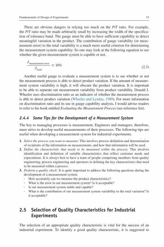
There are obvious dangers in relying too much on the P/T ratio. For example, the P/T ratio may be made arbitrarily small by increasing the width of the specifica-tion of tolerance band. The gauge must be able to have sufficient capability to detect meaningful variation in the product. The contribution of gauge variability (or meas-urement error) to the total variability is a much more useful criterion for determining the measurement system capability. So one may look at the following equation to see whether the given measurement system is capable or not.
ˆ
ˆ%
σ
σmeasurement error
total
1� 0
Another useful gauge to evaluate a measurement system is to see whether or not the measurement process is able to detect product variation. If the amount of measure-ment system variability is high, it will obscure the product variation. It is important to be able to separate out measurement variability from product variability. Donald J. Wheeler uses discrimination ratio as an indicator of whether the measurement process is able to detect product variation (Wheeler and Lynday, 1989). For more information on discrimination ratio and its use in gauge capability analysis, I would advise readers to refer to his book entitled Evaluating the Measurement Process (see reference list).
2.4.4 Some Tips for the Development of a Measurement System
The key to managing processes is measurement. Engineers and managers, therefore, must strive to develop useful measurements of their processes. The following tips are useful when developing a measurement system for industrial experiments.
1. Select the process you want to measure: This involves process definition and determination of recipients of the information on measurements, and how that information will be used.
2. Define the characteristic that needs to be measured within the process: This involves identification and definition of suitable characteristics that reflect customer needs and expectations. It is always best to have a team of people comprising members from quality engineering, process engineering and operators in defining the key characteristics that need to be measured within a process.
3. Perform a quality check: It is quite important to address the following questions during the development of a measurement system:● How accurately can we measure the product characteristics?● What is the error in our measurement system? Is it acceptable?● Is our measurement system stable and capable?● What is the contribution of our measurement system variability to the total variation? Is
it acceptable?
2.5 Selection of Quality Characteristics for Industrial Experiments
The selection of an appropriate quality characteristic is vital for the success of an industrial experiment. To identify a good quality characteristic, it is suggested to
(2.3)

Design of Experiments for Engineers and Scientists16
start with the engineering or economic goal. Having determined this goal, iden-tify the fundamental mechanisms and the physical laws affecting this goal. Finally, choose the quality characteristics to increase the understanding of these mechanisms and physical laws. The following points are useful in selecting the quality character-istics for industrial experiments (Antony, 1998):
● Try to use quality characteristics that are easy to measure.● Quality characteristics should, as far as possible, be continuous variables.● Use quality characteristics which can be measured precisely, accurately and with stability.● For complex processes, it is best to select quality characteristics at the sub-system level
and perform experiments at this level prior to attempting overall process optimisation.● Quality characteristics should cover all dimensions of the ideal function or the input–
output relationship.● Quality characteristics should preferably be additive (i.e. no interaction exists among the
quality characteristics) and monotonic (i.e. the effect of each factor on robustness should be in a consistent direction, even when the settings of factors are changed).
Consider a certain painting process which results in various problems such as orange peel, poor appearance, voids, etc. Too often, experimenters measure these characteristics as data and try to optimise the quality characteristic. It is not the function of the coating process to produce an orange peel. The problem could be due to excess variability of the coating process due to noise factors such as variability in viscosity, ambient tem-perature, etc. We should make every effort to gather data that relate to the engineering function itself and not to the symptom of variability. One fairly good characteristic to measure for the coating process is the coating thickness. It is important to understand that excess variability of coating thickness from its target value could lead to problems such as orange peel or voids. The sound engineering strategy is to design and analyse an experiment so that best process parameter settings can be determined in order to yield a minimum variability of coating thickness around the specified target thickness.
In the context of service organisations, the selection of quality characteristics is not very straightforward due to the human behavioural characteristics present in the delivery of the service. However, it is essential to understand what characteristics can be effi-ciently and effectively measured. For instance, in the banking sector, one may measure the number of processing errors, the processing time for certain transactions, the waiting time to open a bank account, etc. It is important to measure those quality characteristics which have an impact on customer satisfaction. In the context of health care services, one can measure the proportion or fraction of medication errors, the proportion of cases with inaccurate diagnosis, the waiting time to get a treatment, the waiting time to be admitted to an A&E department, the number of malpractice claims in a hospital every week or month, etc.
Exercises
1. What are the three basic principles of DOE?2. Explain the role of randomisation in industrial experiments. What are the limitations of
randomisation in experiments?

Fundamentals of Design of Experiments 17
3. What is replication? Why do we need to replicate experimental trials?4. What is the fundamental difference between repetition and replication?5. Explain the term ‘degrees of freedom’.6. An experimenter wants to study five process parameters at 2-levels and has decided to
use eight trials. How many degrees of freedom are required for studying all five process parameters?
7. What is confounding and what is its role in the selection of a particular design matrix or experimental layout?
8. What is design resolution? Briefly illustrate its significance in industrial experiments.9. What is the role of a measurement system in the context of industrial experimentation?
10. State three key factors for the selection of quality characteristics for the success of an industrial experiment.
11. What are the three Critical-to-Quality (CTQ) characteristics which you believe to be criti-cal in the eyes of international students who are pursuing a post-graduate course at the University?
References
Antony, J., 1997. A Strategic Methodology for the Use of Advanced Statistical Quality Improvement Techniques (PhD thesis). University of Portsmouth, UK.
Antony, J., 1998. Some key things industrial engineers should know about experimental design. Logistics Inf. Manage. 11 (6), 386–392.
Barker, T.B., 1990. Engineering Quality by Design-Interpreting the Taguchi Approach. Marcel Dekker Inc., New York, USA.
Belavendram, N., 1995. Quality by Design: Taguchi Techniques for Industrial Experimentation. Prentice-Hall, UK.
Bisgaard, S., 1994. Blocking generators for small 2(k-p) designs. J. Qual. Technol. 26 (4), 288–296.
Box, G.E.P., 1990. Must we randomise our experiment? Qual. Eng. 2 (4), 497–502.Kolarik, W.J., 1995. Creating Quality: Concepts, Systems, Strategies and Tools. McGraw-Hill,
USA.Leon, R.V., Shoemaker, A., Tsui, K-L., 1993. Discussion on planning for a designed industrial
experiment. Technometrics 35 (1), 21–24.Montgomery, D.C., Runger, G.C., 1993. Gauge capability and designed experiments – Part 1:
basic methods. Qual. Eng. 6 (1), 115–135.Montgomery, D.C., 2001. Design and Analysis of Experiments. John Wiley & Sons, USA.Roy, K., 2001. Design of Experiments Using the Taguchi Approach. John Wiley & Sons, USA.Vecchio, R.J., 1997. Understanding Design of Experiments. Gardner Publications, USA.Wheeler, D.J., Lynday, R.W., 1989. Evaluating the Measurement Process. SPC Press, USA.

Design of Experiments for Engineers and Scientists. DOI: Copyright © 2014 Jiju Antony. Published by Elsevier Ltd. All rights reserved.
http://dx.doi.org/10.1016/B978-0-08-099417-8.00003-1
Understanding Key Interactions in Processes
3
3.1 Introduction
For modern industrial processes, the interactions between the factors or process parameters are a major concern to many engineers and managers, and therefore should be studied, analysed and understood properly for problem solving and pro-cess optimisation problems. For many process optimisation problems in industries, the root cause of the problem is sometimes due to the interaction between the factors rather than the individual effect of each factor on the output performance character-istic (or response). Here performance characteristic is the characteristic of a product/service which is most critical to customers (Logothetis, 1994).
The significance of interactions in manufacturing processes can be illustrated by the following example taken from a wave-soldering process of a PCB assembly line in a certain electronic industry. The engineering team of the company was interested in reducing the number of defective solder joints obtained from the soldering pro-cess. The average defect rate based on the existing conditions is 410 ppm (parts per million). The team has decided to perform a simple experiment to understand the influence of wave-soldering process parameters on the number of defective solder joints.
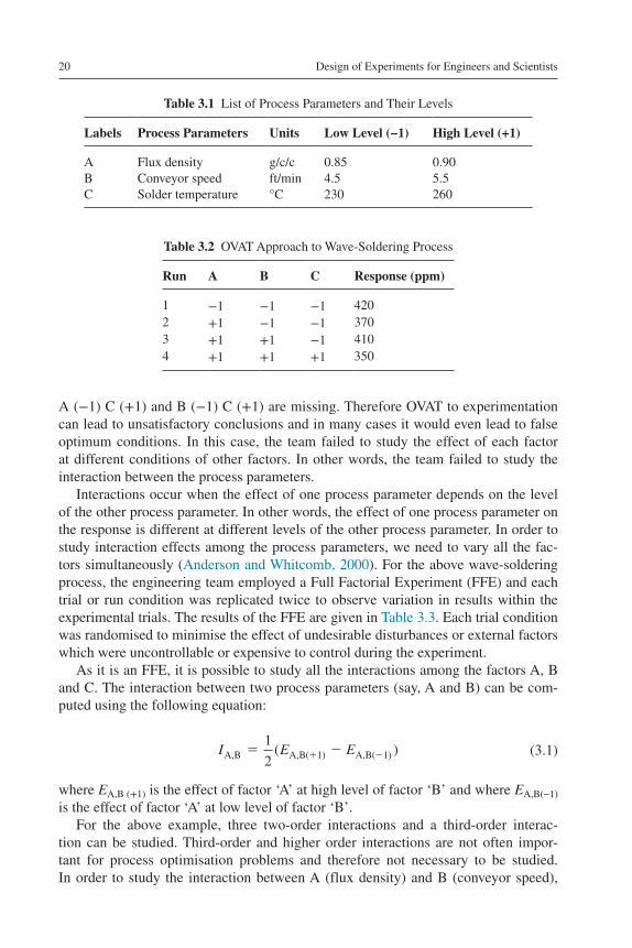
The team initially utilised an OVAT approach to experimentation. Each process parameter (or process variable) was studied at 2-levels – low level (represented by −1) and high level (represented by +1). The parameters and their levels are given in Table 3.1. The experimental layout (or design matrix) for the experiment is given in Table 3.2. The design matrix shows all the possible combinations of factors at their respective levels.
In the experimental layout, the actual process parameter settings are replaced by −1 and +1. The first trial in Table 3.2 represents the current process settings, with each process parameter kept at low level. In the second trial, the team has changed the level of factor ‘A’ from low to high, keeping the levels of other two factors con-stant. The engineer notices from this experiment that the defect rate is minimum, corresponding to trial condition 4, and thereby conclude that the optimal setting is the one corresponding to the fourth trial.
The difference in the responses between the trials 1 and 2 provides an estimate of the effect of process parameter ‘A’. From Table 3.2, the effect of ‘A’ (370 − 420 = −50) was estimated when the levels of ‘B’ and ‘C’ were at low levels. There is no guarantee whatsoever that ‘A’ will have the same effect for different conditions of ‘B’ and ‘C’. Similarly, the effects of ‘B’ and ‘C’ can be estimated. In the above experiment, the response values corresponding to the combinations A (−1) B (+1),
Design of Experiments for Engineers and Scientists20
A (−1) C (+1) and B (−1) C (+1) are missing. Therefore OVAT to experimentation can lead to unsatisfactory conclusions and in many cases it would even lead to false optimum conditions. In this case, the team failed to study the effect of each factor at different conditions of other factors. In other words, the team failed to study the interaction between the process parameters.
Interactions occur when the effect of one process parameter depends on the level of the other process parameter. In other words, the effect of one process parameter on the response is different at different levels of the other process parameter. In order to study interaction effects among the process parameters, we need to vary all the fac-tors simultaneously (Anderson and Whitcomb, 2000). For the above wave-soldering process, the engineering team employed a Full Factorial Experiment (FFE) and each trial or run condition was replicated twice to observe variation in results within the experimental trials. The results of the FFE are given in Table 3.3. Each trial condition was randomised to minimise the effect of undesirable disturbances or external factors which were uncontrollable or expensive to control during the experiment.
As it is an FFE, it is possible to study all the interactions among the factors A, B and C. The interaction between two process parameters (say, A and B) can be com-puted using the following equation:
I E EA,B A,B A,B1
2 1 1( )( ) ( )
where EA,B (+1) is the effect of factor ‘A’ at high level of factor ‘B’ and where EA,B(−1) is the effect of factor ‘A’ at low level of factor ‘B’.
For the above example, three two-order interactions and a third-order interac-tion can be studied. Third-order and higher order interactions are not often impor-tant for process optimisation problems and therefore not necessary to be studied. In order to study the interaction between A (flux density) and B (conveyor speed),
(3.1)
Table 3.1 List of Process Parameters and Their Levels
Labels Process Parameters Units Low Level (−1) High Level (+1)
A Flux density g/c/c 0.85 0.90B Conveyor speed ft/min 4.5 5.5C Solder temperature °C 230 260
Table 3.2 OVAT Approach to Wave-Soldering Process
Run A B C Response (ppm)
1 −1 −1 −1 4202 +1 −1 −1 3703 +1 +1 −1 4104 +1 +1 +1 350

Understanding Key Interactions in Processes 21
it is important to form a table (Table 3.4) for average ppm values at the four possible combinations of A and B (i.e. A(−1) B(−1), A(−1) B(+1), A(+1) B(−1) and A(+1) B(+1)).
From Table 3.4, the effect of ‘A’ (i.e., going from low level (–1) to high level
( ) )) . .
.
+ +1 1 0at high level of B(i.e. 378 75 311 5
67 25ppm
Similarly, the effect of Aat low level of B 4 9 25 398 75
1 5ppm
0
0
. .
.
Interaction between Aand B1
267 25 10 5
28 375
[ . . ]
.
In order to determine whether two process parameters are interacting or not, one can use a simple but powerful graphical tool called interaction graphs. If the lines in the interaction plot are parallel, there is no interaction between the process param-eters (Barton, 1990). This implies that the change in the mean response from low to high level of a factor does not depend on the level of the other factor. On the other hand, if the lines are non-parallel, an interaction exists between the factors. The
Table 3.3 Results from a 23 FFE
Run (Standard Order)
Run (Randomised Order)
A B C Response (ppm)
1 5 −1 −1 −1 420, 4122 7 +1 −1 −1 370, 3753 4 −1 +1 −1 310, 2894 1 +1 +1 −1 410, 4155 8 −1 −1 +1 375, 3886 3 +1 −1 +1 450, 4427 2 −1 +1 +1 325, 3228 6 +1 +1 +1 350, 340
Table 3.4 Average ppm Values
Run (Standard Order)
A B Average ppm
1, 5 −1 −1 398.753, 7 −1 +1 311.502, 6 +1 −1 409.254, 8 +1 +1 378.75

Design of Experiments for Engineers and Scientists22
greater the degree of departure from being parallel, the stronger the interaction effect (Antony and Kaye, 1998). Figure 3.1 illustrates the interaction plot between ‘A’ (flux density) and ‘B’ (conveyor speed).
The interaction graph between flux density and conveyor speed shows that the effect of conveyor speed on ppm at two different levels of flux density is not the same. This implies that there is an interaction between these two process parameters. The defect rate (in ppm) is minimum when the conveyor speed is at high level and flux density at low level.
3.2 Alternative Method for Calculating the Two-Order Interaction Effect
In order to compute the interaction effect between flux density and conveyor speed, we need to first multiply columns 2 and 3 in Table 3.4. This is illustrated in Table 3.5. In Table 3.5, column 3 yields the interaction between flux density (A) and conveyor speed (B).
Having obtained column 3, we then need to calculate the average ppm at high level of (A × B) and low level of (A × B). The difference between these will provide an estimate of the interaction effect.
A B Average ppm at high level of A B Average ppm at low level of (A( ) BB)
(1
2398 75 378 75
1
2311 50 409 25
388 75 360 375
28
. . ) ( . . )
. .
.3375
1–1
410
400390380370360
350340330320310
Conveyor speed
Mea
n
–11
Flux density
Figure 3.1 Interaction plot between flux density and conveyor speed.

Understanding Key Interactions in Processes 23
Now consider the interaction between flux density (A) and solder temperature. The interaction graph is shown in Figure 3.2. The graph shows that the effect of solder temperature at different levels of flux density is almost the same. Moreover, the lines are almost parallel, which indicates that there is little interaction between these two factors.
The interaction plot suggests that the mean solder defect rate is minimum when solder temperature is at high level and flux density at low level.Note: Non-parallel lines are an indicator of the existence of interactions between
two factors and parallel lines indicate no interactions between the factors.
3.3 Synergistic Interaction Versus Antagonistic Interaction
The effects of process parameters can be either fixed or random. Fixed process parameter effects occur when the process parameter levels included in the experi-ment are controllable and specifically chosen because they are the only ones for which inferences are desired. For example, if you want to determine the effect of
Table 3.5 Alternative Method to Compute the Interaction Effect
A B A × B Average ppm
−1 −1 +1 398.75−1 +1 −1 311.50+1 −1 −1 409.25+1 +1 +1 378.75
–1 1
355
365
375
385
395
Solder temperature
Mea
n
–11
Flux density
Figure 3.2 Interaction plot between solder temperature and flux density.
Design of Experiments for Engineers and Scientists24
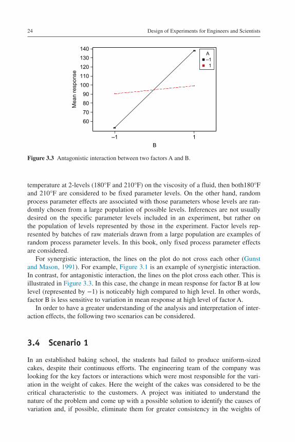
temperature at 2-levels (180°F and 210°F) on the viscosity of a fluid, then both180°F and 210°F are considered to be fixed parameter levels. On the other hand, random process parameter effects are associated with those parameters whose levels are ran-domly chosen from a large population of possible levels. Inferences are not usually desired on the specific parameter levels included in an experiment, but rather on the population of levels represented by those in the experiment. Factor levels rep-resented by batches of raw materials drawn from a large population are examples of random process parameter levels. In this book, only fixed process parameter effects are considered.
For synergistic interaction, the lines on the plot do not cross each other (Gunst and Mason, 1991). For example, Figure 3.1 is an example of synergistic interaction. In contrast, for antagonistic interaction, the lines on the plot cross each other. This is illustrated in Figure 3.3. In this case, the change in mean response for factor B at low level (represented by −1) is noticeably high compared to high level. In other words, factor B is less sensitive to variation in mean response at high level of factor A.
In order to have a greater understanding of the analysis and interpretation of inter-action effects, the following two scenarios can be considered.
3.4 Scenario 1
In an established baking school, the students had failed to produce uniform-sized cakes, despite their continuous efforts. The engineering team of the company was looking for the key factors or interactions which were most responsible for the vari-ation in the weight of cakes. Here the weight of the cakes was considered to be the critical characteristic to the customers. A project was initiated to understand the nature of the problem and come up with a possible solution to identify the causes of variation and, if possible, eliminate them for greater consistency in the weights of
1–1
140
130
120
110
100
90
80
70
60
B
Mea
n re
spon
se
–11
A
Figure 3.3 Antagonistic interaction between two factors A and B.

Understanding Key Interactions in Processes 25
these cakes. Further to a thorough brainstorming session, six process variables (or factors) and a possible interaction (B × M) were considered for the experiment. The factors and their levels are given in Table 3.6.
Each process variable was kept at 2-levels and the objective of the experiment was to determine the optimum combination of process variables which yield mini-mum variation in the weight of cakes. An FFE would have required 64 experimental runs. Due to limited time and experimental budget, it was decided to select a 2(6−3) fractional factorial experiment (i.e. eight trials or runs). Each trial condition was replicated twice to obtain sufficient degrees of freedom for the error term. Because we are analysing variation, the minimum number of replicates per trial condition is two. Table 3.7 presents the experimental layout or design matrix for the cake baking experiment. According to the Central Limit Theorem (CLT), if you repeatedly take large random samples from a stable process and display the averages of each sam-ple in a frequency diagram, the diagram will be approximately bell-shaped. In other words, the sampling distribution of means is roughly normal, according to CLT. It is quite interesting to note that the distribution of sample standard deviations (SDs) does not follow a normal distribution. However, if we transform the sample SDs by taking their logarithms, the logarithms of the SDs will be much closer to being normally distributed. The last column in Table 3.7 gives the logarithmic transforma-tion of sample SD. The SDs and log(SD) can easily be obtained by using a scientific
Table 3.6 List of Baking Process Variables for the Experiment
Factors Label Low Level High Level
Butter (cups) B ¼ ½Milk (cups) M ¼ ½Flour (cups) F ¾ 1Sugar (cups) S ½ ¾Oven temperature (°C) O 200 225Eggs E 2 3
Table 3.7 Response Table for the Cake Baking Experiment
Run B M B × M O F S E Weight (Grams)
log(SD)
1 −1 −1 +1 −1 +1 +1 −1 102.3, 117.6 1.0342 +1 −1 −1 −1 −1 +1 +1 114.6, 120.3 0.6053 −1 +1 −1 −1 +1 −1 +1 134.6, 126.7 0.7474 +1 +1 +1 −1 −1 −1 −1 116.4, 123.9 0.7255 −1 −1 +1 +1 −1 −1 +1 112.6, 130.6 1.1056 +1 −1 −1 +1 +1 −1 −1 150.6, 141.7 0.7997 −1 +1 −1 +1 −1 +1 −1 133.6, 122.4 0.8998 +1 +1 +1 +1 +1 +1 +1 155.8, 138.6 1.085

Design of Experiments for Engineers and Scientists26
calculator or Microsoft Excel spreadsheet. Here our interest is to analyse the interac-tion between the process variables butter (B) and milk (M) rather than the individual effect of each process variable on the variability of cake weights.
In order to analyse the interaction effect between butter and milk, we form a table for average log(SD) values corresponding to all of the four possible combinations of B and M. The results are given in Table 3.8.
Calculation of interaction effect (B × M):
Effect of butter B at high level of milk (M)( ) . . .0 905 0 823 0 082
Using Eq. (4.1),
B M / 82 3675 2251
20 082 0 3675 1 2 0 0 0 0[ . ( . )] [ . . ] .=
Figure 3.4 illustrates the interaction plot between the process variables ‘B’ and ‘M’.Figure 3.4 clearly indicates the existence of interaction between the factors butter
and milk. The interaction plot shows that variability in the weight of cakes is mini-mum when the level of butter is kept at high level and milk at low level.
Effect of butter B at low level of milk (M)( ) . . .0 702 1 0695 0 3675
Table 3.8 Interaction Table for log(SD)
B M Average log(SD)
−1 −1 1.0695−1 +1 0.823+1 −1 0.702+1 +1 0.905
–1 1
0.7
0.8
0.9
1.0
M
Mea
n Lo
g(s)
–11
B
Figure 3.4 Interaction plot between milk and butter.

Understanding Key Interactions in Processes 27
3.5 Scenario 2
In this scenario, we illustrate an experiment conducted by a chemical engineer to study the effect of three process variables (temperature, catalyst and pH) on the chemical yield. The results of the experiment are given in Table 3.9. The engineer was interested in studying the effect of three process variables and the interaction between temperature and catalyst. The engineer has replicated each trial condi-tion three times to obtain sufficient degrees of freedom for the experimental error. Moreover, replication increases the precision of the experiment by reducing the SDs used to estimate the process parameter (or factor) effects.
The first step was to construct a table (Table 3.10) for interaction between TE and CA. The mean chemical yield at all four combinations of TE and CA was estimated. In order to determine whether or not these variables are interacting, an interaction plot was constructed (Figure 3.5).
As the lines are not parallel, there is an interaction between the process varia-bles CA and TE. The graph indicates that the effect of CA is insensitive to mean yield at low level of TE. However, maximum yield is obtained when temperature is kept at a high level. Maximum yield is obtained when temperature is set at a high level and CA at a low level. The interaction effect can be computed in the following manner.
Table 3.9 Experimental Layout for the Yield Experiment
Trial TE CA pH Chemical Yield (%)
1 −1 −1 −1 60.4, 62.1, 63.42 +1 −1 −1 64.1, 79.4, 74.03 −1 +1 −1 59.6, 61.2, 57.54 +1 +1 −1 66.7, 67.3, 68.95 −1 −1 +1 63.3, 66.0, 65.36 +1 −1 +1 91.2, 77.4, 84.97 −1 +1 +1 68.1, 71.3, 68.68 +1 +1 +1 75.3, 77.1, 76.1
Table 3.10 TE × CA Interaction Table
TE CA Mean Chemical Yield
−1 −1 63.42+1 −1 78.50−1 +1 64.38+1 +1 71.90

Design of Experiments for Engineers and Scientists28
Effect of CA at high level of
Effect of CA at low level of
3.6 Scenario 3
In this scenario, we share the results of an experiment carried out in a certain grind-ing process to reduce common-cause variation (random in nature and expensive to control in many cases). The primary purpose of the experiment in this case was to reduce variation in the outer diameter produced by a grinding operation. The follow-ing factors and their effects were of interest to the experimenter.
1. Feed Rate – Factor A – labelled as FR2. Wheel Speed – Factor B – labelled as WHS3. Work Speed – Factor C – labelled as WOS4. Wheel Grade – Factor D – labelled as WG5. Interaction between WHS and WOS6. Interaction between WHS and WG
The results of the experiment are given in Table 3.11. The response of interest for this experiment was Signal-to-Noise ratio (SNR). SNR is a performance statistic recommended by Dr Taguchi in order to make the process insensitive to undesirable disturbances called noise factors (Gijo, 2005; Lochner and Matar, 1990). The pur-pose of the SNR is to maximise the signal while minimising the impact of noise. The whole idea is to achieve robustness, and the higher the SNR, the greater the robust-ness will be.
TE 71 90 78 50 6 60. . .
TE 64 38 63 42 0 96. . .
CA TE 6 6 961
20 0 3 78[ . . ] .
1–1
75
70
65
CA
Mea
n Y
ield
–11
TE
Figure 3.5 Interaction plot between CA and TE.

Understanding Key Interactions in Processes 29
The mean SNR at high level (+1) of WHS × WOS = 51.11The mean SNR at low level (−1) of WHS × WOS = 48.054Therefore, interaction effect = 3.056Similarly, the mean SNR at high level of WHS × WG = 49.409The mean SNR at low level of WHS × WG = 49.754Therefore, interaction effect= −0.345Figure 3.6 illustrates the interaction plot between the WHS and WOS. As the lines
are non-parallel, there is a strong interaction between those two factors.Figure 3.6 shows that the effect of WOS on SNR at different levels of WHS is
not the same. As SNR needs to be maximised, the optimum combination is when WOS and WHS are kept at a low level. Figure 3.7 illustrates the interaction plot between the WHS and WG. As the lines exhibit near parallelism, there is no interac-tion between those two factors.
Table 3.11 SNR Values and Interactions
Trial WHS × WOS WHS × WG Response (SNR)
1 +1 +1 53.4692 −1 −1 50.9703 −1 +1 49.0304 +1 −1 56.9915 +1 +1 49.0306 −1 −1 46.1087 −1 +1 46.1088 +1 −1 44.948
WOS
Mea
n
1–1
51.5
51.0
50.5
50.0
49.5
49.0
48.5
48.0
47.5
Interaction Plot (data means) for SNR
WHS–11
Figure 3.6 Interaction plot between WOS and WHS.

Design of Experiments for Engineers and Scientists30
Exercises
1. In a certain casting process for manufacturing jet engine turbine blades, the objective of the experiment is to determine the most important interaction effects (if there are any) that affect part shrinkage. The experimenter has selected three process parameters: pour speed (A), metal temperature (B) and mould temperature(C), each factor being kept at two lev-els for the study. The response table, together with the response values, is shown below. Calculate and analyse the two-factor interactions among the three process variables. Each run was replicated three times to have adequate degrees of freedom for error.
Run A B C Shrinkage
1 −1 −1 −1 2.22, 2.11, 2.142 +1 −1 −1 1.42, 1.54, 1.053 −1 +1 −1 2.25, 2.31, 2.214 +1 +1 −1 1.00, 1.38, 1.195 −1 −1 +1 1.73, 1.86, 1.796 +1 −1 +1 2.71, 2.45, 2.467 −1 +1 +1 1.84, 1.76, 1.708 +1 +1 +1 2.27, 2.69, 2.71
2. A company that manufactures can-forming equipment wants to set up an experiment to help understand the factors influencing surface finish on a particular steel subassembly. The company decides to perform an eight-trial experiment with three factors at 2-levels. A brainstorming session conducted with people within the organisation ‒ operator, supervisor and engineer ‒ resulted in the finished part being measured at four places. The list of fac-tors (A: tool radius, B: feed rate and C: Revolutions per Minute (RPM)) and the response
WG
Mea
n
1–1
51.5
51.0
50.5
50.0
49.5
49.0
48.5
48.0
47.5
Interaction Plot (data means) for SNR
WHS–11
Figure 3.7 Interaction plot between WG and WHS.

Understanding Key Interactions in Processes 31
(surface finish) is shown in the following experimental layout. Generate an interaction plot for any two-way interactions with large effects.
Run A B C Surface Finish
1 −1 −1 −1 50, 50, 55, 502 +1 −1 −1 145, 150, 100, 1103 −1 +1 −1 160, 165, 155, 1604 +1 +1 −1 180, 200, 190, 1955 −1 −1 +1 60, 65, 55, 606 +1 −1 +1 25, 35, 35, 307 −1 +1 +1 160, 160, 150, 1658 +1 +1 +1 80, 70, 75, 80
3. Assume you are planning to carry out an experiment to investigate the sensitivity of an amplifier to process variation. The response of interest for the experiment is the gain of the amplifier measured in decibels (dB). You would like to evaluate the effects of three factors: resistor (R), width of the microstrip lines (W) and a capacitor (C). Each factor was studied at 2-levels and a simulation was conducted for studying all the combinations of factors at their respective levels. The coded matrix is shown below.
Run W R C Gain (dB)
1 −1 −1 −1 12.852 +1 −1 −1 13.013 −1 +1 −1 14.524 +1 +1 −1 14.715 −1 −1 +1 12.936 +1 −1 +1 13.097 −1 +1 +1 14.618 +1 +1 +1 14.81
Calculate and analyse all the two-factor interactions W × R, R × C and W × C. Also construct an interaction graph between W and R. How would you interpret this graph?
References
Anderson, M.J., Whitcomb, P.J., 2000. DOE Simplified: Practical Tools for Effective Experimentation. Productivity Inc., Portland, OR.
Antony, J., Kaye, M., 1998. Key interactions. Manuf. Eng. 77 (3), 136–138.Barton, R., 1990. Graphical Methods for the Design of Experiments. Springer-Verlag,
New York, NY.

Design of Experiments for Engineers and Scientists32
Gijo, E.V., 2005. Improving process capability of manufacturing process by application of sta-tistical techniques. Qual. Eng. 17 (2), 309–315.
Gunst, R.F., Mason, R.L., 1991. How to Construct Fractional Factorial Experiments. ASQC Quality Press, Milwaukee, WI.
Lochner, R.H., Matar, J.E., 1990. Designing for Quality – An Introduction to the Best of Taguchi and Western Methods of Experimental Design. Chapman and Hall Publishers, USA. New Jersey, NJ.
Logothetis, N., 1994. Managing for Total Quality. Prentice-Hall, London, UK.

Design of Experiments for Engineers and Scientists. DOI: Copyright © 2014 Jiju Antony. Published by Elsevier Ltd. All rights reserved.
http://dx.doi.org/10.1016/B978-0-08-099417-8.00004-3
A Systematic Methodology for Design of Experiments
4
4.1 Introduction
It is widely considered that DOE (or experimental design) forms an essential part of the quest for effective improvement in process performance or product/service qual-ity. This chapter discusses the barriers and cognitive gaps in the statistical knowledge required by industrial engineers for tackling process and quality-related problems using DOE technique. This chapter also presents a systematic methodology to guide people in organisations with limited statistical ability for solving manufacturing pro-cess-related problems in real-life situations.
4.2 Barriers in the Successful Application of DOE
Although DOE has been around for nearly 100 years, research has clearly demon-strated that less than 30% of people are knowledgeable about DOE. Despite every effort by specialists and practitioners in quality and statistics, DOE has yet to be applied as widely as it could and should be. A study carried out in Sweden has shown that only 18% of Swedish companies are using the Robust Parameter Design (RPD) methodology advocated by Dr Taguchi. These results were part of a large study carried out as part of a European project which looked into the use of RPD methodology across five countries (Germany, Ireland, The Netherlands, Spain and Sweden). It was also found that the application of Six Sigma methodology has a pos-itive influence on the application of DOE. A recent study has shown that over 60% of companies that apply DOE frequently are knowledgeable about Six Sigma as a problem-solving methodology. It has been observed over the years that companies utilising Six Sigma and Design for Six Sigma (DFSS) methodologies are using DOE more frequently than those companies which are not. The ‘effective’ application of DOE by industrial engineers is limited in many manufacturing organisations (Antony and Kaye, 1995). Some noticeable barriers are as folows:
● Educational barriersThe word ‘statistics’ invokes fear in many industrial engineers. The fundamental problem begins with the current statistical education for the engineering community in their aca-demic curriculum. The courses currently available in ‘engineering statistics’ often tend to concentrate on the theory of probability, probability distributions and more mathemati-cal aspects of the subject, rather than practically useful techniques such as DOE, Taguchi

Design of Experiments for Engineers and Scientists34
method, robust design, gauge capability studies, Statistical Process Control (SPC), etc. It was found from various sources of literature that DOE is rarely taught at universities or at company-provided training sessions. The best way to tackle this issue is through inces-sant cooperation between industry and academia. In the context of small and medium enterprises (SMEs), engineers typically do not have access to books and case studies which demonstrate the power of DOE. In addition, most of the DOE material is availa-ble in English but many engineers and scientists in the developing world lack adequate English reading skills and therefore cannot use such materials. Another study has shown that the only experiments students participate in, if any, are based on demonstration and are often of limited educational value. Although DOE is a very powerful technique for prob-lem solving in manufacturing companies, it was observed that both engineers and scientists receive little or no training in DOE at the university level. The most common criticisms of the teaching of DOE in many schools are that it is too academic in focus and that most examples taught to engineers are far too theoretical and do not represent real-world prob-lems. There is a clear consensus that academics needs to change the way it teaches busi-ness statistics (Bisgaard, 1991). Engineers must be taught these powerful techniques in the academic world with a number of supporting case studies. This will ensure a better under-standing of the application of statistical techniques before they enter the job market.
● Management barriersManagers often don’t understand the importance of DOE in problem solving or don’t appreciate the competitive value it brings into the organisation. In many organisations, managers encourage their engineers to use the so-called ‘home-grown’ solutions for pro-cess- and quality-related problems. These ‘home-grown’ solutions are consistent with the OVAT approach to experimentation, as managers are always after quick-fix solutions which yield short-term benefits to their organisations. Responses from managers with high resistance to change may include the following:● DOE tells me what I already know.● It sounds good, but it is not applicable to my job.● I need to make additional effort to prove what I already know.
Many managers do not instinctively think statistically, mainly because they are not convinced that statistical thinking adds any value to management and decision-making. Managers in organisations believe that DOE is very demanding of resources.
● Cultural barriersCultural barriers are one of the principal reasons why DOE is not commonly used in many organisations. The management should be prepared to address all cultural barrier issues that might be present within the organisation, plus any fear of training or reluctance to embrace the application of DOE. Many organisations are not culturally ready for the intro-duction and implementation of advanced quality improvement techniques such as DOE and Taguchi. The best way to overcome this barrier is through intensive training programs and by demonstrating the successful application of such techniques by other organisations during the training. The culture of the company is very much reliant on the style of lead-ership. If the leaders are not committed to the idea of performing industrially designed experiments for improving quality and process efficiency, then the concept of DOE becomes just ‘lip service’ on the part of the senior management team and will never be a reality (Tanco et al., 2009).
● Communication barriersResearch has indicated that there is very little communication between the academic and industrial worlds. Moreover, the communication among industrial engineers, managers

A Systematic Methodology for Design of Experiments 35
and statisticians in many organisations is limited. For the successful initiative of any quality improvement programme, these communities should work together and make this barrier less formidable. For example, lack of statistical knowledge for engineers could lead to problems such as misinterpretation of historical data or misunderstanding of the nature of interactions among factors under consideration for a given experiment. Similarly, academic statisticians’ lack of engineering knowledge could lead to problems such as undesirable selection of process variables and quality characteristics for the experi-ment, lack of measurement system precision and accuracy, etc. Managers’ lack of basic knowledge in engineering and statistics could lead to problems such as high quality costs, poor quality and therefore lost competitiveness in the world marketplace and so on and so forth.
● Other barriersNegative experiences with DOE may make companies reluctant to use DOE again. The majority of negative DOE experiences can be classified into two groups. The first relates to technical issues and the second to non-technical issues. Technical issues include● choosing unreasonably large or small designs;● inadequate or even poor measurement of quality characteristics;● not choosing the appropriate levels for the process variables, etc. Non-linearity or cur-
vature effects of process variables should be explored to determine the best operating process conditions;
● assessing the impact of ‘uncontrolled variables’ which can influence the output of the process. Experimenters should try to understand how the ‘uncontrolled variables’ influ-ence the process behaviour and devise strategies to minimise their impact as much as possible; and
● lacking awareness of assumptions: data analysis, awareness of different alternatives whey they are needed, etc.
Some of the non-technical issues include● lack of experimental planning;● executing one-shot experimentation instead of adopting sequential, adaptive and itera-
tive nature of experimentation and● not choosing the right process variables or design variables for the experiment in the
first round of experimentation, etc.
Commercial software systems and expert systems in DOE provide no guidance whatsoever in classifying and analysing manufacturing process quality-related problems from which a suitable approach (Taguchi, Classical or Shainin’s approach) can be selected. Very little research has been done on this particular aspect and from the author’s standpoint, this is probably the most important part of DOE. The selection of a particular approach to experimentation (i.e. Taguchi, Classical or Shainin) is dependent upon a number of criteria: the complexity involved, the degree of optimisation required by the experimenter, the time required for completion of the experiment, cost issues associated with the experiment, the allowed response time to report back to management, etc. Moreover, many software systems in DOE stress data analysis and do not properly address data interpretation. Thus, many engineers, having performed the statistical analysis using such software systems, would not know how to effectively utilise the results of the analysis without assistance from statisticians.

Design of Experiments for Engineers and Scientists36
4.3 A Practical Methodology for DOE
The methodology of DOE is fundamentally divided into four phases. These are:
1. planning phase2. designing phase3. conducting phase4. analysing phase.
4.3.1 Planning Phase
The planning phase is made up of the following steps. Many engineers pay special attention on the statistical details of DOE and very little attention to the non-statis-tical details. According to Peace (1993), experimental studies may fail not only as a result of lack of technical knowledge of the process under study or wrong use of statistical techniques but also due to lack of planning. It is the responsibility of the senior management team in the organisation to create an environment that stimulates a culture of using experimental design techniques for process optimisation problems, product and process development projects, improving process capability through systematically reducing excessive variation in processes, etc.
Problem Recognition and Formulation
A clear and succinct statement of the problem can create a better understanding of what needs to be done. The statement should contain an objective that is specific, measurable and which can yield practical value to the company (Kumar and Tobin, 1990). The creation of a multidisciplinary team in order to have a shared under-standing of the problem is critical in the planning phase. The multidisciplinary team should be led by someone with good knowledge of the process (a DOE specialist), good communication skills, good interpersonal skills and awareness of team dynam-ics. Other team members may include process engineers, a quality engineer/manager, a machine operator, a management representative and manufacturing/production engineers/managers. Sharing experiences and individual knowledge is critical to assure a deeper understanding of the process providing more efficient ways to design experiments (Romeu, 2006). Some manufacturing problems that can be addressed using an experimental approach include
● development of new products; improvement of existing processes or products;● improvement of the process/product performance relative to the needs and demands of
customers;● reduction of existing process spread, which leads to poor capability.
The objective of the experiment must be clearly specified and has to be measur-able. Objectives can be either short term or long term. A short-term objective could be to fix a problem related to a high scrap rate. However, this objective is not at all specific and not measured in a true sense. What is ‘high’, for instance? What particu-lar process causes a high scrap rate? Some aspects of Six Sigma thinking would be

A Systematic Methodology for Design of Experiments 37
very beneficial to help the team convert this engineering or manufacturing problem into a statistical problem.
Selection of Response or Quality Characteristic
The selection of a suitable response for the experiment is critical to the success of any industrially designed experiment. Time spent in establishing a meaningful response variable before a well-planned experiment is rarely wasted. The response can be variable or attribute in nature. Variable responses such as length, thickness, diameter, viscosity, strength, etc. generally provide more information than attribute responses such as good/bad, pass/fail or yes/no. Moreover, variable characteristics or responses require fewer samples than attributes to achieve the same level of statisti-cal significance. It is also not unusual to have several responses requiring simultane-ous optimisation, which can be quite challenging at times.
Experimenters should define the measurement system prior to performing the experiment in order to understand what to measure, where to measure and who is doing the measurements, etc. so that various components of variation (measure-ment system variability, operator variability, part variability, etc.) can be evaluated. Defining a measurement system, including human resources, equipments and meas-urement methods, is a fundamental aspect in planning experimental studies. It is important to ensure that equipment exists and is suitable, accessible and calibrated. The quality of a measurement system is usually determined by the statistical prop-erties of the data it generates over a period of time which captures both long- and short-term variation. Experimenters should be aware of the repeatability, reproduci-bility and uncertainty of the measurements prior to the execution of industrial experi-ments (Launsby and Weese, 1995). It is advisable to make sure that the measurement system is capable, stable, robust and insensitive to environmental changes.
Selection of Process Variables or Design Parameters
Some possible ways to identify potential process variables are the use of engineering knowledge of the process, historical data, cause-and-effect analysis and brainstorm-ing. This is a very important step of the experimental design procedure. If important factors are left out of the experiment, then the results of the experiment are not accu-rate or useful for any improvement actions. It is a good practice to conduct a screen-ing experiment in the first phase of any experimental investigation to identify the most important design parameters or process variables. More information on screen-ing experiments/designs can be obtained from Chapter 5.
Classification of Process Variables
Having identified the process variables, the next step is to classify them into con-trollable and uncontrollable variables. Control variables are those which can be controlled by a process engineer/production engineer in a production environ-ment. Uncontrollable variables (or noise variables) are those which are difficult or expensive to control in actual production environments. Variables such as ambient

Design of Experiments for Engineers and Scientists38
temperature fluctuations, humidity fluctuations, raw material variations, etc. are examples of noise variables. These variables may have an immense impact on the process variability and therefore must be dealt with for enhanced understanding of our process. The effect of such nuisance variables can be minimised by the effective application of DOE principles such as blocking, randomisation and replication. (For more information on these three principles, refer to Chapter 8.)
Determining the Levels of Process Variables
A level is the value that a process variable holds in an experiment. For example, a car’s gas mileage is influenced by such levels as tyre pressure, speed, etc. The num-ber of levels depends on the nature of the process variable to be studied for the experiment and whether or not the chosen process variable is qualitative (type of cat-alyst, type of material, etc.) or quantitative (temperature, speed, pressure, etc.). For quantitative process variables, two levels are generally required in the early stages of experimentation. However, for qualitative variables, more than two levels may be required. If a non-linear function is expected by the experimenter, then it is advisable to study variables at three or more levels. This would assist in quantifying the non-linear (or curvature) effect of the process variable on the response function.
List All the Interactions of Interest
Interaction among variables is quite common in industrial experiments. In order to effectively interpret the results of the experiment, it is highly desirable to have a good understanding of the interaction between two process variables (Marilyn, 1993). The best way to relate to interaction is to view it as an effect, just like a factor or process variable effect. Since it is not an input you can control, unlike factors or process variables, interactions do not enter into descriptions of trial conditions. In the context of DOE, we generally study two-order interactions. The number of two-order interactions within an experiment can be easily obtained by using a simple equation:
Nn n( )1
2
where n is the number of factors.For example, if you consider four factors in an experiment, the number of two-
order interactions can be equal to six.The questions to ask include ‘Do we need to study the interactions in the initial
phase of experimentation?’ and ‘How many two-order interactions are of interest to the experimenter?’ The size of the experiment is dependent on the number of fac-tors to be studied and the number of interactions, which are of great concern to the experimenter.
4.3.2 Designing Phase
In this phase, one may select the most appropriate design for the experiment. Some DOE practitioners would argue that proper experimental design is often more
(4.1)
A Systematic Methodology for Design of Experiments 39
important than sophisticated statistical analysis. The author would agree with this point as the damage caused by poor experimental design is irreparable. The choice of design depends upon a number of factors such as the number of factors to be stud-ied, the number of levels at which the factors are to be explored, the resources and budget allocated for the experiment, the nature of the problem and objectives to be achieved, etc. Experiments can be statistically designed using the classical approach advocated by Sir Ronald Fisher, the orthogonal array approach advocated by Dr Genichi Taguchi or the variables search approach promoted by Dr Dorian Shainin. This book is focused on the classical DOE approach advocated by Sir Ronald Fisher. Within this approach, one can choose full factorial, fractional factorial or screening designs (such as Plackett–Burmann designs). These designs are introduced to the reader in the subsequent chapters.
During the design stage, it is quite important to consider the confounding struc-ture and resolution of the design (Minitab, 2000). It is good practice to have the design matrix ready for the team prior to executing the experiment. The design matrix generally reveals all the settings of factors at different levels and the order of running a particular experiment. Experimenters are advised to carefully consider the three principles of experimental design prior to conducting the real experiment. The principles of randomisation, replication and blocking should be carefully taken into account but depending upon the nature of the problem and the objectives set for the experiment (Montgomery, 2001). These principles will be explained in detail at a later stage of the book.
4.3.3 Conducting Phase
This is the phase in which the planned experiment is carried out and the results are evaluated. Several considerations are recognised as being recommended prior to exe-cuting an experiment, such as
● selection of a suitable location for carrying out the experiment. It is important to ensure that the location is not affected by any external sources of noise (vibration, humidity, etc.);
● availability of materials/parts, operators, machines, etc. required for carrying out the experiment;
● assessment of the viability of an action in monetary terms by utilising cost–benefit analy-sis. A simple evaluation must also be carried out in order to verify that the experiment is the only possible solution for the problem at hand and justify that the benefits to be gained from the experiment will exceed the cost of the experiment.
The following steps may be useful while performing the experiment in order to ensure that it is performed according to the prepared experimental design matrix (or layout).
● The person responsible for the experiment should be present throughout the experiment. In order to reduce the operator-to-operator variability, it is best to use the same operator for the entire experiment.
● Monitor the experimental trials. This is to find any discrepancies while running the experi-ment. It is advisable to stop running the experiment if any discrepancies are found.
● Record the observed response values on the prepared data sheet or directly into the computer.● Any experiment deviations and unusual occurrences must be recorded and analysed.

Design of Experiments for Engineers and Scientists40
4.3.4 Analysing Phase
It has been quite interesting to observe over the years that many engineers rush into the conducting and analysing phases of DOE and pay little attention to the planning and designing phases. My personal message, as a mechanical engineer, to the engi-neering fraternity is that it is the planning and designing phases that are crucial to the success of the experiment and not the executing and analysing phases. I am not sug-gesting that conducting and analysing the phases of DOE are unimportant but if we do not plan and design an experiment correctly the first time, there is no way to save the experiment with a sophisticated statistical analysis.
Having performed the experiment, the next phase is to analyse and interpret the results so that valid and sound conclusions can be derived. In DOE, the following are the possible objectives to be achieved from this phase:
● Determine the design parameters or process variables that affect the mean process performance.
● Determine the design parameters or process variables that influence performance variability.● Determine the design parameter levels that yield the optimum performance.● Determine whether further improvement is possible.
The following tools can be used for the analysis of experimental results. As the focus of this book is to ‘Keep It Statistically Simple’ for the readers, the author will be introducing only simple but powerful tools for the analysis and interpretation of results. There are a number of DOE books available on the market that cover more sophisticated statistical methods for the analysis. The author encourages readers to use Minitab software for the analysis of experimental results.
4.4 Analytical Tools of DOE
4.4.1 Main Effects Plot
A main effects plot is a plot of the mean response values at each level of a design parameter or process variable. One can use this plot to compare the relative strength of the effects of various factors. The sign and magnitude of a main effect would tell us the following:
● The sign of a main effect tells us of the direction of the effect, that is, whether the average response value increases or decreases.
● The magnitude tells us of the strength of the effect.
If the effect of a design or process parameter is positive, it implies that the aver-age response is higher at a high level rather than a low level of the parameter setting. In contrast, if the effect is negative, it means that the average response at the low-level setting of the parameter is more than at the high level. Figure 4.1 illustrates the main effect of temperature on the tensile strength of a steel specimen. As you can see from the figure, tensile strength increases when the temperature setting varies from low to high (i.e. −1 to 1).

A Systematic Methodology for Design of Experiments 41
The effect of a process or design parameter (or factor) can be mathematically cal-culated using the following simple equation:
E F Ff ( ) ( )1 1
where F( )�1 = average response at high-level setting of a factor, and F( )�1 = average response at low-level setting of a factor.
4.4.2 Interactions Plots
An interactions plot is a powerful graphical tool which plots the mean response of two factors at all possible combinations of their settings. If the lines are parallel, this indicates that there is an interaction between the factors. Non-parallel lines are an indication of the presence of interaction between the factors. More information on interactions and how to interpret them can be seen in Chapter 3.
4.4.3 Cube Plots
Cube plots display the average response values at all combinations of process or design parameter settings. One can easily determine the best and worst combina-tions of factor levels for achieving the desired optimum response. A cube plot is use-ful to determine the path of steepest ascent or descent for optimisation problems. Figure 4.2 illustrates an example of a cube plot for a cutting tool life optimisation study with three tool parameters: cutting speed, tool geometry and cutting angle. The graph indicates that tool life increases when cutting speed is set at low level and cut-ting angle and tool geometry are set at high levels. The worst condition occurs when all factors are set at low levels.
4.4.4 Pareto Plot of Factor Effects
The Pareto plot allows one to detect the factor and interaction effects that are most important to the process or design optimisation study one has to deal with. It displays
(4.2)
8.5
9.0
9.5
10.0
10.5–1 1
Temperature
Ten
sile
str
engt
h
Figure 4.1 Main effect plot of temperature on tensile strength.

Design of Experiments for Engineers and Scientists42
the absolute values of the effects, and draws a reference line on the chart. Any effect that extends past this reference line is potentially important. For example, for the above tool life experiment, a Pareto plot is constructed (Figure 4.3). The graph shows that factors B and C and interaction AC are most important. Minitab displays the abso-lute value of the standardised effects of factors when there is an error term. It is always a good practice to check the findings from a Pareto chart with Normal Probability Plot (NPP) of the estimates of the effects (refer to NPP in the following section).
4.4.5 NPP of Factor Effects
For NPPs, the main and interaction effects of factors or process (or design) parameters should be plotted against cumulative probability (%). Inactive main and interaction
42.33354.667
42.333
34.66726.000
49.333
37.667
39.667
–1–1 –1
1
Cutting angle
Cutting speed
Tool geometry
1
1
Figure 4.2 Example of a cube plot for cutting tool optimisation study.
543210
B
AC
C
BC
ABC
AB
A
A: Cutting speedB: Tool geometryC: Cutting angle
Figure 4.3 Pareto plot of the standardised effects.

A Systematic Methodology for Design of Experiments 43
effects tend to fall roughly along a straight line, whereas active effects tend to appear as extreme points falling off each end of the straight line (Benski, 1989). These active effects are judged to be statistically significant. Figure 4.4 shows an NPP of effects of factors for the above cutting tool optimisation example at a 5% significance level. Here the significance level is the risk of saying that a factor is significant when in fact it is not. In other words, it is the probability of the observed significant effect being due to pure chance. The results are absolutely identical to that of a Pareto plot of fac-tor/interaction effects.
4.4.6 NPP of Residuals
One of the key assumptions for the statistical analysis of data from industrial experi-ments is that the data come from a normal distribution. The appearance of a moderate departure from normality does not necessarily imply a serious violation of the assump-tions. Gross deviations from normality are potentially serious and require further analysis. In order to check the data for normality, it is best to construct an NPP of the residuals. NPPs are useful for evaluating the normality of a data set, even when there is a fairly small number of observations. Here residual is the mean difference between the observed value (obtained from the experiment) and the predicted or fitted value. If the residuals fall approximately along a straight line, they are then normally distributed. In contrast, if the residuals do not fall fairly close to a straight line, they are then not nor-mally distributed and hence the data do not come from a normal population.
The general approach to dealing with non-normality situations is to apply vari-ance-stabilising transformation on the data. An explanation on data transforma-tion is beyond the scope of this book and therefore readers are advised to refer to Montgomery (2001), which covers the use of data transformation and how to per-form data transformation in a detailed manner. Figure 4.5 illustrates the NPP of residuals for the cutting tool optimisation example. The graph shows that the points fall fairly close to a straight line, indicating that the data are approximately normal.
–4 –3 –2 –1 0 1 2 3 4 5
–1.5
–1.0
–0.5
0.0
0.5
1.0
1.5
Standardised effect
Nor
mal
sco
re
B
C
AC
A: Cutting speedB: Tool geometryC: Cutting angle
Figure 4.4 NPP of effects for cutting tool optimisation example.

Design of Experiments for Engineers and Scientists44
4.4.7 Response Surface Plots and Regression Models
Response surface plots such as contour and surface plots are useful for establishing desirable response values and operating conditions. In a contour plot, the response surface is viewed as a two-dimensional plane where all points that have the same response are connected to produce contour lines of constant responses. A surface plot generally displays a three-dimensional view that may provide a clearer pic-ture of the response. If the regression model (i.e. first-order model) contains only the main effects and no interaction effect, the fitted response surface will be a plane (i.e. contour lines will be straight). If the model contains interaction effects, the con-tour lines will be curved and not straight. The contours produced by a second-order model will be elliptical in nature. Figures 4.6 and 4.7 illustrate the contour and sur-face plots of cutting tool life (hours).
1050–5
2
1
0
–1
–2
Residual
Nor
mal
sco
re
Figure 4.5 NPP of residuals for the cutting tool example.
313641
–1
–1
0 1
0
1
Cutting speed
Cut
ting
angl
e
Figure 4.6 Contour plot of cutting tool life.

A Systematic Methodology for Design of Experiments 45
Both contour and surface plots help experimenters to understand the nature of the relationship between the two factors (cutting speed and cutting angle) and the response (life in hours). As can be seen in Figures 4.6 and 4.7, the tool life increases with an increase in cutting angle and a decrease in cutting speed. Moreover, we have used a fitted surface (Figure 4.7) to find a direction of potential improvement for a process. A formal way to seek the direction of improvement in process optimisation problems is called the method of steepest ascent or descent (depending on the nature of the problem at hand, i.e. whether one needs to maximise or minimise the response of interest).
4.5 Model Building for Predicting Response Function
This section is focused on the model building and prediction of response function at various operating conditions of the process. Here the author uses a regression model approach to illustrate the relationship between a response and a set of process param-eters (or design parameters) which affect the response. The use of this regression model is to predict the response for different combinations of process parameters (or design parameters) at their best levels. In order to develop a regression model based on the significant effects (either main or interaction), the first step is to deter-mine the regression coefficients. For factors at 2-levels, the regression coefficients are obtained by dividing the estimates of effects by 2. The reason is that a two-unit change (i.e. low-level setting (−1) to a high-level setting (+1)) in a process param-eter (or factor) produces a change in the response function. A regression model for factors at 2-levels is usually of the form
y x x x x x xβ β β β β ε0 1 1 2 2 12 1 2 13 1 3� � (4.3)
1
0–1
25272931333537394143
0Cutting speed
Cutting angle
Life
(ho
urs)
–11
Figure 4.7 Surface plot of cutting tool life.

Design of Experiments for Engineers and Scientists46
where β1, β2 are the regression coefficients and β0 is the average response in a facto-rial experiment. The term ‘ε’ is the random error component which is approximately normal and independently distributed with mean zero and constant variance σ2. The regression coefficient β12 corresponds to the interaction between the process param-eters x1 and x2. For example, the regression model for the cutting tool life optimisa-tion study is given by
ˆ . . ( ) . ( ) . ( )y B C AC40 833 5 667 3 417 4 417
The response values obtained from Eq. (4.4) are called predicted values and the actual response values obtained from the experiment are called observed values. Residuals can be obtained by taking the difference of observed and predicted (or fitted) values. Equation (4.4) provides us with a tool that can be used to study the response as a function of three tool life parameters: cutting speed, tool geometry and cutting angle. We can predict the cutting tool life for various combinations of these tool parameters. For instance, if all the cutting tool life parameters are kept at low-level settings, the predicted tool life then would be
ˆ . . ( ) . ( ) . ( ). . ( ) .
y B C AC40 833 5 667 3 417 4 41740 833 5 667 1 3 4117 1 4 417 1 127 332
( ) . ( ) ( ).
The observed value of tool life (refer to cube plot) is 26 h. The difference between the observed value and predicted value (i.e. residual) is − 1.332. Similarly, if all the cutting tool life parameters are kept at the optimal condition (i.e. cutting speed = low, tool geometry = high and cutting angle = high), the predicted tool life would then be
ˆ . . . { . }.
y 4 883 5 667( 1) 3 417( 1) 4 417( 1) ( 1)54 384
0
Once the statistical analysis is performed on the experimental data, it is important to verify the results by means of confirmatory experiments or trials. The number of confirmatory runs at the optimal settings can vary from 4 to 20 (4 runs if expensive, 20 runs if cheap).
4.6 Confidence Interval for the Mean Response
The statistical confidence interval (CI) (at 99% confidence limit) for the mean response can be computed using the equation
CISD
yn
3
(4.4)
(4.5)

A Systematic Methodology for Design of Experiments 47
wherey = mean response obtained from confirmation trials or runsSD = standard deviation of response obtained from confirmation trialsn = number of samples (or confirmation runs).
For the cutting tool life example, five samples were collected from the process at the optimal condition (i.e. cutting speed = low, tool geometry = high and cutting angle = high). The results of the confirmation trials are illustrated in Table 4.1.
y � �53 71 0 654. .h and SD h
Ninety-nine per cent CI for the mean response is given by:
CI 53 71 30 654
553 71 0 877 54 55 52 83
..
. . ( . , . )
As the predicted value based on the regression model falls within the statistical CI, we will consider our model good.
If the results from the confirmation trials or runs fall outside the statistical CI, possible causes must be identified. Some of the possible causes may be
● incorrect choice of experimental design for the problem at hand● improper choice of response(s) for the experiment● inadequate control of noise factors, which cause excessive variation● omission of some important process or design parameters in the first rounds of experi-
mentation● measurement error● wrong assumptions regarding interactions● errors in conducting the experiment, etc.
If the results from the confirmatory trials or runs are within the CI, then improve-ment action on the process is recommended. The new process or design parameters should be implemented with the involvement of top management. After the solution has been implemented, control charts on the response(s) or key process parameters should be constructed for constantly monitoring, analysing, managing and improving the process performance.
Table 4.1 Confirmation Trials
Results from Confirmation Trials
53.4852.6953.8854.1254.36

Design of Experiments for Engineers and Scientists48
4.7 Statistical, Technical and Sociological Dimensions of DOE
4.7.1 Statistical Dimension of DOE
This dimension refers to all statistical assumptions and mathematical methods that validate the application of DOE. Some of the key aspects one may consider include (Tanco et al., 2008) the following:
● Low precision of the experiment due to inadequate samples collected per experimental run – Quite often engineers in organisations rush into experiments without having a good understanding of the number of replicates they need to have per trial condition. The levels of α and β risks should be understood in the planning phase. Here α is the risk of wrongly deciding that a process variable is a signal in our process when in reality it is not. On the other hand, β represents the risk of missing a signal and considering it as underlying noise. The levels of both risks should be chosen in a way that is both technically acceptable and economically feasible. The number of replicates is related to its power or capability to detect signals; as each experimental run requires resources, there is a trade-off between precision and the allocated budget for the experiment.
● Randomisation is difficult as some of the factors were hard to change – When some of the fac-tors are hard to change, it is good practice to look into ‘split-plot’ design. It is common to forget the split-plot structure of the design and analyse the data as a full factorial design, but this can lead to erroneous conclusions on the determination of significant factors and their interactions.
● Lack of proper analysis of residuals – Some assumptions before we carry out proper statisti-cal analysis must be verified to validate the results of the analysis. Emphasis must be given to independence of the residuals, the variance stability and normality assumption of data.
● Data transformation before the identification of factor effects on the response variable – In DOE, we transform the response variable to stabilise the variance of the residuals and Box–Cox transformation is very useful when little is known about the behaviour of the process.
● Proper analysis of interactions and the confounding pattern – Many engineers in organisa-tions do not have a good understanding of how to analyse interactions and how to interpret the confounding structure provided by statistical software systems. This scenario is very much applicable when engineers are trying to characterise a process using low-resolution design where main effects are confounded with two interaction effects.
4.7.2 Technical Dimension of DOE
Technical dimension refers to the way experiments are executed as well as all activi-ties involved in experimental planning until some realistic conclusions are derived. Technical dimensions include
● Process stability before conducting DOE – A number of scholars debate the point as though experimenters need to achieve process stability prior to performing a designed experiment (Costa et al., 2006). Although randomisation and blocking are principles used to reduce suspected noises in the process, it is advisable to achieve process stability (as much as possible) so that noise factors will not prevent the identification of important fac-tor and interaction effects.

A Systematic Methodology for Design of Experiments 49
● Involvement of key players for identification of factors – It is absolutely critical to involve all the stakeholders at the planning phase in order to reach a consensus on which factors should be included in the experiment. Experiments are always very expensive and time consuming and therefore it is advisable to clearly define the team formation and the roles and responsibilities of all team members.
● Selection of wrong levels and not taking time to explore curvature effects – Selecting the right process variables and choosing the appropriate levels for the process variables is not a straightforward process in industrially designed experiments. Experimenters should be able to explore the curvature effects of process variables to determine if non-linear effects are present. This can be achieved by adding centre points. It is often a good practice to start with 2k factorial or 2(k − p) fractional factorial experiments and then add centre points to determine the presence of curvature effects of process variables on the response or quality characteristic of interest (Anderson and Kraber, 1999).
4.7.3 Sociological and Managerial Dimensions of DOE● DOE in an industrial context is always an iterative process; each experiment answers some
questions and triggers new ones, and so on until the team concludes that the full knowl-edge required is sufficient to reach the expected degree of excellence of the process. Some of the sociological and managerial dimensions include
● Communicating the need for DOE at the Senior Management level – Clear and open com-munication to the senior management team about the need for DOE is a critical factor. It is absolutely essential to share world-class examples to gain the attention of the senior man-agement team.
● Communicating the need for DOE at the shop floor level – Process improvement tech-niques such as DOE are not meant just for senior- and middle-level managers. For DOE to be successful, it is absolutely critical to involve people on the shop floor to identify the potential process variables or factors which are believed to have an impact on the response or quality characteristic. Operators and supervisors on the shop floor can also give good input into the selection of levels for each process variable.
● Using the DOE project charter as a tool to develop a good business case for the prob-lem – Many Six Sigma-related projects in organisations begin with a project charter which encompasses the cost-benefits, the nature of the problem, what to measure in order to describe the problem, how to measure, etc. I do think it might be a good practice for engi-neers and experimenters to develop a DOE project charter at the planning phase and pre-sent it to the senior management team for approval.
Exercises
1. What are the common barriers to the successful application of DOE?2. Discuss the four phases in the methodology of DOE.3. What are the criteria for the selection of an experimental design?4. Explain the key considerations which need to be taken into account prior to executing an
experiment.5. What is the purpose of NPP of residuals?6. Explain the role of Response Surface Plots in industrial experiments.
Design of Experiments for Engineers and Scientists50
7. Why do we need to develop regression models? 8. What are the possible causes of experiments being unsuccessful? 9. What are the statistical dimensions of the execution of an industrially designed experiment?10. What are the technical dimensions of the execution of an industrially designed experiment?11. What are the managerial and sociological dimensions of the execution of an industrially
designed experiment?
References
Anderson, M.J., Kraber, S.L., 1999. Eight keys to successful DOE. Qual. Digest 19 (7), 39–43.
Antony, J., Kaye, M., 1995. A methodology for Taguchi design of experiments for continuous quality improvement. Qual. World Tech. Suppl. September, 98–102.
Bisgaard, S., 1991. Teaching statistics to engineers. Am. Stat. 45 (4), 274–283.Benski, H.C., 1989. Use of a normality test to identify significant effects in factorial designs.
J. Qual. Technol. 21 (3), 174–178.Costa, N.R.P., Pires, A.R., Ribeiro, C.O., 2006. Guidelines to help practitioners of design of
experiments. TQM Mag. 18 (4), 386–399.Kumar, S., Tobin, M., 1990. Design of experiments is the best way to optimise a process at
minimal cost. IEEE/CHMT, 166–173.Launsby, R., Weese, D., 1995. Straight Talk on Designing Experiments. Launsby Consulting,
Colorado Springs, CO.Marilyn, H., 1993. A holistic approach to the design of experiments. ASQC Stat. Div.
Newsletter 13 (3), 16–20.Minitab, February 2000. Statistical Software User Manual, Release 13 for Windows.Montgomery, D.C., 2001. Design and Analysis of Experiments. John Wiley & Sons,
New Jersey, USA.Peace, G.S., 1993. Taguchi Methods: A Hands-on Approach. Addison-Wesley Publishing,
New York, NY.Romeu, J.L., 2006. Teaching Engineering Statistics to Practicing Engineers, ICOTS-7,
Salvador, Brazil.Tanco, M., et al., 2008. Is design of experiments really used? A survey of basque industries. J.
Eng. Des. 19 (5), 447–460.Tanco, M., et al., 2009. Barriers faced by engineers when applying design of experiments.
TQM J. 21 (6), 565–575.

Design of Experiments for Engineers and Scientists. DOI: Copyright © 2014 Jiju Antony. Published by Elsevier Ltd. All rights reserved.
http://dx.doi.org/10.1016/B978-0-08-099417-8.00005-5
Screening Designs5
5.1 Introduction
In many process development and manufacturing applications, the number of poten-tial process or design variables or parameters (or factors) is large. Screening is used to reduce the number of process or design parameters (or factors) by identifying the key ones that affect the product quality or process performance. This reduction allows one to focus process improvement efforts on the few really important factors, or the ‘vital few’.
Screening designs provide an effective way to consider a large number of process or design parameters (or factors) in a minimum number of experimental runs or tri-als (i.e. with minimum resources and budget). The purpose of screening designs is to identify and separate out those factors that demand further investigation. This chap-ter is focused on the Screening Designs expounded by R.L. Plackett and J.P. Burman in 1946 ‒ hence the name Plackett–Burman designs (P–B designs). P–B designs are based on Hadamard matrices in which the number of experimental runs or trials is a multiple of four, i.e. N = 4, 8, 12, 16 and so on, where N is the number of trials/runs (Plackett and Burmann, 1946).
P–B designs are suitable for studying up to k = (N−1)/(L−1) factors, where L is the number of levels and k is the number of factors. For instance, using a 12-run experiment, it is possible to study up to 11 process or design parameters at 2-levels. One of the interesting properties of P–B designs is that all main effects are estimated with the same precision. This implies that one does not have to anticipate which fac-tors are most likely to be important when setting up the study. For screening designs, experimenters are generally not interested in investigating the nature of interactions among the factors (Antony, 2002). The aim is to study as many factors as possible in a minimum number of trials and to identify those that need to be studied in further rounds of experimentation in which interactions can be more thoroughly assessed.
5.2 Geometric and Non-geometric P–B Designs
Geometric P–B designs are those in which N is a power of two. The number of runs can be 4, 8, 16, 32, etc. Geometric designs are identical to fractional factorial designs (refer to Chapter 7) in which one may be able to study the interactions between fac-tors. For example, an eight-run geometric P–B design is presented in Table 5.1. This allows one to study up to seven factors at 2-levels.

Design of Experiments for Engineers and Scientists52
Each P–B design can be constructed easily using a ‘generating vector’ which, for example, in the case of N = 4 has the form (−1 +1 +1). The design matrix or experi-mental layout is obtained by arranging the vector as the first column and off-setting by one vector element for each new column. In other words, a new column is gener-ated from the previous one by moving the elements of the previous column down once and placing the last element in the first position. The matrix is completed by a row of ones. Table 5.2 illustrates the competed design matrix for a four-run P–B design (N = 4) using the above generating vector.
Non-geometric P–B designs are designs which are multiples of four but are not powers of two. Such designs have runs of 12, 20, 24, 28, etc. These designs do not have complete confounding of effects. For non-geometric P–B designs, each main effect is partially confounded with all interactions that do not contain the main effect (Wheeler, 1988). If the interaction effect is suspected to be large, then the interac-tion may distort the estimated effects of several process or design parameters, since each interaction is partially confounded with all main effects except the two interact-ing factors. Table 5.3 illustrates the design matrix for a 12-run non-geometric P–B design with generating vector (+1 +1 −1 +1 +1 +1 −1 −1 −1 +1 −1). This design should not be used to analyse interactions. A 12-run P–B design is generally used for studying 11 main effects. There is nothing wrong with having fewer than 11 factors. If the process is suspected to be highly interactive, it would be better to use a geo-metric design as opposed to a non-geometric design. In contrast, if interactions are of no concern to the experimenter, it is advisable to use a non-geometric design.
Table 5.1 An Eight-Run Geometric P–B Design
A B C D E F G
+1 −1 −1 +1 −1 +1 +1+1 +1 −1 −1 +1 −1 +1+1 +1 +1 −1 −1 +1 −1−1 +1 +1 +1 −1 −1 +1+1 −1 +1 +1 +1 −1 −1−1 +1 −1 +1 +1 +1 −1−1 −1 +1 −1 +1 +1 +1−1 −1 −1 −1 −1 −1 −1
Table 5.2 Design Matrix for a Four-Run Geometric P–B Design
A B C
−1 +1 +1+1 −1 +1+1 +1 −1−1 −1 −1
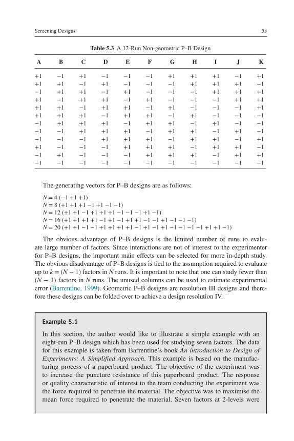
Screening Designs 53
The generating vectors for P–B designs are as follows:
N = 4 (−1 +1 +1)N = 8 (+1 +1 +1 −1 +1 −1 −1)N = 12 (+1 +1 −1 +1 +1 +1 −1 −1 −1 +1 −1)N = 16 (+1 +1 +1 +1 −1 +1 −1 +1 +1 −1 −1 +1 −1 −1 −1)N = 20 (+1 +1 −1 −1 +1 +1 +1 +1 −1 +1 −1 +1 −1 −1 −1 −1 +1 +1 −1)
The obvious advantage of P–B designs is the limited number of runs to evalu-ate large number of factors. Since interactions are not of interest to the experimenter for P–B designs, the important main effects can be selected for more in-depth study. The obvious disadvantage of P–B designs is tied to the assumption required to evaluate up to k = (N − 1) factors in N runs. It is important to note that one can study fewer than (N − 1) factors in N runs. The unused columns can be used to estimate experimental error (Barrentine, 1999). Geometric P–B designs are resolution III designs and there-fore these designs can be folded over to achieve a design resolution IV.
Table 5.3 A 12-Run Non-geometric P–B Design
A B C D E F G H I J K
+1 −1 +1 −1 −1 −1 +1 +1 +1 −1 +1+1 +1 −1 +1 −1 −1 −1 +1 +1 +1 −1−1 +1 +1 −1 +1 −1 −1 −1 +1 +1 +1+1 −1 +1 +1 −1 +1 −1 −1 −1 +1 +1+1 +1 −1 +1 +1 −1 +1 −1 −1 −1 +1+1 +1 +1 −1 +1 +1 −1 +1 −1 −1 −1−1 +1 +1 +1 −1 +1 +1 −1 +1 −1 −1−1 −1 +1 +1 +1 −1 +1 +1 −1 +1 −1−1 −1 −1 +1 +1 +1 −1 +1 +1 −1 +1+1 −1 −1 −1 +1 +1 +1 −1 +1 +1 −1−1 +1 −1 −1 −1 +1 +1 +1 −1 +1 +1−1 −1 −1 −1 −1 −1 −1 −1 −1 −1 −1
Example 5.1
In this section, the author would like to illustrate a simple example with an eight-run P–B design which has been used for studying seven factors. The data for this example is taken from Barrentine’s book An introduction to Design of Experiments: A Simplified Approach. This example is based on the manufac-turing process of a paperboard product. The objective of the experiment was to increase the puncture resistance of this paperboard product. The response or quality characteristic of interest to the team conducting the experiment was the force required to penetrate the material. The objective was to maximise the mean force required to penetrate the material. Seven factors at 2-levels were

Design of Experiments for Engineers and Scientists54
The data was analysed using Minitab software and the results are illustrated below. The first task was to identify the key main effects that were most influential on the response (i.e. force). Figure 5.1 presents a standardised normal plot of effects for the above experiment. Effects C, E and B fall away from the straight line, which implies that they are statistically significant at 5% significance level. Effects A, D, F and G fall along the straight line and therefore can be treated as inactive effects. It is important to note that one can consider even a 10% significance level for screening designs in order to ensure that no important factor effects or parameters are omitted in the first round of experimentation.
In order to substantiate the findings of normal plot, the author have used the Pareto plot of effects. The Pareto plot (Figure 5.2) shows that effects C (press roll
studied using an eight-run geometric P–B design. Table 5.4 presents the factors selected from the brainstorming session and their levels.
Table 5.5 presents the results of an eight-run geometric P–B design experi-ment with two replicates per experimental trial condition.
Table 5.4 List of Factors and Their Levels for the Experiment
Factors Labels Low-Level Setting
High-Level Setting
Paste temperature A 130°F 160°FAmount of additive B 0.2% 0.5%Press roll pressure C 40 psi 80 psiPaper moisture D Low HighPaste type E No clay With clayCure time F 10 days 5 daysMachine speed G 120 fpm 200 fpm
Table 5.5 Design Matrix of an Eight-Run Geometric P–B Design for the Experiment
A B C D E F G R1 R2
+1 −1 −1 +1 −1 +1 +1 12.5 16.84+1 +1 −1 −1 +1 −1 +1 42.44 39.29+1 +1 +1 −1 −1 +1 −1 55.08 47.57−1 +1 +1 +1 −1 −1 +1 49.37 47.69+1 −1 +1 +1 +1 −1 −1 55.43 52.80−1 +1 −1 +1 +1 +1 −1 42.51 35.02−1 −1 +1 −1 +1 +1 +1 51.13 57.92−1 −1 −1 −1 −1 −1 −1 15.61 13.65

Screening Designs 55
pressure), E (paste type) and B (amount of additive) are most important to the pro-cess and therefore should be studied in greater depth. The effect plot of the signifi-cant effects is shown in Figure 5.3.
From the above results, one may conclude that main effects C (press roll pres-sure), E (paste type) and B (amount of additive) are found to have significant impact on the mean puncture resistance (i.e. the force required to penetrate the paper board).
In order to analyse the factors affecting variability in force, we need to calculate the SD of observations at each experimental design point. The results are given in
0 5 10
–1.5
–1.0
–0.5
0.0
0.5
1.0
1.5
Standardised effect
Nor
mal
sco
re
C
E
B
Figure 5.1 NPP of standardised effects.
0 2 4 6 8 10 12 14
Machine speed
Cure time
Paste temperature
Paper moisture
Amount of additive
Paste type
Press roll pressure
Figure 5.2 Pareto plot of the effects for the experiment.

Design of Experiments for Engineers and Scientists56
Table 5.6. As we have seen before in the cake baking example (refer to Chapter 3), the SD of observations do not follow a normal distribution. Therefore we transform the sample SD by taking their logarithms, as the logarithms of the SD will be much closer to being normally distributed (refer to Chapter 3). It is important to note that SD can be computed using any scientific calculator.
Figure 5.4 shows a standardised normal plot of effects affecting ln(SD). The nor-mal plot indicates that only factor F (cure time) influenced the variation in the punc-ture resistance (i.e. force). Further analysis of factor F has revealed that variability is maximum when cure time is set at high level (i.e. 5 days). This can be seen in Figure 5.5.
The conclusions are that factors C, B and E have a significant impact on process average, whereas factor F has a significant impact on process variability. The other
Amount of additive
0.2%
0.5%
40 80 No
clay
With
cla
y
Press roll pressure Paste type
30
35
40
45
50
For
ce
Figure 5.3 Main effects plot of the significant effects.
Table 5.6 Design Matrix of an Eight-Run Geometric P-B Design with Standard Deviation Values
A B C D E F G s ln(SD)
+1 −1 −1 +1 −1 +1 +1 3.07 1.122+1 +1 −1 −1 +1 −1 +1 2.23 0.802+1 +1 +1 −1 −1 +1 −1 5.31 1.670−1 +1 +1 +1 −1 −1 +1 1.18 0.166+1 −1 +1 +1 +1 −1 −1 1.86 0.621−1 +1 −1 +1 +1 +1 −1 5.30 1.668−1 −1 +1 −1 +1 +1 +1 4.80 1.569−1 −1 −1 −1 −1 −1 −1 1.39 0.329
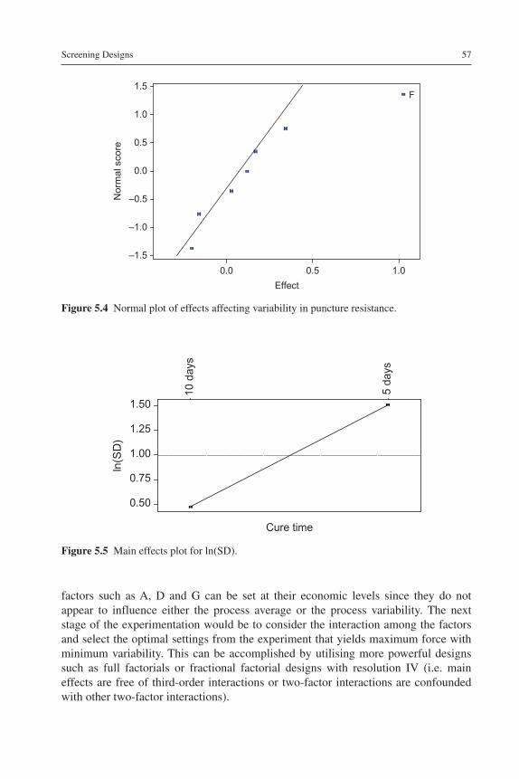
Screening Designs 57
factors such as A, D and G can be set at their economic levels since they do not appear to influence either the process average or the process variability. The next stage of the experimentation would be to consider the interaction among the factors and select the optimal settings from the experiment that yields maximum force with minimum variability. This can be accomplished by utilising more powerful designs such as full factorials or fractional factorial designs with resolution IV (i.e. main effects are free of third-order interactions or two-factor interactions are confounded with other two-factor interactions).
0.0 0.5 1.0
–1.5
–1.0
–0.5
0.0
0.5
1.0
1.5
Effect
Nor
mal
sco
re
F
Figure 5.4 Normal plot of effects affecting variability in puncture resistance.
Cure time
10 d
ays
5 da
ys
0.50
0.75
1.00
1.25
1.50
ln(S
D)
Figure 5.5 Main effects plot for ln(SD).

Design of Experiments for Engineers and Scientists58
Example 5.2
In this example, we consider a plastic foam extrusion process. A process improvement team was formed to investigate what affects the porosity of plastic parts. After a thorough brainstorming session with quality engineers, the process manager and the operators, it was identified that eight process parameters might have some impact on porosity. Table 5.7 presents the list of parameters and their levels for the experiment. Each factor was studied at 2-levels. As the total degrees of freedom for studying eight factors at 2-levels is equal to 8, it was decided to choose a non-geometric 12-run P–B design with 11 degrees of freedom. The extra 3 degrees of freedom can be used to estimate experimental error. Table 5.8 presents the experimental layout with response values in both standard and ran-dom order.
Table 5.8 Experimental Layout for 12-Run P–B Design with Response Values
Run A B C D E F G H Porosity (%)
1 (6) +1 +1 −1 +1 +1 +1 −1 −1 44.8 2 (11) +1 −1 +1 +1 +1 −1 −1 −1 37.2 3 (9) −1 +1 +1 +1 −1 −1 −1 +1 36.0 4 (7) +1 +1 +1 −1 −1 −1 +1 −1 34.8 5 (2) +1 +1 −1 −1 −1 +1 −1 +1 46.4 6 (1) +1 −1 −1 −1 +1 −1 +1 +1 24.8 7 (5) −1 −1 −1 +1 −1 +1 +1 −1 43.6 8 (12) −1 −1 +1 −1 +1 +1 −1 +1 44.8 9 (3) −1 +1 −1 +1 +1 −1 +1 +1 24.010 (8) +1 −1 +1 +1 −1 +1 +1 +1 34.411 (4) −1 +1 +1 −1 +1 +1 +1 −1 27.212 (10) −1 −1 −1 −1 −1 −1 −1 −1 49.6
Note: Numbers in parentheses represent the random order of experimental runs or trials.
Table 5.7 List of Process Parameters and Their Levels for the Experiment
Process Parameters Labels Low Level (−1) High Level (+1)
Temperature profile A 1 2Temperature after heating B 210°C 170°CTemperature after expansion C 170°C 150°CTemperature before coating die D 130°C 115°CExtrusion speed E 6 m/min 4.5 m/minAdhesive coating thickness F 0.7 mm 0.4 mmAdhesive coating temperature G 115°C 100°CExpansion angle H Max Min

Screening Designs 59
Figure 5.6 shows that process parameters such as G (adhesive coating tempera-ture), E (extrusion speed) and F (adhesive coating thickness) have significant impact on porosity. These parameters should be further explored using full fractional designs and more advanced methods such as response surface methods, if necessary. In the next stage of experimentation, one should analyse the interactions among the parameters E, F and G. In order to identify which levels of these parameters yield minimum porosity, we may consider an effects plot (Figure 5.7). Figure 5.7 shows that E at high level, F at low level and G at high level yields minimum porosity.
The objective of the experiment was to determine the key parameters that affect percentage porosity. The Minitab software system was used for analysis purposes. Figure 5.6 illustrates a standardised Pareto plot of effects for the experiment.
543210
G
E
F
H
B
C
D
A
Nor
mal
sco
re
Standardised effect
Figure 5.6 Standardised Pareto plot of Effects for the plastic foam extrusion process.
A B C D
1111 1 1 1 1–1–1–1–1–1 –1 –1 –1
E F G H
32.0
34.5
37.0
39.5
42.0
%po
rosi
ty
Process parameters
Figure 5.7 Main effects plot for the experiment.
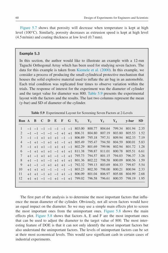
Design of Experiments for Engineers and Scientists60
Example 5.3
In this section, the author would like to illustrate an example with a 12-run Taguchi Orthogonal Array which has been used for studying seven factors. The data for this example is taken from Kiemele et al. (2000). In this example, we consider a process of producing the small cylindrical protective mechanism that houses the solid explosive material used to inflate the air bag in an automobile. Each trial condition was replicated four times to observe variation within the trials. The response of interest for the experiment was the diameter of cylinder and the target value for diameter was 800. Table 5.9 presents the experimental layout with the factors and the results. The last two columns represent the mean (y-bar) and SD of diameter of the cylinder.
Table 5.9 Experimental Layout for Screening Seven Factors at 2-Levels
Run A B C D E F G Y1 Y2 Y3 Y4 y-bar SD
1 −1 −1 −1 −1 −1 −1 −1 803.00 800.77 804.64 799.34 801.94 2.352 −1 −1 −1 −1 −1 +1 +1 806.31 804.80 807.19 803.80 805.53 1.523 −1 −1 +1 +1 +1 −1 −1 806.89 795.18 797.31 809.94 802.33 7.194 −1 +1 −1 +1 +1 −1 +1 805.49 795.47 794.50 804.59 800.01 5.835 −1 +1 +1 −1 +1 +1 −1 802.29 801.69 799.96 802.94 801.72 1.286 −1 +1 +1 +1 −1 +1 +1 811.38 798.87 811.01 800.78 805.51 6.617 +1 −1 +1 +1 −1 −1 +1 795.73 794.57 801.15 794.03 796.37 3.268 +1 −1 +1 −1 +1 +1 +1 801.36 802.22 798.58 800.09 800.56 1.599 +1 −1 −1 +1 +1 +1 −1 792.32 799.13 803.69 804.33 799.87 5.54
10 +1 +1 +1 −1 −1 −1 −1 803.23 802.30 798.00 800.21 800.94 2.3311 +1 +1 −1 +1 −1 +1 −1 806.09 801.04 806.97 805.88 804.99 2.6812 +1 +1 −1 −1 +1 −1 +1 799.02 796.58 796.61 800.55 798.19 1.95
Figure 5.7 shows that porosity will decrease when temperature is kept at high level (100°C). Similarly, porosity decreases as extrusion speed is kept at high level (4.5 m/min) and coating thickness at low level (0.7 mm).
The first part of the analysis is to determine the most important factors that influ-ence the mean diameter of the cylinder. Obviously, not all seven factors would have an equal impact on the diameter. So we may use a simple main effects plot to screen the most important ones from the unimportant ones. Figure 5.8 shows the main effects plot. Figure 5.8 shows that factors A, E and F are the most important ones that can be used to adjust the diameter to the target value of 800. The most inter-esting feature of DOE is that it can not only identify the most important factors but also understand the unimportant factors. The levels of unimportant factors can be set at their most economical levels. This would save significant cash in certain cases of industrial experiments.

Screening Designs 61
The next part of the analysis is to understand the factors which influence vari-ability in diameter. In this instance, it is not only important to achieve a mean diam-eter closer to the target of 800 but also to achieve consistent diameter values closer to 800. In order to analyse variability, we compute SD at each experimental design point and use logarithmic transformation for validating normal distribution assump-tions. This point is very well covered in Lochner and Matar (1990). It was a surprise to observe from Figure 5.9 that factor D is the only factor which causes variation
Mea
n of
mea
ns
21 21 21
21 21 21
21
802.5
801.5
800.5
802.5
801.5
800.5
802.5
801.5
800.5
A B C
D E F
G
Main effects plot (data means) for means
Figure 5.8 Main effects plot for the experiment (mean diameter).
Mea
n of
mea
ns
21 21 21
21 21 21
21
0.6
0.4
0.2
0.6
0.4
0.2
0.6
0.4
0.2
A B C
D E F
G
Main effects plot (data means) for log (SD)
Figure 5.9 Main effects plot for the experiment (analysis of diameter variability).

Design of Experiments for Engineers and Scientists62
in the diameter of the cylinder. Moreover, it points out that minimum variation is obtained when we keep this factor at its low-level setting. This is a very useful piece of information for any designed experiment.
Exercises
1. What are screening designs?2. Compare geometric and non-geometric P–B designs.3. What are the strengths and limitations of P–B designs?4. When would you utilise screening designs in real-life situations?5. Explain how to overcome the problem of low resolution in a screening design.
References
Antony, J., 2002. Training for design of experiments using a catapult. Qual. Reliab. Eng. Int. 18 (1), 29–35.
Barrentine, L.B., 1999. An Introduction to Design of Experiments: A Simplified Approach. ASQ Quality Press, Milwaukee, WI.
Kiemele, M., et al., 2000. Basic Statistics: Tools for Continuous Improvement, fourth ed. Air Academy Press and Associates, Colorado Springs, CO, USA.
Lochner, R.H., Matar, J.E., 1990. Designing for Quality. Productivity Press, USA.Plackett, R.L., Burmann, J.P., 1946. Design of optimal multifactorial experiments. Biometrika
33 (4), 305–325.Wheeler, D.J., 1988. Understanding Industrial Experimentation. Statistical Process Controls,
Inc., Tennessee.

Design of Experiments for Engineers and Scientists. DOI: Copyright © 2014 Jiju Antony. Published by Elsevier Ltd. All rights reserved.
http://dx.doi.org/10.1016/B978-0-08-099417-8.00006-7
Full Factorial Designs6
6.1 Introduction
It is widely accepted that the most commonly used experimental designs in manu-facturing companies are full and fractional factorial designs at 2-levels and 3-levels. Factorial designs would enable an experimenter to study the joint effect of the fac-tors (or process/design parameters) on a response. A factorial design can be either full or fractional factorial. This chapter is primarily focused on full factorial designs at 2-levels only. Factors at 3-levels are beyond the scope of this book. However, if readers wish to learn about experimental design for factors at 3-levels, the author would suggest them to refer to Montgomery (2001).
A full factorial designed experiment consists of all possible combinations of lev-els for all factors. The total number of experiments for studying k factors at 2-levels is 2k. The 2k full factorial design is particularly useful in the early stages of experi-mental work, especially when the number of process parameters or design param-eters (or factors) is less than or equal to 4. One of the assumptions we make for factors at 2-levels is that the response is approximately linear over the range of the factor settings chosen. The first design in the 2k series is one with only two factors, say, A and B, each factor to be studied at 2-levels. This is called a 22 full factorial design.
6.2 Example of a 22 Full Factorial Design
Here we consider a simple nickel plating process with two plating process param-eters: plating time and plating solution temperature (Kiemele et al., 1997). Each pro-cess parameter is studied at 2-levels. The response of interest to the experimenters was plating thickness. Table 6.1 illustrates the two process parameters and their cho-sen levels for the experiment.
Table 6.1 Process Parameters and Their Levels for the Experiment
Process Parameters Labels Low Level High Level
Plating time A 4 s 12 sPlating solution temperature B 16°C 32°C

Design of Experiments for Engineers and Scientists64
Table 6.2 shows the design layout of the experiment with response values. Each experimental condition was replicated five times so that a reasonable estimate of error variance (or experimental error) could be obtained.
The following are the four objectives set by the experimenter:
1. Which main effects or interactions might affect the mean plating thickness?2. Which main effects or interactions might influence variability in plating thickness?3. What is the best setting of factors to minimise variability in thickness?4. How can a target plating thickness of 120 units be achieved?
6.2.1 Objective 1: Determination of Main/Interaction Effects That Influence Mean Plating Thickness
In order to determine the effect of process parameters A and B and its interaction AB, we need to construct a coded design matrix with mean plating thickness values as shown in Table 6.3.
The column AB is obtained by simply multiplying the coded values in columns A and B. Interaction AB yields a combined effect of two factors, A and B. The results from Minitab software are shown below. Figure 6.1 illustrates the normal plot of effects. The graph illustrates that process parameter ‘plating time’ and the interaction between ‘plating time and plating solution temperature’ are statistically significant at 5% significance level. In other words, these effects have a large impact on the mean plating thickness, though plating solution temperature has very little impact on the mean plating thickness. This finding can be further supported by considering the main effects plot and interaction plot (see Figures 6.2 and 6.3, respectively).
It can be seen from Figure 6.2 that plating time has a huge impact on plating thickness, whereas plating solution temperature has no impact on plating thickness
Table 6.2 Design layout of the Experiment with Response Values
Trial Number A B Plating Thickness
1 4 16 116.1 116.9 112.6 118.7 114.92 4 32 106.7 107.5 105.9 107.1 106.53 12 16 116.5 115.5 119.2 114.7 118.34 12 32 123.2 125.1 124.5 124.0 124.7
Table 6.3 Coded Design Matrix with Mean Plating Thickness Values
A B AB Mean Plating Thickness
−1 −1 1 115.84−1 1 −1 106.74
1 −1 −1 116.841 1 1 124.30

0 5 10
–0.5
0.0
0.5
Standardised effect
Nor
mal
sco
re
A
AB
A: Plating timeB: Plating temp.
Figure 6.1 NPP of effects for the plating experiment.
Plating time Plating solution temperature
111.0
113.5
116.0
118.5
121.04 12 16 32
Pla
ting
thic
knes
s
Figure 6.2 Main effects plot for the plating experiment.
412
16 32
108
113
118
123
Plating solution temperature
Plating time
Mea
n pl
atin
g th
ickn
ess
Figure 6.3 Interaction plot – plating time × plating solution temperature.

Design of Experiments for Engineers and Scientists66
whatsoever. However, it is interesting to note that plating solution temperature has a lower sensitivity to variability in plating thickness when compared to plating time. Figure 6.3 indicates that there is a strong interaction between plating time and plat-ing thickness. Plating thickness is maximum when plating time is kept at high level (12 s) and plating solution temperature is kept at high level (32°C). Similarly, plating thickness is minimum when plating solution temperature is kept at high level (32°C) and plating time is kept at low level (4 s).
6.2.2 Objective 2: Determination of Main/Interaction Effects That Influence Variability in Plating Thickness
In order to determine the effect of A, B and interaction AB on process variability, we need to construct a coded design matrix with response as variability in plating thick-ness (Table 6.4).
Minitab software is used to identify which effects are most important to process variability. Figure 6.4 shows a Pareto plot of the effects on variability [ln(SD)]. It is quite clear from the graph that process parameter plating solution temperature (B)
Table 6.4 Coded Design Matrix with Variability as Response
A B AB Variability in Plating Thickness (SD)
ln(SD)
−1 −1 1 2.278 0.823−1 1 −1 0.607 −0.499
1 −1 −1 1.884 0.6331 1 1 0.731 −0.313
0.0 0.5 1.0
A
AB
B
A: Plating timeB: Plating temp.
Figure 6.4 Pareto plot of effects on plating thickness variability.

Full Factorial Designs 67
has a significant effect on plating thickness variability, whereas plating time (A) has no impact on plating thickness variability. Interaction AB has again very little impact on variability. Figure 6.5 shows that variability is minimum when the plating solu-tion temperature is set at high level (32°C). This finding provides the answer to our objective 3, set out earlier in this chapter.
6.2.3 Objective 4: How to Achieve a Target Plating Thickness of 120 Units?
In order to achieve a target plating thickness of 120 units, we need to initially develop a simple regression model (or mathematical model) which connects the response of interest (i.e., plating thickness) and the significant process parameters. In order to develop a regression model, we need to construct a table of effects and regression coefficients (Kiemele et al., 1997). It is important to recall that regression coefficients for factors at 2-levels are just half the estimate of effect. A sample cal-culation of how to estimate the effect of paste time and the interaction between time and temperature is shown below (Table 6.3).
Effect of Plating Time on Plating ThicknessMean plating thickness at high level of plating time = (116.84 + 124.30)/2
= 120.57Mean plating thickness at low level of plating time = (115.84 + 106.74)/2
= 111.29Effect of plating time on plating thickness = (120.57 – 111.29)
= 9.28Regression coefficient of plating time (A) = 9.28/2
= 4.64
Plating time Plating solution temperature
–0.40
–0.15
0.10
0.35
0.60
4 12 16 32
ln(S
D)
Figure 6.5 Main effects plot with variability as response.

Design of Experiments for Engineers and Scientists68
Interaction Effect Between Plating Time and Plating Solution Temperature (AB)
Referring to Column 3 in Table 7.3, the mean plating thickness at low level of AB = (106.74 + 116.84)/2
= 111.79Similarly, the mean plating thickness at high level of AB = (115.84 + 124.30)/2 = 120.07
Therefore, interaction AB = 120.07 – 111.79 = 8.28
Regression coefficient of the interaction term (AB) = 4.14
The regression model for the plating thickness can be therefore written as
ˆ ( ) ( )y A AB= + +β β β0 1 12
where
β0 = overall mean plating thickness = 115.93
β1 = regression coefficient of factor A (plating time)
β12 = regression coefficient of interaction AB (plating time × plating solution temperature)
The predicted model for plating thickness is therefore given by
y = + +115.93 4.64 (A) 4.14 (AB)
Using the above predicted model, we need to determine the settings of parameters which give a target thickness of 120 units (i.e., y = 120). Moreover, we know that a high level of plating solution temperature (factor B) yields minimum variability. Therefore, we can set B at a low level (i.e., 1).
Now, we can write, 120 = 115.93 + 4.64 (A) + 4.14 (A) = 115.93 + 4.64 A + 4.14 A = 115.93 + 8.78 A
4.07 = 8.78 AA = 0.463 (in coded terms)
= 8.28 = 8.28 = 8.28 = 8.28The following equation can be used to convert the coded values into actual
parameter values (or vice versa).
ActualHigh Low High Low
Coded=+
+
−
•
2 2
For example, for factor A, high-level setting = 12 s, low-level setting = 4 s, coded value = 0.463:Actual = {(12 + 4)/2} + {((12 – 4)/2)) . 0.463}
= 8 + 4 (0.463) = 9.85 sec
(6.1)
(6.2)

Full Factorial Designs 69
Therefore, to achieve a target plate thickness of 120 units, we need to set the plat-ing time for 9.85 s at a temperature of 32°C. We need to perform confirmation exper-iments or runs to verify the results of our analysis. If the results of the confirmation experiments or runs (i.e., each observation from the trials) fall within the interval of y � 3 (s.e.), then the results are satisfactory. Here s.e. refers to standard error and is
obtained by s n/ , where SD is the sample standard deviation and n is sample size.
The analysis of a 2k factorial design assumes that the observations are normally and independently distributed (Logothetis, 1992). The best way to check the normal-ity assumption is by constructing an NPP of residuals (Box et al., 1978). Figure 6.6 presents the normal probability of residuals for the plating experiment. As the residu-als fall approximately along a straight line, we can conclude that the data come from a normal population.
6.3 Example of a 23 Full Factorial Design
Now we consider an experiment with three factors at 2-levels. The response of inter-est for the experiment was yield of a chemical process. The list of process param-eters and their levels are presented in Table 6.5.
It was important to analyse all the two-factor interactions and therefore a 23 full factorial design was chosen. Each trial condition was replicated three times in order
–3 –2 –1 0 1 2 3
–2
–1
0
1
2
Nor
mal
sco
re
Residual
Figure 6.6 NPP of residuals for the plating experiment.
Table 6.5 List of Process Parameters and Their Levels
Process Parameters Labels Low Level High Level
Temperature T 80°C 120°CPressure P 50 psi 70 psiReaction time R 5 min 15 min

Design of Experiments for Engineers and Scientists70
to obtain an accurate estimate of experimental error (or error variance). The follow-ing objectives were set prior to performing the experiment.
1. Which main effects or interactions might affect the average process yield?2. Which main effects or interactions might influence variability in process yield?3. What is the optimal process condition?
6.3.1 Objective 1: To Identify the Significant Main/Interaction Effects That Affect the Process Yield
In order to identify the significant main/interaction effects, it was decided to con-struct an experimental layout (Table 6.6), which shows all the combinations of process parameters at their respective levels. The table shows the actual settings of the process parameters with the response values (i.e., yield) recorded at each trial condition.
Figure 6.7 illustrates the Pareto plot of effects. The graph shows that main effects T (temperature) and R (reaction time), and interaction between pressure (P) and reaction time (R), are significant at 5% significance level. It is quite interesting to note that pressure (P) on its own has no significant impact on the process yield. It is important to analyse the interaction between P and R for determining the best set-tings for optimising the chemical process yield.
Figure 6.8 indicates that there exists a strong interaction between pressure and reaction time. It is clear that the effects of reaction time at different levels of pressure are different. Yield is minimum when the pressure is kept at a low level (50 psi) and reaction time at high level (15 min). Maximum yield is obtained when the pressure and reaction time are kept at low levels.
6.3.2 Objective 2: To Identify the Significant Main/Interaction Effects That Affect the Variability in Process Yield
In order to identify the significant main/interaction effects that affect process vari-ability, we need to construct a coded design matrix with ln(SD) as the response of interest. Table 6.7 illustrates the design matrix with variability as the response.
Table 6.6 Experimental Layout with Response Values
Run/trial T P R Yield 1 (%) Yield 2 (%) Yield 3 (%)
1 80 50 5 61.43 58.58 57.072 120 50 5 75.62 77.57 75.753 80 70 5 27.51 34.03 25.074 120 70 5 51.37 48.49 54.375 80 50 15 24.80 20.69 15.416 120 50 15 43.58 44.31 36.997 80 70 15 45.20 49.53 50.298 120 70 15 70.51 74.00 74.68

Full Factorial Designs 71
20100
PR
T
R
TP
TR
P
TPR
T: TemperatureP: PressureR: Reaction time
Figure 6.7 Pareto plot of effects for the yield example.
5070
5 15
35
45
55
65
Reaction time
Pressure
Ave
rage
yie
ld
Figure 6.8 Interaction plot – pressure × reaction time.
Table 6.7 Design Matrix with Variability as Response of Interest
Run T P R SD ln(SD)
1 −1 −1 −1 2.214 0.7952 1 −1 −1 1.090 0.0863 −1 1 −1 4.632 1.5334 1 1 −1 2.940 1.0785 −1 −1 1 4.707 1.5496 1 −1 1 4.032 1.3947 −1 1 1 2.746 1.0108 1 1 1 2.237 0.805

Design of Experiments for Engineers and Scientists72
Due to zero degrees of freedom for the error term, we need to rely on a procedure called ‘pooling’ of insignificant effects (Taguchi, 1987). Pooling is a process of obtaining a more accurate estimate of error variance. Taguchi advocates pooling effects until the degrees of freedom for the error term is approximately equal to half the total degrees of freedom for the experiment.
For the present example, the author has pooled interactions TR, TP and TPR so that three degrees of freedom have been created for the error term. A Pareto plot of the effects is shown in Figure 6.9. The figure shows that none of the main effects have any impact on variability. Interaction between pressure (P) and reaction time (R) seems to have some impact on variability (Figure 6.10). It can be seen that vari-ability is minimum when pressure is kept at low level and reaction time at low level.
543210
PR
T
R
P
T: Temperature
P: Pressure
R: Reaction time
Figure 6.9 Pareto plot of effects with ln(SD) as response of interest.
5070
5 15
0.50.60.70.80.91.01.11.21.31.4
Reaction time
PressureMea
n ln
(SD
)
Figure 6.10 Interaction plot of ln(SD) – pressure × reaction time.

Full Factorial Designs 73
6.3.3 Objective 3: What Is the Optimal Process Condition?
In order to determine the optimal condition for the process, it is important that we need to analyse both response mean and variability. The best settings for maximising the process yield are as follows:
Temperature (T) – High level (120°C)Pressure (P) – Low level (50 psi)Reaction time (R) – Low level (5 min)
Similarly, the best settings for minimising response variability are:
Temperature (T) – High level (120°C)Pressure (P) – Low level (50 psi)Reaction time (R) – Low level (5 min)
The above settings can be easily obtained by analysing the mean process yield and mean ln(SD) values at both low- and high-level settings of T, P and R.
For normality assumption of data, it is best to construct an NPP of residuals (Figure 6.11). The graph indicates that the data come from a normal population.
6.4 Example of a 24 Full Factorial Design
In the last example, the author will consider an example with four factors. This example shows the results of an experiment to study the effect of four factors on a cracking problem. A nickel–titanium alloy is used to make components for jet turbine aircraft engines. Cracking is a potentially serious problem in the final part, because it can lead to non-recoverable failure and subsequent rejection of the part, thereby causing waste. The objective of the experiment was therefore to identify the key factors and their interactions (if existing) which have effect on cracks. Four factors were considered: (pouring temperature (A), titanium content (B), heat treat-ment method (C) and the amount of grain refiner used (D). Each factor was studied
–5 0 5
–2
–1
0
1
2
Nor
mal
sco
re
Residual
Figure 6.11 NPP of residuals for the yield experiment.

Design of Experiments for Engineers and Scientists74
at 2-levels and a 24 full factorial design was selected. Table 6.8 presents the experi-mental layout used for this experiment to minimise cracks. The response of interest to the experimenter was the length of crack (in mm × 10−2). Each trial condition was replicated twice to estimate error variance.
The following are the objectives of the experiment:
1. Which of the main/interaction effects affect mean crack length?2. Which main effects or interactions might influence variability in crack length?3. What is the optimal process condition to minimise mean crack length?
6.4.1 Objective 1: Which of the Main/Interaction Effects Affect Mean Crack Length?
In order to identify the key main and interaction effects that affect crack length, a Pareto plot of effects (Figure 6.12) was constructed. The Pareto plot clearly indicates that all the main effects (A, B, C and D) and two two-factor interactions (AB and AC) are statistically significant at 5% significance level. In order to understand the nature of interactions among the factors, the author would suggest that readers refer to Figure 6.13.
Figure 6.13 indicates that there is a strong interaction between A and B; and A and C (due to non-parallel lines). We don’t generally study three-factor (or three-way) interactions as they are not important in real-life settings.
Table 6.8 Experimental Layout with Response Values
Run A B C D Crack Length
1 −1 −1 −1 −1 7.037 6.3762 1 −1 −1 −1 14.707 15.2193 −1 1 −1 −1 11.635 12.0894 1 1 −1 −1 17.273 17.8155 −1 −1 1 −1 10.403 10.1516 1 −1 1 −1 4.368 4.0987 −1 1 1 −1 9.360 9.2538 1 1 1 −1 13.440 12.9239 −1 −1 −1 1 8.561 8.951
10 1 −1 −1 1 16.867 17.05211 −1 1 −1 1 13.876 13.65812 1 1 −1 1 19.824 19.63913 −1 −1 1 1 11.846 12.33714 1 −1 1 1 6.125 5.90415 −1 1 1 1 11.190 10.93516 1 1 1 1 15.653 15.053

Full Factorial Designs 75
6.4.2 Objective 2: Which of the Main/Interaction Effects Affect Variability in Crack Length?
For many industrial experiments, it is important to understand which factors affect mean response and which ones affect response variability. For optimisation prob-lems, we need to minimise response variability around the target performance (Dean and Voss, 1999). This is one of the fundamental objectives of robust design methodology.
0 1 2 3 4 5
BD
AD
CD
BC
AB
D
A
C
B
AC
A: AB: BC: CD: D
Figure 6.12 Pareto plot of effects for the above example.
8
13
188
13
188
13
18A
B
C
D
–11
–1 –11 1 1–1
–11
–11
Figure 6.13 Interactions graph for the experiment.

Design of Experiments for Engineers and Scientists76
In order to analyse which factors affect variability in crack length, we need to construct a design matrix with ln(SD) as the response. Table 6.9 presents the design matrix with ln(SD) as the response of interest.
In order to identify the factors/interactions that affect variability in crack length, a Pareto plot of effects was constructed (Figure 6.14). The Pareto plot has shown that none of the main effects has a significant effect on variability in crack length.
Table 6.9 Experimental Layout with Response Values
Run A B C D SD ln(SD)
1 −1 −1 −1 −1 0.467 −0.7612 1 −1 −1 −1 0.362 −1.0163 −1 1 −1 −1 0.321 −1.1364 1 1 −1 −1 0.383 −0.9605 −1 −1 1 −1 0.178 −1.7266 1 −1 1 −1 0.191 −1.6557 −1 1 1 −1 0.076 −2.5778 1 1 1 −1 0.366 −1.0059 −1 −1 −1 1 0.276 −1.287
10 1 −1 −1 1 0.131 −2.03311 −1 1 −1 1 0.154 −1.87112 1 1 −1 1 0.131 −2.03313 −1 −1 1 1 0.347 −1.05814 1 −1 1 1 0.156 −1.85815 −1 1 1 1 0.180 −1.71516 1 1 1 1 0.424 −0.858
0 1 2 3 4
BD
A
B
BC
C
D
AD
AC
AB
CD
A: AB: BC: CD: D
Figure 6.14 Pareto plot for ln(SD).

Full Factorial Designs 77
Two interactions (AB and CD) are believed to have significant impact on the vari-ability. Figure 6.15 illustrates the interaction plot between factors A and B. It is quite clear from the graph that there exists a strong interaction between factors A and B. The variability in crack length is minimum when A is kept at low level and B at high level. Similarly, C at low level and D at high level yield minimum variability in crack length. However, it is interesting to observe that factor D is less sensitive to variabil-ity when C is kept at high level.
6.4.3 Objective 3: What Is the Optimal Process Condition to Minimise Mean Crack Length?
In this section, the author will demonstrate how to determine the settings of A, B, C and D to minimise mean crack length. As interactions AB and AC have a signifi-cant impact on mean crack length, we need to analyse the mean crack length for all the four combinations between these two factors. Tables 6.10 and 6.11 present the mean crack length at all combinations of factor levels of A and B and A and C, respectively.
1–1
–1 1
–1.8
–1.7
–1.6
–1.5
–1.4
–1.3
–1.2
B
A
Mea
n ln
(SD
)
Figure 6.15 Interaction between A and B (response: ln(SD)).
Table 6.10 Mean Crack Length for All Combinations of A and B
A B Mean Crack Length
−1 −1 9.4581 −1 10.542
−1 1 11.51 1 16.453

Design of Experiments for Engineers and Scientists78
It is also observed that factor D at low level yields minimum crack length. Therefore, the optimal condition of the process to minimise crack length is as follows:
Factor A – Low level (−1)Factor B – Low level (−1)Factor C – High level (1)Factor D – Low level (−1)
The NPP of residuals (Figure 6.16) shows that the data comes from a normal population.
6.4.4 More Examples of FFEs
In this section, we consider a couple of examples to help you understand the use of FFEs in two different contexts. The first example is about obtaining more uniform fill heights in soft drink bottles. The filling machine theoretically fills each bottle to the correct target height. However, the bottle manufacturer was experiencing vari-ation in fill heights and it was quite important for the company to reduce variation around the target height. The engineering team of the company identified three pro-cess variables that could influence the fill heights during the filling process. It was
Table 6.11 Mean Crack Length for All Combinations of A and C
A C Mean Crack Length
−1 −1 10.2731 −1 17.300
−1 1 10.6841 1 9.696
–0.4 –0.3 –0.2 –0.1 0.0 0.1 0.2 0.3 0.4
–2
–1
0
1
2
Nor
mal
sco
re
Residual
Figure 6.16 NPP of residuals for the above data.

Full Factorial Designs 79
decided to keep each process variable at 2-levels. This would lead to eight experi-mental trials or runs. Table 6.12 presents the list of process variables (or factors) and their respective levels for the experiment.
Table 6.13 shows the experimental layout with the list of process variables and the possible combinations.
The response or quality characteristic of interest for the experiment was deviation from the target fill height. Table 6.14 presents the coded layout with the response values.
Table 6.12 List of Process Variables and Their Levels for the Experiment
Process Variables Labels Low Level High Level
Carbonation A 10% 12%Operating pressure B 25 psi 30 psiLine speed C 200 bottles per minute (bpm) 250 bottles per minute (bpm)
Table 6.13 Experimental Layout with All the Process Variables
Experimental Run
A (%) B C
1 10 25 2002 12 25 2003 10 30 2004 12 30 2005 10 25 2506 12 25 2507 10 30 2508 12 30 250
Table 6.14 Coded Experimental Layout with Response Values
Experimental Run
A B C Deviation from the Target Fill Height (y)
1 −1 −1 −1 −42 +1 −1 −1 13 −1 +1 −1 −14 +1 +1 −1 55 −1 −1 +1 −16 +1 −1 +1 37 −1 +1 +1 28 +1 +1 +1 11

Design of Experiments for Engineers and Scientists80
Figure 6.17 shows a main effects plot for the process variables. The main effects plot shows that carbonation is the most important factor, followed by operating pres-sure and finally line speed. We also look at the interaction graph to determine if any interaction exists among these process variables. Figure 6.18 shows the interac-tion graph for all three process variables. It was found that there is no interaction between carbonation and line speed. However, there was some interaction between the operating pressure and carbonation as well as operating pressure and line speed (Oehlert, 2000).
The second example describes a designed experiment executed to study the influence of four factors on the filtration rate of a high-pressure chemical reactor. Table 6.15 presents the list of factors and levels for the chemical reactor experiment.
The response of interest in this experiment was filtration rate measured in gallons per hour. The objective of the experiment was to understand which factors and their
Mea
n 1210
4.5
3.0
1.5
0.0
3025
250200
4.5
3.0
1.5
0.0
Carbonation Operating pressure
Line speed
Main effects plot for deviation from targetData means
Figure 6.17 Main effects for the process variables.
3025 250200
8
4
0
8
4
0
Carbonation
Operating pressure
Line speed
1012
Carbonation
2530
Operatingpressure
Interaction plot for deviation from targetData means
Figure 6.18 Interaction plot (carbonation, operating pressure and line speed).

Full Factorial Designs 81
interactions (if any) are influencing the response. We also needed to maximise the filtration rate. In other words, we needed to determine the levels of factors that max-imise the filtration rate.
It was decided to perform a 24 FFE with no replicates. Table 6.16 illustrates the results of the 16-run experiment. The table is a coded design matrix showing all the possible combinations of factors at their respective levels. Table 6.16 shows that trial number or run number 12 has provided the experimenters with the highest filtration rate. The lowest filtration is obtained for trial number 9. Having collected the data, the next step was to understand which factors and their interactions have an impact on the filtration rate.
Figure 6.19 shows the main effects plot for the reactor experiment. The main effects plot indicates that temperature and stir rate are the most influential factors,
Table 6.15 Factors and Their Levels for the Reactor Experiment
Factors Labels Units Low Level (−1) High Level (+)
Temperature A °C 24 35Pressure B psig 10 15Concentration C % 2 4Stir rate D rpm 15 30
Table 6.16 Experimental Design Layout with the Results for Reactor Study
Trials A B C D Filtration Rate (Gallons per Hour)
1 −1 −1 −1 −1 45.02 +1 −1 −1 −1 71.03 −1 +1 −1 −1 48.04 +1 +1 −1 −1 65.05 −1 −1 +1 −1 68.06 +1 −1 +1 −1 60.07 −1 +1 +1 −1 80.08 +1 +1 +1 −1 65.09 −1 −1 −1 +1 43.0
10 +1 −1 −1 +1 100.011 −1 +1 −1 +1 45.012 +1 +1 −1 +1 104.013 −1 −1 +1 +1 75.014 +1 −1 +1 +1 86.015 −1 +1 +1 +1 70.016 +1 +1 +1 +1 96.0
Source: Data from Montgomery (2001).

Design of Experiments for Engineers and Scientists82
followed by concentration of formaldehyde and pressure. It was interesting to note that pressure has very little influence on the filtration rate and the level of pressure can be kept at either 10 or 15 psig. The experimenters also wanted to minimise the concentration of formaldehyde and hence we needed to determine the best level of this factor to give the maximum infiltration rate. As this factor did not appear to be the most important factor, and moreover since trials 10 and 12 gave the highest filtra-tion rates at low levels of concentration, we could safely keep this factor at a low-level setting (that is, 2% concentration of formaldehyde). The best possible settings for maximising the filtration rate, therefore, are as follows (based on main effects plot):
Temperature – High level – 35°CPressure – High level – 15 psigConcentration of formaldehyde – Low level – 2%Stir rate – High level – 30 rpm
We also explored the nature of interactions among the factors to make sure that levels were chosen correctly for maximising the filtration rate. Figure 6.20 depicts the interaction plot among all the factors. It is clear from the interaction graph that there are some strong interactions between temperature and concentration of for-maldehyde as well as temperature and stir rate. However, there was no interaction between temperature and pressure, pressure and stir rate or stir rate and concentra-tion of formaldehyde. Further analysis of the interaction graph between temperature and concentration reveals that the filtration rate is highest when temperature is kept at high level and concentration at low level. Also, the interaction graph between tem-perature and stir rate clearly indicates that the filtration rate is maximum when tem-perature and stir rate are kept at high levels.
3524 1510
42
80
75
70
65
60
80
75
70
65
60
3015
TemperatureM
ean
Pressure
Concentration of formaldehyde Stir rate
Main effects plot for filtration rateData means
Figure 6.19 Main effects plot for the reactor experiment.

Full Factorial Designs 83
Exercises
1. An engineer is interested in the effects of cutting speed (CS), tool geometry (TG), and cut-ting angle (CA) on the life (in hours) of a machine tool. A 23 full factorial design was cho-sen and the results are shown below. Each trial condition was replicated twice.
Run CS TG CA Life
1 −1 −1 −1 22 312 1 −1 −1 32 433 −1 1 −1 35 344 1 1 −1 55 475 −1 −1 1 44 456 1 −1 1 40 377 −1 1 1 60 508 1 1 1 39 41
(a) Which effects appear to have a significant effect on the tool life?(b) What is the optimal condition if the objective of the experiment is to maximise tool life?(c) How do you validate the assumption of normality?
2. In a certain casting process for manufacturing jet engine turbine blades, the objective of the experiment is to determine the most significant main and interaction effects that affect part shrinkage. Three factors (mould temperature (A), metal temperature (B) and pour speed (C) were studied at 2-levels using a 23 FFE. The following table presents the results of the experiment. Each trial condition was replicated three times to obtain sufficient degrees of freedom for the error term.
10 42 3015
75
50100
75
50
75
15100
100
50
Temperature
Pressure
Concentration of formaldehyde
Stir rate
2435
Temperature
1015
Pressure
24
Concentration of formaldehyde
Interaction plot for filtration rate
Data means
Figure 6.20 Interaction plot for the reactor experiment.

Design of Experiments for Engineers and Scientists84
Run C B A Shrinkage Values (%)
1 −1 −1 −1 2.22 2.11 2.142 1 −1 −1 1.42 1.54 1.053 −1 1 −1 2.25 2.31 2.214 1 1 −1 1.00 1.38 1.195 −1 −1 1 1.73 1.86 1.796 1 −1 1 2.71 2.45 2.467 −1 1 1 1.84 1.76 1.708 1 1 1 2.27 2.69 2.71
(a) Which effects appear to have a significant effect on the percentage of shrinkage?(b) Which effects appear to have a significant effect on variability in shrinkage?
3. A 23 FFE was conducted to study the influence of temperature (A), pressure (B) and cycle time (C) on the occurrence of splay in an injection moulding process. For each of the eight unique trials, 50 parts were made and the response of interest to the experimenter was the number of incidences of the occurrence of splay on the surface of the part across all 50 parts. The following table shows the experimental layout with the data.
Run A B C Response
1 −1 −1 −1 122 1 −1 −1 153 −1 1 −1 244 1 1 −1 175 −1 −1 1 246 1 −1 1 167 −1 1 1 248 1 1 1 28
(a) Compute all the main and interaction effects.(b) Construct a Pareto plot of the effect estimates. Which of the effects appear to be statisti-
cally significant?
4. A 23 FFE was performed in a packaging industry offering food service products, consumer packaging and packaging machinery. The following table shows the results of the experi-ment with dry crush being the response of the experiment. It was decided to keep the belt tension constant throughout the experiment. Moreover, each trial or run was replicated to capture variability due to process, machine set-up, operator, etc.
(a) Which effects appear to have a significant influence on dry crush?(b) Construct an interaction graph and identify which of the effects interact.

Full Factorial Designs 85
Run Score Depth Speed Temperature Dry Crush
1 High 18 75 311.52 Low 18 75 315.13 High 22 75 261.64 Low 22 75 353.85 High 18 145 280.66 Low 18 145 335.27 High 22 145 353.28 Low 22 145 352.49 High 18 75 299.5
10 Low 18 75 295.111 High 22 75 286.412 Low 22 75 319.013 High 18 145 271.214 Low 18 145 329.415 High 22 145 312.416 Low 22 145 365.6
References
Box, G.E.P., Hunter, W.G., Hunter, J.S., 1978. Statistics for Experimenters. John Wiley, New York, NY.
Dean, A., Voss, D.T., 1999. Design and Analysis of Experiments. Springer Verlag, New York, NY.
Logothetis, N., 1992. Managing for Total Quality. Prentice Hall, UK.Kiemele, M.J., Schmidt, S.R., Berdine, R.J., 1997. Basic Statistics: Tools for Continuous
Improvement, fourth ed. Air Academy Associates, Colorado Springs, CO.Montgomery, D.C., 2001. Design and Analysis of Experiments, fifth ed. John Wiley & Sons,
New York, NY.Oehlert, G.W., 2000. A First Course in Design and Analysis of Experiments. W. H. Freeman &
Co., New York, NY.Taguchi, G., 1987. System of Experimental Design. UNIPUB/Kraus International Publication,
New York, NY.

Design of Experiments for Engineers and Scientists. DOI: Copyright © 2014 Jiju Antony. Published by Elsevier Ltd. All rights reserved.2014
http://dx.doi.org/10.1016/B978-0-08-099417-8.00007-9
Fractional Factorial Designs7
7.1 Introduction
Very often experimenters do not have adequate time, resources or budget to carry out FFEs. If the experimenters can reasonably assume that certain higher-order interac-tions (third order and higher) are not important, then information on the main effects and two-order interactions can be obtained by running only a fraction of the FFE. A type of orthogonal array design which allows experimenters to study main effects and desired interaction effects in a minimum number of trials or experimental runs is called a fractional factorial design. These fractional factorial designs are the most widely and commonly used types of design in industry. These designs are generally represented in the form 2(k−p), where k is the number of factors and 1/2p represents the fraction of the full factorial 2k (Box et al., 1978). For example, 2(5−2) is a 1/4th fraction of a 25 FFE. This means that one may be able to study 5 factors at 2-levels in just 8 experimental trials instead of 32 trials.
7.2 Construction of Half-Fractional Factorial Designs
The construction of half-fractions of a FFE is simple and straightforward. Consider a simple experiment with three factors. Table 7.1 presents the design matrix with all the main and interaction effects assigned to various columns of the matrix. Based on our assumption about three-factor (or third-order) and higher-order interactions being negligible, one could use the ABC interaction column in Table 7.1 to generate settings for the fourth factor D. In other words, we would be able to study four fac-tors using eight runs by deliberately aliasing factor D with ABC interaction. This is referred to as a 2(4−1) factorial design (Table 7.2).
In Table 7.2, D = ABC implies that main effect D is confounded (or aliased) with a third-order interaction ABC. However, a third-order interaction is of no interest to experimenters. The “design generator” of this design is given by D = ABC. We refer to design generator as a word. The defining relation of this design is given by D. D = D2 = ABCD = I, where ‘I’ is the identity element. Once we know the defining relation of a design, we can then generate the alias structure for that particular design.
In the above experiment, I = ABCD (defining relation)In order to determine the alias of A, we multiply both sides of the defining rela-
tion by ‘A’. This yields the following:
A I A A ABCD A BCD BCD as A22 1, .

Design of Experiments for Engineers and Scientists88
We can now generate aliases of B and C as follows:
B I B ACD
C I C ABD
Because we are generally interested in two-factor interactions, we can also gener-ate aliases for all two-factor interactions as follows:
I AB A B CD CD
I AC A C BD BD
I BC B C AD AD
I AD A D CB BC
I
2 2
2 2
2 2
2 2
BBD B D CA AC
I CD C D AB AB
2 2
2 2
Table 7.1 Design Matrix of an Eight-Run Experiment with Three Factors
Run A B AB C AC BC ABC
1 −1 −1 1 −1 1 1 −12 1 −1 −1 −1 −1 1 13 −1 1 −1 −1 1 −1 14 1 1 1 −1 −1 −1 −15 −1 −1 1 1 −1 −1 16 1 −1 −1 1 1 −1 −17 −1 1 −1 1 −1 1 −18 1 1 1 1 1 1 1
Table 7.2 Design Matrix of a 2(4−1) Factorial Design
Run A B AB C AC BC D = ABC
1 −1 −1 1 −1 1 1 −12 1 −1 −1 −1 −1 1 13 −1 1 −1 −1 1 −1 14 1 1 1 −1 −1 −1 −15 −1 −1 1 1 −1 −1 16 1 −1 −1 1 1 −1 −17 −1 1 −1 1 −1 1 −18 1 1 1 1 1 1 1
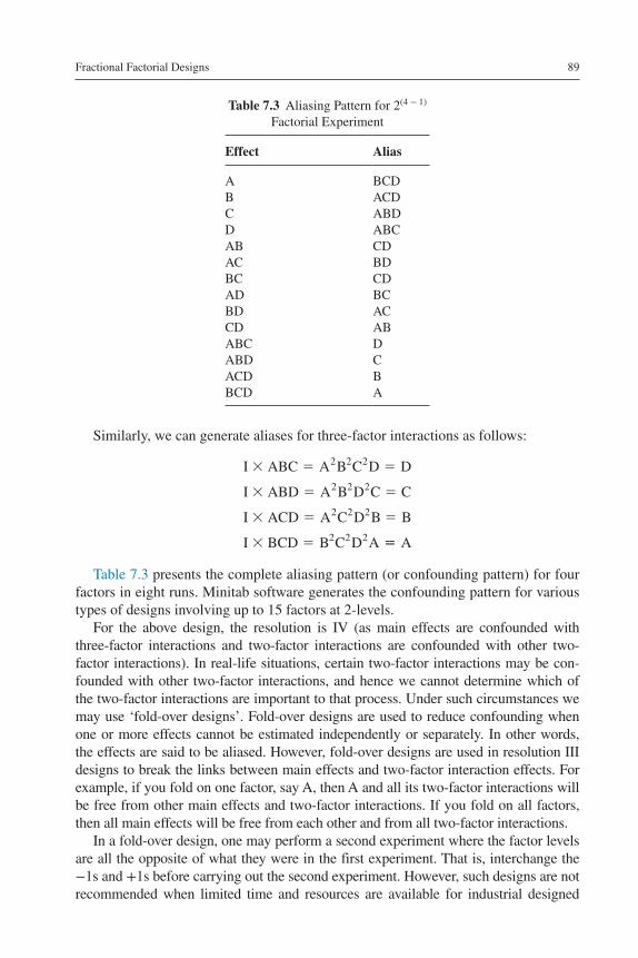
Fractional Factorial Designs 89
Similarly, we can generate aliases for three-factor interactions as follows:
I ABC A B C D D
I ABD A B D C C
I ACD A C D B B
I BCD B C D A
2
2 2 2
2 2
2 2 2
2 2 2 A
Table 7.3 presents the complete aliasing pattern (or confounding pattern) for four factors in eight runs. Minitab software generates the confounding pattern for various types of designs involving up to 15 factors at 2-levels.
For the above design, the resolution is IV (as main effects are confounded with three-factor interactions and two-factor interactions are confounded with other two-factor interactions). In real-life situations, certain two-factor interactions may be con-founded with other two-factor interactions, and hence we cannot determine which of the two-factor interactions are important to that process. Under such circumstances we may use ‘fold-over designs’. Fold-over designs are used to reduce confounding when one or more effects cannot be estimated independently or separately. In other words, the effects are said to be aliased. However, fold-over designs are used in resolution III designs to break the links between main effects and two-factor interaction effects. For example, if you fold on one factor, say A, then A and all its two-factor interactions will be free from other main effects and two-factor interactions. If you fold on all factors, then all main effects will be free from each other and from all two-factor interactions.
In a fold-over design, one may perform a second experiment where the factor levels are all the opposite of what they were in the first experiment. That is, interchange the −1s and +1s before carrying out the second experiment. However, such designs are not recommended when limited time and resources are available for industrial designed
Table 7.3 Aliasing Pattern for 2(4 − 1) Factorial Experiment
Effect Alias
A BCDB ACDC ABDD ABCAB CDAC BDBC CDAD BCBD ACCD ABABC DABD CACD BBCD A

Design of Experiments for Engineers and Scientists90
experiments. Under such circumstances, sound engineering judgements coupled with knowledge in the subject matter would be of great help to experimenters in separating out the main effects from confounded interaction effects.
7.3 Example of a 2(7−4) Factorial Design
The following section describes an example of a fractional factorial design with res-olution III. The example is adapted from Box et al. (1978). This example involves an experiment to study the effect of seven factors at 2-levels using eight trials. The response of interest for the experiment was the time (seconds) taken to climb a hill for a particular person on a bicycle. Table 7.4 illustrates the list of factors and their levels used for the experiment.
Table 7.5 presents the experimental layout with the response values. The runs were performed in random order on eight successive days. This is a 2(7 − 4) factorial design with a design resolution III (i.e. main effects are confounded with two-factor interactions).
Minitab software is used for the statistical analysis of data. The first step in the analy-sis is to identify the most important factors which influence the time to cycle up the hill (seconds). A Pareto plot is constructed to identify the key factors (Figure 7.1). The graph shows that the positions of the gear (D) and the dynamo (B) have a significant effect on the time.
Table 7.4 List of Factors and Their Levels for the Experiment
Factors Labels Low Level High Level
Seat A Up DownDynamo B Off OnHandlebars C Up DownGear D Low MediumRaincoat E On OffBreakfast F Yes NoTyres G Hard Soft
Table 7.5 Experimental Design Layout of the Experiment
Run A B C D = AB E = AC F = BC G = ABC Time to Climb Hill (s)
1 −1 −1 −1 1 1 1 −1 692 1 −1 −1 −1 −1 1 1 523 −1 1 −1 −1 1 −1 1 604 1 1 −1 1 −1 −1 −1 835 −1 −1 1 1 −1 −1 1 716 1 −1 1 −1 1 −1 −1 507 −1 1 1 −1 −1 1 −1 598 1 1 1 1 1 1 1 88

Fractional Factorial Designs 91
The design generators of the above design are as follows:
D AB, E AC, F BC and G ABC� � � �
Therefore defining relation can be obtained as follows:
I ABD ACE BCF ABCG BCDE ACDF ABEFCDG BEG AFG DEF ADEG BDF
� � � � � � �� � � � � � GG ABCDEFG�
As we are interested in only main effects and two-factor interactions, the seven main effects and their aliases can be generated in the following manner. As all fac-tors were studied at 2-levels, we estimate only the linear effects of the factors which are confounded with two-factor interactions. For instance, the linear effect of A (ℓA) is estimated to be 3.5. However, factor A is confounded with three two-factor inter-actions such as BD, CE and FG.
����
A
C
D
A BD CE FGB AD CF EG
C AE BF DG
3 512 01 022
..
..
→→→
B
550 501 02 5
→→→→
D AB CG EFE AC BG DF
F AG BC DEG A
E
F
G
���
... FF BE CD
As only B and D are two significant effects, we need to analyse them further as D is confounded with B and A, and B is confounded with A and D. Here the largest effect is due to factor D and it is not easy to conclude that the effect of D is large just because of factor D or the confounded two-factor interactions. This problem can be tackled by
0 10 20
Raincoat
Breakfast
Handlebars
Tyres
Seat
Dynamo
Gear
Figure 7.1 Pareto plot of effects for the bicycle data.

Design of Experiments for Engineers and Scientists92
folding on factor D and by reversing the signs of column containing factor D. This fold-over design is given in Table 7.6 along with the observed responses. It is quite interest-ing to observe that both factors B and D turn out to be significant again (Figure 7.2).
The effects estimated by the second fraction are as follows:
���
A*
B*
C*
A BD CE FG
B AD CF EG
C AE BF D
0 750
10 25
2 75
.
.
.
→→→ GG
D AB CG EF
E AC BG DF
F AG B
D*
E*
F*
���
25 25
1 75
2 25
.
.
.
→→→ CC DE
G AF BE CDG*� 0 75. →
Table 7.6 Fold-Over Design by Folding on Just One Factor
Run A B C D = −AB E = AC F = BC G = ABC Time to Climb Hill (s)
1 −1 −1 −1 −1 1 1 −1 472 1 −1 −1 1 −1 1 1 743 −1 1 −1 1 1 −1 1 844 1 1 −1 −1 −1 −1 −1 625 −1 −1 1 −1 −1 −1 1 536 1 −1 1 1 1 −1 −1 787 −1 1 1 1 −1 1 −1 878 1 1 1 −1 1 1 1 60
0 5 10 15 20 25
Seat
Tyres
Raincoat
Breakfast
Handlebars
Dynamo
Gear
Figure 7.2 Pareto plot of effects for the fold-over design data.

Fractional Factorial Designs 93
By combining the effect estimates from this second fraction with the effect esti-mates from the original eight runs, we obtain the following estimates of the effects:
� � � �A A A* A*A CE FG or A CE FG21
2( ) ( )
i.e. (3.5 0.750) 2.125 A CE FG
1
2
Similarly,
1
210 25 12 0 11 125
1
22 75 1 0 1 875
1
2
( . . ) .
( . . ) .
(
B CF EG
C AE BF
225 25 22 5 23 875
1
21 75 0 5 0 625
1
22 25
. . ) .
( . . ) .
( .
D
E AC BG
11 0 0 625
1
20 75 2 5 0 75
. ) .
( . . ) .
F AG BC
G AF BE
We may also write
( )**� � � �A A A ABD or BD21
2
i.e. BD or BD1
23 5 0 750 1 38( . . ) .
Similarly,
1
212 0 10 25 0 88
1
21 0 2 75 0 88
1
222 5
( . . ) .
( . . ) .
( .
AD or AD
DG or DG
25 25 1 38
1
20 50 1 75 1 13
1
21
. ) .
( . . ) .
(
AB CG EF or AB CG EF
DF
.. . ) .
( . . ) .
0 2 25 1 625
1
22 5 0 75 1 625
DE
CD

Design of Experiments for Engineers and Scientists94
It can be concluded from the above results that the large main effect due to the ‘gear’ (factor D) is now estimated to be free of bias from two-factor interactions. The joint effect of three second-order interactions (i.e. AB + EF + CG) appears to be small. Moreover, all the two-factor interactions involving the factor D are now free of aliases. Similarly, we can conclude that the effect of 2 two-factor interactions (CF and EG), which are aliased with main effect B, is shown to be small. Therefore it is safe to say that it is the effect of B which is important in this experiment and has sig-nificant impact on the response (i.e. time to climb up the hill).
7.4 An Application of 2-Level Fractional Factorial Design
In this section, the author will now demonstrate another application of a 2-level frac-tional factorial design in the development of a soybean whipped topping. This exam-ple is adapted from Chow et al. (1983) published in the Journal of Food Science. Non-dairy whipped topping is a fabricated food product that serves as a substitute for whipped cream dessert topping. It is generally formulated with sodium caseinate, vegetable fat, carbohydrates and emulsifiers. The response of interest for this experi-ment was percentage overrun (or whipability). Seven process variables (or factors) at 2-levels were studied using eight runs. The idea was to separate out the key pro-cess variables from the unimportant ones. The experimental layout with responses is given in Table 7.7. Each trial condition was randomised to minimise the effect of any noise (or hidden variables) induced into the experiment.
Figure 7.3 presents the main effects plot for the experiment. Main effects A, B, F and G appear to be important, whereas main effects due to C, D and E do not appear to be important to the process. These effects have been pooled to generate adequate degrees of freedom for the error term. Figure 7.4 illustrates the Pareto plot of effects which implies that factors A (soybean emulsion), B (vegetable fat) and F (carbohy-drates) are statistically significant and therefore should be studied in detail. The next section will look into the design generators, defining relation and confounding or aliasing pattern for the experiment.
Table 7.7 Experimental Layout for the Soybean Whipped Topping Experiment
Run A B C D = AB E = AC F = BC G = ABC Overrun (%)
1 −1 −1 −1 1 1 1 −1 1152 1 −1 −1 −1 −1 1 1 813 −1 1 −1 −1 1 −1 1 1104 1 1 −1 1 −1 −1 −1 695 −1 −1 1 1 −1 −1 1 1746 1 −1 1 −1 1 −1 −1 997 −1 1 1 −1 −1 1 −1 808 1 1 1 1 1 1 1 63

Fractional Factorial Designs 95
The design generators of the design are as follows:
D AB, E AC, F BCand G ABC� � � �
The defining relationship for this design is therefore obtained by adding to the generators all of their products taken two, three and four at a time. The complete defining relation is therefore generated as
I ABD ACE BCF ABCG BCDE ACDF CDG ABEFAFG BEG DEF CEFG ADE
� � � � � � � �� � � � � GG BDFG ABCDEFG� �
A B C D E F G
80
90
100
110
120
Ove
rrun
(%
)
–1 1 –1 1 –1 1 –1 1 –1 1 –1 1 1–1
Figure 7.3 Main effects plot for the soybean whipped topping experiment.
0 1 2 3 4
G
F
B
A
Figure 7.4 Pareto plot of effects for the experiment.

Design of Experiments for Engineers and Scientists96
Based on the above defining relations, one can generate the following linear combinations of confounded effects.
���
A
B
C
A BD CE FGB AD CF EG
C AE BF D
41 7536 75
10 25
..
.
→→→ GG
D AB CG EFE AC BG DFF AG BC
D
E
F
���
12 754 2528 25
...
→→→ DDE
G AF BE CDG� 16 25. →
From the Pareto plot, we might conclude that the three main effects (A, B and F) are the important variables which affect whipability. But we cannot make any valid conclusions at this point as the main effects due to A, B and F are confounded with a number of two-factor interactions. For example, we cannot conclude that factor A is significant due to its true effect on whipability; rather, it is significant due to interac-tions BD/CE or FG. In order to remove the ambiguity surrounding the results of this experiment, one could perform a fold-over (or mirror image) design. In this case, we have folded on all factors in order to make the main effects free from each other and from two-factor interactions. Therefore a second 2(7−4) fractional factorial design is performed by switching the signs from − 1 to 1 and vice versa for all of the columns in the original experimental layout given in Table 7.7 (Drain, 1997). The results of the fold-over experiment are given in Table 7.8.
The design generators of the second fraction are as follows:
D AB, E AC, F BC and G ABC
In other words, column for process variable D is obtained by multiplying col-umns with process variables A and B and the resultant by (−1). Similarly, column E is obtained by multiplying A and C first and then the resultant by (−1). The same process is repeated for process variable F.
Table 7.8 Experimental Layout for the Soybean Whipped Topping Experiment
Run A B C D= −AB E= −AC F= −BC G = ABC Overrun (%)
1 1 1 1 −1 −1 −1 1 842 −1 1 1 1 1 −1 −1 693 1 −1 1 1 −1 1 −1 564 −1 −1 1 −1 1 1 1 1615 1 1 −1 −1 1 1 −1 566 −1 1 −1 1 −1 1 1 407 1 −1 −1 1 1 −1 1 928 −1 −1 −1 −1 −1 −1 −1 208

Fractional Factorial Designs 97
The defining relationship for the folded design is therefore obtained by adding to the generators all of their products taken two, three and four at a time. The complete defining relation for the folded (or mirror image) design is therefore generated as
I ABD ACE BCF ABCG BCDE ACDF CDG ABEF
AFG BEG DEF CCEFG ADEG BDFG ABCDEFG
Based on the above defining relations, one can generate the following linear com-binations of confounded effects (assuming that third- and higher-order interactions can be neglected).
���
A
B
C
A BD CE FG B AD CF EG
C AE B
*
*
*
..
.
47 567 006 50
→→→ FF DG
AB D CG EFAC E BG DFBC F
D
E
F
���
*
*
*
...
63 002 5035 00
→→→ AG DE
G AF BE CDG� * .3 00 →
By combining the effect estimates from this second fraction with the effect estimates from the original eight runs, we obtain the following estimates of the effects:
� � � �A A A AA or ** ( )21
2
i.e. A
1
241 75 47 5 44 625( . . ) .
Similarly,
1
267 0 36 75 51 875
1
210 25 6 50 1 875
1
212 75
( . . ) .
( . . ) .
( .
B
C
663 37 875
1
22 50 4 25 0 875
1
235
) . ( )
( . . ) . ( )
(
AB CG EF
AC BG DF=
.. . ) . ( )
( . . ) .
00 28 25 3 375
1
216 25 3 00 6 625
= =
=
BC AG DE
G

Design of Experiments for Engineers and Scientists98
Similarly,
1
241 750 47 50 2 875
1
236 750 67 00
( . ( . )) .
( . ( . )
− − + +
− −
BD CE FG
)) .
( . ( . )) .
( .
15 125
1
210 25 6 50 8 375
1
212 75
AD CF EG
AE BF DG
+ +
+ +
63 00 25 125
1
24 25 2 50 3 375
1
228 25 35 00
. ) .
( . . ) .
( . . )
D
E
31 625
1
216 25 3 00 9 625
.
( . ( . )) .
F
AF BE CD=
The estimates of the main effects and sets of three two-factor interactions are summarised in Table 7.9.
An examination of Table 7.9 shows that main effects A, B, D and F and the lin-ear combination of three two-factor interactions (AB, CG and EF) appear to be important. However, we cannot tell which of the above three-factor interactions is responsible. It is clear from Table 7.9 that factors C, E and G have no impact on the percentage overrun. Hence it can be concluded that it is AB interaction which is important with respect to the overrun, as both factors A and B have a significant influence on the overrun. Figure 7.5 illustrates the interaction graph between A and B. The graph shows that there exists a strong interaction between A and B.
Table 7.9 Estimates of Effects from Combined Designs
Estimate of effect A = − 44.625Estimate of effect B = − 51.875Estimate of effect C = 1.875Estimate of effect D = − 25.125Estimate of effect E = − 3.375Estimate of effect F = − 31.625Estimate of effect G = 6.625Estimate of AB + CG + EF = 37.875Estimate of AC + BG + DF = − 0.875Estimate of BC + AG + DE = 3.375Estimate of BD + CE + FG = 2.875Estimate of AD + CF + EG = 15.125Estimate of AE + BF + DG = 8.375Estimate of AF + BE + CD = 9.625

Fractional Factorial Designs 99
7.4.1 Example of a 2(5 − 1) Factorial Design
The next example is about the investigation of the effect of five factors on the free height of leaf springs used in an automotive application (for more information on the case study, the readers may refer to the Journal of Quality Technology, Vol. 17, pp. 198–206, 1985). Table 7.10 presents the experimental layout and the recorded values of free height. Each trial condition was replicated three times to determine the variability within the trial conditions. The five factors used for the experiment are
–11
–1 11
70
80
90
100
110
120
130
140
150
160
B
AM
ean
Figure 7.5 Interaction between A and B.
Table 7.10 Experimental Layout with Response Values
Run A B C D E Free Height Values
1 −1 −1 −1 −1 −1 7.78 7.81 7.782 1 −1 −1 1 −1 8.15 7.88 8.183 −1 1 −1 1 −1 7.50 7.56 7.504 1 1 −1 −1 −1 7.59 7.75 7.565 −1 −1 1 1 −1 7.54 8.00 7.886 1 −1 1 −1 −1 7.69 8.06 8.097 −1 1 1 −1 −1 7.44 7.52 7.568 1 1 1 1 −1 7.56 7.69 7.819 −1 −1 −1 −1 1 7.50 7.25 7.12
10 1 −1 −1 1 1 7.44 7.88 7.8811 −1 1 −1 1 1 7.50 7.56 7.5012 1 1 −1 −1 1 7.56 7.63 7.7513 −1 −1 1 1 1 7.32 7.44 7.4414 1 −1 1 −1 1 7.69 7.56 7.6215 −1 1 1 −1 1 7.18 7.25 7.1816 1 1 1 1 1 7.50 7.81 7.59

Design of Experiments for Engineers and Scientists100
A = furnace temperature, B = heating time, C = transfer time, D = hold down time and E = quench oil temperature. This is a 2(5 − 1) fractional factorial design with design generator D = ABC. In other words, the design resolution of the experiment is IV. This implies that main effects are confounded with three-factor interactions or that two-factor interactions are confounded with other two-factor interactions.
The defining relation is given by I = ABCD. The aliasing or confounding struc-ture is shown below.
A BCD,B ACD,C ABD,D ABC
AB CD,AC BD,AD BC
ABC D,ABD C,ACD B,
� � � �
� � �
� � � BBCD A�
The following are the objectives of this experiment.
1. What factors influence the mean free height?2. What factors affect variability in the free height of springs?
7.4.2 Objective 1: To Identify the Factors Which Influence the Mean Free Height
Minitab software is used to identify the factors which influence the mean free height of leaf springs. Figure 7.6 illustrates a Pareto plot of effects which indicate that main effects A, B, D and E and a two-factor interaction BE are considered to have significant impact on mean height at 5% significance level. In order to validate the assumption of normality, the author has constructed a normal probability of resid-uals (Figure 7.7). The normal plot has shown that the residuals fall approximately along a straight line and hence we may conclude that the data come from a normal population.
0 1 2 3 4 5 6
ACABEACE
ADABCEDE
CADE
AED
BEBEA
A : AB : BC : CD : DE : E
Figure 7.6 Pareto plot of effects for the leaf spring experiment.

Fractional Factorial Designs 101
7.4.3 Objective 2: To Identify the Factors Which Affect Variability in the Free Height of Leaf Springs
In order to determine which of the factors or interaction effects have a significant influence on the variability, it was decided to construct a Pareto plot of effects (Figure 7.8). Due to insufficient degrees of freedom for the error term, it was decided to pool the effects with low magnitude.
The Pareto plot has indicated that main effect A and interaction effect CE appear to have a significant impact on variability at 10% significance level. The interac-tion plot (Figure 7.9) implies that there is a strong interaction between the factors C (transfer time) and E (quench oil temperature). It can be observed from the plot that variability in the free height of leaf springs is minimum when both C and E are kept at low levels. Moreover, it can be seen that variability is high when E is kept at low level and C at high level. As main effect C is confounded with a third-order
–0.3 –0.2 –0.1 0.0 0.1 0.2
–2
–1
0
1
2
Nor
mal
sco
re
Residual
Figure 7.7 NPP of residuals for the leaf spring example.
0.0 0.5 1.0 1.5 2.0 2.5
E
AB
C
D
AC
B
CE
A
A: AB: BC: CD: DE: E
Figure 7.8 Pareto plot of effects which influence variability.

Design of Experiments for Engineers and Scientists102
interaction, it is fair to conclude that it is the interaction CE which causes variability in the free height of leaf springs.
7.4.4 How Do We Select the Optimal Factor Settings to Minimise Variability in Free Height?
For any process optimisation problems, it is important to determine the optimal factor set-tings which meet the experimental objectives. Here we need to determine the best factor settings which yield minimum variability in the free height of leaf springs. A cube plot was constructed with factors A, C and E (Figure 7.10). The cube plot clearly shows that minimum variability is obtained when all the factors are kept at low levels. It can be con-cluded that the optimal settings for minimising variability are as follows (Figure 7.11):
Factor A – Low level (−1), Factor B – High level (1), Factor C – Low level (−1), Factor D – Low level (−1), Factor E – Low level (−1)
–11
11–1
–2.0
–2.2
–2.4
–2.6
–2.8
E
C
Mea
n ln
(sD
)
Figure 7.9 Interaction plot between quench oil temperature and transfer time.
–2.0410
–1.8565
–1.7905
–2.2840
–3.7105
–2.5045
–2.1150
–2.9400
–1 1A
C
E
–1
1
–1
1
Figure 7.10 Cube plot of effects.

Fractional Factorial Designs 103
7.4.5 Another Example of a 2(5 − 1) Factorial Design
The next example is about the investigation of the effect of five factors on the pro-cess yield of an IC manufacturing process (for more information on the case study, the readers may refer to Montgomery, D.C., Design and Analysis of Experiments, 5th Edition, John Wiley and Sons, 2001). As it was too expensive to run an FFE, the engineers decided to run a half-fractional factorial design. Each factor was studied at 2-levels. The trial conditions were not replicated as the engineers were keen to increase the yield of the process only in the initial phase of this experimentation. Table 7.11 shows the experimental layout and the recorded yield values. The five
A B C D E
–2.8
–2.6
–2.4
–2.2
–2.0
ln(S
D)
1 1–11 –11 –11 –1–1
Figure 7.11 Main effects plot for ln(SD).
Table 7.11 Experimental Layout with Yield Values for the IC Manufacturing Process
Run Order A B (min) C (s) D E (min) Yield (%)
1 Small 20 30 Small 15.5 82 Large 20 30 Small 14.5 93 Small 40 30 Small 14.5 344 Large 40 30 Small 15.5 525 Small 20 45 Small 14.5 166 Large 20 45 Small 15.5 227 Small 40 45 Small 15.5 458 Large 40 45 Small 14.5 609 Small 20 30 Large 14.5 6
10 Large 20 30 Large 15.5 1011 Small 40 30 Large 15.5 3012 Large 40 30 Large 14.5 5013 Small 20 45 Large 15.5 1514 Large 20 45 Large 14.5 2115 Small 40 45 Large 14.5 4416 Large 40 45 Large 15.5 63

Design of Experiments for Engineers and Scientists104
factors used for the experiment were A = aperture setting, B = exposure time, C = develop time, D = mask dimension and E = etch time. This is a 2(5 − 1) fractional fac-torial design with design generator E = ABCD. In other words, the design resolution of the experiment is V. This implies that main effects are confounded with a fourth-order or four-factor interaction or that two-factor interactions are confounded with three-factor interactions.
The defining relation is given by I = ABCDE. The aliasing or confounding struc-ture is shown below.
A BCDE,B ACDE,C ABDE,D=ABCE,E ABCD� � � �
Also,
AB CDE AC BDE AD BCE AE BCD
BC ADE BD ACE BE ACD
CD ABE CE
� � � �
� � �
� �
, , ,
, ,
, AABD and DE ABC, �
The objective of the experiment was to determine which factors influence the yield (%) and which settings would provide us with the highest yield. In order to determine the most significant effects (main or interaction effects), it was decided to use a Pareto plot (Figure 7.12). Figure 7.12 reveals that main effects B = exposure time, A = aperture setting and C = develop time appeared to be statistically signifi-cant at 5% significance level. Moreover, it was found that there is a strong interac-tion between aperture setting and exposure time. Figure 7.13 shows that the effect of exposure time at different levels of aperture setting is not the same. In addition, the
Ter
m
Effect
BDBECEAC
EBC
DCDAEADDEAB
CAB
35302520151050
2.41
Factor NameA Aperture settingB Exposure timeC Develop timeD Mask dimensionE Etch time
Pareto chart of the effects(response is yield, alpha = 0.05)
Figure 7.12 Pareto plot of effects for the yield from IC manufacturing process.
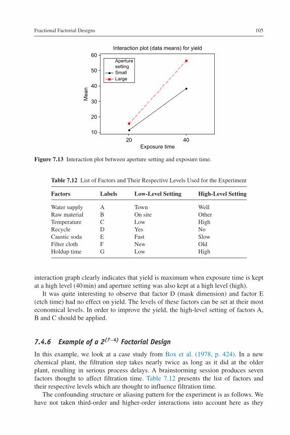
Fractional Factorial Designs 105
interaction graph clearly indicates that yield is maximum when exposure time is kept at a high level (40 min) and aperture setting was also kept at a high level (high).
It was quite interesting to observe that factor D (mask dimension) and factor E (etch time) had no effect on yield. The levels of these factors can be set at their most economical levels. In order to improve the yield, the high-level setting of factors A, B and C should be applied.
7.4.6 Example of a 2(7−4) Factorial Design
In this example, we look at a case study from Box et al. (1978, p. 424). In a new chemical plant, the filtration step takes nearly twice as long as it did at the older plant, resulting in serious process delays. A brainstorming session produces seven factors thought to affect filtration time. Table 7.12 presents the list of factors and their respective levels which are thought to influence filtration time.
The confounding structure or aliasing pattern for the experiment is as follows. We have not taken third-order and higher-order interactions into account here as they
Table 7.12 List of Factors and Their Respective Levels Used for the Experiment
Factors Labels Low-Level Setting High-Level Setting
Water supply A Town WellRaw material B On site OtherTemperature C Low HighRecycle D Yes NoCaustic soda E Fast SlowFilter cloth F New OldHoldup time G Low High
Exposure time
Mea
n
4020
60
50
40
30
20
10
AperturesettingSmallLarge
Interaction plot (data means) for yield
Figure 7.13 Interaction plot between aperture setting and exposure time.

Design of Experiments for Engineers and Scientists106
are usually negligible compared to the main and second-order interaction effects (Bisgaard, 1988).
A BD CE FG; B AD CF EG
C AE BF DG; D AB CG EF
E AC BG DF; F AG BBC DE
G AF BE CD
Each factor was studied at 2-levels. Due to time and cost constraints, it was decided to perform a 2(7−4) factorial design which is 1/16th fractional of a full facto-rial design. This clearly implies that we are studying 7 factors in 8 trials instead of 128 trials. Table 7.13 presents the experimental layout for the experiment.
Figure 7.14 shows a normal plot of all main effects (Daniel, 1976) which indi-cated that factors E and C appeared to have a significant effect on filtration time.
Effect
Per
cen
t
1050–5–10–15–20–25
99
95
90
80
7060504030
20
10
5
1
Caustic soda
Temperature
NPP of the effects(response is filtration time, alpha = 0.10)
Effect typeNot significantSignificant
Figure 7.14 NPP of effects.
Table 7.13 Experimental Layout for the Filtration Time Experiment
Trial No. A B C D E F G Filtration Time
1 Town On site Low No Slow Old Low 68.42 Well On site Low Yes Fast Old High 77.73 Town Other Low Yes Slow New High 66.44 Well Other Low No Fast New Low 81.05 Town On site High No Fast New High 78.66 Well On site High Yes Slow New Low 41.27 Town Other High Yes Fast Old Low 68.78 Well Other High No Slow Old High 38.7

Fractional Factorial Designs 107
However, factor E is confounded with two-order or second-order interactions such as AC, BG and DF. Similarly, factor C is confounded with AE, BF and DG. In such circumstances, we need to perform a fold-over design to separate out the main effects from interaction effects; this way we would know if it is the main effects or the interaction effects which influence the filtration time. The results of the fold-over design are given in Table 7.14. By using a fold-over design, we can de-alias the main effects. After the fold-over design was created and executed based on Table 7.14, the main effects were no longer confounded with second-order or two-factor interactions. However, two-factor interactions were still confounded with each other. Further analysis has showed that two effects appeared to be significant: the main effect due to factor E and the two-factor interaction AE. It was quite interesting to observe that temperature (factor C) was not a significant factor after all. One of the key findings of the experiment was that temperature had no significant effect on fil-tration time.
7.4.7 Another Example of a 2(7 − 4) Factorial Design
The determination of the moulding condition in an injection moulding process is very complicated. Typical injection moulding machines have many adjustable parameters which could potentially influence the quality of finished plastic parts. Quality can be determined in terms of dimensional conformity, appearance of the finished product or even mechanical characteristics. The traditional approach to determine the best moulding condition has been through trial and error which is time consuming and not cost effective. One of the most efficient methods of pro-cess optimisation and systematic investigation of the process is through the utilisa-tion of DOE. The plastic part for this example is the closure for infusion bottles. For more information about the case study, please refer to Azeredo et al. (2003), Improve moulded part quality, Quality Progress, July, pp. 72–76. The closure is moulded in high-density polyethylene and has complex geometry plus many functional prop-erties. For this experiment, the mould engineers were interested to understand the influence of moulding process parameters on the force needed to open the closure. Extremely high forces make it difficult to open the closure and low forces can result in damage during shipping or handling.
Table 7.14 Results of Fold-Over Design
Trial No. A B C D E F G Filtration Time
1 Well Other High Yes Fast New High 66.72 Town Other High No Slow New Low 65.03 Well On site High No Fast Old Low 86.44 Town On site High Yes Slow Old High 61.95 Well Other Low Yes Slow Old Low 47.86 Town Other Low No Fast Old High 59.07 Well On site Low No Slow New High 42.68 Town On site Low Yes Fast New Low 67.6
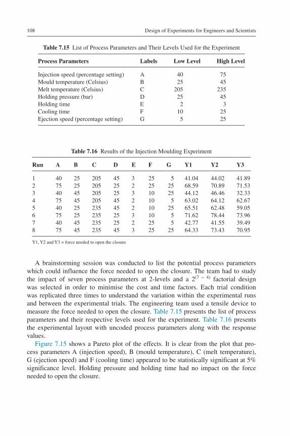
Design of Experiments for Engineers and Scientists108
A brainstorming session was conducted to list the potential process parameters which could influence the force needed to open the closure. The team had to study the impact of seven process parameters at 2-levels and a 2(7 − 4) factorial design was selected in order to minimise the cost and time factors. Each trial condition was replicated three times to understand the variation within the experimental runs and between the experimental trials. The engineering team used a tensile device to measure the force needed to open the closure. Table 7.15 presents the list of process parameters and their respective levels used for the experiment. Table 7.16 presents the experimental layout with uncoded process parameters along with the response values.
Figure 7.15 shows a Pareto plot of the effects. It is clear from the plot that pro-cess parameters A (injection speed), B (mould temperature), C (melt temperature), G (ejection speed) and F (cooling time) appeared to be statistically significant at 5% significance level. Holding pressure and holding time had no impact on the force needed to open the closure.
Table 7.15 List of Process Parameters and Their Levels Used for the Experiment
Process Parameters Labels Low Level High Level
Injection speed (percentage setting) A 40 75Mould temperature (Celsius) B 25 45Melt temperature (Celsius) C 205 235Holding pressure (bar) D 25 45Holding time E 2 3Cooling time F 10 25Ejection speed (percentage setting) G 5 25
Table 7.16 Results of the Injection Moulding Experiment
Run A B C D E F G Y1 Y2 Y3
1 40 25 205 45 3 25 5 41.04 44.02 41.892 75 25 205 25 2 25 25 68.59 70.89 71.533 40 45 205 25 3 10 25 44.12 46.46 32.334 75 45 205 45 2 10 5 63.02 64.12 62.675 40 25 235 45 2 10 25 65.51 62.48 59.056 75 25 235 25 3 10 5 71.62 78.44 73.967 40 45 235 25 2 25 5 42.77 41.55 39.498 75 45 235 45 3 25 25 64.33 73.43 70.95
Y1, Y2 and Y3 = force needed to open the closure
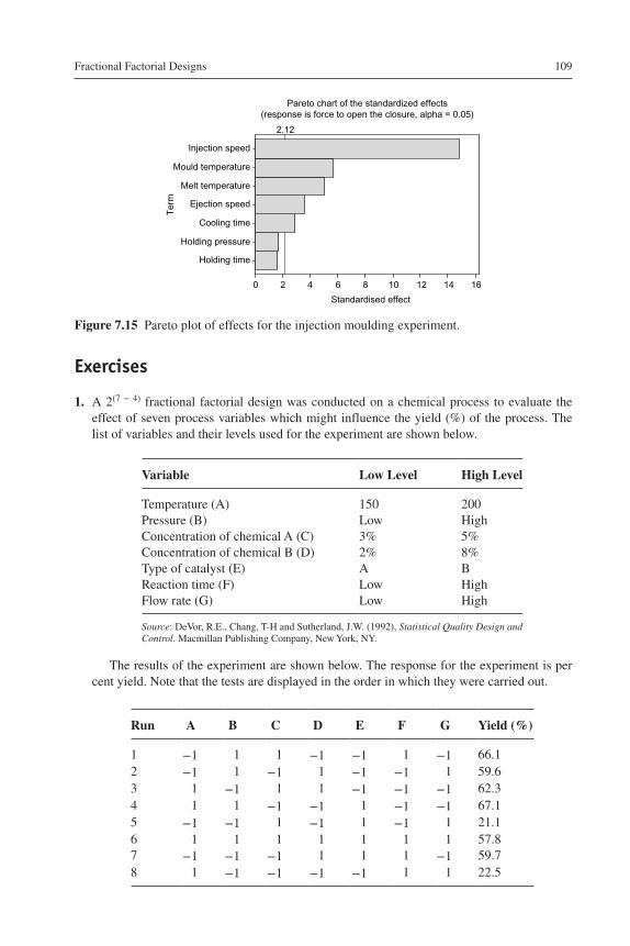
Fractional Factorial Designs 109
Exercises
1. A 2(7 − 4) fractional factorial design was conducted on a chemical process to evaluate the effect of seven process variables which might influence the yield (%) of the process. The list of variables and their levels used for the experiment are shown below.
Variable Low Level High Level
Temperature (A) 150 200Pressure (B) Low HighConcentration of chemical A (C) 3% 5%Concentration of chemical B (D) 2% 8%Type of catalyst (E) A BReaction time (F) Low HighFlow rate (G) Low High
Source: DeVor, R.E., Chang, T-H and Sutherland, J.W. (1992), Statistical Quality Design and Control. Macmillan Publishing Company, New York, NY.
The results of the experiment are shown below. The response for the experiment is per cent yield. Note that the tests are displayed in the order in which they were carried out.
Run A B C D E F G Yield (%)
1 −1 1 1 −1 −1 1 −1 66.12 −1 1 −1 1 −1 −1 1 59.63 1 −1 1 1 −1 −1 −1 62.34 1 1 −1 −1 1 −1 −1 67.15 −1 −1 1 −1 1 −1 1 21.16 1 1 1 1 1 1 1 57.87 −1 −1 −1 1 1 1 −1 59.78 1 −1 −1 −1 −1 1 1 22.5
Ter
m
Standardised effect
Holding time
Holding pressure
Cooling time
Ejection speed
Melt temperature
Mould temperature
Injection speed
1614121086420
2.12
Pareto chart of the standardized effects(response is force to open the closure, alpha = 0.05)
Figure 7.15 Pareto plot of effects for the injection moulding experiment.

Design of Experiments for Engineers and Scientists110
(a) What are the generators and defining relation for this experiment?(b) Illustrate the complete confounding structure for the design, assuming third-order and
higher-order interactions are negligible.(c) Which factor or interaction effects appear to have a significant impact on percentage
yield?(d) Construct a Pareto plot of effects and determine the optimal settings of the variables
which give maximum yield.(e) How do you validate the assumption of normality?
2. An experimenter decided to study the effect of four process parameters for an injection moulding process. The experimenter was interested in both main and two-factor interac-tions. The response of interest was the width of the injected part (accuracy is up to four decimal places), which is critical to customers. The results of the experiment are given in the following table. The experiment was repeated twice to create sufficient degrees of free-dom for the error term. The four process variables are D = mould temperature, A = injec-tion speed, E = hold pressure and B = cooling time.
Trial No. D A E B = DAE Width
1 −1 −1 −1 −1 9.3415 9.34162 −1 −1 1 1 9.3691 9.36923 −1 1 −1 −1 9.3467 9.34664 −1 1 1 −1 9.3680 9.36815 1 −1 −1 1 9.3679 9.36806 1 −1 1 −1 9.3493 9.34947 1 1 −1 1 9.3668 9.36698 1 1 1 1 9.3544 9.3545
Source: Schmidt, S.R. and Launsby, R.G. (1992), Understanding Industrial Designed Experiments. Air Academy Press, Colorado Springs, CO.
(a) What is the resolution of this design?(b) Display the complete confounding structure.(c) Which effects appear to have a significant effect on the width?(d) What are the best settings of the parameters to achieve a target width of 9.380?
3. An experimenter is interested in studying the effect of five welding process parameters. The results of the experiment are illustrated below. The response of interest to the experi-menter is heat input (measured in watts) for welding. The welding parameters considered for the experiment are A = open-circuit voltage, B = slope, C = electrode melt-off rate, D = electrode diameter and E = electrode extension.
The design matrix of the experiment with response is given in the following table.
Trial No. A B C D E Heat Input (W)
1 (12) −1 −1 −1 −1 1 33182 (1) 1 −1 −1 −1 −1 41413 (2) −1 1 −1 −1 −1 37904 (6) 1 1 −1 −1 1 40615 (15) −1 −1 1 −1 −1 34316 (8) 1 −1 1 −1 1 3425
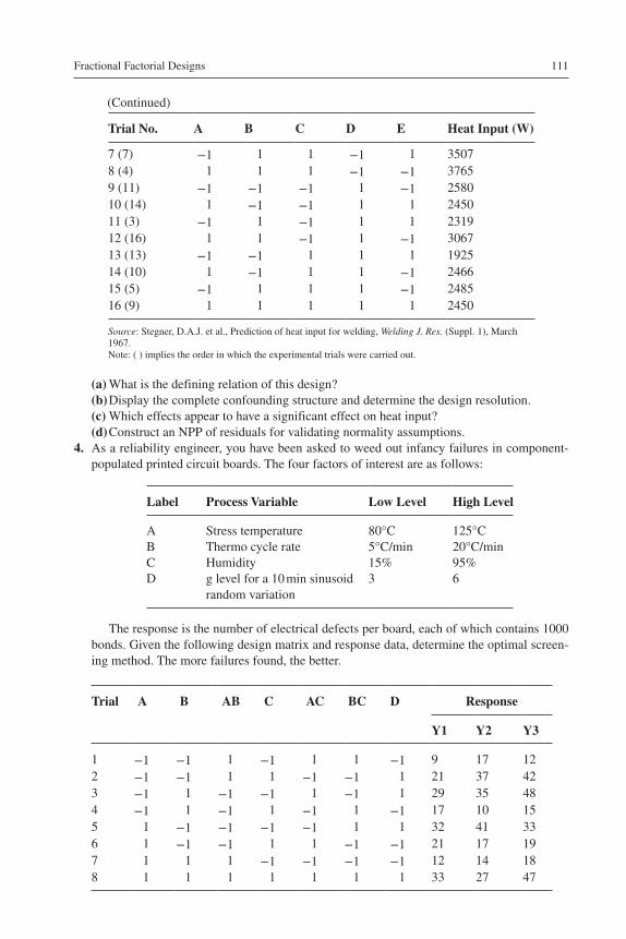
Fractional Factorial Designs 111
Trial No. A B C D E Heat Input (W)
7 (7) −1 1 1 −1 1 35078 (4) 1 1 1 −1 −1 37659 (11) −1 −1 −1 1 −1 258010 (14) 1 −1 −1 1 1 245011 (3) −1 1 −1 1 1 231912 (16) 1 1 −1 1 −1 306713 (13) −1 −1 1 1 1 192514 (10) 1 −1 1 1 −1 246615 (5) −1 1 1 1 −1 248516 (9) 1 1 1 1 1 2450
Source: Stegner, D.A.J. et al., Prediction of heat input for welding, Welding J. Res. (Suppl. 1), March 1967.Note: ( ) implies the order in which the experimental trials were carried out.
(a) What is the defining relation of this design?(b) Display the complete confounding structure and determine the design resolution.(c) Which effects appear to have a significant effect on heat input?(d) Construct an NPP of residuals for validating normality assumptions.
4. As a reliability engineer, you have been asked to weed out infancy failures in component-populated printed circuit boards. The four factors of interest are as follows:
Label Process Variable Low Level High Level
A Stress temperature 80°C 125°CB Thermo cycle rate 5°C/min 20°C/minC Humidity 15% 95%D g level for a 10 min sinusoid
random variation3 6
The response is the number of electrical defects per board, each of which contains 1000 bonds. Given the following design matrix and response data, determine the optimal screen-ing method. The more failures found, the better.
Trial A B AB C AC BC D Response
Y1 Y2 Y3
1 −1 −1 1 −1 1 1 −1 9 17 122 −1 −1 1 1 −1 −1 1 21 37 423 −1 1 −1 −1 1 −1 1 29 35 484 −1 1 −1 1 −1 1 −1 17 10 155 1 −1 −1 −1 −1 1 1 32 41 336 1 −1 −1 1 1 −1 −1 21 17 197 1 1 1 −1 −1 −1 −1 12 14 188 1 1 1 1 1 1 1 33 27 47
(Continued)

Design of Experiments for Engineers and Scientists112
References
Bisgaard, S., 1988. A Practical Aid for Experimenters. Starlight Press, Madison, WI.Box, G.E.P., Hunter, W.G., Hunter, J.S., 1978. Statistics for Experimenters. John Wiley &
Sons, New York, NY.Box, G.E.P., 1992. What can you find out from eight experimental runs? Qual. Eng. 4 (4),
619–627.Chow, E.T.S., Wei, L.S., De Vor, R.E., Steinberg, M.P., 1983. Application of a two-level frac-
tional factorial design in the development of a soybean whipped topping. J. Food Sci. 48 (1), 230–234.
Daniel, C., 1976. Applications of Statistics to Industrial Experimentation. John Wiley & Sons, New York, NY.
Drain, D., 1997. Handbook of Experimental Methods for Process Improvement. Chapman and Hall, London, UK.

Design of Experiments for Engineers and Scientists. DOI: Copyright © 2014 Jiju Antony. Published by Elsevier Ltd. All rights reserved.
http://dx.doi.org/10.1016/B978-0-08-099417-8.00008-0
Some Useful and Practical Tips for Making Your Industrial Experiments Successful
8
8.1 Introduction
Experimental Design (ED), or DOE, is a powerful approach to achieve increased understanding of your process, leading to significant improvements in product qual-ity, decreased manufacturing costs and potentially thousands of dollars of savings for organisations. So why don’t more manufacturers use ED? Why do some manufactur-ing companies try ED, and then abandon it, saying ‘It won’t work for us’? Inadequate training, demanding production schedules or time pressures, cost and resources required for the execution of an experiment or a series of experiments are often cited as the prin-cipal reasons. Moreover, fear of statistics is widespread, even among many educated scientists and managers in organisations. This chapter provides some useful and practi-cal tips for industrial engineers and managers with limited knowledge of ED or DOE for making industrial experiments successful in their own organisations. The purpose of this chapter is to stimulate the engineering community to start applying ED for tackling quality control problems in key processes they deal with everyday.
Industrial experiments are fundamental to and crucial for increasing the understanding of a process and of product behaviour. The success of any industrial experiment depends on a number of key factors such as statistical skills, engineering skills, planning skills, communication skills, teamwork skills and so on. Many scientists and engineers perform industrial experiments based on full and fractional factorial designs (Montgomery, 1991) or Orthogonal Array (OA) designs (Taguchi, 1986) for improving product quality and process efficiency. In other words, engineers and managers of today’s modern industrial world have placed an increased emphasis on achieving breakthrough improvements in product and process quality using DOE/ED. DOE/ED is essentially a strategy of industrial experimentation whereby one may vary a number of factors in a process/system simul-taneously to study their effect on the process/system output (Antony, 1996). DOE/ED is a direct replacement of traditional One-Factor-At-A-Time (OFAT) or the ‘Hit or Miss’ approach to experimentation (Antony, 1998). It is important to note that these tips were developed strictly on the basis of author’s experience and expertise in the field of study and also by reviewing many industrial case studies and literature in the subject matter.
8.1.1 Get a Clear Understanding of the Problem
One of the key reasons for an industrial experiment to be unsuccessful is due to lack of understanding of the problem itself. The nature of the experiment to be conducted

Design of Experiments for Engineers and Scientists114
is heavily dependent on the nature of the problem and the objective of the experiment. Therefore, it is absolutely essential to have a clear definition of both before one embarks on to any kind of experimentation. A well-defined objective leads the experimenter to the correct choice of ED. If you incorrectly state the objective(s) of an experiment, you may have to face the consequences – trying to study too many or too few factors for the experi-ment, not measuring the right quality characteristics or responses, or arriving at conclu-sions which are already known to the team conducting the experiment. In other words, unclear objectives can lead to lost time and money, as well as lack of appreciation and feelings of frustration for all involved in the study (Antony, 1997). Industrial experiments are generally a team effort; a typical team includes people from design and from the qual-ity and production department as well as an operator. It is quite important that everyone on the team have a clear understanding of the objective of the experiment and also of their role in experimentation. If there is more than one objective, it is then important to assign a relative weight to the objectives and establish ways in which each will be evaluated.
8.1.2 Project Selection
Selection of the right project will either assure you of success or guarantee an opportu-nity to try it again a second time. Many companies are continuously engaged in a num-ber of ED projects and it is important to identify the projects that can return the most savings. In situations where you have a number of experiments to be performed for a variety of problems, it is worthwhile to keep the following factors in mind.
Management Involvement and Commitment
Management must be involved in the project right from the beginning. You need their support and commitment when you need to take actions to improve a process or system. There is no point in pursuing a DOE/ED project if you do not have 100% backup from senior management team. Moreover, the purpose of the DOE/ED project must be clearly communicated to the senior management team and expectations regarding their involve-ment and commitment should be explicitly stated up front (Anderson and Kraber, 1999).
Return on Investment
Experimentation in general is not a priority for many senior managers in organisations. In fact, it is not an easy task for engineers to suggest DOE/ED to senior management as the solution to a particular problem. When you have a number of experiments to be carried out, consider the return on investment. Savings from reduced warranty costs, reduced customer complaints and increased customer satisfaction may produce a higher return in the long term. It is strongly advisable to present successful case studies of DOE from other businesses similar to yours.
Project Scope
If the system or process you deal with for experimentation purposes is too intricate in nature, it is best to break it down into sub-systems or sub-processes. For example, in
Some Useful and Practical Tips for Making Your Industrial Experiments Successful 115
the case of automobiles, rather than optimising the entire vehicle, it is better to start optimising the braking or suspension system. If it is feasible and practical, you may break the braking system into many sub-systems and seek to optimise the surface fin-ish of the rotor disk. Moreover, it is quite important to understand the boundaries of the project before it turns into a ‘boiling-the-ocean’ project.
Time Required to Complete the Project
An unfinished experiment is a waste of time and resources, and this can be quite det-rimental to all future initiatives. Therefore, it is important to start off with projects that bring quick wins to the organisation in a short time. This helps to boost the morale of the team and helps them to become more confident in undertaking more and more pro-jects across the organisation.
Value to Your Organisation
You should select a project that adds long-term value to the future of your organisation. Carry out DOE/ED projects (in the form of experiments) to achieve greater product performance that your customers may not be asking for now but may ask for soon. It is also highly desirable to select a project that is aligned with the strategic objectives of the business; this gives you a competitive advantage. For instance, select DOE/ED projects so that products can be introduced to market faster than those of your competi-tors. Understanding what makes the customer tick, anticipating his needs and behav-iours and then optimising products and service levels to meet all of these is the way ahead in business.
8.1.3 Conduct Exhaustive and Detailed Brainstorming Sessions
Many DOE/ED training courses and textbooks spend as much as 70–80% of their time in the analysis of experimental data gathered by the experimenter (i.e. statistical skills). The successful application of DOE/ED in today’s industrial environment requires a mixture of statistical, planning, engineering, communication and teamwork skills. Brainstorming must be treated as an integral part of the planning and design of effec-tive experiments (Bhote, 1988). There is no standard procedure on how to perform a typical brainstorming session that is applicable to all industrial situations. The nature and content of each brainstorming session will rely heavily on the nature of the prob-lem under investigation. In the context of DOE/ED, brainstorming is performed with the following purposes and questions in mind:
● Identification of the factors, the number of levels and other relevant information about the experiment.
● Development of team spirit and positive attitude in order to assure greater participation of the team members.
● How well does the experiment simulate the customers or users conditions?● Who will do what and how? For example, who will be responsible for data analysis?● How quickly does the experimenter need to provide the results to the management?● Is experimentation the only way to tackle the problem at hand?

Design of Experiments for Engineers and Scientists116
8.1.4 Teamwork and Selection of a Team for Experimentation
For ED projects, it is good practice to have a project owner who is responsible for team formation. In selecting team members, the following criteria may be considered:
● Project beneficiaries – These are people who must accept your recommendation for improvement further to key findings from the experiment. They may not be directly involved in the project, but it is important to bring them in the loop somehow.
● Parts/materials supplier – If the parts/materials supplier is a factor in the experiment, it is best to consult with them and include them on the experimentation team.
● Direct involvement – When planning and conducting an experiment, it is important to include people who can provide input into the identification of factors for the experiment. For a typical industrial designed experiment, personnel involved in design, validation, quality and production, as well as operators, are likely candidates (Anderson, 2000).
8.1.5 Select the Continuous Measurable Quality Characteristics or Responses for the Experiment
A quality characteristic or response is the performance characteristic of a product that is most critical to customers and often reflects the product quality. Selecting the right quality characteristic (or response) is critical to the success of any industrial designed experiment (Antony, 1998). Many DOE programs fail because their responses can-not be measured quantitatively. A classic example can be found with the traditional approach to evaluating quality, where an inspector uses a subjective judgement based on his experience to determine whether a product or unit passes or fails the test. Pass/fail data can be used in DOE, but it is very crude and inefficient. For example, if your process typically produces a 0.5% defect rate, you would expect to find 5 out of 1000 parts defective. If you perform a 16-trial experiment, you would then require a mini-mum of 16,000 parts (16 × 1000). This poses the question, ‘Can we afford the cost associated with the parts?’
The following guidelines may be useful to engineers in selecting the quality char-acteristics or responses for industrial experiments:
● Use quality characteristics (or responses) that can be measured accurately and with stability.
● Use quality characteristics that can be measured quantitatively.● Use quality characteristics which are directly related to the energy transfer associated with
the fundamental mechanism of the product or the process.● Use quality characteristics which are complete, i.e. they should cover the input–output
relationship for the product or the process.● For complex systems or processes, select quality characteristics at the sub-system level and
perform experiments at this level before trying to optimise the overall system.
Consider a coating process which results in various problems such as poor appearance, low yield, orange peel and voids. Too often, experimenters measure these characteristics as data and try to optimise the response. This is not sound engi-neering, because these are the symptoms of poor function. It is not the function of the coating process to produce an orange peel. Problems such as orange peel are due

Some Useful and Practical Tips for Making Your Industrial Experiments Successful 117
to excessive variability of the coating process caused by noise factors such as vari-ability in viscosity, ambient temperature, etc. We should measure data that relate to the function itself, not the symptom of variability. One fairly good characteristic to measure for the coating process is the coating thickness. The aim of the coating pro-cess is to form the coating layer; effects such as orange peel result from excessive variability of coating thickness from its target. A sound engineering approach is to measure the coating thickness and determine the best settings of the coating process that will minimise the coating thickness variability around its target value. Table 8.1 provides a framework covering a variety of manufacturing process problems and the suitable response of interest to experimenters for each associated process.
In essence, the selection of attribute quality characteristics (e.g. good/bad, defective/non-defective, etc.) for industrial experiments is not a good practice. This does not mean that experimenters should measure only continuous measurable qual-ity characteristics. The author nevertheless recommends choosing continuous char-acteristics over attributes. One of the limitations with the attribute characteristic is its poor additivity. It means that many main effects will be confounded with two-factor interactions or that two-factor interactions will be confounded with other two-fac-tor interactions. Attribute characteristics also require a large number of samples and therefore experiments involving such characteristics are costly and time consuming.
8.1.6 Choice of an Appropriate ED
The choice of ED is very important for the success of any industrial experiment as it depends on various factors which include the nature of the problem at hand, the num-ber of factors to be studied, resources available for the experiment, time needed to complete the experiment and the resolution of the design. We can use either Classical
Table 8.1 Examples of Quality Characteristics for Various Manufacturing Processes
Type of Process Objective of the Experiment Appropriate Response
Extrusion To reduce the post extrusion shrinkage of a speedometer cable casing
Shrinkage
Coil spring manufacturing To reduce variability in the tension of coil springs
Spring tension
TV picture tube manufacturing
To reduce performance variation of TV electron guns
Cut-off voltage
Surface mounting To improve field reliability Shear strengthGold plating To reduce variation in gold plating
thicknessPlating thickness
Die-casting process To increase the hardness of a die-cast engine component
Rockwell hardness
MIG welding To reduce the high scrap rate due to poor welded joints
Weld strength
Wire bonding To reduce the defect rate from broken wires
Wire pull strength

Design of Experiments for Engineers and Scientists118
ED (full and fractional factorial designs), advocated by Sir Ronald Fisher, or OA designs, recommended by Dr Taguchi (Antony, 1999). In Classical ED, the focus is on the study of product and process behaviour, followed by the development of a math-ematical model which explicitly illustrates the relationship between a dependent vari-able and a set of independent variables. Experiments based on OA designs, promoted by Taguchi, are focused on product and process robustness. Here robustness refers to reducing the process/product performance to noise sensitivity. Taguchi recommends the use of the SNR to estimate the performance sensitivity of a product to noise. The choice of any of these designs will be dependent upon the following factors:
● degree of optimisation required for the chosen quality characteristic● number of factors and interactions (if any) to be studied● complexity of using each design● statistical validity and effectiveness of each design● degree of product/process functional performance robustness to be attained from the
experiment● ease of understanding and implementation● nature of the problem (or objective of the experiment)● cost and time constraints.
The interesting thing is that many companies the author has visited rely on just one approach of DOE. So whenever the author approaches the Engineering Director, Operations Director or Manufacturing Director in local companies, the author often gets the response, “Our employees have been trained on Taguchi or Classical DOE.” As mentioned above, you cannot use the same approach for all problems in the busi-ness. The solution to a problem depends upon the nature of the problem. For instance, if a company wants to achieve robust performance due to inconsistency issues from the presence of noise factors in the process, it is best to look into an RPD, as expounded by Dr Taguchi. On the other hand, if your objective is to predict performance based on a regression model with quadratic effects (non-linear effects), it is probably best to look into Classical DOE followed by the use of Response Surface Methodology (RSM) (Box et al., 1978).
8.1.7 Iterative Experimentation
Experiments should be conducted in an iterative manner so that information gained from one experiment can be applied to the next. It is best to run a number of smaller and sequential experiments rather than running a large experiment with several factors and using up the majority of resources assigned to the experimentation process. If none of the factors or process variables is significant, the experiment would then be a waste of time and money. The first step in any experimentation process is to ‘separate out the vital few from the trivial many’. Screening experiments are generally performed to reduce the number of factors or key process variables to a manageable number in a limited number of experimental trials (Hansen, 1996).
It is advisable not to invest more than 25% of the experimental budget in the first phase of any experimentation, such as screening (Montgomery, 1991). Once the key factors have been identified, the interactions among them can be studied using full or

Some Useful and Practical Tips for Making Your Industrial Experiments Successful 119
fractional factorial experiments. Once you identify the key variables and interactions for a process, you may then want to perform an RSM, which allows you to model the process behaviour over its entire operating region. Using RSM, one may be able to develop a second-order mathematical model that depicts the relationship between the key process variables and the process response. This model can then be used to predict the values of the responses at different variable settings.
8.1.8 Randomise the Experimental Trial Order
In the context of ED, randomisation is a process of performing experimental trials in a random order in which they are logically listed. This is a very important concept in any ED because an experimenter cannot always be certain that all important factors affecting a response have been included and considered in the experiment. The purpose of randomisation is to reduce the systematic bias that is induced into the experiment (Kraber, 1998). The bias may be due to the effect of uncontrolled factors or noise, such as machine ageing, changes in raw material, tool wear, change of relative humidity, power surges, change of ambient temperature and so on. These changes, which often are time related, can significantly influence the response. For example, assume that an experiment is performed so that all the low levels of factor A are run first, followed by the high levels of factor A. During the course of the experiment, the humidity in the workplace changes by 50%, creating a significant effect on the response. The analy-sis may reveal that factor A is statistically significant. In reality factor A is not sig-nificant; it is the change in humidity level that caused the factor effect to be significant. Randomisation would have prevented this confusion.
Whilst conducting an experiment, do not underestimate the background noise inher-ent in the experiment. Characterisation of the noise variables allows an engineer to understand their effect and minimise their influence on the process performance. A fac-tor may turn out to be significant due to the influence of the lurking variables (or noise variables), which often are uncontrollable. Randomisation will minimise the effect of a factor which has been confounded with the effect of noise. The author therefore recom-mends that the experimenters randomise (if possible) the trials.
8.1.9 Replicate to Dampen the Effect of Noise or Uncontrolled Variation
Replication improves the chance of detecting a statistically significant effect (i.e. signal) in the midst of natural process variation. In some processes, the amount of natural process variation is very large. This can mitigate your chances of detecting a significant factor or interaction effect. One of the common queries before conducting experiments in organisations is ‘How many experimental runs are required to identify significant effect(s), given the current process variation?’ SNRs help to determine the minimum number of experimental runs needed to achieve a given power for your ED (Taguchi and Yokoyama, 1993). The signal is the change in response that you want to detect. You need to determine the smallest change you want to detect. Once the signal is detected, you may then estimate the noise. Here noise is the random variation that occurs in the response during standard operating conditions. The noise (i.e. measure
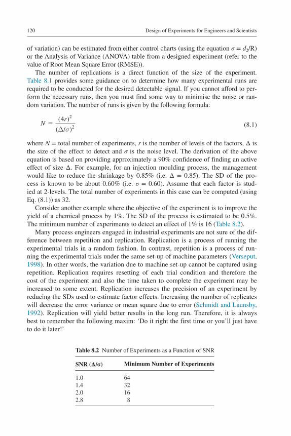
Design of Experiments for Engineers and Scientists120
of variation) can be estimated from either control charts (using the equation σ = d2/R) or the Analysis of Variance (ANOVA) table from a designed experiment (refer to the value of Root Mean Square Error (RMSE)).
The number of replications is a direct function of the size of the experiment. Table 8.1 provides some guidance on to determine how many experimental runs are required to be conducted for the desired detectable signal. If you cannot afford to per-form the necessary runs, then you must find some way to minimise the noise or ran-dom variation. The number of runs is given by the following formula:
Nr
�( )
( )
4 2
2∆/σ
where N = total number of experiments, r is the number of levels of the factors, Δ is the size of the effect to detect and σ is the noise level. The derivation of the above equation is based on providing approximately a 90% confidence of finding an active effect of size Δ. For example, for an injection moulding process, the management would like to reduce the shrinkage by 0.85% (i.e. Δ = 0.85). The SD of the pro-cess is known to be about 0.60% (i.e. σ = 0.60). Assume that each factor is stud-ied at 2-levels. The total number of experiments in this case can be computed (using Eq. (8.1)) as 32.
Consider another example where the objective of the experiment is to improve the yield of a chemical process by 1%. The SD of the process is estimated to be 0.5%. The minimum number of experiments to detect an effect of 1% is 16 (Table 8.2).
Many process engineers engaged in industrial experiments are not sure of the dif-ference between repetition and replication. Replication is a process of running the experimental trials in a random fashion. In contrast, repetition is a process of run-ning the experimental trials under the same set-up of machine parameters (Verseput, 1998). In other words, the variation due to machine set-up cannot be captured using repetition. Replication requires resetting of each trial condition and therefore the cost of the experiment and also the time taken to complete the experiment may be increased to some extent. Replication increases the precision of an experiment by reducing the SDs used to estimate factor effects. Increasing the number of replicates will decrease the error variance or mean square due to error (Schmidt and Launsby, 1992). Replication will yield better results in the long run. Therefore, it is always best to remember the following maxim: ‘Do it right the first time or you’ll just have to do it later!’
(8.1)
Table 8.2 Number of Experiments as a Function of SNR
SNR (Δ/σ) Minimum Number of Experiments
1.0 641.4 322.0 162.8 8

Some Useful and Practical Tips for Making Your Industrial Experiments Successful 121
8.1.10 Improve the Efficiency of Experimentation Using a Blocking Strategy
Blocking can be used to minimise the chances of experimental results being influenced by variations from shift to shift, day to day or machine to machine. By dividing your experimental runs into homogeneous blocks and then arithmetically removing the dif-ference, you increase the sensitivity of your experiment. Do not block on anything that you want to study. For example, if you want to measure the difference in the quality of materials provided by three suppliers, then you have to include ‘supplier’ as a factor in your experiment. When blocking occurs, one or more of the interactions is likely to be confounded with the block effects; however, a good choice of blocking should ensure that it is a higher-order interaction (one that would be challenging to interpret or is not be expected to be important) that is confounded.
The blocks can be batches of different shifts, different machines, raw materials and so on. Shainin’s Multi-variate charts can be a useful tool for identifying those variables that cause unwanted sources of variability. For example, a metallurgist wishes to improve the strength of a certain steel component. Four factors at 2-levels each were considered for the experiment. An eight-trial experiment was chosen, but it was possible to run only four experimental trials per day. Hence each day was treated was treated as a separate block, with the purpose of reducing day-to-day vari-ation. It is important that the experimental trials within the block be as homogeneous as possible.
In the context of ED, one usually has to obtain blocking generator(s) prior to apply-ing a blocking strategy. In order to obtain the blocking generators, it is advised to decide on the number of blocks needed for the experiment as well as the block size. It is important to ensure that the block generators are not confounded with the main effects or with two-factor interaction effects. Box et al. (1978) provide a useful table which illustrates the number of blocks, block size, recommended block generators, the number of experimental trials and the resolutions of the blocked design.
8.1.11 Understanding the Confounding Pattern of Factor Effects
The confounding pattern is often overlooked by many experimenters who use Taguchi OA designs, Plackett–Burmann designs or highly fractionated factorial designs. If we study three factors at 2-levels using four runs, the main effects will be confounded with two-factor interactions. In other words, the estimates of main effects cannot be sep-arated out from the interactions. It is always dangerous to run such a low-resolution fractional factorial design. In the above case, we generally assign factor A to column 1, factor B to column 2 and factor C to column 3. In fact, column 3 can also be obtained due to the interaction between factors A and B. In other words, main effect C is con-founded with interaction AB. If column 3 is significant from the statistical analysis, then we don’t know whether the effect is the result of C, AB or both.
Confounding can be avoided by carefully choosing high-resolution fractional designs, but the cost factor will go up due to the large size of the experiment. The challenge here is to find the balance between the size of the experiment and the

Design of Experiments for Engineers and Scientists122
information gained from the experiment. An understanding of confounding struc-tures (also called alias structures) can be a tremendous asset to the experimenter.
8.1.12 Perform Confirmatory Runs/Experiments
There is a tendency to eagerly grab the results, rush out to production and say, ‘We have the answer! This will solve the problem!’ Before doing that, it is important to take the time to verify the outcome of your experiment using confirmatory runs. A con-firmatory run or experiment is necessary in order to verify the results of the experiment from the statistical analysis. If conclusive results have been obtained, it is then recom-mended to take improvement actions on the process under investigation. In contrast, if the results do not turn out as expected, further investigation would then be required (Taguchi, 1986). Some of the possible causes for not achieving the objective of the experiment include the following:
● wrong choice of ED for the experiment● incorrect choice of quality characteristic (or response) for the experiment● important factors that influence the response of interest are not as yet identified● presence of non-linear or curvature effect of factors on the response of interest● inadequate control of noise factors, causing unpleasant variation in the process under
investigation● measurement system error is very high● rushing into data analysis without understanding the details of assumptions behind the data
analysis● problem scope was not clearly understood by the team● lack of expertise on the part of the user in the statistical analysis.
Exercises
1. Explain why unclear experimental objectives can lead to lost time and money.2. What factors should be considered for the selection of an ED project?3. Why is brainstorming important in the context of ED?4. What are the advantages of choosing measurable quality characteristics over attribute
characteristics?5. Why must experiments be conducted in an iterative manner?6. Why is blocking important in industrial designed experiments?7. Why do we need to perform confirmatory runs/experiments?8. How do you differentiate between replication and repetition?9. What are the pros and cons of randomisation as a principle of ED?
References
Anderson, M.J., Kraber, S.L., 1999. Eight keys to successful DOE. Qual. Digest July (down-loaded from www.statease.com).
Anderson, M.J., 2000. Success with DOE. Quality 59 (4), 38–44.

Some Useful and Practical Tips for Making Your Industrial Experiments Successful 123
Antony, J., 1996. Likes and dislikes of Taguchi methods. J. Productivity 37 (3), 477–481.Antony, J., 1997. Experiments in quality. J. Manuf. Eng. IEE 76 (6), 272–275.Antony, J., 1998. Some key things industrial engineers should know about experimental
design. Log. Inf. Manag. 11 (6), 386–392.Antony, J., 1999. Ten useful and practical tips for making your experiments successful. TQM
Mag. 11 (4), 252–256.Bhote, K.R., 1988. DOE – the high road to quality. Manag. Rev., 27–33.Box, G., Hunter, W., Hunter, J.S., 1978. Statistics for Experimenters. John Wiley & Sons,
New York, NY.Hansen, R.C., 1996. Success with Designed Experiments for Industry. ASQ’s 50th Annual
Quality Congress Transactions, 13–15 May 1996, Chicago, USA, pp. 718–728.Kraber, S.L., 1998. Keys to Successful Designed Experiments. ASQ’s 52nd Annual Quality
Congress Transactions, May 4–6, Pennsylvania, pp. 119–123.Montgomery, D.C., 1991. Design and Analysis of Experiments. John Wiley & Sons,
New York, NY.Schmidt, S.R., Launsby, R.G., 1992. Understanding Industrial Designed Experiments. Air
Academy Press, Colorado Springs, CO.Taguchi, G., 1986. Introduction to Quality Engineering. Asian Productivity Organization,
Tokyo, Japan.Taguchi, G., Yokoyama, K., 1993. Taguchi Methods Design of Experiments. Quality
Engineering Series, vol 4. American Supplier Institute (ASI) Press, Tokyo, Japan.Verseput, R., 1998. DOE requires careful planning. R & D Mag., 71–72.

Design of Experiments for Engineers and Scientists. DOI: Copyright © 2014 Jiju Antony. Published by Elsevier Ltd. All rights reserved.2014
http://dx.doi.org/10.1016/B978-0-08-099417-8.00009-2
Case Studies9
9.1 Introduction
This chapter presents a collection of real industrial case studies. The case studies illus-trated in this chapter are well-planned experiments and not simply a few experimental trials to explore the effects of varying one or more factors at a time. The case studies will provide a good foundation for students, researchers and practitioners on how to go about carrying out an experiment in real industrial settings. The case studies will cover the nature of the problem or objective of the experiment, list of factors, their levels, response of interest, choice of a particular design (i.e. number of trials used), analysis using Minitab software, interpretation of results and benefits gained from the experiment. These case studies will increase the awareness of the application of ED techniques in industries and its potential in tackling process optimisation and variability problems.
9.2 Case Studies
9.2.1 Optimisation of a Radiographic Quality Welding of Cast Iron
Objective of the Experiment
The objective of the experiment was to identify the significant welding parameters and to determine the optimal parameter settings which gave minimum crack length.
Selection of the Response Function
The response of interest for the experiment was crack length measured in centimetres.
List of Factors and Interactions of Interest for the Experiment
Five main effects and 2 two-order interactions were identified from a thorough brain-storming session. The list of main and interaction effects is shown below.
Main effects: Current (A), Bead length (B), Electrode make (C), V-groove angle (D) and Welding method (E)
Interaction effects: A × B and B × C
Levels of Parameters and Their Ranges
Each parameter was studied at 2-levels. The ranges of welding parameters are given in Table 9.1.

Design of Experiments for Engineers and Scientists126
Choice of Design and Number of Experimental Trials
As the number of factors is more than four, it was decided to select a fractional factorial design rather than a full factorial design. The number of degrees of freedom for studying both main effects and interactions is equal to seven. The closest number of experimental trials that can be employed for this study is eight. This means it is a 2(5−2) fractional fac-torial design in which main effects are confounded with two-factor interactions. In other words, the design resolution of this design is III.
Design Generators and the Confounding Structure of the Design
Design generators: D AC and E ABC� �
De�ning relationship: I ACD I ABCE and I BDE� � �,
A CD BCE
B ACE DE
C AD ABE
Confounding pattern: D AC BE
E ABC BD
� �
� �
� �
� �
� �
AAB CE ADE BCD
AC BE, BC AE ABD CDE
� � �
� � � �
Uncoded Design Matrix with Response Values
The uncoded design matrix showing all the real factor settings, along with the respective response values, is given in Table 9.2. Each trial condition was replicated twice to create adequate degrees of freedom for the error term. Randomisation strat-egy was employed to minimise the effect of lurking variables and undesirable exter-nal influences induced into the experiment. As we can see from Table 9.2, welding parameter C (electrode make) was assigned to column 1 as it was not practical to change the levels of this factor frequently.
Table 9.1 List of Factors and Their Ranges for the Experiment
Welding Parameters Labels Low Level High Level
Current A 110 135Bead length B 20 30Electrode make C X YV-groove angle D 45 60Welding method E 1 2

Case Studies 127
Analysis and Interpretation of Results
The first step was to check the data for normality assumptions. This was achieved by constructing NPP of residuals (Figure 9.1). The plot suggests that the data fol-low a normal distribution. The analysis part involves the determination of significant main and interaction effects, followed by the selection of optimal welding parameter settings which yield minimum crack length. In order to identify the most important main and interaction effects, it was decided to use a Pareto plot of effects (Figure 9.2). Figure 9.2 indicates that main effects A and E and interaction effect BC were con-sidered to be real (or active). In order to analyse interaction between B and C, it was decided to use an interaction plot, shown in Figure 9.3.
Figure 9.3 indicates that there is a strong interaction between B and C. Moreover, it can be observed from Figure 9.3 that crack length is minimum when B is kept at a high-level setting and C at a low-level setting. In order to determine the opti-mal welding parameter settings that yield minimum crack length, a main effects plot
–1 0 1
–2
–1
0
1
2
Nor
mal
sco
re
Residual
Figure 9.1 NPP of residuals.
Table 9.2 Uncoded Design Matrix with Response Values
Standard Order C B A D = AC E = ABC Crack Length (cm)
1 (5) X 20 110 60 1 9, 122 (3) Y 20 110 45 2 7, 83 (8) X 30 110 60 2 7, 54 (2) Y 30 110 45 1 13.5, 12.05 (6) X 20 135 45 2 10, 96 (1) Y 20 135 60 1 6.5, 87 (7) X 20 135 45 1 7, 68 (4) Y 20 135 60 2 7.5, 8
Note: ( ) represents the order in which the experimental runs were carried out.

Design of Experiments for Engineers and Scientists128
is constructed (Figure 9.4). The optimal settings for minimising crack length are as follows:
A: +1 (high level)B: +1 (high level)C: −1 (low level)D: +1 (high level)E: +1 (high level)
Confirmatory Trials
Three confirmatory trials based on the optimal settings were performed and crack lengths of 0.31, 0.46 and 0.32 mm were observed. The results of the study have
–11
11–1
10.2
9.2
8.2
7.2
6.2
B
C
Mea
n cr
ack
leng
th
Figure 9.3 Interaction plot of B versus C.
0 1 2 3 4 5
B
C
AB
D
A
E
BC
Figure 9.2 Pareto plot of effects from the experiment.

Case Studies 129
demonstrated a significant improvement to the process and a significant reduction in scrap and rework was achieved.
9.2.2 Reducing Process Variability Using ED Technique
Objective of the Experiment
The objective of the experiment was to identify the most important process param-eters that affect variability in response.
Selection of the Response
The response of interest for the experiment was expulsion force measured in kilo-grams (kg). Here expulsion force is the force required to expel the device or compo-nent from a certain tube.
List of Process Parameters and Their Levels
Seven process parameters were identified from a brainstorming session with people from production, maintenance, quality, design and the shop floor. As part of the ini-tial investigation of the study, it was decided to study the main effects on variability in expulsion force. The parameters used for the experiment and their levels are illus-trated in Table 9.3.
Choice of Design and Number of Experimental Trials Required for the Experiment
For this study, seven factors were thought to have some impact on variability in expulsion force. An FFE would require a total of 128 experimental trials. Owing to limited budget and the top management needing a speedy response to this
C B A D E
7.7
8.1
8.5
8.9
9.3
Cra
ck le
ngth
–1 1 –1 1 –1 1 –1 1 1–1
Figure 9.4 Main effects plot for crack length.

Design of Experiments for Engineers and Scientists130
investigation, it was decided to use a highly fractionated factorial design. Here the objective was to identify the key process parameters so that further smaller experi-ments could be carried out to study the interactions among the key parameters. The number of degrees of freedom associated with seven factors at 2-levels is equal to 7. Hence the number of degrees of freedom required for the experiment must be greater than 7. The closest number of experimental trials that can be employed for this study is 8, that is, a 2(7−4) fractional factorial design was selected.
Design Generators and Resolution
C = −ABE = −ADF = −BDG = ABC
As the main effects are confounded with two-factor interactions, the resolution of this design is III.
Coded and Uncoded Design Matrix with Response Values
The uncoded and coded design matrices with response values are given in Tables 9.4 and 9.5. Each trial condition was repeated five times to analyse variability.
Table 9.3 List of Process Parameters and Their Levels
Process Parameters Labels Low Level High Level
Position of the cam A Forward (F) Backward (B)Drum temperature B 84 104Time C 68 72Type of material D 1 2Clearance E 0.006 0.012Machine alignment F 134 130Header temperature G 190 210
Table 9.4 Uncoded Design Matrix with Response Values
Run A B C D E F G Expulsion Force (kg)
1 F 84 68 1 0.006 134 190 0.990, 1.037, 0.965, 0.860, 1.0862 B 84 72 1 0.012 134 210 0.875, 0.748, 0.959, 0.600, 0.8073 F 104 72 1 0.006 130 210 0.924, 0.881, 0.733, 0.767, 0.8734 B 104 68 1 0.012 130 190 0.760, 0.620, 0.669, 0.632, 0.6055 F 84 68 2 0.012 130 210 0.741, 0.455, 0.549, 0.468, 0.6466 B 84 72 2 0.006 130 190 0.787, 1.061, 0.607, 1.168, 0.8787 F 104 72 2 0.012 134 190 0.508, 0.446, 0.351, 0.419, 0.4218 B 104 68 2 0.006 134 210 0.691, 0.771, 0.940, 0.743, 0.675

Case Studies 131
Analysis and Interpretation of Results
As the objective of the experiment is to reduce variability in expulsion force, the first step is to identify which of the seven factors have an impact on variability. In order to analyse variability, both SD and ln(SD) (natural logarithms of SD) were computed at each ED point. The results are given in Table 9.6.
An NPP of residuals was constructed for the validity of normality assumptions (Figure 9.5). Figure 9.5 shows that the data come from a normal population. Having checked the data for normality, the next step was to identify the factors which influ-ence variability in expulsion force. Both a main effects plot and a Pareto plot are used to identify the key process parameters or factors which have an impact on varia-bility. The graphs (Figures 9.6 and 9.7) indicate that factor B has a significant impact on variation. In order to obtain adequate degrees of freedom for the error variance term, a pooling strategy was utilised. The rule of thumb is to pool the effects with low magnitude till the error degrees of freedom is nearly half the total degrees of freedom. It was interesting to note that variability is minimum when factor B is kept at high level (Figure 9.7).
Table 9.5 Coded Design Matrix with Response Values
Run A B C D E F G Expulsion Force (kg)
1 −1 −1 −1 −1 −1 −1 −1 0.990, 1.037, 0.965, 0.860, 1.0862 1 −1 1 −1 1 −1 1 0.875, 0.748, 0.959, 0.600, 0.8073 −1 1 1 −1 −1 1 1 0.924, 0.881, 0.733, 0.767, 0.8734 1 1 −1 −1 1 1 −1 0.760, 0.620, 0.669, 0.632, 0.6055 −1 −1 −1 1 1 1 1 0.741, 0.455, 0.549, 0.468, 0.6466 1 −1 1 1 −1 1 −1 0.787, 1.061, 0.607, 1.168, 0.8787 −1 1 1 1 1 −1 −1 0.508, 0.446, 0.351, 0.419, 0.4218 1 1 −1 1 −1 −1 1 0.691, 0.771, 0.940, 0.743, 0.675
Table 9.6 SD and ln(SD) Values
Run A B C D E F G S ln(SD)
1 −1 −1 −1 −1 −1 −1 −1 0.085 −2.4652 1 −1 1 −1 1 −1 1 0.136 −1.9953 −1 1 1 −1 −1 1 1 0.081 −2.5134 1 1 −1 −1 1 1 −1 0.0621 −2.7795 −1 −1 −1 1 1 1 1 0.122 −2.1046 1 −1 1 1 −1 1 −1 0.222 −1.5057 −1 1 1 1 1 −1 −1 0.057 −2.8658 1 1 −1 1 −1 −1 1 0.106 −2.244
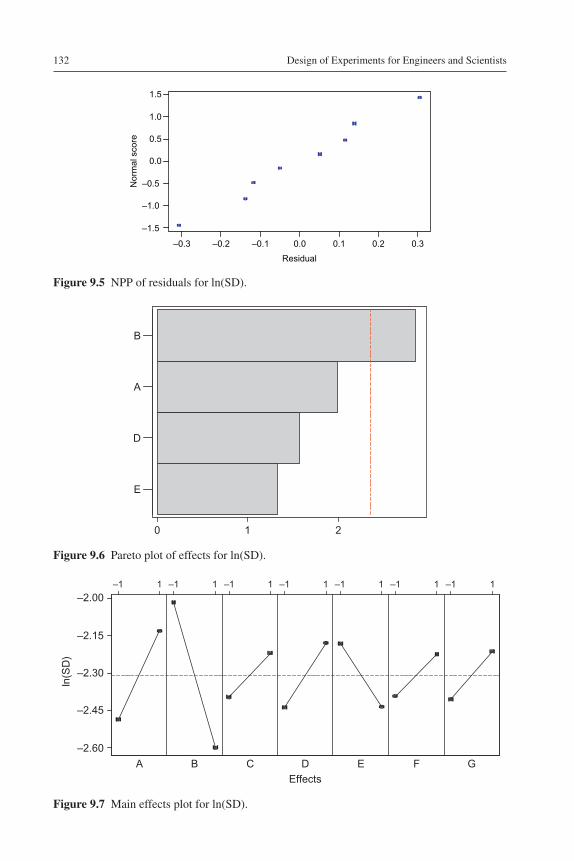
Design of Experiments for Engineers and Scientists132
210
B
A
D
E
Figure 9.6 Pareto plot of effects for ln(SD).
–0.3 –0.2 –0.1 0.0 0.1 0.2 0.3
–1.5
–1.0
–0.5
0.0
0.5
1.0
1.5
Nor
mal
sco
re
Residual
Figure 9.5 NPP of residuals for ln(SD).
A B C D E F G
–2.60
–2.45
–2.30
–2.15
–2.00
ln(S
D)
Effects
–1 1 –1 1 –1 1 –1 1 –1 1 –1 1 –1 1
Figure 9.7 Main effects plot for ln(SD).

Case Studies 133
Determination of Optimal Settings to Minimise Variability
In order to determine the optimal settings to minimise variability, the first step was to rank the factors (in descending order of importance) that influence variability in expulsion force.
Factor B – Rank 1Factor A – Rank 2Factor D – Rank 3Factor E – Rank 4Factor G – Rank 5Factor C – Rank 6Factor F – Rank 7
The optimal condition based on the main effects plot was obtained as follows:
B A D E G C F( ) ( ) ( ) ( ) ( ) ( ) ( )1 1 1 1 1 1 1� � � � �
Confirmation Trials
Fifteen samples were produced under the optimal conditions and compared against the samples produced under standard production conditions. The sample SD at the optimal settings was reduced to 0.042 kg as opposed to 0.125 kg under normal production con-ditions. The reduction in SD was therefore estimated to be approximately 66%.
Significance of the Work
Due to the significant reduction in process variability, the actual capability of the process has increased from 0.86 to over 1.78. This clearly demonstrates a dramatic improvement in the process performance and thereby more reliable and consistent products can be produced by determining the optimal condition of the process under study. The benefits from this study include increased customer satisfaction, reduced warranty costs, reduced customer complaints, reduced scrap and rework, improved market share, improved process control and so forth. The engineering team, includ-ing production personnel, quality engineers and managers of the company, are now well aware of the benefits that can be gained from the application of ED methods. Moreover, the awareness that has been established within the organisation has built confidence among the engineers, managers and front-line workers in other areas fac-ing similar difficulties.
9.2.3 Slashing Scrap Rate Using Fractional Factorial Experiments
Nature of the Problem
This case study describes the application of a highly fractionated factorial design to a manufacturing process that makes electromagnetic clutch coils. The coils were made of about 0.75 mm diameter copper wire. When the coil is wound to form into a sole-noid, the wire is heated to around 180°C, which turns the insulation into an adhesive

Design of Experiments for Engineers and Scientists134
that bonds the wires together. However, the company that produces these coils was facing a quality problem in the form of high scrap rate, rework, etc. which resulted in huge failure costs for the company. Hence it was important for the company to find out what was causing this.
Objective of the Experiment
The objective of the experiment was to identify the most important machine param-eters that gave the minimum scrap rate (%).
Selection of the Response
The response of interest for the experiment was the percentage of rejects.
List of Process Parameters and Their Levels
With limited budget and resources, it was important to study the effect of seven parameters on the percentage of rejects. To minimise the number of experimental trials, each factor was studied at 2-levels: low and high. The process (or machine) parameters and their levels are given in Table 9.7.
Coded Design Matrix with Response Values for the Experiment
The coded design matrix describes all the process parameter combinations at their respective levels and the order in which the runs or experimental trials were performed. A total of 2500 samples were used for each trial condition, and the percentage of rejects recorded for the analysis. In order to minimise the effect of lurking variables, randomi-sation strategy was employed. The results of the experiment are given in Table 9.8.
Analysis and Interpretation of Results
The analysis part involves the identification of the most important machine (or pro-cess) parameters that likely cause the problem. In order to identify the key param-eters, a Pareto plot was used (Figure 9.8).
Table 9.7 List of Parameters and Their Levels Used for the Experiment
Process Parameters Labels Low Level High Level
Felt lubrication A Dry SoakedWire diameter B 0.75 mm 0.76 mmFriction on pulley C Low HighBrake tension D 1.5 kg 2 kgWinding width E High LowDirt buildup F Unclean CleanAxial start position G A B

Case Studies 135
Figure 9.8 shows that machine parameters B, D and G are statistically significant at the 10% significance level. Machine parameters A, C, E and F have a relatively trivial effect. Having identified the key parameters, the next step was to determine the settings that yield the best performance. For the present study, a main effects plot was constructed (Figure 9.9). The graph clearly shows that the optimal level of all the parameters except B (the most important) is −1 (low-level setting). The optimal settings for the parameters were obtained as
A B C D E F G( ) ( ) ( ) ( ) ( ) ( ) ( )� � � � � �1 1 1 1 1 1 1
Confirmation Runs
For confirmation runs, five batches of 500 samples were used. The results of the con-firmation runs were remarkable due to a very significant reduction in the scrap rate
Table 9.8 Experimental Layout with Response Values
Standard Order
A B C D E F G Rejects (%)
1 −1 −1 −1 −1 −1 −1 −1 1.082 1 −1 1 −1 1 −1 1 2.523 −1 1 1 −1 −1 1 1 1.124 1 1 −1 −1 1 1 −1 1.205 −1 −1 −1 1 1 1 1 3.046 1 −1 1 1 −1 1 −1 2.767 −1 1 1 1 1 −1 −1 1.008 1 1 −1 1 −1 −1 1 1.92
0 1 2 3 4
A
G
D
B
Figure 9.8 Pareto plot of effects for the experiment.

Design of Experiments for Engineers and Scientists136
of only 0.37%. As a result of this significant reduction in scrap, the company expects to save more than $120,000 per annum. Moreover, the quality and production per-sonnel of the organisation have been persuaded to extend the application of simple ED methods to other core processes.
9.2.4 Optimising the Time of Flight of a Paper Helicopter
Objective of the Experiment
The objective of the experiment was to determine the optimal settings of the design parameters which would maximise the time of flight of a paper helicopter.
Description of the Experiment
The experiment was carried out by the author in a classroom for a postgraduate course in quality management with the aim of demonstrating how the DOE can be employed for optimising the design parameters of a simple paper helicopter. The experiment requires paper, scissors, a ruler, paper clips, measuring tape and a stop-watch. It would take approximately 5–6 h to design, conduct and analyse the results of the experiment. The model of a paper helicopter design is shown in Figure 9.10.
Selection of the Response
The response of interest to the experimenter in this case was the time of flight meas-ured in seconds.
List of Design Parameters and Their Levels
Six design parameters were chosen for this experiment. In order to make the experi-ment simple, it was decided to study each design parameter at 2-levels. Design
A B C D E F G
1.40
1.65
1.90
2.15
2.40
Rej
ects
(%
)
Effects
–1 1 –1 1 –1 1 –1 1 –1 1 –1 1 –1 1
Figure 9.9 Main effects plot for the experiment.

Case Studies 137
parameters at 3-levels are more complicated to teach in the first place and moreover the author strongly believes that it might discourage engineers from further learning DOE. The logic behind a simple but practical experiment of this nature is to dem-onstrate the importance of ED and to illustrate how it works in real-life situations. Table 9.9 presents the design parameters and their levels selected for the experiment.
Apart from the main effects, three interaction effects were also of interest to ana-lyse for the experiment. These are as follows:
1. B × C2. B × D3. A × E
In order to minimise the effect of noise parameters such as draft and operator on the time of flight, extra caution was taken during the experiment. The experiment
80 mm
Cut here 80 mm (wing length)
10 mm
80 mm (body length)
20 mm
Figure 9.10 Model of a paper helicopter design.
Table 9.9 List of Design Parameters and Their Levels
Design Parameters Labels Low Level (−1) High Level (+1)
Paper type A Normal BondBody length B 80 mm 130 mmWing length C 80 mm 130 mmBody width D 20 mm 35 mmNumber of clips E 1 2Wing shape F Flat Angled 45° up

Design of Experiments for Engineers and Scientists138
was conducted in a closed room to dampen the effect of draft. The same operator was responsible in all instances for minimising the reaction time of hitting the stop-watch when the helicopter was released and when it hit the floor.
Choice of Design and Design Matrix for the Experiment
As we are interested in studying six main effects and three interaction effects, the total degrees of freedom are equal to nine. The closest number of experimental tri-als that can be employed for the experiment is 16 (i.e. 2(6−2) fractional factorial design). This means that only a quarter replicate of an FFE is needed for the study. The uncoded design matrix for the experiment, along with recorded response values corresponding to each trial condition, is presented in Table 9.10.
Statistical Analysis and Interpretation of Results
Prior to carrying out any statistical analysis, the first step was to check the data for normality assumptions. An NPP of residuals was constructed (Figure 9.11) which indicates that the data come from a normal population (William, 1990). The next stage of the analysis was to identify which of the main or/and interaction effects have significant impact on the time of flight. It was decided to use a Pareto plot using Minitab software. Minitab plots the effects in decreasing order of the absolute value of the standardised effects and draws a reference line on the chart. Any effect that extends the reference line appears to be statistically significant. The Pareto plot of the effects (Figure 9.12) shows that the main effects (A, C, F and E) are statistically significant (assume 5% significance level).
Table 9.10 Uncoded Design Matrix with Response Values
Run A B C D E F Time of Flight (s)
1 (6) Normal 80 80 20 1 Flat 2.492 (9) Bond 80 80 20 2 Flat 1.803 (11) Normal 130 80 20 2 Angled 1.824 (15) Bond 130 80 20 1 Angled 1.995 (12) Normal 80 130 20 2 Angled 2.116 (2) Bond 80 130 20 1 Angled 1.967 (16) Normal 130 130 20 1 Flat 3.198 (14) Bond 130 130 20 2 Flat 2.279 (10) Normal 80 80 35 1 Angled 2.1210 (1) Bond 80 80 35 2 Angled 1.5811 (7) Normal 130 80 35 2 Flat 2.1512 (3) Bond 130 80 35 1 Flat 2.0513 (8) Normal 80 130 35 2 Flat 2.6014 (4) Bond 80 130 35 1 Flat 2.0915 (5) Normal 130 130 35 1 Angled 2.6316 (13) Bond 130 130 35 2 Angled 2.18

Case Studies 139
None of the interactions appears to be statistically significant. The interaction between B and C was not statistically significant at 5% significance level, though it appeared to be important in the interaction graph (Figure 9.13). It was rather interest-ing to observe that body width has no influence on the time of flight.
Determination of Optimal Design Parameters
Having identified the significant design parameters that influence the time of flight, the next step is to determine the optimal settings that will maximise the time of flight. As none of the interaction effects were statistically significant, the best levels of each parameter can readily be obtained from a main effects plot (Figure 9.14). The final optimal settings of the design parameters are as follows:
Design parameter A – low level (normal paper)Design parameter B – high level (130 mm)
–0.2 –0.1 0.0 0.1 0.2
–2
–1
0
1
2
Nor
mal
sco
re
Residual
Figure 9.11 NPP of residuals.
0 1 2 3 4 5
D
BD
AE
B
E
F
C
A
A: Paper typeB: Body lengthC: Wing lengthD: Body widthE: No.of clipsF: Wing shape
Effect
Figure 9.12 Pareto plot of the effects from the experiment.

Design of Experiments for Engineers and Scientists140
Design parameter C – high level (130 mm)Design parameter D – low level (20 mm)Design parameter E – low level (No. of clips = 1)Design parameter F – low level (flat)
It was quite interesting to note that the time of flight was maximum when wing length and body length were kept at high levels.
Predicted Model for Time of Flight
A simple regression model is developed based on the significant effects. It is impor-tant to note that the regression coefficients in the model are half the estimates of the effects. The regression model for the time of flight can be therefore written as
ˆ ( ) ( ) ( ) ( )y β β β β β0 1 2 3 4A C F E (9.1)
80130
80 130
2.0
2.1
2.2
2.3
2.4
2.5
Wing length
Body length
Mea
n tim
e of
flig
ht
Figure 9.13 Interaction plot between wing length and body length.
Paper type Body length
Nor
mal
Bon
d
80 130
80 130
20 35 1 2 Fla
t
Ang
led
Wing length Body width No. of clips Wing shape
2.3
2.2
2.1
2.0
2.4
Tim
e of
flig
ht
Figure 9.14 Main effects plot of the design parameters.

Case Studies 141
where
β0 = overall mean time of flight = 2.19β1 = regression coefficient of factor A (paper type)β2 = regression coefficient of factor C (wing length)β3 = regression coefficient of factor F (wing shape)β4 = regression coefficient of factor E (no. of clips)
The predicted model for time of flight is therefore given by
ˆ . ( . ) ( . ) ( . ) ( . ) ˆ .yy 2 19 0 20 1 0 19 1 0 14 1 0 13 1 2 85secc
Confirmatory Runs
A confirmatory experiment was carried out to verify the results from the analysis. Ten helicopters were made based on the optimal settings of the design parameters. The average flight time was estimated to be 3.09 s with an SD of 0.35 s.
CI (based on 95% confidence level) = ySD
n3 , where ‘SD’ is the sample
standard deviation, y is the sample mean and n is the sample size.Therefore,
con�dence interval 3 09 3 0 11
3 09 0 33
2 76 3 42
. .
. .
( . , . )
As the predicted value (2.85 s) for the optimal settings falls within the above CI, we can conclude that the predicted model is sound.
Significance of the Work
The purpose of this case study is to demonstrate the importance of teaching ED methods to people with limited skills in statistics for tackling variability and poor process performance problems. This experiment is quite old in its nature and has been widely used for some time by many statisticians for teaching purposes. Nevertheless the focus here was to minimise the statistical jargon associated with the technique and bring modern graphical tools for better and rapid understanding of the results to non-statisticians. The students of the class found this experiment very interesting specifically in terms of selecting the design, conducting the experiment and interpreting the results. Many students were quite astounded by the use of simple but powerful graphical tools and their reduced involvement of number crunching.
9.2.5 Optimising a Wire Bonding Process Using DOE
Objective of the Experiment
The following are the objectives of the experiment:
● to determine the optimal process parameter settings for enhanced strength

Design of Experiments for Engineers and Scientists142
● to develop a mathematical model which relates the wire pull strength and the key process parameters which influence the strength.
Description of the Experiment
This case study illustrates a wire bonding process making a physical connection between the die and the lead. The purpose of this study was to increase the wire pull strength due to an increased number of customer complaints on broken wires (Green and Launsby, 1995).
Selection of the Response
The response of interest to the experimenter was wire pull strength expressed in grams.
Identification of Process Variables for Experimentation
The following process variables were identified from a thorough brainstorming ses-sion. People from the quality department and the production department as well as operators were involved in the session. Each process variable was studied at 2-levels as part of the initial investigation. Table 9.11 presents the list of parameters used for the experiment.
The following interactions were of interest to the experimenter:
1. B × C2. A × C3. A × D4. A × B
All three-order and higher-order interactions are neglected.
Choice of Design and Experimental Layout
The choice of design is dependent on the number of main and interaction effects to be studied, cost and time constraints, required design resolution, etc. As the total degrees of freedom required for studying the four main effects and four interac-tion effects is equal to 8, the most suitable design for this experiment was a 24 FFE
Table 9.11 List of Process Parameters Used for the Experiment
Process Variables
Labels Low Level
High Level
Unit
Power A 100 150 mWTemperature B 140 200 °CBonding time C 15 25 msBonding force D 3 9 g

Case Studies 143
(Antony, 1999). This allows one to estimate all the main effects and interactions independently. Each trial condition was randomised to minimise the effect of lurk-ing variables. The uncoded design matrix along with response values is shown in Table 9.12. The next step illustrates how the results of the experiment have been analysed.
Statistical Analysis and Interpretation
In order to identify the significant main effects and interaction effects, it was decided to use an NPP of effects. Those effects that fall off the straight line are deemed to be statistically significant and those that fall along the straight line are deemed to be statistically insignificant. The NPP of effects is shown in Figure 9.15. Figure 9.15 shows that main effects A, B, D and interaction effect AD are statistically significant at 5% significance level. In order to determine the best levels for A and D, it was important to analyse the interaction effect (A × D). Figure 9.16 illustrates the inter-action plot between A and D.
The non-parallel lines indicate that there is a strong interaction between the pro-cess variables A and D. As we can observe from the plot, the effect of bonding force on the pull strength is different at low and high levels of power. Minimum variabil-ity in pull strength is observed at a high level of power. On the other hand, mean strength is higher at a high level of bonding force (9 g) and a low level of power (100 mW).
In order to identify the optimal settings of process parameters which give maxi-mum pull strength, a main effects plot was constructed (Figure 9.17).
Table 9.12 Uncoded Design Matrix for the Experiment
Trial No. A B C D Pull Strength
1 (7) −1 −1 −1 −1 7.42 (11) 1 −1 −1 −1 6.53 (5) −1 1 −1 −1 8.24 (15) 1 1 −1 −1 8.85 (2) −1 −1 1 −1 7.66 (9) 1 −1 1 −1 6.87 (10) −1 1 1 −1 8.48 (16) 1 1 1 −1 8.69 (3) −1 −1 −1 1 9.410 (13) 1 −1 −1 1 8.011 (4) −1 1 −1 1 9.812 (1) 1 1 −1 1 8.913 (6) −1 −1 1 1 9.014 (12) −1 −1 1 1 7.915 (8) 1 1 1 1 10.116 (14) −1 1 1 1 9.1

Design of Experiments for Engineers and Scientists144
–0.5 0.0 0.5 1.0
–1
0
1
Effect
Nor
mal
sco
re
D
B
AD
A
A: PowerB: TemperatureC: TimeD: Force
Figure 9.15 NPP of effects.
100 150
3 9
8.0
8.5
9.0
9.5
Force
Power
Mea
n pu
ll st
reng
th
Figure 9.16 Interaction between power (A) and force (D).
Power Temperature Time Force
7.8
8.1
8.4
8.7
100
150
140
200
15 25 3 9
9.0
Pul
l str
engt
h
Effects
Figure 9.17 Main effects plot of wire bonding experiment.

Case Studies 145
Table 9.13 presents the optimal settings of bonding process parameters that would yield maximum strength. It is important to note that bonding time has no influence whatsoever on the pull strength. Hence it was decided to select 15 ms as the optimal value rather than 25 ms. Here bonding time can be treated as a cost adjustment factor.
Model Development Based on the Significant Factor/Interaction Effects
Having identified the significant main and interaction effects which influence the pull strength, it was considered important to develop a simple regression model which provides the relationship between the pull strength and the critical effects (Hamada, 1995). The use of this model is to predict the pull strength for different combinations of wire bonding process parameters at their best levels. It is important to note that for process parameters at 2-levels, the regression coefficients are half the estimates of the effects. Table 9.14 presents the estimates of significant effects and regression coefficients. The regression model for the wire bonding process as a func-tion of significant main and interaction effects is given by
ˆ ( ) ( ) ( ) ( )
ˆ . . . .
y
y
β β β β β0 1 2 4 14
8 41 0 33 0 58 0 62
A B D A D
A B D
+00 22. AD
where y is the predicted pull strength.The predicted pull strength based on the significant factor and interaction effects
(based on the optimal condition) is hence given by
ˆ . . ( ) . ( ) . ( ) . ( )( ) ˆ .yy 8 41 0 33 1 0 58 1 0 62 1 0 22 1 1 10 16−
Table 9.13 Optimal Condition of the Wire Bonding Process
Process Parameters Uncoded Level Coded Level
Power 100 mW −1Temperature 200°C 1Bonding time 15 ms −1Bonding force 9 g 1
Table 9.14 Estimates of Effects and Regression Coefficients
Process Parameters/Interactions
Estimate of Effects
Regression Coefficients
A −0.663 −0.33B 1.162 0.58D 1.237 0.62AD −0.438 −0.22

Design of Experiments for Engineers and Scientists146
Confirmation trials at the optimal condition have yielded a mean pull strength of 10.25 g. A 95% CI of the mean pull strength is given by
95 3
10 25 3 0 19
% ( ),
. ( . )
CI s.e. wheres.e. is thestandard errory
(( . , . )9 68 10 82
As the predicted value falls within this interval, it is fair to conclude that the pre-dicted model for pull strength is sound and practical.
Conclusion
This case study presents a study performed on a certain wire bonding process using DOE with two objectives in mind. The first objective of the experiment is to understand the process by identifying the key wire bonding process parameters and the interactions of interest. The second objective was to develop a regression model for predicting the pull strength at the optimal condition of the process. The results of the study have shown an improvement in pull strength by more than 20% over the existing production conditions.
9.2.6 Training for DOE Using a Catapult
The purpose of this case study was to provide an insight into the process of under-standing the role of DOE as part of a training program to a group of engineers and managers in a world-class company. The results of the experiment have been extracted from a simple FFE performed using a catapult. The results of the experiment were ana-lysed using Minitab software for rapid and easier understanding of the results.
Objective of the Experiment
The objective of the experiment was to maximise the in-flight distance.
Selection of Response
The response of interest to the team was in-flight distance measured in metres.
List of Factors and Their Levels Used for the Experiment
Four factors (stop position, peg height, release angle and hook position) were studied at 2-levels. These factors were identified from a brainstorming session facilitated by the author. The levels for factors such as type of ball, type of rubber band and cup position were kept constant. This implies that a pink ball, the sixth cup position and a brown rubber band were used throughout the experiment. Table 9.15 presents the list of factors and their levels used for the experiment.
Choice of Design and Experimental Layout for the Experiment
It was decided to perform an FFE to allow us to study all the main and interac-tion effects. The experiment was replicated twice to capture the variation due to

Case Studies 147
experimental set-up and air flow in the room. Each trial condition was randomised to minimise the bias induced into the experiment. The results of the experiment along with response values are given in Table 9.16.
After the experiment was performed, the next step was to analyse and interpret the results so that necessary actions could be taken accordingly. The analysis of the experiment is often dependent on its objective. In this case, the objective was to identify the factors which affect the in-flight distance. The team used Minitab to ana-lyse the data from the experiment. This is the focus of the next section.
Statistical Analysis and Interpretation of Results
Prior to carrying out the statistical analysis, the first step was to check the data for normality assumptions. An NPP of residuals (Figure 9.18) was constructed using Minitab software (Minitab, 2000). It can be seen in Figure 9.18 that all the points on
Table 9.15 List of Factors and Their Levels for Catapult Experiment
Factors Labels Low Level High Level
Release angle RA 180 FullPeg height PH 3 4Stop position SP 3 5Hook position HP 3 5
Table 9.16 Results of the FFE
Trial No. RA PH SP HP Distance (m)
1 (4) −1 −1 −1 −1 3.62, 3.642 (8) 1 −1 −1 −1 4.01, 4.063 (11) −1 1 −1 −1 4.16, 4.604 (7) 1 1 −1 −1 4.70, 4.905 (1) −1 −1 1 −1 3.80, 3.836 (10) 1 −1 1 −1 4.37, 4.407 (3) −1 1 1 −1 4.74, 4.778 (15) 1 1 1 −1 5.32, 5.589 (2) −1 −1 −1 1 4.26, 4.1310 (14) 1 −1 −1 1 4.74, 4.9411 (6) −1 1 −1 1 4.80, 5.0212 (13) 1 1 −1 1 5.20, 5.5513 (16) −1 −1 1 1 4.46, 4.6714 (5) 1 −1 1 1 5.12, 5.5015 (12) −1 1 1 1 4.80, 4.8516 (9) 1 1 1 1 5.80, 5.91
Note: ( ) represents the experimental trials/runs in random order.

Design of Experiments for Engineers and Scientists148
the normal plot come close to forming a straight line. This implies that the data are fairly normal. The next step was to identify the most significant main and interaction effects which influence the distance.
In order to identify the most important effects, it was decided to use a Pareto plot. The Pareto plot (Figure 9.19) shows that all the main effects (RA, PH, HP and SP) and one interaction effect (PH × HP) are deemed to be active. In order to interpret the interaction between PH and HP effectively, an interaction plot was constructed (Figure 9.20).
The interaction plot indicates that the effect of hook position (HP) at different lev-els of peg height (PH) is not the same. This implies that there is a strong interac-tion between these two factors. The graph also shows that maximum distance was achieved when HP was kept at position 5 and PH at position 4.
0.30.20.10.0–0.1–0.2–0.3
–1
–2
0
1
2
Nor
mal
sco
re
Residual
Figure 9.18 Normal probability plot of residuals.
0 5 10
BC
AB
CD
AD
AC
BD
C
D
A
B
A: RAB: PHC: SPD: HP
Figure 9.19 Pareto plot of effects from a catapult experiment.

Case Studies 149
Determination of Optimal Factor Settings
In order to arrive at the optimal condition, the mean distance at each level of the control factor was analysed. A main effects plot was constructed to identify the best levels of the factors (Figure 9.21). The best settings of the factors for maximising the in-flight distance are (Figure 9.21):
Release angle – FullPeg height – Position 4Stop position – Position 5Hook position – Position 5
It is worthwhile noting that the optimal condition is one which corresponds to trial condition 16 (Table 9.16). This is due to the fact that it is an FFE, which shows all the possible combinations. This is not necessarily the case in many industrial
33 55
4.0
4.5
5.0
HP
Mea
n di
stan
ce
34
PH
Figure 9.20 Interaction plot – HP × PH.
RA PH SP HP
4.40
4.55
4.70
4.85
5.00
180 Full 3 4 3 5 3 5
Mea
n di
stan
ce
Effects
Figure 9.21 Main effects plot for the catapult experiment.

Design of Experiments for Engineers and Scientists150
experiments due to various constraints (time, cost, objective of the experiment, degree of resolution required, etc.).
Confirmatory Experiment
A confirmatory experiment was carried out to verify the results from the analysis. Five observations were made at the optimal condition. The average in-flight distance was estimated to be 5.84 m. It was also observed that a change of stop position from 5 to 4 yielded even better average results in distance (i.e. 5.96 m).
Significance of the Work
The purpose of this case study was to bring the importance of teaching DOE to a group of engineers and managers in a world-class organisation using simple but powerful graphical tools. The focus of this study was to minimise the statistical jar-gon associated with DOE and to use modern graphical tools for a rapid decision-making process. The results of this experiment have provided a greater stimulus for the wider application of DOE by engineers within this organisation in other core pro-cesses for tackling variability-related and process optimisation problems.
9.2.7 Optimisation of Core Tube Life Using Designed Experiments
This case study presents two different experiments: the first was performed by the engineering team within the company and the second was performed by the author with the help of operations personnel within the company. The product of concern in this case study was a core tube used within a solenoid-operated directional control valve. The problem with this product was that its life was short when subjected to hydraulic fatigue test. The core tube assembly is welded and then machined prior to final assembly of the system. The company uses laser welding for core tube assembly and therefore most of the factors affecting the life of these core tubes were related to the laser welding process. Laser welding was chosen for the core tube assembly because the technique affords a high degree of repeatability and predict-ability and good control of penetration depth (Crafer and Oakley, 1981).
Company’s First Attempt to Experimental Approach
The first experiment was performed by the engineering team, which consisted of a qual-ity engineer, a design engineer, a production engineer and an operator. In order to keep the experimental budget to a minimum, it was decided to study all factors (or process parameters) at 2-levels. Three process parameters, which were believed to have some impact on the life of the core tube, were chosen by the team. The response of interest to the team was the fatigue life of the core tube, expressed in number of cycles (in millions).
The team decided to study only the effects of three laser welding process param-eters. Interactions among the parameters were of interest to the team. A 2(3−1) frac-tional factorial design was chosen for the experiment. Table 9.17 illustrates the list of welding process parameters used for the experiment.

Case Studies 151
Table 9.18 presents the experimental layout for the optimisation of core tube life. The experimental layout displays the number of experimental trials, the process parameters and the response values corresponding to each ED point.
The desired number of cycles on average is about 8.5. This is to conform to the requirements of the National Fluid Power Association Standards. None of the above trial conditions yielded a value of more than 7 million cycles. The analysis of results indicates that weld speed has the highest impact on core tube life and ramp in has the least influence. Table 9.19 presents the effects of the laser welding process parameters.
The objective of the experiment was to maximise the life of the core tube and hence it was important to determine the settings of the parameters which yield the maximum life of core tubes. The optimal settings were determined as follows:
Weld speed – high level (2 rev./s)Ramp out – high level (2 s)Ramp in – high level (1.5 s)
The engineering team concluded that trial condition 4 (Table 9.18) gives the maxi-mum core tube life. However, the desired value of the core tube was at least 8.5 mil-lion cycles. The above study conducted by the engineering team did not reveal any
Table 9.17 Process Parameters for the Experiment
Process Parameter
Label Low Level
High Level
Units
Weld speed A 1.5 2.0 Rev./secondsRamp out B 1 2 SecondsRamp in C 0.5 1.5 Seconds
Table 9.18 Experimental Layout for the Experiment
Run A B C No. of Cycles (in Millions)
1 1.5 1 1.5 1.922 2.0 1 0.5 4.803 1.5 2 0.5 2.244 2.0 2 1.5 6.93
Table 9.19 Effects of Process Parameters on Core Tube Life
Process Parameter
Average Response at Level 1
Average Response at Level 2
Effect
Weld speed 2.08 5.865 3.785Ramp out 3.36 4.585 1.225Ramp in 3.52 4.425 0.905

Design of Experiments for Engineers and Scientists152
significant improvement to the process under investigation. Therefore a second case study was proposed with the aim of achieving better and more satisfactory results.
Company’s Second Attempt to Use Designed Experiments
The second attempt was made with the assistance of the author’s skills and expertise in the area of study. A fishbone diagram (Figure 9.22) was constructed to identify the process parameters which influence the life of the core tubes. Twelve process param-eters were initially thought to have some impact on the life. Further to a number of iterations, it was decided to select 5 out of 12 process parameters. Table 9.20 lists the process parameters along with their ranges of settings. The ranges of these parameter settings were determined after a thorough brainstorming session with people from design, manufacturing, quality and the shop floor.
The following objectives were set by the company for the second round of experi-mentation. The objectives were determined by the team members and were as follows:
● to identify the laser welding process parameters which affect the mean fatigue life of core tubes● to identify the process parameters which influence variability in life● to determine the optimal settings of the process parameters which give maximum life with
minimum variability.
Materials Manpower Machines
Weld position
Flowrate ofshielding gas
Sizes of the part
Laser lens focus
Measurement
Width of the weld beam
Laser mirrorcleanliness
Materialcomposition
Part cleanliness
Environment Process
Ramp out
Laser power
Weld speed
Ramp in
Short life of thecore tubes
Figure 9.22 Fishbone analysis of the problem.
Table 9.20 List of Process Parameters and Their Ranges Used for the Second Experiment
Process Parameters
Label Units Low Level High Level
Weld speed A Rev./seconds 1.5 2.2Ramp in B Seconds 1.0 2.0Ramp out C Seconds 2.0 3.0Laser power D Watts 950 1100Lens focus E – Position 1 Position 2
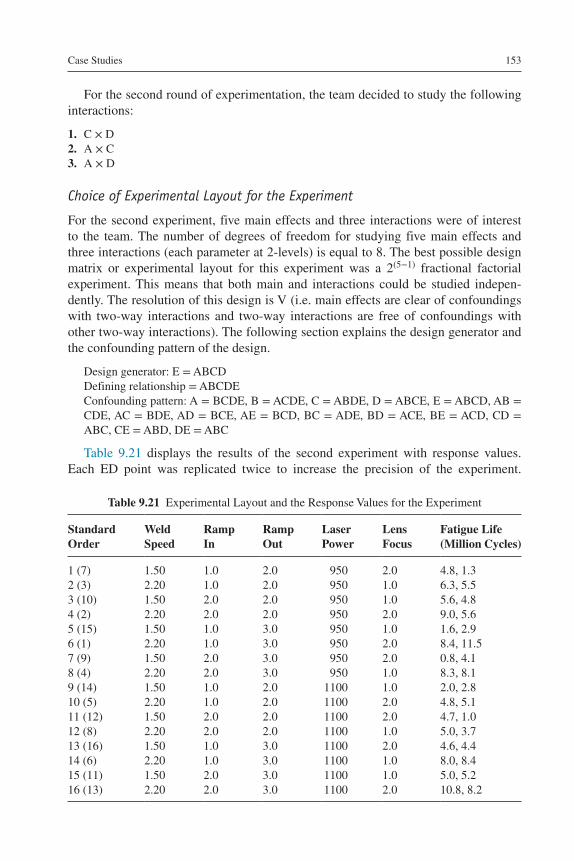
Case Studies 153
For the second round of experimentation, the team decided to study the following interactions:
1. C × D2. A × C3. A × D
Choice of Experimental Layout for the Experiment
For the second experiment, five main effects and three interactions were of interest to the team. The number of degrees of freedom for studying five main effects and three interactions (each parameter at 2-levels) is equal to 8. The best possible design matrix or experimental layout for this experiment was a 2(5−1) fractional factorial experiment. This means that both main and interactions could be studied indepen-dently. The resolution of this design is V (i.e. main effects are clear of confoundings with two-way interactions and two-way interactions are free of confoundings with other two-way interactions). The following section explains the design generator and the confounding pattern of the design.
Design generator: E = ABCDDefining relationship = ABCDEConfounding pattern: A = BCDE, B = ACDE, C = ABDE, D = ABCE, E = ABCD, AB = CDE, AC = BDE, AD = BCE, AE = BCD, BC = ADE, BD = ACE, BE = ACD, CD = ABC, CE = ABD, DE = ABC
Table 9.21 displays the results of the second experiment with response values. Each ED point was replicated twice to increase the precision of the experiment.
Table 9.21 Experimental Layout and the Response Values for the Experiment
Standard Order
Weld Speed
Ramp In
Ramp Out
Laser Power
Lens Focus
Fatigue Life (Million Cycles)
1 (7) 1.50 1.0 2.0 950 2.0 4.8, 1.32 (3) 2.20 1.0 2.0 950 1.0 6.3, 5.53 (10) 1.50 2.0 2.0 950 1.0 5.6, 4.84 (2) 2.20 2.0 2.0 950 2.0 9.0, 5.65 (15) 1.50 1.0 3.0 950 1.0 1.6, 2.96 (1) 2.20 1.0 3.0 950 2.0 8.4, 11.57 (9) 1.50 2.0 3.0 950 2.0 0.8, 4.18 (4) 2.20 2.0 3.0 950 1.0 8.3, 8.19 (14) 1.50 1.0 2.0 1100 1.0 2.0, 2.810 (5) 2.20 1.0 2.0 1100 2.0 4.8, 5.111 (12) 1.50 2.0 2.0 1100 2.0 4.7, 1.012 (8) 2.20 2.0 2.0 1100 1.0 5.0, 3.713 (16) 1.50 1.0 3.0 1100 2.0 4.6, 4.414 (6) 2.20 1.0 3.0 1100 1.0 8.0, 8.415 (11) 1.50 2.0 3.0 1100 1.0 5.0, 5.216 (13) 2.20 2.0 3.0 1100 2.0 10.8, 8.2

Design of Experiments for Engineers and Scientists154
Moreover, the trial condition was also randomised to minimise the effect of bias induced into the experiment.
Statistical Analysis and Interpretation
In order to meet the objectives set at the outset of the project, it was important to per-form statistical analysis of the data generated from the experiment. If the experiment was planned, designed, conducted and analysed correctly, then statistical analysis would provide sound and valid conclusions. The first step was to estimate the main and interaction effects of interest. Table 9.22 presents the table of effects and regres-sion coefficients.
The identification of active and real effects is obtained with the help of Pareto and main effect plots. Figures 9.23 and 9.24 present these. Figures 9.23 and 9.24 indi-cate that two main effects (WS and RO) and two interaction effects (WS × RO) and (RO × LP) are found to be statistically significant at 5% significance level. Here sig-nificance level is the risk of saying that a factor effect or an interaction is significant
Table 9.22 Table of Effects and Regression Coefficients
Term Effect Coefficient
A (WS) 3.819 1.595B (RI) 0.469 0.235C (RO) 1.769 0.885D (LP) −0.306 −0.153E (LF) 0.369 0.185A × C (WS × RO) 1.569 0.785A × D (WS × LP) −0.781 −0.391C × D (RO × LP) 1.419 0.709
WS RI RO LP LF3.4
4.4
5.4
6.4
7.41.5 2.2 1 2 2 3 950 1100 1 2
Mea
n lif
e
Figure 9.23 Main effects plot for the experiment.

Case Studies 155
when in fact it is not. The main effect and Pareto plots indicate that weld speed is the most active factor effect, followed by ramp out. The interaction between ramp out and laser power is shown in Figure 9.25. The interaction plot shows that life increases when both laser power and ramp out are at high level.
It is quite interesting to note that although laser power on its own has very little impact on the life of core tubes, its effect on life is dependent on ramp out (Figure 9.25). In order to observe the effect of three factors on the mean life of core tubes, a cube plot is constructed (Figure 9.26). It is quite apparent in the cube plot that a high level of weld speed will yield a higher life. Similarly, it is fair to say that life increases with increase in ramp out.
The next step in the analysis was to identify the factors which influence fatigue life variability (Sirvanci and Durmaz, 1993). To analyse variability, SD was
0 1 2 3 4 5 6 7
D
E
B
AD
CD
AC
C
A
A: WSB: RIC: ROD: LPE: LF
Figure 9.24 Pareto plot of effects affecting mean life.
950 1100
3.8
4.8
5.8
6.8
LP
23
RO
Mea
n lif
e
Figure 9.25 Interaction plot – ramp out × laser power.

Design of Experiments for Engineers and Scientists156
calculated at each ED point. As log(SD) values will tend to be normally distributed, a log transformation on SD values was essential. Table 9.23 displays the log(SD) val-ues corresponding to each experimental trial condition. Due to insufficient degrees of freedom for the error term, it was decided to pool those effects with low magnitude. The Pareto chart (Figure 9.27) shows that the main effects lens position and laser power are significant at 5% significance level. Similarly, it was also found that the interactions between lens focus and ramp in and laser power and ramp in were sig-nificant. Similar results can be obtained using analytical tools such as ANOVA. For more information on the ANOVA, readers are encouraged to refer to Montgomery’s book, Design and Analysis of Experiments. Having identified the process parameters
6.600
4.650
9.075
8.850
4.125
2.625
2.350
4.800
1.5 2.2WS
RO
LP
2
3
950
1100
Figure 9.26 Cube plot of factors with mean life of core tubes.
Table 9.23 Table of log(SD) Values
Trial No. log(SD)
1 0.3942 −0.2473 −0.2474 0.3815 −0.0376 0.3417 0.3688 −0.8519 −0.247
10 −0.67411 0.41812 −0.03713 −0.85114 −0.54815 −0.85116 0.264

Case Studies 157
which influence the mean and variability, the next stage was to determine the opti-mal process parameter settings that would maximise the core tube life with minimum variability.
Determination of the Optimal Process Parameter Settings
The selection of optimal settings of the process parameters depends a great deal on the objectives to be achieved from the experiment and the nature of the problem to be tackled. For the present study, the engineering team within the company want to discover the settings of the key process parameters that will not only maximise the core tube mean life but also reduce variability in core tube life so that more consist-ent and reliable products can be produced by the manufacturer (Montgomery, 1992).
To identify the process parameter settings which maximise the life, it was impor-tant to select the best levels of those parameters which yield maximum core tube life. This information can be easily generated from the main effects plot (Figure 9.23). The interaction plot between ramp out (C) and laser power (D) suggests that (Figure 9.25) the core tube life is maximum when the laser power is set at its high level. Therefore, the optimal settings for maximising the core tube life are as follows:
Weld speed (A) – level 2 (2.2 rev./s)Ramp out (C) – level 2 (3.0 s)Laser power (D) – level 2 (1100 W)
In essence, the maximum core tube life was achieved only when all of the above process parameters were kept at high levels.
In order to determine the best levels of process parameters which yield mini-mum variability, it was decided to construct a main effects plot on variability (using log(SD) as the response of interest). Figure 9.28 presents the main effects plot of process parameters for variability (log(SD) as the response).
0 1 2 3 4
A
CD
B
AD
AC
C
DE
D
BD
BE
E
A: WSB: RIC: ROD: LPE: LF
Figure 9.27 Pareto plot of effects influencing variability.

Design of Experiments for Engineers and Scientists158
The optimal settings for the significant process parameters which influence vari-ability in core tube life are as follows:
Ramp in (B) – Level 1 (1 sec.)Laser power (D) – Level 2 (1100 W)Lens focus (E) – Level 1 (Position 1)
As there was no trade-off in the levels of the process parameters, the final settings were determined by combining the above two. The final optimal condition is there-fore given by
Weld speed (A) – Level 2 (2.2 rev./s)Ramp in (B) – Level 1 (1 sec.)Ramp out (C) – Level 2 (3.0 s)Laser power (D) – Level 2 (1100 W)Lens focus (E) – Level 1 (Position 1)
Confirmation Trials
Confirmation trials were performed in order to verify the results of the analysis. Five samples were produced at the optimal condition of the process. The mean life of the core tubes and tube life variance were 10.25 and 0.551, as opposed to 6.75 and 1.6 at the normal production settings in the company. This showed an improvement of over 50% in the life of the core tubes and a 65% reduction in core tube life variability.
Significance of the Study
Due to the significant reduction in process variability, the costs due to poor quality such as scrap, rework, replacement, re-test, etc. were reduced by over 20%. This shows a dramatic improvement in the performance of the process and thereby more consistent and higher-quality core tubes could be produced using the opti-mised process. The engineering team within the company are now well aware of the do’s and don’ts of ED. Moreover, the awareness of DOE that has been estab-lished within the organisation has built confidence among the engineers and among
WS RI RO LP LF
1.5 2.2 1 2 2 3 950 1100 1 2
–0.38
–0.26
–0.14
–0.02
0.10
log
(SD
)
Figure 9.28 Main effects plot on variability (log(SD)).

Case Studies 159
front-line workers in other areas facing similar difficulties. The author believes that it is important to teach a case study of this nature in order to learn the common pitfalls when applying DOE to a specific problem. The experiment also helped the engineering team within the company to understand not only the fundamental mis-takes they were making but also the key features of making an industrial experiment a successful event.
9.2.8 Optimisation of a Spot Welding Process Using DOE
This case study presents the application of DOE to a spot welding process in order to discover the key process parameters which influence the tensile strength of welded joints. Spot welding is the most commonly used form of resistance welding. The metal to be joined is placed between two electrodes, pressure applied and a current turned on. The electrodes pass an electric current through the work pieces. As the welding current is passed through the material via the electrodes, heat is generated, mainly in the material at the interface between the sheets. As time progresses, the heating effect creates a molten pool at the joint interface which is contained by the pressure at the electrode tip. Once the welding current is switched off, the molten pool cools under the continued pressure of the electrodes to produce a weld nugget.
The heat generated depends on the electrical resistance and thermal conductivity of the metal, and the time at which the current is applied. The electrodes are held under a controlled pressure or force during the welding process. The amount of pres-sure affects the resistance across the interfaces between the work pieces and the electrodes. If the applied pressure is too low, weld splash (a common defect in spot resistance welding) may occur.
There are three stages to the welding cycle: squeeze time, weld time and hold time. The squeeze time is the period from when the pressure is applied until the cur-rent is turned on. The weld time is the duration of the current flow. If the weld cur-rent is high, this may again lead to weld splash. The hold time is the time for which the metal is held together after the current is stopped.
As part of initial investigation and because no experiments have been performed on the spot welding machine before, the engineers within the company were more interested in understanding the process itself, including the key welding process parameters, which affect the mean strength of the weld, and the process parameters, which affect the variability in weld strength.
The following objectives therefore were set by a team of people within the com-pany consisting of quality improvement engineers, a process manager, two operators, a production engineer and a DOE facilitator who is an expert in the subject matter. The objectives of the experiment were as follows:
1. to identify the key welding process parameters which influence the strength of the weld2. to identify the key welding process parameters which influence variability in weld strength.
Table 9.24 presents the list of process parameters along with their levels used for the experiment. As part of the initial investigation, it was decided to study the process parameters at 2-levels. Owing to the non-disclosure agreement between the company and the author, certain information relating to the case study (process

Design of Experiments for Engineers and Scientists160
parameters, levels and original data) cannot be revealed. However, the data have not been manipulated or modified as a consequence of this agreement.
Interactions of Interest
Further to a thorough brainstorming session, the team has identified the following interactions of interest:
a. A × Bb. B × Dc. C × Dd. D × E
The quality characteristic of interest for this study was weld strength measured in kilograms. Having identified the quality characteristic and the list of process param-eters, the next step was to select an appropriate design matrix for the experiment. The design matrix shows all the possible combinations of process parameters at their respective levels. The choice of design matrix or experimental layout is based on the degrees of freedom required for studying the main and interaction effects (Bullington et al., 1993). The total degrees of freedom required for studying five main effects and four interaction effects is equal to nine. A 2(5−1) fractional factorial design was selected to study all the main and interaction effects stated above. The degrees of freedom associated with this design is 15 (i.e. 16−1).
In order to minimise the effect of noise factors induced into the experiment, each trial condition was randomised. Randomisation is a process of performing experimental tri-als in a random order in which they are logically listed. The idea is to evenly distribute the effect of noise (factors which are difficult or expensive to control under standard production conditions) across the total number of experimental trials. Moreover, each design point was replicated five times to improve the efficiency of experimentation. The purpose of replication is to capture variation due to machine set-up, operator error, etc. Moreover, replications generally provide estimates of error variability for the factors (or process parameters). Table 9.25 illustrates the results of the experiment.
Statistical Analysis of Experimental Results
Statistical analysis and interpretation of results are imperative steps for DOE to meet the objectives of the experiment. A well-planned and well-designed experiment
Table 9.24 List of Process Parameters Used for the Experiment
Process Parameter Label Low-Level Setting
High-Level Setting
Stroke distance A −1 1Weld time B −1 1Electrode diameter C −1 1Welding current D −1 1Electrode pressure E −1 1

Case Studies 161
will provide effective and statistically valid conclusions. The first step in this par-ticular analysis was to identify the factors and interactions which influence the mean weld strength. The results of the analysis are shown in Figure 9.29. The Pareto plot (Figure 9.29) shows that main effects D (welding current) and E (electrode pressure) have a significant influence on mean weld strength. Moreover, two interactions A × B (stroke distance × weld time) and B × D (weld time × welding current) are also
Table 9.25 Results of the Experiment
Run A B C D E Mean Weld Strength
1 −1 −1 −1 −1 −1 5.42 1 −1 −1 −1 1 20.43 −1 1 −1 −1 1 243.04 1 1 −1 −1 −1 109.05 −1 −1 1 −1 −1 486 1 −1 1 −1 1 1047 −1 1 1 −1 1 23.68 1 1 1 −1 −1 3.409 −1 −1 −1 1 −1 763
10 1 −1 −1 1 1 75011 −1 1 −1 1 1 55312 1 1 −1 1 −1 27913 −1 −1 1 1 −1 46214 1 −1 1 1 1 61015 −1 1 1 1 1 74716 1 1 1 1 −1 576
20100
D
AB
E
BD
A
DE
C
CD
B
A: Stroke distanceB: Weld timeC: Electrode diameterD: Welding currentE: Electrode pressure
Figure 9.29 Pareto plot of main and interaction effects from the experiment.

Design of Experiments for Engineers and Scientists162
found to be statistically significant. Main effects A, C and B did not have any influ-ence on the mean weld strength.
In order to analyse the strength of the interaction among the process parameters stroke distance, weld time and welding current, it was decided to construct interac-tion graphs (Figures 9.30 and 9.31).
Figure 9.30 shows that high weld time and low stroke distance yield the high-est weld strength, whereas high weld time and high stroke distance yield the low-est weld strength. Similarly, Figure 9.31 indicates that high welding current and low weld time yield the highest weld strength. Here there is a trade-off in the selection of factor levels for weld time. However, further studies showed that the combination of high weld time and high welding current produces the highest weld strength.
1–1
390
340
290
240
Weld time
–11
Stroke distanceM
ean
wel
d st
reng
th
Figure 9.30 Interaction graph for weld time and stroke distance.
1–1
650
550
450
350
250
150
50
Welding current
–1
1
Weld time
Mea
n w
eld
stre
ngth
Figure 9.31 Interaction graph for welding current and weld time.

Case Studies 163
One of the assumptions experimenters generally make in the analysis part is that the data come from a normal population. In order to verify that the data follow a normal distribution in this instance, it was decided to construct an NPP of residu-als (residual = observed value − predicted value). Figure 9.32 presents an NPP of residuals which clearly indicates that all the points on the plot come close to forming a straight line. This implies that the data are fairly normal.
The next step in the analysis was to identify the key process parameters which affect variability in weld strength. To analyse variability, SD was calculated at each experimental trial condition (Logothetis and Wynn, 1989). As ln(SD) values will tend to be normally distributed, a log transformation was carried out on the data. The results are given in Table 9.26.
–200 –100 0 100 200
–2
–1
0
1
2
Nor
mal
sco
re
Residual
Figure 9.32 NPP of residuals.
Table 9.26 ln(SD) Values from the Experiment
Trial No. ln(SD)
1 1.0862 2.9613 3.6424 3.7135 4.0086 3.4817 3.3798 1.3299 4.011
10 3.37911 3.93112 4.93713 3.64614 3.56015 4.00016 4.070
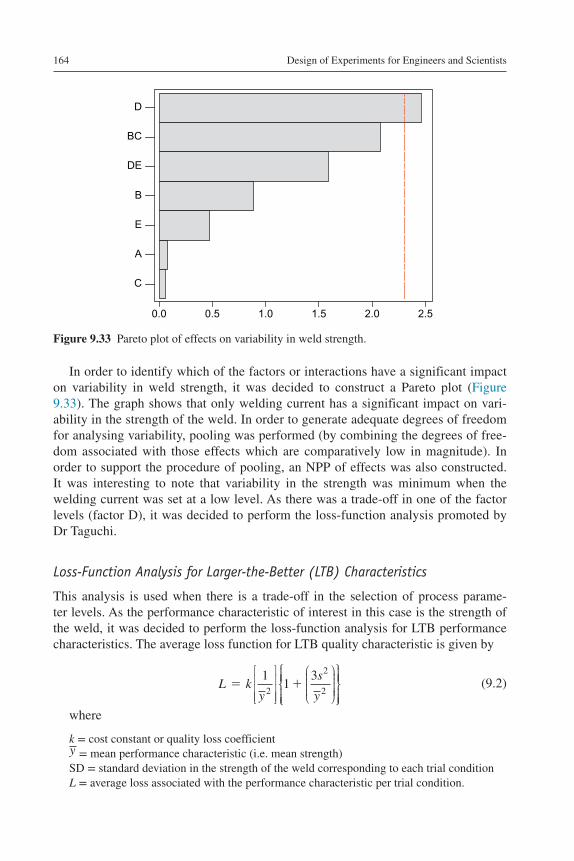
Design of Experiments for Engineers and Scientists164
In order to identify which of the factors or interactions have a significant impact on variability in weld strength, it was decided to construct a Pareto plot (Figure 9.33). The graph shows that only welding current has a significant impact on vari-ability in the strength of the weld. In order to generate adequate degrees of freedom for analysing variability, pooling was performed (by combining the degrees of free-dom associated with those effects which are comparatively low in magnitude). In order to support the procedure of pooling, an NPP of effects was also constructed. It was interesting to note that variability in the strength was minimum when the welding current was set at a low level. As there was a trade-off in one of the factor levels (factor D), it was decided to perform the loss-function analysis promoted by Dr Taguchi.
Loss-Function Analysis for Larger-the-Better (LTB) Characteristics
This analysis is used when there is a trade-off in the selection of process parame-ter levels. As the performance characteristic of interest in this case is the strength of the weld, it was decided to perform the loss-function analysis for LTB performance characteristics. The average loss function for LTB quality characteristic is given by
L ky
s
y
11
32
2
2
where
k = cost constant or quality loss coefficienty = mean performance characteristic (i.e. mean strength)SD = standard deviation in the strength of the weld corresponding to each trial conditionL = average loss associated with the performance characteristic per trial condition.
(9.2)
0.0 0.5 1.0 1.5 2.0 2.5
C
A
E
B
DE
BC
D
Figure 9.33 Pareto plot of effects on variability in weld strength.

Case Studies 165
Equation (9.2) is applied to all 16 trial conditions. It was found that trial condi-tion 10 yields minimum loss. For trial condition 10, factor D was set at high level and therefore the high-level setting for D was chosen for the model development and prediction of weld strength.
Significance of the Study
The purpose of this paper is to illustrate an application of DOE to a spot welding process. The objectives of the experiment in this study were twofold. The first objec-tive was to identify the critical welding process parameters which influence the strength of the weld. The second objective was to identify the process parameters which affect variability in the weld strength. A trade-off in one of the factor levels (factor D) was observed. This problem was rectified with the use of Taguchi’s loss-function analysis. The strength of the weld was increased by around 25%. The next phase of the research is to perform more advanced methods such as RSM by adding centre points and axial points to the current design. The results of the experiment have stimulated the engineering team within the company to extend the applications of DOE in other core processes for performance improvement and variability reduc-tion activities.
9.2.9 DOE Applied to a Fizz-Flop Experiment
The purpose of this experiment was to determine which factors influence the mean response and variation of response of an effervescent pain relief tablet (hereafter referred to as a tablet) being dissolved in a liquid. The time taken to completely dis-solve one tablet will be measured and recorded in seconds. This experiment was given out to a group of students pursuing a Masters Programme on Lean Six Sigma at the University of Strathclyde, Scotland.
By means of a brainstorming session the team (consists of five students) consid-ered potential factors and how they might affect the time needed to dissolve a sin-gle tablet. As this is a commercially available product which is taken orally, process parameters were limited to those which would not affect consumer safety. As the team members had no previous experience of the process under investigation, we used six tablets to help with the brainstorming. Figure 9.34 illustrates the Cause and Effect diagram produced during the brainstorming. Team discussions led to further consideration of the factors which were considered to affect the response. Table 9.27 gives the final output which was to be used in the ED. This included the following information:
● Factor: process parameters selected to be considered during the experiment● Possible levels: levels selected to give as wide a scope as reasonably possible● Group thinking: the thoughts of the team with regards to factors and why specific levels
were chosen● Considered for experiment: the 2-levels chosen for each factor● Considered as key factor: the thoughts of the team prior to carrying out the experiments as
to whether a particular factor would influence the response.

Design of Experiments for Engineers and Scientists166
Tim
e to
dis
solv
eta
ble
t
Man
Met
ho
d
Mac
hin
eM
ater
ial
Tra
inin
g
No.
of t
eam
mem
bers
Stir
ring:
yes,
no
Spe
ed o
f stir
ring:
slow
, fas
t
Ope
ratio
nal S
eque
nce:
tabl
et o
r liq
uid
first
Siz
e of
stir
rer
Typ
e of
stir
rer
Vol
ume
of li
quid
Tem
pera
ture
of l
iqui
d:ho
t, co
ld, l
uke
war
m
Tab
let f
orm
:w
hole
, hal
ves,
qua
rter
s, c
rush
ed
Typ
e of
liqu
id :
wat
er, D
iet C
oke,
Die
t Lem
eona
de, D
iet I
rn B
ru
Cup
type
:gl
ass,
pol
ysty
rene
, pla
stic
, pap
er
Siz
e of
cup
: sm
all,
larg
e
Sto
pwat
ch:
man
ual,
digi
tal
The
rmom
eter
:di
gita
l, m
anua
l, la
ser
Liqu
id h
eatin
g:po
t/mic
row
ave
Liqu
id c
oolin
g:re
frig
erat
e, fr
eeze
r, ta
p
En
viro
nm
ent
Exp
erim
ent
loca
tion
Tea
m s
afet
y
Liqu
id d
ilutio
n :
liqui
d on
ly, l
iqui
d di
lute
d in
wat
er
Met
hod
of s
tirrin
g:au
to, m
anua
l
Fig
ure
9.34
Cau
se a
nd E
ffec
t dia
gram
.

Case Studies 167
Table 9.27 Final Output from Brainstorming
Factor Possible Levels
Group Thinking Chosen for Experiment
Considered as Key Factor in Response
Type of cup Paper No chemical reaction with cup material is expected in either case. Possible difference in heat loss characteristics, particularly with hot water. Plastic and Glass were chosen as these allowed good visibility of the table during dissolving process
✗ NoPlastic ✓
Polystyrene ✗
Glass ✓
Size of cup ½ pint The size of cup is not expected to affect the response but must be able to hold the specified volume and temperature of liquid
✓ Nopint ✓
Volume of liquid
4 fl. oz. 4 fl. oz. is the supplier recommended volume. Additional volume may allow a greater chemical reaction in the creation of carbon dioxide and therefore speed up the dissolving process
✓ Possible8 fl. oz. ✓
Liquid temperature
Cold (40°F) The dissolving process is likely to be affected by significant change in water temperature, with higher temperatures speeding up the time to dissolve a tablet
✓ YesHot (175°F) ✓
Type of liquid
Water The supplier recommends using water as the solvent. Using a carbonated soft drink as an additive could have two effects: (1) lower pH value which may speed up response time of the chemical reaction and (2) increase carbon dioxide content which may increase time to dissolve a tablet Diet Lemonade was chosen as it was found to be easier to view the tablet during the experiments
✓ YesDiet Lemonade ✓
Diet Irn Bru ✗
Diet Coke ✗
(Continued)

Design of Experiments for Engineers and Scientists168
Hypotheses
Prior to the experiment, hypotheses were considered by every team member regard-ing which factors would make the tablet dissolve the fastest, as this would provide evidence as to what potential outcomes were perceived to happen. The hypotheses perceived prior to experimentation were the following:
Mr A – hot water and stirring whilst dissolvingMr B – hot water and the tablet being crushed prior to being put in waterMs C – cold water and a wide-rimmed cupMs D – hot water and a glassMr E – cold sparkling water with salt added to the solution.
The team consisted of four people who performed all aspects of the experiment without additional resources. Table 9.28 lists materials and resources that were used during the experiment.
Experimental Plan
The output of the brainstorming session suggested eight possible factors which could affect the response (i.e. time to dissolve tablet). It was decided to study each factor at 2-levels in the initial part of the investigation. For an FFE, this would require 256 experi-ments or trials (e.g. 28 = 256). As the first objective of the experiment was to determine
Table 9.27 Final Output from Brainstorming
Factor Possible Levels
Group Thinking Chosen for Experiment
Considered as Key Factor in Response
Tablet size Full The size will affect the surface area of the tablet exposed to the solvent. The greater the initial surface area, the faster the response is likely to be. Crushed was ruled out as it was extremely difficult to record when the dissolving process had finished. Full tablets and Quarters were chosen to provide a suitable scope
✓ YesHalves ✗
Quarters ✓
Crushed ✗
Operational sequence
Liquid then tablet
The dissolving process may be affected by the impact of pouring liquid over a tablet or dropping a tablet into the liquid
✓ No
Tablet then liquid
✓
Stirring No Once the chemical reaction starts, the act of stirring is likely to speed up the time for a tablet to dissolve
✓ YesYes ✓
Table 9.27 (Continued)

Case Studies 169
the main factors which affected the mean response, the team decided to carry out a screening experiment. Furthermore, as the second objective was to determine which fac-tors affected the variability of response, it was decided to replicate each trial condition. Based on the these objectives, the limited availability of tablets, the relatively low cost of the materials and the time required to carry out the experiments, the team decided to carry out a PB-12 trial experiment with two replicates. It was also decided that the exper-iments would be randomised in order to distribute the random effects of noise (if any).
A PB-12 experiment allows for up to 11 factors at 2-levels to be considered and offers 11 degrees of freedom. As we were only considering eight factors, this allowed us to create 3 degrees of freedom for the error term.
The measurement system to be used by the team was agreed and consisted mainly of the following:
● liquid volume measured using a measuring jug● liquid temperature measured by an analogue thermometer● time to dissolve (response) measured by a stopwatch.
As these were all manual and open to judgement and error, the capability and sta-bility of the measurement system could not be guaranteed. Table 9.29 gives the final list of factors, with their low and high levels, to be used during the experimentation.
The following information was entered into Minitab along with the following:
● number of experiments = 12● experimental method = Plackett–Burman● replicates = 2● randomisation = Yes
Table 9.30 presents the P–B experimental layout used for the experiment.
Table 9.28 List of Available Materials
Description Quantity Purpose/Comment
Measuring jug (0–16 fl. oz.)
1 To calibrate the amount of liquid used in each experiment
Thermometer (manual) 1 To measure the liquid temperatureStopwatch 1 To measure the time to dissolve the tablet during each
experimentEffervescent pain relief tablets
30 6× tablets were used for pre-experiment investigation24× tablets were used during the experiments
Plastic cup (½ pint) 6 To hold hot and cold liquids and have the capacity to hold the desired volume levelsPlastic cup (pint) 6
Glass cup (½ pint) 6Glass cup (pint) 6Diet Lemonade 6 L Liquids to be chilled to 40°F and heated to 175°F based on EDWater 6 LPan 1 To heat liquid for high-level temperature experimentsMeasuring spoon (1 tsp.)
1 To stir solution for appropriate experiments

Design of Experiments for Engineers and Scientists170
Table 9.29 List of Factors and Their Respective Levels
Factor ID Description Low Level (−) High Level (+)
A Type of cup Plastic GlassB Cup size ½ pint PintC Volume of liquid 4 fl. oz. 8 fl. oz.D Liquid temperature 40°F 175°FE Type of liquid Water Diet LemonadeF Tablet size Quarters FullG Operational sequence Tablet then liquid Liquid then tabletH Stirring No Yes
Table 9.30 Experimental Layout for the Fizz-Flop Experiment
Exp. No. Factor
A B C D E F G H
1 − + + − + − − −2 − + + + − + + −3 + − + + − + − −4 + − − − + + + −5 − + + + − + + −6 − − − + + + − +7 − − − + + + − +8 + + + − + + − +9 + + − + − − − +
10 + + − + − − − +11 − − + + + − + +12 − + + − + − − −13 + + − + + − + −14 − + − − − + + +15 + + + − + + − +16 + − + + − + − −17 + − − − + + + −18 − − − − − − − −19 + + − + + − + −20 + − + − − − + +21 + − + − − − + +22 − + − − − + + +23 − − + + + − + +24 − − − − − − − −
Case Studies 171
Execution of Experiment
To minimise the effect of manual error during the experiments, the following approach was taken:
● Person 1:prepared the cup and liquid for each experiment; added tablet to experiments with in the order of Liquid then Tablet
● Person 2:stirred the solution for appropriate experiments; measured time to dissolve each tablet (response) with stopwatch.
This ensured that Person 1 would be responsible for the measurement of the two quantitative characteristics (liquid volume and temperature) and Person 2 would be responsible for the measurement of the response time. This was expected to reduce the level of operator error, as this was not considered a key factor in our experiments.
The experiments were set up, executed and recorded on an individual basis, based on the randomised design stated by Minitab.
The 40°F liquids were refrigerated and the 175°F liquids were heated in a pan in advance of the experiments.
Data Collection, Analysis and Interpretation
Data CollectionThe 24 experiments were conducted and the responses (time to dissolve each tablet) were recorded as given in Table 9.31.
Analysis of DataThe first part of the analysis was to determine which of the factors in the experi-ment had the highest impact on the response. For simplicity reasons, it was decided to construct a main effects plot (Figure 9.35). Figure 9.35 clearly shows that all factors apart from liquid temperature do not greatly affect the response. Obviously, the graph shows that when liquid temperature increased from 40°F to 175°F, the time taken for the tablet to dissolve is reduced significantly. In order to determine the statistical significance, it was decided to use both a normal plot and a Pareto plot so that valid and robust conclusions could be drawn from the experi-ment. Both plots (Figure 9.36 and Figure 9.37) suggested that liquid temperature is the only factor which appeared to be statistically significant at the 5% signifi-cance level.
The second phase of the analysis was focused on the factors which influence the response variability, that is, variability in the time taken for the tablets to dissolve. In order to analyse variability, we have computed the SD at each ED point (Table 9.31). An NPP of effects for variability, In(SD), was constructed. The graph (Figure 9.38) has shown that both liquid temperature and liquid type have an impact on the response variability. It was also observed from further analysis that higher liquid temperature gave less variability in response and Diet Lemonade provided the team with minimal variability in response compared to water.

Design of Experiments for Engineers and Scientists172
Tabl
e 9.
31 R
esul
ts o
f th
e P–
B 1
2 E
xper
imen
t with
Res
pons
e V
alue
s
Run
O
rder
R
1/R
2
AB
CD
EF
GH
Res
pons
e (s
)A
naly
sis
Cup
T
ype
Cup
Si
zeV
olum
e of
Liq
uid
(fl.o
z.)
Liq
uid
Tem
pera
ture
(°
F)
Liq
uid
Typ
eTa
blet
Si
zeO
pera
tion
al
Sequ
ence
Stir
ring
R1
R2
Mea
nSD
ln(S
D)
1/12
Plas
tic1
840
Die
t Lem
onad
eQ
uart
ers
Tabl
et th
en li
quid
No
109.
8490
.00
99.9
214
.03
2.64
2/5
Plas
tic1
817
5W
ater
Who
leL
iqui
d th
en ta
blet
No
19.9
424
.69
22.3
23.
361.
213/
16G
lass
0.5
817
5W
ater
Who
leTa
blet
then
liqu
idN
o19
.34
22.0
420
.69
1.91
0.65
4/17
Gla
ss0.
54
40D
iet L
emon
ade
Who
leL
iqui
d th
en ta
blet
No
91.5
076
.97
84.2
410
.27
2.33
6/7
Plas
tic0.
54
175
Die
t Lem
onad
eW
hole
Tabl
et th
en li
quid
Yes
16.0
917
.56
16.8
31.
040.
048/
15G
lass
18
40D
iet L
emon
ade
Who
leTa
blet
then
liqu
idY
es92
.75
70.1
081
.43
16.0
22.
779/
10G
lass
14
175
Wat
erQ
uart
ers
Tabl
et th
en li
quid
Yes
17.7
814
.94
16.3
62.
010.
7011
/23
Plas
tic0.
58
175
Die
t Lem
onad
eQ
uart
ers
Liq
uid
then
tabl
etY
es17
.37
16.4
116
.89
0.68
−0.
3913
/19
Gla
ss1
417
5D
iet L
emon
ade
Qua
rter
sL
iqui
d th
en ta
blet
No
15.1
016
.19
15.6
50.
77−
0.26
14/2
2Pl
astic
14
40W
ater
Who
leL
iqui
d th
en ta
blet
Yes
101.
6065
.32
83.4
625
.65
3.24
18/2
4Pl
astic
0.5
440
Wat
erQ
uart
ers
Tabl
et th
en li
quid
No
111.
4179
.38
95.4
022
.65
3.12
20/2
1G
lass
0.5
840
Wat
erQ
uart
ers
Liq
uid
then
tabl
etY
es81
.00
56.6
268
.81
17.2
42.
85

Case Studies 173
Experimental ConclusionsFrom the experiments carried out and analysis of the results, the following conclu-sions were drawn by the team:
● Only factor D (liquid temperature) has a significant effect on the mean time to dissolve a tablet.
● Factor D (liquid temperature) and factor E (liquid type) have a significant effect on the variability of time needed to dissolve a tablet.
GlassPlastic 1.00.5 84
17540 Diet lemonadeWater WholeQuarters
Liquid then tabletTablet then liquid
90
60
30
90
60
30
90
60
30
YesNo
Cup type
Mea
n
Cup size Volume of liquid
Liquid temperature Liquid type Tablet size
Operational sequence Stirring
Main effects plot for responsesData means
Figure 9.35 Main effects plot for the Fizz-Flop experiment.
Volume of liquid
Tablet size
Liquid type
Cup size
Operational sequence
Cup type
Stirring
Liquid temperature
14121086420
Ter
m
Standardised effect
2.13
Pareto chart of the standardised effects(response is responses, alpha = 0.05)
Figure 9.36 Pareto plot of the effects for the Fizz-Flop experiment.

Design of Experiments for Engineers and Scientists174
● All other factors can be set at economical or customer-defined levels as they do not influ-ence either the mean time or variability of time needed to dissolve a tablet.
● Interactions between factors were not considered and could be included in further rounds of experimentation.
Key Lessons Learned
Mr A: This exercise confirmed my view that DOE is an extremely powerful tool within Six Sigma. We carried out only a basic screening exercise but I will pursue
0–4–8–12–16
99
95
90
80706050403020
10
5
1
Standardised effect
Per
cen
t
Not significantSignificant
Effect type
Liquid temperature
Normal plot of the standardised effects(response is responses, alpha = 0.05)
Figure 9.37 NPP of effects (mean response).
99
95
90
80706050403020
10
5
1
Standardised effect
Per
cen
t
Liquid Temperature
Normal plot of the standardised effects(Response is ln of standard deviation, alpha = 0.05)
0–5–10–15–20–25
Liquid type
Liquid temperature
Not significantSignificant
Effect type
Figure 9.38 NPP of effects (response variability).
Case Studies 175
further opportunities to learn and practice further DOE with a view to expanding my knowledge and understanding and introducing it within my workplace.
Mr B: DOE was an eye-opener for me. It encouraged me to approach the experi-ments in a more scientific manner. As an engineer, it has also motivated me to avoid making judgments based on the OFAT approach to experimentation. I feel my hypothesis was really out of place; the lesson here was to study more about the actual process that you are going to experiment on. The beauty of this technique was its foundations and solutions based on data and facts. Moreover, this assignment has been a really interesting team bonding experience, full of enthusiasm and shared knowledge.
Ms C: The use of brainstorming was very important. I believe that had this been an individual exercise a lot of factors would never have come to light.
Understanding and interpreting data and statistics have proved to be a very impor-tant aspect in the use of DOE. I would have expected stirring to have a greater effect on the experiment and the result achieved was surprising which suggests that gut instinct is not always correct. This experiment also highlighted how time-consum-ing and complex experimentation can be, even in a very simple experiment, which explains why companies are so hesitant to conduct designed experiments and also exemplifies how beneficial DOE can be in reducing the size of the experiment but still allowing us to understand the process more efficiently and effectively.
Ms D: ED appears complicated and requires a good grasp of basic statistics in order to successfully apply this technique in real-world scenarios. It is easy to see why it is used so little in industry. Partial knowledge could lead to misinterpreta-tion of results or incorrectly applying the method, leading to frustration and even avoidance of the technique. In my opinion a good coach is vital in order to steer you through the potential pitfalls.
I believe once you have completed three to four experiments and have gained experience and confidence this would be a powerful tool. At this particular time I believe I require further coaching, and would benefit from being involved in a complete experiment (screening, characterisation and optimisation) with a good practitioner.
Using a good screening experimentation such as Plackett–Burman, one could save hundreds of pounds and time associated with experimentation. I was unaware of this technique before and the knowledge gained from this experiment will benefit me greatly in the future.
Mr E – This was an extremely interesting experiment to me as the outcome was different to the original thinking of many in the group. This showed how assump-tions can be incorrect from the outset. Team working is the key to achieve great results. When everybody has clear roles and responsibilities the team functions more effectively and achieves the goal in less time than expected.
Significance of the Study
Team work was found to be vital. This exercise has confirmed the importance of having the right people in attendance at the initial brainstorming. Even carrying out

Design of Experiments for Engineers and Scientists176
a basic screening experiment highlighted the benefits a knowledgeable team would bring. We had no prior knowledge of the product or process under investigation and may have missed some important factors, or deemed them to be unimportant. Our chosen DOE approach did not consider factor interaction and we did not have enough tablets to carry out further testing. We would welcome the opportunity to be involved in further experimentation, particularly for process characterisation and optimisation.
9.2.10 DOE Applied to a Higher Education Context
This case study was executed to remove the myth that DOE is purely confined to manufacturing processes. This case study basically encompasses delivery of a course to both undergraduate and postgraduate students in the Faculty of Engineering at a UK-based university. One of the key outputs of teaching is how well the students have learned the topic and how useful and relevant the topics and contents of the course are to them. In the initial phase of the case study, we asked a number of stu-dents to identify the potential factors which could influence the teaching perfor-mance of the course leader. So the objective of the experiment was to have a bigger picture of the potential factors which influence the teaching performance. It was observed that the teaching performance is dependent on the content style, the pres-entation style and the way things were delivered during the course leader’s allocated time. A thorough brainstorming was performed with students (approximately 10 stu-dents representing different cultural backgrounds) and identified the following fac-tors of interest which could influence the content style, the presentation style and the way things were delivered. We have included both undergraduate and postgraduate students for this experiment.
1. Type of presentation – overhead, data projector, board style, etc.2. Class timing – morning session, afternoon session and evening session3. People involved in the delivery of the module (number of speakers) – class registrar,
involvement of PhD students, people from external organisations, etc.4. Content of presentation – just a general overview of each topic with no specific case stud-
ies, specific case studies related to each topic throughout the module5. Time for each session allocated – presenter can deliver a lecture with no exercises and dis-
cussion or deliver a lecture with some exercises followed by a discussion session.6. Type of exercise in the class – individual, group, etc.7. Presentation style of the class registrar or module tutor – loud, clear speech; pace of the
presentation; tone and pitch; passion/enthusiasm of the speaker, etc.8. Duration of the class – 1, 2, 4 h, etc.
Note: The factors do not include the method of assessment of the module. This case study is primarily focused on the delivery of the class.
One of the challenges in a service context is the identification of what to measure in order to describe the problem and how to measure the characteristic (Ledolter and Swersey, 2007). Moreover, the performance measurement can be heavily dependent on the person who provides the service. Moreover, variation due to human nature cannot be easily controlled as service processes always have human interventions in

Case Studies 177
the delivery of the service. Each factor was studied at 2-levels in order to minimise the size of the experiment. A total of 25 students (14 postgraduate and 11 under-graduate) participated in the initial investigation. Students were asked to complete a design layout with different combinations of factors provided. The objective here was to rate, on a scale of 1 to 10, each combination of factor settings in the design layout, with 1 being the least preferred combination in their eyes and 10 being the most preferred combination.
In order to make things simpler, the author will be presenting the results of the experiment on content style and the way things were delivered during the tutor’s allocated time (we shall call this time distribution from now onwards). It was found from brainstorming that the content style can be influenced by three factors: class timing, content of presentation and number of speakers. Table 9.32 presents the fac-tors and levels used for the experiment.
It was decided to carry out a 23 FFE to study all the possible combinations and their respective interactions. For a 23 FFE, we have three main effects to be evaluated (P, S and T – see Table 9.32) and their two-way or second-order interactions such as P × S, P × T and S × T. Third-order interactions are generally ignored in industrial designed experiments. Table 9.33 presents the experimental layout in coded form for this experiment. All the factor combinations are presented in coded format and this means low levels of all factors are represented by ‘−1’ and all the high levels of
Table 9.32 Factors and Levels Used for the Experiment
Factors Labels Low Level – Represented by −1
High Level – Represented by +1
Presentation content P General overview of the topic only
Overview plus specific case studies
Number of speakers S One speaker Multiple speakersTime of delivering the class T Morning Afternoon
Table 9.33 Experimental Layout with the Results
Runs P S T US (Average Score)
PS (Average Score)
1 −1 −1 −1 3.2 6.32 +1 −1 −1 5.2 7.83 −1 +1 −1 4.3 6.64 +1 +1 −1 6.6 8.45 −1 −1 +1 6.3 4.86 +1 −1 +1 7.0 5.67 −1 +1 +1 6.4 6.58 +1 +1 +1 8.5 7.2

Design of Experiments for Engineers and Scientists178
factors are represented by ‘+1’. The last two columns represent the average scores provided by undergraduate (coded by US) and postgraduate (coded by PS) students. The average scores are based on the number of participants for the experiment (i.e. 11 undergraduate and 14 postgraduate students).
The next part of the case study involves the basic analysis using Minitab software to evaluate the influence of main effects and interaction effects (if any). The effect of a factor is the difference between the average scores at high and low levels. For example, the average score at a high level of presentation content for US (undergrad-uate students) is calculated as
P( ) ( . . . . ) .1
45 2 6 6 7 0 8 5 6 83=
Similarly, the average score at a low level of presentation content for PS (post-graduate students) is calculated as
P( )1
43 2 4 3 6 3 6 4 5 05( . . . . ) .
Effect of presentation content = 6.83 − 5.05 = 1.78In a similar manner, we can work out the effects of other factors such as number
of speakers and time of delivering the class for both undergraduate and postgradu-ate students. Figure 9.39 illustrates the main effects plot for the undergraduate stu-dents (US).
Mea
n o
f U
S (
aver
age
sco
res)
Overview plus specific case studies
General overview Multiple speakersOne speaker
AfternoonMorning
7.0
6.5
6.0
5.5
5.0
7.0
6.5
6.0
5.5
5.0
Presentation content Number of speakers
Time of delivering the class
Main effects plot (data means) for US (average scores)
Figure 9.39 Main effects plot for content style (undergraduate students).

Case Studies 179
We found that the time of delivery and presentation contents are the two most important factors. The best combinations of factors for the content style in the case of US were as follows:
Presentation content – general overview + specific case studiesNumber of speakers – multiple speakersTime of delivering the class – afternoon
Now we analyse the influence of these factors for the postgraduate students (PS). Figure 9.40 shows the main effects plot for the PS.
The best combinations of factors for the content style in the case of PS were as follows:
Presentation content – general overview + specific case studiesNumber of speakers – multiple speakersTime of delivering the class – morning
It was quite interesting to note that the postgraduate students prefer their classes in the morning whereas undergraduate students prefer their classes in the afternoon.
Figures 9.41 and 9.42 show the interaction plots for content style in the case of PS. Figure 9.41 shows the interaction between presentation content and the number of speakers. The effect of the number of speakers at different levels of presentation content is the same in this case and this is represented by the parallel lines. In other words, parallel lines are an indication of non-interaction between two factors. Now we analyse the interaction between the number of speakers and the time of deliver-ing the class in the case of PS. Figure 9.42 shows the interaction plot. The graph
Mea
n o
f P
S (
aver
age
sco
res)
Overview plus specific case studies
General Overview Multiple speakersOne speaker
AfternoonMorning
7.2
6.9
6.6
6.3
6.0
7.2
6.9
6.6
6.3
6.0
Presentation content Number of speakers
Time of delivering the class
Main effects plot (data means) for PS (average scores)
Figure 9.40 Main effects plot for content style (postgraduate students).

Design of Experiments for Engineers and Scientists180
shows that the effect of time of delivering the class at different levels of the number of speakers is not the same. Non-parallel lines are an indication of interaction.
The next part of the case study will be looking into the experimental layout for time distribution (how time has been allocated within the delivery of a class). For
Time of delivering the class
Mea
n
AfternoonMorning
7.5
7.0
6.5
6.0
5.5
5.0
Number of speakersOne speakerMultiple speakers
Interaction plot (data means) for PS(average scores)
Figure 9.42 Interaction plot for number of speakers and time of delivery.
Number of speakers
Mea
n
Multiple speakersOne speaker
8.0
7.5
7.0
6.5
6.0
5.5
Presentation content
General overview
Overview plus specificcase studies
Interaction plot (data means) for PS(average scores)
Figure 9.41 Interaction plot for presentation content and number of speakers.

Case Studies 181
convenience purposes, we are going to focus on PS. The time distribution is depend-ent upon the length of the lecture, time allocated for exercises (or case studies) and time allocated for discussion after the exercise or case study. This clearly tells us that three independent factors may influence the time distribution. The factors and their levels are given in Table 9.34. Please note that low levels add up to a 1-h lecture ses-sion and high levels add up to a 2-h lecture session.
Once the levels and factors were determined, it was decided to design the experi-mental layout. This is again a 23 full factorial design where one can study all the main and interaction effects. The average scores along with the layout of the experi-ment for PS are given in Table 9.35.
Figure 9.43 shows the main effects plot. The main effects plot indicates that dura-tion of the talk is the most dominant factor as far as postgraduate students are con-cerned. Further analysis shows that the students prefer a 30-min introduction to the topic in a 1-h lecture. Moreover, the students prefer more time to be spent on the exercises and less time on the discussion. This clearly tells us that the postgraduate students would like to have a good exercise session in the form of a case study fol-lowed by a quick discussion after the delivery of a particular topic or subject.
Figure 9.44 shows the interaction among all the three factors studied. As we can see from Figure 9.44, there is very little interaction among all the factors due to par-allelism properties.
Table 9.34 Factors and Levels for the First Experiment
Factors Labels Low Level – Represented by −1
High Level – Represented by +1
Duration of the talk prior to exercise T 30 min 75 minDuration of the exercise E 20 min 30 minDuration of the discussion D 10 min 15 min
Table 9.35 Experimental Layout with the Results (Coded Form)
Runs T E D Average Score (PS)
1 −1 −1 −1 8.22 +1 −1 −1 6.43 −1 +1 −1 8.64 +1 +1 −1 7.05 −1 −1 +1 7.66 +1 −1 +1 6.97 −1 +1 +1 8.58 +1 +1 +1 6.6

Design of Experiments for Engineers and Scientists182
Significance of the Study
This case study clearly shows the power of DOE and what it can reveal in terms of the students’ needs and their choices for a particular course taught at both undergraduate and postgraduate levels. There has been a clear misconception that DOE is primar-ily confined to manufacturing processes and that it is not applicable to service and
Mea
n o
f av
erag
e sc
ore
s
7530 3020
1510
8.0
7.5
7.0
6.5
8.0
7.5
7.0
6.5
Duration of the talk Duration of the exercise
Duration of the discussion
Main effects plot (data means) for average scores
Figure 9.43 Main effects plot for time distribution (postgraduate students).
Duration of the talk
Duration of the exercise
Duration of the discussion
3020 1510
8.0
7.2
6.4
8.0
7.2
6.4
Durationof the
talk3075
Durationof the
exercise2030
Interaction plot (data means) for average scores
Figure 9.44 Interaction plot – duration of the talk, duration of the exercise and duration of the discussion.

Case Studies 183
higher education processes. The author is making an attempt to remove this myth and illustrate how DOE can be applied through a simple case study. This case study shows how DOE as a pure manufacturing technique can be extended to a Higher Education setting. The results of this study were quite an eye-opener for the author in terms of understanding the key factors which influence any process irrespective of the sector. One of the limitations of this study is that the experiment was confined to one course and the number of students that participated in the study was relatively small. The author is planning to extend this study to a number of courses across the university.
9.2.11 DOE Applied to a Transactional Process
A large company was having a problem with receivables. The average age of receiv-ables due was 200 days after delivery of the material. The company had $130 mil-lion that was 30 days or older after receipt by the customer. The cost of this delay was significant. Moreover, the delay was causing a cash flow problem. The several options available that might have further reduced billing time were as follows:
● bill directly on the invoice● automate the billing and invoicing systems● provide follow-up to the customers by management at 30–45 days by telephone or in writing● contract out the billing department to a professional billing agency.
These options lend themselves to evaluation using a designed experiment. The factors and their levels for the designed experiment are shown below.
Factor A – Billing● bill directly on the invoice with the shipment (low level – represented by −1)● mail bill from the billing department separately from the shipment (high level –
represented by +1).Factor B – Automation
● automate the complete billing process with all billing generated automatically on shipment (low level – represented by −1)
● maintain the current system in which the generation of billing is automated but the bills and invoices are transmitted and routed in hard copy (high level – represented by +1).
Factor C – Follow up● follow up by letter at 45 and 60 days (low level – represented by −1)● follow up by telephone at 45 and 60 days (high level – represented by +1).
Factor D – Contract● contract out the billing and follow-up (low level – represented by −1)● keep the billing and follow-up in house (high level – represented by + 1).
In order to minimise the size of the experiment, a half fractional factorial experi-ment was selected. The trials took place over a 6-month period. Table 9.36 presents the uncoded design matrix with average age of receivables in the last column. Each design point was replicated six times to understand the variation in the process. The following objectives were set for this experiment:
● to identify the factors which influence the average age of receivables● to determine the optimal settings of factors which yields minimum age of receivables● to detect if any interactions exist among the factors under study.

Design of Experiments for Engineers and Scientists184
Data Analysis
The Minitab software system was used to analyse the data. The first objective was to understand what factors affect the average age of receivables. A main effects plot was constructed (Figure 9.45). The main effects plot clearly indicated that factors A, C and B, in that order, are the most important ones. Factor D has no impact on the age of receivables. This factor can be set at its most economical level. The main effects plot also tells us that factor A must be kept at its low level (directly on the invoice with the shipment), factor B must be kept at its low level (automate the com-plete billing process) and factor C must be kept at its high level (use telephone as a follow-up).
Table 9.36 Coded Design Matrix with Results
Trial No. A B C D Average Age of Receivables
1 Invoice Complete Letter Contract 502 Separate Complete Letter In house 843 Invoice Partial Letter In house 584 Separate Partial Letter Contract 865 Invoice Complete Telephone In house 466 Separate Complete Telephone Contract 627 Invoice Partial Telephone Contract 518 Separate Partial Telephone In house 64
Mea
n o
f ag
e o
f re
ceiv
able
s
SeparateInvoice
70
60
50PartialComplete
TelephoneLetter
70
60
50In HouseContract out
Billing Automation
Follow up Contract
Main effects plot (data means) for age of receivables
Figure 9.45 Main effects plot for average age of receivables.

Case Studies 185
In order to detect any interaction between the factors, an interaction plot was constructed (Figure 9.46). It is clear from the graph that there is a strong interac-tion between billing and follow-up as well as between automation and contract. For instance, when we analyse the interaction between billing and follow-up, it was evi-dent that billing directly on the invoice with the shipment and telephone follow-up yields the minimum age of receivables. Similarly, when we analyse the interaction between automation and contract, it was evident that automating the complete billing process with all billing generated automatically on shipment and contracting out the billing and follow-up yield the minimum age of receivables. There were a couple of marginal interactions between factors and there was no interaction between billing and automation or between billing and contract.
9.2.12 DOE Applied to a Banking Operation
This case study is an application of DOE within a banking industry showing how DOE has been useful in improving its application process. The bank was experi-encing a 60% reprocessing rate on applications due to incomplete information pro-vided by the customer. A project team was formed to tackle this problem and it was observed that three potential factors might affect a completed application:
1. the type of application2. how much detail was provided in the instructions3. whether additional examples were provided.
It was decided to perform an experiment in two locations to understand the appli-cation process. The team identified five factors and in order to minimise the size of the experiment, it was decided to study each factor at 2-levels. A fractional factorial
Billing
Follow up
Contract
Automation
PartialComplete TelephoneLetter In HouseContract out
90
75
60
90
75
60
90
75
60
Billing
InvoiceSeparate
Automation
Complete
Partial
Follow up
Letter
Telephone
Interaction plot (data means) for age of receivables
Figure 9.46 Interaction effects plot for average age of receivables.

Design of Experiments for Engineers and Scientists186
experiment (2(5−1)) was also executed. The list of factors and their levels are given in Table 9.37.
The response of interest in the case study was the percentage completeness of each application. Table 9.38 gives the results of the experiment. Without performing a scientific approach to experiment, it is difficult to say which factors from the above five are critical to the application process, or which factors are unimportant. Where do we set the factors so that we can achieve the minimum number of errors? A sys-tematic and disciplined approach such as DOE is an extremely powerful tool under these circumstances, as it can help him to understand the process better and in the most efficient manner.
Figure 9.47 shows the main effects plot. It was quite interesting to note that only two factors appeared to be very important (factor D – whether an example was pro-vided and factor C – how much description was provided). The region, application type and negative example did not appear to be important at all. We also found that
Table 9.37 Factors and Their Respective Levels for the Experiment
Factors Labels Low Level High Level
Application type A Loan LeaseRegion B Midwest NortheastDescription C Current Enhanced (additional explanation provided)Example D Current Enhanced (additional examples provided)Negative example E None Yes
Table 9.38 Results of the Experiment from a Banking Process
Run Order
A B C D E Average % Complete
1 Loan Midwest Current Current Yes 46.52 Lease Midwest Current Current None 47.23 Loan Northeast Current Current None 40.54 Lease Northeast Current Current Yes 49.85 Loan Midwest Enhanced Current None 60.26 Lease Midwest Enhanced Current Yes 65.87 Loan Northeast Enhanced Current Yes 58.58 Lease Northeast Enhanced Current None 57.29 Loan Midwest Current Enhanced None 88.7
10 Lease Midwest Current Enhanced Yes 81.411 Loan Northeast Current Enhanced Yes 83.912 Lease Northeast Current Enhanced None 79.313 Loan Midwest Enhanced Enhanced Yes 91.614 Lease Midwest Enhanced Enhanced None 99.315 Loan Northeast Enhanced Enhanced None 96.316 Lease Northeast Enhanced Enhanced Yes 94.2

Case Studies 187
an enhanced example as well as an enhanced description would provide the pro-cess with a higher completion rate. The next stage of the analysis was to explore the interactions among the factors. Figure 9.48 shows an interaction graph among all the studied variables.
Mea
n o
f av
erag
e %
co
mp
lete
LeaseLoan
90
80
70
60
50NortheastMidwest EnhancedCurrent
EnhancedCurrent
90
80
70
60
50YesNone
Application type Region Description
Example Negative example
Main effects plot (data means) for average % complete
Figure 9.47 Main effects plot for the bank application process.
Application type
Description
Example
Negative example
Region
NortheastMidwest EnhancedCurrent EnhancedCurrent YesNone100
75
50100
75
50100
75
50100
75
50
ApplicationType
LoanLease
RegionMidwest
Northeast
DescriptionCurrentEnhanced
ExampleCurrentEnhanced
Interaction plot (data means) for average % complete
Figure 9.48 Interaction effects plot for the bank application process.

Design of Experiments for Engineers and Scientists188
From the results of the analysis, the team concluded that
● the same forms and processes should be used in both regions, since the results were the same
● it would help to provide enhanced descriptions and examples for certain fields.
By analysing the interactions among the factors, the team determined that negative examples did not help significantly when there were positive exam-ples. Moreover, as the team decided to use the positive examples, it would not be worthwhile to also develop negative examples. The new forms increased the applica-tion completion rate from 60% to over 95%.
References
Antony, J., 1999. Improving the wire bonding process quality using statistically designed experiments. Microelectron. J. 30, 161–168.
Bullington, R.G., et al., 1993. Improvement of an industrial thermostat using designed experi-ments. J. Qual. Technol. 25 (4), 262–270.
Crafer, R.C., Oakley, P.J., 1981. Design principles of high power carbon dioxide lasers. Weld. Inst. Res. Inst. Bull., 276–279.
Irving, B., 1996. Search goes for the perfect resistance welding control. Weld. J. 75 (1), 63–68.Green, T.J., Launsby, R.G., 1995. Using DOE to reduce costs and improve the quality of
microelectronic manufacturing processes. Int. J. Microcircuits Electron. Packag. 18 (3), 290–296.
Hamada, M., 1995. Using statistically designed experiments to improve reliability and to achieve robust reliability. IEEE Trans. Reliab. 44 (2), 206–215. http://www.isixsigma .com/tools-templates/design-of-experiments-doe/role-design-experiments- financial-operations/
Ledolter, J., Swersey, A.J., 2007. Testing 1-2-3, Experimental Design with Applications in Marketing and Service Operations. Stanford University Press, Stanford, California, USA.
Logothetis, N., Wynn, H.P., 1989. Quality Through Design – Experimental Design, Off-line Quality Control and Taguchi Contributions. Oxford Science Publications, Oxford, UK.
Minitab User’s Guide, 2000. Data Analysis and Quality Tools, Release 13. Minitab Inc., Coventry, UK.
Montgomery, D.C., 1992. The use of statistical process control and design of experiments in product and process improvement. IIE Trans. 24 (5), 4–17.
Sirvanci, M.B., Durmaz, M., 1993. Variation reduction by the use of designed experiments. Qual. Eng. 5 (4), 611–618.
William, G.W., 1990. Experimental design: robustness and power issues. 44th Annual Quality Congress, vol. 44, 1051–1056.

Design of Experiments for Engineers and Scientists. DOI: Copyright © 2014 Jiju Antony. Published by Elsevier Ltd. All rights reserved.2014
http://dx.doi.org/10.1016/B978-0-08-099417-8.00010-9
Design of Experiments and its Applications in the Service Industry
10
10.1 Introduction to the Service Industry
In many countries, service industries dominate the economy. In the context of the service industry, we have to make sure that the product or service not only meets the functional requirements of the customer but also – equally important – meets the intan-gible characteristics associated with the delivery of service, such as friendliness, cour-tesy, willingness to help, etc. In other words, the total service concept is a combination of both tangibles and intangibles and the latter are more difficult to quantify, measure and control. When something goes wrong in the eyes of the customer, it is very dif-ficult to identify the failure points in this context due to the human behavioural aspects associated with the service. The service industry today is beginning to recognise the importance of quality as studies show that companies can boost their profits by almost 100% by retaining just 5% more of their customers than their competitors retain. The definition of quality that applies to manufactured products can be equally applied to service products. The very nature of service implies that it must respond to the needs of the customer. This means that service must meet or exceed customer expectations.
Although DOE has been around for decades, few business leaders in service organisations have a good grasp of its power in tackling problems associated with ser-vice process efficiency and effectiveness (Johnson and Bell, 2009). This field remains fertile ground for greater education, experience and application. Service-oriented industries such as financial services, transportation services, hotel and restaurant services, the health care industry, utility services, IT services, the airline industry, etc. are the fastest growing sectors around the world (Kapadia and Krishnamoorthy, 1999). Customers are becoming more critical of the service they receive today and therefore most modern organisations are paying more attention to their transactional service processes.
10.2 Fundamental Differences Between the Manufacturing and Service Organisations
Services are characterised as being different from products along a number of dimensions that have implications for the quality of service provided to customers. Manufacturing companies make products that are tangible, whereas services have

Design of Experiments for Engineers and Scientists190
an associated intangible component. There is little or intangible evidence to show once a service has been performed (e.g., consultation with a doctor). If a service is not provided within a given time frame, it cannot be used at a later time. Services are produced and consumed simultaneously, whereas manufactured goods are pro-duced prior to consumption. Services cannot be stored, inventoried or inspected prior to delivery as manufactured goods are. Therefore, greater attention must be paid to building quality into the service process in order to ensure that customers receive a world-class experience from that service. In a manufacturing set-up, customers have a direct impact on creating formal product specifications; however, in a service context, the customer does not provide direct input on the quality characteristics. Variability often exists in services as a function of labour inputs and non-standardisa-tion of delivery. In such cases, the use of quality standards in the conventional sense becomes more difficult. The production of services requires a higher degree of cus-tomisation than does manufacturing. For instance, doctors, lawyers, insurance sales-people etc. must tailor their services to individual customers. Customers often are involved in the service process and are present while it is being performed, whereas in manufacturing settings, customers are not normally present when the product is produced. The quality of human interaction is a more crucial factor in the service settings than in manufacturing. For example, in a hospital setting, a patient has a number of interactions with the nurses, doctors and other medical staff. In manu-facturing companies, the degree to which a product is accepted can be easily quanti-fied whereas in a service context, the degree of customer satisfaction is not as easily quantified because of the human factors involved with delivery of a service.
10.3 DOE in the Service Industry: Fundamental Challenges
A product realisation process initiated by the manufacturer usually begins with prod-uct design and development, a set of product specifications and process development, followed by production and testing, and concludes with delivery to the customer. If at any point in the process products do not meet specifications, they can either be scrapped or reworked. Service processes, on the other hand, generate value as the customer interacts with the process and ultimately, it is the customer’s experience with the process that is most important. The distinction among the process, the deliv-ery of the process and the customer’s responses is often difficult to define. The exact sequence of activities in a service process is often difficult to predict in advance.
There are a number of reasons why DOE has not been commonly employed in service settings. Following are some of the most fundamental barriers and challenges in applying DOE in a service environment. For more discussion, see Roes and Dorr (1997) Raajpoot et al. (2008), Holcomb (1994), Kumar et al. (1996), Johnson and Bell (2009) and Blosch and Antony (1999).
● Lack of awareness and knowledge and misconceptions discourage experimentation in many service organisations.
● The performance of a service process is very difficult to measure accurately.

Design of Experiments and its Applications in the Service Industry 191
● Service process performance depends a great deal on the behaviour of the human beings involved in delivering it.
● Service processes have more ‘noise’ factors associated with them (queuing, friendliness, location, politeness, etc.)
● As service is often simultaneously created and consumed and intangible dimensions are important indicators of quality in the service context, experimental control of inputs and measurement of output require careful consideration.
● In any service process, a clear description and distinction of service processes is needed for quality control and improvement. A good understanding of front office, back office and customer processes is required for quality and process improvements.
● DOE is a ‘techy’ tool; managers in the service sector may be less likely to have a math-ematical background and be perhaps more likely (than in engineering, say) to be driven by ‘experience’ and gut feel – wanting to be seen to be incisive and intuitive.
● The biggest challenge in services is in determining what to measure and in finding opera-tional control factors to conduct the DOE. It is also effective if a service process can be computer simulated so that the DOE may be done as a simulation.
● The fundamental challenges are, first, that it is not easy to obtain necessary observed data in the service sector, and second, that it is not easy to provide the same experimental condi-tions for repeated measurement in the service sector.
● The lack of standardised work processes in a service sector makes the application of DOE a very challenging task.
● Lack of an improvement mindset.● Careful selection of factor levels is required due to the involvement of people and the inter-
action between customer and service provider.● Persuade people to follow a systematic methodology for process improvement and to con-
vince them to rely on the power of data to drive the decision-making process.
10.4 Benefits of DOE in Service/Non-Manufacturing Industry
The purpose of this section is to illustrate the benefits of DOE in various service or non-manufacturing settings. Holland and Cravens (1973) presented the essen-tial features of fractional factorial design and illustrated a very interesting example looking into the effect of advertising and other critical factors on the sales of candy bars. A large US-based company reduced their accounts receivable from 200 days to only 44 days, generating a significant cash flow in the process (Frigon, 1997). They studied four factors at 2-levels and a half-fractional factorial design was utilised. A US-based hospital performed a DOE with seven factors to better educate patients on how to safely use an anti-blood-clotting drug that can be fatal if used improperly. They achieved a 68% improvement in patient understanding by using a standardised instruction sheet and having a pharmacist discuss the drug. Curhan (1974) used a 2-level fractional factorial design to test the effects of price, newspaper advertising, display space and display location on sales of fresh fruits and vegetables in super-markets. In particular, he found that, for the four items tested, doubling display space increased sales from 28% to 49%. In a closely related study, Wilkinson et al. (1982)

Design of Experiments for Engineers and Scientists192
described a factorial experiment for assessing the impact of price, newspaper adver-tising, and display on the sales of four products (bar soap, pie shells, apple juice and rice) at a Piggly Wiggly grocery store. Their experiment considered three dis-play levels (normal shelf space, expanded shelf space and special display), and three price points (regular price, price cut and deeper cut). Overall, the authors found large effects for expanded shelf space, very large effects for special display at the reduced price levels and a large effect for special display even at the regular price (a sales increase of about 70%).
Ledolter and Swersey (2006) described the power of a fractional factorial experi-ment to increase the subscription response rate of Mother Jones magazine. It was shown that direct mail response at Mother Jones has been improved by using a 16-run 2-level fractional factorial design that tests seven factors simultaneously. Kumar et al. (1996) used a Taguchi RPD methodology in order to improve the response-time performance of an information group operation which was respon-sible for addressing customer complaints concerning a small software export com-pany. The limitation of this approach relates to process data availability and quality. Current databases were not designed for process improvement, resulting in potential difficulties for the Taguchi experimentation, where available data does not explain all the variability in process outcomes. Holcomb (1994) illustrated the use of Taguchi parameter design methodology to determine the optimal settings of customer service delivery attributes that reduce cost without affecting quality.
The Royal Navy’s manpower planning system represents a highly complex queue which aims to provide sufficient manpower to meet both operational and structural commitments. This queue is affected by many variables and therefore it is essential to understand the influence of these variables and also the interactions (if any) among the variables. As real experimentation was impractical and infeasible, a computer-based simulation was developed to model the system to be studied. This paper illustrates how computer simulation and ED was applied to identify the key risk variables within the manpower planning system for the UK’s Royal Navy (Blosch and Antony, 1999).
Starkey (1997) used a Plackett–Burman design in designing an effective direct response TV advertisement. Raajpoot et al. (2008) presented the application of the Taguchi approach of DOE to retail service. The study was performed by undergradu-ate students at a mid-size university in the US to determine the key attributes of a shopping experience in a superstore setting such as Walmart or Target. The potential applications of DOE in the service environment include the following:
● identifying the key service process or system variables which influence the process or sys-tem performance
● identifying the service design parameters which influence the service quality characteris-tics or CTQs in the eyes of customers
● minimising the time to respond to customer complaints● minimising errors on service orders● reducing the service delivery time to customers (e.g., banks, restaurants, etc.)● providing a better understanding of cause–effect relationships between what we do and
what we want to achieve, so that we can more efficiently optimise performance of the sys-tem we are working in

Design of Experiments and its Applications in the Service Industry 193
● reducing cost of quality due to rework and misinformation that lead to bad decision-making● creating a clear competitive advantage over our competitors as very few are aware of this
powerful technique● reducing the turn-around time in producing reports and so on.
10.5 DOE: Case Examples from the Service Industry
10.5.1 Data Entry Errors
The Prescription Pricing Authority (PPA) is responsible for processing all prescrip-tions issued by medical doctors and dispensed by pharmacies throughout England. About 500 million prescriptions per annum are processed by nearly 1000 staff. With a general rise in competition to supply such a service, there is a constant need to update and improve efficiency (Antony et al., 2011). There are two main aims of the working process: to input data accurately and to input it quickly. It has long been thought that asking staff to work as quickly as possible compromises accuracy levels, i.e. that as input speeds become more rapid less care is taken and fewer self-checks are performed.
It was decided to run an experiment with two 3-level factors:
1. Staff factor: experienced, semi-experienced and novice2. Instructions factor: ‘go as fast as you can,’ ‘be as accurate as possible’ and ‘go as fast as
you can and be as accurate as possible’.
Thus, it would be discovered if particular instructions produced different effects in relation to different experience levels (Stewardson et al., 2002). The trials proved to be a resounding success, with good cooperation from all staff. The experiment established that the speed of input was the critical item that needed to be included in working instructions. Accuracy is affected by the experience level. If a person is asked to ‘go fast’, it will not tend to affect their accuracy level; however, if they are asked to be accurate, speed will be reduced without any noticeable effect on accu-racy. It is thus favourable to insist on faster speeds: accuracy levels will, apparently, hold their ‘natural’ level. This is just one example of the use of a designed experi-ment involving human performance.
The key benefits of this designed experiment were that it showed the effect of issu-ing different types of commands on the speed and accuracy of data entry as well as evaluating the differences in performance between different types of staff. It also led to the establishment of a minimum expected performance standard for novices which helped determine recruitment and training needs. The experiment also allowed an assessment of the level of variation in data entry speed and accuracy among individuals.
Managerial implications were that a scientific approach could be applied to the assess-ment of performance. SPC using CUSUM (Cumulative Sum Control Charts) charts was also implemented for the data entry process and proved to be a workable methodology for deciding when bonuses should be given and when retraining was needed.
Lessons learnt included that a range of statistical techniques could be used in the context of the PPA, which is effectively an enormous data processing plant. Many

Design of Experiments for Engineers and Scientists194
quality improvement initiatives were also carried out and random sampling and sta-tistical modelling were widely employed in a cross-departmental acceptance of the importance of the quantitative approach. More recently, extensive data mining has been undertaken to examine changes in the pattern of prescriptions over time as regards their value, content, source and mix with the aim of providing a foundation for process improvement.
10.5.2 Debt Collection
Slow payment of invoices is a big problem and is particularly difficult for smaller companies. A continuous improvement project at a local SME looked at the perfor-mance of the whole flow of the company from receipt of orders to receipt of pay-ment (Coleman et al., 2001).
In common with many companies, the manufacturing plant had been intensely modernised and was working very efficiently. Payment of invoices, however, was very slow and variable between customers. To help improve this situation, data were collected and analysed. It was found that the Pareto principle applied with most cus-tomers paying within reasonable time and some delaying unacceptably.
The ideas of ED were discussed at a problem-solving team meeting. It was decided to see which factors would help speed up the payment of bills. It was noted from experience that it was better to phone after 2 p.m. and to avoid phoning on Fridays. The aim was to try to find the optimum strategy and improve the time to payment of bills.
Three 2-level factors were chosen for the designed experiment:
1. Written contact: send or do not send a letter2. Phone contact: phone or do not phone3. Timing of contact: 10 days after sending invoice or 30 days.
Eight trials were planned. The debtor companies were randomly assigned to one of the eight trials. They were dealt with according to the ED and the time before pay-ment was recorded. The outcome variable was the time to payment. It was found that sending a letter and telephoning 10 days after sending the invoice was by far the best strategy. Applying this new strategy over the next few months, the time to wait for payment of bills was significantly reduced. Overall, the time from enquiry to pay-ment was reduced from a mean of 110 days to a mean of 85 days. This reduction of 25 days is a significant improvement and could make the difference between staying in business and going out of business.
The key benefits of this exercise were introducing staff to the concept of logical problem solving. There were also major benefits from the team activity of setting up the experiment which involved identifying late payment as a problem, gather-ing information to quantify the problem, encouraging input from all the staff team, taking some action and showing a useful result. Even if the results are not particu-larly surprising, the designed experiment has the advantage of making it possible to quantify the effect of the new strategy so that the cost of writing and phoning can be justified. There are several shortcomings in this ED, such as the skewed distribution

Design of Experiments and its Applications in the Service Industry 195
of the measurable outcome, but, nevertheless it shows that experiments can be use-ful in a service context. In this case study, designed experiments were used in the manufacturing plant and it was good for staff from all departments to share the methodology.
Managerial implications are that all staff can contribute to process improvement through quantitative analysis. The designed experiment provided more than just the measured outcome; an added bonus was that information was obtained as a result of the intervention and managers found out that many invoices were paid late because they were incorrect or had been lost in the post or had not been received for other reasons. The early intervention identified these problems so that they could be rec-tified. Lessons learned are that it is possible to improve the payment of invoices. Recent contact with the company revealed that currently less than 1% of invoices are being paid late, which is a marked improvement.
10.5.3 Emergency Department Performance
Kolker (2008) describes a discrete-event simulation model of the patient flow in a hos-pital Emergency Department. Three metrics – per cent ambulance diversion, number of patients in the waiting room and upper limit length of stay (LOS) – were used to characterise the performance of the studied Emergency Department. A baseline simu-lation model, which represented the historical performance of the ED, was validated through the three performance metrics.
This case study had two main phases. The goal in the first phase was to utilise simulation and ED to create a response model that could be used to predict the met-rics, such as percentage of ambulance diversion, as a function of the LOS for patients admitted as inpatients and LOS for patients admitted as outpatients (home patients). The goal in the second phase of the study was to determine an optimal ED closure criterion. ED closure would allow the ED to temporarily divert ED ambulance driv-ers to other hospitals in order to reduce the size of the queue in the waiting room. A factorial design was used to carry out the study in phase one.
Results of the experimentation performed on the simulation provided quantitative measures of the performance characteristics of the ED. Response Surface (RS) mod-elling illustrated that the per cent of ambulance diversions was negligible when LOS was less than 6 and 5 h for inpatient and home patient visits respectively. The ED closure criterion was when the number of patients in the queue was 11. Through the modelling of the ED department and use of historical data to drive the inputs, Kolker demonstrated how ED was beneficial in the context of analysis of the current system and how to use findings of the study to influence management decisions.
10.6 Role of Computer Simulation Models Within DOE
One of the difficulties in applying DOE in service and transactional businesses is that it is often difficult or impossible to physically experiment with the system under

Design of Experiments for Engineers and Scientists196
study. For example, suppose that we want to improve service operations in a hospi-tal emergency department, the response variable may be patient waiting time, and there may be several factors that could be considered as factors in a designed experi-ment, including the number of personnel on duty, the mix of skills in the on-duty personnel, the number of treatment rooms, the types of treatment and diagnostic equipment available, the physical layout of the ED and the sequencing procedure that determines the order in which arriving patients are processed. Clearly some of these factors should have an effect on patient throughput and hence on waiting times. However, varying these factors in a designed experiment would be impractical and, in most instances, impossible. This situation is encountered in many improve-ment projects involving service and transactional operations. The Winter Simulation Conference held in December each year has a health care track that includes many simulation models of hospitals and health care systems. For examples of ED simula-tions that involve ED, see Garcia et al. (1995), Miller et al. (2003) and Simon and Armel (2003). Later in the paper, a case study is presented. The remainder of this section details the approach of experiments on computer simulation and some unique ED challenges.
The usual approach in these situations is to build a computer model of the process and then apply designed experiments to the model. If the model is built properly and validated, then results from the experiment conducted on the model can be transferred to the actual process. Broadly speaking, there are two types of computer models used in improvement activities: discrete-event simulation models and deterministic models. Discrete-event simulation models are usually transaction-based and driven by random components that are modelled by probability distribu-tions. For example, in the hospital emergency department application, the number of patients (or transactions) that arrive per hour may be modelled by a Poisson dis-tribution whose mean is time dependent; the type of complaint that the patient pre-sents may be selected at random from a distribution that reflects the actual historical experience with patients; and the service time for each procedure that the patient undergoes could be modelled by an exponential or a gamma distribution (for exam-ple). Random numbers generated from these distributions move transactions through the system until they are either discharged or admitted to the hospital’s general population. For an introduction to discrete-event simulation methods, see Banks et al. (2005).
Because discrete-event simulations are driven internally by random forces, they produce an output response that is a random variable. Consequently, the full range of standard ED methods, including factorial and fractional factorial designs and RS designs, can be applied to these models. Hunter and Naylor (1970) illustrate the uses of factorial, fractional factorial and RS designs in the context of two computer simu-lation models and provide a brief discussion about the pitfalls associated with com-puter simulation experiments.
Some practical problems that arise when experimenting on computer simulations include sample size determination, the issue of multiple responses and the problem of nonlinearity. Additional issues that are unique to computer simulation models

Design of Experiments and its Applications in the Service Industry 197
include how to choose the simulation run length and the duration of the warm-up period (if any is required). See Law (2007) for a discussion of these and other related issues. Also, if replication is used, it is usually a standard practice to use a different stream of random numbers (or a different random number generator speed) for each replicate, so that replicates can be taken as blocks to reduce some of the variability in the model output.
Many discrete-event simulations have a large number of input variables. Depending on the simulation run length in real time, there can be situations where the number of factors renders the use of conventional fractional factorial designs problematic. Supersaturated designs, which have fewer runs than the number of factors, can prove useful in these situations. Lin (2000) is a useful reference on construction of supersaturated designs. Forward stepwise regression can be used to analyse the data from a supersaturated design. See Holcomb et al. (2003) for a discussion of other design construction and analysis methods. In some simulations there can be input variables that can be treated as noise variables. For example, in the hospital emergency department, the analyst may want to treat the patient arrival rate as a noise factor because it cannot be controlled in practice by the management of the emergency department, and it may be desirable to try to find settings of the factors that can be controlled that work well across a wide range of arrival patterns. Designs that incorporate noise factors and methods for analysing these designs to minimise the variability transmitted from the noise factors are discussed in Myers et al. (2010). Simulation models can present other challenges for the experimental designer. Often the output response cannot be summarised by a single summary sta-tistic or group of summary statistics. Common situations are time series output or functional output in which one response is related to one or more other responses through a functional relationship. In many cases, the output response may be poorly modelled by a normal distribution. For example, in the hospital emergency room simulation, the patient waiting times may follow a gamma distribution. Since the gamma distribution is a member of the exponential family, generalised linear mod-els may be useful in the analysis of these types of responses. For examples of using generalised linear models to analyse data from designed experiments, see Lewis et al. (2001) and Myers et al. (2010). If the experimenter knows or suspects in advance that the response is an exponential family member, it is possible to design an experiment based on the D-optimality criterion that is more appropriate than classical designs. This is discussed in Johnson and Montgomery (2009) and Myers et al. (2010).
Exercises
1. What are the fundamental differences between manufacturing and service industries?2. What are the challenges in the use of DOE in a service environment?3. What are the benefits of DOE in a service sector?4. What is the role of computer simulation models in the use of DOE within a service context?

Design of Experiments for Engineers and Scientists198
References
Antony, J., Coleman, S., Montgomery, D.C., Anderson, M.J., Silvestrini, R.T., 2011. Design of experiments for non-manufacturing processes: benefits, challenges and some examples. Proc. Ins. Mech. Eng. Part B J. Eng. Manuf. 225 (11), 2078–2087.
Banks, J., Carson, J.S., Nelson, B.L., Nicol, D.M., 2005. Discrete-Event System Simulation, fourth ed. Prentice Hall, Upper Saddle River, NJ.
Blosch, M., Antony, J., 1999. Experimental design and computer-based simulation: a case study with the Royal Navy. Manag. Ser. Qual. 9 (5), 311–320.
Coleman, S.Y, Francis, J., Hodgson, C., Stewardson, D.J., 2001. Helping smaller manufactur-ers implement performance measurement. Ind. High. Edu. 15 (6), 409–414.
Curhan, R.C., 1974. The effects of merchandising and temporary promotional activities on the sales of fresh fruits and vegetables in supermarkets. J. Market. Res. 11 (3), 286–294.
Frigon, F.L., Mathews, D., 1997. Practical Guide to Experimental Design. John Wiley & Sons, New York, NY.
Garcia, M., Centeno, M., Rivera, C., DeCario, N., 1995. Reducing time in an emergency room via a fast-track. In: Proceedings of the 1995 Winter Simulation Conference, Arlington, Virginia, USA, pp. 1048–1053.
Holcomb, D.R., Montgomery, D.C., Carlyle, W.M., 2003. Analysis of supersaturated designs. J. Qual. Technol. 35 (1), 13–27.
Holcomb, M.C., 1994. Customer service measurement: a methodology for increasing cus-tomer value through utilisation of the Taguchi strategy. J. Bus. Log. 15 (1), 29–52.
Holland, C.W., Cravens, D.W., 1973. Fractional factorial designs in marketing research. J. Market. Res. 10 (3), 270–276.
Hunter, J.S., Naylor, T.H., 1970. Experimental designs for computer simulation experiments. Manag. Sci. 16, 422–434.
Johnson, L., Bell, G., 2009. Designed experiments in service quality applications. In: ASQ World Conference on Quality and Improvement, 18–20 May, Minneapolis, MN.
Johnson, R.T., Montgomery, D.C., 2009. Choice of second-order response surface designs for logistic and Poisson regression models. Int. J. Exp. Design Proc. Opt. 1 (1), 2–23.
Kapadia, M., Krishnamoorthy, S., 1999. A methodology of enhancing profitability through the utilization of experimental design: a catering business case study. Total Qual. Manag. 10 (7), 1027–1036.
Kolker, A., 2008. Process modeling of emergency department patient flow: effect of patient length of stay on ED diversion. J. Med. Syst. 32, 389–401.
Kumar, A., Motwani, J., Otero, L., 1996. An application of Taguchi’s robust experimental design technique to improve service performance. Int. J. Qual. Reliab. Manag. 13 (4), 85–98.
Law, A.M., 2007. Statistical analysis of simulation output data: the practical state of the art. In: Proceedings of the 39th Winter Simulation Conference, Washington, DC, pp. 77–83.
Ledolter, J., Swersey, A., 2006. Using a fractional factorial design to increase direct mail response at Mother Jones magazine. Qual. Eng. 18, 469–475.
Lewis, S.L., Montgomery, D.C., Myers, R.H., 2001. Examples of designed experiments with non-normal responses. J. Qual. Technol. 33 (3), 265–278.
Lin, D.K.J., 2000. Recent developments in supersaturated designs. In: Park, S.H., Vining, G.G. (Eds.), Statistical Process Monitoring and Optimization Marcel Dekker, New York, NY, pp. 305–319. (Chapter 18).
Miller, M., Ferrin, D., Szymanski, J., 2003. Simulating six sigma improvement ideas for a hospital emergency department. In: Proceedings of the 2003 Winter Simulation Conference, New Orleans, Louisiana, USA, pp. 1926–1929.

Design of Experiments and its Applications in the Service Industry 199
Myers, R.H., Montgomery, D.C., Vining, G.G., Robinson, T.J., 2010. Generalized Linear Models with Applications in Engineering and the Sciences, second ed. Wiley, Hoboken, NJ.
Raajpoot, 2008. Application of Taguchi design to retail service. Int. J. Comm. Manag. 18 (2), 184–199.
Roes, K.C.B., Dorr, D., 1997. Implementing statistical process control in service processes. Int. J. Qual. Sci. 2 (3), 149–166.
Simon, S., Armel, W., 2003. The use of simulation to reduce the length of stay in an emer-gency department. In: Proceedings of the 2003 Winter Simulation Conference, New Orleans, Louisiana, USA, pp. 1907–1911.
Starkey, M.W., 1997. Extending process thinking: design of experiments in sales and marketing. TQM Mag. 9 (6), 434–439.
Stewardson, D.J., Linsley, M.J., Alexander, B., Hebron, D., 2002. Using Designed Experiments in HRM: determining achievable working standards in a re-designed data-input process. In: 7th International Conference on ISO 9000 & TQM (ICIT) 2–4 April, RMIT University, Melbourne.
Wilkinson, J.B., et al., 1982. Assessing the impact of short-term supermarket strategy variables. J. Market. Res. 19 (1), 72–86.

Design of Experiments for Engineers and Scientists. DOI: Copyright © 2014 Jiju Antony. Published by Elsevier Ltd. All rights reserved.
http://dx.doi.org/10.1016/B978-0-08-099417-8.00011-0
Design of Experiments and its Role Within Six Sigma
11
11.1 What is Six Sigma?
Sigma (σ) is a letter of the Greek alphabet that has become the metric of process variation. The sigma scale of measure is correlated to other metrics of Six Sigma such as defects per million opportunities (DPMO), throughput yield, process capa-bility indices (Cp and Cpk), etc. Six is the number of sigma measured in a process, when the variation around the target is such that less than four outputs out of one million are defects under the assumption that the process average may drift over the long term by as much as 1.5 SDs.
Six Sigma was launched in the mid- to late 1980s by Motorola. It was the result of a series of changes in the quality area starting in the late 1970s, with ambitious tenfold improvement drives. The senior management along with CEO Robert Galvin formulated the goal of achieving Six Sigma capability by 1992 in a memo to all Motorola employees. In the wake of successes at Motorola, other leading electronic manufacturing companies such as IBM, DEC, Texas Instruments, etc. launched Six Sigma initiatives in the early 1990s. However, it was not until 1995, when GE and Honeywell (previously Allied Signal) launched Six Sigma as strategic initiatives, that a rapid dissemination took place in non-electronic industries all over the world (Hendricks and Kelbaugh, 1998).
The term Six Sigma may be defined in several ways. Some of the most prominent definitions of Six Sigma include the following:
● Six Sigma is a highly disciplined and statistically based approach for reducing/eliminating defects from processes, products and transactions, involving everyone in the corporation (Hahn et al., 1999).
● Harry and Schroeder (2000) defined Six Sigma as a business strategy and philosophy built around the concept that companies can gain a competitive edge by reducing defects in their industrial and commercial processes.
● Pande et al. (2000) commented that Six Sigma is a comprehensive and flexible system for achieving, sustaining and maximising business success. It is driven by close understanding of customer needs and disciplined use of facts, data and statistical analysis.
● Pearson (2001) described Six Sigma as a programme that combines the most effective sta-tistical and non-statistical methods to make overall business improvements.
● Treichler et al. (2002) commented that Six Sigma is a highly disciplined process that helps organisations to focus on developing and delivering near-perfect products and services.
● Six Sigma is a business strategy that employs statistical, non-statistical, change manage-ment, project management and teamwork tools and skills to maximise an organisation’s ROI through the elimination of defects in processes (Antony et al., 2006).

Design of Experiments for Engineers and Scientists202
11.2 How Six Sigma is Different from Other Quality Improvement Initiatives of the Past
In the author’s opinion, the following aspects of the Six Sigma business strategy are not accentuated in other quality improvement or continuous improvement initiatives of the past.
● Six Sigma provides a scientific and statistical basis for quality assessment for all processes through measurement of quality levels.
● Six Sigma places an unprecedented importance on strong and visionary leadership and the support required for its successful deployment.
● Six Sigma strategy places a clear focus on achieving measurable and quantifiable financial savings to improve the bottom line of an organisation.
● Six Sigma methodology integrates the most powerful and well-established quality and problem-solving tools and techniques in a disciplined and systematic manner.
● Six Sigma provides an organisational infrastructure showing clear roles and responsibilities for the people who are executing projects and delivering quantifiable results to the bot-tom line.
● In the author’s opinion, DOE is a topic that is not taught properly to engineering and busi-ness school students across many universities. Six Sigma has been now proven to be a cata-lyst for teaching DOE to both engineers and managers in organisations today.
● Six Sigma focuses on the application of DMAIC (Define–Measure–Analyse–Improve–Control) (http://www.isixsigma.com/methodology/dmaic-methodology/what-dmaic/) meth-odology in the form of continuous or even breakthrough improvement projects compared to many other initiatives we have witnessed in the past.
11.3 Who Makes Six Sigma Work?
In any Six Sigma programme, a comprehensive knowledge of process performance, improvement methodology, statistical tools, processes of project team activities, deployment of customer requirements, etc. is needed. This knowledge can be cas-caded throughout the organisation and become the shared knowledge of all employ-ees only through a proper training scheme. Many companies who have introduced Six Sigma have adopted the following belt rank system from martial arts. These are the people within the organisation who can make Six Sigma work.
Yellow Belts: This is the lowest level of the belt system and gives a basic introduction to Six Sigma. The 2-day training programme covers fundamentals of Six Sigma, Six Sigma metrics, DMAIC methodology, some of the basic tools, the project selection process and critical success factors for Six Sigma deployment and is usually offered to people on the shop floor or to front-line staff members in a service organisation. Yellow Belts are expected to complete a continuous improvement project and demonstrate savings of at least £2500 to the bottom line of the business. The project should involve the application of at least two basic tools of Six Sigma taught in the training course.
Design of Experiments and its Role Within Six Sigma 203
Green Belts: Green Belts fulfil the roles of Process Improvement or Quality Improvement team members on full-time Black Belt projects. A Green Belt team member can come from any level within an organisation and provide subject matter expertise for a project. It is usu-ally a 1- to 2-week course and is generally offered to middle management in an organisation. Six Sigma Green Belts are groomed in the Six Sigma DMAIC methodology which helps them to cascade Six Sigma tools and techniques throughout an organisation. Six Sigma Green Belts are required to complete a continuous improvement project based on Six Sigma tools and techniques demonstrating a benefit of approximately £30 k to the case study organisation.Black Belts: Six Sigma Black Belts are team leaders responsible for implementing process improvement projects within an organisation to increase customer satisfaction levels and business productivity. Black Belts have typically completed 4 weeks of training and have demonstrated mastery of the subject matter through the completion of projects. They are required to complete one or two projects based on Six Sigma tools and techniques and should follow the DMAIC methodology, demonstrating a benefit of approximately £90 k to the bottom line of the business. The Black Belt course is advanced and comprehensive and aims to create full-time process improvement leaders in the business. A Black Belt should demonstrate team leadership, understand team dynamics and assign team member roles and responsibilities. Black Belt candidates are selected from the very best young leaders in any organisation.Master Black Belts: Six Sigma Master Black Belts (MBBs) are change agents who lead Lean Six Sigma projects at an enterprise level. Their efforts include deployment, training, coaching, mentoring and providing technical support to Green Belts and Black Belts. An MBB has Black Belt qualifications and is selected from Black Belts who have a great deal of experience with project activities. Six Sigma MBBs should have good presentation and leadership skills. They constantly monitor the Six Sigma performance in their organisation and ensure that its practices are consistently followed by all the underlying departments in their true sense. In some organisations, MBBs also hold the role of champions. In others, they are more inclined towards coaching roles and assist champions in the company who represent its top-level hierarchy.
Six Sigma Deployment Champions
Six Sigma Deployment Champions focus on providing an organisation with the man-agerial and technical knowledge to facilitate the leadership and deployment of the Six Sigma strategy. Champions are upper-level managers who lead the execution of the Six Sigma deployment plans for the company. Guided by the direction set forth by the executive team, champions select the projects, determine who is trained as a Black Belt or a Green Belt, review progress and mentor the Black Belts and Green Belts in order for the deployment to be effective. One of the Champion’s primary roles is to assure that operational-level projects are aligned with the strategic-level business objectives. Project reviews should be conducted by Six Sigma Champions not as a tool to manage Black Belts but to ensure that the project is progressing as planned and that the result will produce a result that resembles (and aligns with) the needs of the organisation. A Six Sigma Deployment Champion course is usually 2 or 3 days, and it concentrates on how to guide the overall Six Sigma programme, how to select good improvement projects and how to evaluate the results of improvement efforts.
Design of Experiments for Engineers and Scientists204
11.4 Six Sigma Methodology (DMAIC Methodology)
The DMAIC methodology is the driving force behind Six Sigma process improve-ment projects. This methodology is used only for improving existing processes. If the existing processes cannot be improved further, then one has to think about rede-signing them using the so-called DFSS methodology. The explanation of DFSS methodology is beyond the scope of this book. DMAIC methodology works equally well for tackling undesirable variation in processes, longer cycle times of pro-cesses, poor throughput yields, high costs of poor quality, etc. The following section describes the five stages of the methodology in detail.
11.4.1 Define Phase
In the Define Phase, we need to identify the process where the problem lies; this is followed by a proper definition of the problem. In this phase, it is important to jus-tify the use of Six Sigma methodology. If the solution to the problem is unknown to the team and its members, then it is a good candidate for Six Sigma. In the Define Phase, one may have to develop the project charter, which is a living document throughout the life of the project. The project charter may be revised from time to time, especially when the team collects data, in order to provide a good understand-ing of the problem. The project charter should include the following elements:
● The Problem Statement – The purpose of the problem statement is to clearly describe the problem at hand and to provide important details of the problem’s impact on the organisation.
● The Goal Statement – This element defines the results expected from the project. This should include the targets to be achieved, savings expected from the project, how CTQs will be impacted, etc.
● Project Scope – Every project should have some boundaries and these must be clearly understood at the outset of the project.
● Cost of Poor Quality – This indicates how much the problem has cost the organisation over a period of 1 year and assists the team to understand the impact of the problem in financial terms.
● Risk Assessment – There is always a risk associated with the execution of any project and hence it is absolutely critical to evaluate the potential for these and to develop strategies to mitigate such risks.
11.4.2 Measure Phase
In this phase, it is important to baseline key performance measures associated with the problem. The objective of this phase is to garner as much information as pos-sible from the current process. The improvement team needs to know exactly how the process operates and is not concerned with how to improve the process at this time. The important tasks in the Measure Phase are the creation of a detailed pro-cess map, collection of baseline data and summarising the collected data. In most projects, the process map will be completed first. The process map provides a visual

Design of Experiments and its Role Within Six Sigma 205
representation of the process under investigation. It can also provide additional awareness of process inefficiencies such as cycle times and bottlenecks or identify non-value-added process requirements. The process map may also show where data can be collected.
One of the things which is not heavily emphasised in this phase is the quality of data one may collect to baseline the process performance. The author strongly rec-ommends the use of Measurement System Analysis (MSA) to verify the measure-ment system so that reliable data can be collected for analysis in the next phase.
11.4.3 Analyse Phase
In this phase, the team sets out to identify the root cause or causes of the problem being studied. But unlike other simpler problem-solving strategies, DMAIC requires that the root cause be validated by data. One can use tools such as Brainstorming, 5 Whys, and the Fishbone Diagram, also known as a Cause and Effect Diagram or an Ishikawa Diagram, to understand the potential causes of the problem. In the Analyse Phase, one has to validate the root causes of the problem; here it is advised to use statistical tools such as hypothesis testing, correlation analysis, regression analysis, ANOVA, etc. The Analyse Phase of the Six Sigma methodology focuses on why errors, defects or excessive variation occur, which often result from one of more of the following:
● failure to understand the capability of a process to meet specifications● poor instrument calibration and testing● inadequate control on environmental factors such as temperature, noise, humidity,
pressure, etc.● lack of control of materials and equipment used in a process● lack of training● lack of knowledge about how a process works, etc.
11.4.4 Improve Phase
Once the root causes of a problem are understood, the team needs to generate ideas for removing or resolving the problem and improve the performance measures and CTQs. Brainstorming is commonly used to generate an abundance of potential solu-tions. It is a great idea to include people who perform the process regularly. Their input to solution creation can be invaluable; they may also provide the best poten-tial solution ideas because of their process knowledge. In fact, it is an excellent idea to communicate to those involved in the process on a regular basis throughout the improvement project.
At times, we come up with a number of ideas from brainstorming and we need to evaluate them and select the most promising. This process includes confirming that the proposed solution will positively impact the key process variables and the CTQs. In order to understand the relationship between the set of key process variables and the CTQs, one can utilise DOE: it is one of the most powerful techniques that can be employed in the Improve Phase of Six Sigma methodology.

Design of Experiments for Engineers and Scientists206
11.4.5 Control Phase
The purpose of the Control Phase is to sustain the gains that were achieved as a result of the Improve Phase. This phase is initiated by ensuring that the new pro-cess conditions are documented and monitored via SPC methods. One may have to establish the new procedures, train the workforce on the new procedures or methods adopted, institute controls to make sure that improvements can be maintained over time, document the control plans etc. Moreover, one may have to develop new met-rics to verify the effectiveness of new processes and determine if the lessons learned can be transferred to other processes in the business.
11.5 DOE and Its Role Within Six Sigma
We have already seen from the above section that DOE has a clear role in the Improve Phase of the Six Sigma methodology. However, the author of the book has observed that the applications of DOE have increased significantly since the ‘post-Six Sigma’ years. Some pioneering work on this topic was carried out by Professor Goh (Goh, 2002) on this topic. Developments in the deployment of DOE for quality purposes may be viewed in terms of ‘labelled’ methodologies that quality practition-ers and managers have faced over the last few decades. Table 11.1 gives an approxi-mate timeline for the appearance of these methodologies where the year given refers to the time around which there was clear evidence of acceptance and popularity of the named methodology.
In a Six Sigma programme, DOE is very useful in terms of verifying the cause-and-effect relationships between the CTQ(s) and the critical few factors that drive the process under study. Multi-vari studies are also used in Six Sigma to identify sources of variation due to process variables whose effects are to be ver-ified through the application of DOE. Six Sigma makes use of statistical thinking to integrate established management and statistical tools into the DMAIC approach to customer-oriented quality improvement. DOE is primarily used in the Improve Phase of DMAIC for evaluating the impact of key process parameters that influence the CTQs. DOE also plays a crucial role in the design of Six Sigma methodology. DFSS utilises a different methodology such as Define–Measure–Analyse–Design–Optimise–Verify. DOE can be very useful in the Define and Optimise Phases of the above methodology in terms of understanding the critical design parameters which affect the design performance of products/services. Moreover, one has to reduce the number of design parameters to a manageable number and tolerances must be set on those ones which are verified to be critical to customers. Because of Six Sigma initiatives in many organisations, the author has observed that DOE is now enforced by top management and executed by engineers with Black Belt training. Moreover, recently DOE has gained the attention of many senior managers in service organisa-tions in terms of better understanding of their core business processes and how to optimise them for fewer customer problems and improved customer experience.

Design of Experiments and its Role Within Six Sigma 207
Although DOE was viewed by many practitioners as a stand-alone technique in the past, it will no longer be treated as one because of the Six Sigma and DFSS methodologies adopted by a large number of world-class companies today. The con-trast between the way DOE was used in the past and the way it can be expected to be deployed in the future as part of the Six Sigma or DFSS initiative is outlined in Table 11.2. While the theoretical basis of DOE remains the same, the applications of DOE within the Six Sigma context will continue to grow exponentially and may even make use of Six Sigma methodologies even more widespread than before.
It is evident that the DOE technique demands generation of data for analysis and that data mining can play a major role in achieving this. Indeed, the data min-ing approach is already apparent in multi-vari studies in the Analyse Phase of Six Sigma, where searches are conducted through available data for significant noise or uncontrolled variables. Table 11.2 clearly demonstrates that DOE will continue to be a primary driver for the success of many process optimisation and understanding problems in the twenty-first century. The author foresees its wider and broader appli-cations in the context of Six Sigma for many more years to come.
Table 11.1 Approximate Chronology of Applied DOE
When (Circa)
How (Label)
Why (Focus)
Who (Users)
Where (Environment)
Traditional One Factor at a Time Study known factors
Scientists Laboratories
1975 Shainin methodology of experimental design
Search for unknown factors and classify them as Red X, Pink X and Pale Pink X
Technicians Shop floor
1980 BH2 methodology (Box, Hunter and Hunter)
Improve process performance through optimisation strategies
Statisticians Production
1985 Taguchi methods Reduce variation in the functional performance of products/processes
Engineers Operation
1990 Robust design Minimise cost Managers New product development process
1995 Six Sigma Maximise business profitability
CEOs and business leaders in organisations
Company-wide
Source: Goh (2002).

Design of Experiments for Engineers and Scientists208
Exercises
1. What is your understanding of the term Six Sigma?2. What makes Six Sigma different from other quality improvement initiatives?3. What is the role of Six Sigma Deployment Champions in an organisation?4. What is the role of the Measure Phase in Six Sigma methodology?5. What are the five fundamental differences in the deployment of DOE for pre- and post-Six
Sigma initiatives within an organisation?
References
Antony, J., Kumar, A., Banuelas, R., 2006. World Class Applications of Six Sigma. Elsevier, Oxford, UK.
Goh, T.N., 2002. The role of statistical design of experiments in Six Sigma: perspectives of a practitioner. Qual. Eng. 14 (4), 659–671.
Hahn, G.J., et al., 1999. The impact of Six Sigma improvement – a glimpse into the future of statistics. Am. Stat. 53 (3), 208–215.
Harry, M., Schroeder, R., 2000. Six Sigma: The Breakthrough Management Strategy Revolutionizing the World’s Top Corporations. Doubleday Random House, Inc., New York, NY.
Hendricks, C.A., Kelbaugh, R.L., 1998. Implementing Six Sigma at GE. J. Qual. Part. 21 (4), 48–53.
Pande, P.S., 2000. The Six Sigma Way. McGraw-Hill, New York, NY.Pearson, T.A., 2001. Measure for Six Sigma success. Qual. Prog. February, 35–40.Treichler, 2002. Design for Six Sigma: 15 lessons learned. Qual. Prog. January, 33–42.
Table 11.2 Deployment of DOE (Pre- versus Post-Six Sigma)
Feature Past (Pre-Six Sigma) Future (Post-Six Sigma)
Source of impetus Operations level Senior management/executivesTraining effort Stand-alone courses Structured programsMotivation for study To improve process
performanceTo improve customer experience
Guiding principles Analytical requirements Statistical thinkingApplication mode Localised Organisation-wideProject selection Single function problems Cross-functional concernsAreas of investigation Primarily manufacturing
problemsManufacturing/service/transactional problems
Deployment leadership Led by industry statisticians Led by Black Belts or MBBsPerformance indicators Statistical parameters (SD,
mean, capability, etc.)Financial impact
Success criterion Engineering objectives Business bottom line
Source: Goh (2002).