0

CHE 43500 – Chemical Engineering Laboratory

Fall 2014

DESIGN OF AN ETHANOL RECOVERY SYSTEM

Section 11 Team 4

Team Leader: Wei Siang Goh

Experimental Engineer: Basil Alfakher

Design Engineer: Molly Chamberlin

Advisor: Prof. Chong Li Yuan

Lab. Manager: Rick McGlothlin

1

Abstract:

This report examined the distillation process to separate ethanol as distillate from an

ethanol/isopropanol mixture. The objective of this project was separated into 2 different sections

– experimental and design. The experimental objective was to determine the overall tray

efficiency of Oldershaw® column used in the lab and whether the tray efficiency would be

affected by cooling water flow rate or heat load applied to the column. Using theoretical number

of stages, overall tray efficiency could be determined by comparison to number of trays in the

column. Based on the results from experiments, tray efficiencies are obtained to be

approximately 53.3% and it is not affected by cooling water flow rate. However, tray efficiencies

are slightly dependent on the heat load.

The design objective was to design a distillation column to recover 90% of ethanol from

a mixed ethanol/isopropanol stream with a minimum capital investment. Main theories used for

this design were mass and energy balances, McCabe Thiele method, Gilliland’s equation, Fenske

equation, Underwood equation and Kirkbride equation. The distillation column is designed to be

240 ft high and 12 ft wide in diameter. Operating pressure is set at 1atm and the distillation

column has 113 stages with 24-inches tray spacing. Optimum feed location is on the 47th stage

above reboiler. Condenser and reboiler temperatures are also determined to be at 21� and 82�.

By implementing the design of the column, 90% of feed ethanol can be recovered as distillate

product.

2

Table of Contents:

Abstract……………………………………………………………………………………… 1

Table of Contents …………………………………………………………………………… 2

Introduction …………………………………………………………………………………. 3-4

Theory ………………………………………..………………………………………………5-9

Apparatus……………………………………………………………………………………. 10

Procedure …………………………..……………………………………………………….. 11

Design of Experiments ………………………………………………………………………12

Results …………….…………………………………………………………………………13-16

Discussion …………………………………………………………………………………...17

Design Calculation…………………………………………….……………………………..18-21

Final Design……..………………………………………….…………………………………22

Conclusion and Recommendation ……………………………………………………………23

Notations ……………………………………………………………………………………..24-25

Reference …………………………………………………………………………………….26

Appendices ………………………………………………….……………………………….27-33

3

Introduction:

Distillation is by far the most common separation technique in the chemical process

industry, accounting for 90% to 95% of the separations (1, p.79). It is a process of separating a

liquid mixture into its constituents based on its respective boiling point by selective vaporization

and condensation. It relies on the phenomena of mass transfer, in which chemical species are

transferred into liquid and vapor streams by condensation and evaporation, respectively.

Essentially, the process allows for separation of different chemical species by rapid cooling and

heating. This rapid cooling and heating process force the chemical species to separate along the

length of distillation column, with the more volatile component exiting at the top of the column

whereas the less volatile component will exit at the bottom of the column. The bottoms products

are almost exclusively liquid, while the distillate can be liquid or vapor or both. Currently, about

80% of refineries in the United States has have a distillation unit. It is also heavily used in the oil

industry and it consumes at least 50% of the plant’s operating cost.

Ethanol is the most widely produced renewable fuel in the United States. It is a viable

alternative fuel as it provides an alternative to petroleum based fuels by offering not only less

pollutants to the environment but also a sustainable source of energy. Ethanol is manufactured

from the conversion of carbon-carbon feed stocks such as sugarcane, corn, and barley. Currently,

ethanol is used as an additive in gasoline for vehicles. As for isopropanol, it is one of the most

widely used solvents and chemical intermediates in the world. Isopropanol can be used in both

industrial and consumer industries. It is also typically found in a workplace or in the natural

environment because it does not cause a huge effect on health or the environment.

This report examined the distillation process to separate ethanol from an

ethanol/isopropanol mixture. It would enable readers to understand the necessary components

needed for designing or scaling up a distillation column. The main objective of this project was

to design a system to recover the ethanol and provide its specifications from a mixed

ethanol/isopropanol stream that contains an average of 18 wt% ethanol (±4%) and only trace

amounts of water. The plant process company has also specified that the system should recover

at least 90% of the ethanol at a purity no less than 85 wt%. An important milestone for this

project was to specify the operating conditions to achieve the desired separation. Also, the design

team is tasked to specify the capacity of the existing column and design a requisite reboiler and

condenser by utilizing excess 12 psig steam as heat source if possible. The design team was also

required to include a list of equipment and procedures that plant personnel will follow for safe

operation.

4

The experimental objective of this project was to determine the overall tray efficiencies

of the pilot plant and to determine whether the tray efficiencies would be affected by heat load or

the cooling water flow rate supplied.

Based on the results from experiments, tray efficiencies are obtained to be approximately

53.3% and it is not affected by cooling water flow rate. However, tray efficiencies are slightly

dependent on the heat load. For the design part of the project, the distillation column is designed

to be 240 ft high and 12 ft wide in diameter. Operating pressure is set at 1atm and the distillation

column has 113 stages with 24-inches tray spacing. Optimum feed location is on the 47th stage

above reboiler. Condenser and reboiler temperatures are also determined to be at 21� and 82�.

By implementing the design of the column, 90% of feed ethanol can be recovered as distillate

product.

5

Theory/Method:

This section of the report presents all the important fundamental theories and methods

used by the team to design an ethanol recovery system utilizing a distillation column.

Distillation is a process that separates two or more components into a distillate and

bottom products based on the difference in boiling points. It relies on the phenomena of mass

transfer, in which chemical species are transferred into liquid and vapor streams by condensation

and evaporation, respectively. Essentially, the process allows for separation of different chemical

species by rapid cooling and heating. This rapid cooling and heating process force the chemical

species to separate along the length of distillation column, with the more volatile component

exiting at the top of the column whereas the less volatile component will exit at the bottom of the

column. The bottoms products are almost exclusively liquid, while the distillate can be liquid or

vapor or both. The theory and method used in this project is divided into two sections which are

the experimental section and the design section.

A. Basis of Experiments

The experimental theory is used to analyze the small sieve-tray distillation column

provided as the pilot plant. Overall tray efficiency of the Oldershaw® column used in the

laboratory will be determined by using McCabe-Thiele method and the overall tray

efficiency equation. It is important to determine the tray efficiency because it is the main

variable from experiment that will affect the whole design of a distillation column. We will

be using the overall tray efficiency found from the experiment to determine the actual

number of stages needed in the scale up production.

1. Determine Theoretical Number of Stages

The McCabe-Thiele analysis at total reflux diagram method is used to determine

the theoretical number of stages for the experiment done in the laboratory. It is used for

testing column efficiency. Since all the vapor is refluxed, L = V and L/V = 1. Thus both

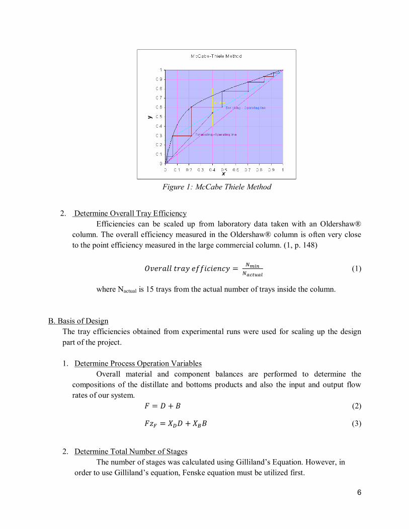
operating lines become the y=x line (1, p. 146). Figure 1 shows a graph on how

theoretical number of trays were determined using McCabe-Thiele Method

6

Figure 1: McCabe Thiele Method

2. Determine Overall Tray Efficiency

Efficiencies can be scaled up from laboratory data taken with an Oldershaw®

column. The overall efficiency measured in the Oldershaw® column is often very close

to the point efficiency measured in the large commercial column. (1, p. 148)

������������������� � ����������� (1)

where Nactual is 15 trays from the actual number of trays inside the column.

B. Basis of Design

The tray efficiencies obtained from experimental runs were used for scaling up the design

part of the project.

1. Determine Process Operation Variables

Overall material and component balances are performed to determine the

compositions of the distillate and bottoms products and also the input and output flow

rates of our system.

� � � � (2)

��� ��� � ��� (3)

2. Determine Total Number of Stages

The number of stages was calculated using Gilliland’s Equation. However, in

order to use Gilliland’s equation, Fenske equation must be utilized first.

7

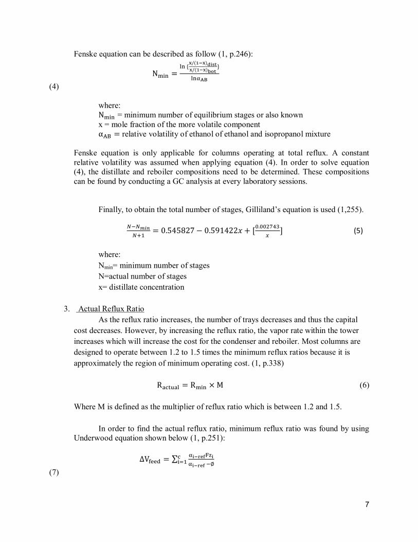
Fenske equation can be described as follow (1, p.246):

��������������������������������������������������������� !"# $#�%&'()*&+,-./&'()*&+01/ 2$#345

(4)

where: !"# = minimum number of equilibrium stages or also known

x = mole fraction of the more volatile component 678 relative volatility of ethanol of ethanol and isopropanol mixture

Fenske equation is only applicable for columns operating at total reflux. A constant

relative volatility was assumed when applying equation (4). In order to solve equation

(4), the distillate and reboiler compositions need to be determined. These compositions

can be found by conducting a GC analysis at every laboratory sessions.

Finally, to obtain the total number of stages, Gilliland’s equation is used (1,255).

��������������������������������������������9�����:; <=>?>@AB C <=>DE?AAF � GH=HHIJKLM N (5)

where:

Nmin= minimum number of stages

N=actual number of stages

x= distillate concentration

3. Actual Reflux Ratio

As the reflux ratio increases, the number of trays decreases and thus the capital

cost decreases. However, by increasing the reflux ratio, the vapor rate within the tower

increases which will increase the cost for the condenser and reboiler. Most columns are

designed to operate between 1.2 to 1.5 times the minimum reflux ratios because it is

approximately the region of minimum operating cost. (1, p.338)

OPQRSP$ O!"# TU (6)

Where M is defined as the multiplier of reflux ratio which is between 1.2 and 1.5.

In order to find the actual reflux ratio, minimum reflux ratio was found by using

Underwood equation shown below (1, p.251):

VWXYYZ [ 3-*\]^_`-3-*\]^�9aQ"b;

(7)

8

where:

VWXYYZ= change in vapor flow rate [lb/hour]

F = feed flow rate [kg/hour] 6 = relative volatility of compound i with respect to its c"= mass fraction in feed a = Underwood equation constant

The change in vapor flow rate in equation (7) can be solved using the formula expressed

in equation (7) (1, p.251).

VWXYYZ d(E C e+ (8)

where:

q= feed quality

By substituting equation (8) into equation (7), the constant a can be found. Based on

equation (7) and equation (8), it can be concluded that Underwood equation is a strong

function of feed quality. The constant a found in equation (7) is then substituted into

equation (9) to obtain the minimum vapor flow rate (1, p.251).

����������������W!"# [ 3-*\]^(fg-h,-./+3-*\]^�9aQ"b;

(9)

where:

D= distillate flow rate [kg/hour] i"hZ"jR = mass fraction of component i in distillate W!"#= minimum vapor flow rate [kg/hour]

Once W!"# is known, the minimum liquid flow rate, k!"# required is calculated from the

mass balance

����������������������������������������������������������k!"# W!"# C l (10)

where: k!"#= minimum liquid flow rate [kg/hour]

The internal reflux ratio solved using equation (9) and equation (10) can be converted to

external ratio as shown below:

mnfo!"# pn qr st-u;9pn qr st-u (11)

where:

9

mnqo!"#= minimum liquid to vapor ratio (internal reflux ratio)

mnfo!"#= minimum reflux ratio (external reflux ratio)

Once minimum external reflux ratio is found, the design engineer can then incorporate

the given range of 1.25 to 1.5 to calculate the actual reflux ratio required to achieve the

required separation.

4. Determine Actual Number of Trays

The actual numbers of trays are determined using the tray efficiency obtained

from the experiment. (1, p.148)

PQRSP$ v/w]1\]/-xyz{XX"Q"Y#Q| (12)

5. Determine the dimension of the column

Diameter of the tower is relatively insensitive to the changes in operating pressure

or temperature. The main determinant of the diameter is the vapor velocity. Fair’s method

is used to determine the diameter of the column. (1, p. 152)

��}���� �~ K��������������(��������+������(L�HH+ � (13)

Tower height can be determined using the number of trays in the column and the tray

spacing.

����� ������������ T ��}�������� (14)

6. Determine the Optimum Feed Location

An approximate estimate of the optimum feed-stage location, XYYZ can be

obtained using the Kirkbride equation.

�������������������������������� mv^]],9;v9v^]],o <=A�<���  8f m¡-.1¢\1¢yu1z¡]/wyu1z o £ ¤5h]/wyu1z¤¥h-.1¢\1¢yu1z¦I§ (15)

7. Reboiler and Condenser Duties

Energy balances are performed to determine the reboiler and condenser duties.

Condenser duty determines the amount of wash liquid flow in the tower to meet the

degree of rectification required for the lighter product. The reboiler in turn generates the

vapor flow in the tower to satisfy the degree of stripping required for the particular

separation and the quality of the heavy product.

¨��©���������� ���������� T ������������������ (16)

10

Apparatus:

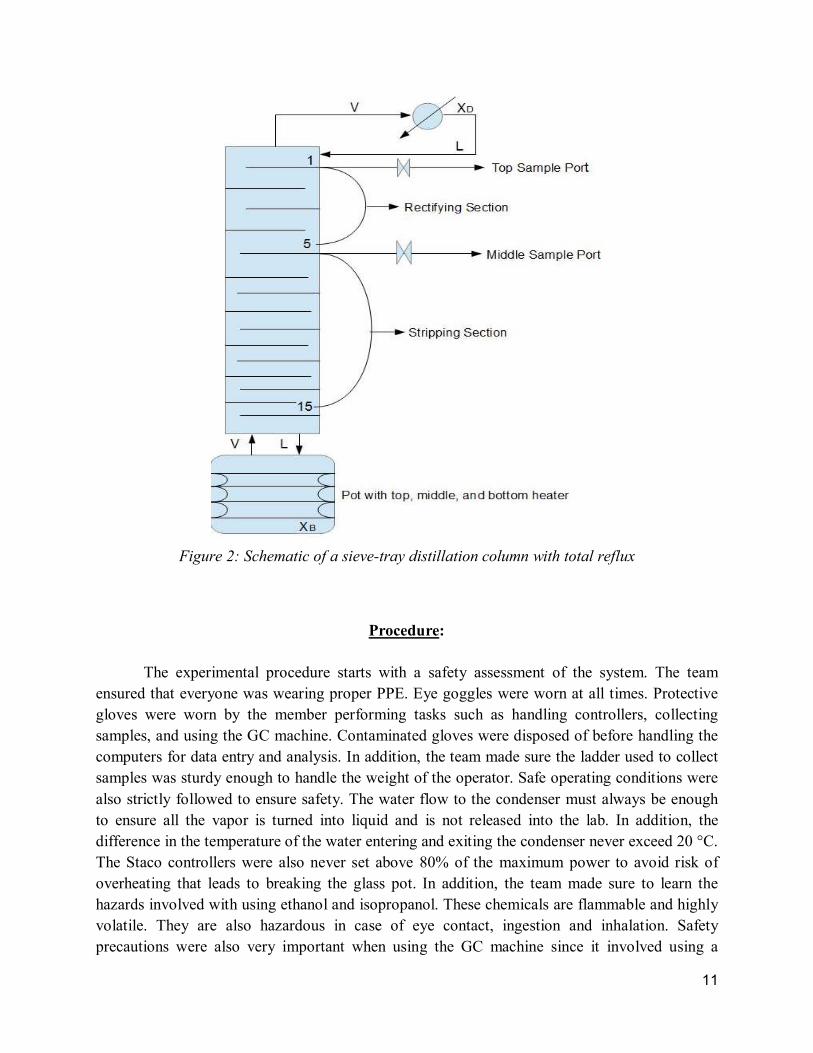
The experimental apparatus consists of a vacuum-jacketed 50 mm I.D. Oldershaw sieve-

tray distillation column operating at continuous total reflux. The column is split into two

sections. The first is a rectifying section containing the five top trays. The second a stripping

section containing the bottom ten trays. There are six thermocouples throughout the column that

measure the temperatures at different sections of the column and are shown on a monitor in

LabView. There is a still pot with three heaters in the bottom which contain the feed to this

system. Each heater has a separate Staco controller that determines how much energy is provided

to the still pot. At the top of the column, there is water-cooled condenser that condenses all the

vapor and sends it back down the column as liquid. There is a valve at the bottom of the column

that controls the flow of water into the condenser and a rotameter displaying a reading of the

water flow. Samples can be collected at two spots in the distillation column. The first is right

before the rectifying section (before the first stage) and the second is before the stripping section

(before the sixth stage). A Gas Chromatography (GC) machine is provided to analyze the

composition of the sample products. A schematic of the column is shown in Figure 2.

11

Figure 2: Schematic of a sieve-tray distillation column with total reflux

Procedure:

The experimental procedure starts with a safety assessment of the system. The team

ensured that everyone was wearing proper PPE. Eye goggles were worn at all times. Protective

gloves were worn by the member performing tasks such as handling controllers, collecting

samples, and using the GC machine. Contaminated gloves were disposed of before handling the

computers for data entry and analysis. In addition, the team made sure the ladder used to collect

samples was sturdy enough to handle the weight of the operator. Safe operating conditions were

also strictly followed to ensure safety. The water flow to the condenser must always be enough

to ensure all the vapor is turned into liquid and is not released into the lab. In addition, the

difference in the temperature of the water entering and exiting the condenser never exceed 20 °C.

The Staco controllers were also never set above 80% of the maximum power to avoid risk of

overheating that leads to breaking the glass pot. In addition, the team made sure to learn the

hazards involved with using ethanol and isopropanol. These chemicals are flammable and highly

volatile. They are also hazardous in case of eye contact, ingestion and inhalation. Safety

precautions were also very important when using the GC machine since it involved using a

12

syringe containing hazardous chemicals. Once a safety assessment of the system was complete,

the team was ready to operate the column.

The team started by setting the desired operating conditions for the column. This meant

using the Staco controllers to set the power provided to the heaters and using the control valve to

set the water flow rate into the condenser. Once these settings had been set, the team waited for

25-30 minutes to ensure the column is operating at a steady state condition. This was also

verified by observing the temperatures throughout the column and noting that there was no

fluctuation. Samples were collected from the two different ports for analysis once the column

had reached steady state. This was done by climbing the ladder and opening the valve for the

desired port and waiting for the liquid to run through a tube and into the collection vial. Once the

samples had been collected, the team ensured all sample valves had been closed. The team then

proceeded to change the operation conditions to the next desired state and repeated this

procedure.

For data analysis, the samples were run through a GC machine. To do this, 0.5 µL of the

sample was injected into the machine through a rubber septum using a syringe. The machine

produced a graph that allowed the team to determine the composition of the sample. For each

lab, the team started by analyzing the composition of the still pot since it’s the feed for the

column. The two samples collected from the two different ports at each operating condition were

also analyzed.

Design of Experiments:

In order to determine the efficiency of the column and how operating conditions affect it,

the column was run at many different settings. This design was chosen since it allowed the team

to study the effects of each controlled variable on the column efficiency. It also allowed the team

to determine whether the experimental data was reproducible or not. The design of experiments

is shown in Table 1.

Table 1: Design of experiments

Trial Experiment Outcome

1 Ran prepared samples through the GC

machine

Prepared a calibration curve for the GC

machine

2 Learned to operate the distillation

column

Experienced how different settings relate

to different operating parameters

13

3 Ran column at constant water flow and

different Staco settings

Learned how column efficiency relates to

the power settings

4 Ran column at higher constant water

flow and different Staco settings

Learned how column efficiency relates to

power settings and how controlled

variables interact

5 Ran column at constant Staco setting

and different water flows

Learned how column efficiency relates to

water flow

6 Repeated settings in previous labs Verified the reproducibility of obtained

data

7 Repeated settings in previous labs Repeated settings in previous labs

8 Ran column at different Staco and flow

rate settings

Obtain data for condenser design

Experimental Results:

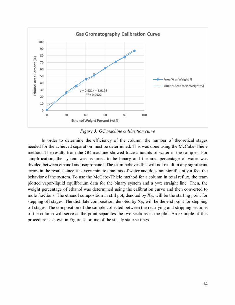
The GC machine provided information of the sample by showing a graph with a peak for

each component present in the sample. Each peak has an area percentage that is related to how

much of that particular component is present in the sample. Since the detector is not equally

sensitive to each of the components present in the sample, the team constructed a calibration

curve that relates the area percentage of ethanol to its weight percentage. This was done by

running prepared samples of known composition through the GC machine and plotting the

resulting area percentage against the known weight percentage. The resulting calibration curve is

shown in Figure 3.

14

Figure 3: GC machine calibration curve

In order to determine the efficiency of the column, the number of theoretical stages

needed for the achieved separation must be determined. This was done using the McCabe-Thiele

method. The results from the GC machine showed trace amounts of water in the samples. For

simplification, the system was assumed to be binary and the area percentage of water was

divided between ethanol and isopropanol. The team believes this will not result in any significant

errors in the results since it is very minute amounts of water and does not significantly affect the

behavior of the system. To use the McCabe-Thiele method for a column in total reflux, the team

plotted vapor-liquid equilibrium data for the binary system and a y=x straight line. Then, the

weight percentage of ethanol was determined using the calibration curve and then converted to

mole fractions. The ethanol composition in still pot, denoted by XB, will be the starting point for

stepping off stages. The distillate composition, denoted by XD, will be the end point for stepping

off stages. The composition of the sample collected between the rectifying and stripping sections

of the column will serve as the point separates the two sections in the plot. An example of this

procedure is shown in Figure 4 for one of the steady state settings.

y = 0.921x + 5.9198

R² = 0.9922

0

10

20

30

40

50

60

70

80

90

100

0 20 40 60 80 100

Eth

an

ol A

rea

Pe

rce

nt

(%)

Ethanol Weight Percent (wt%)

Gas Gromatography Calibration Curve

Area % vs Weight %

Linear (Area % vs Weight %)

15

Figure 4: McCabe-Thiele diagram for Staco setting = 60% and water flow = 0.053kg/s

The efficiency of the column is determined using Equation 1. The efficiency was

determined for the different steady state settings for changes in the two controlled variables. The

efficiency of this type of column is then used in the design procedure. The results are presented

graphically in Figures 5,6, and 7.

16

Figure 5: Efficiency at 0.053 kg/s water flow and changing Staco setting

Figure 6: Efficiency at 0.041 kg/s water flow and changing Staco setting

0

0.1

0.2

0.3

0.4

0.5

0.6

0.7

0.8

40 45 50 55 60 65 70 75

Eff

icie

ncy

Staco Setting (%)

Efficiency Vs Staco Setting @ 0.053kg/s Water

Flow

Stripping Section

Rectifying Section

Total Column

0

0.1

0.2

0.3

0.4

0.5

0.6

0.7

0.8

30 35 40 45 50 55 60 65 70 75

Eff

icie

ncy

Staco Setting (%)

Efficiency Vs Staco Setting @ 0.041kg/s Water

Flow Rate

Stripping Section

Rectifying Section

Total Column

17

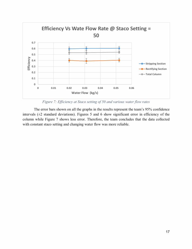
Figure 7: Efficiency at Staco setting of 50 and various water flow rates

The error bars shown on all the graphs in the results represent the team’s 95% confidence

intervals (±2 standard deviations). Figures 5 and 6 show significant error in efficiency of the

column while Figure 7 shows less error. Therefore, the team concludes that the data collected

with constant staco setting and changing water flow was more reliable.

0

0.1

0.2

0.3

0.4

0.5

0.6

0.7

0 0.01 0.02 0.03 0.04 0.05 0.06

Eff

icie

ncy

Water Flow (kg/s)

Efficiency Vs Wate Flow Rate @ Staco Setting =

50

Stripping Section

Rectifying Section

Total Column

18

Discussion:

The experimental results shown in Figures 5, 6 and 7 show that the maximum efficiency

obtained from the column is 53.3%. Figures 5 and 6 show the effect of changing the power

supplied to the heaters in the still pot. Figure 5 shows us that even though the efficiencies of the

two sections were changing with the change in power, the overall efficiency of the column

remained constant. Figure 6 shows constant efficiencies throughout the column but a decrease at

the highest point of power supplied. The results shown in Figure 6 were obtained at a lower

condenser water flow rate than that in Figure 5. Therefore, the team believes there wasn’t enough

water flow in the condenser to turn all the vapor to liquid. Which lead to lower concentrations of

ethanol in the samples, thus lowering efficiency. Figure 7 shows the effect of changing the

condenser water flow rate on the efficiency. According to the graph, there is no change in

efficiency at the different water flow settings. The team believes this is because as long as the

condenser is able to turn all the vapor going up the column into liquid, the efficiency will not

change. Even though the water flow rates were set to very low settings, the power provided to

the heaters was quite low too. Meaning there wasn’t a large amount of vapor going up the

column and even low water flow rates were enough to condense all the vapor.

Some constraints on the results obtained were because the team had to follow the limiting

operating conditions on the distillation column. Otherwise, it would have been worthwhile to try

higher Staco settings to see if the trend in Figure 6 were to continue. In addition, the results could

have been improved if the team had tried varying the water flow rate at constant Staco setting

that is higher than 50%. These two extra sets of experiments would allow the team to determine

if their hypothesis on the water flow rate’s effect on the system is accurate or not. Also, more

repeat data could have been

19

Design Calculations:

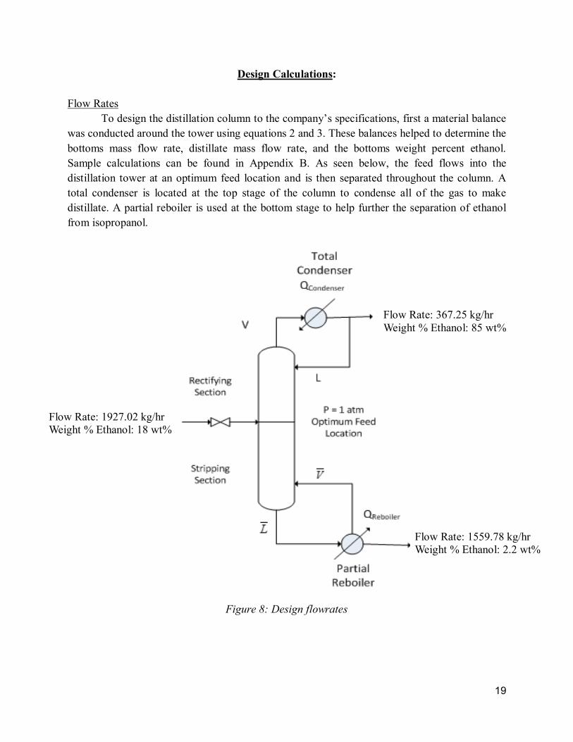
Flow Rates

To design the distillation column to the company’s specifications, first a material balance

was conducted around the tower using equations 2 and 3. These balances helped to determine the

bottoms mass flow rate, distillate mass flow rate, and the bottoms weight percent ethanol.

Sample calculations can be found in Appendix B. As seen below, the feed flows into the

distillation tower at an optimum feed location and is then separated throughout the column. A

total condenser is located at the top stage of the column to condense all of the gas to make

distillate. A partial reboiler is used at the bottom stage to help further the separation of ethanol

from isopropanol.

Figure __: Flow rates around design column

Figure 8: Design flowrates

Flow Rate: 1927.02 kg/hr

Weight % Ethanol: 18 wt%

Flow Rate: 367.25 kg/hr

Weight % Ethanol: 85 wt%

Flow Rate: 1559.78 kg/hr

Weight % Ethanol: 2.2 wt%

20

Total Number of Stages

After material balances were conducted on the tower to obtain the flow rates and weight-

percent’s, the number of stages was then calculated using Gilliland’s Equation 5 (4, p. 253).

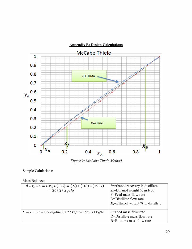
McCabe-Thiele was not used in the design of the column because of how close the VLE curve

and the x=y line ran to each other, as seen in Figure 10 in Appendix B. Accurate “steps” could

not have been analyzed, so a different approach was taken. No method is perfect for modeling

non-ideal systems, but all sources indicated that using the following approach was one of the

simplest ways to achieve a design. In order to use Gilliland’s equation, Fenske and Underwood

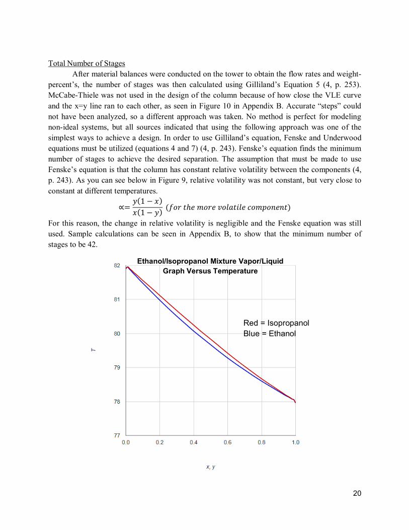
equations must be utilized (equations 4 and 7) (4, p. 243). Fenske’s equation finds the minimum

number of stages to achieve the desired separation. The assumption that must be made to use

Fenske’s equation is that the column has constant relative volatility between the components (4,

p. 243). As you can see below in Figure 9, relative volatility was not constant, but very close to

constant at different temperatures.

� �(E C F+F(E C �+�(�������}��������������}������+ For this reason, the change in relative volatility is negligible and the Fenske equation was still

used. Sample calculations can be seen in Appendix B, to show that the minimum number of

stages to be 42.

Ethanol/Isopropanol Mixture Vapor/Liquid

Graph Versus Temperature

Red = Isopropanol

Blue = Ethanol

21

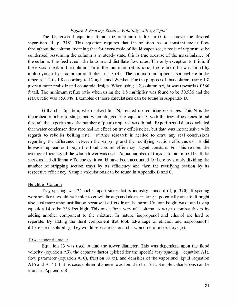
Figure 9. Proving Relative Volatility with x,y,T plot

The Underwood equation found the minimum reflux ratio to achieve the desired

separation (4, p. 248). This equation requires that the solution has a constant molar flow

throughout the column, meaning that for every mole of liquid vaporized, a mole of vapor must be

condensed. Assuming the column is at steady state, this is true because of the mass balance of

the column. The feed equals the bottom and distillate flow rates. The only exception to this is if

there was a leak in the column. From the minimum reflux ratio, the reflux ratio was found by

multiplying it by a common multiplier of 1.8 (3). The common multiplier is somewhere in the

range of 1.2 to 1.8 according to Douglas and Wankat. For the purpose of this column, using 1.8

gives a more realistic and economic design. When using 1.2, column height was upwards of 360

ft tall. The minimum reflux ratio when using the 1.8 multiplier was found to be 30.936 and the

reflux ratio was 55.6848. Examples of these calculations can be found in Appendix B.

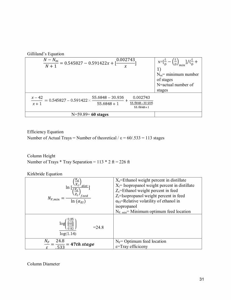
Gilliand’s Equation, when solved for “N,” ended up requiring 60 stages. This N is the

theoretical number of stages and when plugged into equation 5, with the tray efficiencies found

through the experiments, the number of plates required was found. Experimental data concluded

that water condenser flow rate had no effect on tray efficiencies, but data was inconclusive with

regards to reboiler boiling rate. Further research is needed to draw any real conclusions

regarding the difference between the stripping and the rectifying section efficiencies. It did

however appear as though the total column efficiency stayed constant. For this reason, the

average efficiency of the whole tower was used. Actual number of trays is found to be 113. If the

sections had different efficiencies, it could have been accounted for here by simply dividing the

number of stripping section trays by its efficiency and then the rectifying section by its

respective efficiency. Sample calculations can be found in Appendix B and C.

Height of Column

Tray spacing was 24 inches apart since that is industry standard (4, p. 370). If spacing

were smaller it would be harder to crawl through and clean, making it potentially unsafe. It might

also cost more upon instillation because it differs from the norm. Column height was found using

equation 14 to be 226 feet high. This made for a very tall column. A way to combat this is by

adding another component to the mixture. In nature, isopropanol and ethanol are hard to

separate. By adding the third component that took advantage of ethanol and isopropanol’s

difference in solubility, they would separate faster and it would require less trays (5).

Tower inner diameter

Equation 13 was used to find the tower diameter. This was dependent upon the flood

velocity (equation A9), the capacity factor (picked for the specific tray spacing – equation A1),

flow parameter (equation A10), fraction (0.75), and densities of the vapor and liquid (equation

A16 and A17 ). In this case, column diameter was found to be 12 ft. Sample calculations can be

found in Appendix B.

22

Feed stage

Feed stage was found using the Kirkbride equation (equation 15). The assumptions

surrounding this equation were the same as specified in the other models used (3). Example

calculations can be found in the Appendix B. The optimum feed stage found was 47 when

corrected for tray efficiency. Trays 1-46 made up the rectifying section, while trays 58-113 made

up the stripping section.

Temperature of Feed

Temperature of the feed should be at bubble point to allow for separation to start as soon

as the feed enters the distillation tower (4, p. 198). This temperature needed to be in between the

two boiling points. The boiling point of ethanol is 78.37 degrees C and the boiling point of

isopropanol is 82.6 degrees C. The temperature of the feed should be 81.84 degrees C because it

is relative to the weight percent’s (weighted average).

Temperature of Condenser water

For cost purposes, cooling water can simply be at room temperature – around 21 C. It is

sufficient because room temperature water is still far below the boiling points of either

substance.

Temperature of Reboiler

Because of how hot the reboiler must be, special care must be taken to insulate the

outside of the apparatus and there should be a barrier between the operator and the reboiler.

Operators should make sure to wear heat shirts when interacting with the reboiler. Regardless of

the power set in the experiments, temperature of the pot never went above 82 degrees C. For this

reason, the temperature of the reboiler should be set to 82 degrees C.

Amount of Steam Utilized

An energy balance could be conducted around the column to provide the operators with

the amount of steam to let into the column to power it. Condensor duties could show how much

energy was taken out of the column, while reboiler duties would show how much energy was put

into the system. This is something that should be done before installation, or could be adjusted

during start up to help fine tune optimum separation.

23

Final Design:

Table 2: Experimental Design

Number of Stages 120 Eq. 5

Tray Spacing 24 inches Literature (Wankat, p. 370)

Height of Column 240 ft Eq. 14

Tower Inner Diameter 12 ft Eq. 13

Optimum Feed Stage Stage 50 Eq. 15

Outlet Stage of Ethanol Stage 1 Practical Design

Outlet Stage of Isopropanol Stage 120 Practical Design

Type of Column Sieve Tray Given by company

Table 3: Operating Parameters

Flow Rate: Distillate 367 kg/hr Eq. 2 & 3

Flow Rate: Bottoms 1560 kg/hr Eq. 2 & 3

Flow Rate: Feed 1927 kg/hr Given maximum

Feed Temperature 81.8 degrees C Boiling point relative average

Condensor Temperature 21 degrees C Most economical

Reboiler Temperature 82 degrees C Experimental

This design should provide the most economic and safe operating conditions.

24

Conclusions & Recommendations:

This work has led to the following conclusions and recommendations.

1. Experimental data concludes that water condenser flow rate has no effect on tray

efficiencies, but data is inconclusive with regards to reboiler boiling rate. For this reason

it is recommended that boiling rate (how hard solution is boiling) of the reboiler is kept as

constant as possible until further research is done regarding its effects on separation. It

appears as though total column efficiency stays constant while the stripping section and

rectifying section efficiencies change, but as mentioned earlier, more research is needed.

2. 1.8 was the chosen multiplier of the minimum reflux ratio because it was recommended

in literature. This being said, other multipliers were recommended in other sources. In

general 1.2 to 1.8 seemed to be the most commonly found range. This could be a source

of error for this column, but is recommended for use because it makes the column much

more reasonable and economically sized than when using a smaller multiplier.

3. An energy balance should be taken around the column to decide how much steam needs

to be used to power the column. Reboiler and condenser duties can be utilized as to

account for how much energy is being put into the system and how much is being taken

out. This needs to be done before start up to get a basis setting, but can be adjusted.

Further research needs to be done to find out how much adjusting the steam pressure will

affect separation.

4. It is recommended that another component be added to the mixture to make for an easier

separation. This could save money because the column would not have to be quite as

high.

25

Notations:

English

mnfo!"# = minimum reflux ratio (external reflux ratio)

mnqo!"# = minimum liquid to vapor ratio (internal reflux ratio) i7 = Liquid mole fraction of species A (ethanol) i"hZ"jR = Mass fraction of component i in distillate ��ª��« = Flooding velocity

B (mole/s) = Molar bottom flow rate

Cp,et (J/g.C) = Specific heat capacity of ethanol

Cp,iso (J/g.C) = Specific heat capacity of isopropanol

D (mole/s) = Molar distillate flow rate

F (mole/s) = Molar feed flow rate

I.D. (ft) = Inside diameter

L (mol/s) = Molar flow rate of liquid going back into the column

mF (g/s) = Feed mass flow rate

mvap (g/s) = Mass flow rate of vapor in distillate

MW (g/gmol) = Molar weight of vapor

mw (g/s) = Mass flow rate of water

MWet (g/mol) = Molecular mass of ethanol

MWiso (g/mol) = Molecular mass of isopropanol

N = Area available for vapor flow

Nactual = Number of stage based on actual reflux ratio

Nmin = Minimum number of stage or number of stage at total reflux

QC (J/s) = Heat in condenser

QR (J/s) = Heat in reboiler

R = Reflux ratio TB ( C) = Temperature of bottom

TD ( C) = Temperature of distillate

TF ( C) = Temperature of feed

uvap (m/s) = Mass flow rate of vapor in distillate

V (mol/s) = Molar flow rate of vapor

X = Mole fraction of the more volatile component

xB = Mass fractions of ethanol in bottom

XB,et = Ethanol weight fraction at bottom

XB,iso = Isopropanol weight fraction at bottom

XD,et = Ethanol weight fraction at distillate

26

XD,iso = Isopropanol weight fraction at distillate

XF,et = Ethanol mass fraction at feed

XF,iso = Isopropanol mass fraction at feed

Greek

a = Underwood equation constant

αEI =Relative volatility of ethanol in isopropanol

ΔHB (J/mol) = Enthalpy of bottom

ΔHD (J/mol) = Enthalpy of distillate

ΔHF (J/mol) = Enthalpies of feed

ΔHvap,et (J/mol) = Enthalpy of vaporization of ethanol

ΔHvap,iso (J/mol) = Enthalpy of vaporization of isopropanol

ΔHvap,mix (J/mol) = Enthalpy of vaporization of et-iso mixture

ε =Tray efficiency ¬ =Fraction of the column across cross sectional area that is available for

vapor flow above the tray

ρet (g/m3) = Density of ethanol

ρiso (g/m3) = Density of isopropanol ­ = surface tension

27

References:

1. Wankat, P., Separation Process Engineering Includes Mass Transfer Analysis, Pearson

Education, New York, 2012.

2. U.S. Energy Information Administration - EIA - Independent Statistics and Analysis

(Vacuum distillation is a key part of the petroleum refining process).

http://www.eia.gov/todayinenergy/detail.cfm?id=9130. Accessed 10-18-2014.

3. Douglas, J. M. (1988). Conceptual Design of Chemical Processes. McGraw-Hill Book

Company.

4. Wankat, Phillip. Separation Process Enginering. International ed. Prentice Hall. 110-140,

301-340. Print.

5. Thacker, Quinn. Lab 5: Seperation of Mixture. Web.

http://www.chemistryland.com/CHM130FieldLab/Lab5/Lab5.html. Accessed 11-1-2013

28

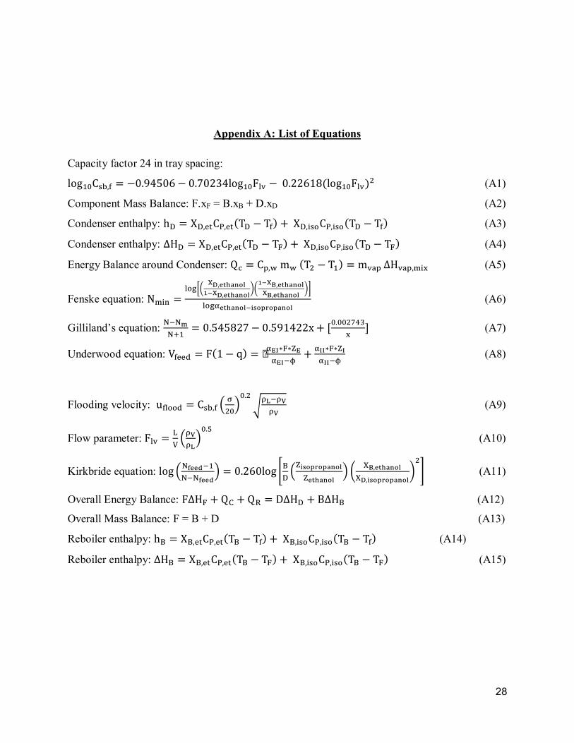
Appendix A: List of Equations

Capacity factor 24 in tray spacing:

���;H®j¯hX C<=D?><� C <=B<A°?���;Hd$± C �<=AA�E@(���;Hd$±+I (A1)

Component Mass Balance: F.xF = B.xB + D.xD (A2)

Condenser enthalpy: ²f ³fhYR®´hYR(µf C µX+ ��³fh"j¶®´h"j¶(µf C µX+ (A3)

Condenser enthalpy: ·¸f ³fhYR®´hYR(µf C µ_+ ��³fh"j¶®´h"j¶(µf C µ_+ (A4)

Energy Balance around Condenser: ¹Q ®ºh»�¼»�(µI C µ;+ ¼±Pº�V¸±Pºh!"g (A5)

Fenske equation: !"# $¶½¾£ ¿¥h]/wyu1z)*¿¥h]/wyu1z¦£)*¿5h]/wyu1z¿5h]/wyu1z ¦À$¶½3]/wyu1z*-.1¢\1¢yu1z (A6)

Gilliland’s equation: v9vtv:; <=>?>@AB C <=>DE?AAi � GH=HHIJKLg N (A7)

Underwood equation: WXYYZ d(E C e+ 3ÂÃÄ_Ä¡Â3ÂÃ9Å � 3ÃÃÄ_Ä¡Ã3ÃÃ9Å (A8)

Flooding velocity: ÆX$¶¶Z ®j¯hX m ÇIHoH=I~ÈÉ9ÈÊÈÊ (A9)

Flow parameter: d$± nq mÈÊÈÉoH=Ë (A10)

Kirkbride equation: ��� mv^]],9;v9v^]],o <=A�<���  8f m¡-.1¢\1¢yu1z¡]/wyu1z o £ ¤5h]/wyu1z¤¥h-.1¢\1¢yu1z¦I§ (A11)

Overall Energy Balance: dV¸_ � ¹Ì � ¹Í lV¸f � ÎV¸8 (A12)

Overall Mass Balance: F = B + D (A13)

Reboiler enthalpy: ²8 ³8hYR®´hYR(µ8 C µX+ ��³8h"j¶®´h"j¶(µ8 C µX+ (A14)

Reboiler enthalpy: ·¸8 ³8hYR®´hYR(µ8 C µ_+ ��³8h"j¶®´h"j¶(µ8 C µ_+ (A15)

29

Appendix B: Design Calculations

Figure 9: McCabe-Thiele Method

Sample Calulations:

Mass Balances

� Ä �Ï Ä � �FÏÐ �(= @>+ (= D+ Ä (= E@+ Ä (EDAB+ °�B=AB�Ñ�'�� β=ethanol recovery in distillate

Ze=Ethanol weight % in feed

F=Feed mass flow rate

D=Distillate flow rate

Xe=Ethanol weight % in distillate

� � � � = 1927kg/hr-367.27 kg/hr= 1559.73 kg/hr

F=Feed mass flow rate

D=Distillate mass flow rate

B=Bottoms mass flow rate

30

�� ��� � ��� =

1927*.18=.85*367.27+F�*1559.73; F�=.022

Fenske Equation

ÓÔ�� �Õ £� �((E C �+(E C �++¦�Õ(Ö+

β = fractional recovery of light key in the

distillate

δ = fractional recovery of heavy key in the

bottoms

α = relative volatility

=

42.1975

Underwood Equation

×�ÏÏ« �(E C Ø+ � ÖÙÚ Ä � Ä ÒÙÖÙÚ C Û � ÖÚÚ Ä � Ä ÒÚÖÚÚ CÛ q=feed quality

αEI= relative volatility of

ethanol in isopropanol

αII= relative volatility of

isopropanol in isopropanol

φ=

=1.11

×Ô�� � ÖÙÚ Ä � Ä FÙÖÙÚ CÛ � ÖÚÚ Ä � Ä FÚÖÚÚ CÛ

Vmin=Minimum vapor flow

from reboiler to column

D=Mass flow rate of distillate

=11353.6 kg/hr

(Ü�+Ô�� (EE°>°=��Ñ�'��� +Ô�� °<=D°�� (Ý�+Ô�� Minimum reflux ratio

£Ü�¦ (Ü�+Ô�� Ä E=@ >>=�@?@ mÝ�o= Reflux Ratio

31

Gilliland’s Equation Ó C ÓÔÓ � E <=>?>@AB C <=>DE?AAF � G<=<<AB?°F N

x=[� C m�o��N'(� �E+

Nm= minimum number

of stages

N=actual number of

stages

N=59.89= 60 stages

Efficiency Equation

Number of Actual Trays = Number of theoretical / ε = 60/.533 = 113 stages

Column Height

Number of Trays * Tray Separation = 113 * 2 ft = 226 ft

Kirkbride Equation

�h�� ��G m

FÏF�o«�Þ�m�Ï��o�ÏÏ«N�

�Õ�(ÖÙÚ+

Xe=Ethanol weight percent in distillate

Xi= Isopropanol weight percent in distillate

Ze=Ethanol weight percent in feed

Zi=Isopropanol weight percent in feed

αEI=Relative volatility of ethanol in

isopropanol

NF, min= Minimum optimum feed location

=24.8

Ó�ß A?=@= >°° àáâã�äâåæç NF= Optimum feed location

ε=Tray efficiceny

Column Diameter

32

� è ?×éêëì�íë(������+��ª��«(°�<<+ V= Feed mass flow rate ��ª��«=flood velocity íë ����� density éêë= molecular weight vapor

n= area available for vapor flow

�̈���=capacity factor

ρ’s = densities of liquid and vapor î= surface tension

��ª��« �̈���( îA<+H=IHèíÝ C íëíë

��ª��« <=>°>E(A=AB>A< +H=IHè?D=>> C <=E<<E<=E<<E B=B

���;H Þ̈ïh� C<=D?><��C <=B<A°?���;H�ªëC <=AA�E@(���;H�ªë+I

���;H Þ̈ïh� C<=D?><� C <=B<A°?���;H(<=<B@+ C<=AA�E@(���;H(<=<B@++I = =0.5351

�ð ��ªë Ü× èíëíÝ

Ü×èíëíÝ (EE°>°=�?>C °�B+EE°>°=�?>Ä è= E<<E?D=>> <=<B@

Suggested (Wankat p. 370) fraction is 0.75

íë �éêëñ� ����íÝ �éêÝñ�

� ~ K(;òIË+ÄI=IÄKJ=JK�(=óË+(J=J+(=JË+ (H=;HH;+ (L�HH+ = 12.0697 ft

33

Appendix C: Calibration Calculations

34

Appendix D: Intermediate Design Table

Table 4: Design Parameters

Aspect Justification

Height of Column (m) Design Equation

Inner Diameter (m) Design Equation

Feed Stage Design Equation

Outlet Stage - Ethanol Design Equation

Outlet Stage – Isopropanol Design Equation

Number of Stages - Stripping Experimentally

Number of Stages - Rectifying Experimentally

Type of column Sieve Tray Column

Table 5: Operating Parameters

Aspect Justification

Temperatures Experimentally

Water Condenser Rate (}L'�+ Experimentally

Feed Rate (}L'�+ Given

Auxiliary Steam (Pa) Calculated