design of an adaptive backstepping controller for 2 dof...
TRANSCRIPT
1
DESIGN OF AN ADAPTIVE BACKSTEPPING CONTROLLER FOR 2 DOF PARALLEL ROBOT
By
JING ZOU
A THESIS PRESENTED TO THE GRADUATE SCHOOL
OF THE UNIVERSITY OF FLORIDA IN PARTIAL FULFILLMENT OF THE REQUIREMENTS FOR THE DEGREE OF
MASTER OF SCIENCE
UNIVERSITY OF FLORIDA
2014
2
© 2014 Jing Zou
3
ACKNOWLEDGMENTS
The author expresses his deep gratitude to his advisor, Dr. John K. Schueller, for
guiding him throughout his work, and for his support and dedication. The author also
expresses his sincere appreciation to his committee Dr. Carl Crane III for his guidance
and help. The author also extends his thanks to Dr. Warren Dixon for his support.
4
TABLE OF CONTENTS page
ACKNOWLEDGMENTS .................................................................................................. 3
LIST OF TABLES ............................................................................................................ 5
LIST OF FIGURES .......................................................................................................... 6
ABSTRACT ..................................................................................................................... 9
CHAPTER
1 INTRODUCTION .................................................................................................... 11
1.1 Background ....................................................................................................... 11 1.2 Related Work .................................................................................................... 12
2 ADAPTIVE BACKSTEPPING CONTROLLER FOR PARALLEL ROBOTS ............ 14
2.1 Kinematics and Dynamics Analysis for Parallel Robots .................................... 14 2.1.1 Kinematics Analysis ................................................................................. 14
2.1.2 Dynamics Analysis .................................................................................. 24 2.2 Adaptive Backstepping Controller for Parallel Robots....................................... 26
2.2.1 Lyapunov Based Design of the Controller ............................................... 26 2.2.2 Verification on the Implementation of the Controller ................................ 30
3 ANALYSIS FOR THE 2 DOF PARALLEL ROBOT ................................................. 32
3.1 Kinematic and Singularity Analysis of the 2 DOF Parallel Robot ...................... 32 3.2 Accuracy and Efficiency Analysis for the 2 DOF Parallel Robot ....................... 36
3.3 Modeling for the 2 DOF Parallel Robot ............................................................. 44 3.3.1 Dynamics Model for the 2 DOF Parallel Robot ........................................ 44
3.3.2 Verification of the dynamics model .......................................................... 51 3.4 Dynamics Model for the 2 DOF Parallel Robot with Dnamics and Kinematics
Uncertainties ........................................................................................................ 59
4 CONTROL SYSTEM DESIGN FOR 2 DOF PARALLEL ROBOT ........................... 68
4.1 Adaptive Backstepping Controller for the 2 DOF Parallel Robot Model with Uncertainties ........................................................................................................ 68
4.2 Simulation Result and Discussion ..................................................................... 74
5 CONCLUSION AND FUTURE WORK .................................................................... 90
REFERENCES .............................................................................................................. 91
BIOGRAPHICAL SKETCH ............................................................................................ 93
5
LIST OF TABLES
Table: page 3-1 Partial derivative distribution of qa1 to x (rad/dm) ............................................... 42
3-2 Partial derivative distribution of qa2 to x (rad/dm) ............................................... 42
3-3 Partial derivative distribution of qa1 to y (rad/dm) ............................................... 43
3-4 Partial derivative distribution of qa2 to y (rad/dm) ............................................... 43
6
LIST OF FIGURES
Figure: page 3-1 Symmetrical 2 DOF parallel robot ....................................................................... 32
3-2 The coordinate system of the 2 DOF parallel robot ............................................ 33
3-3 Area definition 1 .................................................................................................. 35
3-4 Area definition 2 .................................................................................................. 35
3-5 Restricted zone for C .......................................................................................... 36
3-6 Partial derivative of qa1 to x ............................................................................... 40
3-7 Partial derivative of qa1 to y ............................................................................... 41
3-8 Partial derivative of qa2 to x ............................................................................... 41
3-9 Partial derivative of qa2 to y ............................................................................... 42
3-10 Robot arm coordinate system ............................................................................. 44
3-11 Revised robot coordinate system ....................................................................... 45
3-12 Force analysis for bar BC and DC ...................................................................... 48
3-13 Force analysis for bar AB and ED ...................................................................... 49
3-14 SimMechanics model for the 2 DOF parallel robot ............................................. 52
3-15 Value of qa1 in mathmetic model and SimMechanics modle ............................. 53
3-16 Value of qa2 in mathematical model and SimMechanics model ......................... 54
3-17 Angular velocity of qa1 in mathematical model and SimMechanics model ......... 54
3-18 Angular velocity of qa2 in mathematical model and SimMechanics model ......... 55
3-19 Input torque at A in mathematical model and SimMechanics model .................. 55
3-20 Input torque at E in mathematical model and SimMechanics model .................. 56
3-21 Error between two models for qa1 ...................................................................... 56
3-22 Error between two models for qa2 ...................................................................... 57
3-23 Error between two models in angular velocity of qa1 ......................................... 57
7
3-24 Error between two models in angular velocity of qa2 ......................................... 58
3-25 Error between two models for input torque at A.................................................. 58
3-26 Error between two models for input torque at E.................................................. 59
3-27 2 DOF parallel robot with dynamics and kinematics uncertainties ...................... 60
3-28 Force analysis for bar BC and DC ...................................................................... 61
3-29 Force analysis for bar AB and ED ...................................................................... 62
4-1 Simulation Block for Control System .................................................................. 75
4-2 Destination point and tracking trajectory (ABE) .................................................. 76
4-3 Error in x direction for set point tracking (ABE) ................................................... 77
4-4 Error in y direction for set point tracking (ABE) ................................................... 77
4-5 Destination point and tracking trajectory (BE)..................................................... 78
4-6 Error in x direction for set point tracking (BE) ..................................................... 78
4-7 Error in y direction for set point tracking (BE) ..................................................... 79
4-8 Destination point and tracking trajectory (ABU) .................................................. 79
4-9 Error in x direction for set point tracking (ABU)................................................... 80
4-10 Error in y direction for set point tracking (ABU)................................................... 80
4-11 Destination point and tracking trajectory (BU) .................................................... 81
4-12 Error in x direction for set point tracking (BU) ..................................................... 81
4-13 Error in y direction for set point tracking (BU) ..................................................... 82
4-14 Desired trajectory and tracking trajectory (ABE) ................................................. 83
4-15 Error in x direction for trajectory tracking (ABE).................................................. 84
4-16 Error in y direction for trajectory tracking (ABE).................................................. 85
4-17 Desired trajectory and tracking trajectory (BE) ................................................... 85
4-18 Error in x direction for trajectory tracking (BE) .................................................... 86
4-19 Error in y direction for trajectory tracking (BE) .................................................... 86
8
4-20 Desired trajectory and tracking trajectory (ABU)................................................. 87
4-21 Error in x direction for trajectory tracking (ABU) ................................................. 87
4-22 Error in y direction for trajectory tracking (ABU) ................................................. 88
4-23 Desired trajectory and tracking trajectory (BU) ................................................... 88
4-24 Error in x direction for trajectory tracking (BU) .................................................... 89
4-25 Error in y direction for trajectory tracking (BU) .................................................... 89
9
Abstract of Thesis Presented to the Graduate School of the University of Florida in Partial Fulfillment of the Requirements for the Degree of Master of Science
DESIGN OF AN ADAPTIVE BACKSTEPPING CONTROLLER FOR 2 DOF PARALLEL
ROBOT
By
Jing Zou
May 2014
Chair: John K. Schueller Major: Mechanical Engineering
It is very common in robot tracking control that controllers are designed based on
the exact kinematic model of the robot manipulator. However, because of measurement
errors and changes of states, the original kinematic model is no longer accurate and will
degrade the control result. Besides, the structure of the controllers are always much
more complicated for robots with the targets expressed in task space, due to the
transformation from joint space to task space. In this thesis, a controller is designed for
parallel robot systems with kinematics and dynamics uncertainties through
backstepping control and adaptive control. Backstepping control is used to simplify the
structure of the controller whose target is expressed in the task space and manage the
transformation between the errors in task space and joint space. Adaptive control is
utilized to compensate for uncertainties in both dynamics and kinematics.
A realization of the proposed controller is achieved based on the Two Degree of
Freedom (2 DOF) parallel robot designed in this thesis. The simulation of the control
system is carried out using SimMechanics™ in MATLAB®. Compared to the simulation
result of the system controlled by the backstepping controller, simulation results of the
control system indicate that the proposed controller has robust performance with regard

10
to dynamics and kinematics uncertainties. The proposed controller gives desired
performance to achieve the research goal.
11
CHAPTER 1 INTRODUCTION
1.1 Background
Robot manipulators have been widely used in our current society, especially in
manufacturing industries. They make their appearance in almost every automatic
assembly line. The efficiency and accuracy of the robot manipulators has a great
influence on the production and quality of the product. Large number of robot
manipulators have been designed over the last half century, and several of these have
become standard platforms for R&D efforts [1]. A robot manipulator is a movable chain
of links interconnected by joints. One end is fixed to the ground, and a hand or end
effector that can move freely in space is attached at the other end [2].
Serial robot manipulator, designed as series of links connected by motor-
actuated joints that extend from a base to an end-effector, are the most common
industrial robots. However, parallel robot manipulator, a mechanical system that uses
several computer-controlled serial chains to support a single platform or end-effector,
have the following potential advantages over serial manipulators: better accuracy,
higher stiffness and payload capability, higher velocity, lower moving inertia, and so on.
The goal of this thesis is to come up with a new nonlinear control strategy that
can enhance robustness of the robot manipulator to both kinematics and dynamics
uncertainties through explore the kinematic and dynamics characteristics of the parallel
robots.
12
1.2 Related Work
This work is focused on the kinematics and dynamics analysis of the parallel
robot manipulators and the design of a controller to achieve robust performance with
regard to kinematics uncertainties, dynamics certainties.
Robot manipulators are highly nonlinear in their dynamics and kinematics. And
even more nonlinearities appear in parallel robot manipulators. In order to have a good
tracking performance of parallel robot manipulators, people try to compensate for the
nonlinearities and use feedback PD control to minimize the tracking error. In [3] and [4],
a nonlinear PD controller was proposed by using the nonlinear terms in robot dynamics
as nonlinear feedback to cancel those terms and PD feedback to control the tracking
error. This controller is very sensitive to uncertainties in the robot model as it needs very
accurate knowledge of the robot dynamics to cancel the nonlinear terms in the system.
To make the controller robust to the dynamic uncertainties of the parallel robot
manipulator, adaptive control, high gain control and high frequency control methods are
introduced. In [5] and [6], an adaptive controller was created with an estimator for the
dynamic parameters of the robot to compensate for the uncertainties. And in [7], sliding
mode control method is applied to decentralize uncertain dynamic parameters of the
robot manipulator to get a more robust performance. Those controllers work well with
parallel robots having uncertainties in dynamics. However, since there are no estimators
to predict the uncertain parameters in kinematic functions and the decentralization
method is not applied to uncertain terms appearing in the kinematics, they are not
robust to kinematic uncertainties. In [8] and [9], adaptive controllers are proposed to
make the whole system resistant to uncertainties in both dynamics and kinematics
through design of estimator to predict and compensate the uncertain terms in both
13
dynamic and kinematic functions. The controllers give good control results. The
researchers produce integrated controllers to compensate for both dynamics and
kinematics uncertainties. As the kinematics uncertainties are decoupled from the control
input, much more mathematical analysis and structure complexity is required for the
controllers. A robust backstepping controller is proposed in [10]. The design needs less
effort, but its Lyapunov analysis is based on the slow-varying assumption on some
parameters, which means the robot is not influenced by potentially arbitrarily large and
fast external torques, and this is a bad assumption for parallel robot manipulators,
where arbitrarily large and fast external torques can appear due to geometric
constraints on the bars of the robot. And in [11], a controller is proposed for system with
uncertainties in dynamics, kinematics and actuator, desired armature current model of
the actuator is necessary to finish the Lyapunov analysis and controller design for the
system.
In this thesis, the mathematical analysis of the Jacobian matrix of a parallel robot
helps to conclude that it is linear in physical parameters. And then through the
implementation of backstepping control and adaptive control, a controller which is
robust to uncertainties in dynamics and kinematics is constructed. With the application
of backstepping control, massive mathematical analysis according to the decoupling of
control input and kinematics uncertainties is avoided. And the adaptive control has a
good performance for the parallel robot with arbitrarily large and fast dynamics caused
by geometric constraints.
14
CHAPTER 2 ADAPTIVE BACKSTEPPING CONTROLLER FOR PARALLEL ROBOTS
2.1 Kinematics and Dynamics Analysis for Parallel Robots
2.1.1 Kinematics Analysis
Here a kinematic structure that has a rigid base connected to a rigid end effector
by means of n serial kinematic chains in parallel is discussed. Each set of serial
kinematic chain is defined as a “leg”. The th “leg” has degrees of freedom,
, collected in a vector . Let be the total number of joints:
∑ , and be the vector of all joint angles: (
) . The rest of
analysis in this section is written with reference to [12].
Not all joints of the parallel structure can be actuated independently; the end
effector of the structure has, at each instant in time, a number of degrees of freedom,
, which can never be larger than six. This means that of the joints can be
actuated independently (these are called the driving joints), and that their motion
completely determines the motion of all other joints (these joints are the driven
joints). The relationships between the driving and the driven joints are determined by
the so-called closure equations.
Velocity closure:
Given position closure, the velocity of all joints in each leg must be such that the
end point of that leg moves with the same spatial velocity as its connection point at the
end effector. Mathematically, velocity closure is represented, for example, by the
following set of linear equations:
15
[
] [
] (2-1)
with the Jacobian matrix of the th leg.
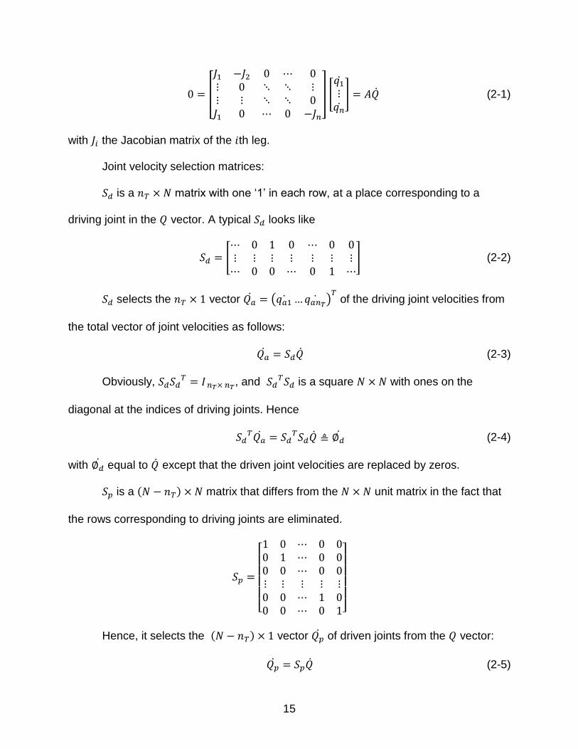
Joint velocity selection matrices:
is a matrix with one ‘1’ in each row, at a place corresponding to a
driving joint in the vector. A typical looks like
[
] (2-2)
selects the vector ( )
of the driving joint velocities from
the total vector of joint velocities as follows:
(2-3)
Obviously,
, and is a square with ones on the
diagonal at the indices of driving joints. Hence
(2-4)
with equal to except that the driven joint velocities are replaced by zeros.
is a ( ) matrix that differs from the unit matrix in the fact that
the rows corresponding to driving joints are eliminated.
[ ]
Hence, it selects the ( ) vector of driven joints from the vector:
(2-5)
16
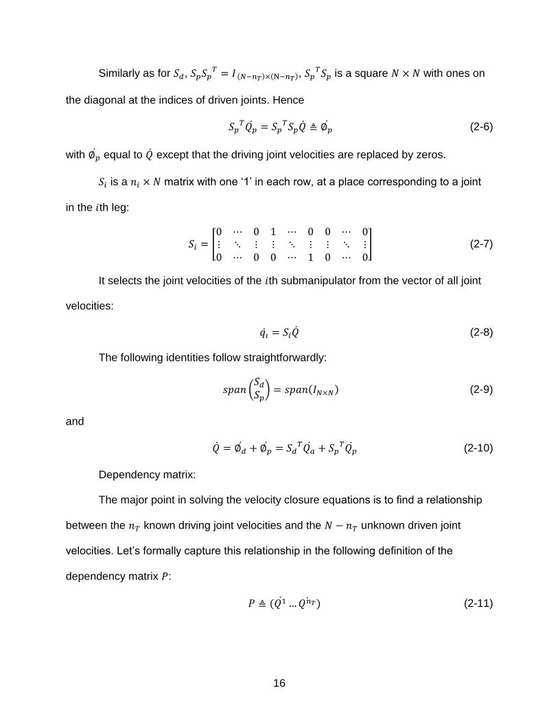
Similarly as for , ( ) ( ),
is a square with ones on
the diagonal at the indices of driven joints. Hence
(2-6)
with equal to except that the driving joint velocities are replaced by zeros.
is a matrix with one ‘1’ in each row, at a place corresponding to a joint
in the th leg:
[
] (2-7)
It selects the joint velocities of the th submanipulator from the vector of all joint
velocities:
(2-8)
The following identities follow straightforwardly:
(
) ( ) (2-9)
and
(2-10)
Dependency matrix:
The major point in solving the velocity closure equations is to find a relationship
between the known driving joint velocities and the unknown driven joint
velocities. Let’s formally capture this relationship in the following definition of the
dependency matrix :
( ) (2-11)
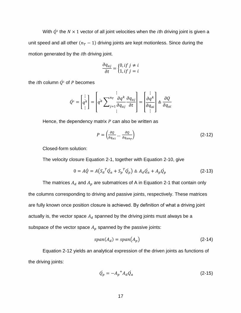
17
With the vector of all joint velocities when the th driving joint is given a
unit speed and all other ( ) driving joints are kept motionless. Since during the
motion generated by the th driving joint.
{
the th column of becomes
[
] [
∑
] [
]
Hence, the dependency matrix can also be written as
(
) (2-12)
Closed-form solution:
The velocity closure Equation 2-1, together with Equation 2-10, give
(
) (2-13)
The matrices and are submatrices of A in Equation 2-1 that contain only
the columns corresponding to driving and passive joints, respectively. These matrices
are fully known once position closure is achieved. By definition of what a driving joint
actually is, the vector space spanned by the driving joints must always be a
subspace of the vector space spanned by the passive joints:
( ) ( ) (2-14)
Equation 2-12 yields an analytical expression of the driven joints as functions of
the driving joints:
(2-15)
18
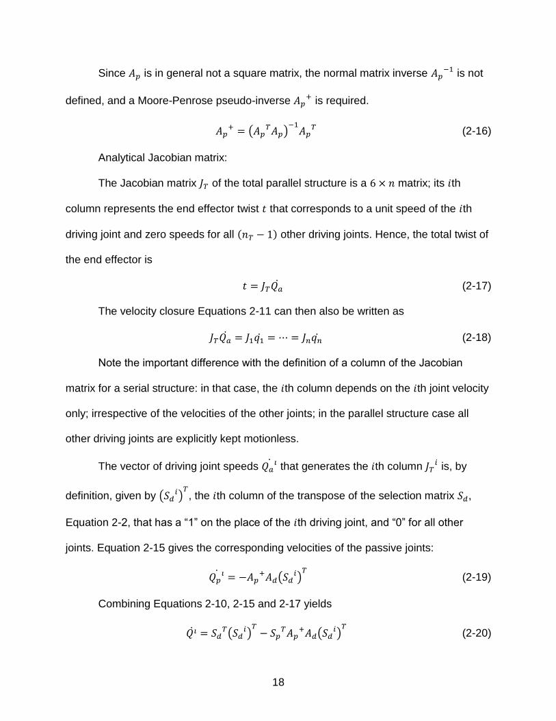
Since is in general not a square matrix, the normal matrix inverse is not
defined, and a Moore-Penrose pseudo-inverse is required.
(
)
(2-16)
Analytical Jacobian matrix:
The Jacobian matrix of the total parallel structure is a matrix; its th
column represents the end effector twist that corresponds to a unit speed of the th
driving joint and zero speeds for all ( ) other driving joints. Hence, the total twist of
the end effector is
(2-17)
The velocity closure Equations 2-11 can then also be written as
(2-18)
Note the important difference with the definition of a column of the Jacobian
matrix for a serial structure: in that case, the th column depends on the th joint velocity
only; irrespective of the velocities of the other joints; in the parallel structure case all
other driving joints are explicitly kept motionless.
The vector of driving joint speeds that generates the th column
is, by
definition, given by ( )
, the th column of the transpose of the selection matrix ,
Equation 2-2, that has a “1” on the place of the th driving joint, and “0” for all other
joints. Equation 2-15 gives the corresponding velocities of the passive joints:
( )
(2-19)
Combining Equations 2-10, 2-15 and 2-17 yields
(
)
( )
(2-20)

19
This equation gives the th column of the dependency matrix in of Equation 2-
11. Using Equations 2-8 and 2-18, the th column of is then found as
(2-21)
The right-hand sides of these equations first select the joint velocities of one of
the serial subchains from the vector of all joint velocities, and multiplies these subchain
joint velocities with the subchain Jacobian matrix to obtain the corresponding end
effector twist. All serial subchains are equivalent to calculate a column of the Jacobiann
since they all have to follow the same twist of the end effector. Repeating the above-
mentioned procedure for all driving joints gives, for all ,
( ) (2-22)
with the dependency matrix as defined in (11).
Jacobian matrix property analysis:
According to Equation 2-20, Equation 2-22 can be transformed into
( )
(( )
(
) )
(( )
(
) )
(2-23)
where is a matrix. Usually with proper arrangement of in and ,
.
Then it can be derived that
(2-24)
The conclusion that , , , , , and are all linear in physical
parameters is obtained from their previous descriptions in this section.
20
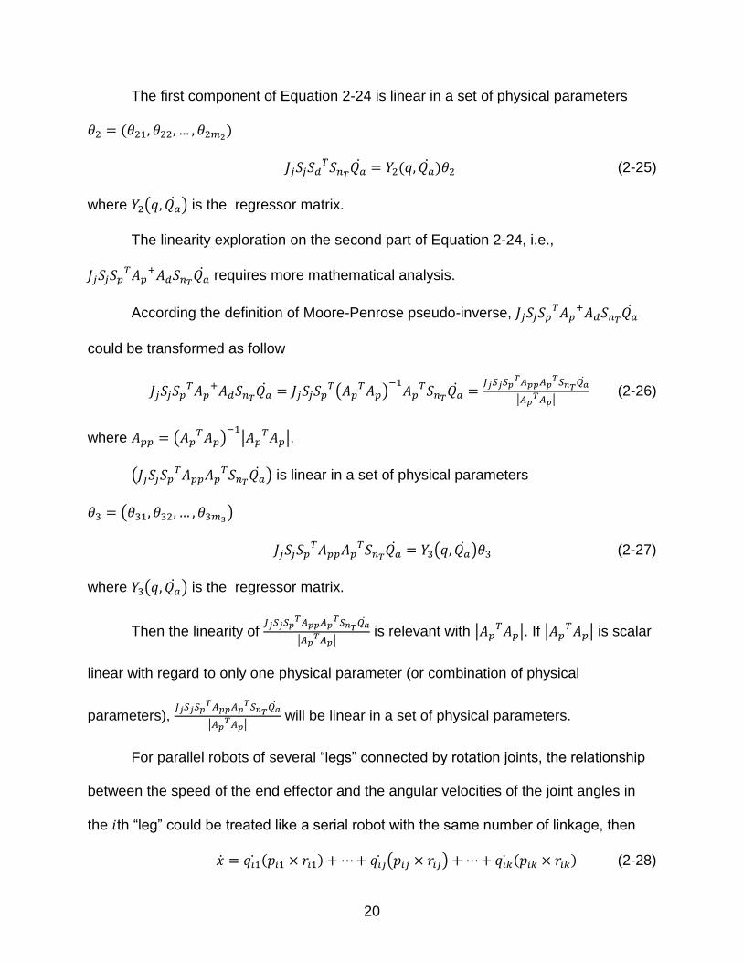
The first component of Equation 2-24 is linear in a set of physical parameters
( )
( ) (2-25)
where ( ) is the regressor matrix.
The linearity exploration on the second part of Equation 2-24, i.e.,
requires more mathematical analysis.
According the definition of Moore-Penrose pseudo-inverse,
could be transformed as follow
( )
| |
(2-26)
where ( )
|
|.
(
) is linear in a set of physical parameters
( )
( ) (2-27)
where ( ) is the regressor matrix.
Then the linearity of
| |
is relevant with | |. If |
| is scalar
linear with regard to only one physical parameter (or combination of physical
parameters),
| |
will be linear in a set of physical parameters.
For parallel robots of several “legs” connected by rotation joints, the relationship
between the speed of the end effector and the angular velocities of the joint angles in
the th “leg” could be treated like a serial robot with the same number of linkage, then
( ) ( ) ( ) (2-28)

21
where is the direction vector of angular velocity for th rotation joint, i.e. , and is
the position vector from th joint to ( )th joint. Given , with the direction
vector of and the length of , and is a ( ) vector function of
measurable variables and the azimuth angles of joint axis. This leads to
( )( )
(2-29)
then
[
]
where corresponds to the length of a bar starting from a passive (driven) joint in the
th leg, ,
, are the first, second and third element of vector function
. is
the number of passive joint in one leg and assume all “legs” have the same number of
passive joints. Then, denotes the number of all the passive joints.
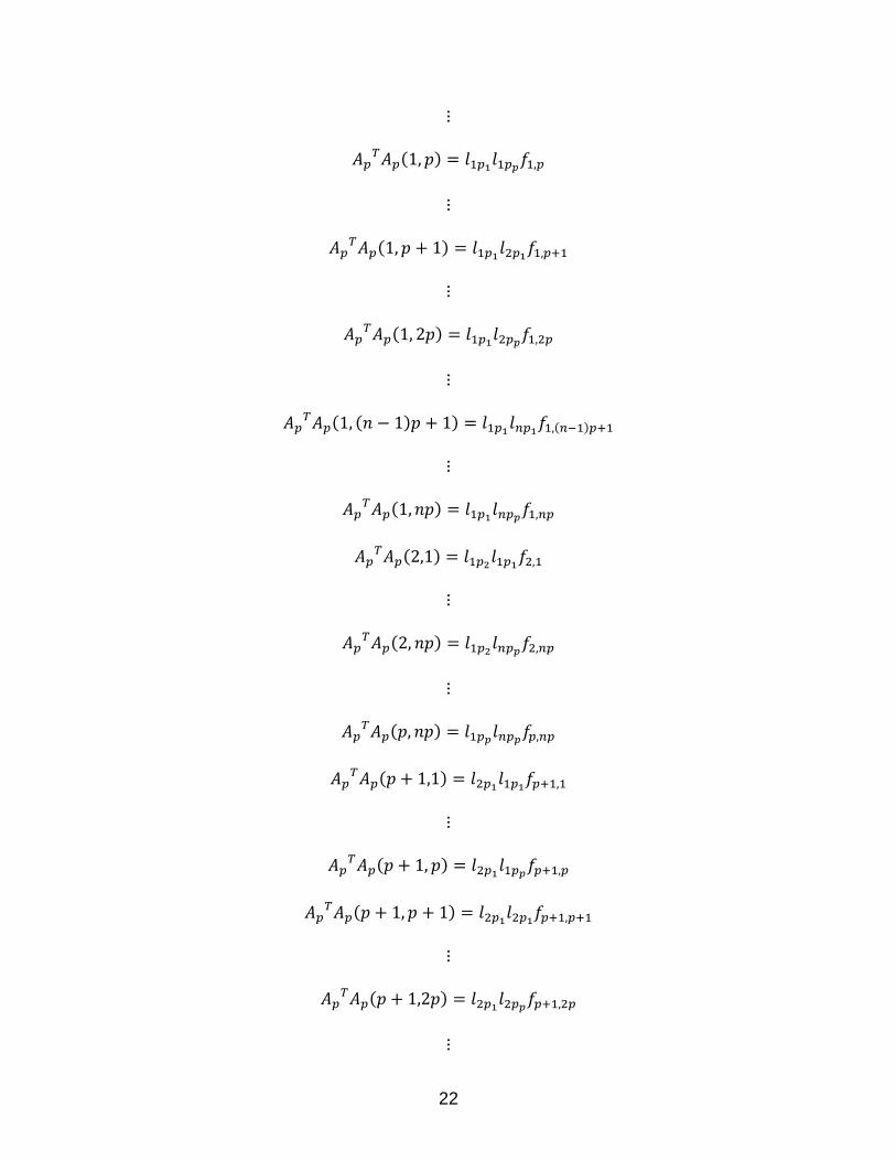
To get the properties of | |, firstly
needs to be calculated. The
calculation process and results of is shown below.
The component of matrix in row 1, column 1 is
( ) (
)
The same goes for other components of
( )
22
( )
( )
( )
( ( ) )
( )
( )
( )
( )
( )
( )
( )
( )
( )
23
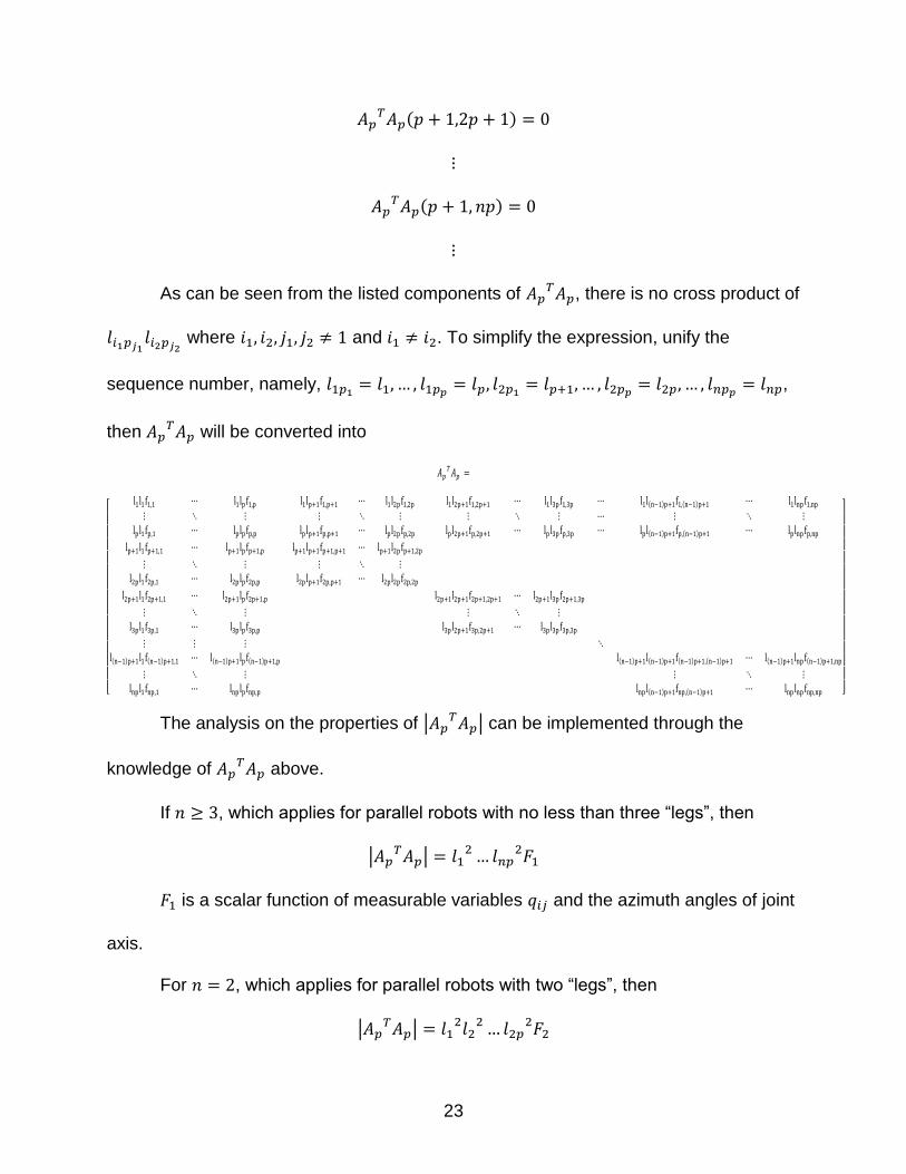
( )
( )
As can be seen from the listed components of , there is no cross product of
where and . To simplify the expression, unify the
sequence number, namely,
,
then will be converted into
[
( ) ( )
( ) ( )
( ) ( ) ( ) ( ) ( ) ( ) ( ) ( ) ( ) ( )
( ) ( ) ]
The analysis on the properties of | | can be implemented through the
knowledge of above.
If , which applies for parallel robots with no less than three “legs”, then
| |
is a scalar function of measurable variables and the azimuth angles of joint
axis.
For , which applies for parallel robots with two “legs”, then
| |

24
is also a scalar function of measurable variables and the azimuth angles of
joint axis.
Therefore, | | is linear in a combination of physical parameters
( ), and
| |
is also linear in a combination of physical parameters
. Thus
| | ( )
| |
( ) (2-30)
Bring Equation 2-29 back to Equation 2-26
| |
( ) ( ) ( ) (2-31)
where ( ) is the regressor matrix and is the combination of physical parameters
in and .
The second part of Equation 2-24, i.e.,
is linear in a set of
physical parameters ( )
Substitutes Equations 2-31 and 2-26 into Equation 2-24 yields
( ) ( ) ( ) (2-32)
where ( ) is the regressor matrix and is the combination of physical parameters
in and .
Hence, the kinematics functions (or the kinematic model) of the proposed parallel
robot is linear in a set of physical parameters ( ).
2.1.2 Dynamics Analysis
The dynamic model of a parallel robot with uncertain parameters is:
( ) ( ) ( ) (2-33)
25
where and are the angular acceleration and angular velocity of the active joints,
( ) is the inertia matrix, ( ) is a vector function containing Coriolis
and centrifugal forces, ( ) is a vector function consisting of gravitational forces.
There are several properties for the dynamic equation:
Property 1: The inertia matrix ( ) is symmetric and uniformly positive–definite
for all .
Property 2: The matrix (
( ) ( )) is skew-symmetric so that
(
( ) ( )) for all .
Property 3: The dynamic model as described by (10) is linear in a set of physical
parameters ( ) as
( ) ( ) ( ) ( )
where ( ) is called the dynamic regressor matrix.
Therefore, for the parallel robot connected by rotational joints and with same
number of linkage in each “leg”, both their kinematic and dynamic models are linear in
sets of physical parameters or sets of combination of physical parameters. Since all
uncertain parameters in both dynamics and kinematics are those physical parameters,
they can be separated and arranged into uncertain parameters vectors. Uncertain
parameters in dynamics are collected in vector and uncertain parameters in
kinematics are collected in vector . Adaptive control can then be applied to estimate
those uncertainties and compensate for them. And the designed controller would have
robust performance with regard to uncertain dynamics and kinematics.
26
2.2 Adaptive Backstepping Controller for Parallel Robots
This section is focused on designing a controller that gives asymptotical tracking
result in task-space for the proposed parallel robot. Meanwhile, the controller is robust
to kinematic and dynamics uncertainties.
2.2.1 Lyapunov Based Design of the Controller
Let , , denote the tracking error of the end-effector, the position of the end-
effector and the destination position of the end-effector. And for simplicity, replace
( ) with . Then
(2-34)
Taking the time derivative on both sides of Equation 2-34 and substituting
Equation 2-32 into it
(2-35)
here backstepping control is introduced through plus and subtract and on the
left side of Equation 2-35. is the estimate Jacobian matrix of the parallel robot, where
all uncertain elements of in the Jacobian matrix are replaced by corresponding
elements in , which are the estimators of those uncertain elements in . .
is a value which can be designed to achieve specified goals. And Equation 2-35 is
transformed into
(2-36)
27
where is the error between the set of physical parameters and the
estimator of the same set of physical parameters ; , and take the
derivative of result in .
Now can be designed as
( )
(2-37)
Substitute and into the dynamics function of the parallel
robot, i.e., Equation 2-33
( ) ( ) ( ) ( )( ) ( )( ) ( )
( ) ( ) ( ) ( ) ( ) (2-38)
Applying Property 3 in Equation 2-38
( ) ( ) ( ) (2-39)
Equation 2-39 can be reformulated as
( ) ( ) ( ) (2-40)
Defining the error between the set of physical parameters and the
estimator of the same set of physical parameters . Select the Lyapunov candidate as
( )
(2-41)
The derivative of the Lyapunov candidate is
( )
( )
(2-42)
Substitute Equaitons 2-37 and 2-39 into Equation 2-42 and apply Property 2
( ) ( ( ) ( ) )
( )
28
( ( ) ) (
( ) ( ) )
( ( ) )
(2-43)
Design the input controller as
( ) (2-44)
Substitute Equation 2-44 into Equation 2-43
( ( ) ( ) )
( ( ) )
( )
( )
(2-45)
For simplicity, replace ( ) with . Now we propose the adaptation
laws for and as follows
(2-46)
(2-47)
where and are designed positive numbers.
Substitute Equations 2-46, 2-47 into Equation 2-45
(2-48)
where is a negative semi-definite function.

29
Barbalate’s Lemma Corollary: If a scalar function ( ), is such that
( ) is lower bounded by zero
( ) ( )
( ) and ( ) is uniformly continuous in time
Then ( ) , as .
It has already been proven that is a negative semi-definite function along the
trajectories of ( ) and is a positive definite function, which mean is
decreasing and the value of is always bigger than 0. Therefore, could be lower
bounded by . Moreover
{
⇒ (2-49)
Under the reasonable assumption that ( ) , it can be drawn from Equation
2-49 that
( ) ( ) ∫ (
( )
)
⇒
{
{
(2-50)
Equation 2-48 could then be rewritten as
( ( ))
where √ . Take the derivative of and substitute Equation 2-16 into the
derivative
√ √ ( )
According to the results in Equation 2-50

30
√ ( ) ⇒
⇒ √
Consequently, 1) is lower bounded by ; 2) ; and 3)
√ and is uniformly continuous. All the conditions in Barbalate’s Lemma
Corollary are satisfied. Applying Barbalate’s Lemma Corollary to the Lyapunov
candidate in Equation 2-42 leads to the conclusion √ , as , i.e.,
, as .
The designed controller could achieve asymptotical tracking for the proposed
parallel robot.
2.2.2 Verification on the Implementation of the Controller
is a given desired value and . and are the sets of some constant
uncertain physical parameters and would never expand to infinity, thus, .
Singularities in kinematics and dynamics could be avoided by the selection of working
area, which guarantees , . Apply the conclusions from Equation 2-29
to Equations 2-25 and 2-26, , ,
( ),
and gives the following results
{
⇒
{
⇒
Introduce the above results in the equation

31
Thence, all those designed and measured values have been proven to be
bounded.
could be measured and are made of measurable parameters, from
Equaiton 2-26, is achievable. Through integration of , is obtained. The value of
can be acquired from the equation . is a given desired value and
known, can be calculated through
( ) and is calculated by taking
the derivative of . is measurable, then is available from . Using
Equation 2-25, the value of is accessible, and take integration of gives .
Consequently, all elements of the control input can be constructed.
All designed and measured values are bounded and the control input is
implementable. Therefore, the controller is implementable.
32
CHAPTER 3 ANALYSIS FOR THE 2 DOF PARALLEL ROBOT
3.1 Kinematic and Singularity Analysis of the 2 DOF Parallel Robot
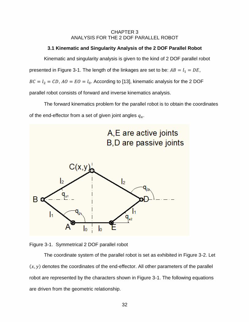
Kinematic and singularity analysis is given to the kind of 2 DOF parallel robot
presented in Figure 3-1. The length of the linkages are set to be: ,
, . According to [13], kinematic analysis for the 2 DOF
parallel robot consists of forward and inverse kinematics analysis.
The forward kinematics problem for the parallel robot is to obtain the coordinates
of the end-effector from a set of given joint angles .
Figure 3-1. Symmetrical 2 DOF parallel robot
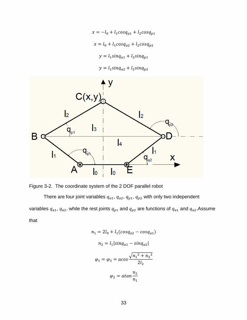
The coordinate system of the parallel robot is set as exhibited in Figure 3-2. Let
( ) denotes the coordinates of the end-effector. All other parameters of the parallel
robot are represented by the characters shown in Figure 3-1. The following equations
are driven from the geometric relationship.
33
Figure 3-2. The coordinate system of the 2 DOF parallel robot
There are four joint variables , , , with only two independent
variables , . while the rest joints and are functions of and .Assume
that
( )
| |
√
34
Two solutions exist for the forward kinematics.
Solution 1 (up-configuration):
Solution 2 (down-configuration):
Inverse kinematics:
The inverse kinematics problem for the parallel robot is to obtain a set of joint
angles from given coordinates of the end-effector. Assume that
(
(( ) )
√( ) ) (3-1)
(
(( ) )
√( ) ) (3-2)
(
) (3-3)
(
) (3-4)
then,
(3-5)
(3-6)
And those are the solutions for the inverse kinematic analysis.
Singularity:
Due to the analysis in [13], singularity happens under three cases.
35
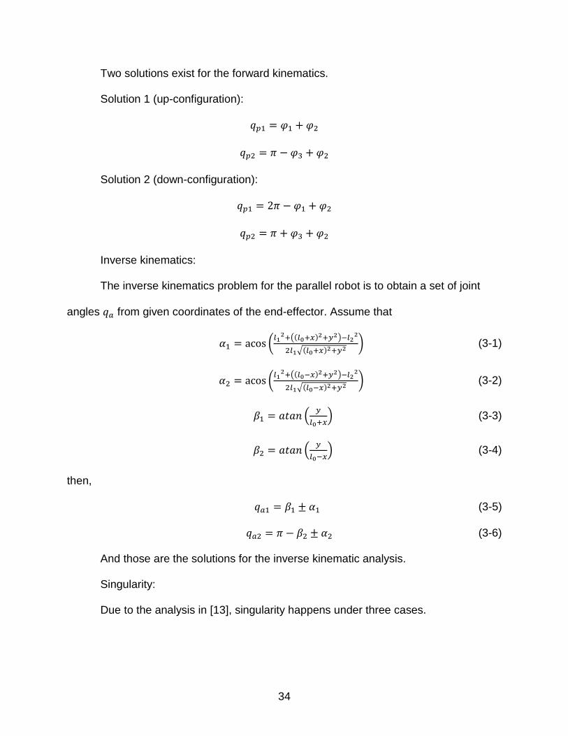
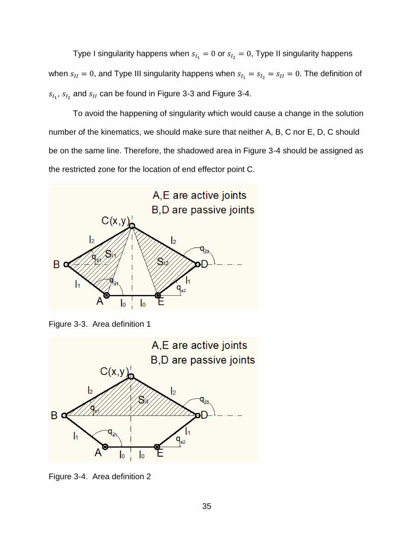
Type I singularity happens when or , Type II singularity happens
when , and Type III singularity happens when . The definition of
, and can be found in Figure 3-3 and Figure 3-4.
To avoid the happening of singularity which would cause a change in the solution
number of the kinematics, we should make sure that neither A, B, C nor E, D, C should
be on the same line. Therefore, the shadowed area in Figure 3-4 should be assigned as
the restricted zone for the location of end effector point C.
Figure 3-3. Area definition 1
Figure 3-4. Area definition 2
36
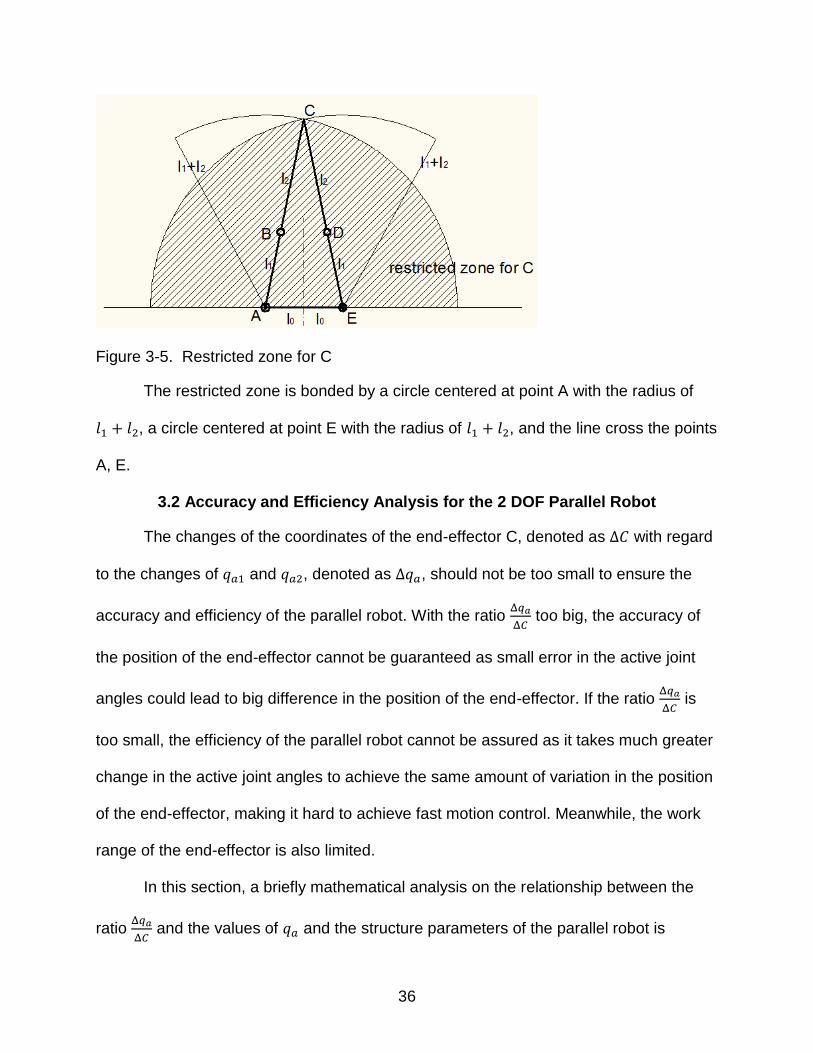
Figure 3-5. Restricted zone for C
The restricted zone is bonded by a circle centered at point A with the radius of
, a circle centered at point E with the radius of , and the line cross the points
A, E.
3.2 Accuracy and Efficiency Analysis for the 2 DOF Parallel Robot
The changes of the coordinates of the end-effector C, denoted as with regard
to the changes of and , denoted as , should not be too small to ensure the
accuracy and efficiency of the parallel robot. With the ratio
too big, the accuracy of
the position of the end-effector cannot be guaranteed as small error in the active joint
angles could lead to big difference in the position of the end-effector. If the ratio
is
too small, the efficiency of the parallel robot cannot be assured as it takes much greater
change in the active joint angles to achieve the same amount of variation in the position
of the end-effector, making it hard to achieve fast motion control. Meanwhile, the work
range of the end-effector is also limited.
In this section, a briefly mathematical analysis on the relationship between the
ratio
and the values of and the structure parameters of the parallel robot is

37
performed. This could forge a general understanding about their interactions and
support with some guidelines on the selections of those according to the specific
requirements.
First, the derivatives of and with regard to x and y value of the end-
effector are calculated.
Recall the inverse kinematic analysis result in section 3.1. By choosing the
mechanical structure, Equations 3-5 and 3-6 can be narrowed to
(3-7)
(3-8)
Assume that
(( ) )
√( )
(( ) )
√( )
Take the partial derivatives of and with regard to and
( )(( )
)
(( ) )
( )(( )
)
(( ) )
(( )
)
(( ) )
(( )
)
(( ) )
38
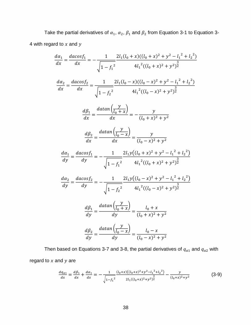
Take the partial derivatives of , , and from Equation 3-1 to Equation 3-
4 with regard to and
√
( )(( )
)
(( ) )
√
( )(( )
)
(( ) )
(
)
( )
(
)
( )
√
(( )
)
(( ) )
√
(( )
)
(( ) )
(
)
( )
(
)
( )
Then based on Equations 3-7 and 3-8, the partial derivatives of and with
regard to and are
√
( )(( )
)
(( ) )
( ) (3-9)
39
√
( )(( )
)
(( ) )
( ) (3-10)
√
(( )
)
(( ) )
( ) (3-11)
√
(( )
)
(( ) )
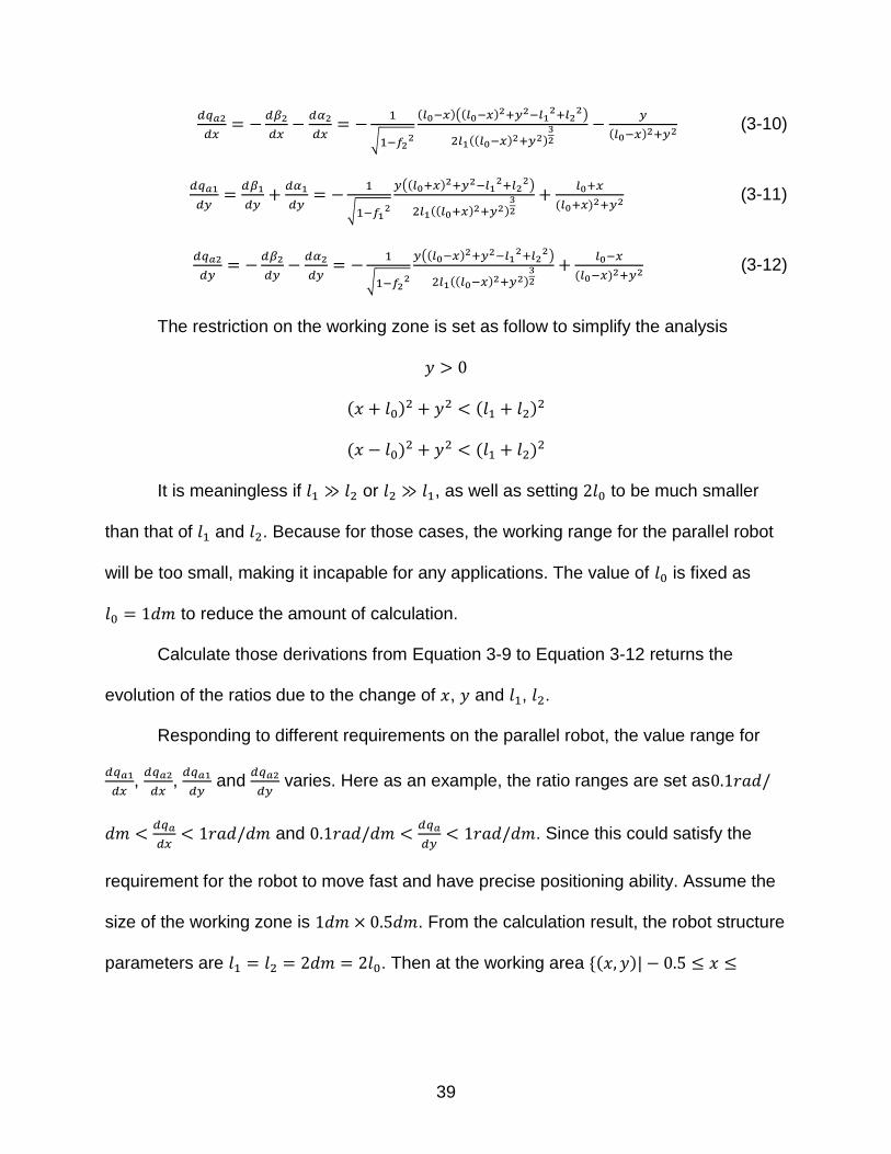
( ) (3-12)
The restriction on the working zone is set as follow to simplify the analysis
( ) ( )
( ) ( )
It is meaningless if or , as well as setting to be much smaller
than that of and . Because for those cases, the working range for the parallel robot
will be too small, making it incapable for any applications. The value of is fixed as
to reduce the amount of calculation.
Calculate those derivations from Equation 3-9 to Equation 3-12 returns the
evolution of the ratios due to the change of , and , .
Responding to different requirements on the parallel robot, the value range for
,
,
and
varies. Here as an example, the ratio ranges are set as
and
. Since this could satisfy the
requirement for the robot to move fast and have precise positioning ability. Assume the
size of the working zone is . From the calculation result, the robot structure
parameters are . Then at the working area ( )|
40
, the ratio range requirements are met. The corresponding angle
range is: , .
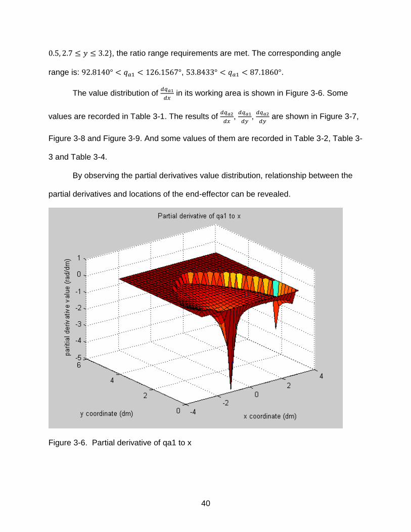
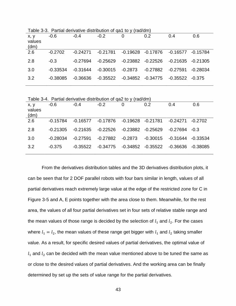
The value distribution of
in its working area is shown in Figure 3-6. Some
values are recorded in Table 3-1. The results of
,
,
are shown in Figure 3-7,
Figure 3-8 and Figure 3-9. And some values of them are recorded in Table 3-2, Table 3-
3 and Table 3-4.
By observing the partial derivatives value distribution, relationship between the
partial derivatives and locations of the end-effector can be revealed.
Figure 3-6. Partial derivative of qa1 to x

41
Figure 3-7. Partial derivative of qa1 to y
Figure 3-8. Partial derivative of qa2 to x
42
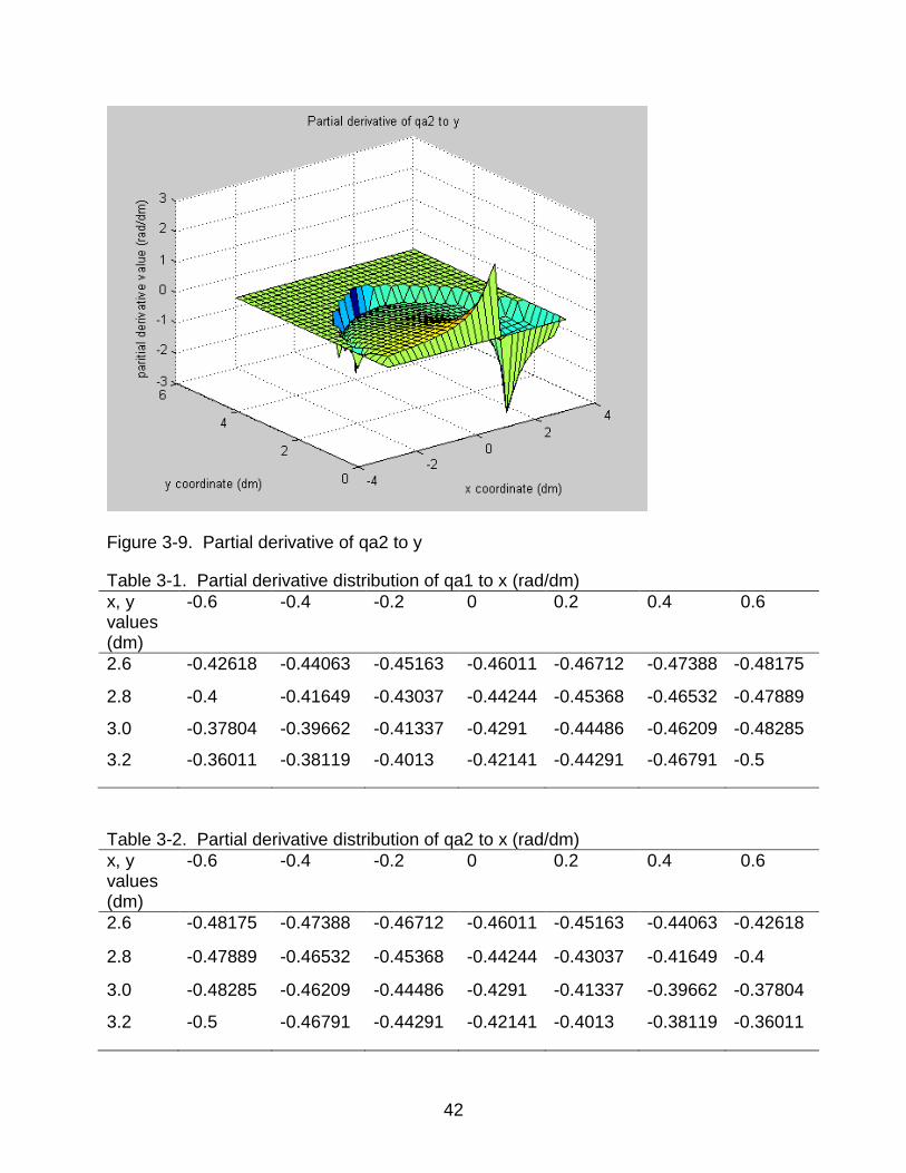
Figure 3-9. Partial derivative of qa2 to y
Table 3-1. Partial derivative distribution of qa1 to x (rad/dm)
x, y values (dm)
-0.6 -0.4 -0.2 0 0.2 0.4 0.6
2.6 -0.42618 -0.44063 -0.45163 -0.46011 -0.46712 -0.47388 -0.48175
2.8 -0.4 -0.41649 -0.43037 -0.44244 -0.45368 -0.46532 -0.47889
3.0 -0.37804 -0.39662 -0.41337 -0.4291 -0.44486 -0.46209 -0.48285
3.2 -0.36011 -0.38119 -0.4013 -0.42141 -0.44291 -0.46791 -0.5
Table 3-2. Partial derivative distribution of qa2 to x (rad/dm)
x, y values (dm)
-0.6 -0.4 -0.2 0 0.2 0.4 0.6
2.6 -0.48175 -0.47388 -0.46712 -0.46011 -0.45163 -0.44063 -0.42618
2.8 -0.47889 -0.46532 -0.45368 -0.44244 -0.43037 -0.41649 -0.4
3.0 -0.48285 -0.46209 -0.44486 -0.4291 -0.41337 -0.39662 -0.37804
3.2 -0.5 -0.46791 -0.44291 -0.42141 -0.4013 -0.38119 -0.36011
43
Table 3-3. Partial derivative distribution of qa1 to y (rad/dm)
x, y values (dm)
-0.6 -0.4 -0.2 0 0.2 0.4 0.6
2.6 -0.2702 -0.24271 -0.21781 -0.19628 -0.17876 -0.16577 -0.15784
2.8 -0.3 -0.27694 -0.25629 -0.23882 -0.22526 -0.21635 -0.21305
3.0 -0.33534 -0.31644 -0.30015 -0.2873 -0.27882 -0.27591 -0.28034
3.2 -0.38085 -0.36636 -0.35522 -0.34852 -0.34775 -0.35522 -0.375
Table 3-4. Partial derivative distribution of qa2 to y (rad/dm)
x, y values (dm)
-0.6 -0.4 -0.2 0 0.2 0.4 0.6
2.6 -0.15784 -0.16577 -0.17876 -0.19628 -0.21781 -0.24271 -0.2702
2.8 -0.21305 -0.21635 -0.22526 -0.23882 -0.25629 -0.27694 -0.3
3.0 -0.28034 -0.27591 -0.27882 -0.2873 -0.30015 -0.31644 -0.33534
3.2 -0.375 -0.35522 -0.34775 -0.34852 -0.35522 -0.36636 -0.38085
From the derivatives distribution tables and the 3D derivatives distribution plots, it
can be seen that for 2 DOF parallel robots with four bars similar in length, values of all
partial derivatives reach extremely large value at the edge of the restricted zone for C in
Figure 3-5 and A, E points together with the area close to them. Meanwhile, for the rest
area, the values of all four partial derivatives set in four sets of relative stable range and
the mean values of those range is decided by the selection of and . For the cases
where , the mean values of these range get bigger with and taking smaller
value. As a result, for specific desired values of partial derivatives, the optimal value of
and can be decided with the mean value mentioned above to be tuned the same as
or close to the desired values of partial derivatives. And the working area can be finally
determined by set up the sets of value range for the partial derivatives.
44
3.3 Modeling for the 2 DOF Parallel Robot
3.3.1 Dynamics Model for the 2 DOF Parallel Robot
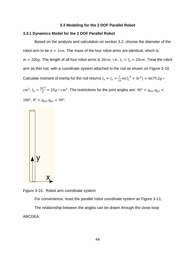
Based on the analysis and calculation on section 3.2, choose the diameter of the
robot arm to be . The mass of the four robot arms are identical, which is:
. The length of all four robot arms is , i.e., . Treat the robot
arm as thin rod, with a coordinate system attached to the rod as shown on Figure 3-10.
Calculate moment of inertia for the rod returns
(
)
,
. The restrictions for the joint angles are:
, .
Figure 3-10. Robot arm coordinate system
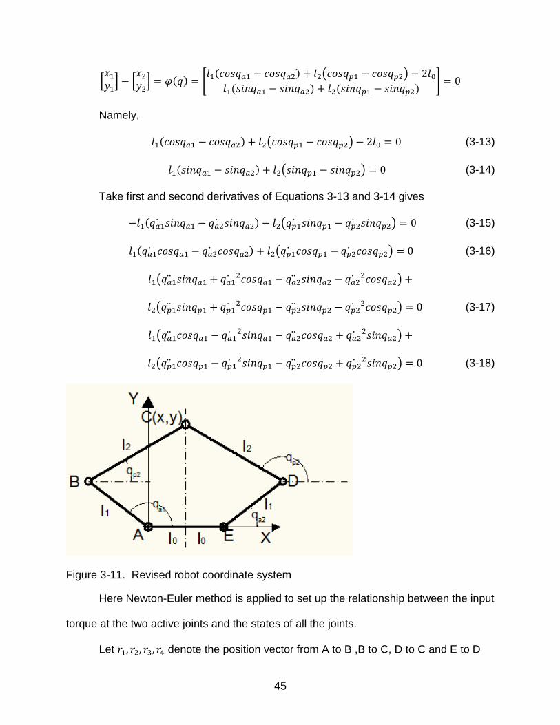
For convenience, reset the parallel robot coordinate system as Figure 3-11.
The relationship between the angles can be drawn through the close-loop
ABCDEA:
45
[
] [
] ( ) [
( ) ( ) ( ) ( )
]
Namely,
( ) ( ) (3-13)
( ) ( ) (3-14)
Take first and second derivatives of Equations 3-13 and 3-14 gives
( ) ( ) (3-15)
( ) ( ) (3-16)
(
)
(
) (3-17)
(
)
(
) (3-18)
Figure 3-11. Revised robot coordinate system
Here Newton-Euler method is applied to set up the relationship between the input
torque at the two active joints and the states of all the joints.
Let denote the position vector from A to B ,B to C, D to C and E to D
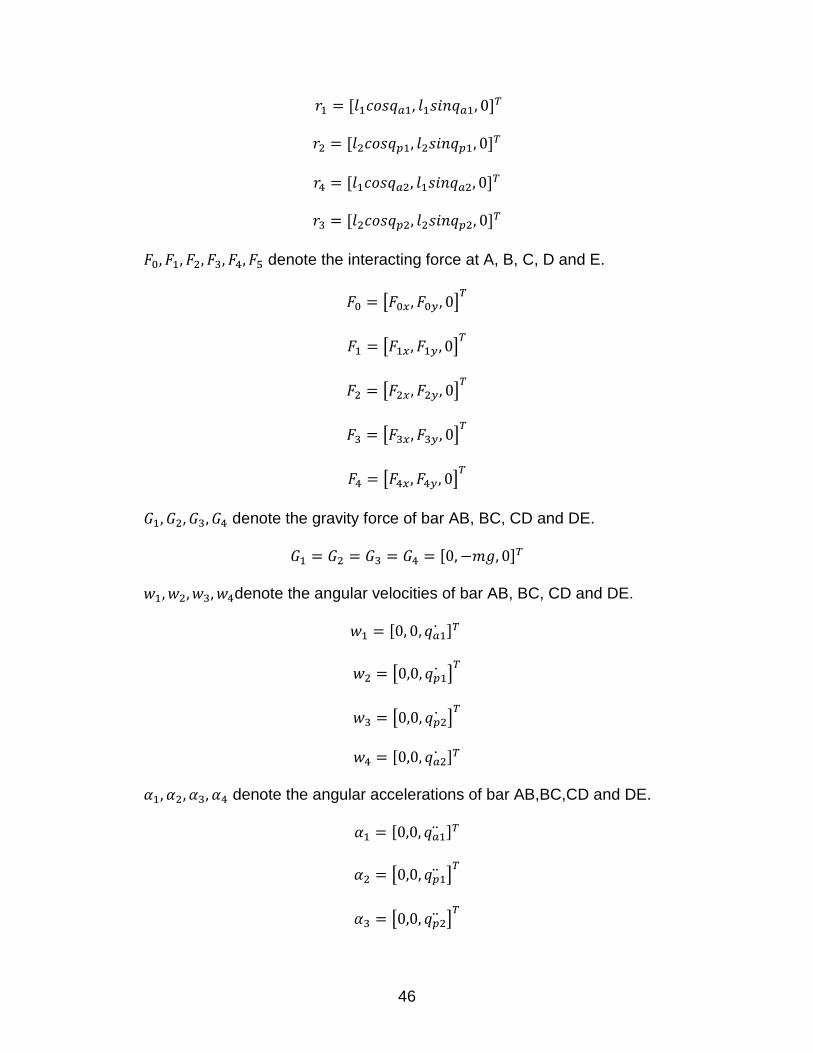
46
denote the interacting force at A, B, C, D and E.
[ ]
[ ]
[ ]
[ ]
[ ]
denote the gravity force of bar AB, BC, CD and DE.
denote the angular velocities of bar AB, BC, CD and DE.
[ ]
[ ]
denote the angular accelerations of bar AB,BC,CD and DE.
[ ]
[ ]
47
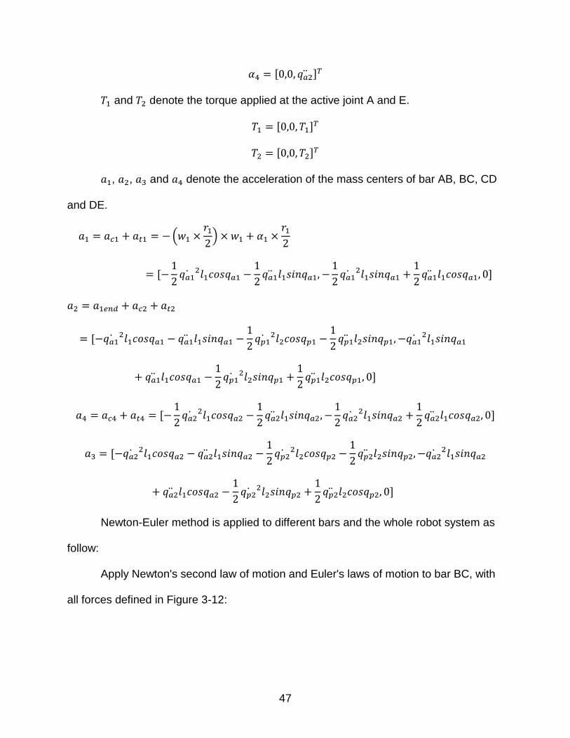
and denote the torque applied at the active joint A and E.
, , and denote the acceleration of the mass centers of bar AB, BC, CD
and DE.
( )
Newton-Euler method is applied to different bars and the whole robot system as
follow:
Apply Newton's second law of motion and Euler's laws of motion to bar BC, with
all forces defined in Figure 3-12:
48
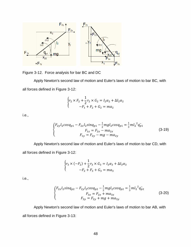
Figure 3-12. Force analysis for bar BC and DC
Apply Newton's second law of motion and Euler's laws of motion to bar BC, with
all forces defined in Figure 3-12:
{
i.e.,
{
(3-19)
Apply Newton's second law of motion and Euler's laws of motion to bar CD, with
all forces defined in Figure 3-12:
{ ( )
i.e.,
{
(3-20)
Apply Newton's second law of motion and Euler's laws of motion to bar AB, with
all forces defined in Figure 3-13:
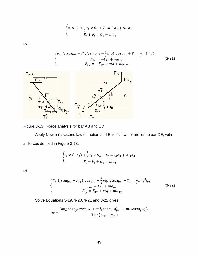
49
{
i.e.,
{
(3-21)
Figure 3-13. Force analysis for bar AB and ED
Apply Newton's second law of motion and Euler's laws of motion to bar DE, with
all forces defined in Figure 3-13:
{ ( )
i.e.,
{
(3-22)
Solve Equations 3-19, 3-20, 3-21 and 3-22 gives
( )

50
( )
( )
(3-23)
(3-24)
where
( )
( )
( )
( )
( )
( )
( ( ))
( )
( )
( )
( )
( )
( )
( )
( ( ) )
( )
The relationship between the input torques and the angular states is therefore
shown in Equations 3-23 and 3-24. Combined Equations 3-23, 3-24 with Equations 3-
17, 3-18 returns the dynamic equation of the 2 DOF parallel robot.
( ) ( ) ( )
51
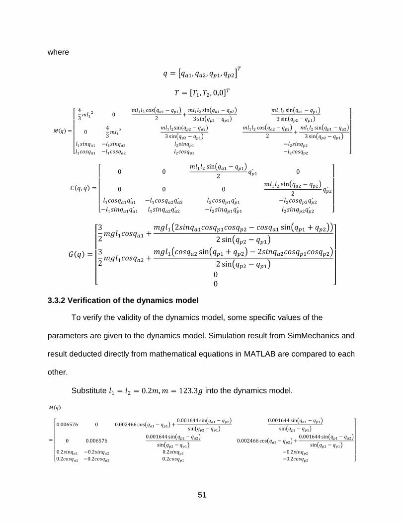
where
[ ]
( )
[
( )
( )
( )
( )
( )
( )
( )
( )
( )
( )
]
( )
[
( )
( )
]
( )
[
( ( ))
( )
( ( ) )
( )
]
3.3.2 Verification of the dynamics model
To verify the validity of the dynamics model, some specific values of the
parameters are given to the dynamics model. Simulation result from SimMechanics and
result deducted directly from mathematical equations in MATLAB are compared to each
other.
Substitute into the dynamics model.
( )
[ ( )
( )
( )
( )
( )
( )
( ) ( )
( )
( )
]

52
( )
[
( )
( )
]
( )
[
( ( ))
( )
( ( ) )
( )
]
As verification for the accuracy of the mathematical model, the dynamic
characteristics of mathematical model will be compared to the results from the
SimMechanics model in Figure 3-14.
Figure 3-14. SimMechanics model for the 2 DOF parallel robot
53
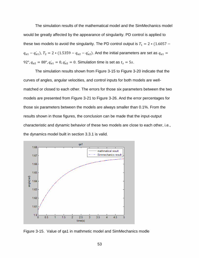
The simulation results of the mathematical model and the SimMechanics model
would be greatly affected by the appearance of singularity. PD control is applied to
these two models to avoid the singularity. The PD control output is (
), ( ). And the initial parameters are set as
. Simulation time is set as .
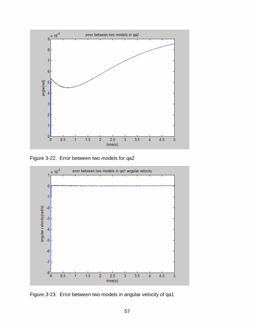
The simulation results shown from Figure 3-15 to Figure 3-20 indicate that the
curves of angles, angular velocities, and control inputs for both models are well-
matched or closed to each other. The errors for those six parameters between the two
models are presented from Figure 3-21 to Figure 3-26. And the error percentages for
those six parameters between the models are always smaller than 0.1%. From the
results shown in those figures, the conclusion can be made that the input-output
characteristic and dynamic behavior of these two models are close to each other, i.e.,
the dynamics model built in section 3.3.1 is valid.
Figure 3-15. Value of qa1 in mathmetic model and SimMechanics modle

54
Figure 3-16. Value of qa2 in mathematical model and SimMechanics model
Figure 3-17. Angular velocity of qa1 in mathematical model and SimMechanics model
55
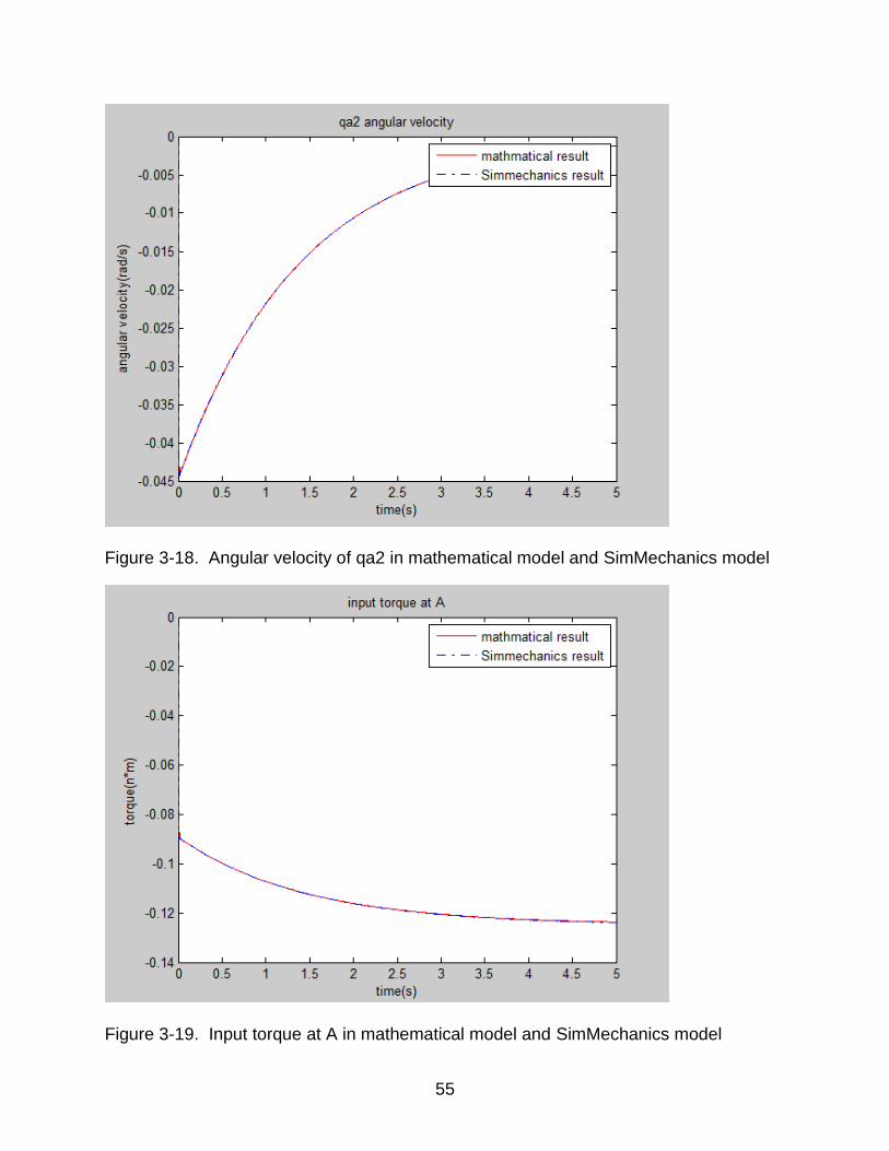
Figure 3-18. Angular velocity of qa2 in mathematical model and SimMechanics model
Figure 3-19. Input torque at A in mathematical model and SimMechanics model
56
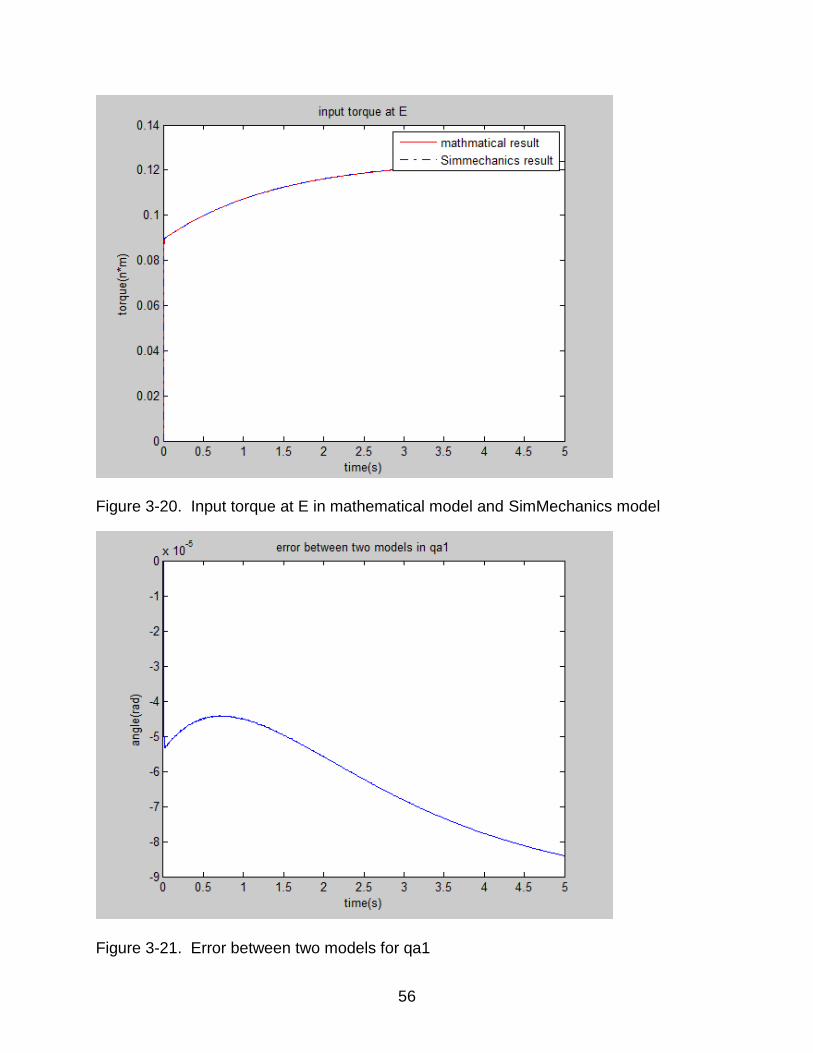
Figure 3-20. Input torque at E in mathematical model and SimMechanics model
Figure 3-21. Error between two models for qa1
57
Figure 3-22. Error between two models for qa2
Figure 3-23. Error between two models in angular velocity of qa1

58
Figure 3-24. Error between two models in angular velocity of qa2
Figure 3-25. Error between two models for input torque at A
59
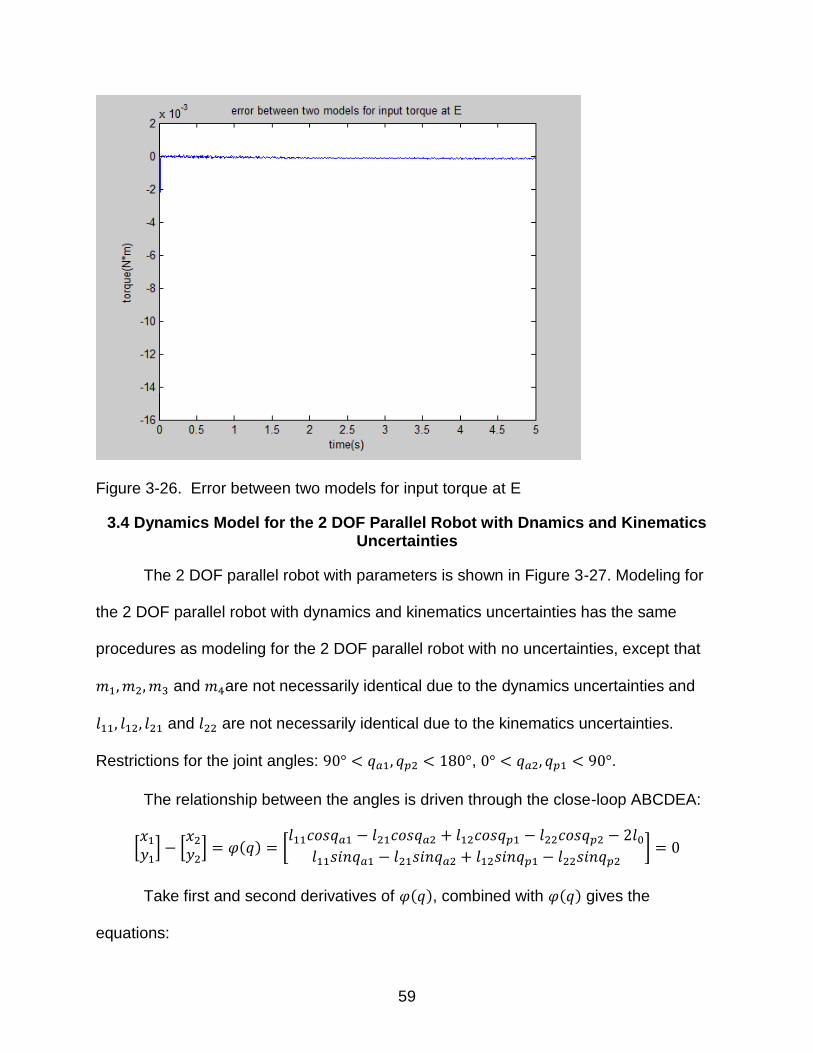
Figure 3-26. Error between two models for input torque at E
3.4 Dynamics Model for the 2 DOF Parallel Robot with Dnamics and Kinematics Uncertainties
The 2 DOF parallel robot with parameters is shown in Figure 3-27. Modeling for
the 2 DOF parallel robot with dynamics and kinematics uncertainties has the same
procedures as modeling for the 2 DOF parallel robot with no uncertainties, except that
and are not necessarily identical due to the dynamics uncertainties and
and are not necessarily identical due to the kinematics uncertainties.
Restrictions for the joint angles: , .
The relationship between the angles is driven through the close-loop ABCDEA:
[
] [
] ( ) [
]
Take first and second derivatives of ( ), combined with ( ) gives the
equations:
60
( ) (
) (
) (
) (3-25)
( ) (
) (
) (
) (3-26)
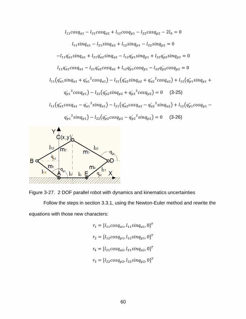
Figure 3-27. 2 DOF parallel robot with dynamics and kinematics uncertainties
Follow the steps in section 3.3.1, using the Newton-Euler method and rewrite the
equations with those new characters:
61
( )
[
]
[
]
[
]
[
]
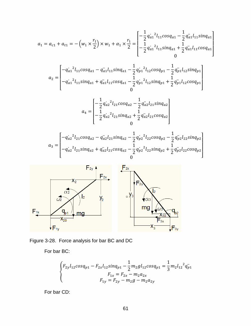
Figure 3-28. Force analysis for bar BC and DC
For bar BC:
{
For bar CD:
62
{
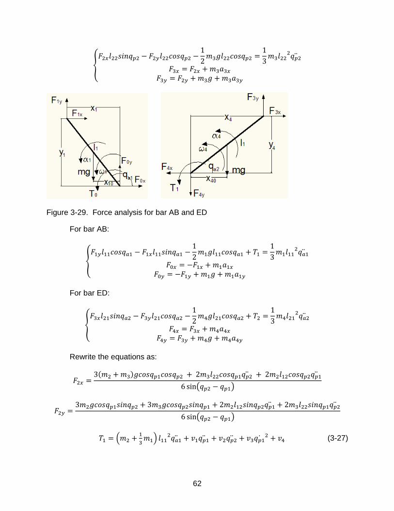
Figure 3-29. Force analysis for bar AB and ED
For bar AB:
{
For bar ED:
{
Rewrite the equations as:
( )
( )
( )
(
)
(3-27)

63
(
)
(3-28)
where
( )
( )
( )
( )
( )
( )
( ( ) ( )
( )
)
( )
( )
( )
( )
( )
( )
( ( ) ( )
( )
)
Combine Equations 3-27 and 3-28 gives
[
] [
] [
] [
] (3-29)
where

64
[(
)
(
)
]
[
( )
( )
( )
( )
( )
( )
( )
( )
( )
( ) ]
[
( )
( )
]
[ (
( ) ( )
( )
)
( ( ) ( )
( )
)
]
Substitute and with and in Equation 3-29
[
] [
]
where
[ ( ) ( ) ( ) ( )
]
[ ( ) ( ) ( ) ( )
]
[ (
( ) ( )
( )
)
( ( ) ( )
( )
)
]
with
( ) (
)
( )(
( ) ( )
( )
( ))
( )
( )
65
( )
( )(
( ) ( )
( ) ( )
( ))
( ) ( )
( )
( ) ( ) ( )
( )
( )(
( ) ( )
( ) ( )
( ))
( ) (
)
( )
( )
( )(
( ) ( )
( )
( ))
( )
( )( ( ) ( ) ( ))
( ( ) ( ))
( )
where
( ) (
( ) ( )
( ) ( )
( ))
( ) ( ( ) ( )
( )
( ) ( )
( ))
( ) ( ( ) ( )
( )
( ) ( )
( ))
( ) ( ) ( ) ( )
( ) ( ) ( ) ( ) ( )
( )
( )( ( ) ( ) ( ))
( ( ) ( ))
( )
( ) (
( ) ( )
( ) ( )
( ))
( ) ( ( ) ( )
( )
( ) ( )
( ))
66
( ) ( ( ) ( )
( )
( ) ( )
( ))
( ) ( ) ( ) ( )
( ) ( ) ( )
( ) ( ) ( )
( ) ( ( ) ( ))
( )
( )( ( ) ( ) ( ))
( ) ( ) ( ) ( )
( ) ( ) ( ) ( )
( ) ( )
( ) (
( ) ( )
( ) ( )
( ))
( ) ( ( ) ( )
( )
( ) ( )
( ))
( ) ( ( ) ( )
( )
( ) ( )
( ))
( )
( ( ) ( ))
( )
( )( ( ) ( ) ( ))
( ) ( ) ( ) ( )
( ) ( ) ( ) ( ) ( )
67
( ) (
( ) ( )
( ) ( )
( ))
( ) ( ( ) ( )
( )
( ) ( )
( ))
( ) ( ( ) ( )
( )
( ) ( )
( ))
68
CHAPTER 4 CONTROL SYSTEM DESIGN FOR 2 DOF PARALLEL ROBOT
4.1 Adaptive Backstepping Controller for the 2 DOF Parallel Robot Model with Uncertainties
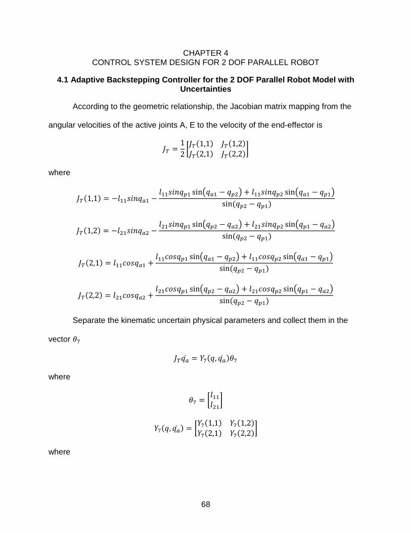
According to the geometric relationship, the Jacobian matrix mapping from the
angular velocities of the active joints A, E to the velocity of the end-effector is
[ ( ) ( )
( ) ( )]
where
( ) ( ) ( )
( )
( ) ( ) ( )
( )
( ) ( ) ( )
( )
( ) ( ) ( )
( )
Separate the kinematic uncertain physical parameters and collect them in the
vector
( )
where
[
]
( ) [ ( ) ( )
( ) ( )]
where

69
( ) ( ( ) ( )
( ))
( ) ( ( ) ( )
( ))
( ) ( ( ) ( )
( ))
( ) ( ( ) ( )
( ))
Estimate of
[ ( ) ( )
( ) ( )]
where
( ) ( ) ( )
( )
( ) ( ) ( )
( )
( ) ( ) ( )
( )
( ) ( ) ( )
( )
From the analysis in section 3.4, the dynamic model for 2DOF Parallel Robot
ignoring friction would be
[
] [
]
According to Property3
( ) ( ) ( ) ( )
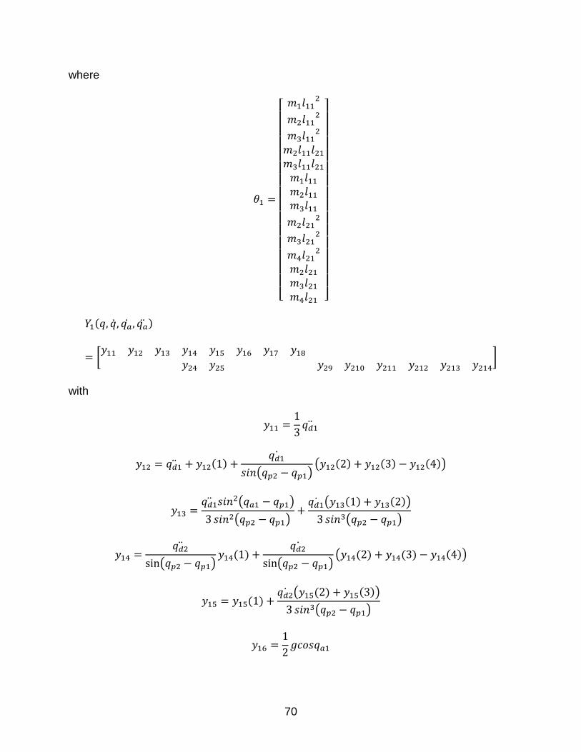
70
where
[
]
( )
[
]
with
( )
( )( ( ) ( ) ( ))
( )
( )
( ( ) ( ))
( )
( ) ( )
( )( ( ) ( ) ( ))
( ) ( ( ) ( ))
( )
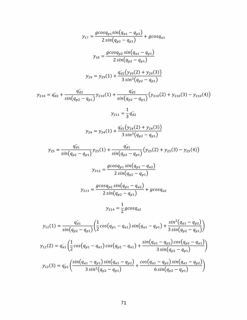
71
( )
( )
( )
( )
( ) ( ( ) ( ))
( )
( ) ( )
( )( ( ) ( ) ( ))
( ) ( ( ) ( ))
( )
( ) ( )
( )( ( ) ( ) ( ))
( )
( )
( )
( )
( )
( )(
( ) ( )
( )
( ))
( ) (
( ) ( )
( ) ( )
( ))
( ) ( ( ) ( )
( )
( ) ( )
( ))
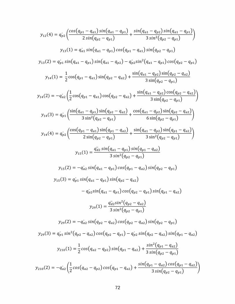
72
( ) ( ( ) ( )
( )
( ) ( )
( ))
( ) ( ) ( ) ( )
( ) ( ) ( ) ( ) ( )
( )
( ) ( )
( ) ( )
( )
( ) (
( ) ( )
( ) ( )
( ))
( ) ( ( ) ( )
( )
( ) ( )
( ))
( ) ( ( ) ( )
( )
( ) ( )
( ))
( ) ( ) ( )
( )
( ) ( ) ( ) ( )
( ) ( ) ( )
( ) ( ) ( )
( ) ( )
( )
( ) ( ) ( ) ( )
( ) ( ) ( ) ( ) ( )
( )
( ) ( )
( )
( )
( ) (
( ) ( )
( ) ( )
( ))

73
( ) ( ( ) ( )
( )
( ) ( )
( ))
( ) ( ( ) ( )
( )
( ) ( )
( ))
( ) ( ) ( )
( )
( ) ( ) ( ) ( )
( ) ( ) ( ) ( )
( ) ( )
( )
( ) ( )
( ) ( )
( )
( ) (
( ) ( )
( ) ( )
( ))
( ) ( ( ) ( )
( )
( ) ( )
( ))
( ) ( ( ) ( )
( )
( ) ( )
( ))
The actual structure parameters of the 2-DOF parallel robot in the simulation are
designed as
(a)
For the implementation, the parameter estimates are initialized as
(b)
The desired the point is designed as
74
[
]
The desired trajectory is designed as
[
]
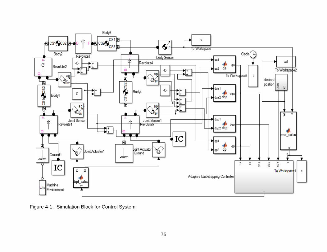
Bring those values into expressions of the dynamics model. With the assistance
of MATLAB SimMechanics, the simulation model of the 2-DOF parallel robot with
structure parameters in (a) controlled by the adaptive backstepping controller using
initial estimate parameters in (b) is built up and shown in Figure 4-1.
4.2 Simulation Result and Discussion
In this section, two types of tracking control, set point tracking control and
trajectory tracking control, are implemented. For the set point tracking control, the
assignment for the controller is to adjust the input torque on the active joints so that the
end-effector could eventually reach the destination point. For the trajectory tracking
control, the controller manages the input torque on the active joints with the goal to
follow the desired trajectory. As a contrast, set point control and trajectory control using
the only backsteppping controller carried out on the same 2-DOF parallel robot.
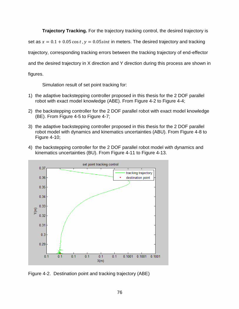
Set Point Tracking. For the set point tracking control, the desired point is given as
( ) . The destination point and tracking trajectory, tracking errors between the
end-effector and the destination point in X direction and Y direction during this process
are displayed in figures.
75
Figure 4-1. Simulation Block for Control System
76
Trajectory Tracking. For the trajectory tracking control, the desired trajectory is
set as in meters. The desired trajectory and tracking
trajectory, corresponding tracking errors between the tracking trajectory of end-effector
and the desired trajectory in X direction and Y direction during this process are shown in
figures.
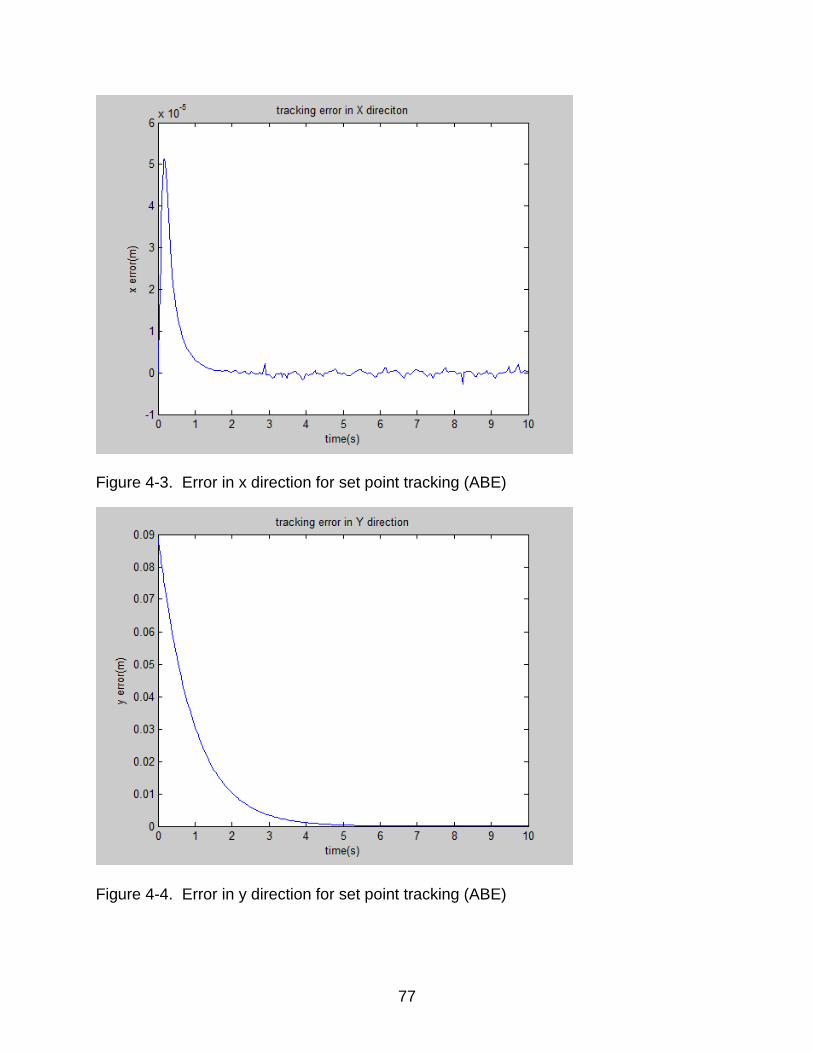
Simulation result of set point tracking for:
1) the adaptive backstepping controller proposed in this thesis for the 2 DOF parallel robot with exact model knowledge (ABE). From Figure 4-2 to Figure 4-4;
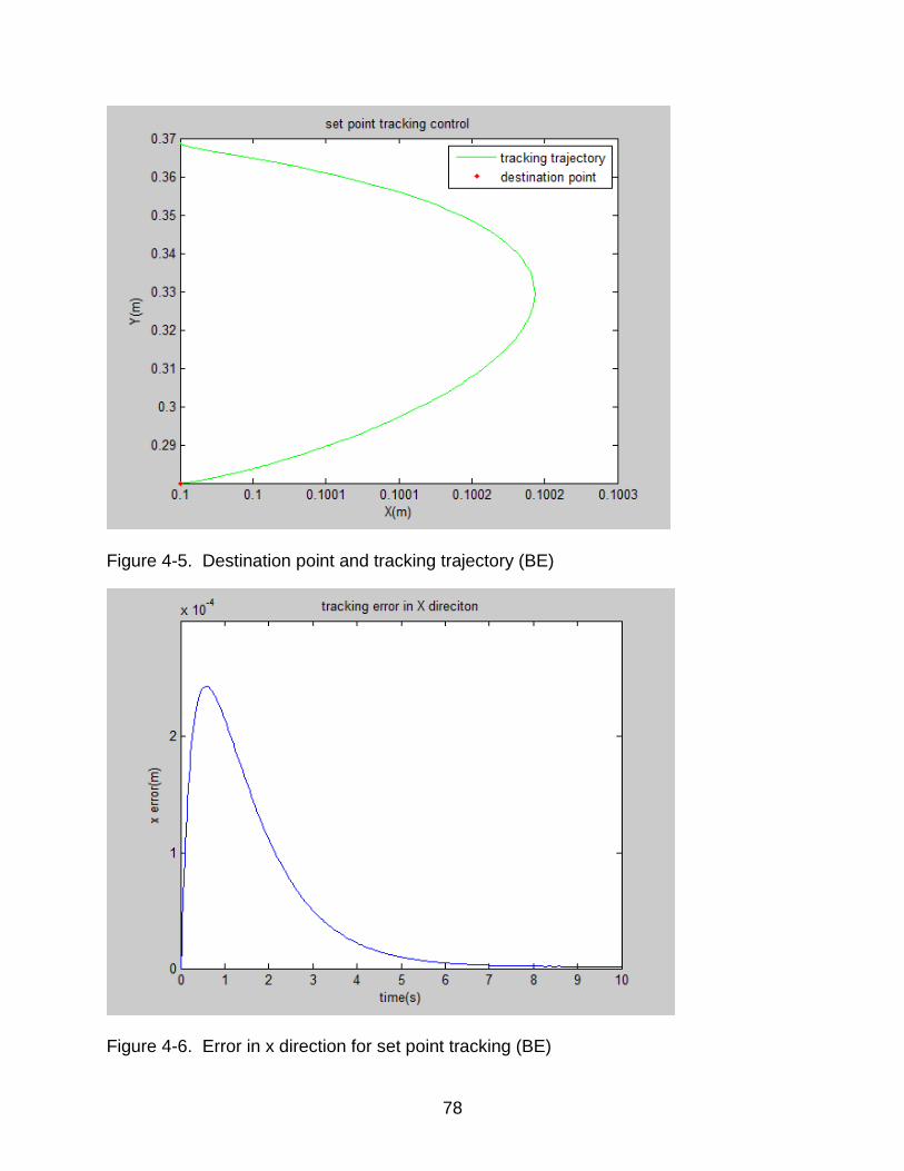
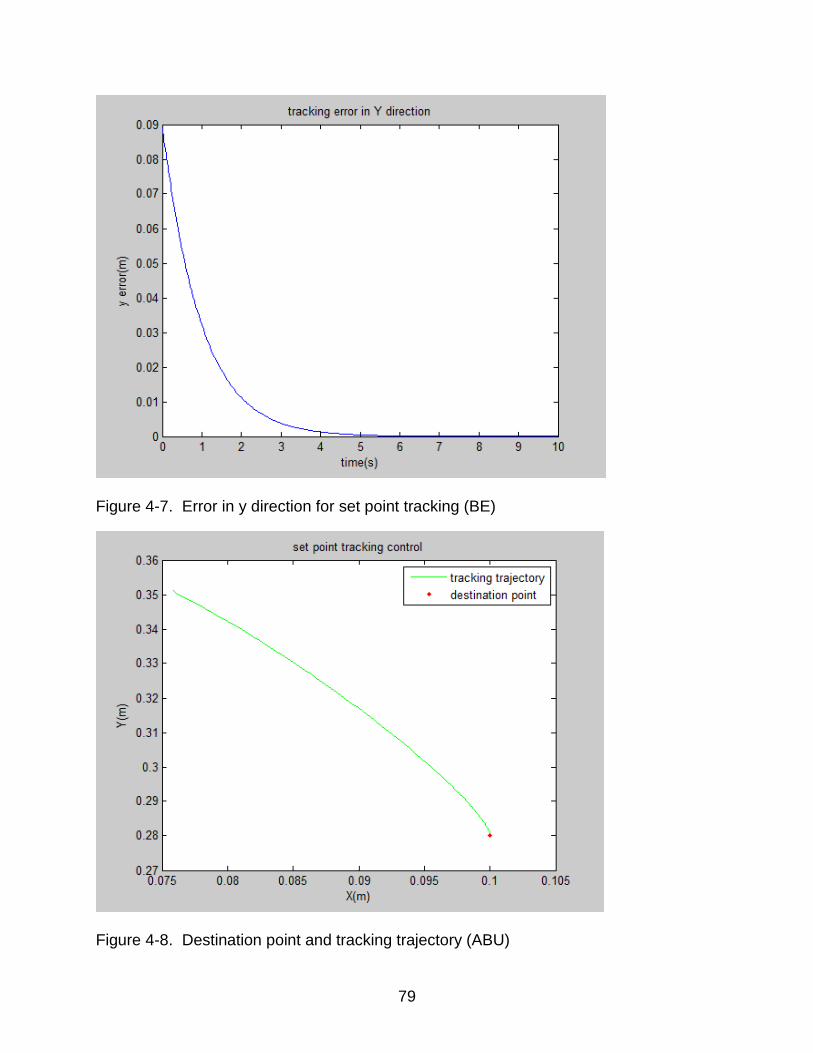
2) the backstepping controller for the 2 DOF parallel robot with exact model knowledge (BE). From Figure 4-5 to Figure 4-7;
3) the adaptive backstepping controller proposed in this thesis for the 2 DOF parallel robot model with dynamics and kinematics uncertainties (ABU). From Figure 4-8 to Figure 4-10;
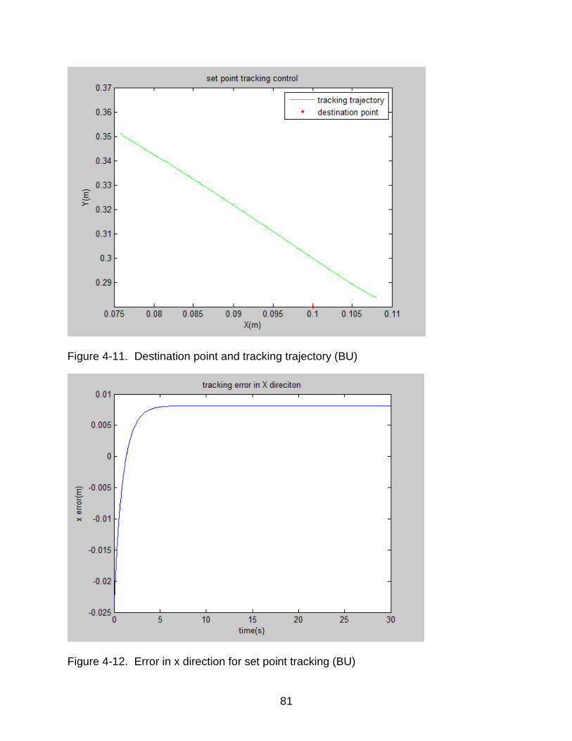
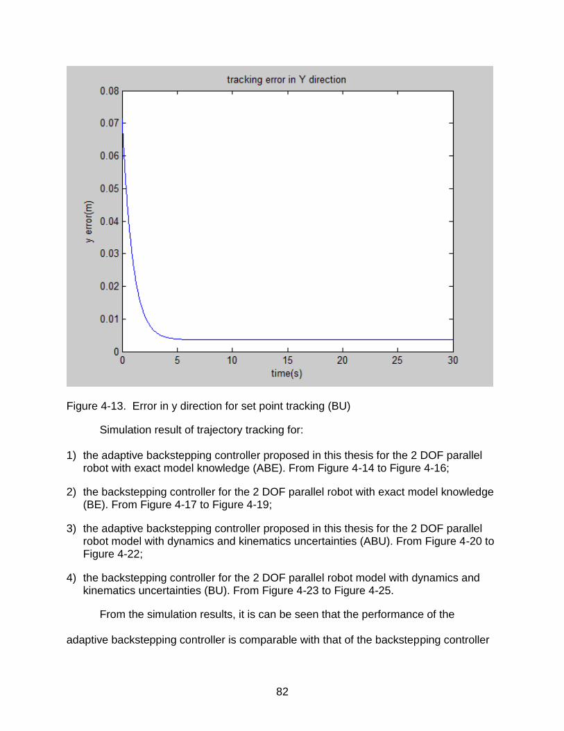
4) the backstepping controller for the 2 DOF parallel robot model with dynamics and kinematics uncertainties (BU). From Figure 4-11 to Figure 4-13.
Figure 4-2. Destination point and tracking trajectory (ABE)
77
Figure 4-3. Error in x direction for set point tracking (ABE)
Figure 4-4. Error in y direction for set point tracking (ABE)
78
Figure 4-5. Destination point and tracking trajectory (BE)
Figure 4-6. Error in x direction for set point tracking (BE)
79
Figure 4-7. Error in y direction for set point tracking (BE)
Figure 4-8. Destination point and tracking trajectory (ABU)

80
Figure 4-9. Error in x direction for set point tracking (ABU)
Figure 4-10. Error in y direction for set point tracking (ABU)
81
Figure 4-11. Destination point and tracking trajectory (BU)
Figure 4-12. Error in x direction for set point tracking (BU)
82
Figure 4-13. Error in y direction for set point tracking (BU)
Simulation result of trajectory tracking for:
1) the adaptive backstepping controller proposed in this thesis for the 2 DOF parallel robot with exact model knowledge (ABE). From Figure 4-14 to Figure 4-16;
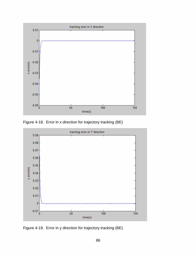
2) the backstepping controller for the 2 DOF parallel robot with exact model knowledge (BE). From Figure 4-17 to Figure 4-19;
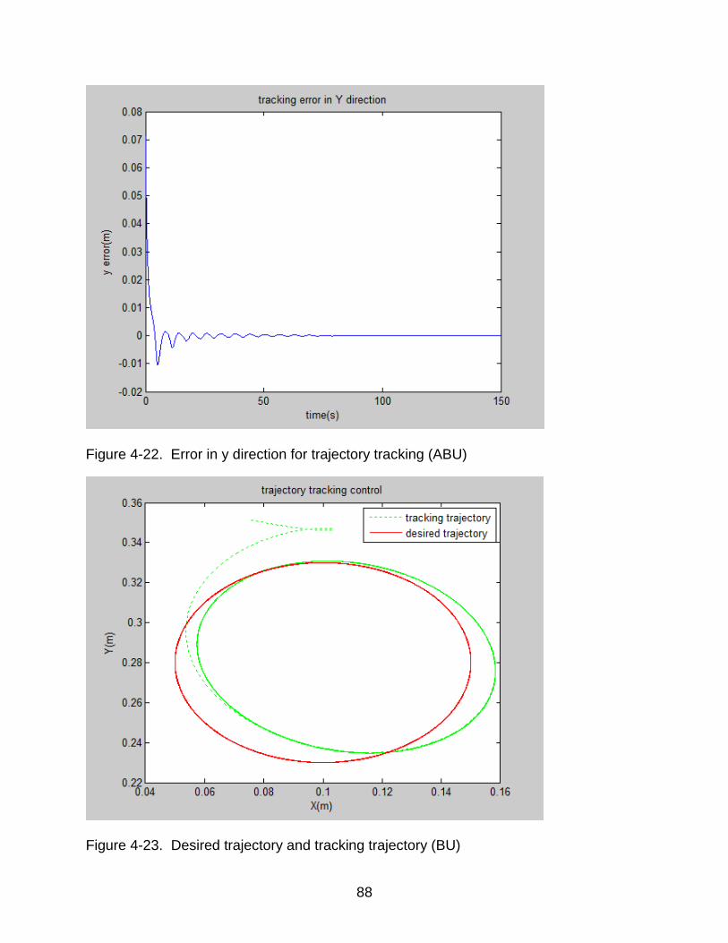
3) the adaptive backstepping controller proposed in this thesis for the 2 DOF parallel robot model with dynamics and kinematics uncertainties (ABU). From Figure 4-20 to Figure 4-22;
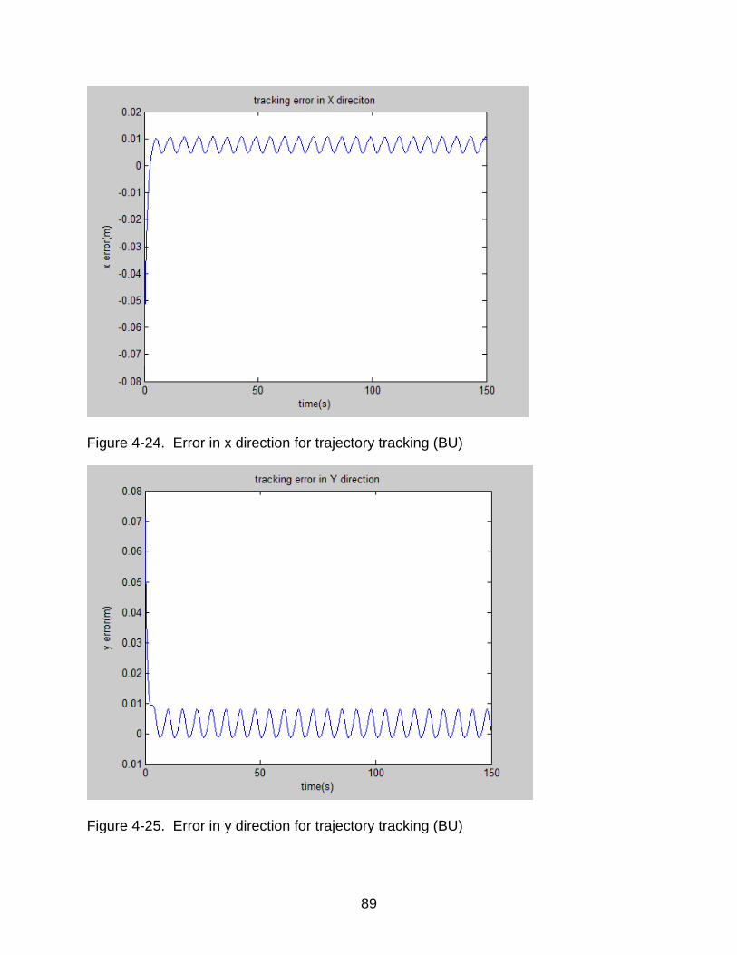
4) the backstepping controller for the 2 DOF parallel robot model with dynamics and kinematics uncertainties (BU). From Figure 4-23 to Figure 4-25.
From the simulation results, it is can be seen that the performance of the
adaptive backstepping controller is comparable with that of the backstepping controller
83
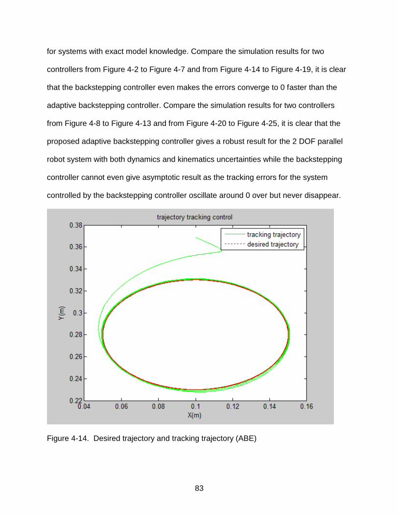
for systems with exact model knowledge. Compare the simulation results for two
controllers from Figure 4-2 to Figure 4-7 and from Figure 4-14 to Figure 4-19, it is clear
that the backstepping controller even makes the errors converge to 0 faster than the
adaptive backstepping controller. Compare the simulation results for two controllers
from Figure 4-8 to Figure 4-13 and from Figure 4-20 to Figure 4-25, it is clear that the
proposed adaptive backstepping controller gives a robust result for the 2 DOF parallel
robot system with both dynamics and kinematics uncertainties while the backstepping
controller cannot even give asymptotic result as the tracking errors for the system
controlled by the backstepping controller oscillate around 0 over but never disappear.
Figure 4-14. Desired trajectory and tracking trajectory (ABE)

84
Those results fit well with the corresponding theory. Because the backstepping
controller used as a contrast is exact model based controller, it does not involve the
estimators. For exact model system, those controllers without the ‘estimator’ could
instantly give the required or desired control output on the system to reach the
destination in a more efficient and faster way. And that is one of the advantages for the
exact model knowledge based controller. Though giving inspiring control result for exact
model system, those controllers act badly when no exact model knowledge about the
system is available. Therefore, for the uncertain model cases, the backstepping
controller cannot give asymptotic tracking results. As for the proposed adaptive
backstepping controller, the estimator in the controller can adjust to the dynamics and
kinematics uncertainties through self-adaptive process, thus drive the errors to 0.
Figure 4-15. Error in x direction for trajectory tracking (ABE)

85
Figure 4-16. Error in y direction for trajectory tracking (ABE)
Figure 4-17. Desired trajectory and tracking trajectory (BE)
86
Figure 4-18. Error in x direction for trajectory tracking (BE)
Figure 4-19. Error in y direction for trajectory tracking (BE)

87
Figure 4-20. Desired trajectory and tracking trajectory (ABU)
Figure 4-21. Error in x direction for trajectory tracking (ABU)
88
Figure 4-22. Error in y direction for trajectory tracking (ABU)
Figure 4-23. Desired trajectory and tracking trajectory (BU)
89
Figure 4-24. Error in x direction for trajectory tracking (BU)
Figure 4-25. Error in y direction for trajectory tracking (BU)
90
CHAPTER 5 CONCLUSION AND FUTURE WORK
The proposed adaptive backstepping controller could well address the issue of
precise position control or tracking control for the 2 DOF parallel robots with dynamics
and kinematics uncertainties. Actually, from the analysis in section 2, it is not hard to
realize that the proposed adaptive backstepping controller could achieve precise
position control or tracking control for all parallel robot connected only by revolute joints.
This research opens up to new challenges. One of them is to explore the
influence of the coefficients on the control result. The influence of
on the control result is quite different. From some sample tests, it
appears has a greater influence on the control result than the other coefficients.
Further work could be done to reveal a relatively more complete relationship between
those coefficients and the control result. This is a very useful aspect as it provides
guidelines on how to tune those coefficients to get different types of desired results.
In addition, the coverage of the proposed adaptive controller can be extended.
The kinematics analysis in section 2 is limited to parallel robot connected only by
revolute joints. But this restriction is not final. Similar analysis can be applied on other
sorts of parallel robot.
91
REFERENCES
1. Christian Smith and Henrik I. Christensen, “Robot Manipulators Constructing a High-Performance Robot from Commercially Available Parts,” Robotics & Automation Magazine. 16, 75–83 (2009). 2. Carl D. Crane, III and Joseph Duffy, Kinematic Analysis of Robot Manipulators (Cambridge University Press, New York, US, 1998). 3. Wei Wei Shang, Shuang Cong, Ze Xiang Li and Shi Long Jiang, “Augmented Nonlinear PD Controller for a Redundantly Actuated Parallel Manipulator,” Advanced Robotics. 23, 1725–1742 (2009). 4. Hui Cheng, Yiu-Kuen Yiu and Zexiang Li, “Dynamics and Control of Redundantly Actuated Parallel Manipulators,” Transactions on Mechatronics. 8, 483–491 (2003). 5. Jin Qinglong and Chen Wenjie, “Adaptive Control of 6-DOF Parallel Manipulator,” 30th Chinese Control Conference (2011) pp. 2440–2445. 6. Meysar Zeinali and Leila Notash, “Adaptive sliding mode control with uncertainty estimator for robot manipulators,” Mechanism and Machine Theory. 45, 80–90 (2010). 7. Jinkun Liu and Xinhua Wang, Advanced Sliding Mode Control for Mechanical Systems (Tsinghua University Press, Beijing, China, 2011). 8. C. C. Cheah, C. Liu and J. J. E. Slotine, “Adaptive Jacobian tracking control of robots with uncertainties in kinematic, dynamic and actuator models,” IEEE Transactions on Automatic Control. 51, 1024–1029 (2006). 9. C. C. Cheah, C. Liu and J. J. E. Slotine, “Approximate Jacobian adaptive control for robot manipulators,” IEEE International Confannee on Robtics &Automation. 3, 3075–3080 (2004). 10. Mohammad Reza Soltanpour, Jafaar Khalilpour and Mahmoodreza Soltani, “Robust Nonlinear Control of Robot Manipulator With Uncertainties in Kinematics Dynamics and Actuator Models,” International Journal of Innovative Computing, Information and Control. 8, 5487–5498 (2012). 11. M. Ahmadipour, A. Khayatian and M. Dehghani, “Adaptive Backstepping Control of Rigid Link Electrically Driven Robots with Uncertain Kinematics and Dynamics,” 2nd International Conference on Control, Instrumentation and Automation (2011) pp. 911–916. 12. Stefan Dutré, Herman Bruyninckx and Joris De Schutter, “The analytical Jacobian and its derivative for a parallel manipulator,” IEEE International Conference on Robotics and Automation, Albuquerque. 4, 2961–2966( 1997).
92
13. Tien Dung Le, Hee-Jun Kang and Young-Shick Ro, “Kinematic and Singularity Analysis of Symmetrical 2 DOF Parallel Manipulators,” 7th International Forum on Strategic Technology (2012) pp. 1 – 4. 14. W. E. Dixon, “Adaptive regulation of amplitude limited robot manipulators with uncertain kinematics and dynamics,” Proc. Amer. Control Conf. (2004) pp. 3844–3939. 15. Wenbin Deng, Jae-Won Lee and Hyuk-Jin Lee, “Kinematics Simulation and Control of a New 2 DOF Parallel Mechanism Based on Matlab/SimMechanics,” 2009 ISECS International Colloquium on Computing, Communication, Control, and Management. 3,233 – 236 (2009).
93
BIOGRAPHICAL SKETCH
Jing Zou was born in Nanchang, China, in the year 1989. He received a
bachelor’s degree in mechanical engineering from the Huazhong University of Science
and Technology in Wuhan, China, in June, 2012. He joined the master’s program in the
Mechanical and Aerospace Engineering Department at the University of Florida in
August 2012 and received his MS degree in May 2014.