design of a wide-angle biconical antenna for wideband communications … · progress in...

Progress In Electromagnetics Research B, Vol. 16, 229–245, 2009

DESIGN OF A WIDE-ANGLE BICONICAL ANTENNAFOR WIDEBAND COMMUNICATIONS

D. Ghosh and T. K. Sarkar

Department of Electrical Engineering and Computer ScienceSyracuse UniversitySyracuse, NY 13244, USA

E. L. Mokole

Radar Division, Naval Research LaboratoryWashington, DC 20375, USA

Abstract—The wide-angle bicone antenna terminated by a sphericalcap is investigated. The antenna radiation patterns have been observedfor various values of ka where k represents the phase constant and arepresents the conical length. It is seen that for large values of kathe radiation pattern is limited within an angular sector bounded bythe cones of the antenna. Next the antenna is optimized for ultra-wideband (UWB) operation through the use of loading techniques.The transient wideband radiated and received responses of the antennahave been observed and the relationship between the wave shapes ofthe transient field and the input pulse have been determined.

1. INTRODUCTION

This paper analyzes the wide angle biconical antenna terminated bya truncated spherical cap. The antenna is suitable for operation overa wide band of frequencies. Wideband operation is possible becausethe truncated spherical cap reduces the reflections from the antennastructure by preventing the sudden termination of the cones. Thebiconical antenna has been previously analyzed by Schelkunoff [1],Smith [2], Papas and King [3, 4], and more recently by Sandler andKing [5] and Samaddar and Mokole [6]. Various exact and approximateanalytical expressions for the driving impedance, the effective heightand the radiated field of the bicone have been derived in Refs. [1–6].

Corresponding author: D. Ghosh ([email protected]).

230 Ghosh, Sarkar, and Mokole

In this paper the biconical antenna has been modeled and simulatedin frequency domain using a program that utilizes the Electric FieldIntegral Equation (EFIE) to evaluate the currents on the structures [7].The numerical results have been compared to the theoretically derivedradiation fields in Section 3 of this paper. The radiation patterns havebeen studied to determine the effect of the variation of the cone anglesof the antenna.

In addition to the radiation patterns, the transient radiationand reception from the bicone antenna have been obtained. Thetime-domain data is derived via the inverse Fourier transform ofthe frequency domain data using the Fast-Fourier-Transform (FFT)technique. The FFT process imposes certain limits on the time domaindata. In particular, the time domain response becomes periodic andthe total time span of the response is controlled by the lowest frequencyof operation. The proper choice of frequency bands and frequencyspacing for the computation makes this transformation procedure veryhelpful as will be shown in this paper. The relationship betweenthe input voltages and the radiated or the received fields have beenobtained for both electrically large and electrically small antennas.In order to use the biconical antenna in UWB communications, atraveling-wave bicone is obtained by reducing the reflections from theantenna structures. To a certain degree, this can be accomplished byproperly designing the antenna, as done in this case by using a sphericalcap on the cones. Additionally, loading with a predetermined resistive

Figure 1. Model of spherically-capped biconical antenna. [arepresents the length of the cone, ψ1 and ψ2 represent the half coneangles of the bicone].

Progress In Electromagnetics Research B, Vol. 16, 2009 231

profile reduces the dispersion from the antenna to a great degree. Thisapproach will be discussed in Section 4 of this paper.

2. ANTENNA STRUCTURE

The antenna structure is shown in Figure 1. It is axially symmetricand it has wide cone angles with the half cone angle exceeding 40◦.The half cone angles are ψ1 and ψ2, and they satisfy 0 < ψ1 < π/2 and0 < ψ2 ≤ π − ψ1. The cones are excited symmetrically at the apices.Three different configurations are considered in the following analysis:1) ψ1 = 53.1◦ = ψ2, 2) ψ1 = 53.1◦ and ψ2 = 70◦ and 3) ψ1 = 53.1◦ andψ2 = 90◦. Case 1 represents a bicone antenna with equal cone angleswhereas cases 2 and 3 are bicones with unequal cone angles. Case 3 isa special case of bicone antenna commonly referred to as the disconeantenna.

3. RADIATION PATTERNS OF THE ANTENNA

3.1. With Equal Cone Angles

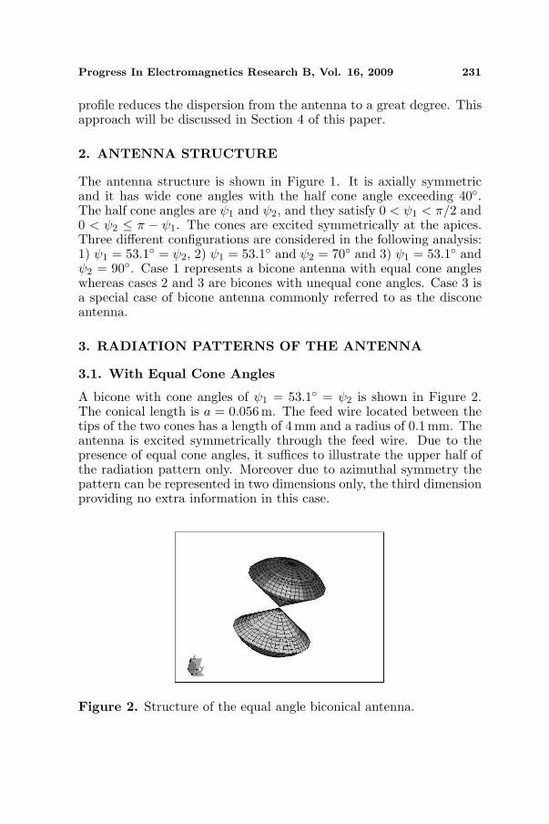
A bicone with cone angles of ψ1 = 53.1◦ = ψ2 is shown in Figure 2.The conical length is a = 0.056m. The feed wire located between thetips of the two cones has a length of 4mm and a radius of 0.1 mm. Theantenna is excited symmetrically through the feed wire. Due to thepresence of equal cone angles, it suffices to illustrate the upper half ofthe radiation pattern only. Moreover due to azimuthal symmetry thepattern can be represented in two dimensions only, the third dimensionproviding no extra information in this case.

Figure 2. Structure of the equal angle biconical antenna.


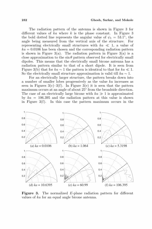
The radiation pattern of the antenna is shown in Figure 3 fordifferent values of ka where k is the phase constant. In Figure 3the bold dotted line represents the angular value of ψ1 = 53.1◦, theangle being measured from the vertical axis of the structure. Forrepresenting electrically small structures with ka ¿ 1, a value ofka = 0.0106 has been chosen and the corresponding radiation patternis shown in Figure 3(a). The radiation pattern in Figure 3(a) is aclose approximation to the sin θ pattern observed for electrically smalldipoles. This means that the electrically small bicone antenna has aradiation pattern similar to that of a short dipole. It is seen fromFigure 3(b) that for ka ∼ 1 the pattern is identical to that for ka ¿ 1.So the electrically small structure approximation is valid till ka ∼ 1.

For an electrically larger structure, the pattern breaks down intoa number of smaller lobes progressively as the value ka increases asseen in Figures 3(c)–3(f). In Figure 3(e) it is seen that the patternmaximum occurs at an angle of about 25◦ from the broadside direction.The case of an electrically large bicone with ka À 1 is approximatedby ka = 106.395 and the radiation pattern at this value is shownin Figure 3(f). In this case the pattern maximum occurs in the

1

0.8

0.6

0.4

0.2

1

0.8

0.6

0.4

0.2

1

0.8

0.6

0.4

0.2

(a) ka = 0.0106 (b) ka = 1.064 (c) ka = 5.3198

(d) ka = 10.6395 (e) ka = 60.99 (f) ka = 106.395

1

0.8

0.6

0.4

0.2

1

0.8

0.6

0.4

0.2

1

0.8

0.6

0.4

0.2

Figure 3. The normalized E-plane radiation pattern for differentvalues of ka for an equal angle bicone antenna.


broadside direction. Moreover, for both Figure 3(e) and Figure 3(f)the radiation pattern lies within 36.9◦ of the broadside direction where(π/2 − ψ1) = 36.9◦ represents the conical angle defined by the biconestructure. These patterns show that for electrically large biconeantennas most of the energy is concentrated in the conical area outlinedby the conical edges and when ka is sufficiently large, the pattern hasa maximum in the broadside direction with very little energy radiatingoutside the above mentioned area. Thus if the directivity requirementsof the communication system under consideration are known, one candesign a biconical antenna to suit the application by determining thecone angles of the antenna. While designing such an antenna, it isimportant to remember that the designed antenna has to be used in afrequency range limited by ka À 1.

30

60

90

0

NUMERICAL

0.5

1

30

60

90

0

0.5

1

30

60

90

0

1

0.8

0.6

0.4

0.2

ANALYTICAL

(a) ka = 0.0106

30

60

90

0

1

0.8

0.6

0.4

0.2

NUMERICAL

ANALYTICAL

NORMALIZED ERROR

(b) ka = 1.064

NUMERICAL

ANALYTICAL

NORMALIZED ERROR

NUMERICAL

ANALYTICAL

NORMALIZED ERROR

NUMERICAL

ANALYTICAL

NORMALIZED ERROR

NUMERICAL

ANALYTICAL

NORMALIZED ERROR

30

60

90

0

1

0.8

0.6

0.4

0.2

30

60

90

0

1

0.8

0.6

0.4

0.2

(c) ka = 5.3198

(d) ka = 10.6395

1.51.5

(e) ka = 60.99 (f) ka = 106.395

Figure 4. Comparison of the normalized E-plane radiation patternsand the error for an equal angle bicone antenna.


3.2. Comparison of the Radiation Patterns Obtained fromAnalytical and Numerical Calculations

The relative radiated field pattern in the E-plane can be calculatedanalytically as follows [4]:

R (θ, ω) =Erad

θ (r, θ, ω)Erad

θ (r, π/2, ω)=

∑∞n=1

in−1(2n+1)2n(n+1)

P 1(cos θ)gn(µ1,µ2)

h(2)n−1(ka)− n

kah(2)n (ka)

∑∞n=1

in−1(2n+1)2n(n+1)

P 1(0)gn(µ1,µ2)

h(2)n−1(ka)− n

kah(2)n (ka)

(1)

Each series in (1) is truncated after (M + 1) terms where M isgiven in the Table 1 of [6]. The analytically calculated radiated field iscompared to the field obtained numerically as described in the previoussection. The comparison shows that as the value of ka increasesthe difference in the two calculations is larger. The normalizederror between the theoretical and numerical results is calculated as‖Rtheo−Rnum‖

‖Rtheo‖ , where Rtheo in the theoretical field and Rnum is thenumerically calculated field and they are shown in Figures 4(a)–4(f).When ka ≤ 10.6395 the fields are identical differing slightly between35◦ and 70◦. But for ka > 10.6395 the difference between thetheoretical and numerical calculations is much more significant dueto the approximations in the theoretical calculation.

3.3. With Unequal Cone Angles

3.3.1. Cone Angles of ψ1 = 53.1◦ and ψ2 = 70◦

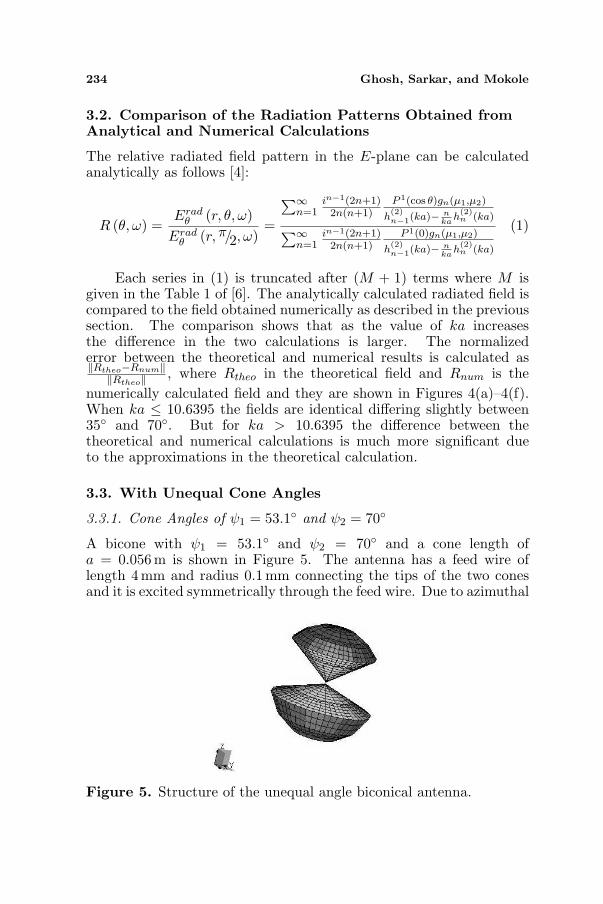
A bicone with ψ1 = 53.1◦ and ψ2 = 70◦ and a cone length ofa = 0.056m is shown in Figure 5. The antenna has a feed wire oflength 4 mm and radius 0.1 mm connecting the tips of the two conesand it is excited symmetrically through the feed wire. Due to azimuthal

Figure 5. Structure of the unequal angle biconical antenna.


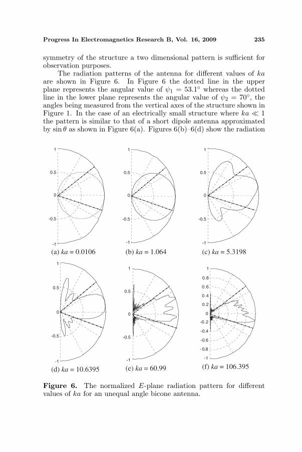
symmetry of the structure a two dimensional pattern is sufficient forobservation purposes.

The radiation patterns of the antenna for different values of kaare shown in Figure 6. In Figure 6 the dotted line in the upperplane represents the angular value of ψ1 = 53.1◦ whereas the dottedline in the lower plane represents the angular value of ψ2 = 70◦, theangles being measured from the vertical axes of the structure shown inFigure 1. In the case of an electrically small structure where ka ¿ 1the pattern is similar to that of a short dipole antenna approximatedby sin θ as shown in Figure 6(a). Figures 6(b)–6(d) show the radiation

0.2

0.4

0.6

0.8

1

0

-0.2

-0.4

- 0.8

-0.6

-1

1

0.5

0

-0.5

-1

1

0.5

0

-0.5

-1

1

0.5

0

-0.5

-1

1

0.5

0

-0.5

-1

1

0.5

0

-0.5

-1

(d) ka = 10.6395 (e) ka = 60.99 (f) ka = 106.395

(a) ka = 0.0106 (b) ka = 1.064 (c) ka = 5.3198

Figure 6. The normalized E-plane radiation pattern for differentvalues of ka for an unequal angle bicone antenna.


patterns of the antenna for three transitional values of ka. The case ofelectrically large bicone where ka À 1 is approximated by ka = 60.99in Figure 6(e) and by ka = 106.395 in Figure 6(f). In Figures 6(e)and 6(f) the patterns break down into a number of small lobes. Forboth Figure 6(e) and Figure 6(f) the radiation pattern lies withinan angular area limited by 36.9◦ above and 20◦ below the broadsidedirection where (π/2 − ψ1) = 36.9◦ and (π/2− ψ2) = 20◦. Thesecalculations verify that for electrically large biconical structures mostof the energy is concentrated in the conical area outlined by the coneangles of the bicone. During the design of a communication or radarsystem, one can determine the angles between which the radiation hasto be limited for the specific application at hand. Then using theangular data obtained, a biconical antenna can be designed to suit theapplication.

3.3.2. Cone Angles of ψ1 = 53.1◦ and ψ2 = 90◦

A bicone with ψ1 = 53.1◦ and ψ2 = 90◦ and a cone length ofa = 0.056m is shown in Figure 7. This is a special case ofunequal cone angles of the spherically-capped bicone antenna as thisantenna is similar to a discone antenna with spherical caps. Like theprevious cases the antenna has a feed wire of length 4 mm and radius0.1mm connecting the tips of the two cones. The antenna is excitedsymmetrically through the feed wire. Due to azimuthal symmetry ofthe structure a two dimensional radiation pattern is shown.

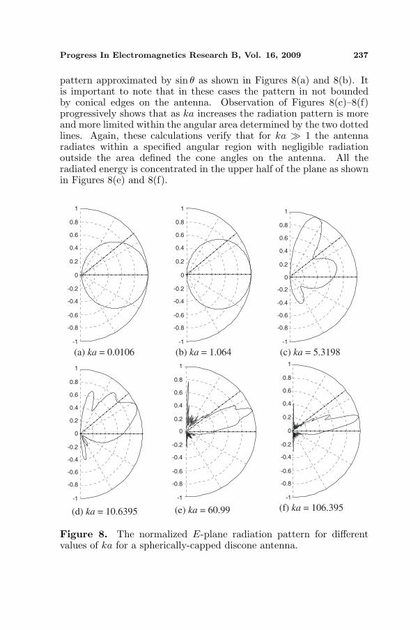
The radiation pattern of the antenna for different values of kais shown in Figure 8. Two dotted lines are drawn in Figure 8, onerepresents the angular value of ψ1 = 53.1◦ and the other representsψ2 = 90◦, the angles being measured from the vertical axis of thestructure shown in Figure 1. In the case of an electrically smallstructure where ka ¿ 1 the pattern is similar to that of a short dipole

Figure 7. Structure of the spherically-capped discone antenna.


pattern approximated by sin θ as shown in Figures 8(a) and 8(b). Itis important to note that in these cases the pattern in not boundedby conical edges on the antenna. Observation of Figures 8(c)–8(f)progressively shows that as ka increases the radiation pattern is moreand more limited within the angular area determined by the two dottedlines. Again, these calculations verify that for ka À 1 the antennaradiates within a specified angular region with negligible radiationoutside the area defined the cone angles on the antenna. All theradiated energy is concentrated in the upper half of the plane as shownin Figures 8(e) and 8(f).

1

0.8

0.6

0.4

0.2

0

-0.2

-0.4

-0.6

-0.8

-1

1

0.8

0.6

0.4

0.2

0

-0.2

-0.4

-0.6

-0.8

-1

1

0.8

0.6

0.4

0.2

0

-0.2

-0.4

-0.6

-0.8

-1

1

0.8

0.6

0.4

0.2

0

-0.2

-0.4

-0.6

-0.8

-1

1

0.8

0.6

0.4

0.2

0

-0.2

-0.4

-0.6

-0.8

-1

1

0.8

0.6

0.4

0.2

0

-0.2

-0.4

-0.6

-0.8

-1

(a) ka = 0.0106 (b) ka = 1.064 (c) ka = 5.3198

(d) ka = 10.6395 (e) ka = 60.99 (f) ka = 106.395

Figure 8. The normalized E-plane radiation pattern for differentvalues of ka for a spherically-capped discone antenna.


4. TRANSIENT RADIATED AND RECEIVED FIELDSOF A BICONE

In Section 3, it is shown that depending on the requirements of thesystem, a biconical antenna can be designed to have a radiation patterndirected in a desired region. This is an important step in efficientsystem design. Additionally, many of the current communication andradar systems call for wideband antennas. Thus it is very usefulto design a bicone antenna which is directive as well as wideband.This section will address the design of ultra-wideband or UWB biconeantennas. Again in the previous section, it is shown that an electricallysmall bicone antenna behaves very similarly to a dipole antenna bothdemonstrating isotropic patterns. But the difference is that the dipoleis a very narrowband antenna whereas the spherically capped biconeantenna has much wider bandwidth. Thus if the communicationsystem warrants an antenna with a dipole-like wideband pattern, thenthe wideband biconical antenna can be used for such applications.Before illustrating the design of a wideband bicone structures, thecommonly used wideband input pulses are investigated.

4.1. Input Pulse

Commonly used baseband pulses are impulses and monocycles. Themonocycle is a doublet formed by the differentiation of the impulse orby the double-differentiation of the step function. As the monocyclehas both positive and negative pulses, it is useful for driving both halvesof the symmetrical biconical antennas. Additionally, the symmetricalnature of the monocycle does not permit the generation of dc currentsduring numerical computation, so the output of an antenna excitedby a monocycle pulse has no dc component. The usefulness of themonocycle pulse is evident from the paper by Ghosh, et al. [8] wherethe monocycle has been successfully used as input to various UWBantennas. In this case, the monocycle pulse is obtained by taking thetime derivative of a short duration Gaussian pulse. The monocyclepulse has the form

~Einc(t) = ~uiE0

σ√

π

d

dt

exp

−

(t− t0 − ~r · ~k

)2

σ2

(2)

where ~ui is the unit vector that defines the polarization of the incomingplane wave, E0 is the amplitude of the incoming wave (chosen to be377V/m), σ controls the width of the pulse, t0 is the delay that is used


to ensure the pulse rises smoothly from 0 at the initial time to its valueat time t, ~r is the position of an arbitrary point in space, and ~k is theunit wave vector defining the direction of arrival of the incident pulse.The frequency spectrum of (2) is given by

E(jω) = ~uiE0jω exp(−σ2ω2

4− jω

(t0 + ~r · ~k

))(3)

where f is the frequency of the signal and ω = 2πf .The duration of the pulse is chosen corresponding to the frequency

range of operation of the antenna. In the case of an electricallysmall bicone antenna, simulation is done between 3MHz and 300 MHz.The input monocycle has a width of 4.5 lm and a time delay of9 lm. Throughout the paper the unit of time is a light meter (lm),a measure of the time required by light to travel 1m. So 1 lm =(speed of light)−1 = 3.3333 × 10−9 s. The input pulse is shown inFigure 9(a). For an electrically large bicone antenna, simulation iscarried out for a wide band of frequencies ranging from 300MHz to26GHz. The input pulse has a width of 0.0437 lm and a time delayof 0.0575 lm. This input pulse is shown in Figure 9(b). The transientfields are normalized for comparison purposes.

4.2. Electrically Small Antenna with Dipole-like RadiationPattern

The transient radiated and received fields of the antenna for the threedifferent cases discussed above are obtained. The cases are: case 1:

0 5 10 15 20 25 30-1

-0.8

-0.6

-0.4

-0.2

0

0.2

0.4

0.6

0.8

1

0 0.05 0.1 0.15 0.2 0.25 0.3 0.35 0.4-1

-0.8

-0.6

-0.4

-0.2

0

0.2

0.4

0.6

0.8

1

INP

UT

VO

LT

AG

E

INP

UT

VO

LT

AG

E

(a) (b)

TIME (in lm) TIME (in lm)

Figure 9. (a) Monocycle input pulse for electrically small antenna.(b) Monocycle input pulse for electrically large antenna.


ψ1 = 53.1◦ = ψ2, case 2: ψ1 = 53.1◦ and ψ2 = 70◦, and case 3:ψ1 = 53.1◦ and ψ2 = 90◦. In each case, the antenna is simulated as aradiator and the radiated field is observed in the broadside direction.Next the antenna is simulated as a receiver for an incident waveapproaching from the broadside direction. The simulation is done overa frequency range of 3 MHz to 300 MHz such that ka < 1.064 and thetransient fields are obtained by the procedure explained in Section 1 ofthis paper. It has been shown in Section 3 that for values of ka < 1.064,the antenna behaves as an electrically small structure. The radiatedfields due to the input pulse of Figure 9(a) for all the three cases areshown in Figure 10(a) and the induced currents on the bicones for anincident wave as in Figure 9(a) are shown in Figure 10(b). Figure 10shows that the transient responses of all the three antennas are exactlysame, signifying that the change in cone angle has no effect on thetransient response of the antenna if the antenna is operated in therange of ka ¿ 1.

As the antenna has a pattern similar to that of a short dipole asshown in Figures 3(a), 6(a) and 8(a), the radiated field of the biconeshould be similar to the radiated field of a short dipole. In the case ofan electrically small dipole, the far field is proportional to the secondtemporal derivative of the transient current on the structure whereasthe received open circuit voltage is approximately the derivative of theincident field [8, 9]. This statement is verified by Figure 10(a) where theradiated field is the second derivative of the monocycle input voltageshown in Figure 9(a) and by Figure 10(b) where the received field isthe derivative of the monocycle incident wave of Figure 9(a). As theradiated and received fields do not show any ringing, this antenna issuitable for ultra-wideband application for ka ¿ 1.

0 5 10 15 20 25 30-1

-0.8

-0.6

-0.4

-0.2

0

0.2

0.4

0.6

0.8

1ψ ψ=53.1=1 2ψ ψ=53.1,1 2=70ψ ψ=53.1,1 2=90

ψ ψ=53.1=1 2ψ ψ=53.1,1 2=70ψ ψ=53.1,1 2=90

1

0.5

0

-0.50 5 10 15 20 25 30

CU

RR

EN

T

E-F

IELD

TIME (in lm)TIME (in lm)

(a) (b)

Figure 10. Radiated field for an electrically small antenna.


4.3. Electrically Large Antenna for Angle-specificApplications

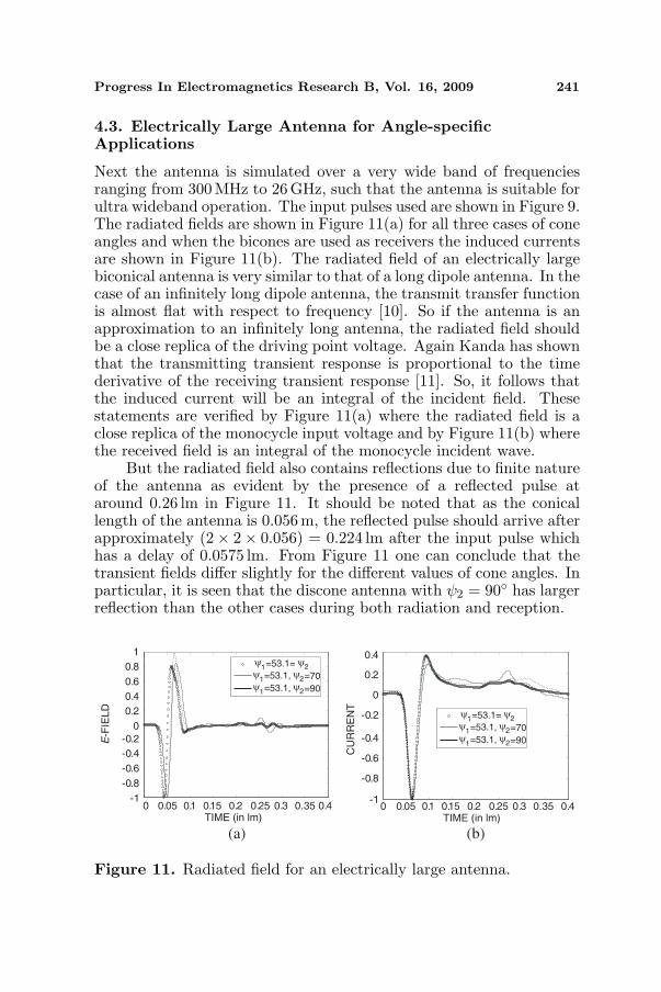
Next the antenna is simulated over a very wide band of frequenciesranging from 300 MHz to 26 GHz, such that the antenna is suitable forultra wideband operation. The input pulses used are shown in Figure 9.The radiated fields are shown in Figure 11(a) for all three cases of coneangles and when the bicones are used as receivers the induced currentsare shown in Figure 11(b). The radiated field of an electrically largebiconical antenna is very similar to that of a long dipole antenna. In thecase of an infinitely long dipole antenna, the transmit transfer functionis almost flat with respect to frequency [10]. So if the antenna is anapproximation to an infinitely long antenna, the radiated field shouldbe a close replica of the driving point voltage. Again Kanda has shownthat the transmitting transient response is proportional to the timederivative of the receiving transient response [11]. So, it follows thatthe induced current will be an integral of the incident field. Thesestatements are verified by Figure 11(a) where the radiated field is aclose replica of the monocycle input voltage and by Figure 11(b) wherethe received field is an integral of the monocycle incident wave.

But the radiated field also contains reflections due to finite natureof the antenna as evident by the presence of a reflected pulse ataround 0.26 lm in Figure 11. It should be noted that as the conicallength of the antenna is 0.056m, the reflected pulse should arrive afterapproximately (2× 2× 0.056) = 0.224 lm after the input pulse whichhas a delay of 0.0575 lm. From Figure 11 one can conclude that thetransient fields differ slightly for the different values of cone angles. Inparticular, it is seen that the discone antenna with ψ2 = 90◦ has largerreflection than the other cases during both radiation and reception.

ψ ψ=53.1=1 2ψ ψ=53.1,1 2=70ψ ψ=53.1,1 2=90

ψ ψ=53.1=1 2ψ ψ=53.1,1 2=70ψ ψ=53.1,1 2=90

-1

-0.8

-0.6

-0.4

-0.2

0

0.2

0.4

0.6

0.8

1

E-F

IELD

0 0.05 0.1 0.15 0.2 0.25 0.3 0.35 0.4TIME (in lm)

-1

-0.8

-0.6

-0.4

-0.2

0

0.2

0.4

CU

RR

EN

T

0 0.05 0.1 0.15 0.2 0.25 0.3 0.35 0.4TIME (in lm)

(a) (b)

Figure 11. Radiated field for an electrically large antenna.


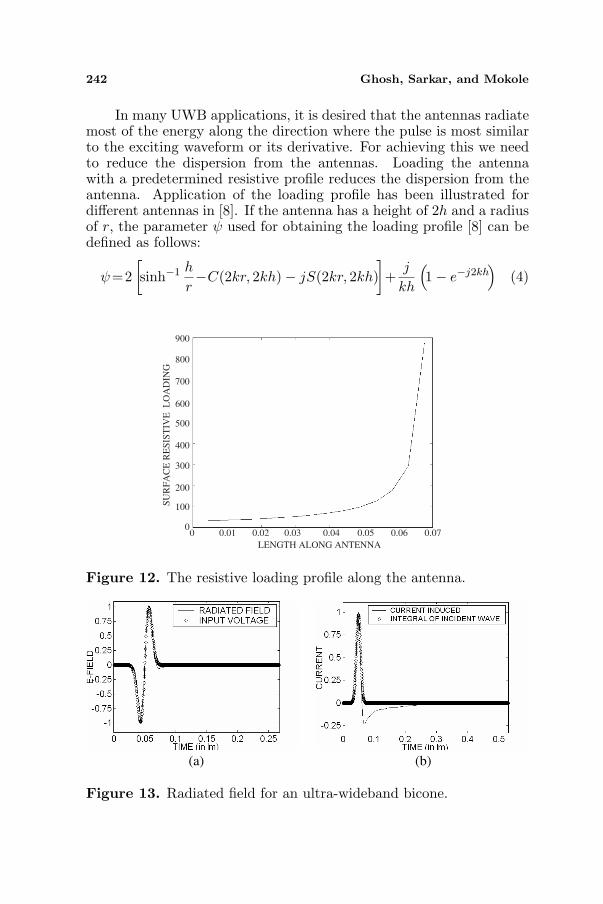
In many UWB applications, it is desired that the antennas radiatemost of the energy along the direction where the pulse is most similarto the exciting waveform or its derivative. For achieving this we needto reduce the dispersion from the antennas. Loading the antennawith a predetermined resistive profile reduces the dispersion from theantenna. Application of the loading profile has been illustrated fordifferent antennas in [8]. If the antenna has a height of 2h and a radiusof r, the parameter ψ used for obtaining the loading profile [8] can bedefined as follows:

ψ=2[sinh−1 h

r−C(2kr, 2kh)− jS(2kr, 2kh)

]+

j

kh

(1− e−j2kh

)(4)

0 0.01 0.02 0.03 0.04 0.05 0.06 0.07

LENGTH ALONG ANTENNA

SU

RF

AC

E R

ES

IST

IVE

L

OA

DIN

G

900

800

700

600

500

400

300

200

100

0

Figure 12. The resistive loading profile along the antenna.

(a) (b)

Figure 13. Radiated field for an ultra-wideband bicone.


where C(a, x) and S(a, x) are the generalized cosine and sine integrals:

C(a, x) =

x∫

0

1− cosW

Wdu S(a, x) =

x∫

0

sinW

Wdu (5)

withW = (u2 + a2)1/2 (6)

So the continuously varying resistive profile can be defined as

zi(z) = ri(z)− j/ω ci(z) =ζ0ψ

2π

1h− |z| =

60ψh− |z| (7)

In this formula the frequency dependence appears only in the formof a logarithm for small values of kh, so the antenna shows very broadfrequency characteristics. The reactive part of the impedance is verysmall compared to the resistive part, so we do not need to implementthe capacitive profile in this case. The value of ψ at the frequencyfor which the bicone is a half-wavelength long is calculated and theeffective radius for the load calculation in (4) is taken to be one-hundredth of the length of the bicone to meet the specification fora thin antenna. The antenna has been divided into lateral regionsalong its length and distributed loading is applied on each region bycalculating the resistivity at the midpoint of that region. If the numberof sections is sufficiently large, then the step-functional variation of theresistance will bear a close resemblance to the continuously varyingresistive profile (Figure 12). The radiated field for this non-reflectingantenna nearly coincides with the input voltage (Figure 13(a)), whichverifies that the reflectionless bicone behaves like an infinitely longdipole. If the antenna is used as a receiver, the received current at thefeed point of the antenna deviates slightly from the integral of the inputvoltage (Figure 13(b)). This discrepancy is due to the absence of anydc current on the structure. This methodology illustrates the designof a angle-specific ultra-wideband antenna using bicone structures.

5. CONCLUSION

The spherically capped bicone antenna has been extensively studiedin this paper. The antenna is considered with equal cone angles andwith unequal cone angles. An investigation of the radiation patternof the antenna shows that for ka ¿ 1 the radiation pattern can beapproximated by sin θ whereas for ka À 1 the pattern lies within anangular area determined by the cone angles of the antenna. As an


example we can limit the radiation energy in the upper half of theE-plane within an angular region of 36.9◦ by choosing ψ1 = 53.1◦ andψ2 = 90◦.

The transient response of the antenna has also been investigatedfor both radiation and reception for different sets of cone angles.Observation of the wave shapes from the antennas give importantinformation about their transmitting and receiving properties andrelationships can be obtained between the input and output waveshapes. Moreover it is observed that when ka ¿ 1 the transient fieldsand currents are not affected by the change in the cone angles. But forka À 1 there are reflections due to the finite nature of the antenna andthese reflections change slightly with changes in the cone angle values.

The bicone antenna can be designed to have ultra-widebandbehavior by using a spherical cap and by applying resistive loading onthe structure. This antenna radiates most of the energy in the directionwhere the pulse is most similar to the exciting waveform. This propertyis very critical in the operation of ultra-wideband structures. Thuswhether the need is for a wideband antenna with dipole-like isotropicpatterns or for an ultra-wideband antenna with radiation constrainedwithin a particular angular area, one can design it with a sphericallycapped bicone antenna as illustrated in this paper.

REFERENCES

1. Schelkunoff, S. A., Electromagnetic Waves, Vol. 9, Van Nostrand,New York, 1943.

2. Smith, P. D. P., “The conical dipole of wide-angle,” Journal ofApplied Physics, Vol. 19, 11–23, 1948.

3. Papas, C. H. and R. W. P. King, “Input impedance of wide-angleconical antennas fed by a coaxial line,” Proceedings IRE, Vol. 37,1269–1271, 1949.

4. Papas, C. H. and R. W. P. King, “Radiations from wide-angleconical antenna fed by a coaxial line,” Proceeding IRE, Vol. 39,49–51, 1951.

5. Sandler, S. S. and R. P. W. King, “Compact conical antennafor wide-band coverage,” IEEE Transactions on Antenna andPropagation, Vol. 42, 436–439, Mar. 1994.

6. Samaddar, S. N. and E. L. Mokole, “Biconical antenna withunequal cone angles,” IEEE Transactions on Antenna andPropagation, Vol. 46, No. 2, 181–193, 1998.

7. Kolundzija, B. M., J. S. Ognjanovic, and T. K. Sarkar, WIPL-D:


Software for Electromagnetic Analysis of Composite Wire, Plateand Dielectric Structures, Artech House, 1995.

8. Ghosh, D., A. De, M. C. Taylor, T. K. Sarkar, M. C. Wicks,and E. Mokole, “Transmission and reception by ultra wideband(UWB) antennas,” IEEE Antenna and Propagation Magazine,Vol. 48, No. 5, 66–99, Oct. 2006.

9. Sarkar, T. K., M. C. Wicks, M. Salazar-Palma, and R. J. Bonneau,Smart Antennas, Wiley-IEEE Press, Apr. 22, 2003.

10. Harrison, C. W. and R. W. P. King, “On the transient response ofan infinite cylindrical antenna,” IEEE Transactions on Antennaand Propagation, 301–302, 1967.

11. Kanda, M., “Time domain sensors and radiators,” Time DomainMeasurements in Electromagnetics, E. K. Miller (ed.), Vol. 5, VanNostrand Reinhold, New York, 1986.

12. Chisholm, W. A. and W. Janischewskyj, “Lightning surgeresponse of ground electrodes,” IEEE Trans. on Power Delivery,Vol. 4, No. 2, 1329–1337, Apr. 1989.

13. Baba, Y. and V. A. Rakov, “On the interpretation ofground reflections observed in small-scale experiments simulatinglightning strikes to towers,” IEEE Trans. on EMC, Vol. 47, No. 3,533–542, Aug. 2005.

design of a wide-angle biconical antenna for wideband communications … · progress in...

Documents