design of a replacement german main battle tank in...

Design of a Replacement German Main Battle Tank in 1941

Andrew Alan Rader December 17, 2007

ESD 1.71 Final Project

ESD 71 Final Application Portfolio, 2007 Andrew Rader

2 of 23

Table of Contents 1. Introduction ...............................................................................................................................4 2. System Description....................................................................................................................4 2.1 Choices available ............................................................................................................. 5 2.2 Variables considered in this study................................................................................... 6 2.3 Variables outside the scope of this study........................................................................ 6 2.4 Flexibility in the design .................................................................................................... 7 2.5 Armor Thickness .............................................................................................................. 7 2.6 Armor composition.......................................................................................................... 8 2.7 Output (Benefit) .............................................................................................................. 9 2.8 Input (Cost) .................................................................................................................... 10

3. Decision Analysis .....................................................................................................................11 3.1 Maximum and minimum designs .................................................................................. 12 3.2 Flexible designs.............................................................................................................. 12 3.3 Decision analysis first stage........................................................................................... 14 3.4 Decision analysis second stage...................................................................................... 15

4. Lattice Analysis........................................................................................................................17 4.1 Lattice parameters......................................................................................................... 17 4.2 Outcomes and probabilities .......................................................................................... 17 4.3 Option analysis .............................................................................................................. 18 4.4 Dynamic programming .................................................................................................. 20

5. Discussion and conclusions ...................................................................................................21 Acronyms, Symbols, and Definitions AP: Armor piercing; ability to penetrate steel plate armor AF: Armor fraction; fraction of combat encounters vs. armored forces AT: Armor thickness; weighted average of Soviet armor thicknesses HE: High explosive; explosive capability of shell – proportional to shell weight Δt: Time period; in this case 1 year v: Mean rate of increase of AT σ: Standard deviation of AT increase u: “Up” value for lattice analysis d: “Down” value for lattice analysis p: Probability of “Up” (vs. “Down”) for lattice analysis -The word “panzer”, meaning “armor” in German is short for “panzerkampfwagon”, or “armored fighting vehicle”, and will be used interchangeably with the word “tank” in this report. -The main measurement of gun size is caliber, which is the diameter of the shell fired. For example, a 75 mm gun fires a shell 75 mm in diameter and about a foot and a half in length. The designation for the guns described often has a length rating which affects armor piercing capability at a cost of weight of the gun and supporting turret and chassis. For example, a 75 mm L/43 gun is 75 mm in diameter and 75 mm x 43 = 3225 mm (3.23 m) in length. Generally, a longer gun results in a faster muzzle velocity, increasing armor penetration, at the cost of weight and ease of manufacture.


3 of 23

Abstract This report examines the decisions facing German panzer designers in 1941 when it suddenly became apparent that their armored vehicles were inadequately armed to deal with Soviet forces. A new flexible panzer design is proposed, and decision and lattice analyses are conducted with 1 year periods to determine the ideal time to up-gun the vehicle with contemporary German anti-tank weapons to optimally respond to increasing Soviet armor strength. The analysis uses historical data to examine armor penetration and high explosive capabilities of the guns, typical combat ranges, fixed and flexible panzer weights, as well as Soviet force composition and armor strength. The decision and lattice analyses yield similar – and remarkably historic – results, and favor the flexible design with a 75 mm gun initially, with the ability to upgrade to an 88 mm gun in the 2-4 year time frame to keep pace with Soviet armor.


4 of 23

1. Introduction Germany unleashed Blitzkrieg on an unsuspecting world in 1939, and, until mid-1942, enjoyed a tremendous advantage in armored warfare. Contrary to popular conceptions, and with few exceptions, this was not due to any particular technical superiority of their vehicles, but rather to fire support, training, tactics, and the flexibility of their organizational structure. For example, all ranks were trained to be able to perform not only their jobs, but the jobs of a rank at least one level higher1. Other factors played major roles in their superiority: at the start of the war, every German tank carried a radio; it was not until 1943 that this was true of their opponents2. Even with these advantages, during the invasion of the Soviet Union in 1941, the superiority of their panzer divisions began to waver as German forces encountered vehicles that were far more heavily armed, armored, and better suited to Russian fighting conditions. German soldiers found to their horror that they had very few weapons (the 88mm dual purpose anti-aircraft gun being the only notable exception) capable of penetrating the armor of most of the latest Soviet tank designs, such as the T-34 and KV series. The search for a replacement for the Panzers III and IV models (originally conceived as the main battle tanks) became a national priority that would eventually result in the superb Panzer V (Panther) and Panzer VI (Tiger) models introduced in 1943 and late 1942, respectively – among the best tank designs of the war. The search for these main battle tank replacements was dependent on many factors: performance requirements, available materials, operational conditions, design, prototyping, and production-line economics, technological change, and, most importantly, the opposition to be faced then and in the future (enemy tanks, aircraft, artillery, and anti-tank weapons). All of these factors had to be considered very quickly, as it was critical to push a replacement vehicle into service as quickly as possible. Armor and gun designers have always faced an escalating arms race, and this recursive effect means that no design is final. A larger gun necessitates thicker armor for protection, which results in the need for a more powerful gun, and so on. Naval engineers have been confronted with this reality since cannons were first mounted on ships. The main problem facing the panzer forces in 1941 was that their current vehicles were simply not equipped with a gun sufficiently powerful to penetrate the armor of new Soviet tanks (and even some British models such as the Matilda II) at any reasonable range. The Panzer III was equipped with a 50 mm gun, and its chassis was not large enough to mount a heavier one. The Panzer IV was equipped with a 75 mm howitzer – large enough, but with too low a muzzle velocity for armor penetration. The primary requirement was thus mounting a larger and more powerful gun. Many options were available, and each introduced a tradeoff between armor piecing and high explosive effectiveness, range, shell size, accuracy, and manufacturability.

2. System Description The objective of this application portfolio will be to examine the choices available to German tank designers in late 1941 to upgrade their panzer forces to meet present and future Soviet threats. The vehicles then in service were not sufficient to counter emerging Soviet vehicles, largely because they were not designed to be able to mount a sufficiently powerful main gun. Thus, a redesign of a new vehicle was necessary, but it was not know exactly what type of gun should be used, nor how best to up-gun or replace the vehicle to counter unforeseen or future enemy armor developments. Many


5 of 23

factors would have been considered the designers at the time, but most are beyond the scope of this study; the objective here is to focus on gun selection, and in particular, how flexibility can be used to up-gun as necessary.

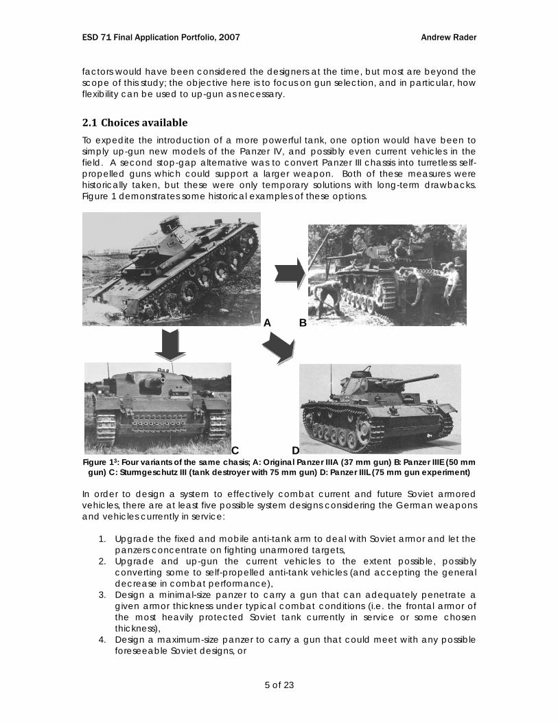
2.1 Choices available To expedite the introduction of a more powerful tank, one option would have been to simply up-gun new models of the Panzer IV, and possibly even current vehicles in the field. A second stop-gap alternative was to convert Panzer III chassis into turretless self-propelled guns which could support a larger weapon. Both of these measures were historically taken, but these were only temporary solutions with long-term drawbacks. Figure 1 demonstrates some historical examples of these options.

A B

C D Figure 13: Four variants of the same chasis; A: Original Panzer IIIA (37 mm gun) B: Panzer IIIE (50 mm

gun) C: Sturmgeschutz III (tank destroyer with 75 mm gun) D: Panzer IIIL (75 mm gun experiment) In order to design a system to effectively combat current and future Soviet armored vehicles, there are at least five possible system designs considering the German weapons and vehicles currently in service:

1. Upgrade the fixed and mobile anti-tank arm to deal with Soviet armor and let the panzers concentrate on fighting unarmored targets,

2. Upgrade and up-gun the current vehicles to the extent possible, possibly converting some to self-propelled anti-tank vehicles (and accepting the general decrease in combat performance),

3. Design a minimal-size panzer to carry a gun that can adequately penetrate a given armor thickness under typical combat conditions (i.e. the frontal armor of the most heavily protected Soviet tank currently in service or some chosen thickness),

4. Design a maximum-size panzer to carry a gun that could meet with any possible foreseeable Soviet designs, or


6 of 23

5. Incorporate flexibility by designing a vehicle larger than necessary to equip it with a gun type that is available now and adequate for the present, but that can be up-gunned sufficiently as Soviet armor thickness increases.

Note that the first two choices involve no new vehicle design, but rather use alternative methods to attempt to deal with the problem. We will thus focus on the last three possibilities. Also, it is likely that the best possible outcome would be to apply one or more of these options in some fashion – we will ignore this for now and focus and finding the best single option.

2.2 Variables considered in this study For simplicity, most of the variables relevant to designing an armored vehicle will be excluded from this study. Only the primary two characteristics will be considered: gun type (and its resulting benefit), and vehicle weight (cost).

2.3 Variables outside the scope of this study Variables such as operational conditions and economic factors are outside the scope of this study, however, they were critical at the time, and so a brief discussion is warranted. Operational conditions The new tanks would be expected to fight in a wide-range of operational conditions, from the freezing winters of Northern Russia to the sweltering deserts of Lybia and Egypt. They would need to operate in areas with little to no infrastructure, poor or no roads (requiring wider tracks and weight minimization), rubble-strewn streets, and in knee-deep mud. They would need to cross rivers with bridges that could not adequately support their size or weight all over Europe. Early panzer variants –unlike their Soviet or Western allied counterparts- were designed to use Petrol (gasoline) so that they could refuel at gas stations along the way. It would be far from certain that these opportunities would be forthcoming later in the war. Economic factors Ultimately, this project, like any other, was subject to a myriad of economic factors. One of the main considerations was whether it would be better to produce many more vehicles of a simpler, cheaper, and easier to mass-produce design (as both the Soviets and Western Allies opted), or produce fewer vehicles of a more complex and powerful one (as the Germans eventually opted for). A more powerful panzer would be harder to field in large numbers, but might have an advantage in battle. The questions of economies of scale and production line economics would have a huge impact on the performance of armies in the field. Availability and cost of materials was another important factor. German resources were stretched and the Allies were doing everything possible to prevent neutral countries from trading valuable or rare materials. For example, a tremendous amount of diplomatic pressure was placed on Portugal, one of the main European sources of Tungsten (critical in armor-piercing shell production), to prevent it from exporting to Germany4. Imports of nickel from Turkey, Iron ore from Sweden, and foreign oil were also under diplomatic attack, and all were in short supply. Dislocation of production due to the intensifying Allied bombing campaign was also a consideration. Organizing production into large concentrated facilities would carry the


7 of 23

risk of making it an easier target for Allied raids. Ideally, the design should be easy to produce at small distributed centers. Other factors Other performance considerations outside the scope of this study include armor slope and thickness, operation range, ammunition capacity, minimization of target profile, crew size and space, and radio.

2.4 Flexibility in the design Flexibility of the design can be introduced by designing a chasis larger than strictly necessary so that the gun can be upgraded as the need arises. This comes at the cost of extra chasis weight.

2.5 Armor Thickness Since the current problem is the inability to adequately deal with Soviet armor, we need to examine the thickness of enemy armor protection. The thickness of armor given to vehicle areas (front, side, turret, etc) varies with combat opportunities (you are more likely to get a shot at the front where it is more heavily protected)5, so we can base our first component of armor thickness (AT) on a weighted average of the mean armor given to vehicles in the front, side, and turret:

AT = v1(tfront + tturret + tsides)/3 + v2(tfront + tturret + tsides)/3 + …,

Where vn is a weight proportional to the number of the nth vehicle type in service.

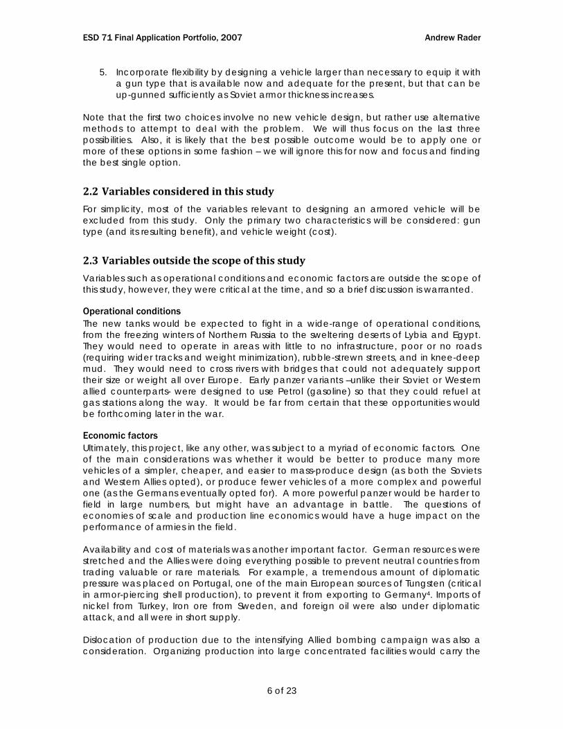
Figure 2 shows mean armor thicknesses for common historical Soviet Tanks, and Table 1 shows the number of vehicles in service in 1941. Some examples of these vehicles are shown in Figure 3.

Figure 2: Soviet armor thickness by vehicle type4

Table 1: Soviet vehicles in service in 19414, 6

Vehicle Year introduced Number of vehicles Older types (BT-5, BT-

7, T-26, etc.) <1939 4000

T-34 1939 1000 KV-1 1941 500 IS-2 1944 0


8 of 23

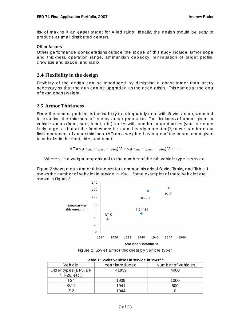
For 1941, this gives us an armor thickness of:

(4000 x 36.7 mm + 1000 x 53 mm + 500 x 116.7 mm)/6500 = 46.9 mm

Figure 3: The opposition – contemporary Soviet designs: BT-5 (top left), T-34 (top right), KV-1 (bottom

left), and IS-2 (bottom right)

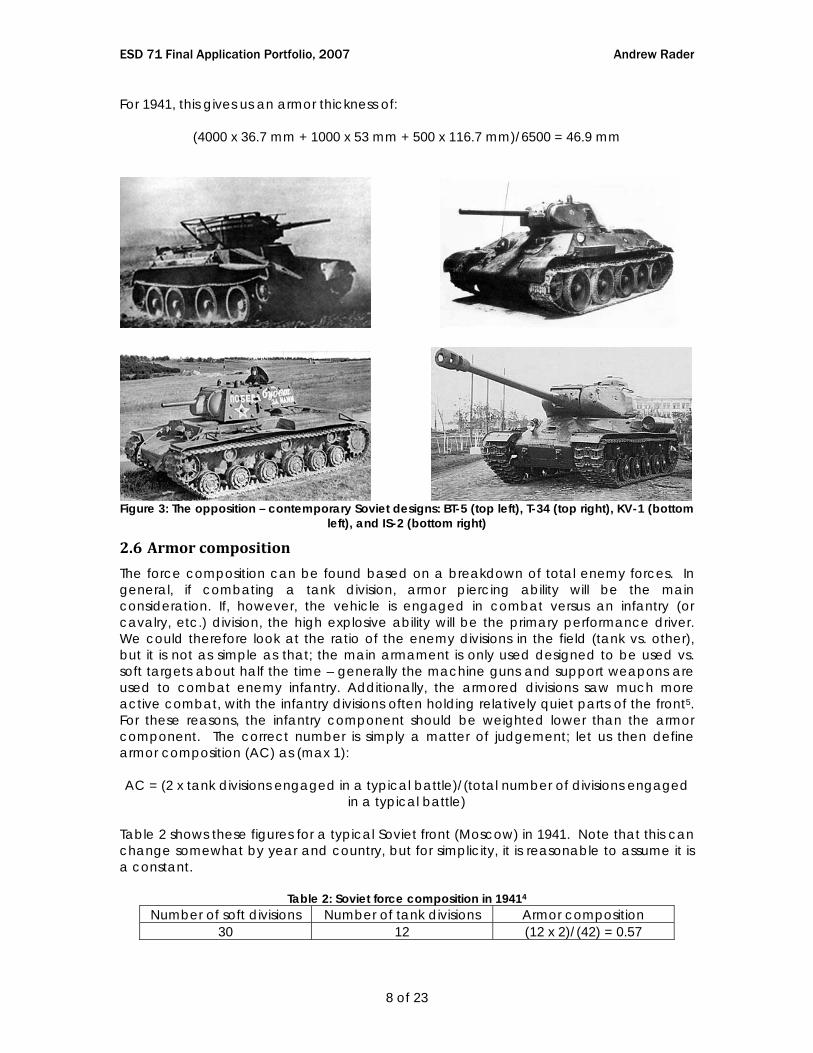
2.6 Armor composition The force composition can be found based on a breakdown of total enemy forces. In general, if combating a tank division, armor piercing ability will be the main consideration. If, however, the vehicle is engaged in combat versus an infantry (or cavalry, etc.) division, the high explosive ability will be the primary performance driver. We could therefore look at the ratio of the enemy divisions in the field (tank vs. other), but it is not as simple as that; the main armament is only used designed to be used vs. soft targets about half the time – generally the machine guns and support weapons are used to combat enemy infantry. Additionally, the armored divisions saw much more active combat, with the infantry divisions often holding relatively quiet parts of the front5. For these reasons, the infantry component should be weighted lower than the armor component. The correct number is simply a matter of judgement; let us then define armor composition (AC) as (max 1): AC = (2 x tank divisions engaged in a typical battle)/(total number of divisions engaged

in a typical battle) Table 2 shows these figures for a typical Soviet front (Moscow) in 1941. Note that this can change somewhat by year and country, but for simplicity, it is reasonable to assume it is a constant.

Table 2: Soviet force composition in 19414 Number of soft divisions Number of tank divisions Armor composition

30 12 (12 x 2)/(42) = 0.57


9 of 23

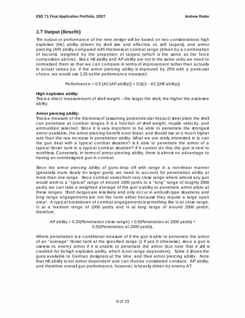
2.7 Output (Benefit) The output or performance of the new design will be based on two considerations: high explosive (He) ability (driven by shell size and effective vs. soft targets), and armor piercing (AP) ability compared with thickness at combat range (driven by a combination of factors), weighted by the proportion of targets (which is the same as the force composition above). Since HE ability and AP ability are not in the same units, we need to normalized them so that we can compare in terms of improvement rather than actually in actual values (i.e. if the armor piercing ability is improved by 25% with a particular choice, we would use 1.25 as the performance measure).

Performance = 0.5 [AC(AP ability)] + 0.5[(1 - AC)(HE ability)] High explosive ability: This is a direct measurement of shell weight – the larger the shell, the higher the explosive ability. Armor piercing ability: This is a measure of the thickness of (assuming perpendicular impact) steel plate the shell can penetrate at combat ranges. It is a function of shell weight, muzzle velocity, and ammunition selected. Since it is very important to be able to penetrate the strongest armor available, the armor piercing benefit is not linear, and should rise at a much higher rate than the raw increase in penetration ability. What we are really interested in is: can the gun deal with a typical combat situation? Is it able to penetrate the armor of a typical Soviet tank in a typical combat situation? If it cannot do this, the gun is next to worthless. Conversely, in terms of armor piercing ability, there is almost no advantage to having an overdesigned gun in combat. Since the armor piercing ability of guns drop off with range in a non-linear manner (generally more slowly for larger guns), we need to account for penetration ability at more than one range. Since combat varies from very close range where almost any gun would work to a “typical” range of around 1000 yards, to a “long” range of roughly 2000 yards, we can take a weighted average of the gun’s ability to penetrate armor plate at these ranges. Short ranges are less likely and only occur in ambush-type situations, and long range engagements are not the norm either because they require a large open area2. A typical breakdown of combat engagements is something like ¼ at close range, ½ at a medium range of 1000 yards, and ¼ at long range of around 2000 yards1; therefore:

AP ability = 0.25(Penetration close range) + 0.5(Penetration at 1000 yards) + 0.25(Penetration at 2000 yards),

Where penetration is a conditional measure of if the gun is able to penetrate the armor of an “average” Soviet tank at the specified range (1 if yes, 0 otherwise), since a gun is useless vs. enemy armor if it is unable to penetrate the armor (but note that it still is credited for its high explosive ability, which is not range dependent). Table 3 shows the guns available to German designers at the time, and their armor piercing ability. Note that HE ability is not armor dependent and can thus be considered constant. AP ability, and therefore overall gun performance, however, is heavily driven by enemy AT.


10 of 23

Table 3: German gun types available or projected in 19414

Gun Shell weight

(kg) Normalized HE

ability Penetration at close range

Penetration at 1000 yrds (mm)

Penetration at 2000 yrds (mm)

50 mm L/43 4 0.14 all 50 30

128mm L/55 28 1 all 180 140

75 mm L/43 6 0.2 all 80 60

75 mm L/48 6 0.2 all 95 60

88 mm L/56 10.2 0.36 all 130 100

88 mm L/71 10.2 0.36 all 150 110

For example, for an enemy AT of 46.9 mm (in 1941), the AP ability of the 50 mm L/43 is:

AP ability of 50 mm L/43 = 0.25 x 1 + 0.5 x 1 + 0.25 x 0 = 0.75 Since this varies between 0 and 1, it is already normalized relative to the ideal condition. Then, applying the performance metric to the gun, we get:

Performance = 0.5[0.57(0.75) + 0.43(0.14)] = 0.25

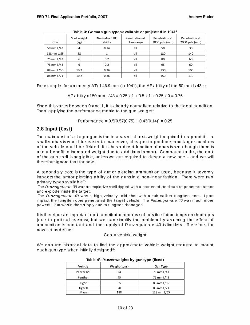
2.8 Input (Cost) The main cost of a larger gun is the increased chassis weight required to support it – a smaller chassis would be easier to maneuver, cheaper to produce, and larger numbers of the vehicle could be fielded. It is thus a direct function of chassis size (though there is also a benefit to increased weight due to additional armor). Compared to this, the cost of the gun itself is negligible, unless we are required to design a new one – and we will therefore ignore that for now. A secondary cost is the type of armor piercing ammunition used, because it severely impacts the armor piercing ability of the guns in a non-linear fashion. There were two primary types available7: -The Panzergranate 39 was an explosive shell tipped with a hardened steel cap to penetrate armor and explode inside the target. -The Panzergranate 40 was a high velocity solid shot with a sub-caliber tungsten core. Upon impact the tungsten core penetrated the target vehicle. The Panzergranate 40 was much more powerful, but was in short supply due to tungsten shortages. It is therefore an important cost contributor because of possible future tungsten shortages (due to political reasons), but we can simplify the problem by assuming the effect of ammunition is constant and the supply of Panzergranate 40 is limitless. Therefore, for now, let us define:

Cost = vehicle weight

We can use historical data to find the approximate vehicle weight required to mount each gun type when initially designed8:

Table 48: Panzer weights by gun type (fixed)

Vehicle Weight (tons) Gun Type

Panzer IVF 24 75 mm L/43

Panther 45 75 mm L/48

Tiger 55 88 mm L/56

Tiger II 70 88 mm L/71 Maus 188 128 mm L/55


11 of 23

For upgrading existing models to larger gun types, there is generally far less of a weight increase (since extra armor is not necessarily needed and more can be added later as necessary). Two salient examples were the up-gunning of the Pz III and Pz IVs, but both of these were up-gunned to similar guns in terms of caliber – in our case similar to going from the 75 mm L/43 to the 75 mm L/482. Both of these models were designed with consideration for the ability to up-grade, and this added something like 25% to the initial weight:

Table 54: Flexibility cost: historical increased weight by up-gunning Vehicle Weight (tons) Weight increase factor

Panzer IIIA 19

Panzer IIIJ 24

1.26

Panzer IVA 20

Panzer IVH 25

1.25

If we wanted to up-gun the caliber of the gun (from 75 mm to 88 mm for example), based on similar historical situations4, we would incur a higher weight penalty of roughly 50%.

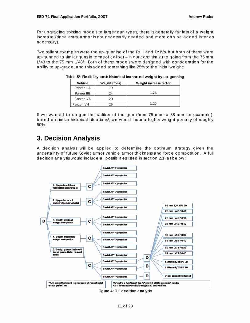
3. Decision Analysis A decision analysis will be applied to determine the optimum strategy given the uncertainty of future Soviet armor vehicle armor thickness and force composition. A full decision analysis would include all possibilities listed in section 2.1, as below:

Figure 4: Full decision analysis


12 of 23

In this project, we will limit our decision analysis to three cases: a minimum weight new panzer, adequate to handle current Soviet threats, a maximum weight panzer able to handle anything foreseeable, and a flexible design that is adequate to meet current threats, and is upgradable to meet future threats, though at an increased initial cost of extra weight. First, we need to define the maximum and minimum design levels.

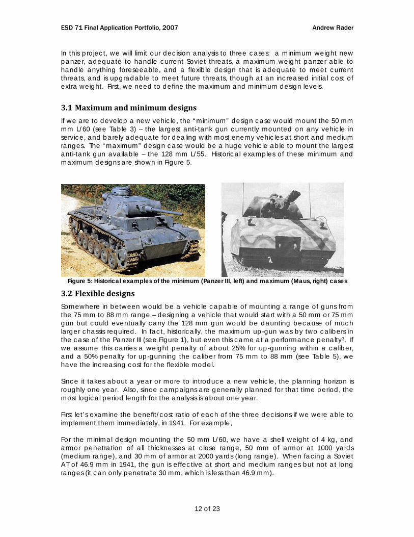
3.1 Maximum and minimum designs If we are to develop a new vehicle, the “minimum” design case would mount the 50 mm mm L/60 (see Table 3) – the largest anti-tank gun currently mounted on any vehicle in service, and barely adequate for dealing with most enemy vehicles at short and medium ranges. The “maximum” design case would be a huge vehicle able to mount the largest anti-tank gun available – the 128 mm L/55. Historical examples of these minimum and maximum designs are shown in Figure 5.

Figure 5: Historical examples of the minimum (Panzer III, left) and maximum (Maus, right) cases

3.2 Flexible designs Somewhere in between would be a vehicle capable of mounting a range of guns from the 75 mm to 88 mm range – designing a vehicle that would start with a 50 mm or 75 mm gun but could eventually carry the 128 mm gun would be daunting because of much larger chassis required. In fact, historically, the maximum up-gun was by two calibers in the case of the Panzer III (see Figure 1), but even this came at a performance penalty3. If we assume this carries a weight penalty of about 25% for up-gunning within a caliber, and a 50% penalty for up-gunning the caliber from 75 mm to 88 mm (see Table 5), we have the increasing cost for the flexible model. Since it takes about a year or more to introduce a new vehicle, the planning horizon is roughly one year. Also, since campaigns are generally planned for that time period, the most logical period length for the analysis is about one year. First let’s examine the benefit/cost ratio of each of the three decisions if we were able to implement them immediately, in 1941. For example, For the minimal design mounting the 50 mm L/60, we have a shell weight of 4 kg, and armor penetration of all thicknesses at close range, 50 mm of armor at 1000 yards (medium range), and 30 mm of armor at 2000 yards (long range). When facing a Soviet AT of 46.9 mm in 1941, the gun is effective at short and medium ranges but not at long ranges (it can only penetrate 30 mm, which is less than 46.9 mm).


13 of 23

Based on the rating system for combat range probabilities, this gives:

AP ability = 0.25 x 1 + 0.5 x 1 + 0.25 x 0 = 0.75 For the other two guns, their AP rating is 1 because they have no trouble penetrating 46.9 mm of armor at any range. The relative AP ranking of the guns is thus 1, 1.33, and 1.33 for the minimal, maximal, and 75 mm flexible designs, respectively. For HE ability, this is a direct function of shell mass, and we get rankings of 1, 7, and 1.5, for the minimal (50 mm; 4 kg), maximal (128 mm; 28 kg), and 75 mm flexible designs (75 mm; 6 kg), respectively. Using the armor composition (AC) based on force composition for 1941 (0.57), we get a normalized gun performance for the minimal 50 mm L/60 of:

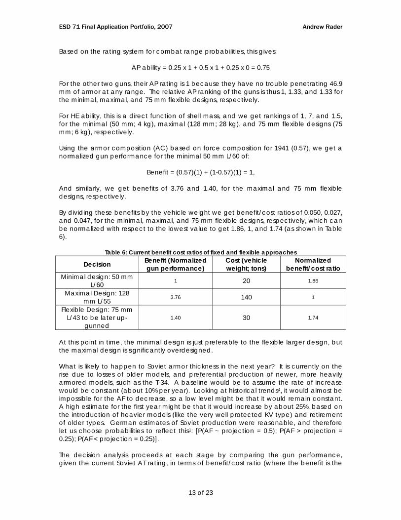
Benefit = (0.57)(1) + (1-0.57)(1) = 1, And similarly, we get benefits of 3.76 and 1.40, for the maximal and 75 mm flexible designs, respectively. By dividing these benefits by the vehicle weight we get benefit/cost ratios of 0.050, 0.027, and 0.047, for the minimal, maximal, and 75 mm flexible designs, respectively, which can be normalized with respect to the lowest value to get 1.86, 1, and 1.74 (as shown in Table 6).

Table 6: Current benefit cost ratios of fixed and flexible approaches

Decision Benefit (Normalized gun performance)

Cost (vehicle weight; tons)

Normalized benefit/cost ratio

Minimal design: 50 mm L/60 1 20 1.86

Maximal Design: 128 mm L/55 3.76 140 1

Flexible Design: 75 mm L/43 to be later up-

gunned 1.40 30 1.74

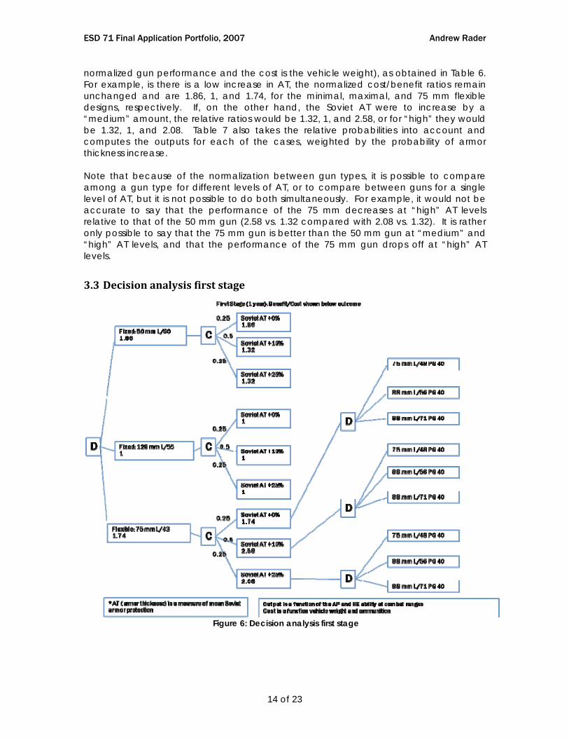
At this point in time, the minimal design is just preferable to the flexible larger design, but the maximal design is significantly overdesigned. What is likely to happen to Soviet armor thickness in the next year? It is currently on the rise due to losses of older models, and preferential production of newer, more heavily armored models, such as the T-34. A baseline would be to assume the rate of increase would be constant (about 10% per year). Looking at historical trends4, it would almost be impossible for the AF to decrease, so a low level might be that it would remain constant. A high estimate for the first year might be that it would increase by about 25%, based on the introduction of heavier models (like the very well protected KV type) and retirement of older types. German estimates of Soviet production were reasonable, and therefore let us choose probabilities to reflect this1: [P(AF ~ projection = 0.5); P(AF > projection = 0.25); P(AF < projection = 0.25)]. The decision analysis proceeds at each stage by comparing the gun performance, given the current Soviet AT rating, in terms of benefit/cost ratio (where the benefit is the


14 of 23

normalized gun performance and the cost is the vehicle weight), as obtained in Table 6. For example, is there is a low increase in AT, the normalized cost/benefit ratios remain unchanged and are 1.86, 1, and 1.74, for the minimal, maximal, and 75 mm flexible designs, respectively. If, on the other hand, the Soviet AT were to increase by a “medium” amount, the relative ratios would be 1.32, 1, and 2.58, or for “high” they would be 1.32, 1, and 2.08. Table 7 also takes the relative probabilities into account and computes the outputs for each of the cases, weighted by the probability of armor thickness increase. Note that because of the normalization between gun types, it is possible to compare among a gun type for different levels of AT, or to compare between guns for a single level of AT, but it is not possible to do both simultaneously. For example, it would not be accurate to say that the performance of the 75 mm decreases at “high” AT levels relative to that of the 50 mm gun (2.58 vs. 1.32 compared with 2.08 vs. 1.32). It is rather only possible to say that the 75 mm gun is better than the 50 mm gun at “medium” and “high” AT levels, and that the performance of the 75 mm gun drops off at “high” AT levels.

3.3 Decision analysis first stage

Figure 6: Decision analysis first stage


15 of 23

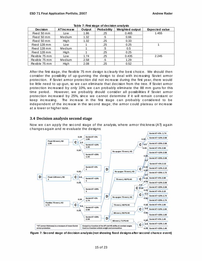
Table 7: First stage of decision analysis Decision AT increase Output Probability Weighted output Expected value

Fixed 50 mm Low 1.86 .25 0.465 Fixed 50 mm Medium 1.32 .5 0.66 Fixed 50 mm High 1.32 .25 0.33

1.455

Fixed 128 mm Low 1 .25 0.25 Fixed 128 mm Medium 1 .5 0.5 Fixed 128 mm High 1 .25 0.25

1

Flexible 75 mm Low 1.74 .25 0.435 Flexible 75 mm Medium 2.58 .5 1.29 Flexible 75 mm High 2.08 .25 0.52

2.245

After the first stage, the flexible 75 mm design is clearly the best choice. We should then consider the possibility of up-gunning the design to deal with increasing Soviet armor protection. If Soviet armor protection did not increase during the first year, there would be little need to up-gun, so we can eliminate that decision from the tree. If Soviet armor protection increased by only 10%, we can probably eliminate the 88 mm guns for this time period. However, we probably should consider all possibilities if Soviet armor protection increased by 25%, since we cannot determine if it will remain constant or keep increasing. The increase in the first stage can probably considered to be independent of the increase in the second stage; the armor could plateau or increase at a lower or higher rate.

3.4 Decision analysis second stage Now we can apply the second stage of the analysis, where armor thickness (AT) again changes again and re-evaluate the designs:

D

Fixed: 50 mm L/601.86

Fixed: 128 mm L/551

C

C

Soviet AT +0%1.86

Soviet AT +25%1.32

Soviet AT +10%1.32

D

Flexible: 75 mm L/431.74

No up-gun- 75 mm L/43

Output is a function of the AP and HE ability at combat rangesCost is a function vehicle weight and ammunition

C

First Stage (2 year): Note: Outcomes from fixed designs not shown

0.25

*AT (armor thickness) is a measure of mean Soviet armor protection

Soviet AT +0%1

Soviet AT +25%1

Soviet AT +10%1

Soviet AT +0%1.74

Soviet AT +25%2.08

Soviet AT +10%2.58

0.25

0.25

0.25

0.25

0.25

0.5

0.5

0.5

D

75 mm L/48 PG 40

D

75 mm L/48 PG 40

88 mm L/56 PG 40

88 mm L/71 PG 40

C

Soviet AT +0%: 1.74

Soviet AT +25%: 2.58

Soviet AT +10%: 2.580.25

0.25

0.5

No up-gun- 75 mm L/43 C

Soviet AT +0%: 2.58



0.25

0.25

0.5

C

Soviet AT +0%: 2.15



0.25

0.5

0.25

CSoviet AT +0%: 2.15


Soviet AT +10%: 1.740.25

0.5

0.25

C

Soviet AT +0%: 1.66



0.25

0.5

0.25

C

Soviet AT +0%: 1.49



0.25

0.5

0.25

No up-gun- 75 mm L/43

C

Soviet AT +0%: 2.58



0.25

0.5

0.25

Figure 7: Second stage of decision analysis (not showing fixed designs after second chance event)


16 of 23

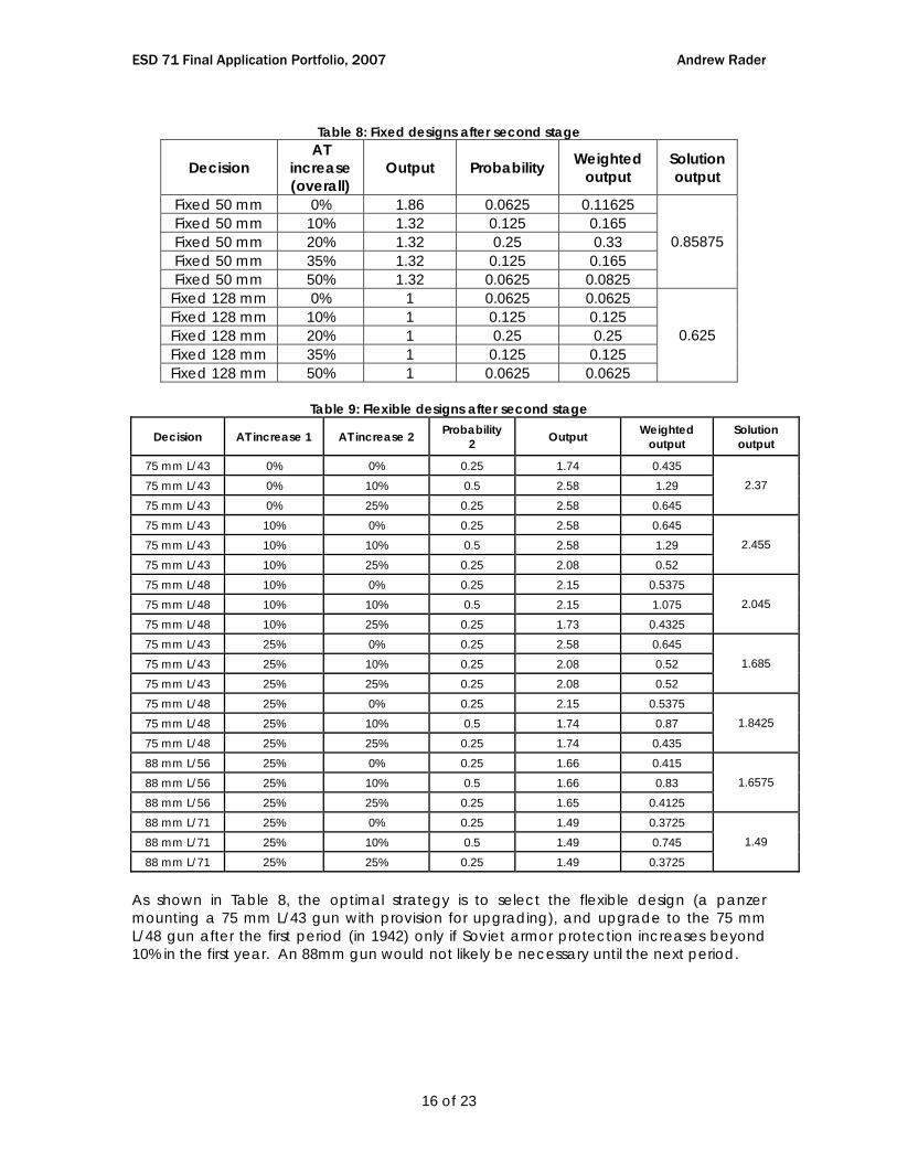
Table 8: Fixed designs after second stage

Decision AT

increase (overall)

Output Probability Weighted output

Solution output

Fixed 50 mm 0% 1.86 0.0625 0.11625 Fixed 50 mm 10% 1.32 0.125 0.165 Fixed 50 mm 20% 1.32 0.25 0.33 Fixed 50 mm 35% 1.32 0.125 0.165 Fixed 50 mm 50% 1.32 0.0625 0.0825

0.85875

Fixed 128 mm 0% 1 0.0625 0.0625 Fixed 128 mm 10% 1 0.125 0.125 Fixed 128 mm 20% 1 0.25 0.25 Fixed 128 mm 35% 1 0.125 0.125 Fixed 128 mm 50% 1 0.0625 0.0625

0.625

Table 9: Flexible designs after second stage

Decision AT increase 1 AT increase 2 Probability 2 Output Weighted

output Solution output

75 mm L/43 0% 0% 0.25 1.74 0.435 75 mm L/43 0% 10% 0.5 2.58 1.29 75 mm L/43 0% 25% 0.25 2.58 0.645

2.37

75 mm L/43 10% 0% 0.25 2.58 0.645 75 mm L/43 10% 10% 0.5 2.58 1.29 75 mm L/43 10% 25% 0.25 2.08 0.52

2.455

75 mm L/48 10% 0% 0.25 2.15 0.5375 75 mm L/48 10% 10% 0.5 2.15 1.075 75 mm L/48 10% 25% 0.25 1.73 0.4325

2.045

75 mm L/43 25% 0% 0.25 2.58 0.645 75 mm L/43 25% 10% 0.25 2.08 0.52 75 mm L/43 25% 25% 0.25 2.08 0.52

1.685

75 mm L/48 25% 0% 0.25 2.15 0.5375 75 mm L/48 25% 10% 0.5 1.74 0.87 75 mm L/48 25% 25% 0.25 1.74 0.435

1.8425

88 mm L/56 25% 0% 0.25 1.66 0.415 88 mm L/56 25% 10% 0.5 1.66 0.83 88 mm L/56 25% 25% 0.25 1.65 0.4125

1.6575

88 mm L/71 25% 0% 0.25 1.49 0.3725 88 mm L/71 25% 10% 0.5 1.49 0.745 88 mm L/71 25% 25% 0.25 1.49 0.3725

1.49

As shown in Table 8, the optimal strategy is to select the flexible design (a panzer mounting a 75 mm L/43 gun with provision for upgrading), and upgrade to the 75 mm L/48 gun after the first period (in 1942) only if Soviet armor protection increases beyond 10% in the first year. An 88mm gun would not likely be necessary until the next period.


17 of 23

4. Lattice Analysis A lattice analysis will be applied to compare the results with the decision analysis (see 3).

4.1 Lattice parameters The main uncertainty in this analysis is the level of Soviet armor protection (mean armor thickness). Soviet armor is expected to increase in any case (as has always been the trend in armored vehicles since they were first developed in the First World War), but the rate of increase is quite uncertain, and there have been periods of virtual stagnation (see Table 1). The mean starting value (at time 0) for AT is 46.9, based on the breakdown of Soviet vehicles in service in 1941 (see 2.5). The expected rate of growth per 1 year period is 25%, with an upper limit of about 100% (doubling every year), and an expected lower bound of 0% (no increase in AT), with about equal base probabilities of occurrence. Our modal forecast is therefore:

Modal forecast = 46.9u = 46.9(e0.25t). For our model, based on historical trends, the armor is more likely to increase than remain constant, but is quite variable, because when a new tank is introduced, it generally incorporates a large armor increase (but generally this is less than once a year). Referring to Table 1 and examining historical vehicles in service with all countries in the Second World War4, we find a very high standard deviation. For the purposes here, we will assume it is 50%, representing a high probability of changing each year (as was historically the case).

p = 0.5 + 0.5 (v/σ)(Δt)0.5 = 0.5 + 0.5 (0.25/0.50) = 0.75 This gives us the following parameters for the lattice analysis:

Table 10: Lattice analysis parameters Parameter Value

Δt 1 year v 0.25 σ 50% u 1.28 d 1.00 p 0.75

4.2 Outcomes and probabilities The lattice method is then applied to determine the “up” (AT increase) and “down” (AT fixed) values and their corresponding probabilities. For example, for the starting AT of 46.90, it has a 0.75 probability of increasing by a factor of 1.28 to 60.03 after the first year, or a 0.25 probability of remaining constant at 46.90. Computing these values for each step in the lattice gives the following outcome (in terms of Soviet AT) and probability (in terms of AT likelyhood) lattices for the next five years (until 1947):


18 of 23

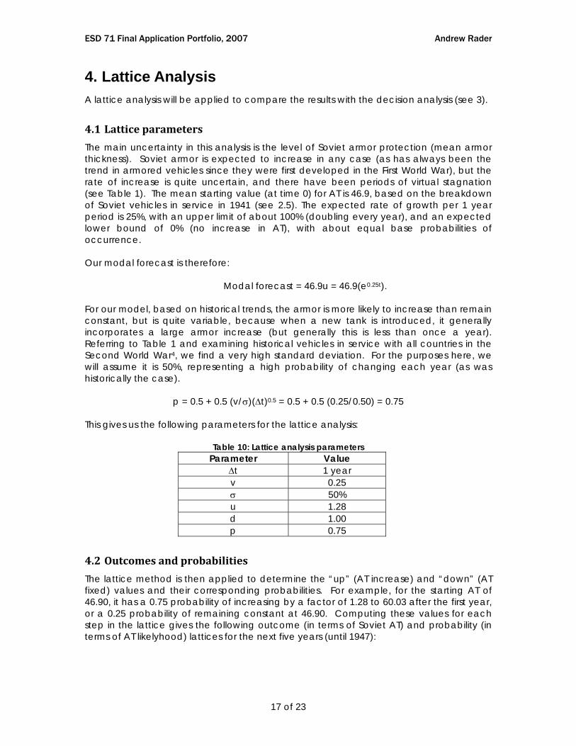
Table 11: Outcome lattice – AT values Step 46.90 60.03 76.84 98.36 125.90 161.15 206.27 6

46.90 60.03 76.84 98.36 125.90 161.15 5 46.90 60.03 76.84 98.36 125.90 4 46.90 60.03 76.84 98.36 3 46.90 60.03 76.84 2 46.90 60.03 1 46.90 0

Table 12: Probability lattice – AT likelyhood Step

1.00 0.75 0.56 0.42 0.32 0.24 0.18 6 0.25 0.38 0.42 0.42 0.40 0.36 5 0.06 0.14 0.21 0.26 0.30 4 0.02 0.05 0.09 0.13 3 0.00 0.01 0.03 2 0.00 0.00 1 0.00 0

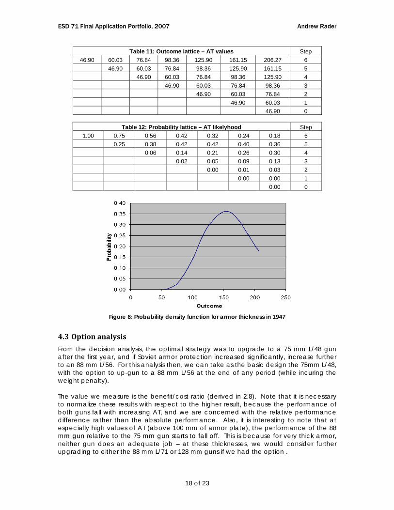
Figure 8: Probability density function for armor thickness in 1947

4.3 Option analysis From the decision analysis, the optimal strategy was to upgrade to a 75 mm L/48 gun after the first year, and if Soviet armor protection increased significantly, increase further to an 88 mm L/56. For this analysis then, we can take as the basic design the 75mm L/48, with the option to up-gun to a 88 mm L/56 at the end of any period (while incuring the weight penalty). The value we measure is the benefit/cost ratio (derived in 2.8). Note that it is necessary to normalize these results with respect to the higher result, because the performance of both guns fall with increasing AT, and we are concerned with the relative performance difference rather than the absolute performance. Also, it is interesting to note that at especially high values of AT (above 100 mm of armor plate), the performance of the 88 mm gun relative to the 75 mm gun starts to fall off. This is because for very thick armor, neither gun does an adequate job – at these thicknesses, we would consider further upgrading to either the 88 mm L/71 or 128 mm guns if we had the option .


19 of 23

Based on the oucome and probability lattices derived in 4.2, and the definitions of benefit/cost ratio derived in 2.8, we can compute the benefit/cost ratios for the 75 mm or 88 mm gun designs at any stage of the lattice. In order to compare the benefit/cost ratios of the guns, they are normalized with respect to the least effective gun for the given AT value, or for the 75 mm gun: Benefit/cost for 75 mm gun lattice = [benefit/cost of 75 mm]/[minimum of benefit/cost of

75 mm or 88 mm gun (whichever is lower for that AT value)].

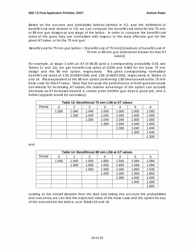
For example, at stage 3 with an AT of 98.36 (and a corresponding probability 0.42; see Tables 11 and 12), we get benefit/cost ratios of 0.034 and 0.063 for the base 75 mm design and the 88 mm option, respectively. This gives corresponding normalized benefit/cost ratios of 1.00 (0.034/0.034) and 1.85 (0.063/0.034), respectively in Tables 13 and 14. This is equivalent to the 88 mm option performing 1.85 times as well as the 75 mm base case for this AT value. Note that because the performance of both guns decrease non-linearly for increasing AT values, the relative advantage of the option can actually decrease as AT increases beyond a certain point (neither gun does a good job, and a further upgrade would be necessary).

Table 13: Benefit/cost 75 mm L/48 at AT values Period 0 1 2 3 4 5 6

1.300 1.040 1.040 1.000 1.000 1.000 1.000 1.300 1.040 1.040 1.000 1.000 1.000 1.300 1.040 1.040 1.000 1.000 1.300 1.040 1.040 1.000 1.300 1.040 1.040 1.300 1.040 1.300

and

Table 14: Benefit/cost 88 mm L/56 at AT values Period 0 1 2 3 4 5 6

1.000 1.000 1.000 1.850 1.540 1.094 1.094 1.000 1.000 1.000 1.850 1.540 1.094 1.000 1.000 1.000 1.850 1.540 1.000 1.000 1.000 1.850 1.000 1.000 1.000 1.000 1.000 1.000

Looking at the overall situation from the start and taking into account the probabilities and outcomes, we can find the expected value of the base case and the option for any of the outcomes in the lattice, as in Tables 15 and 16.


20 of 23

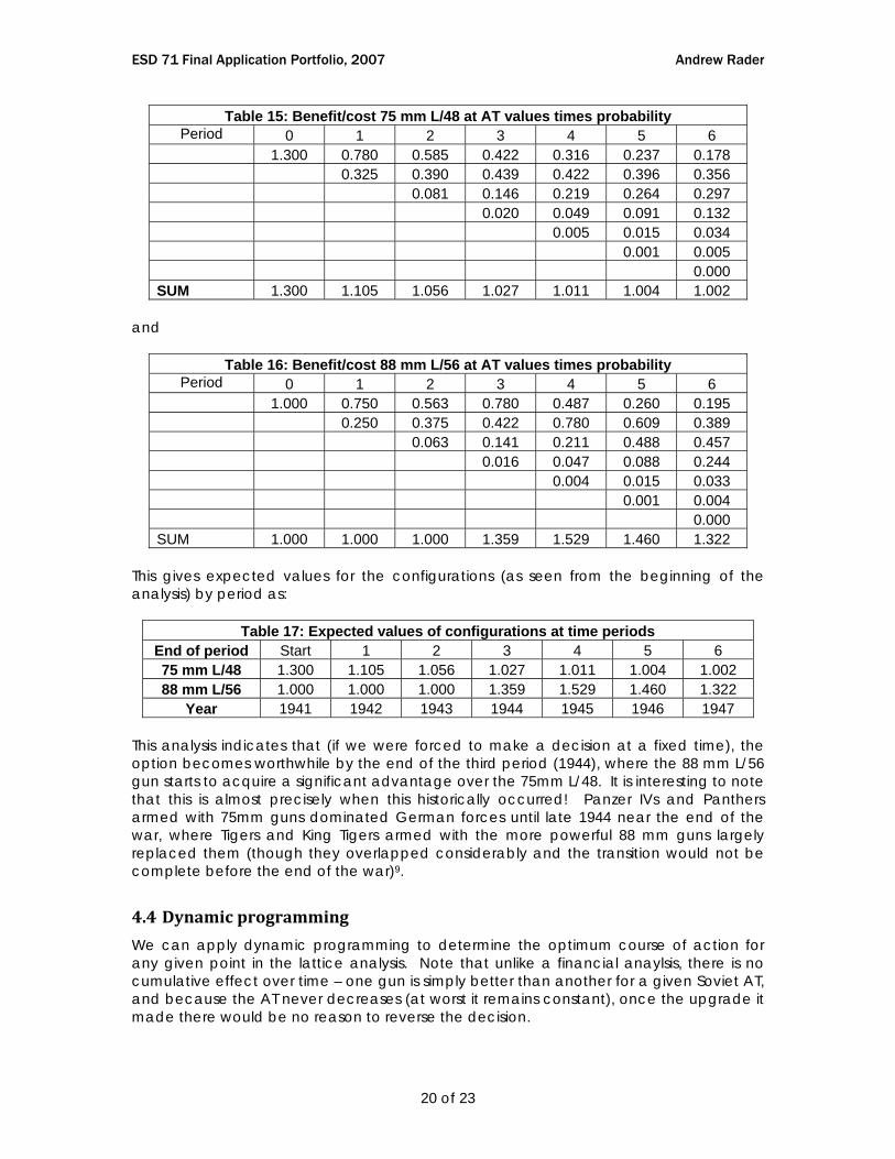
Table 15: Benefit/cost 75 mm L/48 at AT values times probability Period 0 1 2 3 4 5 6

1.300 0.780 0.585 0.422 0.316 0.237 0.178 0.325 0.390 0.439 0.422 0.396 0.356 0.081 0.146 0.219 0.264 0.297 0.020 0.049 0.091 0.132 0.005 0.015 0.034 0.001 0.005 0.000 SUM 1.300 1.105 1.056 1.027 1.011 1.004 1.002

and

Table 16: Benefit/cost 88 mm L/56 at AT values times probability Period 0 1 2 3 4 5 6

1.000 0.750 0.563 0.780 0.487 0.260 0.195 0.250 0.375 0.422 0.780 0.609 0.389 0.063 0.141 0.211 0.488 0.457 0.016 0.047 0.088 0.244 0.004 0.015 0.033 0.001 0.004 0.000 SUM 1.000 1.000 1.000 1.359 1.529 1.460 1.322

This gives expected values for the configurations (as seen from the beginning of the analysis) by period as:

Table 17: Expected values of configurations at time periods End of period Start 1 2 3 4 5 6 75 mm L/48 1.300 1.105 1.056 1.027 1.011 1.004 1.002 88 mm L/56 1.000 1.000 1.000 1.359 1.529 1.460 1.322

Year 1941 1942 1943 1944 1945 1946 1947 This analysis indicates that (if we were forced to make a decision at a fixed time), the option becomes worthwhile by the end of the third period (1944), where the 88 mm L/56 gun starts to acquire a significant advantage over the 75mm L/48. It is interesting to note that this is almost precisely when this historically occurred! Panzer IVs and Panthers armed with 75mm guns dominated German forces until late 1944 near the end of the war, where Tigers and King Tigers armed with the more powerful 88 mm guns largely replaced them (though they overlapped considerably and the transition would not be complete before the end of the war)9.

4.4 Dynamic programming We can apply dynamic programming to determine the optimum course of action for any given point in the lattice analysis. Note that unlike a financial anaylsis, there is no cumulative effect over time – one gun is simply better than another for a given Soviet AT, and because the AT never decreases (at worst it remains constant), once the upgrade it made there would be no reason to reverse the decision.


21 of 23

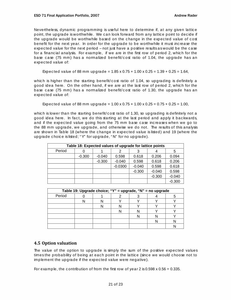
Nevertheless, dynamic programming is useful here to determine if, at any given lattice point, the upgrade is worthwhile. We can look forward from any lattice point to decide if the upgrade would be worthwhile based on the change in the expected value of cost benefit for the next year. In order for the upgrade to be worthwhile it must increase the expected value for the next period – not just have a positive results as would be the case for a financial analysis. For example, if we are in the first row of period 2, which for the base case (75 mm) has a normalized benefit/cost ratio of 1.04, the upgrade has an expected value of:

Expected value of 88 mm upgrade = 1.85 x 0.75 + 1.00 x 0.25 = 1.39 + 0.25 = 1.64, which is higher than the starting benefit/cost ratio of 1.04, so upgrading is definitely a good idea here. On the other hand, if we are at the last row of period 2, which for the base case (75 mm) has a normalized benefit/cost ratio of 1.30, the upgrade has an expected value of:

Expected value of 88 mm upgrade = 1.00 x 0.75 + 1.00 x 0.25 = 0.75 + 0.25 = 1.00,

which is lower than the starting benefit/cost ratio of 1.30, so upgrading is definitely not a good idea here. In fact, we do this starting at the last period and apply it backwards, and if the expected value going from the 75 mm base case increases when we go to the 88 mm upgrade, we upgrade, and otherwise we do not. The results of this analysis are shown in Table 18 (where the change in expected value is listed) and 19 (where the upgrade choice is listed; “Y” for upgrade, “N” for no upgrade).

Table 18: Expected values of upgrade for lattice points Period 0 1 2 3 4 5

-0.300 -0.040 0.598 0.618 0.206 0.094 -0.300 -0.040 0.598 0.618 0.206 -0.0300 -0.040 0.598 0.618 -0.300 -0.040 0.598 -0.300 -0.040 -0.300

Table 19: Upgrade choice; “Y” = upgrade, “N” = no upgrade

Period 0 1 2 3 4 5 N N Y Y Y Y N N Y Y Y N N Y Y N N Y N N N

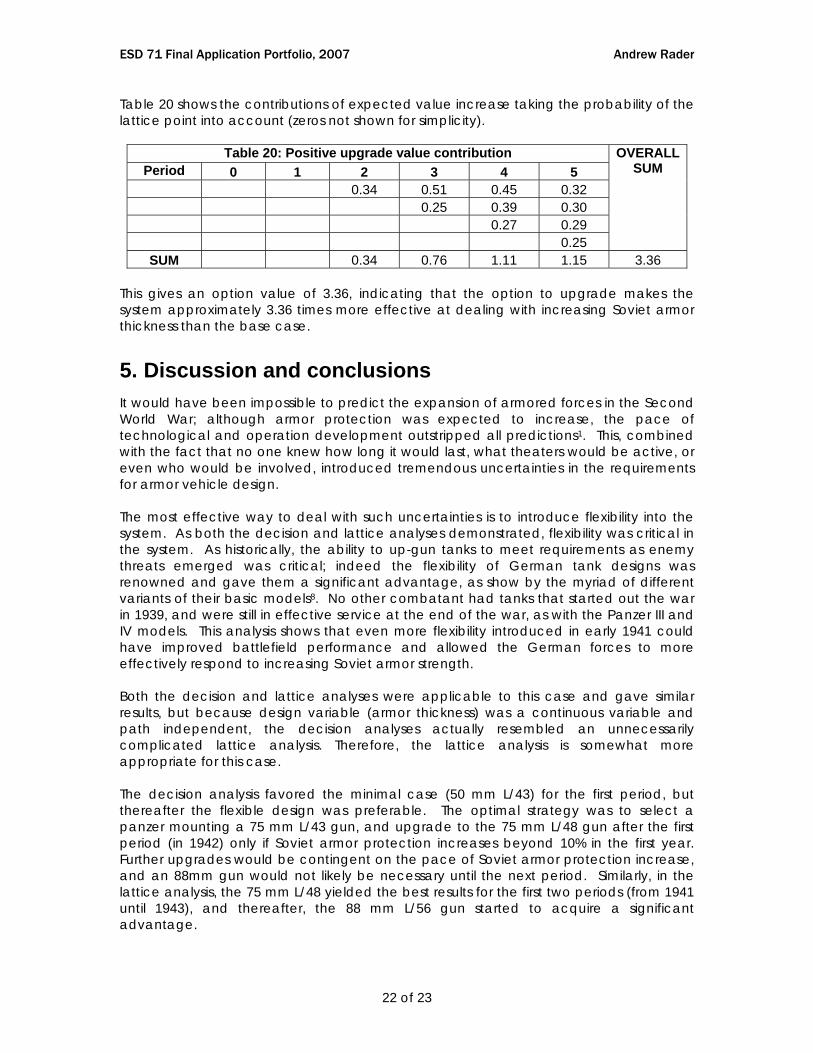
4.5 Option valuation The value of the option to upgrade is simply the sum of the positive expected values times the probability of being at each point in the lattice (since we would choose not to implement the upgrade if the expected value were negative). For example, the contribution of from the first row of year 2 is 0.598 x 0.56 = 0.335.


22 of 23

Table 20 shows the contributions of expected value increase taking the probability of the lattice point into account (zeros not shown for simplicity).

Table 20: Positive upgrade value contribution Period 0 1 2 3 4 5

0.34 0.51 0.45 0.32 0.25 0.39 0.30 0.27 0.29 0.25

OVERALLSUM

SUM 0.34 0.76 1.11 1.15 3.36 This gives an option value of 3.36, indicating that the option to upgrade makes the system approximately 3.36 times more effective at dealing with increasing Soviet armor thickness than the base case.

5. Discussion and conclusions It would have been impossible to predict the expansion of armored forces in the Second World War; although armor protection was expected to increase, the pace of technological and operation development outstripped all predictions1. This, combined with the fact that no one knew how long it would last, what theaters would be active, or even who would be involved, introduced tremendous uncertainties in the requirements for armor vehicle design. The most effective way to deal with such uncertainties is to introduce flexibility into the system. As both the decision and lattice analyses demonstrated, flexibility was critical in the system. As historically, the ability to up-gun tanks to meet requirements as enemy threats emerged was critical; indeed the flexibility of German tank designs was renowned and gave them a significant advantage, as show by the myriad of different variants of their basic models8. No other combatant had tanks that started out the war in 1939, and were still in effective service at the end of the war, as with the Panzer III and IV models. This analysis shows that even more flexibility introduced in early 1941 could have improved battlefield performance and allowed the German forces to more effectively respond to increasing Soviet armor strength. Both the decision and lattice analyses were applicable to this case and gave similar results, but because design variable (armor thickness) was a continuous variable and path independent, the decision analyses actually resembled an unnecessarily complicated lattice analysis. Therefore, the lattice analysis is somewhat more appropriate for this case. The decision analysis favored the minimal case (50 mm L/43) for the first period, but thereafter the flexible design was preferable. The optimal strategy was to select a panzer mounting a 75 mm L/43 gun, and upgrade to the 75 mm L/48 gun after the first period (in 1942) only if Soviet armor protection increases beyond 10% in the first year. Further upgrades would be contingent on the pace of Soviet armor protection increase, and an 88mm gun would not likely be necessary until the next period. Similarly, in the lattice analysis, the 75 mm L/48 yielded the best results for the first two periods (from 1941 until 1943), and thereafter, the 88 mm L/56 gun started to acquire a significant advantage.


23 of 23

It is especially interesting to note that both these analyses followed the historical trend and course of the war – these upgrades are almost precisely in line with historical vehicles. Panzer IVs and Panthers armed with 75mm guns dominated German forces until late 1944 near the end of the war, where Tigers and King Tigers armed with the more powerful 88 mm guns largely replaced them (though they overlapped considerably and the transition would not be complete before the end of the war)9. In fact, this is probably the result of the analyses parameters being framed by historical data, one tremendous advantage not available to historical coutnerparts! The application portfolio excercise was an excellent way to apply the methods learned in class throughout the term to a historical decision. It reinforced both the decision analysis and lattice methods, and indicated how much value can be obtained by incorporating flexibility into a system to tailor the ability and performance of that system to meet the changing (and unpredictable) demands presented in this case by the uncertainties of war.

References [1] Glanz, D. When Titans Clashed: How the Red Army Stopped Hitler. David Glanz. 1998. University Press of Kansas, KS. [2] Ericson, John. The Road to Stalingrad. 1999. Yale University Press, CT. [3] Achtung Panzer: http://www.achtungpanzer.com/stug.htm [4] Ellis, John. World War II: A Statistical Survey: The Essential Facts and Figures for All the Combatants. Facts on File, 1993. [5] The Russian Battlefield: http://battlefield.ru/index.php?option=com_content&task=view&id=34&Itemid=50 [6] KV series: http://en.wikipedia.org/wiki/KV-1 [7] The vehicles: Koenigstiger: http://www.ss501panzer.com/vehicles.htm [8] Chamberlain, Peter. Encyclopedia of German Tanks of World War 2. 1999. Sterling, London. [9] Holborn, Hajo. A History of Modern Germany: 1840-1945. 1982. Princeton University Press, NJ.

design of a replacement german main battle tank in...

Documents