design of a physics abstraction layer for improving the

Design of a Physics Abstraction

Layer for Improving the Validity of

Evolved Robot Control Simulations

Adrian Boeing

This thesis is presented to the

School of Electrical, Electronic and Computer Engineering

for the degree of

Doctor of Philosophy of

The University of Western Australia

By

Adrian Boeing, BE(Hons)

May 2009

ii

The Dean

Faculty of Engineering, Computing and Mathematics

The University of Western Australia

Crawley, Perth

Western Australia, 6009

29th

May 2009

Dear Professor David Smith,

This thesis entitled “Design of a Physics Abstraction Layer for

Improving the Validity of Evolved Robot Control Simulations” is

submitted for the fulfillment of the requirements for the

degree of Doctorate of Philosophy (PhD) at the University of

Western Australia.

Sincerely yours,

Adrian Boeing

iii

Table of Contents

Table of Contents .............................................................................................. iii

Abstract ........................................................................................................... viii

Acknowledgements ........................................................................................... x

1 Introduction .............................................................................................. 11

1.1 Scope .................................................................................................. 14

1.2 Related Work ...................................................................................... 16

1.2.1 Automated Robot Design ............................................................ 16

1.2.2 Crossing the Reality Gap .............................................................. 17

1.2.3 High Fidelity Simulation ............................................................... 18

1.2.4 Minimal Simulation ..................................................................... 21

1.2.5 Hardware In the Loop Simulation ............................................... 23

1.2.6 Hybrid HIL Simulations ................................................................ 24

1.3 Limitations of Previous Work ............................................................. 26

1.4 Combining Multiple Independent Simulators .................................... 29

1.5 Thesis Overview ................................................................................. 35

2 Dynamic Simulation in Physics Engines .................................................... 37

2.1 Solid Body Physics Simulator Paradigms ............................................ 39

2.1.1 Penalty Based Simulation ............................................................ 39

2.1.2 Constraint Based Simulation ....................................................... 42

2.1.3 Impulse Based Simulation ........................................................... 44

2.2 Integrators .......................................................................................... 45

2.3 Object Representation ....................................................................... 49

2.4 Collision Detection and Response ...................................................... 52

2.5 Material Properties ............................................................................ 55

iv

2.6 Multibody Constraints ....................................................................... 56

2.7 Fluid Simulation Paradigms ................................................................ 58

2.7.1 Fluid Effects Modelling ................................................................ 58

2.7.2 Fluid Behaviour Modelling .......................................................... 61

2.8 Dynamics Simulation Summary ......................................................... 65

3 Physics Abstraction Layer ......................................................................... 67

3.1 Previous Approaches ......................................................................... 68

3.2 Software Concepts ............................................................................. 71

3.2.1 Component Based Design ........................................................... 74

3.3 Physics Abstraction Layer Design ....................................................... 76

3.3.1 PAL Object Construction ............................................................. 78

3.3.2 PAL Geometries and Bodies ........................................................ 80

3.3.3 PAL Constraints ........................................................................... 87

3.4 Geometry Representations ................................................................ 87

3.4.1 Terrain Representations .............................................................. 88

3.5 Fluid Model Representations ............................................................. 92

3.6 Actuator Models ................................................................................ 95

3.6.1 Generic Angular Velocity Motor Model ...................................... 95

3.6.2 Generic Angular Position Motor Model ...................................... 96

3.6.3 DC Motor Model.......................................................................... 96

3.6.4 Servo Model ................................................................................ 97

3.6.5 The Hi-Tec 945 MG Servo Model ................................................ 97

3.6.6 Thruster Model ............................................................................ 99

3.6.7 Control Surfaces .......................................................................... 99

v

3.7 Sensor Models .................................................................................. 100

3.7.1 Inclinometer .............................................................................. 100

3.7.2 Gyroscope .................................................................................. 101

3.7.3 Velocimeter ............................................................................... 101

3.7.4 PSD Sensor ................................................................................. 101

3.7.5 GPS ............................................................................................. 102

3.7.6 Contact Sensor ........................................................................... 103

4 Physics Engine Evaluation ....................................................................... 104

4.1 Physics Engine Evaluation Tests ....................................................... 105

4.1.1 Integrator Performance ............................................................. 106

4.1.2 Material Properties ................................................................... 108

4.1.3 Constraint Stability .................................................................... 112

4.1.4 Collision System ......................................................................... 115

4.1.5 Stacking ...................................................................................... 118

4.2 Discussion of Physics Engine Test Results ........................................ 121

5 Evolutionary Control Algorithms ............................................................ 124

5.1 Control System Design ..................................................................... 124

5.1.1 PID Control System .................................................................... 124

5.1.2 Spline Control System................................................................ 126

5.2 Genetic Algorithms ........................................................................... 128

5.2.1 Fitness Functions ....................................................................... 130

5.2.2 Selection Schemes ..................................................................... 132

5.2.3 Genetic Operators ..................................................................... 134

5.2.4 Encoding .................................................................................... 136

vi

5.2.5 Staged Evolution........................................................................ 137

5.2.6 Premature Termination ............................................................. 138

5.2.7 Multi-Objective Optimization ................................................... 139

5.3 Analysis of GA performance ............................................................ 141

5.3.1 Genetic Algorithm Configurations ............................................ 143

5.3.2 Genetic Algorithm Analysis ....................................................... 145

6 Bipedal Robot Control Experiments ....................................................... 149

6.1 Physics Simulation Problems for Legged Robots ............................. 150

6.1.1 Multiple Simulators ................................................................... 152

6.2 Evolving Control Architectures for Bipedal Locomotion ................. 153

6.3 Spline Controller .............................................................................. 157

6.3.1 Sensory Feedback ...................................................................... 158

6.4 Gait Controller Evolved in a High Fidelity Simulator ....................... 160

6.4.1 Target Hardware ...................................................................... 160

6.4.2 Simulation Model ...................................................................... 162

6.4.3 Genetic Algorithm ..................................................................... 163

6.4.4 High Fidelity Simulation Gaits ................................................... 166

6.5 Gait Controller Evolved with Multiple Simulators ........................... 169

6.5.1 Target Hardware ....................................................................... 169

6.5.2 Simulation Model ...................................................................... 170

6.5.3 Evolving the Gait Controller ...................................................... 171

6.5.4 Multiple Simulator Results ........................................................ 173

6.6 Bipedal Robot Control Summary ..................................................... 187

7 Autonomous Underwater Vehicle Control Experiments ........................ 189

vii

7.1 Physical Simulation Problems for Robots in Fluids .......................... 190

7.1.1 Multiple Simulators ................................................................... 192

7.2 AUV Hardware and Simulation Software ......................................... 193

7.2.1 SubSim: An AUV Simulator ........................................................ 194

7.2.2 SubSim Environment ................................................................. 197

7.3 Evolving an AUV Wall Following Controller ..................................... 198

7.3.1 PID Control Algorithm ............................................................... 198

7.3.2 Evolving the AUV Control System ............................................. 199

7.4 Evaluation with Multiple Simulation Systems ................................. 200

7.5 Evaluation with the Mako AUV ........................................................ 203

7.6 AUV Control Summary ..................................................................... 207

8 Conclusion ............................................................................................... 210

8.1 Thesis Summary ............................................................................... 210

8.2 Key Findings ...................................................................................... 212

8.3 Future Work ..................................................................................... 216

9 References ............................................................................................... 219

viii

Abstract

Robots and their control systems are becoming increasingly complex as

growing demands are made for their intelligent operation. Automated design

processes reduce the complexity involved in designing robots, often

leveraging dynamic simulation technology to evaluate potential robot control

system designs. However, physics simulators do not provide a perfect

representation of the real world. Subsequently, control systems designed in a

virtual world will often fail to transfer to the real world.

This thesis presents the design, implementation and evaluation of the Physics

Abstraction Layer (PAL), a uniform component based software interface to

multiple physics engines. PAL can be used to validate the results of an

automated design process, increasing the likelihood that a controller will

function in the real world. All the physics engines fully supported by PAL

were evaluated in a set of benchmarks assessing the key simulation aspects

including friction and restitution models, collision detection and response,

and the constraint solvers. None of the thirteen physics engines evaluated

was found to perform adequately in all aspects. This result indicates that

multiple physics engines should be combined when evaluating a controller

design to achieve valid results.

A genetic algorithm was used to automatically design robot control systems

for two application areas. In the first application, a spline controller was

evolved for bipedal robot locomotion using the PAL’s rigid body simulators

and a high fidelity multibody simulator. The controllers evolved using PAL

outperformed the controllers evolved using previous approaches. In the

second application, a wall following PID control system was evolved for an

Autonomous Underwater Vehicle (AUV). The control systems that were

evolved using multiple fluid dynamics models outperformed all control

ix

systems evolved using either a Lagrangian Smoothed Particle Hydrodynamics

(SPH) model or a Eulerian model.

The biped and underwater vehicle experiments demonstrated that using PAL

to combine physics simulators improved the validity of evolved controllers

for complex robots in dynamic environments. In the future, robot simulation

packages should provide interfaces to multiple physics engines. This would

enable engineers to select the physics engines most appropriate to their task,

and increase the likelihood of a control system developed in a simulator

successfully transferring to the real world.

x

Acknowledgements

First and foremost I must thank my supervisor Thomas Bräunl for all the

feedback and advice he provided, and all the great opportunities and

experiences he has made available over the course of my PhD candidature.

Many thanks to Minh Tran for help with modelling the biped robots and Elliot

and Markus for their work with the AUV robot. Thanks to Brent Fillery, David

Clifton, and my mother for proof reading sections of the thesis and all the

feedback they provided. Thanks to my colleges at ECU and Transmin who

also provided valuable feedback.

Many people from the UWA robotics lab have helped me over the years,

Daniel Venkitachalam, Estelle Winterflood, Andreas Koestler, Joshua Pettit,

Jochen Zimmerman, Steven Hanham, Elliot Alfirevich, Simon Hawe, Pål Ruud,

and Markus Dittmar. Thank you for your help with technical discussions,

support and contributions.

The software developed for this thesis was a large undertaking and I would

like to acknowledge the advice and contributions of the members of the

physics simulation community to PAL including Benoit Neil, David Guthrie,

Volker Darius, Erwin Coumans, Danny Chapman, Dirk Gregarious, Evan

Drumright, Herbert Janssen and many more. They have helped improve the

PAL software, integrated it into many other simulation packages and

provided a great source of motivation.

Finally, this thesis would never have been possible without the loving support

from my friends and family and especially my parents Karl and Marianne, and

my partner Bernadett Szegner.

11

1 Introduction

Robots are becoming progressively more complex and increasing demands

are made for their intelligent operation in challenging environments.

Consequently the control systems for robots have grown exponentially in

complexity from early numerically controlled machines to fully autonomous

robots. As the control system complexity increased engineers started looking

for tools that would assist in the controller design process.

One such tool is virtual prototyping, which enables engineers to rapidly

evaluate new designs using computer based simulations without requiring

intermediary physical prototypes. To date, no simulation has been able to

perfectly reproduce the dynamics of the real world. In practice many

simulators make simplifying assumptions of real world physics in order to

ease the implementation difficulty and improve the computational efficiency.

The discrepancies between the virtual world and the real world can cause

control systems developed in a simulator to perform poorly in the real world.

Rodney Brooks voiced his skepticism regarding the transfer of control

programs from simulations to real robots (1):

“There is a real danger (in fact, a near certainty) that programs which

work well on simulated robots will completely fail on real robots because of

the differences in real world sensing and actuation—it is very hard to

simulate the actual dynamics of the real world.”

This is a sentiment shared by a number of researchers and is widely

acknowledged in the simulation field (2)(3). However, a skilled engineer can

use their previous experience to recognise undesirable and unrealistic results

from a simulation tool and modify their workflow or controller design

accordingly.

12

Even with additional tools the complexity of robotic design is being hindered

by the capacity of engineers to understand the impact of all possible design

variables. As a result a growing body of researchers aimed to create

automated design processes based on the same underlying simulation

technology used in virtual prototyping tools.

Automated design processes generate robot designs by exploring potential

designs based on measurements made from direct design evaluations.

Automated design processes do not have an external source of previous

experience to guide them, so the process learns from thousands of candidate

design trials to generate progressively improved designs. Thus, it must

maximize the reliability of the information gained from each design

evaluation; otherwise it could lead to faulty designs.

The key concern for an automated design process is how the controllers

should best be evaluated. If they are evaluated using real robots in the real

world, then physical robots must be constructed and evaluated in real time.

This would take a prohibitively long time for any automated design process

to generate a controller design, and all the benefits gained from virtual

prototyping approaches would be lost.

An alternative evaluation method is to employ a simulator which can

evaluate the designs faster than real time, without requiring physical robot

construction. However, in evaluating its designs it may come to depend on

characteristics of the simulation that do not match the behaviour of the real

world. Without an alternative means to verify the design, it would be unable

to recognize and correct poor designs that will most likely fail in the real

world.

13

One approach to resolve this is to fuse simulation and hardware approaches

for automated design (4) (5). By validating the simulation’s results on real

hardware the differences between the virtual and real worlds can be

eliminated. However, the reliance on the physical robot’s hardware makes it

difficult to design robots for exotic environments (e.g. space, fluids), and

makes robot structural design changes time-consuming and costly. This limits

the usefulness of these approaches for rapid virtual prototyping.

As an alternative, Jakobi (3) proposed “Minimal Simulation”, an automatic

design approach based purely on limited simulations. This approach focused

on accurately simulating only a few key aspects critical to the target

behaviour of the robot. Although this method has reported a number of

successes, it requires an engineer to select the key simulation features and

build a custom simulator. Furthermore, the simulator is only capable of

generating one behaviour for the robot and can not be generalized. Again,

this makes the automatic development of control systems for complex

robots in complex environments difficult.

For a general automatic design approach to succeed in developing controllers

for complex robots in dynamic environments a complete physics simulation is

required. In order for the controller to operate in the real world, the physics

simulator must provide a mechanism for ensuring that only the valid sections

of the simulator physics are relied upon. This is what this thesis aims to

achieve.

14

1.1 Scope

This thesis addresses the development of a software system and design

technique for automated robot design that allows simulated results to be

reliably transferred to real robots. As stated by Brooks, the key concern is

the differences between the dynamics of the simulation and the real world.

This problem has been studied extensively in the Evolutionary Robotics field.

In this field, the process of transferring a controller from a simulation to a

real environment is often referred to as “crossing the reality gap” (3). Nofi

and Floreano (2) outline three key obstacles to overcoming the reality gap:

1. Different physical sensors and actuators, even if apparently

identical, may perform differently because of slight differences in

the electronics or mechanics, even when exposed to the same

external stimulus.

2. Physical sensors deliver uncertain values, and commands to

actuators have uncertain effects.

3. The body of the robot and the characteristics of the environment

require accurate reproduction in the simulation.

This thesis will focus on the correct reproduction of the robot and

environment. The concerns relating to the uncertainty of the performance

differences in the sensors and the representative noise models have already

been extensively studied by other researchers and will not be investigated

here (2) (3).

Since the aim of this thesis is to create a general approach applicable to any

robot form, a number of physics simulation topics will be addressed including

those concerning rigid body dynamics and computational fluid dynamics.

Some restrictions shall be made on the detail of these simulation models,

15

including aerodynamics, thermodynamics, detailed sensor and actuator

modelling, and power distribution.

As automated design techniques require thousands of design evaluations, it

is important to consider the computational efficiency of the physics engine.

Thus the dynamics models employed will often be simplified models of the

real world, whilst still accepted to be physically valid (6). It is important to

quantify how they approximate the real world’s physics and this topic will be

investigated in depth.

The performance characteristics of the automated design system itself will

not be treated in detail. There is ongoing research into improving the

performance of automated design techniques and evolutionary algorithms,

such as genetic algorithms, and this is largely considered to be beyond the

scope of this thesis.

As this thesis is focused on the valid simulation of the environment and the

robot’s dynamics, the evolved control systems will only consider lower level

locomotion control problems and behaviours. Robot morphology, sensor

and actuator placement, and higher level tasks such as motion planning will

not be considered.

There are several different ways of judging whether a controller successfully

transfers into reality after being evolved in a simulation (3). Some authors

provide direct quantitative comparisons between simulations and reality,

others provide a more subjective view. Generally, the presentation of the

results will depend on the automated design process and robot control task.

The controllers in this thesis will be evaluated according to higher level

quantitative comparisons and qualitative analysis.

16

1.2 Related Work

There have been a large number of attempts at automating an aspect of the

robot design process, with over 100 publications a year since 1997 discussing

an aspect of the process (7). However, relatively few have focused on

overcoming the transitioning of control programs from a simulated

environment to the real world. Of the researchers that do concern

themselves with crossing the reality gap, only a handful deal with robots that

have complex dynamics (3)(8).

Although there have been a number of experiments involving the evolution

of a robot’s morphology, or co-evolution with the control system, there are

only a few software packages that have been made publicly available as a

result of the research work (9)(10).

1.2.1 Automated Robot Design

Automated design processes typically employ an artificial evolution process

to automatically generate a design. To illustrate how this process works, a

simplified example is given (Refer to Chapter 5 for an in-depth treatment).

An artificial evolution process may begin with a set of randomly generated

design candidates. These are evaluated and assigned a score indicating how

close the design candidate is to its goal. The highest scoring candidates are

then reproduced to create a new set of candidates. This process of evaluating

candidates, selecting the best, and creating new candidates is repeated until

eventually the overall goal of the design task is met.

One of the earliest and most widely recognized work in automated design is

Karl Sims work in 1994 on evolving virtual creatures (11). Sims evolved the

morphology and a neural controller for varying locomotion behaviours of

simple computer animated creatures. The software package used dynamic

simulation to calculate the movement of the creatures and had a parallel

17

implementation on a supercomputer to speed up the computation of the

evaluations for the genetic algorithm.

To apply these techniques to robotics requires a more in-depth dynamics

model and sensor and actuator models. In 2000 Leger released a software

package “Darwin2K”(9) that allowed the automatic design of various robots,

including a manipulator and a walking robot for space trusses. Whilst the

dynamics were more complex than that of Karl Sims work, the evolution of

controllers was not addressed, and thus the issues relating to the reality gap

were not investigated.

This has been addressed by more recent approaches that are discussed in the

following sections.

1.2.2 Crossing the Reality Gap

The process of transferring a controller from a simulation to a real

environment is often referred to as “crossing the reality gap” (3). There have

been a number of approaches attempted in solving the problems faced when

transferring control from a simulated environment to the real world. There

have been three main approaches for the transition process:

1. Traditional high fidelity simulation. In the high fidelity simulation

approach the robot is simulated with as much accuracy as possible

and then control programs are tested in the simulation. These control

systems tend to only form the basis for controlling the real robot, and

the control system is essentially re-implemented on the real robot

hardware.

2. Minimal simulation. With this approach only the critical aspects

required to represent a robot’s target behaviour are accurately

modelled. The other aspects are only simulated on a general level, and

the controller is evolved such as to only rely on the critical aspects.

Once the higher-level controllers have been completed in the

18

simulation the lower-level controllers are implemented in the real

world only. This enables the transfer of the high-level control

programs without requiring re-implementation on the real world

system.

3. Robot hardware in the loop. Integrating aspects of the physical robot

with the simulation system allows for a far more realistic

representation of the problem task, allowing a much more accurate

simulation. This approach is similar to the traditional simulation

approach, except that robot hardware is incorporated to improve the

quality of the simulation.

There are advantages and disadvantages to all of these approaches.

1.2.3 High Fidelity Simulation

One of the earliest approaches of developing control systems complex

mechanical robots was the high fidelity simulation approach. McMillan (12)

developed a dynamic simulation software package, “Dynamechs” for land

and underwater robots in 1995. With this software a six legged underwater

walking robot AQUAROBOT(13) was simulated to serve as a testbed for

walking control algorithms.

The control algorithms developed for the AQUAROBOT were implemented

three times, once in a simple forward kinematic simulation, once in the

forward dynamics simulation software developed by McMillan, and finally

again on the physical AQUAROBOT. Although this design process provided a

number of advantages in allowing the researchers to optimize their control

strategies, the inability to directly transfer control algorithms from the

simulation to the real robot meant that only limited testing could be done in

the simulation environment and the controller had to be implemented

multiple times.

19

To enable autonomous design of the robot control systems, the evolutionary

robotics approach was suggested by Husbands and Harvey in 1992 (14). The

need for a simulation environment for this approach was stressed, as many

of the robot designs tested in the simulation would have taken too long to

evaluate on the robot hardware or damage the robot hardware. Husbands

and Harvey acknowledged that the approach would provide only limited

potential on real robot hardware, and proposed the use of adaptive

controllers, such as neural nets to overcome this. Additionally, simulation of

simple robots, lower resolution sensors and using empirical noise data was

suggested.

A number of simulators have also been created specifically for certain vehicle

classes. Stanley et al. (15) evolved a neural controller to serve as an

automobile crash warning system with an open source vehicle simulator.

This control system was then re-implemented on a real mobile robot using

the controller evolved in the simulation as a basis (16). Brutzman(17)

developed an Autonomous Underwater Vehicle simulator and verified the

simulation results using extensive real world test example data.

Typically, the traditional high fidelity simulation approach is not used to

directly transfer final results from the simulation to the target hardware.

Instead, the intermediary results are transferred to the physical robot and

evolution continues on the hardware (2).

Nofi and Floreano (2) outlined the problems associated with crossing the

reality gap for traditional simulations and identified the modelling of the

sensor and actuator behaviour as a key difficulty. Miglino (18) solved this

issue for a two wheeled mobile robot navigation task by recording extensive

data sets for each sensor. The environment was sampled using the robot

hardware, and in the case of distance sensors, each object in the

environment was sampled for 180 orientations and for twenty different

20

distances (2). Miglino noted that the range and angular sensitivity of identical

sensors varied up to two orders of magnitude. There have been claims that

the empirical measurements, whilst quite extensive, were still too coarse

(19). Nevertheless, controllers for morphologically simple robots evolved in

simulations based on this technique continue to perform satisfactorily when

transferred to the real environment (2).

This demonstrated that although it is possible to use high fidelity simulations,

a very accurate empirical model for the sensors and actuators is required.

This limits the application of this technique to simple robots and

environments, as more complex systems become difficult to model due to

the exponentially increased number of situations that need to be sampled

when dealing with multiple situations (2). For example, when considering a

distance reading near two objects, the data must either be re-sampled, or

generated from a summation. This however introduces significant disparities

between the simulation and real environment (2).

To overcome the workload associated with fine grain sampling of real world

systems, mathematical models of the sensor and actuator behaviour can be

constructed instead (2). The mathematical models can be based on known

engineering concepts and the parameters evaluated from empirical data

(19). To alleviate the problems associated with the uncertainty in sensor

readings and actuator commands, noise can be introduced into the

simulation at all levels (2)(19).

Although the traditional simulation approach has had moderate success in

transferring evolved robot controllers to the real world (2)(18)(19), there are

a number of difficulties involved in the approach, including balancing the

level of noise in the simulation (2) and the highly detailed dynamics models

required (1)(2).

21

Lipson and Pollack (20) investigated more complex robot morphologies using

the high fidelity simulation approach for automated design. They evolved the

robot morphology and controllers in a virtual environment, then constructed

the robots using rapid prototyping technology. The evolved controllers were

successfully transferred to the physical robots directly from the virtual

environment. As Lipson et al. assert, the fidelity of the mechanical simulation

will only support simple quasi-static kinematics that can be accurately

predicted (21).

This approach has been shown to have limited applicability to complex

robots due to the complexity involved in constructing an accurate model of

the robot and the environment (21)(22).

1.2.4 Minimal Simulation

The high fidelity evolutionary robotics approach was generally applied to

robots operating in simple dynamics environments and had rigorous

empirical measurements of sensor readings. Furthermore, it was noted that

controllers evolved in simulations would come to depend on particular

aspects only available in the simulation, and hence fail in reality (3). Jakobi et

al. demonstrated that if the noise model is significantly different from the

real system, then the controller is less likely to work when transferred to the

real world (19).

In 1998, Jakobi (3) proposed a solution to these obstacles called “Minimal

Simulation”. This approach attempted to reduce the differences between

simulation and reality by only simulating the aspects of the robot and its

environment that were critical to the success of the control system. These

critical aspects (also known as “base-set” aspects) are reliably simulated and

the aspects deemed to be non-critical (or “implementational” aspects) are

varied for each trial to be unreliable. As a result, controllers only evolve to

depend on the reliable aspects of the system. Furthermore, some variance is

22

introduced to the base-set aspects in order to ensure a robust control system

is evolved (2).

This approach requires a human designer to explicitly identify the robot and

environment base-set aspects, and construct a simulator specific to the task

that models the robot-environment base-set interactions (2). Additionally,

the simulator must feature the implementational, or non-base-set aspects

that do not have a basis in reality.

As a result, the human designer must first assess the problem task to

precisely and accurately identify the reliable, valid behaviour of the system,

and build a simple simulation system that will only allow those behaviours.

Nolfi and Floreano (2) illustrate cases where problems that are decomposed

by Jakobi into base-set and implementational aspects eliminate the

opportunity for some evolvable solutions. This indicates the difficulty of

correctly identifying valid base-set features for any robotics problem,

including relatively simple problems, such as two wheeled mobile robot maze

navigation. Nevertheless, Jakobi successfully applies this method to an

octopod robot by making a number of simplified assumptions regarding the

robot’s dynamics (3).

An octopod robot is statically stable making it relatively simple to control.

Hornby et. al. successfully apply the minimal simulation approach to a more

challenging control task, a quadruped gait controller (23). These successes

indicate the potential for the minimal simulation approach, however Jakobi’s

method is extremely specific to the problem task and assumes that base

assumptions can be made about the problem task to simplify it. This may not

always be the case. For example, in developing a locomotion controller for a

biped there are no simplifying assumptions that can be made regarding the

robot’s dynamics. The entire mechanism must be simulated in order to

determine if the robot is in a balanced state.

23

As a result, the human designer guides the evolutionary process towards a

set of solutions, making the approach more of an optimization task, rather

than an automated design technique (2). Therefore, it is not feasible to

construct a universal evolutionary robotic simulator using the “Minimal

Simulation” approach directly.

1.2.5 Hardware In the Loop Simulation

An early attempt to evolve controllers for legged locomotion was by Lewis et.

al in 1992 (24). To reduce the search space and the cost of evaluating

controller designs the concept of Staged Evolution was introduced. This

allows the robot controller to be evolved over multiple phases, starting with

evolving individual oscillators in the neural net and finishing with the

evolution of the complete gait.

This staged approach was extended by Wilson et al. (25), such that early

phases of the controller evolution were carried out in a simple simulation,

and the final phase was evaluated on real robot hardware. A similar

approach was taken by Miglino et al. (18). These approaches are not strictly

Hardware-In-the-Loop (HIL) simulation, since the simulation phase ends and

then the hardware evaluation begins. There is no interchange between the

simulated controller and the real world controller.

The automotive industry has invested heavily in creating extremely accurate

simulations for a number of automotive components. Kendall and Jones (26)

investigated the differences between traditional simulation, hardware in the

loop simulation, and prototyping approaches for developing control systems

for Ford and Jaguar. They concluded that hardware-in-the-loop simulation

can replace expensive prototypes. However, they require highly detailed

models of the controller’s plant and provided limited usefulness outside of

the plants experimentally verified and predictable input range.

24

Thus, the standard hardware-in-the-loop method suffers from similar

limitations to the traditional simulation approach taken by Miglino et al. in

that second-order and unforeseen environment interactions with the robot

are not possible, as the hardware-in-the-loop is placed in a controlled

environment. Detailed models of the simulated system are still required,

however models and extensive measurements of sensor and actuator data

are not required, as they are directly represented in hardware.

1.2.6 Hybrid HIL Simulations

Zagal et al. (4) proposed a hybrid simulation and real world architecture

named “Back to Reality” (BTR). The key feature of the approach that

minimizes the effect of the reality gap is the co-evolution of the simulation

model with reality. The architecture is depicted in Figure 1, and consists of

three learning algorithms. One for evolving the simulated controller, another

for evolving the physical robot’s controller and finally a learning algorithm for

modifying the simulation model to better fit the real world data. For the

evolution of the robot (in both simulation and reality), the experimenter

provides a fitness function indicating the ability of the controller to achieve

the desired task. The simulation model is evolved based on the average

fitness from both simulation and reality, relative to just the real robot’s

fitness value. In this way, the discrepancies between the simulator and the

real-world are slowly minimized until a controller can successfully cross the

reality gap.

Figure 1 – Back to Reality architecture

Similar to the traditional HIL approach, the BTR approach does not require

extensive real world measurements for th

the BTR algorithm will automatically adjust

match the real-world

require sensor and actuator models in the simulator.

The BTR method was su

behaviour for a quadrupedal robot

successfully transferred to the real robot hardware, making this one of the

few approaches to

system (27).

25

Back to Reality architecture


extensive real world measurements for the sensor and actuator models, as

the BTR algorithm will automatically adjust the simulation parameters to

world. Unlike traditional HIL methods, the BTR approach does

sensor and actuator models in the simulator.

The BTR method was successfully applied for evolving a ball kicking

quadrupedal robot (27). The evolved control system was


to successfully cross the reality gap for a complex robotic


e sensor and actuator models, as

the simulation parameters to

. Unlike traditional HIL methods, the BTR approach does

for evolving a ball kicking

control system was


successfully cross the reality gap for a complex robotic

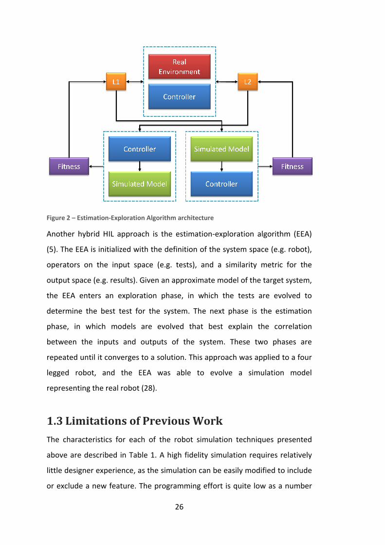
Figure 2 – Estimation-Exploration Algorithm architecture

Another hybrid HIL approach is the estimation

(5). The EEA is initialized with the definition of the system space (e.g. robot),

operators on the input space (e.g. tests), and a similarity metric for the

output space (e.g. results). Given an approximate model of the target

the EEA enters an exploration phase, in which the tests are evolved to

determine the best test for the system. The next phase is the estimation

phase, in which models are evolved that best explain the correlation

between the inputs and outputs of

repeated until it converges to a solution. This approach was applied to a four

legged robot, and the EEA was able to evolve a simulation model

representing the real robot

1.3 Limitations of

The characteristics for each of the robot simulation techniques presented

above are described in Table

little designer experience, as the simulation can be easily modified

or exclude a new feature. The programming effort is

26

Exploration Algorithm architecture

Another hybrid HIL approach is the estimation-exploration algorithm (EEA)

. The EEA is initialized with the definition of the system space (e.g. robot),


output space (e.g. results). Given an approximate model of the target




between the inputs and outputs of the system. These two phases are



representing the real robot (28).

Limitations of Previous Work


Table 1. A high fidelity simulation requires relatively

, as the simulation can be easily modified to include

. The programming effort is quite low as a number

exploration algorithm (EEA)

. The EEA is initialized with the definition of the system space (e.g. robot),


output space (e.g. results). Given an approximate model of the target system,




the system. These two phases are




. A high fidelity simulation requires relatively

to include

quite low as a number

27

of standard CAD tools exist that allow a dynamic model of a robot to be

constructed. However, the detail and complexity required of the model is

quite high. As a result the technique is highly sensitive to discrepancies

between the real world and the simulation, since any error in the robot

model can translate to a significant error in the robot’s dynamics limiting its

applicability to quasi-static mechanisms (21). Finally, due to the complexity of

the model, the computational effort of evaluating the simulation can be

quite large.

High Fidelity

Simulation

Minimal

Simulation

Hardware in the

loop

Designer

Experience

Low Very High High

Model

Complexity

Very high Moderate Low

Programming

Effort

Low High Moderate

Computational

Effort

High Low Low

Sensitivity to

Reality Gap

High Low Low/None

General Robot

Simulation

Yes,

Quasi-static

No,

Simulator specific

No,

Hardware specific

Table 1 – Robot Simulation Techniques

Minimal simulations require extensive design experience, as the robot

designer must be able to specify which aspects of the robot and environment

are to be considered as part of the base-set, and which are not. As a

consequence, the simulation model is often a simplified version of a more

complete traditional high fidelity simulation model, reducing the

computational effort for evaluating the simulation.

28

Differentiating the simulation into base-set and implementational aspects

greatly reduces the processes sensitivity to the reality gap. However, the

simulator must be specifically constructed for the robot and its specific

environment, meaning a significant programming effort is required by the

robot designer for constructing the simulator.

The standard hardware-in-the-loop approach also requires considerable

design experience to know which parts of the robot and its environment to

reconstruct in the physical world and which parts to simulate. As a result, the

model complexity is typically quite low, as the most difficult components to

accurately model are represented in hardware. Therefore, the sensitivity of

the method to the reality gap is either low or nonexistent (depending on the

number of components simulated) and subsequently, the computational

effort in evaluating the model is quite low. Since many of the robot

components are present in hardware, the programming effort is typically

restricted to hardware interface programs and a few simulation components.

The hybrid HIL approaches requires a complete version of the robot

hardware to be constructed, and therefore cannot be used to evolve a

robot’s hardware design. Furthermore, both the EEA and BTR approaches

rely on a single dynamics simulator based on the assumption that it can

accurately model a wide range of situations. This is not necessarily true (29).

For an automated design approach only the traditional high fidelity

simulation approach enables the simulation of any robot morphology,

without requiring extensive designer input or robot hardware. The minimal

simulation approach requires the designer to deconstruct the problem into

base-set aspects, and a standard hardware in the loop approach requires the

appropriate sensors and actuators to be selected and connected to the

simulator. The hardware in the loop method therefore requires at least a

partial construction of the robot. This limits the opportunity for constructing

29

a complete robot design and typically restricts hardware in the loop

autonomous design approaches to optimization of an existing robot design

only.

The minimal simulation approach requires a simulator to be specifically

constructed for the particular task. This severely restricts the solution space

and thereby eliminates the option of an autonomous design of the complete

robot design (e.g. morphology), or of complex dynamical systems. Thus,

minimal simulation is also an inappropriate choice for a general robot design

package.

1.4 Combining Multiple Independent Simulators

This thesis proposes a modification of the traditional high fidelity simulation

approach that makes it more amendable to automated robot design capable

of crossing the reality gap. This is achieved by incorporating aspects of the

minimal simulation approach through the use of multiple independent

physics simulators.

There were two key recurrent themes in the problems highlighted by

robotics and simulation experts (1)(2)(30) with simulations and the reality

gap. These were sensor and actuator noise models and the robot dynamics.

Satisfactory solutions have been proposed for the sensor and actuator noise

models (2)(19).

Jakobi (3) proposes a solution to the robot dynamics problem that is robot,

environment and task specific. The key realization in the minimal simulation

approach was to reduce the simulation to a set of critical aspects (base-set)

that are valid in both the simulation and the real world which the controller

will rely upon, and varying the rest (implementational). However, as this is a

manual process of identifying the base set and implementational aspects,

there is no existing satisfactory general solution for the robot dynamics.

30

This thesis proposes a method for automatically incorporating the base-set

and implementational aspects into a physics simulation. This is achieved by

combining multiple independent simulators, validating each against the

other.

Perfectly modelling any real world feature is not possible, even with careful

empirical validation (3). For example, if the unknown probability distribution

of an underlying real world process is modelled as a normal distribution, then

even if it has the same mean and standard deviation there will be aspects of

this distribution that have no basis in reality (3). Given that there is no

perfect model for a certain physical feature, it will often be implemented

differently for each physics simulator. Furthermore, given that different

simulators are developed with different goals, some simulators may

accurately model one feature, where another simulator makes a simplified

estimation (See Chapter 4 for an analysis of this topic).

As a result, each physics simulator will respond slightly differently for an

identical task due to the differences in the models employed and the

implementation details of the physics engine (See Chapter 2). The aspects

that will behave similarly will effectively form a base-set for the system, and

those that differ, will form the implementational aspects. By using multiple

simulators each aspect will occupy a range across the spectrum from base-

set to implementational, rather than just the binary case.

This concept is illustrated in Figure 3 and Figure 4. Figure 3 depicts a Venn

diagram of the features of the real world and the features of a simulator.

Some properties of the real world will be very accurately modelled by the

simulator. This is indicated by the green Valid region. Some features of the

real world will not be represented by the simulator. This is the red Real

World region. The blue region indicates the section of the simulator that

does not correlate well to the real world.

31

Figure 3 – The overlap between the real world and the simulated world

Any control system developed in the simulator that depends on any of the

features that are only present in the simulated world, will inevitably fail in

the real world. Jakobi’s solution is to manually label the valid, overlapping

region between the real world and the simulator as belonging to the base

set, and the remaining simulated region as implementational.

The solution proposed in this thesis is illustrated in Figure 4. As more

simulators are included in the diagram, the region where each simulator

overlaps is in increasing agreement with the real world. This is represented

by the green Valid region. Thus, the overlapping region can be treated as the

valid base-set, without requiring manual labelling. This is based on the

assumption that each simulator contains a greater region where its

behaviour matches the real world, than not. The regions indicated in the

figure in purple indicate an intermediary between the concept of the base-

set and implementational. This is where two of the three simulators agree

with the real world.

Real

WorldSimulated

WorldValid Simulation

32

Figure 4 – The overlap between the real world and multiple simulators

This concept can be better explained with a concrete example. Consider a

control system for a robot that relies on the timing of a foot striking the

ground. If built in one simulator, the foot will always strike the ground at the

same time. However, a different simulator may consider air resistance, or

employ a less accurate integrator, or employ a more accurate collision

detection mechanism. Each of these aspects will slightly alter the time at

which the floor-ground contact would occur.

The closer the agreement between the simulators on the timing of the foot-

ground interaction, the more the timing can be treated as part of the base-

set. The greater the inconsistencies between the simulators, the more the

timing will be treated as an implementational aspect.

As a result, a controller must be robust enough to cope with slight timing

changes in the foot-ground contact in order to function across all simulators.

It is hypothesized that this degree of robustness will increase the likelihood

of success when transferring across the reality gap. Conversely, in a single

simulator, the controller may come to depend on exactly predictable timing

Real

Sim C

Sim A

Sim BValid

33

for the foot-ground contact, resulting in a controller that would inevitably fail

in the real world.

In this manner the controller is prevented from closely relying on one

particular simulators behaviour. This is further enforced during the

evolutionary process. For each control system, a score is assigned in each

simulator according to how well it accomplishes a task. If one simulator

provides a significantly different response to the others, it is likely the

controller will receive a significantly different score. By employing different

score combining techniques (e.g. average, or median), the influence of this

simulator can be minimized or negated. This requires a modification of the

traditional evolutionary controller design methodology.

The process for the traditional high fidelity simulation approach begins with

the construction of an accurate model of the robot dynamics, the

environment and empirically based sensor and actuator models. The

evolutionary controller design process is then:

1. Initialize a set of potential controller designs

2. Evaluate each design in the simulator

3. Assign a fitness value indicating how well the design solves the desired

task

4. Use an evolutionary algorithm to generate a new set of controller

designs

5. Return to Step 2, until the task is solved.

The proposed extension to this is to evaluate the design not just for one

simulator, but rather on multiple simulators. This would require re-

constructing the robot, environment model, and control program each time

for each simulation system. To remove this time consuming requirement, a

simulation abstraction system is required that can transform a single system

34

representation to a valid representation for various simulators and provide a

single programming interface (See Chapter 3).

With such a system, the initial step in the traditional simulation approach

remains unchanged. A robot designer is still required to construct only one

model of the robot and its environment.

Having multiple simulators alters the evolutionary design process:


2. Evaluate each design in a set of simulators

3. Use statistical methods to assign a fitness value indicating how well

the design solves the desired task

4. Use an evolutionary algorithm to generate a new set of controller

designs

5. Return to Step 2, until the task is solved within a confidence interval,

for all of the simulators

This architecture for the evolutionary design process is similar to the BTR

architecture proposed by Zagal et al. (4) (See Figure 1). In the BTR

architecture the control system is evolved in a simulated environment, and in

the real world. A learning algorithm is used to modify the simulation model

to better fit the real world data. In the proposed multiple simulator

approach, a single evolutionary algorithm evolves a single control system

evaluated in multiple simulators and is coupled with a statistical fitness

evaluation method. This effectively couples the learning algorithm and

evolutionary algorithm structure from the BTR architecture, resulting in a

new architecture that is depicted in Figure 5.

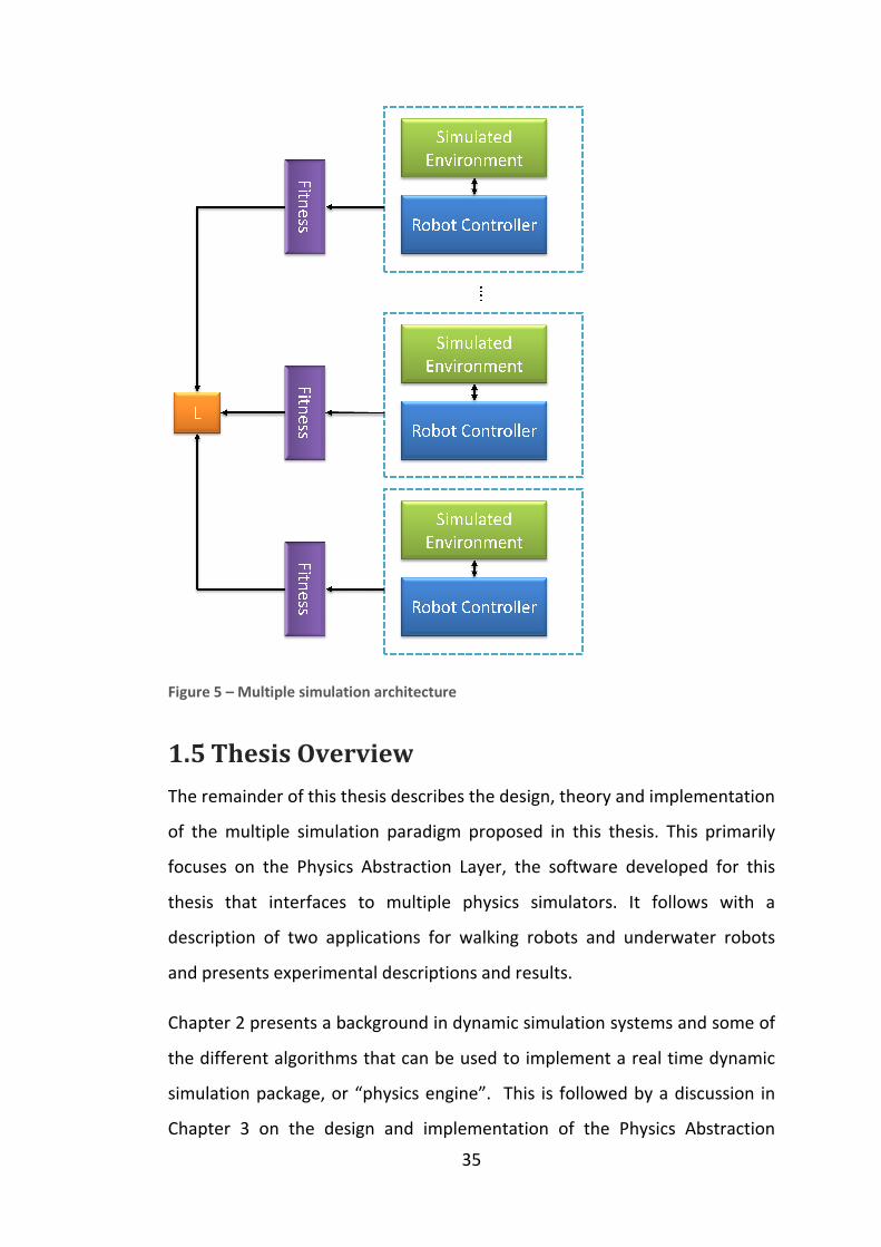
Figure 5 – Multiple simulation architecture

1.5 Thesis Overview

The remainder of this thesis describes the design, theory and implementation

of the multiple simulation paradigm proposed in this thesis. This primarily

focuses on the Physi

thesis that interfaces to multiple physics simulators. It follows with a

description of two applications for walking robots and underwater robots

and presents experimental descriptions and results.

Chapter 2 presents a background in dynamic simulation systems and some of

the different algorithms that can be used to implement a real time dynamic

simulation package, or “physics engine”. This is followed by a discussion in

Chapter 3 on the design and impl

35

Multiple simulation architecture

Thesis Overview



focuses on the Physics Abstraction Layer, the software developed for this



and presents experimental descriptions and results.

pter 2 presents a background in dynamic simulation systems and some of



Chapter 3 on the design and implementation of the Physics Abstraction



cs Abstraction Layer, the software developed for this



pter 2 presents a background in dynamic simulation systems and some of



ementation of the Physics Abstraction

36

Layer, a software package that allows a single robot model and control

system to execute in multiple physics engines in parallel.

Chapter 4 presents an evaluation of multiple physics engines and highlights

the different capabilities of each physics engine and their applicability to

evaluating robot controllers.

An overview of some control systems and genetic algorithms is provided in

Chapter 5. The performance of four different genetic algorithms is

investigated for evolving a walking gait for a simple biped.

Chapter 6 and Chapter 7 assess the transfer of a control system from

simulation to reality using the multiple simulator paradigm and provides a

discussion of the results from a number of experiments. Chapter 6

investigates a gait control problem for a bipedal robot, comparing the

performance between a high fidelity simulation and the multiple simulator

paradigm. The controller for an underwater vehicle is evolved in Chapter 7

and the results from the combined and individual fluid models employed in

the simulation are analysed.

Chapter 8 provides a summary of the contributions and key findings of this

thesis and outlines future opportunities to build on this work.

37

2 Dynamic Simulation in Physics

Engines

Physics engines are software packages that calculate the motion of a system.

Physics engines can simulate a number of different components including

particles, rigid bodies, soft bodies, collisions, constraints, materials and fluids.

Solids such as rigid bodies and soft bodies may all be simulated using the

same techniques, however, fluids may be simulated using techniques

incompatible with standard solid simulation techniques.

Physics engines are not only responsible for maintaining a dynamic model of

the world, but also for performing collision detection, and calculating the

world’s current state given the interactions and constraints between bodies

and the environment.

One of the main tasks of all dynamic simulation systems is to solve the

forward dynamics problem. The forward dynamics problem constitutes

solving for the motion of a system given knowledge of the forces acting on

the system. This can be solved by maintaining the system’s state and

describing its motion with ordinary differential equations (ODE). There are

two basic building blocks for representing dynamics systems(31). Particles,

that can translate and have mass but no volume, and bodies that occupy a

volume and thus can rotate. The state vector of a particle is given in Equation

1, and the state vector for a rigid body is given by Equation 2. The

corresponding motion ODEs are given in Equation 3 and Equation 4

respectively.

=

Equation 1 – Particle state vector (32)

38

=

Where is the particles state vector

is the rigid body state vector

x(t) is the position of the body or particle

v(t) is linear velocity

R(t) is the orientation of the body

P(t) is the linear momentum

and L(t) is the angular momentum Equation 2 – Rigid body state vector (32)

= /

Equation 3 – Particle motion (32)

= ∗

Equation 4 – Rigid body motion (32) =

Where F(t) is the total force on the body

m is the mass of the body is the angular velocity

I(t) is the inertia matrix of the body is the torque acting on the body Equation 5 – Angular momentum (32)

There are a number of factors that influence the characteristics of a physics

engine. These range from the simulation paradigm, collision detection and

response to the type of numerical integrator, or whether air resistance is

considered. As a result each physics engine will provide quite different results

despite simulating the exact same system.

39

Whilst the simulations computational efficiency is of importance,

technological optimizations for various platforms make this a difficult

consideration to thoroughly analyse. This is not of primary concern for this

thesis. Primarily the analysis will concentrate on the simulators capabilities,

robustness and accuracy. Efficiency will only be inspected at a high level. This

chapter provides an overview of the different characteristics that constitute a

physics engine, highlighting aspects that affect its performance.

2.1 Solid Body Physics Simulator Paradigms

There are three major simulator paradigms, the penalty method, constraint

based methods, and impulse based methods (33). Hybrid methods also exist

that combine aspects of the other three in order to try to provide more

functionality or eliminate weaknesses of a particular approach (33) . This

section provides a brief overview of the three methods. The specific details

of each method will be clarified in further sections.

2.1.1 Penalty Based Simulation

The penalty-based simulation approach represents the simulated model as a

collection of particles and spring constraints. All bodies are treated as a set of

particles and interconnecting spring constraints. The interactions between

bodies are represented in the form of temporary spring constraints.

Using a particle system based physics engine with a set of spring constraints

allows the simulation of any meshed shape either as a soft body or as a rigid

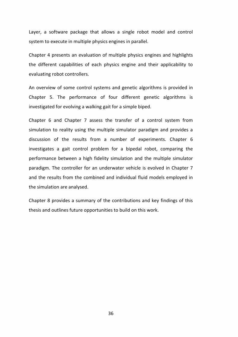
body (depending on the rigidity of the spring constraint). Figure 6 illustrates a

box simulated with the penalty based method. Each vertex of the box is

represented by a free moving particle, and each edge of the box is connected

through a spring. Enforcing the spring constraints such that the springs are

always at their resting length allow the particle-spring system to emulate the

behaviour of a rigid body.

40

Figure 6 – Penalty based method box simulation.

Representing complex shapes using the penalty method results in a large

number of spring constraints. Typically the shape represented in Figure 6

would not contain enough springs for a stable simulation, and additional

cross beam constraints would be added for each surface.

Penalty based approaches use spring constraints to solve object collisions.

When two bodies collide or penetrate, a spring constraint is inserted into the

simulation. The spring constraint is then removed when the bodies are

separating. The spring compresses for a short period of time during the

collision and generates the opposing forces required to re-separate the

bodies. This is illustrated in Figure 7.

41

Figure 7 – Penalty based collision

The key to penalty-based simulation is the representation of the simulation

model as a collection of particles and spring constraints. Spring constraints

can be effectively simulated using Hooke’s Law of elasticity. The general form

of Hooke’s Law is given in Equation 6 and Equation 7.

=

Where is the spring coefficient

and x is the distance from the spring’s equilibrium position Equation 6 – Hooke’s Spring Law =

Where is the damping coefficient

and is the difference in velocity of the spring’s endpoints. Equation 7 - Hooke’s Damping Law

These can be combined to the 3D case as:

= −|| − + ∙ || || Where L is the distance between the two spring endpoints, is the difference between the velocities at the spring endpoints,

and R is the rest length of the spring Equation 8 – Hooke’s Law (3D)

42

Finding a stable and accurate solution to a large number of interacting

penalty constraints is a difficult task. The numerical stability of penalty based

methods is highly dependent on appropriate choices of penalty constants.

This method is simple to implement (including deformable and rigid bodies),

but it is not very robust (33). This makes alternative simulation approaches

attractive for high fidelity simulations.

2.1.2 Constraint Based Simulation

Constraint based methods use analytical constraints to describe the

interactions between objects. An algebraic constraint equation is constructed

to represent the range of valid movements for the body. For example, each

contact constraint is constructed such that each body can only lie on or

above the surface of another body.

The total forces acting on a body can be described as a combination of

independent external forces (e.g. gravity) and the constraint forces (see

Equation 9). There are many different types of constraints (e.g. hinges,

sliders) and different possible formulations (e.g. velocity based). Specific

constraint models are described in Section 2.6.

"# = $% + $&'(

Where "is the bodies mass properties matrix (mass and inertia),

$% are the constraint forces,

and $&'( are the external forces. Equation 9 – Forces acting on a body

The contact and constraint forces can be formulated as a linear system of

equations. The valid directions in which the constraint allows movement can

be encoded into a Jacobian matrix, and the magnitude of the constraint

forces into a scalar vector. This formulation results in Equation 10.

43

$)% = *+,

Where J is the constraint Jacobian

and , is a vector of scalars. Equation 10 – Constraint-based force formulation (34)

Each constraint itself can be formulated as an acceleration constraint. This

can then be solved simultaneously with the motion equation as a system of

equations. The constraint function given in Equation 11 is described in more

detail in Section 2.6.

-. = *# + * = 0

Where - is the constraint function,

Equation 11 – Acceleration based constraint function (34)

" −*+* 0 #, = 0$&'(111111−* 2

Equation 12 – Simultaneous constraints

The constraints affecting a body can be simultaneously solved using an

extended Gauss-Siedel method, or more commonly formulated as a

nonlinear complementarity problem (NCP) (35). Solving these can be

computationally intensive and in some cases may not be robustly solved and

cause physically unrealistic results (36). For example, the Gauss-Siedel

method is an iterative solver, and thus some implementations may choose

not to solve the system completely to reduce the required computation time.

For some cases the constraints may not be solvable at all (37) (See Section

2.5). However, some alternative formulations for constraint based methods

have the benefit of being able to simulate certain common types of multiple

link constraints very accurately.

44

2.1.3 Impulse Based Simulation

Impulse based methods apply impulses to instantaneously change the

velocities of colliding objects. The impulse is calculated in order to prevent

object interpenetration, and obey friction and energy restitution laws. For

example, if two objects collide, an impulse based approach will apply an

impulse in the direction of the contact normal to the two bodies (See Figure

8). This results in a linear and angular impulse on the bodies, altering their

velocities and causing them to separate.

Figure 8 – Contact point and contact normal 3 = 451

Where 3 is the resulting impulse vector

4 is the magnitude of the impulse

and 51 is the contact normal Equation 13 – Collision impulse

To evaluate linked constraints such as ball and socket joints a correcting

impulse is calculated from the relative velocities of the bodies and the

desired relative velocity. The resulting impulse is then applied to the two

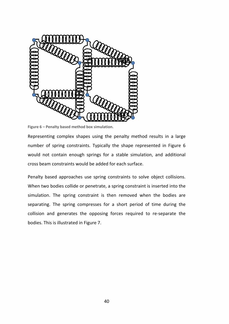
bodies in order to satisfy the constraint. This is illustrated in Figure 9.

45

Figure 9 – Correction impulses

Impulse based methods tend to be faster to compute and simpler to

implement than constraint based methods, but do not handle resting and

continuous contacts well. Unlike the simultaneous constraint based

approach, each constraint is evaluated sequentially contributing impulses to

the final overall movement.

Mirtich provides a comparison of constraint based methods and impulse

based methods in (38), and a comparison of penalty based methods with

constraint based methods is presented by Baraff in (6).

2.2 Integrators

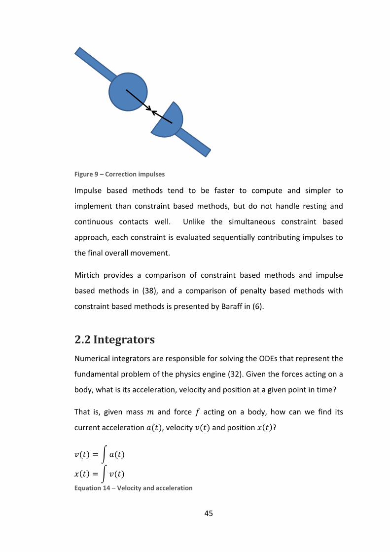
Numerical integrators are responsible for solving the ODEs that represent the

fundamental problem of the physics engine (32). Given the forces acting on a

body, what is its acceleration, velocity and position at a given point in time?

That is, given mass and force $ acting on a body, how can we find its

current acceleration #, velocity and position ?

= 6 #

= 6

Equation 14 – Velocity and acceleration

46

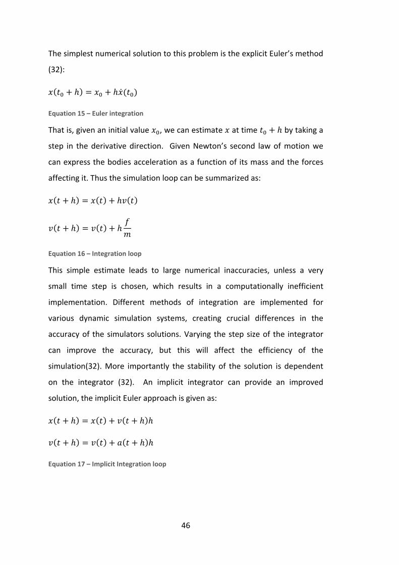
The simplest numerical solution to this problem is the explicit Euler’s method

(32):

7 + ℎ = 7 + ℎ 7

Equation 15 – Euler integration

That is, given an initial value 7, we can estimate at time 7 + ℎ by taking a

step in the derivative direction. Given Newton’s second law of motion we

can express the bodies acceleration as a function of its mass and the forces

affecting it. Thus the simulation loop can be summarized as:

+ ℎ = + ℎ

+ ℎ = + ℎ $

Equation 16 – Integration loop

This simple estimate leads to large numerical inaccuracies, unless a very

small time step is chosen, which results in a computationally inefficient

implementation. Different methods of integration are implemented for

various dynamic simulation systems, creating crucial differences in the

accuracy of the simulators solutions. Varying the step size of the integrator

can improve the accuracy, but this will affect the efficiency of the

simulation(32). More importantly the stability of the solution is dependent

on the integrator (32). An implicit integrator can provide an improved

solution, the implicit Euler approach is given as:

+ ℎ = + + ℎℎ

+ ℎ = + # + ℎℎ

Equation 17 – Implicit Integration loop

47

Implicit integrators are problematic to implement as they require knowing

the future state of the system (34). These can be approximated from the

system state but this is a difficult problem to adequately solve.

A common solution to improving the accuracy of the integrator is to increase

the order of the estimation to include updates at subintervals of the

integration.

7 + ℎ = 7 + ℎ 7 + ℎ92! . 7 + ⋯ + ℎ=5! >=>=

Equation 18 – Taylor series numerical solution to differential equations

A common approach to solve these differential equations is the Runge-Kutta

Method (39). Typically, a fourth order method is implemented as it provides

robust numerical solutions when combined with an adaptive stepping

method (40). This requires the calculation of the force derivatives given the

simulations current state and time, adding further variables into the

implementation. Higher orders are not typically chosen, as it becomes

difficult to describe the higher order movements of the bodies in the system.

The integrator stability problems become paramount during collision

detection. By controlling the step sizes of the integrator an accurate and

efficient simulation can be ensured.

There are three main integrator stepping methods(33). These are fixed time-

stepping methods that update the simulation by a fixed rate, or adaptive

time stepping methods, such as backtracking and time of impact approaches

that alter the time step size to improve the simulators performance.

In fixed-time-stepping, the integrator steps forward by a specified step size

potentially causing overshooting or deep penetrations. This is illustrated in

Figure 10, where a sphere moving toward a cube will have its position

updated, and then collision detection will be performed, resulting in a deep

penetration.

Figure 10 – Fixed time stepping

The backtracking approach

forward and collision detection is performed. If a collision occurs, the time

step is adaptively decreased until the collision states can be correctly solved.

Figure 11 – Backtracking method

Figure 11 illustrates this, before the sphere’s position is updated, a forward

step is taken, a collision test is performed

sphere would penetrate the cube. As a result, the timestep is adaptively

reduced by half. When the physics is updated next, the interpenetration

between the sphere and the cube will be less, resulting in a more stable

simulation.

Time of Impact (TOI) approaches

the simulator keeps track of estimations of the times of impact calculated

from the body’s present velocities and accelerations. The smallest time of

impact is then used to step the simulation forwards.

48


approach(41) is an adaptive solution where a step is taken



tracking method

illustrates this, before the sphere’s position is updated, a forward

, a collision test is performed, and it is determined that




pproaches (38) are another adaptive solution



ep the simulation forwards.


an adaptive solution where a step is taken



illustrates this, before the sphere’s position is updated, a forward

and it is determined that the




another adaptive solution, where



Figure 12 – Time of impact method

In the TOI example illustrated above, before a time step is taken, each

dynamic object calculates the closest distance to the object in front of it. In

this case, the sphere estimates that it will move further in the next time step

than the distance between the sphere and the cube. An estimated time for

the impact is calculated and the simulation is then updated by this time.

The stepping method, integration method, an

the accuracy and robustness of the simulation. An in

effects of the numerical integration method is presented by

(42)

2.3 Object Representation

Each object in the

geometric object. This representation is used during the collision detection

phase to determine when objects are in contact. Additionally, the object

representation may be used to derive physical properties o

as the inertia matrix.

49

Time of impact method



sphere estimates that it will move further in the next time step



The stepping method, integration method, and integration order all affect

the accuracy and robustness of the simulation. An in-depth analysis of the

effects of the numerical integration method is presented by

Object Representation

Each object in the simulation must be represented as some form of



representation may be used to derive physical properties o

as the inertia matrix.



sphere estimates that it will move further in the next time step



d integration order all affect

depth analysis of the

effects of the numerical integration method is presented by Lacoursière in

simulation must be represented as some form of



representation may be used to derive physical properties of the object, such

50

Figure 13 – Convex mesh sphere (left) and mathematically defined sphere (right)

Similar to objects in computer graphics, objects in physics engines are

typically represented as polygonal meshes. However, many simulators

provide special cases for certain geometric objects (See Figure 13). Typical

cases for rigid body simulators are spheres, rectangular prisms, cylinders,

cones, planes, and capped cylinders or capsules. Thus, some simulators may

enable increased efficiency and accuracy by supporting more non-polygonal

geometries. Convex objects (see definition) are generally preferred as they

allow computationally efficient data representations.

Set C is convex if and only if the line segment between any two points in C

lies in C. Equation 19 – Convex object definition (43)

Modern rigid body simulators typically support convex object geometries,

and allow concave geometries to be decomposed into convex objects(44)

that can be combined to provide a concave object representation. This allows

an efficient and accurate solution to collision detection in real time (45).

Typically, these simulators also allow swept geometries, such as those

generated through the Minkowski sum (45), or “dilation” operators. One

advantage of the generation of swept geometries with the Minkowski sum of

convex objects is that the resultant shape is also a convex object (46). This

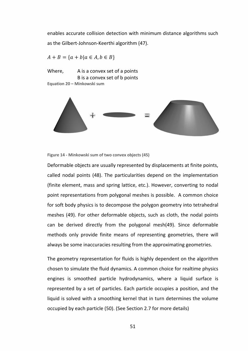
enables accurate collision detection with m

as the Gilbert-Johnson

? + @ = A# + B|# CWhere, A is a convex set of a points

B is a convex set of b pointsEquation 20 – Minkowski

Figure 14 - Minkowski sum of two convex objects

Deformable objects are usually represented by displacements at finite points,

called nodal points

(finite element, mass and spring lattice, etc.). However, converting to nodal

point representations from polygonal meshes is possible. A common choice

for soft body physics is to decompose the polygon geometry into

meshes (49). For other deformable objects, such as cloth, the nodal points

can be derived directly from the polygonal mesh

methods only provide finite means of r

always be some inaccuracies resulting from the approximating geometries.

The geometry representation for fluids is highly dependent on the algorithm

chosen to simulate the fluid dynamics. A common choice for realtime physics

engines is smoothed particle hydrodynamics

represented by a set of particles.

liquid is solved with a smoothing kernel that in turn determines the volume

occupied by each particle

51

enables accurate collision detection with minimum distance algorithms such

Johnson-Keerthi algorithm (47).

C ?, B C @E

A is a convex set of a points

B is a convex set of b points Minkowski sum

Minkowski sum of two convex objects (45)


called nodal points (48). The particularities depend on the implementation



for soft body physics is to decompose the polygon geometry into

. For other deformable objects, such as cloth, the nodal points

can be derived directly from the polygonal mesh(49). Since deformable

methods only provide finite means of representing geometries, there will




smoothed particle hydrodynamics, where a liquid surface is

represented by a set of particles. Each particle occupies a position, and the


occupied by each particle (50). (See Section 2.7 for more details)

inimum distance algorithms such


icularities depend on the implementation



for soft body physics is to decompose the polygon geometry into tetrahedral

. For other deformable objects, such as cloth, the nodal points

. Since deformable

epresenting geometries, there will




, where a liquid surface is

Each particle occupies a position, and the


. (See Section 2.7 for more details)

52

2.4 Collision Detection and Response

The collision phase can be broadly split into two parts, collision detection and

collision response. The collision detection part is purely a computational

geometry problem, formally stated in Equation 21. Although collision

detection is a computationally expensive operation, exact collision detection

for convex objects is possible in real time (45).

? ∩ @ ≠ ∅ ⇔ J C ? − @

Equation 21 – Collision intersection between A and B (45)

Collision detection can be divided into 3 sections:

• Broad phase collision detection, responsible for grouping nearby

objects in order to improve the efficiency of the simulator. This is

achieved through the use of spatial partitioning algorithms.

• Narrow phase collision detection, responsible for determining if two

objects collide. These routines may provide additional information,

such as proximity information for time of impact approaches(33)

• Contact determination, to isolate the geometric areas where two

objects are touching and to perform contact analysis as required by

the simulator paradigm

An example of the broad phase collision detection is illustrated in Figure 15.

The objects in the scene are estimated with axis aligned bounding boxes. If

the boxes overlap, then those objects will pass through to the narrow phase

collision detection. In this example, the cube on the left would not enter the

narrow phase, as its bounding box is not overlapping with any other objects.

The sphere would enter the narrow phase, as its bounding box overlaps with

nearby objects.

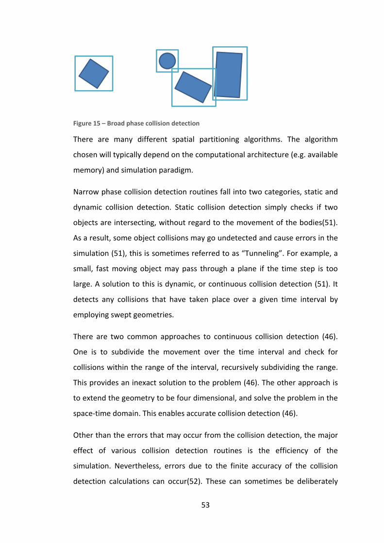
53

Figure 15 – Broad phase collision detection

There are many different spatial partitioning algorithms. The algorithm

chosen will typically depend on the computational architecture (e.g. available

memory) and simulation paradigm.

Narrow phase collision detection routines fall into two categories, static and

dynamic collision detection. Static collision detection simply checks if two

objects are intersecting, without regard to the movement of the bodies(51).

As a result, some object collisions may go undetected and cause errors in the

simulation (51), this is sometimes referred to as “Tunneling”. For example, a

small, fast moving object may pass through a plane if the time step is too

large. A solution to this is dynamic, or continuous collision detection (51). It

detects any collisions that have taken place over a given time interval by

employing swept geometries.

There are two common approaches to continuous collision detection (46).

One is to subdivide the movement over the time interval and check for

collisions within the range of the interval, recursively subdividing the range.

This provides an inexact solution to the problem (46). The other approach is

to extend the geometry to be four dimensional, and solve the problem in the

space-time domain. This enables accurate collision detection (46).

Other than the errors that may occur from the collision detection, the major

effect of various collision detection routines is the efficiency of the

simulation. Nevertheless, errors due to the finite accuracy of the collision

detection calculations can occur(52). These can sometimes be deliberately

54

introduced to increase the computational efficiency of the simulator (45)

(e.g. 24bit floating point verses 32 bit, 64 bit or 80bit).

The contact determination phase can also affect the simulation’s accuracy, as

some simulators develop contacts over time. During sliding contacts, the

geometries contact points may be merge, resulting in inaccurate collisions.

The major factor affecting the accuracy of the simulation with regard to the

collision system is the collision analysis and response. There are three types

of collision contacts (53). Resting contact occurs when two colliding bodies

have a relative velocity of zero (38). If the relative velocity on contact is

positive non zero, then it is a colliding contact (38)(53). Finally, if the relative

velocity on contact is negative, then it is a separating contact.

There are a number of physical properties that can be simulated at the

collision response phase. Common properties are restitution, conservation

of momentum, and frictional forces. The material properties are discussed

later in this Chapter, however, these all effect the calculations during the

collision response phase. When a collision occurs, the total momentum for

both bodies is equal before and after the collision. Equation 22 provides the

collision response for the conservation of momentum.

KL + ML = KN + MN KL + ML = KN + MN

KN = KL + $K 5

Where KN is the velocity of object a after the collision

KL is the velocity of object a before the collision

K is the mass of object a

and n is the collision normal Equation 22 – Conservation of momentum(53)

The method used to simulate the response is dependent on the simulation

paradigm employed. Penalty methods do not set up systems of equations to

55

be solved in the collision response phase, rather, they typically insert new

constraints that allow objects to penetrate, but apply forces that cause the

object to leave the penetrated region. Analytical methods will create an

additional constraint equation as given in Equation 23. - = OMN − OKN ∙ 5

Where - is a velocity constraint Equation 23 – Non-penetration constraint (54)

2.5 Material Properties

Physics engines typically simulate three common properties of materials:

static friction, kinetic friction, and restitution. The material properties help

determine the physics engines response to a collision, in which direction and

at which magnitude the forces are applied.

The coefficient of restitution determines the elasticity of a collision. The

elastic response for two colliding objects is given by:

KN − MN ∙ 5 = −PKL − ML

Where MN is the velocity of object b after the collision

ML is the velocity of object b before the collision

P is the coefficient of restitution Equation 24 – Restitution collision response (53)

The Coulomb model of friction provides an empirical relationship between

normal and friction forces at a contact point (55). The traditional model is

presented below.

= Q=

R = QR=

Equation 25 – Coulomb friction

Where =is the normal force, Q and QR are the static and kinetic friction

coefficients, and and Rare the static and kinetic friction forces. As a force

56

is applied to a body that rests on a surface, the force is initially opposed by

static friction. As the body begins movement, it is opposed by kinetic

friction.

To fit Coulomb’s model to constraint based NCP methods, Coulomb’s friction

cone is often estimated with a friction pyramid, in order to avoid the

nonlinearities defining the quadratic cone constraints (35)(56). A linear

friction collision response is given in Equation 26. Even with linear friction

approximation a correct solution to the LCP cannot be guaranteed (37).

Impulse based methods on the other hand can correctly simulate Coulomb’s

friction model, including transitions between static and kinetic friction (35).

(N = KM − KM ∙ 5

ST%(TU= = QR.KM ∙ 5 − KM

Where ( is the tangential relative velocity

QRis the static friction coefficient

. is the normal component of the relative acceleration

and KMis the relative velocity Equation 26 – Linear static Coulomb friction (53)

2.6 Multibody Constraints

Multibody constraints enable the simulation of different kinds of joints, such

as ball and socket joints or hinges. Two different methods exist for modelling

constraints (57). Reduced coordinate methods restrict the number of

coordinates available to describe a system’s state. Each joint is described in

the coordinate space relative to the previous joint (See (58)). As a result, only

one body in the multibody system has full motion freedom (58). Full

coordinate (or multiplier) methods do not restrict the system state and

instead employ additional forces to maintain the constraints.

57

Reduced coordinate methods achieve very accurate simulation of joints.

Nevertheless, certain joint set configurations such as loops are difficult to

simulate. Full coordinate methods do not restrict the multi-bodies

configuration. However, this means constraints must be continuously

enforced. Thus the method is more susceptible to numerical errors and joints

may begin to drift apart (31).

Constraints are formulated in terms of an implicit position and/or velocity

formulation. They are described by a constraint function, -R. The constraint

function then forms either a position, velocity or acceleration constraint

equation. For example, -R = 0 is a position constraint, whereas -R = 0 is a

velocity constraint.

-R = -R, (, (

Equation 27 –Constraint function

To solve a constraint, we can employ position based, impulse or velocity

based, and force or acceleration based approaches. To obtain a velocity

formulation, the time derivative of a positional constraint is required. This

can be derived using the chain rule:

-R = >-R> = >-R> ∙ >> = *

Where * is the constraint Jacobian matrix. Equation 28 – Velocity constraint formulation

Thus, a velocity constraint can be evaluated from the velocity of a body and

the Jacobian of the constraint equations. The acceleration formulation can be

found from the derivative of the velocity formulation.

-. = *# + *

Equation 29 – Acceleration constraint formulation.

58

Traditionally, the constraint-based simulation paradigm employs reduced

coordinate methods, whereas impulse based methods employ the full

coordinate approach. As a result, impulse based methods cannot efficiently

model tightly constrained joints. However, impulse-based methods can

employ reduced coordinate methods, resulting in a hybrid simulation.

2.7 Fluid Simulation Paradigms

The core difference between traditional rigid body physics and underwater

physics are the liquid effects. These are mostly the drag and lift forces, and

the buoyancy forces. Two approaches to fluid simulation are possible. The

fluid effects themselves can be directly modelled and applied to the bodies.

Alternatively, the behaviour of the fluid itself can be modelled and then the

fluid’s forces can be applied to the bodies.

2.7.1 Fluid Effects Modelling

Directly modelling the fluid forces that are applied to the bodies has the

advantage of being less computationally intensive than fluid modelling

techniques. Many of the forces can be experimentally verified providing an

acceptable model of global effects on a body (59). The interaction of liquid

between multiple bodies is far more difficult to model using direct

techniques, and so it is less appropriate for modelling nearby submersed

bodies (e.g. two ships close to each other).

Buoyancy forces can be calculated from Archimedes' principle. This requires

calculating the volume of a rigid body under the surface of a fluid. This

calculation may require computationally expensive geometry operations.

Alternatively, the volume can be approximated by dividing all volume

structures into smaller spheres that represent the overall shape and volume

of the original structure. For example, a cube structure would be represented

as eight separate spheres that occupy the equivalent volume of the original

59

cube. (See Figure 16) This provides a computationally efficient method for

calculating the buoyancy forces on complex objects and reduces the

complexity of the implementation.

M = (VWX

Where,

V is the volume of displaced fluid

Fb is the buoyancy force

W is the density of the liquid

and g is the gravity force. Equation 30 - Archimedes' principle

Figure 16 - Buoyancy sphere volumes for a cube

The buoyancy force (60) on a sphere is proportional to the volume of the

sphere that is under water. The volume of the sphere that is under the water

is given in Equation 31. From this the buoyancy force can be calculated using

Archimedes' principle given the density of the liquid and the gravity force

(See Equation 30).

V = Yℎ(3[ℎ − ℎ93

Where,

V is the volume of the sphere under the liquid level

h is the height of the sphere that is under the liquid level

and r is the radius of the sphere Equation 31 – Volume of sphere below a given height

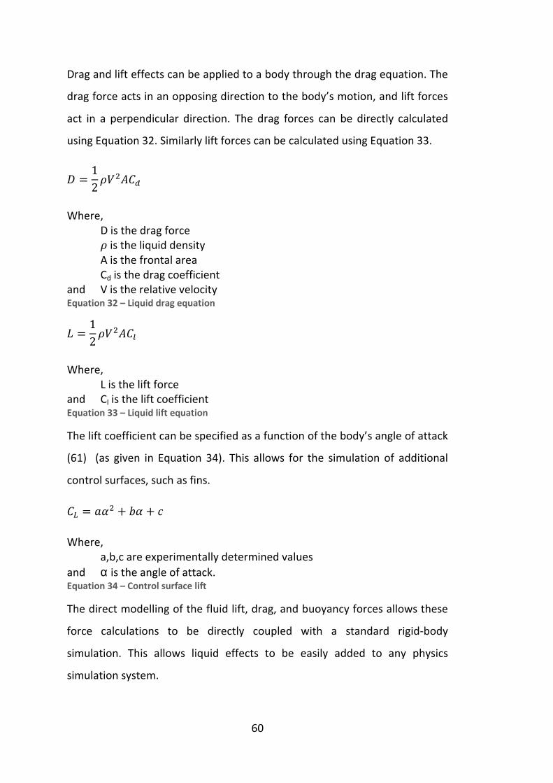
60

Drag and lift effects can be applied to a body through the drag equation. The

drag force acts in an opposing direction to the body’s motion, and lift forces

act in a perpendicular direction. The drag forces can be directly calculated

using Equation 32. Similarly lift forces can be calculated using Equation 33.

\ = 12 WV9?-

Where,

D is the drag force

W is the liquid density

A is the frontal area

Cd is the drag coefficient

and V is the relative velocity Equation 32 – Liquid drag equation

= 12 WV9?-^

Where,

L is the lift force

and Cl is the lift coefficient Equation 33 – Liquid lift equation

The lift coefficient can be specified as a function of the body’s angle of attack

(61) (as given in Equation 34). This allows for the simulation of additional

control surfaces, such as fins.

-_ = #`9 + B` + a

Where,

a,b,c are experimentally determined values

and α is the angle of attack. Equation 34 – Control surface lift

The direct modelling of the fluid lift, drag, and buoyancy forces allows these

force calculations to be directly coupled with a standard rigid-body

simulation. This allows liquid effects to be easily added to any physics

simulation system.

61

2.7.2 Fluid Behaviour Modelling

There are a number of methods for modelling fluids well documented in the

Computational Fluid Dynamics (CFD) literature (62). There are two key

approaches to modelling fluids. Eulerian approaches consider the changes in

a fluid at fixed points, whereas Lagrangian approaches consider the changes

along a trajectory (i.e. a fluid particle). These typically take the form of grid-

based approaches (which subdivides the fluid area into a discrete grid), and

particle based approaches respectively.

Similarly to the solid physics simulation paradigms hybrid or dual approaches

for fluid simulation are also available(63), where both approaches are

combined (e.g. Lagrangian particles exchange fluid information with Eulerian

grids). Whilst there are formulations of both forms that are applicable for

real-time evaluation, particle based approaches enable the simulation of

arbitrary fluid motion of free surfaces in an efficient manner. Due to their

similarities to standard particle based physics approaches discussed in

Section 2.1, these approaches are computationally efficient and straight-

forward to integrate with rigid body and soft body systems. Conversely, grid

based approaches can be memory intensive and thus efficient real-time grid

based approaches tend to be two dimensional.

Most fluid models are based on Euler’s fluid dynamics equations or

extensions thereof. These equations are formulated from the pressure

changes of Newton’s second equation applied to a fluid element (64).

Assuming incompressible fluids this results in Equation 35.

62

W >> + ( ∙ ∇ = −∇p

∇ ∙ = 0

Where W is the density,

v is velocity,

p is pressure,

and ∇ is the spatial gradient operator. Equation 35 – Euler’s fluid dynamics equation

Euler’s equation ignores friction between water molecules, Navier-Stokes

equations extend the Euler equations to consider the fluids viscosity. These

equations form the basis of most fluid models.

W >> + ( ∙ ∇ = −∇p + μ∇9 + Ffghfijkl

Where μ is the kinematic viscosity Equation 36 – Naiver-Stokes equation

A simplified model for the movement of fluid surfaces are dampened shallow

water equations (64)(65). The shallow water equations assume an

incompressible, in-viscid fluid and ignore vertical acceleration on the

assumption of large scale motion slowly varying motion. The equations are

formulated based on the waters height from the ground.

>m> + X >ℎ> = 0, >> + X >ℎ>n = 0, >ℎ> + ℎ >m> + >>n = 0

Where u and v are the fluid velocities in x and y directions

h is the height of the water surface

and g is gravity. Equation 37 – Simplified shallow water equations

A finite difference using central approximations can be used to evaluate the

shallow water equations efficiently on a 2D grid. This results in a surface that

simulates a body of water. To interact with rigid bodies, the fluid’s buoyancy

force must be calculated. This can be achieved by using the discretized

approximation and treating each location in the grid as a column of water.

63

Rigid bodies are then sampled using raycasting to determine the proportion

occupying the underwater volume. The amplitude of the surrounding water

can then be altered according to the forces of the body on the fluid. Figure

17 illustrates the volume of a submersed body and floating body on the

discretized fluid surface.

ℎT,o(N∆( = ℎT,o( + (1 − ∆qℎT,o( − ℎT,o(L∆(r

+ ∆(s%s∆'s (4ℎT,o( − ℎTNu,o( − ℎTLu,o( − ℎT,oNu( − ℎT,oLu(

Where is the water damping constant

and c is the wave speed Equation 38 – Discretized two dimensional wave equation

Figure 17 – Buoyancy column

An alternative to grid based approaches are particle based approaches. The

most common real-time implementation of 3D fluid motion is the Smoothed

Particle Hydrodynamics (SPH) method. The SPH method evaluates field

quantities anywhere in space based on a set of discrete particle locations.

Each particle represents a certain volume of space and influences

neighbouring particles through a smoothing function, or smoothing kernel

Water surface

Rigid Body

Water

Occupied

Volume

(see Figure 18). Substituting the Navier

of the SPH smoothing functions provides the acceleration of a particle inside

a fluid. This allows the evaluation of the pressu

tension of a fluid, directly creating the resulting forces required to affect a

body interacting with a liquid.

a SPH particles location.

Figure 18 – Smoothed Particle Hydrodynamics smoothed influence

WT = v oow(T − o , ℎ

Where ρ is the particles density,

m is the particles mass,

W is the smoothing kernel,

x is the particles position,

and h is the influence radius.Equation 39 – SPH density equation

From the density both the pressure force and viscosity forces can be

calculated. Buoyancy forces emerge from the system as a result of the

density of the particles.

64

). Substituting the Navier-Stokes equations into the Laplacian


a fluid. This allows the evaluation of the pressure, viscosity and surface


body interacting with a liquid. Equation 39 calculates the density of a fluid at

Smoothed Particle Hydrodynamics smoothed influence

is the particles density,

m is the particles mass,

W is the smoothing kernel,

the particles position,

h is the influence radius. SPH density equation


calculated. Buoyancy forces emerge from the system as a result of the

Stokes equations into the Laplacian


re, viscosity and surface


nsity of a fluid at


calculated. Buoyancy forces emerge from the system as a result of the rest

65

$T&x& = − v o yT − yo2Woo∇wqT − o , ℎr

Where p is the particles pressure. Equation 40 – SPH pressure force

$TzT%UT( = Q v o T − oWoo∇9wqT − o , ℎr

Where µ is the viscosity coefficient

and v is the particles velocity Equation 41 – SPH viscosity force

Finally the pressure term is calculated from Equation 42.

y = (W − W7

Where k is the gas constant

and W7 is the rest density. Equation 42 – Modified ideal gas equation

2.8 Dynamics Simulation Summary

There are a wide variety of design choices available to dynamic simulation

developers. Furthermore, hybrid algorithms can be implemented that inhibit

varying advantages and disadvantages from the standard algorithms

described above. Simulation designers need to balance the tradeoffs

between various design choices, and can at best only implement a solution

that provides ideal performance for a particular problem, and not as a

general dynamic simulation framework. As a result the accuracy, robustness

and efficiency of a complete dynamics simulation package will vary greatly.

Each of the simulation attributes described in this chapter are valid

interpretations of the models that represent the physical reality of the

system. There is no clear method for determining which particular physical

simulation model will best suit a particular robot control problem. Thus, a

simulation developer is forced to choose one particular method and assume

66

that it will provide the best results for the system they wish to simulate. If

the chosen simulation paradigm does not capture all of the essential

elements of the robot and its environment, then the simulation may lead to

invalid results.

67

3 Physics Abstraction Layer

The software developed for this thesis can be broadly broken into five

separate forms:

• A component based dynamics simulation abstraction framework, for

robustly simulating various physical aspects

• A control library, for controlling the robot’s actions

• An evolution library, for evolving control structures

• A graphics library, for displaying simulation results

• Application specific code, for accomplishing the tasks of the

application

The main focus of this thesis concerns the design of the dynamics simulation

software abstraction framework. The control library, evolution library, and

graphics library each contain a set of functions that assist the programmer in

achieving their goal. The application specific code is of a different nature for

each application, and this code leverages the capabilities presented by the

other software libraries.

In this chapter the design of the Physics Abstraction Layer (PAL) is discussed.

It begins with an overview of some architectures for representing robotic

mechanisms and the requirements for the design of a software abstraction

layer. This is followed by a discussion of some common software design

concepts. Finally, the design and implementation of the PAL software

developed for this thesis is presented.1

1 Note: PAL is open source software, the entire PAL software plus the COLLADA and Scythe loaders

are available from http://pal.sourceforge.net/

68

3.1 Previous Approaches

An abstraction layer is a set of generalizations of models or algorithms away

from their specific implementation details. Supporting a number of different

physics engines within one application requires an abstract system

architecture for representing the contents of the virtual world and

interacting with them. There have been many approaches to abstract

modelling of robotics mechanisms for multibody simulation (66)(67). An early

approach was the Dymola system, a language for describing robot

mechanisms and their interactions. This specification was then compiled to a

target language. Whilst capable of representing a wide variety of

mechanisms, the system operated on a very low level, producing the

differential equations required to solve each component. This drawback with

this type of framework is that it is very difficult to extend it to support

interactions with other complex systems, such as modern collision detection

libraries.

Newer approaches include the Open Robot Control Software (ORCOS) project

(67), which provides a modular framework for robot control. This is largely

based on the “Object-Port-Connector” design pattern. Objects represent

physical mechanical components, connectors represent kinematic and

dynamic constraints, and ports represent the interaction points.

Another framework is NASA’s Coupled Layered Architecture for Robotic

Autonomy (CLARAty) unified mechanism model (67). It contains four key

software abstractions, a body, a joint, a mechanism model and a mechanism

interface. CLARAty Bodies represent rigid bodies and the joints represent the

kinematic relationship between them. The CLARAty bodies can encapsulate

the joints into one structure. The Mechanism Model encapsulates the bodies

and joints into a complete tree structure to represent the robot’s topology.

69

Finally, the mechanism interfaces represent the portions of the mechanism

that can be manipulated.

The abstract model approach taken by CLARAty provided a good starting

point for constructing an abstract representation of a simulator-independent

software, whereas the retargeting approach taken by Dymola enables more

specific features to be incorporated. NASA’s CLARAty provided support for

multiple physics simulation approaches through a uniform abstract interface

based on the adapter design pattern. The adapter design pattern adapts one

interface to a class into another application’s uniform definition (68). The use

of this pattern enables all simulations to be treated in a uniform manner, and

this formed the basis of the design inspiration for PAL.

During the development of the software for this thesis three projects for

providing abstract representations for physics engines were initiated. In 2004

the Open Physics Abstraction Layer (OPAL) (69) began development. This

project was based on similar concepts as the Physics Abstraction Layer (PAL)

software developed in this thesis, and inherited its name from PAL. Unlike

PAL, OPAL only provided support for one physics engine, and acted as a

higher level interface rather than an abstraction layer. As PAL improved the

OPAL project was abandoned. Since OPAL inherited its name and shared

much of its architecture from PAL it will not be discussed in detail.

In 2005 the COLLADA consortium released v1.4 of their COLLADA file format

specification that included physics support (70)(71). COLLADA only provides a

file format for representing physics models, and does not provide an

application programming interface (API) for interacting with the file format.

Thus, any programs that are written to support COLLADA still need to

develop specific code for each physics engine to achieve the applications

goal. Nevertheless, the COLLADA file format influenced the design of the PAL

6DOF constraint.

70

The GangstaWrapper (72) was released in 2005. It made heavy use of the

adapter design pattern and shared many design decision similar to those

taken in the design of PAL despite having independent origins.

GangstaWrapper was only designed to support modern full featured physics

engines and lacked the backwards compatibility design aspect of PAL. The

GangstaWrapper did influence some of the design aspects of PAL’s support

for modern collision detection systems.

None of the previous physics abstraction approaches provided an extensible

and flexible design architecture for dynamically supporting multiple physics

engines. This can be attributed to the fact that most of the previous

approaches did not aim to support very many independent physics engines

(GangstaWrapper supports the most: four), making hard-coding of the

engine support feasible. This is very different from the design goals of PAL

which aims to support as many physics engines as possible (PAL currently

supports 13 engines).

As consumer level dynamic simulation engines are an emerging technology,

the engine designs are constantly evolving. In order to keep pace with the

ever changing simulation technology and still maintain compatibility a plug-in

system is required (73). Plug-ins are a common software development

technique that allow a software application to provide extended functionality

on demand. To enable the programmer to construct and interact with PAL

without requiring access to a concrete implementation, the abstract factory

pattern (68) can be combined with the plug in approach cumulating in the

abstract pluggable factory (See Section 3.2 for an in-depth explanation). This

pluggable factory based design delivers all of the component requirements:

• uniform interface to multiple software libraries

• extensible, versioned classes

• adaptable, able to dynamically construct concrete objects

71

The use of the abstract pluggable factory enables comparative compile-

specific functionality as offered by the Dymola abstraction language.

For the evolutionary algorithm to be able to connect and configure a large

number of objects some form of standard communications interconnection

between the objects is required. A motor must be controllable from a control

algorithm whether it be a PID or Fuzzy control, and regardless of whether the

control algorithm utilizes a PSD sensor or an inclinometer as its input. To

achieve this level of flexible interaction a communications standard between

the control algorithms, sensors and actuators needs to be established. This is

achieved through a component based dataflow design (74) (See Section

3.2.1). By developing a set of standard interconnecting components on top of

the abstract pluggable factory a system is realized where the information

flow can be managed and reconnected between components, without regard

to the specific simulation environment or targeted hardware. This enables a

more abstract version of the Port-Connector concept of the ORCOS

framework.

3.2 Software Concepts

For any large-scale software system an appropriate platform is required for

efficient development. In order to develop software that is able to provide

abstract access to a number of systems in an efficient manner a component-

based framework was developed.

Software components differ from software libraries, in that libraries are a

collection of subprograms which present useful functions for the application

software. Frameworks however provide a set of interoperating abstract

classes that provides a reusable design for a specific type of software (75).

Component based software defines a basic communications system enabling

software classes to be a single versioned deployable unit (74).

72

An abstract pluggable factory(73) provides three key features:

1. A central repository to construct objects

2. The ability to plug in custom objects or extend existing versioned

objects

3. A uniform abstract interface to the concrete implemented objects

These features are key requirements for constructing a component-based

framework.

A software factory class offers a set of services for generating instances of

various subclasses without explicitly requiring the name of the class we wish

to construct(68). A pluggable factory expands this concept by allowing plug-

ins to automatically extend the application’s functionality without requiring

any modifications to the application code itself.

To implement a pluggable factory the factory class requires a registry that

maintains a list of all available components, and a method for creating a

component. When a component is created, the factory can search through

the registry for the desired class type, construct it, and return it for use. Each

class that needs to be accessible via the factory requires a method that

allows a copy of itself to be created, as well as a method to add its

information to the factories registry. By creating a static copy of the class, the

information is automatically registered at the very beginning of the

application, before any user code is executed. Implementation details of this

approach for C++ are provided in Culp(76).

The basic abstract pluggable factory design was extended in this thesis with

novel additions allowing the construction of classes from shared objects

(DLLs) and encapsulated the class registration information into a separate

structure to allow versioning of objects. This registration information can

then be employed to group objects or select the correct version of a class to

73

construct (e.g. Construct version three, not version two). A UML diagram of

the pluggable factory pattern is depicted in Figure 19, and the pseudo code

implementation for this approach is given in Listing 1.

Listing 1 - Pseudo code for a pluggable factory

struct RegistrationInfo /* registration information */

string className int version FactoryObject *pConstructor class FactoryObject FactoryObject /*constructor*/ Factory::registry.add(

/*this classes information*/ ); FactoryObject *Create()

/*return a new copy of this class*/ return new FactoryObject; static const FactoryObject registerThis; ; class Factory FactoryObject *CreateNewObject( string name) FactoryObject *object = find(name, registry);

/* find an object which uses this name in the registry*/

return object->Create(); /* call the create function of the object, to return a new copy for our use*/

static list <RegistrationInfo> registry;

/*the list of registered components*/

74

Figure 19 – UML diagram for a pluggable factory

Figure 20 – Sequence diagram for a pluggable factory

Figure 20 depicts a sequence diagram for the registration of objects into the

factory and the creation of new objects from the registry. Initially a static

version of each object is constructed. In the constructor the concrete object

calls the factory object which in turn calls the add method of the factory. This

ConcreteFactory

+CreateProductA()+CreateProductB()

AbstractProductA

+Create()

ConcreteProductA

+RegistrationInfo

+Create()

AbstractProductB

+Create()

ConcreteProductB

+RegistrationInfo

+Create()

AbstractFactory

+Registry: RegistrationInfo

+CreateProductA()+CreateProductB()

Client

ConcreteObject FactoryObject Factory

ConcreteObject()

Add()

CreateNewObject

Find()

Create()new

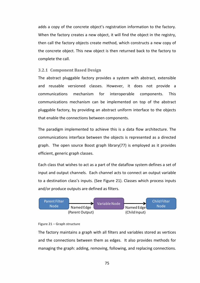
75

adds a copy of the concrete object’s registration information to the factory.

When the factory creates a new object, it will find the object in the registry,

then call the factory objects create method, which constructs a new copy of

the concrete object. This new object is then returned back to the factory to

complete the call.

3.2.1 Component Based Design

The abstract pluggable factory provides a system with abstract, extensible

and reusable versioned classes. However, it does not provide a

communications mechanism for interoperable components. This

communications mechanism can be implemented on top of the abstract

pluggable factory, by providing an abstract uniform interface to the objects

that enable the connections between components.

The paradigm implemented to achieve this is a data flow architecture. The

communications interface between the objects is represented as a directed

graph. The open source Boost graph library(77) is employed as it provides

efficient, generic graph classes.

Each class that wishes to act as a part of the dataflow system defines a set of

input and output channels. Each channel acts to connect an output variable

to a destination class’s inputs. (See Figure 21). Classes which process inputs

and/or produce outputs are defined as filters.

Figure 21 – Graph structure

The factory maintains a graph with all filters and variables stored as vertices

and the connections between them as edges. It also provides methods for

managing the graph: adding, removing, following, and replacing connections.

Parent Filter

Node

Child Filter

NodeVariable Node

Named Edge

(Parent Output)

Named Edge

(Child Input)

76

The filter classes themselves maintain a list with their accepted input and

output formats.

The factory class is also responsible for managing data flow during execution.

The graph is traversed in a modified breadth-first search such that each filter

operates on its input data, passes the results to a variable node, which in

turn is read by the next filter, operated on and passed down the graph to the

final terminating nodes to perform an action: such as issuing control

commands, or displaying results to the screen.

In this way, each filter can be implemented independently and connected

together with any other filter in an ad-hoc fashion. The parameters required

for the filter can either be manually stipulated or automatically generated

from another filter. Filters can also create and insert extra filters into the

graph allowing automated reconfiguration of the system.

Coupling the pluggable factory concept with a component based dataflow

graph provides an extremely flexible, modular, configurable and extensible

software platform. The runtime overhead required for this system as

opposed to a hard-wired system is a look up in a hash table for object

creation and a few extra pointer dereferencing operations during object

execution. However, there are many more operations required during the

initial set up. This additional set up time is minimal in comparison to that of

other commercial component based architectures.

3.3 Physics Abstraction Layer Design

The Physics Abstraction Layer (PAL) is the software developed for this thesis

that enables multiple physics engines to be accessed from one application. It

provides a uniform programming interface to multiple dynamic simulation

systems to the programmer. PAL design revolves around the abstract

77

pluggable factory pattern (73). There are a number of design goals for the

Physics Abstraction Layer:

• Uniform interface: Provide a unique interface for all physics engines

• Extendable: Allow additional features to be incorporated in a dynamic

ad-hoc basis

• Compatibility: Provide backwards and forwards compatibility, allowing

interoperation and smooth progression from past to future systems

• Comprehensive: Expose as much functionality as possible to each

physics library

• Conformity: Identical functionality enabled on multiple engines should

generate similar behaviour

• Portability: Enable the compilation of PAL programs on multiple

operating systems

• Scalability : Provide a single interface, that can be used equally well on

a single core PC to a multiprocessor supercomputer to specialized

hardware

The PAL system has evolved over its development and has at various points

throughout its development supported a total of 13 dynamic simulation

systems. The physics engines supported by PAL are:

• nVidia PhysX / AGEIA PhysX / Novodex (78)

• Bullet Physics Library (79)

• Dynamechs (80)

• Havok (81)

• Impulse Based Dynamic Simulation (82)

• JigLib / Jiggle Physics (83)

• Newton Physics SDK (84)

• Meqon (85)

78

• Open Dynamics Engine (86)

• Open Tissue (87)

• Simple Physics Engine (88)

• Tokamak (89)

• True Axis (90)

During this time the hardware technology supporting physics simulation

systems has also changed from only being available on standard CPU’s to

hardware specific devices (e.g. AGEIA’s PPU) and being able to take

advantage of the processing units on the graphics card available for general

purpose computing (e.g. nVidia’s GPU). At the start of the PAL project there

were only three freely available dynamics simulation systems, compared to

the 12 available by 2006. These have been the driving factors behind the PAL

object construction system, the pluggable factory.

Constructing objects is only the basic parts of PAL. The software must also

represent geometric objects, multibody constraints, sensors, actuators, and

more. PAL provides an abstract representation for geometric objects,

including spheres, boxes, capsules (capped cylinders), generic meshes,

heightmaps and a plane. These geometric objects are also available for use

with bodies, either static bodies, such as terrain, or dynamic bodies. Dynamic

bodies can also be compound objects consisting of multiple geometries.

PAL also provides an interface to various link constraints, including a

prismatic, revolute and spherical link. Further to this, various actuators are

included such as a generic force and impulse actuator as well as domain

specific actuators such as DC motors and propellers. Some sensors are also

available, such as contact, PSD, GPS, velocimeter, gyroscope, and contact

sensors.

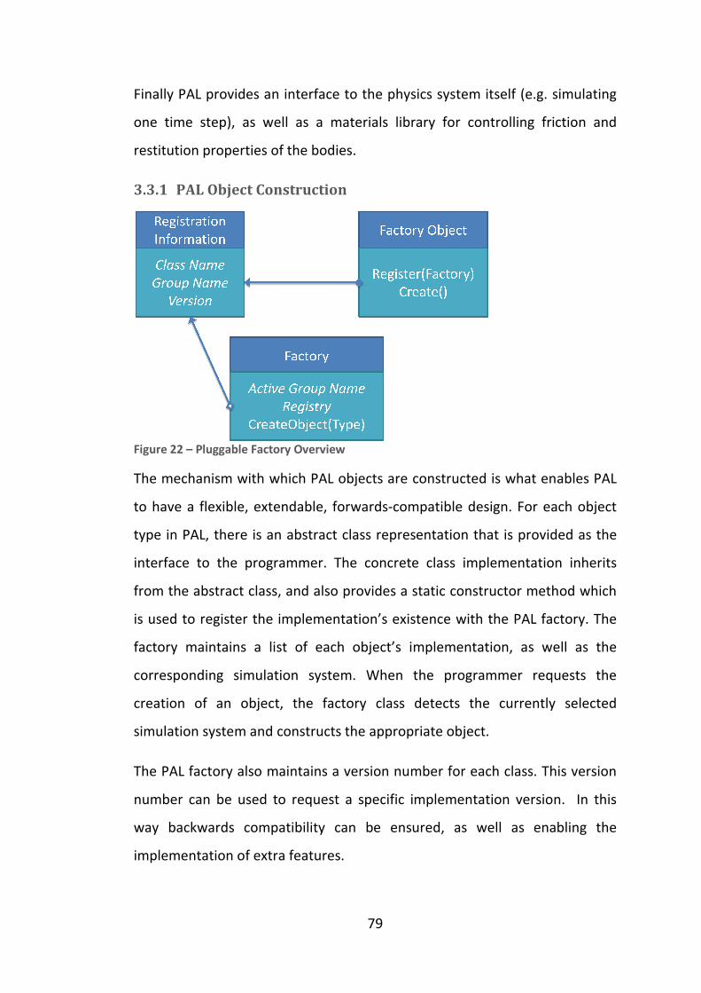
Finally PAL provides an interface to the physics system itself (e

one time step), as well as a materials library for controlling frictio

restitution properties of the bodies.

3.3.1 PAL Object Construction

Figure 22 – Pluggable Factory Overview

The mechanism with which PAL objects are constructed is what enables PAL

to have a flexible, extendable, forwards

type in PAL, there is an abstract class representation that is provided as the

interface to the programmer.

from the abstract class, and also provides a static constructor method which

is used to register the implementation’s existence with the PAL factory. The

factory maintains a list of each object’s implementation,

corresponding simulation system. When the programmer requests the

creation of an object, the factory class detects the currently selected

simulation system and constructs the appropriate object.

The PAL factory also maintains a version numbe

number can be used to request a specific implementation version. In this

way backwards compatibility can be ensured, as well as enabling the

implementation of extra features.

79

Finally PAL provides an interface to the physics system itself (e

one time step), as well as a materials library for controlling frictio

restitution properties of the bodies.

PAL Object Construction

Pluggable Factory Overview


to have a flexible, extendable, forwards-compatible design.

there is an abstract class representation that is provided as the

interface to the programmer. The concrete class implementation inherits



factory maintains a list of each object’s implementation,



simulation system and constructs the appropriate object.

The PAL factory also maintains a version number for each class. This version



implementation of extra features.

Finally PAL provides an interface to the physics system itself (e.g. simulating

one time step), as well as a materials library for controlling friction and


compatible design. For each object

there is an abstract class representation that is provided as the

concrete class implementation inherits



factory maintains a list of each object’s implementation, as well as the



r for each class. This version



80

For example, if we wish to create a sphere then we require a physics library

implementation of this. The physics library implementation would inherit

from the factory object, and provide functionality to create a copy of itself, as

well as the registration information. This includes the version of the

implementation, the name of the class (e.g. “sphere”), and the

implementation group it belongs to (e.g. “Bullet”). An alternative physics

library implementation would provide the same information, except a

different entry for the group (e.g. “ODE”).

When a programmer specifies the physics library they wish to use (e.g.

“Bullet”), the factory updates its registry to only include the highest version

entries for the given physics library. When the programmer creates a sphere,

the PAL factory searches through its registry to find a new entry that matches

this (e.g. “sphere”) and returns the appropriate object (e.g. a Bullet sphere).

3.3.2 PAL Geometries and Bodies

The physics abstraction layer requires a unique design to achieve its goals. To

maintain maximum compatibility, redundant implementations of similar

concepts are provided. For example, not all physics libraries provide a

distinction between a physical body, and a simple geometry. Thus, within PAL

there are two ways to represent a sphere. Once, as a PAL rigid body that

contains a sphere geometry, and once as a PAL sphere (a combined rigid

body/sphere representation). This way, if a physics engine provides

functionality for separate geometries, then when a PAL sphere is created, it

will default to attaching a sphere geometry to a body. If not, than the default

implementation is not invoked and the physics engine explicitly constructs a

spherical rigid body.

Figure 23 – PAL Sphere representation

There are a number of distinct cases to co

rigid bodies with a given geometry. The set of geometry types supported by

PAL is illustrated in

Figure 24 – PAL Geometry types

81

PAL Sphere representation

There are a number of distinct cases to consider for the representation of


PAL is illustrated in Figure 24.

PAL Geometry types

nsider for the representation of


82

Geometry support within a physics engine can be broadly broken down into

the following categories:

1. Geometry is fully supported, regardless of body type

2. Geometry is unsupported, regardless of body type

3. Geometry is supported, but only for static bodies

4. Geometry is supported, but only for static or kinematic bodies

5. Geometry is supported, but only for dynamic bodies

6. Geometry is unsupported, however other geometries can be used to

represent this type

The first two cases are straight-forward to support within PAL. If the

geometry type is completely supported, it is fully implemented in PAL’s

geometry class structure. If it is not supported, then it is ignored and PAL will

handle error cases.

In the third case, the geometry is supported by the physics engine, but only

for static (unmovable) bodies. This is a common case for many geometry

types, such as planes, heightmaps and concave meshes. Since it is a common

case, an alternative representation for the geometries are provided as

“terrain” representations. The terrain can represent heightmaps, polygon

meshes (concave geometries), and planes (orientated, or axis-aligned). These

types are illustrated in Figure 25. A separate distinction is made between axis

aligned planes, and planes which can have any orientation, in order to

provide maximum support for physics engines which do not provide an

orientated plane representation.

Figure 25 – PAL Terrain types

If a physics engine can only represent a terrain geometry as a static body,

then it is purely represented as a terrain. This helps avoid confusing the user

with having geometry types available that cannot be assigned to bodies.

Otherwise, the geometry representation is available, but can only be used for

creating static bodies. If the user attempts

body then PAL will return an error.

The fourth case (geometry supported by static and kinematic bodies) is

handled in a similar manner. The geometry has an implemented

representation within PAL, but returns an error when

with a dynamic body. The fifth case is the reciprocal of the fourth, where the

geometry will only support dynamic bodies, yet will not support static bodies.

In the sixth case the geometry is unsupported directly by the physics engine

however, it can be represented using alternative means. This broadly falls

into two common categories, depicted in

geometry type is not supported is a subset of a geometry type that is

supported. An examp

objects, but does not support the representation of a capsule. To handle this

PAL employs the template design pattern. PAL provides an abstract set of

83

PAL Terrain types


represented as a terrain. This helps avoid confusing the user



creating static bodies. If the user attempts to assign a geometry to a dynamic

body then PAL will return an error.



representation within PAL, but returns an error when the geometry is used



In the sixth case the geometry is unsupported directly by the physics engine


into two common categories, depicted in Figure 26. First, where the


supported. An example of this is a physics engine that supports convex




represented as a terrain. This helps avoid confusing the user



to assign a geometry to a dynamic



the geometry is used



In the sixth case the geometry is unsupported directly by the physics engine,


. First, where the


le of this is a physics engine that supports convex



methods for creating a geometry representation as a s

enabling the physics engine to construct the simpler geometry using the

convex geometry type.

Figure 26 – Alternative geometry representations. Left

Geometry composition

The other category is geometries that are not subsets of a supported

geometry, but can be estimated from the composition of an alternative. An

example of this is if a physics engine does not provide a plane representation,

but provides support for a static box inste

aggregation and special case code. This may not result in the geometry being

supported universally by the physics engine, rather just as a hard

terrain representation.

Since very few physics engines support dynamic bodies wit

geometry, an alternative rigid body type is provided that can contain multiple

simpler geometries. This enables complex geometry to be reconstructed

from compound simple geometries. Most physics engines support a

compound body type, however, few

adding or removing geometries to a body once they are created. This poses a

problem since some physics engines require the creation of a body and then

attaching geometries to it, whereas others require the geometries to

defined when the body is created.

84

methods for creating a geometry representation as a set of triangles,


Alternative geometry representations. Left – Geometry subsets, Right

category is geometries that are not subsets of a supported



but provides support for a static box instead. This is handled with


supported universally by the physics engine, rather just as a hard

Since very few physics engines support dynamic bodies with concave




compound body type, however, few physics engines support dynamically



attaching geometries to it, whereas others require the geometries to

defined when the body is created.

et of triangles,


Geometry subsets, Right –

category is geometries that are not subsets of a supported



ad. This is handled with


supported universally by the physics engine, rather just as a hard-coded

h concave




physics engines support dynamically



attaching geometries to it, whereas others require the geometries to be

85

This is achieved by using lazy evaluation. Each geometry is added to the body

is stored in a buffer and once the body is finalized all the geometries can be

processed within one call, regardless of how the underlying physics engine

requires the compound body to be constructed.

There are a number of additional separate rigid body types that may be

supported by a physics engine.

• Static bodies – Bodies that are not moveable, such as terrain. These

exist purely for collision detection.

• Kinematic bodies – Bodies that can be moved, but do not respond to

forces or collisions. These allow objects to move in predefined

motions and interact with the dynamic objects in the scene.

• Dynamic bodies – Bodies that respond to forces and collisions. The

movement of these bodies is calculated from the forces applied to the

body.

• Compound bodies – Bodies that contain multiple geometries.

PAL provides one additional body type:

• Generic body – This is a body that can be switched between all

representations and can have geometries dynamically added and

removed.

Physics engines do not implement the various body types according to these

strict definitions. The physics engines that do conform to this are directly

implemented in PAL. Physics engines that do not support a certain body type

do not have that body type implemented. There is no attempt to emulate

higher level functionality with the use of other bodies.

Figure 27 – PAL Body types

Emulating additional functiona

example, if a static or kinematic body is emulated with a dynamic body then

all forces acting on the body would have to be negated. That is, if gravity is

being applied to a body, a force would have to be appli

magnitude in the opposite direction in which gravity is acting. Over time

numerical differences between the set position of the body and the position

attempting to be maintained start diverging and the body will begin to drift.

Some physics engines provide partial implementations of a body type.

Physics engines will often provide the ability to reposition static bodies,

enabling some of the functionality of a kinematic body to be achieved.

However, this movement does not influence any bodie

between the static bodies starting position and ending position. As a result

the static body may overlap or entirely contain a dynamic body, leading to

unstable results. To avoid these instabilities this functionality is not

supported in PAL.

86

Emulating additional functionality will often lead to unstable results. For



being applied to a body, a force would have to be applied of the same




s engines provide partial implementations of a body type.



However, this movement does not influence any bodies that lie on the path




lity will often lead to unstable results. For



ed of the same




s engines provide partial implementations of a body type.



s that lie on the path




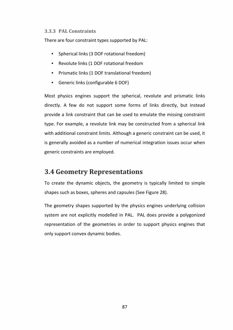
87

3.3.3 PAL Constraints

There are four constraint types supported by PAL:

• Spherical links (3 DOF rotational freedom)

• Revolute links (1 DOF rotational freedom

• Prismatic links (1 DOF translational freedom)

• Generic links (configurable 6 DOF)

Most physics engines support the spherical, revolute and prismatic links

directly. A few do not support some forms of links directly, but instead

provide a link constraint that can be used to emulate the missing constraint

type. For example, a revolute link may be constructed from a spherical link

with additional constraint limits. Although a generic constraint can be used, it

is generally avoided as a number of numerical integration issues occur when

generic constraints are employed.

3.4 Geometry Representations

To create the dynamic objects, the geometry is typically limited to simple

shapes such as boxes, spheres and capsules (See Figure 28).

The geometry shapes supported by the physics engines underlying collision

system are not explicitly modelled in PAL. PAL does provide a polygonized

representation of the geometries in order to support physics engines that

only support convex dynamic bodies.

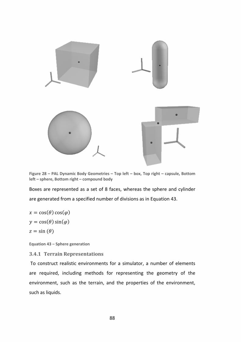
Figure 28 – PAL Dynamic Body Geometries

left – sphere, Bottom right – compound body

Boxes are represented as a set of 8 faces, whereas the sphere and cylinder

are generated from a specified numb

= cos( cos( n = cos( sin( = sin (

Equation 43 – Sphere generation

3.4.1 Terrain Representations

To construct realistic environments for a simulator, a number of elements

are required, including methods for representing the geometry of the

environment, such as the terrain, and the properties of the environment,

such as liquids.

88

PAL Dynamic Body Geometries – Top left – box, Top right – capsule, Bottom

compound body


are generated from a specified number of divisions as in Equation 43

Sphere generation

Terrain Representations




capsule, Bottom


43.




89

All robotic systems, with the exception of space robots, have some form of

immobile environment with which they interact. Depending on the

configuration a number of different environment terrain models are

applicable. For example, when simulating a robot in a laboratory it may be

appropriate to approximate the environment as a simple plane. Alternatively,

the simulation of an automobile would require a more detailed

representation of the environment, such as a height map.

A plane is the simplest type of environment a robotic system can be found in.

It represents a perfectly flat surface. The equation of a plane is given by:

# + Bn + a + = 0

Equation 44 – Equation of a plane

Where (a,b,c) is the normal of the plane. To determine the equation of a

plane given a normal vector and a point the parameter d can be calculated

from:

= −51.

Where 51 is the plane normal

p is a point on the plane Equation 45 – Plane Equation

Any larger representations of a more complex terrain can be locally

represented as a plane. In order to achieve this representation three points

(i.e. vertices) are required on the complex terrain to construct a plane

representation. All that is required is to calculate the plane’s normal, as the

rest can be calculated from Equation 45.

51 = (y9 − yu × (y − yu

Where 51 is the plane normal

and p1,p2,p3 are three points from the complex terrain. Equation 46 – Normal from three points

90

The plane model is required in PAL such that PAL can convert between

different representations (e.g. point and normal form) and construct the

appropriate position matrix for representing a plane with a box.

To create a representation of the plane with a box, the orientation, position,

and dimensions of the box are required. The size of the box can be

determined from the size of the simulated world.

The position of the box on an infinite plane is arbitrary – it can be anywhere

on the plane. The best choice is typically the closest point on the plane to

the origin of the world as this will allow the size of the box to match the

world size (which is typically constrained within a virtual box). The closest

point on the plane to the origin can be determined from the Euclidian

distance to the origin constrained on the plane. This is given in Equation 47.

, n, = ##9 + B9 + a9 , B#9 + B9 + a9 , a#9 + B9 + a9

Equation 47 – Point on plane closest to origin

A rotation matrix for an object is constructed from three basis vectors. These

three vectors are orthogonal from one another. Given the normal of a plane,

the two other basis vectors required can be generated by providing initial

estimates for the basis vectors and enforcing they are orthonormal. The

process for this is:

• Estimate basis vectors as [0,0,1] [0,1,0], [1,0,0].

• Perform a dot-product with the estimated basis vectors and the plane

normal

• Select the lowest dot-product as the best-estimate tangent to the

normal. (The dot product between two perpendicular vectors is zero)

• Create the vector perpendicular to both the estimated tangent and

the normal via the cross product. (i.e. bi-tangent)

91

• Create true orthogonal vectors with the true normal and estimated

tangent and bi-tangent via orthogonalization (e.g. Gram–Schmidt

process)

Given the rotation matrix, position and dimensions required the plane can

then be reconstructed and modelled with a large box instead.

Heightmaps are a 2-D domain, containing a displacement at each point from

the origin of a surface (See Figure 29). This representation is advantageous

as it is compact and is commonly used in geographic information systems

allowing for digital elevation models to be used within a simulator.

Figure 29 - Heightmap

PAL requires an internal model of the heightmap terrain, as some physics

engines do not support this type. Nevertheless, it can be implemented if a

more general polygon soup mesh is available. Heightmaps are triangulated

by processing four adjacent data points at a time, first constructing a triangle

from the top left set, then the bottom right set. (See Figure 30)

Figure 30 – Left - Triangulated height data, Right

The most versatile representation is a generalized polygon mesh

representation. It allows concave object representations and is extremely

useful for modelling the terrain. This allows for the simulation of indoor

environments, as well as more complex outdoors scenes. Height

subset of a terrain mesh, allowing a terrain mesh to augment a scene

described by a geographic information system

format is natively supported by the physics engine’s collision detection

system, and so there is no m

itself.

3.5 Fluid Model Representations


physics are the fluid effects. These are mostly the drag and lift effects, and

the buoyancy forces. These can either be modelled and applied directly to

the bodies, or the behaviour of the liquid itself can be modelled and then

applied to the bodies.

Directly modelling the liquid forces that are applied to the bodies has the

advantage of being less comp

techniques. Many of the forces can be experimentally verified, providing a

good model of global effects on a body. The interaction of liquid between

92

Triangulated height data, Right – Two step triangulation

representation is a generalized polygon mesh



environments, as well as more complex outdoors scenes. Heightmaps are a


geographic information system digital elevation model. This


system, and so there is no model for a generalized polygon soup within PAL

Fluid Model Representations



These can either be modelled and applied directly to



advantage of being less computationally intensive than liquid modelling



representation is a generalized polygon mesh



maps are a


digital elevation model. This


odel for a generalized polygon soup within PAL



These can either be modelled and applied directly to



utationally intensive than liquid modelling



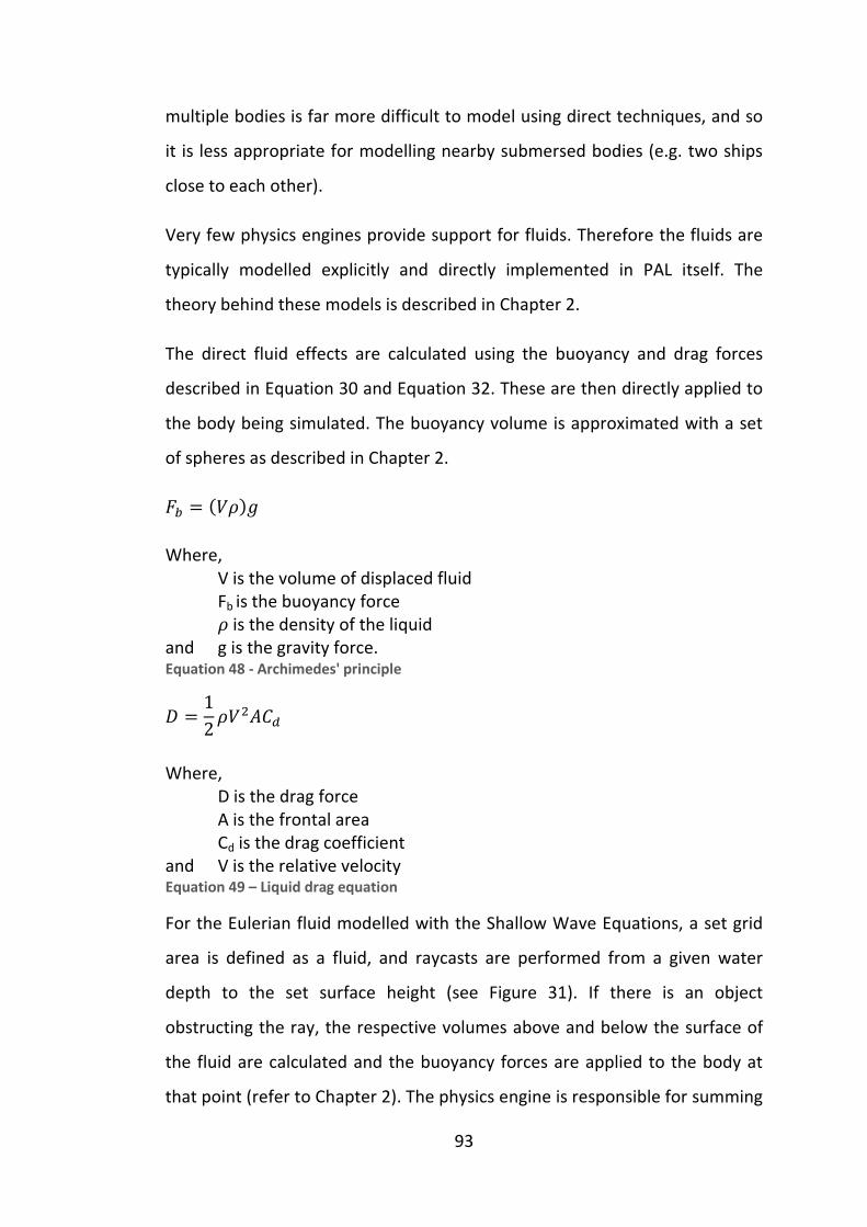
93

multiple bodies is far more difficult to model using direct techniques, and so

it is less appropriate for modelling nearby submersed bodies (e.g. two ships

close to each other).

Very few physics engines provide support for fluids. Therefore the fluids are

typically modelled explicitly and directly implemented in PAL itself. The

theory behind these models is described in Chapter 2.

The direct fluid effects are calculated using the buoyancy and drag forces

described in Equation 30 and Equation 32. These are then directly applied to

the body being simulated. The buoyancy volume is approximated with a set

of spheres as described in Chapter 2.

M = (VWX

Where,

V is the volume of displaced fluid

Fb is the buoyancy force

W is the density of the liquid

and g is the gravity force. Equation 48 - Archimedes' principle

\ = 12 WV9?-

Where,

D is the drag force

A is the frontal area

Cd is the drag coefficient

and V is the relative velocity Equation 49 – Liquid drag equation

For the Eulerian fluid modelled with the Shallow Wave Equations, a set grid

area is defined as a fluid, and raycasts are performed from a given water

depth to the set surface height (see Figure 31). If there is an object

obstructing the ray, the respective volumes above and below the surface of

the fluid are calculated and the buoyancy forces are applied to the body at

that point (refer to Chapter 2). The physics engine is responsible for summing

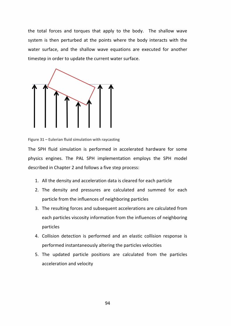
94

the total forces and torques that apply to the body. The shallow wave

system is then perturbed at the points where the body interacts with the

water surface, and the shallow wave equations are executed for another

timestep in order to update the current water surface.

Figure 31 – Eulerian fluid simulation with raycasting

The SPH fluid simulation is performed in accelerated hardware for some

physics engines. The PAL SPH implementation employs the SPH model

described in Chapter 2 and follows a five step process:

1. All the density and acceleration data is cleared for each particle

2. The density and pressures are calculated and summed for each

particle from the influences of neighboring particles

3. The resulting forces and subsequent accelerations are calculated from

each particles viscosity information from the influences of neighboring

particles

4. Collision detection is performed and an elastic collision response is

performed instantaneously altering the particles velocities

5. The updated particle positions are calculated from the particles

acceleration and velocity

95

This process is repeated every timestep to update the fluid state. The

smoothing kernels used are given in Equation 50, Equation 51, and Equation

52.

31564Yℎ (ℎ9 − [9

Equation 50 – The SPH density smoothing kernel (poly6)

− 45Yℎ (ℎ − [9

Equation 51 – The SPH pressure smoothing kernel (spiky)

45Yℎ (ℎ − [

Equation 52 – The SPH viscosity smoothing kernel

3.6 Actuator Models

Accurate modelling of actuator behaviour is critical for simulating realistic

motions. To simulate an actuator a number of models are required to

produce the final desired behaviour.

3.6.1 Generic Angular Velocity Motor Model

A simple angular velocity motor can be simulated by applying impulses to

two bodies connected by a revolute joint. The current axis of the joint can be

calculated using the transformation matrix of the parent body:

a#311111111111 = " #311111111 3ym11111111111111111 = a#311111111111 ∗ [5Xℎ

Where, M is the parents rotation matrix

#311111111 is the original joint axis

a#311111111111 is the current joint axis

strength is the scalar strength of the impulse being applied

and 3ym11111111111111111 is the impulse applied to the parent body Equation 53 – Impulse model for a angular velocity motor

96

The impulse is then applied to the parent body and a negative impulse is

applied to the child body.

3.6.2 Generic Angular Position Motor Model

To simulate a generic angular position motor model a standard Proportional-

Integral-Derivative (PID) controller is coupled to the angular velocity motor

model (See Section 5.1.1 on PID control). The input error to the PID

controller is the difference between the joints current angle and the desired

angle (wrapped between 0 and 2π), and the time since the last update (i.e.:

the integrator step size). The output value from the PID controller is then

applied to the underlying angular velocity motor model.

3.6.3 DC Motor Model

The DC motor torque can be mathematically modelled using the standard

armature controlled DC motor model (91), represented by:

K( = + VK( − M=( K

Where, Ra is the Armature resistance (ohms)

KT is the motor torque constant (Nm/A)

Kb is the motor back EMF constant (Vs/rad)

ωn is the angular velocity of motor (rad/s)

and Va is the applied armature voltage (Volts) Equation 54 - Armature Controlled DC Motor Torque Equation (91)

The armature model can also be described as a transfer function for the

motor in terms of an input voltage (V) and output rotational speed (θ):

V = (* + B( + + 9

Where, J is the moment of inertia of the rotor,

b is the damping ratio of the mechanical system,

L is the rotor electrical inductance,

R is the terminal electrical resistance,

and K is the electro motive force constant. Equation 55 - Armature controlled DC motor model transfer function (91)

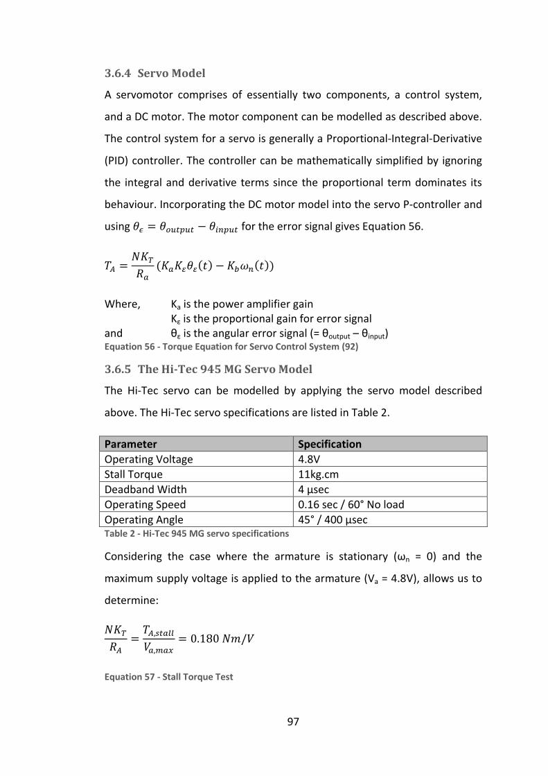
97

3.6.4 Servo Model

A servomotor comprises of essentially two components, a control system,

and a DC motor. The motor component can be modelled as described above.

The control system for a servo is generally a Proportional-Integral-Derivative

(PID) controller. The controller can be mathematically simplified by ignoring

the integral and derivative terms since the proportional term dominates its

behaviour. Incorporating the DC motor model into the servo P-controller and

using = Ux(x( − T=x( for the error signal gives Equation 56.

= + K (K( − M=(

Where, Ka is the power amplifier gain

Kε is the proportional gain for error signal

and θε is the angular error signal (= θoutput – θinput) Equation 56 - Torque Equation for Servo Control System (92)

3.6.5 The Hi-Tec 945 MG Servo Model

The Hi-Tec servo can be modelled by applying the servo model described

above. The Hi-Tec servo specifications are listed in Table 2.

Parameter Specification

Operating Voltage 4.8V

Stall Torque 11kg.cm

Deadband Width 4 µsec

Operating Speed 0.16 sec / 60° No load

Operating Angle 45° / 400 µsec Table 2 - Hi-Tec 945 MG servo specifications

Considering the case where the armature is stationary (ωn = 0) and the

maximum supply voltage is applied to the armature (Va = 4.8V), allows us to

determine:

+ = ,(K^^VK,K' = 0.180 /V

Equation 57 - Stall Torque Test

98

When the motor is at top speed, the applied armature voltage equals the

back EMF, i.e. VK( = &=,K'(. From the servo specifications the

maximum angular velocity is known, so the motor back EMF constant can be

calculated:

& = VK,K'=,K' = 0.733 V/[#

Equation 58 - Maximum Speed Test

This gives:

= 0.180(VK( − 0.733=(

Equation 59 - Servo Torque Equation

The proportional component of the controller was modelled with Equation

60. The model assumes that the maximum supply voltage is applied to the

motor, until its gets within a tolerance of the desired angle. The voltage

applied to the motor is then linearly decreased, until the servo reaches its

final destination.

VK = (, ( < VK,K'VK,K', ℎ[4 Equation 60 - Armature Voltage P-Controller Model

This model performed adequately for large movements, however it was

found that for small angle movements, where the maximum armature

voltage was not achieved, the servo model was not accurate since the full

stall torque is not applied. To overcome this, it is assumed that the maximum

supply voltage is always applied to the armature. This is a reasonable

assumption, since the slowing down of the servo has only a minor effect on

its time response.

The deadband specification of the servo was used to decide when the servo

model had reached its target angle. Once the servo is deemed to have

99

reached its destination, a torque is no longer applied to the joint. This is

shown in Equation 61.

= 0, %x&=( − (K &( < &KMK=2, ℎ[4 Equation 61 - Servo Deadband Model

3.6.6 Thruster Model

The default thruster model implemented is based on the lumped parameter

dynamic thruster model developed by D. R. Yoerger et al. (59). The thrust

produced is governed by:

ℎ[m = -(Ω|Ω| Where Ω is the propeller angular velocity,

and Ct is the proportionality constant.

Equation 62 – Lumped parameter dynamic thruster model

3.6.7 Control Surfaces

Control surfaces are movable surfaces that affect the movement of a body in

a fluid. Control surfaces are typically found on aircraft (e.g. ailerons), ships

(e.g. rudders) and underwater vehicles (e.g. fins). The model used to

determine the lift from diametrically opposite fins (61) is given by:

ST= = 12 W-_¢S£ST=¤&&9

Where,Lfin is the lift force,

ρ is the density,

CLδf is the rate of change of lift coefficient with respect to fin effective

angle of attack,

Sfin is the fin platform area,

δe is the effective fin angle, &is the effective fin velocity Equation 63 – Fin control surface lift model

100

3.7 Sensor Models

The Physics Abstraction Layer can simulate a number of sensors. Each sensor

can be coupled with an error model to allow the simulation of sensor data

similar to the accuracy of the physical equipment that is being simulated.

Many of the positional and orientation sensors can be directly modelled from

the data available from the lower level physics library. Every sensor is

attached to a body that represents a physical component of a robot.

3.7.1 Inclinometer

The simulated inclinometer sensor calculates its orientation from the

orientation of the body that it is attached to, relative to the inclinometer’s

own initial orientation. Given a normalized vector indicating the forward axis

of the inclinometer, fwd and the body’s current 3x3 rotation matrix M we can

calculate the new rotated forward axis vector rfwd:

[$11111111111 = " $11111111

Equation 64 – Axis transformation

The angle between these two vectors can be calculated as:

θ = cosLu[$11111111111. $11111111 Equation 65 – Angle between two vectors

This provides only a positive angle, and does not indicate a difference

between the vector being “in front of” or “behind” the vector. This can be

calculated by creating a virtual “right” vector, indicating a vector

perpendicular to the front vector. This vector can be generated from the

forward axis and a 3x3 rotation matrix R, representing a 90 degree rotation.

[3Xℎ11111111111 = $11111111

Equation 66 – Right vector transformation

101

Then following a similar procedure to find the angle between the right axis

and the forward axis:

[[3Xℎ1111111111111 = " [3Xℎ11111111111

= [[3Xℎ1111111111111 . $11111111

Equation 67 – Angle sign calculation

If the dot product is less than zero, the angle becomes negative.

3.7.2 Gyroscope

Similarly to the inclinometer, the simulated gyroscope calculates its

orientation from the attached body’s angular velocity, and its own axis of

rotation. In the case of the engine being able to directly provide the bodies

angular velocity, the calculation simply becomes a dot product between the

angular velocity (ω) and the gyroscopes axis:

= #311111111. 11

Equation 68 – Gyroscope angle calculation

3.7.3 Velocimeter

The velocimeter calculates the velocity in a given direction from its

orientation axis and the velocity information from the attached body. Again,

given the physics engines ability to directly provide a body’s linear velocity,

the calculation is a dot product between the linear velocity (v) and the

velocimeters axis:

= #311111111. Equation 69 – Scalar velocity calculation

3.7.4 PSD Sensor

Distance measuring sensors, such as echo-sounders and Positional Sensitive

Devices (PSDs) are simulated by traditional ray casting techniques, provided

the low level physics library supports the necessary data structures and ray

102

casting routines. The implementation of the PSD sensor depends highly on

the ray casting functionality provided by the physics engine (if it is provided

at all). Otherwise the ray cast routine is dependent on the spatial partitioning

data structures employed by the low-level physics library. If the physics

library directly provides a routine for raycasting given an axis and a starting

point, then this information can be directly pass to it by PAL. If the engine

requires the start and end points for the ray, then this can be calculated

from:

¦§¨©§ = "ª

Where, start is the ray start point

M is the body’s rotation matrix

and o is the original start points offset relative to the body’s position Equation 70 – Point transformation

The end point can then be calculated by finding the direction of the axis

©¨ = "# 5#1111 = «©¨ − « ¬® = ¦§¨©§ + 5#1111 ∗ [#5X

Where, end is the ray end point

start is the ray start point

M is the body’s rotation matrix

# is the axis indicating the direction of the PSD

ra is the rotated axis position

p is the position of the body

and range is the distance the PSD can sense. Equation 71 – Ray end point calculation

3.7.5 GPS

A rudimentary GPS sensor can be simulated given certain assumptions, such

as that the simulation takes place within a narrow range of the earth’s

latitude. The GPS position can be calculated from Equation 72.

103

# = y. y ∗ 3600

5X = y. y ∗ 3600 #"45 = $[#a([2(# ∗ 60

5X"45 = $[#a([2(5X ∗ 60

Where , p is the bodies position

Mps is the meters per arc second of the earth at the current

earths latitude

lat is the latitude in arc seconds

long is the longitude in arc seconds

latMin is the latitude in arc minutes

and longMin is the longitude in arc minutes Equation 72 – GPS latitude and longitude calculation

The checksum can be calculated as follows:

int i=0; int checksum=0; while (buffer[i]!= '*' ) checksum^=buffer[i]; i++;

Listing 2 – GPS Checksum calculation

3.7.6 Contact Sensor

Contact sensors are simulated by querying the collision detection routines of

the low-level physics library for the positions where collisions occurred. If the

collisions queried occur within the domain of the contact sensors, then these

collisions are recorded. The mechanics involved with detecting, storing and

sorting the relevant collision information are highly dependent on each

physics library’s implementation. Typically this involves inspecting the physics

engine’s collision subsystem and creating a callback function to store and

sort all the contact information. Contact generation is an extremely complex

task that has a large influence on the stability and robustness of the physics

engine.

104

4 Physics Engine Evaluation

In the past it has been very difficult to compare physics engines, however

recently a number of physics engine abstraction systems have become

available such as PAL (Physics Abstraction Layer) (93), which was developed

for this thesis, OPAL (Open Physics Abstraction Layer) (69), and

GangstaWrapper (72). These abstraction layers allow developers to

implement one version of their physics system through a unique interface

and test their application with multiple engines before constructing a final

release. Additionally, they simplify the task of comparing physics engines

directly.

The Open Physics Abstraction Layer is the least complete, providing only an

interface to one physics engine. The GangstaWrapper provides an interface

to four physics engines, whereas PAL provides support for more than ten

engines. GangstaWrapper is no longer maintained, however provides a solid

interface for the physics engines it supports.

An alternative approach to achieving physics engine interoperability is the

COLLADA (70) standard. Coumans and Victor (71) provide a brief overview

article of the COLLADA physics standard and provide a short comparison of

the capabilities of the Bullet (79), Novodex (Ageia/nVidia PhysX) (78) , ODE

(Open Dynamics Engine) (86) and Havok (81) physics engines.

Seugling and Rolin (94) published an article comparing three different physics

engines, Newton (84), Novodex (Ageia/nVidia PhysX), and ODE (Open

Dynamics Engine). Their evaluation focused primarily on the performance of

the systems for simulators. In this Chapter similar tests will be conducted and

analysed with an additional focus on real-time capable technology. From

their test results they concluded that Novodex (Ageia PhysX) provided the

best results. Although most of the tests provided a quantitative difference in

105

performance, the final evaluation was determined from a very rough grading

system. As a result the final findings did not necessarily reflect significant

performance differences in the individual tests between physics engines.

Most physics engines have a particular target application to which they are

optimized. This results in different performance in each and extra features

are often made available specifically for a target application. PAL supports

more than ten different physics engines, of which seven are tested in this

comparison. The engines supported by PAL are nVidia/AGEIA PhysX(78) (also

referred to as Novodex), Bullet Physics Library (79), Dynamechs (80), Havok

(81), IBDS (82), JigLib (83), Meqon (85), Newton Physics SDK (84), Open

Dynamics Engine (86), OpenTissue Library (87), Tokamak (89), True Axis

Physics SDK (90).

There are five engines supported by PAL that are not tested. Dynamechs is

not tested, as it does not support collisions between two dynamic bodies. It

only supports collisions between dynamic and static bodies. Meqon is not

tested, as it is no longer distributed, and the OpenTissue Library was not

included since it is not a complete physics engine, rather a meta-library and

thus it is difficult to construct a fair and general test configuration. Havok and

IBDS were not examined as PAL does not have a complete implementation of

the physics engines’ capabilities.

4.1 Physics Engine Evaluation Tests

Five tests were performed to assess the aspects of the physics engines. These

are integrator, material, constraint, collision and stacking tests. 2

2 Note: A video of these tests is available from the Eurographics 2007 physics stream

http://isg.cs.tcd.ie/eg07/, or on youtube: http://www.youtube.com/watch?v=IhOKGBd-7iw

The source code for these tests is available from the CVS repository of the PAL project at

http://pal.sourceforge.net/

106

4.1.1 Integrator Performance

Figure 32 – Integrator test configuration

The integrator is responsible for calculating a body’s position given the forces

acting on it. The performance of the integrator affects the accuracy of the

simulation. To test the integrator a very simple test is performed. A sphere is

constructed at the origin and allowed to drop from gravitational forces.

Gravity is set to -9.8m/s, and the time step is set to 0.01s. The positions

presented by the physics engines are then recorded and compared to ideal

cases for various integrators. From classical physics, the position of a body

with no initial velocity can be calculated from:

[ = 12 #9

Where [ is the body’s displacement

# is the body’s acceleration

and is time. Equation 73 – Uniform acceleration

107

Figure 33 – Positional error from cumulative numerical integrators relative to the ideal

case normalized to the Symplectic Euler integrator error

Figure 33 illustrates the accumulated position errors due to the integrator

relative to the ideal case presented above. The errors have been normalized

with respect to the Symplectic Euler integrator. Most physics engines provide

results similar to the Symplectic Euler integrator, or 2nd

order Euler. Novodex

(Ageia PhysX) provided the best results. The integrator for the Newton

physics engine provided the worst results, with over 40 times the relative

error of the Symplectic Euler integrator. For this reason it is not illustrated in

Figure 33. The Newton engine results were close to what would be expected,

if the physics system was simulating air drag of an extremely smooth object

(e.g. an aircraft wing (95)) However, this effect is due to forced velocity

dampening by the Newton integrator.

0

0.2

0.4

0.6

0.8

1

Normalized Relative Error Integrators Physics Engines

108

4.1.2 Material Properties

Figure 34 – Restitution test configuration

Materials are responsible for simulating friction and restitution properties

during a collision. Accurate friction and restitution models are critical for

simulation systems involving the interaction between two bodies (e.g.

walking robots).

The materials restitution properties were tested by colliding a box with a

sphere. The box is placed on the ground and the sphere is placed one meter

above. The box was of dimensions 1×1×1m3, and a mass of 1kg, the sphere

had a radius of 0.5m, and a mass of 1kg. Three different values of restitution

were tested, 0.1, 0.5 and 0.9. Since the box on the ground is stationary the

relationship between the dropped height and the coefficient of restitution is

given in classical physics by Equation 74.

109

-¯ = °ℎ±

Where -¯ is the coefficient of restitution

h is the bounce height

and ± is the drop height. Equation 74 – Coefficient of restitution

A graph of the bouncing boxes positioned over time for a restitution

coefficient of 0.5 is depicted in Figure 35. The maximum heights obtained

for the three different restitution values are given in Figure 36.

Figure 35 - Bounce height for a coefficient of restitution of 0.5

For course applications an accurate restitution model is unnecessary, more

important is that there is a correlation between an increase in restitution

value and the bounce height. Bullet and True Axis give acceptable relative

increases in the bounce height, and to a lesser extent Novodex, Newton and

Tokamak showed a correlation.

The level (e.g. position, velocity) at which a constraint based simulation

attempts to satisfy its constraints may cause drift due to numerical

-0.15

-0.1

-0.05

0

0.05

0.1

0.15

0.2

0.25

0.3

0.35

He

igh

t

Time

Height for Restitution = 0.5

Bullet

Jiggle

Newton

Novodex

ODE

Tokamak

TrueAxis

Ideal Max.

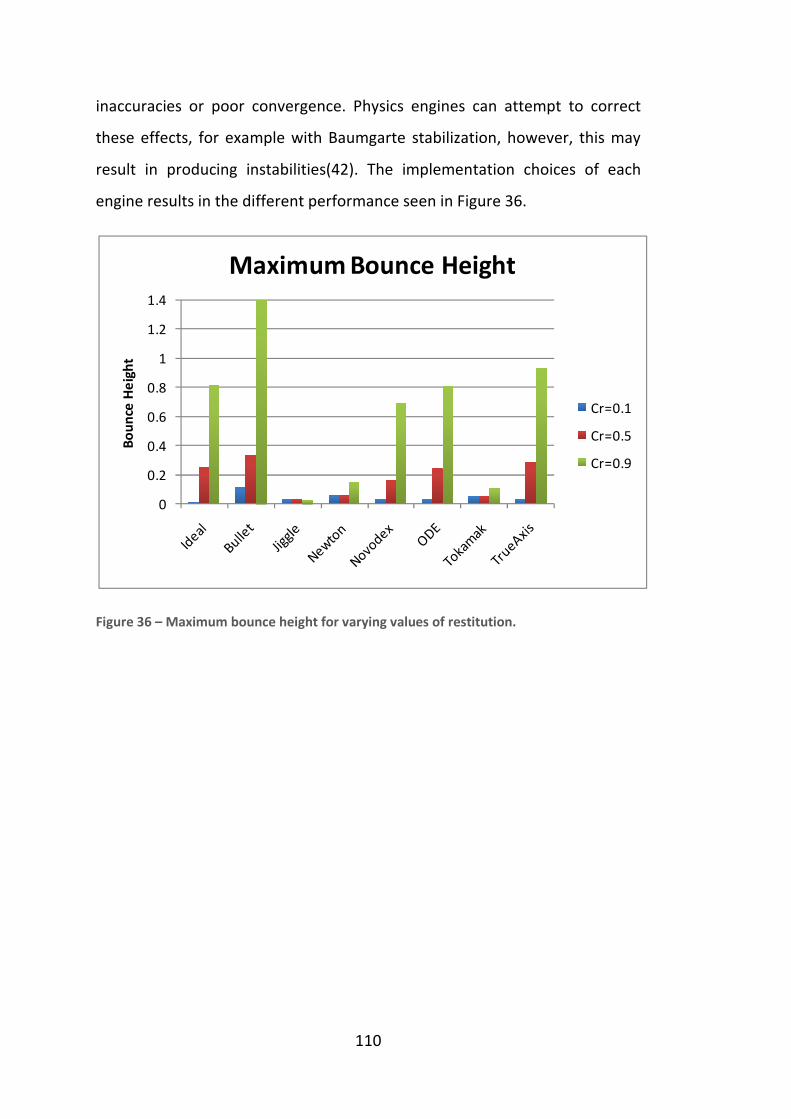
110

inaccuracies or poor convergence. Physics engines can attempt to correct

these effects, for example with Baumgarte stabilization, however, this may

result in producing instabilities(42). The implementation choices of each

engine results in the different performance seen in Figure 36.

Figure 36 – Maximum bounce height for varying values of restitution.

0

0.2

0.4

0.6

0.8

1

1.2

1.4

Bo

un

ce H

eig

ht

Maximum Bounce Height

Cr=0.1

Cr=0.5

Cr=0.9

111

Figure 37 - Friction test configuration

To test the static friction, a 5×1×5m box was placed on an inclined plane. A

static friction coefficient was assigned to the materials of the box and the

plane, and the angle of the plane was then incrementally increased to test

the angle at which the box would first start sliding. This process was repeated

for the range of static coefficients from 0.1 to 0.7, increasing by 0.1. The

angle of the plane was tested in the range of 0 to 0.7 in increments of 0.05

radians.

The Jiglib physics engine was not included in this test, as the PAL

implementation does not support resetting a body’s orientation after

construction.

The Newton physics engine provides the closest approximation of the ideal

results, with ODE providing the second best. Novodex also provides a good

approximation, however it applies too much static friction effect. All engines

display an increase in the angle required before motion occurs, indicating

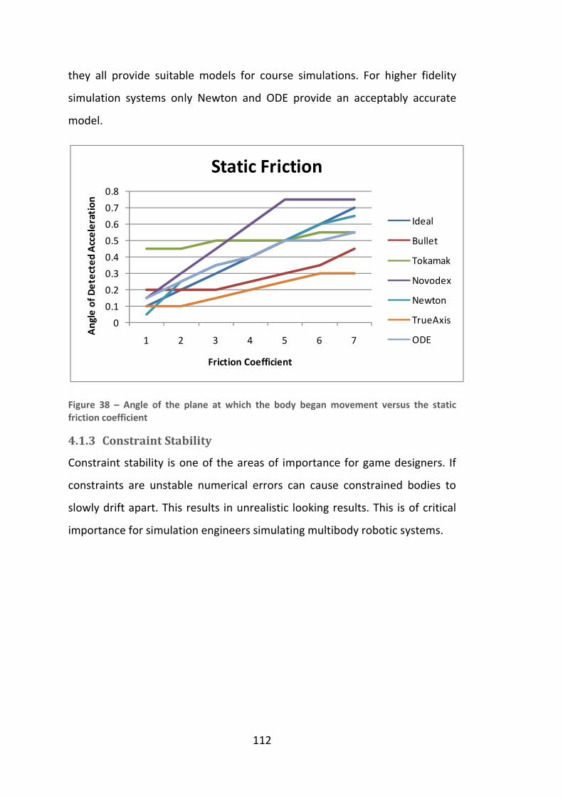
112

they all provide suitable models for course simulations. For higher fidelity

simulation systems only Newton and ODE provide an acceptably accurate

model.

Figure 38 – Angle of the plane at which the body began movement versus the static

friction coefficient

4.1.3 Constraint Stability

Constraint stability is one of the areas of importance for game designers. If

constraints are unstable numerical errors can cause constrained bodies to

slowly drift apart. This results in unrealistic looking results. This is of critical

importance for simulation engineers simulating multibody robotic systems.

0

0.1

0.2

0.3

0.4

0.5

0.6

0.7

0.8

1 2 3 4 5 6 7

An

gle

of

De

tect

ed

Acc

ele

rati

on

Friction Coefficient

Static Friction

Ideal

Bullet

Tokamak

Novodex

Newton

TrueAxis

ODE

113

Figure 39 – Constraint test configuration

To test the constraints’ stability, a chain of spherical links connecting a

number of spheres was simulated. The chain was attached to two boxes as

indicated in Figure 39. Each sphere in the chain had a radius of 0.2m, and a

mass of 0.1kg. The mass of the boxes was 400 times the number of

constraints.

The two side boxes were as high as the number of constraints, and the

supporting base measured 1x1m². The test was run for 20 seconds.

Figure 40 illustrates the constraint error measured from the accumulated

difference in the distance between two links from the initial distance. The

Newton physics engine is not illustrated as it contains significantly greater

error than other physics engines, averaging 30 times the error of other

engines.

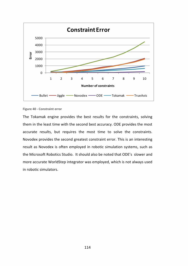
114

Figure 40 - Constraint error

The Tokamak engine provides the best results for the constraints, solving

them in the least time with the second best accuracy. ODE provides the most

accurate results, but requires the most time to solve the constraints.

Novodex provides the second greatest constraint error. This is an interesting

result as Novodex is often employed in robotic simulation systems, such as

the Microsoft Robotics Studio. It should also be noted that ODE’s slower and

more accurate WorldStep integrator was employed, which is not always used

in robotic simulators.

0

1000

2000

3000

4000

5000

1 2 3 4 5 6 7 8 9 10

Err

or

Number of constraints

Constraint Error

Bullet Jiggle Novodex ODE Tokamak TrueAxis

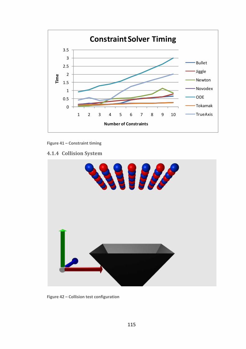
115

Figure 41 – Constraint timing

4.1.4 Collision System

Figure 42 – Collision test configuration

0

0.5

1

1.5

2

2.5

3

3.5

1 2 3 4 5 6 7 8 9 10

Tim

e

Number of Constraints

Constraint Solver Timing

Bullet

Jiggle

Newton

Novodex

ODE

Tokamak

TrueAxis

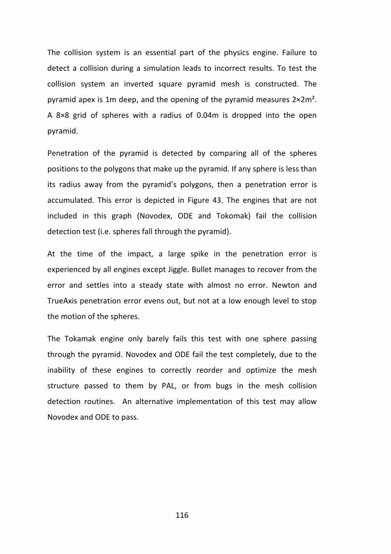
116

The collision system is an essential part of the physics engine. Failure to

detect a collision during a simulation leads to incorrect results. To test the

collision system an inverted square pyramid mesh is constructed. The

pyramid apex is 1m deep, and the opening of the pyramid measures 2×2m².

A 8×8 grid of spheres with a radius of 0.04m is dropped into the open

pyramid.

Penetration of the pyramid is detected by comparing all of the spheres

positions to the polygons that make up the pyramid. If any sphere is less than

its radius away from the pyramid’s polygons, then a penetration error is

accumulated. This error is depicted in Figure 43. The engines that are not

included in this graph (Novodex, ODE and Tokomak) fail the collision

detection test (i.e. spheres fall through the pyramid).

At the time of the impact, a large spike in the penetration error is

experienced by all engines except Jiggle. Bullet manages to recover from the

error and settles into a steady state with almost no error. Newton and

TrueAxis penetration error evens out, but not at a low enough level to stop

the motion of the spheres.

The Tokamak engine only barely fails this test with one sphere passing

through the pyramid. Novodex and ODE fail the test completely, due to the

inability of these engines to correctly reorder and optimize the mesh

structure passed to them by PAL, or from bugs in the mesh collision

detection routines. An alternative implementation of this test may allow

Novodex and ODE to pass.

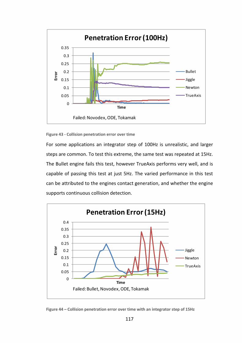
117

Figure 43 - Collision penetration error over time

For some applications an integrator step of 100Hz is unrealistic, and larger

steps are common. To test this extreme, the same test was repeated at 15Hz.

The Bullet engine fails this test, however TrueAxis performs very well, and is

capable of passing this test at just 5Hz. The varied performance in this test

can be attributed to the engines contact generation, and whether the engine

supports continuous collision detection.

Figure 44 – Collision penetration error over time with an integrator step of 15Hz

0

0.05

0.1

0.15

0.2

0.25

0.3

0.35

Err

or

Time

Penetration Error (100Hz)

Bullet

Jiggle

Newton

TrueAxis

Failed: Novodex, ODE, Tokamak

0

0.05

0.1

0.15

0.2

0.25

0.3

0.35

0.4

Err

or

Time

Penetration Error (15Hz)

Jiggle

Newton

TrueAxis

Failed: Bullet, Novodex, ODE, Tokamak

118

4.1.5 Stacking

Figure 45 - Box stacking test configurations

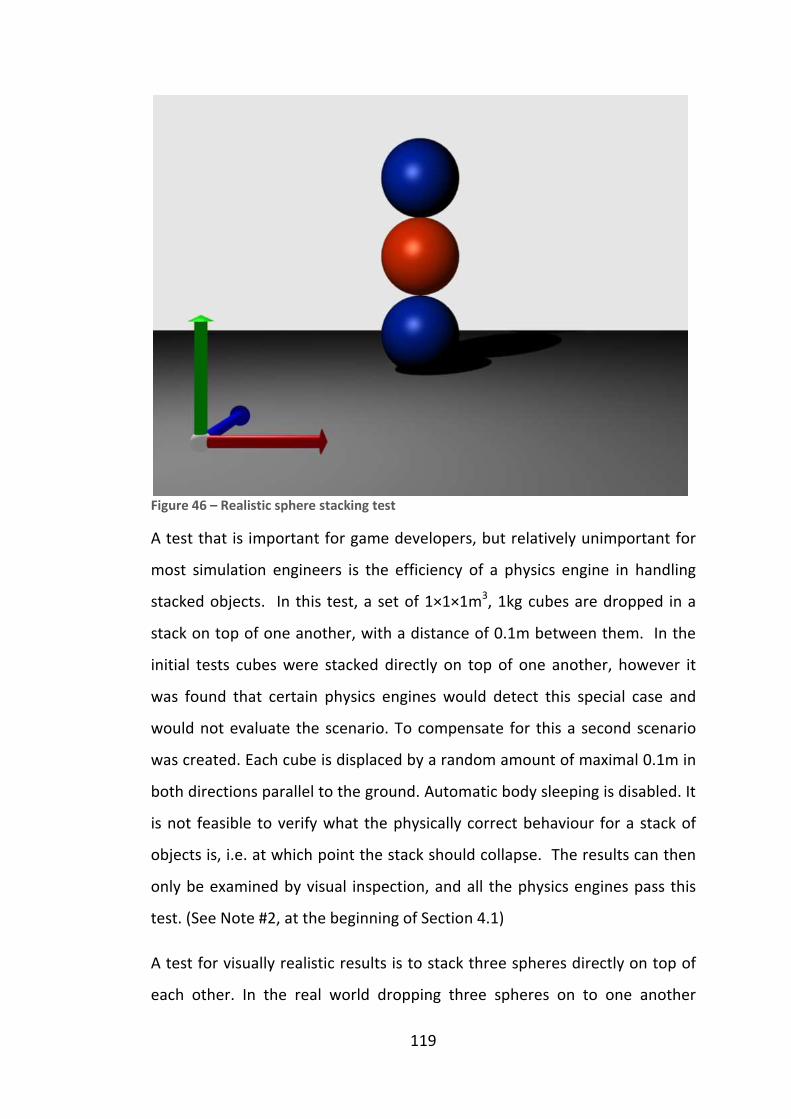
119

Figure 46 – Realistic sphere stacking test

A test that is important for game developers, but relatively unimportant for

most simulation engineers is the efficiency of a physics engine in handling

stacked objects. In this test, a set of 1×1×1m3, 1kg cubes are dropped in a

stack on top of one another, with a distance of 0.1m between them. In the

initial tests cubes were stacked directly on top of one another, however it

was found that certain physics engines would detect this special case and

would not evaluate the scenario. To compensate for this a second scenario

was created. Each cube is displaced by a random amount of maximal 0.1m in

both directions parallel to the ground. Automatic body sleeping is disabled. It

is not feasible to verify what the physically correct behaviour for a stack of

objects is, i.e. at which point the stack should collapse. The results can then

only be examined by visual inspection, and all the physics engines pass this

test. (See Note #2, at the beginning of Section 4.1)

A test for visually realistic results is to stack three spheres directly on top of

each other. In the real world dropping three spheres on to one another

120

should not result in a stack. However, every physics engine that was tested

stacked the three spheres, providing visually unrealistic results. Although the

results produced by the engines are a mathematically correct

implementation of the physics models, failure to add noise to the simulation

results in unrealistic outcomes. Since no physics engine supports any noise

models every engine fails this test.

One metric that is possible to measure is the time taken to update the

physics engine. The computation time required to update the physics engine

for the corresponding number of stack objects is illustrated in Figure 47.

Figure 47 - Computational effort of stacked objects

To give an indication of the penetration allowed by the collision system when

solving object stacks the inter penetration of one box to the box below it is

graphed in Figure 48.

0

0.2

0.4

0.6

0.8

1

1.2

1 2 3 4 5 6 7 8 9 10 11 12 13 14 15 16 17 18

Co

mp

uta

tio

n T

ime

Number of stacked objects

Computational Effort of Stacking

Bullet

Jiggle

Newton

Novodex

Tokamak

TrueAxis

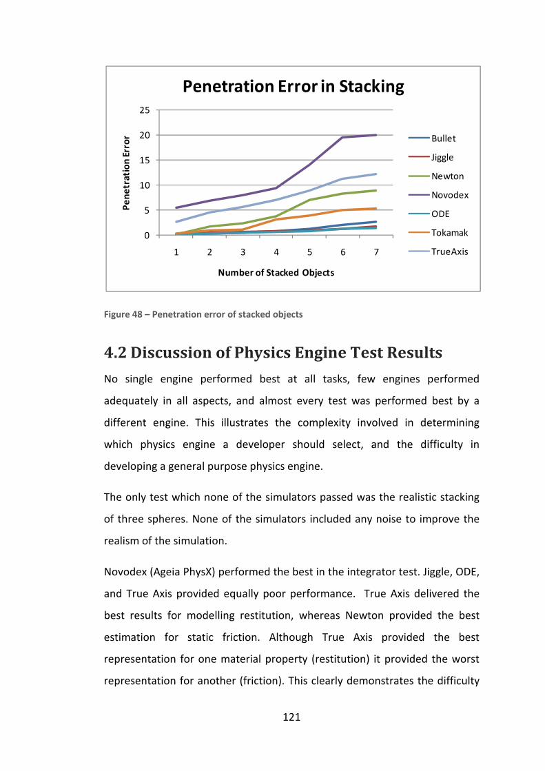
121

Figure 48 – Penetration error of stacked objects

4.2 Discussion of Physics Engine Test Results

No single engine performed best at all tasks, few engines performed

adequately in all aspects, and almost every test was performed best by a

different engine. This illustrates the complexity involved in determining

which physics engine a developer should select, and the difficulty in

developing a general purpose physics engine.

The only test which none of the simulators passed was the realistic stacking

of three spheres. None of the simulators included any noise to improve the

realism of the simulation.

Novodex (Ageia PhysX) performed the best in the integrator test. Jiggle, ODE,

and True Axis provided equally poor performance. True Axis delivered the

best results for modelling restitution, whereas Newton provided the best

estimation for static friction. Although True Axis provided the best

representation for one material property (restitution) it provided the worst

representation for another (friction). This clearly demonstrates the difficulty

0

5

10

15

20

25

1 2 3 4 5 6 7

Pe

ne

tra

tio

n E

rro

r

Number of Stacked Objects

Penetration Error in Stacking

Bullet

Jiggle

Newton

Novodex

ODE

Tokamak

TrueAxis

122

of selecting one physics engine for a particular simulated task. Even if a

simulation engineer knows that material properties will play a significant role

for their application, they must still decide on the importance of the exact

material responses to select the appropriate simulation technology.

Tokamak provided excellent results for solving large chain constraints, in

terms of computational efficiency and minimal error. It also was the most

efficient for computing stacked objects. ODE provided the best results for

constraint accuracy when configured to use a slower but accurate solver.

Newton proved to have very poor constraint solvers for this test

configuration. Generally, these tests demonstrated that accurate solutions to

the multibody constraint problem can be found, in exchange for extra

computational overhead. This is a result predicted in Chapter 2.

In the collision penetration test Jiggle and Bullet performed very well, and

TrueAxis performed very well for large integrator step sizes. Novodex,

Tokamak and ODE failed this test, allowing spheres to pass through the walls

of the pyramid. Again, this demonstrates the difficulty of adequately solving

the collision detection and response problem.

Of the open source engines the Bullet engine provided the best results

overall, outperforming even some of the commercial engines. Tokamak was

the most computationally efficient, however TrueAxis and Newton also

performed well at low update rates. Novodex is the most feature complete

system providing multiple constraint formulations, geometric

representations, rigid body, soft body and fluid simulation options.

This evaluation demonstrates the complexity involved in correctly simulating

the motion of the system. Whilst this evaluation does provide an indication

as to which physics engines would be most appropriate to a problem, it also

indicates that no physics engine provides the best choice overall. For

123

example, when evaluating which engine to use for a walking robot, it would

be difficult to argue whether the frictional effects between the ground and

the foot will hold a larger influence on the overall simulation, or the timing of

the foot-ground contacts, or the effects of an inaccurate solution to the

multibody constraints that represent the multiple linkages in the robot’s leg.

Ideally, the dynamic simulation system should provide accurate results for all

areas that are important for the simulated system. Unfortunately, such a

system does not exist. It is likely that choosing a physics engine based on one

aspect over the other will lead to unrealistic results, since no physics engine

provided accurate results across all the areas examined.

If a control system is designed purely within the context of one simulation

system, it is likely that the automated design process will create controllers

which depend on the incorrect behaviour of the underlying simulator.

Conversely, if the control system is designed within the context of multiple

simulation systems, then a successful controller will have to be designed in

such a way that it operates correctly for both the most accurate

representation of the physical reality, as well as simplified representations.

This should result in robust control systems that will operate in the most

accurate representation of the physical world.

124

5 Evolutionary Control Algorithms

Control engineering applies control theory to design systems that achieve a

desired behaviour from a dynamical system. Control problems often include

a large number of decision variables that are difficult to optimize using

traditional approaches (96). Evolutionary algorithms are robust, directed

search and optimization techniques that potentially provide superior

performance and design flexibility for optimizing control problems (96). This

chapter provides an overview of using evolutionary algorithms to optimize

control system parameters.

5.1 Control System Design

The aim of a control system is to produce a desired set of outputs affecting

the behaviour of a system from a given set of inputs and the system’s current

state. There are a number of different control algorithms, each has their

advantages and disadvantages.

5.1.1 PID Control System

A proportional-integral-derivative controller (PID controller) is a control loop

feedback mechanism (97) that attempts to correct the error between a

measured process variable and a desired set point by calculating and then

outputting a corrective action that can adjust the process accordingly. The

PID controller is based upon three parameters. A proportional term, that

determines the response to the current error, an integral term, that

determines the response to previous errors, and a derivative term, that

responds to the rate of change in the error value. These three separate terms

can be combined in any manner to produce a variant of the PID controller.

A proportional controller provides a linear response to an error by

multiplying it by the term .

125

[( = (

Where [( is the controller output ,

and ( is the error value given from the difference between the desired

set point and the current value. Equation 75 – Proportional controller

An integral controller provides a response to the error history through an

integral term T. This term can reduce the steady state error of the P

controller, but may contribute to system instability due to the response to

past values (97).

[( = 1T 6 ((7 = T 6 ((

7

Equation 76 – Integral controller

Finally, the derivative term provides a faster response to a change in the

controllers input (97).

[( =

Equation 77 – Derivative controller

The complete PID controller equation is given below:

[( = ( + T 6 ((7 +

Where is the proportional term,

T is the integral term,

and is the derivative term. Equation 78 - PID controller

PID controllers are extremely popular choices for control systems due to

their simplicity and proven effectiveness (98). However, if used alone PIDs

often provide poor performance over alternative control structures.

The performance of a single PID controller can be improved by coupling it

with another control system. If a model of the controlled system is available,

126

then a PID controller can be combined with a simple feed-forward controller

to provide reasonable results. Alternatively, the PID can be coupled with a

more advanced controller, such as a Fuzzy Logic or Spline control system, or

simply placed in cascade with another PID controller.

5.1.2 Spline Control System

Splines are piecewise polynomial functions expressed by a set of control

points (99). There are many different forms of splines, each with their own

attributes. There are two desirable properties for a spline to possess.

Continuity, so that the generated control signal translates to smooth higher

order changes and locality of the control points, to reduce the influence of

alterations of one control point to the overall shape of the spline. Two of the

most commonly used splines in computer graphics (99) have also been

applied to robotic control (100). The B-spline is defined by Equation 79. The

B-spline features the two desirable properties of locality and continuity. Each

segment of the B-spline curve is dependent on only a limited number of the

neighbouring control points. Thus, a change in the position of a distant

control point will not alter the shape of the entire spline (99)(100). The

continuity of the spline is determined by the order of the polynomial

functions utilized. A B-spline of order K is also generally CK-2

continuous. A B-

spline function with four control points s0,…,s3 parameterized by t=0,…,1, is

expressed in Equation 79.

$( = 7B7( + uBu( + 9B9( + B(

Where, B7( = − (² + (s

9 − (9 + u

Bu( = (²9 − 9 + 9

B9( = − (² + (s

9 + (9 + u

B( = − (²

Equation 79 – B-spline

127

The Hermite spline is expressed by the equations given in Equation 80. Unlike

the B-spline, the curve generated from the spline passes through the control

points that define the spline. Thus, a set of predetermined points can be

smoothly interpolated by simply setting the points as the control points for

the Hermite spline. Like the B-spline, the curve generated from the Hermite

spline is dependent only on the neighbouring control points. However, the

disadvantage of the Hermite spline is that the control point tangent values

must be specified.

The function used to interpolate the control points, given starting point p1,

ending point p2, tangent values t1 and t2, and interpolation point s, is shown

below:

$( = ℎuyu + ℎ9y9 + ℎu + ℎ³9

Where ℎu = 2 − 39 + 1 ℎ9 = −2 + 39 ℎ = − 29 +

and ℎ³ = − 9 Equation 80 – Hermite spline

A spline controller provides a simple and fast method for producing control

signals mapped from the current input state. Each spline is a separate single

dimensional system providing a single output for a single input value, and

thus can be coupled to provide higher order control systems.

128

Figure 49 – Two dimensional spline controller output space

5.2 Genetic Algorithms

A common class of evolutionary algorithms is the Genetic Algorithm (GA)

(101). Similar to other evolutionary algorithms the Genetic Algorithm makes

use of principles from Darwin’s theory of natural selection, ensuring the

survival of the fittest. The genetic algorithm progresses towards a solution to

a problem in an iterative process based from a history of potential solutions

that are manipulated by a number of biologically inspired operations.

The genetic algorithm operates on a set of encoded variables representing

the parameters for the potential solution to a problem. The parameters (or

genes) are combined together to form a string of values, referred to as a

chromosome (102). Each of these possible solutions is then assigned a

fitness value according to how optimal the solution is. The better solutions

are then selected to “reproduce” with other solutions, generating a new set

of chromosomes, which have inherited features from the chromosomes they

were created from. The least fit (worst solutions) are less likely to be selected

129

for reproduction, and thus eventually are removed from the set of

chromosomes on which the algorithm operates. In this manner the GA will

search the problem set (or feasible design space) and optimize it towards

better solutions.

The basic methodology for the genetic algorithm consists of six steps:

1. Randomly initialize a population of chromosomes

2. Evaluate the fitness of each chromosome

3. If the fitness of an individual meets the required criteria, then

terminate the algorithm.

4. Remove the lower fitness individuals

5. Generate new individuals using genetic operators, determined by a

certain selection scheme.

6. Return to step two, unless the terminating criteria has been satisfied.

Each iteration of these steps creates a new population of chromosomes. The

total set of chromosomes at one iteration of the algorithm is known as a

generation. As the algorithm progresses it searches through the solution

space, refining the solutions to find one which will fulfil (or come as close as

possible to fulfilling) the desired criteria, as described by the fitness function.

The utility of genetic algorithms is their ability to be applied to problems

without a deterministic algorithmic solution. Certain satisfiability problems

in robotic control fall under this category. For example, there is no known

algorithm to deterministically develop an optimal walking gait for a particular

robot. An approach to designing a walking gait using genetic algorithms is to

evolve a set of parameters controlling a gait generator. The parameters

completely control the type of gait that is produced by the generator. We

can assume there exists a set of parameters that will produce a suitable walk

for the robot and environment – the problem is to find such a set. Although

we do not have a way to obtain these algorithmically, we can use a genetic

130

algorithm in a simulated environment to incrementally test and evolve

populations of parameters to produce a suitable gait.

5.2.1 Fitness Functions

Each problem to be solved requires a unique fitness function describing that

problem. Given a particular chromosome, a fitness function must return a

numerical value indicating the appropriateness of the solution with respect

to the overall goal (103). For some applications, such as function optimization

problems, the fitness function will simply return the value of the function

itself.

For many applications there is no straightforward performance measurement

of the goal, and thus it must be expressed as a combination of the desired

factors. For example, if a fitness function is desired to describe how a robot

should walk, it is arguable as to what properties of the robot’s movement

describe an optimal gait. In these situations, the choice of the fitness

function will greatly influence the acceptability of the resulting solution

(104).

If a fitness function can be broken into multiple desirable components which

contribute to the overall fitness of a solution, a multi-objective genetic

algorithm can be used. The desired solution can then be selected from a

range of solutions which satisfy the fitness components individually. Multi-

objective genetic algorithms are discussed in more detail later in this chapter.

An alternative to multi-objective algorithms is to explicitly weight the

contributing components of a fitness function, to create a final fitness value

representing a weighted sum of the components. In complex problems

where it is difficult to describe an optimal solution, it may be easier to define

poor solutions and apply a penalty function (102). For example, a walking

robot may be rewarded for increasing its velocity, but penalized if this is

achieved by bringing the robot into an unstable state.

131

Fitness functions cannot always directly express the system model and may

need to be approximated. An example of this would be the motion control of

an underwater robot. The real fitness function would be based on

measurements of the movement of the real underwater robot. However, it

may not be practical to evaluate the fitness function on the real robot

thousands of times. A solution to this is to approximate the underwater

movement using 3D computational fluid dynamics (CFD) simulations. These

simulations are computationally intensive, and so the fluid behaviour may be

approximated into lower order 2D approximations (105).

If the fitness evaluations are very expensive to compute, an estimate of the

fitness of a new individual can be approximated from the fitness of the

parents of the individual and the surrounding solution space.

Figure 50 – Approximate fitness function false optimum

Although approximate fitness functions may reduce the number of fitness

evaluations required, it is very likely the GA will converge to a false optimum

due to the discrepancies between the approximate fitness function and the

real fitness function (105). Therefore, approximate fitness models can only

be used in cases where the real fitness function is also available for

verification.

False Optimum

-- Approximate Fitness Function

-- Real Fitness Function

132

5.2.2 Selection Schemes

In the natural world the organisms which reproduce the most before dying

will have the greatest influence on the next generation. In order to simulate

this effect in the genetic algorithm, a selection scheme is used. The selection

scheme determines which individuals of a given population will contribute to

form the new individuals for the next generation. There are two key concerns

with selection schemes, these are the fitness bias and the genetic spread.

The fitness bias is the absolute difference between an individual's normalized

fitness and its expected probability of reproduction. The genetic spread is

the range of possible values for the number of offspring of an individual

(106). There are two common types of selection schemes, implicit fitness

selection (e.g. Tournament selection) and explicit fitness selection (e.g.

Roulette Wheel selection) (102).

Tournament selection is an implicit fitness selection scheme that operates by

selecting two chromosomes from the available pool, and comparing their

fitness values when they are evaluated against each other. The better of the

two is then permitted to reproduce. Thus, the fitness function chosen for this

scheme only needs to discriminate between the better of two entities. To

achieve good results with tournament selection over implicit fitness selection

schemes a large population size is required, which is undesirable in

optimization problems that are computationally intensive and have moving

fitness functions (107).

Truncation selection is a simple implicit fitness selection scheme. The

population is sorted according to its fitness values and a proportion of the

individuals with the highest fitness values are selected for reproduction. This

selection scheme suffers from significant genetic bias and a loss of genetic

diversity that can cause poor performance (106).

In roulette wheel selection (s

with replacement or fitness proportionate selection

chromosome to reproduce is proportional to the fitness of the entity, and so

it has no bias (106). Thus, if the fitness value returned for one chromosome is

twice as high as the fitness value for another, it is then twice as likely to

reproduce, however its reproduction is not guaranteed as in tournament

selection. To select an in

each individual occupying a space that corresponds to its fitness value (See

Figure 51). Each individual is then

offspring.

Figure 51 – Stochastic universal sampling verses Roulette wheel selection

Stochastic universal sampling

fitness is mapped according to its fitness, however only the first individual is

selected at a random position, and then all future individuals are selected

based on an equal spacing (See

and there is minimum spread

Although genetic algorithms will

chromosomes reproduce, it has been shown that by duplicating unchanged

copies of the chromosomes into future generations, there will be a significant

increase in the convergence rate towards the solution. The term eliti

refers to the percentage of chromosomes which are transferred into the next

133

In roulette wheel selection (sometimes referred to as stochastic sampling

or fitness proportionate selection (108)) the chance for a


. Thus, if the fitness value returned for one chromosome is



selection. To select an individual the total fitness is mapped onto a line with


). Each individual is then selected at a random position to produce

Stochastic universal sampling verses Roulette wheel selection

Stochastic universal sampling is similar to roulette wheel selection in that the



based on an equal spacing (See Figure 51). This ensures that there is no bias,

and there is minimum spread (102)(106).

Although genetic algorithms will converge to a solution if all of the



increase in the convergence rate towards the solution. The term eliti


stochastic sampling

) the chance for a


. Thus, if the fitness value returned for one chromosome is



dividual the total fitness is mapped onto a line with


selected at a random position to produce

Stochastic universal sampling verses Roulette wheel selection

is similar to roulette wheel selection in that the



). This ensures that there is no bias,

converge to a solution if all of the



increase in the convergence rate towards the solution. The term elitisim


134

generation unchanged. Similarly, a steady-state GA will maintain a set

population, containing the best individuals generated during the GA’s run

and replace only a subset with new individuals.

There have been extensive comparisons of selection schemes and as a

general rule there is no single best scheme, instead the best scheme depends

on the problem type and the chosen parameter set (102). However, most

results tended to indicate that stochastic universal sampling should

outperform the roulette wheel selection approach (102).

5.2.3 Genetic Operators

The operators determine the method in which one or more chromosomes

are combined to produce a new chromosome. Traditional approaches utilize

only two operators: Mutate, and Crossover (102). Crossover takes two

individuals and divides the string into two portions at a randomly selected

point inside the encoded bit string. This produces two “head” segments and

two “tail” segments. The two tail segments for the chromosomes are then

interchanged, resulting in two new chromosomes where the bit string

preceding the selected bit position belongs to one parent, and the remaining

portion belongs to the other parent.

Figure 52 – Genetic crossover operator

The mutate operator randomly selects one bit in the chromosome string, and

inverts the value of the bit. Traditionally, the crossover operator has been

viewed as the more important of the two techniques for exploring the

135

solution space, however without the mutate operator portions of the

solution space may not be searched, as the initial chromosomes may not

contain all possible bit values (102).

Figure 53 – Genetic mutate operator

There are a number of extensions to the set of operators used. The two point

crossover operates similarly to the single point crossover described

previously, except that the chromosomes are now split in two places rather

than just one (109). The mutate operator can also be enhanced to operate on

larger portions of the chromosome than just one bit, increasing the

randomness that can be added to a search in one operation. Further

extensions rely on operating on the bit string under the assumption that

portions of the bit string represent non-binary values (such as 8 bit integer

values, or 32 bit floating point values). Two operators commonly used that

rely on this interpretation of the chromosome are the Non-Binary Average,

and the Non-Binary Creep operators (109). Non-Binary Average interprets

the chromosome as a string of higher cardinality symbols and calculates the

arithmetic average of the two chromosomes to produce the new individual.

Likewise, Non-Binary Creep treats the chromosomes as strings of higher

cardinality symbols and increments or decrements the values of these strings

by a small randomly generated amount (109).

136

Figure 54 – Non-binary average operator

5.2.4 Encoding

The encoding method chosen to transform the controller parameters to a

chromosome can have a large effect on the performance of the genetic

algorithm. Compact encoding allows the genetic algorithm to perform

efficiently, as it reduces the search space for the GA (110). There are two

common encoding techniques applied to the generation of a chromosome

(103)(109). Direct encoding explicitly specifies every parameter within the

chromosome, whereas indirect encoding uses a set of rules to reconstruct

the complete parameter space. Direct encoding has the advantages that it is

a simple and powerful representation, however the resulting chromosome

can be quite large. Indirect encoding is far more compact, yet often it only

represents a highly restrictive set of the original structures.

Regardless of which encoding technique is selected, the problem variables

must be represented in a unique binary format. The encoding mechanism

depends on the nature of the problem variables. For example, the use of a

velocity based or position based control system can be selected with a

discrete encoding. However, the controller parameters are more likely to be

represented as continuous variables.

The most common solution to encoding continuous variables is to represent

them using fixed point arithmetic (111). This can be achieved by simply

scaling a continuous value within a fixed range. A continuous value that

ranges from -1.28 to 1.28 could be multiplied by 100 to result in an 8 bit

integer representation that ranges from -128 to 128. A direct binary encoding

137

is often undesirable as multiple bits must change to represent a small

increment (e.g.: changing binary 127 to 128 requires 8 bits to flip). A solution

to this is to use Gray codes, where successive values differ by only one bit

(111).

The number of bits used to represent a variable directly affects the precision

of the resulting solution and the overall size of the search space for the GA

(110). Thus a tradeoff must be made between the solutions precision and the

size of the search. One mechanism that can alleviate this tradeoff is dynamic

parameter encoding (110). This mechanism monitors convergence statistics

from the GA to adaptively modify the length of the binary encoded variables

representation. Similar to many other modifications to the traditional GA,

dynamic parameter encoding only provides performance enhancements for

some problem types (110).

5.2.5 Staged Evolution

A number of possibilities exist in enhancing the performance of a genetic

algorithm. Staged evolution is based on the concept of behavioural memory,

and increases the GAs convergence rate by introducing a staged set of

manageable challenges (112). Initially limiting the search to a subset of the

full solution space enables an approximate solution to be determined.

Incrementally increasing the complexity of the problem will increase the

solution space, providing the possibility of increased performance as further

refinements of the solution are possible. Applying this strategy to a particular

problem task, requires that the tasks is capable of being split into further

smaller sub-tasks which can be solved in order to contribute to the overall

solution.

Staged Evolution has similar effects to other approximate fitness GAs (such

as approximate Hierarchical GAs (105)) and adaptive encoding techniques

(such as dynamic parameter encoding (110)). All of these techniques attempt

138

to reduce the computational requirements of the GA either by reducing the

search space, or reducing the cost of the GA evaluations. Whilst other

techniques are relatively general to the GA problem, Staged Evolution is

highly dependent on the nature of the problem. This enables the designer to

manually control and balance the performance of the GA with the negative

aspects of imprecise and false optimums in a task-specific manner.

5.2.6 Premature Termination

Genetic algorithms may require thousands of individuals to be evaluated

before converging to a solution. If the individual is evaluated in a full physics

simulation, it can take a long time to evaluate its fitness. Ziegler and Banzhaf

(100) introduce the concept of premature termination. During the evaluation

of an individual in a physical simulation, it may be possible to determine that

the individual has made an irrevocable error, and it is unlikely to obtain a

high fitness score. These individuals can have their evaluation terminated at

the point where the error has occurred. This saves computing time as the

entire physics simulation is not carried through to the final goal.

Figure 55 – Left - An individual that does not stray from the ideal trajectory. Right – an

individual that exceeds the acceptable variance in trajectory and can be prematurely

terminated.

For example, if an object is to move from its starting position towards a goal

any individual that strays too far from the ideal trajectory can be terminated.

Due to the momentum behind the object, it is unlikely that it will be able to

return to its goal in an acceptable manner. This is illustrated in Figure 55.

Ideal Trajectory Ideal Trajectory

x

Abortion

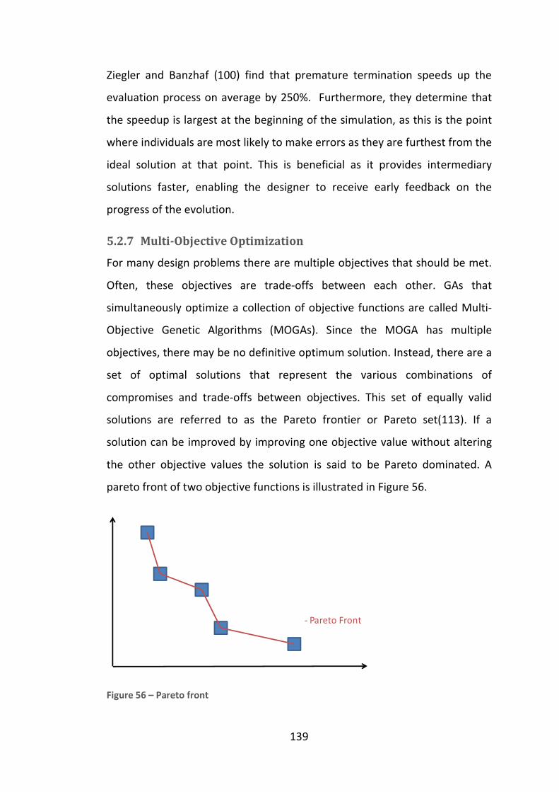
139

Ziegler and Banzhaf (100) find that premature termination speeds up the

evaluation process on average by 250%. Furthermore, they determine that

the speedup is largest at the beginning of the simulation, as this is the point

where individuals are most likely to make errors as they are furthest from the

ideal solution at that point. This is beneficial as it provides intermediary

solutions faster, enabling the designer to receive early feedback on the

progress of the evolution.

5.2.7 Multi-Objective Optimization

For many design problems there are multiple objectives that should be met.

Often, these objectives are trade-offs between each other. GAs that

simultaneously optimize a collection of objective functions are called Multi-

Objective Genetic Algorithms (MOGAs). Since the MOGA has multiple

objectives, there may be no definitive optimum solution. Instead, there are a

set of optimal solutions that represent the various combinations of

compromises and trade-offs between objectives. This set of equally valid

solutions are referred to as the Pareto frontier or Pareto set(113). If a

solution can be improved by improving one objective value without altering

the other objective values the solution is said to be Pareto dominated. A

pareto front of two objective functions is illustrated in Figure 56.

Figure 56 – Pareto front

- Pareto Front

140

Since the overall goal in a multi-objective problem is a balance of multiple

sub-objectives, the designer will often select one solution according to their

preference. The designers preferences can be defined in terms of a function

called the preference function (113).

An alternative to Pareto optimality is to define a single ideal solution point

(113). This ideal point (or utopia point) represents a solution where each sub-

objective is at its optimum. For example, if minimizing a MO problem, the

utopia point represents the point where each of the objective functions are

at their minimum.

In general, the utopian point is unattainable, however the closest possible

point to the utopian point is the best possible solution. Again, this can

involve the designers preference in defining the utopian point and the

distance measurement (e.g. Euclidean) for selecting the closest solution.

A common alternative to involving the designer in selecting preferences is to

form a global criterion (113). This is a scalar function that combines the

multiple objectives, not necessarily reflecting a designer’s preferences. The

most common approach is to use a weighted sum of the objective functions.

$ = v TT(=T´u

Where T is the scalar weighting,

and T( is the set of objective functions Equation 81 – Weighted sum

The weightings can be determined from mathematical analysis, such as the

partial weighting method, which identifies common characteristics in

objective functions and groups them to form independent weightings (113).

A simpler approach is to map the designer’s preferences to objective

weightings. This can be done via a number of techniques.

141

Ranking methods or Categorization methods(113) require the designer to

rank the importance of the objective functions and then set the weightings

with consistent increments from least to most important. Rating methods

require designers to indicate the relative importance of each objective

function. In the eigenvalue rating method (113) each unique pair of objective

functions is compared to yield a comparison matrix, and the eigenvalue of

this matrix is then used as the scaling weights.

There are three key approaches to implementing a MOGA(114). Criterion

selection approaches such as vector evaluated GA(113), where sub-

populations are evaluated one objective function at a time. Aggregation

based approaches use weighting functions to sum up the objective values

(115). Finally, Pareto based approaches such as the non-dominated sorting

GA(116) maintain the previous population and then sort the combined

population to eliminate non-dominated solutions from the next generation.

Zitler et al (114) compare a number of Multi Objective Genetic Algorithms

and find that criterion selection and aggregation approaches perform

approximately equally well, with Pareto based approaches performing best.

Marler and Arora (113) survey applied multiobjective techniques and

conclude that multiobjective approaches require significantly more

computational effort . They find that unless the nature of the problem is very

well understood, it is unlikely that the multiobjective GA will be configured in

a manner that will outperform an objective summation method or single

objective GA.

5.3 Analysis of GA performance

The conclusions found from surveys on the application of evolutionary

algorithms to engineering problems in Section 5.2 indicate that there is no

ideal algorithm configuration that will guarantee ideal performance for any

given problem. Similarly, the fields of multiobjective genetic algorithms an

approximate fitness genetic algorithms come to no conclusive finding. The

findings indicate that the performance of the GA will be task

reason the performance of a number of genetic algorithms was investigated.

The problem task was to evolve a walking gait for a simple simulated bipedal

robot.

Figure 57 – Simple Robot Model

A simple robot was modelled consisting of two regular, geometrically

identical legs, with three joints per leg. This gives a total of six degrees of

freedom. Each join has a separate cascaded controller attached, thus a total

of 6 joint controllers for eac

large feet, and lacked a complete torso. This is a highly unrealistic model of a

robot and is only used to trial and

Although multiobjective GA’s can be applied to the robot gait task, many

robotics problems, such as wall following or lane tracking are single

tasks. Marler and Arora (113)

provide benefits over single objective GAs when used with weighted sum

fitness objectives, unless they are configured for a very specific task. The

approaches developed in this thesis are intended to be general and

142

given problem. Similarly, the fields of multiobjective genetic algorithms an


findings indicate that the performance of the GA will be task-specific. For this


evolve a walking gait for a simple simulated bipedal

Simple Robot Model




of 6 joint controllers for each gait are evolved. The robot (See Figure


robot and is only used to trial and optimize the evolution process.


robotics problems, such as wall following or lane tracking are single-

(113) extensive survey find that MOGA do not




given problem. Similarly, the fields of multiobjective genetic algorithms and


specific. For this


evolve a walking gait for a simple simulated bipedal




Figure 57) had



-objective

survey find that MOGA do not




143

applicable to any robotics tasks. Therefore MOGA approaches are not

investigated.

The literature on approximate fitness functions and staged evolution imply

that there may be an advantage in these approaches in terms of reducing

computation time and improving the robustness of the evaluated controllers

(105). Premature termination should also provide a reduction in the

computation time required to evolve a controller. The influence of staged

evolution and premature termination on the fitness of the individuals

produced, and the computational speedup is investigated.

Beasley et al. (102) indicate that stochastic universal sampling should provide

benefits over roulette wheel selection and that steady state GAs and GAs

with elitism may provide benefits. Again, the performance of each GA

configuration is only found to be beneficial for certain problem tasks.

Therefore these four GA configurations are evaluated in the context of gait

controller problem. The effect of premature termination and staged

evolution on each GA is evaluated.

5.3.1 Genetic Algorithm Configurations

Four different configurations of a single objective genetic algorithm were

implemented to evolve the controller. The first was a traditional GA using

roulette wheel selection with two operators: a one-point crossover, and a

mutate operator. This configuration was used as this is a commonly

implemented version of the genetic algorithm, and hence can provide a

benchmark figure.

The second configuration employed stochastic universal sampling and

additional genetic operators. The third and fourth configurations used steady

state GA’s with low and high values of elitism respectively.

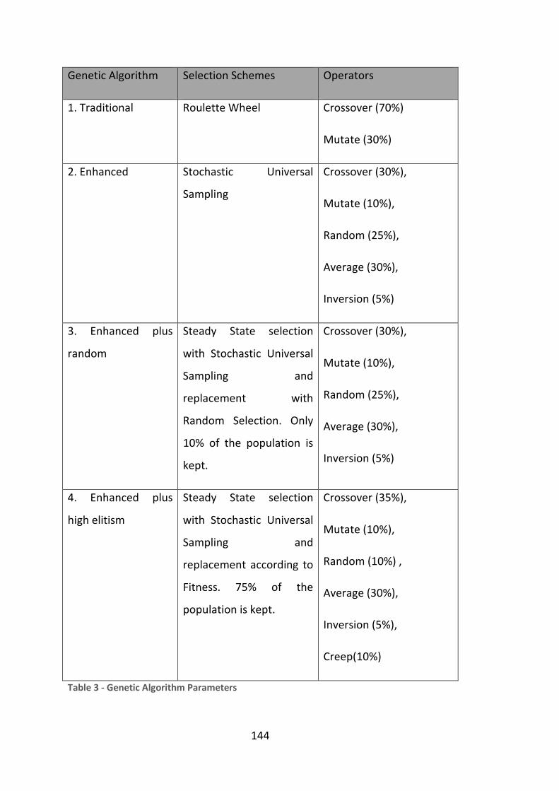
144

Genetic Algorithm Selection Schemes Operators

1. Traditional Roulette Wheel Crossover (70%)

Mutate (30%)

2. Enhanced Stochastic Universal

Sampling

Crossover (30%),

Mutate (10%),

Random (25%),

Average (30%),

Inversion (5%)

3. Enhanced plus

random

Steady State selection

with Stochastic Universal

Sampling and

replacement with

Random Selection. Only

10% of the population is

kept.

Crossover (30%),

Mutate (10%),

Random (25%),

Average (30%),

Inversion (5%)

4. Enhanced plus

high elitism

Steady State selection

with Stochastic Universal

Sampling and

replacement according to

Fitness. 75% of the

population is kept.

Crossover (35%),

Mutate (10%),

Random (10%) ,

Average (30%),

Inversion (5%),

Creep(10%)

Table 3 - Genetic Algorithm Parameters

145

To support the staged evolution, the spline controller must support a variety

of encodings. In its simplest form, each control point is at a fixed equal

distance along the spline, and only one dimension of the control point is

encoded. For the next stage of evolution the constraint of equidistant control

points along the spline is removed, and each control point is then encoded as

two values (one for each dimension – percentage walk cycle complete, and

joint input value). Finally, to enhance the smoothness of the gait, the

complete spline is encoded with two dimensional control points with tangent

information. All controller parameters are encoded in a fixed point format.

This encoding scheme allows a progressively larger chromosome to be

evolved, enabling the final gait solution to be refined until an optimal gait is

found. Encoding the control system as outlined provides compact

chromosomes, and enables the GA to perform staged evolution.

5.3.2 Genetic Algorithm Analysis

In order to determine the efficiency of each of the proposed genetic

algorithm optimizations a small test was run, in which a walking gait for the

simple robot was evolved. The gait was simulated for seven seconds, for a

maximum of thirty generations. The initial population set provided to all GA

configurations for each attempt was identical, and all tests were run on 800

MHz Pentium 3 systems running Windows NT. A number of trials were

performed for each GA, and each trial was executed ten times. All results

presented are numerical averages of all trials. The GAs were configured with

a population size of 50 individuals and used identical encoding schemes and

fitness functions.

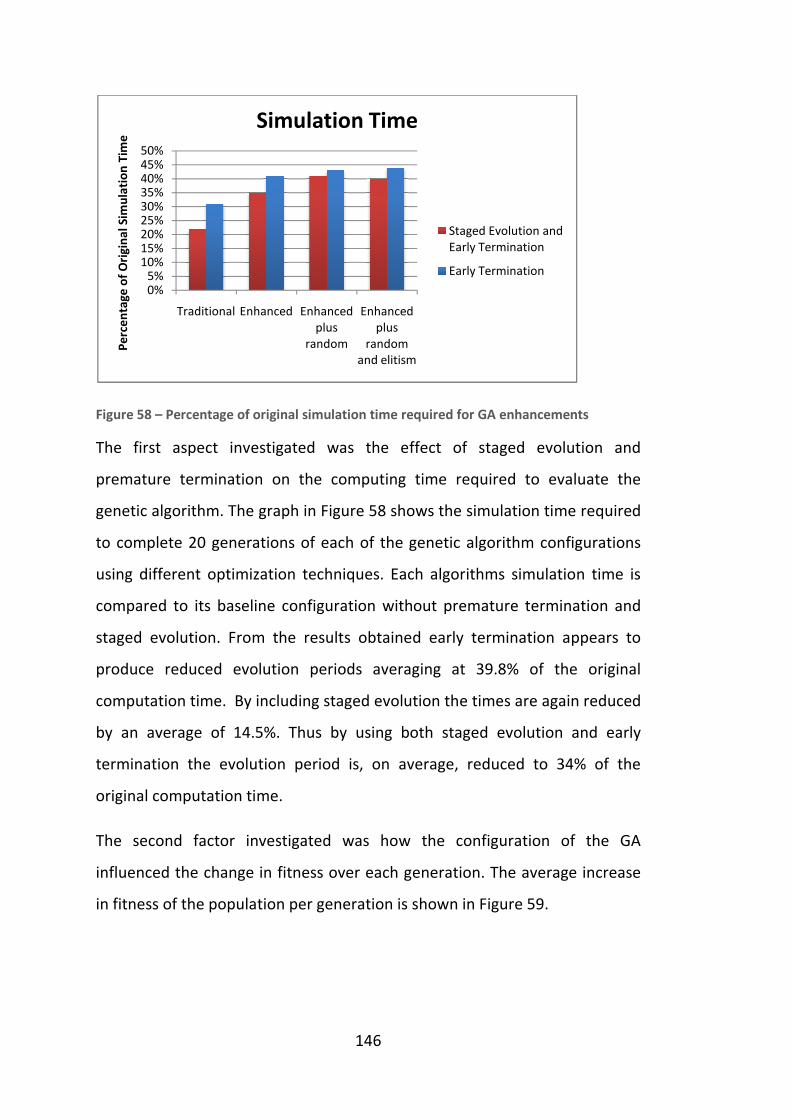
Figure 58 – Percentage of original simulation time required for GA enhancements

The first aspect investigated was the effect of staged evolution and

premature termination on the computing time required to evaluate the

genetic algorithm. The graph in

to complete 20 generations of each of the genetic algorithm configurations

using different optimization techniques. Each algorithms simulation time is

compared to its baseline configuration without premature

staged evolution. From the results obtained early termination appears to

produce reduced evolution periods averaging at 39.8% of the original

computation time. By including staged evolution the times are again reduced

by an average of 14.5%. Thus by using both staged evolution and early

termination the evolution period is, on average, reduced to 34% of the

original computation time.

The second factor investigated was how the configuration of the GA

influenced the change in fitness over each

in fitness of the population per generation is shown in

0%5%

10%15%20%25%30%35%40%45%50%

Traditional Enhanced

Pe

rce

nta

ge

of

Ori

gin

al

Sim

ula

tio

n T

ime

Simulation Time

146

Percentage of original simulation time required for GA enhancements



genetic algorithm. The graph in Figure 58 shows the simulation time required



compared to its baseline configuration without premature termination and




%. Thus by using both staged evolution and early



influenced the change in fitness over each generation. The average increase

in fitness of the population per generation is shown in Figure 59.

Enhanced Enhanced

plus

random

Enhanced

plus

random

and elitism

Simulation Time

Staged Evolution and

Early Termination

Early Termination

Percentage of original simulation time required for GA enhancements



shows the simulation time required



termination and




%. Thus by using both staged evolution and early



generation. The average increase

147

Figure 59 – Average Fitness Increase per Generation

The early termination causes the conventional genetic algorithm to decrease

its average increase in fitness, whilst the other forms of genetic algorithms

appear to gain in fitness. A possible explanation for the abnormal result from

the conventional algorithm is that it relies on the randomness of other

chromosomes in order to be able to generate new chromosomes with

increased fitness. Each of the other genetic algorithms contain either an

operator which can introduce randomness (random replacement), or a

selection scheme which increases randomness (random selection).

For staged evolution with early termination the fitness per generation greatly

increases for the first two forms of the genetic algorithm (conventional &

enhanced), but the steady state forms do not benefit. The GA configurations

using random selection take longer to converge towards a solution, thus,

when the staged evolution takes place in generation 10, the population is not

close enough to a solution to be able to benefit from moving to the next

stage. The other two forms of GA have somewhat converged by this time,

and thus they can take advantage from the next stage.

From the results obtained it would indicate that early simulation termination

can provide significant reductions in evolution times, and genetic algorithms

0

0.05

0.1

0.15

0.2

0.25

Traditional Enhanced Enhanced

plus

random

Enhanced

plus

random and

elitism

Average Fitness Increase per

Generation

Full Simulation

Early Termination

Staged Evolution and

Early Termination

148

which produce enough randomness will not be adversely affected by having

the worse chromosomes terminated. The ability to take advantage of the

staged evolution process appears to depend on the current status of the

population of the GA. If the population has begun to converge, then the

staged evolution opens up a new prospect for higher rating fitness

chromosomes.

For all cases the increase in fitness was highest for the enhanced genetic

algorithm, whereas the performance gain over the traditional approach for

the other configurations varied. Since staged evolution combined with

premature termination provided equal or superior fitness performance to

the full simulation in all cases, yet dramatically reduced computation time,

(117) this form of GA will be employed for all experiments.

149

6 Bipedal Robot Control Experiments

Legged robots exhibit a number of advantages for locomotion (118). The

mobility offered by legged vehicles is far greater than that of wheeled or

tracked vehicles, as they are not limited to paved terrain. The increased

mobility offered allows for a far larger range of applications to legged

vehicles. Another incentive for exploring the use of legs for locomotion is

that it provides an insight to the systems responsible for human and animal

locomotion. Humans are capable of complex movements, whilst maintaining

orientation, balance and speed. Robots that could mimic human movements

could seamlessly integrate with the human world, enlarging the number of

possible applications for legged vehicles. This makes the study of bipedal

locomotion particularly attractive.

Although there are a multitude of existing locomotion control techniques and

well described design processes, the automated generation of these

controllers for robots provides significant advantages. Often, the design

process is quite complex, time consuming to perform, and requires the

control system to be completely redesigned for small alterations to the robot

(23).

By evolving the locomotion controller the robot designer is alleviated from

the controller design process. The control system becomes more flexible, as

the robot can improve its controller to cope with environmental or structural

changes. The resulting controllers are more adaptive to the robot’s

environment, more robust, more flexible, and can provide superior

performance to human designed controllers (23).

150

6.1 Physics Simulation Problems for Legged

Robots

Using a simulator to accurately model a legged robot may create a number of

difficulties. Bipedal locomotion is arguably the most complex legged

locomotion to control and simulate. The balance and control of a bipedal

robot is highly dependent on the ground reaction forces exerted under the

feet. The two main problem areas are:

• Accurately calculating the solution to the link constraints that

represent the dynamics of each degree of freedom in the robot

• Accurately calculating the interaction between the robot’s foot and

the ground.

Whilst both of these topics were discussed in general in the Dynamic

Simulation section of this thesis there are some more specific issues relating

to modelling a legged robot. Solving the robot’s link constraints accurately is

a well studied problem and an accurate solution can be achieved through the

use of a high order integrator with a reduced coordinate constraint solver

(Such as Featherstone’s articulated body algorithm (58)). However,

accurately calculating the correct response to the foot-ground interaction is

very difficult. In order to have accurate collision detection, a continuous

collision detection system is desirable. However, employing higher order

integrators can prove difficult with a continuous collision approach, due to

the complexities involved in a correct implementation (31). As a result, there

is often a trade-off between the collision detection system and the accuracy

for solving the constraints.

Assuming that a physics simulator is capable of determining the exact

geometric colliding areas, calculating the correct response to the collision is

problematic. Constraint based methods will typically formulate a linear

complimentary problem (LCP) to calculate the contact forces that comply

with the entire robot’s linkage

constraint based methods is still an open problem, often requiring an

increasing set of active contacts. When considering friction, the convexity of

the LCP disappears and a correct solution cannot be guarante

must be represented with a

undesirable effects. As the set of active contacts employed by the physics

engine increases, the likelihood of an unstable solution also in

If two objects penetrate, then the physics simulator must correct the position

of the object, usually by applying an impulse.

has penetrated the ground plane. The simplest approach to solving the

penetration condition is simply to apply a linear projection to generate the

direction of the impulse

resolution to the collision. A more physically realistic solution is to apply a

non-linear response that contains an angular impulse

Figure 60 – Possible collision responses. From left to right: p

non-linear projection and a physically accurate result.

Applying a non-linear response can create some additional problems, such as

missing situations where new contact points should be generated, or altering

the penetration depth of the other contact points on the body. Both of these

situations are illustrated in

has penetrated the ground

typical contact resolution algorithm will select the contact point with the

greatest penetration depth and resolve that point. This process can then be

151


with the entire robot’s linkage structure. Efficient contact determination for



the LCP disappears and a correct solution cannot be guarante

must be represented with a polyhedral approximation creating further


engine increases, the likelihood of an unstable solution also in


of the object, usually by applying an impulse. Figure 60 illustrates a box tha



direction of the impulse (119). This results in a physically unrealistic

lution to the collision. A more physically realistic solution is to apply a

linear response that contains an angular impulse (119).

Possible collision responses. From left to right: penetration, linear projection,

linear projection and a physically accurate result.

linear response can create some additional problems, such as


depth of the other contact points on the body. Both of these

situations are illustrated in Figure 61. The left situation depicts a body that

has penetrated the ground plane and has generated two contact points. A




structure. Efficient contact determination for



the LCP disappears and a correct solution cannot be guaranteed (37). Friction

approximation creating further


engine increases, the likelihood of an unstable solution also increases.


illustrates a box that



. This results in a physically unrealistic

lution to the collision. A more physically realistic solution is to apply a

.

enetration, linear projection,

linear response can create some additional problems, such as


depth of the other contact points on the body. Both of these

. The left situation depicts a body that

plane and has generated two contact points. A



repeated and eventually the body will come to rest on the

the complexity of maintaining other constraints and an acceptable

computation time, the number of iterations in this stage is typically limited,

and thus it is unlikely a completely satisfied condition will be met by the end

of a timestep.

This iteration process is further complicated by the possibility of introducing

new contact points. Since collision detection and contact generation is a

computationally expensive task, it is not practical to repeat it during each

step in the constraint resolution process. There are a number of contact

resolution and update algorithms available that try to minimize the

influences of these problems, however none can completely solve the

contact penetration problem.

Figure 61 – Contact resolution. Left: repeating resolutions. Right: Missed contact.

6.1.1 Multiple Simulators

Since the interpenetration problem cannot be accurately solved, an

approximate solution is always provided by the physics simulator. Often this

results in new, or unresolved penetrating contacts at the end of a time step.

152

repeated and eventually the body will come to rest on the surface. Due to







esolution process. There are a number of contact



contact penetration problem.

tact resolution. Left: repeating resolutions. Right: Missed contact.

Multiple Simulators



solved penetrating contacts at the end of a time step.

surface. Due to







esolution process. There are a number of contact



tact resolution. Left: repeating resolutions. Right: Missed contact.



solved penetrating contacts at the end of a time step.

153

A physics engine may over-compensate for this situation in the next time

step by applying a large impulse to the body.

This causes two problems for evolving a simulated robot controller. First, the

physically unrealistic behaviour of the simulator may result in an evolved gait

that is not able to transfer to reality. A common example of this in an evolved

bipeds behaviour is a where a foot interpenetrates to great depth, causing

the physics engine to provide a large impulse to correct the interpenetration.

In turn, this causes the robot to gain an unrealistic amount of forwards or

upwards momentum.

Second, an evolutionary algorithm is extremely good at identifying and

exploiting any niche advantages available in the evolutionary problem.

Typically, this will result in the EA locating a solution involving the robot’s

foot penetrating the terrain, consequently generating a large forwards

impulse. This can generate a fitness value far greater than those available to

solutions that do not profit from large interpenetrations. As a result, the EA

will often optimize the controller to cause large interpenetrations and come

to rely on a set of physically unrealistic solutions

Using multiple simulation systems ensures that this particular aspect of the

physics based simulation is unlikely to occur. Each physical simulator employs

different algorithms for solving the contact penetration problem, so it is very

unlikely that a single solution will benefit from a deep penetration impulse

across all simulators.

6.2 Evolving Control Architectures for Bipedal

Locomotion

There are a number of control systems that are applicable to the objective of

robot locomotion. Possible control systems range from simple oscillators

154

(120) to simple assembly programs (121) to neural networks (23). The

simplest oscillators consist of a set of sinusoidal function generators whose

outputs are combined to generate the control signal for an actuator. These

systems can represent a range of outputs by altering the phase and

amplitude of the sinusoids (120). However, these systems are generally

incapable of expressing the complexity required for sustained locomotion

(122). Thus, more complicated forms of control are desirable.

A common technique for maintaining bipedal stability is the use of the Zero

tipping Moment Point (ZMP) constraint. The ZMP is the point on the ground

where the sum of all the moments of the active forces is equal to zero (See

Figure 63). If the ZMP is within the support polygon formed by the feet, then

the robot will be stable. If the ZMP leaves that region the robot will begin to

fall. Using this constraint with the combination of pressure sensors has been

the key to the walking control of robots such as Honda’s ASIMO (123). The

disadvantage of this technique is that the ZMP constraint is too tight,

resulting in limited gaits, and it will only apply to legged characters and

cannot be applied to general morphologies (e.g. snakes).

Figure 62 – Bipedal robot control algorithms Figure 63 – ZMP

Biped Control

Algorithms

Pattern BasedAlgorithmic

Oscillators

Neural Networks

Splines

State Machines

ZMP

Genetic Program

n

COM

Inertial force

Floor reaction

mg

-ma

155

Another common technique for locomotion control is the use of state

machines (124). This control strategy has been successfully demonstrated for

a large range of morphologies and applications (124)(125). Yin et al. (124)

presented a state machine based approach for the control of virtual bipedal

characters. The disadvantage to the state based approach is that an

appropriate number of states must be constructed for differing gaits and

morphologies. Yin et al. inserted extra “dummy” states to the control system

to enable the transition between different gaits for the same morphology.

This approach would not scale to a general morphological configuration.

Neural networks have demonstrated stable control for a variety of

morphological configurations of both robots and virtual characters

(23)(104)(126). Typically, neural control of legged characters mimics the

central pattern generator seen in real animals. The automatic generation and

optimization of locomotion gaits has been demonstrated for a variety of

configurations (23)(104). This makes neural networks an attractive choice for

controlling generic robot configurations.

Genetic algorithms were applied to the evolution of neural controllers for

robot locomotion by numerous researchers (120)(125)(127). Lewis et al.

(125) successfully generated locomotion patterns for a hexapod robot using a

simple traditional genetic algorithm with one point crossover and mutate.

Isjpreet (127) evolved a controller for a simulated salamander using an

enhanced genetic algorithm. The large number of experiments in this area

clearly indicates that genetic algorithms are capable of evolving neural

controls that can describe legged robot locomotion.

The genetic programming approach has been shown to successfully generate

locomotion patterns for various control strategies. Banzhaf et al. (121)

demonstrated the pure genetic programming approach to develop assembly

programs for robot control. The system was then expanded to control a

156

hexapod robot (100) using a B-Spline based approach. This demonstrated

that both the genetic programming approach and the genetic algorithm

approach are capable of evolving adequate control systems for legged

locomotion (127).

Parker et al. (128) explored the use of cyclic genetic algorithms for

locomotion control of a small hexapod robot. Their system demonstrated

that the cyclic nature needed to generate the oscillatory motions necessary

for legged robot locomotion could be abstracted from the control system and

transferred and encoded into the genetic algorithms chromosomes.

Since the overall goal for the system is to develop control architectures for a

varied number of systems it is desirable to have separable controllers, whose

complexity can be increased incrementally. This allows for more efficient

evolution. It is also desirable to have a simple control structure that can be

easily interpreted by a human for debugging, analysis and validation

purposes.

Each of the outlined control strategies has its advantages and disadvantages.

Simple oscillators are not capable of expressing the range of motions

required by most applications, and common algorithmic approaches are tied

to the morphological or gait structure. Neural networks provide flexible

control, but are difficult to manipulate manually. A spline based control

system provides a greater range of motions than simple oscillators, whilst

also providing a control structure that is separable, human understandable,

and can have its complexity incrementally increased. Previous approaches

have demonstrated the automated generation of spline-based gait control

systems for simulated and real robots (100) (129). Hence a spline controller

was selected for the biped control task.

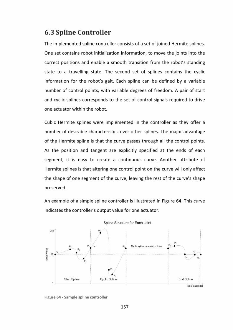
157

6.3 Spline Controller

The implemented spline controller consists of a set of joined Hermite splines.

One set contains robot initialization information, to move the joints into the

correct positions and enable a smooth transition from the robot’s standing

state to a travelling state. The second set of splines contains the cyclic

information for the robot’s gait. Each spline can be defined by a variable

number of control points, with variable degrees of freedom. A pair of start

and cyclic splines corresponds to the set of control signals required to drive

one actuator within the robot.

Cubic Hermite splines were implemented in the controller as they offer a

number of desirable characteristics over other splines. The major advantage

of the Hermite spline is that the curve passes through all the control points.

As the position and tangent are explicitly specified at the ends of each

segment, it is easy to create a continuous curve. Another attribute of

Hermite splines is that altering one control point on the curve will only affect

the shape of one segment of the curve, leaving the rest of the curve’s shape

preserved.

An example of a simple spline controller is illustrated in Figure 64. This curve

indicates the controller’s output value for one actuator.

Figure 64 - Sample spline controller

158

In order to evolve the spline controller with a genetic algorithm, the

controller’s parameters need to be encoded into chromosome

representations. To enable support for staged evolution, the controller needs

to be specifically designed, such that the evolution can proceed in this

manner. The encoded spline controller treated each control point value as a

8 bit fixed point number. In the initial phase of evolution, the control point

locations within the walking cycle time were equally distributed. This

provided each control point with only one degree of freedom and reduced

the available solution space, but also significantly reduced the complexity of

the chromosome required to describe the controller. In the following stage of

evolution, the equally distributed time constraint was dropped, providing the

control points with an additional dimension of freedom. Finally the tangent

values for the control points in the spline were added to the chromosome,

allowing final refinement of the solution. The output of the spline controller

is coupled to a PID controller. If the spline control system is directly

connected to the joint angles, then over time, the accumulated errors from

the open loop control cause the gait to deviate from the desired gait. This is

illustrated in Figure 65, where a simple simulated robot’s torso is slowly

dropping towards the ground.

Figure 65 – Walking gait with open loop control

6.3.1 Sensory Feedback

Without any feedback the control system for the robot can not react to any

changes in the environment. Feedback can be used to improve the stability

of the robot’s gait and correct any deviations from the desired path.

159

Figure 66 – Walking gait with closed loop control

In order to incorporate sensor feedback information into the spline

controller, another dimension must be added to the controller. The extended

control points specify their locations within both the gaits cycle time, and the

feedback value. This results in a set of control surfaces for each actuator. The

number of control points required for the simple spline controller is given by:

#(4 + a

Where , a is the number of actuators

i is the number of control points in the initialization spline

c is the number of control points in the cyclic spline Equation 82 – Simple spline controller complexity

Extending the controller to include feedback in this form significantly

increases the number of control points required as indicated below.

#(4 + a$

Where f is the number of control points used to sample the feedback Equation 83 – Extended spline controller complexity

The actuator evaluates the desired output value from the enhanced

controller as a function of both the cycle time and the input reading from the

sensor.

Chapter 3 presented a wide range of sensors that can provide a variety of

feedback signals ranging from angular velocity to distance readings. In adding

a sensor to a robot the most appropriate sensor type and the best position

for the sensor must be determined.

After some initial experimentation, the most appropriate sensory feedback

was found to be the torsos inclination towards the ground plane. This can be

160

measured with an inclinometer attached to the torso of the robot. Thus, the

resultant controller was expressed in terms of the percentage cycle time, the

torsos inclination angle, and the output control signal.

6.4 Gait Controller Evolved in a High Fidelity

Simulator

To ascertain the issues related to the modelling, simulation, and evolution of

a bipedal robot control system an initial test was performed using a robotics

specific simulator. A motor model for the robot was constructed, and a

number of aspects of the evolutionary process were investigated.

6.4.1 Target Hardware

The target hardware for the controller is a small humanoid robot called

Andy(97) (see Figure 67). Cost and weight were important design

considerations in Andy’s development. As a result Andy stands approximately

350mm tall, and weighs around 1400g. Andy has 10 degrees of freedom in

his legs, and each joint is powered by Hi-Tec 945 MG servos (130). The Hi-Tec

servo specifications are listed in Table 4. Links are made from 3mm thick

aluminium flat plate and are used to connect the plastic shafts of the servos

directly to the next link. These connections result in a substantial amount of

inherent flexibility.

161

Figure 67 – Andy Robot

Andy can be equipped with a number of sensors, including a color camera,

PSDs, inclinometers, gyroscopes and pressure sensors. The pressure sensors

are permanently mounted on Andy’s feet, which are constructed from three

metal “toes”. Each toe has two strain gauges that are used to produce a

voltage in proportion to the applied force.




Deadband Width 4 µsec

Operating Speed 0.16 sec / 60° No load

Operating Angle 45° / 400 µsec Table 4 – HiTec servo specifications

The biped’s processing requirements are provided by an EyeBot MK3

controller, an inexpensive but powerful platform(97). The controller is based

EyeBot controller

Side hip joints

Bend hip joints

Bend ankle joints

Side ankle joints

90°- twisted Aluminum link

Aluminium link

Metal strip toes

Knee joints

162

on a 25 MHz 32 bit Motorola 68332 chip, has a LCD display, four buttons,

parallel and serial ports, as well as 8 digital inputs and outputs and 8

additional analog inputs.

6.4.2 Simulation Model

The robot was modelled using the Dynamechs(131) simulation package. This

simulator provides a highly accurate, high order (5th

) adaptive integration

scheme based on a reduced coordinate method. Bodies and constraints must

be specified in modified Denavit-Hartenberg coordinates. The collision

system is constrained to heightfield surfaces and employs penalty based

constraints. The package has been used in high fidelity simulations for a

number of robots, including underwater walking robots (131).

A schematic of the robot’s legs are illustrated in Figure 68. The robot model

required by Dynamechs was constructed using the RobotBuilder(132)

package. For each link, the simulator requires information including its type,

relative position and orientation, mass, centre of mass, and inertia matrix.

Bodies are not modelled separately to the links.

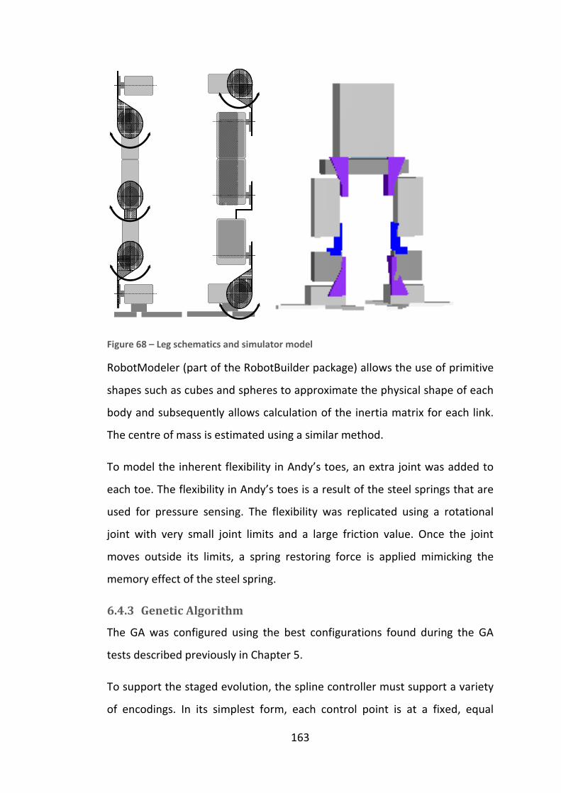
163

Figure 68 – Leg schematics and simulator model

RobotModeler (part of the RobotBuilder package) allows the use of primitive

shapes such as cubes and spheres to approximate the physical shape of each

body and subsequently allows calculation of the inertia matrix for each link.

The centre of mass is estimated using a similar method.

To model the inherent flexibility in Andy’s toes, an extra joint was added to

each toe. The flexibility in Andy’s toes is a result of the steel springs that are

used for pressure sensing. The flexibility was replicated using a rotational

joint with very small joint limits and a large friction value. Once the joint

moves outside its limits, a spring restoring force is applied mimicking the

memory effect of the steel spring.

6.4.3 Genetic Algorithm

The GA was configured using the best configurations found during the GA

tests described previously in Chapter 5.

To support the staged evolution, the spline controller must support a variety

of encodings. In its simplest form, each control point is at a fixed, equal

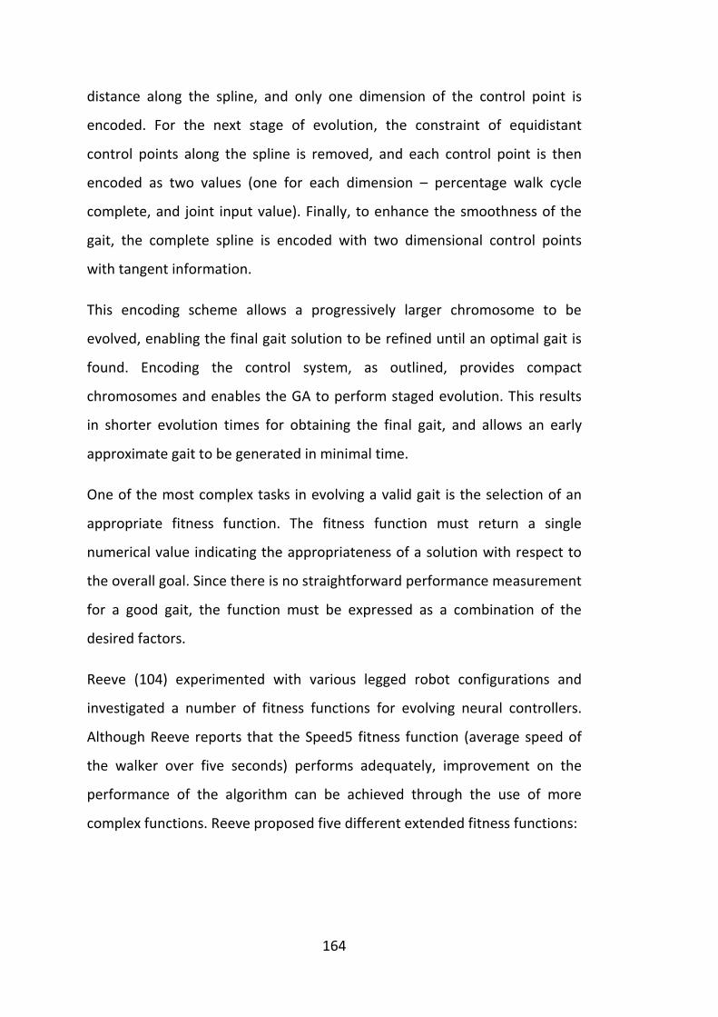
164

distance along the spline, and only one dimension of the control point is

encoded. For the next stage of evolution, the constraint of equidistant

control points along the spline is removed, and each control point is then

encoded as two values (one for each dimension – percentage walk cycle

complete, and joint input value). Finally, to enhance the smoothness of the

gait, the complete spline is encoded with two dimensional control points

with tangent information.

This encoding scheme allows a progressively larger chromosome to be

evolved, enabling the final gait solution to be refined until an optimal gait is

found. Encoding the control system, as outlined, provides compact

chromosomes and enables the GA to perform staged evolution. This results

in shorter evolution times for obtaining the final gait, and allows an early

approximate gait to be generated in minimal time.

One of the most complex tasks in evolving a valid gait is the selection of an

appropriate fitness function. The fitness function must return a single

numerical value indicating the appropriateness of a solution with respect to

the overall goal. Since there is no straightforward performance measurement

for a good gait, the function must be expressed as a combination of the

desired factors.

Reeve (104) experimented with various legged robot configurations and

investigated a number of fitness functions for evolving neural controllers.

Although Reeve reports that the Speed5 fitness function (average speed of

the walker over five seconds) performs adequately, improvement on the

performance of the algorithm can be achieved through the use of more

complex functions. Reeve proposed five different extended fitness functions:

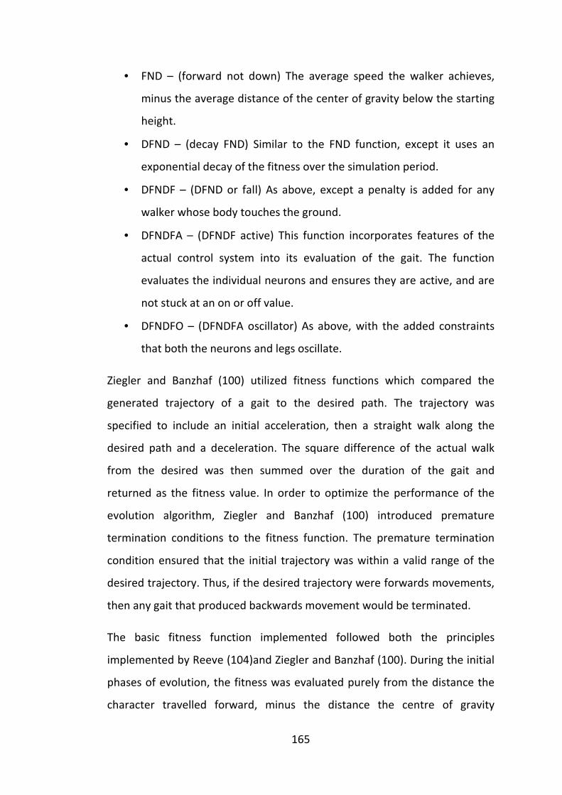
165

• FND – (forward not down) The average speed the walker achieves,

minus the average distance of the center of gravity below the starting

height.

• DFND – (decay FND) Similar to the FND function, except it uses an

exponential decay of the fitness over the simulation period.

• DFNDF – (DFND or fall) As above, except a penalty is added for any

walker whose body touches the ground.

• DFNDFA – (DFNDF active) This function incorporates features of the

actual control system into its evaluation of the gait. The function

evaluates the individual neurons and ensures they are active, and are

not stuck at an on or off value.

• DFNDFO – (DFNDFA oscillator) As above, with the added constraints

that both the neurons and legs oscillate.

Ziegler and Banzhaf (100) utilized fitness functions which compared the

generated trajectory of a gait to the desired path. The trajectory was

specified to include an initial acceleration, then a straight walk along the

desired path and a deceleration. The square difference of the actual walk

from the desired was then summed over the duration of the gait and

returned as the fitness value. In order to optimize the performance of the

evolution algorithm, Ziegler and Banzhaf (100) introduced premature

termination conditions to the fitness function. The premature termination

condition ensured that the initial trajectory was within a valid range of the

desired trajectory. Thus, if the desired trajectory were forwards movements,

then any gait that produced backwards movement would be terminated.

The basic fitness function implemented followed both the principles

implemented by Reeve (104)and Ziegler and Banzhaf (100). During the initial

phases of evolution, the fitness was evaluated purely from the distance the

character travelled forward, minus the distance the centre of gravity

166

lowered. This is a combination of aspects Reeve’s FND and Zieglers

premature termination conditions (100)(104). During later phases of

evolution, the average speed at which the robot moved and the distance the

robot wavered from the desired path were incorporated. Finally, the distance

the robot was at termination from its desired goal was taken into

consideration, to emulate the effect of Reeve’s DFND.

In order to decrease the evolution time, two terminating conditions were

added to the fitness functions. Termination would occur if the torso (main

reference point of the robot) touched the ground (i.e. the robot fell over), or

if the torso was significantly higher than its original start position (to

discourage jumping).

6.4.4 High Fidelity Simulation Gaits

Four different gaits were evolved in the high fidelity simulation. Evolving the

gaits for a high fidelity simulation is very computationally intensive. Evolving

a single gait required more than one week of computing time on a cluster of

5 AMD 2600+ PCs running Windows XP. One of these gaits is illustrated in

Figure 69 and Figure 70. They illustrate the same evolved control program

executing on the real and simulated Andy robot.

Figure 69 depicts the simulated robot movements. The robot achieves

locomotion by initially pressing downward with its left toes, causing the

robot to tilt to its right (Figure 69.2). The robot then drags its left foot along

the ground in front of it. The robot then presses downwards with its right

toes and lifts its right foot off the ground, then places it in front of it. This

cycle repeats itself to produce a slow forwards walk.

The figures show a relatively close mapping between the simulated robot

and the physical robot. This is a result one would expect from a high fidelity

simulator. One significant discrepancy between the simulated and physical

walks is illustrated in Figure 69.4 and Figure 70.4. This difference between

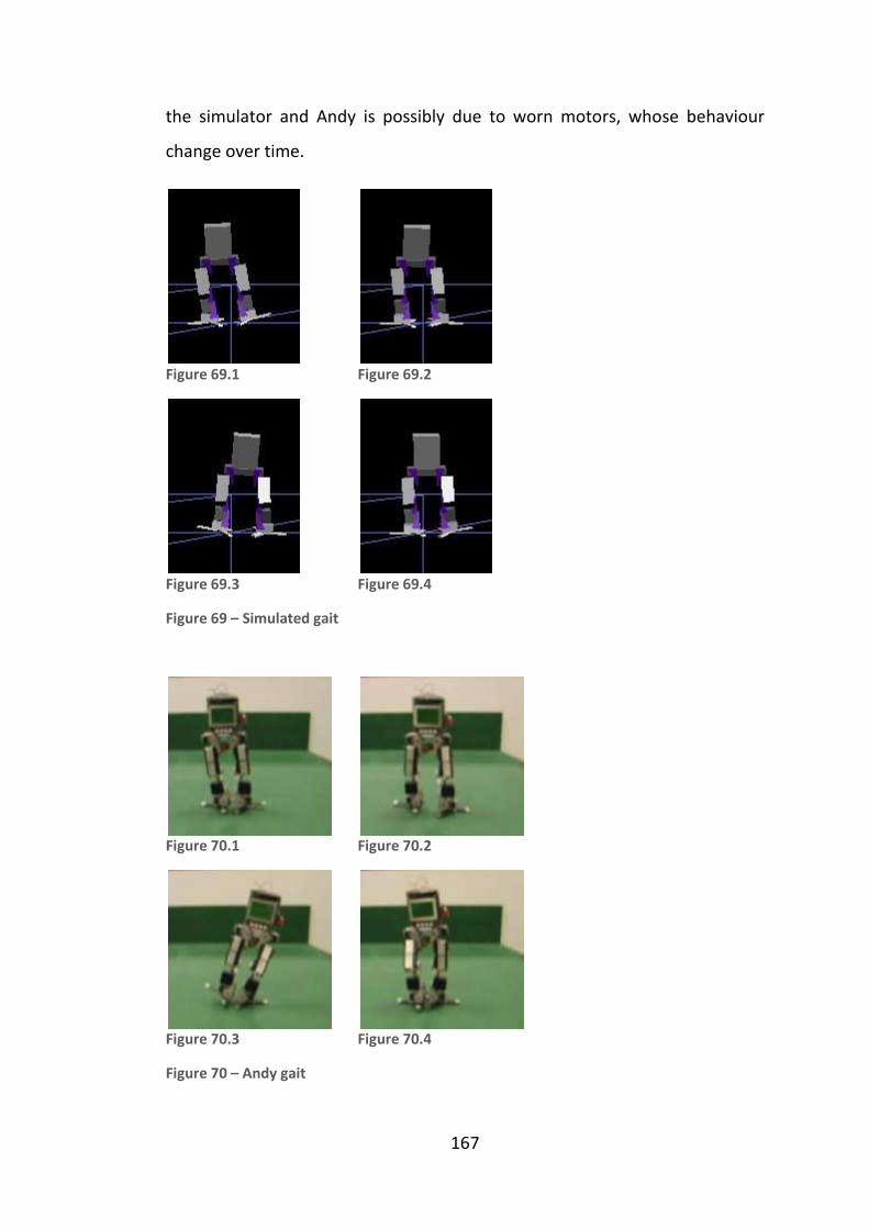
167

the simulator and Andy is possibly due to worn motors, whose behaviour

change over time.

Figure 69.1

Figure 69.2

Figure 69.3

Figure 69.4

Figure 69 – Simulated gait

Figure 70.1

Figure 70.2

Figure 70.3

Figure 70.4

Figure 70 – Andy gait

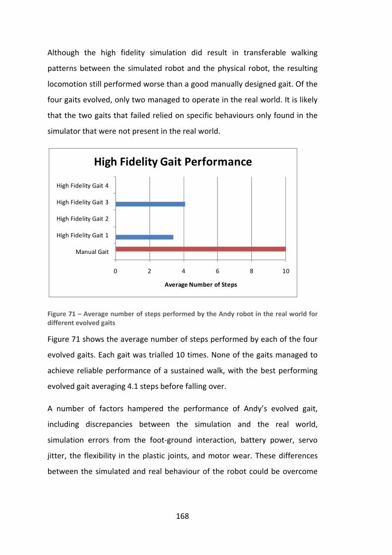
168

Although the high fidelity simulation did result in transferable walking

patterns between the simulated robot and the physical robot, the resulting

locomotion still performed worse than a good manually designed gait. Of the

four gaits evolved, only two managed to operate in the real world. It is likely

that the two gaits that failed relied on specific behaviours only found in the

simulator that were not present in the real world.

Figure 71 – Average number of steps performed by the Andy robot in the real world for

different evolved gaits

Figure 71 shows the average number of steps performed by each of the four

evolved gaits. Each gait was trialled 10 times. None of the gaits managed to

achieve reliable performance of a sustained walk, with the best performing

evolved gait averaging 4.1 steps before falling over.

A number of factors hampered the performance of Andy’s evolved gait,

including discrepancies between the simulation and the real world,

simulation errors from the foot-ground interaction, battery power, servo

jitter, the flexibility in the plastic joints, and motor wear. These differences

between the simulated and real behaviour of the robot could be overcome

0 2 4 6 8 10

Manual Gait

High Fidelity Gait 1




Average Number of Steps

High Fidelity Gait Performance

169

by employing a more robust control strategy that takes advantage of the

multiple simultaneous simulation paradigm.

6.5 Gait Controller Evolved with Multiple

Simulators

The same problem was again solved on a different robot that would enable a

more accurate comparison between a single simulator and the multiple

simulator approach.

6.5.1 Target Hardware

The target hardware for the controller is the following model to Andy, a small

humanoid robot called Andy 2(97) (see Figure 72). Again, cost and weight

were important design considerations in Andy 2’s development. Unlike the

original Andy, Andy2 is constructed with digital servos which can provide a

positional feedback reading. Therefore, the specially designed feet that

supported the pressure sensors on the original Andy, were no longer

required. Andy2 stands approximately 350mm tall and weighs around 700g.

Andy has five degrees of freedom in each leg, and each joint is powered by

AI1001 digital servos (133). The AI1001 servo specifications are listed in Table

5. Links are made from 3mm thick plastic connectors that directly link the

servo motors together. As with the original Andy, these connections result in

a substantial amount of inherent flexibility.

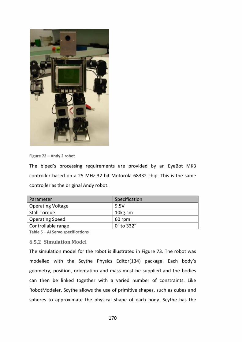
170

Figure 72 – Andy 2 robot

The biped’s processing requirements are provided by an EyeBot MK3

controller based on a 25 MHz 32 bit Motorola 68332 chip. This is the same

controller as the original Andy robot.




Operating Speed 60 rpm

Controllable range 0° to 332° Table 5 – AI Servo specifications

6.5.2 Simulation Model

The simulation model for the robot is illustrated in Figure 73. The robot was

modelled with the Scythe Physics Editor(134) package. Each body’s

geometry, position, orientation and mass must be supplied and the bodies

can then be linked together with a varied number of constraints. Like

RobotModeler, Scythe allows the use of primitive shapes, such as cubes and

spheres to approximate the physical shape of each body. Scythe has the

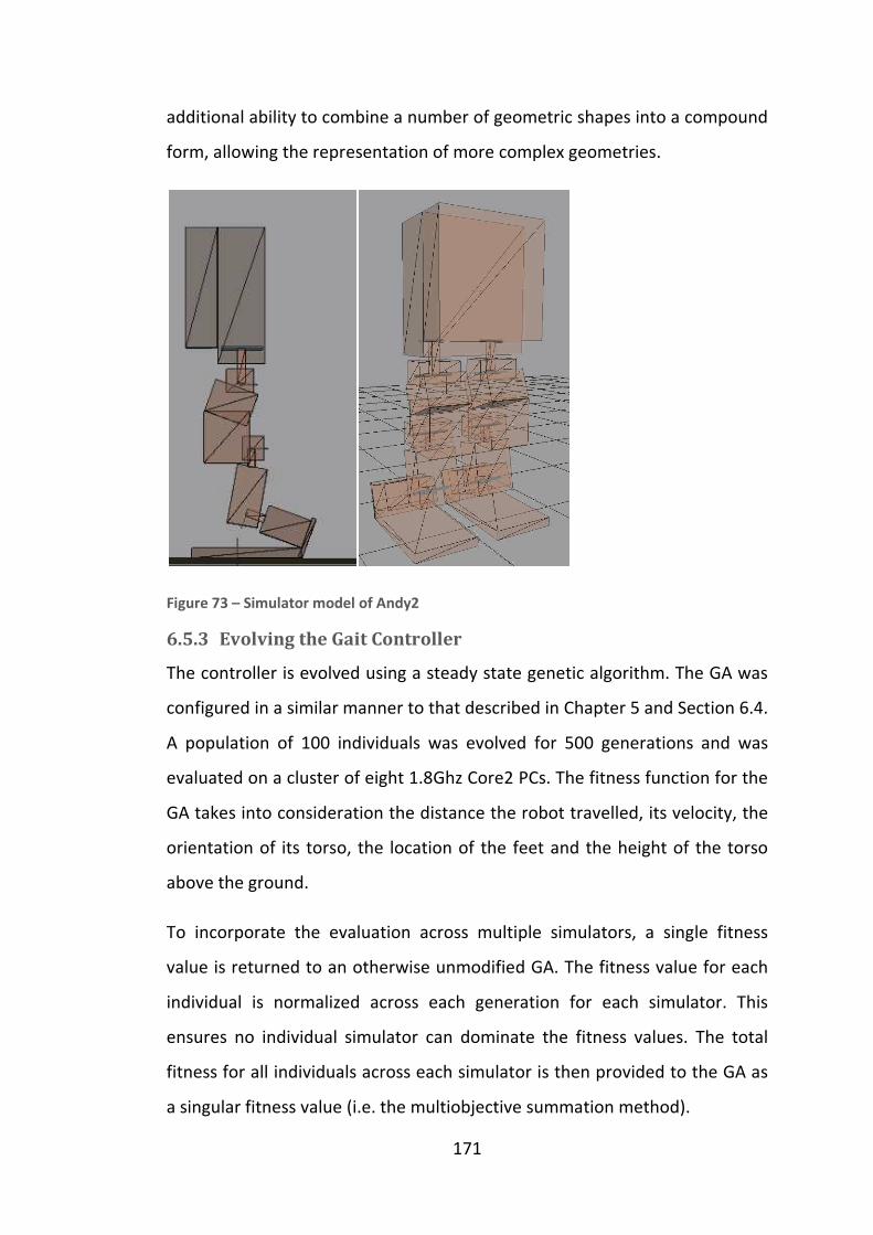
171

additional ability to combine a number of geometric shapes into a compound

form, allowing the representation of more complex geometries.

Figure 73 – Simulator model of Andy2

6.5.3 Evolving the Gait Controller

The controller is evolved using a steady state genetic algorithm. The GA was

configured in a similar manner to that described in Chapter 5 and Section 6.4.

A population of 100 individuals was evolved for 500 generations and was

evaluated on a cluster of eight 1.8Ghz Core2 PCs. The fitness function for the

GA takes into consideration the distance the robot travelled, its velocity, the

orientation of its torso, the location of the feet and the height of the torso

above the ground.

To incorporate the evaluation across multiple simulators, a single fitness

value is returned to an otherwise unmodified GA. The fitness value for each

individual is normalized across each generation for each simulator. This

ensures no individual simulator can dominate the fitness values. The total

fitness for all individuals across each simulator is then provided to the GA as

a singular fitness value (i.e. the multiobjective summation method).

Any individual that is prematurely terminated in one simulator is then given a

zero total fitness score, and the individual is not evaluated on any additional

simulation systems. The Pareto

illustrated in Figure 74. Any terminated individual is given a zero fitness

value, and otherwise is given the sum of its simulator fitness scores. The

arrow indicates the individuals that perform best, on average, across both

simulators. These are likely to be the most robust solutions.

Figure 74 – The fitness evaluation for multiple simulators

The generic process for multi

introduction as:


2. Evaluate each design in

3. Use statistical methods to assign a fitness value indicating how well


4. Use an evolutionary algorithm to

designs

5. Return to Step 2, unless the task is solved

for all of the simulators

172



Pareto efficiency for a system with two simulators is

. Any terminated individual is given a zero fitness


iduals that perform best, on average, across both

simulators. These are likely to be the most robust solutions.

The fitness evaluation for multiple simulators

The generic process for multi-simulator evolution was given in the

Initialize a set of potential controller designs

Evaluate each design in a set of simulators

methods to assign a fitness value indicating how well


Use an evolutionary algorithm to generate a new set of controller

Return to Step 2, unless the task is solved within a confidence interval

all of the simulators



for a system with two simulators is

. Any terminated individual is given a zero fitness


iduals that perform best, on average, across both

n in the

methods to assign a fitness value indicating how well

generate a new set of controller

within a confidence interval,

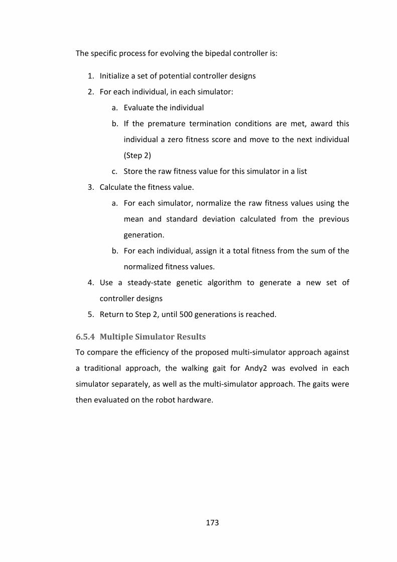
173

The specific process for evolving the bipedal controller is:


2. For each individual, in each simulator:

a. Evaluate the individual

b. If the premature termination conditions are met, award this

individual a zero fitness score and move to the next individual

(Step 2)

c. Store the raw fitness value for this simulator in a list

3. Calculate the fitness value.

a. For each simulator, normalize the raw fitness values using the

mean and standard deviation calculated from the previous

generation.

b. For each individual, assign it a total fitness from the sum of the

normalized fitness values.

4. Use a steady-state genetic algorithm to generate a new set of

controller designs

5. Return to Step 2, until 500 generations is reached.

6.5.4 Multiple Simulator Results

To compare the efficiency of the proposed multi-simulator approach against

a traditional approach, the walking gait for Andy2 was evolved in each

simulator separately, as well as the multi-simulator approach. The gaits were

then evaluated on the robot hardware.

174

Figure 75 – Highest fitness individual per generation for four separate runs of a single

simulator

Figure 75 depicts the raw highest fitness for the new individuals in each

generation. Four separate evolution runs are illustrated for two different

physics engines. The fitness score is a raw score from the fitness function and

has not been normalized. This figure illustrates the need for the statistical

normalization of the fitness scores. The Novodex physics engine consistently

allowed a higher scoring individual, whereas the ODE physics engine typically

scored the lowest. If the fitness values were summed without a

normalization process, then the Novodex evaluated gait would have a higher

contribution to the overall fitness of the individual. Since there is no way of

knowing which physics engine provides the most accurate representation of

reality, each must be weighted evenly. By normalizing the scores each

engines average contribution will be identical.

0

2

4

6

8

10

12

1 51 101 151 201 251 301 351 401 451

Ra

w F

itn

ess

Generation

Best Individual per Generation

Novodex (1)

Novodex (2)

ODE (1)

ODE (2)

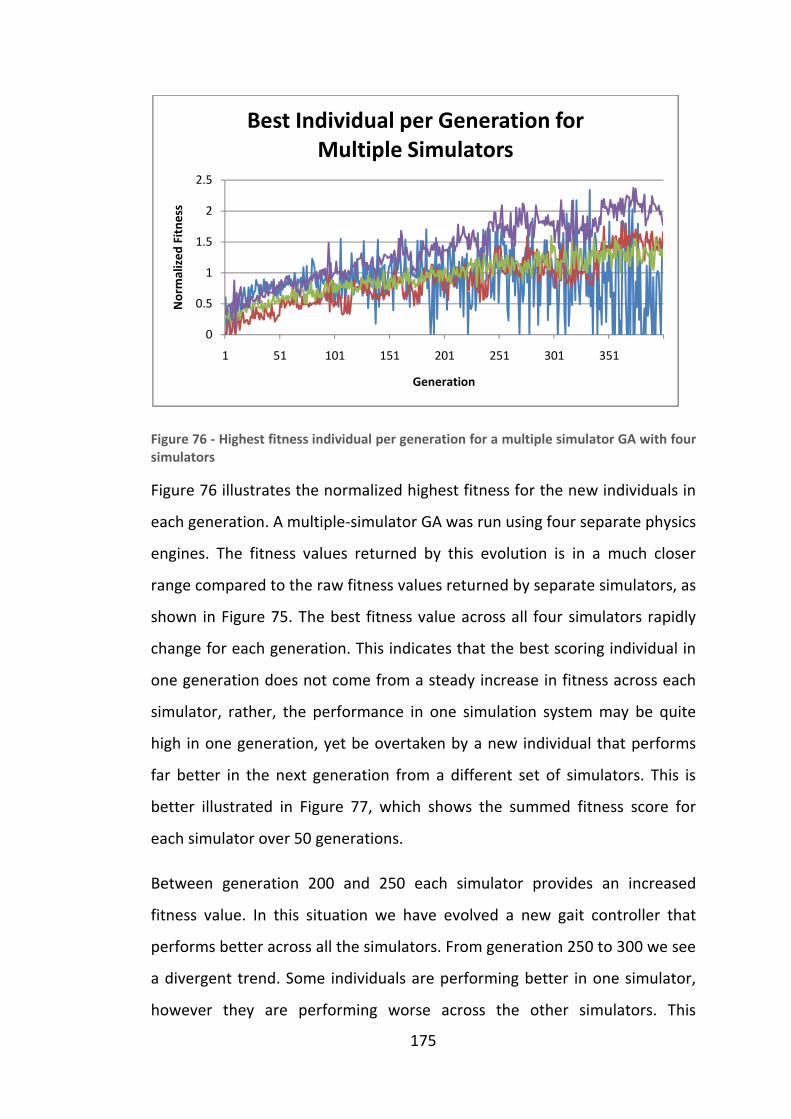
175

Figure 76 - Highest fitness individual per generation for a multiple simulator GA with four

simulators

Figure 76 illustrates the normalized highest fitness for the new individuals in

each generation. A multiple-simulator GA was run using four separate physics

engines. The fitness values returned by this evolution is in a much closer

range compared to the raw fitness values returned by separate simulators, as

shown in Figure 75. The best fitness value across all four simulators rapidly

change for each generation. This indicates that the best scoring individual in

one generation does not come from a steady increase in fitness across each

simulator, rather, the performance in one simulation system may be quite

high in one generation, yet be overtaken by a new individual that performs

far better in the next generation from a different set of simulators. This is

better illustrated in Figure 77, which shows the summed fitness score for

each simulator over 50 generations.

Between generation 200 and 250 each simulator provides an increased

fitness value. In this situation we have evolved a new gait controller that

performs better across all the simulators. From generation 250 to 300 we see

a divergent trend. Some individuals are performing better in one simulator,

however they are performing worse across the other simulators. This

0

0.5

1

1.5

2

2.5

1 51 101 151 201 251 301 351

No

rma

lize

d F

itn

ess

Generation

Best Individual per Generation for

Multiple Simulators

176

situation illustrates how one simulator can provide what seem to be good

results, however these gaits will perform poorly in other simulators and

hence are likely to perform poorly in the real world.

In generation 350 there is a different divergent trend, in that three of the

simulators have an increased fitness value for the controller, whereas one

simulator has a decreased fitness value. In this situation there are three

possibilities. First, that the poorly performing simulator does not have an

accurate representation of the physical reality, and hence provides a

different (worse) fitness value. Second, that three of the simulators share

some common assumptions regarding their configuration (e.g. collision

detection algorithm) and hence provide similar performance benefits from

certain simulator optimizations. Finally, it is possible that both the first and

second case are combined. That is, one of the simulators is employing an

inappropriate simulation technique which is not representative of the real

world. Without verifying the evolved control programs on the real hardware

for each generation, there is no method for determining which simulator is

providing the best representation of the physical reality.

Figure 77 – Summed fitness score over 50 generations for the multi-simulator GA

0

20

40

60

80

100

120

200 220 240 260 280 300 320 340

Su

mm

ed

Fit

ne

ss

Generation

Best Individual Fitness Sum

177

Overall, this indicates there is no single ideal solution that will provide an

increased fitness for all simulators, and that it cannot be assumed that one

individual simulator will provide the most accurate representation of reality.

An example of the GA’s overall performance for the multi-simulator

configuration is given in Figure 78 and the single simulator configuration in

Figure 79. These figures show the normalized fitness scores relative to the

initial generation. These figures are typical of all the results generated for the

evolution runs. The actual performance of the genetic algorithm itself is not

influenced by introducing the multi-simulator technique. At the termination

of the GA, all the evolved populations had converged.

Figure 78 – The GA performance for the multi-simulator configuration

0

0.2

0.4

0.6

0.8

1

1.2

1.4

1.6

1.8

1 51 101 151 201 251 301 351 401 451

No

rma

lize

d F

itn

ess

Generation

GA Evolution for Multi-Simulator

Average

Best

Worst

178

Figure 79 – The GA performance for the single simulator configuration

Each GA run would typically evaluate between 10,000 and 15,000 individuals.

From the collection of over 40,000 datapoints of the execution of the entire

multi-simulator GA, a probability distribution of the individuals fitness values

was generated. The fitness values were normalized against the initial

population. On average, 11.6% of individuals met the termination conditions

and were not evaluated to their full extent. The majority of individuals

produced a relatively poor fitness value of 0.1 standard deviations higher

from the initial generation. Only 7% of the individuals generated managed to

score a fitness value over 1 standard deviation above the distribution in the

original generation.

0

0.2

0.4

0.6

0.8

1

1.2

1.4

1.6

1.8

2

1 51 101 151 201 251 301 351 401 451

No

rma

lize

d F

itn

ess

Generation

GA Evolution for Single Simulator

Average

Best

Worst

Figure 80 – Probability distribution of the fitness value range

From this data we can extract the additional computation load required to

evaluate each extra simulator. Adding an additional simulat

traditional single-simulator approach increases the computation time

required by a factor of 1.8 (N=2). Evaluating four additional simulators (N=5)

requires approximately four and a half times the computation time of

evaluating just a single simu

according to the time required to evaluate each simulator on the target

hardware. For example, one simulator may be optimized for a particular

platform and thus have a lower computation requirement than othe

simulators. Figure 81

computation time to evaluate each individual. Overall, the computation time

for the multisimulator approach was under one fifth of the computation time

required for the high fidelity simulator approach.

179

Probability distribution of the fitness value range


evaluate each extra simulator. Adding an additional simulat

simulator approach increases the computation time



evaluating just a single simulator. The exact computation times may also vary



platform and thus have a lower computation requirement than othe

81 assumes that the simulators require a similar amount of


tisimulator approach was under one fifth of the computation time

required for the high fidelity simulator approach.


evaluate each extra simulator. Adding an additional simulator to the

simulator approach increases the computation time



lator. The exact computation times may also vary



platform and thus have a lower computation requirement than other

assumes that the simulators require a similar amount of


tisimulator approach was under one fifth of the computation time

Figure 81 – Extra computation time for evaluating additional simulators

6.5.4.1 Resultant Gaits

The multi-simulator approach produced successful walking gaits for every

evolution attempted. Every gait successfully transferred to the real robot

hardware to produce a walking robot behaviour. This was not always the

case with the controllers evolved with only a single simulato

Figure 82 – Robot footprints for a gait evolved with multiple simulators (left to right)

180

Extra computation time for evaluating additional simulators

oach produced successful walking gaits for every



case with the controllers evolved with only a single simulator.

Robot footprints for a gait evolved with multiple simulators (left to right)

oach produced successful walking gaits for every



Robot footprints for a gait evolved with multiple simulators (left to right)

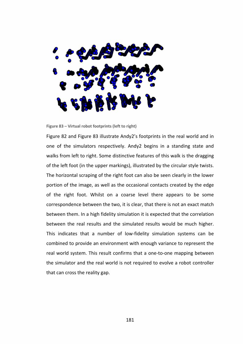
Figure 83 – Virtual robot footprints (left to right)

Figure 82 and Figure

one of the simulators respective

walks from left to right. Some distinctive features of this walk is the dragging

of the left foot (in the upper markings), illustrated by the circular style twists.

The horizontal scraping of the right foot can also

portion of the image, as well as the occasional contacts created by the edge

of the right foot. Whilst on a coarse level there appears to be some

correspondence between the two, it is clear, that there is not an exact match

between them. In a high fidelity simulation it is expected that the correlation

between the real results and the simulated results would be much higher.

This indicates that a number of low

combined to provide an environment

real world system. This result confirms that a one

the simulator and the real world is not required to evolve a robot controller

that can cross the reality gap.

181

Virtual robot footprints (left to right)

Figure 83 illustrate Andy2’s footprints in the real world and in

one of the simulators respectively. Andy2 begins in a standing state and



The horizontal scraping of the right foot can also be seen clearly in the lower




tween them. In a high fidelity simulation it is expected that the correlation


This indicates that a number of low-fidelity simulation systems can be

combined to provide an environment with enough variance to represent the

real world system. This result confirms that a one-to-one mapping between



illustrate Andy2’s footprints in the real world and in

ly. Andy2 begins in a standing state and



be seen clearly in the lower




tween them. In a high fidelity simulation it is expected that the correlation


fidelity simulation systems can be

with enough variance to represent the

one mapping between


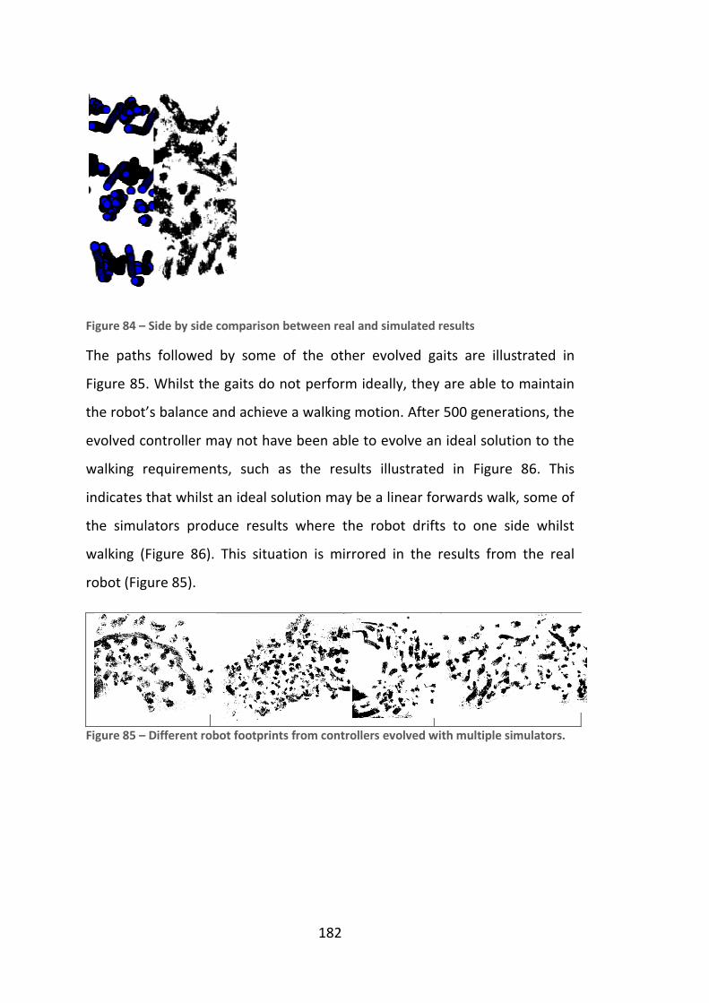
Figure 84 – Side by side comparison between real and simulated results

The paths followed by some of the other evolved gaits are illustrated in

Figure 85. Whilst the gaits do not perform ideally, they are able to maintain

the robot’s balance and achieve a walking motion. After 500 generations, the

evolved controller may not have been able to evolve an ideal solution to the

walking requirements, such as the

indicates that whilst an ideal solution may be a linear forwards walk, some of

the simulators produce results where the robot d

walking (Figure 86). This situation is mirrored in the results from the real

robot (Figure 85).

Figure 85 – Different robot footprints from controllers evolved with multiple simulators.

182

Side by side comparison between real and simulated results


. Whilst the gaits do not perform ideally, they are able to maintain



walking requirements, such as the results illustrated in Figure


the simulators produce results where the robot drifts to one side whilst

). This situation is mirrored in the results from the real

Different robot footprints from controllers evolved with multiple simulators.


. Whilst the gaits do not perform ideally, they are able to maintain



Figure 86. This


rifts to one side whilst

). This situation is mirrored in the results from the real

Different robot footprints from controllers evolved with multiple simulators.

Figure 86 – The foot-ground contact positions for four differ

top)

Figure 87 – Foot-ground contact points for a robot controller evolved in only one

simulator (left to right). The transferred simulator foot

in red.

Figure 87 illustrates the contact points generated from a robot controller

evolved in a single target simulator (indicated in blue). The red points

indicate the contac

transferred into another simulator. This illustrates that two simulation

systems with an identical configuration can produce results that are vastly

different (i.e. the robot walks in one simulator (b

other (red)). This controller was then evaluated on the real robot. The real

robot produced contact results similar to those from the transferred

simulator (e.g. compare

in Figure 88, and are typical results for most of the controllers evolved in a

single simulator.

183

ground contact positions for four different simulators (bottom to

ground contact points for a robot controller evolved in only one

simulator (left to right). The transferred simulator foot-ground contact points are shown

illustrates the contact points generated from a robot controller


indicate the contact points generated by the same robot controller that is



different (i.e. the robot walks in one simulator (blue) but falls over in the



simulator (e.g. compare Figure 87 and Figure 88). These results are depicted

, and are typical results for most of the controllers evolved in a

ent simulators (bottom to

ground contact points for a robot controller evolved in only one

ground contact points are shown

illustrates the contact points generated from a robot controller


t points generated by the same robot controller that is



lue) but falls over in the



). These results are depicted

, and are typical results for most of the controllers evolved in a

Figure 88 – Robot footprints for a single simulator target evolution

Figure 89 shows the height of the torso above ground during a 10 second

walking simulation. The target simulator maintains a steady walk with the

torso height remaining near the

simulator the torso’s position drops at around 5 seconds, implying that the

robot maintains a walk for a short period and then the robot falls to the

ground. The data from the torso’s displacement from its de

(Figure 90) shows that the robot does not actually walk, but rather rocks

from side to side on the spot before falling. This does not correspond with

the results from the real robot’s walk, where it attempted a step and fell.

This indicates that none of the individual simulators provided an accurate

representation of what happened in the real world.

Figure 89 – Torso height variation for a single simulation target

184

Robot footprints for a single simulator target evolution

shows the height of the torso above ground during a 10 second


torso height remaining near the original standing position. In the transferred



ground. The data from the torso’s displacement from its desired position

) shows that the robot does not actually walk, but rather rocks


e results from the real robot’s walk, where it attempted a step and fell.


representation of what happened in the real world.

ation for a single simulation target

shows the height of the torso above ground during a 10 second


original standing position. In the transferred



sired position

) shows that the robot does not actually walk, but rather rocks


e results from the real robot’s walk, where it attempted a step and fell.


Figure 90 – Torso displacement from the desired walking position

The overall walking performance of the eight gaits evolved for the single and

multiple simulator approaches is presented in

more than 10 steps was deemed to have a stable walk, so data was not

collected beyond this point. Overall only two of the controllers evolv

a single simulator managed to cross the reality gap. Of these two, one only

sometimes managed to take a half a single step before falling and so its

partial success is considered pure luck. The other successful gait was evolved

with the ODE physics

Chapter 4), however it failed to produce this result with a second evolved

gait. Although this would indicate that controllers evolved with the ODE

simulator have a high chance of crossing the reality

results from the high fidelity simulator (N=4) indicate that it is unlikely that it

would reliably cross the reality gap every time. For all other simulators, none

of them managed to cross the reality gap, and as indicated by the result

Figure 87, none would successfully transfer from one simulator to another.

Every gait controller evolved with multiple simulators successfully

transferred to the real robot, confirming the hypothesis that using multiple

simulators will improve the validity of the robot simulations. Six of the eight

185

Torso displacement from the desired walking position


multiple simulator approaches is presented in Figure 91. Any robot managing


collected beyond this point. Overall only two of the controllers evolv




with the ODE physics engine which has high quality constraint solvers (See



simulator have a high chance of crossing the reality gap (50%, N=2), the



of them managed to cross the reality gap, and as indicated by the result

, none would successfully transfer from one simulator to another.


e real robot, confirming the hypothesis that using multiple



. Any robot managing


collected beyond this point. Overall only two of the controllers evolved from




engine which has high quality constraint solvers (See



gap (50%, N=2), the



of them managed to cross the reality gap, and as indicated by the results in

, none would successfully transfer from one simulator to another.


e real robot, confirming the hypothesis that using multiple


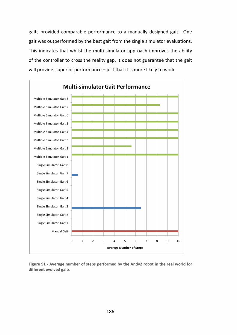
186

gaits provided comparable performance to a manually designed gait. One

gait was outperformed by the best gait from the single simulator evaluations.

This indicates that whilst the multi-simulator approach improves the ability

of the controller to cross the reality gap, it does not guarantee that the gait

will provide superior performance – just that it is more likely to work.

Figure 91 - Average number of steps performed by the Andy2 robot in the real world for

different evolved gaits

0 1 2 3 4 5 6 7 8 9 10

Manual Gait

Single Simulator Gait 1








Multiple Simulator Gait 1








Average Number of Steps

Multi-simulator Gait Performance

187

6.6 Bipedal Robot Control Summary

The results from the walking robot simulation have a number of implications.

Automatically evolved control programs that managed to successfully cross

the reality gap demonstrate that these approaches work for mechanically

complex robots without requiring any hardware in the loop. This was

demonstrated for both the high fidelity approach and the multiple simulator

approach.

Traditional high fidelity simulations provided an acceptable solution to

evolving gaits, however it required a highly accurate model of the robot,

significant computational effort, and still did not always successfully cross the

reality gap. The high fidelity simulators provided a relatively close mapping

between the simulator and the real world. This was not the case for the

multi-simulator approach. These results demonstrate that it is not necessary

to have a simulator that provides an exact representation of reality. Multiple

low fidelity simulators can be leveraged to evolve robust robot controllers


The fitness results from the multi-simulator genetic algorithm indicate that

there are two major classes of controller solutions:

1. Controllers that perform well in a subset of simulators. This

includes controllers that perform well in only a single simulator and

controllers that perform well in all but one simulator.

2. Controllers that perform well in all simulators.

The data from evaluating controllers evolved with a single low-fidelity

simulator indicates that none of the individual simulators was able to

produce a reliable representation of the real world robot. This implies that

the first class of controllers did not include controllers that were robust

enough to successfully cross the reality gap.

188

The controllers evolved with multiple simulators, which also performed well

in all the simulators, managed to cross the reality gap and produce a stable

walking gait on the real robot. This implies that the combination of the

simulators different algorithms provides a valid model for evolving a robust

robot controller. Furthermore, the results from these experiments indicate

that the multiple simulator approach produces more reliable results than the

high fidelity simulation approach.

None of the simulators used provided a perfectly accurate model of the real

world. This adds weight to Brook’s argument that it is not possible to

construct a highly accurate dynamics simulator of the real world. The results

in this chapter suggest that the dynamics problem of the reality gap can be

overcome by leveraging multiple simulation systems in the design of a

robot’s control system.

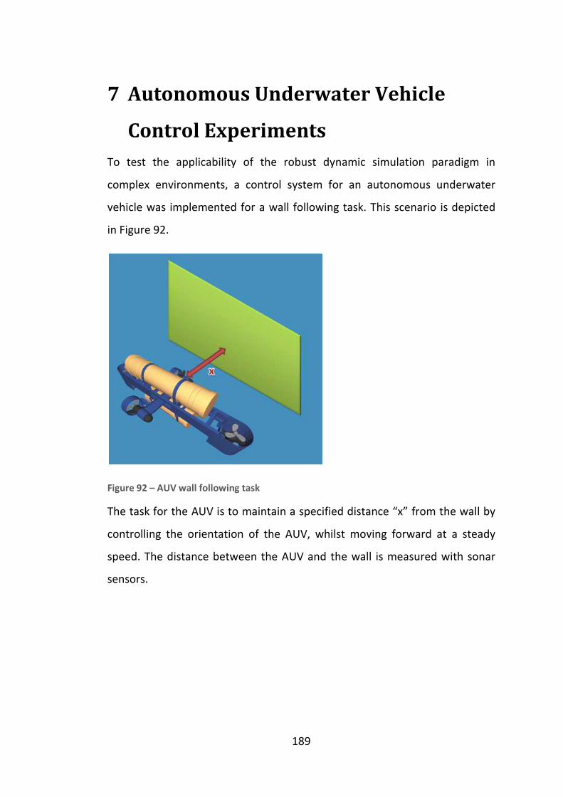
7 Autonomous Underwater Vehicle

Control Experiments

To test the applicability of the robust dynamic simulation paradigm in

complex environments, a control system for an autonomous underwater

vehicle was implemented for a wall following task. This scenario is depicted

in Figure 92.

Figure 92 – AUV wall following task

The task for the AUV is to maintain a specified distance “x” from the wall by

controlling the orientation of the AUV, whilst mo

speed. The distance between the AUV and the wall is measured with sonar

sensors.

189

Autonomous Underwater Vehicle

Control Experiments




AUV wall following task


controlling the orientation of the AUV, whilst moving forward at a steady


Autonomous Underwater Vehicle





ving forward at a steady


190

7.1 Physical Simulation Problems for Robots in

Fluids

Modelling the behaviour of fluids interacting with an underwater robot poses

a number of difficulties. Simulated fluids are deterministic chaotic systems

(106). In an SPH simulation, if the initial position of the particles is slightly

altered, the movement of a body through the fluid may cause the resultant

state of the liquid to be significantly different. This is an accumulation of the

effect of the contributions of each particle to the liquid forces and the

particle integration effects. These factors can be strongly influenced by a

particular physics engine collision detection and response system. As a result,

the collision shape of the robot moving through the liquid can have a large

influence on the simulation state.

SPH methods are also computationally intensive, resulting in a practical limit

in the size of the liquid body that can be effectively simulated. This limits the

application of SPH fluids to smaller bodies of liquid. Finally, determining the

correct parameter settings for configuring an SPH simulation is not a trivial

matter, and it is often difficult to create a stable simulation of the properties

of real water.

Grid based approaches, such as dampened shallow waves, also suffer from

similar chaotic behaviour to particle based methods. Shallow wave

approaches are less computationally intensive than particle based

approaches, however they cannot simulate splashing and suffer from aliasing

issues from having a grid applied over the geometry in the simulated

environment (135).

191

Figure 93 – Collision boundaries for Eulerian and Lagrangian fluid representations

Simulating fluid effects directly onto rigid bodies has the advantage of being

computationally cheap, allowing the simulation of large bodies of water.

Determining the correct parameters for simulating water is simpler than SPH

based methods. This simplifies the creation of realistic and accurate

simulations. The interaction between a fluid and other bodies cannot be

simulated and thus the method may not provide fully accurate results when

a body is in the vicinity of an environmental obstacle (for example, when the

AUV is near the wall).

Figure 93 illustrates how collision boundaries are handled in Eulerian (135)

(e.g. Shallow Wave Equations) and Lagrangian (135) (e.g. Smoothed Particle

Hydrodynamics) based approaches. The direct simulation approach applies

drag and lift forces directly on the body without consideration to the fluid

structure and does not model boundaries at all. The left side of the Figure

depicts the aliasing problem that occurs with grid-based approaches.

Lagrangian approaches do not have this problem as the particles move and

respond to the object boundaries.

Smoothed Particle Hydrodynamics simulation stability and accuracy is a

function of the smoothing kernels used (135). Regardless of the kernel

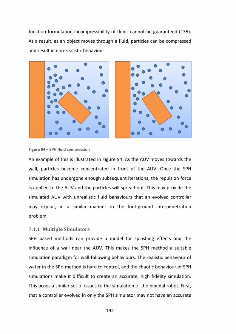
192

function formulation incompressibility of fluids cannot be guaranteed (135).

As a result, as an object moves through a fluid, particles can be compressed

and result in non-realistic behaviour.

Figure 94 – SPH fluid compression

An example of this is illustrated in Figure 94. As the AUV moves towards the

wall, particles become concentrated in front of the AUV. Once the SPH

simulation has undergone enough subsequent iterations, the repulsion force

is applied to the AUV and the particles will spread out. This may provide the

simulated AUV with unrealistic fluid behaviours that an evolved controller

may exploit, in a similar manner to the foot-ground interpenetration

problem.

7.1.1 Multiple Simulators

SPH based methods can provide a model for splashing effects and the

influence of a wall near the AUV. This makes the SPH method a suitable

simulation paradigm for wall-following behaviours. The realistic behaviour of

water in the SPH method is hard to control, and the chaotic behaviour of SPH

simulations make it difficult to create an accurate, high fidelity simulation.

This poses a similar set of issues to the simulation of the bipedal robot. First,

that a controller evolved in only the SPH simulator may not have an accurate

193

enough representation of reality in order to cross the reality gap. Second, the

evolutionary algorithm may find and optimize specific controllers that take

advantage of putting the SPH liquid into a specific state. Much like the foot-

ground interpenetration problem, SPH particles may also be forced into an

unstable interpenetration state, resulting in an unrealistic force being applied

to the submersed body. This would result in the controller becoming

dependent on the unrealistic behaviour of the fluid.

Coupling the SPH simulation with another simulation that directly calculates

the fluid effect contributions eliminates the possibility of a controller

becoming dependent on unrealistic fluid particle states. Furthermore, as was

the case with the bipedal robot simulation, the extra simulator may provide

an additional means for increasing the robustness of the resulting controller.

7.2 AUV Hardware and Simulation Software

The Mako AUV is a two-hull, four-thruster configuration, it measures 1.34 m

long, 64.5 cm wide and 46 cm tall. The vehicle comprises two watertight hulls

machined from PVC separately mounted to a supporting aluminium skeletal

frame. Two thrusters are mounted on the port and starboard sides of the

vehicle for longitudinal movement, while two others are mounted vertically

on the bow and stern for depth control (107).

Figure 95 – Mako AUV

194

Propulsion is provided by four modified 12V, 7A trolling motors that allow

horizontal and vertical movement of the vehicle. The starboard and port

motors provide both forward and reverse movement, while the stern and

bow motors provide depth control in both downward and upward directions.

Roll and pitch are passively controlled by the vehicle’s innate righting

moment, though pitch can be controlled by the stern and bow motors if

necessary. Lateral movement is not possible for the vehicle, however, this

ability is not necessary, as the starboard and port motors allow yaw control

which permits movement in any global horizontal direction. Overall, this

provides the vehicle with 4DOF that can be actively controlled (107).

The control system of the Mako is separated into two controllers; an Eyebot

microcontroller and a mini-itx PC running Linux. The Eyebot controller runs at

33MHz and comprises 512K of ROM, as well as 2048K of RAM. This

controller’s primary purpose is in controlling the four thrusters, that is,

controlling the vehicle’s movement and the AUV’s sensors. The mini PC

comprises a Cyrix 233MHz processor, 32Mb of RAM and a 5GB hard drive. Its

function is to provide processing power for the computationally intensive

vision system (107).

The sensor system is custom-made using four 200kHz Navman Depth 2100

transducer and the LM1812 ultrasonic transceiver chip. The sensors are

placed on the bow, port and starboard sides of the AUV and are used to

determine the proximity of obstacles to the AUV. One sensor is pointing

directly down for depth sensing. A low-cost Vector 2X digital magnetic

compass module provides for yaw or heading control.

7.2.1 SubSim: An AUV Simulator

SubSim is a real-time submersible vehicle simulation package (136). The

physical motion of the submarine is calculated using the Physics Abstraction

Layer (See Chapter 3). The package provides a low level controller simulation

interface that enables developers to build a simulation of their own control

system environments.

customized such that SubSim’s interface mirrors the interface of the real

controller.

The high level of customizability of the package enables simulation of very

specific tasks as well as general operatio

tool for testing AUV design and control.

The simulation software is designed to address a broad variety of users with

different needs, such as the structure of the user interface, levels of

abstraction, and the complexity

the most important design goal for the software is to produce a simulation

tool that is as extensible and flexible as possible.

A component plug-

for a wide range of operations. The interoperation of the different modules

of SubSim is illustrated in

SubSim’s operation.

Figure 96 – SubSim software design

195


system environments. The graphical user interface is modular and can be



specific tasks as well as general operation. This makes SubSim an excellent

tool for testing AUV design and control.



abstraction, and the complexity of physical and sensor models. As a result,


tool that is as extensible and flexible as possible.

in architecture allows users to modify SubSim’s behaviour

de range of operations. The interoperation of the different modules

of SubSim is illustrated in Figure 96. There are five major stages that define

SubSim’s operation.

SubSim software design


The graphical user interface is modular and can be



n. This makes SubSim an excellent



of physical and sensor models. As a result,


in architecture allows users to modify SubSim’s behaviour

de range of operations. The interoperation of the different modules

. There are five major stages that define

196

The lowest layer is the XML parser, which reads the configuration files, and

the physics engine. The physics engine is responsible for maintaining the low

level details on the state of the rigid bodies in the simulated environment.

This includes properties such as a body’s mass, position, orientation, and the

forces and torques acting on the body. The physics engine also maintains the

collision information for the environment and determines how objects

behave after a collision occurs.

The Physics Abstraction Layer library lies on top of the physics engine and

provides the interchangeable low level physics engine capabilities, as well as

providing the higher level physics simulation attributes, such as the

propulsion system and sensor models. Low level error modelling is also

implemented at this layer.

Next sits the simulation core and graphics engine. The graphics engine is

responsible for displaying the visual 3D data to the user, as well as simulating

the camera sensor. The simulation core performs all the application specific

tasks and provides the interface for allowing user programs to interact with

the virtual vehicle and the virtual world. Higher level error models and

controller simulation is performed in this layer.

The last layer of the SubSim package is the user interface. All the controls

presented to the user are present at this stage. This includes information

displays, such as sensor readings and state information, as well as the visual

interface for interacting with the vehicles control systems.

Finally, the user program that controls the vehicle’s actions for the simulation

interacts with the simulation core, simulated controller, and UI to perform

the desired tasks. This is achieved through the use of two APIs exposed by

SubSim. The first API is the internal API, which is exposed to developers, so

that they can encapsulate the functionality of their own controller API. The

197

second API is the RoBIOS API (65), a user friendly API that mirrors the

functionality present on the Eyebot controller found on the Mako.

Plug-in capabilities are available at every stage of SubSim. The physical

simulation of the vehicle can be completely customized by interchanging the

low-level physics engine and collision system with a different existing engine.

The high-level physical simulation behaviour, such as the actuator and sensor

models, can be modified via the PAL plug-ins. Error models for the simulation

of the actuators and sensors can be performed with both the PAL plug-ins

and the simulation core plug-ins.

Simulation of custom controllers and associated devices can be performed by

creating plug-ins for the simulation core. User interface plug ins are available

to provide a graphical interface to any additional plug ins (e.g. a simulated

controller) or to extend the functionality of the SubSim package itself.

Providing pluggable component interfaces at each major level of SubSim’s

operation is what makes SubSim such a versatile, flexible and extensible tool.

7.2.2 SubSim Environment

The terrain is an essential part of the environment as it defines the universe

the simulation takes part in, as well as physical obstacles the AUV may

encounter. SubSim can simulate height map environments, a data format

typically found from geological surveys. SubSim also supports models

produced by 3D CAD packages. This allows interaction with a complex

simulated environment, such as oilrigs and pipelines fixed to the ocean floor.

Whilst the terrain is in a fixed position and its properties cannot be

influenced by an interacting object or vehicle, environmental objects such as

buoys or pipes can be influenced by the interacting vehicles. This allows

simulation of autonomous vehicles that can modify their environment in

addition to underwater vehicles designed for inspection purposes.

198

Environmental effects, such as lighting conditions and water currents are also

possible. These dynamic conditions allow for the modelling of more complex

behaviour, e.g. introducing (ocean) currents causes the submarine to

permanently adapt its position, poor lighting and visibility decreases image

quality and eventually adds noise to PSD and vision sensors.

Figure 97 – SubSim application screen shot

7.3 Evolving an AUV Wall Following Controller

7.3.1 PID Control Algorithm

A PID controller was employed to maintain a one meter distance from the

left wall. Initially, the sonar sensor is read to obtain the distance from the

wall. If the sonar reading is too large then it is assumed to be a faulty reading.

The error between the measured distance and the desired distance is then

provided to the PID controller, and the left and right motor speeds are set

199

relative to a normal speed and clamped within a valid range. The control

algorithm is present in pseudo code in Listing 3.

while (true): //read sonar do dist = read sonar while dist>30 //do pid speed = PID(dist - 1,dt) //right motor right_speed = motor_speed+speed right_speed = clamp(right_speed,1,-1) drive_starboard(right_speed) //left motor left_speed = motor_speed-speed left_speed = clamp(left_speed,1,-1) drive_portside(left_speed) Listing 3 – Wall following pseudo code

7.3.2 Evolving the AUV Control System

To evolve the control system the PID parameters were encoded into three 16

bit fixed point values with a valid range of -1 to 1. A genetic algorithm was

used to evolve the controller. The GA was configured to use a fitness

proportionate selection scheme with elitism. Only two genetic operators

were employed, a bitwise crossover and a bitwise mutate. The crossover

operator was selected 90% of the time and mutation the remaining 10%. A

population of 40 individuals was evaluated over 50 generations.

The raw fitness function was simply the summed difference between the

desired AUV position and the measured AUV position over time. Thus, the GA

was designed to minimize the fitness value, as the fitness measurement

represented the cumulative error for the control system. To reduce the

computational burden of evaluating inappropriate controllers, any AUV

simulation that came into contact with the wall was terminated and assigned

a poor fitness value.

200

[#$4 = 6 |4[ − #am#|(7

Equation 84 – Fitness function

To eliminate the effects of one simulation system providing consistently

better or worse fitness values for an identical control system, the fitness

functions were normalized relative to the initial population.

$45 = 1 v [#$4T − $µT¶T·

T´7

Where, N is the number of simulation systems evaluated

rawfit is the fitness value from the ith simulation system $µT is the mean fitness value of the initial population of the ith

simulation system

and ¶T is the standard deviation of the fitness of the initial population. Equation 85 – Fitness normalization

A noisy fitness function (108) is not employed, since the variation found

between simulation systems is in fact deterministic (106). A given simulation

system started with identical parameters will always generate the exact same

result (even if slight changes, such as the starting position of one particle of

water may result in different AUV motion results).

A robust fitness function (108) is also not employed, as the variation

provided by the differences in how the dynamic simulation system evaluates

the robot’s locomotion is hypothesized to provide enough variance to

generate a robust control system.

7.4 Evaluation with Multiple Simulation Systems

To demonstrate the variance in fitness achieved by varying the simulator the

position plot for the Mako AUV in the Ageia PhysX dynamics simulator is

shown in Figure 98. The parameters for this PID controller were evolved for a

single non-SPH simulator. The red plot represents the position where the

201

dynamics are calculated with SPH, and blue without. The green plot shows

the position without SPH for the Newton Game Dynamics simulator. This plot

illustrates the large variation possible for a AUV simulated using different

dynamic simulation packages. The variation between packages and

simulation paradigms appears to have a large enough variation to present a

suitable representation of the variation between one simulator and the real

world. This figure clearly shows that a controller evolved using only one

simulation paradigm can completely fail to achieve its goal when transferred

to another simulation paradigm. This mimics the effect found when

transferring a control system evolved in a single paradigm simulator to the

real world.

Figure 98. Motion of the AUV for a controller optimized for one simulation paradigm

AUV Path

PhysX PhysX SPH Newton

202

Figure 99 – Motion of the AUV for a controller evolved with multiple simulation

paradigms

Figure 99 depicts a plot of the position of the AUV for a control system

evolved with multiple simulators. The PID controller can successfully follow

the wall in each simulation paradigm. This indicates that a controller can be

made more robust by evolving it in a multiple paradigm simulation

environment. Unlike the previous control systems evolved in a single

simulator, the control system evolved using both paradigms can successfully

follow the wall and make corrections to its course. The raw fitness functions’

maximum, average and minimum value for the two hydrodynamics

simulation methods are shown in Figure 100.

AUV Path

Non SPH SPH

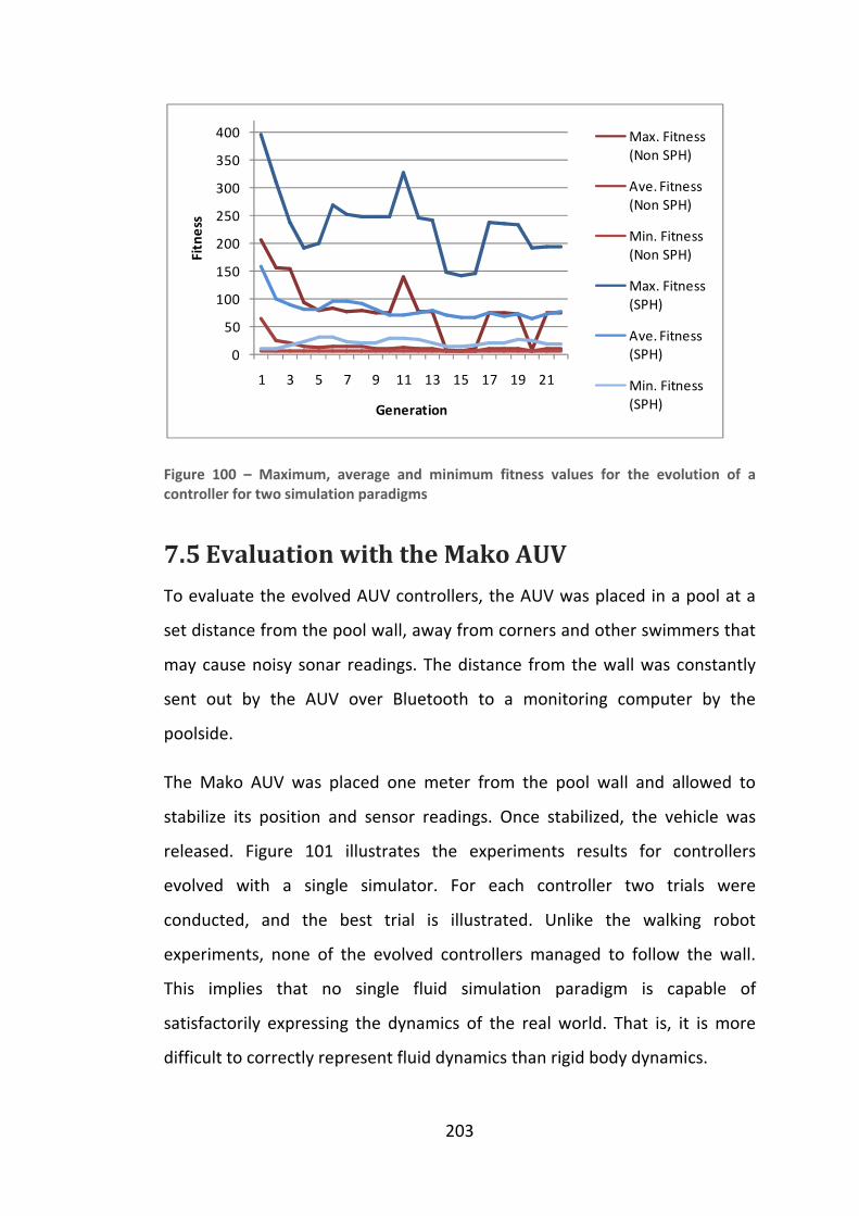
203

Figure 100 – Maximum, average and minimum fitness values for the evolution of a

controller for two simulation paradigms

7.5 Evaluation with the Mako AUV

To evaluate the evolved AUV controllers, the AUV was placed in a pool at a

set distance from the pool wall, away from corners and other swimmers that

may cause noisy sonar readings. The distance from the wall was constantly

sent out by the AUV over Bluetooth to a monitoring computer by the

poolside.

The Mako AUV was placed one meter from the pool wall and allowed to

stabilize its position and sensor readings. Once stabilized, the vehicle was

released. Figure 101 illustrates the experiments results for controllers

evolved with a single simulator. For each controller two trials were

conducted, and the best trial is illustrated. Unlike the walking robot

experiments, none of the evolved controllers managed to follow the wall.

This implies that no single fluid simulation paradigm is capable of

satisfactorily expressing the dynamics of the real world. That is, it is more

difficult to correctly represent fluid dynamics than rigid body dynamics.

0

50

100

150

200

250

300

350

400

1 3 5 7 9 11 13 15 17 19 21

Fit

ne

ss

Generation

Max. Fitness

(Non SPH)

Ave. Fitness

(Non SPH)

Min. Fitness

(Non SPH)

Max. Fitness

(SPH)

Ave. Fitness

(SPH)

Min. Fitness

(SPH)

204

The controller evolved using the direct fluid simulation method in the

Newton Game Dynamics and the PhysX physics engines showed inconsistent

results. For the Newton evolved version the AUV moved towards the wall,

until the sonar sensor read faulty values. The PhysX controller moved away

from its starting position, until it too suffered from faulty sonar readings. The

controller evolved using the SPH simulation paradigm managed to maintain a

distance close to the wall longer than either direct-simulation method, but

also failed. The readings were stopped once the AUV reached the end of the

pool.

Figure 101 – Mako wall following distance readings for a single simulator evolved

controller

The control systems evolved in the multi-paradigm simulation was evaluated

in five trial runs and the distance measurements returned are illustrated in

Figure 102. During the third trial run, the Navman Depth 2100 controller

provided some incorrect readings to the AUV due to other multipath

reflections returning with similar amplitude to the legitimate reflection. This

is illustrated by the break in the graph of Figure 102. Otherwise, the

controller performs well keeping the AUV at a regular distance from the wall.

0

0.5

1

1.5

2

2.5

1 3 5 7 9 11 13 15 17 19 21 23 25 27 29 31 33 35 37 39 41 43 45 47 49 51

Dis

tan

ce f

rom

Wa

ll (

m)

Time (seconds)

Wall following on Mako

Single simulator

PhysX

PhysX - SPH

Newton

205

Some oscillations are visible at the beginning of the plot, but they are not of a

large enough magnitude to cause the AUV to lose the wall.

Figure 102 – Mako wall following distance readings for a multi-paradigm simulator

The resulting plots in Figure 98 and Figure 99 show a strong convergence in

behaviour over the evolution of the control system with and without the SPH

fluid simulation. This demonstrates that it is possible to evolve a single

controller that provides acceptable performance within multiple simulation

systems using different simulation paradigms.

Figure 103 illustrates the maximum error (i.e.: worst fitness) in each

generation. Peaks that coincide with both fluid simulation methods indicate

controllers that performed very poorly, regardless of the simulated

environment (e.g.: hit the wall). Peaks that do not coincide between

simulation systems indicate controllers that performed well with one

simulation method, but not the other.

Both simulation methods are valid approaches for representing the motion

of an object through a fluid, however the fitness peaks which do not coincide

represent a set of controllers that are not robust. That is, they provide a valid

interpretation for a single simulation method, but not both (See Figure 100).

0

0.2

0.4

0.6

0.8

1

1.2

1.4

1 3 5 7 9 11 13 15 17 19 21 23 25 27 29 31 33 35 37

Dis

tan

ce f

rom

Wa

ll (

m)

Time (seconds)

Wall Following on Mako

Multiple Simulators

Tiral 1

Tiral 2

Tiral 3

Tiral 4

Tiral 5

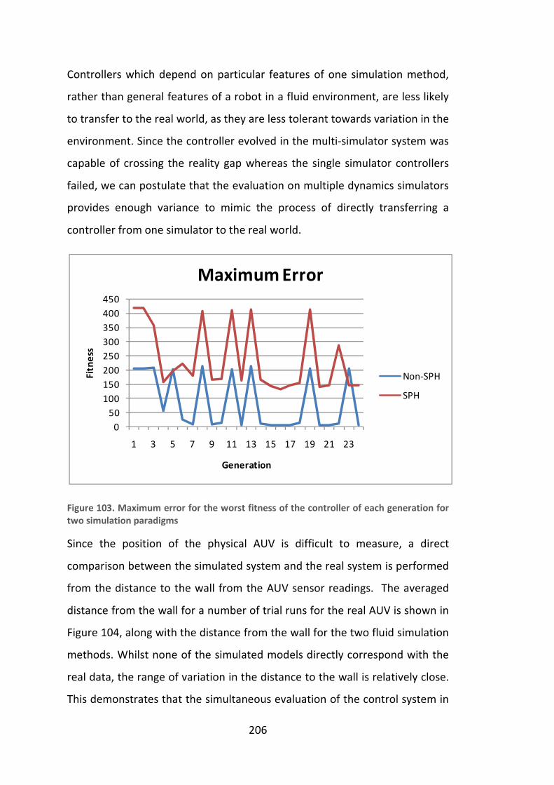
206

Controllers which depend on particular features of one simulation method,

rather than general features of a robot in a fluid environment, are less likely

to transfer to the real world, as they are less tolerant towards variation in the

environment. Since the controller evolved in the multi-simulator system was

capable of crossing the reality gap whereas the single simulator controllers

failed, we can postulate that the evaluation on multiple dynamics simulators

provides enough variance to mimic the process of directly transferring a

controller from one simulator to the real world.

Figure 103. Maximum error for the worst fitness of the controller of each generation for

two simulation paradigms

Since the position of the physical AUV is difficult to measure, a direct

comparison between the simulated system and the real system is performed

from the distance to the wall from the AUV sensor readings. The averaged

distance from the wall for a number of trial runs for the real AUV is shown in

Figure 104, along with the distance from the wall for the two fluid simulation

methods. Whilst none of the simulated models directly correspond with the

real data, the range of variation in the distance to the wall is relatively close.

This demonstrates that the simultaneous evaluation of the control system in

0

50

100

150

200

250

300

350

400

450

1 3 5 7 9 11 13 15 17 19 21 23

Fit

ne

ss

Generation

Maximum Error

Non-SPH

SPH

207

multiple simulation systems is capable of generating a controller that can

cross the reality gap.

Figure 104. Comparison of distance sensor readings for the two simulation paradigms and

the real AUV

7.6 AUV Control Summary

This experiment confirms that the multiple simulator approach is capable of

evolving a robust control system in a simulated environment that can be

directly transferred to a real robot. Furthermore, it demonstrates the

approaches success for robots operating with complex environmental

interactions, and that it is not limited to rigid body systems.

The fitness results from the multi-simulator genetic algorithm indicate that

there are two major classes of controller solutions:

0

0.2

0.4

0.6

0.8

1

0 5 10 15 20 25 30

Dis

tan

ce f

rom

wa

ll (

m)

Time (seconds)

Wall Following - Simulation and

Reality

Non SPH SPH Real AUV

208

1. Controllers that perform well in a subset of simulators. This can be

subdivided into:

a. Controllers that perform well in a single simulator with a single

fluid simulation paradigm

b. Controllers that perform well in multiple simulators with a

single fluid simulation paradigm

2. Controllers that perform well in all simulators. This class consisted

of controllers that performed well in simulators with multiple fluid

simulation paradigms.

From the simulation results, we can determine that controllers evolved in a

single simulator using a single simulation paradigm will perform adequately

in another simulator using the same simulation paradigm. However, the

controller will likely fail in the real world, or if given a different simulation

paradigm. Conversely, controllers evolved using multiple simulation

paradigms would successfully cross the reality gap. The key finding is that

variation in the simulation paradigm (e.g. SPH vs. SWE), is paramount to the

variation in the simulators implementation details (e.g. SPH kernels).

The results from the evaluation on the AUV hardware indicated that

regardless of which single simulation paradigm was chosen, and how

accurately the paradigm modelled the fluid, the AUV would fail to transfer

from simulation to reality. This implies that accurately representing the

dynamics of a fluid is more difficult than representing the dynamics of a rigid

body. Again, agreeing with Brook’s argument that it is not possible to

construct a highly accurate dynamics simulator of the real world.

The results from the controllers evolved across multiple simulation

paradigms proved to be very successful. This indicates that using multiple,

fundamentally different models for representing the simulation can provide a

209

simulation environment enabling control systems to directly transfer from a

simulation to the real world. Furthermore, the success of the multiple

simulator approach for this application indicates that it is a good choice for a

problem where single simulator approaches fail. This result implies that the

optimal simulation configuration for evolving controllers across the reality

gap should contain fundamental differences in how the simulator operates in

order to provide the highest probability of success.

210

8 Conclusion

This thesis presented a new multi-simulator controller evolution paradigm

and the design and implementation of the Physics Abstraction Layer, a

software package which provides a uniform interface to multiple real-time

dynamics simulators. The system was extensively benchmarked and

demonstrated evolving a bipedal robot gait controller and evolving a wall

following program for an autonomous underwater vehicle (AUV). The

properties of different real-time physics engines were investigated and the

performance of different genetic algorithms was analysed.

8.1 Thesis Summary

Chapter 2 discussed a number of physics simulation paradigms for rigid

bodies, soft bodies and fluids. The implementation aspects of different

integrators, time stepping approaches, collision detection, geometry

representations and constraint solvers were discussed. Various paradigms for

fluid simulations were discussed including Eulerian and Lagrangian

approaches. Some of the key differences between the various physics

simulation approaches were addressed.

The Physics Abstraction Layer (PAL), designed and implemented as part of

this thesis, was introduced in Chapter 3. It provides an abstract, generic

interface for modelling and simulating a number of physical systems

including robotic mechanisms. PAL was designed to be easily extensible and

maintain a high level of compatibility between a variety of physics engines. It

also includes a number of tools for importing data from standard CAD

modelling packages. The specific implementation details of the software as

well as various sensor and actuator models were described. This software

211

enabled the extensive benchmarking and controller evolution experiments of

the subsequent chapters.

Chapter 4 included an in-depth benchmark of a number of aspects of modern

physics engines. Integrator, restitution, friction, constraint solvers, stacked

objects, and collision detection routines were extensively benchmarked for

both computational efficiency and physical accuracy with seven different

physics engines. The results were analysed and overall it was found that no

single physics engine excelled in all areas in the tests.

Evolutionary Algorithms (EAs) and control systems were introduced in

Chapter 5. A review of Genetic Algorithms (GAs) covered fitness functions,

selection schemes, genetic operators, chromosome encoding, staged

evolution, premature termination and multi objective optimization. A

simulated walking robot experiment was performed to assess the optimal

configuration of the GA, concluding that staged evolution and early

terminating conditions could significantly reduce the computational

requirements for the GA.

Finally, Chapter 6 and 7 presented some underlying problems of physically

based simulation of two different robot control problems. A gait controller

for a bipedal robot was evolved in three different physics simulation

configurations. First, in a high-fidelity physics simulation system, second in a

standard real-time physics engine and finally using multiple physics engines.

The key problems found when simulating the robot were the foot-ground

interaction and solving the constraint chain.

The results indicated that controllers evolved in high-fidelity simulations

were more likely to cross the reality gap than those that used medium and

low-fidelity simulations. Controllers evolved using multiple low-fidelity

simulations successfully crossed the reality gap and provided more reliable

212

performance than high-fidelity simulations, confirming the hypothesis that

using multiple simulators provides a good representation of the reality gap.

The results also demonstrated that controllers can perform well in one

simulator, but perform poorly in another.

The experiments with the AUV reinforced the results from the bipedal robot

experiments. The simulation problem highlighted for this task was the

simulation of the fluid dynamics in general, and the fluids behaviour near

obstacles (i.e. the wall). The results found that controllers could perform well

in multiple physics engines with no alterations, if they were employing the

same underlying simulation paradigm. These would then fail in the real

world. Controllers evolved with multiple fluid simulation paradigms

successfully transferred from the simulation to the real AUV. All controllers

evolved in a single simulator failed to transfer to reality, regardless of the

underlying fluid model.

8.2 Key Findings

This thesis contains a number of key contributions that improve the validity

of simulations of robotics mechanisms and the robust evolution of robot

control algorithms. It was found that controllers designed in single-paradigm

physics simulators were unlikely to work when directly transferred to the real

world. This confirms the results of many previous researchers (1)(2)(3).

A new design for the abstract representation for physics simulations was

developed in this thesis. The strength of this design was demonstrated by

applying the abstraction to 13 different physics engines, including

representations for rigid bodies, soft bodies, fluids, material properties,

sensors, actuators and multibody constraints. No previous design has proven

to be as flexible or extendable. Overall the implementation of the Physics

Abstraction Layer required over 22,000 lines of C++ code for its core, a

213

further 16,000 lines of code for graphics and file format support, plus many

more for building, testing and benchmarking. The PAL software has been

integrated to a number of robotics simulators and is a very significant

contribution to the physics simulation community.

The physics engine benchmarks in this thesis extends beyond previous

research in that it quantitatively determines that there is no single best

physics simulation package, commercial or non-commercial. It was found

that all physics simulators had their advantages and disadvantages. These

results were confirmed by the work in (94). This is a significant result, as most

robotics simulation packages currently available employ only one single

underlying physics simulation technology (137). Chapter 4 clearly

demonstrated that no single physics engine could satisfactorily simulate all

the required components for realistically representing the real world for any

single application task.

Given any specific robotics task, it is unlikely that one physics engine would

provide all of the simulation requirements. For example, accurate friction

models and accurate collision models are desirable in a robot manipulator

gripper simulation. No single physics engine provides both of these aspects.

This implies that engineers should test their control algorithms using more

than one physics engine to obtain valid results.

As a result, any system designed to evolve a control system for a robot in a

single simulation is likely to fail due to the discrepancies between the real

world and the simulated representation. This confirmed the problems Brooks

foresaw (6) with transferring control algorithms from high-fidelity

simulations to real robots. This was demonstrated in this thesis with the

results from the high fidelity biped robot simulation – only 50% of the

evolved controllers managed to cross the reality gap.

214

This thesis proposed a novel approach of generating a set of valid

representations of the real world by using multiple physics simulators. This

approach provided enough realistic variance in the physics simulation to

enable control systems, evolved in multiple simulators, to successfully cross

the reality gap and transfer to the real world, with no further alterations.

Significantly, the variance introduced by the multiple simulators was

sufficiently small that it did not impede the evolution of valid solutions as

described by Jakobi (20).

Controllers evolved using multiple simulators would not rely on behaviours

found only in one simulator, eliminating the dependence on simulator

specific behaviour. This was demonstrated in the biped robot task where

controllers evolved with single simulators would fail in a different simulator

and the real world – clearly indicating a dependency on one specific

simulator’s features. This confirms the predictions from the physics engine

benchmarks.

The use of multiple simulators forced the evolved controller to be robust

enough to encompass valid operation in each simulator. Thus any controller

evolved within the multi-simulator system consequently had a much higher

likelihood of operating successfully in the real world. This was demonstrated

in both the Biped and AUV tasks. The Biped controller was able to provide

more reliable performance when evolved with multiple simulators than with

a single high fidelity simulator (more than 10 full steps for 75% of the trials,

and successful transfers for all trials (100%), compared with an average of 3.7

steps, and only 50% success respectively). The AUV controller was able to

cross the reality gap when evolved with multiple simulator paradigms, and

completely failed with a single paradigm. These factors demonstrate that the

multiple simulator approach removes the final limitation on constructing

evolutionary robotics systems outlined by Nofi and Floreano (7).

215

Although other approaches solve the dynamics simulation problem, the

multiple simulator approach is the only one to do so without requiring the

robot hardware and task-specific simulators. The multi-simulator approach

provides advantages over the minimal simulation approach, in that the full

robot dynamics can be simulated, and it does not require manual labelling of

simulator attributes. This enables the evolution of lower level controllers as

well as more complex robotics systems, such as walking robots. The multiple

simulator approach also provides advantages over hardware-in-the-loop

methods as it does not require a task-specific simulator, or any of the

hardware to be available. This facilitates the evaluation of many different

robot designs, without requiring the construction of any robot hardware - a

key requirement for rapid prototyping and early design studies.

The application of multiple simulator approach to walking robots illustrates

the ability to automatically design robot control systems for mechanically

complex robots that are difficult to control. This is a significant result, as it

required no pre-programmed controllers, reprogramming, specific user

modelling or hardware in the loop, unlike previous approaches.

It was found that a number of low and mid-level fidelity simulations

combined provided a more reliable result than a single high-fidelity

simulator. This has strong implications for evaluation of robot designs for

unpredictable environments (e.g. space exploration), where a number of

valid approximations can be made without confirming the certainty of the

target robot’s environment.

From analysing the genetic algorithm’s performance, early-termination and

staged evolution were found to be beneficial to finding optimal solutions for

evolving robot controllers at lower computational cost. The raw fitness

results indicated the need for normalizing the populations fitness in order to

216

evenly weight the simulator contributions. Failing to do this would have

caused the GA to prefer optimization towards a single simulator.

The evolution of the AUV control system demonstrated the applicability of

the multiple simulator approach to systems other than rigid bodies. It

demonstrated simulating complex environmental interactions with robotic

systems. The AUV experiment confirmed that it is possible to create a single

non-adaptive controller that is robust enough to operate in a number of

alternative simulators as well as the real world. It was found that employing

varied simulation paradigms was more beneficial for robust evolution than

variance within a single simulation paradigm.

The AUV experiment demonstrated instances where a control system

performed well in one simulator, and poorly in another. This mirrors the

results from the biped controller evolution, and again confirms the

predictions from the physics engine benchmarks.

Overall it was demonstrated that relying on a single simulator for

representing the dynamics of a robot will lead to poor transferability of

results from an evolutionary optimization. The new multiple-simulator

approach proved to be more reliable than single simulator approaches for

developing robust automatically generated complex robot control programs.

8.3 Future Work

The Physics Abstraction Layer software provides a number of opportunities

for further development. This ranges from implementing more interfaces to

other physics engines, to extending the capabilities of the software itself. The

most interesting future work would be to integrate PAL with existing robot

simulation software. This would enable all robotics researchers to benefit

from the work in this thesis, and confirm its results. (Note: SubSim, AutoSim,

Gazebo, Delta3D, OpenRave and the Honda ASIMO simulator have already

217

included PAL or are working on including PAL into their simulators).

Extensions to make PAL more available to other developers such as improved

COLLADA support, convex decomposition, and extensions for other

languages (C#, Python, etc.) would be beneficial to the wider community.

Whilst the experiments provided in this thesis show a good solution to the

problem of reliably simulating robotic mechanisms, many opportunities

remain for improvement and confirming the results. The system could be

demonstrated and verified on other varied robots for more tasks than

locomotion. Ideally more experiments could be repeated with both the

bipedal robot and the AUV, however significant computation times (>1 week)

and the practicalities of operating an AUV limit these opportunities.

Integrating a noisy sensor simulation framework would enable more complex

tasks to be attempted, as well as provide a good comparison against existing

evolutionary robotics approaches. A direct comparison against a minimal

simulation would help highlight the differences between each approach.

The evolutionary algorithm employed could be greatly improved. A

multiobjective genetic algorithm would allow different aspects of the

controller’s behaviour to be emphasized, potentially allowing the

identification of the best performing simulator for certain tasks.

The staged evolution procedure could be improved by providing a continuous

alteration of the problem difficulty, rather than just discrete steps. Another

possibility is for each simulator to contain its own GA island of individuals

which are then interchanged in a global pool.

The evolution task could also be expanded to investigate the design of the

complete robot including its morphology and sensor and actuator placement.

More complex dynamics could be considered such as soft-body systems,

space, and aerial vehicles to expand the scope of the work.

218

PAL and the multiple-simulator evolution approach have advanced the

validity of robot simulations in a manner beneficial to virtual prototyping and

evolutionary robotics from walking mechanisms to underwater vehicles,

however many challenges remain for future applications. These new

challenges will provide opportunities for exciting new capabilities and new

directions for PAL and the multiple-simulator evolution approach.

219

9 References

1. Artificial Life and Real Robots. Brooks, Rodney. 1992. Toward a Practice of

Autonomous Systems: Proceedings of the First European Conference on

Artificial Life. pp. 3-10.

2. Nolfi, Stefano and Folreano, Dario. Evolutionary Robotics. Cambridge : The

MIT Press, 2000.

3. Jakobi, Nick. Minimal Simulations For Evolutionary Robotics. University of

Sussex. Sussex : s.n., 1998. PhD Thesis.

4. Back to Reality: Crossing the Reality Gap in Evolutionary Robotics. Zagal,

Juan Cristóbal, Ruiz-del-Solar, Javier and Vallejos, Paul. 2004. Proceedings of

the 5th IFAC/EURON Symposium on Intelligent Autonomous Vehicles.

5. Nonlinear System Identification Using Coevolution of Models and Tests.

Bongard, Josh C. and Lipson, Hod. 4, s.l. : IEEE, August 2005, IEEE

Transactions on Evolutionary Computation, Vol. 9, pp. 361- 384.

6. Baraff, David. Dynamic Simulation of Non-Penetrating Rigid Bodies.

Computer Science Department. s.l. : Cornell University, 1992. PhD Thesis.

7. Alander, Jarmo T. Indexed bibliography of genetic algorithms in robotics.

Department of Information Technology and Production Economics,

University of Vaasa. 1998.

8. Evolutionary Robotics, Anticipation and the Reality Gap. Hartland, Cedric

and Bredeche, Nicolas. 2006. IEEE International Conference on Robotics and

Biomimetics, 2006. ROBIO '06. pp. 1640-1645. ISBN: 1-4244-0571-8.

9. Leger, Chris. Darwin 2k: An Evolutionary Approach to Automated Design

for Robotics. Norwell, MA, USA : Kluwer Academic Publishers, 2000. ISBN

0792379292.

220

10. Automatic Generation of Control Programs for Walking Robots Using

Genetic Programming. Busch, Jens, et al. s.l. : Springer-Verlag, 2002.

Proceedings of the 4th European Conference on Genetic Programming. Vol.

2278, pp. 259-268.

11. Evolving Virtual Creatures. Sims, Karl. 1994. Proceedings of ACM

SIGGRAPH'94. pp. 15-22.

12. McMillan, Scott. Computational Dynamics for Robotic Systems on Land

and Under Water. Naval Postgraduate School, The Ohio State University.

1994. PhD Thesis.

13. An International Joint Research Project on an Autonomous Underwater

Walking Robot. Kanayama, Y., et al. Yokohama, Japan : s.n., 1995. Proc.

International Symposium on Coastal Ocean Space Utilization.

14. Evolution versus design: Controlling autonomous robots. Husbands, Phill

and Harvey, Ian. s.l. : IEEE Press, 1992. Integrating Perception, Planning and

Action: Proceedings of the Third Annual Conference. pp. 139–146.

15. Neuroevolution of an automobile crash warning system. Stanley,

Kenneth, et al. Washington DC, USA : s.n., 2005. Proceedings of the 2005

conference on Genetic and evolutionary computation. pp. 1977 - 1984.

ISBN:1-59593-010-8.

16. Evolving a real-world vehicle warning system. Kohl, Nate, et al. Seattle,

Washington, USA : s.n., 2006. Proceedings of the 8th annual conference on

Genetic and evolutionary computation. pp. 1681 - 1688 . ISBN:1-59593-186-

4.

17. Brutzman, Don. A virtual world for an Autonomous Underwater Vehicle.

Naval Postgraduate School. Monterey, USA : s.n., 1994. PhD Thesis.

221

18. Evolving mobile robots in simulated and real environments. Miglino,

Orazio, Lund, Henrik Hautop and Nolfi, Stefano. 4, s.l. : MIT Press, 1995,

Artificial Life, Vol. 2, pp. 417-434.

19. Noise and The Reality Gap: The Use of Simulation in Evolutionary

Robotics. Jacobi, Nick, Husbands, Phil and Harvey, Inman. 1995. Proceedings

of the Third European Conference on Advances in Artificial Life. Vol. 929, pp.

704 - 720 .

20. Automatic design and Manufacture of Robotic Lifeforms. Lipson, H. and

Pollack, J. B. 2000, Nature, Vol. 406, pp. 974-978.

21. Evolutionary Robotics for Legged Machines: From Simulation to Physical

Reality. Lipson, H., et al. Tokoyo, Japan : s.n., 2006. Proceedings of the 9th

Intl. Conference on Intelligent Autonomous Systems. pp. 11-18.

22. Evolving Autonomous Biped Control from Simulation to Reality. Boeing,

Adrian, Hanham, Stephen and Bräunl, Thomas. Palmerston North : s.n.,

2004. Proceedings of the Second International Conference on Autonomous

Robots and Agents. pp. 440-445.

23. Evolving Robust Gaits with AIBO. Hornby, G.S., et al. 2000. IEEE

International Conference on Robotics and Automation. pp. 3040-3045.

24. Genetic programming approach to the construction of a neural network

for control of a walking robot. Lewis, M. A., Fagg, A. H. and Solidum, A. Nice,

France : IEEE Computer Society Press, 1992. Proceedings of the IEEE

International Conference on Robotics and Automation. Vol. 3, pp. 2618-2623.

25. Evolving hierarchical robot behaviours. Wilson, Myra S., King, Clive M.

and Hunt, John E. 3, s.l. : Elsevier, December 1997, Robotics and

Autonomous Systems, Vol. 22, pp. 215-230.

222

26. An investigation into the use of hardware-in-the-loop simulation testing

for automotive electronic control systems. Kendal, I.R. and Jones, R.P. 11,

November 1999, Control Engineering Practice, Vol. 7, pp. 1343-1356.

27. Combining Simulation and Reality in Evolutionary Robotics. Zagal, Juan

Cristóbal and Ruiz-Del-Solar, Javier. 1, s.l. : Kluwer Academic Publishers,

2007, Journal of Intelligent and Robotic Systems, Vol. 50, pp. 19 - 39 .

28. Resilient Machines Through Continuous Self-Modeling. Bongard, Josh,

Zykov, Victor and Lipson, Hod. 2006, Science, Vol. 314, pp. 1118-1121. DOI:

10.1126/science.1133687.

29. Evaluation of real-time physics simulation systems. Boeing, Adrian and

Bräunl, Thomas. Perth : ACM, 2007. Proceedings of the 5th international

conference on Computer graphics and interactive techniques in Australia and

Southeast Asia. pp. 281 - 288.

30. Woolfson, M. M. and Pert, G.J. An Introduction to Computer Simulation.

s.l. : Oxford University Press, 1999. ISBN 0-19-850425-X.

31. Erleben, Kenny. Stable, Robust, and Versatile Multibody Dynamics

Animation. Department of Computer. s.l. : University of Copenhagen, 2004.

PhD Thesis.

32. Baraff, David. Physically Based Modeling: Principles and Practice.

Carnegie Mellon University. 1997. Online SIGGRAPH course notes.

33. Erleben, Kenny. Module based design for rigid body simulators.

Department of Computer Science, University of Copenhagen. Copenhagen :

University of Copenhagen, 2002.

34. Garstenauer, Helmut. A Unified Framework for Rigid Body Dynamics.

Institut für Graphische und Parallele Datenverarbeitung, Johannes Kepler

University . Linz : s.n., 2006. Masters Thesis.

223

35. Real-Time Rigid Body Simulations Of Some 'Classical Mechanics Toys'.

Sauer, Jörg, Schömer, Elmar and Lennerz, Christian. 1998. 10th European

Simulation Symposium and Exhibition. pp. 93-98.

36. On the Realism of Complementarity Conditions in Rigid Body Collisions.

Chatterjee, Anindya. 2, s.l. : Springer Netherlands, October 1999, Nonlinear

Dynamics, Vol. 20, pp. 159-168.

37. Constraint-based Ground contact handling in Humanoid Robotics

Simulation. Moraud, E.M., Hale, J. G. and Cheng, G. 2008. 2008 IEEE/RAS

International Conference on Robotics and Automation - ICRA 2008.

38. Mirtich, Brian. Impulse-based Dynamic Simulation of Rigid Body Systems.

University of California. Berkeley : s.n., 1996. PhD Thesis.

39. The dynamics of Runge-Kutta methods. Cartwright, Julyan and Piro,

Oreste. 3, s.l. : World Scientific, September 1992, International Journal of

Bifurcation and Chaos, Vol. 2, pp. 427-449.

40. Press, W. H., et al. Runge-Kutta Method and Adaptive Step Size Control

for Runge-Kutta. Numerical Recipes in FORTRAN: The Art of Scientific

Computing, 2nd ed. Cambridge : Cambridge University Press, 1992, pp. 704-

716.

41. Curved surfaces and coherence for non-penetrating rigid body simulation.

Baraff, David. 4, New York : ACM Press, 1990, ACM SIGGRAPH Computer

Graphics, Vol. 24, pp. 19-28. ISBN:0-201-50933-4.

42. Lacoursière, Claude. Ghosts and Machines: Regularized variational

methods for interactive simulations of multibodies with dry frictional

contacts. Faculty of Science and Technology. s.l. : Umeå University, 2007. p.

444, PhD Thesis. 978-91-7264-333-8.

224

43. Collisions using separating-axis tests. Ericson, Christer. 2007. Game

Developers Conference. [Online]

http://www.gdconf.com/conference/proceedings.html.

44. Approximate convex decomposition of polygons. Lien, Jyh-Ming and

Amato, Nancy M. 1, Amsterdam : Elsevier Science Publishers, August 2006,

Computational Geometry: Theory and Applications, Vol. 35, pp. 100 - 123.

ISSN:0925-7721.

45. Physics for Games Programmers: Continuous Collision Detection. Bergen,

Gino van den. 2006. Game Developers Conference. [Online]


46. Physics for Games Programmers Reframing the Problem. Eiserloh,

Squirrel. 2007. Game Developers Conference. [Online]


47. A fast procedure for computing the distance between complex objects in

three-dimensional space. Gilbert, E.G., Johnson, D.W. and Keerthi, S.S. 2,

1988, Robotics and Automation, Vol. 4, pp. 193-203. 0882-4967.

48. Dynamic simulation of non-penetrating flexible bodies. Baraff, David and

Witkin, Andrew. 26, 1992, Vol. 2, pp. 303-308.

49. Deep Physics Integration in Games. Ratcliff, John. 2007. Game

Developers Conference. [Online]


50. Mode-Splitting for Highly Detailed, Interactive Liquid Simulation. Coords,

Hilko. Perth : s.n., 2007. Proceedings of the 5th international conference on

Computer graphics and interactive techniques in Australia and Southeast

Asia. pp. 265-272.

225

51. Rigid body collision response. Kavan, Ladislav. 2003. Proceedings of the

7th Central European Seminar on Computer Graphics.

52. Collision Detection and Analysis in a Physically based Simulation. Bouma,

William J. and Vanecek, George. Vienna : s.n., 1991. Proceedings of the

Eurographics Workshop on Animation and Simulation. pp. 191-203.

53. Verth, James M. Van and Bishop, Lars M. Essential Mathematics for

Games and Interactive Applications. s.l. : Morgan Kaufmann, 2004.

54. Modeling and Solving Constraints. Catto, Erin. 2007. Game Developers

Conference. [Online] http://www.gdconf.com/conference/proceedings.html.

55. Coping with friction for non-penetrating rigid body simulation. Baraff,

David. 25, 1991, Computer Graphics, Vol. 4, pp. 31-40.

56. On dynamic multi-rigid-body contact problems with coulomb friction.

Trinkle, J.C., et al. 4, 1997, Zeitschrift für Angewandte Mathematik und

Mechanik, Vol. 77, pp. 267-279.

57. Linear-time dynamics using Lagrange multipliers. Baraff, David. 1996.

Computer Graphics Proceedings. pp. 137-146.

58. Robot Dynamics: Equations and Algorithms. Featherstone, R. and Orin, D.

E. 2000. IEEE Int. Conf. Robotics & Automation. pp. 826-834.

59. The Influence of Thruster Dynamics on Underwater Vehicle Behavious and

Their Incorporation Into Control System Design. Yoerge, D. R., Cooke, J. G.

and Slotine, J. E. 3, 1991, IEEE J. Oceanic Eng., Vol. 15, pp. 167-178.

60. Newman, J.N. Marine Hydrodynamics. Cambridge, MA : The MIT Press,

1977.

226

61. Submarine Dynamic Modeling. Ridley, P., Fontan, J. and Corke, P. 2003.

Australasian Conference on Robotics and Automation. CD-ROM Proceedings.

ISBN 0-9587583-5-2.

62. Particle-based fluid simulation for interactive applications. Müller,

Matthias, Charypar, David and Gross, Markus. 2003. Proceedings of the

2003 ACM SIGGRAPH/Eurographics symposium on Computer animation. pp.

154 - 159.

63. Liu, G.R. and Liu, M.B. Smoothed Particle Hydrodynamics. Singapore :

World Scientific Publishing, 2003.

64. Erleben, Kenny, et al. Physics-Based Animation. s.l. : Charles River Media,

2005.

65. Fast water animation using the wave equation with damping. Nikishkov,

G.P. and Nishidate, Y. Atlanta : Springer-Verlag, 2005. Procs. 5th Int. Conf. on

Computational Science ICCS 2005. pp. 232-239.

66. Modeling of Multibody Systems with the Object-Oriented Modeling

Language Dymola. Otter, M., Elmqvist, H. and Cellier, F.E. 1996, Nonlinear

Dynamics, Vol. 9, pp. 91-112.

67. Software abstractions for modeling robot mechanisms. Brugali, D. Zurich :

s.n., 2007. Advanced intelligent mechatronics. pp. 1-6.

68. Gamma, Erich, et al. Design Patterns: Elements of Reusable Object-

Oriented Software. s.l. : Addison-Wesley, 1995. ISBN 0-201-63361-2.

69. Open Physics Abstraction Layer. [Online] [Cited: 05 01, 2009.]

http://opal.sourceforge.net/.

70. Khronos Group. COLLADA. [Online] [Cited: 05 01, 2009.]

https://collada.org/.

227

71. COLLADA physics. Coumans, Erwin and Victor, Keith. 2007. Proceedings

of the twelfth international conference on 3D web technology.

72. Jones, Ed. The Gangsta Wrapper. [Online] [Cited: 05 01, 2009.]

http://gangsta.sourceforge.net/.

73. Self-registering plug-ins: an architecture for extensible software. Kharrat,

Dia and Qadri, Syed Salman. 2005. Canadian Conference on Electrical and

Computer Engineering. pp. 1324-1327. ISSN: 0840-7789.

74. Component Technology - What, Where, and How? Szyperski, Clemens.

2003. Proceedings of the 25th International Conference on Software

Engineering (ICSE 2003), Portland, OR. pp. 684-693.

75. Designing Reusable Classes. Johnson, Ralph E. and Foote, Brian. 2, 1988,

Journal of Object-Oriented Programming , Vol. 1, pp. 22-35.

76. Culp, Timothy. Industrial Strength Pluggable Factories. C++ Report. 1999,

11, p. (10).

77. Siek, Jeremy G., Lee, Lie-Quan and Lumsdaine, Andrew. Boost Graph

Library, The: User Guide and Reference Manual. s.l. : Addison Wesley

Professional, 2001. ISBN-10: 0-201-72914-8.

78. nVidia Corporation. NVIDIA PhysX. nVidia Developer Zone. [Online]

[Cited: 05 01, 2009.] http://developer.nvidia.com/object/physx.html.

79. Coumans, Erwin. Bullet Physics Library. Physics Simulation Forum.

[Online] [Cited: 05 01, 2009.] http://www.bulletphysics.com/.

80. McMillan, Scott. DynaMechs (Dynamics of Mechanisms): A Multibody

Dynamic Simulation Library. [Online] [Cited: 05 01, 2009.]

http://dynamechs.sourceforge.net/.

228

81. Intel Corporation. Havok. [Online] [Cited: 05 01, 2009.]

http://www.havok.com/.

82. Bender, Jan. Impulse-based dynamic simulation . [Online] [Cited: 05 01,

2009.] http://www.impulse-based.de/.

83. Chapman, Danny. JigLib - rigid body physics engine. [Online] [Cited: 05

01, 2009.] http://www.rowlhouse.co.uk/jiglib/.

84. Jerez, Julio. Newton Game Dynamic. [Online] [Cited: 05 01, 2009.]

http://www.newtondynamics.com/.

85. Meqon Research AB. Meqon. [Online] [Cited: 05 01, 2009.]

http://www.meqon.com/.

86. Smith, Russell. Open Dynamics Engine. [Online] [Cited: 05 01, 2009.]

http://www.ode.org/.

87. OpenTissue Board. WikiTissue. [Online] [Cited: 05 01, 2009.]

http://www.opentissue.org/.

88. Phyar Lab. Simple Physics Engine. [Online] [Cited: 05 01, 2009.]

http://www.spehome.com/.

89. Lam, David. Tokamak Physics Engine. [Online] [Cited: 05 01, 2009.]

http://www.tokamakphysics.com/.

90. Ryan, Luke. True Axis Physics SDK . [Online] [Cited: 05 01, 2009.]

http://www.trueaxis.com/.

91. Dorf, R.C. and Bishop, R.H. Modern Control Systems. s.l. : Prentice-Hall,

2001.

92. Landee, R. W., Davis, D. C. and Albrecht, A. P. Electronics Designers'

Handbook. s.l. : McGraw-Hill, 1977.

229

93. Boeing, Adrian. Physics Abstraction Layer. [Online] [Cited: 05 01, 2009.]

http://pal.sourceforge.net/.

94. Seugling, Axel and Rolin, Martin. Evaluation of Physics Engines and

Implementation of a Physics Module in a 3d-Authoring Tool. Department of

Computing Science. s.l. : Umea University, 2006. Masters Thesis.

95. Aerodynamic Database Drag Coefficients. [Online] [Cited: August 2,

2007.] http://aerodyn.org/Drag/tables.html.

96. Evolutionary algorithms in control systems engineering: a survey.

Flemming, P.J. and Purshouse, R.C. 2002, Control Engineering Practice, Vol.

10, pp. 1223-1241.

97. Bräunl, Thomas. Embedded Robotics. Berlin : Springer-Verlag, 2003.

98. PID Control System Analysis, Design,and Technology. Ang, Kiam Heong,

Chong, G. and Li, Yun. 4, 2005, IEEE Transactions on Control Systems

Technology, Vol. 13, pp. 559- 576.

99. Bartels, R. H., Beatty, J. C. and Barsky, B. A. An Introduction to Splines for

use in Computer Graphics and Geometric Models. s.l. : Morgan Kaufmann,

1987.

100. Evolution of Robot Leg Movements in a Physical Simulation. Ziegler, J.

and Banzhaf, W. [ed.] K. Berns and R. Dillmann. s.l. : Professional Engineering

Publishing, 2001. Proceedings of the Fourth International Conference on

Climbing and Walking Robots, CLAWAR. pp. 395-402.

101. Holland, J.H. Adaptation in Natural and Artificial Systems. s.l. : MIT

Press, 1975.

230

102. An Overview of Genetic Algorithms: Part I, Fundamentals. Beasley, D.,

Bull, D. R. and Martin, and R. R. 2, 1993, University Computing, Vol. 15, pp.

58-69.

103. Busetti, F. Genetic algorithms overview. [Online] [Cited: July 26, 2007.]

http://www.geocities.com/francorbusetti/algor.htm.

104. Reeve, Richard. Generating walking behaviours. Institute of Perception,

Action and Behaviour, University of Edinburgh. 1999. PhD Thesis.

105. A Comprehensive Survey of Fitness Approximation in Evolutionary

Computation. Jin, Yaochu. 1, 2005, Soft Computing, Vol. 9, pp. 3-12.

106. Pohlheim, Hartmut. Genetic and Evolutionary Algorithm Toolbox.

GEATbx. [Online] December 1, 2006. [Cited: January 18, 2009.]

http://www.geatbx.com/docu/index.html.

107. Goldberg, David E. and Deb, Kalyanmoy. A comparative analysis of

selection schemes used in genetic algorithms. [book auth.] Gregory J.E.

Rawlins. Foundations of Genetic Algorithms. s.l. : Morgan Kaufmann, 1991.

108. Leger, C. Automated Synthesis and Optimization of Robot

Configurations: An Evolutionary Approach. s.l. : Carnegie Mellon University,

1999.

109. An Overview of Genetic Algorithms:Part 2, Research Topics. Beasley, D.,

Bull, D. R. and Martin, R. R. 4, 1993, University Computing, Vol. 15, pp. 170-

181.

110. Dynamic Parameter Encoding for Genetic Algorithms. Belew, Nicol N.

Schraudolph and Richard K. 1, s.l. : Springer Netherlands, June 1992,

Machine Learning, Vol. 9. 0885-6125.

231

111. Genetic algorithms: a survey. Srinivas, M. and Patnaik, L.M. 6, 1994,

Computer, Vol. 27, pp. 17-26.

112. Genetic Programming approach to the Construction of a Neural Network

for Control of a Walking Robot. Lewis, M., Fagg, A. and Solidum, A. 1992.

IEEE International Conference on Robotics and Automation. pp. 2618-2623.

113. Survey of multi-objective optimization methods for engineering. Arora,

R.T. and Marler, J.S. 6, s.l. : Springer Berlin, 2004, Vol. 26.

114. Comparison of Multiobjective Evolutionary Algorithms: Empirical Results.

Zitzler, Eckart, Deb, Kalyanmoy and Thiele, Lothar. 2000, Evolutionary

Computation, Vol. 8, pp. 173-195.

115. Genetic search strategies in multicriterion optimal design. Lin, P. Hajela,

C.Y. 2, s.l. : Springer Berlin, 1992, Structural and Multidisciplinary

Optimization, Vol. 4.

116. A fast and elitist multiobjective genetic algorithm: NSGA-II. Deb, K., et

al. 2, 2002, IEEE Transactions on Evolutionary Computation, Vol. 6, pp. 182-

197.

117. Evolving a Controller for Bipedal Locomotion. Boeing, Adrian and

Bräunl, Thomas. 2003. Proceedings of the Second International Symposium

on Autonomous Minirobots for Research and Edutainment. pp. 43-52.

118. Raibert, M. H. Legged Robots That Balance. Cambridge, MA : The MIT

Press, 1986.

119. Millington, Ian. Game Physics Engine Development. s.l. : Morgan

Kaufmann, 2007.

232

120. Ventrella, J. Explorations in the Emergence of Morphology and

Locomotion Behavior in Animated Characters. [book auth.] R.A. Brooks and P.

Maes. Artifical List IV. s.l. : MIT Press, 1994, pp. 436-441.

121. An On-Line Method to Evolve Behaviour and to Control a Miniature

Robot in Real Time with Genetic Programming. Nordin, P. and Banzhaf, W. 2,

1997, Adaptive Behaviour, Vol. 5, pp. 107-140.

122. Arnold, Dirk. Evolution of Legged Locomotion. School of Computing

Science, Simon Fraser University. 1997. MSc. Thesis.

123. The development of Honda humanoid robot. Hirai, K. Hirose, M.

Haikawa, Y. Takenaka, T. 1998. IEEE Conference on Robotics and

Automation. Vol. 2, pp. 1321-1326.

124. SIMBICON: Simple Biped Locomotion Control. Yin, KangKang, Loken,

Kevin and Panne, Michiel van de. 3, s.l. : ACM, July 2007, ACM Transactions

on Graphics, Vol. 26, p. 105(10).

125. Lewis, M., Fagg, A. and Bekey, G. Genetic Algorithms for Gait Synthesis

in a Hexapod Robot. Recent Trends in Mobile Robots. 1994, pp. 317-331.

126. Genetic Programming approach to the Construction of a Neural Network

for Control of a Walking Robot. Lewis, M., Fagg, A. and Solidum, A. 1992.

IEEE International Conference on Robotics and Automation. pp. 2618-2623.

127. Evolution of neural controllers for salamander-like locomotion. Ijspeert,

A. J. 1999. Proceedings of Sensor Fusion and Decentralised Control in

Robotics Systems II. pp. 168-179.

128. Learning gaits for the Stiquito. Parker, G.B., Braun, D.W. and Cyliax, I.

1997. Proceedings. 8th International Conference on Advanced Robotics. pp.

285-290.

233

129. Evolving Splines: An alternative locomotion controller for a bipedal

robot. Boeing, Adrian and Bräunl, Thomas. 2002. Proceedings of the Seventh

International Conference on Control, Automation, Robotics and Vision (ICARV

2002). p. (5).

130. Hitec RCD: Announced specification of HS-945MG Standard Coreless

Motor High Torque Servo. [Online] [Cited: Nov 6, 2003.]

http://www.hitecrcd.com/Servos/hs945.pdf.

131. Efficient Dynamic Simulation of an Underwater Vehicle with a Robotic

Manipulator. McMillan, S., Orin, D. E. and McGhee, R. B. 8, August 1995,

IEEE Transactions on Systems, Man, and Cybernetics, Vol. 25, pp. 1194-1206.

132. Rodenbaugh, S. Orin, D. E. RobotBuilder. [Online] [Cited: Nov 6, 2003.]

http://www.eleceng.ohio-state.edu/~orin/RobotBuilder/RobotBuilder.html.

133. AI1001 specifications. [Online] Tribotix, July 26, 2008.

http://www.tribotix.com/Products/Megarobotics/Modules/AI1001.htm.

134. Lo-Fi Games. Scythe Physics Editor. [Online] [Cited: July 26, 2008.]

http://www.physicseditor.com/.

135. Physically-based fluid animation: A survey. Tan Jie, Yang XuBo. 5, 2009,

Science in China Series F-Information Sciences, Vol. 52, pp. 723-740. 1009-

2757.

136. SubSim: An autonomous underwater vehicle simulation package.

Boeing, Adrian and Bräunl, Thomas. 2006. Proceedings of the 3rd

International Symposium on Autonomous Minirobots for Research and

Edutainment (AMiRE 2005). pp. 33-38.

137. A Survey of Commercial & Open Source Unmanned Vehicle Simulators.

Craighead, Jeff Murphy,Robin Burke, Jenny Goldiez, Brian. Roma, Italy : s.n.,

2007. International Conference on Robotics and Automation. pp. 852-857.

234

138. Mobile Robot Simulation with Realistic Error Models. Koestler, Andreas

and Bräunl, Thomas. Palmerston North : s.n., 2004. 2nd International

Conference on Autonomous Robots and Agents. p. 6.

design of a physics abstraction layer for improving the

Documents