design of a modular monolithic implicit solver for multi ...€¦ · stability and high-order...

AIAA-2018-1400AIAA SciTech Forum, 8-12 January 2018, Kissimmee, Florida

Design of a modular monolithic implicit solver for

multi-physics applications

Corentin Carton de Wiart∗, Laslo T. Diosady†, Anirban Garai†, Nicholas Burgess†,

Patrick Blonigan∗, Dirk Ekelschot∗, and Scott M. Murman‡

NASA Ames Research Center, Moffett Field, CA, USA

The design of a modular multi-physics high-order space-time finite-element frameworkis presented together with its extension to allow monolithic coupling of different physics.One of the main objectives of the framework is to perform efficient high-fidelity simulationsof capsule/parachute systems. This problem requires simulating multiple physics including,but not limited to, the compressible Navier-Stokes equations, the dynamics of a movingbody with mesh deformations and adaptation, the linear shell equations, non-reflectiveboundary conditions and wall modeling. The solver is based on high-order space-time fi-nite element methods. Continuous, discontinuous and C1-discontinuous Galerkin methodsare implemented, allowing one to discretize various physical models. Tangent and adjointsensitivity analysis are also targeted in order to conduct gradient-based optimization, errorestimation, mesh adaptation, and flow control, adding another layer of complexity to theframework. The decisions made to tackle these challenges are presented. The discussionfocuses first on the “single-physics” solver and later on its extension to the monolithic cou-pling of different physics. The implementation of different physics modules, relevant to thecapsule/parachute system, are also presented. Finally, examples of coupled computationsare presented, paving the way to the simulation of the full capsule/parachute system.

I. Introduction

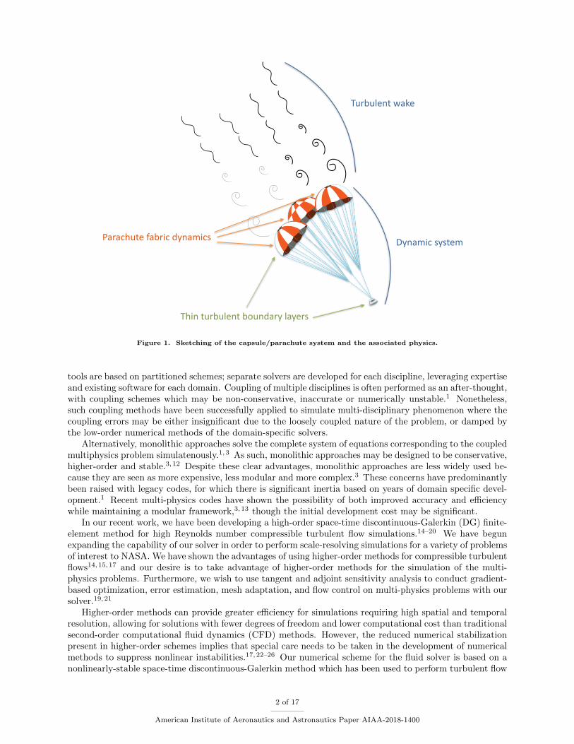
Many engineering systems are inherently multi-disciplinary. Accurate modeling of such systems re-quires the coupling of multiple physical models, with potentially different levels of fidelity and different timescales. Examples include fluid-structure interaction (FSI), aero-thermal heating/conjugate heat transfer,chemically reacting flows, etc.1 In this work, the main target applications is the high-fidelity simulationof capsule/parachute systems for atmospheric entry.2 As shown on Figure 1, this application presents asignificant modeling challenge due to the following features:

• high-Reynolds number flow about the capsule and the parachutes;

• high spatial and temporal resolution required for resolving both the parachute geometry and theturbulent flow;

• the interaction of the turbulent wake from the capsule with the thin and light-weight parachute;

• complex dynamics of the parachute fabric, which could also include the effects of porosity;

• dynamic system of multiple moving bodies with collisions and topology changes.

Many different physical phenomena are involved in this system and the physical models for each of thesephenomena need to be tightly coupled in order to obtain a high-fidelity representation of the problem.

With increased complexity and fidelity of domain specific solvers, multi-physics simulation tools havegenerally been built based on modular frameworks.1,3–11 Typically, numerical methods for such multi-physics

∗USRA/NASA Postdoctoral Program Fellow.†Science and Technology Corp.‡NASA ARC. AIAA Member.

1 of 17

American Institute of Aeronautics and Astronautics Paper AIAA-2018-1400

Turbulentwake

Thinturbulentboundarylayers

Parachutefabricdynamics Dynamicsystem

Figure 1. Sketching of the capsule/parachute system and the associated physics.

tools are based on partitioned schemes; separate solvers are developed for each discipline, leveraging expertiseand existing software for each domain. Coupling of multiple disciplines is often performed as an after-thought,with coupling schemes which may be non-conservative, inaccurate or numerically unstable.1 Nonetheless,such coupling methods have been successfully applied to simulate multi-disciplinary phenomenon where thecoupling errors may be either insignificant due to the loosely coupled nature of the problem, or damped bythe low-order numerical methods of the domain-specific solvers.

Alternatively, monolithic approaches solve the complete system of equations corresponding to the coupledmultiphysics problem simulatenously.1,3 As such, monolithic approaches may be designed to be conservative,higher-order and stable.3,12 Despite these clear advantages, monolithic approaches are less widely used be-cause they are seen as more expensive, less modular and more complex.3 These concerns have predominantlybeen raised with legacy codes, for which there is significant inertia based on years of domain specific devel-opment.1 Recent multi-physics codes have shown the possibility of both improved accuracy and efficiencywhile maintaining a modular framework,3,13 though the initial development cost may be significant.

In our recent work, we have been developing a high-order space-time discontinuous-Galerkin (DG) finite-element method for high Reynolds number compressible turbulent flow simulations.14–20 We have begunexpanding the capability of our solver in order to perform scale-resolving simulations for a variety of problemsof interest to NASA. We have shown the advantages of using higher-order methods for compressible turbulentflows14,15,17 and our desire is to take advantage of higher-order methods for the simulation of the multi-physics problems. Furthermore, we wish to use tangent and adjoint sensitivity analysis to conduct gradient-based optimization, error estimation, mesh adaptation, and flow control on multi-physics problems with oursolver.19,21

Higher-order methods can provide greater efficiency for simulations requiring high spatial and temporalresolution, allowing for solutions with fewer degrees of freedom and lower computational cost than traditionalsecond-order computational fluid dynamics (CFD) methods. However, the reduced numerical stabilizationpresent in higher-order schemes implies that special care needs to be taken in the development of numericalmethods to suppress nonlinear instabilities.17,22–26 Our numerical scheme for the fluid solver is based on anonlinearly-stable space-time discontinuous-Galerkin method which has been used to perform turbulent flow

2 of 17


simulations up to 16th-order accuracy in space and time.17 A space-time finite-element formulation can benaturally extended to moving-domain problems while guaranteeing satisfaction of the geometric conservationlaw (provided sufficient integration is used).27 This has made the space-time DG formulation a naturalchoice for moving-domain and FSI simulations.28–30 Due to the low numerical dissipation present in higher-order schemes, inconsistent coupling of the fluid and structure modules can lead to numerical instabilitiesand catastrophic failures of the simulation.12,28,31 For this reason, a monolithic fully coupled space-timeapproach has been preferred to a partitioned method. This approach ensures discrete conservation, numericalstability and high-order accuracy on the coupled multi-physics problem.12,28

In this work, we discuss the extension of our existing fluid solver to a modular monolithic higher-orderfinite-element based multi-physics solver. We describe some of the challenges and strategies employed. InSection II we describe our existing software framework designed to handle a single physical model. Examplesof some of the physical models and their discretizations are given in Section III. In Section IV we presentthe chosen coupling strategy. Some preliminary numerical results are presented in Section V. Finally, wediscuss future perspectives in Section VI.

II. Single physics module

The existing higher-order space-time discontinuous-Galerkin compressible Navier-Stokes solver is thestarting point of this work.14,15,17 This solver is based on an efficient tensor-product finite-element for-mulation, a Jacobian-free Newton-Krylov solver and tensor-product preconditioners.14,16 The solver hasbeen validated up to 16th-order accuracy on simple test problems15,17 and has been used for performingscale-resolving simulations on a variety of separated flows.15,32

The framework has been extended to allow for several finite-element discretizations (continuous-Galerkin/discontinuous-Galerkin/C1-discontinuous-Galerkin) to be used in combination with different sets of physicsmodules (compressible Navier-Stokes, elasticity, advection-diffusion, etc.). Examples of several physics mod-ules are described in more detail in Section III. An object-oriented methodology is used, whereby mainobjects are responsible for

• defining the mesh and associated fields on the region;

• the finite-element discretization (CG/DG/C1-DG);

• the non-linear and linear solvers;

• handling the primal, tangent and adjoint systems;

• the definition of the physics modules.

In particular, the finite-element discretization of each physical model involves evaluating integrals over theelements and faces of the mesh for computing residuals, linearized residuals, diagnostics etc. Each physicsmodule implements an Application Programming Interface (API) for evaluating the integrands (fluxes, forces,outputs, etc.). The discretization modules implement the computation of the actual integrals by loopingover appropriate elements and faces in the mesh, calling the mesh API to extract data at quadrature pointsand, in turn, calling the physics module APIs to evaluate the appropriate integrands. This modular andobject-oriented implementation allows use of the same objects in different contexts (different physics ordiscretizations, primal or adjoint solve, etc.). The goal is that researchers can focus on their physics/modelimplementation without having to understand the back-end of the solver.

The modular implementation is further complicated by the requirement to support the ability to solvetangent and adjoint problems for sensitivity analysis.19,21 The tangent and adjoint problems are linear sys-tems of equations corresponding to a linearized physical model and its discrete transpose. In this approach,each physics module implements three versions of the integrands (fluxes, outputs functions, etc.) correspond-ing to primal, tangent and adjoint formulations. A common solver is used to converge primal, adjoint andtangent systems, with significant reuse of the discretization related modules. In particular, most operationsin the residual evaluation are symmetric (i.e. apply basis functions - compute integrand - apply transpose ofbasis functions) such that the adjoint can be computed by simply transposing the primal integrand. Specialcare must be taken for certain non-symmetric operations.

The desire to compute the tangent and adjoint for simulations requires significant reading and writingof solution files to disk, as the primal solution for every time-slab must be saved in order to be able to

3 of 17


I/O Solver Diagnostics

Primal

Tangent

Adjoint

Un

V n

Rn(Un) +Gn(Un−1) = 0

∂Rn

∂UnVn + ∂Gn

∂Un−1Vn−1 = −δRn

∂Rn

∂Un

TΨn + ∂Gn

∂Un+1

TΨn+1 = −δJn Ψn

J |n = J(Un)

dJds|n = ∂Jn

∂UnVn + ∂Jn

∂s

δJn

Un

dJds|adjn = ∂Rn

∂s

TΦn

V n−1

V n

Un−1

Un

Ψn+1

ΨndJds =

∑Nn=1

dJds |adjn + 1

N∆t∂Jn

∂s

dJds

= 1N∆t

∑Nn=1

dJds|n

J = 1N∆t

∑Nn=1 J |n

READ

WRITE Un

U 0

READ

WRITE V n

V 0, Un

Un

U 0

V n

δJn = 1N∆t

∂Jn

∂Un

T

δRn δRn = ∂Rn

∂s

UnREAD

WRITE Ψn

Ψ0, Un

Ψn

Figure 2. Flow charts for the primal, tangent, and adjoint solver. The primal solves the governing equations Rn(Un) +

Gn(Un−1) = 0 for a primal solution Un, where Rn and Gn are the residual and temporal source operators, respectively.19

The primal diagnostics module computes an output quantity J |n and its temporal mean J . The tangent and adjointsolvers compute the tangent and adjoint solutions V n and Ψn, respectively. The tangent and adjoint diagnostics modulescompute the sensitivity of the temporal mean J to some input parameter(s) s.

linearize about this solution for the tangent and adjoint solves. Reading and writing to disk can be asignificant bottleneck limiting the performance of the simulation tool. Additionally, parallel input/output(I/O) is known to scale poorly with the number of processors so it can be problematic for massively parallelsimulations. In order to overcome these bottlenecks, asynchronous I/O is performed on a separate setof dedicated cores. A similar approach is used for the computation of diagnostics (cut-planes, integrals,averaging, etc.) which are also computed on a separate set of cores. Figure 2 depicts the process flowbetween I/O, solver, and diagnostics cores for the primal, tangent and adjoint solver.

I/O Solver DiagnosticsTime Step

R1(U1) +G1(U0) = 0

J |1 = J(U1)

U 1

READ

WRITE U 1

U 0U 0

n = 1

n = 2

n = 3 WRITE U 2 J |2 = J(U2)

R2(U2) +G2(U1) = 0

R3(U3) +G3(U2) = 0

U 2

U 3

J = 1N∆t

∑Nn=1 J |n

Figure 3. Flow chart for the primal solver for the first three time steps of a run. The notation is the same as that usedin Figure 2.

There are two main advantages to using dedicated cores for I/O and diagnostics. Firstly, it provides theflexibility to carry out time-consuming tasks like reading and writing a time-slab to disk while computingthe solution at the next time step. Figure 3 illustrates overlapping I/O, the solver and diagnostics forthe primal solver. A similar scheme is used for the tangent and adjoint solvers. By overlapping I/O andcomputation, the tangent and adjoint solvers can compute a time-slab faster than the primal solver.33 The

4 of 17


second advantage of using asynchronous I/O and diagnostics is that the number of cores set aside for I/Ocan be made fairly small to avoid running into scaling issues with parallel I/O.

III. Example Physical Models

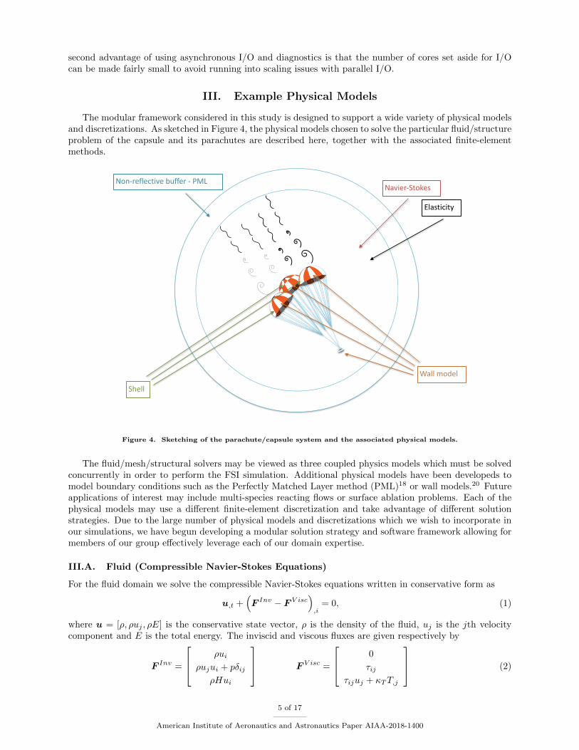
The modular framework considered in this study is designed to support a wide variety of physical modelsand discretizations. As sketched in Figure 4, the physical models chosen to solve the particular fluid/structureproblem of the capsule and its parachutes are described here, together with the associated finite-elementmethods.

Non-reflectivebuffer-PMLNavier-Stokes

Elasticity

Shell

Wallmodel

Figure 4. Sketching of the parachute/capsule system and the associated physical models.

The fluid/mesh/structural solvers may be viewed as three coupled physics models which must be solvedconcurrently in order to perform the FSI simulation. Additional physical models have been developeds tomodel boundary conditions such as the Perfectly Matched Layer method (PML)18 or wall models.20 Futureapplications of interest may include multi-species reacting flows or surface ablation problems. Each of thephysical models may use a different finite-element discretization and take advantage of different solutionstrategies. Due to the large number of physical models and discretizations which we wish to incorporate inour simulations, we have begun developing a modular solution strategy and software framework allowing formembers of our group effectively leverage each of our domain expertise.

III.A. Fluid (Compressible Navier-Stokes Equations)

For the fluid domain we solve the compressible Navier-Stokes equations written in conservative form as

u,t +(F Inv − F V isc

),i

= 0, (1)

where u = [ρ, ρuj , ρE] is the conservative state vector, ρ is the density of the fluid, uj is the jth velocitycomponent and E is the total energy. The inviscid and viscous fluxes are given respectively by

F Inv =

ρui

ρujui + pδij

ρHui

F V isc =

0

τij

τijuj + κTT,j

(2)

5 of 17


where p is the static pressure, δij is the Kronecker delta, H is the total enthalpy, τij is the viscous stresstensor, T is the temperature and κT is the thermal conductivity. The system is closed using the followingrelationships

T =p

ρR, p = (γ − 1)

(ρE − 1

2ρukuk

), τij = µ(ui,j + uj,i)− λuk,kδij , (3)

where R is the gas constant, γ is the specific heat ratio, µ is the dynamic viscosity and λ = 23µ is the bulk

viscosity.We use a space-time discontinuous-Galerkin discretization of (1). We seek a solution u which satisfies

the weak form

∑

κ

∫

I

∫

κ

−(w,tu + w,i(f

Ii − fVi )

)+

∫

I

∫

∂κ

w(f Iini − fVi ni) +

∫

κ

w(tn+1− )u(tn+1

− )−w(tn+)u(tn−)

= 0 (4)

where the second and third integrals arise due to the spatial and temporal discontinuity, respectively, of the

basis functions. f Iini and fVi ni denote single valued numerical flux functions approximating, respectively,the inviscid and viscous fluxes at the spatial boundaries of the elements.

III.B. Elasticity

We solve the equations of linear elasticity to obtain the volume displacement of the fluid mesh given theprescribed motion of the surface (or part of the surface) of the fluid mesh. The equations of linear elasticityare

σij,j = 0 (5)

where σij is the Cauchy stress tensor given by

σij = 2µeεij + λeεkk (6)

µe = E2(1+ν) and λe = µe

2ν1−2ν are the Lame constants given as a function of the Young’s Modulus, E, and

Poisson ratio, ν. The strain tensor, ε is given by

εij = 12 (ui,j + uj,i) (7)

where u is the displacement field. A compact representation of the stress tensor may be given by σij =

Cijklui,j , where Cijkl is the stiffness tensor. We note that we could include an acceleration term in (5) andsolve the equations of linear elasticity as a structural model, though we have yet to apply it for this purpose.When applying the linear elasticity model for mesh deformation, the parameters E and ν may be variedspatially to improve mesh quality. A common choice, employed here, is to fix ν and vary E on each elementproportionally with the inverse of the Jacobian of mapping from reference to physical space.34

We apply a continuous finite-element discretization of (5) over the initial mesh of the fluid domain. Defin-ing V =

w ∈ H1(Ω× I),w|κ ∈ [P(κ× I)]3

, the space-time finite-element space consists of C0 continuous

piece-wise polynomial functions on each element.We seek solutions u ∈ VE satisfying

∑

κ

−∫I

∫

κ0

wi,jCijkluk,l +

∫

I

∫

∂κ0∩∂Ω

wiCijkluk,lnj

= 0. (8)

We note that the integration is performed over the initial spatial mesh (i.e elements κ0) of the fluid domainextruded in time, as opposed to the deformed mesh. An alternative approach is to integrate over the initialspatial mesh for each time-slab, which may potentially allow for larger mesh deformations. However, thislater approach results in a scheme where the mesh deformation is a function of not only the given boundarydisplacement but the entire displacement history. More details about the linear elasticity solver can be foundin Diosady and Murman.35

6 of 17


III.C. Shell

The fabric of parachutes is modeled using the linear shell equations, which are the same as the linearelasticity equations; however, under the assumption of simplified shell kinematics one needs to solve only forthe displacement of the mid-plane of the shell. This reduces the dimensionality of the problem by one. Theweak form of the shell equations are given by:

∑

κ

∫

I

∫

κ0

(−wi,tyi,t +Hαβ(w)

Eh

1− ν2CαβγθHγθ(y) +Bαβ(w)

Eh3

1− ν2CαβγθBγθ(y) + wiτijyj

)= 0 (9)

The terms for the above equation are defined in detail in Burgess et al.36

As with the elasticity model, we integrate over the initial (reference) surface in the spatial direction. Thefirst term corresponds to an acceleration term, the second and third terms correspond to internal energiesdue to in-plane and bending strains respectively, while the final term corresponds to work done by externalforcing (i.e. forcing due to surface tractions τij from the fluid). The in-plane and bending strain terms arefunctions of the displacement y, (see Burgess et al.36 for full details). We note that we directly discretizethe structural velocity y,t using a basis which is piece-wise discontinuous in time and piece-wise continuousin space. The displacement y which is C0 continuous in both space and time, is given by directly integratingy,t.

III.D. Perfectly Matched Layer Method

In order to limit spurious acoustic reflections from boundaries of the fluid domain we use a Perfectly MatchedLayer (PML) technique on far field boundaries. The PML technique involves solving the compressible Navier-Stokes equations with a forcing term and a set of auxiliary equations corresponding to each conservationlaw in a buffer region near the boundary of the fluid domain. Details of the PML technique are given inGarai et al.18 In this multi-physics context, the PML technique may be viewed as solving a different physicalmodel in the buffer region coupled to the fluid region through a Riemann solver at the interface of the fluidand buffer regions. The PML region is discretized using a space-time discontinuous-Galerkin finite-elementmethod in the same manner as the fluid region. For simplicity, we assume a fixed spatial mesh in the PMLregion.

III.E. Wall Model

Due to the large range in scales present in turbulent flows, the resolution required to fully resolve the near-wallregion makes Direct Numerical Simulation (DNS) and Large Eddy Simulation (LES) prohibitively expensivefor high-Reynolds number wall-bounded flows. Modeling the near-wall region is necessary in order to makeindustrial computations practical. In Carton de Wiart and Murman,20 the coupling of the space-time DGsolver with several simple wall modeling approaches have been studied. In these modeling approaches, theinner part of the boundary layer is not computed but information from the fluid away from the wall is usedto evaluate a modified boundary condition which is then applied at the wall. In the simplest cases the wallmodel may consist of analytic equations, for example based on the logarithmic law. More complex models,for instance, based on thin boundary layer approximations or integral wall models, can be used to increasethe accuracy of the wall model. We therefore treat the wall model as a separate physics module, instead of asimple boundary condition. By defining simple input/output to the fluid domain, we are able to experimentwith different modeling approaches without making any major modifications to the fluids module. The wallmodel is discretized using an appropriate finite-element method on a surface mesh of the fluid domain.

IV. A Multi-Physics Monolithic Solver

In this section, the strategy to transform the “single-physics” solver into a multi-physics monolithic solveris described. The capsule/parachute system and the accompanying physical model presented in Figure 4 isused here to illustrate the coupling procedure and the associated challenges.

The multi-physics domain is split into “regions”, each corresponding to the discretization of a singlephysics model on a given computational mesh. Each region is responsible for computing local residual termsand auxiliary data, which could be sent to other regions. For the capsule/parachute system described inFigure 4, the elasticity and Navier-Stokes physics are defined as separate regions, although they are defined

7 of 17


on the same mesh partition. The same goes for the shell and the wall model modules on the parachutes.They are also defined as separated regions, even though they are defined on the same boundary mesh.Splitting the global problem based on physics/mesh/discretization allows the solver to load balance eachregion independently. It also gives a lot of flexibility as new physics or discretizations can be added into thesolver without impacting the other modules.

We can define the global problem as multiple regions, linked together through coupling operations. Asstated in Section II, each region can also be split into three sub-regions, each responsible for specific work:solver, I/O and diagnostics. This is handled in the framework by defining groups of cores, where groupis associated with one region and one set of operations (solver, I/O or diagnostics), creating a matrix ofcommunicators, linked together by intra- and inter-communicators. Inter-communicators are used by thecoupling objects to communicate data from one region to another. They are also used within a region tosend the solution from the solver nodes to the I/O or diagnostics nodes, or the other way around. Intra-communicators encompass a group of (sub-)regions and are used mostly to synchronize the regions together,for instance by broadcasting the value of the time when restarting a simulation by reading an initial solutionor gathering the residual norm at the non-linear/linear solver levels. Figure 5 illustrates the matrix ofcommunicators in the context of the capsule/parachute system. Communicators are only created between

Figure 5. Matrix of communicators between the different sub-regions. Local communicators and denoted by graysquares, intra-communicators by red grouping and inter-communicators by blue arrows.

rows and columns, not diagonally. As regions can also be locally partitioned, local communicators are usedto communicate the solution between the different region partitions.

Even though the global problem is split into several regions, it is still tightly coupled by communicatingthe appropriate data between the different regions (i.e. boundary state, boundary stress, displacement, etc.).These coupling data are then used inside boundary conditions or domain forcing functions. As stated inSection II, the framework uses a space-time finite-element method, which requires the solution of a non-linearsystem at each time step using a Newton-Krylov approach. This gives three main loops in the system: atemporal loop, a non-linear solver loop and a linear solver loop. The different loops are presented in Figure 6,showing where the coupling needs to occur. The coupling between the different regions will occur at everylevel of the code, from the temporal loop all the way down to the linear solver. In the temporal loop, couplingmay occur after solving the non-linear system in order to compute diagnostics that can depend on couplingdata (cut planes, average, boundary integrals, etc.). The coupling also occurs at every non-linear and linearsolver iteration. Indeed, in a monolithic approach, the state u and residual R vectors are formed over alldegrees of freedom corresponding to the coupled equations, therefore spanning all the different regions (i.e.fluid/mesh/structure/PML/wall-model)

u =

u1

u2

...

un

R =

R1

R2

...

Rn

. (10)

The residual vector can be split into multiple residual vectors Ri, each vector associated with one region

Ri = Ri(ui,αi1,αi2, . . . ,αij), (11)

8 of 17


Temporalloop

Updateubysolvingnon-linearsystemR(u)

Computingquantityofinterest(integrals,mean,etc.)

Computecouplingαik

Non-linearsolverloop

Computenon-linearresidualR(u)

SolvelinearsystemΔu=-(dR/du)-1R(u)

Computecouplingαik

Linearsolverloop

ComputelinearizedresidualRlin(v)

Computecouplingαlinik

Figure 6. Temporal (black), non-linear solver (red) and linear solver (green) loops with associated operations.

where ui the local vector state and αij = αij(uj ,αjk) represents the vector of coupling data shared betweenregions i and j (which can also depend on the coupling data αjk between region j and another region k).At each time-slab, the non-linear system

R(u) = 0 (12)

must be solved globally. The same Jacobian-free Newton-Krylov scheme previously developed for the fluidmodule14 is used to drive the residual towards zero. The Newton-Krylov solver involves the repeated eval-uation of residuals and linearized residuals at each Newton and Krylov iteration, respectively. The Newtonsolver updates the state at each iteration using

uk+1 = uk + ∆uk with ∆uk = −(∂R

∂u

)−1

R(uk), (13)

where k is the Newton iteration number. This linear system is then solved using a Krylov method inwhich linearized residual vectors Rlin

i (ui,αij ;ulini ,αlinij ) are evaluated, where ui and αlinij are the linearized

state and linearized coupling data, respectively. The evaluation of the linearized residual involves similarinteractions between modules.

1

RWM(UWM,…) RPML(UPML,…) RShell(UShell,…)RNS(UNS,…) REL(UEL,…)

RPMLRWM RNS RShell REL

!wall(UWM,…)Ub(UPML) 'X(UEL)

'Xb(UShell)

UPMLUWMUNS UShell UEL

!b(UNS,'X,!wall)Ub(UNS,'X)

UI(UNS,'X)

Figure 7. Coupling of physics modules for primal residual evaluation. U denotes the state vector, while R denotes theresidual vector. Each box depict a physics module; WM: wall model, PML: perfectly matched layer buffer region, NS:Navier-Stokes equations for fluid region, Shell: linear shell model, EL: linear-elastic mesh deformation. The quantitiestransferred between different physics modules are wall stress, τw, boundary state Ub, extracted state for fluid volumeUe, boundary displacement Xw, mesh coordinates X.

9 of 17


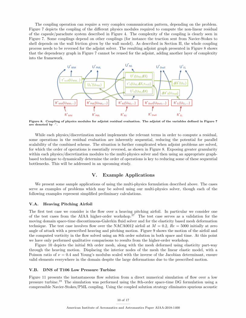
The coupling operation can require a very complex communication pattern, depending on the problem.Figure 7 depicts the coupling of the different physics modules required to compute the non-linear residualof the capsule/parachute system described in Figure 4. The complexity of the coupling is clearly seen inFigure 7. Some couplings depend on other couplings (for instance the traction sent from Navier-Stokes toshell depends on the wall friction given by the wall model). As described in Section II, the whole couplingprocess needs to be reversed for the adjoint solver. The resulting adjoint graph presented in Figure 8 showsthat the dependency graph in Figure 7 cannot be reused for the adjoint, adding another layer of complexityinto the framework.

2

R*WM(UWM,…) R*PML(UPML,…) R*Shell(UShell,…)R*NS(UNS,…) R*EL(UEL,…)

R*PMLR*WM R*NS R*Shell R*EL

!*wall(UWM,…)Ub*(UPML) 'X*(UEL)

'X*b(UShell)

U*PMLU*WMU*NS U*Shell U*EL

!*b(UNS,'X,!wall)U*b(UNS,'X)

U*I(UNS,'X)

Figure 8. Coupling of physics modules for adjoint residual evaluation. The adjoint of the variables defined in Figure 7are denoted by ·∗.

While each physics/discretization model implements the relevant terms in order to compute a residual,some operations in the residual evaluation are inherently sequential, reducing the potential for parallelscalability of the combined scheme. The situation is further complicated when adjoint problems are solved,for which the order of operations is essentially reversed, as shown in Figure 8. Exposing greater granularitywithin each physics/discretization modules to the multi-physics solver and then using an appropriate graph-based technique to dynamically determine the order of operations is key to reducing some of these sequentialbottlenecks. This will be addressed in an upcoming study.

V. Example Applications

We present some sample applications of using the multi-physics formulation described above. The casesserve as examples of problems which may be solved using our multi-physics solver, though each of thefollowing examples represent simplified preliminary calculations.

V.A. Heaving Pitching Airfoil

The first test case we consider is the flow over a heaving pitching airfoil. In particular we consider oneof the test cases from the AIAA higher-order workshop.37 The test case serves as a validation for themoving domain space-time discontinuous-Galerkin fluid solver and for the elasticity based mesh deformationtechnique. The test case involves flow over the NACA0012 airfoil at M = 0.2, Re = 5000 initially at zeroangle of attack with a prescribed heaving and pitching motion. Figure 9 shows the motion of the airfoil andthe computed vorticity in the flow solved using an 8th order solution in both space and time. At this pointwe have only performed qualitative comparisons to results from the higher-order workshop.

Figure 10 depicts the initial 8th order mesh, along with the mesh deformed using elasticity part-waythrough the heaving motion. Displacing the interior nodes of the mesh the linear elastic model, with aPoisson ratio of ν = 0.4 and Young’s modulus scaled with the inverse of the Jacobian determinant, ensurevalid elements everywhere in the domain despite the large deformations due to the prescribed motion.

V.B. DNS of T106 Low Pressure Turbine

Figure 11 presents the instantaneous flow solution from a direct numerical simulation of flow over a lowpressure turbine.18 The simulation was performed using the 8th-order space-time DG formulation using acompressible Navier-Stokes/PML coupling. Using the coupled solution strategy eliminates spurious acoustic

10 of 17


Figure 9. Vorticity magnitude for Heaving/Pitching NACA0012 airfoil.

11 of 17


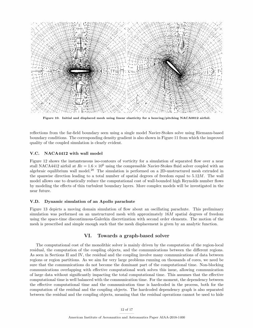
Figure 10. Initial and displaced mesh using linear elasticity for a heaving/pitching NACA0012 airfoil.

reflections from the far-field boundary seen using a single model Navier-Stokes solve using Riemann-basedboundary conditions. The corresponding density gradient is also shown in Figure 11 from which the improvedquality of the coupled simulation is clearly evident.

V.C. NACA4412 with wall model

Figure 12 shows the instanteneous iso-contours of vorticity for a simulation of separated flow over a nearstall NACA4412 airfoil at Re = 1.6× 106 using the compressible Navier-Stokes fluid solver coupled with analgebraic equilibrium wall model.20 The simulation is performed on a 2D-unstructured mesh extruded inthe spanwise direction leading to a total number of spatial degrees of freedom equal to 5.12M . The wallmodel allows one to drastically reduce the computational cost of wall-bounded high Reynolds number flowsby modeling the effects of thin turbulent boundary layers. More complex models will be investigated in thenear future.

V.D. Dynamic simulation of an Apollo parachute

Figure 13 depicts a moving domain simulation of flow about an oscillating parachute. This preliminarysimulation was performed on an unstructured mesh with approximately 16M spatial degrees of freedomusing the space-time discontinuous-Galerkin discretization with second order elements. The motion of themesh is prescribed and simple enough such that the mesh displacement is given by an analytic function.

VI. Towards a graph-based solver

The computational cost of the monolithic solver is mainly driven by the computation of the region-localresidual, the computation of the coupling objects, and the communications between the different regions.As seen in Sections II and IV, the residual and the coupling involve many communications of data betweenregions or region partitions. As we aim for very large problems running on thousands of cores, we need besure that the communications do not become the dominant part of the computational time. Non-blockingcommunications overlapping with effective computational work solves this issue, allowing communicationof large data without significantly impacting the total computational time. This assumes that the effectivecomputational time is well balanced with the communication time. For the moment, the dependency betweenthe effective computational time and the communication time is hardcoded in the process, both for thecomputation of the residual and the coupling objects. The hardcoded dependency graph is also separatedbetween the residual and the coupling objects, meaning that the residual operations cannot be used to hide

12 of 17


(a) Isosurfaces of Vorticity.

(b) Density Gradient using Riemann BC.

(c) Density Gradient using PML.

Figure 11. Direct numerical simulation of a T106 low pressure turbine with and without PML.18

13 of 17


Figure 12. NACA4412 at near-stall conditions with instantaneous iso-contours of vorticity colored by velocity magni-tude.20

Figure 13. Mach number contours of a dynamic simulation of an Apollo parachute.

14 of 17


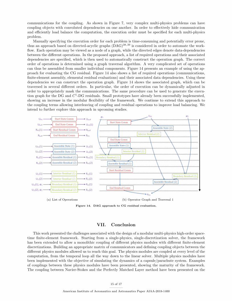
communications for the coupling. As shown in Figure 7, very complex multi-physics problems can havecoupling objects with convoluted dependencies on one another. In order to effectively hide communicationand efficiently load balance the computation, the execution order must be specified for each multi-physicsproblem.

Manually specifying the execution order for each problem is time-consuming and potentially error prone,thus an approach based on directed-acyclic graphs (DAG)38,39 is considered in order to automate the work-flow. Each operation may be viewed as a node of a graph, while the directed edges denote data-dependenciesbetween the different operations. In the proposed approach, a list of required operations and their associateddependencies are specified, which is then used to automatically construct the operation graph. The correctorder of operations is determined using a graph traversal algorithm. A very complicated set of operationscan thus be assembled from smaller individual components. Figure 14 presents an example of using the ap-proach for evaluating the CG residual. Figure 14 also shows a list of required operations (communications,finite-element assembly, elemental residual evaluations) and their associated data dependencies. Using thesedependencies we can construct the operation graph. Figure 14 shows the associated graph, which can betraversed in several different orders. In particular, the order of execution can be dynamically adjusted inorder to appropriately mask the communications. The same procedure can be used to generate the execu-tion graph for the DG and C1-DG residuals. Small prototypes have already been successfully implemented,showing an increase in the modular flexibility of the framework. We continue to extend this approach tothe coupling terms allowing interleaving of coupling and residual operations to improve load balancing. Weintend to further explore this approach in upcoming studies.

10

Assemble State (1)

Interior Residual (1)

Boundary Residual (1)

Start State Comm

End Residual Comm

Assemble Residual (1)

End State Comm

Start Residual Comm

Assemble State (2)



Assemble Residual (2) RH1(2)RL2(2)

RH1(1)RL2(1)

UH1(1)

UH1(2)

UL2(1)

UL2(2)

UL2(1)

UL2(2)

UL2(1),D1

UL2(2),D2

RL2(1)

RL2(2)

RL2(1)

RL2(2)

RH1(1) Rbuff

Rbuff RH1

UH1

UH1(1)

Ubuff

Ubuff

(a) List of Operations

Assemble State (1)



Start State Comm

End Residual Comm


End State Comm

Start Residual Comm

Assemble State (2)




D1 D2UH1

RH1

(b) Operator Graph and Traversal 1

Figure 14. DAG approach to CG residual evaluation.

VII. Conclusion

This work presented the challenges associated with the design of a modular multi-physics high-order space-time finite-element framework. Starting from a single-physics, single-discretization solver, the frameworkhas been extended to allow a monolithic coupling of different physics modules with different finite-elementdiscretizations. Building an appropriate matrix of communicators and defining coupling objects between thedifferent physics modules allowed us to reach this goal. The physics modules are coupled at every level of thecomputation, from the temporal loop all the way down to the linear solver. Multiple physics modules havebeen implemented with the objective of simulating the dynamics of a capsule/parachute system. Examplesof couplings between these physics modules have been presented, showing the maturity of the framework.The coupling between Navier-Stokes and the Perfectly Matched Layer method have been presented on the

15 of 17


challenging scale-resolving simulation of a low pressure turbine blade, showing the advantages of the non-reflective approach for the domain inflow and outflow. The ability of the solver to deform a mesh usingthe linear elasticity equation and exchange the updated mesh with Navier-Stokes has been shown for aheaving/pitching airfoil. Wall modeling has also been tested in order to decrease the cost of running wall-bounded high-Reynolds number flows. Treating the wall model as a separate physics enables better loadbalancing of the problem and greater flexibility as the different models can be easily tested in the sameframework. Finally, preliminary computation of a single parachute with no capsule have been performed,paving the way to a fully coupled simulation of the capsule/parachute system.

Many improvements can be made to the framework. The efficieny and robustness of the non-linear solverneeds to be further improved and more advanced preconditioning techniques need be implemented. Theimpact of coupling multiple physics on the non-linear system need to be further analyzed and the differentphysics modules need to be tuned in order to obtain a better conditioned system. For the moment, theload balancing of the global multi-physics system is done by the user. A more automated approach willbe considered, where the software will automatically distribute the cores between the different regions asa function of the size of the problem and the cost of each physics/discretization. Finally, a graph-basedapproach will be considered in order to remove the need of hard-coding the dependency graph betweenthe different coupling/residual operators. This will allow a better load balancing of the operations whilstimproving the global modularity of the framework.

References

1Keyes, D., McInnes, L. C., and CarolWoodward, “Multiphysics Simulations: Challenges and Opportunities,” ArgonneNational Laboratory ANL/MCS-TM-321, 2011.

2Ray, E. S., “Test Vehicle Forebody Wake Effects on CPAS Parachutes,” AIAA Paper AIAA-xxxx, 2017.3Heil, M., Hazel, A. L., and Boyle, J., “Solvers for large-displacement fluid–structure interaction problems: segregated

versus monolithic approaches,” Computational Mechanics, Vol. 43, 2008, pp. 91–101.4McDaniel, D. R., Tuckey, T., and Morton., S. A., “The HPCMP CREATETM-AV Kestrel Computational Environment

and its Relation to NASA’s CFD Vision 2030,” AIAA 2017-0813, 2017.5McDaniel, D. R. and Tuckey, T., “Multiple Bodies, Motion, and Mash-Ups: Handling Complex Use-Cases with Kestrel,”

AIAA 2014-0415, 2014.6Jayaraman, B., Wissink, A., Shende, S., Adamec, S., and Sankaran, V., “Extensible Software Engineering Practices for

the Helios High-Fidelity Rotary-Wing Simulation Code,” AIAA 2011-1178, 2011.7Wissink, A. M., Sitaraman, J., Sankaran, V., Mavriplis, D. J., and Pulliam, T. H., “A Multi-Code Python-Based

Infrastucture for Overset CFD with Adaptive Cartesian Grids,” AIAA 2008-0927, 2008.8Atwood, C. A., Adamec, S. A., Murphy, M. D., Post, D. E., and Blair, L., “Collaborative software development of scalable

DoD computational engieering,” DoD HPCMP User Group Conference, 2010.9Kiris, C. C., Barad, M. F., Housman, J. A., Sozer, E., Brehm, C., and Moini-Yekta, S., “The LAVA Computational Fluid

Dynamics Solver,” AIAA 2014-0070, 2014.10Gaston, D., Newman, C., Hansen, G., and Lebrun-Grandie, D., “MOOSE: A parallel computational framework for

coupled systems of nonlinear equations,” Nuclear Engineering and Design, Vol. 239, 2009, pp. 1768–1778.11Farhat, C., van der Zee, G., and Geuzaine, P., “Provably second-order time-accurate loosely-coupled solution algorithms

for transient nonlinear compuational aeroelasticity,” CMAME , Vol. 195, 2006, pp. 1973–2001.12van Brummelen, E., Hulshoff, S., and de Borst, R., “A monolithic approach to fluid-structure interaction using space-time

finite elements,” Comput. Methods Appl. Mech. Engrg., Vol. 2003, 2003, pp. 2727–2748.13Kenway, G. K. W., Kennedy, G. J., and Martins, J. R. R. A., “Scalable Parallel Approach for High-Fidelity Steady-State

Aeroelastic Analysis and Adjoint Derivative Computations,” AIAA Journal , Vol. 52, 2014, pp. 935–951.14Diosady, L. T. and Murman, S. M., “Design of a variational multiscale method for turbulent compressible flows,” AIAA

Paper 2013-2870, 2013.15Diosady, L. T. and Murman, S. M., “DNS of flows over periodic hills using a discontinuous Galerkin spectral element

method,” AIAA Paper 2014-2784, 2014.16Diosady, L. T. and Murman, S. M., “Tensor-Product Preconditioners for Higher-order Space-Time Discontinuous Galerkin

Methods,” Journal of Computational Physics, Vol. 330, 2017, pp. 296–318.17Diosady, L. T. and Murman, S. M., “Higher-Order Methods for Compressible Turbulent Flows Using Entropy Variables,”

AIAA Paper 2015-0294, 2015.18Garai, A., Diosady, L., Murman, S., and Madavan, N., “Development of a Perfectly Matched Layer Technique for a

Discontinuous-Galerkin Spectral-Element Method,” AIAA 2016-1338, 2016.19Ceze, M., Diosady, L. T., and Murman, S. M., “Development of a High-Order Space-Time Matrix-Free Adjoint Solver,”

AIAA Paper 2016-0833, 2016.20Carton de Wiart, C. and Murman, S. M., “Assessment of Wall-modeled LES Strategies Within a Discontinuous-Galerkin

Spectral-element Framework,” AIAA 2017-1223, 2017.21Blonigan, P., Fernandez, P., Murman, S., Wang, Q., G., R., and Magri, L., “Toward a chaotic adjoint for LES,” Center

for Turbulence Research Proceedings of the Summer Program 2016 , 2016.

16 of 17


22Orszag, S. and Patterson, G.S., J., “Numerical simulation of turbulence,” Statistical Models and Turbulence, edited byM. Rosenblatt and C. Atta, Vol. 12 of Lecture Notes in Physics, Springer Berlin Heidelberg, 1972, pp. 127–147.

23Morinishi, Y., Lund, T. S., Vasilyev, O. V., and Moin, P., “Fully Conservative Higher Order Finite Difference Schemesfor Incompressible Flow,” Journal of Computational Physics, Vol. 143, 1998, pp. 90–124.

24Honein, A. E. and Moin, P., “Higher entropy conservation and numerical stability of compressible turbulence simulations,”Journal of Computational Physics, Vol. 201, 2004, pp. 531–545.

25Subbareddy, P. K. and Candler, G. V., “A fully discrete, kinetic energy consistent finite-volume scheme for compressibleflows,” Journal of Computational Physics, Vol. 228, No. 5, 2009, pp. 1347 – 1364.

26Sjogreen, B. and Yee, H., “On Skew-Symmetric Splitting and Entropy Conservation Schemes for the Euler Equations,”Numerical Mathematics and Advanced Applications 2009 , edited by G. Kreiss, P. Lotstedt, A. Malqvist, and M. Neytcheva,Springer Berlin Heidelberg, 2010, pp. 817–827.

27Lesoinne, M. and Farhat, C., “Geometric conservation laws for flow problems with moving boundaries and deformablemeshes, and their impact on aeroelastic computations,” Comput. Methods Appl. Mech. Engrg., Vol. 134, 1996, pp. 71–90.

28Hubner, B., Walhorn, E., and Dinkler, D., “A monolithic approach to fluid-structure interaction using space-time finiteelements,” Comput. Methods Appl. Mech. Engrg., Vol. 2004, 2004, pp. 2087–2104.

29Tezduyar, T. E. and Sathe, S., “Modelling of fluid-structure interactions with the space-time finite elements: Solutiontechniques,” Int. J. Numer. Meth. Fluids, Vol. 54, 2007, pp. 855–900.

30Wang, L. and Persson, P.-O., “A high-order discontinuous Galerkin method with unstructured space-time meshes fortwo-dimensional compressible flows on domains with large deformations,” Computers and Fluids, Vol. 118, 2015, pp. 53–68.

31Kirby, R. E., Yosibach, Z., and Karniadakis, G. E., “Towards stable coupling methods for high-order discretizations offluid-structure interaction: Algorithms and observations,” Journal of Computational Physics, Vol. 223, 2007, pp. 489–518.

32Garai, A., Diosady, L., Murman, S., and Madavan, N., “Scale-Resolving Simulations of Bypass Transition in a High-Pressure Turbine Cascade Using a Spectral-Element Discontinuous Galerkin Method,” ASME. J. Turbomach, 2017.

33Blonigan, P. J., “Adjoint sensitivity analysis of chaotic dynamical systems with non-intrusive least squares shadowing,”Journal of Computational Physics, Vol. 348, 2017, pp. 803–826.

34K. Stein, T. T. and Benney, R., “Mesh Moving Techniques for Fluid-Structure Interactions With Large Displacements,”J. Appl. Mech, Vol. 70, No. 1, 2003, pp. 58–63.

35Diosady, L. T. and Murman, S. M., “A linear-elasticity solver for higher-order space-time mesh deformation,” AIAASciTech Forum, January 2018, Kissimmee, Florida, 2018.

36Burgess, N., Diosady, L., and Murman, S., “A C1-discontinuous-Galerkin Spectral-element Shell Structural Solver,”AIAA 2017-3727, 2017.

37Wang, Z., Fidkowski, K., Abgrall, R., Bassi, F., Caraeni, D., Cary, A., Deconinck, H., Hartmann, R., Hillewaert, K.,Huynh, H., Kroll, N., May, G., Persson, P.-O., van Leer, B., and Visbal, M., “High-Order CFD Methods: Current Status andPerspective,” International Journal for Numerical Methods in Fluids, Vol. 72, 2013, pp. 811–845.

38Mikida, E., Jain, N., Gonsiorowski, E., Barnes, Jr., P. D., Jefferson, D., Carothers, C. D., and Kale, L. V., “TowardsPDES in a Message-Driven Paradigm: A Preliminary Case Study Using Charm++,” ACM SIGSIM Conference on Principlesof Advanced Discrete Simulation (PADS), SIGSIM PADS ’16 (to appear), ACM, May 2016.

39Berzins, M., Meng, Q., Schmidt, J., and Sutherland, J. C., “DAG-Based Software Frameworks for PDEs,” Proceedings ofthe 2011 International Conference on Parallel Processing, Euro-Par’11, Springer-Verlag, Berlin, Heidelberg, 2012, pp. 324–333.

17 of 17


design of a modular monolithic implicit solver for multi ...€¦ · stability and high-order...

Documents