design of a low-cost underwater acoustic modem for short...
TRANSCRIPT

UNIVERSITY OF CALIFORNIA, SAN DIEGO
Design of a Low-cost Underwater Acoustic Modem for Short-RangeSensor Networks
A thesis submitted in partial satisfaction of the
requirements for the degree
Doctor of Philosophy
in
Computer Science and Engineering
by
Bridget Benson
Committee in charge:
Professor Ryan Kastner, ChairProfessor Rajesh GuptaProfessor John HildebrandProfessor Tajana RosingProfessor Curt Schurgers
2010

Copyright
Bridget Benson, 2010
All rights reserved.

The thesis of Bridget Benson is approved, and it is ac-
ceptable in quality and form for publication on microfilm
and electronically:
Chair
University of California, San Diego
2010
iii

DEDICATION
To everyone who told me not to give up.
iv

EPIGRAPH
Enjoy the Process
—Dr. Dan Clark
v

TABLE OF CONTENTS
Signature Page . . . . . . . . . . . . . . . . . . . . . . . . . . . . . . . . . . iii
Dedication . . . . . . . . . . . . . . . . . . . . . . . . . . . . . . . . . . . . . iv
Epigraph . . . . . . . . . . . . . . . . . . . . . . . . . . . . . . . . . . . . . v
Table of Contents . . . . . . . . . . . . . . . . . . . . . . . . . . . . . . . . . vi
List of Figures . . . . . . . . . . . . . . . . . . . . . . . . . . . . . . . . . . ix
List of Tables . . . . . . . . . . . . . . . . . . . . . . . . . . . . . . . . . . . xii
Acknowledgements . . . . . . . . . . . . . . . . . . . . . . . . . . . . . . . . xiii
Vita and Publications . . . . . . . . . . . . . . . . . . . . . . . . . . . . . . xv
Abstract of the Dissertation . . . . . . . . . . . . . . . . . . . . . . . . . . . xvii
Chapter 1 Introduction . . . . . . . . . . . . . . . . . . . . . . . . . . . . 1
Chapter 2 Motivating Applications . . . . . . . . . . . . . . . . . . . . . 42.1 Coral Reefs . . . . . . . . . . . . . . . . . . . . . . . . . 42.2 Autonomous Drifter Swarms . . . . . . . . . . . . . . . . 72.3 Shallow Water Moorings . . . . . . . . . . . . . . . . . . 82.4 Power Utilities . . . . . . . . . . . . . . . . . . . . . . . . 102.5 Summary . . . . . . . . . . . . . . . . . . . . . . . . . . 11
Chapter 3 Comparison or RF, Optical and Acoustic Communication Un-derwater . . . . . . . . . . . . . . . . . . . . . . . . . . . . . . 123.1 Radio Frequency Waves . . . . . . . . . . . . . . . . . . . 12
3.1.1 Conductivity . . . . . . . . . . . . . . . . . . . . 133.1.2 Wavelength . . . . . . . . . . . . . . . . . . . . . 143.1.3 Air/Water Interface . . . . . . . . . . . . . . . . . 153.1.4 Existing RF Systems . . . . . . . . . . . . . . . . 16
3.2 Optical Waves . . . . . . . . . . . . . . . . . . . . . . . . 183.2.1 Physics of Optical Waves Underwater . . . . . . . 183.2.2 Existing Optical Systems . . . . . . . . . . . . . . 21
3.3 Acoustic Waves . . . . . . . . . . . . . . . . . . . . . . . 223.3.1 Absorption Loss . . . . . . . . . . . . . . . . . . . 223.3.2 Spreading Loss . . . . . . . . . . . . . . . . . . . 243.3.3 Noise . . . . . . . . . . . . . . . . . . . . . . . . . 243.3.4 Passive Sonar Equation . . . . . . . . . . . . . . . 27
vi

3.3.5 Multipath . . . . . . . . . . . . . . . . . . . . . . 293.4 Summary . . . . . . . . . . . . . . . . . . . . . . . . . . 30
Chapter 4 Existing Underwater Acoustic Modems . . . . . . . . . . . . . 324.1 Commercial Modems . . . . . . . . . . . . . . . . . . . . 324.2 Research Modems . . . . . . . . . . . . . . . . . . . . . . 374.3 Summary . . . . . . . . . . . . . . . . . . . . . . . . . . 39
Chapter 5 Transducer Design . . . . . . . . . . . . . . . . . . . . . . . . 425.1 Piezo Ceramics . . . . . . . . . . . . . . . . . . . . . . . 42
5.1.1 Type . . . . . . . . . . . . . . . . . . . . . . . . . 435.1.2 Geometry . . . . . . . . . . . . . . . . . . . . . . 44
5.2 Transducer Construction . . . . . . . . . . . . . . . . . . 465.2.1 Wiring . . . . . . . . . . . . . . . . . . . . . . . . 475.2.2 Potting . . . . . . . . . . . . . . . . . . . . . . . . 475.2.3 Reducing Unwanted Acoustic Radiation . . . . . . 495.2.4 Material Costs . . . . . . . . . . . . . . . . . . . . 50
5.3 Calibration Procedures . . . . . . . . . . . . . . . . . . . 505.3.1 Comparison Method . . . . . . . . . . . . . . . . 505.3.2 Reciprocity Method . . . . . . . . . . . . . . . . . 51
5.4 Experimental Measurements . . . . . . . . . . . . . . . . 535.5 Summary . . . . . . . . . . . . . . . . . . . . . . . . . . 57
Chapter 6 Analog Transceiver Design . . . . . . . . . . . . . . . . . . . . 586.1 Power Amplifier Design . . . . . . . . . . . . . . . . . . . 586.2 Power Management Circuit . . . . . . . . . . . . . . . . . 676.3 Impedance Matching Circuit . . . . . . . . . . . . . . . . 686.4 Pre-Amplifier Design . . . . . . . . . . . . . . . . . . . . 776.5 Summary . . . . . . . . . . . . . . . . . . . . . . . . . . 80
Chapter 7 Digital Design . . . . . . . . . . . . . . . . . . . . . . . . . . . 817.1 Modulation Schemes . . . . . . . . . . . . . . . . . . . . 817.2 Hardware Platforms . . . . . . . . . . . . . . . . . . . . . 857.3 Digital Transceiver . . . . . . . . . . . . . . . . . . . . . 87
7.3.1 Modulator . . . . . . . . . . . . . . . . . . . . . . 897.3.2 Digital Down Converter . . . . . . . . . . . . . . 907.3.3 Symbol Synchronizer . . . . . . . . . . . . . . . . 917.3.4 Demodulator . . . . . . . . . . . . . . . . . . . . 1047.3.5 Clock Generation . . . . . . . . . . . . . . . . . . 1057.3.6 HW/SW Co-Design Controller . . . . . . . . . . . 106
7.4 Resource Requirements . . . . . . . . . . . . . . . . . . . 1087.5 Summary . . . . . . . . . . . . . . . . . . . . . . . . . . 110
vii

Chapter 8 System Tests . . . . . . . . . . . . . . . . . . . . . . . . . . . 1118.1 Analog Testing . . . . . . . . . . . . . . . . . . . . . . . 1118.2 Digital Testing . . . . . . . . . . . . . . . . . . . . . . . . 114
8.2.1 Hard Wired Tests . . . . . . . . . . . . . . . . . . 1148.2.2 Bucket Tests . . . . . . . . . . . . . . . . . . . . . 118
8.3 Integrated Tests . . . . . . . . . . . . . . . . . . . . . . . 1208.3.1 Multipath Measurements . . . . . . . . . . . . . . 1208.3.2 Tank Tests . . . . . . . . . . . . . . . . . . . . . . 1218.3.3 Canyon View Pool Tests . . . . . . . . . . . . . . 1238.3.4 Westlake Tests . . . . . . . . . . . . . . . . . . . 1248.3.5 Integrated System Test Summary . . . . . . . . . 128
8.4 Summary . . . . . . . . . . . . . . . . . . . . . . . . . . 128
Chapter 9 Deployment Considerations . . . . . . . . . . . . . . . . . . . 1309.1 Linear Programming Model . . . . . . . . . . . . . . . . 1309.2 Battery Considerations . . . . . . . . . . . . . . . . . . . 1369.3 Housing Considerations . . . . . . . . . . . . . . . . . . . 1379.4 Marine Life Considerations . . . . . . . . . . . . . . . . . 138
9.4.1 Physical Effects . . . . . . . . . . . . . . . . . . . 1389.4.2 Acoustic Effects . . . . . . . . . . . . . . . . . . . 139
9.5 Summary . . . . . . . . . . . . . . . . . . . . . . . . . . 140
Chapter 10 Future Improvements . . . . . . . . . . . . . . . . . . . . . . . 141
Appendix A Bill Of Materials . . . . . . . . . . . . . . . . . . . . . . . . . 143
Bibliography . . . . . . . . . . . . . . . . . . . . . . . . . . . . . . . . . . . 145
viii

LIST OF FIGURES
Figure 2.1: 2009 Sensor Deployment around Moorea . . . . . . . . . . . . . 6Figure 2.2: Proposed Autonomous Drifter Swarm . . . . . . . . . . . . . . 7Figure 2.3: Southern California Coastal Ocean Observing System . . . . . . 10
Figure 3.1: Electromagnetic Spectrum . . . . . . . . . . . . . . . . . . . . . 13Figure 3.2: RF Attenuation vs. Frequency in Fresh and Sea Water . . . . . 14Figure 3.3: RF Wavelength vs. Frequency in Sea Water, Fresh Water, and
Air . . . . . . . . . . . . . . . . . . . . . . . . . . . . . . . . . . 15Figure 3.4: Air to Water Refraction Loss as a Function of Frequency . . . . 16Figure 3.5: Wireless Fibre Systems SeaText Modem . . . . . . . . . . . . . 17Figure 3.6: Absorption Coefficient of Pure Seawater . . . . . . . . . . . . . 19Figure 3.7: The Spectral Transmittance over the upper 10m of water for
Jerlov water types . . . . . . . . . . . . . . . . . . . . . . . . . 20Figure 3.8: Acoustic Absorption as a function of temperature, pressure, and
pH . . . . . . . . . . . . . . . . . . . . . . . . . . . . . . . . . . 23Figure 3.9: Acoustic Spherical and Cylindrical Spreading Loss . . . . . . . 25Figure 3.10: Sound Levels of Ocean Background Noises . . . . . . . . . . . 26Figure 3.11: Source Level vs. Transmission Distance for a 40 kHz carrier an
ambient noise of 50 dB re 1 uPa at various levels of SNR . . . . 28Figure 3.12: Ray Trace for a 40kHz source with a 15 degree beam angle
placed at 10 meters depth in a body of water 11 meters deepwith a constant sound speed of 1500 m/s . . . . . . . . . . . . . 29
Figure 5.1: (a) Raw PZT , (b) Prepotted Transducer , (c) and Potted Trans-ducer . . . . . . . . . . . . . . . . . . . . . . . . . . . . . . . . 47
Figure 5.2: Transducer Transmitter Voltage Response . . . . . . . . . . . . 54Figure 5.3: Transducer Receiver Voltage Response . . . . . . . . . . . . . . 55Figure 5.4: Transducer Figure of Merit . . . . . . . . . . . . . . . . . . . . 56
Figure 6.1: Analog Transceiver . . . . . . . . . . . . . . . . . . . . . . . . . 59Figure 6.2: Class A Amplifier Input/Output Characteristic . . . . . . . . . 60Figure 6.3: Class B Amplifier Input/Output Characteristic for one transistor 61Figure 6.4: Class AB Amplifier Input/Output Characteristic for one tran-
sistor . . . . . . . . . . . . . . . . . . . . . . . . . . . . . . . . 61Figure 6.5: Block diagram of a basic switching or PWM (Class-D) amplifier 63Figure 6.6: Block diagram of the power amplifier design making use of a
class AB and class D amplifier to achieve linearity and efficiency 63Figure 6.7: Class AB Power Amplifier Linearity . . . . . . . . . . . . . . . 64Figure 6.8: Complete Power Amplifier Linearity . . . . . . . . . . . . . . . 65Figure 6.9: Power Amplifier Power Efficiency . . . . . . . . . . . . . . . . . 66Figure 6.10: Power Management Circuit . . . . . . . . . . . . . . . . . . . . 67
ix

Figure 6.11: Maximum Power Transfer is acheived when ZS matches ZL . . 68Figure 6.12: Electrical Equiavalent Circuit Model for a Transducer . . . . . 69Figure 6.13: Measured and Simulated Current of the Transducer . . . . . . . 70Figure 6.14: Measured and Simulated Impedance Magnitude of the Transducer 71Figure 6.15: Measured and Simulated Impedance Phase of the Transducer . 72Figure 6.16: Transducer Impedance Matching Circuit . . . . . . . . . . . . . 73Figure 6.17: Impedance Matched Measured and Simulated Current of the
Transducer . . . . . . . . . . . . . . . . . . . . . . . . . . . . . 74Figure 6.18: Impedance Matched Measured and Simulated Impedance Mag-
nitude of the Transducer . . . . . . . . . . . . . . . . . . . . . . 75Figure 6.19: Impedance Matched Measured and Simulated Impedance Phase
of the Transducer . . . . . . . . . . . . . . . . . . . . . . . . . . 76Figure 6.20: Estimated Power Coupled into the Transducer . . . . . . . . . . 77Figure 6.21: Receiver Block Diagram . . . . . . . . . . . . . . . . . . . . . . 78Figure 6.22: Overall Receiver Gain . . . . . . . . . . . . . . . . . . . . . . . 79
Figure 7.1: Block diagram of classic matched filter FSK demodulator . . . 82Figure 7.2: Bit Error Rate of MFSK and MPSK for a given probability of
error . . . . . . . . . . . . . . . . . . . . . . . . . . . . . . . . . 83Figure 7.3: Block diagram of a coherant PSK receiver . . . . . . . . . . . . 84Figure 7.4: Block Diagram of Complete Digital Receiver . . . . . . . . . . . 88Figure 7.5: Block Diagram of FSK Modulator . . . . . . . . . . . . . . . . 90Figure 7.6: Block Diagram of Digital Down Converter . . . . . . . . . . . . 91Figure 7.7: Process of Symbol Synchronization . . . . . . . . . . . . . . . . 92Figure 7.8: Auto Correlation (blue) and Cross Correlation (black) of Or-
thogonal Gold (a), Walsh (b) and PN (c) Reference Codes . . . 95Figure 7.9: MATLAB simulation of symbol synchronization for underwater
FSK . . . . . . . . . . . . . . . . . . . . . . . . . . . . . . . . . 97Figure 7.10: Block Diagram of Symbol Synchronization for Underwater FSK 98Figure 7.11: Hardware Units of Correlation Implementation for Underwater
FSK . . . . . . . . . . . . . . . . . . . . . . . . . . . . . . . . . 100Figure 7.12: Control Structure of Symbol Synchronization for Underwater
FSK . . . . . . . . . . . . . . . . . . . . . . . . . . . . . . . . . 102Figure 7.13: Block Diagram of Matched Filter FSK Demodulator . . . . . . 104Figure 7.14: (a) Clock Division, (b) Added Flip Flop between clock domain
to avoid metastability . . . . . . . . . . . . . . . . . . . . . . . 105Figure 7.15: HW/SW Co-Design for the digital transceiver . . . . . . . . . . 106Figure 7.16: Digital Transceiver Control Flow. Interrupts are shown in red . 107
Figure 8.1: Mission Bay Test Set Up. (a) Transmitter on dock, (b) Receiveron boat . . . . . . . . . . . . . . . . . . . . . . . . . . . . . . . 112
Figure 8.2: Mission Bay Receive Distances . . . . . . . . . . . . . . . . . . 113Figure 8.3: DINI DMEG-AD/DA Test Platform . . . . . . . . . . . . . . . 114
x

Figure 8.4: HyperTerminal Output Window showing correct transmissionof two hard wired packets . . . . . . . . . . . . . . . . . . . . . 115
Figure 8.5: ChipScope Internal Waveforms and signals from a 100-bit datalength test . . . . . . . . . . . . . . . . . . . . . . . . . . . . . 117
Figure 8.6: 12” Bucket Test . . . . . . . . . . . . . . . . . . . . . . . . . . 118Figure 8.7: Snapshot of hardware simulation result for 12” bucket test . . . 119Figure 8.8: Multipath Amplitude Delay Profile at 0.5 m in the tank . . . . 122Figure 8.9: Multipath Amplitude Delay Profile at 50m in the Canyon View
Pool . . . . . . . . . . . . . . . . . . . . . . . . . . . . . . . . . 123Figure 8.10: Test Locations in Westlake . . . . . . . . . . . . . . . . . . . . 125Figure 8.11: Multipath Amplitude Delay Profile at 5m in Westlake . . . . . 126Figure 8.12: Multipath Amplitude Delay Profile at 50m in Westlake . . . . . 126Figure 8.13: Multipath Amplitude Delay Profile at 95m in Westlake . . . . . 127Figure 8.14: System Test Results . . . . . . . . . . . . . . . . . . . . . . . . 129
Figure 9.1: Santa Barbara RelocaTable Mooring (CHARM) . . . . . . . . . 133Figure 9.2: Routing schemes for optimal cost and energy (for 6 month de-
ployment) or lifetime (for 140kJ of energy) on the CHARM . . 135
xi

LIST OF TABLES
Table 2.1: 2009 Sensor Deployment around Moorea . . . . . . . . . . . . . 5
Table 3.1: Rates, Ranges, and Uses of Wireless Fibre Systems RF Modems 18Table 3.2: Comparison or RF, optical and acoustic communication under-
water . . . . . . . . . . . . . . . . . . . . . . . . . . . . . . . . . 31
Table 4.1: Commercial Underwater Acoustic Modem Comparison . . . . . . 36Table 4.2: Research Underwater Acoustic Modem Comparison . . . . . . . 41
Table 6.1: Power Management Characteristics . . . . . . . . . . . . . . . . 68
Table 7.1: Digital Transceiver Parameters . . . . . . . . . . . . . . . . . . . 89Table 7.2: Digital Design Resource Usage . . . . . . . . . . . . . . . . . . . 108Table 7.3: FPGA Power Consumption . . . . . . . . . . . . . . . . . . . . . 109Table 7.4: Digital Transceiver Design Comparison . . . . . . . . . . . . . . 109
Table 9.1: Data amounts for major sensors and sensor packages on theCHARM . . . . . . . . . . . . . . . . . . . . . . . . . . . . . . . 134
Table 9.2: UCSDModem Power Characteristics . . . . . . . . . . . . . . . . 134Table 9.3: Minimum Energy and Cost Requirements for a 6 month deploy-
ment of the CHARM mooring . . . . . . . . . . . . . . . . . . . 136
Table A.1: Underwater Modem Bill of Materials . . . . . . . . . . . . . . . 144
xii

ACKNOWLEDGEMENTS
I would first and foremost like to thank my research team, Kenneth Domond,
Brian Faunce, and Ying Li, whose hard work on the modem transducer, analog
transceiver, and digital transceiver respecitvely is incorported in this text. I would
also like to thank all those who have provided advice and support to our modem
project including Don Kimball, Professor Curt Shurgers, Professor Feng Tong,
Doug Palmer, Cuong Vu, Diba Mirza, Feng Lu, Paul Roberts, Fernando Simonet,
Dr. Andrew Brooks, Professor Jules Jaffe, Professor Bill Hodgkiss, Jen Trezzo, S.N.
Hemanth Meenakshisundaram, Digvijay Dalapathi, Brent Hurley, Ethan Roth,
Daniel Johnson, and Barbara Lloyd.
I thank my advisor, Professor Ryan Kastner, for understanding my char-
acter and allowing me to explore many different exciting research areas before
focusing on a dissertation topic. I thank him for pushing me to become a teaching
assistant, apply for fellowships, and write research papers starting in my first year
of graduate school to force me to hit the ground running and keep the momen-
tum going throughout my graduate career. I also thank my committee members,
Professor Curt Schurgers, Professor Rajesh Gupta, Professor Tajana Rosing, and
Professor John Hildebrand, for guiding me through the writing of this thesis. I
would also like to thank Professor Sally MacIntyre, Professor Diana Franklin, Dr.
Grace Chang Spada, Professor Ron Iltis, and Professor Hua Lee for providing me
with assistance and direction throughout graduate school.
I am indebted to my many student colleagues for providing a positive and
fun environment in Santa Barbara and San Diego. I am especially grateful to Chris
Utley, Tricia Fu, Daniel Doonan, Arron Layns, Ali Irturk, Arash Arfaee, Shahnam
Mirzaei, Junguk Cho, Deborah Goshorn, Jason Oberg, Wei Hu, and Janarbek
Matay.
I would like to thank all my family and friends who have supported me on
my journey through graduate school and have made this dissertation possible. I
would especially like to thank my parents, Joann and Stan Benson, my sisters,
Gianna and Linda Fe Benson, and my significant other, Adam Volk, for always
beleiving in me and providing me with unconditional love and support.
xiii

Finally, I thank the National Science Foundation for providing me with a
Graduate Research Fellowship and my advisor with Grant #0816419 to support
the work described in this dissertation.
The text of Chapter 5, is currently being prepared for submission for pub-
lication of the material. The dissertation author was a co-primary researcher and
author (with Kenneth Domond). Ryan Kastner and Don Kimball directed and
supervised the research which forms the basis for Chapter 5.
The text of Chapter 7.3.3 is in part a reprint of the material as it appears in
the proceedings of the IEEE International Conference on Sensor Networks, Ubiq-
uitous, and Trustworthy Computing. The dissertation author was a co-primary
researcher and author (with Ying Li). The other co-authors listed on this publi-
cation [3] directed and supervised the research which forms the basis for Chapter
7.3.3.
The text of Chapter 7.3.1, 7.3.2, 7.3.4, and 7.3.6 is currently being prepared
for submission for publication of the material. The dissertation author is a co-
primary researcher and author (with Ying Li). Ryan Kastner and Xing Zhang
directed and supervised the research which forms the basis for Chapter 7.3.1, 7.3.2,
7.3.4, and 7.3.6.
Selections of Chapter 8 are in part a reprint of the material as it appears
in the proceedings of the IEEE Oceans Conference. The dissertation author was
a co-primary researcher and author along with Ying Li, Brian Faunce, and Ken-
neth Domond. The other co-authors listed on this publication [1] directed and
supervised the research which forms the basis for Chapter 8.
The ideas conveyed in the thesis are shared with the material in the pro-
ceedings of the IEEE Oceans Conference and the Embedded Systems Letters. The
dissertation author was a co-primary researcher and author along with Ying Li,
Brian Faunce, and Kenneth Domond. The other co-authors listed on these publi-
cations [1, 2] directed and supervised the research which forms the basis for the
dissertation.
xiv

VITA
2005 B. S. in Computer Engineering summa cum laude, CaliforniaPolytechnic State University, San Luis Obispo
2007 M. S. in Electrical and Computer Engineering, University ofCalifornia, Santa Barbara
2010 Ph. D. in Computer Science and Engineering, University ofCalifornia, San Diego
PUBLICATIONS
Bridget Benson, Ying Li, Brian Faunce, Kenneth Domond, Don Kimball, CurtSchurgers, and Ryan Kastner, “Design of a Low-Cost Underwater Acoustic Mo-dem”, Embedded Systems Letters, accepted.
Bridget Benson, Ying Li, Brian Faunce, Kenneth Domond, Don Kimball, CurtSchurgers, and Ryan Kastner, “Design of a Low-Cost, Underwater Acoustic Mo-dem for Short-Range Sensor Networks”, IEEE Oceans Conference, May 2010.
Ying Li, Bridget Benson, Ryan Kastner, and Xing Zhang, “Hardware Implemen-tation of Symbol Synchronization for Underwater FSK”, IEEE International Con-ference on Sensor Networks, Ubiquitous, and Trustworthy Computing, June 2010.
Ying Li, Bridget Benson, Ryan Kastner, and Xing Zhang, “Bit Error Rate, Power,and Area Analysis of Multiple Implementations of Underwater FSK”, Engineeringof Reconfigurable Systems and Algorithms, July 2009.
Bridget Benson, Ali Irturk, Junguk Cho and Ryan Kastner, “Energy Benefits ofReconfigurable Hardware for Use in Underwater Sensor Nets”, IEEE ReconfigurableArchitectures Workshop, May 2009.
Bridget Benson, Ali Irturk, Junguk Cho, and Ryan Kastner, “Survey of HardwarePlatforms for an Energy Efficient Implementation of Matching Pursuits Algorithmfor Shallow Water Networks”, International Workshop on UnderWater Networks,September 2008.
Feng Tong, Bridget Benson, Ying Li, and Ryan Kastner, “Channel EqualizationBased on Data Reuse LMS Algorithm for Shallow Water Acoustic Communica-tion”, IEEE International Conference on Sensor Networks, Ubiquitous, and Trust-worthy Computing, June 2010.
Bridget Benson, Frank Spada, Derek Manov, Grace Chang and Ryan Kastner,“Real Time Telemetry Options for Ocean Observing Systems”, European TelemetryConference, April 2008.
xv

Bridget Benson, Grace Chang, Derek Manov, Brian Graham and Ryan Kastner,“Design of a Low-cost Acoustic Modem for Moored Oceanographic Applications”,International Workshop on Underwater Networks, September 2006.
Bridget Benson, Junguk Cho, Deborah Goshorn, and Ryan Kastner, “Field Pro-grammable Gate Array Based Fish Detection Using Haar Classifiers”, AmericanAcademy of Underwater Sciences, March 2009.
Bridget Benson, Arash Arfaee, Choon Kim, Ryan Kastner, and Rajesh Gupta, “In-tegrating Embedded Computing Systems into High School and Early Undergrad-uate Education”, International Conference on Microelectronic Systems Education,July 2009.
Junguk Cho, Bridget Benson, Sunsern Cheamanukul, and Ryan Kastner, “In-creased Performance of an FPGA-Based Color Classification System”, IEEE Sym-posium on Field-Programmable Custom Computing Machines, May 2010.
Junguk Cho, Bridget Benson, and Ryan Kastner, “Hardware Acceleration of Multi-view Face Detection”, IEEE Symposium on Application Specific Processors, July2009.
Junguk Cho, Bridget Benson, Shahnam Mirzaei, and Ryan Kastner. “ParallelizedArchitecture of Multiple Classifiers for Face Detection”, IEEE International Con-ference on Application-specific Systems, Architectures, and Processors, July 2009.
Ali Irturk, Bridget Benson, Shahnam Mirzaei and Ryan Kastner, “GUSTO: AnAutomatic Generation and Optimization Tool for Matrix Inversion Architectures”,ACM Transactions on Embedded Computing Systems.
Ali Irturk, Bridget Benson, Nikolay Laptev and Ryan Kastner, “ArchitecturalOptimization of Decomposition Algorithms for Wireless Communication Systems”,IEEE Wireless Communications and Networking Conference (WCNC 2009), April2009.
Ali Irturk, Bridget Benson and Ryan Kastner, “Automatic Generation of Decom-position based Matrix Inversion Architectures”, IEEE International Conference onField-Programmable Technology (ICFPT), December 2008.
Ali Irturk, Bridget Benson, Nikolay Laptev and Ryan Kastner, “FPGA Accelera-tion of Mean Variance Framework for Optimum Asset Allocation”, Workshop onHigh Performance Computational Finance at SC08 International Conference forHigh Performance Computing, Networking, Storage and Analysis, November 2008.
Ali Irturk, Bridget Benson, Shahnam Mirzaei and Ryan Kastner, “An FPGA De-sign Space Exploration Tool for Matrix Inversion Architectures”, IEEE Symposiumon Application Specific Processors (SASP), June 2008.
xvi

ABSTRACT OF THE DISSERTATION
Design of a Low-cost Underwater Acoustic Modem for Short-RangeSensor Networks
by
Bridget Benson
Doctor of Philosophy in Computer Science and Engineering
University of California, San Diego, 2010
Professor Ryan Kastner, Chair
Small, dense, wireless sensor networks are beginning to revolutionize our
understanding of the physical world by providing fine resolution sampling of the
surrounding environment. The ability to have many small devices streaming real-
time data physically distributed near the objects being sensed brings new oppor-
tunities to observe and act on the world which could provide significant benefits
to mankind.
While wireless sensor-net systems are beginning to be fielded in applications
today on the ground, underwater sensor nets remain quite limited by comparison.
Still, a large portion of ocean research is conducted by placing sensors (that mea-
sure current speeds, temperature, salinity, pressure, bioluminescence, chemicals,
etc.) into the ocean and later physically retrieving them to download and analyze
their collected data. Real-time underwater wireless sensor networks that do exist
are often sparsely deployed over wide areas.
The existence of small, dense wireless sensor networks on land was made
possible by the advent of low-cost radio platforms. These radio platforms cost a
xvii

few hundred U.S. dollars enabling researchers to purchase many nodes with a fixed
budget allowing for dense, short-range deployment. The aquatic counterpart to the
terrestrial radio is the underwater acoustic modem. Existing underwater acoustic
modems’ power consumption, ranges, and price points are all designed for sparse,
long-range, expensive systems rather than for small, dense, and inexpensive sensor-
nets. It is widely recognized that an aquatic counterpart to inexpensive terrestrial
radio would be required to enable deployment of small dense underwater wireless
sensor networks for advanced underwater ecological analyses.
This thesis describes the full design of an underwater acoustic modem for
small, dense wireless sensor networks starting with the most critical component
from a cost perspective - the transducer. The design replaces a commercial un-
derwater transducer with a homemade underwater transducer using inexpensive
piezoceramic material and builds the rest of the modem’s components around the
properties of the homemade transducer to extract as much performance as possible.
By building the modem from inexpensive components, the design provides a low-
cost, low-power alternative to existing commercial modems for use in short-range
networks.
xviii

Chapter 1
Introduction
Small, dense, wireless sensor networks are beginning to revolutionize our
understanding of the physical world by providing fine resolution sampling of the
surrounding environment. The ability to have many small devices streaming real-
time data physically distributed near the objects being sensed brings new oppor-
tunities to observe and act on the world which could provide significant benefits to
mankind. For example, dense wireless sensor networks have been used in agricul-
ture to improve the quality, yield and value of crops, by tracking soil temperatures
and informing farmers of fruit maturity and potential damages from freezing tem-
peratures [4]. They have been deployed in sensitive habitats to monitor the causes
for mortality in endangered species [5]. Dense wireless sensor networks have also
been used to detect structural damages on bridges and other civil structures to
inform authorities of needed repair [6] and have been used to monitor the vibra-
tion signatures of industrial equipment in fabrication plants to predict mechanical
failures [7].
While wireless sensor-net systems are beginning to be fielded in applications
on the ground, underwater sensor nets remain quite limited by comparison [8]. Still,
a large portion of ocean research is conducted by placing sensors (that measure
current speeds, temperature, salinity, pressure, bioluminescence, chemicals, etc.)
into the ocean and later physically retrieving them to download and analyze their
collected data. This method does not provide for real-time analysis of data which
is critical for event prediction. Real-time underwater wireless sensor networks that
1

2
do exist are often sparsely deployed over wide areas. For example, the Deep-ocean
Assessment and Reporting of Tsunami (DART) project consists of 39 stations
worldwide acquiring critical data for early detection of tsunamis [12]. The FRONT
network consists of about 10 subsurface wirelessly networked sensors spaced about
9km apart in the inner continental shelf outside Block Island Sound to increase
scientific understanding of the coastal ocean [9]. The SeaWeb network consists of
tens of nodes spaced 2-5km apart for oceanographic telemetry, underwater vehicle
control, and other uses of underwater wireless digital communications [10, 11].
Other real-time networks that exist are wired and extremely expensive [13, 14, 15,
16].
The existence of small, dense wireless sensor networks on land was made
possible by the advent of low-cost radio platforms such as PicoRadio and Mica2
[17, 18]. These radio platforms cost a few hundred U.S. dollars enabling researchers
to purchase many nodes with a fixed budget allowing for dense, short-range deploy-
ment. The aquatic counterpart to the terrestrial radio is the underwater acoustic
modem. There are a number of acoustic modems currently available including com-
mercial offerings from companies like Teledyne Benthos, DSPComm, LinkQuest
and Tritech and academic projects, most notably the WHOI MicroModem. Unfor-
tunately, these existing modems’ power consumption, ranges, and price points are
all designed for sparse, long-range, expensive systems rather than small, dense, and
inexpensive sensor-nets [8, 19, 20]. It is widely recognized that an aquatic counter-
part to inexpensive terrestrial radio is required to enable deployment of small dense
underwater wireless sensor networks for advanced underwater ecological analyses.
Thesis Statement: This thesis describes the design of a short-range un-
derwater acoustic modem starting with the most critical component from a cost
perspective - the transducer. The transducer is the device that converts electri-
cal energy to/from acoustic energy, which is equivalent to the antenna in radios.
The design substitutes a commercial underwater transducer with a home-made
underwater transducer using cheap piezoceramic material and builds the rest of
the modem’s components around the properties of the transducer to extract as
much performance as possible. The modem provides bit rates of up to 200 bps for

3
ranges up to 400 m at a components cost of ∼ $350 U.S. The major contributions
of this thesis are:
• The design and analysis of a low-cost omni-directional transducer
• The design of a novel acoustic analog transceiver
• The design of a field programmable gate array (FPGA) implementation of a
frequency shift keying (FSK) based digital transceiver that provides compa-
rable power consumption to other underwater digital transceiver designs
• A field-tested, proof-of-concept system prototype of a low-cost underwater
acoustic modem that consists of the low-cost omni-directional transducer,
the novel analog transceiver, and FPGA FSK based digital transceiver
• A linear programming model that optimizes for cost, energy consumption or
deployment time for underwater modems deployed on a linear underwater
network
This thesis is organized as follows: Chapter 2 describes a few applications
of small, dense networks, that would be enabled if a low-cost underwater acoustic
modem were available. Chapter 3 describes the selection of using acoustic modems
(instead of RF or optical modems) for underwater communication based on the
physics of the underwater environment. Chapter 4 describes existing commercial
and research underwater acoustic modems to illustrate the novelty and applicabil-
ity of our design. Chapters 5, 6, and 7 describe the transducer, analog transceiver,
and digital transceiver design of the modem (hereinafter referred to as the UCSD-
Modem) respectively. Chapter 8 reports analog, digital, and system test results of
the UCSDModem from simulations, a test tank, and the field. Chapter 9 describes
deployment considerations for the UCSDModem including a linear programming
model to determine cost, energy, and lifetime of a deployment, as well as battery,
housing, and marine life considerations. We conclude the thesis in Chapter 10 with
a disucssion on possible future improvemetns to the modem design. The complete
bill of materials (BOM) is included in the Appendix.

Chapter 2
Motivating Applications
This chapter describes a few dense underwater sensor network applications
that motivate the need for a low-cost underwater acoustic modem, including appli-
cations involving coral reefs, autonomous drifter swarms, shallow-water moorings,
and power plants. We describe the application and its socio-scientific impact and
describe how a low-cost underwater acoustic modem can enable or improve the
application for further scientific advancement. We conclude by summarizing the
common requirements of these applications.
2.1 Coral Reefs
Coral reefs are of prime ecological and economic importance, having the
highest species diversity of any marine habitat. Unfortunately, they are under
stress due to increasing temperature and acidity of the oceans, episodic pulses
from major storms, and heightened incidence of disease.
Because of the complexity of coral reef ecosystems, there is an incomplete
understanding of the processes that collectively determine their structure, func-
tion and dynamics. Fundamental to efforts to understand coral reef ecosystems
is a broad suite of environmental observations ranging from basic environmen-
tal factors such as water temperature, salinity and bio-optical variables, to more
complex measurements such as nutrient concentration, the presence/absence of
environmental estrogens, volatile hydrocarbons, and pathogenic bacteria. More
4

5
complex observations include tracking fishes and monitoring currents including
flows of nutrients in the reef. The opportunities for enhancing marine science
through the development of advanced sensing systems are seemingly endless.
The University of California’s Gump Research Station on the island of
Moorea, French Polynesia, is the National Science Foundation’s coral reef long
term ecological research (LTER) site. Moorea is a high, 1.2 million year old vol-
canic island surrounded by a well-developed coral reef and lagoon system. The
coastal environments of Moorea offer an excellent opportunity for studies of coral
reef ecosystems. An offshore barrier reef forms a system of shallow, narrow la-
goons around the 60 km perimeter of Moorea [21]. All major coral reef types are
present and accessible by small boat. The reefs are in excellent condition and have
been subject to relatively few natural disturbances in the last several decades. The
cover of coral and abundance of reef fishes are high, and the Territorial Government
recently set aside large tracts of reefs around Moorea as protected areas.
Table 2.1: 2009 Sensor Deployment around Moorea
Instrument Quantity Unit Sampling RegimeCost
RDI Workhorse 3 $35000 15 pings every minute at 120Sentinel Acoustic Hz for currentsDoppler Current 20 pings every 3 hours atProfiler 120KHz for wavesSeabird SBE26+ 3 $19000 Every 20 minutes for 60Wave/Tide Recorders seconds for tides and 4096
samples at 240Hz for wavesSeabird SBE39 8 $1500 Every 2 minutesThermistor andPressure sensorSeabird SBE37 8 $6000 Every 2 minutesCTD recorderOnset temperature 12 $110 Every 2 minutesloggersSeabird SBE39 35 $1000 Every 2 minutesthermistors
The present state of sensing systems in Moorea is primitive; ecological re-
search could be significantly enhanced with appropriate technology. Currently,

6
scuba divers deploy sensors with data loggers. The sensors are typically deployed
for months at a time, then recovered for cleaning, battery replacement, and data
offload. Figure 2.1 shows the 2009 sensor deployment around the island and Table
2.1 describes the types, quantity, cost, and sampling regimes of these sensors.
Figure 2.1: 2009 Sensor Deployment around Moorea
The ability to perform real-time, adaptive ecological experiments would
represent a significant advance in ecological sensing. The grand vision is a ‘Digi-
tal Moorea’: a prototype observation system which produces an accurate, virtual
digital representation of Moorea’s coral reefs updated by real-time adaptive sam-
pling. As underwater cabling requires extensive environmental permitting and can
be damaging to the reefs, a wireless networking option is necessary to make Digital
Moorea a reality. As sensors in a monitoring area are currently less than 500m
apart (Figure 2.1) , and the majority of the sensors deployed (i.e. thermistors)
have low data rates (Table 2.1), expensive, long-range, high data rate commercial
underwater modems are excessive and cost-prohibitive for this application. Thus a

7
low-cost underwater acoustic modem intended for dense, short-range, low data-rate
applications would be well suited to enable advanced monitoring in coral reefs.
2.2 Autonomous Drifter Swarms
Another application that has potentially large scientific and socio-economic
impact is the development of an autonomous drifter swarm [22, 23]. A drifter or
subsurface float is an underwater vehicle that only possesses buoyancy control,
allowing it to change its depth. It is not actively propelled in the x-y-direction;
instead, it is carried directly by the currents and tides. When equipped with sen-
sors, such a drifter enables scientists to observe subsurface phenomena as they move
along with the current. This Lagrangian sampling regime is very different from
that provided by actively propelled vehicles or stationary sensors. Furthermore, in-
stead of considering only a single drifter, a swarm consisting of tens to hundreds of
these devices can provide true 4-dimensional sampling in a Lagrangian framework.
Figure 2.2 depicts an autonomous drifter swarm.
Figure 2.2: Proposed Autonomous Drifter Swarm
The potential applications of this new technology are far-reaching and
promise to provide a wealth of new data. For example, the creation and movement
of harmful toxic algal blooms (red tides) is poorly understood and requires corre-
lating the related biological processes with currents and tides. Other important
applications include the tracking of pollution or patches such as oil spills. Also,
the ability to track the migration of larvae, which for many species rely on passive

8
oceanic transport, is instrumental in evaluating the efficacy of marine protected
areas.
To operate as a 4-dimensional sampling system, the drifter swarm has to
be able to track the positions of each drifter, as this is crucial to deduce corre-
lations between sampling points. Efficient and scalable position tracking hinges
on the ability of the drifters to communicate with each other while submerged, as
it enables them to estimate inter-device distances and exchange information [24].
Acoustic communications is thus a crucial component of this overall system. Fur-
thermore, the power of the drifter swarm also lies in the fact that this system can
provide sampling at heretofore unattainable densities, relying on many vehicles.
The reason why this is possible is that compared to other vehicle technologies, such
as gliders or ROVs, drifters can be fabricated at a fraction of the cost [23]. How-
ever, this also means that cost-effectiveness is also crucial for the corresponding
acoustic modem technology. Our low-cost underwater acoustic modem design is
therefore a key component in realizing practical Lagrangian sampling using drifter
swarms.
2.3 Shallow Water Moorings
Moorings provide an effective way to monitor ocean life and processes by
providing a platform for sensors to collect data throughout the entire water column
over large temporal scales. The high temporal resolution, long-term data collected
from moorings capture a broad dynamic range of oceanic variability and provide
important information concerning episodic and periodic processes ranging in scale
from minutes to years [25, 26]. Such data greatly enhance our understanding of the
earth’s oceans and contribute to solving world problems such as natural disaster
prediction and global warming.
Moorings provide important data sets; however, many moorings do not pro-
vide data sets in real-time as existing telemetry options to connect sensors mounted
along the mooring line to the surface for data transmission are expensive and lim-
ited. Real-time data is crucial for scientists and managers to detect important

9
events (tsunamis, hurricanes and storms, eddies, harmful algal blooms) in order to
respond appropriately, e.g. interrogating the moored instruments to increase their
sampling rates.
Existing subsea to surface telemetry options include surface to bottom
(hard-wired) cables, acoustic modems, and inductive modems. Surface to bottom
cables offer virtually unlimited data rates at low cost, but are prone to mechanical
failures. Electro-optical mechanical (EOM) cables are under development for in-
creased resistance to mechanical failure [27], but cost on the order of one thousand
to five thousand U.S. dollars for every 100 meters of cable. Inductive modems also
make use of a hard-wire along a mooring line [28] and thus are also susceptible to
mechanical failure. The cost of a subsurface inductive modem is about $4000 and
the cost of a surface inductive modem is about $500, thus the total cost of the
inductive modem solution depends on the depth of transmission and the number
of sensors on the mooring line. Acoustic modems relieve the problems associated
with wired transmission as they can transmit data wirelessly up a mooring line.
However, existing acoustic modems are costly, making the use of acoustic modems
another expensive option. Thus a cheaper acoustic modem could provide a reason-
able telemetry option to make real-time data collection on mooring lines a reality.
Consider the Southern California Coastal Ocean Observing System (SC-
COOS) mooring as an example of a typical shallow water (less than 300 m) mooring
(Figure 2.3). This mooring is located in 80 m water depth, 6 km from shore, and
its suite of sensors produce 57000 bytes of data per day. Equipping the mooring
with an inexpensive communication cable would cost only $50 (not including the
cost of the underwater connectors), but such a cable would be highly susceptible to
mechanical failure. An EOM cable would cost about $5000. The mooring would
require two subsurface modems (inductive or acoustic) and one surface modem.
Using the costs noted above, an inductive modem solution would cost around
$8500 and the cost of an acoustic modem solution would be about $25000 [29].
Thus equipping the mooring with a low cost modem that costs less than $5000,
would provide an inexpensive and reliable option for real-time telemetry.

10
Figure 2.3: Southern California Coastal Ocean Observing System
2.4 Power Utilities
The Tennessee Valley Authority (TVA), located in Norse Tennessee, op-
erates the largest, public owned power utility plant in the country. The TVA
performs flood control, power production, and navigation. It operates 3 hydro-
nuclear plants, 10 fossil fuel plants, and 20 dams along the Tennesse River. The
Tennessee River is around 11ft deep in most areas, and up to 500 ft deep in some
tributaries. Typical flow rates are 1-2 ft/sec with maximal flow rates of 6-7 ft/sec
during storms.
In order to monitor plant inflow and outflow, the TVA deploys temperature
and Dissolved Oxygen (DO) sensors at the intakes and outtakes of each plant.
These sensors are deployed on the order of a few hundred meters apart and are
11
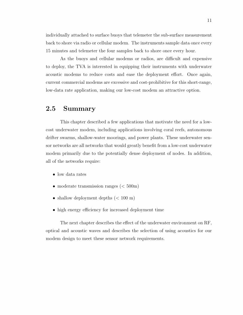
individually attached to surface buoys that telemeter the sub-surface measurement
back to shore via radio or cellular modem. The instruments sample data once every
15 minutes and telemeter the four samples back to shore once every hour.
As the buoys and cellular modems or radios, are difficult and expensive
to deploy, the TVA is interested in equipping their instruments with underwater
acoustic modems to reduce costs and ease the deployment effort. Once again,
current commercial modems are excessive and cost-prohibitive for this short-range,
low-data rate application, making our low-cost modem an attractive option.
2.5 Summary
This chapter described a few applications that motivate the need for a low-
cost underwater modem, including applications involving coral reefs, autonomous
drifter swarms, shallow-water moorings, and power plants. These underwater sen-
sor networks are all networks that would greatly benefit from a low-cost underwater
modem primarily due to the potentially dense deployment of nodes. In addition,
all of the networks require:
• low data rates
• moderate transmission ranges (< 500m)
• shallow deployment depths (< 100 m)
• high energy efficiency for increased deployment time
The next chapter describes the effect of the underwater environment on RF,
optical and acoustic waves and describes the selection of using acoustics for our
modem design to meet these sensor network requirements.

Chapter 3
Comparison or RF, Optical and
Acoustic Communication
Underwater
Present underwater communication systems involve the transmission of in-
formation in the form of radio frequency (RF) waves, optical waves, or acoustic
waves. Each of these techniques has advantages and limitations. This chapter ex-
plores the effect of the underwater environment on RF, optical and acoustic waves
and describes the rational for using acoustics for the UCSDModem design to meet
the requirements of the target applications described in Chapter 2.
3.1 Radio Frequency Waves
Radio frequency waves are electromagnetic waves in the frequency band
below 300GHz. An electromagnetic wave is a wave of energy having a frequency
within the electromagnetic spectrum (Figure 3.1) and propagated as a periodic
disturbance of the electromagnetic field when an electric charge oscillates or accel-
erates [30]. Underwater radio frequency communications have been investigated
since the very early days of radio [31], and had received considerable attention
during the 1970s [32], however few underwater RF systems have been developed
due to the highly conducting nature of salt water. This section discusses the effect
12

13
of conductivity, wavelength, and air/water interface on RF waves and describes
existing underwater systems that make use of RF waves.
10-16
10-14
10-12
10-10
10-8
10-6
10-4
10-2
100
102
104
106
108
1024
1022
1020
1018
1016
1014
1012
1010
108
106
104
102
100
X rays UV IR Microwave
Radio waves
FM AM Long radio waves
Frequency (Hz)
Wavelength (m)
Gamma rays
Figure 3.1: Electromagnetic Spectrum
3.1.1 Conductivity
Pure water is an insulator, but as found in its natural state, water contains
dissolved salts and other matter, which makes it a partial conductor. The higher
water’s conductivity, the greater the attenuation of radio signals that pass through
it. Propagating waves continually cycle energy between the electric and magnetic
fields, hence conduction leads to strong attenuation of electromagnetic propagating
waves [33]. Sea water has a high salt content and thus high conductivity varying
from 2 Siemens/meter (S/m) in the cold arctic region to 8 S/m in the Red Sea [34].
Average conductivity of sea water is considered to be 4 S/m whereas conductivity
of fresh water is typically on the order of a few mS/m [35].
Attenuation of radio waves in water increases both with increase in conduc-
tivity and increase in frequency. It can be calculated from the following formula
[34]:
α = 0.0173√fσ (3.1)
Where α is attenuation in dB/meter, f is the frequency in Hertz, and σ is
the conductivity in S/m.

14
Figure 3.2 shows attenuation as a function of frequency for sea water (4
S/m) and fresh water (0.01 S/m). Attenuation in sea water is very high and to
communicate at any reasonable distance, it is necessary to use very low frequencies.
However, the consequence of using very low frequencies is the need to use larger
antennas to capture the signal of larger wavelength.
100
101
102
10310
-2
10-1
100
101
102 RF Underwater Attenuation vs. Frequency
Frequency (KHz)
Atte
nuat
ion
(dB
per
met
er)
Sea WaterFresh Water
100
101
102
10310
0
101
102
103
104
105
106 RF Underwater Wavelength vs. Frequency
Frequency (KHz)
Wav
elen
gth
(m)
Sea WaterFresh WaterAir
Figure 3.2: RF Attenuation vs. Frequency in Fresh and Sea Water
3.1.2 Wavelength
Wavelength in water is calculated from the following formula [34]:
λ = 1000√
10/(fσ) (3.2)
Where λ is the wavelength in meters, f is the frequency in Hz, and σ is
the conductivity in S/m. Figure 3.3 plots wavelength vs frequency in air, sea

15
water (with conductivity 4 S/m), and fresh water (with conductivity 0.01 S/m).
A signal’s wavelength in air is considerably reduced underwater (especially in salt
water) leading to considerable differences in antenna engineering for terrestrial and
underwater communications.10
010
110
210
310-2
10-1
100
101
102 RF Underwater Attenuation vs. Frequency
Frequency (KHz)
Atte
nuat
ion
(dB
per
met
er)
Sea WaterFresh Water
100
101
102
10310
0
101
102
103
104
105
106 RF Underwater Wavelength vs. Frequency
Frequency (KHz)
Wav
elen
gth
(m)
Sea WaterFresh WaterAir
Figure 3.3: RF Wavelength vs. Frequency in Sea Water, Fresh Water, andAir
3.1.3 Air/Water Interface
As the attenuation loss in water is high, higher transmission distances may
be achieved by having the signal leave the water near the transmitter, travel via an
air-path, (where attenuation loss is low) and re-enter the water near the receiver.
However, as RF waves travel from air to water or water to air, there is a refraction
loss due to the change in the medium. This loss can be calculated via the following
formula [34]:
RefractionLoss(dB) = −20log(7.4586/106)√
10/(f/σ) (3.3)

16
Where f is the frequency in Hz, and σ is the conductivity in S/m.
Figure 3.4 illustrates refraction loss as a function of frequency for sea water
and fresh water. As frequency increases refraction loss decreases.
100
101
102
10320
30
40
50
60
70
80Air to Water Refraction Loss as a Function of Frequency
Frequency (KHz)
Atte
nuat
ion
(dB
)
Sea WaterFresh Water
Figure 3.4: Air to Water Refraction Loss as a Function of Frequency
Similar communications could be carried out underground depending on
the conductivity of the surrounding rock [33, 34].
3.1.4 Existing RF Systems
Because the conductivity of sea water poses severe attenuation to RF sig-
nals, only a few systems using RF underwater have been designed. Extremely low
frequency (ELF) radio signals have been used in military applications. Germany
pioneered radio communications to submarines underwater during World War II,
where their ”Goliath,” antenna was capable of outputting up to 1 to 2 Mega-Watt
(MW) of power, strong enough to send signals to submarines submerged in the In-

17
dian Ocean [36]. Later, a U.S. and Russian ELF system used 76Hz and 82Hz radio
frequency signals respectively to transmit a one-way ‘bell ring’ to call an individual
submarine to the surface to terrestrial radio for higher bandwidth communication
[37].
Until recently it was deemed impractical to use high frequency waves for
communication purposes. However, with new antenna designs, recent experiments
indicate that radio waves within the frequency range 1-20MHz can propagate over
distances up to 100 m, at rates beyond 1 Mbps, using dipole radiation with trans-
mission powers on the order of 100W [38, 39]. The antennas are very different
from those used for terrestrial communications [36, 38, 39]; instead of having direct
contact with seawater (as terrestrial antennas have direct contact with air), the
metal transmitting and receiving aerials are surrounded by waterproof electrically
insulating materials [38, 39] allowing an electromagnetic signal to be launched
from a transmitter into a body of seawater and picked up by a distant receiver.
100
101
102
10320
30
40
50
60
70
80Air to Water Refraction Loss as a Function of Frequency
Frequency (KHz)
Atte
nuat
ion
(dB
)
Sea WaterFresh Water
Figure 3.5: Wireless Fibre Systems SeaText Modem
The first commercial underwater radio-frequency (RF) modem in the world,
SeaText (Figure 3.5), was released by Wireless Fibre Systems [40] in September
2006. It can communicate over several tens of meters at a rate of 100bps. Wireless
Fibre Systems released a second RF modem, SeaTooth, which can support 1-100
Mbps within a 1 meter range [40].
Table 3.1, provided by [40] shows the possible rates and ranges of the
Wireless Fibre Systems RF modems in both sea and fresh water and their potential
applications.
18
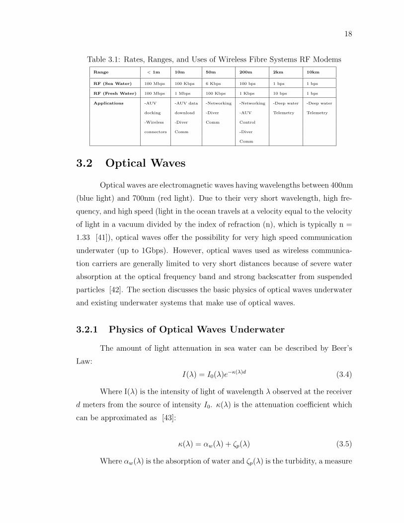
Table 3.1: Rates, Ranges, and Uses of Wireless Fibre Systems RF Modems
Range < 1m 10m 50m 200m 2km 10km
RF (Sea Water) 100 Mbps 100 Kbps 6 Kbps 100 bps 1 bps 1 bps
RF (Fresh Water) 100 Mbps 1 Mbps 100 Kbps 1 Kbps 10 bps 1 bps
Applications -AUV -AUV data -Networking -Networking -Deep water -Deep water
docking download -Diver -AUV Telemetry Telemetry
-Wireless -Diver Comm Control
connectors Comm -Diver
Comm
3.2 Optical Waves
Optical waves are electromagnetic waves having wavelengths between 400nm
(blue light) and 700nm (red light). Due to their very short wavelength, high fre-
quency, and high speed (light in the ocean travels at a velocity equal to the velocity
of light in a vacuum divided by the index of refraction (n), which is typically n =
1.33 [41]), optical waves offer the possibility for very high speed communication
underwater (up to 1Gbps). However, optical waves used as wireless communica-
tion carriers are generally limited to very short distances because of severe water
absorption at the optical frequency band and strong backscatter from suspended
particles [42]. The section discusses the basic physics of optical waves underwater
and existing underwater systems that make use of optical waves.
3.2.1 Physics of Optical Waves Underwater
The amount of light attenuation in sea water can be described by Beer’s
Law:
I(λ) = I0(λ)e−κ(λ)d (3.4)
Where I(λ) is the intensity of light of wavelength λ observed at the receiver
d meters from the source of intensity I0. κ(λ) is the attenuation coefficient which
can be approximated as [43]:
κ(λ) = αw(λ) + ζp(λ) (3.5)
Where αw(λ) is the absorption of water and ζp(λ) is the turbidity, a measure

19
of scattering caused by suspended particles. The scattering of water molecules and
absorption of particles may be neglected as they are small enough compared to the
parameters in Equation 3.5 [43].
The absorption of pure sea water, αw(λ), is given in Figure 3.6 [44, 45].
Sea water is composed primarily of H2O which absorbs heavily towards the red
spectrum, but also contains dissolved salts such as NaCl, MgCl2, Na2SO4, CaCl2,
and KCl that absorb specific wavelengths [46]. As seen in Figure 3.6, pure
seawater is least absorptive around 400-500nm, the blue-green region of the visible
light spectrum.
Figure 3.6: Absorption Coefficient of Pure Seawater [44, 45]
The scattering process of optical waves and the wavelength dependence of
underwater optical channels can be evaluated by the Mie scattering theory which
is valid for all possible ratios of particle diameter to wavelength [47]. Scattering in
the ocean is due to both inorganic and organic particles floating within the water
column. In coastal waters and continental shelf, inorganic matter contributes to
40-80% of the total scattering where in the open ocean scattering comes mainly
from organic particles (phytoplankton, etc.), [44]. According to the Mie theory,

20
light interacts with a particle over a cross-sectional area larger than the geometric
cross section of the particle when the light wavelength is similar to the particle
diameter. The scattering cross section area, Csca, defined as the total energy
scattered by a particle in all directions, as [47]:
Csca =
∫ 2π
0
∫ π0Iscar
2sinφdφdθ
I0(3.6)
where Isca is the scattered light intensity, I0 is the incident light intensity,
and r is the radius of the particle. The scattering cross section area is related to
turbidity as:
ζ =
∫Csca(x)p(x)dx (3.7)
where x is the particle diameter, Csca(x) is the scattering cross section
for particles with diameter x; and p(x) is the probability distribution function of
particle size.
Figure 3.7:
The Spectral transmittance over the upper 10m of water for Jerlov water
types I: extremely pure ocean water; II: turbid tropical-subtropical water;
III: mid-latitude water; 1-9: coastal waters of increasing turbidity [44, 48]

21
Figure 3.7 shows the effect of turbidity on optical transmittance across
the globe. In 1976, N. G Jerlov published the book Marine Optics that proposed
a system for classifying the clarity of the water [48]. This system divided the
globe’s sea water into two categories: oceanic (blue water) and coastal waters
(littoral zone). The oceanic group is subdivided into 3 groups; Type I-III and the
coastal group are subdivided into Types 1 through 9. Figure 3.7 shows the clarity
of oceanic water is much greater than the clarity of coastal water. Oceanic waters
are so clear that 10% of the light transmitted below the sea surface can reach a
depth of 90m. On the other hand, coastal waters, such as the Baltic sea (under
the category of coastal water 3) have large quantities of chlorophyll, causing highly
turbid water and a 10% transmittance depth of only 15 m [46].
3.2.2 Existing Optical Systems
Because water clarity plays such a significant role in determining whether
optical waves can be used for underwater communication, no commercial underwa-
ter optical modems have been developed. However, recent interests in underwater
sensor networks and sea floor observatories have greatly stimulated research inter-
est in short-range high-rate optical communication in water [42]. For example,
in [50], a dual mode (acoustic and optical) transceiver is used to assist robotic
networks where the optical transceiver achieves a data rate of 320 Kbps over a few
meters. The optical modem described by Schill et al achieves a range of 2 meters
for a rate of 57 Kbps [51]. In [52], an optical modem prototype is designed for
deep sea floor observatories and can operate up to 10 Mbps over 100 meters; and in
[53] a 1 Mbps LED-based communication system was demonstrated in a 12 foot,
1200 gallon tank. Furthermore, a recent study using Monte Carlo simulations over
seawater paths of several tens of meters indicates that optical communication data
rates greater than 1 Gbps can be supported and are compatible with high-capacity
data transfer applications that require no physical contact [54].
Recent experiments have also involved an acousto-optical hybrid approach
which uses laser to make sound underwater. In 2009, the U.S. Navy announced
the use of blue/green lasers to produce bubbles of steam that pop and create tiny,

22
220 decibel explosions [49]. The laser beam incident at the air-water boundary
is exponentially attenuated by the medium, creating an array of thermo-acoustic
sources relating to the heat energy and physical dimensions of the laser beam
in water, thus producing local temperature fluctuations that give rise to volume
expansion and contraction. The volume fluctuations in turn generate a propagating
pressure wave with the acoustic signal characteristics of the laser modulation signal
[55, 56, 57]. Controlling the rate of temperature fluctuations could provide a means
of communication.
3.3 Acoustic Waves
Acoustic waves are caused from variations of pressure in a medium. Due to
the greater density of water, they travel 4-5 times faster in water than they do in
air (traveling in water at an average of 1500 m/s - the speed of sound subject to the
water’s temperature, salinity and pressure), but are about 5 orders of magnitude
slower than electromagnetic waves (traveling near the speed of light as discussed in
Section 3.2). They have been widely used in underwater communication systems
due to the relatively low attenuation of sound in water. However, acoustic waves
can be adversely affected by absorption loss, spreading loss, ambient noise, and
severe multipath, which is discussed in this section.
3.3.1 Absorption Loss
The absorption of acoustic waves in sea water depends on the temperature,
salinity, and acidity of the sea water as well as the frequency of the sound wave.
The absorptive loss for acoustic wave propagation can be expressed as eα(f)d, where
d is the propagation distance and α(f) is the absorption coefficient of frequency f
[42]. For seawater, the absorption coefficient at frequency f in kHz can be written
as the sum of chemical relaxation processes and absorption from pure water [58]:
α(f) =A1P1f1f
2
f 21 + f 2
+A2P2f2f
2
f 22 + f 2
+ A3P3f2 (3.8)

23
Where the first term is the contribution from boric acid with f1 as its relax-
ation frequency, the second term is from the contribution of magnesium sulphate
with f2 and its relaxation frequency, and the third term is from the contribution
of pure water. The pressure dependencies are given by P1, P2, and P3 and A1,
A2, and A3 are constants. Figure 3.8 shows the variation in total absorption
vs. frequency for different oceans of different temperature, pressure, and pH [59].
Since α(f) increases with frequency, high frequency waves will be considerably
attenuated within a short distance while low frequency acoustic waves can travel
far.
1 December 2006 ASA-ASJ 4th Joint Meeting Honolulu HI 14
Boric, pH = 8, Atlantic
Boric, pH = 7.7, NE Pacific
MgSO4, p = 1 atm, 25 ºC
MgSO4, p = 103 atm, 25 ºC water (classical) 60 dB/km
water (actual) 60 dB/km
d
B/k
m
102 103 104 105 106 107 108
10-3
10-2
10-1
1
10
102
103
Hz
30x 10x
5x
10x
3x
Figure 3.8: Acoustic Absorption as a function of temperature, pressure, andpH [59]

24
3.3.2 Spreading Loss
The energy radiated from an omni-directional source spreads spherically
through a body of water. Since all the energy is not directed in a single direction
but in all directions, much of the energy is lost. This is called spreading loss. Note
that spreading loss is frequency independent. In deep water, the power loss caused
by spreading is proportional to the square of the distance. In shallow water, sound
is bounded by the surface and the sea floor resulting in cylindrical spreading. In
this case, sound power loss increases linearly with the distance from the source.
For a practical underwater setting, the spreading loss falls somewhere between
spherical and cylindrical spreading, with power loss proportional to dβ where β
is between 1 (for cylindrical spreading) and 2 (for spherical spreading) [60]. In
logarithmic terms, the classical equation for spreading loss is 10 log (dβ) [60] (see
Figure 3.9.
3.3.3 Noise
Ambient noise is defined as “the noise associated with the background din
emanating from a myriad of unidentified sources. Its distinguishing features are
that it is due to multiple sources, individual sources are not identified, and no one
source dominates the received field.” [61] Underwater sound is generated by a
variety of natural and man-made sources including breaking waves, rain, marine
life, bubbles, surface-ships, and military sonars. The primary source of ambient
noise can be categorized by the frequency of sound. In the frequency range of
20-500 Hz, ambient noise is primarily generated by distant shipping, in the range
500-100,000 Hz ambient noise is mostly due to spray and bubbles associated with
breaking waves. At frequencies above 100 KHz, thermal noise (noise generated by
the Brownian motion of water molecules) dominates.
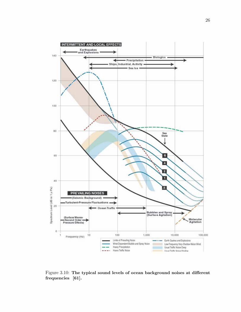
In 1962 Wenz and colleagues set out to measure background sounds in the
ocean and summarized them in a graph showing typical sound levels at different
frequencies [62]). (Figure 3.10 was adapted from [62] by [61]. The sound levels
in this graph are in dB relative to 1 µPa. Thus, when selecting a suitable frequency
band for communication, besides path loss, noise should be also considered [63, 64].

25
100
101
102
103
0
10
20
30
40
50
60
Range (m)
Lo
ss (
dB
)
Spreading Loss
Cylindrical Spreading
Spherical Spreading
Figure 3.9: Acoustic Spherical and Cylindrical Spreading Loss
26
Figure 3.10: The typical sound levels of ocean background noises at differentfrequencies [61].

27
3.3.4 Passive Sonar Equation
Given a source level, ambient noise level and equations for absorption and
spreading loss, one can use the passive sonar equation to determine the maximum
transmission distance achievable for a desired signal to noise ratio at the receiver.
The passive sonar equation is given by:
SNR(dB) = SL− TL−NL (3.9)
Where SNR is the desired signal to noise ratio at the receiver, SL is the
source level, TL is the transmission loss due to absorption and spreading, and
NL is the noise level attributed to the ambient noise level of the environment and
10∗log10(SignalBandwidth). Figure 3.11 shows the relationship between required
source level and range for four different SNR values at the receiver for a 40 kHz
carrier with 1kHz bandwidth and an ambient noise of 50 dB re 1 µPa (see Figure
3.10).

28
100
101
102
103
80
90
100
110
120
130
140
150
160
170Source Level vs. Transmission Distance for 40kHz carrier, 1kHz Bandwidth
So
urc
e L
eve
l (d
B r
e 1
μPa
)
Range (m)
SNR = 5dB
SNR = 10dB
SNR = 15dB
SNR = 20dB
Figure 3.11: Source Level vs. Transmission Distance for a 40 kHz carrier anambient noise of 50 dB re 1 µPa at various levels of SNR

29
3.3.5 Multipath
Underwater, there exist multiple paths from the transmitter to receiver, or
multipath. Two fundamental mechanisms of multipath formation are reflection at
the boundaries (bottom, surface and any objects in the water), and ray bending
(as sound speed is a function of temperature, salinity, and depth, rays of sound
always bend towards regions of lower propagation speed) [65]. Multipath due
to reflections off the surface and bottom is common in shallow waters whereas
multipath due to ray bending is common in deep waters. Understanding of these
mechanisms is based on the theory and models of sound propagation. Ray theory
and the theory of normal modes provide the basis for such propagation modeling.
Figure 3.12: Ray Trace for a 40kHz source with a 15 degree beam angle placedat 10 meters depth in a body of water 11 meters deep with a constant soundspeed of 1500 m/s
Bellhop is a commonly used, highly efficient ray tracing model. The un-
derwater acoustic propogation modeling software, AcTUP [66], can perform two-
dimensional Bellhop acoustic ray tracing for a given sound speed profile c(z) or a
given sound speed field c(r, z), in ocean waveguides with flat or variable absorb-
ing boundaries. Output options include ray coordinates, travel time, amplitude,

30
acoustic pressure or transmission loss. Figure 3.12 shows the Bellhop ray tracing
model for a 35kHz source with a 15 degree beam angle placed at 10 meters in a
body of water 11 meters deep with a constant sound speed of 1500 m/s.
Multipath can adversely affect communications because a large delay spread
(the time difference of arrival of the first and last path at the receiver) introduces
time dispersion of a signal, which causes severe inter-symbol interference. Typical
underwater channels may have a delay spread around 10ms, but occasionally delay
spread can be as large as 50 to 100ms [67] or as small as 3 ms [68]. The delay
spread of a receiver placed at 10m, 100m from the source in Figure 3.12 is only
300 microseconds.
3.4 Summary
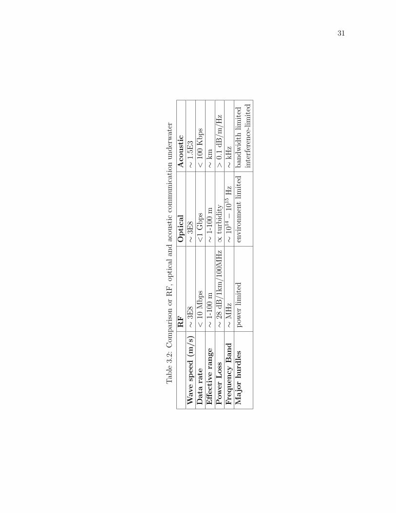
This chapter described the effect of the underwater environment on RF,
optical and acoustic waves. Table 3.2 (based on information in Tables II and III in
[42]) summarizes and compares the characteristics of radio, optical, and acoustic
communication underwater. All three physical wave fields have their own advan-
tages and limitations for acting as an underwater wireless communications carrier;
radio waves can provide high data rates, but are subject to strong attenuation by
the conductivity of sea water, optical waves provide even higher data rates, but
are subject to attenuation by the turbidity of sea water, acoustic waves provide
long transmission distances but support relatively low data rates and are subject to
multipath. As our sensor network applications (described in Chapter 2) require low
data rates and transmission distances greater than 100 meters, acoustics remains
the most robust and feasible carrier to date for wireless communication in these
underwater sensor networks. As acoustics have been widely used in underwater
communications and we have selected acoustics for our modem design, the next
chapter is devoted to describing and comparing exsiting commercial and research
underwater acoustic modems.
31
Tab
le3.
2:C
ompar
ison
orR
F,
opti
cal
and
acou
stic
com
munic
atio
nunder
wat
er
RF
Opti
cal
Aco
ust
icW
ave
speed
(m/s)∼
3E8
∼3E
8∼
1.5E
3D
ata
rate
<10
Mbps
<1
Gbps
<10
0K
bps
Eff
ect
ive
ran
ge
∼1-
100
m∼
1-10
0m
∼km
Pow
er
Loss
∼28
dB
/1km
/100
MH
z∝
turb
idit
y>
0.1
dB
/m/H
zFre
quency
Ban
d∼
MH
z∼
1014−
1015
Hz
∼kH
zM
ajo
rhurd
les
pow
erlim
ited
envir
onm
ent
lim
ited
ban
dw
idth
lim
ited
inte
rfer
ence
-lim
ited

Chapter 4
Existing Underwater Acoustic
Modems
As stated in the previous chapter, acoustic waves are widely used in un-
derwater communication systems due to the relatively low attenuation of sound in
water. Thus, quite a few companies and research groups have developed underwa-
ter acoustic modems for various undersea applications. This chapter describes and
compare existing commercial and recent research underwater acoustic modems to
better illustrate the novelty and applicability of the UCSDmodem design.
4.1 Commercial Modems
Commercial underwater acoustic modems are used by major offshore oil
companies, commercial survey companies, government agencies, universities and
defense contractors. This subsection discusses modems that are currently in pro-
duction and available for purchase. We focus on six commercial companies -
LinkQuest, Teledyne Benthos, TriTech International, Aquatec Group, EvoLogics,
and DSPComm, and the open architecture Micro-Modem developed at the Woods
Hole Oceanographic Institute (WHOI). In each case, we highlight the benefits, use
scenarios, and drawbacks of the modems.
LinkQuest claims to be the underwater acoustic modem market leader.
They produce a number of modems [69] ranging from the UWM1000 (a shallow
32

33
water, low power (2W transmit, 0.75 W receive) modem that can communicate up
to 350 meters with a data rate of 9600 to 19200 bps) to the UWM10000 (a full ocean
range and depth modem (40 W transmit, 0.8 W receive) that can communicate
up to 10 km with a data rate of 2500 to 5000 bps). The data rates vary primarily
as a function of the environment -a higher noise, higher multipath environment
having a lower data rate. As LinkQuest offers quite a range of modems, they can
be suited to many applications, however, their smallest and least expensive modem
(the UWM1000) costs $6500. LinkQuest also uses a proprietary signaling format
which causes concerns about interoperability between sensor nodes and inhibits
competition potentially increasing cost in the long term.
Teledyne Benthos manufactures modems that have been used in sub-sea
networks including the US Navy Seaweb program [10, 11], and the Front Resolving
Observation Network (FRONT) [9]. Their modems are marketed primarily for
point-to-point deep water vertical communication, e.g. from ocean floor directly
to the ocean surface [70]. They have demonstrated communication in over 1
kilometer of water at 10240 bits/second with no errors in ideal situations; however
they claim typical data rates less than 2400 bits/second. The modems are also
relatively power-hungry consuming 28-84 W transmit power and 0.7 W receive
power. Furthermore, the modems are quite expensive, costing over $7000.
TriTech International developed the Micron Data Modem [71] for small
remotely operated vehicle (ROV) communications. The Micron Modem appears
to be the smallest and lightest acoustic modem on the market thus making it
suitable for applications that have size and weight constraints (such as on board
small AUVs or ROVs). It is also half the cost of other acoustic modems on the
market with a retail cost of $3360. However, the Micron Modem has moderate
power consumption (7.92 W transmitting and 720mW receiving) for a maximum
range of 1km and low data rate (40 bps).
The Aquatec Group is a company that designs acoustic modems tailored
to suit the application of interest [72]. As part of their AquaModem long-range
series, they can offer modem configurations that provide a bit rate of 300-2000 bps
and a range of up to 20km. As part of their AquaModem500 short-range series,

34
they can offer modem configurations that provide a bit rate of 25-100bps, a range
of up to 250 meters. Modem costs start at $7600.
EvoLogics developed six underwater acoustic modems that make use of
their patented sweep spread carrier (S2C) underwater technology [73]. S2C was
designed to mimic a dolphin’s sound pattern and continuously spread the signal
energy over a wide range of frequencies so that the multipath components do not
interfere with each other. Their modems range from high speed modems (28kpbs)
for small to medium range applications (1000 meters) in shallow water to long
distance (8km), lower data rate (6.5kbps) in deep water. Costs once again vary
depending on modem configuration.
DSPComm produces the AquaComm, an underwater wireless modem that
provides the user with the ability to set the receive and transmit power thus offering
a low-power solution for short range applications [74]. The AquaComm has been
tested to a range of 3km and offers data rates of 100 or 480 bps depending on
the model. A 100 bps model costs $2800 and a 480bps model costs $3500 for the
electronics. The transducer and plastic case cost and additional $3100.
The Woods Hole Oceanographic Institute (WHOI) Micro-Modem [75] is
a popular open architecture alternative to the commercial solutions. It is user-
programmable and can support multiple instruments. It is currently used for com-
munication and navigation of autonomous underwater vehicles and autonomous
surface vehicles, buoy sensor telemetry and deep-water ocean observatories. The
Micro-Modem employs frequency-hopping frequency shift keying (FH/FSK) or
phase-shift keying (PSK) at the physical layer. FH/FSK is used in difficult chan-
nels, e.g. shallow water, littoral zones, communication to/from autonomous un-
derwater vehicles (AUVs), at low data rates (80bps). PSK is used for relatively
simple channels, e.g., deep water sea floor to surface, at higher data rates (up to
5400 bps). The modem electronics (without a water proof housing) cost $4900 with
an additional $1200 for the PSK co-processor. The transducer and cable assembly
for the modem costs $3200.
Table 4.1 compares modems from each of the above mentioned companies
in terms of operating frequency, transmit power, range, receive power, modulation

35
scheme, bit rate, and cost. For values not specified in the literature we denote
‘NS.’ The cost estimates were obtained from requesting a quote from each com-
pany (note that the costs may vary depending on the actual hardware components
selected for the modem including the transducer and housing). Operating frequen-
cies range from 8kHz - 78kHz (using lower frequencies to obtain longer ranges),
transmit powers vary from 2.5W - 80 W depending on the range, bit rate, and
modulation scheme, and bit rates range from 40-15000 bps. All modems make use
of proprietary commercial transducers which alone cost a few thousand dollars,
contributing a large portion to the overall cost of the modem. The last line of the
table denotes the properties of the UCSDModem design showing it provides less
range, lower bit rate and comparable power to most available commercial modems,
but costs an order of magnitude less. Note that the cost of the full UCSDModem is
solely for parts and does not include labor or market price, however, the parts cost
for the entire modem is still less than the cost of the commercial transducers used
in the other modem designs. Additional commercial modem comparisons may be
found in [76].

36
Tab
le4.
1:C
omm
erci
alU
nder
wat
erA
coust
icM
odem
Com
par
ison
Com
pany
Mod
em
Fre
qu
ency
Tx
Pow
er
Range
Rx
Pow
er
Mod
Bit
Rate
Cost
(kH
z)(W
)(k
m)
(W)
(bps)
($)
Aquat
ecA
QU
AM
odem
8-16
2010
0.6
DSSS
300-
2000
>76
00D
SP
Com
mA
quaC
omm
16-3
0va
ried
3va
ried
DSSS/O
FD
M48
066
00T
riT
ech
Mic
ronM
odem
20-2
47.
920.
50.
72D
SSS
4035
00W
HO
IM
icro
Modem
25<
501-
100.
23/
2F
SK
/PSK
80/5
400
8100
/940
0B
enth
osA
TM
885
16-2
128
-84
2-6
0.7
FSK
/PSK
140-
1536
072
00-1
1000
Evo
Log
ics
S2C
M48
/78
48-7
82.
5-80
10.
5S2C
1500
012
500
Lin
kQ
ues
tU
WM
2000
HN
S1.
50.
8N
SP
ropri
etar
y96
0070
00U
CSD
UC
SD
Modem
401.
3-7.
040
00.
42F
SK
200
350*
*Componentcost
estimate
only
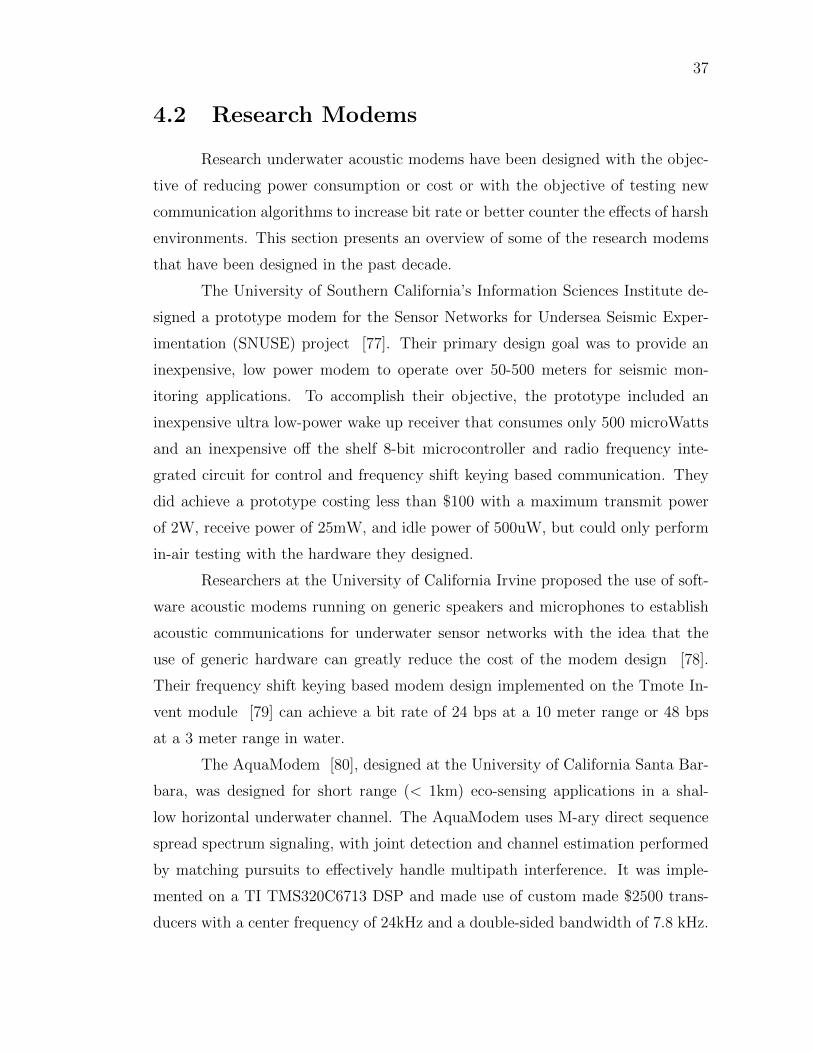
37
4.2 Research Modems
Research underwater acoustic modems have been designed with the objec-
tive of reducing power consumption or cost or with the objective of testing new
communication algorithms to increase bit rate or better counter the effects of harsh
environments. This section presents an overview of some of the research modems
that have been designed in the past decade.
The University of Southern California’s Information Sciences Institute de-
signed a prototype modem for the Sensor Networks for Undersea Seismic Exper-
imentation (SNUSE) project [77]. Their primary design goal was to provide an
inexpensive, low power modem to operate over 50-500 meters for seismic mon-
itoring applications. To accomplish their objective, the prototype included an
inexpensive ultra low-power wake up receiver that consumes only 500 microWatts
and an inexpensive off the shelf 8-bit microcontroller and radio frequency inte-
grated circuit for control and frequency shift keying based communication. They
did achieve a prototype costing less than $100 with a maximum transmit power
of 2W, receive power of 25mW, and idle power of 500uW, but could only perform
in-air testing with the hardware they designed.
Researchers at the University of California Irvine proposed the use of soft-
ware acoustic modems running on generic speakers and microphones to establish
acoustic communications for underwater sensor networks with the idea that the
use of generic hardware can greatly reduce the cost of the modem design [78].
Their frequency shift keying based modem design implemented on the Tmote In-
vent module [79] can achieve a bit rate of 24 bps at a 10 meter range or 48 bps
at a 3 meter range in water.
The AquaModem [80], designed at the University of California Santa Bar-
bara, was designed for short range (< 1km) eco-sensing applications in a shal-
low horizontal underwater channel. The AquaModem uses M-ary direct sequence
spread spectrum signaling, with joint detection and channel estimation performed
by matching pursuits to effectively handle multipath interference. It was imple-
mented on a TI TMS320C6713 DSP and made use of custom made $2500 trans-
ducers with a center frequency of 24kHz and a double-sided bandwidth of 7.8 kHz.

38
The modem was field tested in a shallow water coral reef and achieved ranges up
to 440 meters with a bit rate of 133 bps and an uncoded symbol error rate < 1%
[81].
Researchers at Kookmin University, Korea, designed an underwater acous-
tic modem that makes use of four small air transducers to communicate to other
nodes facing to the north, east, south, and west respectively and a fifth transducer
to communicate to a surface node. The design uses an ATmega128 as its micro-
controller unit which interfaces to an Arm PXA270 processor for medium access
layer (MAC) control. It operates at 30kHz and is capable of transmitting data up
to 5 kbps at ranges up to 30 meters [82].
Vasilescu et. al developed the AquaNode that is dually networked: optically
for point-to-point transmission at 330 kbps and acoustically for broadcast commu-
nication over ranges of hundreds of meters at 300 bps [83]. The acoustic modem
is are built around an Analog Device Blackfin BF533 fixed point DSP processor
and uses FSK modulation on a 30kHz carrier frequency. The nodes self-localize
and can be used to form static undersea networks. With all the nodes running at
full power, the battery provides 1-2 weeks of continuous operation.
Researchers at the University of Connecticut designed an orthogonal fre-
quency division multiplexing based modem on a TMS320C6713 DSP with the goal
of providing a higher data rate solution to other research modems [84]. The mo-
dem is capable of transmitting data at a raw data rate 3.1 kbps after rate 1/2
nonbinary LDPC coding and QPSK modulation. The modem has been tested in
water in a lab test tank, but has not been field tested, thus no range information is
available [85]. Researchers at Northwestern Polytechnical University in China also
designed a DSP based OFDM modem, implementing the design on a ADSP-TS101
and achieving an uncoded bit rate of 1kbps in a lake (range not specified) [86].
Sozer and Stojanovic developed a reconfigurable acoustic modem (rModem)
[87] designed to act as a physical layer prototyping platform. This platform in-
cludes a high processing power floating point DSP for the implementation of various
physical layer protocols and an FPGA that enables users to operate at any carrier
frequency and bandwidth within the 1kHz - 100kHz band by setting carrier coeffi-

39
cients, filter coefficients, and interpolation/decimation rates. The current rModem
design interfaces to a daughter card that can drive a Teledyne AT-408 transducer
that operates in the 9-14kHz band. Because the rModem is intended to be used
as a research tool rather than a commercial product, high processing power and
cost is tolerated. The rModem hardware and software operability was field tested
in Woods Hole, MA [88]. Similar to the rModem is the Universal Software Radio
Peripheral (USRP) underwater modem proposed to act as a solution for research
in implementing underwater modems and related signal processing [89].
Numerous other researchers have implemented communication algorithms
on a laptop computer and used commercially bought hardware to connect to the
laptop and conduct in-water experiments. Examples include OFDM based imple-
mentations [90, 91, 93, 94, 95, 96] and multiple-input, multiple-output (MIMO)
based implementations [97, 98, 99]. These designs are useful for examining the
capabilities of different modulation schemes, but are not designed for real-time
deployment.
Table 4.2 compares the described research modems in terms of platform,
modulation scheme, bit rate, and range. ‘NS’ denotes values not specified in the
literature. The last line of the table denotes the properties of the UCSDModem
design showing it provides similar rate and range performance to the AquaModem
and AquaNode, but was designed with low-cost as the primary design goal. The
UCSDModem design is also the only research modem design to implement FSK
on an FPGA.
4.3 Summary
This chapter described and compared existing commercial and recent re-
search underwater acoustic modems. The modem described in this thesis differs
from the commercial and research modems described above in that it focuses on
obtaining a cost-effective solution while still providing sufficient bit rate and range.
The design substitutes a commercial underwater transducer with a home-made un-
derwater transducer using inexpensive piezoceramic material and builds the rest

40
of the modem’s components around the properties of the transducer to extract as
much performance as possible. It is also the first design to implement frequency
shift keying on a field programmable gate array for underwater acoustic communi-
cation. The following 3 chapters describe the design details of each component of
the UCSDModem, including the low cost transducer, the analog transceiver and
digital transceiver.
41
Tab
le4.
2:R
esea
rch
Under
wat
erA
coust
icM
odem
Com
par
ison
Mod
em
Pla
tform
Mod
Bit
Rate
Range
BE
RC
om
ments
USC
MC
UF
SK
NS
NS
10−5
inai
rte
sts
only
(coded
)lo
w-p
ower
wak
eup
circ
uit
UC
IT
mot
eF
SK
125
10%
use
sge
ner
ichar
dw
are
uC
onn
DSP
OF
DM
6200
NS
NS
for
incr
ease
dbit
rate
tank
test
son
lyrM
odem
DSP
vari
edva
ried
vari
edN
Spro
toty
pin
gpla
tfor
mA
quaM
odem
DSP
DSSS
133
440
1%fo
rhig
hm
ult
ipat
hK
ook
min
MC
UN
S50
0030
NS
for
very
shor
tra
nge
AquaN
ode
MC
UF
SK
300
400
NS
dual
net
wor
ked
funct
ional
ity
UC
SD
FP
GA
FSK
200
400
4%fo
rlo
wco
st
Chapter 5
Transducer Design
This chapter describes the design of our low-cost transducer, an electro-
magnetic device responsible for converting electrical energy to mechanical energy
(sound pressure) and vice versa. We first describe the selection of the transducer’s
piezoceramic based on its type and geometry. We then describe our transducer
construction techniques including the selection of wiring, potting compound, and
mold. We finally describe the procedures used to measure the electromechanical
properties of our homemade transducer and present the experimentally determined
electromechanical properties that are used to govern the rest of the UCSDModem
design.
5.1 Piezo Ceramics
In 1880, Jacques and Pierre Curie discovered that certain naturally occur-
ring crystalline substances (such as quartz) exhibit an unusual characteristic: when
subjected to a mechanical force, the crystals became polarized and when exposed
to an electric field the crystals lengthened or shortened according to the polarity
and in proportion to the strength of the field. These behaviors were labeled the
piezoelectric effect and the inverse piezoelectric effect, respectively [100, 103, 102].
In the 20th century, researchers began to manufacture synthetic materials
that exhibit the piezoelectric effect using polycrystalline ceramics or certain syn-
thetic polymers. These materials are relatively inexpensive to manufacture, phys-
42

43
ically strong, and chemically inert. Common compositions include lead zirconate-
titanate and barium-titanate [100]. The type of the ceramic and its geometry
affect the ceramic’s piezoelectric properties and are described in more detail in the
following subsections.
5.1.1 Type
Although several standards exist, in the US, piezoceramics are popularly
classified into 6 types created by DOD-STD-1376A [104] which was replaced by
MIL-STD-1376B [105] in 1995 and discontinued in 1999. Although the standard
is no longer officially used, most ceramics manufactures still use it as a guideline
and have options of their product that comply with the standard. If a ceramic is
chosen from one type, it will be very similar in properties to other ceramics in the
same type. The typical properties of each type are [105]:
• TY PE I- A modified lead zirconate-titanate composition generally recom-
mended for medium- to high-power acoustic applications. Its ”resistance” to
depoling at high electric drive and/or mechanical stress makes it suitable for
deep-submersion acoustic applications.
• TY PE II- A lead zirconate-titanate composition modified to yield higher
charge sensitivity but one that is not suitable for high electric drive due to
dielectric heating. This material is more suitable for passive devices such as
hydrophones. Advantages also include better time stability.
• TY PE III- Similar to Type I but greatly improved for use at high electric
drive because of lower losses. Its field dependency of dielectric and mechani-
cal losses is substantially reduced. However, at low to moderate electric drive
levels Type I material may actually be a better choice because of greater elec-
tromechanical activity.
• TY PE IV - A modified barium-titanate body for use in moderate electric-
drive applications. It is characterized by lower piezoelectric activity and lower
Curie temperature than any of the lead zirconate-titanate compositions.

44
• TY PE V - A composition intermediate to Types II and VI and thus to be
used accordingly.
• TY PE V I- Similar to Type II with higher charge sensitivity and dielectric
constant, at the expense of a reduced Curie temperature.
The six types of ceramics can be further lumped into two very general
groups: hard and soft ceramics. Hard ceramics have low dielectric and mechani-
cal loss and are generally better at producing a signal whereas soft ceramics have
large dielectric losses, low mechanic quality factors, and poor linearity, but are
generally better at receiving a signal [100, 101]. Soft ceramics produce large dis-
placements and wider signal bandwidth, but they exhibit greater hysteresis and are
more susceptible to depolarization [100]. Either of these ceramics is still capable of
producing and receiving signals regardless of which group it is in because of piezo-
electric reciprocity. For underwater network communication where one transducer
is used for transmitting and receiving for cost effectiveness, a piezoelectric element
that is good at doing both is desired.
We selected to use a ‘hard’ modified Navy Type I ceramic due to its low
dielectric and mechanical loss and high electromechanical coupling efficiency mak-
ing it suitable as both a transmitter and receiver. Also, ceramics manufactured
from formulations of lead zirconate-titanate (PZT) are the most widely used be-
cause they exhibit greater sensitivity and higher operating temperatures, relative
to ceramics of other compositions [102]. A typical Type I PZTs can experience up
to 12 Vpp AC per .001 inches wall thickness without much effect to its electro-
mechanical properties [106]. A thickness of 0.1 inches (2.54 mm) gives a maximum
voltage of 1200 Vpp or 425 Vrms.
5.1.2 Geometry
After selecting the type of ceramic necessary for the application, the geom-
etry selection is the next important step. The cost of the PZT element can vary
greatly and is significantly affected by geometry. Not only are some shapes harder
to make, more intricate shapes make poling the ceramic more difficult as well.

45
Element geometry and polarization direction determine the radiated direction of
acoustic signals as well as the electro-mechanical properties of the ceramic element
itself, such as resonance frequency, capacitance, generated voltage under load, and
displacement. Exactly how they are affected depends on the geometry selected.
Simplified equations for commonly used shapes can be found on many ceramic
manufactures’ websites [101, 102]. Geometry- independent properties include the
electromechanical coupling coefficient, piezoelectric constants, dielectric constant,
curie temperature, and dissipation factor which depend on the material.
For underwater communication, ceramics are usually omni-directional in
the horizontal plane to reduce reflection off the surface and bottom [103]. A radial
expanding ring provides 2D omni directionality in the plane perpendicular to the
axis and near omni directionality in planes through the axis only if the height
of the ring is small compared to the wavelength of sound being sent through the
medium. Note, if the ring is too tall, extension along the axis and bending modes
of the ring may become a problem [103].
A radial expanding ring ceramic element can be made of several ceramics
cemented together, providing greater electromechanical coupling, power output,
and electrical efficiency than one-piece ceramic rings. The piezoelectric constant
and coupling coefficient are approximately double that of a one-piece ceramic ring
[103]. They work better because the polarization can be done in the direction of
primary stresses and strains along the circumference. However, these are much
more difficult to manufacture and are therefore much more expensive than a one-
piece radial expanding piezoelectric ceramic.
Thus, a one piece modified Type I ring transducer with radial resonance
mode, 26 mm outer diameter, 22 mm inner diameter, and 2.54 mm wall thickness
was selected. Specifically, part SMC26D22H13SMQA from Steiner and Martins,
Inc. [108] was purchased for approximately $10 per element with no minimum
purchase. This is much less than many other piezoelectric manufactures charge
for ceramics with very similar geometry and electro-mechnical properties. Much of
the cost difference stems from the difficulty of manufacturing PZTs with consistent
properties under tight tolerances. Many piezoceramics for underwater communi-

46
cation are being used for oil and military use where they must comply with tight
specifications and operate under extreme conditions. These extreme conditions in-
clude deep ocean and long range operation. Thus many companies cater towards
this market selling high quality parts that are not necessarily needed for short-range
underwater communication research. In this context lower quality does not mean
lower performance, but a looser control on tolerances and increase in availablitly
to drive down costs.
For a single radial expanding ceramic ring, the resonance frequency occurs
when the circumference approximately equals the operating wavelength [103]. The
resonance frequency and anti-resonance frequency occur at minimum and maxi-
mum impedances, respectively [103, 107]. In air, the resonance frequency is about
41 kHz for every inch in diameter; for the ring made of several ceramics cemented
together, in the case that there is not inactive material (such as electrodes or ce-
ment), the resonance frequency is approx 37 kHz for every inch [103]. If the ring
is too tall, problems with length extensional and bending modes of vibration may
be experienced. The bandwidth of the ceramic is broader if the thickness is much
smaller than the radius [103]. The SMC26D22H13SMQA has an outer diameter
of 26mm (approx 1 in) and has a nominal resonance frequency of about 43 kHz.
Steiner and Martins, Inc. specifies that the ceramic ring has a nominal resonance
frequency of 43kHz +/- 1.5kHz.
5.2 Transducer Construction
Although the piezoelectric element is a key component of the transducer,
there are other aspects to manufacturing a transducer that are important to its
performance. Attaching electrical leads, reducing unwanted acoustic radiation,
and potting the piezoceramic should be paid special attention. Figure 5.1 depicts
our raw piezoceramic, transducer before potting, and fully potted transducer.

47
(a) (b) (c)
Figure 5.1:
(a) Raw PZT , (b) Prepotted Transducer , (c) and Potted Transducer
5.2.1 Wiring
Using shielded cables to attach to the ceramic will greatly enhance the
performance of the transducer. Unshielded wires can act as antennas and pick up
much unwanted electromagnetic noise that can bury small signals received by the
transducer. When soldering to the ceramic’s electrodes, care should be taken to
prevent contact of the soldering tip to the ceramic for more than a few seconds.
Heating the ceramic above its curie temperature will damage its electromechanical
properties. If possible, the soldering iron’s temperature should be also be adjusted
accordingly. Solder with 3% silver is recommended by Steminc [108].
5.2.2 Potting
The piezoelectric ceramic needs to be encapsulated in a potting compound
to prevent contact with any conductive fluids. Urethanes are the most common
material used for potting because of their versatility. The most important design
consideration is to find a urethane that is acoustically transparent in the medium
that the transducer will be used; this is more important for higher frequency or
more sensitive applications where wavelength and amplitude is smaller than the
thickness of the potting material. Many urethane manufactures do not know the
acoustical properties of their urethanes. However, information on similarities to
water’s acoustical properties is becoming easier to find. Generally, similar density

48
provides similar acoustical properties. Mineral oil is another good way to pot the
ceramics because it is inert and has similar acoustical properties to water. Some
prefer using mineral oil to urethane because it is not permanent. However, the oil
still needs to be contained by something, which is often a urethane tube. A two-
part urethane potting compound, EN12, manufactured by Cytec Industries [109]
was selected as it has a density identical to that of water, providing for efficient
mechanical to acoustical energy coupling.
Creating a transducer by potting the ceramic shifts its resonant frequency
due to the additional mass moving immediately around the transducer. The ex-
tent of the shift depends on the type, age, and amount of potting as well as the
temperature and mixing method of the compound. Having tight control over these
variables to ensure exact reproducibility requires expensive equipment. To keep
costs low, we used the following simplistic potting method.
As urethanes are toxic, when potting the ceramic, avoid touching or inhaling
the fumes of the urethane compound as specified by the MSDS provided by the
manufacture. Urethanes must have the correct ratio of both parts. Adding more
of one will not help it cure faster, will change its physical properties, and many
times will prevent it from fully curing at all. A scale was used to measure the exact
proportions of the two part compound and hand-poured the parts into a plastic
container for mixing. Larger batches will help with keeping mixing ratios more
consistent between separate batches.
Urethanes are very susceptible to moisture absorption. The moisture cre-
ates bubbles within the urethane and are undesired because they absorb acoustic
waves propogating from the piezoceramic. Much of the moisture is introduced
during mixing. Using plastic or metal spoons and containers over paper or wooden
ones during mixing will reduce the amount of bubbles that appear in the cured
urethane. Unmixed urethane in opened containers are often stored in metal cans
and covered with a blanket of nitrogen to reduce moisture absorption [110].
Although this was not done on our own transducer, placing a vacuum on
the urethane mixture while curing will cause many of the bubbles to enlarge and
rise out of the curing liquid. In addition, the curing urethane can subsequently

49
be placed under pressure to reduce the remaining bubbles’ size. Higher vacuums
and putting unmixed urethane components into a vacuum separately may cause
boiling of certain chemicals that need to remain in the liquid components in order to
cure [110]. Again, processing parameters in the urethane’s technical specifications
should be followed for best results. Tips on making molds, and other potting tips
can be found at [111].
A tennis ball with a hole cut in it and an ABS pipe cap with holes drilled in
it were glued together using silicone and used as our transducer’s mold. The ABS
cap was only used for mounting. Mixed and uncured urethane was poured into the
mold through the holes in the ABS cap. After the urethane was fully cured the
tennis ball and silicone were removed.
5.2.3 Reducing Unwanted Acoustic Radiation
For a ring transducer with radial acoustic radiation, only pressure waves
from the outer surface are desired. Pressure waves formed at the top, bottom, and
inner surfaces create pressure waves that are out of phase with those formed by
the outer surface leading to destructive interference in the far field regime. For
this reason many cylindrical transducers are constructed with air or other acoustic
damping material within the piezoceramic. Cork was used for our transducer (as
shown in Figure 5.1(b). Discs of cork with an adhesive backing were placed on
the top and bottom surfaces of the piezoceramic as well, to absorb radiation from
these surfaces.
At depth, having a pocket of air in the transducer can be problematic. For
deep water cylindrical transducers, end caps are often made of metal plates or
curved ceramics to withstand pressures at depth; to prevent clamping sometimes
a rod is run along the cylinder’s axis [103]. The end caps should be acoustically
isolated from the piezoelectric ceramic. If the circumferential stress (the quantity
of pressure multiplied by radius over thickness) is above 10000 to 15000 psi the
piezoceramic’s parameters will start to deteriorate [103]. The pressure at 100m
depth is only about 150 psi above the pressure at sea level. Free flooded rings are
still used for some deep water circumstances.
50
5.2.4 Material Costs
The material cost of each of our transducers was less than $45 excluding the
ABS mounts which are not necessary. The Steminc PZT (SMC26D22H13SMQA)
cost $10 each with no minimum order. The Cytec EN12 potting compound cost
$150 per quart. A 100ft roll of shielded cable (C1202-100-ND) from Digikey
cost $130, and adhesive backed quarter and eight inch thick 1x3 feet cork sheets
(9487K51 and 9487K54) cost $6 and $13 respectively. The mold’s costs are rela-
tively low as well; tennis balls can be purchased for less than $2 per ball.
The next section describes the procedures used to determine the electrome-
chanical properties of the homemade transducer.
5.3 Calibration Procedures
The calibration of a transducer consists of the determination of its electro-
mechanical response as a function of frequency; namely its transmitting voltage
response (TVR) and its receiving voltage response (RVR). The TVR is defined as
the sound pressure level experienced at 1m range, generated by the transducer per
1 V of input voltage as a function of frequency. The RVR is a measure of the voltage
generated by a plane wave of unit acoustic pressure at the receiver and is a function
of frequency. The units of the transmitting response are typically expressed in
dB/1uPa/m and the units of the receiving response are typically expressed in
dB/1V/uPa. Although numerous calibration procedures exist [112], the following
subsections describe the two most commonly used methods: comparison method
and reciprocity method.
5.3.1 Comparison Method
The comparison method is the simplest transducer calibration procedure
wherein the output of the unknown transducer is compared with that of a pre-
viously calibrated reference transducer. The unknown and reference transducers
are placed in a tank of water at known separation (typically 1 m). To obtain the
RVR, the reference transducer sends sinusoidal signals of a known duration across

51
the desired frequency range and the unknown transducer collects the sinusoidal
signals over the same duration at each frequency. The collected data represent
the combination of the transmitting response of the reference transducer plus the
receiving response of the unknown transducer and the effects of attenuation at the
seperation distance. The RVR may be calculated using the following equations :
D = 20log10(VreceiverVtransmitter
) (5.1)
RV R = Dfromref + TV Rref + A (5.2)
where Vreceiver is the average amplitude voltage of the receiver over the
known duration, Vtransmitter is the average amplitude voltage of the transmitter over
the known duration and A is the attenuation of the signal due to the seperation
distance.
To obtain the TVR, the unknown transducer sends sinusoidal signals of
reference duration across the desired frequency range and the reference transducer
collects the sinusoidal signals over the reference duration at each frequency. The
collected data represents the combination of the transmitting response of the un-
known transducer plus the receiving response of the reference transducer and the
affects of attenuation at the seperation distance. The RVR may similarly be cal-
culated as:
TV R = Dto ref −RV Rref + A (5.3)
5.3.2 Reciprocity Method
As the reciprocity method does not require the use of a reference transducer,
it is a useful and often used calibration technique. The reciprocity technique was
first introduced by MacLean [113] and applied to underwater sound by Ebaugh
and Meuser [114]. The self-reciprocity technique was later described by Simmons
and Urick [115]. The reciprocity method is based off the electroacoustic reciprocity
principle which relates current and open-circuit voltage on the electrical side to the

52
diaphragm velocity and impressed force on the acoustical side of an electroacoustic
device:
|E||v|
=|F ||I|
(5.4)
Where E is the electric voltage, I is the electric current, v is the velocity
on the diaphragm and F is the force of the diaphragm. This expression can be
used to calibrate a transducer by relating velocity v to the pressure produced at a
distance when the transducer is acting as a transmitter and by relating the force
F to the incident sound wave when the transducer is acting as a receiver. The
relationship depends on whether the transducer generates spherical, cylindrical, or
plane waves [112].
For a cylindrical transducer, the acoustic pressure at distance r can be
shown to be [112]:
Pr = πρav
(cf
r
)1/2
(5.5)
where ρ is the density of water, a is the radius of the cylinder, v is the
surface velocity of the cylinder, c is the velocity of sound and f is the carrier
frequency. If the transducer acts as a receiver, the force exerted upon it by an
incident sound field of pressure Pi will be [112] :
F = APi = 2πaLPi (5.6)
where A is the face area of the cylinder and L is the length of the cylinder.
Inserting into the reciprocity relationship 5.4 we obtain [112]:
E
Pi2πaL=PrI
(r
cf
)1/21
πρa(5.7)
Writing equation 5.7 as the relationship between the receiving response M
= E/Pi and the transmitting response S = Pr/I we obtain [112]:
Jc =M
S=
2L
ρc
(cr
f
)1/2
(5.8)

53
The ratio Jc was first derived by Bobber and Sabin [116] and is called the
cylindrical wave recipirocity parameter. It can be empirically measured.
Using self-reciprocity, Pi = Pr assuming the pressure field incident on the
receiver is the same as that generated by the transmitter. The receiving response
may then be measured as [115]:
M =
(JcErI
)1/2
=
(JcErZ
Et
)1/2
(5.9)
where the current I equals the known transmitted voltage, Et, divided by the
measured impedance Z, and Er is the measured received voltage.
5.4 Experimental Measurements
Due to its simplicity, we made use of the comparison method to calibrate
the homemade transducers. We suspended both the homemade transducer and
reference transducer, a spherical ITC 1042 [118], 0.18 meters apart in the middle
of a 3 meter deep, 2 meter wide cylindrical test tank filled with salt water. Burst
signals of duration 2ms, across frequencies in 1kHz increments were sent from the
reference transducer to the homemade transducer and vice versa. Signals were sent
and collected via LabView. Figures 5.2 and 5.3 show the TVR and RVR of the ITC
transducer, a Marport transducer [117] (a directional commercial transducer), and
the homemade transducer (T1). As expected, the gain of the Marport (directional)
transducer is higher than that of transducer T1 as it can concentrate its energy in
one direction. The gain of transducer T1 is higher than that of the ITC transducer
due to the larger physical size of its ceramic.
Adding the TVR and RVR gives a quantity known as the ‘Figure of Merit’
which gives an indication of the transducer’s best operating frequencies when acting
as both a transmitter and receiver. Figure 5.4 shows the Figure of Merit calculated
from the Lab View data indicating an operating frequency range around 40kHz for
transducer T1. The peaks and valleys of the Figure of Merit can be attributed to
constructive and destructive interference caused by reflections off the sides of the
small calibration tank.

54
13
5
14
0
14
5
15
0
B re microPa/V @1mT
ran
sd
uce
r T
ran
sm
itte
r V
olta
ge
Re
sp
on
se
Marp
ort
(S
pec)
ITC
1042 (
Spec)
T1 (
LabV
iew
)
12
5
13
0
30
35
40
45
50
55
dB
Fre
qu
en
cy (
kH
z)
Fig
ure
5.2:
Tra
nsd
ucer
Tra
nsm
itte
rV
olt
age
Resp
on
se

55
19
5
-19
0
-18
5
-18
0
-17
5
dB re V/microPaT
ran
sd
uce
r R
ece
ive
r V
olta
ge
Re
sp
on
se
Marp
ort
(S
pec)
ITC
1042 (
Spec)
T1 (
LabV
iew
)
-20
5
-20
0
-19
5
30
35
40
45
50
55
Fre
qu
en
cy (
kH
z)
Fig
ure
5.3:
Tra
nsd
ucer
Receiv
er
Volt
age
Resp
on
se

56
-62
-52
-42
2030
4050
6070
8090
100
dB
T1 F
igur
e of
Mer
it
-82
-72
Freq
uenc
y (k
Hz)
Fig
ure
5.4:
Tra
nsd
ucer
Fig
ure
of
Meri
t

57
5.5 Summary
This chapter described the design of our low-cost transducer, its ceramic
type and geometry, its potting compound and procedure, and its electro-mechanical
properties. The low-cost transducer costs ∼ $40, is omni-directional in the hori-
zontal plane, operates in a narrow frequency band around 40kHz, and has a source
level of about 140 dB re 1uPa @ 1m. The next chapter describes the UCSD-
Modem’s analog transceiver which was designed to operate in the transducer’s
operating frequency range.
The text of Chapter 5, is currently being prepared for submission for pub-
lication of the material. The dissertation author was a co-primary researcher and
author (with Kenneth Domond). Ryan Kastner and Don Kimball directed and
supervised the research which forms the basis for Chapter 5.

Chapter 6
Analog Transceiver Design
The analog transceiver consists of a power amplifier, a power management
circuit, an impedance matching circuit, and a pre-amplifier (Figure 6.1). The
power amplifier is responsible for amplifying the modulated signal from the digital
hardware platform. It sends the signal to the power management circuit which
further amplifies the signal to a power level that matches the actual distance be-
tween the transmitter and receiver. The power management circuit then sends
the amplified signal to the impedance matching circuit, which is matched to the
transducer’s resonance frequency, so that the signal may be transmitted efficiently
to the water. The pre-amplifier amplifies the signal that is detected by the trans-
ducer so that the digital hardware platform can effectively demodulate the signal
and analyze the received data. This chapter describes the design of the power am-
plifier, power management circuit, impedance matching circuit, and pre-amplifier
of the analog transceiver.
6.1 Power Amplifier Design
When designing the power amplifier we considered the following require-
ments:
• The amplifier should provide a linear, undistorted output over a relatively
wide bandwidth (10 - 100kHz) to allow for use with a variety of underwater
58

59
Figure 6.1: Analog Transceiver
transducers
• The amplifier must be power efficient (especially for large output power) as
a deployed modem must be powered from batteries
Power amplifiers are classified according to their circuit configurations and
methods of operation into different classes such as A, B, AB, C, D, G and H.
These classes range from entirely linear with low efficiency to entirely non-linear
with high efficiency [119]. An amplifier is said to be linear if it preserves the details
of the signal waveform, that is:
V0(t) = AVi(t) (6.1)
The amplifier is said to be efficient if it can convert the majority of the
dc power of the supply into the signal power delivered to the load. Efficiency, is
defined as:
efficiency =signal power delivered to load
DC power supplied to output circuit(6.2)

60
To meet our design requirements, we wished to design a power amplifier
that was both linear and efficient. We considered the characteristics of the most
common amplifier classes (A, B, AB, and D). The following material was gathered
from [120, 121, 122].
A Class A amplifier consists of a single transistor for its output stage con-
ducting over the whole of the input cycle such that the output signal is an exact,
scaled-up, replica of the input and thus completely linear. However, because the
amplifier is continuously conducting, Class A amplifiers are not very efficient, hav-
ing a theoretical maximum efficiency of 50% (with typical operation at 10-25%
efficiency). A typical Class A input / output characterisitic is shown in Figure 6.2.
Figure 6.2: Class A Amplifier Input/Output Characteristic
Unlike a Class A amplifier, a Class B amplifier consists of two complimen-
tary transistors to handle both halves of the waveform. Each amplifying device
conducts for only half the sinusoidal cycle and neither device conducts when there
is no input, thus increasing the efficiency of the amplifier. Class B amplifiers typ-
ically have an efficiency of about 50%, but have some issues with linearity at the
crossover point, due to the time it takes to turn one transistor off and turn the
other transistor on. A typical Class B input / output characterisitic for one of its

61
transistors is shown in Figure 6.3.
Figure 6.3: Class B Amplifier Input/Output Characteristic for one transistor
Figure 6.4: Class AB Amplifier Input/Output Characteristic for onetransistor
The Class AB amplifier is a compromise between the Class A and Class B
configurations and is currently one of the most common types of power amplifiers

62
in existence. Like a Class B amplifier, the Class AB amplifier consists of two com-
plementary transistors, but unlike the Class B amplifier, both devices are allowed
to conduct at the same time, but just a small amount near the crossover point.
Thus each device conducts for more than half a cycle but less than a whole cycle,
overcoming the inherent non-linearity of Class B designs without the inefficiencies
of a Class A design. Efficiencies for Class AB amplifiers are typically 50% with a
theoretical maximum of 72%. A typical Class AB input / output characterisitic
for one of its transistors is shown in Figure 6.4.
The Class D amplifier is a ‘switching amplifier.’ The basic Class D amplifier
consists of a comparator, a switching stage (typically two MOSFET transistors)
and a low pass filter. A block diagram of a basic Class D amplifier is shown in Fig-
ure 6.5. The input signal is compared to a sawtooth waveform (of higher frequency
than the highest frequency component of the input signal) and the output signal
of the comparator goes high when the input signal is higher than the sawtooth
waveform. The output of the comparator drives two transistors which operate
as switches creating a pulse width modulated waveform. The switches are either
fully on or fully off, significantly reducing the power losses in the output devices.
The low pass filter removes inaccurate spectral components resulting in an output
signal that is an amplified replica of the input (although not completely linear).
Efficiencies of 90-95% are possible.
As we desired a highly linear amplifier (in the range of 10-100kHz) with
high power efficiency (especially for large power outputs) we designed a unique
architecture that consists of a Class AB and a Class D amplifier working in parallel
(Figure 6.6).
The primary amplifier is a highly linear Class AB amplifier that provides a
highly linear voltage gain of 27 across input voltages and frequencies (see Figure
6.7). The output of the Class AB amplifier is connected to current sense circuitry
that in turn controls the secondary amplifier, which is a Class D switching amplifier.
The Class D amplifier is inherently nonlinear, but when working in tandem with
the Class A/B amplfier, it produces a linear output for input voltages greater than
500 mVpp across frequencies (see Figure 6.8). The Class D amplifier provides high

63
Low Pass Filter
Switching Controller
And Output Stage
Triangle Wave Generator
Input
Figure 6.5: Block diagram of a basic switching or PWM (Class-D) amplifier
Output
Input
Class AB Linear
Amplifier
Current Sense and Switcher
Controller
+
Class D Switching Amplifier
DC ZL
ZS
VL
+
-
Figure 6.6: Block diagram of the power amplifier design making use of a classAB and class D amplifier to achieve linearity and efficiency
power efficiency to the complete amplifier for large power outputs (where the load
resistance is below 15 ohms) but must be turned off for lower power outputs where
its efficiency drops below that of the Class A/B amplifier alone.

64
2022242628303234
020
040
060
080
010
00
Gain
Inpu
t Vo
ltag
e (m
V)
Clas
s A
B Li
near
ity
10kH
z
20kH
z
30kH
z
40kH
z
50kH
z
60kH
z
70kH
z
80kH
z
90kH
z
100k
Hz
202530354045
100
200
300
400
500
600
700
800
900
1000
Gain
Inpu
t Vo
tlag
e (m
V)
Com
plet
e Tr
ansm
itte
r Li
near
ity
10kH
z
20kH
z
30kH
z
40kH
z
50kH
z
60kH
z
70kH
z
80kH
z
90kH
z
100k
Hz
Fig
ure
6.7:
Cla
ssA
BP
ow
er
Am
plifi
er
Lin
eari
ty

652022242628303234
020
040
060
080
010
00
Gain
Inpu
t Vo
ltag
e (m
V)
Clas
s A
B Li
near
ity
10kH
z
20kH
z
30kH
z
40kH
z
50kH
z
60kH
z
70kH
z
80kH
z
90kH
z
100k
Hz
202530354045
100
200
300
400
500
600
700
800
900
1000
Gain
Inpu
t Vo
tlag
e (m
V)
Com
plet
e Tr
ansm
itte
r Li
near
ity
10kH
z
20kH
z
30kH
z
40kH
z
50kH
z
60kH
z
70kH
z
80kH
z
90kH
z
100k
Hz
Fig
ure
6.8:
Com
ple
teP
ow
er
Am
plifi
er
Lin
eari
ty

66
0102030405060708090100
Efficiency (%)
Am
plifi
er E
ffic
ienc
y
50 k
Hz
Com
plet
e
30kH
z Co
mpl
ete
50 k
Hz
Clas
s A
/B
30 k
Hz
Clas
s A
/B
0102030405060708090100 0.
0010
.00
20.0
030
.00
40.0
050
.00
60.0
070
.00
80.0
090
.00
100.
00
Efficiency (%)
Load
(ohm
s)
Am
plifi
er E
ffic
ienc
y
50 k
Hz
Com
plet
e
30kH
z Co
mpl
ete
50 k
Hz
Clas
s A
/B
30 k
Hz
Clas
s A
/B
Fig
ure
6.9:
Pow
er
Am
plifi
er
Pow
er
Effi
cie
ncy

67
6.2 Power Management Circuit
The power management circuit is provided to adjust the output power of
the transceiver in real-time to match the actual distance between transmitter and
receiver. The power management circuit takes the output of the power amplifier
and further amplifies it to one of five power levels depending on how far the mo-
dem must transmit the signal. This is enabled through five different outputs at
the taps on the secondary coil of the transformer (Figure 6.10). The number of
windings on the secondary coil (N) divides the effective resistance of the load by
N2 thus increasing the power. The different transformer taps are connected to the
impedance matching network (explained in the next section) by a series of relays.
The relays are single pole, single throw and are controlled by a 5V, 40mA signal.
Each of the relay outputs are connected to one another but none are open unless
the relay is energized.
Figure 6.10: Power Management Circuit
The number of windings (N), voltage output, and transciever power con-
sumption of each power setting when connected to the homemade transducer and
given a 1Vpp input is given in table 6.1. Note that because the output load of the
transducer is high (750 ohms divided by the appropriate N2), only the class A/B
amplifier is used in this current configuration of the transceiver.

68
Table 6.1: Power Management Characteristics
Power Level No. Windings (N) VO (Vpp) Pconsumed (W)0 0 23 1.21 2.5 62 1.82 5 122 2.73 7.5 180 4.54 10 230 6.9
6.3 Impedance Matching Circuit
Impedance matching is the practice of setting the input impedance of an
electrical load equal to the output impedance of the signal source to which it is
connected in order to maximize power transfer. Thus the output impedance of
the power amplifier must match the input impedance of the transducer. Matching
is obtained when ZS = Z∗L (where ZS is the impedance of the source (or power
amplifier) and Z∗L is the complex conjugate of the impedance of the load (or trans-
ducer)).
Output
Input
Class AB Linear
Amplifier
Current Sense and Switcher
Controller
+
Class D Switching Amplifier
DC ZL
ZS
VL
+
-
Figure 6.11: Maximum Power Transfer is acheived when ZS matches ZL
The transducer’s impedance varies across frequencies as it is an active el-
ement that can be modeled with the following RLC circuit shown in Figure 6.12
[103]. The static capacitance is the only physical component and is a direct con-
sequence of the type of piezoelectric material and transducer geometry. It can
be measured by an RLC meter and for the homemade transducer equals approxi-
mately 6.0nF across frequencies.
To experimentally determine the transducer’s electrical impedance, we mea-

69
Output
Input
Class AB Linear
Amplifier
Current Sense and Switcher
Controller
+
Class D Switching Amplifier
DC ZL
ZS
VL
+
-
Figure 6.12: Electrical Equiavalent Circuit Model for a Transducer
sured the voltage, current, and phase difference between the voltage and current
across frequencies. We then modeled the circuit in Figure 6.12 in PSpice [92] with
values of the RLC circuit selected to match the characteristics of the measured
values. Figures 6.13, 6.14, and 6.15 show the measured and simulated current,
impedance magnitude, and phase of transducer. The selected values for the RLC
circuit were 750 ohms, 2.3mH, and 700pF respectively. Notice the agreement
between the measured and simulated values indicating the equivalent circuit is
a good model for the transducer’s electrical behavior. Notice that the current
reaches a relative maximum and the impedance magnitude reaches a relative min-
imum around 40kHz, the operating frequency of the transducer as described in
Chapter 5. The impedance phase is almost always near -90 degrees (suggesting
the transducer element is mostly capacitive), but decreases to about -45 degrees
around 40kHz.

70
2025
3035
4045
5055
60051015202530
Tra
nsdu
cer
Cur
rent
Mag
nitu
de
Fre
quen
cy (
KH
z)
Magnitude (mA)
M
easu
red
Sim
ulat
ed
Fig
ure
6.13
:M
easu
red
an
dS
imu
late
dC
urr
ent
of
the
Tra
nsd
ucer
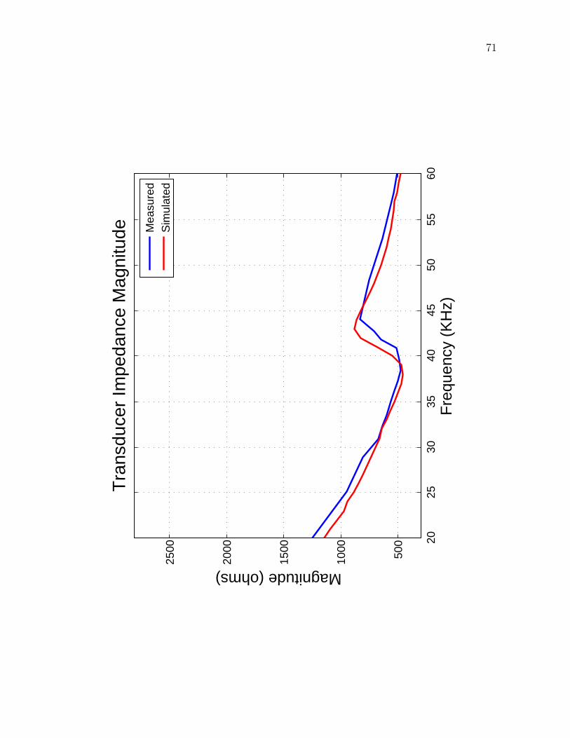
71
2025
3035
4045
5055
60
500
1000
1500
2000
2500
Tra
nsdu
cer
Impe
danc
e M
agni
tude
Fre
quen
cy (
KH
z)
Magnitude (ohms)
M
easu
red
Sim
ulat
ed
Fig
ure
6.14
:M
easu
red
an
dS
imu
late
dIm
ped
an
ce
Magn
itu
de
of
the
Tra
nsd
ucer

72
2025
3035
4045
5055
60
−90
−85
−80
−75
−70
−65
−60
−55
−50
−45
−40
Tra
nsdu
cer
Impe
danc
e P
hase
Fre
quen
cy (
KH
z)
Phase (degrees)
M
easu
red
Sim
ulat
ed
Fig
ure
6.15
:M
easu
red
an
dS
imu
late
dIm
ped
an
ce
Ph
ase
of
the
Tra
nsd
ucer

73
As the transducer is mostly capacitive, the impedance matching circuit
consists of a single 2.5 mH inductor. This inductor value was experimentally
chosen to make the circuit look mostly resitive (0 phase) around the operating
frequency (40 kHz).
R
L
C
CS
DC ZL
ZS
VL
+
-
Baseband
LPF
-90 degree
phase shift
Baseband
LPF
LPFVCOInput
Output
DDC,
Modulator
Synchronizer,
Demodulator
Reference
Symbol clock
192 KHz 16 KHz 4 KHz 800 Hz 200 Hz
Clock Source
Transducer
+ Input
- Input
Figure 6.16: Transducer Impedance Matching Circuit
With the circuit shown in Figure 6.16, Figures 6.17, 6.18, and 6.19 show
the new measured and simulated current, impedance magnitude, and phase of the
transducer when combined with the impedance matching inductor. The figures
still show a relative minimum impedance and relative maximum current around
40kHz. Figure 6.19 shows the circuit is mostly resistive (close to 0 degree phase)
between 35kHz and 45kHz suggesting the circuit could be fairly power efficient in
this range.

74
2025
3035
4045
5055
60051015202530Tra
nsdu
cer
+ 2
.5 m
H In
duct
or C
urre
nt M
agni
tude
Fre
quen
cy (
KH
z)
Magnitude (mA)
M
easu
red
Sim
ulat
ed
Fig
ure
6.17
:Im
ped
an
ce
Matc
hed
Measu
red
an
dS
imu
late
dC
urr
ent
of
the
Tra
nsd
ucer

75
2025
3035
4045
5055
60
500
1000
1500
2000
2500
3000
3500
4000
Tra
nsdu
cer
+ 2
.5 m
H In
duct
or Im
peda
nce
Mag
nitu
de
Fre
quen
cy (
KH
z)
Magnitude (ohms)
M
easu
red
Sim
ulat
ed
Fig
ure
6.18
:Im
ped
an
ce
Matc
hed
Measu
red
an
dS
imu
late
dIm
ped
an
ce
Magn
itu
de
of
the
Tra
nsd
ucer

76
2025
3035
4045
5055
60
−80
−60
−40
−20020406080T
rans
duce
r +
2.5
mH
Indu
ctor
Impe
danc
e P
hase
Fre
quen
cy (
KH
z)
Phase (degrees)
M
easu
red
Sim
ulat
ed
Fig
ure
6.19
:Im
ped
an
ce
Matc
hed
Measu
red
an
dS
imu
late
dIm
ped
an
ce
Ph
ase
of
the
Tra
nsd
ucer

77
Although the power coupled into the transducer cannot directly be mea-
sured, we can use the equivalent circuit in PSpice to estimate the power delivered
to the load. Figure 6.20 shows the majority of the amplifier’s output power is
coupled into the transducer between 35kHz and 45kHz as expected from Figure
6.19.
Figure 6.20: Estimated Power Coupled into the Transducer
6.4 Pre-Amplifier Design
When designing the pre-amplifier for the receiver, we considered the follow-
ing requirements:
• The pre-amplifier must amplify signals around the transducer’s resonance
frequency (40kHz) and filter out all other frequencies
• The pre-amplifier must provide high gain to pick up signals as small as a
couple hundred microVolts
• The design must be easily modifiable to accommodate different transducers
with different resonance frequencies and bandwidths
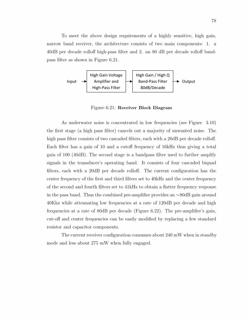
78
To meet the above design requirements of a highly sensitive, high gain,
narrow band receiver, the architecture consists of two main components: 1. a
40dB per decade rolloff high-pass filter and 2. an 80 dB per decade rolloff band-
pass filter as shown in Figure 6.21.
L
C
Transducer
+ Input
- Input
Transmitter
Output +
-
Vout
Receiver Input
Impedance Matching
Network + Input
12:48
12:36
12:24
12:12
Impedance Matching
Network - Input
SW4
SW3
SW2
SW1
SW5
Input OutputHigh Gain / High Q
Band-Pass Filter 80dB/Decade
High Gain Voltage Amplifier and
High-Pass Filter
Figure 6.21: Receiver Block Diagram
As underwater noise is concentrated in low frequencies (see Figure 3.10)
the first stage (a high pass filter) cancels out a majority of unwanted noise. The
high pass filter consists of two cascaded filters, each with a 20dB per decade rolloff.
Each filter has a gain of 10 and a cutoff frequency of 16kHz thus giving a total
gain of 100 (40dB). The second stage is a bandpass filter used to further amplify
signals in the transducer’s operating band. It consists of four cascaded biquad
filters, each with a 20dB per decade rolloff. The current configuration has the
center frequency of the first and third filters set to 40kHz and the center frequency
of the second and fourth filters set to 41kHz to obtain a flatter frequency response
in the pass band. Thus the combined pre-amplifier provides an ∼80dB gain around
40Khz while attenuating low frequencies at a rate of 120dB per decade and high
frequencies at a rate of 80dB per decade (Figure 6.22). The pre-amplifier’s gain,
cut-off and center frequencies can be easily modified by replacing a few standard
resistor and capacitor components.
The current receiver configuration consumes about 240 mW when in standby
mode and less about 275 mW when fully engaged.

79
0
10
20
30
40
50
60
70
80
90
Gain (dB)
Freq
uenc
y (k
Hz)
Rec
eive
r Vol
tage
Gai
n
0
10
20
30
40
50
60
70
80
90
Gain (dB)
Freq
uenc
y (k
Hz)
Rec
eive
r Vol
tage
Gai
n
Fig
ure
6.22
:O
vera
llR
eceiv
er
Gain

80
6.5 Summary
This chapter described the full design of the analog transceiver including the
power amplifier, power management circuit, impedance matching circuit, and pre-
amplifier. The power amplifier is linear in the 10-100kHz band for inputs greater
than 500 mVpp and up to 95% efficient for high power outputs. The impedance
matching circuit makes the transducer look resistive between 35-45kHz coupling
the majority of the amplifier’s output power to the transducer in that frequency
band. The pre-amplifer provides a flat, high gain for frequencies 38-42kHz match-
ing the operating frequency of the transducer and allowing for reception of a signal
as low as 200 microvolts. The power management circuit provides five different
output power levels that consume 1.2, 1.8, 2.7, 4.5, and 6.9 Watts respectively
allowing the modem to adjust the output power in real-time to match it to the
actual distance between transmitter and receiver. All components can be easily
modified by replacing a few standard components.
The next chapter describes the design of the digital transceiver.

Chapter 7
Digital Design
This chapter describes the digital design of the UCSDModem. We begin
with a discussion on different modulation schemes, describing the reason for the
selection of the use of frequency shift keying (FSK). We then discuss various digital
hardware platforms and the selection of a field programmable gate array (FPGA)
for our design. These discussions are followed by a thorough description of the
FPGA implementation of the FSK digital transceiver, including the modulator,
digital down converter, symbol synchronizer, demodulator, clock structure, and
HW/SW Co-design controller. The chapter concludes by presenting the resource
requirements of the complete digital design.
7.1 Modulation Schemes
As described in Chapter 4, various modulation schemes have been imple-
mented in existing commercial and research modems. These schemes all attempt
to combat the performance limitations induced by the underwater acoustic channel
while at the same time improving the bandwidth efficiency and bit rate as much as
possible. This section briefly describes the characteristics of some of these schemes
and reasons for our selection of the use of frequency shift keying for our modem
design.
Frequency Shift Keying: Frequency shift keying is a simple modulation
scheme that has been widely used in underwater communications over the past two
81

82
decades [75, 67]. In M-ary FSK, the data are transmitted by shifting the frequency
of a continuous carrier to one of M discrete frequencies. The simplistic receiver
typically compares the energy at different frequencies to infer what data have been
sent (Figure 7.1). Using only non-coherent energy detection at the receiver, this
scheme bypasses the need for phase tracking which is a very difficult task because
of Doppler spread in the underwater channel. [123] To combat intersymbol inter-
ference caused by multipath and frequency spreading, guard intervals are typically
inserted between successive symbol transmissions for channel clearing [42] or sym-
bols with durations longer than the multipath spread are used. As a result, the
data rate of FSK is very low. Frequency hopped FSK improves the data rate as it
does not need to wait for channel clearing but requires a larger bandwidth. The
minimum theoretical bandwith for a binary FSK scheme is 2X the bit rate (in Hz).
Figure 7.1: Block diagram of classic matched filter FSK demodulator
Phase Shift Keying: In M-ary phase shift keying (PSK), the data are
transmitted by shifting the phase of a continuous carrier to one of M discrete
phases. PSK signals require less transmitted power for a given probability of error
than FSK systems (as shown in Figure 7.2) and require less bandwidth (the mini-
mum theoretical bandwith for a PSK scheme is bit rate (in Hz)) , but require more
coherent detection, either by regenerating a local carrier in the receiver (as shown
in Figure 7.3, or by using differential detection in which the previous bit is used as
the phase reference for the current bit [124]. Although coherent detection could be
used with FSK, the complexity required in the receiver for carrier regeneration jus-
tifies the better bit error rate (BER) performance of PSK. To combat intersymbol
interference caused by multipath and frequency spreading, channel equalization

83
techniques are exploited. Decision feedback equalizers are used to track slowly
varying channels and used to track faster varying channels when combined with a
Phase locked loop [125]. Parameters in the equalizer may have to be fine-tuned to
meet channel conditions. As coherent modulation does not have to wait for chan-
nel clearing, higher bit rates may be achieved at the expense of a more complex
receiver.
0 2 4 6 8 10 12 14 16 1810
−8
10−7
10−6
10−5
10−4
10−3
10−2
10−1
100
Eb/N0 (dB)
BE
R
Coherent−2FSKNonCoherant−2FSK2PSK
Figure 7.2: Bit Error Rate of MFSK and MPSK for a given probability oferror
Direct Sequence Spread Spectrum: In DSSS modulation, the trans-
mitted signal takes up more bandwidth than the information signal that is being
modulated by multiplying each symbol with a spreading code and transmitting
the resulting sequence at a rate allowed by the wider bandwidth. Due to the auto-
correlation properties of the spreading sequence, intersymbol interfere caused by
the underwater channel is suppressed by the de-spreading operation at the receiver.
Channel estimation and tracking are needed if phase-coherent modulation such as

84
Figure 7.3: Block diagram of a coherant PSK receiver
phase-shift-keying (PSK) is used to map information bits to symbols before spread-
ing [126]. For noncoherent DSSS, channel estimation and tracking may be avoided
by using the information bits to select different spreading codes and comparing
the amplitudes of the outputs from different matched filters (each matched to one
spreading code) at the receiver [42]. Direct sequence spread spectrum techniques
such as those seen in [80] require less transmitted power for a given probability of
error than FSK.
Orthogonal Frequency Division Multiplexing: Orthogonal Fre-
quency Division Multiplexing (OFDM) is often referred to as multicarrier mod-
ulation because it transmits signals over overlapping sub-carriers simultaneously.
Sub-carriers (specific frequency bands) that experience higher SNR, are allotted
with a higher number of bits, whereas less bits are allotted to sub-carriers experi-
encing lower SNR. Underwater OFDM has been shown to provide data rates of 12
kbps, 25 kbps, and 50 kbps with bandwidths of 12kHz, 25kHz and 50kHz respec-
tively [95]. The subcarriers are divided in a way to ensure that each carrier is long
compared to the multipath spread in the channel [127, 128] so that intersymbol
interference may be ignored, greatly simplifying the receiver complexity. Although
intersymbol interference may be ignored, the large Doppler spread in the underwa-
ter channel introduces significant interference between subcarriers; thus receivers
must be designed to overcome intercarrier interference increasing their complexity.
Selection of FSK: The proven robustness of FSK and its simplicity make

85
it an attractive modulation scheme for our low-cost modem design for short-range,
low-data rate applications. The scheme requires a simple receiver which can fit onto
a small, low-power device as evidenced by the FSK mode of the WHOI modem
which only uses 0.18 W for the receive processing as compared to its PSK receiver
which uses 2 W for processing [139], or the UCSB DSSS AquaModem which uses
1.6 W for processing [140]. Binary FSK also does not require a large bandwidth
which is suitable for our narrow-band low-cost transducer and corresponding analog
transceiver design. Although data rates are low, they are suitable for the low-data
rate applications of interest.
7.2 Hardware Platforms
This section briefly discusses four possible digital hardware platforms for our
digital transceiver design including Microcontrollers (MCUs), Digital Signal Pro-
cessors (DSPs), Application Specific Processors (ASICs), and Field Programmable
Gate Arrays (FPGAs). We highlight the advantages and disadvantages of each
platform and describe the selection of an FPGA for the UCSDModem.
Microcontrollers: Microcontrollers, or MCUs, are general-purpose de-
vices consisting of a relatively small CPU, clocks, timers, I/O ports and memory.
They are used for information processing and control and can be adapted to a wide
variety of applications by software. Microcontrollers offer design flexibility and non
recurring engineering costs as they can be easily reprogrammed in software and are
widely available. The disadvantage is that an MCU has limited computation abil-
ities and is only a viable solution for relatively simple applications at low sample
rates. Compact code that makes the most efficient use of the MCU architecture is
essential.
A few research underwater acoustic modem designs discussed in Chapter 4
make use of microcontrollers, including the Atmega128L [77, 82] and the Blackfin
533 [83]. The design in [77] is claimed to have a power consumption of only 25mW,
but it relies on an RF ASIC to do most of the processing. The Blackfin 533 used
in [83] is claimed to have a power consumption of 280 mW [129].

86
Digital Signal Processors: Digital signal processors are specialized
microprocessors with an optimized architecture for the fast operational needs of
digital signal processing applications [130]. DSPs offer many architectural features
that reduce the number of instructions necessary for efficient signal processing.
Integrated specialized compute engines increase performance by executing complex
functions in hardware. Like MCUs, DSPs offer design flexibility and non recurring
engineering costs as they can be easily reprogrammed in software and are widely
available. Until recent years, DSPs were notoriously power hungry, but with the
advent of new low-power, fixed point DSPs, power consumption has come down.
Most existing research underwater modem designs (both commercial and
research) make use of DSPs as they are relatively easy to program and can meet the
computational requirements of more complex digital signal processing algorithms.
The DSSS design in [80] and the PSK design in [75] both make use of a floating-
point TI TMS320C6713 processor and consume 2W and 1.6 W respectively. The
FSK mode of [75] makes use of a low-power fixed point DSP consuming only
180mW of power.
Application Specific Processors: An application specific processor,
or ASIC, is custom-designed for a particular application, with as much system
functionality implemented on a single die. ASICs offer exceptional performance,
small size, and low power as they optimize transistor use and clock cycles at the
expensive of flexibility. They have been shown to offer 20X [131] to orders of mag-
nitude lower power consumption than any competing platform [132] . ASICs have
a long time to market and high non recurring engineering costs making them prac-
tical only for high volume production or for designs that demand extremely tight
size and power requirements. To the best of our knowledge, no ASIC underwater
acoustic modem exists.
Field Programmable Gate Arrays: A field programmable gate array
is an integrated circuit designed to be configured by the customer or designer after
manufacturing. FPGAs strike a balance between solely hardware (ASIC) and solely
software (DSP or MCU) solutions as they have the programmability of software
with performance capacity approaching that of a custom hardware implementation.

87
They also present designers with substantially more parallelism allowing for a
more efficient application implementation [133, 134, 135, 136, 137, 138]. Studies
have shown that FPGAs have evolved into highly valued digital signal processing
solutions platforms that reduce overall system costs and power consumption for
high throughput applications [141, 142](further comparison studies are required to
determine whether an FPGA provides power and cost benefits for simpler, lower
throughput applications [142]). However, they require specialized knowledge and
increased design time over DSP and MCUs.
Of the research modems we discussed in Section 2, none solely make use of
an FPGA, although two designs use an FPGA for pre-processing [86, 87]. Power
consumption estimates are not provided.
Selection of FSK: As FSK based underwater acoustic modems have al-
ready been implemented on a DSP [75] and a Microcontroller [83], we selected to
implement our FSK modem on an FPGA to serve as a comparison (particularly
in terms of cost and power consumption) to these designs. Also, FPGAs provide
a relatively easy transition to ASIC should a large volume of modems need to be
produced.
7.3 Digital Transceiver
Now that we have described the selection of the modulation scheme and the
hardware platform, this section provides a thorough description of our FPGA im-
plementation of the FSK digital transceiver, including the modulator, digital down
converter, symbol synchronizer, demodulator, and clock structure. The complete
design is shown in Figure 7.4. Each component was designed in Verilog and ini-
tially tested individually in ModelSim [143] to verify its operation prior to system
integration.

88
sel
sel
Fig
ure
7.4:
Blo
ckD
iagra
mof
Com
ple
teD
igit
al
Receiv
er

89
The digital transceiver design makes use of the parameters given in Table
7.1. The carrier frequency and frequency separation were selected to match the
transducer’s resonance frequency and narrow bandwidth. Nyquist sampling neces-
sitates that the signal be sampled at 2X the frequency of the highest frequency
component of the signal, but in practical applications 4-6X sampling is desired.
Thus the given sampling frequency and processing frequency were selected to pro-
vide sufficient oversampling of the desired frequency component while being integer
multiples of one another. The symbol duration was selected to provide a suitable
raw bit rate for low-data rate sensor networking applications.
Table 7.1: Digital Transceiver Parameters
Properties Assignment
Modulation FSKCarrier Frequency 40 kHzMark Frequency 2 kHzSpace Frequency 1 kHzSymbol Duration 5 msSampling Frequency 192 kHzProcessing Frequency 16 kHz
7.3.1 Modulator
In a digital transceiver, the modulator is responsible for translating a bit
stream into a waveform that can be physically transmitted. For binary FSK,
digital data are transmitted over the analog channel by shifting the frequency
of a continuous carrier to the ‘mark’ or ‘space’ frequency every symbol period
depending on whether a digital ‘1’ or ‘0’ is present respectively. Figure 7.5 shows
the implementation of the FSK modulator. The modulator takes a binary input
(data in) and selects (sel) to generate a sinusoidal wave (Signal out) with the
mark or space frequency using a cosine look-up table (COSLUT ). The correct
frequency is generated by calculating the phase angle offset required to represent
the desired frequency and accumulating the phase offset over one symbol period
to produce the sine wave (Phasecalculation). The offset is calculated using the

90
formula:
Offset = round(size ∗ F/Fs) (7.1)
Where size is the number of elements in the look up table, F is the mark or
space frequency and Fs is the sampling rate (in our case 192kHz). The only area
consuming portion of the modulator is the cosine look up table. To save resources,
we selected a look up table of size 65536 - the smallest look up table that produced
offsets that were different enough to distinguish between the desired mark and
space frequencies.
Figure 7.5: Block Diagram of FSK Modulator
7.3.2 Digital Down Converter
The digital down converter, DDC, (Figure 7.6) is responsible for converting
high resolution signals to lower resolution signals to simplify subsequent process-
ing. It takes the incoming signal from the ADC (adc in) and multiplies it with a
continuous 40kHz signal generated from a cosine look up table (COSLUT ) using
the same phase calculation (Phasecalculation) method described in the previous
section. The mixed signal then passes through a 5kHz low pass filter (LPF5K)
to filter out the high frequency components of the mixed signal leaving a 1k signal
as the space frequency and a 2kHz as the mark frequency (Signal out). The DDC
then down samples the signal from 192kHz to 16kHz, the processing frequency.
To reduce the resource usage of the down converter, the look up table from the

91
modulator is reused (as the modem cannot transmit and receive at the same time).
The low-pass filter is a small 20-tap FIR filter designed using Spiral [144], a filter
design program from Carnegie Mellon well known for creating compact filters.
Figure 7.6: Block Diagram of Digital Down Converter
7.3.3 Symbol Synchronizer
Symbol synchronization, the ability of the receiver to synchronize to the
first symbol of an incoming data stream [145], is a critical component in the design
of an underwater acoustic modem. When the modem receiver obtains an input
stream, it must be able to find the start of the data sequence to set accurate
sampling and decision timing for subsequent demodulation. Symbol synchroniza-
tion is particularly important in the underwater acoustic channel as the channel
can be highly variable and plagued by multipath, variable noise levels, path-loss,
Doppler shifts, and long propagation delays [146, 19]. Without accurate symbol
synchronization, higher bit error rates incur thus reducing the reliability and qual-
ity of service of the wireless network. As the symbol synchronizer is the most
complicated aspect of the digital transceiver design, many pages are devoted to its
description. We describe the selection of symbol syncrhonization scheme and its
hardware implementation.

92
Synchronization Scheme
The most common and simple symbol synchronization approach relies on
the transmission of a predefined sequence of symbols, often referred to as a train-
ing, or reference sequence. The transmitter sends a packet that begins with the
reference sequence and the receiver compares the received sequence with the known
reference sequence in order to locate the start of the packet [145, 147]. The com-
parison is effectively performed by correlating the received sequence with the ref-
erence sequence when a new sample is received. When the reference and receiving
sequence exactly align with each other, the correlation result reaches a maximum
value and the synchronization point is located (Figure 7.7).
Figure 7.7: Process of Symbol Synchronization
Though this synchronization method is straight forward in theory, there are
many design choices that must be considered before implementing the algorithm:
• How can the peak correlation result be detected effectively?
• What reference code is appropriate for the application?
• How will the reference code be represented?
• How long should the reference code be?
Typical methods to detect a correlation peak involve setting a correlation
threshold where the correlation result only rises above the threshold when the

93
receiving sequence and reference sequence are perfectly aligned. The threshold
must be large enough to minimize the number of false alarms (the system detects
the reference code is present when it is not), but small enough to guarantee the
peak will still be detected when the signal level is low.
The underwater acoustic channel is highly variable and plagued by variable
noise levels, path-loss, and long propagation delays [146, 19]. Thus, selecting
a static correlation threshold for the underwater receiver is impractical as the
received signal strength and noise level are changing in real-time. We therefore
need to set a dynamic correlation threshold based on a dynamic estimation of
the noise level. As a data packet could be sent at any time, it is hard to find a
suitable rate for the receiver to take ‘noise’ samples periodically to set the dynamic
threshold. The receiver must be able to set an appropriate threshold whether data
or noise are present. The goal can be achieved through the use of an orthogonal
reference sequence. As shown in equations (7.2-7.5), the receive sequence, R(t),
contains both the delayed transmitted sequence (the reference sequence followed
by data), S(t−τ), and noise n(t) in (7.2). When we correlate the received sequence
with the reference code, r(t), and the orthogonal reference code ro(t) at the receiver
separately, the correlation result of the reference branch C(t) (7.3) contains both
signal and noise portions, whereas the correlation result of the orthogonal branch
Co(t) (7.4) contains solely the noise correlation result. We can therefore estimate
the real-time noise level by calculating the standard deviation of the correlation
result of the orthogonal branch T (t) (7.5) and set the threshold according to this
result. Though the threshold calculation is not a true estimate of the noise (as it
includes the ‘noise’ from the imperfection of the orthogonal correlation), it serves
as a reasonable threshold for peak detection.

94
R(t) = S(T − τ) + n(t) (7.2)
C(t) = R(t) ∗ r(t) = ΣjR(t)r(t+ j) (7.3)
Co(t) = R(t) ∗ ro(t) = ΣjR(t)ro(t+ j)
= ΣjS(t− τ)ro(t+ j) + Σjn(t)ro(t+ j)
= Σjn(t)ro(t+ j) (7.4)
T (t) = ΣjCo(t)2 = Σjn(t)2ro(t+ j)2 (7.5)
In order to make use of the scheme described above, we must select a ref-
erence code that has an excellent periodic and aperiodic autocorrelation function,
and an excellent cross-correlation function (with values close to zero) with its or-
thogonal code. We considered using Gold codes, Walsh codes, and PN sequences.
Figure 7.8 shows the autocorrelation (blue) and cross-correlation with an orthog-
onal code for the Gold, Walsh, and PN sequences respectively.

95
(a)
(b)
(c)
Figure 7.8: Auto Correlation (blue) and Cross Correlation (black) of Orthog-onal Gold (a), Walsh (b) and PN (c) Reference Codes

96
Because of the Gold Code’s superior autocorrelation and cross correlation
properties, we selected to use two orthogonal Gold Codes for our reference and
orthogonal reference sequence. Gold codes show reasonable cross-correlation and
off-peak autocorrelation values while providing perfect orthogonality in the zero-
offset case [147].
Gold codes are binary sequences of length 2m-1 consisting of ‘1’s and ‘-1’s.
As the underwater acoustic receiver uses FSK modulation, we can represent the
Gold code by using the mark frequency to represent a ‘1’ and a space frequency to
represent a ‘-1.’ However, representing the Gold code as a sequence of sinusoids
eclipses its desired auto-correlation and cross-correlation properties. Thus we need
to introduce a ‘signal shaping’ function before computing a correlation to make
the receiving sequence look like a sequence of ‘1s’ and ‘-1s’ instead of a sequence
of sinusoids.
We select an appropriate reference length for the Gold code by simulating
the symbol synchronization method in MATLAB with a packet consisting of Gold
code of lengths 3, 7, 15, and 31 followed by 80 symbols of data with a value of 15dB
SNR. Ten thousand simulations produced correct results and a sharp and distinct
peak for the synchronization point for packets with Gold codes of length 15 and
31, but failed to produce accurate results for packets with Gold codes of length 7
and 3. Thus, we select a reference code length of 15 as it is the minimum length
that provides accuracy. Figure 7.9 shows the simulation result for a packet with
a reference code of length 15. The dashed line shows the result of the orthogonal
correlation, the thick line shows the resulting threshold and the solid line shows
the reference correlation result. The result of the correlation and orthogonal corre-
lation is virtually zero when only noise is present. The correlation result first rises
above the threshold when the data packet is present and the synchronization point
is accurately detected as the highest point above the threshold within the follow-
ing two reference lengths. A two reference length period is selected as the peak
searching interval because it takes two reference lengths for an incoming reference
signal to enter and exit the interval of correlation.

97
020
040
060
080
010
0012
00-2-10123
sam
ples
corre
lated
sign
alco
rrelat
ed o
rthog
onal
signa
lad
aptiv
e thr
esho
ld
Fig
ure
7.9:
MA
TL
AB
sim
ula
tion
of
sym
bol
syn
chro
niz
ati
on
for
un
derw
ate
rF
SK

98
Our symbol synchronization scheme for underwater FSK is therefore given
in Figure 7.10. The input signal, Sig in, is the baseband signal coming from the
DDC. The signal first passes through a signal shaping block which shapes the input
signal from a sinusoid to a square-like wave. The signal shaping block consists of
the same mark and space filters as those in the demodulator followed by a down
sampler, absolute value operation, and subtraction. The effect of the filters is
to remove out-of-band noise and begin to shape the signal as having regions of
different amplitudes. The down sampler and absolute value operations further
smooth the signal into an all positive square-like wave. The subtraction produces
the desired square-like wave consisting of positive and negative numbers ready for
correlation with the reference code consisting of ‘1s’ and ‘-1s.’
After the signal passes through the shaping block, it then performs a par-
allel correlation with the expected reference code and orthogonal reference code.
The result of the correlation with the orthogonal branch is squared and summed to
compute its standard deviation and serve as a threshold for the reference code cor-
relation operation (as previously described). The ‘find max index’ logic compares
the reference correlation result with the threshold. When the reference correlation
result rises above the threshold, the logic looks for the highest peak above the
threshold over two reference length periods to ensure it can find the highest peak
that denotes the synchronization point. The index of peak position is recorded
and sent to the demodulator for accurate symbol timing.
Figure 7.10: Block Diagram of Symbol Synchronization for Underwater FSK

99
Hardware Implementation
In order to implement our symbol synchronization design into hardware,
we need to consider the design parameters of our acoustic receiver. Recall that the
ADC sampling rate is 192KHz and the symbol period is 5ms. These parameters
give a total of 960 samples per symbol. With a reference length of 15 symbols,
the entire reference sequence is 14,400 samples. Multiply that by 2 to include the
orthogonal reference sequence. Correlating 28,800 samples requires 28,800 multi-
plications and 28,798 additions. These operations are either too area-consuming
or computationally infeasible to complete in one 192KHz sampling clock period
(5.2 us). We thus focus our hardware design implementation on reducing the
complexity of the correlation.
The signal shaping block down samples the incoming signal to shape the
signal into a square-like wave. As a square wave only requires one bit to repre-
sent the sequence, we down sample the original signal by 240 to create a signal
sequence consisting of 4 samples per symbol (4x oversampling), or 60 samples. We
therefore require a correlater that can handle 120 multiplications (including the
orthogonal branch) and 118 additions in one 800Hz (192kHz/240) clock period.
Our correlation architecture (for one correlation branch) is given in Figure 7.11.
In each 800Hz clock period, the shaped signal is shifted into a 60 element shift
register that must be correlated with the reference signal. In order to reduce the
path length, we applied a 4KHz local clock to pipeline the storing. As the reference
signal is represented by ‘1’s and ‘-1’s, we can simplify the correlation operation by
replacing the multiplications with a sign selection method (SS core): when the
reference signal is a ‘1’, add the relevant stored shaped signal, when the reference
signal is a ‘-1’ subtract the relevant stored shaped signal.

100
… …
Sh
ift re
gis
ter
se
qu
en
ce
sh
ap
ed
sig
na
l1
60
... ...
...
...
...
12
15
14
16
30
16
...
...
31
45
46
47
59
60
M U
XM
U X
M U
XM
U X
co
un
ter
S S
core
S S
core
S S
core
S S
core
Re
fere
nce
sig
na
l
Re
fere
nce
sig
na
l
Re
fere
nce
sig
na
l
Re
fere
nce
sig
na
l
+C
orr
ela
tio
n r
esu
lt
80
0H
z
4K
Hz
16
KH
z
80
0H
z
Clo
ck r
eg
ion
45
Fig
ure
7.11
:H
ard
ware
Un
its
of
Corr
ela
tion
Imp
lem
enta
tion
for
Un
derw
ate
rF
SK

101
We implement the correlation in a 15-stage pipeline,as a fully parallel shift
register implementation would require too many resources and a fully serial shift
register implementation would require a significantly faster clock. The appropriate
15 elements of the shift register are serially selected into an SS core at a 16KHz
clock rate to achieve a partial correlation result. The outputs of four SS cores
are then summed in one 800Hz clock period to produce the complete correlation
result. Thus we achieve a compact, timing accurate correlation implementation.
The symbol synchronization has a delay of eighty 16KHz clock cycles, one for
clocking data in, 60 for shifting the signal into the correlator, 15 for the pipelined
additions and 4 for shifting the result to the output.
The rest of the symbol synchronization design is computationally inexpen-
sive; the filters consist of two small 20-tap FIR filters designed using [144] and the
threshold calculator only requires one multiplier and one adder. The 800Hz clock
used for synchronization is source synchronous with the 192KHz sampling clock
and 16KHz demodulator clock to avoid clock confliction.
Upon startup the modem must initialize the known reference code and
orthogonal reference code to memory at the 192KHz clock rate and perform an
initial correlation over one reference length (60, 800Hz clock cycles) to ensure a
valid threshold value. The total initialization occupies 75ms.
After initialization, the synchronizer executes as previously described: shap-
ing the incoming signal, correlating it with the reference code and orthogonal ref-
erence code and searching for a correlation result above the threshold. When the
reference correlation result rises above the threshold, the block looks for the high-
est peak above the threshold over two reference length periods to ensure it can find
the highest peak that denotes the synchronization point. The control structure is
shown in Figure 7.12 and described in the following paragraphs.

102
Fig
ure
7.12
:C
ontr
ol
Str
uctu
reof
Sym
bol
Syn
chro
niz
ati
on
for
Un
derw
ate
rF
SK

103
When the correlation result first rises above the threshold, we assume that
this point is the synchronization point and thus need to start the symbol clock.
Recall that the down-sampled clock used for synchronization is 800Hz and the
symbol clock is 200Hz; therefore a symbol clock can be formed by 4 cycles of the
down-sampled clock. Thus, at the time a peak occurs (1st peak), a reset signal is
asserted (Rst symbol cnt) to reset a 2 bit counter (Symbol clk cnt) which is used
to generate the symbol clock every four 800Hz cycles. In the meantime, the index
of the peak location, A, is stored into a real-time index register (index reg) and
the demodulator is enabled (en dem). The real-time demodulated values are then
stored in a temporary buffer and the number of demodulated symbols is counted
by another counter (symbol num count).
If another, larger peak, occurs within two reference lengths (2nd peak),
rst symbol cnt is asserted to resynchronize the symbol clock at this higher peak
point. The value of index reg is also replaced to B (the number of samples offset
from the initial peak A). The counter, symbol num count, continues to count
the number of demodulated symbols and the demodulated results are stored in
a temporary buffer. The values already demodulated between A and B will be
ignored as the peak at A was not the maximum. When an even larger, real peak
occurs (3rd), rst symbol cnt is again re-asserted to resynchronize the symbol clock
at this higher peak. The value of index reg is set to C (the number of samples
offset from the initial peak A). Since B was not the maximum either, the values
already demodulated between time A and C will have to be ignored.
At the end of two reference lengths, the location of the maximum peak, C,
can be found in index reg and the number of symbols demodulated since the first
peak can be found in symbol num count. We can then calculate the address of
the first valid piece of data in the temporary buffer with the following equation:
addr = symbol num cnt− round[NO OF SAMPLES − 1− index reg
DS FACTOR
](7.6)
where NO OF SAMPLES is the number of samples in two reference
lengths (120), DS FACTOR is the down sampling factor between the synchroniza-
tion clock (800Hz) and the symbol clock (200Hz) and round[(NO OF SAMPLES−

104
1−index reg)/DS FACTOR] gives the number of symbols demodulated since the
synchronization point (C) found in index reg.
After the modem has demodulated the entire packet, it desserts the en dem
signal and the synchronizer returns to searching for a correlation result above the
threshold to synchronize on the next incoming packet.
Figure 7.13: Block Diagram of Matched Filter FSK Demodulator
7.3.4 Demodulator
A demodulator converts the analog waveform it receives back into the digi-
tal signal that was transmitted. For FSK, this means it detects the mark and space
frequencies in the received signal and converts them back to digital ‘1’s and ‘0’s
respectively. The classic ‘matched’ filter demodulator is optimal for FSK detec-
tion with white Gaussian noise interference [148]. The demodulator (Figure 7.13)
works by sending a symbol duration of the received signal (the output of the DDC)
through two bandpass filters (one filter that is centered around the mark frequency
(2kHz) and the other that is centered around the space frequency (1kHz)). The
demodulator then integrates the output of each filter over one symbol period (en-
ergy detection) to determine the relative amount of energy in each frequency band.
If the energy of the mark filter is greater than the energy of the space filter a ‘1’
was sent whereas if the energy of the space filter is greater than the energy of the
mark filter a ‘0’ was sent. Our matched filter demodulator uses the same compact
filters as the symbol synchronizer designed by [144]. To save design space, no em-
bedded multiplier is used in our demodulator. The decision module includes two

105
accumulators in order to add the output of low pass filters in a symbol period, and
a comparator to select the greater one of the accumulators to make the decision.
7.3.5 Clock Generation
The digital transceiver makes use of multiple clocks: the sampling clock,
the baseband clock, the symbol clock, and the clocks used for synchronization.
All clocks are integer divided with logic from a single clock source as shown in
Figure 7.14(a) to avoid clock confliction and ensure they are source synchronous.
An extra flip flop was added between clock domains (as shown in figure 7.14(b))
to avoid random problems caused by metastability.
DDC,
Modulator
Synchronizer,
Demodulator
Reference
Symbol clock
192 KHz 16 KHz 4 KHz 800 Hz 200 Hz
Clock Source
(a)
DDC,
Modulator
Synchronizer,
Demodulator
Reference
Symbol clock
192 KHz 16 KHz 4 KHz 800 Hz 200 Hz
Clock Source
(b)
Figure 7.14: (a) Clock Division, (b) Added Flip Flop between clock domainto avoid metastability

106
7.3.6 HW/SW Co-Design Controller
We used Xilinx Platform Studio 10.1 to build a HW/SW co-design for accu-
rate control and I/O of the digital transciever. The co-design consists of the digital
transceiver, a UART (Universal Asynchronous Receiver Transmitter) to connect
to serial sensors or to a computer serial port for debugging, an interrupt controller
to process interrupts received by the UART or the modem, logic to configure the
on board ADC, DAC, and clock generator, and MicroBlaze, an embedded micro-
processor to control the system (Figure 7.15).
The MicroBlaze processor is a 32-bit Harvard Reduced Instruction Set Com-
puter (RISC) architecture optimized for implementation in Xilinx FPGAs. It inter-
faces to the digital modem through two fast simplex links (FSLs), point-to-point,
uni-directional asynchronous FIFOs that can perform fast communication between
any two design elements on the FPGA that implement the FSL interface. The Mi-
croBlaze interfaces to the interrupt controller and UART core over a peripheral
local bus (PLB), based on the IBM standard 64-bit PLB architecture specification.
modem
MicroBlaze
Interrupt
controllerUART
clocks
ADC
DAC
FPGA
PLB
PLB PLB
FSLFSL
FSL FSL
Figure 7.15: HW/SW Co-Design for the digital transceiver

107
Upon start-up, the MicroBlaze initializes communication with the digital
transceiver through sending a command signal through the FSL bus signaling the
digital transceiver to turn on. When the digital transceiver is ready to begin re-
ceiving signals, it sends an interrupt back to MicroBlaze to indicate initialization
is complete. The digital transceiver then begins the down conversion and synchro-
nization process, processing the signal received from the ADC and looking for a
peak above the threshold to indicate a packet has been received. If the digital
transceiver finds a peak above the threshold, it finds the synchronization point,
and demodulates the packet. The demodulated bits are stored in the FSL FIFO.
modem
MicroBlaze
Interrupt
controllerUART
clocks
ADC
DAC
FPGA
PLB
PLB PLB
FSLFSL
FSL FSL
Figure 7.16: Digital Transceiver Control Flow. Interrupts are shown in red
When the full packet has been demodulated, the digital transceiver sends
an interrupt indicating a packet has been received and the MicroBlaze may retrieve
the packet from the FSL. The digital transceiver then returns to synchronization,
searching for the next incoming packet. After initialization, the MicroBlaze re-
mains idle, waiting for interrupts either from the digital transceiver or UART. If it
receives an interrupt from the digital transceiver indicating that a packet has been
demodulated, the MicroBlaze reads the bits from the FSL FIFO and sends the
bits over the UART to be printed on a computer’s Hyperterminal for verification.
If the MicroBlaze receives an interrupt from the UART, indicating that the user

108
would like to send data, the MicroBlaze sends a command to the transceiver to
send the bitstream the MicroBlaze places in the FSL. The digital transceiver then
modulates the data from the FSL and sends the modulated waveform to the DAC
for transmission. The MicroBlaze then returns to waiting for interrupts from the
transceiver or the UART and the transceiver returns to synchronization, searching
for the next incoming packet. This control flow is depicted in Figure 7.16.
7.4 Resource Requirements
Table 7.2 shows the FPGA hardware resources occupied for each component
of the digital transceiver. The resources reported for ‘Total’ include the complete
digital transceiver and HW/SW co-design controller. These resources were mapped
for a Spartan 3 XC3S4000, the smallest device in the established Spartan 3 family
that can fit the design.
Table 7.2: Digital Design Resource Usage
Occupied Slices LUTs BRAMs
Modulator 95 184 9DDC 284 541 9Demodulator 1025 1980 1Synchronizer 12000 22101 2Total 16706 29076 55(% Spartan3) (60%) (51%) (57%)
We obtained a power estimate of the complete FSK modem design on var-
ious FPGA devices by entering the resource values of the total modem into the
Xilinx XPower Estimator 9.1.03 and the Altera Cyclone IV PowerPlay Early Power
Estimator. We acknowledge that the resource values determined for one device are
not an exact estimate of the resource values needed for another device, but they
do provide us with a reasonable first order resource (and power) estimate. Also
note that the estimates reported for the Xilinx devices are more accurate than
those reported for the Altera device as the current design makes use of a Xilinx
MicroBlaze core which would have to be replaced with the Altera NIOS processor
should the design be implemented on an Altera chip. The devices reported are

109
in device families known for their low power consumption (the Xilinx Spartan 6
and the Altera Cyclone IV being some of the newest FPGA device families on the
market). The particular devices reported are the smallest devices in their family
that fit the total modem design. The letters ‘Q’, ‘D’, and ‘T’ in Table III stand
for ‘quiescent,’‘dynamic’, and ‘total’ power respectively. The last column of Table
7.3 reports the size of device family’s CMOS technology.
Table 7.3: FPGA Power Consumption
Family Device Q Pwr D Pwr T Pwr Tech(W) (W) (W) (nm)
Spartan 3 XC3S4000 0.274 0.105 0.379 90Spartan 6 XC6SLX150T 0.212 0.021 0.255 45Cyclone IV EP4CE30 0.087 0.06 0.147 60
From Table 7.3 we observe that the quiescent power contributes significantly
to the total power of the design. Thus, it is important to select a device that
offers low quiescent power. Altera has invtested considerable resources in reducing
static power in their products as evidenced by our design’s low quiescent power
on the Cyclone IV. Furthermore, the newer technologies (Spartan 6 and Cyclone
IV) consume less power than the older technology, suggesting that with continued
technological advancements, FPGA power consumption will continue to decrease.
Table 7.4 compares the total digital hardware platform processing power
and cost of the UCSDModem design with existing research underwater modem
digital designs that report their total processing power. As previously described,
these research modem designs use various modulation schemes (FSK, PSK, or
DSSS) and are implemented on various hardware platforms.
Table 7.4: Digital Transceiver Design Comparison
Modem Mod Category Platform Total Pwr (W) Cost ($)[139] FSK FixedDSP TMS320C5416 0.180 45[139] PSK FP DSP TMS320C6713 2.0 25[140] DSSS FP DSP TMS320C6713 1.6 25[83] FSK MCU Blackfin 533 0.280 25UCSD FSK FPGA XC6SLX150T 0.233 14Modem EP4CE30 0.147 40
110
From Table 7.4 we notice that the designs implemented on floating point
DSPs consume considerably larger power than any of the other designs. How-
ever, these designs use more complex modulation schemes and thus require more
resources. The FSK design in [139] on the fixed point DSP and the FSK design
in [83] on a microcontroller provide comparable power consumption to our FSK
design on an FPGA.
The cost reported for the DSP, Microcontroller, and FPGA devices were all
found on electronic distributer websites. These estimates suggest that the FPGA
design also provides a comparable cost to other digital hardware platforms.
7.5 Summary
This chapter described the design of the UCSDModem’s FSK FPGA based
digital transceiver including the modulator, digital down converter, symbol syn-
chronizer, demodulator, clock generator, and HW/SW co-design. The design op-
erates at 200 bps in a narrow band around a 40kHz carrier (to match the operating
frequency of the transducer and the design of the analog transceiver) and provides
comparable cost and power consumption to other frequency shift keying based
modem designs. The next chapter describes the system tests used to evaluate the
functionality and performance of the complete modem design.
The text of Chapter 7.3.3 is in part a reprint of the material as it appears in
the proceedings of the IEEE International Conference on Sensor Networks, Ubiq-
uitous, and Trustworthy Computing. The dissertation author was a co-primary
researcher and author (with Ying Li). The other co-authors listed on this publi-
cation [3] directed and supervised the research which forms the basis for Chapter
7.3.3.
The text of Chapter 7.3.1, 7.3.2, 7.3.4, and 7.3.6 is currently being prepared
for submission for publication of the material. The dissertation author is a co-
primary researcher and author (with Ying Li). Ryan Kastner and Xing Zhang
directed and supervised the research which forms the basis for Chapter 7.3.1, 7.3.2,
7.3.4, and 7.3.6.

Chapter 8
System Tests
In order to verify the operation of the UCSDModem, we first tested the
analog components and digital components separately and then tested the full,
integrated system in three different underwater environments at various ranges.
This chapter describes the results of each test and summarizes the performance of
our modem.
8.1 Analog Testing
To test the operation of our analog components (the transducer and analog
transceiver), we took our analog hardware to Mission Bay, a salt water bay near San
Diego, CA. One analog transceiver and transducer was placed on the dock to act
as the transmitter (Figure 8.1 (a)) and another analog transceiver and transducer
was placed on a boat to act as the receiver (Figure 8.1 (b)). The transmitter
was powered by power supplies on the dock and the receiver was powered by a
power supply connected to an inexpensive RadioShack AC/DC converter connected
to the boat’s power that unfortunately produced a substantial amount of noise
(200mVpp).
We sent a 40kHz sinusoid from the transmitter to the receiver placed at
three different locations as shown in Figure 8.2: 1. 75 meters, 2. 235 meters, and
3. 350 meters away. We were able to successfully detect the signal at 350m at the
fourth output power level, however the receive signal was just above 200mVpp at
111

112
(a)
(b)
Figure 8.1:
Mission Bay Test Set Up. (a) Transmitter on dock, (b) Receiver on
boat
this distance and hence could just be detected above the converter’s noise. This
test proved that our analog hardware could transmit a considerable distance and
would likely be able to transmit a farther distance given a low-noise power supply
at the receiver and further improvements to the analog transceiver.

113
Figure 8.2: Mission Bay Receive Distances 1. 75 m 2. 235 m 3. 350 m

114
8.2 Digital Testing
For digital testing, we purchased a prototype test platform, the DINI DMEG-
AD/DA [151] that includes analog-to-digital and digital-to-analog converters, a
Xilinx Virtex-4 FPGA, an onboard oscillator, and a serial port and downloaded
the HW/SW co-design to the board (Figure 8.3). We also purchased two M-Audio
ProFire 610 devices [152] to collect and store received waveforms for post-analysis.
We conducted hard wired and bucket tests of the digital transceiver as described
in the subsections below.
Figure 8.3: DINI DMEG-AD/DA Test Platform
8.2.1 Hard Wired Tests
To verify the functionality of our complete FPGA digital transceiver, we
downloaded the HW/SW co-design to the DINI board, connected the output of
the DAC directly to the input of the ADC, and sent packets consisting of the 15
bit Gold Code of ‘011001010111101’ followed by 8 bits (for easy visual verification
of the data) or 100 bits (a data length comparable to that sent by sensors) of
randomized ones and zeros. We used Hyperterminal to give the command to send
a packet at random times and to display the decoded results of the modem. We
used ChipScope Pro [153] to view the internal waveforms.
Figure 8.4 shows the HyperTerminal window of a test showing the correct
transmission of two 8-bit data packets sent at different times according to the time
the operator pressed the ‘s’ key. The modem continues to rest in a state waiting
to receive the next packet.

115
Fig
ure
8.4:
Hyp
erT
erm
inal
Ou
tpu
tW
ind
ow
show
ing
corr
ect
tran
smis
sion
of
two
hard
wir
ed
pack
ets

116
Figure 8.5 shows some of the internal waveforms and signals from a 100-
bit data length test. The blue signal shows the output of the bandpass filter
centered around the space frequency in the demodulator and the green signal
shows the output of the bandpass fitler centered around the mark frequency in the
demodulator. Notice that the data in signal exactly aligns with the waveforms.
The decoded result (decode result)is a delayed version of the input signal due to
the 80, 16kHz clock cycles required for synchronization initialization.
Fifty 100-bit data length packets were sent, all achieving perfect synchro-
nization and 0% bit error rate thus verifying the correct operation of the hardware.

117
Fig
ure
8.5:
Ch
ipS
cop
eIn
tern
al
Wavefo
rms
an
dsi
gn
als
from
a100-b
itd
ata
len
gth
test
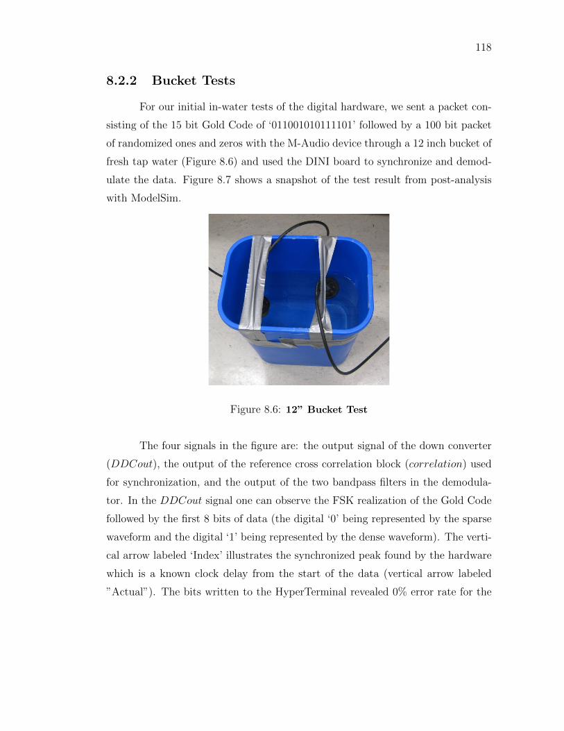
118
8.2.2 Bucket Tests
For our initial in-water tests of the digital hardware, we sent a packet con-
sisting of the 15 bit Gold Code of ‘011001010111101’ followed by a 100 bit packet
of randomized ones and zeros with the M-Audio device through a 12 inch bucket of
fresh tap water (Figure 8.6) and used the DINI board to synchronize and demod-
ulate the data. Figure 8.7 shows a snapshot of the test result from post-analysis
with ModelSim.
Figure 8.6: 12” Bucket Test
The four signals in the figure are: the output signal of the down converter
(DDCout), the output of the reference cross correlation block (correlation) used
for synchronization, and the output of the two bandpass filters in the demodula-
tor. In the DDCout signal one can observe the FSK realization of the Gold Code
followed by the first 8 bits of data (the digital ‘0’ being represented by the sparse
waveform and the digital ‘1’ being represented by the dense waveform). The verti-
cal arrow labeled ‘Index’ illustrates the synchronized peak found by the hardware
which is a known clock delay from the start of the data (vertical arrow labeled
”Actual”). The bits written to the HyperTerminal revealed 0% error rate for the

119
100 bit packet from the 12 inch plastic bucket. Calculating the SNR as:
SNR = 10 ∗ log10
(var(signal)
var(noise)
)(8.1)
at the input to the digital down converter, the SNR in the bucket was 33
dB. The test was repeated with different data bits 10 times all producing 0% error.
Figure 8.7: Snapshot of hardware simulation result for 12” bucket test

120
8.3 Integrated Tests
After verifying the correct operation of the analog and digital hardware
seperately, we conducted integrated system tests of the complete modem design
in a tank, pool, and lake. To protect the digital electronics, we added a voltage
limiter to the output of the pre-amplifier to clip all signals above 1.3Vpp. To
characterize the multipath in the different environments, we sent a 200 ms 35k-
45kHz chirp signal from the transmitter to receiver to measure the multipath delay
spread. The multipath measurements and test results are described in the following
subsections.
8.3.1 Multipath Measurements
As described in Chapter 3, underwater, there exist multiple paths from the
transmitter to receiver, or multipath. Two fundamental mechanisms of multipath
formation are reflection at the boundaries (bottom, surface, and any objects in
the water), and ray bending (where rays of sound bend towards regions of lower
propogation speed). The amount of multipath seen at the receiver depends on the
locations of the transmitter and receiver and the geometric and physical properties
of the environment.
The extent of the multipath at a receiver can be characterized by the mul-
tipath delay spread. Delay spread can be interpreted as the difference between the
time of arrival of the first significant path (typically the line of site component)
and the time of arrival of the last multipath component. Given the amplitude
delay profile, Ac(τ), with effective signal length, M , the mean delay, τ , and the
rms delay spread, τrms, are given as [154] :
τ =
∑Mn=1 τAc(τ)2∑Mn=1Ac(τ)2
(8.2)
τrms =
√∑Mn=1(τ − τ)2Ac(τ)2∑M
n=1Ac(τ)2(8.3)
For frequency shift keying, multipath will cause intersymbol interference
when the multipath delay spread is larger than the symbol duration. Intersymbol

121
interference is a form of distortion of a signal in which one symbol interferes with
subsequent symbols. This is an unwanted phenomenon as the previous symbols
have similar effect as noise, thus making the communication less reliable [155].
Therefore, because the UCSDModem has a symbol duration of 5ms, the delay
spread of the channel must be less than 5ms to ensure reliable communication.
To measure the multipath delay spread of the different test environments,
we sent a 200 ms 35k-40kHz chirp signal from the transmitter to receiver and used
the DAQ device to collect 5 seconds of the received signal containing the chirp. We
then post-processed the received signal, correlating the transmitted waveform (the
2ms chirp) with the received waveform to form the amplitude delay profile. We
then used equations 8.3 and 8.2 to compute the rms delay spread. The amplitude
delay profiles and rms delay spread of each test environment are given in the
following subsections along with performance results.
8.3.2 Tank Tests
We conducted an initial full integrated system test in a 0.5x1x0.5 meter
tank filled with fresh water with the transducers spaced 50 cm apart. Five packets
consisting of the reference code followed by 1000 randomized bits were sent from
transmitter to receiver using all power levels. Calculating the SNR as:
SNR = 10 ∗ log10
(var(signal)
var(noise)
)(8.4)
at the input to the digital transceiver was 28dB for all power levels as the
signal was clipped to 1.3Vpp at each level. All tests revealed 0% bit error rate.
The rms delay spread in the tank was computed to be 1.86 ms from the amplitude
delay profile given in Figure 8.8

122
0 2 4 6 8 10 12−1
−0.8
−0.6
−0.4
−0.2
0
0.2
0.4
0.6
0.8
1
Time (ms)
Am
plitu
de
Tank 0.5m Multipath
Figure 8.8: Multipath Amplitude Delay Profile at 0.5 m in the tank

123
8.3.3 Canyon View Pool Tests
We conducted another full integrated system test at the UCSD Canyon
View Pool, a 50m x 25m concrete pool with 1m depth on the shallow end and 5m
depth on the deep end filled with chlorinated fresh water. At 50 meters distance,
we sent a packet of 400 symbols followed by a 400 symbol clearing period followed
by another packet of 400 symbols using all power levels. The transducers were
submerged to a depth of 10 cm and placed along the 50m side of the pool to avoid
swimmers. The digital hardware was able to successfully detect the start of each
packet, but failed to accurately demodulate the data, achieving only 25% bit error
rate with an SNR of 14dB (for all power levels). The rms delay spread in the pool
was computed to be 21.3 ms from the amplitude delay profile given in figure 8.9,
thus causing severe intersymbol interference. Concrete pools are one of the most
difficult underwater channels due to extremely strong multipath. As expected,
a longer symbol duration or a channel equalizer would have to be added to the
modem to improve the performance of the modem in high multipath environments.
0 10 20 30 40 50 60 70 80 90−1
−0.8
−0.6
−0.4
−0.2
0
0.2
0.4
0.6
0.8
1
Time (ms)
Am
plitu
de
Canyon View Pool 50m Multipath
Figure 8.9: Multipath Amplitude Delay Profile at 50m in the Canyon ViewPool

124
8.3.4 Westlake Tests
After completing tests in a tank and a pool, we conducted full integrated
system tests in Westlake, a freshwater lake in Westlake Village, CA, at 5m, 50m,
95m, and 380m distances as shown in Figure 8.10. The transmitter was located
on a dock, and the receiver was located on a boat. Five packets consisting of
the reference code followed by 1000 randomized bits were sent from transmitter
to receiver using all power levels. Tests at the 95 meter distance and 380 meter
distance were incomplete due to the inability to remain near a private dock for a
length of time.
The multipath amplitude delay profiles for the 5m, 50m, and 95m distances
are given in Figures 8.11, 8.12, and 8.13 with calculated rms delay spreads of
2ms, 1.5 ms, and 2.66 ms respectively. Multipath at the 380 m distance was not
measured.
The SNR at the input to the digital transceiver was 34dB for all power
levels at the 5 meter distance, 21 dB for all power levels at the 50 meter distance,
and 9 dB for power level 4 at the 380 meter distance (power levels 0-3 could not
reach 380 meters). Bit error rates averaged 2.95%, 0.20%, and 4.13% at the 5 m,
50 m, and 380 m distances respectively. BER and SNR measurements were not
measured at 95 meters.

125
Fig
ure
8.10
:T
est
Locati
on
sin
West
lake

126
0 2 4 6 8 10 12−1
−0.8
−0.6
−0.4
−0.2
0
0.2
0.4
0.6
0.8
1
Time (ms)
Am
plitu
de
Westlake 5m Multipath
Figure 8.11: Multipath Amplitude Delay Profile at 5m in Westlake
0 2 4 6 8 10 12−1
−0.8
−0.6
−0.4
−0.2
0
0.2
0.4
0.6
0.8
1
Time (ms)
Am
plitu
de
Westlake 50m Multipath
Figure 8.12: Multipath Amplitude Delay Profile at 50m in Westlake
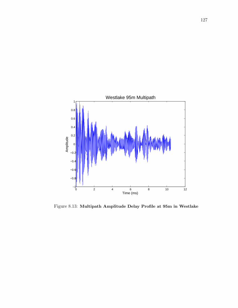
127
0 2 4 6 8 10 12−1
−0.8
−0.6
−0.4
−0.2
0
0.2
0.4
0.6
0.8
1
Time (ms)
Am
plitu
de
Westlake 95m Multipath
Figure 8.13: Multipath Amplitude Delay Profile at 95m in Westlake

128
8.3.5 Integrated System Test Summary
The integrated system test results in terms of distance, multipath delay
spread, bit error rate, and SNR are summarized in Figure 8.14. As anticipated,
the UCSDModem performed well (having a bit error rate of <5%) in environments
with a multipath spread less than 5 ms. The results also suggest that higher SNR
will only improve performance for environments with low multipath.
8.4 Summary
This chapter described the analog, digital and integrated system tests used
to evaluate the functionality and performance of the complete modem design.
These tests prove that a short-range underwater acoustic modem can be designed
from low-cost components. The tests indicate that the UCSDModem can support
data rates of 200 bps for ranges up to ∼400 meters with the power charcteristics
given in Table 9.2. Tables 4.1 and 4.2 show how the UCSDModem compares with
existing commercial and reseeach modems respectively.
The next chapter describes some deployment considerations one would have
to realize to use the UCSDModem in a practical short-range, low data-rate under-
water sensor network.
Selections of Chapter 8 are in part a reprint of the material as it appears
in the proceedings of the IEEE Oceans Conference. The dissertation author was
a co-primary researcher and author along with Ying Li, Brian Faunce, and Ken-
neth Domond. The other co-authors listed on this publication [1] directed and
supervised the research which forms the basis for Chapter 8.

129
Wes
tlake
: 5 m
, 2.0
ms
Tank
: 0.5
m, 1
.86
ms
Wes
tlake
: 50
m, 1
.5 m
s
Pool
: 50
m, 2
1.3
ms
Wes
tlake
: 380
m, x
ms
051015202530
05
1015
2025
3035
BER (%)
SNR
(dB)
Syst
em T
est R
esul
ts
"Loc
atio
n:
Dis
tanc
e,
Mul
tipat
h Sp
read
"
Fig
ure
8.14
:S
yst
em
Test
Resu
lts

Chapter 9
Deployment Considerations
Now that we have described the full modem design and tested its perfor-
mance, this chapter discusses some deployment considerations one would have to
realize to use the modem in a practical underwater sensor network. We begin
by describing a linear programming model that can be used to determine the re-
quired energy, cost, and lifetime of modems deployed on a given linear network.
We then discuss battery, housing, and marine life considerations for underwater
deployment.
9.1 Linear Programming Model
In order to determine the cost and energy requirements of modems on a
given linear network, we use a linear programming model, modified from [156]
with one of three objectives:
• Maximizing the lifetime of the network
• Minimizing the total energy consumption of the network
• Minimizing the total cost of the network
The model is given below:
130
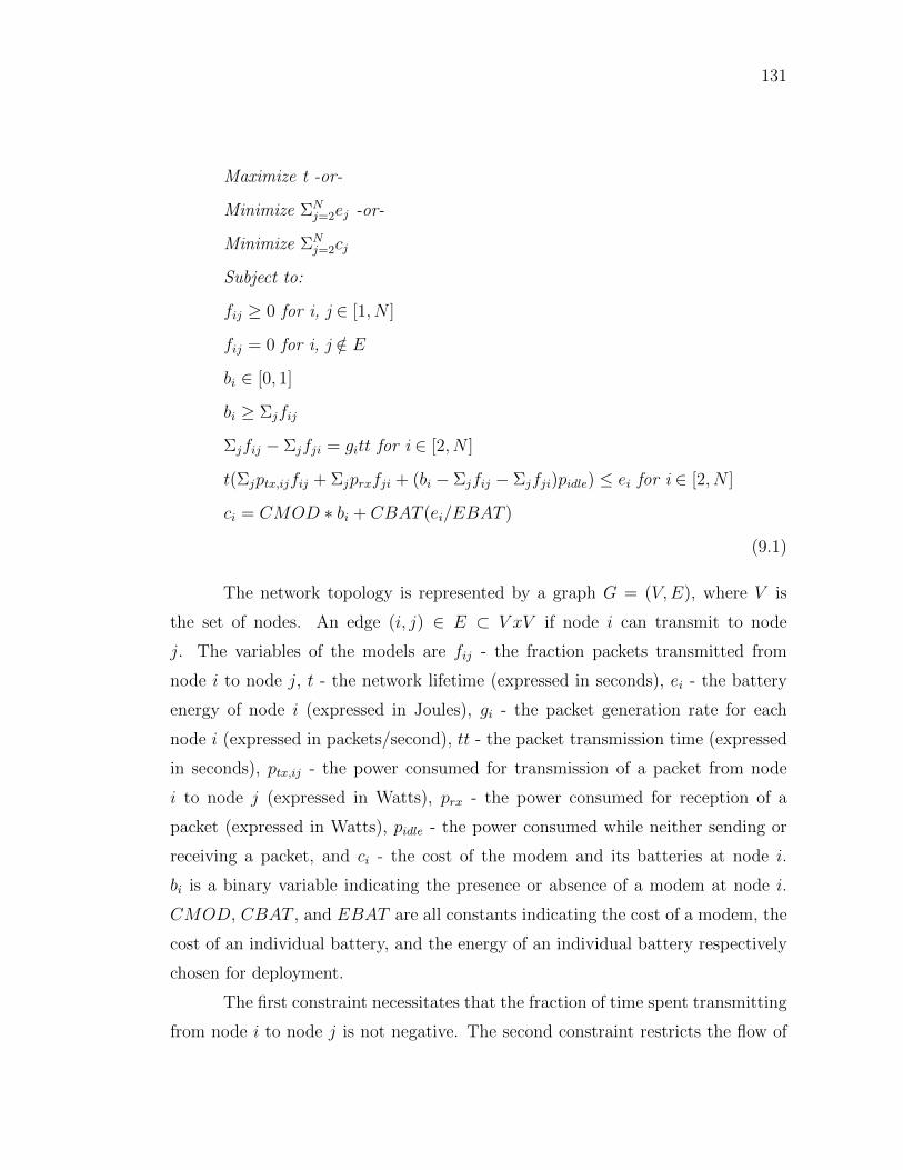
131
Maximize t -or-
Minimize ΣNj=2ej -or-
Minimize ΣNj=2cj
Subject to:
fij ≥ 0 for i, j ∈ [1, N ]
fij = 0 for i, j /∈ E
bi ∈ [0, 1]
bi ≥ Σjfij
Σjfij − Σjfji = gitt for i ∈ [2, N ]
t(Σjptx,ijfij + Σjprxfji + (bi − Σjfij − Σjfji)pidle) ≤ ei for i ∈ [2, N ]
ci = CMOD ∗ bi + CBAT (ei/EBAT )
(9.1)
The network topology is represented by a graph G = (V,E), where V is
the set of nodes. An edge (i, j) ∈ E ⊂ V xV if node i can transmit to node
j. The variables of the models are fij - the fraction packets transmitted from
node i to node j, t - the network lifetime (expressed in seconds), ei - the battery
energy of node i (expressed in Joules), gi - the packet generation rate for each
node i (expressed in packets/second), tt - the packet transmission time (expressed
in seconds), ptx,ij - the power consumed for transmission of a packet from node
i to node j (expressed in Watts), prx - the power consumed for reception of a
packet (expressed in Watts), pidle - the power consumed while neither sending or
receiving a packet, and ci - the cost of the modem and its batteries at node i.
bi is a binary variable indicating the presence or absence of a modem at node i.
CMOD, CBAT , and EBAT are all constants indicating the cost of a modem, the
cost of an individual battery, and the energy of an individual battery respectively
chosen for deployment.
The first constraint necessitates that the fraction of time spent transmitting
from node i to node j is not negative. The second constraint restricts the flow of

132
packets to only those nodes where transmission between node i and node j is
possible. The third constraint defines the variables, bi to be binary. The fourth
constraint indicates a node is present if it sends data to any of the other nodes.
The fifth constraint indicates the fraction of packets leaving node i must equal the
fraction of packets received at node i plus the fraction of packets generated at node
i. The sixth constraint indicates that the amount of power consumed receiving
packets at node i plus the amount of power consumed transmitting packets at node
i plus the amount of power consumed in an idle state over the network lifetime
must be less than or equal to the amount of energy available at node i. The final
constraint indicates that the cost of deploying a modem at node i is equal to the
cost of the modem (if the modem is present) plus the total number of batteries
required times the cost of a battery.
This model was written in Matlab using lp solve [157], a linear and mixed
integer/binary program solver based on the revised simplex method and the Branch-
and-bound method for integers. lp solve has no limit on model size and can be
called as a library from different languages such as C, VB, .NET, Excel, Java, and
Matlab.
In order to illustrate the use of the model, we apply it to a real applica-
tion scenario of the Santa Barbara Channel RelocaTable Mooring (CHARM). The
CHARM is a shallow water mooring located in 24 m water depth off the town of La
Conchita, CA (Figure 9.1). The CHARM has been retrieved and redeployed every
6 months since May 2003 with the purpose of: (1) developing and testing relatively
small, lightweight optical and chemical sensors and real time data telemetry for au-
tonomous deployment, (2) investigating particulate dynamics through optics, (3)
optical and chemical detection and characterization of harmful algal blooms, and
(4) determining effects of physical processes on chemical and bio-optical properties
[158].
The CHARM supports RF telemetry from its location, 2 km from shore,
to a shorebased data receiving station within line-of-sight and the 4 m instrument
package is hard-wired to the surface buoy, but has been subject to failure. Ideally,
all subsurface data would be transmitted to the surface buoy to be telemetered
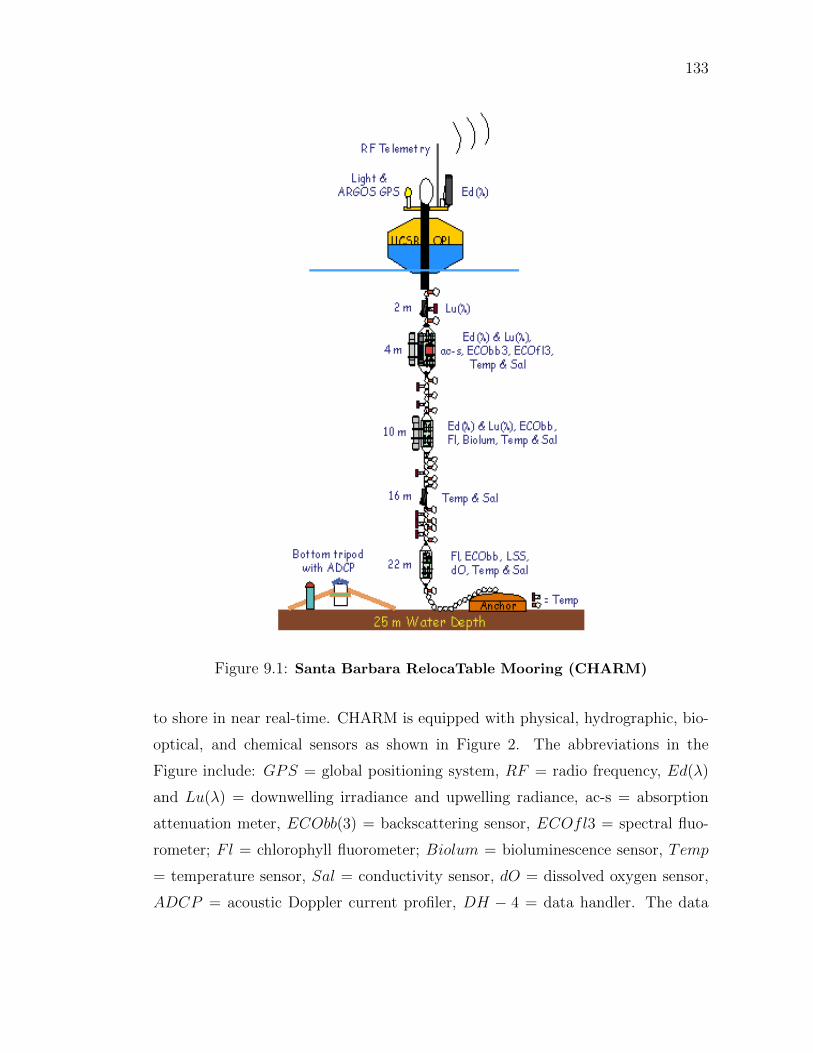
133
Figure 9.1: Santa Barbara RelocaTable Mooring (CHARM)
to shore in near real-time. CHARM is equipped with physical, hydrographic, bio-
optical, and chemical sensors as shown in Figure 2. The abbreviations in the
Figure include: GPS = global positioning system, RF = radio frequency, Ed(λ)
and Lu(λ) = downwelling irradiance and upwelling radiance, ac-s = absorption
attenuation meter, ECObb(3) = backscattering sensor, ECOfl3 = spectral fluo-
rometer; Fl = chlorophyll fluorometer; Biolum = bioluminescence sensor, Temp
= temperature sensor, Sal = conductivity sensor, dO = dissolved oxygen sensor,
ADCP = acoustic Doppler current profiler, DH − 4 = data handler. The data

134
sampling rates for major sensors and sensor packages on CHARM are shown in
Table 9.1.
Table 9.1: Data amounts for major sensors and sensor packages on the CHARM
Depth and Sensor or Amount Data Node NumberSensor Package (per day)1 m SBE 39 40 kB 2Temperature Sensor2 m Hyperspectral 130 kB 3Sensor4 m Sensor Package 450 kB 47 m SBE 39 40 kB 5Temperature Sensor10 m Sensor Package 325 kB 619 m SBE 39 40 kB 7Temperature Sensor22 m Sensor Package 65 kB 8
We use the data and distance parameters specified in Table 9.1 plus the
power parameters specified in 9.2 (that combine the analog and digital hardware
transmit, receive and idle power) as inputs to the linear programming model. We
assume that the surface node (Node 1) can be solar powered and therefore do not
report battery requirements for this node. The power to transmit from node i
to node j is governed by the distance between the nodes, i.e. larger powers are
required to transmit longer distances. In this particular application, all nodes
could be reached with the lowest power level as the maximum distance between
nodes is 22 meters. If distances were longer between nodes, additional nodes could
be placed inbetween data nodes to act as repeaters and possibly reduce power
consumption through multiple transmissions over shorter distances.
Table 9.2: UCSDModem Power Characteristics
Function Power (W)Tx 1.3-7.0RX 0.42Idle 0.33
Figure 9.2 and Table 9.3 show the routing, energy and cost results respec-
tively of the linear programming model for minimizing battery energy and cost

135
for a deployment time of 6 months assuming a modem cost of $500, an a cost per
joule of $10/70000 Joules. The modem cost was estimated using the parts cost of
the modem given in the bill of materials and an estimated cost of a shallow water
housing given in the following subsection. The battery cost and energy capacity
was estimated from the cost and energy capacity of a standard C cell battery.
Because the maximum transmit distance is 22 m, (a distance that can be handled
by the lowest power of the modem) the routing scheme requires each node to send
its data directly to the surface node.
Figure 9.2: Routing schemes for optimal cost and energy (for 6 month de-ployment) or lifetime (for 140kJ of energy) on the CHARM

136
Table 9.3: Minimum Energy and Cost Requirements for a 6 month deployment ofthe CHARM mooring
Node Energy Cost(kJ) ($)
1 5002 5172 1238.83 5190 1241.54 5257 12515 5171 1238.86 5231 1247.37 5171 1238.88 5176 1239.5Total 36370 8695.7
Figure 9.2 also shows the routing results of the linear programming model
for maximizing the network lifetime, giving each node only 140kJ of energy. The
maximum network lifetime for the SB CHARM deployed with the UCSDModem
is 4.7 days. Reducing the idle power to 500uW (as per [77]) would increase the
network lifetime to 6 months.
With these results, we see that the model is useful for giving a cost and
energy requirement estimate for outfitting a given linear underwater network with
a given acoustic modem. Note that the cost and energy estimates do not include
costs associated with deploying the network, costs or energy associated with the
network sensors themselves, nor cost and energy required for any possible packet
loss. The model is also useful for determining the amount of energy savings a given
reduction in transmit, receive, or idle power may provide in a practical application
scenario.
9.2 Battery Considerations
Any practical underwater modem deployment requires a battery pack to
provide power to the modem. Commercial modem companies sell battery packs
separately so users can select the type, size, form factor, and energy capacity of
the batteries for a given deployment. Users often select to purchase rechargeable
batteries so they can reuse the batteries for more than one deployment. Popular

137
rechargeable batteries include rechargeable alkaline batteries, lithium ion (Li-ion)
batteries, and nickel metal hydride (NiMH) batteries.
Rechargeable alkaline batteries cannot be recharged nearly as many times
as NiMH or Li-ion batteries, and lose charge capacity after just a few charges,
but are typically the least expensive of the rechargeable batteries. Li-ion batteries
have a higher energy density, have a lower self discharge rate (they will retain their
charge for a longer time), and can be smaller and lighter than most other types
of rechargeables. However, because Li-ion batteries require special circuitry to
protect the battery from damage due to undercharging or overcharging, they are
typically more expensive than other rechargeables and require custom (and thus
more expensive) chargers. Li-ion batteries are not available in standard cell sizes
(like AA, C, and D) to ensure they are not placed in chargers that could damage
the battery. NiMH batteries come in standard sizes, are less expensive than Li-ion
batteries, can be rapidly recharged over 500 times, and have higher energy density
than alkaline batteries (although less energy density than Li-ion batteries). Li-ion
are usually preferred if the budget allows, but NiMH are suitable if a standard
cell size is desired and cost is of importance. Standard C cell NiMH batteries cost
∼$10 and provide 70000 J of energy.
9.3 Housing Considerations
Any practical underwater modem deployment also requires a water-proof
housing rated to the depth of the deployment. The housing serves as both a mount-
ing platform and a watertight casing for all the modem components. Commercial
modem companies often sell housing separately so users can select the type, size,
form factor, and depth rating needed for a given deployment. Housings that can
withstand pressures at deeper depths are much more expensive than housings de-
signed for shallow water deployments.
Typical underwater modem housings are made out of plastics rated to with-
stand pressures at a given depth. Pressures increase by 1 bar for every 10 meters
below sea level, or 1 atmosphere for every 33 feet of sea water, so pressure at 100

138
meters reaches about 150 psi. These plastics also have high UV resistance as UV
radiation causes plastics to become brittle and fail overtime. Some housings are
made of UV resistant plastics such as Delrin (acetyl copolymer), or PEEK and
for a 1” diameter rod stock cost $4.50 and $60.00 per foot respectively. Non UV
resistant plastics such as PVC or ABS can be used as a low-cost alternative for
short deployments. Schedule 80 3” PVC pipe is rated to a maximum operating
pressure of 158 psi and costs roughly $3 per foot. The size of the housing must be
large enough to contain the modem hardware, batteries, and heat sink to reduce
thermal dissipation.
All that being said, the hard part (and most expensive) is not the plastic
tube used for the housing, but the required end caps and sealing hardware. Deflec-
tions in end caps become larger by r4, so keeping a relatively small tube diameter
is desirable to avoid increased trouble with sealing. An estimate for an end cap
designed for a 3” PVC pipe is $100. O-rings and stainless steel nuts and bolts are
used for sealing which cost on the order of $20-$50 depending on the design. Given
these cost estimates, a 3” PVC housing for the UCSDModem would cost ∼$150.
9.4 Marine Life Considerations
Any practical underwater modem deployment also requires attention to its
effect on marine life and the marine life’s effect on the modem. Care must be
paid to minimize the physical and acoustic interference between the modem and
its surrounding environment.
9.4.1 Physical Effects
A modem deployed in marine environment will be subjected to biofouling
- the undesirable accumulation of microorganisms, plants, algae, and/or animals
on wetted structures. Barnacles or algae could build up on a transducer poten-
tially blocking the modems signal and corrupting data. Anti-fouling techniques
such as applying an anti-fouling coating, should be considered especially for long
deployments.

139
Underwater instrumentation has also been known to suffer from shark bites
and other physical damage from curious marine animals, thus protective cages
should be considered depending on the deployment location and its inhabitants.
9.4.2 Acoustic Effects
Many marine animals use sound underwater including whales, dolphins,
certain species of fish (such as the toadfish), and certain species of marine inverte-
brates (such as snapping shrimp). Marine organisms use sound to communicate,
navigate and feed, using frequencies as low as 10Hz and as high as a few hundred
kilohertz. Marine organisms communicating in the operating frequency band of
an acoustic modem add to the ambient noise level in that band thus possibly cor-
rupting signal transmission. Marine mammal calls have been known to increase
ambient noise levels by 20-25 dB in the frequency band below 500 Hz and snap-
ping shrimp have been known to corrupt signal transmission in the 2-15KHz band
having individual source levels of 189 dB re 1 uPa at 1 meter (almost 50dB higher
than the source level of our modem) [159]. Researchers can devise higher level
networking protocols to counter the effects of marine life noise (i.e. retransmit
when the noise source is absent) should the signal be corrupted by an organism
producing sound in the modem’s operating frequency band.
Acoustic modems on the other hand, must be designed not to cause phys-
iological damage to marine organisms. Richardson et. al have shown that sound
levels of 195-210 dB re 1 uPa may cause immediate damage to the auditory organs
of baleen whales [162]. Simmonds and Hutchinson stated that intense underwa-
ter sound sources caused hemorrhage in the lungs and ulceration of the gastro-
intestinal tract for animals with air filled lungs or swim bladders [160]. In 1998,
the Seattle Times reported hundreds of dead fish appeared in Lake Washington
after 240 dB re 1 uPa airgun blasts were used to test for earthquake faults [161].
The UCSDModem operates at source levels well under those that have been shown
to cause damage to marine life.

140
9.5 Summary
This chapter described a linear programming model that optimizes for cost,
energy consumption or deployment time for a given linear underwater network
equipped with acoustic modems, and described battery, housing, and marine life
considerations. The linear programming model was used to equip an existing un-
derwater network, the CHARM, with the UCSDModem to illustrate the modem’s
potential use, energy, cost and lifetime requirements in a practical real-life scenario.
The next chapter describes some future improvements that could be made to the
modem to make it more versatile for a wider variety of sensor network applications
and underwater environments.

Chapter 10
Future Improvements
This thesis described the design and initial testing of a functional low-cost
underwater acoustic modem prototype for short-range underwater sensor networks.
The UCSDModem can support data rates of 200 bps for ranges up to ∼400 meters
in environments with less that 5 ms multipath delay spread. This chapter discusses
possible future improvements to the modem to make it more versatile for a wider
variety of sensor network applications and underwater environments.
Power Reduction: The linear programming model described in Chapter
9 showed the necessity of reducing power consumption (particularly idle power
consumption) to ensure a longer deployment lifetime on a limited battery supply.
Further improvements could be made to the analog and digital transceivers to
make them more power efficient and a low power wake up circuit could be added
to greatly reduce listening/idle power.
Wider Bandwidth, Higher Bit Rate: The existing FSK modulation
scheme uses only a 1 kHz bandwidth which achieves a theoretical maximum bit
rate of 500 bps and a practical bit rate of 200 bps. As the transducer is power
efficient over a 5 kHz band (see Figure 6.9), the bandwidth of the receiver could be
widened to amplify signals over the 5 kHz range allowing for a modulation scheme
that uses more bandwidth allowing higher data rates. However, the widening of
the receiver bandwidth comes at a cost of reducing gain, thus reducing transmis-
141

142
sion range.
Low-Power DSP: The existing digital transceiver design was implemented
on a FPGA that provides comparable power consumption to other low power re-
search modem designs. Because the FPGA does not offer considerable power
savings over the other designs (see Table 7.4) and because FPGA design time is
so high, it may make sense to move the design to a low-power DSP. DSPs can be
much more easily configured and reprogrammed allowing the user to easily modify
the modulation scheme and its parameters.
Channel Adaptive Modem: As shown in the system test results, the
current modem design can only perform well in environments with a low multi-
path delay spread. An adaptive algorithm could be programmed into the mo-
dem to measure the channel characteristics and apply channel equalization and/or
lengthen the symbol period for channels with high multipath.
The ideas conveyed in the thesis are shared with the material in the pro-
ceedings of the IEEE Oceans Conference and the Embedded Systems Letters. The
dissertation author was a co-primary researcher and author along with Ying Li,
Brian Faunce, and Kenneth Domond. The other co-authors listed on these publi-
cations [1, 2] directed and supervised the research which forms the basis for the
dissertation.

Appendix A
Bill Of Materials
Table A.1 shows the bill of materials for the UCSDModem providing parts
costs for the transducer, analog transceiver, and digital transceiver. Low volume
costs are estimated for purchasing quantities of components for fewer than 50
modems. High volume costs are estimated for purchasing components in bulk (for
some components such as resistors and capacitors that means quantities greater
than 1000). Digital costs are estimated for a custom digital board that use the
EP4CE30 FPGA and required peripherals.
143

144
Table A.1: Underwater Modem Bill of Materials
Transducer ComponentsPart Quantity High Volume ($) Low Volume ($)Ceramic 1 10 10Potting Compound 3 oz 10 10Shielded cable 2” 1 11/4” cork sheet 1 6 61/8” cork sheet 1 13 13Mold 1 2 2Total 6 42 42Analog ComponentsPart Quantity High Volume ($) Low Volume ($)Resistors 92 16 17Capacitors 76 32 54Diodes 7 42 5Mosfets 4 3 4Comparator 1 1 2Op Amps 12 36 53Relays 6 28 40Connectors 28 13 20Ferrite Cores 3 5 7Wires 4 4 4Board 1 50 20Total 234 162 248Digital ComponentsPart Quantity High Volume ($) Low Volume ($)FPGA 1 40 60UART 1 2 5ADC 1 2 4DAC 1 5 7Connectors various 10 20Digital Board 1 5 15Total 6 148 195Grand Total 246 ∼350 <500

Bibliography
[1] B. Benson, Y. Li, B. Faunce, K. Domond, D. Kimball, C. Schurgers, and R.Kastner, Design of a Low-Cost, Underwater Acoustic Modem for Short-RangeSensor Networks, IEEE Oceans Conerence, 2010.
[2] B. Benson, Y. Li, B. Faunce, K. Domond, D. Kimball, C. Schurgers, and R.Kastner, Design of a Low-Cost Underwater Acoustic Modem, Embedded Sys-tems Letters, accepted.
[3] Y. Li, B. Benson, X. Zhang, and R. Kastner, Hardware Implementation ofSymbol Synchronization for Underwater FSK, IEEE International Conferenceon Sensor Networks, Ubiquitous, and Trustworthy Computing, 2010.
[4] R. Beckwith, D. Teibel, and P. Bowen, Unwired wine: Sensor networks invineyards, In Proceedings of IEEE Sensors, 2004.
[5] A. Mainwaring, J. Polastre, R. Szewczyk, and D. Culler, Wireless sensor net-works for habitat monitoring, In Proceedings of the ACM Workshop on SensorNetworks and Applications, September 2002.
[6] J. Lynch, K. Law, E. Straser, A. Kiremidjian, and T. Kenny, The Develop-ment of a Wireless Modular Health Monitoring System for Civil Structures,Proceedings of the MCEER Mitigation of Earthquake Disaster by AdvancedTechnologies Workshop, November 2000.
[7] N. Ramanathan, M. Yarvis, J. Chhabra, N. Kushalnagar, L. Krishnamurthy,and D. Estrin, A stream-oriented power management protocol for low dutycycle sensor network applications, In Proceedings of the IEEE Workshop onEmbedded Networked Sensors, May 2005.
[8] J. Heidemann, W. Ye, J. Wills, A. Syed, and Y. Li, Research challenges andapplications for underwater sensor networking, Proceedings of IEEE WirelessCommunications and Networking Conference (WCNC), pp. 263-70, 2006
145

146
[9] D. Codiga, J. A. Rice, and P. S. Bogden, Real-time wireless delivery of sub-surface coastal circulation measurements from distributed intruments usingnetworked acoustic modems, Proceedings of MTS/IEEE Oceans 2000, 2000.
[10] J. G. Proakis, E. M. Sozer, J. A. Rice, and M. Stojanovic, Shallow wateracoustic networks, IEEE Communications Magazine, pp. 114-119, 2001.
[11] E. M. Sozer, M. Stojanovic, and J. G. Proakis, Underwater acoustic networks,IEEE Journal of Oceanic Engineering, vol. 25, pp. 72-83, 2000.
[12] H. Milburn, A. Nakamura, and F.I. Gonzalez, DeepoceanAssessment and Reporting of Tsunamis (DART): Real-TimeTsunami Reporting from the Deep Ocean, NOAA Online Report,http://www.ndbc.noaa.gov/Dart/milburn 1996.shtml, 1996.
[13] Ocean Research Interactive Observatory networks Website (ORION),http://www.orionprogram.org.
[14] Laboratory for the Ocean Observatory Knowledge Integration Grid (LOOK-ING) Website, http://lookingtosea.ucsd.edu.
[15] Monterey Accelerated Research System (MARS) Website,http://www.mbari.org/mars/.
[16] NEPTURE Website, http://www.neptune.washington.edu.
[17] D. Estrin, L. Girod, G. Pottie, and M. Srivastava, Instrumenting the worldwith wireless sensor networks, IEEE International Conference on Acoustics,Speech, and Signal Processing, 2001.
[18] J. M. Rabaey, M. J. Ammer, J. L. da Silva, D. Patel, and S. Roundy, Pico-Radio supports ad-hoc ultra-low power wireless networking, IEEE Computer,pp. 42-48, 2000.
[19] I. F. Akyildiz, D. Pompili and T. Melodia, Challenges for Efficient Commu-nication in Underwater Acoustic Sensor Networks, ACM Sigbed Review, Vol.1, No. 2, July 2004.
[20] R. Jurdak, C. V. Lopes, and P. Baldi, Battery lifetime estimation and op-timization for underwater sensor networks, in Sensor Network Operations, S.Phoha, T. F. LaPorta, and C. Griffin, Eds.: IEEE Press, 2004.
[21] R. Galzin and J. P. Pointier, Moorea island, Societyarchipelago, Proceedings

147
of the 5th International Coral Reef Congress, vol. 1, pp. 73-102., 1985.
[22] J. Jaffe and C. Schurgers, Sensor networks of freely drifting autonomous un-derwater explorers, Proceedings of ACM International Workshop on Underwa-ter Networks, 2006.
[23] J. Jaffe, R. Glatts, C. Schurgers, D. Mirza, P. Franks, P. Roberts, and F. Si-monet, AUE: An Autonomous Float for Monitoring the Upper Water Column,in Proceedings of MTS/IEEE Oceans 2007, Aberdeen, Scotland, 2007.
[24] D. Mirza and C. Schurgers, Collaborative localization for fleets of underwaterdrifters, in MTS/IEEE Oceans, October 2007.
[25] G. Chang, T. Dickey, and M. Lewis, Toward a global ocean system for mea-surements of optical properties using remote sensing and in situ observations,Remote Sensing of the Marine Environment, vol. 6, pp. 285-326, 2006.
[26] D. Frye, L. Freitag, R. Detrick, J. Collins, J. Delaney, D. Kelley, A. LaBonte,and K. Brown, An acoustically linked moored-buoy ocean observatory, EOS,87(22), 2006.
[27] A., Hamilton, M. Chaffey, E. Mellinger, J. Erickson, and L. McBride, Dynamicmodeling and actual performance of the MOOS test mooring, Proceedings ofMTS/IEEE Oceans, 2006.
[28] Real-Time Oceanography with Inductive Moorings, Sea-Bird Electronics, Inc.,http://www.seabird.com/technical references/IMtutorialR2.htm.
[29] B. Benson, F. Spada, D. Manov, G. Chang and R. Kastner, Real Time Teleme-try Options for Ocean Observing Systems, European Telemetry Conference,April 2008.
[30] Electromagnetic Wave, Def, American Heritage Dictionary of the English Lan-guage, 4th ed.
[31] J.B. Lindsay, Mr. Lindsay’s marine telegraph, Dundee Advertiser, 12th April1853.
[32] M. Siegel and R. W. P. King, Electromagnetic propogation between antennassubmerged in the ocean, IEEE Trans. Antennas Progagation, vol. 4, pp. 507-513, 1973.
[33] M. Rhodes, Electromagnetic Propagation in Sea Water and its value in Mil-

148
itary Systems, Second Annual Conference of Systems Engineering for Au-tonomous Systems, July 2007.
[34] L. Butler, Underwater Radio Communication, Amateur Radio, April 1987.
[35] R. Moore, Radio Communications in the Sea, lEEE Spectrum, Vol 4, pp 42-51,Nov 1967.
[36] T. Shelley, Radio waves transmit information underwater, An article in EurekaMagazine, Nov. 14, 2005.
[37] Extremely Low Frequency Transmitter Site ClamLake, Wisconsin, United States Navy Fact File,http://enterprise.spawar.navy.mil/UploadedFiles/fs clam lake elf2003.pdf
[38] A. I. Al-Shamma’a, A. Shaw, and S. Saman, Propagation of electromagneticwaves at MHz frequencies through seawater, IEEE Transactions on Antennasand Propagation, vol. 52, no. 11, pp. 2843-2849, Nov. 2004.
[39] J. Lucas, A. Al-Shamma’a, J. Seim, W. Loehr, G. Puchbauer, and D. McGre-gor, Underwater communications using electromagnetic waves (EMCOMMS),in Proceedings of European Conference on Marine Science and Ocean Technol-ogy, 2004.
[40] Wireless Fibre Systems, http://www.wirelessfibre.co.uk/.
[41] R. Stewart, Introduction to Physical Oceanography, Texas A & M University,September 6, 2005.
[42] L. Liu, S. Zhou and J.-H. Cui, Prospects and problems of wireless communi-cation for underwater sensor networks, Wireless Communications and MobileComputing, pp. 977-994, 2008.
[43] Y. Ito, S. Haruyama, and M. Nakagawa, Short-Range Underwater WirelessCommunication Using Visible Light LEDs, IEICE, 2006.
[44] J. R. Apel, Principles of Ocean Physic,International Geophysics Se-ries,Academic Press, Vol. 38, pp509-584, 1987.
[45] H. Arst, Optical Properties and Remote Sensing of Multicomponental WaterBodies, Praxis Publishing, Chichester, UK, pg 8-28, 2003.
[46] M. Chancey, Short Range Underwater Optical Communication Links, North

149
Carolina State University, Masters Thesis, 2005.
[47] M. Kerker, The Scattering of Light and other Electromagnetic Radiation, 3rdEd. Academic Press, New York, NY, 1973.
[48] N.G. Jerlov, Optical Oceanography, Elsevier Publishing Company, New York,Vol. 5, pg 50-62, 118-126, 1968.
[49] Underwater Laser Pops in Navy Ops. BBC News. 8 September 2009.
[50] I. Vasilescu, K. Kotay, D. Rus, M. Dunbabin, and P. Corke, Data collection,storage, and retrieval with an underwater sensor network, Proceedings of ACMSensys, 2005.
[51] F. Schill, U.R. Zimmer, J. Trumpf, Visible spectrum optical communicationand distance sensing for underwater applications, The Australasian ConferenceRobotics and Automation ACRA, 2004.
[52] N. Farr, A. Chave, L. Freitag, J. Preisig, S. White, and D. Yoerger, Opticalmodem technology for seafloor observatories, Oceans, 2005.
[53] J. Simpson, A 1 Mbps Underwater Communication System using LEDs andPhotodiodes with Signal Processing Capability, North Carolina State Univer-sity, Masters Thesis, 2007.
[54] F. Hanson and S. Radic, High bandwidth underwater optical communication,Applied Optics, vol. 47, pp. 277283, Jan. 2008.
[55] P. J. Westervelt and R. S. Larson, Laser-excited broadside array, Journal ofthe Acoustic Society of America, vol. 54, pp. 121122, 1973.
[56] Y. H. Berthelot, Thermoacoustic generation of narrow-band signals with highrepetition rate pulsed lasers, Journal of the Acoustic Society of America, vol.85, pp. 11731181, 1989.
[57] F. Blackmon, L. Estes, and G. Fain, Linear opto-acoustic underwater com-munication, Applied Optics, vol. 44, no. 18, pp. 38333845, Jun. 2005.
[58] M. A. Ainslie and J. G.McColm, A simplified formula for viscous and chemicalabsorption in sea water, Journal of the Acoustical Society of America, vol. 103,no. 3, pp. 16711672, 1998.
[59] F. Fisher and V. Simmons, Sound Absorption in Sea Water, Journal of the

150
Acoustical Society of America, vol. 62, no. 3, pp. 558-564, 1977.
[60] R. Urick, Principles of Underwater Sound. 3rd ed. New York: McGraw-Hill,1983.
[61] National Research Council (NRC), Ocean Noise and Marine Mammals. Na-tional Academies Press, 2003.
[62] G.M. Wenz, Acoustic ambient noise in the ocean: Spectra and sources, Journalof the Acoustical Society of America, 34, 19361956, 1962.
[63] J. Preisig, Acoustic propagation considerations for underwater acoustic com-munications network development,Proceedings of First ACM InternationalWorkshop on Underwater Networks, Sep. 2006.
[64] M. Stojanovic, On the relationship between capacity and distance in an under-water acoustic communication channel, Proceedings of First ACM InternationalWorkshop on Underwater Networks, Sep. 2006.
[65] M. Stojanovic, Underwater Acoustic Communications, Encyclopedia of Elec-trical and Electronics Engineering, John G. Webster, Ed., John Wiley & Sons,vol.22, pp.688-698. 1999.
[66] Underwater Acoustic Propagation Modelling Software - AcTUP V 2.2L,http://cmst.curtin.edu.au/products/actoolbox.cfm.
[67] D. B. Kilfoyle and A. B. Baggeroer, The state of the art in underwater acoustictelemetry, IEEE Journal of Oceanic Engineering, vol. 25, no. 1, pp. 427, Jan.2000.
[68] F. Tong, B. Benson, Y. Li, and . Kastner, Channel Equalization Based onData Reuse LMS Algorithm for Shallow Water Acoustic Communication, IEEEInternational Conference on Sensor Networks, Ubiquitous, and TrustworthyComputing, June 2010.
[69] LinkQuest, Inc., Underwater acoustic modems, http://www.link-quest.com/html/models1.htm.
[70] Benthos, Inc., Acoustic Modems, http://www.benthos.com/acoustic-telesonar-modem-product-comparison.asp.
[71] Tritech International, Tritech Micron Data Modem - Small ROV Communi-cations, http://www.tritech.co.uk/products/products-micron modem.htm.

151
[72] Aquatec Group, AQUAmodem 500 Overview,http://www.aquatecgroup.com/aquamodem.html.
[73] EvoLogics, Underwater Acoustic Modemhttp://www.evologics.de/en/products/acoustics/index.html.
[74] DSPComm, AquaComm: Underwater wireless modem,http://www.dspcomm.com/products aquacomm.html.
[75] L. Freitag, M. Grund, S. Singh, J. Partan, P. Koski, and K. Ball, The WHOImicro-modem: an acoustic communications and navigation system for multipleplatforms, MTS/IEEE OCEANS, pp. 1086-92 Vol, 2005.
[76] Hydro International, Product Survey: Acoustic Modems, http://www.hydro-international.com/files/productsurvey v pdfdocument 15.pdf, June 2007.
[77] J. Wills, W. Ye, and J. Heidemann, Low-power acoustic modem for denseunderwater sensor networks, Proceedings of ACM International Workshop onUnderwater Networks, 2006.
[78] R. Jurdak, C.V. Lopes, and P. Baldi. Software Acoustic Modems for ShortRange Mote-based Underwater Sensor Networks, Proceedings of IEEE OceansAsia Pacific, May 2006.
[79] MoteIV Corporation, www.moteiv.com.
[80] R. A. Iltis, H. Lee, R. Kastner, D. Doonan, T. Fu, R. Moore and M. Chin.An Underwater Acoustic Telemetry Modem for Eco-Sensing, Proceedings ofMTS/IEEE Oceans, September 2005.
[81] T. Fu, D. Doonan, C. Utley, B. Benson, R. Kastner, R. A. Iltis, and H. Lee,AquaModem Field Tests in Moorea, Poster Presentation, Proceedings of ACMInternational Workshop on Underwater Networks, September 2007.
[82] J. Namgung, N. Yun, S. Park, C. Kim, J. Jeon, and S. Park, Adaptive MACProtocol and Acoustic Modem for Underwater Sensor Networks, Demo Presen-tation, Proceedings of ACM International Workshop on Underwater Networks,November 2009.
[83] I. Vasilescu, C. Detweiler, and D. Rus, AquaNodes:An Underwater SensorNetwork, Proceedings of ACM International Workshop on Underwater Net-works, September 2007.

152
[84] H. Yan, S. Zhou, Z. Shi, and B. Li, A DSP Implementation of OFDM Acous-tic Modem, Proceedings of ACM International Workshop on Underwater Net-works, September 2007.
[85] S. Zhou, Z. Shi, J. Cui, H. Zhou, J. Liu, and P. Carroll, Aqua-fModem: AStand-alone Underwater Acoustic Modem Based on OFDM Technology, DemoPresentation, November, 2009.
[86] Z. Yan, J. Huang, C. He, Implementation of an OFDM underwater acous-tic communication system on an underwater vehicle multiprocessor structure,Frontiers of Electrical and Electronic Engineering in China, vol. 2, no. 2, pp.151-155, April 2007.
[87] E. M. Sozer and M. Stojanovic, Reconfigurable Acoustic Modem for Under-water Sensor Networks, Proceedings of ACM International Workshop on Un-derwater Networks, 2006.
[88] M. Vajapeyam, U. Mitra, J. Preisig, and M. Stojanovic, Distributed TR-STBC schemes for cooperative underwater acoustic communications, Proceed-ings of Oceans06 Asia Pacific, May 2006.
[89] P. Ozog, M. Lesser, M. Stojanovic, Adapting the USRP as an UnderwaterAcoustic Modem, Poster Presentation, High Performance Embedded Comput-ing, September 2009.
[90] P. J. Gendron, Orthogonal frequency division multiplexing with on-off-keying:Noncoherent performance bounds, receiver design and experimental results,U.S. Navy Journal of Underwater Acoustics, vol. 56, no. 2, pp. 267300, Apr.2006.
[91] M. Stojanovic, Low complexity OFDM detector for underwater channels, Pro-ceedings of MTS/IEEE OCEANS, September 2006.
[92] Cadence PSpice A/D and Advanced Analysishttp://www.cadence.com/products/orcad/pspice simulation/Pages/default.aspx
[93] B. Li, S. Zhou, M. Stojanovic, L. Freitag, and P. Willett, Multicarrier com-munication over underwater acoustic channels with nonuniform Doppler shifts,IEEE Journal of Oceanic Engineering, vol. 33, no. 2, Apr. 2008.
[94] B. Li, S. Zhou, M. Stojanovic, L. Freitag, and P. Willett, Non-uniform Dopplercompensation for zero-padded OFDM over fast-varying underwater acousticchannels, in Proceedings of MTS/IEEE OCEANS conference, Aberdeen, Scot-

153
land, Jun. 18-21, 2007.
[95] B. Li, S. Zhou, J. Huang, and P. Willett, Scalable OFDM design for underwa-ter acoustic communications, in Proceedings of Intl. Conf. on ASSP, Las Vegas,NV, Mar. 3 Apr. 4, 2008.
[96] T. Kang and R. A. Iltis, Matching Pursuits Channel Estimation for an Un-derwater Acoustic OFDM Modem, Proceedings of the 2008 IEEE Interna-tional Conference on Acoustics, Speech, and Signal Processing Special Sessionon Physcial Layer Challenges in Underwater Acoustic Communications, April2008.
[97] D. B. Kilfoyle, J. C. Preisig, and A. B. Baggeroer, Spatial modulation experi-ments in the underwater acoustic channel, IEEE Journal of Oceanic Engineer-ing, vol. 30, no. 2, pp. 406415, Apr. 2005.
[98] S. Roy, T. M. Duman, V. McDonald, and J. G. Proakis, High rate com-munication for underwater acoustic channels using multiple transmitters andspace-time coding: Receiver structures and experimental results, IEEE Journalof Oceanic Engineering, vol. 32, no. 3, pp. 663688, July 2007.
[99] B. Li, S. Zhou, M. Stojanovic, L. Freitag, J. Huang, and P. Willett, MIMO-OFDM over an underwater acoustic channel, Proceedings of MTS/IEEEOCEANS, September 2007.
[100] Sensor Design Fundamentals:Piezoelectric Transducer Design for MarineUse, Airmar Technology Corporation, 2000.
[101] Channel Industies Inc. Piezoelectric Ceramics Catalog, online document,www.channelindustries.com, Jun 2009.
[102] Piezo Theory, APC International Ltd.,http://www.americanpiezo.com/piezo theory/index.html.
[103] C.H. Sherman and J.L. Butler, Transducers and Arrays for UnderwaterSound, New York: Springer, 2007.
[104] Revision of DOD-STD-1376A, Ad Hoc Subcommittee Report on Piezoce-ramics, April 1986.
[105] MIL-STD-1376B (Notice 1), Military Standard Piezoelectric ceramic mate-rial and measurements guidelines for sonar transducers, July 1999.

154
[106] Morgan ElectroCeramics, http://www.morganelectroceramics.com.
[107] O.B. Wilson, An Introduction to Theory and design of Sonar Transducers,Peninsula Pub, 1985.
[108] Steminc, Steiner & Martins, Inc., http://www.steminc.com/.
[109] Cytec Industries, http://www.cytec.com/.
[110] Urethanes, Silicones, and Epoxies Seminar, Deep Sea Power and Light facil-ities, 4033 Ruffin Road, San Diego, CA 92123-1817, May 2009.
[111] How-To Guide for Mold Making and Casting, Smooth-On, www.smooth-on.com.
[112] R. Urick, Principles of Underwater Sound for Engineers, McGraw Hill BookCompany, 1967.
[113] W. MacLean, Absolute Measurement of Sound without a Primary Standard,Journal of the Acoustical Society of America, volume 12, pp 140-146, 1940.
[114] P. Ebaugh, and R. Meuser, Practical Application of the Reciprocity Theoremin the Calibration of Underwater Sound Transducers,Journal of the AcousticalSociety of America, volume 19, pp 695-700, 1947.
[115] B. Simmons and R. Urick, The Plane Wave Reciprocity Parameter and ItsApplication to the Calibration of Electroacoustic Transducers at Close Dis-tances, Journal of the Acoustical Society of America, volume 21, pp 633, 1949.
[116] R. Bobber and G.A. Sabin, Cylindrical Wave Reciprocity Parameter, Journalof the Acoustical Society of America, volume 33, pp 446, 1961.
[117] Marport Deep Sea Technology, http://www.marport.com/.
[118] ITC-1042, Deep Water Omnidirectional Transducer, http://www.itc- trans-ducers.com.
[119] H. Krauss, C. Bostian, and F. Raab, Solid State Radio Engineering, JohnWiley & Sons, 1980.
[120] J. Honda and J. Adams, Application Note AN-1071, International Recti-fier, Class D Audio Amplifier Basics, www.irf.com/technical-info/appnotes/an-1071.pdf

155
[121] Electronics Tutorial about Amplifiers, Electronics-Tutorials,http://www.electronics-tutorials.ws/amplifier/amp 1.html.
[122] C. Verhoeven, A. van Staveren, G. Monna, M. Kouwenhoven and E. Yildiz,Structured electronic design: negative feedback amplifiers, Boston/Dordrecht:Kluwer Academic, 2003.
[123] I. F. Akyildiz, D. Pompili, and T. Melodia, Underwater acoustic sensor net-works: research challenges, Ad Hoc Networks (Elsevier), 3(3):257–279, May2005.
[124] A. Phadke, Handbook of Electrical Engineering Calculations, Technologyand Engineering, 1999.
[125] M. Stojanovic, J. Catipovic, J.G. Proakis, Phase coherent digital communi-cations for underwater acoustic channels, IEEE Journal of Oceanic Engineering19 (1) (1994) 100111.
[126] L. Freitag, M. Stojanovic, S. Singh, and M. Johnson, Analysis of channeleffects on direct-sequence and frequency-hopped spreadspectrum acoustic com-munications, IEEE Journal of Oceanic Engineering, vol. 26, no. 4, pp. 586593,Oct. 2001.
[127] J. A. C. Bingham, Multicarrier modulation for data transmission: An ideawhose time has come, IEEE Communications Magazine, pp. 514, May 1990.
[128] Z. Wang and G. B. Giannakis, Wireless multicarrier communications: WhereFourier meets Shannon, IEEE Signal Processing Magazine, vol. 17, no. 3, pp.2948, May 2000.
[129] Analog Devices’ New Blackfin Family Offers the Fastest and MostPower-Efficient Processors for Their Class, Radio Locman, 2003.http://www.radiolocman.com/news/new.html?di=475.
[130] M. Yovits, Advances in computers, Academic Press, pp. 105-107, 1993.
[131] A. Amara, F. Amiel, and T. Ea, FPGA vs. ASIC for low power applications,Microelectronics Journal, v. 37, pp. 669-677, 2006.
[132] E. Rocha, Implementation Tradeoffs of Digital FIR filters, Military Embed-ded Systems, OpenSystems Publishing, 2007.
[133] R. Kastner, A. Kaplan, and M. Sarrafzadeh, Synthesis Techniques and Op-

156
timizations for Reconfigurable Systems. Boston: Kluwer Academic, 2004.
[134] W. Mangione-Smith , B. Hutchings , D. Andrews, A. DeHon , C. Ebeling, R. Hartenstein , O. Mencer , J. Morris, K. Palem , V. Prasanna , and H.Spaanenburg, Seeking Solutions in Configurable Computing, Computer, v.30n.12, pp. 38-43, December 1997.
[135] A. DeHon and J. Wawrzynek, Reconfigurable computing: what, why, andimplications for design automation, Proceedings 1999 Design Automation Con-ference, IEEE, pp. 610-15, 1999.
[136] K. Bondalapati and V. K. Prasanna, Reconfigurable computing systems,Proceedings of the IEEE, vol. 90, pp. 1201-17, 2002.
[137] K. Compton and S. Hauck, Reconfigurable computing: a survey of systemsand software, ACM Computing Surveys, vol. 34, pp. 171-210, 2002.
[138] P. Schaumont, I. Verbauwhede, K. Keutzer, and M. Sarrafzadeh, A quicksafari through the reconfiguration jungle, Proceedings of the 38th Design Au-tomation Conference (IEEE Cat. No.01CH37232). ACM. 2001, pp. 172-7.
[139] Micro-Modem Overview, Woods Hold Oceanographic Institution,http://acomms.whoi.edu/umodem/.
[140] D. Doonan, AquaModem Electronics Engineer, Personal Communication,May 2006.
[141] M. LaPedus. FPGAs can outperform DSPs, study says, DSP DesignLine,11/13/2006.
[142] BDTI, FPGAs vs. DSPs: A look at the unanswered questions, DSP DesignLine 1/11/2007.
[143] ModelSim SE 6.4a. http://model.com/content/modelsim-downloads.
[144] Spiral. http://spiral.net/hardware/filter.html.
[145] S. Bregni, Synchronization of Digital Telecommunications Networks, WI-LEY, 2002.
[146] E. M. Sozer and M. Stojanovic, Underwater Acoustic Networks, IEEE Jour-nal of Oceanic engineering, Vol. 25, No. 1, January 2000.

157
[147] C. Chien, Digital radio system on a chip: a system approach, Springer, 2001.
[148] B. Watson, FSK: Signals and Demodulation, W. J. Communications, July2004 ¡http://www.wj.com/pdf/technotes/FSK signals demod.pdf.
[149] FPGA and Programmable Logic Journal,http://www.fpgajournal.com/fpgajournal/feature articles/ 20090203 grand/.
[150] Altera’s New Cyclone IV, http://www.altera.com/corporate/news room/releases/2009/products/nr-cyclone-iv.html.
[151] DINI Group, DNMEG ADDA,http://www.dinigroup.com/index.php?product=DNMEG ADDA.
[152] M-Audio Ltd, http://www.m-audio.com.
[153] Xilinx Chipscope Pro, http://www.xilinx.com/tools/cspro.htm.
[154] H. Li, D. Liu, J. Li, and P. Stoica, Channel order and RMS delay spreadestimation with application to AC power line communications, Digital SignalProcessing, Vol. 13, pp 284-300, 2003.
[155] W. Dally and J. Poulton, Digital Systems Engineering, Cambridge UniversityPress, pp. 280285, 1998.
[156] S. Ergen and P. Varaiya, On multi-hop Routing for Energy Efficiency. Com-munications Letters, IEEE, Vol.9, Iss.10, Oct.2005, Pages: 880- 881.
[157] Using lpsolve from Matlab, http://lpsolve.sourceforge.net/5.5/MATLAB.htm.
[158] University of California Santa Barbara OceanPhysics Laboratory, CHAnnel Relocatable Mooring,(CHARM);http://www.opl.ucsb.edu/mosean/datasb.html.
[159] Sounds in the Sea: What are common underwa-ter sounds?, Discovery of Sound in the Sea Website,http://www.dosits.org/science/soundsinthesea/commonsounds/.
[160] M.P. Simmonds and J.D. Hutchinson, The Conservation of Whales and Dol-phins, John Wiley & Sons. 1996.
[161] USGS Fish Kill Investigation, USGS,http://walrus.wr.usgs.gov/earthquakes/ships/deadfish.html.

158
[162] W.J. Richardson, C.R. Green, C.I. Malme, D.H. Thompson, S.E. Moore,B. Wurwig, Effects of noise on marine mammals, Report prepared by LGLEcological Research Associates Inc., TX, for US Minerals Management Service,Study 90-0093, NTIS PB 91-168914, pp 462.