design of a direct neural braking system based on

IJCCCE Vol.13, No.3, 2013

____________________________________________________________________________________

15

Design of a Direct Neural Braking System based on

Switching Gains Controller

Dr. Hayder Sabah. Abdulamir Machines and Equipments Department, Institute of Technology, Baghdad

[email protected]

Received: 18/2/2013 Accepted: 12/11/2013

Abstract- In this paper, direct neural controller for braking system is proposed. Learning of the presented controller depends on the training data that comes from running the switching gain controller at different conditions of drive. The training data consist of relative velocity error, distance error and braking force. The feed-forward neural network is used to build direct neural controller with two hidden layers and using back-propagation training algorithm. The performance of the presented controller is validated using nonlinear braking model. Simulation results show the presented controller is able to prevent the collision of vehicles at different driving conditions. Also, the results show superiority of the direct neural controller in comparison with the switching gain controller at all drive cases that are tested in this work.

Keywords – Switching Controller, Neural Network, Braking System.

IJCCCE Vol.13, No.3, 2013

____________________________________________________________________________________

16

1. Introduction Many control systems are developed

and used in the vehicle field to improve the performance of vehicles, reduce the effort of drivers, and so give more safety for both passengers and the people that use the road.

The antilock braking system (ABS), electronic brake distribution (EBD), electronic traction system (ETS) and cruise control are some control systems that used in the vehicles in the present time [1]. However, these systems are still not optimal and they can be improved using an advanced estimation and control design methods [2].

The control of longitudinal vehicle motion has been pursued at many different levels by researches and automotive manufactures. Common systems involving longitudinal control available on today's passenger vehicles include lock braking systems [3,4,5] cruise control [6,7,8,9] and anti- traction control system[10,11].

The anti collision system which is part of the cruise control, is used to maintain a safe distance between the host vehicle and the leading vehicle to avoid rear end collisions whatever the driving conditions on the road.

Most real-world applications have inherent nonlinear including the behavior of dynamic vehicle. Conventional PID or state feedback controllers are usually not capable of dealing with severe process nonlinearity, variable time delays, time-varying process dynamics and unobservable states [12]. The automatic control based on neural networks can be seen today in the different vehicle systems such as brake, steering and suspension.

The objective of this paper is to develop and simulate braking controller based on neural network structure, which works to reduce the vehicle velocity by braking in order to keep up the safe separation distance between the host vehicle and the leading vehicle to avoid accident even if leading vehicle stopped. The nonlinear braking vehicle model is used for simulations. Neural Network Controller is trained to produce the required braking force during braking to prevent crashing vehicles. The learning information is collected from behavior of switching gain controller at different conditions of drive that may face the vehicle in the road. Therefore in presented controller design, the identification process, finding the Jacobian of the system, and on line learning are not necessary as done in works [7].

2. Vehicle Model

The equation of vehicle motion for longitudinal direction is formed using figure (1) [7].

harbrbf MaMgRmgfFF )sin( …(1)

Figure (1) Forces acting on a two-axle vehicle

IJCCCE Vol.13, No.3, 2013 Hayder Sabah. Abdulamir



Design of a Direct Neural Braking System based on Switching Gains Controller

_____________________________________________________________________________________

17

The values of the coefficient of rolling resistance ( rf ) for passenger car can be calculated using the following equation [6].

2

1006.3

h

sorVfff …(2)

Where hV is vehicle velocity in (m/sec.) and fo , fs are coefficients which depend on the inflation pressure as shown in Figure (2) [13]. The relations between the fo , fs and tires air pressure are found by curve fitting, therefore the effect of tires air pressure is introduced in vehicle model. The aerodynamic resistance can be calculated from equation:

2haa VKR …(3)

Where Ka is the coefficient of aerodynamic resistance, for the passenger car, Ka=0.5 Nsec2/m2 [6]. When two vehicles, one of them is in front of the another one, as shown in figure (3), the driver of the host vehicle must left a distance (d) with leading vehicle, this distance is named safe distance which can be calculated from below equation (4).

12 xxdd i …(4)

where di is the initial distance between two vehicles, x1 is the displacement of the back vehicle and, x2 is the displacement of the vehicle in front. The desired safe distance may be estimated as 1m for 1km/h of the host vehicle velocity.

Practically, the infrared or ultrasound radar is used as a target sensor in the controlled vehicle to determine the distance between the two vehicles and the velocity of the vehicle in front [1]. 3. Braking System Model

In this paper, the braking model takes into consideration the saturation effect of ABS controller in which the brake force to the wheels is limited to prescribed wheel slip. The value of saturation effect is different between the front and rear wheels because there is a load transfer from the rear axle to the front axle during braking. The maximum braking force (saturation effect) on the front and rear axles are given by [7];

LfhbMgWF r

fbf))((

max

..(5)

LfhaMgWF r

rbr))((

max

..(6)

Figure (2) Effect of tire inflation pressure on coefficients fo and fs[6]

Figure (3) The safe distance between two vehicles





_____________________________________________________________________________________

18

The value of coefficient of road adhesion (µ) is taken 0.9 for dry road and 0.5 for wet road. Also, to prevent lock wheels, the distribution of braking force between the front and rear wheels must not be equal, therefore the proportional of the total braking force on the front and rear axles (Kbf, Kbr) are introduced in the braking model. The (Kbf , Kbr) are determined by [14];

)()(

r

r

br

bf

fhafhb

KK

…(7)

We can see from equation (7) that (Kbf , Kbr) are not constant but they depended on the coefficient of road adhesion (µ) and coefficient of rolling resistance (fr). The coefficient of road adhesion describes the condition of road, dry or wet and coefficient of rolling resistance including the effect of tires inflation pressure. 4. Controller Design

The working strategy of the presented braking controller is based on the following conditions: 1- The brake force value has a saturation limit to avoid the slip in the tires. 2- The brake force will be applied when the safe distance between the host vehicle

and the leading vehicle is less than the recommended distance. 3- The recommended distance is determined as follow: for one km/h of velocity of the host vehicle, the safe distance is one meter. Practically a radar system attached to the front of the host vehicle is used to determine the distance between the host vehicle and the leading vehicle. 4- During the braking process, when the velocity of host vehicle reaches to the value of the leading vehicle, the brake force becomes zero. 5- The controller is adaptive to work when the vehicle mass and coefficient of friction between the tires and road are changing.

4.1. Switching controller The switching controller that is

used in present work is given by the following equation:

v

db e

ekkF 21 …(8)

Where k1 and k2 are the gains of the controller. The simulation of a closed loop braking system, equations (1 to 7), combined with the switching controller are performed to obtain the training data that will be fed to neural network, see figure (4).

Figure (4) Switching controller with braking system





_____________________________________________________________________________________

19

The training data is obtained according to the following steps: 1- Change the velocities of the vehicles, the initial distance between them, coefficient of road adhesion and the host vehicle mass. 2- At each condition of drive, the gains of switching controller are tuned using trial and error method [15] in order to achieve the safe distance and the velocity of host

vehicle equals the velocity of leading vehicle in a short time. 3- Repeating step-1 and step-2 for different conditions, a set of training data including distance error, relative velocities error and brake force are obtained. These data will be fed to neural network structure to learn the Direct Neural Controller (DNC).

4.2. Direct Neural Controller (DNC) The feed-forward neural is used to

build direct neural controller (DNC). The structure of this controller is shown in figure (5), where a multi-layer perceptron with two hidden layers model is used [16].The nodes of input, hidden and output layers are highlighted and the outputs of the direct neural controller represents control action (brake force). The training of the (DNC) is performed off-line depending on the training data which comes from the work of switching gain controller with system model as shown in figure (6).

The mathematical analysis of the DNC is cleared as follows:

Consider the general jth neuron in the first hidden layer. The inputs to this neuron consist of an i– dimensional vector, where i is the number of the input nodes. jUb is the weight vector for the bias of first hidden layer that is set equal to -1 to prevent the neurons quiescent. The output of the first hidden layer is calculated as:

j

nh

iijij UbbiasZUnet

1

1 …(9)

where nh is the number of the hidden nodes, and Z is the input vector .

Figure (5) The multi-layer perceptron neural network of the direct neural controller.





_____________________________________________________________________________________

20

)]1();(),1();(),1(),([

mememememFbmFbZ

ddv

v

Next, the output of the neuron j is calculated as the continuous sigmoid function of the jnet as:

j = H( jnet1 ) …(10) Where;

H( jnet1 )= 11

21

jnete

For the second hidden layer, also the output is calculated as the continuous sigmoid function of the knet2 as;

k

Nh

jjkjk VbbiasVnet

1

2 ...(11)

k = H( knet2 ) …(12) Where;

H( knet2 )= 11

22

knete

Once the outputs of the hidden layers are calculated, they are passed to the output layer. In the output layer, the linear neuron is used to calculate the weighted sum (netol) of its inputs.

lnet = l

Nh

kklk WbbiasW

1

…(13)

where lkW is the weight between the

second hidden neuron k and the output neuron. Wb is the weight vector for the bias of the output neuron. The linear neuron, then, pass the sum ( lnet ) through a linear function of slope 1 as:

)( ll netoLO …(14) The output of this neural solution is the brake force FNb. The actual output pattern is compared with the desired output pattern and the weights are adjusted by the supervised back-propagation training algorithm until the pattern matching occurs, i.e., the cost function (E) becomes acceptably small, see figure (6). The cost function (E) is the sum of the square of the differences between the desired output bF and neural network output bFN and given by equation (15) [17]:

np

ibb FNFE

1

2)(21

...(15)

Where np is the number of the patterns.

Figure (6) The direct neural controller learning structure





_____________________________________________________________________________________

21

The adaptation equations of the direct neural controller’s weights are shown below:

lklk W

EmW

)1( …(16)

lk

l

l

l

l

b

blk Wnet

neto

omFN

mFNE

WE

)1(

)1( ...(17)

lklk emW )1( …(18)

)1()()1( mWmWmW lklklk (19)

kjkj V

EmV

)1( …(20)

kj

k

k

k

k

l

l

l

l

b

bkj Vnet

netnet

neto

omFN

mFNE

VE

2

2)1(

)1(

…(21)

No

llkljkkj WenetfmV

1

)()1(

…(22) )1()()1( mVmVmV kjkjkj

…(23)

jiji U

EmU

)1( …(24)

ji

j

j

j

j

k

k

k

k

l

l

l

l

b

bji

Unet

netnet

netnet

neto

omFN

mFNE

UE

11

2

22)1(

)1(

…(25)

No

llkl

Nh

kkjkijji

We

VnetfZnetfmU

1

1

)2()1()1(

…(26) )1()()1( mUmUmU jijiji

…(27) The algorithm of the (DNC) is carried out using MATLAB program version 2012.

A training set of 486 patterns has been used with a learning rate of 0.1 at different drive conditions (velocity of host and leading vehicle, and initial distance).

After 112 epochs, the output of the neural network is approximated to the actual output (brake force) as shown in figure (7).

The cost function (E) is equal to 7.7e-6 for excellent learning of DNC as shown in figure (8). The weight marries of neural network are listed in Appendix (B).

0 50 100 150 200 250 300 350 400 450 500-2

0

2

4

6

8

10

12

14

16

18x 104

Bra

ke fo

rce

(N)

Sample time 0.001 sec

FbFNb

Figure (7) The response of the neural network brake force with the actual brake force for the learning set

0 20 40 60 80 100 120 140

10-6

10-4

10-2

100

102

X: 112Y: 7.79e-06M

ean

Squa

red

Err

or

Epoch

Figure (8) Mean square error vs. epoch





_____________________________________________________________________________________

22

Figure (9) Direct neural controller structure

d

v-vf

vf

30

vf

velocity

f b

Vi

Vf

di

d

v

vehicle model

100

intialvelocity

45

intialdistance

distance

-4

deceleration

0

V-VF

1sxo

Integrator

1/3.6

Gain4

3.6

Gain2

f b

ed

ev

f b1fcn

DNC

5. Simulations The performance of the suggested

controller is evaluated using the closed loop step which is response for nonlinear braking system as giving by equations (5 to 7) including the road-tire interaction and variation in vehicle mass, see figure (9). The numerical values of constants vehicle in appendix (A) are used. Direct Neural Controller (DNC) must achieve two aims whatever the driving conditions on the road. The difference in the relative velocity of the two vehicles must be zero and give a required safe distance between the vehicles. Five cases are taken here to exam the performance of DNC. Case-1 The host vehicle is traveling in 50km/h on dry road and suddenly a vehicle appears in front with 20km/h velocity. The separation distance is 30m; this distance is less than the safe distance of 50m. The DNC reduces the speed of the host vehicle to 20 km/h at 1.2 second as

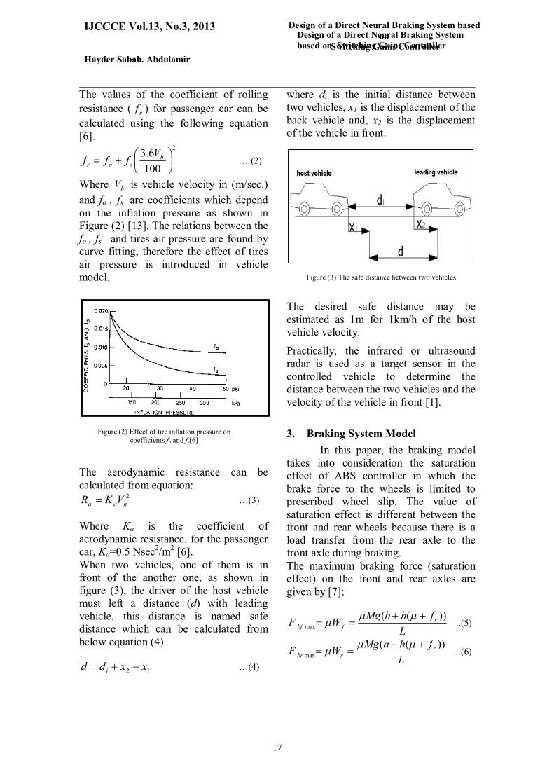
shown in figure (10) and the distance between the vehicles become 24.8m as shown in figure (11), this is an acceptable safe distance. Also the case-1 is implemented when the road is wet and the controller gives an acceptable performance as shown in figures (10) and (11). The distance is 22m and this larger than the recommended distance of 20m. The SGC gives the distances of 15.4 and 12.8 meter on the dry and wet road respectively. Case-2 In this case the difference between the velocities of vehicles is very large and the initial separation distance is small. The host vehicle and the vehicle in front are traveling in 90km/h and 10 km/h respectively on dry and wet road. The initial distance between them is 50 m which is less than the safe distance of 90m. 10 km/h at 2.5 second as shown in figure (12) and the distance between the vehicles become 22 m, figure (13). While





_____________________________________________________________________________________

23

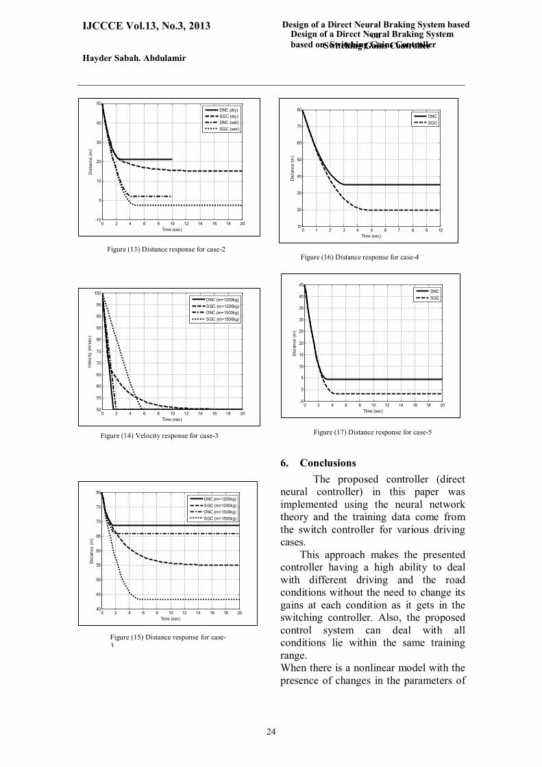
for the wet road, the distance of 15m is still larger than the recommended distance of (10m). It can be seen that the SGC fails to prevent the crashing of the vehicles at wet road condition. Case-3 This case tests the performance of DNC when the mass of vehicle is changing. The initial conditions are: the velocity of host vehicle is 100km/h, velocity of the vehicle in front is 50km/h and the separation distance is 80m. The responses of the velocity and the distance are shown in figures (14) and (15) respectively when the mass is 1200kg and 1500kg. From these figures; we can see the DNC achieved the safe distance and velocity with respect to the results of SGC. These results mean that the performance of DNC is more robust when the parameters of the vehicle changed. The common cases that may be faced the host vehicle during drive when the leading vehicle reduces its velocity are shown in Cases 4 and 5. Case-4, the leading vehicle reduces its velocity from 45 to 40 km/h at constant deceleration of 2 m/s2. The velocity of the host vehicle is 140 km/h and the initial distance is 80m. Two controllers are succeeded to prevent the crash but the DNC which gives longer safe distance than the distance that generated from SGC, as shown in figure (16). Case-5, in this case, the velocity of the leading vehicle is reduced to zero (stop condition) at constant deceleration of 4 m/s2. The host vehicle velocity is 100 km/h and the initial distance 45m which is considered minimum safe distance to achieve the stopping in this driving condition. From figure (17), it can be seen that DNC is successful to stop the

host vehicle at 4.8 meter, while SGC fail to stop the vehicle. This case is one of the most difficult cases that may be faced the controller.

0 1 2 3 4 5 6 7 8 9 1020

25

30

35

40

45

50

Time (sec)

Vel

ocity

(m/s

ec)

DNC (dry)SGC (dry)DNC (wet)SGC (wet)

Figure (10) Velocity response for case-1

0 1 2 3 4 5 6 7 8 9 1012

14

16

18

20

22

24

26

28

30

Time (sec)

Dis

tanc

e (m

)


Figure (11) Distance response for case-1


0 2 4 6 8 10 12 14 16 18 200

10

20

30

40

50

60

70

80

90

Time (sec)

Vel

ocity

(m/s

ec)






_____________________________________________________________________________________

24

6. Conclusions

The proposed controller (direct neural controller) in this paper was implemented using the neural network theory and the training data come from the switch controller for various driving cases.

This approach makes the presented controller having a high ability to deal with different driving and the road conditions without the need to change its gains at each condition as it gets in the switching controller. Also, the proposed control system can deal with all conditions lie within the same training range. When there is a nonlinear model with the presence of changes in the parameters of

0 2 4 6 8 10 12 14 16 18 2050

55

60

65

70

75

80

85

90

95

100

Time (sec)

Vel

ocity

(m/s

ec)

DNC (m=1200kg)SGC (m=1200kg)DNC (m=1500kg)SGC (m=1500kg)


0 2 4 6 8 10 12 14 16 18 20-10

0

10

20

30

40

50

Time (sec)

Dis

tanc

e (m

)



0 2 4 6 8 10 12 14 16 18 2040

45

50

55

60

65

70

75

80

Time (sec)

Dis

tanc

e (m

)

DNC (m=1200kg)SGC (m=1200kg)DNC (m=1500kg)SGC (m=1500kg)


0 1 2 3 4 5 6 7 8 9 1010

20

30

40

50

60

70

80

Time (sec)

Dis

tanc

e (m

)

DNCSGC


0 2 4 6 8 10 12 14 16 18 20-5

0

5

10

15

20

25

30

35

40

45

Time (sec)

Dis

tanc

e (m

)

DNCSGC






_____________________________________________________________________________________

25

the system, the use of control systems is preferred like the proposed controller in this research. Because of the presence of the intrinsic characteristics of neural network in having internal memory, they are capable of modeling nonlinear dynamic system. Direct neural controller is tested with a nonlinear braking vehicle model. The results give acceptable responses for velocity and safe distance for different cases even in difficult cases in comparison with the switching controller results.

References [1] Hsien-Ping Chu and Bo-Rong Liang “ Neural-

Network Synthesis of Integrated Brake Controller of Electrical Vehicle” 5th IEEE Conference on Industrial Electronics and Applications, 2010.

[2] M. Chadli, A. El Hajjaji, A. Rabhi “H∞ Observer-based robust multiple controller design for vehicle lateral dynamics” 2010 American Control Conference Marriott Waterfront, Baltimore, MD, USA June 30-July 02, 2010

[3] Chih-Min Lin and Chun-Fei Hsu “Neural-Network Hybrid Control for Antilock Braking Systems” IEEE TRANSACTIONS ON NEURAL NETWORKS, Vol. 14, NO. 2, MARCH 2003.

[4] Chunting Mi, Hui Lin, and Yi Zhang “Iterative Learning Control of Antilock Braking of Electric and Hybrid Vehicles” IEEE TRANSACTIONS ON VEHICULAR TECHNOLOGY, Vol. 54, No. 2, March 2005

[5] Li Guo and Peng Sha” Research on the Steering Antilock Braking Control System for the Vehicles” 2011 International Conference on Mechatronic Science, Electric Engineering and Computer August 19-22, 2011, Jilin, China

[6] Jian Zhao and Litong Guo “Modeling and control of automotive antilock brake systems through PI and neural network arithmetic ” Electronic and Mechanical Engineering and Information Technology (EMEIT), International Conference, 2011.

[7] Merry Cherian and S.Paul Sathiyan “ Neural Network based ACC for Optimized Safety and Comfort” International Journal of Computer Applications) Vol. 42– No.14, March 2012.

[8] Felipe C. and Alexis A.” Design and Validation of a Fuzzy Longitudinal Controller Based on a Vehicle Dynamic Simulator” 2011 9th IEEE International Conference on Control and Automation (ICCA) Santiago, Chile, December 19-21, 2011.

[9] Atilla K. and Huseyin B “Determination of brake force using artificial neural network “Journal of scientific and industrial research , Iterative Learning Control of Antilock Braking of Electric and Hybrid VehiclesVol.66, pp.425-430,June 2007

[10] Meihua Tai and Masayoshi Tomizuka" Robust Longitudinal Velocity Tracking of Vehicles Using Traction and Brake Control" IEEE ,2000.

[11] Mike Bauer and Masayoshi Tomizuka "fuzzy logic traction controllers and their effect on longitudinal vehicle platoon system", vehicle system dynamics,Vol.25.1996.

[12] Reza Jafari "Adaptive PID controller for a nonlinear pendulum system using recurrent neural networks" M.SC. Faculty of the American University of Sharjah, School of Engineering, 2005.

[13] Wong .J yong. "Theory of ground vehicle. 'John willy &Sons,Inc.,1993

[14] K. R. Buckholtz “ Use of fuzzy logic in wheel slip assignment-part I: yaw rate control” SAE 2002 world congress. March 4-7,2002.

[15] David W. Spitzer " Advanced Regulatory Control: Applications and Techniques", Momentum Press, 2009.

[16] Pham D. T. and Xing L. " Neural Networks for Identification, Prediction and Control", Springer, 1995.

[17] S. Omatu, M. Khalid, and R. Yusof "Neuro-Control and its Applications" London: Springer-Velag, 1995. Nomenclatures

a=length from mass center to front axle (m) ah= deceleration (m/sec2) b=length from mass center to rear axle (m) d= distance between two vehicles (m) di= initial distance between two vehicles(m) ed=distance error (m) ev=relative velocity error (m/sec) E= cost function

bfF=front brake force (N)

brF =rear brake force (N) FNb=neural network brake force (N)

rf = coefficient of rolling resistance.





_____________________________________________________________________________________

26

fo, fs = coefficients depend on the inflation pressure.

g=acceleration of gravity (m/sec2) H= nonlinear node with sigmoidal function h=height of the center of mass (m) L=vehicle track (m) and linear node. Ka= coefficient of the aerodynamic resistance

(Nsec2/m2) Kbf, Kbr = ratio of the total braking force on the

front and rear axles K1,K2=gain of switching controller M=vehicle mass (kg) m= index of time o= outputs of output layer Ra=aerodynamic resistance (N) Uji= Weight of first hidden layer Ubi=bias weight for first hidden layer Vkj= Weight of second hidden layer Vbj=bias weight for second hidden layer Vh=host vehicle velocity (m/sec.) Wlk= Weight of output layer Wbk=bias weight for output layer Wf=normal load on the front axle (N) Wr= normal load on the rear axle (N) x1= displacement of the back vehicle(m) x2= displacement of the vehicle in front (m) =angle of the slop with the horizontal (deg) µ= coefficient of road adhesion = outputs of first hidden layer = learning rate = outputs of second hidden layer

Appendix –A Physical parameters of the vehicle m=1200kg L=2.5 m a=1 m b=1.5m

Ka=0.5 Nsec2/m2 h=0.6m µ=0.9 for dry road, 0.5 for wet road

Appendix –B Neural network weights U=[ 0.1389 0.9080 -0.1592 -0.7203 0.6975

1.2602 -0.6295 0.1989 0.4057 0.1117 -0.6289 -

0.8398 -1.4113 -0.1211 -0.4647 -0.5102 -0.0237

0.5721 0.5239 0.1759 0.6346 0.5791 -1.4004 -

0.4002 1.6552 -0.4451 -0.6373 0.8688 0.3752

0.8947 -0.1570 0.4076 0.2630 -1.2988 -1.3316

0.5231

0.5576 1.0042 0.9396 -0.9900 1.1537 0.0424

-0.3794 0.4940 2.1834 0.0830 0.2939 -0.2959

1.6590 -0.1583 -0.9977 -0.4214 0.3472 0.6934

-1.4836 0.0754 -0.7593 0.3737 0.8640 0.6736

-0.6040 -1.2771 -0.8120 0.2403 -0.7598 -0.3224

0.8256 0.7268 -0.4658 -0.9538 0.1284 -0.6531]

Ub=[ -2.1853 1.7755 2.6886 -1.4210 0.3850 -

0.0245 0.5018 -0.6261 1.3673 -1.1524 0.5543 1.9463]T

V=[ 1.012 -0.899 -1.018 0.231 -0.007 0.098 0.985 0.395 0.663 -0.502 -0.165 -0.1563

0.5885 1.1695 0.5242 0.6710 0.780 -0.0055 0.8612 0.7082 1.5435 1.4407 1.4281 -0.7501

-0.3918 -0.5886 0.2133 -0.4089 0.8634 0.3527 0.8293 0.5480 1.0266 -0.1318 -0.2118 0.5631

-0.0936 -0.8699 0.4844 -0.2536 0.8130 0.1091 0.2972 0.1883 1.1175 -0.7918 -0.6890 0.1793

-0.8136 -0.3899 1.2831 0.1137 -0.2354 0.5851 0.4314 0.7297 0.1130 -0.0911 0.9052 -0.6161

-0.3236 0.8228 0.0390 0.8019 -1.2915 1.3540 0.5329 -0.0599 -2.2487 -0.6940 -1.0102 -0.0079

-0.3817 0.3686 -1.4307 0.6251 -0.1923 -0.2680 0.0610 1.0088 1.0625 0.3563 -0.9838 0.4939

-0.5170 0.2385 0.0868 -0.5453 -1.0841 -1.0603 -0.5745 0.7051 -0.2930 -0.6314 -0.9974 0.2727

-0.5261 1.0174 0.5933 -0.0085 0.1454 -0.4957 -0.5302 0.2814 -2.1127 0.8037 -0.1832 -0.4509

-0.6287 0.3891 -0.9206 0.1499 -0.1708 0.1850 -0.4551 -0.5868 -0.0546 0.1380 -1.2542 -0.3001

-0.7531 -0.8381 -0.1040 -0.7869 -0.5756 -0.0892 -0.8384 -0.2025 0.2762 0.1120 -0.1131 0.3710

0.6719 0.4046 1.4512 0.0535 0.1495 -0.0311 -0.5548 -0.8030 0.6168 0.6103 -0.0486 0.5933 ]

Vb=[ -1.7461 -0.7488 0.7074 1.0785 0.6076

0.2491 0.0406 -0.6163 -0.6243 -1.7292 -1.4636 0.2342]T

W=[ 2.0489 1.6416 0.8354 1.0331 -0.7401 -0.2857 1.1733 0.0253 -1.7252 0.0827 -0.2391 -1.4594]

Wb= [ -0.8904]

design of a direct neural braking system based on

Documents