Design of a controlled-forcegrinder for free-form lenses

M.A.J.Ras

DCT 2006.17

Master’s thesis

Coach(es): dr. ir. P. C. J. N. Rosielle, TU/edr. ir. H. van Brug, TNO Science and Industry

Supervisor: prof. dr. ir. M. Steinbuch, TU/e

Technische Universiteit EindhovenDepartment Mechanical EngineeringDynamics and Control Technology Group

Eindhoven, February, 2006

Summary

One of the research areas of the Opto-Mechanical Instruments department within TNO Science andIndustry is the fabrication of optical components for scientific and industrial applications. The over-all goal is to improve all steps in the manufacturing process that consists of grinding, polishing andmeasuring. Most of the research is focussed on the production of single piece free-form optics. Thepolishing research is conducted with the fluid jet polisher, FJP, on which Silvia Booij wrote her disser-tation [Boo03]. Rens Henselmans, [Hen05], is currently working on the design of the NANOMEFOS,which will be able to optically measure unique free-form optics with an accuracy of 30 nm.

This thesis will describe an improvement of the grinding process using controlled-force grinding.When controlling the force applied by the grinding tool onto a brittle workpiece, such as glass, it ispossible to machine it in a ductile way. Brittle ground optical components contain subsurface damage,which are cracks reaching several µm’s inside the material. The polishing process to remove thesecracks is very time consuming and requires an iterative process of polishing and measuring in orderto get a good shape accuracy. The grinder of this thesis features a controlled-force tool spindle thatis able to limit the amount of force it applies on the workpiece. It will be able to produce opticalcomponents with high shape accuracy and a very low amount of subsurface damage. The design ofthe controlled-force tool spindle is emphasized, so this spindle can be build shortly after completingthis thesis and can be used in an experimental setup to investigate the potential of controlled-forcegrinding on a brittle workpiece.

2

Contents

Summary 2

1 Introduction 6

2 Goals and conditions 82.1 Main goals . . . . . . . . . . . . . . . . . . . . . . . . . . . . . . . . . . . . . . . . . . 82.2 Other conditions . . . . . . . . . . . . . . . . . . . . . . . . . . . . . . . . . . . . . . . 9

3 Grinding of optical components 103.1 Introduction . . . . . . . . . . . . . . . . . . . . . . . . . . . . . . . . . . . . . . . . . 103.2 Fundamentals of grinding . . . . . . . . . . . . . . . . . . . . . . . . . . . . . . . . . . 103.3 Trueing, dressing, conditioning . . . . . . . . . . . . . . . . . . . . . . . . . . . . . . . 113.4 Grinding methods . . . . . . . . . . . . . . . . . . . . . . . . . . . . . . . . . . . . . . 12

3.4.1 Position-controlled precision grinding . . . . . . . . . . . . . . . . . . . . . . . 123.4.2 Precitech slow tool grinder . . . . . . . . . . . . . . . . . . . . . . . . . . . . . 133.4.3 Controlled-force internal grinding . . . . . . . . . . . . . . . . . . . . . . . . . 133.4.4 FAUST . . . . . . . . . . . . . . . . . . . . . . . . . . . . . . . . . . . . . . . . 143.4.5 WAGNER . . . . . . . . . . . . . . . . . . . . . . . . . . . . . . . . . . . . . . 14

3.5 Subsurface damage . . . . . . . . . . . . . . . . . . . . . . . . . . . . . . . . . . . . . 153.5.1 Creation . . . . . . . . . . . . . . . . . . . . . . . . . . . . . . . . . . . . . . . 153.5.2 Detection . . . . . . . . . . . . . . . . . . . . . . . . . . . . . . . . . . . . . . . 163.5.3 Determining the grinding force . . . . . . . . . . . . . . . . . . . . . . . . . . 16

4 Machine concepts and layouts 194.1 Introduction . . . . . . . . . . . . . . . . . . . . . . . . . . . . . . . . . . . . . . . . . 194.2 Unstacked machine concept . . . . . . . . . . . . . . . . . . . . . . . . . . . . . . . . . 194.3 Machine layout . . . . . . . . . . . . . . . . . . . . . . . . . . . . . . . . . . . . . . . . 19

4.3.1 Introduction . . . . . . . . . . . . . . . . . . . . . . . . . . . . . . . . . . . . . 194.3.2 Layout 1, T-configurations . . . . . . . . . . . . . . . . . . . . . . . . . . . . . . 204.3.3 Layout 2, fixed workpiece spindle, large y-slide . . . . . . . . . . . . . . . . . . 204.3.4 Layout 3, fixed workpiece spindle, small y-slide . . . . . . . . . . . . . . . . . . 204.3.5 Orientation of the machine layout . . . . . . . . . . . . . . . . . . . . . . . . . 21

4.4 Measurement loop . . . . . . . . . . . . . . . . . . . . . . . . . . . . . . . . . . . . . . 224.5 Conclusion . . . . . . . . . . . . . . . . . . . . . . . . . . . . . . . . . . . . . . . . . . 24

5 Tool spindle concepts 255.1 Introduction . . . . . . . . . . . . . . . . . . . . . . . . . . . . . . . . . . . . . . . . . 255.2 Controlled-force grinding spindle . . . . . . . . . . . . . . . . . . . . . . . . . . . . . . 255.3 Concept 1, using an elastic guideway . . . . . . . . . . . . . . . . . . . . . . . . . . . . 255.4 Concept 2, using an aerostatic guideway . . . . . . . . . . . . . . . . . . . . . . . . . . 265.5 Comparing spindle concepts . . . . . . . . . . . . . . . . . . . . . . . . . . . . . . . . 275.6 Tool drive measurement . . . . . . . . . . . . . . . . . . . . . . . . . . . . . . . . . . . 275.7 Sealing . . . . . . . . . . . . . . . . . . . . . . . . . . . . . . . . . . . . . . . . . . . . 28

3

6 Machine design 306.1 Introduction . . . . . . . . . . . . . . . . . . . . . . . . . . . . . . . . . . . . . . . . . 306.2 Machine design overview . . . . . . . . . . . . . . . . . . . . . . . . . . . . . . . . . . 306.3 Tool drive . . . . . . . . . . . . . . . . . . . . . . . . . . . . . . . . . . . . . . . . . . . 30

6.3.1 Tool drive assembly . . . . . . . . . . . . . . . . . . . . . . . . . . . . . . . . . 306.3.2 Tool drive components . . . . . . . . . . . . . . . . . . . . . . . . . . . . . . . 32

6.4 Tool spindle . . . . . . . . . . . . . . . . . . . . . . . . . . . . . . . . . . . . . . . . . . 346.4.1 Spindle assembly . . . . . . . . . . . . . . . . . . . . . . . . . . . . . . . . . . 346.4.2 Tool spindle components . . . . . . . . . . . . . . . . . . . . . . . . . . . . . . 356.4.3 Motor stator . . . . . . . . . . . . . . . . . . . . . . . . . . . . . . . . . . . . . 386.4.4 Toolholder front . . . . . . . . . . . . . . . . . . . . . . . . . . . . . . . . . . . 386.4.5 Toolholder back . . . . . . . . . . . . . . . . . . . . . . . . . . . . . . . . . . . 40

6.5 Tool disk . . . . . . . . . . . . . . . . . . . . . . . . . . . . . . . . . . . . . . . . . . . 406.5.1 Tool disk assembly . . . . . . . . . . . . . . . . . . . . . . . . . . . . . . . . . . 406.5.2 Tool disk components . . . . . . . . . . . . . . . . . . . . . . . . . . . . . . . . 40

6.6 Y-slide . . . . . . . . . . . . . . . . . . . . . . . . . . . . . . . . . . . . . . . . . . . . . 416.6.1 Y-slide assembly . . . . . . . . . . . . . . . . . . . . . . . . . . . . . . . . . . . 416.6.2 Y-slide components . . . . . . . . . . . . . . . . . . . . . . . . . . . . . . . . . 42

6.7 X-slide . . . . . . . . . . . . . . . . . . . . . . . . . . . . . . . . . . . . . . . . . . . . . 446.7.1 X-slide assembly . . . . . . . . . . . . . . . . . . . . . . . . . . . . . . . . . . . 446.7.2 X-slide components . . . . . . . . . . . . . . . . . . . . . . . . . . . . . . . . . 44

6.8 Base . . . . . . . . . . . . . . . . . . . . . . . . . . . . . . . . . . . . . . . . . . . . . . 486.8.1 Base assembly . . . . . . . . . . . . . . . . . . . . . . . . . . . . . . . . . . . . 486.8.2 Base components . . . . . . . . . . . . . . . . . . . . . . . . . . . . . . . . . . 49

7 Conclusions and recommendations 527.1 Conclusions . . . . . . . . . . . . . . . . . . . . . . . . . . . . . . . . . . . . . . . . . 527.2 Recommendations . . . . . . . . . . . . . . . . . . . . . . . . . . . . . . . . . . . . . . 52

Bibliography 54

Symbol list 57

A Assembly drawings 58

B Summary machine properties 62

C Tool spindle cost 63

D Dynamical model 64

E FEM-calculations 67E.1 Introduction . . . . . . . . . . . . . . . . . . . . . . . . . . . . . . . . . . . . . . . . . 67E.2 X-frame . . . . . . . . . . . . . . . . . . . . . . . . . . . . . . . . . . . . . . . . . . . . 67E.3 Vacuum seal . . . . . . . . . . . . . . . . . . . . . . . . . . . . . . . . . . . . . . . . . 67E.4 Membranes . . . . . . . . . . . . . . . . . . . . . . . . . . . . . . . . . . . . . . . . . . 70E.5 X-frame airbearings . . . . . . . . . . . . . . . . . . . . . . . . . . . . . . . . . . . . . 70

F Calculations 72F.1 Stiffness related to overhanging length . . . . . . . . . . . . . . . . . . . . . . . . . . . 72F.2 Tool spindle accuracy model . . . . . . . . . . . . . . . . . . . . . . . . . . . . . . . . . 72

4

G Alternative machine designs 76G.1 Alternative 1 . . . . . . . . . . . . . . . . . . . . . . . . . . . . . . . . . . . . . . . . . 76G.2 Alternative 2 . . . . . . . . . . . . . . . . . . . . . . . . . . . . . . . . . . . . . . . . . 77G.3 Alternative 3 . . . . . . . . . . . . . . . . . . . . . . . . . . . . . . . . . . . . . . . . . 79G.4 Alternative spindle design . . . . . . . . . . . . . . . . . . . . . . . . . . . . . . . . . . 80

G.4.1 Alternative spindle design 1 . . . . . . . . . . . . . . . . . . . . . . . . . . . . . 80G.4.2 Alternative spindle design 2 . . . . . . . . . . . . . . . . . . . . . . . . . . . . 80

H Materials 82H.1 Optical materials . . . . . . . . . . . . . . . . . . . . . . . . . . . . . . . . . . . . . . . 82

I Data sheets 83

5

Chapter 1

Introduction

Optical components, like lenses and mirrors, are made to manipulate the propagation of light raysso they can be used to measure objects, as done with interferometry, or to manufacture products, forexample making IC’s using lithography. To achieve a good optical performance first of all a materialmust be chosen with the right physical properties. This material is then to be shaped into its desiredform. One of the ways of shaping optical components is grinding. Grinding is often used with veryhard materials, such as glass. The grinding method must provide a number of things, starting with ahigh shape accuracy to ensure a high imaging performance. Also the surface must be smooth enoughto avoid scattering and the amount of subsurface damage has to be low to avoid deterioration if thelens is used with high power laser beams, [Fäh99].

There is an increasing demand for free-form shaped lenses. An aspherical lens for example canavoid geometrical aberrations and this will reduce the number of lenses needed for an application,thus reducing the number of optical surfaces and absorption. This way the required space inside anapplication is also reduced. The processes to polish and measure free-form lenses are currently beingdeveloped, [Boo03],[Hen05].

Subsurface damage arises when the grinding process takes place in brittle mode, see chapter 3.The problem with this kind of damage is that it is possible for chips to break out of the lens when it isbeing used, reducing its quality significantly. The damage also increases the amount of light absorbedby the lens, causing the lens to heat up which is undesirable for a lot of applications. The lens ispolished to remove the subsurface damage, but this will decrease the shape accuracy, because mostpolishing processes have an averaging effect on the surface form. This also is a very time-consumingprocess with repeatedly polishing and measuring.

Grinding glass into free-forms without leaving subsurface damage using position-controlled ma-chines is very challenging with currently available machines, because it requires a depth of cut smallerthan one tenth of a micrometer. Because of machine vibrations and height variations of the roughlyground workpiece, even if the infeed is set small enough, the critical depth of cut is often exceeded.Another problem is wear of the abrasive grains. Sharp grains can cut away material of the workpiecewith a very small normal force pressing them into the workpiece. When the grains dull, they tend torub more and cut less, so a larger normal force is necessary to achieve the desired depth of cut. Whenthe normal force reaches a value that is larger than the force correlated to the critical depth of cut,brittle fracture and subsurface damage occur.

This thesis will discuss the design of a grinding machine that uses a controlled-force grindingmethod. The force at which subsurface damaged arises is, depending on the tool used, around 1 N.By on one hand positioning the tool accurately and on the other hand ensuring the normal force onthe workpiece never exceeds 1 N, it should be possible to produce an accurately shaped lens withoutsubsurface damages. The machine accuracy is necessary only for the shape accuracy of the workpiece,

6

not for limiting the grinding force. This way a larger machine error can be allowed, this will not leadto subsurface damage.

At the locations where the force would be larger than 1 N if position-controlled grinding was ap-plied, the shape will differ from the desired shape. This is shown in figure 1.1. In previous grindingsteps the workpiece surface was ground into the shape as shown with the dotted line. A depth of cut,dset, is set to reach the final shape given by the straight dashed line. However, because dset is largerthan the critical depth of cut dcrit related to the maximum allowable grinding force, the desired shapeis not achieved in one step. A lump still remains on the left part of the figure. Most of the right partof the figure did reach its final shape. If this lump is small enough, so the desired shape accuracy isachieved, the grinding process is complete. Else an extra step is necessary.

d c r i t d s e t

Figure 1.1: Controlled force toolpath

7

Chapter 2

Goals and conditions

2.1 Main goals

Controlled force

The primary objective of this grinder is to control the force applied by the tool onto the workpiece. Thiscan be done by controlling the position of the tool relative to the workpiece very accurately, but this isvery difficult, because a depth of cut of about 10 nm is necessary. There have been done experimentswith a position-controlled grinder grinding in ductile mode, [Bif91], but this has only been applied onflat workpieces, not with free-form ones.

Because controlling the grinding force is difficult with a position-controlled grinder, a design willhave to be made that will allow the grinding force to be set. This way the position of the tool and thegrinding force are no longer related. The tool is positioned to a desired depth of cut and the tool tipcan vary somewhat in position so the force on the tool tip can be lower than the set maximum. Theworkpiece can push the tool away, to avoid the grinding force to become too large. If the positionvariation of the tool tip is so large that the shape accuracy is not achieved, another grinding pass isneeded. Extra time is then needed to grind the workpiece, but it does not suffer from subsurfacedamage.

Free-form surfaces

Free-form optical components can have many advantages compared to rotational-symmetric compo-nents. They allow light to be manipulated using less optical surfaces. The grinder must be able togrind such surfaces. Because many lenses are (almost) rotational-symmetric, even the free-form ones,a machine layout has to be chosen that is best suited for this kind of workpieces. This grinder can beless suited for entirely non-rotational-symmetric components such as cubes and prisms.

Shape accuracy

Currently a maximal accuracy of 1 µm is achieved, when grinding rotational-symmetric lenses. Exper-iments on grinding free-form lenses with a grinder built for rotation-symmetric lenses resulted in farless accurate workpieces. The goal for this machine is to produce lenses with an error less than 1 µm.This means that the produced axis of rotation of the workpiece should not be more than 1 µm awayfrom the desired axis of rotation. Also the height variations should be less than 1 µm.

Tool spindle unit

There are plans to first build the tool spindle and use it on an existing platform, e.g. a milling machine.This way experiments can be done to analyze the potential of controlled-force grinding. Therefor the

8

tool spindle should be designed as a stand-alone unit that can be placed onto a platform as a whole. Toget a good shape accuracy during these experiments, the position of the tool relative to the tool spindlehousing should be measured with 0.2 µm accuracy.

2.2 Other conditions

Most glass lenses that are currently being produced have a diameter of less than 200 mm. Thereforthis diameter was set as the maximum diameter for the grinder. Because this grinder will be usedfor experiments to examine the possibility of controlled-force grinding, a high production rate is notan important issue. It must show the potential of controlled-force grinding. To optimally controlthe grinding process it is important to have a stable grinder with a good dynamical behaviour. Thismeans material has to be used in an optimal way, resulting in stiff machine components with a limitedweight. Critical components are to be statically determined.

9

Chapter 3

Grinding of optical components

3.1 Introduction

In this chapter the basics of grinding are explained. First is examined how forces act on an individualabrasive grain, then the forces on the entire grinding tool are shown. To get a tool that has a definedgeometry with sharp grain, it needs to be trued and dressed. Further a number of grinding methodsare discussed, to give the reader an overview of the different grinding processes. Finally the creationand detection of subsurface damage is discussed.

3.2 Fundamentals of grinding

Like all classes of machining, grinding is used to remove unwanted material from the workpiece[Heg00]. An abrasive surface is pressed against the workpiece and by mechanical action of the abra-sive grains, material is removed, shown in figure 3.1. A grain is moved into the workpiece with toolspeed vt. A normal force Fn pushes the grain into the workpiece, while the cutting force Fc removesmaterial. Usually diamonds bonded in bronze are used for grinding glass. For the design in thisthesis a cup wheel is chosen, because it can be used to grind small concave areas, shown in figure 3.2.The normal grinding force in these wheels can be almost perfectly axial, which is best suited for theconcept used, described in chapter 5. Fc is pointing into the paper. The angle α is best kept low toreduce the influence of roundness errors and to minimize bending of the tool.

F n

F c v t

Figure 3.1: Forces on cutting grain

When an abrasive grain comes into contact with the workpiece, there are four different deforma-tion mechanisms that can occur, providing the grain is not pulled from its bond. Figure 3.3 showsthese four mechanisms. Ploughing (a) occurs when a grain is not sharp enough or is not deep enough

10

vw

Fn

Fc α

Figure 3.2: Forces on cutting cupwheel

into the workpiece to remove material. Instead material in front of the grain is pushed forward andsideward. This way a scratch is made, but no material is removed. Ideally the grains are cuttingmaterial from the workpiece and the surrounding material is unmoved (b). As a result of repeatedploughing micro-fatigue may take place (c). Finally when grinding brittle material, like glass in brittlemode, cracking can occur (d). Material from an area larger that the cutting area of the abrasive grain isremoved. This leaves a rough surface and subsurface damage. Cracking is the only brittle deformationmechanism, so the other three are to be expected when grinding glass in ductile mode.

3.3 Trueing, dressing, conditioning

To achieve a ground product with a good form and finish it is necessary to true and dress the grindingwheel regularly, [Sha96]. In most cases the manufacturer of the wheel has balanced it, but for thistype of grinding it will be needed to balance the wheel in the machine. This way the misalignment tothe axis of rotation of the tool spindle, due to the mounting of the tool, can be compensated.The process of removing material from the grinding surface of the tool and giving it a defined shape iscalled truing. This way the runout will be decreased. However it also flattens some of the outer grainsin order to reach the defined geometry. After truing the tool needs to be sharpened.The process to sharpen the active grids by removing wear flats and the bondmaterial is called dressing.Finally conditioning is used to open up spaces between the active grid so chips can be accommodated.For super abrasive wheel this is mostly done by plunging an Al2O3 abrasive stick into the wheel andthis way scratching out the softer bond material between the abrasive grid.Currently grinders are being designed that are able to continuously dress their tools while grinding,[Qia04]. This ELectrolytic In-process Dressing, ELID, uses electric current to erode the bond materialfrom the tool in a controlled way. This way dull grains are removed and the tool stays in optimalgrinding condition.Because ELID grinding is a complex process, that still needs research to get the desired results, it is nottaken into account in this thesis. The major new feature of this grinder is controlled-force grinding.

11

Figure 3.3: a) ploughing, b) cutting, c) fatigue, d) cracking

3.4 Grinding methods

3.4.1 Position-controlled precision grinding

One way to avoid subsurface damage is to build a high precision grinder and by using a very smallinfeed limiting the grinding forces. This requires a very stiff machine which drives must be able tobe positioned very accurately. [Bif91] built an experimental setup (PEGASUS) for ductile grinding byplacing the tool spindle onto an elastic guideway. The infeed is controlled by a piezoelectric actuatorwith a resolution of 2 nm over a range of 10 µm. Using PEGASUS it was possible to plunge grindfused silica with an infeed of 2 nm per revolution leaving a ductile cut surface. This illustrates thesmall infeed needed to grind in ductile mode. When plunge grinding the tool wheel used is muchlarger than the workpiece. This way no radial movement is necessary to make flat workpieces.

Figure 3.4: Position controlled grinding with Pegasus

Expansion of machine components by an increase in temperature causes position errors if not

12

properly dealt with. For the design of a grinder to grind flat optical and electronic parts, [Nam89] useda Zerodur tool spindle. Zerodure is a glass with a very small thermal expansion coefficient. Despitethe low modulus of elasticity compared to steel, a flatness of 0.2 µm is achieved on an area of 18 x 18mm.

The two processes described above are capable of grinding only flat surfaces. A grinder for themanufacturing of aspheric mirrors with maximal dimensions of 500 mm x 500 mm was designed by[Suz95]. To reduce the influence of vibrations from the tool spindel motor on the workpiece, a viscouscoupling between this motor and the grinding wheel spindle was designed. The slides are driven byball screws, which are mounted to the slides with flexible couplings, so only thrust is applied. This isnecessary to avoid an overconstrained slide position and gain good accuracy, [Sch98]

Another precision position-controlled grinder is designed by [Qia04], this project is called Nanogrind. The grinder is a high precision 5-axis machine integrated with ELID technology. This ’Elec-trolytic In-process Dressing’ makes it possible to continuously keep the tool in optimal cutting con-dition, by eroding the bonding material in a controlled way, so dull grains can be pulled out by theworkpiece. This way the grinding force is mostly prescribed by sharp grains, so the grinding force iskept at a low value. This design also features an in-situ measurement device, so the position of thetool and workpiece can directly be measured .

3.4.2 Precitech slow tool grinder

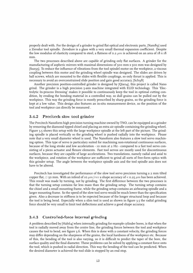
The Precitech Nanoform high precision turningmachine owned by TNO, can be equipped as a grinderby removing the diamond tipped chisel and placing an extra air spindle containing the grinding wheel.Figure 3.5 shows this setup with the large workpiece spindle at the left part of the picture. The grind-ing spindle is placed vertically so the grinding wheel is pushed radially into the workpiece. Pleasenote that a very small diameter wheel is used. The Nanoform also features a slow tool servo machin-ing option. This type of servo is particulary suited for machining non-rotational continuous surfaces,because of the long stroke and low acceleration - 10 mm at 2 Hz - compared to a fast tool servo con-sisting of a piezo actuator and flexure elements. Fast tool servos are mostly used for discontinuoussurfaces, because they are capable of large accelerations. Two translations, namely radial and axial tothe workpiece, and rotation of the workpiece are sufficient to grind all sorts of free-form optics withthis grinder setup. The angle between the workpiece spindle axis and the tool spindle axis does nothave to be altered.

Precitech has investigated the performance of the slow tool servo precision turning a 2 mm tiltedcopper flat, � 50 mm. With an infeed of 10 µm/rev a shape accuracy of < 0.25 µm has been achieved.This result was made by turning, not by grinding. The first difference between the two processes isthat the turning setup contains far less mass than the grinding setup. The turning setup containsthe chisel and a small mounting frame, while the grinding setup contains an airbearing spindle and alarger mounting frame. So the speed of the slow tool servo would be much lower than the specificationgiven. Also a decrease in stiffness is to be expected because of the longer structural loop and becausethe tool is being bend. Especially when a slim tool is used as shown in figure 3.5 the radial grindingforce should be very small to limit tool deflections and achieve a good shape accuracy.

3.4.3 Controlled-force internal grinding

A problem described by [Hah64] when internally grinding for example cylinder bores, is that when thetool is radially moved away from the centre line, the grinding forces between the tool and workpiececauses the tool to bend, see figure 3.6. When this is done with a constant velocity, the grinding forcesmay differ depending on the sharpness of the grains, the local hardness of the workpiece etc. Becauseof this, the bending of the tool is also varying, so it is difficult to predict the taper of the bore, thesurface quality and the final diameter. These problems can be solved by applying a constant force ontothe tool, which is pushed in radial direction. This way the bending of the tool can be predicted. Whenthe desired diameter is achieved the tool slide is stopped by an end stop.

13

Figure 3.5: Precitechs aspheric grinding setup

V

Figure 3.6: De�ection by uncontrolled grinding force with constant tool speed V

3.4.4 FAUST

Oliver W. Fähnle, [Fäh98], describes in his dissertation the fabrication technique ’Fabrication of As-pherical Ultra-precise Surfaces using a Tube (FAUST). This methode uses the edge of an ellipticallyshaped tube to grind parabolic and hyperbolic surfaces. Figure 3.7 shows the tool T having an angle αwith workpiece W . By choosing the right rotational speeds of the workpiece ω1 and the tool ω2, after acertain time all the grinding points on tube M have been in contact with the entire workpiece surface.During grinding the tool will be moved into −z direction until the desired shape is acquired. So onlyone degree of freedom is actuated during grinding and this is done by using a spring. This way thetool is pressing against the workpiece with a constant force until it reaches its end stop.

3.4.5 WAGNER

Amachining tool based on the same concept as FAUST is ’Wear-based Aspherics Generator based ona Novel Elliptical Rotator (WAGNER)’. This tool consists of a small diameter cup wheel that is placedon a pantograph. The pantograph describes the elliptical trajectory for the cup wheel. By choosing

14

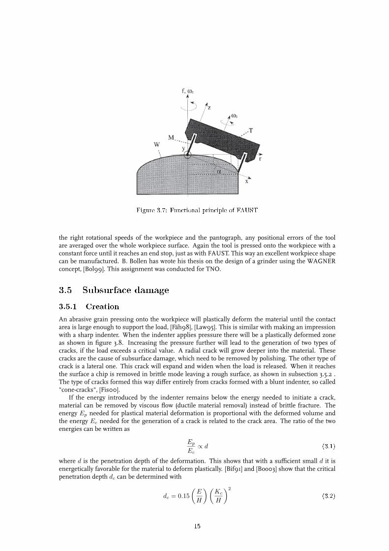
Figure 3.7: Functional principle of FAUST

the right rotational speeds of the workpiece and the pantograph, any positional errors of the toolare averaged over the whole workpiece surface. Again the tool is pressed onto the workpiece with aconstant force until it reaches an end stop, just as with FAUST. This way an excellent workpiece shapecan be manufactured. B. Bollen has wrote his thesis on the design of a grinder using the WAGNERconcept, [Bol99]. This assignment was conducted for TNO.

3.5 Subsurface damage

3.5.1 Creation

An abrasive grain pressing onto the workpiece will plastically deform the material until the contactarea is large enough to support the load, [Fäh98], [Law95]. This is similar with making an impressionwith a sharp indenter. When the indenter applies pressure there will be a plastically deformed zoneas shown in figure 3.8. Increasing the pressure further will lead to the generation of two types ofcracks, if the load exceeds a critical value. A radial crack will grow deeper into the material. Thesecracks are the cause of subsurface damage, which need to be removed by polishing. The other type ofcrack is a lateral one. This crack will expand and widen when the load is released. When it reachesthe surface a chip is removed in brittle mode leaving a rough surface, as shown in subsection 3.5.2 .The type of cracks formed this way differ entirely from cracks formed with a blunt indenter, so called"cone-cracks", [Fis00].

If the energy introduced by the indenter remains below the energy needed to initiate a crack,material can be removed by viscous flow (ductile material removal) instead of brittle fracture. Theenergy Ep needed for plastical material deformation is proportional with the deformed volume andthe energy Ec needed for the generation of a crack is related to the crack area. The ratio of the twoenergies can be written as

Ep

Ec∝ d (3.1)

where d is the penetration depth of the deformation. This shows that with a sufficient small d it isenergetically favorable for the material to deform plastically. [Bif91] and [Boo03] show that the criticalpenetration depth dc can be determined with

dc = 0.15(

E

H

) (Kc

H

)2

(3.2)

15

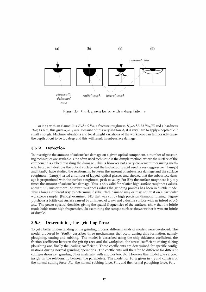
Figure 3.8: Crack generation beneath a sharp indenter

For BK7 with an E-modulus E=81 GPa, a fracture toughness Kc=0.86 MPa√

m and a hardnessH=5.2 GPa, this gives dc=64 nm. Because of this very shallow dc it is very hard to apply a depth of cutsmall enough. Machine vibrations and local height variations of the workpiece can temporarily causethe depth of cut to be too deep and this will result in subsurface damage.

3.5.2 Detection

To investigate the amount of subsurface damage on a given optical component, a number of measur-ing techniques are available. One often used technique is the dimple method, where the surface of thecomponent is etched revealing the damage. This is however not a very convenient measuring meth-ode, because it destroys the optical surface and the hydrofluoric acid used is very aggressive. [Lam97]and [Pau87] have studied the relationship between the amount of subsurface damage and the surfaceroughness. [Lam97] tested a number of lapped, optical glasses and showed that the subsurface dam-age is proportional with the surface roughness, peak-to-valley. For BK7 the surface roughness is 3 to 5times the amount of subsurface damage. This is only valid for relative high surface roughness values,about 1 µm rms or more. At lower roughness values the grinding process has been in ductile mode.This allows a different way to determine if subsurface damage may or may not exist on a particularworkpiece sample. [Fan04] examined BK7 that was cut by high precision diamond turning. Figure3.9 shows a brittle cut surface caused by an infeed of 2 µm and a ductile surface with an infeed of 0.6µm. The power spectral densities giving the spatial frequencies of the surfaces, show that the brittlemode holds more high frequencies. So examining the sample surface shows wether it was cut brittleor ductile.

3.5.3 Determining the grinding force

To get a better understanding of the grinding process, different kinds of models were developed. Themodel proposed by [You87] describes three mechanisms that occur during chip formation, namelyploughing, cutting and rubbing. The model is described using the chip thickness coefficient, thefriction coefficient between the grit tip area and the workpiece, the stress coefficient arising duringploughing and finally the loading coefficient. These coefficients are determined for specific config-urations during normal grinding operations. The coefficients will therefor be different for differentconfigurations i.e. grinding other materials, with another tool etc. However this model gives a goodinsight in the relationship between the parameters. The model for Fn is given in 3.3 and consists ofthe normal cutting force, Fnc, the normal rubbing force, Fnr, and the normal ploughing force, Fnp.

16

Figure 3.9: a)brittle mode, b)power spectral density of brittle mode, c) ductile mode, d) psd ofductile mode

Fn = Fnc + Fnr + Fnp (3.3)Fnc = wk1

vw

vgSn − La

k1vw

100vgSn (3.4)

Fnr = wLaKLlc (3.5)Fnp = wαf

vw

vglc − wLaαf

vw

vgLc) (3.6)

w width of cut [m]k1 chip thickness coe�cient [ N

mm2 ]vw speed workpiece [m/s]vg speed grinding tool [m/s]Sn Depth of cut [m]La Loaded area / Total tool area [−]KL Loading force coe�cient [ N

unitLa ]Lc Contact lenght [m]αf ploughing grain coe�cient [ N

mm2 ]

With w the width of cut. The chip thickness coefficient, k1[ Nmm2 ] gives the connection between the

chip surface and the cutting force. vw[ms ] and vg[m

s ] are respectively the speed of the workpiece andthe speed of the grinding tool. The depth of cut is given by Sn. La[−] is percentage of the total areathat is loaded, i.e. the part of the total tool surface that actually makes contact with the workpiece. La

is time dependent because initially sharp grains will flatten during grinding and thus increasing theloaded area. KL[ N

unitLa ] is the loading force coefficient, which gives the connection between the tiparea contact of the grains and the rubbing force. Lc is the contact length between grains and work-piece. Finally αf [ N

mm2 ] is the coefficient that is determined by the ploughing grain geometry. This

17

coefficient gives the relation between the surface of the ploughing grains and the required force.

The model determined by [You87] shows many parameters that depend on the workpiece and toolmaterial, grain shapes, coolant used etc. All these coefficients are best to be determined by grindingexperiments, which were not conducted during this thesis project.

Amore simplemodel is used to determine themaximum force, so the specifications of the actuatorthat will supply that force can be acquired. Figure 3.7 shows the cup wheel with angle α = 0, in thisway the contact area is as large as possible. All of the active tool area is in contact with the workpiece,not only the grain tips. Individual grains are not considered. When looking at the bottom side of thetool, one can see the contact area, which is a semi-circle band with width Lc. Because of Lc << R2,Lc is considered to be a straight line. The maximal depth of cut dmax = 1µm. The contact area Ae

can now be determined with

Ac =π

2(R1 + Lc)2 −

π

2R1

2 (3.7)

Lc =√

2R2dmax (3.8)Using [Cou04] who determined the grinding forces when machining 416 stainless steel, which

has a slightly higher hardness than glass, a grinding pressure p can be determined. The pressurewhen grinding the steel with a depth of cut of 1 µm is p = 870kPa. Using equation 3.10 a maximumgrinding force of 1.3 N is achieved.

L c d m a x

R 1

R 2

L c

R 1

A c

Figure 3.10: Maximum contact area Ac

18

Chapter 4

Machine concepts and layouts

4.1 Introduction

In this chapter different machine concepts and layouts are given. These wil describe the basic formof the grinder. Also the measurement system concept is described. In the next chapter, chapter 5, theconcepts of the machine parts are given.

4.2 Unstacked machine concept

The tool should be able to move relatively to the workpiece in radial direction (x), axial direction (y)and should be able to rotate in Rz-direction. This way free-form lenses can be produced when alsothe workpiece is rotated. The movement in x-direction is slow and with a constant speed. The move-ment in y-direction is the fast movement and is used to grind free-form features. Movement in thisdirection should be relatively fast, because a free-form feature passes the tool every rotation of theworkpiece. The y-position of the tool relative to the workpiece is dependent on the rotational positionof the workpiece. The rotation in Rz-direction is needed to orientate the tool axis nearly perpendicularto the workpiece surface. This gives a defined edge of the tool being used and reduces the influenceof the tool runout.

When the tool is placed onto a bearing on a plane, all these degrees of freedom, DOF’s, are uncon-strained while the others are not. Figure 4.1 shows the tool on its airbearing and the unconstrainedDOF’s. The tool is floating on the plane of the paper. Those other DOF’s are constrained almost di-rectly to the fixed world, i.e. the plane. Compared to a stacked layout this allows a higher stiffness andlimits the amount of errors caused by accumulated manufacturing tolerances. Because of this limitederror it is not necessary to adjust the constrained DOF’s during the machining process, there is noneed to use additional actuators and guideways.

4.3 Machine layout

4.3.1 Introduction

This section will describe a number of different machine layouts. All the layouts use the unstackedmachine concept from 4.2. The plane is provided by a block of granite. The advantages and disadvan-tages are examined and finally a choice for one of the layouts is made.

19

1. Workpiece 2. Tool

Figure 4.1: The tool spindle on a plane can move in X, Y and Rz direction

4.3.2 Layout 1, T-con�gurations

Layout 1a

This layout is a T-configuration that is also used on the Precitech Nanoform diamond turningmachine.The tool can move in y-direction and can rotate in Rz-direction. The workpiece is able to move in thex-direction. The greatest advantage here is that the two translating guideways can basically be thesame. The only differences are the direction in which they move, namely perpendicular to each other,and perhaps the dimensions of the guideway because the workpiece spindle is much heavier than thetool spindle. The movement of this heavy workpiece spindle however is its major disadvantage. Theweight of such a spindle is about 150 kg and all of this mass plus the mass of the guideway itself hasto be carried by the guideway bearings. Connecting this spindle to the fixed world will improve themachines dynamic behavior and working speed.

Layout 1b

Here the x-slide holds the tool, which can rotate in Rz inside the x-slide. The workpiece spindle cantranslate in y-direction. This layout offers the same advantages as the T-configuration of layout 1a, buthere the heavy spindle must be moved fast in the y-direction. This requires a lot of power and a verygood controller.

4.3.3 Layout 2, �xed workpiece spindle, large y-slide

In this layout the workpiece spindle is directly attached to the fixed world. By only moving the lighttool spindle, the dynamical behavior of the grinder is improved. This results in a faster machinewhich uses less power. The y-slide holds the x-slide. This will result in a large machine because thex-translation is about three times larger than the y-translation. When moving in the fast y-direction agreat amount of mass is moving, so this concept is not suited for a good dynamical performance.

4.3.4 Layout 3, �xed workpiece spindle, small y-slide

Layout 3a

This concept also has got a fixed workpiece spindle. The x-slide holds the y-slide. The tool spindle canrotate inside the y-slide. When translating in x-direction the biggest mass is moved. This is favourable

20

R z

x

y

R z

x

y

layout 1a layout 1b

Figure 4.2: layout 1, T-con�gurations

because this is the slowest moving translation, moving radially across the workpiece surface in min-utes. The mass moved by the y-slide is far less than that of the x-slide, so non-rationally symmetricfeatures can be ground fast with these features passing every rotation of the workpiece. A featurepasses the tool every few seconds.

Layout 3b

This concept also has the workpiece spindle directly connected to the fixed world. But now the y-slideis placed inside the rotating part, rotating in Ry. The main advantage here is that the centre of rotationof the tool can be put exactly onto the workpiece surface. This means a rotation of the tool will notlead to any translation. This shortens the strokes in x- and y-directions. However when the centre ofrotation is on the workpiece surface, the rotating part can only be quarter of a circle. Else it would hitthe workpiece at a given angle of the tool. Because the rotating part can only be quarter of a circle, astiff bearing connection in the direction lateral to the tool axis is very difficult.

4.3.5 Orientation of the machine layout

For each of the given layouts the choice can be made wether the plane on which the tool moves,as described in 4.2, is horizontal or vertical and if the workpiece spindle axis should be orientatedhorizontally or vertically. The vertical plane and vertical workpiece axis of figure 4.5(a) prevents theweight of the workpiece bending the workpiece spindle radially. It also features a good accessabilityfor loading and unloading workpieces. Weight compensation for the tool spindle and the y-slide arenecessary to reduce required motor capacity. Else the motor has to generate a continuous force, whichwill lead to a lot of dissipated power causing the grinder to heat up. Tool weight compensation isdependent on the angle of the tool disk, because the centre of mass of the tool spindle and disk is notin the disk centre. A vertical plane also puts the machine’s centre of mass up high, so environmentisolators should be placed carefully to have a stable isolating system.

Figure 4.5(b) also shows a vertical plane on which the tool spindle moves, but features a horizon-tally oriented workpiece spindle. Weight compensation as described for the previous orientation isstill needed. The centre of mass is still very high. Chips and grinding fluid are easily removed fromthe workpiece, even from concave ones.

Figure 4.5(c) features a horizontal plane, which brings down the centre of mass significantly. Thisdecreases the space needed for a stable isolator platform. It is safe to preload the x-slide bearings with

21

R z

x

y

Figure 4.3: Layout 2, �xed workpiece spindle and large y-slide

x

y

R z

R z

x

y

3a 3b

Figure 4.4: Layout 3, �xed workpiece spindle and small y-slide

underpressure. In case the underpressure is disturbed or lost, the frame stays on the granite table.The vertical orientations will need brackets to prevent the frame falling to the ground and destroyingthe machine. The horizontally orientated workpiece axis allows easy chip removal.

4.4 Measurement loop

In order to get products with a good shape accuracy it is important to know the position of the tooltip relative to the workpiece. Ideally the position of the tool tip itself is measured and compared toa reference on the workpiece. However this is not possible, because the tool tip is covered in grind-ing fluid and often is inside the workpiece. A measurement loop as shown in figure 4.6 is designed.The workpiece spindle is mounted in the vertical granite slab. Following the measurement loop, theplanar position sensor is shown at (1). This sensor is directed at a grid at the bottom of the y-slide.

22

g

g

g

(a) Vertical plane, (b) Vertical plane, (c). Horizontal plane,vertical workpiece horizontal workpiece horizontal workpiece

axis axis axis

Figure 4.5: Three di�erent machine orientations

The measurement loop continues through the y-slide, crosses the radial tool disk airbearing and goesthrough part of the tool spindle housing to (2). This is the position of the inductive sensors directed ata flange on the rotor, very close to the tool.

The planar position sensor (1) is used for the slide-actuators to bring the tool spindle to the de-sired nominal position. The inductive sensors (2), measuring the position of the tool relative to thetool spindle housing, are used for the controlled-force controller. They are also used to measure thedifference between the nominal axial position of the tool inside the tool spindle housing and the realposition as a result of the force applied by the workpiece on the tool. This difference can be correctedfor during the next grinding pass by adding the difference to the setpoint of the slides.

1

2

Figure 4.6: Position measurement loop

23

4.5 Conclusion

After evaluating the different layouts, layout 3(a) with orientation (c) is chosen as the best alternative.It gives a low amount of moving mass and a low centre of mass. The layout is robust, even in casethe underpressure preloading the x-slide airbearings fails. In order to load and unload the workpiece asupport has to be designed to aid the operator. Figure 4.7 shows the way the machine is loaded. Noticethat the operator support frame is not designed yet, i.e. the operator is ’floating’. An operator supportframe is needed first of all to make sure the operator can load and unload the machine in a proper way,without suffering from back injuries. The support frame should also envelope the entire machine sopeople cannot lean directly onto the granite slab and doing so tilting the machine on its isolators.

Figure 4.7: 'Floating' operator loading workpiece

24

Chapter 5

Tool spindle concepts

5.1 Introduction

This chapter describes the concepts that are examined in order to get the final tool spindle design. Twoconcepts, one with an elastic guideway and one with an aerostatic guideway are compared. Further theposition of the tool has to be measured and the way this is done is described in section 5.6. Finally theseal concept is explained. This non-contact seal must prevent the grinding fluid, containing abrasivegrains and glass chips, from flowing inside the tool spindle.

5.2 Controlled-force grinding spindle

In order to apply a constant force onto the workpiece the machine loop between workpiece and toolshould have very low stiffness. A change in position of the workpiece relative to the tool caused by vi-brations or other machine errors may not lead to a change in grinding force. Also the tool mass shouldbe as low as possible to prevent that inertial forces can cause subsurface damage. The workpiece mustbe able to push away the tool tip with a limited amount of force. So the low stiffness connection ofthe tool should be as close as possible to the tool tip. The stiffness of this connection can be increasedwhen grinding in position-controlled mode. This way a good shape accuracy can be achieved, whilemonitoring the grinding force. The rest of the machine has got high stiffness for a good dynamicalbehavior and a good position accuracy during position-controlled grinding.

To minimize the moving mass the choice was made to make the axial bearing stiffness of the grin-ding spindle controllable. Because when precision grinding the normal grinding force is about tentimes higher than the tangential, cutting force, this concept results in very little deformation, com-pared to a radially loaded grinding wheel. The spindle of such a wheel is bent instead of compressedand this will generally cause more deflection. The wheel chosen for the controllable axial stiffnessconcept is a cupwheel of 20 mm in diameter. This wheel is pressed onto the workpiece axially and canbe used to grind small non-rotational symmetric features.

In the following subsections two concepts are discussed that are able to control the axial stiffnessof tool spindle.

5.3 Concept 1, using an elastic guideway

For this concept the tool tip is connected to a drive, which basically is a tube or rod. This drive issuspended by two membranes on both sides of the drive, allowing it to translate in axial direction,see figure 5.3. This way an elastic guideway is created. A stroke of 10 µm is sufficient, because thedrive only has to correct for the machines position error. A small depth of cut is programmed into

25

1. air spindle stator 4. front membrane2. air spindle rotor 5. back membrane3. motor rotor 6. tool drive

Figure 5.1: Concept 1, using membranes as elastic guideway

the machine and the spindle is moved to the right position within the machine position error. Usingthe membrane concept with a small axial translation results in a stiff construction, because the mem-branes are very stiff in radial direction when they are in their nominal position. The drive is mountedinto a hollow rotor, to which a motor is connected. To actuate the drive a voice coil is placed at the backof the drive with the magnet on the rotating part, for obvious reasons. Because there is no physicalcontact between the coil and the magnet of a voice coil there is no stiffness, which makes a voice coilan excellent choice as drive actuator.

The main advantage of this concept is that the axial force of the motor rotor, does not interferewith the grinding force. It was shown in [Hal04] that a direct drive motor not only produces a torqueto rotate the spindle, it also produces an axial force. This force has a one-cycle component whichamplitude is independent of the applied current. The number of cycles of another force depends onthe number of magnets used on the rotor. For example a rotor with 12 magnets will give a 12 cycle-force which is depended on the applied current. An increase in current will increase the disturbingaxial more-cycle force. The Airex motor studied by [Hal04] had a one-cycle force of about 1 N, althoughit is assumed this value is too high. The more-cycle amplitude is about 0.15 N at 1 A and reaches to0.5 N at 3 A. Compared to a maximum grinding force of 1 N, these values are very large. By using themembrane concept these forces do not disturb the grinding process. The bearings of the air spindledeal with these forces. The hollow rotor requires a large diameter which result in a lower maximumspeed, of about 7000 rpm. Spindles for higher speeds generally have slimmer rotors.

5.4 Concept 2, using an aerostatic guideway

The second concept holds the tool drive directly inside the air bearing stator, see figure 5.2. This statorconsists of two radial ring bearings, which constrain all but the axial movement of the drive and therotation along it axis. The motor rotor is connected directly to the tool drive. This concept is relativelyeasily made, few components need to be aligned.

26

1. front radial air bearing 3. motor rotor2. back radial air bearing 4. tool drive

Figure 5.2: Concept 2, using an aerostatic guideway

5.5 Comparing spindle concepts

When comparing the two concepts, the second concept looks simpler. It consists of a few, robustparts, so during assembly there is little to align to get a small runout. This concept can also have moreradial stiffness, because of the absence of the membrane compliance. A survey for spindles with arotor diameter of about 50 mm and two radial air bearings, showed that a radial stiffness of 108N/mcan be expected, (www.seagullsolutions.net). These are high speed spindles with speeds up to 20.000rpm. However such high speeds require a fast controller for the axial actuator, because of the runoutof the tool. Every cycle the tool drive is excited by the tool-workpiece contact and the frequency of thisexcitation increases with increasing tool speed. The controller for the axial actuator must be able tofollow this excitation. The first concept has got lower moving mass, because the motor rotor is nottranslating. The high density, 7400 kg/m3, magnets add significantly to the mass of the tool drive.Also as described earlier concept 1 removes the influence of force disturbances caused by the motor onthe grinding process. Because the grinding process is very delicate, motor disturbances are expectedto be a great problem if not properly dealt with. Table 5.1 summarizes the differences between thetwo concepts. After evaluating the properties of both spindle concepts, the concept with the elasticguideway seems most promising and is used in the final design.

Concept 1, elastic guideway Concept2, aerostatic guidewaylow translating mass (1.6 kg) higher translating mass (4 kg)

insensitive to axial motor forces axial motor forces need to be compensatedalignment of tool drive and spindle rotor easier alignment

less radial sti�ness due to membranes, 107N/m higher radial sti�ness, 108N/mmaximum speed 7000 rpm maximum speed > 7000 rpm

Table 5.1: Comparing the concepts

5.6 Tool drive measurement

In order to control the position of the tool drive a measurement system is required. Because of plannedexperiments on an already existing platform, on which the tool spindle will be mounted, the choiceis made to measure the position of the tool drive relative to the tool holder. Because the tool driveis rotating at a high speed there should be no physical contact between the tool drive and the mea-surement probe to avoid wear. The position should be measured as close to the tool tip as possible toreduce the influence of thermal expansion. However it is not possible to measure the tool tip directly,because most of the time it is inside the workpiece covered with grinding fluid. A flange is made

27

near the front of the tool drive, to minimize the influence of thermal expansion. Because of the harshenvironment created by the grinding fluid, it is not excluded that some of the fluid comes into contactwith the measurement flange. So capacitive sensors are not suited, because they are very sensitive forcontamination, unless a perfect seal is designed. Because a non-contact seal is required, see 5.7, thiswill be very difficult.

Two inductive sensors are chosen as measurement sensors and are placed diametrically on theflange. This way the wobble of the flange can be corrected for and this allows a large manufacturingtolerance. An inductive sensor basically is a coil to which a high frequency (MHz) alternating currentis applied. With this current the coil produces an alternating magnetic field. This field will induceEddy-Currents in the nearby electrically conductive target. These Eddy-Currents increase if the dis-tance between the target and the coil decreases. The Eddy-Currents also change the impedance of thecoil and this way the voltage over the coil. This voltage is a measurement for the distance. To correctfor temperature changes a second coil, the balance coil, is added. Because Eddy-Currents exists atsome depth inside the material, 0.01 - 0.1 mm, the homogeneity of the material determines if there isan electrical runout. Because the tool drive is rotated relative to the sensor, the sensor is continuouslymeasuring different parts of the flange. Differences in composition, hardness, permeability and elec-trical conduction will cause electrical runout, adding to the uncertainty of the measurement. Usingan aluminum flange reduces the influence of electrical runout significantly, because of its homoge-neous structure. If the measured flange rotates too fast, the inductive measurement system cannottake enough samples per unit of surface to achieve a reliable result. These systems need at least 50oscillator cycli per coil diameter. This mean when rotating the 70 mm diameter flange at 7000 rpmand using a 3 mm diameter probe, the oscillator frequency should be at least 420 kHz. The requiredresolution should be smaller than about 1/4 or 1/5 of the desired accuracy of 0.2 µm.

The chosen system, made by Lion Precision, has got a resolution of 0.04 µm at 10 kHz samplefrequency. Its range of 0.50 mm is large enough for the application. The oscillator frequency of 1MHz is high enough for the fast moving rotor. More information about this system can be found inI. The probes are equipped with thread for mounting purposes. By placing them into a threaded holethe axial position inside the measurement frame can be adjusted. A nut is then placed to lock thisposition. The measurement frame is connected to the tool holder. An offer invited at IBS PrecisionEngineering, Eindhoven showed that the total price of two inductive sensors and their drivers is justbelow 3000 euro.

5.7 Sealing

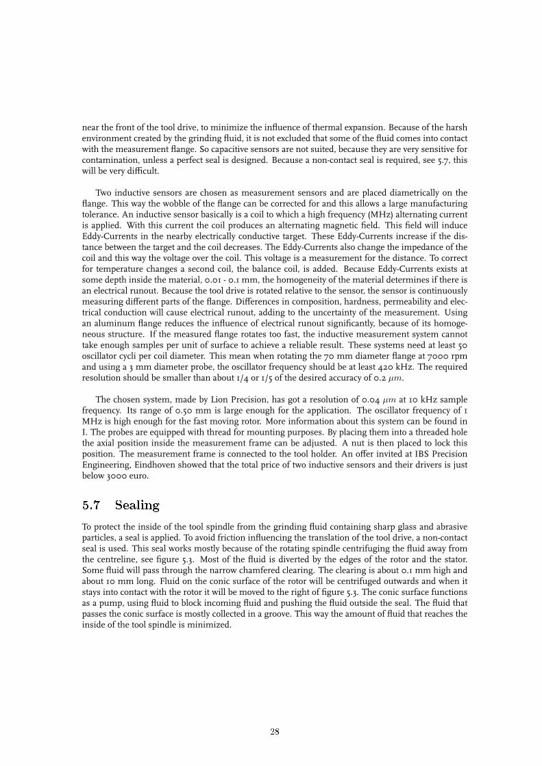
To protect the inside of the tool spindle from the grinding fluid containing sharp glass and abrasiveparticles, a seal is applied. To avoid friction influencing the translation of the tool drive, a non-contactseal is used. This seal works mostly because of the rotating spindle centrifuging the fluid away fromthe centreline, see figure 5.3. Most of the fluid is diverted by the edges of the rotor and the stator.Some fluid will pass through the narrow chamfered clearing. The clearing is about 0.1 mm high andabout 10 mm long. Fluid on the conic surface of the rotor will be centrifuged outwards and when itstays into contact with the rotor it will be moved to the right of figure 5.3. The conic surface functionsas a pump, using fluid to block incoming fluid and pushing the fluid outside the seal. The fluid thatpasses the conic surface is mostly collected in a groove. This way the amount of fluid that reaches theinside of the tool spindle is minimized.

28

Figure 5.3: Fluid �ow into tool seal

29

Chapter 6

Machine design

6.1 Introduction

In this chapter the design of the grinder is discussed using the concepts described in chapters 4 and5. First an overview of the entire grinder is given. Then the grinder is divided into subassemblies andeach of the subassemblies is discussed, first by giving an overview of the subassembly and then thecomponents are described. The first subassembly described is the tool drive, because this is one of themost important features of this machine.

6.2 Machine design overview

Figure 6.1(a) shows the base assembly, consisting of a horizontal granite slab with perpendicular toit the vertical granite slab. The base assembly is placed on isolators. Figure 6.1(b) shows the toolspindle on the horizontal granite slab. The disk on which the tool spindle stands can move along thehorizontal surface, because the bottom of the disk is suspended with an airbearing. In figure 6.1(c)the y-slide is added. This slide suspends the tool spindle disk in radial direction, and it can move iny-direction, parallel to the workpiece axis. The y-slide is suspended to the x-slide, because this allowedthe y-slide airbearings to be preloaded in a proper way. This means that the y-slide is ’floating’ abovethe granite slab. In figure 6.1(d) the x-slide is added and this completes the grinder. The x-slide issuspended by three airbearings on the horizontal slab and by two airbearings on the vertical slab. Thex-slide can move in x-direction, radial across the workpiece.

6.3 Tool drive

6.3.1 Tool drive assembly

The front (2) and back membrane (1) are centered respectively with the front (4) and back plug (9),see figure 6.2. The two plugs are centered on the tube (3) and preloaded by the M8x130 bolt. The toolconnector (7) is placed into the front plug. The tool itself (5)can then be placed onto the front plug andis preloaded with the M6x40 bolt (6). This bolt can easily be removed so the tool can be changed. Atthe back plug, the magnet for the voice coil (10) is glued onto its designated place. Each membraneis connected to the spindle rotor with 6 M2x12 bolts (8). Figure 6.2 also shows the edge (12) on theflange on the front plug that will be used for the position measurement of the tool drive.

30

(a) Base assembly (b) Adding tool spindle

(c) Adding y-slide (d) Adding x-slide

Figure 6.1: Machine design overview

1. back membrane 7. tool connector2. front membrane 8. M2x123. tube 9. back plug4. front plug 10. voice coil magnet5. tool 11. M8x1306. M6x40 12. position measurement face/�ange

Figure 6.2: Assembled tool drive

31

6.3.2 Tool drive components

Membranes

The membrane consists of two concentric 5 mm thick rings connected with a 0.25 mm thick sheet.The two rings are used for clamping this component to either the tool drive or spindle rotor. Becausethese rings are so much thicker than the sheet, when the membrane is being used and is translating,there will be no strain at the clamping zones. This prevents hysteresis, because there is no micro-slipat the clamping zone. The membranes are made from steel, because the high E-modulus, comparedto for example aluminium, allows the use of a very thin sheet having enough radial stiffness. Thisthin sheet has a low axial stiffness so a very good ratio between a high radial stiffness and a low axialstiffness can be achieved.

Figure 6.3: Membrane

Front plug

The front plug is used for centering the front membrane. The flange is used as a target for theposition sensors. The top of figure 6.4(a) shows the tool interface with a centering bore and a planeperpendicular to the centre line, so the tool can be connected properly. Also the thread is shown thatis used to connect the tool connector. The front plug is made from aluminium because of the positionsensors used. A steel plug would have caused interference as described in section 5.6. Because ofthe regular tool changes, connecting the tool bolt directly in aluminium thread would have causedproblems. The steel bolt will cut away some of the soft aluminium with each tool change, ultimatelydestroying the plug’s thread. Therefor an insert, the tool connector, is needed.

Tool connector

This 20 mm diameter steel insert has thread on the outside and is to be placed into the front plug.When placing the tool connector, some glue may be applied, to make sure it is not loosened during atool change. The inside hole has thread for the tool bolt (M6x40). A slot on top allows the connectorto be handled with a screwdriver.

32

(a) (b)1. tool centering 1. slot2. position measurement face3. membrane centering

Figure 6.4: Front plug (a), tool connector (b)

Tool

A survey of commercially available tools did not result in the findings of a suited tool. The tools foundhad large and heavy steel cones as part of their machine interface. Because the weight of the tool is amajor issue for the grinder, a custom tool is designed, see figure 6.5. The tool is centered on the frontplug with a centre edge. Tilting is prevented by the large diameter of the tool interface. The outer sideis chamfered as part of a seal, preventing the grinding fluid to reach the inside of the spindle. Theconcept is described in section 5.7. Like other cup wheels, this tool has got rounded edges.

Tube

The base of the tool drive is the tube, connecting the two membranes and the two plugs. The outerdiameter is 55 mm so it fits into the hollow air spindle rotor. Because of the limited outer diameter,a steel tube is chosen instead of an aluminium one. A thin walled steel tube weighs less than a thickwalled aluminium one, when they have the same outer dimensions and bending stiffness. The lengthof the tube will be determined as described in 6.4.1.

Back plug

The back membrane is centered on the back plug. The same centering is used to place the back pluginto the tube. Inside the plug there is room to place the voice coil magnet. There is also a threadedhole for the long bolt that preloads the two plugs onto the tube. This hole can also be used to press themagnet out of the plug in case of revision.

Voice coil magnet

The voice coil magnet goes in the fit in the back plug and is glued. If necessary the magnet can beremoved using a bolt pressing the magnet out. The datasheet of the voice coil can be found in I.

33

1. rounded edge 3. interface2. seal

Figure 6.5: Tool

6.4 Tool spindle

6.4.1 Spindle assembly

In figures 6.6 - 6.9 the different assembly steps of the tool spindle are given. Figure 6.6 shows thestator (1) and the hollow rotor (2) of the Blockhead air spindle. The datasheet of this spindle can befound in appendix I. To the front of the rotor the front membrane coupling (5) is mounted. To theback of the rotor the magnet carrier (3) with the magnets (4) and the back membrane coupling (6) areconnected. The back membrane coupling is clamped to the magnet carrier with the same bolts thatclamp the magnet carrier to the rotor.

1. air spindle stator 4. motor magnets2. air spindle rotor 5. front membrane coupling3. magnet carrier 6. back membrane coupling

Figure 6.6: Assembling the rotor

34

Figure 6.7: Adding the tool drive assembly (1)

In figure 6.7 the tool drive assembly, as described in section 6.3 is added. The alignment of the tooldrive assembly and the rotor can be adjusted, so the tool will have minimum runout. The possibilityto adjust the alignment here allows the tolerances of the parts that are centered, to be much larger. Inthis figure one can also see the bolts, that hold the membrane coupling. They can be reached whenthe membrane is in place. If the tool spindle is (partly) disassembled, the delicate membranes areprotected by the membrane couplings.

To have the membranes function properly, it is crucial that the inner and outer rings of the mem-brane are in the same plane. Any axial misalignment between the two rings will cause the axialstiffness to increase slightly. The radial stiffness is rapidly increased, so the ratio between the radialand axial stiffness deteriorates quickly. In order to get a good working membrane, the difference be-tween the axial positions of the two rings should not exceed 0.01 mm. This will give the membrane acax = 5.3 · 103N/m and a crad = 9.1 · 106N/m. There are two ways to reach this narrow axial align-ment. The first one is to specify the sizes of the rotor components with very narrow tolerances. Thiswill make the tool drive tube, the membranes, the membrane couplings and the magnet carrier verycritical components. Also the height of the air spindle should be measured, because the manufacturerspecifies a large height variation.

The other way is to partly assemble the rotor, as far as shown in figure 6.6. Then the distancebetween the outer surfaces of the two membrane couplings can be measured. So all thickness varia-tions of the assembled parts are taken into account. Knowing this distance, the tool drive tube can bemade to the right length with a tight tolerance. The exact thickness of the memranes, the membranecouplings and the magnet carrier are not important, it is important however that these parts have agood flatness.

Now the entire spindle with the tool drive assembly is placed into the toolholder front, see figure6.8. The air spindle stator has holes for bolts to mount it onto the toolholder front. The exact positionof the spindle inside the toolholder is not important, because the complete tool spindle unit will bealigned with the workpiece spindle later on.

The toolholder is closed by placing the back part onto the front part, see figure 6.9. The toolholderback holds the coil assembly for the actuation of the tool drive assembly and it also houses the motorstator. Finally the measurement frame is placed onto the toolholder front. This measurement framecontains the two position sensors that measure the position of the tool drive assembly.

6.4.2 Tool spindle components

Blockhead 4R2.25 air spindle

This air spindle built by Professional Instruments has a very low runout of 50 nm. It has got highaxial and radial stiffness, cax = 175 · 106N/m and crad = 140 · 106N/m, and can be operated at a

35

Figure 6.8: Adding spindle to toolholder front (1)

1. measurement frame 4. coil assembly2. toolholder back 5. clamp3. motor stator

Figure 6.9: Completing the tool spindle unit

maximum speed of 7000 rpm. More importantly it features a hollow rotor with an inner diameter ofabout 60 mm (2.25 inch). This allows the tool drive assembly to be placed. The Blockhead spindlehas got one radial bearing and a ring shaped axial bearing. This axial bearing prevents the rotor fromtilting. Spindles made for higher speeds usually have two radial and one axial bearing. Tilting of therotor is prevented by the two radial bearings. However the spindles constructed this way do not haveenough room for the tool drive assembly, due to their limited rotor diameter. Also high speed spindleshave less radial stiffness than the Blockhead spindle, even though they have two radial bearings. Thisis because of the smaller diameter of the rotor, the airbearing surfaces are also small. Because thisgrinder is designed primarily for research goals, achieving high speeds and thus a high productionrate is not a priority.

36

Membrane couplings

The membrane couplings are needed to enlarge the diameter of the membranes. To get a high ratiobetween the crad and the cax either the membrane should be large or it should be thin. Because itis difficult to manufacture a very thin membrane with the necessary thick outer and inner ring, themembrane should be large. The membrane coupling provides an interface for the outer membranering, the coupling itself is bolted to the mounting holes on the rotor.

Measurement frame

The measurement frame has got two functions. The main function is to provide a mounting interfacefor the inductive sensors looking at the tool drive. The two probes are placed diametrically so thewobble of the measurement flange on the tool drive can be acquired. The probes are mounted intothreaded holes and a nut on each probe is used to lock the position of the probe, when the correctdistance between the probe and the measurement flange has been set.

The second function is to shield the measurement flange of the tool drive and the air spindle fromcontamination, like grinding fluid. Therefor the edge of the measurement frame is chamfered to act asa seal as described in section 5.7. The fluid that passes the seal is collected in the first groove and sentout of the frame through a drain. The little fluid that passes the first groove is collected in the secondgroove and it also flows out through a drain. The fluid that passes the first groove can contaminatethe measurement flange. Although it is not much, it is important to choose a position measurementsystem that is insensitive for this kind of contamination.

1. chamfered seal edge 4. inductive sensor2. �rst groove with drain 5. mounting hole3. second groove with drain

Figure 6.10: Measurement frame, section view enlarged

37

Coil assembly

The coil assembly consists of three elements, see figure 6.11. The coil (4) is connected to the coilholder (3). The coil holder can be placed when the rest of the tool spindle unit is already assembled.In case of a coil failure, only the coil holder has to be disassembled. The coil holder fits into the coilholder base (2). This way the coil holder can be bolted to the holder base and the shape of the left sideof the toolholder back (1) is not important. The inside part of the toolholder back can be machined byturning from the front side. The bottom of the inside of the toolholder back will be perpendicular tothe axis of rotation with a very tight tolerance. The axis of rotation of the relatively short holder base isaligned by its wide flange. Finally the coil holder is placed inside the holder base. The coil holder alsofunctions as an end stop for the tool drive. This way high stresses on the membranes are prevented, ifa large axial force is pushing on the tool. The axial position of the coil holder can be adjusted by usinga spacer, placed between the coil holder and the holder base.

1. toolholder back 4. voice coil, coil2. coil holder base 5. voice coil, magnet3. coil holder

Figure 6.11: Coil assembly

6.4.3 Motor stator

The stator of the motor that rotates the tool consists of coils and iron. The exact shape of the statorneeds to be determined but its size is comparable to other motor stators with the same power andspeed. It is also necessary to build in three Hall-sensors with the stator. These sensors are neededto control the rotational speed of the rotor. Because only the speed has to be controlled, not the exactposition, it is not necessary to use an expensive, high resolution encoder. The Hall-sensors should besufficient.

6.4.4 Toolholder front

The outer shape of the toolholder front, shown in figure 6.12, is milled first. The mounting holes (4),(6) are also made. Then the toolholder front is placed in a lathe, so the fit for the air spindle (3) andthe hole for the rotor (2) can be made. Also an edge is made to centre the toolholder back (7). This

38

way the toolholder front and back can be aligned, so the motor stator and the voice coil fit properlyaround the spindle rotor. At the front side the centre edge for the measurement frame (1) is machined.

1. edge measurement frame 5. free space2. rotor hole 6. mounting hole toolholder back3. edge air spindle 7. edge toolholder back4. mounting hole air spindle

Figure 6.12: Toolholder front

1. edge motor stator 4. �attened part2. edge coil assembly 5. clamp hole3. hole coil assembly

Figure 6.13: Toolholder back

39

6.4.5 Toolholder back

The toolholder back is made from bar stock. On a lathe the edge on which the motor stator is placed(1), is made. Then the edge (2) and the hole for the coil assembly (3) is made. On a milling machinethe flattened part (4)is made. The flattened part features an elevated part, so only the back end of thetoolholder comes into contact with the tool disk on which it is placed. Finally a clamping area (5) ismilled, so the tool spindle can be mounted on the tool disk.

6.5 Tool disk

6.5.1 Tool disk assembly

Onto the disk base (4) the grafite parts of the radial (5) and axial bearing (6) are placed, see figure6.14. Also the disk drive coils (2) are mounted to the side of the disk base. Inside the vacuum seal(7) is placed and it is pressed onto its place by the disk top (3). Beneath the vacuum seal is a roomwith underpressure, the vacuum chamber (8). This preloads the axial airbearing. The bottom of thevacuum chamber is sealed with a narrow gap surrounded with an atmospheric groove (9). Finally thetool spindle can be placed onto the three mounting holes (1). Two holes are at the front side of the toolspindle and one is at the rear.

6.5.2 Tool disk components

Vacuum chamber

To preload the tool disk, an airbearing placed at the opposite side of the horizontal granite slab canbe used. However if the bearings are directly opposite to each other, a very large structure is needed,adding a large amount of - moving - mass. Reducing this mass by placing the preload bearing more tothe edge of the granite slab, will induce bending of the slab, which is very disadvantageous. Thereforthe choice is made to preload the tool disk using vacuum, [Ver99]. In this thesis ’vacuum’ meansa relative underpressure of maximal 0.6 bar ( 0.4 bar absolute). To limit the amount of air flowingthrough the vacuum chamber and thus limiting the required power for the pump, the vacuum cham-ber needs to be sealed. At the bottom of the disk, this requires a narrow gap that is long enough so alaminar flow goes through. A turbulent flow will induce unwanted disturbing forces on the disk. Theperimeter of the vacuum chamber, w, is 0.93 m, the length of the seal (in radial direction), l, is 8.5mm. The flow rate Q can be calculated using

Q =∆p

R=

wh3

12µlpu (6.1)

with µ is the dynamic viscosity of air, which is 17 · 10−6Pa · s, pu the relative underpressure of0.6bar and h the gap height of 5µm. This gives a value of Q = 1.64 · 10−5m3/s. Using the densityof the air at the underpressure being ρu = ρatm(1 − pu/patm) the Reynolds number, Re, can becalculated with

Re =Q

w

ρu

µ(6.2)

Using the parameters mentioned it can be shown that Re = 0.54 and because this is lower thanthe laminar-turbulent transition value of 2000, the flow is laminar. The vacuum seal at the bottom ofthe tool disk will work properly.

Because the disk base basically is a thick walled tube, the top of the centre hole needs to be sealedas well to create a vacuum chamber. This is done with a vacuum seal consisting of a thin sheetand a mounting ring. The ring is axially pressed onto an edge inside the disk base. Because of theunderpressure beneath the vacuum seal the atmospheric pressure will try to push the seal downward.If instead of the seal a simple disk was used to seal the vacuum chamber, see figure 6.15(a), bending

40

1. mounting hole 6. gra�te axial bearing2. coil disk drive 7. vacuum seal3. disk top 8. vacuum chamber4. disk base 9. atmospheric groove5. gra�te radial bearing

Figure 6.14: Tool disk assembly

of the disk by the atmospheric pressure would have caused the tool disk to deform radially. Also alot of material is needed to reduce the bending stress to an acceptable level. Such an aluminium diskwould weigh about 2 kg. Figure 6.15(b) shows a schematic view of the vacuum seal as used in thedesign. The thin sheet can resist forces only in its plane. Because the sheet is fixed in axial directionto the mounting ring, the force applied by the sheet onto the mounting ring, thus also on the tooldisk, is in axial direction. The force generated by the atmospheric pressure will cause minimal radialdeflection. This radial deflection would have caused the axial tool disk bearing to tilt relative to thegranite base. Because the sheet is shaped almost like a sphere, stresses are low and a sheet of 2 mmthick aluminium is sufficient, see E.6. This is because there is only tension and no bending, so thematerial is optimally used. The weight of the vacuum seal is reduced to 0.5 kg.

6.6 Y-slide

6.6.1 Y-slide assembly

The base of the y-slide is an aluminium block to which airbearings are connected using cardan joints,see figure 6.16. A cardan joint reduces the tilt stiffness of the airbearing connection, allowing theairbearing to align parallel with the guideway. This way themounting of the airbearing is less critical inorder to avoid it getting jammed with the guideway. The gap between the airbearing and the guideway

41

(a) (b)

Figure 6.15: (a) Preloading causes radial displacement, (b) Radial displacement minimized

is about 5 µm. The large airbearings (1) are preloaded with other large airbearings (2) that have a farless stiff connection. This way the preload bearings provide a constant force, instead of stiffness andthis way an overconstrained situation is prevented. These large airbearings play an important role inthe grinding process, because they play a part in the angle in Rz-direction and in the x-position. Thesmall airbearings (3) however do not play a significant role in the grinding process, they just have toconstrain the other DOF’s of the y-slide. Their main task is to avoid low frequency vibrations of they-slide and to prevent the y-slide from tilting so much that the airbearing ring, (5), runs into contactwith the tool spindle disk. The small airbearings, (3), have a stiffness of c = 5.2 · 107N/m each andwith the total mass of the y-slide being 58 kg, the lowest eigenfrequency of the y-slide on its bearingsis 261 Hz. The tool spindle disk will be radially suspended in the airbearing ring. This ring is madefrom steel to minimize its size and hereby minimizing the distance between the centre line of the diskand the workpiece. Also because this is a rotationally symmetric piece, it can be machined or groundinto shape with the accuracy needed for a proper air gap. The bottom of the ring is bolted to the y-slidebase. The strip of magnets for the tool spindle disk drive (6) is placed at the bottom of the base, thisway the airbearing ring can be as close to the centre of mass of the tool spindle unit as possible, inz-direction. Finally the coils of the linear motor actuating the y-slide (7) are placed on the centre lineof the base. This way no momentum is applied to the slide when it is being actuated, resulting in lesstracking error. The coils are attached to the top of the base to minimize the distance between the lineof the coil and the centre of mass of the y-slide and tool spindle unit.

6.6.2 Y-slide components

Measurement system

The position of the x- and y-slides are measured by a system connected to the y-slide, as described insection 4.4. A sensor on the horizontal granite slab determines the position of a grid at the bottomside of the y-slide. This way any x-frame errors in y-direction and any y-frame errors in x-direction aremeasured directly. This would not have been the case if each slide had its own separate scale.

The planar measurement system is the Nanogrid made by Optra, for a complete datasheet see I.The working principle is show in figure 6.17. A laser beam is directed via a prism to the xy-grid. Atthe grid diffraction takes place and the ± 1st orde diffracted beam in both x and y direction is collectedby the lens. The horizontal and vertical beams are then collected with a sensor and the fringe patternis processed.

Because of the relatively large x- and y-stroke the standard solution made by Optra would havegiven an accuracy of ± 1 µm. This way the desired accuracy can not be achieved. Communicationswith the people at Optra showed that there is a possibility to use their high accuracy, small sized gridwith multiple sensor heads. When the grid is moved almost out of range of one sensor, it comes intorange of another sensor. On certain x- and y-positions there are two or more sensorheads lookingsimultaneously at the grid. Such a system has an accuracy of ± 35 nm, sufficient for the grinder. The

42

1. large airbearing 5. airbearing ring2. preload large airbearing 6. disk drive3. small airbearing 7. y-slide drive4. preload small airbearing

Figure 6.16: Assembled y-slide

sensorheads are mounted onto the horizontal granite slab, which makes the position of the sensor-heads thermally stable, because of the large mass of the slab. Changes in the surrounding temperaturewill cause changes in the length of the slab on such a long time scale, it will be possible to calibratethe distance between the sensorhead and the workpiece between grinding steps.

Figure 6.17: Nanogrid measurement principle

Y-slide drive

The y-slide is being actuated with an ironless linear motor. Because there is no physical contact be-tween the two moving parts of the motor, there is no friction. Friction, together with the finite stiffnessof the slide, causes virtual play, reducing the resolution of the drive. There are several reasons to preferan ironless linear motor above a ball screw drive. First off all, a ball screw drive suffers from play and to

43

correct this a preloaded nut can be applied. But this creates additional friction and so increases virtualplay. Also the ball screw nut should be mounted in a proper way, like [Suz95] did. For his precisiongrinder, he designed a coupling consisting of flexures, unconstraining all DOF’s except the translationof the drive axis. This way the position of the y-slide is not overconstrained. Such a coupling must bemanufactured carefully. Another type of coupling is described by [TUe02]. A tube is cut-out at fourlateral positions so a cardan joint is created. This cardan joint has a high axial stiffness and a hightorsion stiffness. This fairly easily made component adds some length to the ball screw drive, but thedrive is no longer overconstrained. Some advantages of a ball screw are that it is an indirect drive, sothe motor used can produce a small torque at high speeds. This results in the use of a small motor thatneeds less current and thus produces less heat. A ball screw is also stiff above the bandwidth of thecontroller, a linear motor is not. An ironless motor, finally, does not have magnetic attraction betweenthe two motor parts, as ironcore linear motors do. Ironless motors however have a lower force pervolume unit than ironcore motors have. Moving the 100 kg weighing y-slide with tool spindle unit 5mm at 1 Hz will require a force of 20 N. Adding the grinding force of maximum 1 N and a neglectableamount of friction force caused by the airbearings, an actuator of more than 21 N is sufficient.

Disk drive

The drive that actuates the tool disk resembles the y-slide drive. The coil is placed onto the tool diskand its windings are in the same way as in a disk armature motor. Instead of a translation like with they-slide drive, a -partly- rotation is actuated. The magnets are placed on the y-slide and are orientatedaround the tool disk.

6.7 X-slide

6.7.1 X-slide assembly

The somewhat U-shaped x-slide, see figure 6.18, holds the y-slide near its centre line (4) so the tiltingstiffness provided by the two y-airbearings (1) is maximized. The x-slide stands on three airbearings(2), suspending it on the horizontal plane. The y-slide guideways (3) are connected to either the leftor right side of the frame. Some room was made so the preload airbearings of the y-slide can passthrough. The magnets for the y-slide drive (4) are mounted on the centre line of the frame. The x-slidecoils (5) are placed at the bottom of the right part of the frame. On top of the frame there is a top plate,for clarity reasons this plate is not shown in figure 6.18.

6.7.2 X-slide components

X-slide frame

Figure 6.19 shows the wire model of the x-frame with its system points. These points are used tomount parts to the frame and should be connected to each other in a stiff way. At the edge of theframe, the airbearings are mounted (1). This gives a high tilting stiffness, the large distance betweenthe airbearings at the bottom side of the figure is especially important for the grinding process. Eachof the y-slide guideways are connected at two points (2) so a line can be described for each guideway.The line, described by the two points of the x-slide drive coil (3), points at the centre of mass of all themoving slides. This way, when actuating the x-slide, no momentum is created that rotates the slide.Also the line described by the two points for the y-slide drive, points at the centre of mass of the y-slideand tool spindle unit. The system points are connected with lines in such a way that triangles arecreated. Finally aluminium is placed around the lines creating a physical frame. The lowest eigen-frequency is 257 Hz, at this mode the end points of the two ’legs’ of the U-shape are symmetricallymoving sideways, see E.2. The stiffness of the frame in y-direction is cy = 3.3 · 108N/m.

The frame assembly consists of three pieces, one centre piece and two side pieces. The connectinginterfaces are just above the y-slide guideways. They are all milled from blocks of aluminium, this

44

1. y-airbearings 4. y-slide drive2. z-airbearings 5. x-slide drive coils3. y-slide guideway

Figure 6.18: Assembled x-slide

way good interfaces can be made. The three frame pieces, the y-slide guideways and the five x-slideairbearings can be placed almost with machine accuracy. A frame made from many plates has tobe assembled carefully and the interface areas for the airbearings and the y-slide guideways have toundergo final processing. Because there will be built only one of this grinder, the removal of theamount of material is not an important issue. Between the two interface areas of the three framepieces, and between these three pieces and the top plate, silicone paste is applied. This paste is ableto dampen frame vibrations, the aluminium is not able to do so. Inside the grinder there are manysources creating frame vibrations. First of all, the grinding process causes vibrations, because of thetool-workpiece interaction. The runout of the tool and the interaction of the different grains with theworkpiece causes excitations. Secondly, the actuator forces moving the slides also cause vibrations. Ifall this kinetic energy is able to accumulate inside the machine frame, the amplitudes of the vibrationswill increase. This can result in an unstable grinder and this will decrease the shape accuracy ofthe ground products. By using a material that is able to dissipate this energy, this instability can beprevented. The paste is not applied onto system points, so it does not decrease the frame stiffness.This is illustrated in figure 6.20, it shows part of the x-frame. The system points are connected toeach other through clamp zones. Because of the high contact pressure, there is little or no hysteresisat these zones. Between the system points there are damping zones. Small amounts of material areremoved from the x-frame, so spaces are created between the frame parts. These spaces are filledwith paste. Because silicone paste, like other damping materials, behave in a viscoelastic way, the

45

dissipated energy depends only on the velocity of the frame part. When this velocity is reduced tozero, the material is returned to it’s nominal position, so there is no virtual play.

1. airbearing 3. x-slide drive coil2. y-guideway 4. y-slide drive

Figure 6.19: Wire model of x-frame with system points

Airbearings

Airbearings, or aerostatic bearings, are know for their frictionless movement and are used in manyprecision applications. In order to get a stiff bearing, the airbearing must be preloaded against a sur-face. There are several ways to do this. One can use the weight of the machine part that is carried bythe bearing, but this does not allow fine tuning the bearing by adjusting the preload force. Anotherway is to use a preload airbearing at the other side of the guideway, this is done with the y-slide asshown in 6.6. For the x-slide however the preload brackets would have been very large, because theywill have to reach the other side of the 300 mm thick granite block. Also the bottom of the horizontalslab must be smooth and flat enough to allow the preload bearing to work. For this reasons the choiceis made to preload the bearing using vacuum (underpressure).

A number of different airbearings were examined in [Ver99]. Two of these looked very interestingfor the grinder because of their stiffness, their manufacturing process and the way a vacuum cham-ber can be integrated. These two bearings are shown in figure 6.21. The one on the left is a bearingconsisting of porous grafite. The grafite works as many restrictors. The one on the right is a bearingwith a parallel gap between the bearing and the surface, and it has a grafite insert as a restrictor. Thisdisk spreads the pressure of the flowing air more than a bearing with a single hole restrictor. Theproperties of bearing with a single hole restrictor may deteriorate when the restrictor is above a crackin the under laying surface. Because that surface is made from granite, it expected that some of thesecracks exists. Bearings with porous restrictors are insensitive to these cracks.

46

1. Clamping zone 2. Damping zone

Figure 6.20: Frame interface

The properties of the two bearings are stated in table 6.1. It shows that the optimal stiffness thatcan be acquired per unit of surface is slightly higher with the porous grafite bearing. But this alsorequires a larger preload force. Because of this higher preload force, the actual bearing surface of theporous grafite bearing may be smaller, the required vacuum surface is many times larger than thesurface of the grafite insert bearing. The total amount of bearing surface of the grafite insert bearingis about three times smaller than that of the porous grafite bearing. So the choice is made to use theparallel gap bearing with a grafite insert.

Figure 6.21: Left: porous gra�te bearing, right: parallel gap bearing with gra�te insert

Bearing type Porous gra�te bearing Gra�te insert 8mmcopt/A 1.8 1.6 [N/µm/cm2]

F (copt)/psA 0.66 0.15 [−]F (copt) 3.6 0.8 [kN ]Abearing 83 94 [cm2]Avacuum 590 135 [cm2]Atotal 673 229 [cm2]

Table 6.1: ps = 6.0 bar, cbearing = 150N/µm, the pressure in the vacuum chamber is 0.4 bar.

47

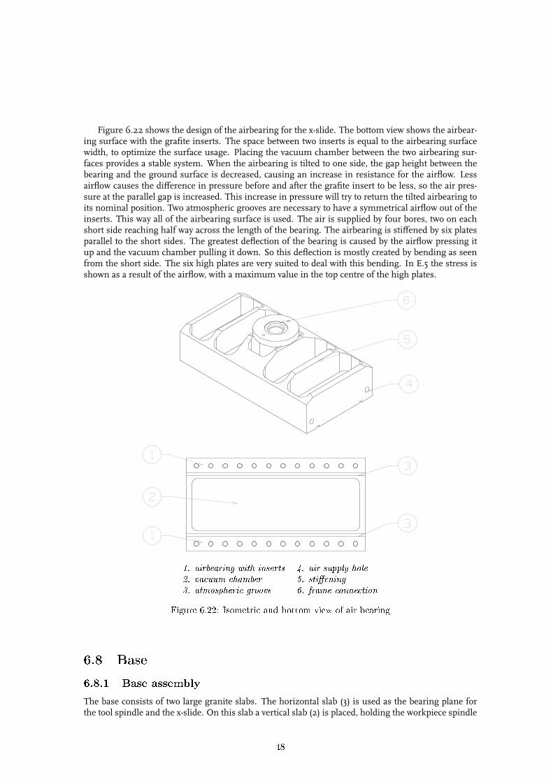
Figure 6.22 shows the design of the airbearing for the x-slide. The bottom view shows the airbear-ing surface with the grafite inserts. The space between two inserts is equal to the airbearing surfacewidth, to optimize the surface usage. Placing the vacuum chamber between the two airbearing sur-faces provides a stable system. When the airbearing is tilted to one side, the gap height between thebearing and the ground surface is decreased, causing an increase in resistance for the airflow. Lessairflow causes the difference in pressure before and after the grafite insert to be less, so the air pres-sure at the parallel gap is increased. This increase in pressure will try to return the tilted airbearing toits nominal position. Two atmospheric grooves are necessary to have a symmetrical airflow out of theinserts. This way all of the airbearing surface is used. The air is supplied by four bores, two on eachshort side reaching half way across the length of the bearing. The airbearing is stiffened by six platesparallel to the short sides. The greatest deflection of the bearing is caused by the airflow pressing itup and the vacuum chamber pulling it down. So this deflection is mostly created by bending as seenfrom the short side. The six high plates are very suited to deal with this bending. In E.5 the stress isshown as a result of the airflow, with a maximum value in the top centre of the high plates.

1. airbearing with inserts 4. air supply hole2. vacuum chamber 5. sti�ening3. atmospheric groove 6. frame connection

Figure 6.22: Isometric and bottom view of air bearing

6.8 Base

6.8.1 Base assembly

The base consists of two large granite slabs. The horizontal slab (3) is used as the bearing plane forthe tool spindle and the x-slide. On this slab a vertical slab (2) is placed, holding the workpiece spindle

48

1. workpiece spindle 5. sensor y-slide2. vertical granite slab 6. magnet x-slide drive3. horizontal granite slab 7. vacuum bore4. isolator (1 of 4)

Figure 6.23: Base assembly

(1). The horizontal slab contains space for the position sensors of the y-slide and the magnets ofthe x-slide drive. Also four brackets are bolted to the horizontal slab for the isolator connections (4).Finally holes (7) are drilled into the granite, providing underpressure to the bearings suspending thetool disk and the x-slide. If vacuum was applied through cables, very thick cables would be needed toprevent the atmospheric pressure from squeezing the cables. These thick, stiff cables cause disturbingforces when the slides are being moved. Applying vacuum through a bore prevents the need of havingmoving cables at the top side of the grinder. The cables placed at the end of the vacuum bores, leadingto the pump, can be properly concealed beneath the machine.

6.8.2 Base components

Granite blocks

The properties of the granite are given in I. Granite is often used for precision instruments likeCMM’s, because very flat surfaces can be created, less than 1 µm/m2. Also the large solid blocks arethermally very slow, so changes in temperature do not result in length changes quickly.

Isolator system

Vibrations caused by the environment of the grinder, e.g a passing truck or a slamming door, cancause shape errors on the workpiece. Therefor the grinder has to be isolated by placing it on springswith very low stiffness. Such a situation is given in figure I where a mass is placed onto two springs.The centre of mass Mc is distance h above the line between the isolators. When the machine is tiltedwith angle β the sum of the momentum on point A is

ΣMa = FcL + FcL−mgh sin(β) (6.3)

49

m[kg] or J [Nm/s2] feig

x-translation 3200 1.5y-translation 3200 1.5z-translation 3200 1.0

Table 6.2: Lowest eigenfrequencies of isolated grinder

ΣMa = 2cL2 sin(β)−mgh sin(β) > 0 (6.4)

2cL2 > mgh (6.5)When equation 6.5 is true the forces applied by the two springs will be able to push the mass back

to the nominal position and there is a stable system. The distance h on the grinder is reduced toalmost zero by placing the isolator brackets as high as possible on the horizontal slab. The centre ofmass of the entire machine is just below the top surface of the horizontal slab, so the isolator systemis stable. The isolator brackets are placed in such a way that the roll frequency in the x- and y-directionis about the same. Table 6.2 shows the lowest eigenfrequencies in x-, y- and z-direction. Figure 6.25shows the weight on each of the isolators,

Mc

C C

L L

A

h

β

mg

Fc

Fc

Figure 6.24: Analyzing an isolated body

Figure 6.25: Weight per isolator (kg)

50

1. vertical granite slab 4. mounting ring2. air spindle stator 5. horizontal granite slab3. air spindle rotor

Figure 6.26: Workpiece spindle in base

Workpiece spindle

The workpiece spindle is a motorized Blockhead 10R. This spindle features a high stiffness, cax =1750 · 106N/m and crad = 350 · 106N/m and a runout of less than 25 nm. The spindle shouldhave an accurate position encoder, so free-form features may be ground at the right position on theworkpiece. Themounting ring allows the top surface of the stator to be aligned with the vertical graniteslab surface. This minimizes thermal length and creates a stable workpiece position. The use of themounting ring also simplifies the manufacturing process. The vertical granite slab can have a roughthrough hole. The mounting ring can be made with a very good flatness, so it connects well with boththe granite and the spindle. It is difficult to mill precision counterbores in granite. By moving themounting ring, the workpiece spindle can be aligned and fixed. The mounting ring is bolted to thevertical slab using inserts.

51

Chapter 7

Conclusions and recommendations

7.1 Conclusions

When grinding brittle glass in a ductile way, the quality of the surface is improved, because of theabsence of subsurface damage. This reduces polishing time and this is especially important for free-form optics. These optics can be polished only locally and it is a great amount of work just to improvethe surface roughness, let alone remove subsurface damage. A grinder that features a controllablegrinding force, so subsurface damage is prevented, is necessary for TNO to improve the manufactur-ing process of single piece optical components. The grinder should also be able to grind free-formoptics with a good shape accuracy so they can be used for scientific and industrial purposes.

A precision grinder with a controlled-force tool spindle is designed. The tool spindle is designedin such a way it can be used for experiments on an existing platform. This tool spindle features arotor with an elastic guideway inside. This guideway is actuated with a voice coil which can apply a setforce. To reduce the influence of inertial forces of this guideway on the grinding process, the amountof mass is minimized. For the workpiece to get a good shape accuracy the position of the tool driveis measured using two inductive sensors. These sensors provide the information for the voice coil toeither keep applying force on the workpiece or to stop because the desired shape is achieved.

The tool spindle is mounted on a large diameter disk that is suspended with an airbearing on agranite surface. This way the only DOF’s that need to be unconstrained are not constrained. To actu-ated these constrains the tool disk is hold by the y-slide. This relative fast slide allows the grinder tomake free-form features into rotational-symmetric workpieces. The y-slide is hold by the slow x-slide,that continuously moves radially across the workpiece surface.

By measuring the position of the y-slide directly from the granite base, many errors of the x- andy-slides can be measured. This improves the accuracy of the grinder and the desired accuracy isachieved.

Finally calculations are made showing that the required accuracy is achieved and the grinder has agood dynamical behavior.

7.2 Recommendations

Motor stator

The design of the tool spindle is emphasized so shortly after the completion of this thesis, experimentscan begin examining the potential of controlled-force grinding. The motor stator however still needsto be determined. The outer dimensions have been estimated, so enough room is reserved. This

52

estimation was done by looking at the dimensions of similar motors and motors with more power. Sothis will not have a big impact on the spindle design.

Support frame

To load and unload the grinder properly, an operator support frame is needed, see figure 7.1. It mustsupport the operator in a partly lying position. It also must prevent people from leaning onto themachine, tilting it on its isolators. This can easily bring one of the isolators to the end of its stroke.Then surrounding vibrations will not be resisted and will cause workpiece errors. The support framecan be made from tubes and plates welded together to limit the weight. The interface with the operatorshould be adjustable in height and angle, so the working position can be customized for each operator.Also a cover is needed to shield the surroundings from the grinding fluid. Especially the airbearingsneed good covering to prevent them from being scratched. A scratch can reduce the performance ofthe bearing.

Figure 7.1: Support frame recommendation

Optimization and detailing

Some optimization can still be done to the design of the grinder. This includes improvement of themanufacturability, so parts can be made in an easier way, saving time and money. Also some machineparts need more detailing, such as the way the isolators are connected to their brackets. The positionof the mounting holes and the bolts that should be used are not determined yet.

53

Bibliography

[Bif91] T. G. Bifano, Ductile-regime grinding: a new technology for machining brittle materialsJournal of Engineering for Industry, Vol 113, pag 184-189, (1991)

[Bla88] P. Blake, Precision machining of ceramic materialsCeramic Bulletin, Vol 67, pag 1038-1044, (1988)

[Bol99] B. P. A. Bollen, Een ontwerp van een machine voor het fabriceren van asferische lenzen, volgensde methode van W.A.G.N.E.R.Master thesis, Technisch Universiteit Eindhoven, reportnumber PE99-022, (1999)

[Boo03] Silvia M. Booij, Fluid jet polishingPhD thesis Delft University of Technology, (2003)

[Cou04] Jermiah A. Couey, Eric R. Marsh et al., Monitoring force in precision cylindrical grindingPrecision Engineering, Vol. 29, pag 307-314, (2004)

[Fäh98] Oliver W. Fähnle, Shaping and finishing of asperical optical surfacesPhD thesis Delft University of Technology, (1998)

[Fäh99] O. W. Fähnle, H. van Brug, Novel approaches to generate aspherical optical surfacesProceedings of SPIE, Vol 3782, pag 170-180, (1999)

[Fan04] F. Z. Fang, G. X. Zhange, An experimental study of optical glass machiningInt J Adv Manuf Technol, no 23, pag 155-160, (2004)

[Fis00] Anthony C. Fischer-Cripps, Introduction to contact mechanicsSpringer-Verlag New York Inc., (2000)

[Fra91] Jelm Franse, Aspects of precision grindingPhD thesis, Technisch Universiteit Eindhoven, (1991)

[Hal04] Layton C. Hale, Testing a low-influence spindle drive motorPrecision Engineering, Vol 29 pag 1-10, (2004)

[Hah64] R. S. Hahn, Controlled-force grinding, a new techique for precision internal grindingJournal of Engineering for Industry, Vol 86, pag 287-293, (1964)

[Heg00] J. B. J. W. Hegeman, Fundamentals of grinding, surface conditions of ground materialsPhD thesis Rijksuniversiteit Groningen, (2000)

[Hen05] Rens Henselmans, Nick Rosielle et. al., Design of a machine for the universal non-contact mea-surement of large free-form optics with 30 nm uncertaintyProceedings of SPIE, Vol 5869 pag 586919-1 - 586919-12, (2005)

[Höl02] W. Höland, G. Beall, Glass-ceramic technologyThe American Ceramic Society, Westervill, Ohio, (2002)

54

[Kar93] H. H. Karow, Fabrication methods for precision opticsJohn Wiley and Sons Inc, New York, (1993)

[Kra] H. J. J. Kraakman, Precisie produktie, "Hoe en waarmee"?Philips Centre for Manufacturing Technology, CFT Mechatronics

[Lam97] J. Lambropoulos, Subsurface damage in microgrinding optical glassesUniversity of Rochester, LLE Review, Vol 73, pag 45-49, (1997)

[Law77] B. R. Lawn, A model for crack initiation in elastic/plastic indentation fieldsJournal of Materials Science, Vol 12, pag 2195-2199, (1977)

[Law80] B. R. Lawn, A. G. Evans, Elastic/plastic indentation damage in ceramics: The median/radialcrack systemJournal of the American Ceramic Society, Vol 63, no 9-10 pag 574-581, (1980)

[Law95] Brian Lawn, Fracture of brittle solids - second editionPress Syndicate of the University of Cambridge, (1995)

[Li98] K. Li, Y. Shapiro, J. C. M. Li, Scratch test of soda-lime glassActa mater., Vol 46, No 15, pag 5569-5578, (1998)

[Mal89] S. Malkin, Grinding technology, theory and application of machining with abrasivesEllis Horwood Limited, Chichester, West Sussex, England, (1989)

[Mee05] M. Meeder, W. A. C. M. Messelink, O. W. Fähnle, Analysis of the ductile-brittle transition inloose abrasive grindingProceedings of SPIE, Vol 5869, pag 58690M-1 - 58690M-6, (2005)

[Mül98] H. K. Müller, B. S. Nau, Fluid sealing technology, principles and applicationsMarcel Dekker Inc, New York, (1998)

[Nam89] Y. Namba, Ultra-precision surface grinder having a glass-ceramic spindle of zero-thermal expan-sionAnnals of the CIRP, Vol 38(1) pag 331-334, (1989)

[Pau87] P. Paul, D. F. Edwards, Optical glass fabrication technology. 2: Relationship between surfaceroughness and subsurface damageApplied optics, Vol 26, no 21 pag 4677-4680, (1987)

[Qia04] J. Qian, P. Vleugels, A novel design for a high precision freeform ELID grinding-machineProc. of 4th euspen international Conference-Glasgow, Scotland(UK), (May-June 2004)

[Row83] W. B. Rowe,Hydrostatic and hybrid bearing designButterworth&Co, London, (1983)

[Sch98] P. Schellekens, N. Rosielle, et. al., Design for precision: Current status and trendsAnnals of the CIRP, Vol 47(2) pag 557-586, (1998)

[Sha96] Milton C. Shaw, Principles of abrasive processingOxford University Press Inc., New York, (1996)

[Suz95] H. Suzuki, S. Murakami, An ultraprecision grinding machine for non-axisymmetric asphericmirrorsNanotechnology, Vol 6 pag 152-157, (1995)

[TUe02] Lecture note 4007 (in Dutch), Constructieprincipes 1Eindhoven University of Technology, (2002)

55

[TUe03] Lecture note 4U700 (in Dutch), Uitreikbladen nauwkeurigheid van machinesEindhoven University of Technology, (2003)

[Ver99] Hans Vermeulen, Ceramic optical diamond turning machinePhD thesis, Technische Universiteit Eindhoven, (1999)

[You87] M. Younis, M. M. Sadek, T. El-Wardani, A new approach to development of a grinding forcemodelTransactions of the ASME, Journal of Engineering for Industry, Vol. 109, pag 306-313, (1987)

56

Notation

Symbol Unit DescriptionAc [m2] Tool contact aread [m] Penetration depth, depth of cut, infeeddc [m] Critical penetration depth

dmax [m] Maximum infeed for grinderE [Pa] Young's modulusEc [J ] Energy needed for crack formationEp [J ] Energy needed for plastic deformation of workpieceFc [N ] Cutting grinding forceFc [N ] Force applied by spring with sti�ness cFn [N ] Normal grinding forceFnc [N ] Part of normal grinding force needed for cuttingFnp [N ] Part of normal grinding force needed for ploughingFnr [N ] Part of normal grinding force needed for rubbingH [Pa] HardnessKc [Pa

√m] Fracture toughness

k1 [N/mm2] Chip thickness coe�cientKl [ N

unitLa

2] Loading force coe�cient

La [−] Loaded tool area / total tool areaLc [m] Tool contact lengthp [Pa] PressureR [m] Radiusvt [m/s] Tool speedvw [m/s] Workpiece speedw [m] Width of cut

α [◦] Angle between tool and workpieceαf [ N

mm2 ] Ploughing grain coe�cientν [−] Poisson ratio

Table 7.1: Notation

57

Appendix A

Assembly drawings

Figure A.1: Assembly views

58

1. workpiece 4. base2. tool spindle 5. isolator3. x-slide

Figure A.2: Assembly trimetric view

59

Figure A.3: Assembly views of tool spindle

60

1. air spindle stator 7. toolholder front2. air spindle rotor 8. motor stator3. measurement frame 9. motor rotor4. front membrane (inner ring) 10. back membrane (inner ring)5. tool 11. voice coil6. measurement �ange/face 12. toolholder back

Figure A.4: Section view of tool spindle

61

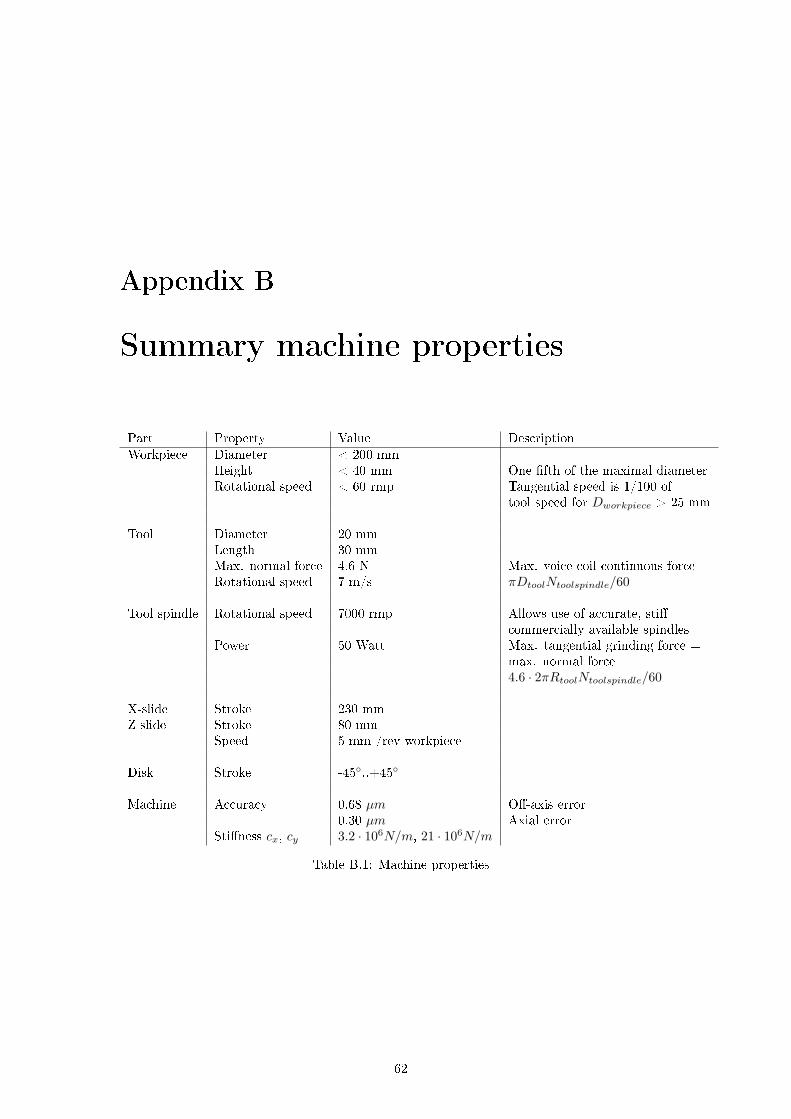
Appendix B

Summary machine properties

Part Property Value DescriptionWorkpiece Diameter < 200 mm

Height < 40 mm One �fth of the maximal diameterRotational speed < 60 rmp Tangential speed is 1/100 of

tool speed for Dworkpiece > 25 mm

Tool Diameter 20 mmLength 30 mmMax. normal force 4.6 N Max. voice coil continuous forceRotational speed 7 m/s πDtoolNtoolspindle/60

Tool spindle Rotational speed 7000 rmp Allows use of accurate, sti�commercially available spindles

Power 50 Watt Max. tangential grinding force =max. normal force4.6 · 2πRtoolNtoolspindle/60

X-slide Stroke 230 mmZ-slide Stroke 80 mm

Speed 5 mm /rev workpiece

Disk Stroke -45◦..+45◦

Machine Accuracy 0.68 µm O�-axis error0.30 µm Axial error

Sti�ness cx, cy 3.2 · 106N/m, 21 · 106N/m

Table B.1: Machine properties

62

Appendix C

Tool spindle cost

Here the estimated cost of the tool spindle are given. Table C.1 gives an overview of the cost.

Air spindle

The air spindle used is a Blockhead 4R2.25, made by Professional Instruments. The price of 5000 eurois based on the price of the Blockhead 4R, which is a similar spindle, only with a smaller diameter holein the rotor. The price of the 4R is 5000 dollar and taken into account a slightly higher price for thelarger rotor hole, additional cost like shipping, the price of 5000 euro is estimated.

Motorization air spindle

The costs of motorizing the air spindle is estimated at 12000 euro. This is based on the prices of themotorization of other Blockhead air spindles. Because of the relatively low power needed from themotor, the real price is expected to be lower than the estimated price.

Inductive measurement system

The chosen inductive measurement system is the ECL100-U3B-10kHz-SAM made by Lion Precision.An offer invited at their representative at IBS Precision Engineering in Eindhoven, showed that theprice of one system is 1500 euro. The total price for two systems is 3000 euro.

Fabricated parts

It is more challenging to estimate the cost of the parts that are to be custom fabricated, than the partsthat can be bought. The cost of the fabricated parts depends heavily on the desired manufacturingtolerances. Tight tolerances require more time for loading the part into a machine, additional stepssuch as heat treatment may be necessary and the amount of material removed per time unit is smaller.Because the exact tolerances of the spindle part are not known at this time, it is possible to make onlya rough estimation of the cost. These parts will cost 5000 - 10000 euro. Additional cost to assemblethe tool spindle also have to be made.

Part Cost (euro)Air spindle 5.000Motorization air spindle 12.000Inductive measurement system 3.000Fabricated parts 10.000Total cost 30.000

Table C.1: Overview cost tool spindle

63

Appendix D

Dynamical model

In order to study the dynamical behavior of the entire grinder, a dynamical model has been made.This model is shown in figure D.1. All the bodies of the model can move in x-direction (horizontally),in y-direction (vertically) and can rotate along the z-axis, φ. The relatively stiff frame parts are modeledas rigid bodies, where as the airbearings between the different slides are modeled as springs. This waya relatively simple model is produced, giving a fairly good estimation of the lowest and thus the mostimportant eigenfrequencies.

The tool drive is represented with the first mass, with m1, J1. It is suspended in x-direction witha spring with stiffness cx1 and suspended in y-direction with a spring with stiffness cy1. Rotation φ1

is suspended with torsion spring k1. The second mass with m2 and J2 is the combination of the rotorand stator of the air spindle and the tool disk. The rotor and stator of the air spindle are modeled asone rigid mass, because of the small weight of the rotor and the stiff radial airbearing between them.The mass of the rotor is 3.5 kg and using the radial stiffness of the air spindle being crad = 120N/µmthis gives an eigenfrequency of feig = 931Hz, which is much higher than the eigenfrequencies of theother components. So this simplification is justified. The third body with m3 and J3 is the y-slide andfinally the x-slide is modeled with body four, m4 and J4. The x-slide is connected through springs tothe fixed world. Table D.1 describes the model parts and gives their values.

T o o l -d r i v e m 1 , J 1

D i s k m 2 , J 2

Y - s l i d e m 3 , J 3

X - s l i d e m 4 , J 4

C x 1 C x 2 C x 3 C x 4

k 1 k 2 k 3 k 4

C y 1

C y 2

C y 3

C y 4

Figure D.1: Dynamical model

The model to determine the eigenfrequencies is described by

Mx + Kx = 0 (D.1)

64

Part Description Value Unitm1 Tool drive mass 1.9 kgm2 Rotor+stator+tool disk mass 41 kgm3 Y-slide mass 57 kgm4 X-slide mass 214 kg

J1 Moment of inertia of tool drive 0.0011 kg ·m2

J2 Rotor+stator+tool disk 0.54 kg ·m2

J3 Y-slide 3.2 kg ·m2

J4 X-slide 51 kg ·m2

cx1 Radial membrane sti�ness 18 · 106 N/mcx2 Radial tool disk air bearing 100 · 106 N/mcx3 Airbearings y-slide 220 · 106 N/mcx4 X-drive actuator 100 · 106 N/m

cy1 Radial membrane sti�ness 18 · 106 N/mcy2 Radial tool disk air bearing 100 · 106 N/mcy3 Y-drive actuator 50 · 106 N/mcy4 Airbearings x-slide 300 · 106 N/m

k1 Radial membrane sti�ness 51 · 103 Nm/radk2 Airbearings disk + actuator disk 562 · 103 Nm/radk3 Airbearings y-slide 5324 · 103 Nm/radk4 Airbearings x-slide 54000 · 103 Nm/rad

Table D.1: Model parameters and values

where M is a matrix consisting of all the masses and moments of inertia of the model. K consistsof the (torsion) springs. x is an array of all the degrees of freedom of the model. Using the parametersfrom table D.1, then equation D.1 is as follows

m1 0 . . .0 m1

... J1

. . .m4

J4

x1

y1

φ1

x2

...φ4

+

cx1 0 0 −cx1

0 cy1. . . −cy1

0. . . k1 −k1

−cx1 cx1 + cx2 −cx2

. . .. . .

. . .k2 k2 + k3 −k3

−cx3 cx3 + cx4. . . 0

−cy3. . . cy3 + cy4 0

−k3 0 0 k3 + k4

x1

y1

φ1

x2

...φ4

= 0

and it can be shown that the three lowest eigenfrequencies are feigen,1 = 77Hz, feigen,2 = 87Hzand feigen,1 = 139Hz. Although the real eigenfrequencies will be lower, because the frame parts are

65

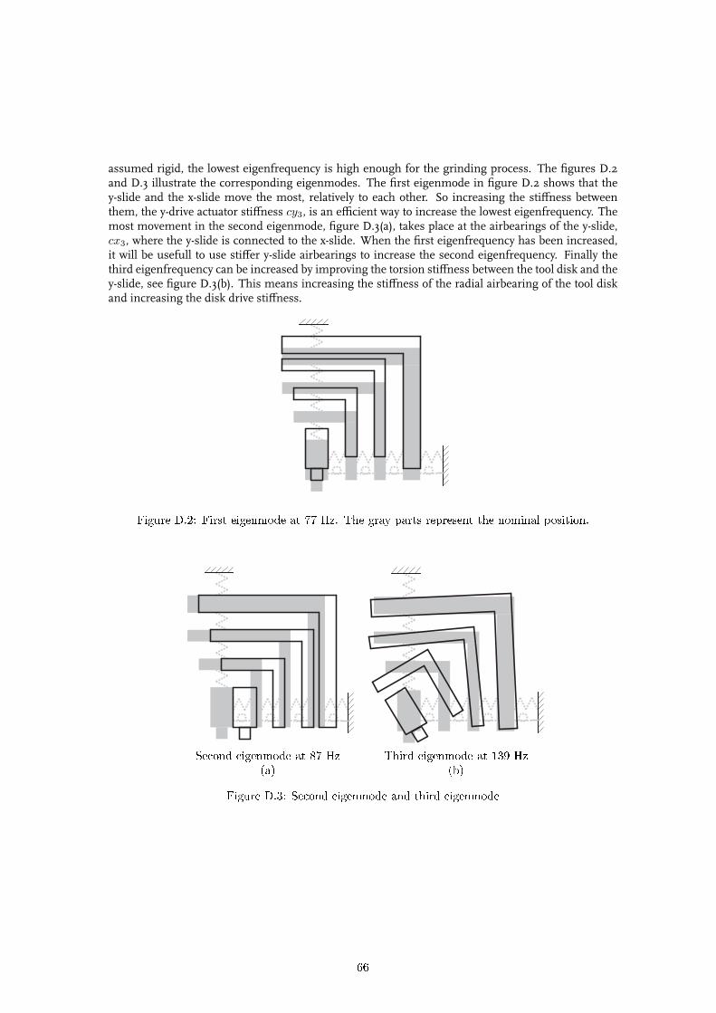
assumed rigid, the lowest eigenfrequency is high enough for the grinding process. The figures D.2and D.3 illustrate the corresponding eigenmodes. The first eigenmode in figure D.2 shows that they-slide and the x-slide move the most, relatively to each other. So increasing the stiffness betweenthem, the y-drive actuator stiffness cy3, is an efficient way to increase the lowest eigenfrequency. Themost movement in the second eigenmode, figure D.3(a), takes place at the airbearings of the y-slide,cx3, where the y-slide is connected to the x-slide. When the first eigenfrequency has been increased,it will be usefull to use stiffer y-slide airbearings to increase the second eigenfrequency. Finally thethird eigenfrequency can be increased by improving the torsion stiffness between the tool disk and they-slide, see figure D.3(b). This means increasing the stiffness of the radial airbearing of the tool diskand increasing the disk drive stiffness.

Figure D.2: First eigenmode at 77 Hz. The gray parts represent the nominal position.

Second eigenmode at 87 Hz Third eigenmode at 139 Hz(a) (b)

Figure D.3: Second eigenmode and third eigenmode

66

Appendix E

FEM-calculations

E.1 Introduction

After the global model of the entire grinder made in appendix D, some critical machine parts havebeen modeled with Finite Element Method. This way a more accurate dynamical behavior of themachine parts can be acquired. These models are also used to check wether the assumptions used inthe dynamical model of appendix D are correct.

E.2 X-frame

A FEM-calculation is made for the frame of the x-slide to determine the stiffness and the get an insightof the level of stress inside the frame. In figure E.1 the von Mises stress is given. A force is appliedon the centre line of the frame, where the y-slide drive is placed. The bottom side of the figure, wherethe airbearings to the vertical granite slab would be, is set as a fixed boundary condition. Because ofthe small process forces, the stresses on the frame are low. There is no risk of fatigue or exceedingthe yield strength of the aluminum. The figure gives an insight on how the stress is divided over theframe. The exact value is not really important. The figure shows that the stress is equal on most ofthe frame, except for a few areas. The highest stress is in the middle of the figure on the centre lineof the top plate. By moving this point as close as possible to the bottom side of the figure, the stressis reduced. More movement is not possible, because else the top plate would interfere with the toolspindle. When looking at the displacement of the point where the force is applied, the stiffness iny-direction can be determined. The y-stiffness of the x-frame is 3.3 · 108N/m.

Also the dynamical behavior of the frame is examined. Figures E.2 - E.4 show that the three lowesteigenfrequencies are at 257 Hz, 462 Hz and 582 Hz. The corresponding eigenmodes are also given.Because these eigenfrequencies are much higher than the lowest eigenfrequenties of the dynamicalmodel of appendix D, the dynamics of the x-frame do not play a significant role in the dynamics of theentire grinder.

E.3 Vacuum seal

The vacuum seal used to seal the top of the tool disk is examined more closely. A thin sheet thatis fixed axially to a mounting ring must prevent the atmospheric pressure to deform the seal radially.Because of the limited height of the tool disk it is not possible to use the shape of a semi-sphere for thesheet. Therefor a shape is used, using two curvatures, as shown in figure E.5. The curvature with R1

starts at the mounting ring in axial direction. This curvature is tangentially connected to the secondcurvature with R2, to prevent a large increase in stress on the border. The stress levels are given infigure E.6. A small increase in stress is showing at the border between the two curvatures. Because of

67

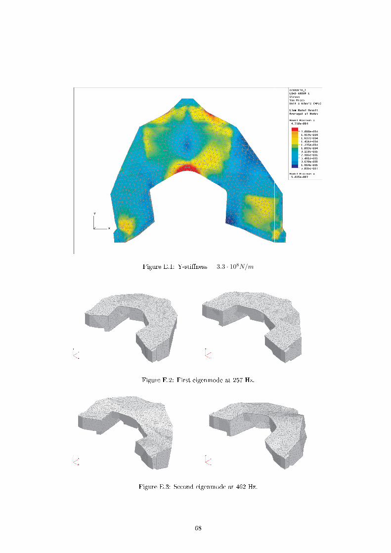
Figure E.1: Y-sti�ness = 3.3 · 108N/m

Figure E.2: First eigenmode at 257 Hz.

Figure E.3: Second eigenmode at 462 Hz.

68

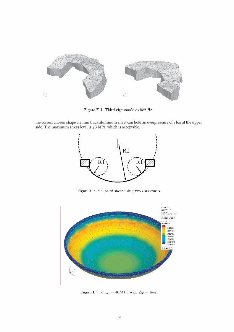
Figure E.4: Third eigenmode at 582 Hz.

the correct chosen shape a 2 mm thick aluminum sheet can hold an overpressure of 1 bar at the upperside. The maximum stress level is 46 MPa, which is acceptable.

Figure E.5: Shape of sheet using two curvatures

Figure E.6: σmax = 46MPa with ∆p = 1bar

69

E.4 Membranes

When the outer and inner ring of the membrane are exactly axially aligned, the radial stiffness of themembrane is very high, crad,max = 38 · 107N/m. However due to manufacturing tolerances this willnever be the case. There will always be some amount of axial offset. FEM-calculations are made toinvestigate the radial and axial stiffness of the membranes at an axial offset. Figure E.7 shows themaximum stress of 8 MPa when an axial offset of 0.01 mm is applied. This level is acceptable for thesteel membrane, so why not allow a larger axial offset? The radial stiffness is reduced from crad,max =38 · 107N/m to crad = 0.9 · 107N/m. A larger increase in offset will result in an unacceptable lowradial stiffness. The local axial stiffness - at the offset of 0.01 mm - is 5.3 · 103N/m. The force on thetool drive caused by the stiffness of the two membranes is little more than 0.05 N for a 10 µm stroke.

Figure E.7: Membrane: cax = 5.3 · 103N/m, crad = 0.9 · 107N/m, σmax = 8.0MPa

E.5 X-frame airbearings

To assure a proper working airbearing, the bottom side of the bearing, as described in 6.7, should beflat enough even when the air is flowing through. Because the airbearings surfaces on the edge ofthe bottom side are pushing the airbearing of the ground, and the vacuum chamber compensates thisforce by pulling the bearing down, a momentum on the air bearing is applied. This will cause theairbearing to bend, looking form the short side. Therefor six high plates are applied parallel to theshort side. These plates are very suited to prevent the momentum to cause a lot of deflection. Thisdeflection can cause the bottom side of the bearing to be convex, this will reduce the bearing stiffnessand increases the change of the bearing running into the under laying surface. Figure E.8 shows thestress levels in the airbearing. The increase in stress at the top middle of the six high plates show theneed for these plates. The flatness of the airbearing at the bottom side is 0.84µm, which is sufficientfor the 5µm air gape.

70

Figure E.8: Stresses on airbearing during air�ow

71

Appendix F

Calculations

F.1 Sti�ness related to overhanging length

When a body, as shown in figure F.1, is suspended on two spring with stiffness c, the deflection of thepoint on which the force F is acting is increased if F is not between the two springs. The distancebetween the two springs is L and the overhanging length is a. The two springs can be replaced by asingle spring with stiffness ct at the position of F . Figure F.2 shows the decrease in relative stiffnesswith an increase in overhanging length a. It shows the importance to minimize a in order to keep astiff construction. The curve in figure F.2 can be calculated with

ct

c= 1/(2

a

L

2+ 2

a

L+ 1) (F.1)

F

c c c t

a L

Figure F.1: Force applied on body at distance a from nearest suspension

F.2 Tool spindle accuracy model

To investigate if the desired accuracy can be produced, a simple model is made using the methode asdescribed in [TUe03]. Because of the partly parallel structural loop, a kinematic model can be made asshown in figure F.3. It shows a schematic view of the tool spindle unit. The movement the disk canmake on the granite base is represented by slide a. The movement made by the tool drive and rotoris represented by slide b. The distance between the two slides is c in z-direction and d in y-direction.

72

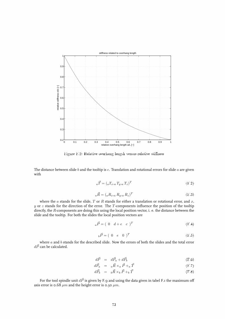
0 0.1 0.2 0.3 0.4 0.5 0.6 0.7 0.8 0.9 10.2

0.3

0.4

0.5

0.6

0.7

0.8

0.9

1

relative overhang length a/L [−]

rela

tive

stiff

ness

ct/c

[−]

stiffness related to overhang length

Figure F.2: Relative overhang length versus relative sti�ness

The distance between slide b and the tooltip is e. Translation and rotational errors for slide a are givenwith

a~T = (aTx,a Ty,a Tz)T (F.2)

a~R = (aRx,a Ry,a Rz)T (F.3)

where the a stands for the slide, T or R stands for either a translation or rotational error, and x,y or z stands for the direction of the error. The T -components influence the position of the tooltipdirectly, the R-components are doing this using the local position vector, i. e. the distance between theslide and the tooltip. For both the slides the local position vectors are

a~P = ( 0 d + e c )T (F.4)

b~P = ( 0 e 0 )T (F.5)

where a and b stands for the described slide. Now the errors of both the slides and the total errord~P can be calculated.

d~P = d~Pa + d~Pb (F.6)d~Pa = a

~R×a~P +a

~T (F.7)d~Pb = b

~R×b~P +b

~T (F.8)For the tool spindle unit d~P is given by F.9 and using the data given in tabel F.1 the maximum off

axis error is 0.68 µm and the height error is 0.30 µm.

73

d

c

a

b

e

y z

Figure F.3: Accuracy model

d~P =

aRy · c−a Rz · (d + e) +a Tx −b Rz · e +b Tx = 141 + 66 + 85 + 130 + 100−aRx · c +a Ty +b Ty = 141 + 85 + 74

aRx · (d + e) +a Tz +b Rx · e +b Tz = 146 + 50 + 133 + 100

(F.9)

74

Error Description Size [nm] or [µrad]aTx Position error of y-slide (35) + radial disk airbearing error (50) 85aTy Position error of y-slide (35) + radial disk airbearing error (50) 85aTz Axial disk airbearing error 50aRx Tilting caused by non-horizontal granite base 0.66aRy Tilting caused by non-horizontal granite base 0.66aRz Rotational error y-slide + accuracy angle measurement system 0.30bTx Tooltip runout error relative to the spindle stator 100bTy Tooltip runout error relative to the spindle stator 100bTz Tool length change due to temperature change 150bRx Tilt of tool drive in stator 1.0bRy Zero because of rotating tool 0bRz Tilt of tool drive in stator 1.0

Table F.1: Errors used in accuracy model

75

Appendix G

Alternative machine designs

G.1 Alternative 1

The first alternative machine design features a hydrostatic x-guideway, similar to the one on the Pre-citech Nanoform, see figure G.1. The guideway is rotated 90o compared to the normal way of mount-ing such a guideway. This way the guideway has got its highest stiffness in y-direction and this in-creases the process structural loop stiffness. Because the guideway consists of one solid piece it cannot be placed at workpiece spindle level centered on the workpiece. Therefor the guideway is placedat the front side of the horizontal granite slab. This leaves a lot of open space near the workpiece, butthis makes the position of the tool spindle very sensitive for tilting of the guideway in Rz, because ofthe long distance between the guideway and the workpiece. Also part of the y-direction stiffness is lostbecause the y-slide drive force is not applied at the centre line of the guideway. If the y-slide is actuateda momentum is created on the guideway in Rx-direction. The tool spindle disk uses an axial airbearingpreloaded with underpressure. Because of the sensitivity for guideway tilt and the only partly increasein y-stiffness this alternative was dismissed.

1. tool spindle 3. x-slide2. y-slide 4. hydrostatic guideway

Figure G.1: Alternative 1

76

G.2 Alternative 2

By mounting the hydrostatic guideway in a traditional way, the distance between the y-slide drive forceand the y-direction bearings of the x-slide is decreased and thus reducing the created momentum, seefigure G.2. However the highest stiffness of the guideway is used in the z-direction, so this alternativealso does not make advantage of the guideways full potential. The tool spindle disk is preloaded withtwo brackets that are connected to the y-slide. They press through the y-slide onto the tool spindledisk. This way the brackets do not have to rotate, only translate in x- and y-direction. The brackets arealso supported at the bottom of the horizontal granite slab, directly beneath the connection points onthe y-slide. This way only a force is applied on the slab and not a momentum. The bottom of the slabshould be flat and smooth enough to function as a bearing surface. Because of the high preload force(≈ 5000 N) needed to get a stiff bearing, large and heavy brackets are needed and this mass is movingwith the relative fast y-slide. So this will have its negative influence on the dynamics.

1. tool spindle disk 3. x-slide2. y-slide 4. preload bracket

Figure G.2: Alternative 2

Figure G.3 and G.4 show the tool spindle disk that is suspended with an hydrostatic oil bearing.Oil bearings can operate with a larger gap than airbearings, 30 µm instead of 5 µm. The appliedpressure of about 70 bar is much higher than the 5 or 6 bar with airbearings, resulting in smallerbearings. However, because of the larger gap, the preload force has to be larger. [Row83] showed thatthe stiffness of an hydrostatic bearing is given by

77

c = C · ps ·Ah

(G.1)C is a constant depending on the shape of the bearing and the restriction used, ps is the supply

pressure, A the bearing surface and h the gap height. Figure G.3 shows the disk on which the toolspindle will be mounted (1). On the edge of this disk slots are made (2), so bolts may be placed inthe underlaying holes. Also the radial oil bearing pockets are shown (3). Figure G.4 shows the axialoil bearing pockets (1). There are six pockets at the bottom to provide tilting stiffness to the disk. Therestriction (2) consists of a very narrow hole and a larger threaded hole. A bolt may be placed in thethreaded hole to act as a restriction. This way the flow of oil through the bearings, both the axial andthe radial bearings, can be adjusted. This way the bearing performance can be optimized. The oil flowenters the disk at the central oil canal (4) and is then divided into different oil canals (3) to each of thebearing pockets.

1. tool spindle mounting face 3. radial bearing pocket2. slots for adjustment screws

Figure G.3: Tool disk with hydrostatic bearing, isometric view

1. axial bearing pocket 3. oil canal2. restrictor 4. central oil canal

Figure G.4: Tool disk with hydrostatic bearing, section view

78

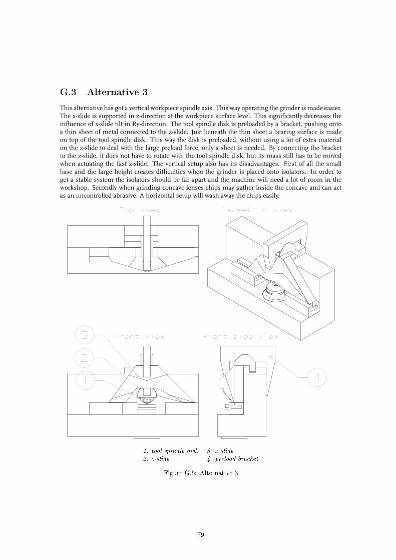
G.3 Alternative 3

This alternative has got a vertical workpiece spindle axis. This way operating the grinder is made easier.The x-slide is supported in z-direction at the workpiece surface level. This significantly decreases theinfluence of x-slide tilt in Ry-direction. The tool spindle disk is preloaded by a bracket, pushing ontoa thin sheet of metal connected to the z-slide. Just beneath the thin sheet a bearing surface is madeon top of the tool spindle disk. This way the disk is preloaded, without using a lot of extra materialon the z-slide to deal with the large preload force, only a sheet is needed. By connecting the bracketto the z-slide, it does not have to rotate with the tool spindle disk, but its mass still has to be movedwhen actuating the fast z-slide. The vertical setup also has its disadvantages. First of all the smallbase and the large height creates difficulties when the grinder is placed onto isolators. In order toget a stable system the isolators should be far apart and the machine will need a lot of room in theworkshop. Secondly when grinding concave lenses chips may gather inside the concave and can actas an uncontrolled abrasive. A horizontal setup will wash away the chips easily.

1. tool spindle disk 3. x-slide2. z-slide 4. preload bracket

Figure G.5: Alternative 3

79

G.4 Alternative spindle design

G.4.1 Alternative spindle design 1

This alternative spindle design features the second spindle concept, the one that uses an aerostaticbearing for the tool drive, see chapter 5. Figure G.6 shows the air spindle stator consisting of threeelements. On the outside there are two rings, that house the front and back airbearing surfaces, and inthe middle there is the motor stator. This way the front and back airbearing are far apart, so the rotorhas high tilting stiffness. And because the space between the two ring bearings is filled by the motor,room is spared. Also disturbing radial forces of the motor can be properly dealt with by both bearings.If the motor was placed at the back of the stator the disturbing radial forces would have caused thesame situation as described in F.2 and the bearings could have provided far less stiffness to resist theradial forces. The voice coil is placed at the back on the centre line. The stator is placed inside the toolspindle holder, completing the unit. The three stator parts should be aligned very well to prevent therotor from running into the stator at the airbearing surfaces.

1. tool spindle holder 4. motor2. front air bearing 5. voice coil3. back air bearing

Figure G.6: Alternative spindle design 1: aerostatic tool drive bearing

G.4.2 Alternative spindle design 2

This alternative spindle design has got the entire voice coil inside the rotor. Figure G.7 shows therotor of the tool spindle. A large bore provides space for the tool drive. The tool drive is suspendedto the rotor with two membranes. At the back of the tool drive the voice coil is placed. This setupneeds no extra space behind the rotor for the tool drive actuator, resulting in a smaller tool spindle.However this concepts features some difficulties. To get the required electrical current to the coil, aconnection with the fixed world is needed. The possibility of a slip ring has been investigated. There

80

are very few slip rings available that are suited for speeds up to 7000 rpm. These rings have a smalldiameter, to reduce the peripheral velocity. Because of this, such a ring can not be mounted laterallyto the rotor, so extra space is needed at the back of the rotor. The physical contact between the slipring rotor and stator introduces the problem of wear. The investigated slip ring has got a life spanof 100 · 10 6 revolutions. This means that when operating the grinder 40 hours per week at 5000rpm, the slip ring has to be replaced every two months. Also a slip ring introduces electrical noise thatmay influence the performance of the voice coil. This influence should be investigated, adding morecomplexity to a grinding experiment.

1 2 3 4

5

6

1. tool drive 4. slip ring2. membranes 5. rotor3. coil 6. motor rotor

Figure G.7: Alternative spindle design 2: using a slip ring

81

Appendix H

Materials

H.1 Optical materials

Material E [GPa] K [MPa/√

(m)] H [GPa] dc [nm]BK7 81 0.86 5.2 64Fused silica 73 0.75 5.6 35Soda-lime 72 0.7 5.9 25

Table H.1: Properties of materials used for optical componentsHere some properties of a number of glasses are given. Shown are the Youngs modulus E, the

toughness K and the hardness H . Also the critical depth of cut dc is given. A small dc means abrittle material. For the greater part, brittle material behavior is caused by a high hardness and a lowtoughness.

A commonly used material for optical components is BK7. The way of giving material such aname was first developed by Schott, Germany. The B stands for borosilicate. The K means it is acrown glass and this gives a certain range of values for the two most important optical properties ofthe material, namely the refractive index, nd and the Abbe number, νd. The refractive index nd givesthe refractive power of the glass relative to air, which has a nd of 1. The Abbe number νd is a measurefor the dispersion of the material, i.e. the difference in refraction for different wavelengths. For crownglass those properties are nd > 1.60 and νd > 50, or nd < 1.60 and νd > 55. Finally the number 7 ofBK7 means it is the seventh material developed in its category, [Kar93].

82

Appendix I

Data sheets

This appendix contains the data sheets of some of the components used in the grinder design. Thereare datasheets of the voice coil, the Blockhead air spindle used for the tool spindle, the Lion Precisioninductive measurement system, the granite used for the machine base, the environment isolators andthe Nanogrid measurement system.

83

Figure I.1: Voice coil datasheet84

Figure I.2: Tool spindle datasheet

85

ECL100 Linear OutputEddy Current Driver

Performance• Non-Linearity: ±0.25%FS• Resolution: 0.004%FS• Temp. Coeffi cient: 0.04%FS/°C• Frequency Response to 80kHz• Output: 0-10VDC and 0-20mA

Features• Local and Remote Zero• 12-24VDC Input• Range Indicating LEDs• Small DIN Rail Mounting• TEDS On Board• Synchronization of Multiple Units• User Calibration Adjustments

Precision displacement measurement; new, easy to use design.The ECL100 is small, easily mounted and provides the high performance levels you need in your application. It works with all Lion Precision Inductive probes with ranges from 0.5-15mm.

Core Unit

Smooth

Threaded

Bulkhead

Document LL02-0010 08-2004

563 Shoreview Park Rd.St. Paul, MN 55126651-484-6544www.lionprecision.com

LIONLIONPRECISIONPRECISION

Probes Choose from our four standard body styles:Core unit features the smallest physical size for limited access applications.Smooth body has the strength of a stainless steel housing for clamp or set screw mounting and easy adjustment of axial position.Threaded body provides a threaded, stainless steel housing for precise adjustment of axial position in a threaded mounting hole or a through hole using the two lock nuts provided.Bulkhead body’s fl anged, stainless steel housing gives you easy axial position repeatability in a threaded or through hole.

Custom ProbesAll body styles are built from the same core unit. Custom body styles are turned around quickly to get you up and running with exactly what you need in your application.

Figure I.3: Inductive measurement datasheet 1/2

86

ECL100 Driver Specifi cations:*Resolution:RMS @ mid-scale

DC-1kHz 0.004%FS

DC-10kHz 0.008%FS

DC-80kHz 0.06%FS

Non-linearity ±0.25%FS

Probe Temperature Coeffi cient ±0.04%FS/°C(±0.05%FS/°C for U3)

from -25°C to +125°C†

output @ mid-scale

Driver Input Power +12 to +24VDC130mA @ 15V

Driver Outputs Voltage 0-10VDC

Current 0-20mA

Operating Temperature:

Std. Probes -25°C to +125°C†

Ext. Temp. Probes -25°C to +200°C†

Driver 0°C to +65°C

Probe Cables Length 3 meters

Jacket Material Std. Temp. PUR

Ext. Temp. TEFLON

Ratings Driver IP40 (CE Pending)

Probes Std.. Temp. - IP67Ext. Temp. - IP63

Driver Dimensions Height 75mm / 2.95"

Width 22.5mm / 0.89"

Depth 107.5mm / 4.23"

Weight 103g / 3.7oz.

* Performance data taken with standard unshielded probes, 15VDC input, normal room ambient, 6061 aluminum target. Specs also apply to 4140 and 303 steels.† Probes available to less than -75°C with special calibration

75m

m2.

95"

22.5mm0.89"

107.5mm4.23"

TEDSNCGround+15 VDC In

Red - NearGreen - 0-20%FS

Green - 20-80%FS

Green - 80-100%FSRed - Far

V Out (0-10 VDC)V GroundI Out (4-20 mA)I Ground

35mm

7.5mm

ECL100 Driver Mounts to standard EN 50 022 symmetrical mounting rail.

Probe Dimensions

AX

mm/inchY

mm/inch B XY

mm/inch

— — — U3B M3x.5 21.1/0.83

U5A 3.4/0.13 13.0/0.51 U5B M5x.8 25.0/0.99

U8A 6.2/0.24 14.0/0.55 U8B M8x1 27.0/1.07

U12A 10.0/0.39 15.0/0.59 U12B M12x1 29.0/1.15

U18A 15.8/0.62 16.0/0.63 U18B M18x1 31.0/1.22

— — — U25B 25.0/0.99 15.0/0.59

— — — U38B 38.0/1.50 20.0/0.79

— — — U50B 50.0/1.97 25.0/0.99

CX

mm/inchY

mm/inch DX

threadY

mm/inch

U3CShoulder

2.92/0.1153.6/0.14

16/0.635/0.20

— — —

U5C 4.9/0.193 21/0.83 U5D M5x.8 23/0.91

U8C 7.9/0.311 23/0.91 U8D M8x1 25/0.99

U12C 11.9/0.468 25/0.99 U12D M12x1 27/1.07

U18C 17.9/0.705 27/1.07 U18D M18x1 31/1.22

Probe Range and Resolution:*

Probe Model

Rangemm/inch

Offsetmm/inch

Resolutionµm/µinch

1kHz 10kHz 80kHz

U3 0.50/0.020 0.05/0.002 0.02/0.8 0.04/1.6 0.30/13

U5 1.25/0.050 0.25/0.010 0.05/2 0.10/4 0.75/30

U8 2.00/0.080 0.35/0.015 0.08/3 0.16/6 1.20/48

U12 3.50/0.140 0.60/0.025 0.14/6 0.28/11 2.10/84

U18 5.00/0.200 0.75/0.030 0.20/8 0.41/16 3.05/120

U25 8.00/0.320 1.25/0.050 0.28/11 0.57/22 4.88/192

U38 12.5/0.500 1.50/0.060 0.48/19 0.96/38 7.16/282

U50 15.0/0.600 2.00/0.080 0.66/26 1.32/52 9.91/390

*Specifi cations for 6061 aluminum and 4140 steel. Other ferrous and nonferrous materials will produce similar results.

Y

XA

Y

XC

Y

XD

Y

XB U3-U18

Y

M18 x 1

28mm/1.1"

X

B U25-U50

563 Shoreview Park Rd.St. Paul, MN 55126651-484-6544www.lionprecision.com

LIONLIONPRECISIONPRECISION

Figure I.4: Inductive measurement datasheet 2/2

87

DATASHEET

MATERIAL PROPERTIES

...1 / 1 …

Granite Precision Engineering

BoTech

BoTech BV – PO Box 6052, 5700 ET Helmond (NL) - Korte Dijk 2, 5705 CV Helmond (NL) -Tel: (+31)492–55 18 75 - Fax:(+31) 492–52 76 35 – info@botechbv.com - www.botechbv.com

Can be delivered by BoTech BV:

Von BoTech BV lieferbar / Door BoTech BV leverbaar:

Granite Silicate Ceramics

Granit / Graniet Silikat-Keramik / Silicaat Keramiek

Properties for

comparison only

Nur als

Vergleichswerte / Waarden ter vergelijking

Table for Comparison Vergleichstabelle / Vergelijkingstabel

Impa

la*

Afr

ican

Bla

ck*

Afrik

a Sc

hwar

z / A

frik

a Zw

art

Type

C

Type

D

Al 2O

3 (9

2)

Al

Wasseraufname / Waterabsorptie

Water absorption [ % ] 0,2 – 0,4 0,2 – 0,4 0,0 0,0 0,0 0,0

Rohdichte / Dichtheid

Specific Gravity [ 103 kg/m3 ] 2,9 3,1 2,2 3,2 3,6 2,7

Biegefestigkeit / Buigsterkte

Flexural Strength [ N / mm2 ] 13 5 - 10 80 250 240 170

Elastizitätsmodul / Elasticiteitsmodulus

Modulus Of Elasticity [ 103 N/mm2 ] 65 - 85 77 80 200 300 69

Druckfestigkeit / Druksterkte

Compressive Strength [ N / mm2 ] 240 200-300 400 1000 3000 65-200

Lin. Längenausdehnungskoeffizient / Lineaire Uitzettingscoëfficiënt Coefficient Of Linear Thermal Expansion

[ 10-6 K-1 ]

(20 – 100 °C) 5-6 4-7 0,4 5 - 7 7 23

Spezifische Wärmekapzität / Soortelijke Warmte

Specific Heat [ J / kg.K ]

(20 – 100 °C)

800 800 - 950 960 960

Wärmeleitfähigkeit / Thermische warmtegeleidingscoëfficiënt

Thermal Conductivity [ W / m.K ] 3,2 2,9-3,5 2 12 21 171

*Values must be seen as indications. (Small) variations in composition lead to variations in properties of this natural product. *Angegebene Werte sind Richtzahlen. (Geringe) Variationen in der Zusammenstellung führen zu Variationen in den Materialeigenschaften von diesem Naturprodukt.

*Weergegeven waarden zijn richtgetallen. (Geringe) variaties in samenstelling leiden tot variaties in de materiaaleigenschappen van dit natuurprodukt.

Also available:

Datasheet Impala Datasheet African Black Datasheet Carbon Fibre / Epoxy Composites

TABLE FOR COMPARISONVergleichstabelle / Vergelijkingstabel

Figure I.5: Granite datasheet

88

1248

OPTI

CAL T

ABLE

SBR

EADB

OARD

S &

GRID

PLAT

FORM

SHO

NEYC

OMB,

GRA

NITE

&RI

GID

STRU

CTUR

ESIS

OLAT

ORS

WOR

KSTA

TION

S &

ISOL

ATED

PLA

TFOR

MS

STRU

CTUR

AL R

AILS

&CA

RRIE

RSTE

STIN

G, A

NALY

SIS

& DE

SIGN

TECH

NICA

L REF

EREN

CE

I-2000 LabLegs™

Stabilizer Pneumatic IsolatorsWith Automatic Leveling

I-2000 Stabilizer™ vibrationisolators offer a vibration isolationdesign that has set the standard inperformance and convenience.

Exclusive laminar flow damping isthe heart of the Stabilizer’sunparalleled performance. Unlikesingle damping orifices, the Stabilizeremploys thousands of tiny orifices,resulting in greater dampingefficiency overall. Combined with thehybrid chamber design to minimizeair volume between piston motionand damper air flow, the Stabilizerprotects applications like no other.

Numerous performance advantagesinclude:

• Faster settling time for large andsmall magnitude disturbances.

• Greater high-center-of-massstability—a must for heavyequipment.

• Lower natural frequency for superiorprotection against hard-to-controllow frequencies below 5 Hz.

Installation is fast and easy withpatented, self-centering pistons. Theyautomatically center the piston at thetop and bottom of its vertical stoke,guaranteeing unrestricted movementfor optimal performance. SafeLock™mounting brackets eliminate the needto precisely align isolators and tableholes when attaching the isolator tothe table.

I-4000 isolators are available from the CustomProducts Group

Key Features

Hybrid Chamber Design• Maximized isolation bandwidth

• Improved center of mass stability

• Better responsiveness

• Compact design

Laminar Flow Damping• Less amplification at resonance

• Better isolation bandwidth

• Improved settling time

High Accuracy Leveling Valves• Improved repositioning after

disturbance

• Better beam pointing stability

• User control of airflow

Trifilar Pendulum Horizontal Isolation• Zero-friction for isolation of very low

level vibration

• Excellent damping properties

Tie-Bar System

Tie-Bar Caster System

• Minimized amplification atresonance, thereby maximizing thesystem’s stability overall.

Figure I.6: Isolator datasheet 1/2

89

1249Email: sales@newport.com • Web: www.newport.com

TECHNICAL REFERENCETESTING, ANALYSIS

& DESIGNSTRUCTURAL RAILS &

CARRIERSW

ORKSTATIONS &ISOLATED PLATFORM

SISOLATORS

HONEYCOMB, GRANITE &

RIGID STRUCTURESBREADBOARDS & GRID

PLATFORMS

OPTICAL TABLES

Specifications

Isolation Specifications

Model

Vertical Isolation* Horizontal Isolation*Amplificationat Resonance Damping

ElementAirflow

Horz.Damping

Load perIsolator[lb (kg)]

Res(Hz)

5Hz(%)

10Hz(%)

Res(Hz)

5Hz(%)

10Hz(%)

Vert(dB)

Horz(dB)

I-2000 Series 1 96 99 1.5 85 95 13 13 Normal Oil 2000 (900)

* Isolation at full load

Physical Specifications

Height [in. (mm)] 10 (254), 13.5 (343), 16 (406), 19.5 (495), 22 (559), 23.5 (597), 28 (711)Height Adjustment [in. (mm)] 1.3 (33)Valve IPV-S1Re-leveling Accuracy [in. (mm)] ±0.010 (±.250)Settling Time 1.5 sec. (typical)Max. Air Pressure [psi (kg/cm2)] 20–85 (0.7–6.0)Self Centering Yes

Ordering Information

Order using this general format:

I-2000-NH

Number ofIsolators per set

Isolator height (inches)

Tie-Bar/Caster System Options

Standard tie-bar/caster systems areavailable for the table sizes listedbelow. Select from the Modelnumbers below to add a standardload tie-bar system—with or withoutcasters—to your table. For othertable sizes, please contact Newportfor price and delivery.

Tie-Bars with CastersTables[ft (m)] Model (Metric)

4 (1.2) x 6 (1.8) TBC-46 (M-TBC-46)4 (1.2) x 8 (2.4) TBC-48 (M-TBC-48)4 (1.2) x 10 (3.0) TBC-410 (M-TBC-410)4 (1.2) x 12 (3.6) TBC-412 (M-TBC-412)5 (1.5) x 6 (1.8) TBC-56 (M-TBC-56)5 (1.5) x 8 (2.4) TBC-58 (M-TBC-58)5 (1.5) x 10 (3.0) TBC-510 (M-TBC-510)5 (1.5) x 12 (3.6) TBC-512 (M-TBC-512)

Tie-Bars onlyTables[ft (m)] Model (Metric)

4 (1.2) x 6 (1.8) TB-46 (M-TB-46)4 (1.2) x 8 (2.4) TB-48 (M-TB-48)4 (1.2) x 10 (3.0) TB-410 (M-TB-410)4 (1.2) x 12 (3.6) TB-412 (M-TB-412)5 (1.5) x 6 (1.8) TB-56 (M-TB-56)5 (1.5) x 8 (2.4) TB-58 (M-TB-58)5 (1.5) x 10 (3.0) TB-510 (M-TB-510)5 (1.5) x 12 (3.6) TB-512 (M-TB-512)

Vertical

0.8 10 30

TR

AN

SM

ISS

IBIL

ITY

10

1

0.1

0.01

0.001

VERTICAL FREQUENCY (Hz)

20

0

dB

-20

-40

-60

Horizontal

HORIZONTAL FREQUENCY (Hz)300.8 10

TR

AN

SM

ISS

IBIL

ITY

10

1

0.1

0.01

0.001

20

0

dB

-20

-40

-60

ø 6.75 (171).19 (4.8)

1.3 (33)HEIGHT ADJUST.

±.25 (6)TRAVEL

ø 10.00 (254.0)

h

H

Other heights available upon request

Dimension [in. (mm)]Model H hI-2000-N10 10.0 (254) N/A

I-2000-N13.5 13.5 (343) 1.7 (43.2)

I-2000-N16 16.0 (406) 3.8 (96.5)

I-2000-N19.5 19.5 (495) 7.3 (185.4)

I-2000-N22 22.0 (559) 9.8 (248.9)

I-2000-N23.5 23.5 (597) 11.3 (287.0)

I-2000-N28 28.0 (711) 15.8 (401.3)

Other heights available upon request

Example: I-2000-428 designates asystem with four 28 in. isolators. Toadd a tie-bar caster system for a 4 ft x8 ft table, add -TC after the Modelnumber and order tie-bars and/orcasters as below:

1) I-2000-428-TC

2) TBC-48

Model Number of IsolatorsLoad Capacity

[lb (kg)]I-2000-4H 4 660 (300)–8000 (3640)I-2000-6H 6 990 (450)–12000 (5455)I-2000-8H 8 1320 (600)–16000 (7280)

Figure I.7: Isolator datasheet 2/2

90

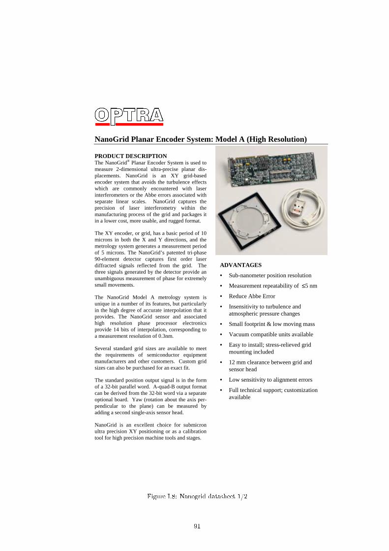
NanoGrid Planar Encoder System: Model A (High Resolution) PRODUCT DESCRIPTION The NanoGrid® Planar Encoder System is used to measure 2-dimensional ultra-precise planar dis-placements. NanoGrid is an XY grid-based encoder system that avoids the turbulence effects which are commonly encountered with laser interferometers or the Abbe errors associated with separate linear scales. NanoGrid captures the precision of laser interferometry within the manufacturing process of the grid and packages it in a lower cost, more usable, and rugged format.

The XY encoder, or grid, has a basic period of 10 microns in both the X and Y directions, and the metrology system generates a measurement period of 5 microns. The NanoGrid’s patented tri-phase 90-element detector captures first order laser diffracted signals reflected from the grid. The three signals generated by the detector provide an unambiguous measurement of phase for extremely small movements.

The NanoGrid Model A metrology system is unique in a number of its features, but particularly in the high degree of accurate interpolation that it provides. The NanoGrid sensor and associated high resolution phase processor electronics provide 14 bits of interpolation, corresponding to a measurement resolution of 0.3nm.

Several standard grid sizes are available to meet the requirements of semiconductor equipment manufacturers and other customers. Custom grid sizes can also be purchased for an exact fit.

The standard position output signal is in the form of a 32-bit parallel word. A-quad-B output format can be derived from the 32-bit word via a separate optional board. Yaw (rotation about the axis per-pendicular to the plane) can be measured by adding a second single-axis sensor head.

NanoGrid is an excellent choice for submicron ultra precision XY positioning or as a calibration tool for high precision machine tools and stages.

ADVANTAGES

• Sub-nanometer position resolution

• Measurement repeatability of ≤5 nm

• Reduce Abbe Error

• Insensitivity to turbulence and atmospheric pressure changes

• Small footprint & low moving mass

• Vacuum compatible units available

• Easy to install; stress-relieved grid mounting included

• 12 mm clearance between grid and sensor head

• Low sensitivity to alignment errors

• Full technical support; customization available

Figure I.8: Nanogrid datasheet 1/2

91

OPTRA, Inc. 461 Boston St. Topsfield, MA 01983 978-887-6600 FAX: 978-887-0022 NanoGrid A.doc info@optra.com or www.optra.com 7/20/2000

NanoGrid Model A (High Resolution)

TECHNICAL SPECIFICATIONS

System Performance

Repeatability ±5nm Accuracy (175mm×175mm)* ±200nm Accuracy (380mm×380mm)* ±1.0µm

* (Temperature stabilization to ±0.25°C) Maximum velocity 700mm/sec Encoder to sensor head gap 12.0 ±0.1 mm Measurement area (others available)

40×45mm, 150×150mm 210×210mm, 380×380mm

Operating temperature +10°C to +40°C Storage temperature –20°C to +50°C

NanoGrid Sensor Head Dimensions 23.5 × 47.0 × 60.5mm Housing material 6061-T6 aluminum Light source (785nm) Class IIIb 3mW laser diode Weight without cable 110gm Interface cable 3 m cable, 15-pin connector

Two-Axis High-Resolution Processor Resolution LSB = 5µm ÷ 214 ≈ 0.305 nm Update rate/axis (parallel out) 375 kHz Range ~1300 mm (32 bit rollover) Data age < 8µsec; stability < 25 nsec Interfaces 25-pin test connector

Two 60-pin parallel connectors PC-compatible 16-bit ISA bus

15-pin HD to Sensor Head Output format 32-bit parallel word (each axis) A-quad-B (optional) Edge rate: 1.875, 3.75, 7.5, 15MHz

Resolution: 5µm÷2N; N = 9 to 14; ≈0.3 to 9.8 nm

Edge-rate & resolution selectable Mechanical ISA-compatible 16-bit PC board Power (Does not include A-quad-B board)

+5VDC (+0.25/-0.13 V)@ 2.2 A; +12VDC ±0.5V @120 mA; –12VDC ± 0.5V @70 mA

NanoGrid Encoder

Pitch (mechanical/optical) 10 µm / 5µm Soda-lime expansion coefficient: 7.0 × 10-6/°C Quartz (fused silica) expansion coeff: 0.7 × 10-6/°C Other materials available – consult factory

System Components The NanoGrid Model A System consists of a planar encoder (XY grid), sensor head with cable, and 2-axis hi-resolution processor board.

NanoGrid Sensor Head The NanoGrid Sensor Head contains a single laser diode source and separate optical systems for making planar position measurements. Output signals from the Sensor Head go to the Processor.

Two-Axis High-Resolution Processor The Two-Axis High-Resolution Processor is a full size, ISA-bus-compatible PC plug-in card. It supplies power to, and receives signals from the NanoGrid Sensor Head via an interface cable. After processing these signals, it generates 32-bit words which describe the position of the encoder relative to the NanoGrid Sensor Head. Binary (TTL) flags and board-mounted LED’s indicate excess speed and low signal conditions. An optional daughter board provides an A-quad-B output with selectable resolution.

NanoGrid Encoder The standard NanoGrid encoder is a 10 µm pitch, 2-dim-ensional diffraction grating on soda-lime glass. The XY grid can be attached to a metal ring with incorporated flexures that provides kinematic KineFlex mounting with stress relief and ease of installation.

Documentation Package This package contains dimensional and tolerance inform-ation needed to properly locate the NanoGrid sensor head relative to the NanoGrid encoder, instructions for mount-ing the NanoGrid encoder, and an operating manual.

OPTRA and NanoGrid are registered trademarks and KineFlex is a trademark of OPTRA, Inc.

Figure I.9: Nanogrid datasheet 2/2

92