design methodology for multi-element high-lift … · design methodology for multi-element...
TRANSCRIPT
NASA-CR-202365 / . L
/
c"_ /._-
Design Methodology for Multi-Element High-Lift Systems on SubsonicCivil Transport Aircraft
R.S. Pepper and C.P. van DamDepartment of Mechanical and Aeronautical Engineering
University of CaliforniaDavis, CA 95616
Final Report
Cooperative Agreement NCC2-5042
August 1996
https://ntrs.nasa.gov/search.jsp?R=19960054343 2018-06-25T00:39:33+00:00Z

Abstract
The choice of high-lift system is crucial in the preliminary design process of a
subsonic civil transport aircraft. Its purpose is to increase the allowable aircraft weight or
decrease the aircraft's wing area for a given takeoff and landing performance. However,
the implementation of a high-lift system into a design must be done carefully, for it can
improve the aerodynamic performance of an aircraft but may also drastically increase the
aircraft empty weight. If designed properly, a high-lift system can improve the cost
effectiveness of an aircraft by increasing the payload weight for a given takeoff and
landing performance. This is why the design methodology for a high-lift system should
incorporate aerodynamic performance, weight, and cost.
The airframe industry has experienced rapid technological growth in recent years
which has ted to significant advances in high-lift systems. For this reason many existing
design methodologies have become obsolete since they are based on outdated low
Reynolds number wind-tunnel data and can no longer accurately predict the aerodynamic
characteristics or weight of current multi-element wings. Therefore, a new design
methodology has been created that reflects current aerodynamic, weight, and cost data
and provides enough flexibility to allow incorporation of new data when it becomes
available.
ii

This page intentionally left blank
iii

Table of Contents
Abstract ............................................................................................................................... ii
Acknowledgments .............................................................................................................. iii
Table of Contents ............................................................................................................... iv
List Of Figures ................................................................................................................... vi
Nomenclature ................................................................................................................... viii
1.0 Introduction .................................................................................................................... 1
2.0 High-Lift Configurations ............................................................................................... 4
2.1 Trailing-Edge Devices ................................................................................. 4
2.1.1 Plain Flaps .......................................................................................................... 5
2.1.2 Slotted Flaps ...................................................................................................... 5
2.1.3 Fowler Flaps ....................................................................................................... 7
2.2 Leading-Edge Devices ....................................................................................... 9
2.2.1 Slats .................................................................................................................. 10
2.2.2 Krager Flaps ..................................................................................................... 10
3.0 Performance Requirements .......................................................................................... 16
3.1 Takeoff ............................................................................................ 16
3.2 Landing ................................................................................................................... 18
4.0 Design Constraints ....................................................................................................... 21
5.0 Computational Modeling ............................................................................................. 24
" 26.0 Aerodynamic Database ........................................................................................ 6
7.0 Aerodynamic Module ......................................................................................... 33
7.1 Two-Dimensional Aerodynamics ........................................................................... 33
7.1.1 Lift .................................................................................................................... 34
7.1.2 Drag .................................................................................................................. 38
7.1.3 Pitching Moment .............................................................................................. 40
7.2 Three-Dimensional Aerodynamics .................................................................... 42
7.2.1 Lift .................................................................................................................... 44
iv

7.2.2 Drag .................................................................................................................. 45
7.2.3 Pitching Moment .............................................................................................. 46
7.3 Maximum Lift Prediction ....................................................................................... 46
7.3.1 Two-Dimensional ............................................................................................ 47
7.3.2 Three-Dimensional .......................................................................................... 49
8.0 Weight Module ............................................................................................................ 58
8.1 Trailing-Edge Flap Weight ..................................................................................... 59
8.2 Leading-Edge Flap Weight ..................................................................................... 61
9.0 Cost Module ................................................................................................................. 66
10.0 Sample Application .................................................................................................... 70
11.0 Concluding Remarks .................................................................................................. 82
References .......................................................................................................................... 85
Appendix A ........................................................................................................................ 89
Appendix B ........................................................................................................................ 96
V

List Of Figures
Figure 1.1
Figure 2.1
Figure 2.2
Figure 2.3
Figure 2.4
Figure 2.5a
Figure 2.5b
Figure 2.6
Figure 2.7
Figure 3.1
Figure 3.2
Figure 6.1
Figure 6.2
Figure 6.3
Figure 6.4
Figure 6.5
Figure 6.6
Figure 6.7
Figure 6.8
Overview of High-Lift Module Integration ........................................... 3
Lift Curves for Various High-Lift Airfoils .......................................... 12
Trailing-Edge Flap Configurations ...................................................... 12
High-Lift Support Types ...................................................................... 13
Definition of Fowler Action ................................................................. 13
Usable Lift of Civil Transport Aircraft ................................................ 14
Tail-Scrape Angle of a Typical Civil Transport Aircraft ..................... 14
Various Leading-Edge Devices ........................................................... 15
Surface Disturbances Created by Leading-Edge Devices
in Cruising Flight ................................................................................. 15
FAR 25 Takeoff Requirements ............................................................ 20
FAR 25 Landing Requirements ........................................................... 20
Two and Three-Element Airfoil Geometries ....................................... 28
Sample CHIMERA Grid of the NLR-7301Two-Element Airfoil ............................................................................ 28
NLR-7301 Pressure Distribution (or=6 °, Re=2.51 xl 06) ...................... 29
NLR-7301 Lift Curve (Re=2.51 x 10⁶) .................................................. 29
NLR-7301 Drag Polar (Re=2.51xl06) ................................................. 30
Sample CHIMERA Grid of the Douglas LB-546Three-Element Airfoil .......................................................................... 30
Douglas 3-Element Pressure Distribution
(ct=8.1 °, Re=9.0x 10⁶) ........................................................................... 31
Douglas 3-Element Lift Curve (Re=9.0xl 06) ...................................... 31
vi

Figure6.9
Figure7.1
Figure7.2
Figure7.3
Figure7.4
Figure7.5
Figure7.6
Figure7.7
Figure7.8
Figure7.9
Figure7.10
Figure7.11
Figure7.12
Figure8.1
Figure8.2
Figure10.1
Figure 10.2
Douglas3-ElementDragPolar(Re=9.0xl06)......................................32
NLR-7301SeparationFactor...............................................................51
- NLR-7301Lift-Effectiveness..............................................................51
- Overviewof AerodynamicAnalysis....................................................52
- Part-Span-FlapDeflectionTestCase...................................................53
- Part-Span-FlapSpanwiseLoadDistributionVTW7S1Configuration,a=l 1.4° ........................................................53
- Part-Span-FlapSpanwiseLoadDistributionVTW7 Configuration,a=8.5° ..............................................................54
- Swept-WingTestCase.........................................................................54
Swept-WingLift DistributionPlainWingModel, CL=0.4...................................................................55
Swept-WingLift DistributionCambered& TwistedWing Model,CL=0.4........................................55
Procedurefor CalculatingPitchingMoment.......................................56
IncrementIn StallAngleDueto VariousL. E.Devices......................56
MaximumLift EstimationUsingCritical SectionApproach..............................................................................................57
- Trailing-EdgeWeightCorrelationsfor VariousAircraft.....................65
- Leading-EdgeWeightCorrelationsfor VariousAircraft.....................65
- Lift Curvesof SampleTestCases........................................................81
- DragPolarsof SampleTestCases.......................................................81
vii

Nomenclature
(Z
al,2 ..... etc.
C_.8
(_0
AR
b 1,2 ..... etc.
c
Z
C
C 12 ..... etc.
CD
Cd
Cdmi n
CL
Ci
CL_
¢-_ clean"-'18
CIsma x
CLE/TE
Clmax
CLma x
Clmi n
Cm
CM
dl.2 ..... etc.
ACtmax
Ac
ACL
ACLm_x
_LE/TE
ASFowler
gw
f,
2,
angle of attack (rad)
empirical constants
lift-effectiveness of flap (O0_vz /
angle of attack at zero lift (rad)
aspect ratio of wing
empirical constants
reference cruise chord length in the streamwise direction (ft)
separation factor of flap
extended chord length due to system deployment (ft)
empirical constants
drag coefficient based on reference area
local drag coefficient based on local reference chord
minimum drag coefficient
lift coefficient of wing based on the reference arealocal lift coefficient based on the local reference chord
lift curve slope of wing (rad -l)
local lift curve slope of airfoil (rad -l)
local lift curve slope of cruise airfoil (rad -I)
lift-effectiveness of flap (rad -l)
maximum lift-effectiveness of flap (rad -1)
leading or trailing-edge device chord length (ft)
local maximum lift coefficient based on the reference chord
maximum lift coefficient of wing based on the reference area
lift coefficient at minimum drag
local pitching moment coefficient based on the local reference
chord
pitching moment coefficient of wing based on the reference area
empirical constants
change in stall angle due to deployed leading-edge device (rad)
increase in chord due to Fowler action (ft)
increment in lift (linear region) due to high-lift devices
maximum increment in lift due to high-lift devices
leading or trailing-edge device deflection angle (rad)
increase in flap area due to Fowler motion (ft2)
wing twist angle (rad)
l, owler action function of 1s, flap element
Fowler action function of 2"d flap element
flight-path angle of aircraft (rad)
viii

r] LE/TE
A
L
L/D
M
0
0tail-scrape
Re
S
St
$2
SLE
STEt/c
U/C
VI
V2
VA
VLOF
VMC
VMCC
VMS
VMU
VR
gslg
VTD
WE
X 1,2 ..... etc.
Xac
Xcp
leading/trailing-edge device span break locations (% of wing span)
profile drag polar constant
quarter chord sweep angle of wing (rad)
wing taper ratio
lift-to-drag ratio of wing
freestream Mach number based on V2 for takeoff and VA for
landing
fuselage angle (rad)
tail-scrape angle of fuselage (rad)
Reynolds number based on V2 for takeoff and VA for landing
wing reference area (ft2)
shroud length of main element
shroud length of 1s, flap element
planform area of leading edge flap (ft 2)
ptanform area of stowed flap (ft 2)maximum thickness ratio of cruise airfoil
landing gear
decision speed (kts)
takeoff climb speed (kts)
approach speed (kts)
lift-off speed (kts)
minimum control speed (kts)
minimum control speed on the ground (kts)
minimum dynamic stall speed (kts)
minimum unstick speed (kts)
rotation speed (kts)
stall speed of aircraft in steady flight (kts)
touch-down speed (kts)
maximum landing weight (lb)
empirical exponents
aerodynamic center of airfoil section (ft)
center of pressure of airfoil section (ft)
ix

1.0 Introduction
The design of an efficient high-lift system remains as challenging today as it was
twenty years ago when A.M.O. Smith wrote his enlightening papers on high-lift
aerodynamics.l,2 Modern civil transport aircraft require complex multi-element high-lift
systems to meet stringent performance criteria during the takeoff and landing phases of
flight. In the current competitive market place, new aircraft designs are driven to simpler,
more efficient high-lift systems that provide improved aerodynamic performance in terms
of increased maximum lift coefficient, Cr.,_, increased lift-to-drag ratio, L/D, or
increased lift coefficient, CL, for a given angle of attack and flap setting. Garner and his
co-workers at Boeing 3 present excellent examples illustrating the importance of a high-lift
system in the design of a B777 type of aircraft:
1. ACL=+0.10 for a constant angle of attack on approach for landing reduces the pitch
attitude angle by about one degree. For a given aircraft geometry and landing-gear
location this allows a reduction in landing-gear height and an associated weight
reduction of 1,400 lb.
2. AC Lmax = + 1.5 % at a fixed approach speed results in an increase in payload of
6,600 lb.
3. A(L/D)=+0.10% on takeoff results in an increase in payload of 2,800 lb.
These examples illustrate the enormous importance of a well designed and
engineered high-lift system in the overall development process of a subsonic civil
transport aircraft. However, these systems also increase the structural weight,
complexity, maintenance requirements, and cost of an aircraft. Thus, the designer is
faced with the task of developing such a high-lift system that allows the airplane to meet

thetakeoffandlandingperformancerequirementswhileminimizing theweightandcost
of theairplane.
Thisreportpresentsadesignmethodologyfor multi-elementhigh-lift systemsfor
subsoniccivil transportaircraftthatincludesaerodynamicperformance,structuralweight
considerations,systemcomplexity,andcost. Themethodologyis designedto be
compatiblewith ACSYNT4,amultidisciplinarycomputer-aidedaircraftconceptual
designtool. Consequently,importantconsiderationsare(I) to find areasonable
compromisebetweentheCPUrequirements(oncurrentgenerationworkstations)of the
high-lift moduleandtheaccuracyof thepredictionsby themoduleand(2) to provide
enoughflexibility to enhancethecapabilitiesof thehigh-lift modulewhenmorepowerful
hardwareandsoftwarebecomesavailable.
It is envisioned that this methodology will be integrated into ACSYNT as
illustrated in figure 1.1. Once the development of the aerodynamic database for double
and triple-slotted flaps is finished, the high-lift module can be used in the 1st level of
design as described in this report. Given the initial concept and mission requirements,
iteration is required to find the optimum initial high-lift configuration based on general,
or historical data. Subsequent levl_ls of design should then take advantage of
computational fluid dynamics (CFD), experimental fluid dynamics (EFD), or flight data
to more accurately model the configuration selected from the 1st level. When provided
with more complete aircraft geometry and given data that is based on a specific
configuration, the methodology can then converge on an optimum preliminary high-lift
configuration.

InitialConcept
1Initial
Mission Requirements Layout/'1
1STLevel _ [
Design
ACSYNT / [_ High-Lift
FLOPS
IMore Complete A/C Geometry [Landing Gear IEngine LocationsC.G. Estimates
2 "d Level 1Design
ACSYNT /
FLOPS
System
Methodology
Optimum initial high-lift
_ configuration CFD
Database _ EFD
Development - Flight
High-Lift
System
Methodology
Based on
historical data,
design rules
Aerodynamics
Structures / Weights
CostNoise
Aerodynamics
Structures / Weights
CostNoise
,[ Optimum preliminary high-lift configuration
Figure 1.1 Overview of High-Lift Module Integration

2.0 High-Lift Configurations
4
High-lift systems consist of leading and trailing-edge devices. Leading-edge
devices increase the maximum lift of an airfoil by delaying its stall angle, A_ma x, as
shown in figure 2.1. This change in the stall angle is relatively constant for airfoils both
with and without trailing-edge devices] Trailing-edge devices produce a lift increment,
AC L, and as illustrated in figure 2.1 the magnitude of this increment is approximately
independent of a leading-edge device.
2.1 Trailing-Edge Devices
A trailing-edge device generates additional lift through an increase in the effective
rearward camber of an airfoil. It is desirable to create a flap that produces a large increase
in lift while maintaining a high lift-to-drag ratio, L/D, in order to enhance both the takeoff
and landing performance of an aircraft. There are many trailing-edge devices employed
today, but the most common are the plain flap, slotted flap, and Fowler flap. Figure 2.2
shows examples of these various flap configurations.
In addition to the various flap configurations, there are three widely used support
types: hinge, linkage, and track supports. These systems, which are illustrated in figure
2.3, are used on the various configurations to deploy the flaps to their proper deflection
angles and provide necessary structural support. The hinge support i._ the rimple_t of
these support types, but it also has the worst aerodynamic performance. Since the flap

kinematicsarerestrictedbythehingeposition,theflapcanonly beoptimizedat one
deflectionangle. Thelinkageandtracksupportsaremorecomplex,but theycanprovide
optimumflap settingsatmultipledeflectionangles.
2.1.1 Plain Flaps
The plain flap consists of a hinged trailing-edge with a gap that is usually sealed
to reduce leakage. It is the simplest of all trailing-edge devices but is also the least
efficient in terms of the lift increment it can generate without flow separation. Plain flaps
are commonly used as high-lift devices on general aviation aircraft which have low wing
loadings. On civil transport airplanes plain flaps are rarely used except as control
surfaces.
2.1.2 Slotted Flaps
Slotted flaps offer improved efficiency over plain flaps due to a delay in flow
separation. To better understand this phenomenon, we must review A.M.O. Smith's
classic papers on high-lift aerodynamics _'2. Previously, the effects of slots in multi-
element airfoils were incorrectly attributed to boundary-layer control through blowing.
Smith argues that the principal effect of a slot is to delay flow separation through inviscid
interactions.
Smith asserts that gaps have five primary effects on multi-element airfoils. The
peak pressure on a downstream element is reduced by an induced velocity created by the

6
circulationof aforwardelement.This isreferredto asthe "slat effect ", and it delays
flow separation by relieving pressure recovery. In turn, the "circulation effect" induces a
greater circulation on the forward element because its trailing-edge lies in a region of
high velocity at the leading-edge of the adjacent downstream element. Since the trailing-
edge of the forward element lies in a high velocity region, the boundary layer is shed at a
high velocity. This "dumping effect" delays flow separation by reducing the pressure
rise over the airfoil and allows for "off-the-surface pressure recovery" which is much
more efficient than recovery in contact with a wall. Finally, each surface benefits from a
"fresh boundary-layer" which originates from the leading-edge of each element. Thus,
multi-element airfoils allow for a more efficient pressure recovery, since thin boundary
layers can withstand stronger adverse pressure gradients than thick ones before
separating.
While these five effects primarily influence the inviscid nature of the flow, they
also have important secondary viscous effects. It is this balance between the inviscid and
viscous nature of multi-element airfoils that necessitates the optimization of gap size.
The inviscid effects favor smaller gaps, while the viscous effects require larger slots. One
problem associated with this trade-off is found in confluent boundary layers. If the gaps
are not designed properly the wakes will merge resulting in exceptionally thick boundary
layers.

7
2.1.3 Fowler Flaps
Improved performance can also be obtained if a flap creates Fowler action, or
rearward translation of the flap. Here, Fowler action is defined as the measure of the
change in position of the leading-edge of the flap in the plane of the chord of the fore
element. This is illustrated in figure 2.4 and is expressed as:
Fowler action = Ac = s 1 + s 2 (1)
The extended chord of an airfoil can then be defined as the length of the cruise airfoil plus
the Fowler action:
c' = c + Ac (2)
This extension in wing area increases the airfoil's lift curve slope, generating more lift
-- (3)CI°t = Cl°tcle an c
without a significant increase in drag:
C t
However, Fowler action also produces an increase in the nose-down pitching moment
which makes the aircraft more difficult to trim.4
Of all slotted trailing-edge devices, the single-slotted Fowler flap is the simplest
and most efficient. It is a superior device for takeoff because it has the best L/D, but
designers often cannot employ wings with single-slotted flaps because their usable lift is
inadequate for takeoff and/or landing. In such cases a multi-element flap is required.
The usable lift problem faced in the design of civil transport airplanes is depicted
for the landing case in figure 2.5. The landing distance of an airplane is governed by its

weightandapproachspeed,assumingthatthewing areais fixed anddeterminedby
cruiserequirements.TheFederalAirworthinessRequirementsstipulatethatthe
minimumapproachspeedVaequals1.22Vslg,whereVs_grepresentsthe 1-gstall speedof
theairplanein the landingconfiguration.Fora givenweightandlandingdistancethe
approachspeedis more-or-lessfixed,andthelift coefficientduring landingapproachis:
(4)
In figure 2.5a this lift coefficient is marked. During approach, airplane angle of attack is
governed by the following equation for steady flight:
a = 0 - v (5)
where a typical glide slope angle is _, =-3 °. For many configurations the maximum
attitude angle is severely limited by the tail scrape angle (Fig. 2.5b) and, consequently
O_limit = 0tail.scrape q'-3 ° (Fig. 2.5a). Hence, the combination of a given approach speed and a
limited angle of attack may force the designer to select a more complex high-lift system
as shown in figure 2.5a.
Further delay of flow separation at higher flap deflections, an additional increase
in effective camber, and a potential for greater Fowler action are produced with additional
flap elements. With all of these benefits combined a multi-element flap is able to
generate a higher maximum lift. It also has a larger usable lift at lower angles of attack
which may be important if the fuselage angle is restricted on takeoff or landing. But this
increase in lift comes with a price, for the efficiency, or L/D, is reduced with each
additional flap element. Structural complexity also increases with the number of
elements, so multi-element flaps become more costly to manufacture and maintain

2.2 Leading-Edge Devices
Leading-edge devices are used primarily to delay the onset of stall by reducing the
peak velocity in the leading-edge region of the main element. This corresponds to an
increase in Clmax due to a shift in the stall angle. Slats and KrUger flaps are the most
widely used leading-edge devices in industry today. The various available configurations
are illustrated in figure 2.6.
There is some disagreement on which configuration provides the highest
maximum lift or the lowest drag. Wedderspoon 6 cites that a vented slat was chosen over
a sealed folding bullnose KrUger for the Airbus 320 because it generated a higher
maximum lift, but he does not mention if a vented Krfiger flap was investigated.
Woodward and Lean 5 argue that vented KrUger flaps produce considerably higher
maximum lift than vented slats and that sealed Krfigers produce higher maximum lift than
sealed slats. Such inconsistencies in opinions indicate that these devices are not fully
understood. Clearly, more research must still be conducted to better understand the
aerodynamics of leading-edge devices. It appears that slats and Krfiger flaps have similar
aerodynamic performance if properly designed.
In this paper, KrUger flaps and slats are considered to have the same lifting
effectiveness but slightly different maximum lift capabilities. For the purposes of this
methodology, the focus is placed on the flap position rather than on the configuration
type. Slotted, or vented, leading-edge devices have high maximum lift capabilities. As a

resultthesedevicesproducehigherdrag,sotheyarebestutilizedduring landing.
Conversely,sealedleading-edgedeviceshavelowermaximumlift whichproduceless
dragandshouldbeusedduringthetakeoffphase.
10
2.2.1 Slats
A slat offers more flexibility than a Krtiger flap. It generally has three settings:
stowed, takeoff, and landing. The tracks are constructed to optimize the configuration for
each maneuver, so the slat is sealed for takeoff and vented for landing.
2.2.2 Krfiger Flaps
There are several types of Krtiger flaps available: simple Krfigers, folding
bullnose KNgers, and variable camber Krtigers, and each configuration can be either
sealed or vented. The primary difference between this leading-edge device and a slat is
the support structure. KrUger flaps are hinged and stow on the lower surface of the
airfoil, while slats deploy from thff leading-edge of the airfoil on tracks. The Krager's
hinged support does not allow a multitude of position settings, so it must be either
retracted or extended. It is up to the designer to optimize the flap for takeoff or landing.
Generally, the flap is vented if landing is the dominant maneuver and sealed if takeoff
requirements govern the design.
One advantage of the Krager flap is that it can be applied to a wing with laminar
flow technology. Since the Krfiger flap is stowed along the lower surface of the wing, it

I1
doesn'tdisturbtheflow overthecriticaluppersurfaceof thewing in cruiseflight (Fig.
2.7). Thepresenceof irregularitieson theuppersurfacecreatedby thetrailing-edgeof a
retractedslatwill trip aflow from laminarto turbulentandsubsequentlycauseadverse
effectson theperformance.Forthis reasonslatscannot beusedon laminarflow wings.

12
C L
,f
/
:5>"
, s ¸/
f
/
,/
/
i _f"
AC L)-
f
TfJ
J
AOtma x _-, ....
O_
Figure 2.1 Lift Curves for Various High-Lift Airfoils
Plain Flap
Single-Slotted Fowler Flap
Main/Aft Double-Slotted Fowler Flap
\
Slotted Flap
Vane/Main Double-Slotted Fowler Flap
Triple-Slotted Fowler Flap
Figure 2.2 Trailing-Edge Flap Configurations

13
_ Drive
Variable Camber Kriiger Linkage Fixed Hinge
Figure 2.3 High-Lift Support Types
(adapted from Ref. 7)
main elemen\\
\
-\
\
Figure 2.4 Definition of Fowler Action

14
e L
U •/I
CLAdoubl e _........................................ v,"// ! II
/ I
// I
--('_'L • : I............................ z: _- ......... "-- J-- "Asingl e •/ I / ,
V :/X
/ I //" ,/ I
// 1 ,/I/
•/ I -//" I /•
I
I
I//
/ / I
///
CLA = CLmax/1.22
(_limit -- 0tail-scrape ]t
Figure 2.5a
0 (X limit
Usable Lift of Civil Transport Aircraft
O_
Figure 2.5b Tail-Scrape Angle of a Typical Civil Transport Aircraft

15
Slat
d
Simple Krtiger FlapsSealed Vented
Folding Bullnose Krtiger Flaps
Sealed Vented
Figure 2.6 Various Leading-Edge Devices
// ,/
_ / -j
,,-- surface disturbance
Slat
\\ surface disturbance
t"X
" / / s:
// ,_
,5 surface disturbance ""
Krfiger
Figure 2.7 Surface Disturbances Created by Leading-Edge Devices In Cruising Flight

3.0 Performance Requirements
16
The takeoff and landing performance of a subsonic civil transport aircraft is
governed by the requirements listed in the Federal Airworthiness Regulations (FAR) Part
25. These regulations specify minimum speeds, field lengths, and rates of climb that an
airplane must maintain during a takeoff or landing maneuver. The high-lift system must
ensure that the aircraft complies with these operating rules given basic fixed parameters
such as wing loading and thrust loading.
3.1 Takeoff
Takeoff performance is characterized by the balanced field length and climb
gradient of an aircraft. As illustrated in figure 3.1, the maneuver is divided into three
segments: ground roll and rotation, lift-off and first segment climb, and second segment
climb. There is also a final climb segment at 1500 feet, but this manuever is performed
with retracted high-lift devices.
The ground run ends when the aircraft rotates at a specified speed and then lifts
off after the speed reaches 1.1 (1.05 with one engine out) times the minimum unstick
speed VMU, where VMu represents the minimum airspeed at which the airplane can safely
lift off and continue the takeoff with its critical engine inoperative. This maneuver is
generally a function of the maximum usable lift (not the absolute maximum lift), because
an aircraft's rotation angle and, thus, angle of attack is restricted by the fuselage's tail-

17
scrapeangle. Theeffectsof this limitationmustbetakeninto considerationwhen
choosinga high-lift configuration,sincetheadditionof another flap element may be
required to increase the usable lift.
The aircraft must now reach its takeoff climb speed V: before it arrives at the
screen height of 35 feet. This speed must equal or exceed 1.1 times the minimum control
speed and 1.2 times the minimum dynamic stall speed. Generally the latter constraint
corresponds to 1.13 ofVslg , the stall speed in steady flight. This implies that the lift
coefficient must be equal to or less than CLmax/1.132 . Thus, a high maximum lift
coefficient is essential to obtain a low takeoff climb speed.
The second segment climb begins when the landing gear is retracted. At this
point the aircraft must maintain an airspeed greater than V2 and a climb gradient greater
than 2.4% for a twin-engine configuration, 2.7% for a tri-engine configuration, and 3.0%
for a quad-engine configuration with one engine inoperative. This climb gradient is of
great importance to a high-lift system, because it governs the necessary efficiency of the
device. The climb angle is a function of the lift-to-drag ratio for an aircraft with a
specified thrust loading:
T 1
sin3, - W L/D (6)
Therefore, an aircraft's climb performance can be improved with a high-lift system
having a high lift-to-drag ratio. However, this presents a problem in the design of the
overall system, for the first and second segments in climb require opposing capabilities.
The high usable lift and maximum lift requirements of the first climb segment
demand the use of a leading-edge device, more flap elements, and/or higher flap

18
deflectionangles.This tendsto degradethe climb performance needed during the second
segment due to a decrease in the lift-to-drag ratio. Consequently, it is important to have
the capability to accurately analyze the trade-offs between various high-lift configurations
in order to optimize the aerodynamic performance of an aircraft so that it satisfies the
FAR Part 25 requirements for both takeoff and landing.
3.2 Landing
The landing performance of a civil transport aircraft consists of an approach,
transition from threshold to touchdown, and a braked ground run. The aircraft
approaches at a glide slope angle of 3 ° and must maintain minimum approach and
landing speeds as shown in figure 3.2.
The FAR Part 25 requirements specify that the approach speed V A is at least 1.3
times the minimum dynamic speed VMS or 1.22 times the minimum stall speed Vs_g in
steady flight. Therefore, a low approach speed necessitates a high maximum lift
coefficient; however, the pilot's ground visibility may limit the aircraft's angle of attack
during approach. This must be kept in mind during the design phase, because a leading-
edge device may push the angle of attack at maximum lift, and consequently the angle of
attack at 1.22"Vs_ d well beyond a safe pitch attitude for visibility. If this occurs, a more
complex flap system may be required to shift the lift curve up in order to increase the
usable lift coefficient.
Climb gradient is also a factor during the landing maneuver if an aircraft must
abort an approach. In general, a lower L/D is desired so that a higher thrust setting can be

19
usedfor improvedhandlingandresponse.However,aclimb gradientof 3.2%mustbe
maintainedwith theflapsdeployed,thegeardown,andall enginesoperatingif anaircraft
hasto abortits landing,andasa resultahigh lift-to-dragratio isrequired. Onceagain
trade-offsarenecessary,andthehigh-lift systemmustbe iterateduponto optimizethe
aircraft'sperformance.

20
Wl
VR
VLOF
iV:
> 1.2VMco
>Vi
> 1.05VMc
>--1. IVMu (all engines)
> 1.05VMu (engine out)
> 1.13Vs]g>_1.1VMc
tan y _>0.024 (twin, engine out)
_>0.027 (tri, engine out)
_>0.03 (quad, engine out)
first segment4
takeoff field length
ground run
,, •._-_,-_: ,, _ ._• • •
V t V R V Lot
second segment
U/C
retracted
W 2
400 ft
Figure 3.1 FAR 25 Takeoff Requirements
i
VA
VTD
> 1.22V s> 1.08V s g
g
landing field length
transition IL4 _L_
i
i :
ground run
L
VA VTD V = 0
Figure 3.2 FAR 25 Landing Requirements

4.0 Design Constraints
21
The objective of a high-lift design is to produce the simplest configuration which
meets all of the performance requirements. However, this is a difficult job because many
limitations hinder the simplicity of the system making its optimization complex.
The wing of a civil transport aircraft is designed to maximize M.L/D for a given
payload and mission. Subsequently, the wing area, sweep angle, aspect ratio, twist, and
thickness are generally set in the early stages of a preliminary design. One goal of this
research is to improve the interaction between the low speed and cruise aerodynamics
during the early design phase so that high-lift performance may be considered when
designing the wing. This may lead to improved low speed performance, yet the shape of
the cruise wing will still impose many restrictions on the design of the high-lift system.
The leading and trailing-edge devices may have constraints placed on their chord,
span, or thickness ratio. Given these limitations the designer may have to increase the
complexity of the system to comply with performance requirements. For example, if the
sweep of the wing degrades the efficiency of a high-lift system to the point where a
single-slotted flap is insufficient in producing the required lift, a second flap element may
have to be added to increase the effective camber.
The chord length of a slat or flap can be restricted by spar location or internal
storage space within the wing. This can happen if a wing suffers from excessive twisting
or bending and needs increased structural stiffness. Flap chord can also be limited if an
aircraft requires a larger internal fuel volume. In either case, the front or rear spar

22
locationmayhaveto moveleavinglessroomfor ahigh-lift device. In addition,valuable
spacebehindtherearsparmayberestrictedby landinggear,allowing little roomfor a
retractedflap.
Themaximumthicknessof aflapelementis alsoaparameterwhich is often
restrictedfor adesigner,becausemostcruiseairfoil shapesarevery thin in thetrailing-
edgeregion. Althoughthicknesseffectsof flapsareminimal (especiallywhenemploying
a leading-edgedevice),excessivelythin flapscanreduceCLmaxdueto flow separation
nearthe leading-edgeof theflap. Slenderflapsalsohavearelatively low structural
stiffness.Consequently,their panelweighttendsto behigherfor a givenstiffness,and
theyusuallyrequiremoresupportsto maintainoptimumgapsettings.
Many factorsdeterminethespanor continuityof aflap. For instance,inboard
aileronsaresometimesnecessaryfor highspeedflight, or athrustgatemaybeneeded
becauseof a shortenginemount. This is avery importantissue,becausenothingis more
detrimentalto aflap'seffectivenessthanadiscontinuityin its span.A trade-offstudy
shouldbeperformedto analyzetheeffectsof enginelocationon landinggearweightand
flap efficiency,sincetheincreasein landinggearweightmaybe far lessthantheincrease
in flapweight if anadditionalelenhentmustbeaddedto thetrailing-edgeto compensate
for a flapcut-out.
Onelastproblemencounteredin high-lift systemdesignis thattheshapeof the
leading-edgedeviceis governedby theconfigurationtype. Theleading-edgeshapeof a
slat is definedby thecruisewing. This leavesonly theshapeof theslatcoveandthenose
of thefixed leading-edgeasadesignvariable. In contrast,aKrfiger flapoffersversatility
in thecontourof the leading-edgefor optimumperformancesinceit is stowedalongthe

23
lower surface of the wing when not in use. Because of this, some argue that a Krtiger flap
has the potential for a higher L/D and C 7 Nevertheless, a Krtiger flap is a veryLma x"
complex device and is generally heavier than a slat. These are the kinds of decisions that
are the target of this systematic evaluation algorithm. This research project is intended to
develop tools that can be used to better understand the tradeoffs quantitatively so that the
optimal configuration may be selected.

24
5.0 Computational Modeling
Today it is virtually impossible to conduct an extensive experimental program to
generate a high-lift database as was done in the United Kingdom during the 1970's and
80's) However, advances in computational fluid dynamics have made it possible to
accurately, yet inexpensively, predict the flow field around multi-element airfoils.
Therefore CFD was used as the primary tool in this research project along with some
experimental data. The following three viscous-flow solvers for multi-element airfoils
were used to generate an aerodynamic database:
1. INS2D 8'9 This code solves the incompressible Navier-Stokes equations on
structured overset meshes. The code was developed by S. Rogers at the
NASA Ames Research Center and is widely used in industry for high-
lift research._°
2. NSU2D ll'12 This code solves the compressible Navier-Stokes equations on
unstructured meshes. The code was developed by D. Mavriplis at
ICASE and is also widely used in industry. _3
3. MSES 14)5 This code solves the Euler equations and integral boundary-layer
equations simultaneously. It was developed by M. Drela of MIT and at
the high-lift workshop CFD challenge it was shown to be the most
accurate viscous/inviscid interaction method.
These three codes are fairly well validated and have been shown to predict
changes in the forces and moments due to small differences in a flap configuration. _6 The
aerodynamic data obtained with the codes was augmented with experimental data
whenever available. The advantage of this hybrid (i.e., computational as well as
experimental) approach is that innovative concepts can be analyzed at flight Reynolds

25
numbersandincludedin thedatabasemuchmorequickly and inexpensively using CFD
than using wind-tunnel experimentation.
Other instances required the use of experimental data because of current CFD
limitations. For example, present computational analysis of Kriiger flaps is not possible,
because the separated flow region behind the flap cannot be modeled accurately. As a
result, wind-tunnel data was used to generate the Krager flap portion of the database.
Special note should also be made that while CFD is able to accurately compute
the lift of relatively complex high-lift airfoils, the prediction of drag for these airfoils still
remains a challenge. Some engineers argue that the errors involved in predicting drag
arise from the inadequacies of the turbulence models used by Navier-Stokes codes.
However, this may be only partially true as explained by Vinh et al. _7 They show that
even the prediction of drag for multi-element airfoils with attached flow can be
inaccurate. They suggest that these errors arise from the method of integration used to
calculate the drag force and demonstrate that wake integration techniques provide
improved results over surface integration.

6.0 Aerodynamic Database
26
Computational Fluid Dynamics was used to construct a database consisting of the
NLR-7301 two-element and the Douglas LB-546 three-element airfoils. However, the
new design methodology is easily extensible, and new systems can be added to the
database without difficulty. The two-element and three-element airfoils shown in figure
6.1 were considered because they currently offer high aerodynamic performance. They
have also been tested extensively in wind-tunnels and are therefore well documented.
INS2D was used principally to obtain CFD results of the NLR-7301 two-element
airfoil. A sample grid of the airfoil used for the calculations is illustrated in figure 6.2.
Figure 6.3 shows excellent agreement between INS2D's results and the experimental
data TMfor a pressure distribution at an angle of attack of 6 ° and Reynolds number of
2.51x10⁶. The lift curve for the two-element airfoil can be seen in figure 6.4. The data
compares well at low to moderate angles of attack; however, a slight deviation exists at
higher angles and at maximum lift. The computational results exhibit an extended stall
that continues a few degrees past the wind-tunnel data. This apparent overprediction of
C_m_,has also been encountered b; Lin and Dominik. _9 INS2D seems to consistently
overestimate the stall angle resulting in a higher value for maximum lift.
Figure 6.5 contains the computed and experimental drag polar of the NLR-7301
airfoil, and again the results show excellent agreement between INS2D and the wind-
tunnel data. Also shown in the figure is a drag polar which was fit to the computational
data using the RAF parabolic polar estimation method developed by Lean and Fiddes] °
27
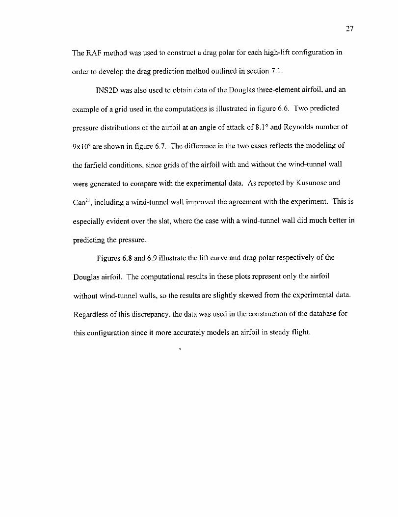
TheRAF methodwasusedto constructadragpolar for eachhigh-lift configurationin
orderto developthedragpredictionmethodoutlinedin section7.1.
INS2Dwasalsousedto obtaindataof theDouglasthree-elementairfoil, andan
exampleof agrid usedin thecomputationsis illustratedin figure6.6. Two predicted
pressuredistributionsof theairfoil atanangleof attackof 8.1° and Reynolds number of
9x 10⁶ are shown in figure 6.7. The difference in the two cases reflects the modeling of
the farfield conditions, since grids of the airfoil with and without the wind-tunnel wall
were generated to compare with the experimental data. As reported by Kusunose and
Cao 2_, including a wind-tunnel wall improved the agreement with the experiment. This is
especially evident over the slat, where the case with a wind-tunnel wall did much better in
predicting the pressure.
Figures 6.8 and 6.9 illustrate the lift curve and drag polar respectively of the
Douglas airfoil. The computational results in these plots represent only the airfoil
without wind-tunnel walls, so the results are slightly skewed from the experimental data.
Regardless of this discrepancy, the data was used in the construction of the database for
this configuration since it more accurately models an airfoil in steady flight.

28
Douglas LB-546
NLR-7301
Figure 6.1 Two and Three-Element Airfoil Geometries
_ l-l--l-_l
Figure 6.2 Sample CHIMERA Grid of the NLR-7301 Two-Element Airfoil

29
-8
-7 -- INS2D i• Experimental
-6
-5
-4
Cp -3
-2
-1
0
1
2
0 2 0.4 0.6 "_t_.._ll 1.2
t q i i b t _ I I ', I I _, .... , , , , I
x/c
Figure 6.3 NLR-7301 Pressure Distribution (a=6 °, Re=2.5 lxl0 6)
1.4
I
C 1
3.5 _ l INS2D /
3! / ° Experimental__
2.5 y -2 • •
1.51 I
I
o.soT
0.0
b , I F I i p n I t _ t I I i I
5.0 10.0 15.0(deg)
Figure 6.4 NLR-7301 Lift Curve (Re=2.5 lxl06)

30
C d
0.045
0.040
0.035
0.030
0.025
0.020
0.015
0.010
0.005
0.000
• Experimental
• INS2D__ RAF Method
0 0.5 1 1.5 2 2.5 3 3.5Ci
Figure 6.5 NLR-7301 Drag Polar (Re=2.51 x 10 6)
Figure 6.6 Sample CHIMERA Grid of the Douglas LB-546 Three-Element Airfoil

31
I INS2D - Freestream..... INS2D Wind-Tunnel Wall
I ExperimentalI •
x/c
Figure 6.7 Douglas 3-Element Pressure Distribution (c_=8.1 o, Re=9.0x 10 6)
C I
2
0
INS2D |] • Experimental| j__
0
I q t I I I t i i I I t I I j I I I _ J i _ I _ I I I I I I I I I I I
5 10 15 20 25 30 35(deg)
Figure 6.8 Douglas 3-Element Lift Curve (Re=9.0x 10⁶)

32
C d
0.14
4-
0.12 _7_
0.1
t • Experimental n
• INS2D I__ RAF Method
0.08
0.02
J
y
0T _ _ i I I i b i i I _ _ I t t I i I t I ! I i I i
0 1 2 3 4 5Ci
Figure 6.9 Douglas 3-Element Drag Polar (Re=9.0xl0 6)

7.0 Aerodynamic Module
33
Thenewly developedhigh-lift modulepredictstheaerodynamicperformancefor
agivenhigh-lift systemto beusedwithin atakeoffandlandingoptimization routine such
as ACSYNT. It calculates lift, drag, pitching moment, and maximum lift for a given
high-lift system and flight conditions.
The high-lift module first calculates two-dimensional aerodynamic characteristics
from equations based on CFD and wind-tunnel data. These aerodynamic characteristics
consist of sectional lift curve, profile drag polar, and pitching moment which are
calculated from basic airfoil geometry. A modified lifting-line method based on
Weissinger's theory 22is then used to determine the total aerodynamic coefficients of the
wing. Thus total lift, drag, and pitching moment can be computed faster than with a
panel method while incorporating (based on strip theory calculations) the viscous effects
of slotted high-lift devices.
7.1 Two-Dimensional Aerodynamics
Theoretical and empirical techniques were applied to develop equations based on
the high-lift configuration type, c, t/c, %E_rE, 8EEriE, Ct, C_oc_e, C_, sl, and s2 from the two-
dimensional database in order to calculate s o, C_, Cdpronle, and Cmo.

7.1.1 Lift
34
A flap is used to produce added lift by increasing the effective camber of an
airfoil. Thus, the total lift of an airfoil with extended high-lift devices is represented by
the lift of the clean airfoil plus the incremental lift created by the leading and trailing-
edge flaps:
C I
= -- + ACIT E + ACIL E (7)el C Iclean C
The lift coefficient for the clean airfoil at a given angle of attack is provided by
ACSYNT. The increment in lift coefficient is a function of the flap configuration,
geometry, and deflection angle. The additional lift produced by a single-slotted trailing-
edge flap is shown below as defined in DATCOM: 2_
C r
-- (8)ACITE ----Claclcan (X'5_TE c
The lift-effectiveness, c%, is determined for a specified flap configuration type with the
general equations shown below:
(/',5 -- -- C + Z (/'.6theory ft/cfvisc + (9)
=--ZI_/CTE (1--CTE/ + sin-t _/-_1 (10)¢X'sthe°ry x L_/ c ,. c J
Z = [1 + al • tan-I(a2 .STEXl )] fcf (11)
fcf = 1 - b_ • cTE (12)C

35
ft/c = 1 + c I • t/c (13)
fvisc =dl (14)
where a_, a 2, b,, c_, dj, and x_ are empirical coefficients and were determined to be as
follows for both the NLR and Douglas flaps:
a_ = 0.2, a2 = -5.2, b, = 0.55, c, = 1.04, d_ = 0.785, xl = 5
The expression for the theoretical lift-effectiveness, o%,heo_y,is derived for a bent
flat plate in an inviscid flow and is a good approximation for small flap deflections. 24 It is
a function of the flap chord, c_, only, but an empirical airfoil thickness factor, f_c, and
viscous factor, fv,sc, have been added to account for Reynolds number by scaling c%,heo_y
with CFD or experimental data. The separation factor, Z, is used to reduce the lift-
effectiveness, as, at higher flap deflection angles. The empirical factor is roughly unity at
small flap deflections but decreases at larger deflections to account for strong viscous
effects and flow separation over the flap. This factor is dependent on the configuration
type and the Reynolds number of the CFD or experimental data. Examples of the
separation factor and lift-effectiveness curves for the NLR-73 01 airfoil are illustrated in
figures 7.1 and 7.2 respectively.
It should be noted here thai the lift increments of the NLR flap and Douglas flap
calculated with this method are both higher than the lift increment of a double-slotted flap
calculated via DATCOM. 23 This illustrates the importance of the present methodology,
since it is obvious that the performance of current high-lift systems can no longer be
predicted with methods that are based on outdated technology and low Reynolds number
data.

36
Theprimarytaskof aslator KrUgerflap is to extendthelift curveby increasing
thestall angleandasaresultincreaseawing'smaximumlift capability. However,a
leading-edgedevicewill slightly alterthe lift of awing. This lift incrementis often
negligibleandmaybedisregardedin thepreliminarydesignphase,but if theeffect is
desired,lineartheorymaybeusedfor a goodfirst approximation.Theadditionallift
producedby a leading-edgedeviceis calculatedfrom:
C I
-- (15)AGILE = Clotclean (_Sthe°ry_LE C
where Roshko 25shows that the theoretical lift-effectiveness of a leading-edge device is:
2 II-_( CTE/ -sin-I _et_the°rY -- rt 1-- C J (16)
The extended chord length, c', is calculated from geometric properties of the
leading and trailing-edge devices. This increase in chord is produced by so-called Fowler
action and is a very important characteristic of a high-lift device. It can dramatically
improve the lift performance of an aircraft without producing excess drag. Examples of
Fowler action are shown below for an airfoil with a leading-edge device and a single or
double slotted flap.,D
Single slotted flap:
c' =c+f.s 1 +d'CLE (17)
The Fowler action functions, f, of the flap and, d, of the slat can be specified by the user,
or the default functions may be used. The flap function is based on the assumption that
full Fowler motion is reached at a deflection angle of 45 ° and is specified as:
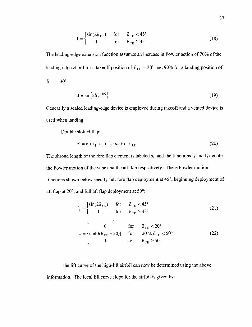
37
sin(2?TE) for 8TE< 45°f = for 6TE> 45 °(18)
The leading-edge extension function assumes an increase in Fowler action of 70% of the
leading-edge chord for a takeoff position of 8 LE ---- 20° and 90% for a landing position of
SEE = 30 °.
d = sin(2_SLE °9) (19)
Generally a sealed leading-edge device is employed during takeoff and a vented device is
used when landing.
Double slotted flap:
c' = c + fl "sl + f2 ' s2 + d. c LE (20)
The shroud length of the fore flap element is labeled s2, and the functions t"1and t"2denote
the Fowler motion of the vane and the aft flap respectively. These Fowler motion
functions shown below specify full fore flap deployment at 45 ° , beginning deployment of
aft flap at 20 ° , and full aft flap deployment at 50°:
{sin(2? TE) f°r 5TE<45° (21)fl = for 5TE _>45 °
(22)f 0 for _TE < 20°
f2 = sin[3(5 E -- 20)] for 20°< 5TE < 50 °
for _TE _ 500
The lift curve of the high-lift airfoil can now be determined using the above
information. The local lift curve slope for the airfoil is given by:

38
C t
-- (23)Cla = _Claclean c
Note that the separation factor Z appears once again; this time it accounts for a deviation
in the lift curve slope from 27t rad -1. Finally, the angle of attack at zero lift for a flapped
airfoil can be calculated from:
(24)
where the local lift coefficient at zero angle of attack is determined as shown below:
C t
= -- + ACvr E + ACIL E (25)Cl° Cl°clean c
7.1.2 Drag
A database of minimum drag coefficient, Cdmin , lift coefficient at minimum drag,
Ctm_, and profile drag constant, 1%,was constructed using the RAF parabolic polar
estimation method. Once this database was established, equations for the increments in
Cdm_, C_,,_, and 1%were determined by fitting curves to the data. The following equations
represent the increments associatfd with a single-slotted trailing-edge flap:
c__ACdminTE =al_TEXl\ 0.3) C
(26)
AClminTE = (biB"rE - b28TEX3 CTE --C (27)
AkpT E (ciS.rE +c 8 2](CTE']x5 C= 2 TE )C-'O_") _"
(28)

39
wheretheempiricalconstantsandexponentsgivenbelowarefor boththeNLR and
Douglasflaps:
a_=0.038,b_=2.3,bz=2,ct=0.00012,c2=0.0097,
x_=1.74,x2=1.4,x3=4,x4=-0.17,x5=2.55
Theincrementaldragcoefficientfor a leading-edgeflap is extremelydependent
on theconfigurationtype,deflectionangle,andgapsetting. Therefore,nogeneral
empiricalmethodfor calculatingdragincrementhasbeendeveloped.InsteadCFDdata
isusedexplicitly to give dragincrementbasedon theconfigurationtested.The Douglas
slat is used here to give drag polar information for both the takeoff and landing settings:
Takeoff (_LE=20°):
C ?
ACdminLE = 0.0013--c (29)
C !
ACIminLE = 0.46--c (30)
C
Akp LE -- 0.00772 _ (31)
Landing (6eE=30°):
,, C t
ACdminLE = 0.0074--c (32)
C ¢
ACiminLE = 0.76--c (33)
c= 0.00381-- (34)
AkpLE C'
The drag polar components of the high-lift airtbil are calculated from the
contributions of both the leading and trailing-edge devices and the clean airfoil:

C t
--+ +Cdmin = Cdminclean C mCdminTE ACdminLE
(35)
e I
--+ +Clmin = Clminclean c ACIminTE ACIminLE
(36)
C+ + Ak (37)
kp = kpclean --c' AkpTE PLE
These coefficients are then used to construct the following airfoil drag polar which is
used to determine profile drag at each section:
Cdprofil e = Cdmin -t- kp(C t - Clmin )2 (38)
40
7.1.3 Pitching Moment
The pitching moment about the aerodynamic center (or at zero lift) of the high-lift
airfoil is calculated from the pitching moment of the clean airfoil and the contributions
from the leading and trailing-edge devices:
Cmo = Cmoclean + ACmoT E mOLE
The increment in the pitching moment coefficient at the aerodynamic center due
to the trailing-edge device is:
moT E = ACIT E
The position of the center of pressure, --
xeP c"lc' (40)
Xcp
c; ' for an airfoil with a single-slotted flap is
determined empirically as:

41
Xcp- 0.5 -- alSTEXl (41)
C'
The empirical coefficients a_ and xt were determined to be as follows for both the NLR
and Douglas flaps:
al = 0.134, Xl = 0.46
The pitching moment increment at the aerodynamic center due to the leading-edge
device is:
t_ 2
AC mo LE = C m3LE _ LE _,7)(42)
and 0LE is specified as:
OLE =c°s-l( 1-2cLz/c J (44)
The sectional pitching moment about an arbitrary reference point xre----Lfisc
measured from the leading-edge of the clean airfoil is determined as:
Cmxref = Cmo +(C I cosct +C d sintx)( Xref Xac) (45)C C
where Cd includes both the profile drag and induced drag at the section.
(43)C m6LE = - I sin 0 LE (1 -- COS0 LE)
where the pitching moment effectiveness about the aerodynamic center is found from thin
airfoil theory: 26

42
The aerodynamic center of the high-lift airfoil is only a function of Fowler action,
and its position relative to the leading-edge of the clean airfoil is found by determining
the individual shifts in --X ac
Cdue to the leading and trailing-edge devices:
Xa-c _ -- - (46)
c c clean c LE
where is the extended chord resulting from only the Fowler action of the leading-LE
edge device.
7.2 Three-Dimensional Aerodynamics
A modified lifting-line method based on Weissinger's theory is applied to
determine the spanwise loading across the wing. From this procedure a load distribution
can be calculated for a wing of arbitrary planform from sectional lift curve slopes and
angles of zero lift. Thus, the total aerodynamic coefficients of the wing can be calculated
from a combination of two- and three-dimensional methods. This results in a prediction
method which is relatively fast ana reflects the viscous nature of slotted flaps.
The Weissinger method accounts for partial span flaps/slats, aspect ratio, and
Mach number in order to calculate lift, downwash angle, induced drag, and pitching
moment. The geometry of the wing may be asymmetric about the centerline and can
include sweep, taper, and twist. The method models the wing as a plate of zero thickness,
but the planform and twist remain identical to the actual wing. Thus, partial span flaps

43
and Fowler action may be modeled as discontinuities in twist and an increase in chord
length respectively.
The chordwise load distribution at each span station is concentrated into a lifting
line located at the wing's quarter-chord line. The theory requires that the quarter chord
line is straight, yet a discontinuity is allowed at the plane of symmetry so that a swept
wing may be considered.
The method assumes that the lifting line and its trailing vortex sheet are
continuous. However, discrete values for the circulation strength are determined only at
the span stations along the quarter-chord line corresponding with control points. The
number of control points is specified, and each point is placed at the three-quarter-chord
line. Mathematically this implies that the lift curve slope is 2rt rad _, so a correction
method must be incorporated for a lift curve slope that varies from the theoretical value.
For further details please refer to the outline of this correction method in Appendix A.
The general input parameters required by the method are a, AR, rleErrE, A, _,, M,
and S, and the following parameters must be specified at each control point: et o, C_, c, _w.
The chord is defined to be parallel to the freestream direction in the Weissinger method
as shown in figure 7.3, so caution'should be taken to ensure that all aerodynamic data
represent streamwise values. Simple sweep theory dictates that two-dimensional data
should be modified from normal (n) to streamwise values as follows:
z/c = (z/c)n .cosA (47)
M = M,/cosA (48)

Re= Ren/cos2A (49)
= (C,,_)n.cosA (50)
C m =(era) n .cosA (51)
Also, recall that % and C_ were determined previously from sectional CFD and
experimental data and are based on the appropriate Reynolds number.
44
7.2.1 Lift
The Weissinger method determines the local lift coefficient, C_, at each control
point along the wing. From this load distribution the total lift coefficient of the wing, CL,
is determined. The method also returns values for the total lift coefficient of a wing at
zero angle of attack, CLo, the lift curve slope of wing, CL, and the downwash angle
distribution, _.
Two test cases were used to validate the results of the Weissinger method. Figure
7.4 shows one of these test cases. It is a part-span-flap wing/body configuration with
variable twist, and figures 7.5 and'7.6 compare the experimental data 27of this model with
predicted load distributions. The other test case is a plain swept wing and is shown in
figure 7.7. Similarly, figures 7.8 and 7.9 compare the experimental data '8 of this
configuration with calculated lift distributions. Both validations compare relatively well
with the experimental data; however, there is a slight disagreement at the root of the
wing. This discrepancy exists because a body was not modeled computationally in either
test case, while both of the experimental models were wing/body configurations.

45
7.2.2 Dra_
Total drag is calculated from both profile drag and induced drag contributions.
The Weissinger method determines only the induced drag coefficient, C W so further
calculations are required to determine the total drag coefficient of the wing.
Two-dimensional drag polar data is used to calculate the total profile drag by
integrating local profile drag across the wing:
)2Cdorotile = Cd min + kp (C I - Clmin at station rl
(52)
Ybody b/21 1
CDpr°file - S j'cdcdy + S j'Cdcdy
- b/2 Ybody
(53)
where Ybody represents the y-coordinate of the exposed wing root. For a symmetric wing,
this reduces to:
2 b/2
CDor°nle - S _[Cdmin + kp (C I - Ctmin )2 ]cdy (54)
Ybody
The total drag coefficient can now be found by summing the profile drag and induced
drag coefficients:
CD = CDprofile + CDinduce d (55)

7.2.3 Pitching Moment
46
The total pitching moment about a reference line which is normal to the
freestream velocity is calculated as:
b/22
jC mxre f cdyCMxref -- S
Ybody
(56)
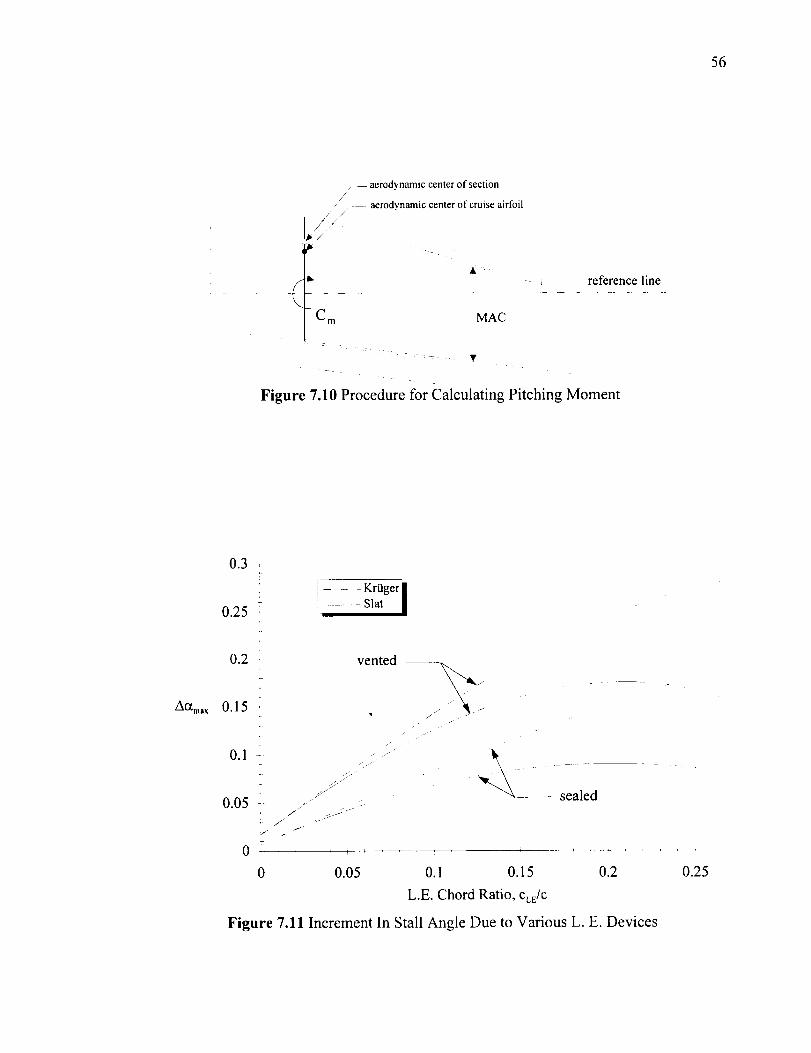
where the local pitching moment is calculated as shown earlier:
Cmxref =Cmo+(Clcoso_+Cdsino_)(Xc f x_e) (57)
X re fHere, the position --
Ccorresponds to a point on the reference line as shown in figure
7.10.
7.3 Maximum Lift Prediction
Maximum lift and stall angle are also calculated using both two- and three-
dimensional methods. The maximum local lift coefficient at each spanwise station along
the wing is calculated from empirical equations generated from the two-dimensional
database. Weissinger's theory is then used to determine the onset of stall by finding the
critical section. This method is used to predict maximum lift in the preliminary design
process, but other more sophisticated methods should be used in subsequent design
phases.

47
Onesuggestedmethodthatcanbeimplementedinto thepresentmethodologyis
thepressuredifferencerule developedby ValerezoandChin.29 This method predicts the
maximum lift of an airfoil based on the difference in the peak pressure coefficient and the
pressure coefficient at the trailing-edge of an airfoil. The pressure difference rule
compares chordwise pressure distributions scaled by their corresponding peak pressure
coefficients with a prescribed pressure difference at maximum lift to determine the onset
of wing stall for a specified Mach and Reynolds number. This correlation has shown
remarkable results and has demonstrated that the method works well for both clean and
multi-element airfoils alike, assuming the leading element stalls first.
7.3.1 Two-Dimensional
Empirical equations based on CFD and wind-tunnel data are used to calculate
maximum lift at each specified wing station. The general input parameters used to
calculate maximum lift are: high-lift configuration type, c, t/c, %zqx, s_, s2, 6eznx, rlez_,
A, M, and Re.
The maximum local lift colefficient is calculated from the maximum lift of the
clean airfoil and the maximum lift contributions from the leading and trailing-edge
devices:
C t
--+ +Clmax = Clmaxclean c mCImaxLE mCImaxTE
(58)
Clmaxclean clean maximum lift coefficient

AClmaxLE
mClmaxT E
48
- lift coefficient increment due to the leading-edge device
- lift coefficient increment due to the trailing-edge device
The increment in maximum lift from a leading-edge device results from a shift in the stall
angle of the airfoil:
AClmaxLE = Cla A_ma x (59)
A_ma x =a I +a2/cLE. +a 3 +a 4 (60)\ C / \ C J
The shift in stall angle is only a function of configuration type and leading-edge chord
length since the maximum lift performance is fairly insensitive to the angle of the
leading-edge device if the gap and overhang are properly optimized:" 30 As mentioned
earlier, this shift in angle is constant regardless if the trailing-edge flaps are stowed or
deployed. Figure 7.11 illustrates AOtmax, and table 7.1 gives values for the empirical
constants a,, a2, a3, and a4.
The increase in maximum lift created by trailing-edge flaps is determined using a
type of maximum lift-effectiveness parameter, C,sm_x:
C'
ACImaxTE = CI3max6TE C
,I
Climax =(al +a28TEXl)fcf
(61)
(62)
fcf = (CTE/X2 (63)k 0.3)
where the empirical constants used to calculate the increment in maximum lift for single-
slotted flaps are:

at=153.4,a2=-151.8,x_=0.018,x2=0.16
49
7.3.2 Three-Dimensional
Weissinger's theory is applied to determine the lift distribution across the wing,
and the maximum lift is predicted using a critical section approach. It is assumed that the
onset of stall occurs when one wing section reaches its maximum lift as illustrated in
figure 7.12, yet the wing continues to lift past this critical angle of attack as reported by
Murillo and McMasters. 3_ The maximum lift of the wing is evaluated as:
CLmax = CL(C%rit ) + f(Re) (64)
where Ce(c_cn,) corresponds to the lift coefficient at the critical angle of attack, and the
function f(Re) is Reynolds number dependent and is assumed to be 10% of Ce(ctc,,) at the
present.
The polynomial method for optimization 32is used to find the critical angle of
attack since sectional lift curves may be non-linear. The difference between the local lift
coefficient and the local maximum lift coefficient is found at each spanwise station from
( ) isdete ined,the provided load distribution. The minimum difference, C s - Ctm _ mi.'
and the objective function is defined as:
f(_) = (CI - Cim_tx)min (65)
The polynomial optimization method is then used to minimize this function in order to
determine the critical angle of attack.

50
Sea,edSlotIVentedSlatISeale__gerIVented_geral 0.0068 0.017 0.0068 0.017
a 2 0.81 1.28 0.81 1.28
a 3 -1.88 -1.35 -0.37 0.32
a4 -0.38 -5.5 -0.357 -5.3
Table 7.2 Variables Used to Calculate the Maximum Lift-Effectiveness
of Leading-Edge Devices

51
1
0.9
0.8
0.7
0.6
Z 0.5
0.4
0.3
0.2
0.1
÷
0
0
• z•
CrE/C
--0.1
..... 0.2
0.3
-- 0.4
10 20 30 40 50
Flap Deflection (deg)
Figure 7.1 NLR-7301 Separation Factor
6O
0.7
0.6
0.5
0.4
0.1
i ....
crJc0.1
-0.2
0.3
0.4
t
+
T
0
, I
10 20 30 40
Flap Deflection (deg)
Figure 7.2 NLR-7301 Lift-Effectiveness
50 6O

52
q_
[,J oo
1
r
2-D
Reynolds Averaged N-S Method
3-D
Modified Lifting-Line Method
Uoo
Section A-A T)
,a;
Figure 7.3 Overview of Aerodynamic Analysis

53
Wind-tunnel measurements using a variable twist wing (VTW) model in the NASA
Langley 14- by 22-Foot Tunnel at a Reynolds number of lxl06 and lift coefficient of 0.6.Y
Dots indicate 20 semispan locations/_ I X
2er:.%.2: 2? '72...M. i
( 11 I1 /
_. 3556 -,H Body-of-revol utl on
m wing-tip cap 7
{ [fill[ IlfllilI III Ill [ Illll Ill tim IIIJ _ _llllll[lllill II]lll Ill Illl 1) Ill)I I1}
_L _-_,-,2,od,,°Width of each segment,
2.96 cm
Wing Characteristics
Area, S ..........
Semlspan, s ......
Chord, c .........
Aspect ratio .....
Taper ratio ......
Airfoil section --
Segment width ....
0.B852 m 2
1.245 m
0.3556 m
7
I
HACA 00,2
0.02964 m
.3556 Z_
/ --19.76 °
,0,0 L_000,-L.,otI- , .067 4
*Cy, indrical body length
Figure 7.4 Part-Span-Flap Deflection Test Case (from Ref. 27)
Ci
0.8
0.6
0.4
0.2
0
0
Experiment-- Weissinger Method
_ Vortex-Lattice Method (NARUVL) I !I i I
. I I I
-_ q I
I I
__ _ ___ _
I
"-,.,,. I
I ,s I
I I
I
I
....... I ...............
I
Body radius
I I
I I
I I
I
I I q 1 I I i i I
0.2 0.4
I
I
I
I
I
I
I
q I i
0.6
y/(b/2)
I
I
I
I
Act, deg
__ 10-15
I
I i I _ I I -20
0.8
Figure 7.5 Part-Span-Flap Spanwise Load Distribution
VTW7S 1 Configuration, ct= 11.4 °

54
el
Experiment-- Weissinger Method
_ Vortex-Lattice Method (NARUVL) [ /
0.8
0.6
0.4
0.2
T I k I-4-
I q F I
I d I I
i .......
I
0
0 0.2 0.4 0.6 0.8
y/(b/2)
Figure 7.6 Part-Span-Flap Spanwise Load Distribution
VTW7 Coi_figuration, a=8.5 °
-5
Act, deg
-10
-15
-2O
Wind-tunnel measurements using two semispan wing-fuselage models in the NASA
Ames 40- by 80-Foot Tunnel at a Reynolds number of 8x10⁶.
NAGA 64A-010 (plain wing)NAOA 64A-810 [cambered,twistedwing)
Pitching-momentaxis (0.25 E)
chord
Note,AlLdimensionsgiven infeetunlessotherwisespecified
12.00R
24.42
Figure 7.7 Swept-Wing Test Case (from Ref. 28)

55
0.5• Experiment iWeissinger method
Cl
0.4
0.3
0.2
0.1
0
I I I
0.2 0.4 0.6
y/(b/2)
Figure 7.8 Swept-Wing Lift Distribution
Plain Wing Model, CL=0.4
I i I I b
0.8
0.5
• Experiment i-- Weissinger method
0.4
0.3
CI
0.2
0.1
0 0.2 0.4 0.6
y/(b/2)
Figure 7.9 Swept-Wing Lift Distribution
Cambered & Twisted Wing Model, CL=0.4
0.8
56
/ aerodynamic center of section/
/ aerodynamic center of cruise airfoil
// ///
/ /
_/ .....
(_ - ; reference line
C m MAC
Figure 7.10 Procedure for Calculating Pitching Moment
Z_m_x
0.3
0.25
0.2
0.15 -
o.li
0.05 -
-f
01-
0
- KrUger I
Slat |
vented
J .f/_/¸/
1
sealed
0.05 0.1 0.15 0.2
L.E. Chord Ratio, CLE/C
Figure 7.11 Increment In Stall Angle Due to Various L. E. Devices
0.25

57
Clrnax
Cl
C_ at stall _ ._ _
critical section ----------_ _._ -.C,((y_crit) " " -"_
CLm_ = CL(CZcnt) + fiRe)
I i I
Spanwise Station, rl
Figure 7.12 Maximum Lift Estimation Using Critical Section Approach

8.0 Weight Module
58
The weight of the high-lift system is an important factor in the preliminary design
phase of an aircraft. The system weight is very much govemed by the aerodynamic
loads, the structural materials, and the structural stiffness requirements. Other important
factors that may affect the overall weight of the high-lift system are fail-safe design
requirements, system complexity, and system reliability. However, it is important to note
that information on the weight and the aerodynamic performance of a high-lift device is
not sufficient to determine the optimal system. The optimal system depends on the
effects of the high-lift system on the weight and cost of the complete aircraft. For
instance, a variable camber Krfiger flap may be heavier than a slat; yet, as a result of a
slightly higher maximum lift, it may produce a substantial increase in maximum payload
for a given aircraft geometry and mission profile.
This estimation method was developed to offer a parametric weight sensitivity
analysis for weight and cost trade-off studies. It uses empirical equations based on
historic data to calculate incremental weights due to leading and trailing-edge devices.
The method predicts leading and trailing-edge surface, support, support fairing, actuation,
and fixed structure weights for a given high-lift system. As a result, changes in the
technology of materials, geometry, mechanisms, or actuation can be reflected through the
scaling of the various weight components.
The equations are based solely on stowed flap area, so they require minimal
geometric data to evaluate system weight in the preliminary design phase. This

representsa reductionin complexityfrom existingweightestimationmethodssuchas
thoseby Andersonet al.33andOman.34Thesemethods,whicharebasedonnumerous
high-lift parameters,areverydifficult to correlatewith the limited datathat is available,
andtheyoftenresultin trendsthatarenotrealistic. Thus,asimplerapproachwas
adoptedto constructafast,robust,andfairly accurateweightpredictionmethodfor
multi-elementwings.
59
8.1 Trailing-Edge Flap Weight
Flap panel, support structure, support fairing, and actuation weight correlations
are shown below. These weights are based on stowed flap area for a given flap
configuration and support type. The specific weights a_, a2, a3, and a4 are given in tables
8.1 - 8.3. Trailing-edge weight correlations are shown for several aircraft in figure 8.1.
Surface Structure:
Wpanel = al "aTE
Support Structure:
W_.ppo_t = a2- flow" S-rE
{41 Rf°_
0. 7+0.53--
frow = 0.5
for linkage and external hinge supports
for track supports
(66)
(67)
(68)

Rfow- ASv°wle_r (69)STE
where ffowis a function of Fowler motion and is used to scale the weights of linkage and
externally hinged supports and fairings. The term Rfow is the ratio of Fowler area to the
area of the trailing-edge flap.
60
Support Fairing:
Wfairing = a3 "ffow "STE (70)
Actuation:
Wactuatio n = a 4 • STE (71)
Total Trailing-Edge Flap Weight:
WTE = Wpane I + Wsupport + Wfairing + Wactuatio n (72)
The fixed trailing-edge weight of the wing is also determined in order to calculate
the total wing weight. This weigl_t is estimated using the equation developed by
Anderson et al.: 35
WnxeaTE 1.34(S nxed.r E )1.089= > 2.0. S n×_dVE
where SnxedvEis the area of the fixed trailing-edge and is calculated as:
SfixedTE = STEgross --(STE + Sai I -I- 0.5" Ssp )
(73)
(74)

Thegrosstrailing-edgeareaof thewing is representedby SVEross,andtheaileronand
spoilerareasaredenotedasS,_andSsp,respectively.
61
8.2 Leading-Edge Flap Weight
As with the trailing-edge flaps, the leading-edge device component weights are
based on nested flap area as shown below. The specific weights as, f16,and a7 are given in
table 8.4, and correlations for leading-edge weights of several airplanes are plotted in
figure 8.2.
Moving Panels:
Wmoving = a 5 "SLE (75)
Actuation:
Wactuation = a 6 "S LE (76)
Fixed Leading-Edge:
Waxed = a 7 "S LE (77)
Total Leading-Edge Flap Weight:
WLE = Wmoving + Wactuatio n + Waxed (78)

62
Theabovemethodsfor predictingleading-edgedevice,trailing-edgedevice,and
fixed trailing-edgeweightalongwith themethodsfor estimatingaileronandspoiler
weight(shownin AppendixB) will beusedin conjunctionwith thewing boxweight
estimationmethoddevelopedby Ardemaet al. 36 to determine the total weight of the wing
within ACSYNT.
This prediction method is intended to be used only in the preliminary design
phase of an aircraft. However, the methodology lends itself to an improved weight
estimation method for subsequent design phases, since experimental data shows 3vthat
flap loading is independent of angle of attack and is only a function of flap deflection.
The proposed idea involves changing the routine from a 0 'h order to a 1s' order predictive
method so that CFD results can be used in conjunction with slender beam analysis to
determine the weight of a configuration. Thus, the chordwise load distribution supplied
by CFD and the spanwise load distribution provided by the Weissinger method can be
used to determine the weight of a high-lift system for a given flap placard speed
(maximum speed allowed with flaps deployed) with a specified support type and number
of supports.
Once this method is devel6ped, the loading information provided by CFD can also
be used as an input in the calculation of wing box weight. This will provide valuable
information for calculating the torsional loads produced by the flaps. Consequently, the
structural analysis of the wing box will include information regarding the flap
configuration and Fowler action.

63
SpecificWeight
Single-Slotted FixedVane/Main
ArticulatingVane/Main
3.5
Main/Aft
4.8
Triple-Slotted
5.5FlapPanel (a_) 2.7
Support (a2) 3.0 3.2 3.8 4.7 5.6
Fairing (a3) 1.0 1.0 1.15 1.3 1.4
Actuation (a4) 2.2 2.2 2.3 2.4 2.5
Total 8.9 9.4 10.75 13.2 15
Table 8.1 Specific Weights of Trailing-Edge Flaps with Hooked Track Supports
(lb / ft 2 of stowed flap area)
Specific
Weight
Single-Slotted Fixed
Vane/Main
Articulating
Vane/Main
3.5Flap Panel (a_) 2.7 3.0
Support (a2) 1.5 1.6 1.9
Fairing (a3) 0.11 0.11 0.13
Actuation (a4) 2.0 2.0 2.1
Total 6.31 6.71 7.63
Main/Aft Triple-Slotted
4.8 5.5
2.4 2.8
0.14 0.16
2.2 2.3
9.54 10.76
Table 8.2 Specific Weights of Trailing-Edge Flaps with Link/Track Supports
(lb / ft 2 of stowed flap area)
Specific
Weight
Single-Slotted
Fairing (a3)
Fixed
Vane/Main
ArticulatingVane/Main
Main/Aft
Flap Panel (a 0 2.7 3.0 3.5 4.8
Support (a2) 1.1 1.2 1.8 2.2
0.28 0.28 0.29 0.29
Actuation (a4) 0.9 1.0 1.3 1.5
Total 4.98 5.48 6.89 8.79
Table 8.3 Specific Weights of Trailing-Edge Flaps with External Hinge Supports
(lb / fi2 of stowed flap area)

64
FlapType FixedCamberKrtiger
VariableCamberKrtiger
MovableL. E. (as) 4
Actuation(a6) 2.8
6
Slat without
Slave Tracks
Slat with
Slave Tracks
5.1 7.7 8.5
2.8 2.1 2.1
8.5 4.5 4.7Fixed L. E. (aT)
Total 12.8 16.4 14.3 15.3
Table 8.4 Specific Weights of Leading-Edge Devices
(lb / ft 2 of stowed flap area)

65
¢3._
//
• 72_1 f757/
.7.3 7•oc-8
• MD-83
/
z
• MD-II
•rz
/•
J/
///z
,/
/ z
• 747
Actual Weight
Figure 8.1 Trailing-Edge Weight Correlations for Various Aircraft
3:
• 727 ......
/"/
/
/-
•/r
/'
/
///
/./
/
,/
//`•/
J
J
• MD-83
/
/
z_0 74_ MD-II
Actual Weight
Figure 8.2 Leading-Edge Weight Correlations for Various Aircraft

9.0 Cost Module
66
The impact that a high-lift system has on the total life cycle cost of a transport
aircraft is a complex function of the costs to develop, build, purchase, operate, maintain
and dispose of the airplane. As described by Gelhausen 38, the total cost of the system is
best captured in the direct operating cost (DOC) where the costs to own and operate the
aircraft are combined. The DOC includes fuel, airframe, crew, and maintenance expenses
and is the most important parameter used when comparing civil transport aircraft with
equivalent missions. A full mission and market analysis is required to show the effects of
improved high-lift system performance. This includes improved fuel economy, the
increase in range and payload, and the increase in units sold. However, the cost to
manufacture and maintain the system must be analyzed in order to understand the
complete picture. For instance, a system that is more complex but generates a higher
maximum lift may result in improved cruise efficiency and reduced fuel expenditures, but
at the same time may cause increased airframe and maintenance cost. It is important to
not only provide the aerodynamic and weight information, but also the cost information
to the synthesis process. This methodology incorporates system cost so that careful
tradeoff studies can be conducted to determine the optimal high-lift system for a new
aircraft.
The system cost is governed by the weight, W, and the part count, PC of the high-
lift device: 39
Cost = a I •W.PC xl (79)

67
1.8881 trailing - edgedeviceal = [1.7339 leading- edgedevice
xl=0.7
Heretheconstant,al accountsfor hourly laborcostsandtypeof material. Historically,
weighthasbeenthemostimportantparameter,but recentlymoreinformationregarding
partcounthasalsobecomeavailable.For instance,Boeingsimplifiedtheflap systemon
thenew737from a triple-slottedto adouble-slotteddesign.Thenew flapsystemhas
37%fewerpartsand33%fewerbearings.4°Thisreductionin partaffectscost(note,
however,thatthereductionin costis reportedto besignificantly lessthan30%indicating
avaluefor thepartcountexponent,x_,significantlylessthanunity) and,consequently,
thenewlydevelopedcostmoduleincorporatesthis factoraswell assystemweight.
Thetotalpartcountof asystemis foundby summingup thevariouscomponents
of thedevice. Thepartcountof atrailing-edgeflapconsistsof theflappanel,support,
supportfairing, andactuation:
PCTE = PCpane I + PCsuppo_t + PCfairing + PCactuatio n (80)
The part count of a leading-edge device is the sum of the movable leading-edge,
actuation, and fixed leading-edge:,
PC LE = PC movable + PC actuation + PC fixed (81 )
Each category is a function of the flap configuration and support type only. The total part
count is used as a measure of overall system "complexity", while the size of the device
and complexity associated with Fowler action are reflected in the weight of the flap.
Values for part count components of trailing-edge devices are given in tables 9.1 - 9.3,
and component values for leading-edge devices are given in table 9.4.

68
PartCount Single-Slotted Fixed ArticulatingComponent Vane/Main Vane/Main
FlapPanel 820
Main/Aft
1400
Triple-Slotted
1620600 750
Support 210 210 230 230 260
Fairing 350 360 370 380 500
Actuation 450 450 450 450 450
Total 1610 1770 1870 2460 2830
Table 9.1 Part Count of Trailing-Edge Flaps with Hooked Track Supports
Part Count
Component
Flap Panel
Single-Slotted
600
Support 150
Fairing 100
Actuation 300
Total 1150
Table 9.2
Fixed
Vane/Main
Articulating Main/Aft
Vane/Main
820 1400
Triple-Slotted
1620750
150 164 164 185
100 105 110 145
300 300 300 300
1300 1389 1974 2250
Part Count of Trailing-Edge Flaps with Link/Track Supports
Part Count
Component
Flap Panel
Single-Slotted Fixed Articulating
Vane/Main Vane/Main
810
Main/Aft
1380590 740
Support 200 200 220 220
Fairing 200 205 210 220
Actuation 200 200 200 200
Total 1190 1345 1440 2020
Table 9.3 Part Count of Trailing-Edge Flaps with External Hinge Supports

69
PartCountComponent
MovableL. E.
SlatwithSlaveTracks
FixedCamberKrfiger
SlatwithoutSlaveTracks
800
VariableCamberKrUger
1000 840
Actumion 300 300 300 400
]FixedL.E. 1400 1100 1000 1200
Total 2700 2240 2100 3100
1500
Table 9.4 Part Count of Leading-Edge Devices

10.0 Sample Application
70
The design methodology previously described was applied to evaluate a high-lift
configuration on a DC-9 type wing. The basic geometry of this test case consists of a
1,000 ft 2 wing with an aspect ratio of 8.5, taper ratio of 0.25, wash-out of 3 °, and a
quarter-chord sweep angle of 24 °. The wing thickness varies from 13% at the root to
10% at the tip. The high-lift system consists of a full span slat with a chord of 0.15c and
a single-slotted flap with hooked track supports, a chord of 0.36c, and a semi-span of
0.67 b/2. The aerodynamic performance of the wing with extended trailing-edge flaps is
evaluated with the slat both retracted and deployed, and system weight and cost are
determined for both leading and trailing-devices.
Given:
S = 1,000 ft 2 AR = 8.5
= 0.25 ew = 3.0°
S 1A = 24 ° - 0.08
• C
CTE- 0.36
c
TlTEinb,d = 0.10
I] LEinb, d = 0.10
8n = 30 ° = 0.524 rad
C LE- 0.145
c
rlTEoutb, d = 0.77
rlCEoutb,d = 0.97
8t.E = 30 ° = 0.524 rad

Assumefor simplicity thattheaerodynamiccharacteristicsof thecruiseairfoil sections
remainconstantalongthespan:
Cl_cl_a"= 5.49rad_ Cioclea"= 0.225
Cdminclean = 0.0067 Ciminclea_ = 0.225
kpdea n = 0.0038 Cb_aXclean = 1.575
Cmoclean = -0.06 \ dCI J clean = --0.039
71
Airfoil with extended trailing-edge flap only
Calculate lift curve slope using the default Fowler motion function:
f = sin[2(0.524)] = 0.866 from eqtn. (18)
C r- 1+ 0.08(0.866) = 1.07 from eqtn. (17)
C
fcf = 1 - 0.55(0.36) = 0.802 from eqtn. (12)
_- = 0.967 from eqtn. (11)
C,_ = 0.967(5.49)(1.07) = 5.680 tad-' from eqtn. (23)
Next, the angle of attack at zero lift is calculated at the flap panel edges for example, but
% should be calculated at each control point along the wing in order to determine the
spanwise lift distribution:

72
2 [40.36(1_0.36)+ sin-' 0_.._.36]= 0.715_Sthe°ry -- -- 7_
fvisc = 0.785
at inboard section of flap panel, rlTEinb, d = 0.10:
t/c = 0.13
ft/c = 1+ 1.04(0.13) = 1.135
_x8 = -0.36 + 0.967[(0.715)(1.135)(0.785) + 0.36] = 0.604
AC,T E = 5.49(0.604)(0.524)(1.07)= 1.859
C_o = 0.225(1.07) + 1.859 = 2.100
2.100--0.370 rad
et° - - 5.680
at outboard section of flap panel, qTEoutb'd = 0.77:
t/c = t/c root -- 1 -- 1] root
0.77 - 0.10=0.13- (0.13-0.10)=0.108
1-0.10
ft/c = 1 + 1.04(0.108) = 1.112
_x5 = -0.36 + 0.967[(0.715)(1.112)(0.785) + 0.36] = 0.592
ACIT E = 5.49(0.592)(0.524)(1.07)= 1.822
C_o = 0.225(1.07) + 1.822 = 2.063
2.063--0.363 rad
_x° - - 5.680
from eqtn. (10)
from eqtn. (14)
from eqtn. (13)
from eqtn. (9)
from eqtn. (8)
from eqtn. (25)
from eqtn. (24)
from eqtn. (13)
from eqtn. (9)
from eqtn. (8)
from eqtn. (25)
from eqtn. (24)

Calculatedragpolar:
1.4
0.038(0.524)174 (0"36/ (1.07)mCdminTE = - \ 0.3 /
= 0.0170
AC,minvE [2.3(0.524)- 2(0 524) 4 -0-_6/-0"17
= 1.09
0.0097(0.524)2 ](00_36) " ( 1.--_1Akp =[0.00012(0.524)+ 255 1
= 0.00406
C dmin = 0.0067(1.07) + 0.0170 = 0.0242
C_m_n = 0.225(1.07)+ 1.09 = 1.33
kp= 0.0038(1.-_71 +0.00406=0.00761
Cdprotite = 0.0242 + 0.00761(C I - 1.33) 2
73
from eqtn. (26)
from eqtn. (27)
from eqtn. (28)
from eqtn. (35)
from eqtn. (36)
from eqtn. (37)
from eqtn. (38)
Calculate pitching moment about the aerodynamic center:
Xcp- 0.5-0.134(0.524) °46 = 0.400
C I ,,
at inboard section of flap panel:
AC = 1.85910.25-0.400(1.07)]=-0.331mTE
Cmo = -0.06(1.07) 2 _ 0.331 = -0.400
at outboard section of flap panel:
from eqtn. (41)
from eqtn. (40)
from eqtn. (39)

ACmv E = 1.82210.25 - 0.400(1.07)] : -0.324
C mo = -0.06(1.07) 2 _ 0.324 = -0.393
74
from eqtn. (40)
from eqtn. (39)
C_a and czo are given as input to the Weissinger method in order to calculate the lift
distribution of the wing. The lift distribution can now be used to calculate CL, CD_,
CD , and CM. The total aerodynamic coefficients of the wing are given in table 10.1.profile
Calculate maximum sectional lift:
0.36/016fcf = \--0-3-) = 1.030
C,sm_ = [8.8- 7.8(0.524)°'6' ](1.030) = 3.786
ACim_v E = 3.786(0.524X1.07)= 2.123
C_m_, = 1.575(1.07)+ 2.123 = 3.81
from eqtn. (63)
from eqtn. (62)
from eqtn. (61)
from eqtn. (58)
Airfoil with extended trailing-edge flap and slat
4
Calculate lift curve slope using the default Fowler motion function:
f = sin[2(0.524)] = 0.866
d = sin[2(0.524)°9 ] = 0.899
C'
-1+0.866(0.08) +0.899(0.145)= 1.20C
from eqtn. (18)
from eqtn. (19)
from eqtn. (17)
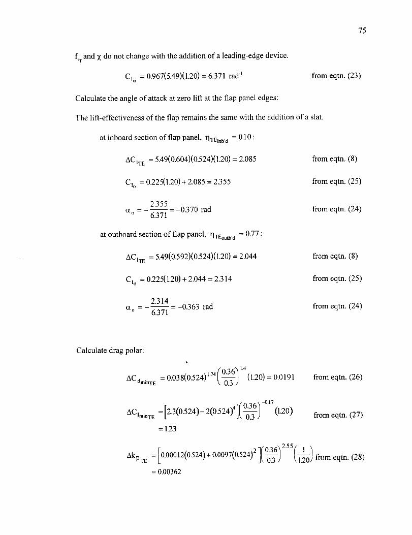
fcfandZdonot changewith theadditionof a leading-edgedevice.
C,_ = 0.967(5.49)(1.20)= 6.371rad"
Calculatetheangleof attackatzerolift attheflappaneledges:
Thelift-effectivenessof theflap remainsthesamewith theadditionof a slat.
atinboardsectionof flappanel, qTEinb, d = 0.10:
AC,T E = 5.49(0.604)(0.524)(1.20)= 2.085
Cio = 0.225(1.20) + 2.085 = 2.355
2.355--0.370 rad
°t° - - 6.371
at outboard section of flap panel, qTZoutb'a = 0.77:
ACIT E = 5.49(0.592)(0.524)(1.20)= 2.044
Cto = 0.225(1.20) + 2.044 = 2.314
2.314--0.363 rad
°t° - - 6.371
from eqtn. (23)
from eqtn. (8)
from eqtn. (25)
from eqtn. (24)
from eqtn. (8)
from eqtn. (25)
from eqtn. (24)
75
Calculate drag polar:
AC dminTE = 0.038(0.524) 1"74(0"36_ 1'4\ 0.3;
(1.20)=0.0191 from eqtn. (26)
AflminTE = [2.3(0.524)- 2(0.524) 4 ]( 0"36/-0.17\ 0.3)
= 1.23
(1.20)from eqtn. (27)
Akp TE = [0.00012(0524) +
= 0.00362
0.0097(0.524) 2 1(03612"55( 1 _)_1\--_-) \ 1.--_J from eqtn. (28)

ACdminLE = 0.0074(1.20) = 0.0089
mCiminTE = 0.76(1.20) = 0.91
AkpLE = 0.00381(_-_)
Cdmi n
Clmi n
= 0.00318
= 0.0067(1.20) + 0.0191 + 0.0089 = 0.0360
= 0.225(1.20) + 1.23 + 0.91 = 2.41
kp= 0.0038(1_) +0.00362+0.00318 = 0.00997
C%rotUe = 0.0360 + 0.00997(C I - 2.41) 2
76
from eqtn. (32)
from eqtn. (33)
from eqtn. (34)
from eqtn. (35)
from eqtn. (36)
from eqtn. (37)
from eqtn. (38)
Calculate pitching moment about the aerodynamic center:
Xcp- 0.400
C t
0LE = COS-I[1- 2(0.145)] = 0.781 rad
1 sin(0.781)[1-cos(0.781)] =-0.102 rad 1CmSL E ---2
= -0.102(0.524)(120) 2 = -0.0770mE mo LE
at inboard section of flap panel:
ACmT E = 2.085[0.25 -- 0.400(1.20)]= -0.480
C mo= -0.06(1.20)2 _ 0.480 - 0.0770 = -0.643
from eqtn. (41)
from eqtn. (44)
from eqtn. (43)
from eqtn. (42)
from eqtn. (40)
from eqtn. (39)

77
at outboardsectionof flappanel:
AC = 2.04410.25-0.400(1.20)]=-0.470 from eqtn. (40)roTE
Cmo = -0.06(1.20) 2 - 0.470 - 0.0770 -- -0.633 from eqtn. (39)
Calculate maximum sectional lift:
AC,m_,TE = 3.786(0.524X1.20)= 2.381 from eqtn. (61)
A(Xmax =0.023+ 1.7(0.145)-1.8(0.145) 2 - 7.3(0.145) 3 from eqtn. (60)= 0.209
AC = 6.371(0.209)= 1.332 from eqtn. (59)ImaxLE
Cim _ = 1.575(1.20)+ 2.381 + 1.332 = 5.60 from eqtn. (58)
This information is insufficient to determine the optimum high-lift system, so the
weight and cost data is calculated next.
Calculate weight and cost of trailing-edge flap:
CTEinb,d = 0.36c inb'a
= 0.36c root
= 0.36 AR
2 jl000= 0.36 1+ 0.25 _/ 8.5
= 6.248 ft

78
CTEoutb, d = 0.36Coutb, d
= 0.36c rootI 1 -
"3
rlTE°utb'd -- rlr°°t (1 -- L)/
d1 - rl root
= 0.36 1 -lqTEoutb,d -- 1"1root
1 - r I root
J 0.77 - 0.1 ]2 1000Ii (1-0.25)
=0"361+0.2---_V 8.5 L 1-0.1
= 2.759 ft
b
STE =(CTEinb,d +CTEoutb,d)1]TE2 -
= (C TEinb,d + CTEoutb,d )Yl TE "q/-_" AR2
= (6.248 + 2.759)0.67 41000(8"5)2
= 278.2 ft 2
Since ffow=l, equation (72) reduces to:
WTE =(al +a2 +a3 +a4)STE
WTE = 8.9(278.2) = 2476 Ib
PCTE = 1610
COStTE = 1.8881(2476)(1610) 0.7 = $ 0.821× 10⁶
Calculate weight and cost of slat:
CLEinb, d = 0.145Cinb, d = 0.145Croot
= 0"1451--_- AR
: q ao= 0145 1 +0.25 _/ 8.5
= 2.516 ft
from eqtn. (80)
from eqtn. (79)

79
C LEoutb, d = 0.145C outb, d
I 1] LEoutb,d -- FI root 1= 0.145Croot 1-- i__ 7o_ (1--)_)
= 0"145 1 +9_ _/AR L 1- rlroot
=0"1451+0.25_/ 8.5 L
= 0.692 ft
b
SLE =(CLEinb,d +CLEoutb,d)TILE 2 -
=(CLEi,b,d +CLEoutb'd)tie E _.AR2
= (2.516 + 0.692)0.87 x/1000(8.5)2
= 128.7 ft 2
Equation (78) can be expressed as:
WEE =(a5 +a 6 +a7)SLE
WLE = 15.3(128.7) = 1969 lb
PC LE = 3100
COStLE = 1.7339(1969X3100) 0.7 = $ 0.949 x 10⁶
from eqtn. (81)
from eqtn. (79)
A summary of the results is shown in tables 10.1 and 10.2 and figures 10.1 and 10.2

80
Single-Slotted Single-Slottedwith3 PositionSlat
1.38CLo 1.28
CD(Or=0°) 0.0953 0.1228
CL..... 1.95 3.03
_max,deg 9.32 21.1
Table 10.1 AerodynamicPerformanceof aSingle-SlottedFlapWith aTrackSupport(With andWithouta Slat)
Single-Slotted 3 PositionSlat Total
SystemWeight,lb 2476 1969 4445
SystemCost,$ 0.821x 10⁶ 0.949x 10⁶ 1.770x 10⁶
Table 10.2 SystemWeightandCostDataof aSingle-SlottedFlapWith aTrack Supportanda SlatWith SlaveTracks

81
Flaps
Flaps+ Slats-- Clean
3.5
3
2.5
CL 2
1.5
0.5 _
-2O I0 20 30
Ct
Figure 10.1 Lift Curves of Sample Test Cases
CD
0.4_
0.35
0.3
0.25 "
0.2
0.15
0.1 '
0.05
0'
/
/
/
Flaps ]- Flaps + Slats
-- Clean
0.5 1 1.5 2 2.5
CL
Figure 10.2 Drag Polars of Sample Test Cases
3 3.5

11.0 Concluding Remarks
82
Today's highly competitive market necessitates the ability to develop a high-lift
system that allows a civil transport aircraft to meet the stringent FAR Part 25 takeoff and
landing requirements with minimal direct operational cost. This presents a daunting task
for designers, since the optimization of a high-lift system is extremely complex. This
report presents a comprehensive design methodology which includes aerodynamic
performance, structural weight considerations, system complexity, and cost to be used
within an aircraft conceptual design tool such as ACSYNT. Thus, aircraft performance
and cost can be analyzed in parallel to select the optimal configuration.
Similar methodologies have been created in the past, but they should not be used
today for two reasons. The methods generally consist of outdated experimental data, and
the data is based on low Reynolds numbers. Today, CFD offers the best alternative,
since it would be too costly to generate a large high-Reynolds-number experimental
database as was done in the past. Computational methods can accurately, yet
inexpensively, predict the flow field around multi-element airfoils in a reasonably short
period of time. However, the most important advantage of using CFD is that airfoils can
be analyzed at realistic flight Reynolds numbers.
CFD was the primary tool used in this research project to construct a database
consisting of the NLR-7301 two-element and the Douglas LB-546 three-element airfoils.
However, supplemental configurations such as a double-slotted and triple-slotted flap

83
mustbeaddedto builda morecomprehensivedatabase.Thiscanbedonewithout
difficulty, sincethenewdesignmethodologyis easilyextensible.
Fromthis databaseempiricalequationswereconstructedwhich areusedto
calculatetwo-dimensionalaerodynamiccoefficients.A spanwiselift distributionis then
determinedfrom a modifiedlifting-line theoryusingthetwo-dimensionaldataasinput.
Thusthetotal lift, drag,pitchingmoment,andmaximumlift of thewing canbecomputed
fasterthanwith apanelmethodwhile incorporatingtheviscouseffectsof slottedhigh-lift
devices.
Sincethedesignmethodologywasintendedto beusedin anoptimizationroutine,
areasonablecompromisebetweenCPUrequirementsandtheaccuracyof thepredictions
hadto be found. Consequently,someassumptionsandsimplificationsweremade. One
suchsimplificationrestsin thepredictionof weightusinghistoricaldata. Although this
techniqueoffersaconsistentapproachfor predictingweight,it is avery simplemethod.
Furtherresearchshouldbeconductedto considera methodwhich incorporatesloading
informationfrom CFDwith slenderbeamanalysisto determinetheoptimalweightof a
configuration.
This methodologyalsoneglectsspanwiseviscousflow effectssinceit employsa
modified lifting-line method.Clearly,thisproblemcannotbesolveduntil full 3-D
viscousflow solutionsbecomepractical.Usingthethree-dimensionalReynolds-averaged
Navier-Stokes(RaNS)equationswill notonly accountfor spanwiseeffects,but will also
allow for inversewingdesign.Nevertheless,until the3-DRaNSequationsfor multi-
elementwingsat high-lift conditionscanbesolvedin areasonabletime period(i.e. less

84
thana day)themethodologypresentedin thispaperwill beausefultool in the
development of high-lift systems on civil transport aircraft.

85
References
2
4
5
6
7
10
11
Smith, A. M. O., "Aerodynamics of High-Lift Aerfoil Systems," in Fluid Dynamics
of Aircraft Stalling, AGARD CP102, Nov. 1972, pp. 10/1-27.
Smith, A. M. O., "High-Lift Aerodynamics," Joumal of Aircraft, Vol. 12, No. 6, June
1975, pp. 501-530.
Garner, P. L., Meredith, P. T., and Stoner, R. C., "Areas for Future CFD
Development as Illustrated by Transport Aircraft Applications," AIAA Paper 91-
1527-CP, June 1991.
Myklebust, A. and Gelhausen, P., "Putting the ACSYNT on Aircraft Design,"
Aerospace America, Sept. 1994, pp. 26-30.
Woodward, D. S. and Lean, D. E., "Where Is High-Lift Today? - A Review of Past
UK Research Programmes," in High-Lift System Aerodynamics, AGARD CP-515,
Sept. 1993, pp. 1/1-45.
Wedderspoon, J. R. "The High Lift Development of the A320 Aircraft," ICAS 86-
2.3.2, September 1986.
Flaig, A. and Hilbig, R., "High-Lift Design for Large Civil Aircraft," in High-Lift
System Aerodynamics, AGARD CP-515, Sept. 1993, pp. 31/1-12.
Rogers, S. E., Wiltberger, N. L., and Kwak, D. "Efficient Simulation of
Incompressible Viscous Flow Over Single- and Multi-Element Airfoils," Journal of
Aircraft, Vol. 30, No. 5, Sept., 1993, pp. 736-743.
Rogers, S. E. and Kwak, D., "An Upwind Differencing Scheme for the Steady State
Incompressible Navier-Stokes Equations," Journal of Applied Numerical
Mathematics, Vol. 8, 1991, pp. 43-64.
Coa, H. V. and Kusunose, K., "Grid Generation and Navier Stokes Analysis for
Multi-Element Airfoils," AIAA Paper 940748, Jan. 1994.
Mavriplis, D. J., "Turbulent Flow Calculations Using Unstructured and Adaptive
Meshes," NASA CR 182102, Sept. 1990.

86
12 Mavriplis, D. J., "UnstructuredMeshAlgorithmsfor AerodynamicCalculations,"inFifth SymposiumonNumericalandPhysicalAspectsof AerodynamicFlows,Califomia StateUniversity,LongBeach,CA, Jan.1992.
13 Valarezo,W. O.andMavriplis, D. J., "Navier-Stokes Applications to High-Lift
Airfoil Analysis," AIAA Paper 933534, Aug. 1993.
14 Drela, M., "Newton Solution of Coupled Viscous/Inviscid Multi-Element Airfoil
Flows," AIAA Paper 90-1470, June 1990.
15 Hardin, J. D., Potter, R. C., van Dam, C. P., and Yip, L. P., "Two-Dimensional
Computational Analysis of a Transport High-Lift System and Comparison with
Flight-Test Results," AIAA Paper 93-3533, Aug. 1993.
16 Rogers, S. E., Menter, F. R., Durbin, P. A., and Mansour, N. N., "A Comparison of
Turbulence Models in Computing Multi-Element Airfoil Flows," AIAA Paper 94-
0291, Jan. 1994.
17 Vinh, H., van Dam, C., Yen, D., and Pepper, R., "Drag Prediction Algorithms for
Navier-Stokes Solutions About Airfoils," AIAA Paper 95-1788, June 1995.
18 van den Berg, B., "Boundary Layer Measurements on a Two-Dimensional Wing with
Flap," National Aerospace Laboratory TR-79009 U, The Netherlands, January 1979.
19 Lin, J. C. and Dominik, C. J., "Optimization of An Advanced Design Three-Element
Airfoil at High Reynolds Numbers," AIAA Paper 95-1858, June 1995.
20 Lean, D. E. and Fiddes, S. P., "A Rapid Method for Estimating Equivalent Parabolic
Polars from Wind-Tunnel Test," RAE Tech. Memo AERO 2034, April 1985.
21 Kusunose, K. and Cao, H., "Prediction of Transition Location for a 2-D Navier-
Stokes Solver for Multi-Element Airfoil Configurations," AIAA Paper 94-2376, June
1994.
22 Weissinger, J., "The Lift Distribution of Swept-Back Wings", NACA TM 1120,
1947.
23 Hoak, D., "USAF Stability and Control Datcom", Flight Control Division, Air Force
Flight Dynamics Laboratory, WPAFB, Ohio, 45433-0000, 1978, revised.
24 Schlichting, H. and Truckenbrodt, E., Aerodynamics of the Airplane, McGraw-Hill,
1979.

87
25
26
27
28
29
3O
31
32
33
34
35
36
37
Roshko,A. "Computationof theIncrementof MaximumLift Dueto Flaps,"DouglasAircraft Co.Report SM-23626,1959.
Moran,J.,An Introduction to Theoretical and Computational Aerodynamics, John
Wiley & Sons, 1984.
Holbrook, G. and Dunham, D., "Detailed Pressure Distribution Measurements
Obtained on Several Configurations of an Aspect Ratio-7 Variable Twist Wing,"
NASA TM 86308, 1985.
Hunton, L. W., "Effects of Twist and Camber on the Low-Speed Characteristics of a
Large-Scale 45 ° Swept-Back Wing," NASA RaM A50A10, 1950.
Valarezo, W. and Chin, V., "Method for the Prediction of Wing Maximum Lift,"
Journal of Aircraft, Vol. 31, No. 1, Jan. 1994, pp. 103-109.
Ljungstr/Sm, B. L. G. "Two-Dimensional Wind Tunnel Experiments with Single and
Double Slotted Flaps," FFA Technical Note AU-1083, Oct. 1975.
Murillo, L. and McMasters, J., "A Method for Predicting Low-Speed Aerodynamic
Characteristics of Transport Aircraft," Journal of Aircraft, Vol. 21, No. 3, March
1984, pp. 168-174.
Vanderplaats, G., Numerical Optimization Techniques for Engineering Design: with
Applications, McGraw-Hill, 1984.
Anderson, R., Flora, C., Nelson, R., Raymond, E., and Vincent, J., "Development of
Weight and Cost Estimates for Lifting Surfaces with Active Controls," NASA CR-
144937, March 1976.
Oman, B. H., "Vehicle Design Evaluation Program," NASA CR-145070, Jan. 1977.
Anderson, R., Flora, C., Nelson, R., Raymond, E., and Vincent, J., "Development of
Weight and Cost Estimates for Lifting Surfaces with Active Controls," NASA CR-
144937, March 1976.
Ardema, M. et al., "Analytical Fuselage and Wing Weight Estimation of Transport
Aircraft," Oct. 1995.
Yip, L. P., et ai., _ i'he NASA B737-100 High-Lift Research Programme-
Measurements and Computations," Aeronautical Journal, Nov. 1995, pp. 372-386.
38 Gelhausen, P., Personal Communication, Jan. 1996.

88
39 Rudolph,P.,PersonalCommunication,Sep.1995.
40 Anon., "Simpler737FlapDesign,"Aviation Week& SpaceTechnology,April 18,1994,p. 38.

89
Appendix A
Spanwise Load Distribution Calculations of a Wing with
Arbitrary Plan Form Using the Weissinger Method
Summary
The application of Weissinger's theory is shown for calculating the spanwise
loading across a wing. From this procedure a spanwise load distribution can be
calculated for a wing of arbitrary plan form from a 2-D lift curve slope and angle of zero
lift. The geometry of the wing may be asymmetric about the centerline and can include
sweep, taper, or twist. Partial span flaps may be modeled as discontinuities in twist.
Fowler motion can also be modeled as an increase in chord length. Lift, induced drag,
pitching moment, and induced angle of attack may then be calculated.
Method
The Weissinger method models the wing as a plate of zero thickness, but the
planform and twist remain identical to the actual wing. The chordwise load distribution
at each span station is concentrated into a lifting line located at the wing's quarter-chord
line. The theory requires that the quarter chord line is straight, however a discontinuity is
allowed at the plane of symmetry so that a swept wing may be considered.
The method assumes that the lifting line and its trailing vortex sheet are
continuous. However, discrete values for the circulation strength are determined only at
the span stations along the quarter-chord line corresponding with control points. The

90
numberof controlpoints,m, is specified,andeachis placedatthethree-quarter-chord
line. Mathematicallythis impliesthatthe lift curveslopeis2n rad -1, and a correction
method must be incorporated for a lift curve slope that varies from the theoretical value.
The boundary conditions specify that the induced angle of attack due to the
downwash of the trailing vortex is equal to the angle of attack of the plate. This ensures
tangency of the flow to the plate at each control point.
Substituting the wing with a bound vortex system and applying the boundary
conditions enables the formation of a set of simultaneous equations. Each of these
Ctc
equations is a function of the angle of attack of the wing, the load coefficient Gj - 2b
at each span station j on the quarter-chord line, and the influence coefficients A_j which
are only a function of geometry and relate the influence of the circulation at any point j
along the lifting line to the downwash at any control point i. The distribution of the load
Gj may then be calculated from the set of m simultaneous equations.
m
_i = EAi,jGj , i = 1,2,3 .... mj=l
(A-I)
where
W i
(_i -- Vo ° - (Of.wing - (3£ o )i (A-2)
Each equation gives the downwash angle at the control point rl = cosd_i resulting from
the circulation effects of m points along the span.
The following trigonometric substitutions are used to define span locations at the
control points or on the lifting line respectively,

_ _hA. _ ....
C_

91
(A-3)
(A-4)
.... :ients are shown below.
(A-6)
?
- --gi,j (A-7)
:_i 1-(-1) j-i
-.os_i) 2 2(m+l)(A-8)
--_nts are given as
_-i,ofj,o + Ci,M+lfj,M+ 1
2
M
+ _--' Li.k fj,k) (A-9)k=l
.... of span stations used to integrate the downwash and does not have
- - L The subscripts 0 and M+ 1 denote values for k. Also note that
=j (A-10)
coefficients L_,k are defined as follows:
(A-',:)

92
kT_
m+l(A-12)
for __< 0
1 _/[1 + (b / c)( rl + q) tanA]2 + (b / c)2 (rl - q) 2
Li'k (b/c)(rl-7) {= 1 +(b/c)(rl + q)tanA
2tanA_/[1 + (b / c) r1 tanA] 2 +(b/c)Zq 2+
[l+(b/c)(r I -q)tanA][l+(b/c)(r I +q)tanA]
-1}
(A-13)
for _>_0
1Lik = {
'X/[1 + (b / c)([rl]- q)tanAl 2 + (b / c) 2 (r I - _)2
1 + (b / c)([rll- rl)tanA-1}
(A-14)
The mathematical series coefficients fj.k are used in a numerical integration method and
are shown below:
kT_(A-15)
d_k = COSM+ 1
2 m
fjk -- _--_ktsin _tqbj c°s kt_bk' m+l_=_
(A-16)
Sectional Lift curve Slope Correction
The Weissinger method assumes that the lift curve slope is 27_ rad -I . This implies
that the control points lie along the three-quarter-chord line. When considering airfoils
with lift curve slopes that vary from this theoretical value (as a result of viscous,
compressibility, or geometry effects), a correction method must be incorporated. This

93
involvesmovingthecontrolpointsfrom thethree-quarter-chordline; butbeforethis is
donea derivationof this locationwill beshown.
Thevelocity inducedby aninfinite vortexof strengthF anddistanceh isgivenas
Fw - (A-17)
2nh
andthesectionallift coefficientis relatedto thecirculationstrengthasfollows:
1 2
pVooF = _ pVoocCi
Rearranging these two equations and combining them yields
whC I = 4n
Vo_ c
(A-18)
(A-19)
w
Since ot = _ the above equation can be rewritten as
C t h- 4n- (A-20)
(_ C
h 1If the lift curve slope is assumed to be 2n then it can be shown that - must be c Thenc 2 "
1
the point at which no flow passes through the plate occurs at -_ c from the lifting line or
at the three-quarter-chord line.
If the lift curve slope deviates from the theoretical value each control point
location must be modified. This means that each control point must be moved forward of
the three-quarter-chord line if the slope is less than 2n rad -1 or must be moved rearward if
bit is greater. This variation can also be modeled as a change in the value of -- by the
Cv

94
ratio of the experimental lift curve slope to the theoretical lift curve slope --C icXcxp
2 /13at the
desired Mach number, M, where 13= x/i-- M 2 . The modified geometry can be expressed
as
b b(--) mod = k _ -- (A-21)
Cv Cv
where
C letexp
k_- 2n/]3(A-22)
Caution should be taken when large deviations in the lift curve slope are used. The
method does not rigorously allow such modifications, and the accuracy of the results may
deteriorate for large angles of sweep.
Compressibility Correction
Compressibility effects are included with the aid of the Prandtl-Glauert rule. It
approximates the effects of compressibility as an increase in the local chord and sweep
1angle by the factor -
b 1 b (A-23)-13cv
. -l tanA
AI3 = tan t-if--)(A-24)
Thus the span loading for the original plan form at a given Mach number can be
calculated for an incompressible flow using a modified geometry.

95
Aerodynamic Characteristics
The circulation strength is calculated directly from the dimensionless load
coefficient and has the dimensions [fl2/s].
F v = bV_oG
The sectional lift coefficient is also calculated from the load coefficient as
b
Cl_ =2--GvCv
The total lift coefficient is determined from
reAR _'_Gv sind?_m¥i o,
The induced angle of attack at the quarter-chord point of station v is given by
m
oti_ = b_G_ - _-"/b_nG n
(A-25)
(A-26)
(A-27)
(A-28)
nAR m
Coi -- m---+l _-Gv_iv sin d_vV: l
total induced drag is calculated from
(A-29)
n=l
where the primed summation sign indicates that the value for n = v is not summed. The

Appendix B
96
Weight Estimation of Other Control Surfaces
Like leading and trailing-edge device weights, the estimation of aileron and
spoiler weights is based on historical data of existing aircraft. Similarly, the total system
weights are broken up into components of surface, support, and actuation. The weight
estimation equations given below are only a function of the planform area of the
representative control surface.
Aileron Weight
Surface Weight:
W_urf = 5.5. Sail (B- 1)
Support Weight:
Wsupp = 0.74. Sail (B-2)
Actuation Weight:
Wact = 4.3" Sai I (B-3)
Total Aileron Weight:
Wai t = Wsorf + Wsupp + Wact (B-4)

Spoiler Weight
97
Surface Weight:
Wsurf = 110+ 1.65.Ss0
Support Weight:
Wsupp = 1.3.Ssp
Actuation Weight:
Wact = 270+ 1.35-Ssp
Total Spoiler Weight:
Wsp = Wsurf + Wsupp + Wac t
(B-5)
(B-6)
(B-7)
(B-8)

98
Appendix C
High-Lift Weight Data of Various Aircraft
(All weights are in pounds.)
Traillng-Edge Device Weight Data
Weight Boenag 727-200 Boeing 737-200 Boeing 747-2 I P Boellg 757-200 Boemg 767 DC-8 Model O2F NE)-83 MD- I 1
Sarfa_ f,57 _,_ I 1_ ]53 432 785 2491 1713 5516 1518 _g_2 842 18_kl gJ 478 2285 129! I_)_ 1885 341_J
• _ppofts 139l 76'_ 17E 411 473 884 516_ 2732 751c_ 1549 1427 979 24_ 98? 83! ]Of_ 191 1816
Fakings 291 51_ 1118 164 1319 (AI 158_ 392 159 170 329 -- -- -- 5¶ 191 213
Contmb 9"- 722 21"_: 722 -- -- 3_ 24] 977
Total 412- 2555 Ib78_ 4181 ]_I 1_1 631_
17%A
Nk_lted Ate& S-m 28: 175 84_ 327 173 236 4_) 4509' 2101 f_2
Wdght / S_
Satiate 4 2t, i 4 49 651 464 5.56 357 44l 5Ill, 6 I! 5/.2
SuppoNs 606i 505 #85 474 825 4 i5 588 233 (19a 272
C)anlgol. i 12! 4 13 25( 221 081 I 14 (18_
Total I 4 68, 14 (_) 19 8_ 1239 8 14 8 4_ 9 44
Ltadlng-Edge Device Weight Data
Weight Boell_ 727-200 B_ein 8 737-200 Boe mlg 747-21P Boem 8 757-200 Boeing 767 DC-8 Model 62F MD-83 MD- 11
"'-_ I..... t .......... I...... I ........ I..... I ........ I..... I ......... t..... I ......... I..... q ......... q.... I ....... I.... I '_25_ "_H 752 I27 272 597 652 652l 423 1591 2/114Sudao_ 3')9 37_ I1_; 150'_ 5'): {)
Suppoll 214 214 It I(X) I(X) t)l: "_1_
Conlro[s _48 232 t25_
total t 314 731 ] 555
Nested Area. Su_ 55 14! 2{x) 24 3 76 3 100.6 12_ 32(
SuJfaoe 455 34_ 37(, 523 356 397 311 34_ 33_
01_ I_ 107 Oflh ]31 099 1)74 2.1_ 171
Coatlmb 174 -- -- 231 27%
Total {, 57 727 7 _)_
Iqzed Structure Weight Data
I Weight 13-727 U-737 B-747 13-757 []-767 DC-_ MD43 MD-II
Tr_tg Edge 648 37_) 1833 1351 871
I ,.-_ting Edge 817 4_12 _l(X) yr7 2213
Aileron Weight Data
Weight [3-727 B-717 13-747 []-757 B-767 IX'-8 MD41 MD-II
S*udac_ 34. 137 'A_ 25Jt_ 359 I3 1(}2]
Suppect 4_ 16 Ifd, 3861 2295!
Chat I_*lt 29 226 IIX_) 42_ 1097_ 5P,2_
Ailk_O0 At¢_. S.,* _7 2(I 9 226 48 1246 i6l_ 3_ 1871
SUp_OflS 07_I 1159 073 0()] lO_ I_
Contmb 5111 8411 446 264 28% 3 It
Spoiler Weight Data
Wetght B-727 I [3-717 [3-747 [3-757 1]-767 IX. "_g MD-_3 MD-]I
_.faoe 33; 156 582 33'
391 ]32. T, 1751_
Total 71); -146 1(,53 4fdl 5! 11135 9_
l°._t ted Area. S,p 791 45 I _34 256 r_.4 4g_ _ M : lY
Wdghl I S., ISuffaoe 4 [61 3 46 ] 91 o(X 26_
Supports 11013 0 t_l I 29 3 E I 2_
Contmh 576 6 43 2.24 9 4! 361
I_ _6
(I 0 93"_ 937 48_ l&]4 232_
148 I(Xt3: -- -- 1461
745 2592 _rs_
1208 I1( 12fl& 1(I) 3 3716 471_
5_1 -- 5-_) 422 4_ 4.z,
776 -- 776 4_ 494 49_
g]o -- -- 31(

Appendix D
99
Database Formulation
The first step in integrating a database into the high-lift module is to formulate the
data based on important parameters. This has already been done, and the empirical
equations can be found in the documentation. The second step is to determine
appropriate empirical coefficients for the formulas. This has been completed for leading-
edge devices and single-slotted trailing-edge flaps but can be done for other
configurations by finding the empirical coefficients which minimize the error between the
predictions and the actual data. In other words, iterate on the empirical coefficients to
minimize the RMS:
RMS = X/average(predicted values - database values) 2
The empirical equations for Z, ACdmi n, ACImi n, mkp, Cis,nax, and Xcp are given in equations 11,
26, 27, 28, 62, and 41 respectively and must be fit to a new configuration data set in order
to integrate the new configuration. The database values of these parameters are
determined from the CFD data as follows:
ACITE (Find Z which accurately predicts_8 = C _
C letclean _TE --C
cts.)
ACIT E = C I - Clclean