design methodology and tools in factory of the future

DOI: 10.2478/ijasitels-2021-0001

Design Methodology and Tools in Factory of the Future

FLOREA Adrian1, MIRONESCU Ion1, CRĂCIUNEAN Daniel1, MORARIU Daniel1, VOLOVICI Daniel1

1 Lucian Blaga University of Sibiu, Department of Computer Science, Electrical and Electronical Engineering,

DigiFoF Project Nr. 601089-EPP-1-2018-1-RO-EPPKA2-KA, https://digifof.eu/

{adrian.florea, ion.mironescu, daniel.craciunean, daniel.morariu, daniel.volovici}@ulbsibiu.ro

Abstract

This paper presents a design method and tool developed to support the skill forming activities

in the DigiFoF network (https://www.digifof.eu/). The focus is on training of manufacturing

system design skills both as HEI education and vocational training, but preliminary design of new manufacturing systems is also supported (e.g in the development of small business

process scenarios).

We proposed a model-based methodology for solving of the manufacturing system design

problems The methodology and the supporting tool are centred around a less abstract Domain-

Specific Modelling Language (DSML). The language is easy to learn due to its few components.

A modelling and simulation environment named Digital Production Planner Tool (DPPT) was

generated from the metamodel of the DSML. The degree of abstraction used by this tool

corresponds well to the intended use in training and preliminary design.

Our method incorporates by design the possibility to impose constraints at the modelling language level to limit the modelling space to feasible/possible solutions. The resulting tool

enforces these constraints in the use and supports the development of feasible designs even by

inexperienced designers.

The access to the conceptual model allows the translation of the model to other modelling

language like Petri net. This extends the support for the design methodology.

The whitepaper presents a use case for the developed method and tool: the design of a

chocolate manufacturing line.

Keywords: ADOxx modelling, Factory of the Future, Internet of Things,

1 Introduction

A study based on the answers of 108 employees (of different job categories) from 6 European countries (Romania, Poland, Italy, France, Germany, and Finland), 67% of them working in medium, large and very large enterprises, analyzed the design skills required by employees, how firms provide training for their employees, which is the level of innovation in the industry [DigiFoF2019]. The results of the research confirm the significant role of possessing and building digital designing knowledge and skills among present and potential employees of

3

https://digifof.eu/

https://www.digifof.eu/

International Journal of Advanced Statistics and IT&C for Economics and Life Sciences December 2021 * Vol. XI, no. 1

© 2021 Lucian Blaga University of Sibiu

manufacturing companies. The level of competence in the analyzed group of companies is not satisfactory in this field. The following is a summary of the main findings from the survey:

• importance of digital design skills in companies. • not sufficient level of companies’ ability in trainings for FoF. • knowledge gap exists in the scope of advanced methods and tools supporting

the development of innovative products and services. • respondents recognize the need to improve them mainly through organization

and participation in additional internal trainings. • enterprises are interested in process modelling and it is perceived as

fundamental for the optimization and redesigning processes in enterprises. • a lack of skills or a lack of access to necessary infrastructure supporting process

modelling and model-based designing for cyber-physical systems. • lack of practical experience with enterprise architecture management, business

modelling and digital mock-ups. • low/moderate level of process digitalization in enterprises. • low or moderate levels of process automation and control.

Due to the identified lack of experience and knowledge in this area, training on digital designing should be conducted systematically and adapted to the conditions of business operations. To improve the digital design skills, the DIGIFOF project has developed a network of training environments where HEIs, enterprises and training institutions come together to develop skill profiles, training concepts as well as materials for design aspects of the Factory of the Future (FoF). This structure foster knowledge transfer between industry and academia, aiming to provide educational and experimental OMiLAB4FoF laboratories, where FoF-aspects can be taught practically or experimented with. In this skill development environment, design is understood as the process of novel business models creation and assessment within an experimentation space. [Karagiannis2020]

This whitepaper presents a design method and tool developed to support the skill forming activities in the DigiFoF network. The focus is on training of manufacturing system design skills both as HEI education and vocational training, but preliminary design of new manufacturing systems is also supported (e.g., in the development of small business process scenarios).

1.1 Intended scope

Only flexible manufacturing systems (FMS) can respond to the rapid changes of a demanding market. Such manufacturing systems can produce multiple types of products by providing the possibilities of reconfiguring. This reconfiguration can be performed rapidly to respond to the dynamic of the market. An FMS consist of:

• a set of workstations capable of the automatic execution of large sets of operations. This defines the machine flexibility and helps the FMS to cope with large-scale changes in volume, capacity, or capability demands.

4



• a material handling system flexible conveyor, automated guided vehicles (AGV) and loading-unloading robots - routing flexibility changed to produce new product types, change the order of operations.

• a complex command and control system - orchestrates the cooperation. From a design perspective a description of the FMS should also include, in an abstracted form the knowledge about its capabilities. This knowledge is the answer to some questions that can be reformulated in requirements for a design problem: What raw material it can intake? What transformation it can apply to these materials? At which parameters? What can it produce and with wat yield? This knowledge is a very important support for the design approach.

1.2 An illustrative example - a chocolate production line

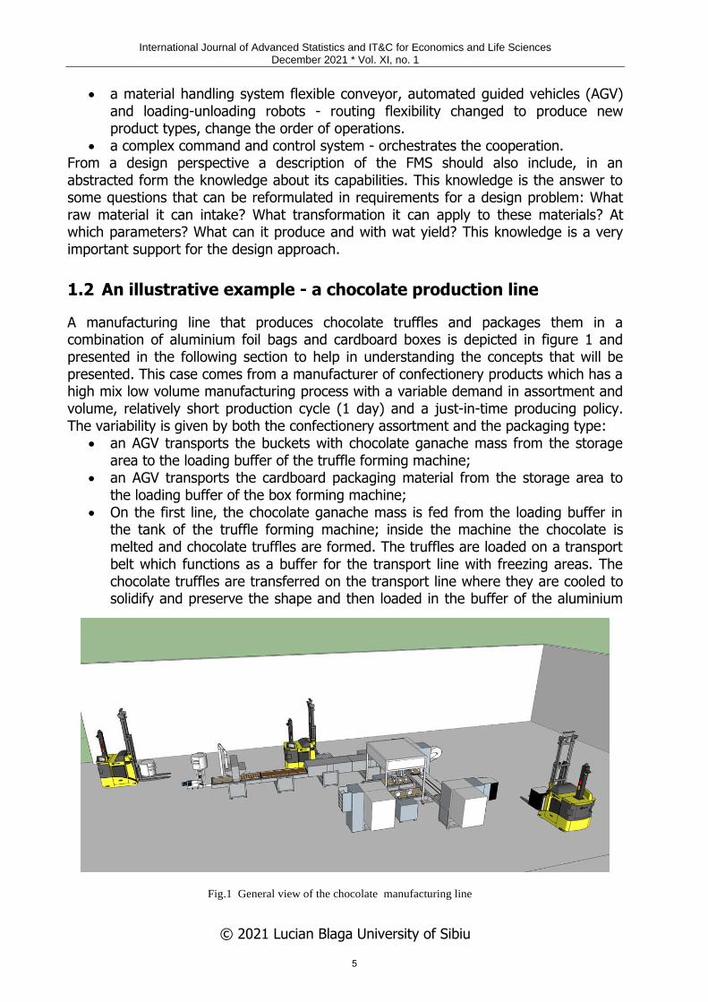
A manufacturing line that produces chocolate truffles and packages them in a combination of aluminium foil bags and cardboard boxes is depicted in figure 1 and presented in the following section to help in understanding the concepts that will be presented. This case comes from a manufacturer of confectionery products which has a high mix low volume manufacturing process with a variable demand in assortment and volume, relatively short production cycle (1 day) and a just-in-time producing policy. The variability is given by both the confectionery assortment and the packaging type:

• an AGV transports the buckets with chocolate ganache mass from the storage area to the loading buffer of the truffle forming machine;

• an AGV transports the cardboard packaging material from the storage area to the loading buffer of the box forming machine;

• On the first line, the chocolate ganache mass is fed from the loading buffer in the tank of the truffle forming machine; inside the machine the chocolate is melted and chocolate truffles are formed. The truffles are loaded on a transport belt which functions as a buffer for the transport line with freezing areas. The chocolate truffles are transferred on the transport line where they are cooled to solidify and preserve the shape and then loaded in the buffer of the aluminium

Fig.1 General view of the chocolate manufacturing line

5



foil packaging machine. Two processes occur here: the formation of the bags from the aluminium foil taken from a roll and the filling of the aluminum bags with chocolate truffles. The resulted aluminum bags filled with chocolate truffles are buffered in a dispenser;

• On the second line, cardboard packaging material from the loading buffer, is transformed by the box forming machine in cubic cardboard boxes. The boxes are loaded in the machine output buffer;

• On the assembly line, a robotic arm transfers alternatively the aluminium bags and the cardboard boxes on the feeding transport belts which function as a buffer for the final packaging machine. The packaging machine has a robotic arm with flex gripper that introduces the aluminum bags with truffles in the cardboard boxes. The final product - cardboard boxes having aluminum bags with truffles - is discharged in a storage buffer from which it is then later transported to the finite product storage area.

1.3 Design problem

In this context a design problem consists in finding the right and optimal configuration of such a system that can respond to a customer order. A customer order specifies an assortment of products characterized by type of material and quantity that must be produced under some time and cost constraints. It can be a design-from-scratch problem for a new facility or a redesign/reconfiguring problem for an existing facility. A solution to a design problem has two aspects:

• one structural o the components of the manufacturing line o their spatial placing o their fixed and dynamic connections

• one organizational o the order and the timing in which the processed parts are entering each

component of the production line. Due to the complexity of this activity and due to the digital nature of the control and command system the design must be also digitalized or supported by digital tools.

1.4 Requirements for the design tool

We intend to design a methodology and a tool that is not only able to generate a solution for the design problem – a system that corresponds to the user needs expressed in the design requirements. It also should emphases the capabilities of the designed system in manner that allows an innovative use (transformative, disruptive, new business model), The assessment of this capabilities should be possible already during design. This requires Model Driven Engineering as development methodology. Challenge: how to design a system that a) corresponds to the user needs, b) reflects the capabilities in an innovative manner (transformative, disruptive, new business model) and c) provides assessments results already during design The design activity should be divided in three sub-activities presented below (A1-A3) [Mironescu2020].

6



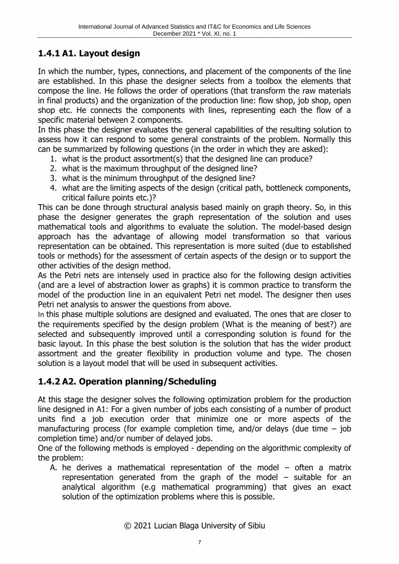
1.4.1 A1. Layout design

In which the number, types, connections, and placement of the components of the line are established. In this phase the designer selects from a toolbox the elements that compose the line. He follows the order of operations (that transform the raw materials in final products) and the organization of the production line: flow shop, job shop, open shop etc. He connects the components with lines, representing each the flow of a specific material between 2 components. In this phase the designer evaluates the general capabilities of the resulting solution to assess how it can respond to some general constraints of the problem. Normally this can be summarized by following questions (in the order in which they are asked):

1. what is the product assortment(s) that the designed line can produce? 2. what is the maximum throughput of the designed line? 3. what is the minimum throughput of the designed line? 4. what are the limiting aspects of the design (critical path, bottleneck components,

critical failure points etc.)? This can be done through structural analysis based mainly on graph theory. So, in this phase the designer generates the graph representation of the solution and uses mathematical tools and algorithms to evaluate the solution. The model-based design approach has the advantage of allowing model transformation so that various representation can be obtained. This representation is more suited (due to established tools or methods) for the assessment of certain aspects of the design or to support the other activities of the design method. As the Petri nets are intensely used in practice also for the following design activities (and are a level of abstraction lower as graphs) it is common practice to transform the model of the production line in an equivalent Petri net model. The designer then uses Petri net analysis to answer the questions from above. In this phase multiple solutions are designed and evaluated. The ones that are closer to

the requirements specified by the design problem (What is the meaning of best?) are selected and subsequently improved until a corresponding solution is found for the basic layout. In this phase the best solution is the solution that has the wider product assortment and the greater flexibility in production volume and type. The chosen solution is a layout model that will be used in subsequent activities.

1.4.2 A2. Operation planning/Scheduling

At this stage the designer solves the following optimization problem for the production line designed in A1: For a given number of jobs each consisting of a number of product units find a job execution order that minimize one or more aspects of the manufacturing process (for example completion time, and/or delays (due time – job completion time) and/or number of delayed jobs. One of the following methods is employed - depending on the algorithmic complexity of the problem:

A. he derives a mathematical representation of the model – often a matrix representation generated from the graph of the model – suitable for an analytical algorithm (e.g mathematical programming) that gives an exact solution of the optimization problems where this is possible.

7



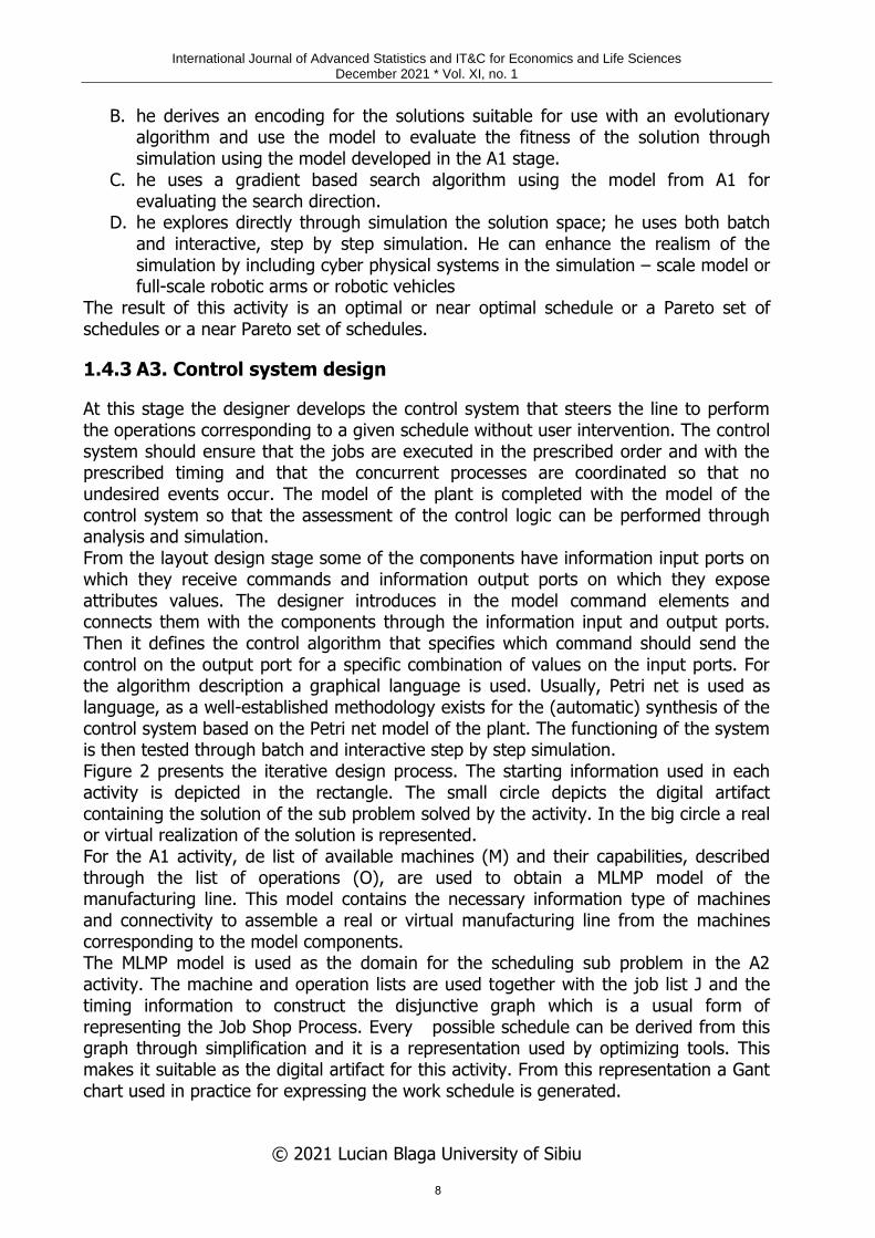
B. he derives an encoding for the solutions suitable for use with an evolutionary algorithm and use the model to evaluate the fitness of the solution through simulation using the model developed in the A1 stage.

C. he uses a gradient based search algorithm using the model from A1 for evaluating the search direction.

D. he explores directly through simulation the solution space; he uses both batch and interactive, step by step simulation. He can enhance the realism of the simulation by including cyber physical systems in the simulation – scale model or full-scale robotic arms or robotic vehicles

The result of this activity is an optimal or near optimal schedule or a Pareto set of schedules or a near Pareto set of schedules.

1.4.3 A3. Control system design

At this stage the designer develops the control system that steers the line to perform the operations corresponding to a given schedule without user intervention. The control system should ensure that the jobs are executed in the prescribed order and with the prescribed timing and that the concurrent processes are coordinated so that no undesired events occur. The model of the plant is completed with the model of the control system so that the assessment of the control logic can be performed through analysis and simulation. From the layout design stage some of the components have information input ports on which they receive commands and information output ports on which they expose attributes values. The designer introduces in the model command elements and connects them with the components through the information input and output ports. Then it defines the control algorithm that specifies which command should send the control on the output port for a specific combination of values on the input ports. For the algorithm description a graphical language is used. Usually, Petri net is used as language, as a well-established methodology exists for the (automatic) synthesis of the control system based on the Petri net model of the plant. The functioning of the system is then tested through batch and interactive step by step simulation. Figure 2 presents the iterative design process. The starting information used in each activity is depicted in the rectangle. The small circle depicts the digital artifact containing the solution of the sub problem solved by the activity. In the big circle a real or virtual realization of the solution is represented. For the A1 activity, de list of available machines (M) and their capabilities, described through the list of operations (O), are used to obtain a MLMP model of the manufacturing line. This model contains the necessary information type of machines and connectivity to assemble a real or virtual manufacturing line from the machines corresponding to the model components. The MLMP model is used as the domain for the scheduling sub problem in the A2 activity. The machine and operation lists are used together with the job list J and the timing information to construct the disjunctive graph which is a usual form of representing the Job Shop Process. Every possible schedule can be derived from this graph through simplification and it is a representation used by optimizing tools. This makes it suitable as the digital artifact for this activity. From this representation a Gant chart used in practice for expressing the work schedule is generated.

8



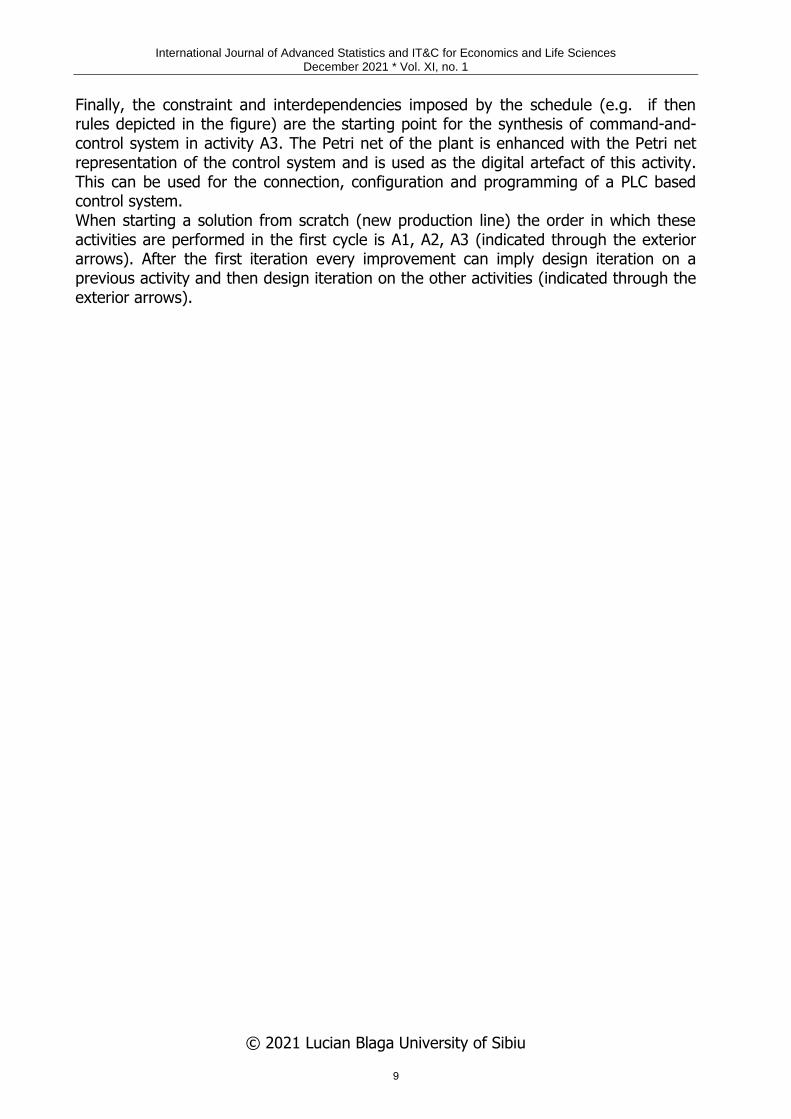
Finally, the constraint and interdependencies imposed by the schedule (e.g. if then rules depicted in the figure) are the starting point for the synthesis of command-and-control system in activity A3. The Petri net of the plant is enhanced with the Petri net representation of the control system and is used as the digital artefact of this activity. This can be used for the connection, configuration and programming of a PLC based control system. When starting a solution from scratch (new production line) the order in which these activities are performed in the first cycle is A1, A2, A3 (indicated through the exterior arrows). After the first iteration every improvement can imply design iteration on a previous activity and then design iteration on the other activities (indicated through the exterior arrows).

9



Fig. 2 Iterative design activity

10



2 A1 The Digital Production Planner

The core of our support environment for the design method is the Digital Production Planner which supports mainly the sub activity A1. The support for modelling and simulating the temporal dimension is not supported in both the Digital Production Planner and ADOxx based Petri net tools. This dimension is especially important for activity A2 but also for activity A3 so that these activities must be supported by external tools. We intend to implicate the ADOxx community in solving this issue so that a better alignment of ADOxx based tools to the methodology can be achieved.

2.1 Methodology

The purpose of this research is to define important steps in the process of optimal development of a tool dedicated to Digital Production Planner, specific to the domain. The process of developing such a tool includes two important steps, namely the specification of the modelling method concept specific to the modelling domain in question and the implementation of this modelling method in a modelling tool. The concept of modelling method specified in this project was called Modelling Method for Digital Production Planner (MM-DPP). The modelling tool that implements the concept MM-DPP, we called it the Digital Production Planner Tool (DPPT) and we implemented it on the ADOxx metamodeling platform. The main component of this tool is the Modelling Language for Manufacturing Processes (MLMP), which we will present in the following. We will define a Modelling Language for Manufacturing Processes (MLMP) designed specifically for specifying and optimizing manufacturing processes. MLMP is a language for modelling manufacturing processes to represent the logical and functional dependencies of the activities of a manufacturing process. The objective of the MLMP language is the conceptual integration of the functional perspective of the manufacturing processes in order to optimize them. The language is addressed to the Digital Production Planner (DPP).

2.2 Formalizing the concept of modelling method

We understand a manufacturing process as a behavior model of a dynamic system at a certain level of abstraction. The behavior of the system is given by several processes that are executed simultaneously (parallel and distributed), where these processes exchange data to influence each other's evolution. The theoretical mechanism most used for modeling processes is the transition system. Transition systems are mechanisms with a well-defined syntax and semantics but become impossible to use in competing systems. For this reason, a lot of other higher-level languages such as Petri Nets, BPMN, EPC, UML, etc. are used in practice. These models describe the processes in terms of activities ordered through casual dependencies [Craciunean2018] [Craciunean2019]. A mechanism that can be the base of such a metamodel is the concept of modeling method.

11



The variety of manufacturing processes, often, makes it necessary to implement specific modelling tools. The first phase of this process is the specification and implementation of the Modelling Method over a metamodeling platform. The language specific to a Modelling Method [Karagiannis2002] relies heavily on graphic elements. To represent the properties of the models in the form of specifications, it is important to build the most appropriate language to enable these specifications to be written in a very clear and simple form. The graphical representation of the formal model provides means for user interaction and model value functionality to process the representation (incl. transformation). A modeling method however is a concept [Karagiannis2002], [Bork2019] that consists of two components: (1) a modeling technique, which is divided in a modeling language and a modeling procedure, and (2) mechanisms & algorithms working on the models described by a modeling language. The modeling language contains the elements with which a model can be described. The modeling procedure describes the steps applying the modeling language to create results, i.e., models. Algorithms and mechanisms provide “functionality to use and evaluate” models described by a modeling language. Combining these functionalities enables the structural analysis, as well as simulation of models. Essentially, a modeling language relies heavily on the graphical notation. The modeling procedure describes the steps to be followed in applying the modeling language to create results, i.e. patterns. Algorithms and mechanisms provide functionality for the use and evaluation of models described by a modeling language. This functionality is given by the processes that act on models to change their state. Combining these functionalities allows structural analysis as well as the simulation of the models. The essential part of a Modeling Method is the modeling language. In our approach, this language is a Domain-Specific Language (DSL). A DSL [Fowler2010] [Karagiannis2016] is a programming language that offers increased facilities for application development in a domain. The point is that the concepts and notation of such language are as close as possible to what we have in mind when thinking about a solution in this area. A Domain-Specific Modeling Language (DSML) is a DSL adapted to specify models. In the Model Driven Engineering (MDE) conception, the development of DSMLs is an integral part of the software modeling process. These DSMLs are, in general, graphic languages adapted for specifying the models in a domain. Designing a new DSML involves first interpreting the nodes and edges of a graph and then imposing domain-specific constraints and assigning suggestive visual symbols to represent the concepts involved in the models specific to the language in question. A category [Barr2012] as well as a model is a mixture of graphical information and algebraic operations. Therefore, category language seems to be the most general to describe the models [Milner2009]. It can provide us with the features that must characterize both the domain specific language (DSL) and the Modelling Method concept. The difficulty in designing a FMS comes from its inherent complexity enhanced by the introduction of the Industry 4.0 architecture – multiple actors interacting on multiple levels without a defined hierarchy (which was traditionally used for tackling complexity). The dynamic of the markets reflected in the flexible dimension brings

12



with it the aspect of continuous changing requirements. The continuous reconfiguration requested by this flexibility makes the "conceptual model"-awareness at run-time mandatory (digital twin). This can be achieved only by shifting the role of the modelling in MDE toward knowledge representation. This is done by the Agile Modelling Method Engineering (AMME) [Karagiannis2015] for the development process is required. By using a metamodeling-based technology we ensure that our tool can be easily integrated in N AMME workflow.

2.3 Defining the Modelling Language for Manufacturing Processes

Specifying a language involves establishing a syntax, which is a possible set of syntactic elements accepted in linguistic constructions, establishing a semantic domain that gives meaning to those constructions, and mapping syntactic constructions to this semantic domain [Bork2020] [Karagiannis2016]. Therefore, specifying a language must contain a syntax, a semantic domain, and a mapping of syntactic constructions to the semantic domain. Although, at the level of language implementation, the first component specified is the syntax, in the designer's mind the semantics is what first appears, i.e. real concepts that underlie the constructions of the language and what these constructions mean. This is, in fact, the mechanism for the development of natural language, the significance of a concept first appears and then a syntactic notation is found for it, a notation needed in the communication process. The semantics of a language is essential because, semantics describe the meaning of a language, but computers do not offer any possibility of manipulating semantics directly. A modeling language must allow both the structure of a model and the behavior of the model to be specified. Therefore, such a language should allow both the syntax and semantics of the structure of a model to be specified, as well as the syntax and semantics of the behavior of that model.

2.3.1 Static model syntax

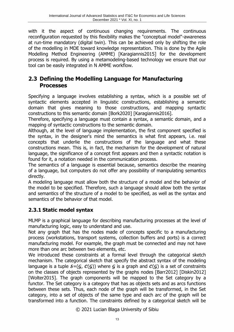
MLMP is a graphical language for describing manufacturing processes at the level of manufacturing logic, easy to understand and use. Not any graph that has the nodes made of concepts specific to a manufacturing process (workstations, transport systems, collection buffers and ports) is a correct manufacturing model. For example, the graph must be connected and may not have more than one arc between two elements, etc. We introduced these constraints at a formal level through the categorical sketch mechanism. The categorical sketch that specify the abstract syntax of the modeling language is a tuple 𝓢=(𝓖, 𝓒(𝓖)) where 𝓖 is a graph and 𝓒(𝓖) is a set of constraints

on the classes of objects represented by the graphs nodes [Barr2012] [Diskin2012] [Wolter2015]. The graph components will be mapped to the Set category by a functor. The Set category is a category that has as objects sets and as arcs functions between these sets. Thus, each node of the graph will be transformed, in the Set category, into a set of objects of the same type and each arc of the graph will be transformed into a function. The constraints defined by a categorical sketch will be

13



imposed on the corresponding sets of objects and functions in the Set category. Therefore, when defining the graph of a sketch and the corresponding constraints we must bear in mind that they will be mapped into the Set category. Therefore, in the graph of the sketch, each atomic concept, from the modeling domain, is represented by a node. The arcs of the sketch are called the sketch operators and allow the conditions to be imposed on the graph structure of the models. Categorical sketches are not designed as a notation, but as a mathematical structure that incorporates an exact formal syntax and semantics. A static visual model is the image of a sketch 𝓢=(𝓖,𝓒(𝓖)) through a functor in Set

category. Therefore, we have a class of models Mod(𝓢,Set) specified declaratively by

a categorical sketch 𝓢.

Figure 3 presents the categorical sketch for the MLMP constructed around the basic concepts (workstations xws, transport systems xts, collection buffers xbf and material ports xmp).

2.3.2 Behavioral syntax of MLMP

One of the key techniques in MDE for modeling the behavior of a system is the transformation of the model. This technique is also successfully used for the

Fig 3 Categorical sketch for the MLMP

14



automation of other model management operations, such as code generation, model optimization, translation from one DSML to another, simulation, etc. In the case of diagrammatic models, the transformation of the models is based on the transformation of graphs, which is a formal approach to structural changes of graphs by applying transformation rules [Plump2019] [Plump2010]. A graph rule, also called the production p=(L,R), is composed of two graphs; a left graph L, a right graph R and a mechanism that specifies the conditions and how to replace L with R. Although, in our case, the behavioral model is not based on structural transformations of the graph, but on changes of attribute values, we will use graph transformations because they provide the necessary context to locate the components involved in a transformation and to locate the critical regions that will be defined for parallel behavioral transformations. The double pushout (DPO) or single pushout (SPO) approaches are transformations in successive steps of the left graph to the right graph [Plump2010] [Plump2019] [Ehrig2015]. We will specify the behavior of the MLMP model, with DPO graph transformations. The transformation rules express local changes of the graphs and are therefore very suitable to describe the local transformations of the model states, on which the description of its behavior is based. A graph transformation rule is a formal concept that precisely defines the model's behavior through preconditions, postconditions and transformation steps ordered only by the causal dependence of the actions, which facilitates the application of independent rules in an arbitrary order. In the double-pushout (DPO) variant, a graphical production is denoted p=(L¬K®R) and contains three graphs: a left graph L, a right graph R and an interface graph K contained both in R, and in L, where the arrows represent two total monomorphisms pL:K®L and pR:K®R. In this variant, a production p contains besides graphs L and R and a bonding graph K, also two total graphical monomorphisms. The application of a production p=(L¬K®R) to a graph G begins with the localization of an occurrence of L in G, given by a total match monomorphism m: L®G. Then we must construct on a graph D by deleting from G the difference between L and K, that is D=G\(L\K). The final graph H is obtained by joining to D the difference between R and K, that is H=D+(R\K). In order for D=G\(L\K) to become a graph in which all edges have a source and target, a certain bonding condition must be fulfilled, which leads to a well-defined graph D.

2.3.3 Semantics of MLMP Language

As we have seen, in principle, a static visual model is the image of a sketch 𝓢=(𝓖,𝓒(𝓖)) through a functor. In order to also define the behavior of a model it is

necessary that the graph of the sketch be enriched besides the constraints (𝓖) also

with types, attributes and behavioral rules. An important extension of the graph 𝓖 is the introduction of a type of alphabet for

nodes and a type alphabet for arcs, and assignment of types to each element of it [Ehrig2015] [Campbell2018] [Campbell2019]. Thus, it becomes a type of graph. We will consider in the following that the name of each type is identified with the name of the corresponding element of the sketch. Then the typing of a model M: 𝓢®Set is made by a tuple MT=(M;typeM) where typeM

is a morphism from model M to the type graph 𝓖 thus defined typeM(X)=x where

15



XM(x) and x is a node or arc of the graph 𝓖 of the sketch. Thus, each element of a model will have a name and a type. We observe that the metamodel types can be similarly defined by a meta-metamodel. The states of a model will be defined by the values of some attributes associated with the nodes and edges of the graph of the structure of the model as well as the structure of the model. The evolution of the model is based on the modification of the structure of the model within the limits allowed by the constraints (𝓖) and on the

modification of the values of the attributes within the limits allowed by their type. An attributed graph is a graph extended by attaching attributes to the nodes and edges of a graph, so that the nodes and edges can also be characterized by the attribute values. These attributes are represented by edges that link the nodes and arcs of the sketch graph to the corresponding data domain [Campbell2019]. To be able to define the behavior of a model at the metamodel level, we will now introduce the notions of signing a behavioral rule and signing a system of behavioral rules. The signature of a behavioral rule is a tuple s=(LKR,CL,Act,CR) where: L, K and R are attributed graphs L,K,RGraph0, ls and rs are graph monomorphisms

ls,rsGraph1,

CL=(PL,arL) is a diagram predicate signature such that arL:PL®AGraph0, which we call

the precondition signature. CR=(PR,arR) is a diagram predicate signature such that arR:PR®AGraph0, which we call the postcondition signature. Act is an action signature that specifies how to transform the elements of graph L which is the domain of action into the components of graph R which composes the codomain of the action. Act has the shape graph arity a tuple ar=(arL,arR), where arL(Act)=L and arR(Act)=R. To simplify the exposure we will sometimes write an action in the form of Act(L;R). If we consider that the elements of graph L, the nodes and arcs, are (x1,...,xm) and the elements of graph R are (y1,...,ym) then (y1,...,ym):=Act(x1,...,xm) and therefore we will denote the graph L with L(x1,...,xm), the graph R with R(y1,...,ym), the graph K with K(z1,...,zl) and an action also with Act(x1,...,xm; y1,...,ym). Most of the times in applications Act is a set of operations wi:x1,...,xm®yi, i=1,…,m. The dynamic behavior of an MLMP model over time is accomplished by generic algorithms that implement the behavioral transformations. The simulation begins by initializing the system with data describing its initial state. The dynamics of the system are accomplished by the succession of the behavioral transformations executed. The semantics of an MLMP defines how process tokens are propagated through the arcs and objects of a model. In the modeling method concept the simulation of a model is based on mechanisms and algorithms that are written in a programming language. The behavior of the model is described by rules that specify how expressions are evaluated and commands executed. These rules provide an operational semantic that provides a language implementation.

16



2.4 Design (modelling) tool for the Factory of the Future

The modelling tool that implements the concept of modelling method, presented above, we called it the Digital Production Planner Tool (DPPT) and we implemented it on the ADOxx metamodeling platform. The tool should support the user to find a solution to a design problem. A design problem is formulated as an assortment of products characterized by the type of material and quantity that must be produced under some time and cost constraints. Because the most intuitive form of a model is the diagrammatic one, we chose to build a diagrammatic language.

2.4.1 The MLMP Language

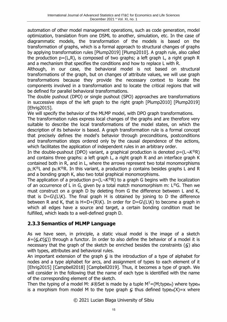
Diagrammatic models are, generally, graphs with certain constraints on their components, in which nodes and arcs are interpreted as a concept in the field of modelling [Wolter2015], [Karagiannis2016]. Designing a new visual DSML involves defining the syntax and semantics of the modelling domain. Defining the syntax of a DSML involves associating atomic concepts in the modelling domain with suggestive visual symbols and defining formal rules for composing these atomic concepts into complex concepts. Defining the semantics of modelling languages involves defining a semantic domain and mapping syntactic constructions to this semantic domain. Therefore, the syntax of a language is a way of expressing and manipulating semantics. The modelling language will have to provide mechanisms for specifying the static dimension of a model and the modelling instrument will have to include mechanisms and algorithms for simulating the behavioral dimension of the model. Both dimensions of a model, the static dimension and the behavioral dimension, are characterized by syntax and semantics. The atomic concepts in the specific domain of MLMP language modelling - corresponding to the nodes of the categorical sketch from Fig 2- are: Buffers, Workstations, Transport Machines and Ports. Figure 4 presents the metamodel implemented in ADOxx. The model results from

Fig. 4 The metamodel constructed from the categorical sketch

17



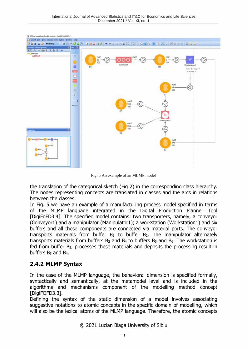
the translation of the categorical sketch (Fig 2) in the corresponding class hierarchy. The nodes representing concepts are translated in classes and the arcs in relations between the classes. In Fig. 5 we have an example of a manufacturing process model specified in terms of the MLMP language integrated in the Digital Production Planner Tool [DigiFoFD3.4]. The specified model contains: two transporters, namely, a conveyor (Conveyor1) and a manipulator (Manipulator1); a workstation (Workstation1) and six buffers and all these components are connected via material ports. The conveyor transports materials from buffer B1 to buffer B2. The manipulator alternately transports materials from buffers B3 and B4 to buffers B5 and B6. The workstation is fed from buffer B2, processes these materials and deposits the processing result in buffers B3 and B4.

2.4.2 MLMP Syntax

In the case of the MLMP language, the behavioral dimension is specified formally, syntactically and semantically, at the metamodel level and is included in the algorithms and mechanisms component of the modelling method concept [DigiFOFD3.3]. Defining the syntax of the static dimension of a model involves associating suggestive notations to atomic concepts in the specific domain of modelling, which will also be the lexical atoms of the MLMP language. Therefore, the atomic concepts

Fig. 5 An example of an MLMP model

18



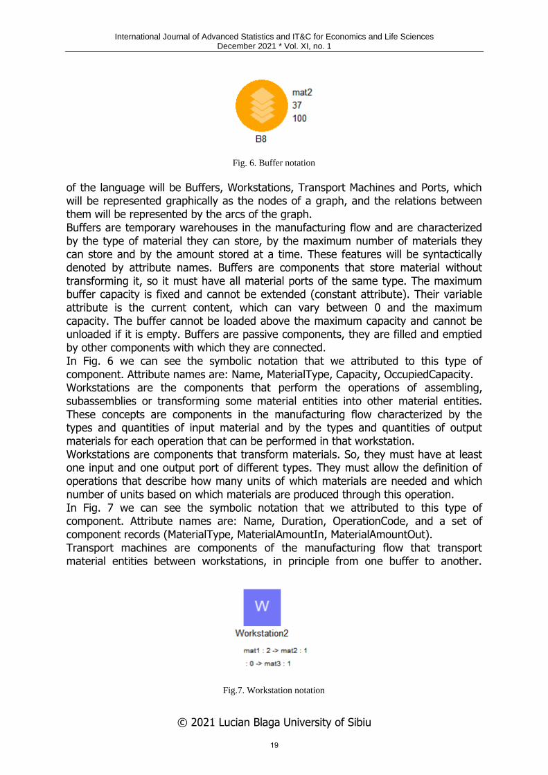
of the language will be Buffers, Workstations, Transport Machines and Ports, which will be represented graphically as the nodes of a graph, and the relations between them will be represented by the arcs of the graph. Buffers are temporary warehouses in the manufacturing flow and are characterized by the type of material they can store, by the maximum number of materials they can store and by the amount stored at a time. These features will be syntactically denoted by attribute names. Buffers are components that store material without transforming it, so it must have all material ports of the same type. The maximum buffer capacity is fixed and cannot be extended (constant attribute). Their variable attribute is the current content, which can vary between 0 and the maximum capacity. The buffer cannot be loaded above the maximum capacity and cannot be unloaded if it is empty. Buffers are passive components, they are filled and emptied by other components with which they are connected. In Fig. 6 we can see the symbolic notation that we attributed to this type of component. Attribute names are: Name, MaterialType, Capacity, OccupiedCapacity. Workstations are the components that perform the operations of assembling, subassemblies or transforming some material entities into other material entities. These concepts are components in the manufacturing flow characterized by the types and quantities of input material and by the types and quantities of output materials for each operation that can be performed in that workstation. Workstations are components that transform materials. So, they must have at least one input and one output port of different types. They must allow the definition of operations that describe how many units of which materials are needed and which number of units based on which materials are produced through this operation. In Fig. 7 we can see the symbolic notation that we attributed to this type of component. Attribute names are: Name, Duration, OperationCode, and a set of component records (MaterialType, MaterialAmountIn, MaterialAmountOut). Transport machines are components of the manufacturing flow that transport material entities between workstations, in principle from one buffer to another.

Fig.7. Workstation notation

Fig. 6. Buffer notation

19



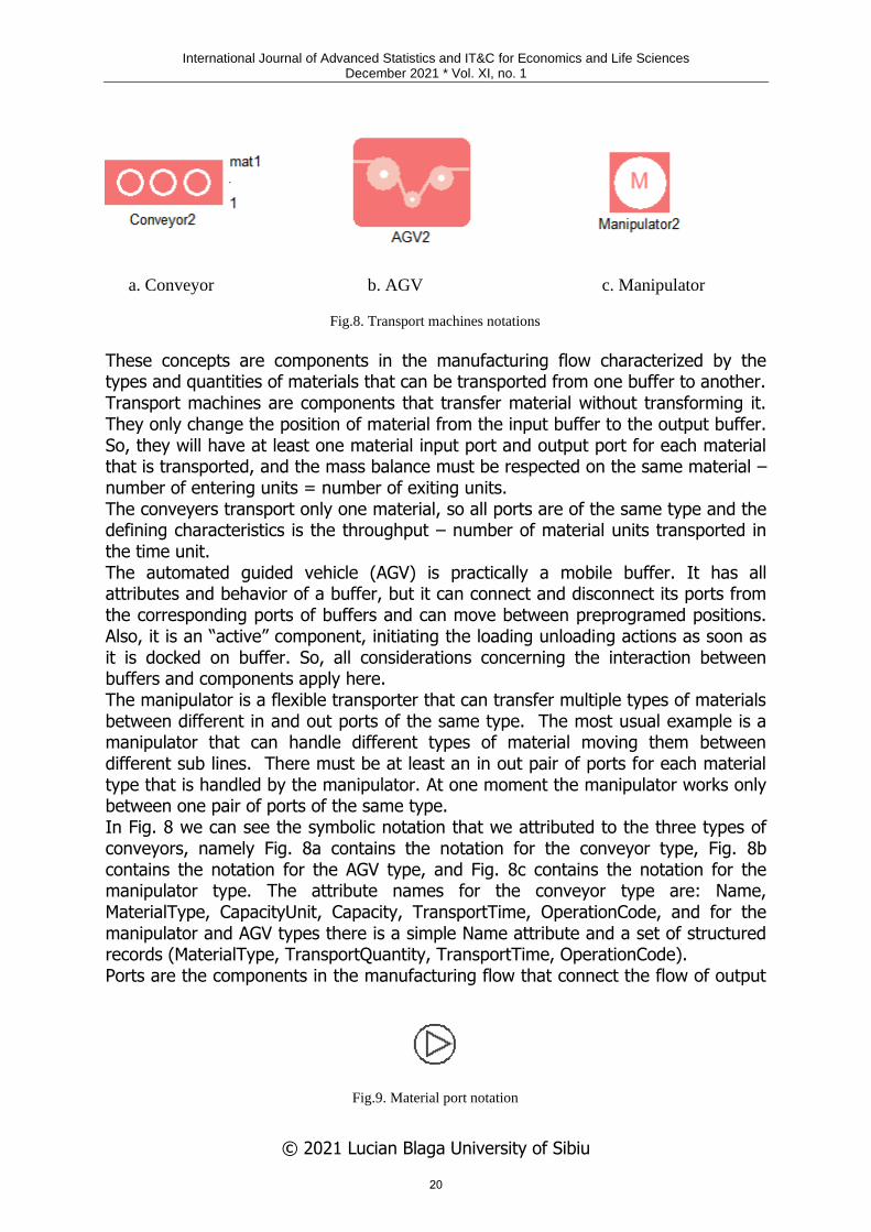
These concepts are components in the manufacturing flow characterized by the types and quantities of materials that can be transported from one buffer to another. Transport machines are components that transfer material without transforming it. They only change the position of material from the input buffer to the output buffer. So, they will have at least one material input port and output port for each material that is transported, and the mass balance must be respected on the same material – number of entering units = number of exiting units. The conveyers transport only one material, so all ports are of the same type and the defining characteristics is the throughput – number of material units transported in the time unit. The automated guided vehicle (AGV) is practically a mobile buffer. It has all attributes and behavior of a buffer, but it can connect and disconnect its ports from the corresponding ports of buffers and can move between preprogramed positions. Also, it is an “active” component, initiating the loading unloading actions as soon as it is docked on buffer. So, all considerations concerning the interaction between buffers and components apply here. The manipulator is a flexible transporter that can transfer multiple types of materials between different in and out ports of the same type. The most usual example is a manipulator that can handle different types of material moving them between different sub lines. There must be at least an in out pair of ports for each material type that is handled by the manipulator. At one moment the manipulator works only between one pair of ports of the same type. In Fig. 8 we can see the symbolic notation that we attributed to the three types of conveyors, namely Fig. 8a contains the notation for the conveyor type, Fig. 8b contains the notation for the AGV type, and Fig. 8c contains the notation for the manipulator type. The attribute names for the conveyor type are: Name, MaterialType, CapacityUnit, Capacity, TransportTime, OperationCode, and for the manipulator and AGV types there is a simple Name attribute and a set of structured records (MaterialType, TransportQuantity, TransportTime, OperationCode). Ports are the components in the manufacturing flow that connect the flow of output

a. Conveyor b. AGV c. Manipulator

Fig.8. Transport machines notations

Fig.9. Material port notation

20



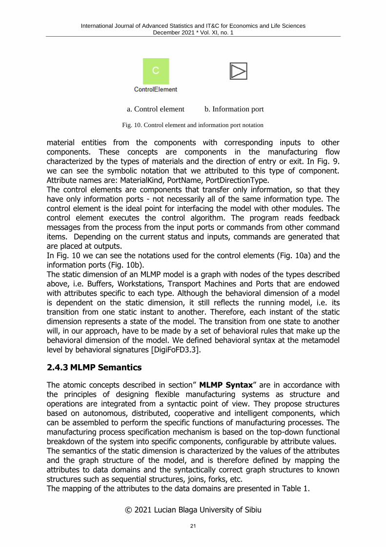
material entities from the components with corresponding inputs to other components. These concepts are components in the manufacturing flow characterized by the types of materials and the direction of entry or exit. In Fig. 9. we can see the symbolic notation that we attributed to this type of component. Attribute names are: MaterialKind, PortName, PortDirectionType. The control elements are components that transfer only information, so that they have only information ports - not necessarily all of the same information type. The control element is the ideal point for interfacing the model with other modules. The control element executes the control algorithm. The program reads feedback messages from the process from the input ports or commands from other command items. Depending on the current status and inputs, commands are generated that are placed at outputs. In Fig. 10 we can see the notations used for the control elements (Fig. 10a) and the information ports (Fig. 10b). The static dimension of an MLMP model is a graph with nodes of the types described above, i.e. Buffers, Workstations, Transport Machines and Ports that are endowed with attributes specific to each type. Although the behavioral dimension of a model is dependent on the static dimension, it still reflects the running model, i.e. its transition from one static instant to another. Therefore, each instant of the static dimension represents a state of the model. The transition from one state to another will, in our approach, have to be made by a set of behavioral rules that make up the behavioral dimension of the model. We defined behavioral syntax at the metamodel level by behavioral signatures [DigiFoFD3.3].

2.4.3 MLMP Semantics

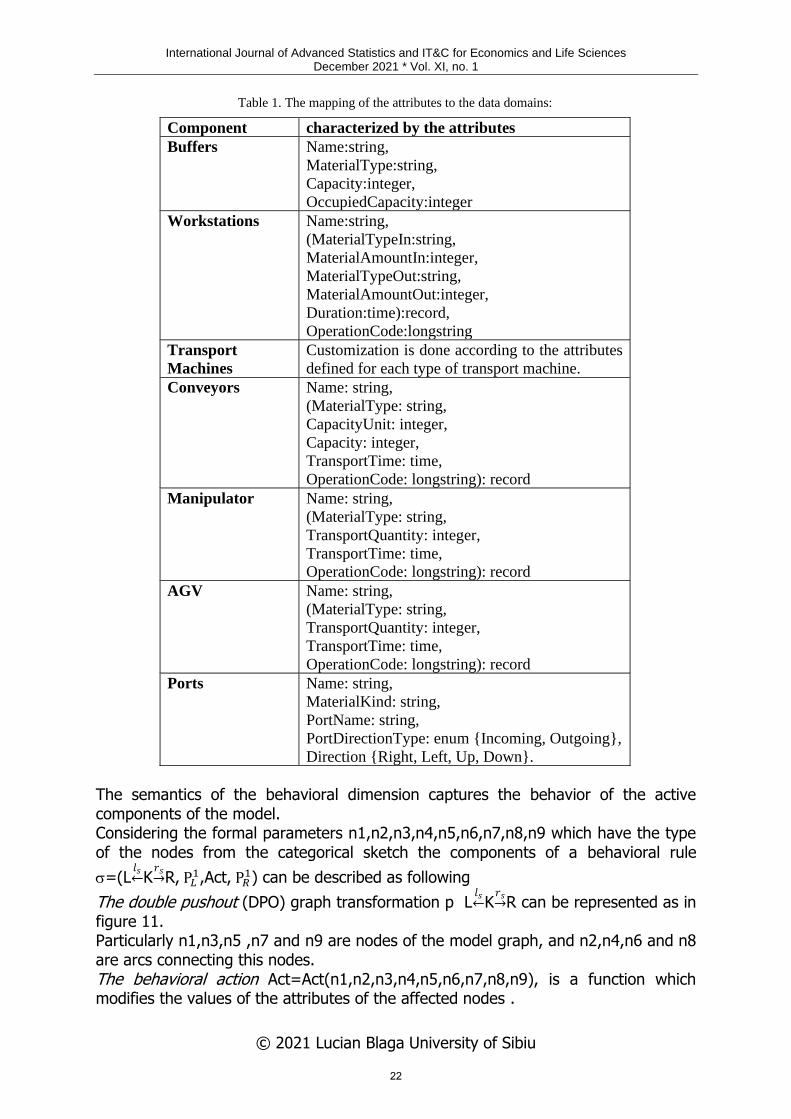
The atomic concepts described in section” MLMP Syntax” are in accordance with the principles of designing flexible manufacturing systems as structure and operations are integrated from a syntactic point of view. They propose structures based on autonomous, distributed, cooperative and intelligent components, which can be assembled to perform the specific functions of manufacturing processes. The manufacturing process specification mechanism is based on the top-down functional breakdown of the system into specific components, configurable by attribute values. The semantics of the static dimension is characterized by the values of the attributes and the graph structure of the model, and is therefore defined by mapping the attributes to data domains and the syntactically correct graph structures to known structures such as sequential structures, joins, forks, etc. The mapping of the attributes to the data domains are presented in Table 1.

a. Control element b. Information port

Fig. 10. Control element and information port notation

21



The semantics of the behavioral dimension captures the behavior of the active components of the model. Considering the formal parameters n1,n2,n3,n4,n5,n6,n7,n8,n9 which have the type of the nodes from the categorical sketch the components of a behavioral rule

=(L𝑙𝑠←K

𝑟𝑠→R, P𝐿

1,Act, P𝑅1) can be described as following

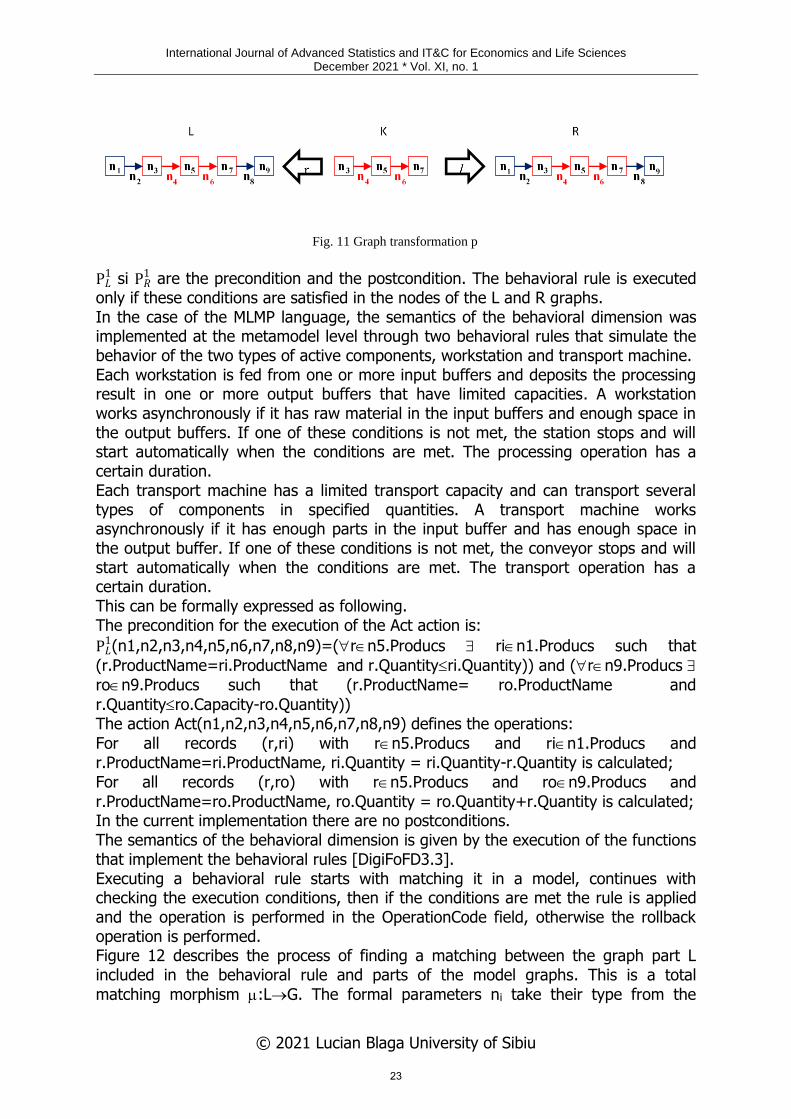
The double pushout (DPO) graph transformation p L𝑙𝑠←K

𝑟𝑠→R can be represented as in

figure 11. Particularly n1,n3,n5 ,n7 and n9 are nodes of the model graph, and n2,n4,n6 and n8 are arcs connecting this nodes. The behavioral action Act=Act(n1,n2,n3,n4,n5,n6,n7,n8,n9), is a function which modifies the values of the attributes of the affected nodes .

Table 1. The mapping of the attributes to the data domains:

Component characterized by the attributes

Buffers Name:string,

MaterialType:string,

Capacity:integer,

OccupiedCapacity:integer

Workstations Name:string,

(MaterialTypeIn:string,

MaterialAmountIn:integer,

MaterialTypeOut:string,

MaterialAmountOut:integer,

Duration:time):record,

OperationCode:longstring

Transport

Machines

Customization is done according to the attributes

defined for each type of transport machine.

Conveyors Name: string,

(MaterialType: string,

CapacityUnit: integer,

Capacity: integer,

TransportTime: time,

OperationCode: longstring): record

Manipulator Name: string,


TransportQuantity: integer,



AGV Name: string,


TransportQuantity: integer,



Ports Name: string,

MaterialKind: string,

PortName: string,

PortDirectionType: enum {Incoming, Outgoing},

Direction {Right, Left, Up, Down}.

22



P𝐿1 si P𝑅

1 are the precondition and the postcondition. The behavioral rule is executed only if these conditions are satisfied in the nodes of the L and R graphs. In the case of the MLMP language, the semantics of the behavioral dimension was implemented at the metamodel level through two behavioral rules that simulate the behavior of the two types of active components, workstation and transport machine. Each workstation is fed from one or more input buffers and deposits the processing result in one or more output buffers that have limited capacities. A workstation works asynchronously if it has raw material in the input buffers and enough space in the output buffers. If one of these conditions is not met, the station stops and will start automatically when the conditions are met. The processing operation has a certain duration. Each transport machine has a limited transport capacity and can transport several types of components in specified quantities. A transport machine works asynchronously if it has enough parts in the input buffer and has enough space in the output buffer. If one of these conditions is not met, the conveyor stops and will start automatically when the conditions are met. The transport operation has a certain duration. This can be formally expressed as following. The precondition for the execution of the Act action is:

P𝐿1(n1,n2,n3,n4,n5,n6,n7,n8,n9)=(rn5.Producs rin1.Producs such that

(r.ProductName=ri.ProductName and r.Quantityri.Quantity)) and (rn9.Producs

ron9.Producs such that (r.ProductName= ro.ProductName and

r.Quantityro.Capacity-ro.Quantity)) The action Act(n1,n2,n3,n4,n5,n6,n7,n8,n9) defines the operations:

For all records (r,ri) with rn5.Producs and rin1.Producs and r.ProductName=ri.ProductName, ri.Quantity = ri.Quantity-r.Quantity is calculated;

For all records (r,ro) with rn5.Producs and ron9.Producs and

r.ProductName=ro.ProductName, ro.Quantity = ro.Quantity+r.Quantity is calculated; In the current implementation there are no postconditions. The semantics of the behavioral dimension is given by the execution of the functions that implement the behavioral rules [DigiFoFD3.3]. Executing a behavioral rule starts with matching it in a model, continues with checking the execution conditions, then if the conditions are met the rule is applied and the operation is performed in the OperationCode field, otherwise the rollback operation is performed. Figure 12 describes the process of finding a matching between the graph part L included in the behavioral rule and parts of the model graphs. This is a total

matching morphism :L→G. The formal parameters ni take their type from the

Fig. 11 Graph transformation p

23



sketch S. The model is an image of the sketch 𝓢 through the functor 𝕴. In the

example the matched fragment is a part of a model representing a manufacturing system. The n1to n9 chain matches a line composed of the buffers B1 and B2 and of the workstation WS1. WS1 is feed from B1 through the port P1 and stores is output in B2 through the P2 port. The current values of the attributes of the matched nodes (e.g. Material Type and Occupied Capacity of B1) are replaced in the precondition predicates of the behavioral rule. If the predicates hold the function corresponding to the behavioral action Act is applied on the attributes values and they are updated correspondingly. The dynamic behavior of an MLMP model over time is accomplished by generic algorithms that implement the behavioral transformations. The simulation begins by initializing the system with data describing its initial state. The dynamics of the system are accomplished by the succession of the behavioral transformations executed. The semantics of an MLMP defines how process tokens are propagated through the arcs and objects of a model. In the modelling method concept the simulation of a model is based on mechanisms and algorithms that are written in a programming language. The behavior of the model is described by rules that specify how expressions are evaluated and commands executed. These rules provide an operational semantic that provides a language implementation. Preconditions and postconditions are implemented as logical expressions in ADOScript. The behavioral actions are implemented as

Fig. 12 The match µ of the shape graph to the model M

24



ADOScript scripts.

2.5 Example of the chocolate production line

In this section a solution to the design problem is illustrated (Fig.13). The position and dimension have high relevance for the capabilities of the design solution. The actual version only supports for the relative positioning and orientation of components. Further support will be added with next versions.

• AGV1 transports the buckets with chocolate ganache mass (m1) from the buffer B1 to the buffer B3;

• AGV2 transports the cardboard packaging material (m2) from the buffer B2 to the buffer B7;

• On line 1 (L1), the chocolate ganache mass (m1) is taken from B3 by the workstation WS1 which outputs the chocolate truffles (m3). The product m3 is discharged in the buffer B4 feeding the transport line with freezing areas B11. The chocolate truffles are loaded in the buffer B5, which is feeding WS2. WS2 forms the aluminum bags from the aluminium (m7) stored in the roll (buffer B12) and fills them with chocolate truffles. The product is m4 – aluminum bags filled with chocolate truffles – and is stored in the buffer B6;

• On line 2 (L2), cardboard packaging material (m2) is loaded from the buffer B7 to the WS3, where the cardboard packaging boxes (m5) are formed; they are loaded in the buffer B8;

• On the assembly line, the Manipulator M1 transfers m4, from the buffer B6 in the buffer B9 and m5, from the buffer B8 to the buffer B10. The buffers are

Fig. 13 The MLMP model of the chocolate truffles manufacturing line

25



feeding the packaging machine WS4, that stores the final products m6 (cardboard boxes having aluminum bags with truffles) in B11 buffer.

2.5.1 Simulating and analyzing the model

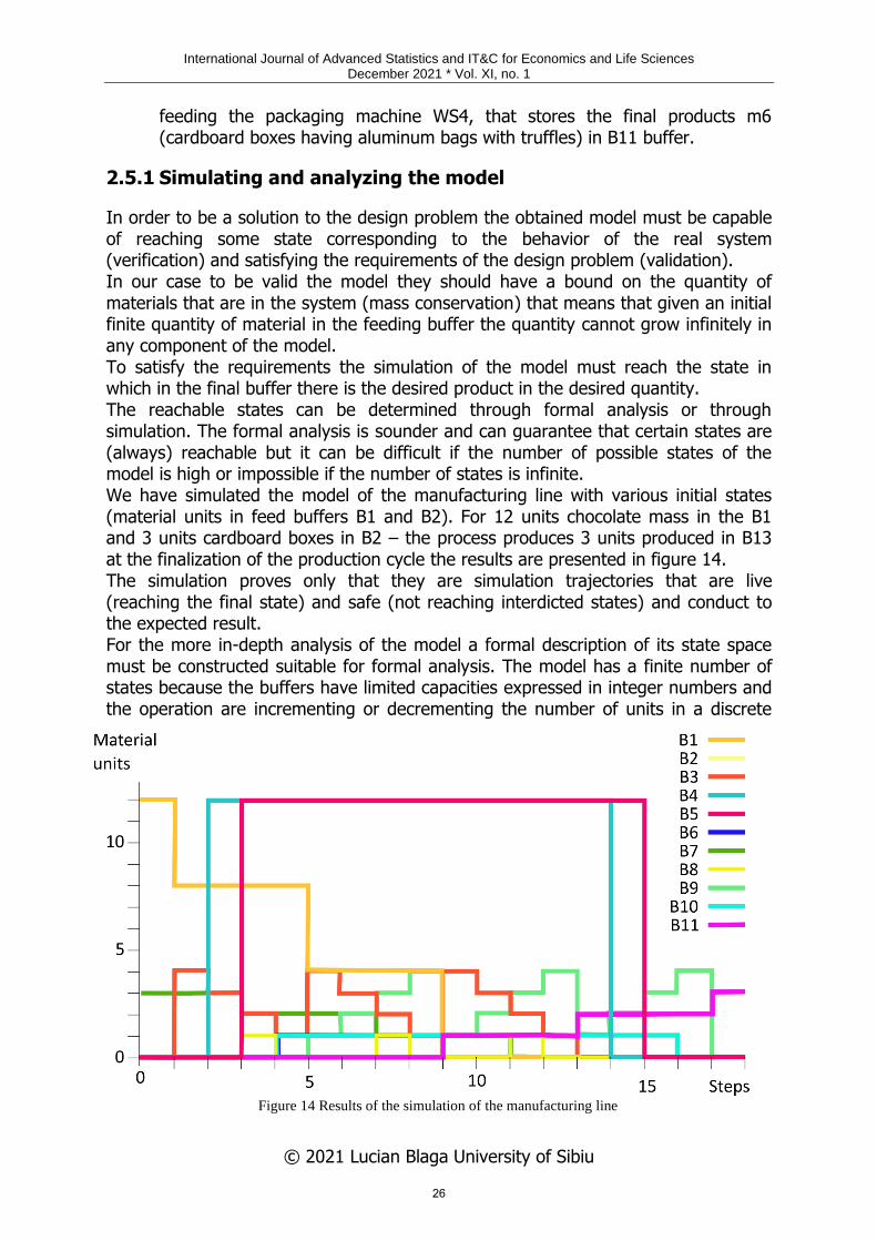
In order to be a solution to the design problem the obtained model must be capable of reaching some state corresponding to the behavior of the real system (verification) and satisfying the requirements of the design problem (validation). In our case to be valid the model they should have a bound on the quantity of materials that are in the system (mass conservation) that means that given an initial finite quantity of material in the feeding buffer the quantity cannot grow infinitely in any component of the model. To satisfy the requirements the simulation of the model must reach the state in which in the final buffer there is the desired product in the desired quantity. The reachable states can be determined through formal analysis or through simulation. The formal analysis is sounder and can guarantee that certain states are (always) reachable but it can be difficult if the number of possible states of the model is high or impossible if the number of states is infinite. We have simulated the model of the manufacturing line with various initial states (material units in feed buffers B1 and B2). For 12 units chocolate mass in the B1 and 3 units cardboard boxes in B2 – the process produces 3 units produced in B13 at the finalization of the production cycle the results are presented in figure 14. The simulation proves only that they are simulation trajectories that are live (reaching the final state) and safe (not reaching interdicted states) and conduct to the expected result. For the more in-depth analysis of the model a formal description of its state space must be constructed suitable for formal analysis. The model has a finite number of states because the buffers have limited capacities expressed in integer numbers and the operation are incrementing or decrementing the number of units in a discrete

Figure 14 Results of the simulation of the manufacturing line

26



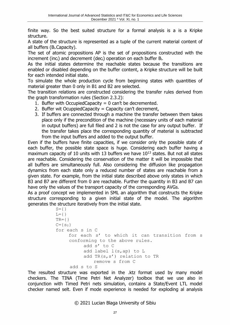
finite way. So the best suited structure for a formal analysis is a is a Kripke structure. A state of the structure is represented as a tuple of the current material content of all buffers (Bi.Capacity). The set of atomic propositions AP is the set of propositions constructed with the increment (inci) and decrement (deci) operation on each buffer Bi. As the initial states determine the reachable states because the transitions are enabled or disabled depending on the buffer content, a Kripke structure will be built for each intended initial state. To simulate the whole production cycle from beginning states with quantities of material greater than 0 only in B1 and B2 are selected. The transition relations are constructed considering the transfer rules derived from the graph transformation rules (Section 2.3.2):

1. Buffer with OccupiedCapacity = 0 can’t be decremented. 2. Buffer wit OcuppiedCapacity = Capacity can’t decrement, 3. If buffers are connected through a machine the transfer between them takes

place only if the precondition of the machine (necessary units of each material in output buffers) are full filed and 2 is not the case for any output buffer. If the transfer takes place the corresponding quantity of material is subtracted from the input buffers and added to the output buffer.

Even if the buffers have finite capacities, if we consider only the possible state of each buffer, the possible state space is huge. Considering each buffer having a maximum capacity of 10 units with 13 buffers we have 1013 states. But not all states are reachable. Considering the conservation of the matter it will be impossible that all buffers are simultaneously full. Also considering the diffusion like propagation dynamics from each state only a reduced number of states are reachable from a given state. For example, from the initial state described above only states in which B3 and B7 are different from 0 are reachable. Further the quantity in B3 and B7 can have only the values of the transport capacity of the corresponding AVGs. As a proof concept we implemented in SML an algorithm that constructs the Kripke structure corresponding to a given initial state of the model. The algorithm generates the structure iteratively from the initial state.

S={}

L={}

TR={}

C={s0}

for each s in C

for each s’ to which it can transition from s

conforming to the above rules.

add s’ to C

add label l(s,ap) to L

add TR(s,s’) relation to TR

remove s from C

add s to S

The resulted structure was exported in the .ktz format used by many model checkers. The TINA (Time Petri Net Analyzer) toolbox that we use also in conjunction with Timed Petri nets simulation, contains a State/Event LTL model checker named selt. Even if mode experience is needed for exploding al analysis

27



capacity of the tool we succeeded in expressing some properties and testing them for Kripke structures constructed with different initial states. So the proposition F(B13=3) that express the fact that eventually (Finally) the end material buffer will contain 3 material units was proven true for the Kripke structure constructed from the same initial state as the simulation(B1=12,B2=3). This proves that the system will arrive to the desired final state.

2.6 Extending the analysis capabilities

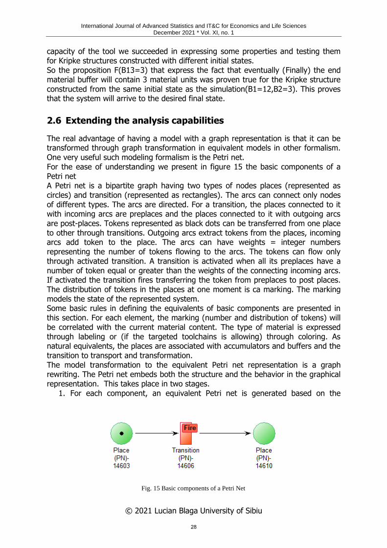
The real advantage of having a model with a graph representation is that it can be transformed through graph transformation in equivalent models in other formalism. One very useful such modeling formalism is the Petri net. For the ease of understanding we present in figure 15 the basic components of a Petri net A Petri net is a bipartite graph having two types of nodes places (represented as circles) and transition (represented as rectangles). The arcs can connect only nodes of different types. The arcs are directed. For a transition, the places connected to it with incoming arcs are preplaces and the places connected to it with outgoing arcs are post-places. Tokens represented as black dots can be transferred from one place to other through transitions. Outgoing arcs extract tokens from the places, incoming arcs add token to the place. The arcs can have weights = integer numbers representing the number of tokens flowing to the arcs. The tokens can flow only through activated transition. A transition is activated when all its preplaces have a number of token equal or greater than the weights of the connecting incoming arcs. If activated the transition fires transferring the token from preplaces to post places. The distribution of tokens in the places at one moment is ca marking. The marking models the state of the represented system. Some basic rules in defining the equivalents of basic components are presented in this section. For each element, the marking (number and distribution of tokens) will be correlated with the current material content. The type of material is expressed through labeling or (if the targeted toolchains is allowing) through coloring. As natural equivalents, the places are associated with accumulators and buffers and the transition to transport and transformation. The model transformation to the equivalent Petri net representation is a graph rewriting. The Petri net embeds both the structure and the behavior in the graphical representation. This takes place in two stages.

1. For each component, an equivalent Petri net is generated based on the

Fig. 15 Basic components of a Petri Net

28



corresponding behavioral rule =(L𝑙𝑠←K

𝑟𝑠→R, P𝐿

1,Act, P𝑅1) by following this rule

• Each material content attribute is represented by a place. The current number of tokens in the place (the current marking) represents the current value of this attribute.

• The Act is implemented through the connections In the Petri net. Considering that:

o Each transition subtracts from the preplaces the number of tokens specified as label on the connecting incoming arc.

o Each transitions ads to the post places the number of tokens specified as label on the connecting outgoing arc.

the graph representation of the mathematical expression of the action is transformed in a Petri net. The net connects to the places representing the attributes but can include supplementary places.

• The preconditions and post conditions are implemented using the implicit firing rule of the Petri net. According to this rule the transition is not firing if the marking of each preplace is lesser then the label of the connecting incoming arc. So each transition must be connected to al places that represent attributes that condition its activation.

• The Petri net of the components includes also the corresponding ports from the in MLMP models. They are translated to input places - places with only outgoing arcs and output places - places with only ingoing arcs.

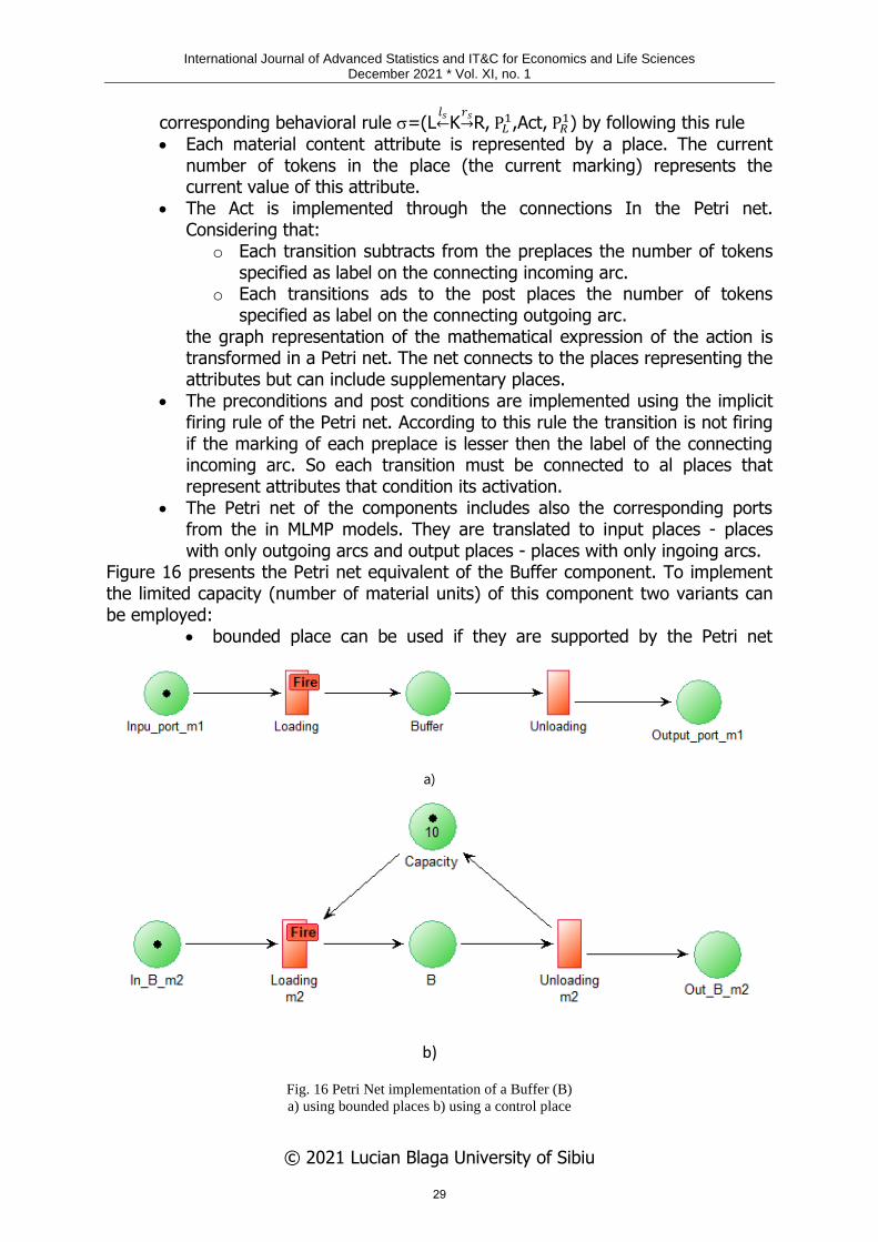
Figure 16 presents the Petri net equivalent of the Buffer component. To implement the limited capacity (number of material units) of this component two variants can be employed:

• bounded place can be used if they are supported by the Petri net

a)

b)

Fig. 16 Petri Net implementation of a Buffer (B)

a) using bounded places b) using a control place

29



modeling, simulation and analysis toolchain (e.g. BeeUp) (fig.16a) • a supplementary control place (as employed in the Petri net-based

control theory) is provided with an initial marking corresponding to this capacity. (Fig 16b))

Figure 17 presents the Petri net model corresponding to a component from the Conveyor, Belt and Pipe subclass of the transportation machines class. The Capacity of the transport line is implemented in the arc weight. In the presented example 2 units of the transported material are transferred from the input port In_t_m3 to the output port Out_m3 in each step which corresponds to the TransportTime. The presence of the command place C allows the control of the transport – blocking the

Fig. 18 Petri Net implementation of a Manipulator

Fig. 17 Petri Net implementation of a transport component (Conveyor,Belt,Pipe)

30



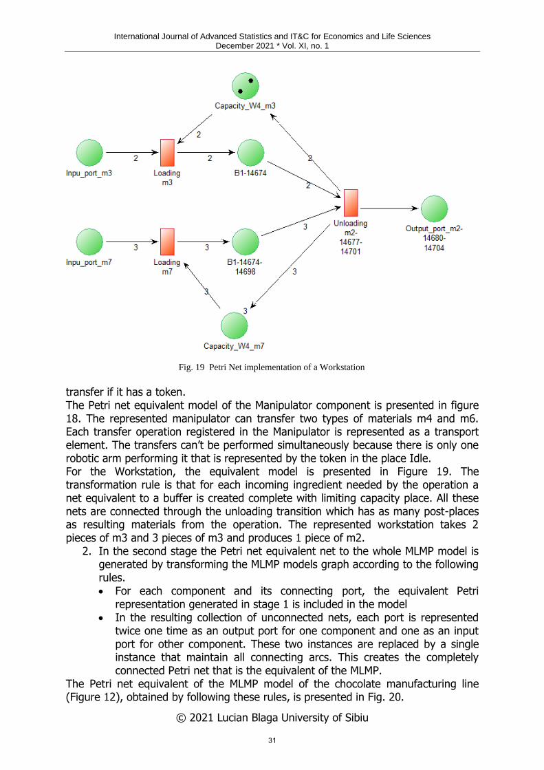
transfer if it has a token. The Petri net equivalent model of the Manipulator component is presented in figure 18. The represented manipulator can transfer two types of materials m4 and m6. Each transfer operation registered in the Manipulator is represented as a transport element. The transfers can’t be performed simultaneously because there is only one robotic arm performing it that is represented by the token in the place Idle. For the Workstation, the equivalent model is presented in Figure 19. The transformation rule is that for each incoming ingredient needed by the operation a net equivalent to a buffer is created complete with limiting capacity place. All these nets are connected through the unloading transition which has as many post-places as resulting materials from the operation. The represented workstation takes 2 pieces of m3 and 3 pieces of m3 and produces 1 piece of m2.

2. In the second stage the Petri net equivalent net to the whole MLMP model is generated by transforming the MLMP models graph according to the following rules. • For each component and its connecting port, the equivalent Petri

representation generated in stage 1 is included in the model • In the resulting collection of unconnected nets, each port is represented

twice one time as an output port for one component and one as an input port for other component. These two instances are replaced by a single instance that maintain all connecting arcs. This creates the completely connected Petri net that is the equivalent of the MLMP.

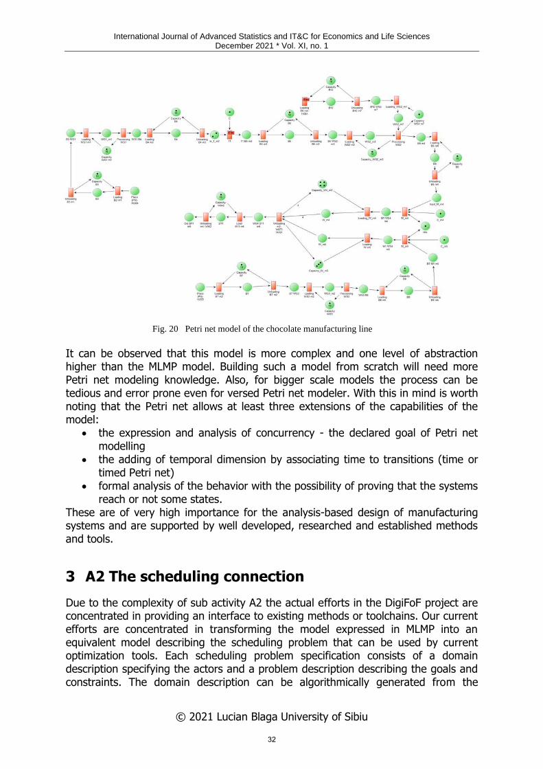
The Petri net equivalent of the MLMP model of the chocolate manufacturing line (Figure 12), obtained by following these rules, is presented in Fig. 20.

Fig. 19 Petri Net implementation of a Workstation

31



It can be observed that this model is more complex and one level of abstraction higher than the MLMP model. Building such a model from scratch will need more Petri net modeling knowledge. Also, for bigger scale models the process can be tedious and error prone even for versed Petri net modeler. With this in mind is worth noting that the Petri net allows at least three extensions of the capabilities of the model:

• the expression and analysis of concurrency - the declared goal of Petri net modelling

• the adding of temporal dimension by associating time to transitions (time or timed Petri net)

• formal analysis of the behavior with the possibility of proving that the systems reach or not some states.

These are of very high importance for the analysis-based design of manufacturing systems and are supported by well developed, researched and established methods and tools.

3 A2 The scheduling connection

Due to the complexity of sub activity A2 the actual efforts in the DigiFoF project are concentrated in providing an interface to existing methods or toolchains. Our current efforts are concentrated in transforming the model expressed in MLMP into an equivalent model describing the scheduling problem that can be used by current optimization tools. Each scheduling problem specification consists of a domain description specifying the actors and a problem description describing the goals and constraints. The domain description can be algorithmically generated from the

Fig. 20 Petri net model of the chocolate manufacturing line

32



manufacturing line model in MLMP. The problem description is a more individual and a particular task for the designer. We are working currently to provide the possibility for the designer to use:

● the classic approach to transform the case in a matrix representation suitable for a mathematical optimization tool (e.g R , Matlab)

● solution search through direct simulation in the DPPT tool or in a Petri net simulator after transformation. This can be extended to a heuristic design space exploration using gradient search for finding the optimum.

● the transformation to a version/variant of the Planning Domain Definition Language (PDDL). Having this PDDL description of the scheduling problem a variety of planner that accept this format can be used to generate an optimized schedule

4 A3 The automation path

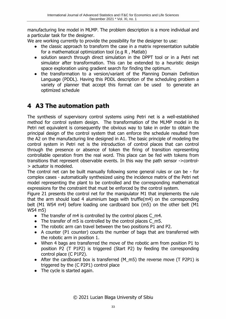
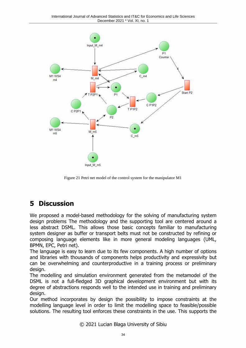
The synthesis of supervisory control systems using Petri net is a well-established method for control system design. The transformation of the MLMP model in its Petri net equivalent is consequently the obvious way to take in order to obtain the principal design of the control system that can enforce the schedule resulted from the A2 on the manufacturing line designed in A1. The basic principle of modeling the control system in Petri net is the introduction of control places that can control through the presence or absence of token the firing of transition representing controllable operation from the real word. This place can be fed with tokens from transitions that represent observable events. In this way the path sensor ->control-> actuator is modeled. The control net can be built manually following some general rules or can be - for complex cases - automatically synthesized using the incidence matrix of the Petri net model representing the plant to be controlled and the corresponding mathematical expressions for the constraint that must be enforced by the control system. Figure 21 presents the control net for the manipulator M1 that implements the rule that the arm should load 4 aluminium bags with truffle(m4) on the corresponding belt (M1 WS4 m4) before loading one cardboard box (m5) on the other belt (M1 WS4 m5)

● The transfer of m4 is controlled by the control places C_m4. ● The transfer of m5 is controlled by the control places C_m5. ● The robotic arm can travel between the two positions P1 and P2. ● A counter (P1 counter) counts the number of bags that are transferred with

the robotic arm in position 1. ● When 4 bags are transferred the move of the robotic arm from position P1 to

position P2 (T P1P2) is triggered (Start P2) by feeding the corresponding control place (C P1P2).

● After the cardboard box is transferred (M_m5) the reverse move (T P2P1) is triggered by the (C P2P1) control place

● The cycle is started again.

33



5 Discussion

We proposed a model-based methodology for the solving of manufacturing system design problems The methodology and the supporting tool are centered around a less abstract DSML. This allows those basic concepts familiar to manufacturing system designer as buffer or transport belts must not be constructed by refining or composing language elements like in more general modeling languages (UML, BPMN, EPC, Petri net). The language is easy to learn due to its few components. A high number of options and libraries with thousands of components helps productivity and expressivity but can be overwhelming and counterproductive in a training process or preliminary design. The modelling and simulation environment generated from the metamodel of the DSML is not a full-fledged 3D graphical development environment but with its degree of abstractions responds well to the intended use in training and preliminary design. Our method incorporates by design the possibility to impose constraints at the modelling language level in order to limit the modelling space to feasible/possible solutions. The resulting tool enforces these constraints in the use. This supports the

Figure 21 Petri net model of the control system for the manipulator M1

34



development of feasible designs even by inexperienced designers and reduces the costs by avoiding incorrect models. The out-of-the-box extensibility of the DPPT is mostly quantitatively – the common user can add variation of the same type of component but cannot easily define an entirely new type of component. But the access to the conceptual model allows the translation of the model to other modelling language. The basic functionality for this is already implemented in the form of XML import export. By translating to more expressive and supported languages like Petri net or PDDL the functionality can be greatly enhanced covering all activities proposed for the design method. This can give an advantage over the majority of tools that from intellectual property and commercial reasons have a limited interoperability with other modelling and simulation tools. Because it is integrated in the ADOxx ecosystem, DPPT can access all facilities that this development environment offers as the combination of different modeling languages similar, shared repositories use of Web services, interface with CyberPhysical Systems and integrations in an Agile Modelling Method Engineering workflow.

6 Conclusion and Future Development

This whitepaper demonstrates the feasibility of the theoretical concepts presented in [DigiFoFD3.3] and provides motivational arguments for the implementation of DSMLs as basic components of the modelling method concept. The concepts that represent the lexical atoms of language and the relationships between them determine the design principles of flexible manufacturing systems as structure, components, and operations. The flexible manufacturing cell model becomes in this context a structure based on autonomous, distributed, cooperative and intelligent modules, able to fulfil the specific functions of the manufacturing process. An important aspect of manufacturing process models is building complex functions from a given set of simple functions, using different operations on functions such as composition and repeat composition. Category theory is exactly the right algebra for such constructions. The theory of categories works with patterns or forms in which each of these forms describe different aspects of the real world. Category theory offers both a language, and a lot of conceptual tools to efficiently handle models. Although the developed DPPT is only an initial version with a minimal set of facilities, it highlights the advantages of such a diagrammatic DSML. A DSML, with a small set of well-chosen domain concepts, can have complex semantics to cover the modelling domain. This is because the behavioral dimension of the models is embedded at the metamodel level. Also, this semantic load is due to the unlimited complexity of the relations between the lexical atoms of a diagrammatic language in contrast to the limited relations between the lexical atoms of the textual languages. We could say that the transition from programming languages to domain-specific diagrammatic modelling languages is as important as the transition from programming in assembly languages to programming in high-level languages. As we can see such a language is also intuitive and easily accessible due to its visual character especially if the notations used for atomic components are well chosen.

35



These features of a domain-specific diagrammatic modelling language make it usable in all domain-specific modelling phases since it is accessible to all parties involved in the modelling process. The DPP design method and tool developed is easy to learn and to use in the context of no or little design experience. It can be downloaded from the link http://digifof.omilab.ulbsibiu.ro/psm/content/dppt/info. Using the OMiLAB ecosystem,

the tool facilitates the collaboration between the training team members and allows the establishment of collaborative networks on the knowledge triangle [Karagiannis2020].

Acknowledgment This work was supported from the European Union’s EACEA Erasmus+ Programme Key Action 2 - Knowledge Alliances under the Grant Agreement Number 2018-2533 / 001-001, Project Nr. 601089-EPP-1-2018-1-RO-EPPKA2-KA, the project THE FOF-DESIGNER: DIGITAL DESIGN SKILLS FOR FACTORIES OF THE FUTURE, (acronine DigiFoF).

7 References

[Barr2012] Michael Barr And Charles Wells, Category Theory For Computing Science- Reprints in

Theory and Applications of Categories, No. 22, 2012. [Bork2019] D. Bork, R.A. Buchman, D. Karagiannis, M. Lee, E.T. Miron, An Open Platform for

Modeling Method Conceptualization: The OMiLAB Digital Ecosystem, Communications of the Association for Information Systems, forthcoming, http://eprints.cs.univie.ac.at/5462/1/CAIS-

OMiLAB-final-withFront.pdf (2019)

[Bork2020] Dominik Bork, Dimitris Karagiannis, Benedikt Pittl, A survey of modeling language specification techniques, Information Systems 87 (2020) 101425, journal homepage:

www.elsevier.com/locate/is [Campbell2018] G. Campbell, ‘Algebraic graph transformation: A crash course’, Department of

Computer Science, University of York, UK, Tech. Rep., 2018. [Online]. Available:

https://cdn.gjcampbell.co.uk/2018/Graph-Transformation.pdf. [Campbell2019] G. Campbell, B. Courtehoute and D. Plump, ‘Linear-time graph algorithms in GP2’,

Department of Computer Science, University of York, UK, Submitted for publication, 2019. [Online]. Available: https://cdn.gjcampbell.co.uk/2019/Linear-Time-GP2-Preprint.pdf.

[Craciunean2018] D.C. Crăciunean, D. Karagiannis, Categorical Modeling Method of Intelligent WorkFlow. In: Groza A., Prasath R. (eds) Mining Intelligence and Knowledge Exploration.

MIKE Lecture Notes in Computer Science, vol 11308. Springer, Cham (2018).

[Craciunean2019]D.C. Crăciunean, Categorical Grammars for Processes Modeling, International Journal of Advanced Computer Science and Applications(IJACSA), 10(1), (2019)

[DigiFoF2019] Report on needs and demands for FoF-design: Findings and recommendations, DigiFoF Project Nr.601089-EPP-1-2018-1-RO-EPPKA2-KA, 30.06.2019,

https://digifof.eu/sites/default/files/casestudiesfiles/d1.2_report_on_needs_and_demands_for

_fof-design_final_version.pdf, Last accessed 17.12.2020. [DigiFoFD3.3] Design method for the Factory of the Future, DigiFoF Project Nr. 601089-EPP-1-

2018-1-RO-EPPKA2-KA, 28.02.2020, https://digifof.eu/sites/default/files/d3.3_design_method_for_the_factory_of_the_future_revi

ew_omilab_disclaimer.pdf, Last accessed 21.02.2021. [DigiFoFD3.4] Design modelling tool for the Factory of the Future, DigiFoF Project Nr. 601089-EPP-

1-2018-1-RO-EPPKA2-KA, 30.10.2020,

https://digifof.eu/sites/default/files/d3.4_design_modelling_tool_for_the_factory_of_the_future_disclaimer.pdf, Last accessed 21.02.2021.

36

http://digifof.omilab.ulbsibiu.ro/psm/content/dppt/info

http://eprints.cs.univie.ac.at/5462/1/CAIS-OMiLAB-final-withFront.pdf























https://digifof.eu/sites/default/files/casestudiesfiles/d1.2_report_on_needs_and_demands_for_fof-design_final_version.pdf










































https://digifof.eu/sites/default/files/d3.3_design_method_for_the_factory_of_the_future_review_omilab_disclaimer.pdf








































https://digifof.eu/sites/default/files/d3.4_design_modelling_tool_for_the_factory_of_the_future_disclaimer.pdf






































[Diskin2012] Zinovy Diskin, Tom Maibaum- Category Theory and Model-Driven Engineering: From Formal Semantics to Design Patterns and Beyond, ACCAT 2012

[Ehrig2015] Hartmut Ehrig, Claudia Ermel, Ulrike Golas, Frank Hermann, Graph and Model Transformation General Framework and Applications, Springer-Verlag Berlin Heidelberg 2015

[Fowler2010] M. Fowler, R. Parsons, Domain Specific Languages, 1st ed. Addison-Wesley

Longman, Amsterdam, 2010. [Hristakiev2018] Hristakiev, I. ‘Confluence analysis for a graph programming language’, PhD

thesis, Department of Computer Science, University of York, UK, 2018, [Online]. Available: https://etheses.whiterose.ac.uk/20255/.

[Karagiannis2016] D. Karagiannis, Agile modeling method engineering. Proceedings of the 19th Panhellenic Conference on Informatics - PCI ’15. doi:10.1145/2801948.2802040 (2015)

[Karagiannis2016] D. Karagiannis, H.C. Mayr, J. Mylopoulos, Domain-Specific Conceptual Modeling Concepts, Methods and Tools. Springer International Publishing Switzerland (2016)

[Karagiannis2020] Karagiannis, D., Buchmann, R. A., Boucher, X., Cavalieri, S., Florea, A., Kiritsis,

D., & Lee, M. (2020, November). OMiLAB: a smart innovation environment for digital engineers. In Working Conference on Virtual Enterprises (pp. 273-282). Springer, Cham.

[Milner2009] R. Milner, The Space and Motion of Communicating Agents, Cambridge University

Press, (2009) [Mironescu2020] Mironescu, I., Crăciunean, D. C., Florea, A., & Bondrea, I. (2020, November).

Improving the Training Methods for Designers of Flexible Production Cells in Factories of the Future. In Working Conference on Virtual Enterprises (pp. 283-296). Springer, Cham.

[Plump2010] D. Plump, ‘Checking graph-transformation systems for confluence’, ECEASST, vol. 26, 2010. DOI: 10.14279/tuj.eceasst.26.367.

[Plump2019] D. Plump, ‘Computing by graph transformation: 2018/19’, Department of Computer

Science, University of York, UK, Lecture Slides, 2019. [Wolter2015] Uwe Wolter, Zinovy Diskin, The Next Hundred Diagrammatic Specification

Techniques, A Gentle Introduction to Generalized Sketches, 02 September 2015 : https://www.researchgate.net/publication/253963677,

37

https://etheses.whiterose.ac.uk/20255/












https://www.researchgate.net/publication/253963677












design methodology and tools in factory of the future

Documents