design manual development for a hybrid, frp double-web ... · shear stiffness is calculated using...
TRANSCRIPT

Design Manual Development for a Hybrid, FRP Double-Web Beam and Characterization of Shear Stiffness in FRP Composite Beams
By
Timothy John Schniepp
Thesis submitted to the Faculty of the
Virginia Polytechnic and State University
in partial fulfillment of the requirements for the degree of
Master of Science
in
Engineering Science and Mechanics
Approvals
John J. Lesko, Chair Scott W. Case
___________________ __________________
Committee Chairman Committee Member
Carin L. Roberts-Wollmann
___________________
Committee Member
Friday, August 2, 2002
Blacksburg, Virginia
Keywords: Composite materials, FRP, hybrid composite beam, pultruded structural shapes, shear
stiffness, kGA, shear deformation, shear lag
Design Manual Development for a Hybrid, FRP Double-Web Beam and Characterization of Shear Stiffness in Composite Beams
Timothy J. Schniepp
(ABSTRACT)
Fiber-reinforced polymeric (FRP) composites are being considered for structural
members in bridge construction as lighter, more durable alternatives to steel and concrete.
Extensive testing and analysis of a pultruded, hybrid double web beam (DWB) developed for use
in bridge construction has been conducted at Virginia Tech. A primary purpose of this testing is
the development of a structural design guide for the DWB, which includes stiffness and strength
data. The design manual also includes design allowables determined through a statistical
analysis of test data.
Static testing of the beams, including failure tests, has been conducted in order to
determine such beam properties as bending modulus, shear stiffness, failure mode, and ultimate
capacity. Measuring and calculating the shear stiffness has proven to be an area of particular
interest and difficulty. Shear stiffness is calculated using Timoshenko beam theory which
combines the shear stiffness and shear area together along with a shear correction factor, k,
which accounts for the nonuniform distribution of shear stress/strain through the cross-section of
a structure. There are several methods for determining shear stiffness, kGA, in the laboratory,
including a direct method and a multi-span slope method. Herein lays the difficulty as it has
been found that varying methods produces significantly different results. One of the objectives
of current research is to determine reasons for the differences in results, to identify which method
is most accurate in determining kGA, and also to examine other parameters affecting the
determination of kGA that may further aid the understanding of this property.
This document will outline the development of the design guide, the philosophy for the
selection of allowables and review and discuss the challenges of interpreting laboratory data to
develop a complete understanding of shear effects in large FRP structural members.

Acknowledgments
The author would like to acknowledge the following for their contribution and support in this
work:
• Dr. Jack Lesko, for serving as my advisor during my time here at Virginia Tech. My main
reason for coming to Tech was to work under your guidance and along with you, and I have
not been disappointed. Your constant enthusiasm, optimism, and encouraging words were
always appreciated and made every task more enjoyable. Your willingness to go out of your
way to help in any and every way possible is something for which I have the utmost respect.
Thank you again for all your help.
• Dr. Thomas Cousins, for serving on my graduate committee and answering countless
questions during my time spent out at the structures lab.
• Dr. Scott Case, for serving on my graduate committee and always being available and
willing to help, regardless of what the topic was.
• Dr. Roberts-Wollmann, for serving on my graduate committee in the end when Dr. Cousins
wasn’t available. Your help in getting me finished up here in a timely manner really is
appreciated.
• Michael Hayes, a.k.a. The Great and All-Knowing Michael Hayes, for ALL of your help.
For answering the 2 billion questions I asked along the way and for always taking the time to
help and explain things despite how busy you were yourself. Especially the last few weeks,
it would have been a much more difficult road without your help and guidance.
• Dr. Samuel Easterling, for providing us access to the structures lab testing facilities.
• Brett Farmer and Dennis Huffman, for all of your help out at the lab getting me setup and
moving beams all over the place.
iii

• Beverly Williams, Sheila Collins, and Loretta Tickle, as well as all the staff of the MRG
and ESM department. I’ve enjoyed getting to know you and appreciate all of your help.
• Bob Simonds and George Lough, for helping me out in the busting lab.
• Dan Witcher and Glenn Barefoot of Strongwell Inc., for providing the many beams that I
had the opportunity to then destroy. And for all of your help and participation in this project.
• John Bausano, my roommate and very good friend, for something I guess. You must have
helped me out in some way! Of course I’m joking. You know all you’ve done to help me
out along the way and keep me entertained—I’ve appreciated and enjoyed it all!
• Vanessa Walters and Tracy Carroll, I would like to thank you both for being such good
friends during my time here, providing the encouragement and support I needed to finish
everything up without losing my mind!
And of course, thank you to my parents and family, for everything—support, encouragement,
and love.
iv

Table of Contents List of Tables........................................................................................................................... vii List of Figures ........................................................................................................................ viii Chapter 1 Introduction and Literature Review .............................................. 1
1.1 Introduction..................................................................................................................... 1 1.2 The Route 601 Bridge..................................................................................................... 2 1.3 The 36 in. Hybrid FRP, Double-Web Beam (DWB)...................................................... 3 1.4 The 36 in. DWB Structural Design Guide ...................................................................... 4 1.5 Literature Review............................................................................................................ 5
1.5.1 Status of U.S. Infrastructure........................................................................................... 5 1.5.2 Composites in Infrastructure.......................................................................................... 6 1.5.3 Issues and Characteristics of FRP Composites.............................................................. 8 1.5.4 Shear Effects in FRP Structures................................................................................... 10 1.5.5 Summary ...................................................................................................................... 12
1.6 Problem Statement ........................................................................................................ 12 1.7 Tables and Figures ........................................................................................................ 14
Chapter 2 Experimental Testing Procedures............................................... 17 2.1 Material System: Double-Web Composite Beams ............................................................. 17 2.2 8 in. DWB Short Span Testing ........................................................................................... 17 2.3 36 in. DWB Stiffness and Strength Testing........................................................................ 19 2.4 Figures................................................................................................................................. 22
Chapter 3 Analysis Procedures ............................................................................. 26 3.1 Beam Stiffness Characterization......................................................................................... 26 3.2 Determination of E and kGA .............................................................................................. 28
3.2.1 Determination of Bending Modulus (E) ...................................................................... 29 3.2.2 Determination of Shear Stiffness (kGA)...................................................................... 29
3.3 Determination of E and kGA for the Structural Design Guide........................................... 31 3.4 Strength Testing Analysis ................................................................................................... 32 3.5 Figures................................................................................................................................. 33
Chapter 4 Experimental Results and Discussion...................................... 34 4.1 Stiffness Testing.................................................................................................................. 34
4.1.1 Beam Response............................................................................................................ 34 4.1.2 Bending Modulus (E) and Shear Stiffness (kGA) ....................................................... 36
4.2 Strength Testing.................................................................................................................. 38 4.3 A and B Allowables for the Structural Design Guide......................................................... 41 4.4 Tables and Figures .............................................................................................................. 42
Chapter 5 Investigation of kGA in FRP Beams .......................................... 55 5.1 Introduction and Purpose .................................................................................................... 55 5.2 Experimental Methods ........................................................................................................ 56
5.2.1 Material Selection ........................................................................................................ 56 5.2.3 Beam Preparation......................................................................................................... 57 5.2.4 Beam Testing ............................................................................................................... 57
v
5.3 Analytical Methods............................................................................................................. 59 5.3.1 Wide Flange Beam Model and Predictions ................................................................. 59 5.3.3 Beam Modulus and Stiffness Determination ............................................................... 61
5.4 Experimental Results and Discussion................................................................................. 62 5.4.1 Results of Modeling and Predictions ........................................................................... 62 5.4.2 Test Results.................................................................................................................. 63 5.4.3 Parameter Variation Effects on kGA ........................................................................... 64
5.5 Tables and Figures .............................................................................................................. 68 Chapter 6 Conclusions and Recommendations ........................................ 84 References ........................................................................................................................... 86 Appendices........................................................................................................................... 88 Vita ............................................................................................................................................. 94
vi

List of Tables
Table 4-1. Summary table of results of 36 in. DWB testing......................................................... 46 Table 4-2. Summary of Weibull statistics data............................................................................. 52 Table 5-1. Summary of predicted values for E, G, I, and k of WF section .................................. 73 Table 5-2. Summary of average E and kGA for each span for WF beam testing. Note that the
case where the Coefficient of Variation is zero occurred when the two beams tested had identical calculated values for kGA...................................................................................... 76
Table 5-3. Individual beam results for E and kGA....................................................................... 76 Table 5-4. Summary of results for shear modulus determined by back calculating G from kGA 78 Table 5-5. Summary of results from slope-intercept method of determining E and kGA............ 80 Table 5-6. Summary of % differences between slope-intercept method and the direct method .. 80 Table 5-7. Summary of results from testing 57 in. (145 cm) beams at multiple spans ................ 81 Table 5-8. Summary of parameters varied, the method of variation, and results from testing of
WF FRP sections................................................................................................................... 83
vii

List of Figures
Figure 1-1. Former Route 601 Bridge........................................................................................... 14 Figure 1-2. New Route 601 Bridge with 36 in. DWBs................................................................. 14 Figure 1-3. 36 in. DWB cross section (all dimensions in inches)................................................. 15 Figure 1-4. 8 in. DWB cross-section (all dimensions in inches) .................................................. 16 Figure 1-5. LRFD conceptual representation for design; A- and B-basis allowable levels of
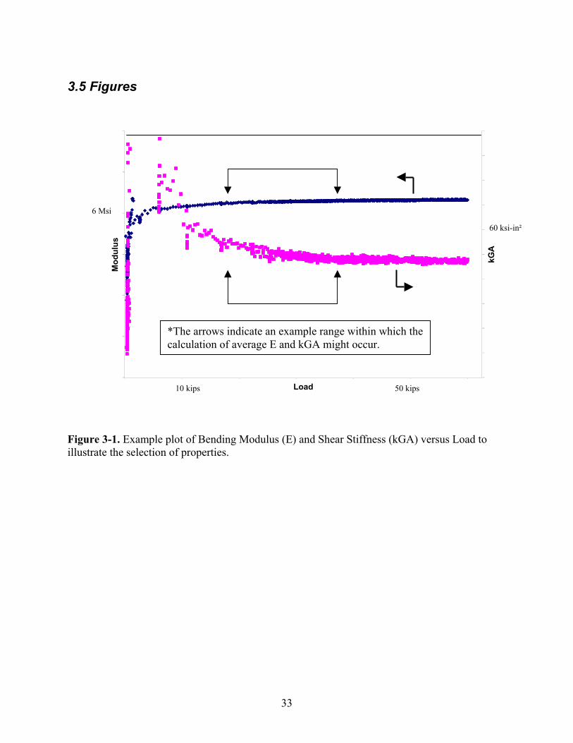
resistance............................................................................................................................... 16 Figure 2-1. 3-Point bend test setup for short span 8 in. DWB testing ......................................... 22 Figure 2-2. 8 in. DWB short span testing instrumentation plan ................................................... 22 Figure 2-3. Shear strain distribution in the web, at the neutral axis, of 8 in. DWB (P = 30 kips) 23 Figure 2-4. Shear capacity vs. L/d for 8 in. DWB and initial prediction for the 36 in. DWB...... 23 Figure 2-5. Typical delamination failure of 8 in. DWB obtained during short span testing ........ 24 Figure 2-6. Four-point bend setup for stiffness and strength testing of 36 in. DWB ................... 24 Figure 2-7. Schematic of load patch for 36 in. DWB testing ....................................................... 25 Figure 2-8. Instrumentation plan for testing of 36 in. DWB ........................................................ 25 Figure 3-1. Example plot of Bending Modulus (E) and Shear Stiffness (kGA) versus Load to
illustrate the selection of properties. ..................................................................................... 33 Figure 4-1. Typical load versus midspan deflection plot for 36 in. DWB (from a failure test) ... 42 Figure 4-2. Typical load versus end deflections plot of elastomeric bearing pads, F and B denote
that the displacement resulted at the front or back edge of the pad, respectively................. 42 Figure 4-3. Typical load versus midspan bending strains plot (stiffness test).............................. 43 Figure 4-4. Shear strain distribution in web, along neutral axis (9 inch wide load patch) ........... 43 Figure 4-5. Shear strain distribution in beam web, along neutral axis at an end support ............. 44 Figure 4-6. Typical plot of load versus far field shear strain in beam web .................................. 44 Figure 4-7. Top flange bending strain distribution across the width of the flange....................... 45 Figure 4-8. Compressive strain in beam web under a load point.................................................. 45 Figure 4-9. Typical plot of bending modulus (E) and shear stiffness (kGA) versus load ............ 46 Figure 4-10. Contribution of shear deformation to total beam deflection versus span (average
experimental E and kGA) ..................................................................................................... 47 Figure 4-11. Plot of kGA versus load comparing data calculated from an LVDT and a wire pot47 Figure 4-12. Modulus and kGA versus load calculated from wire pot data (System 6000)......... 48 Figure 4-13. Post-failure bending modulus versus load (80% of modulus retained) ................... 48 Figure 4-14. Typical delamination failure of 36 in. DWB ........................................................... 49 Figure 4-15. Bearing failure at supports for beam tested at L/d of 6............................................ 49 Figure 4-16. Schematic illustrating the three bearing pad orientations (BPO) used during testing
............................................................................................................................................... 50 Figure 4-17. Shear Capacity versus span for the 36 in. DWB (note that beams with an L/d of 6
did not fail in shear), BPO – bearing pad orientation ........................................................... 50 Figure 4-18. Ultimate capacity of 36 in. DWB broken down by manufacturing batch................ 51 Figure 4-19. Weibull mean and A- and B-basis allowables for bending modulus ....................... 53 Figure 4-20. Weibull mean and A- and B-basis allowables for shear stiffness............................ 53 Figure 4-21. Weibull mean and A- and B-basis allowables for shear capacity............................ 54 Figure 5-1. Wide flange glass FRP beam ..................................................................................... 68 Figure 5-2. WF beams with 0-, 1-, and 3-plies of unidirectional carbon bonded to flanges ........ 68
viii

Figure 5-3. WF beams shown in three spans tested (L/d of 6, 13, and 19) .................................. 69 Figure 5-4. Four-point bending test setup for WF beams............................................................. 69 Figure 5-5. Close-up of four-point bend test setup ....................................................................... 70 Figure 5-6. End view of four-point bend test setup ...................................................................... 70 Figure 5-7. Steel end support roller utilized for four-point bend setup ........................................ 71 Figure 5-8. Steel end support roller with top plate utilized for four-point bend setup ................. 71 Figure 5-9. Illustration of the differences between the theoretical and experimental shear
distributions in the web of an FRP beam.............................................................................. 72 Figure 5-10. Cross-sectional geometry of a WF beam used to determine shear correction factor72 Figure 5-11. Typical load versus deflection plot for four-point testing of WF section ................ 73 Figure 5-12. Typical load versus top and bottom flange midspan bending strains ...................... 74 Figure 5-13. Typical plot of bending modulus and shear stiffness versus load............................ 74 Figure 5-14. Plot of bending modulus and shear stiffness from 16-bit acquisition system data .. 75 Figure 5-15. Same beam as shown in Figure 5-14 tested using 12-bit acquisition system .......... 75 Figure 5-16. Ratio of EI/kGA versus span for all three beam types............................................. 77 Figure 5-17. Average kGA for each beam type versus span ........................................................ 77 Figure 5-18. Distribution of shear strain in beam web for no plies and 3-plies of carbon lamina 78 Figure 5-19. Contribution of shear deformation to the total beam deflection at test spans,
calculated using the average bending modulus and shear stiffness for each beam .............. 79 Figure 5-20. Distribution of shear strain in beam web for point load and load patch cases......... 79 Figure 5-21. Typical plot for determination of E and kGA from slope-intercept method............ 80 Figure 5-22. Span dependence of shear stiffness for beams with no carbon plies ....................... 82
ix
Chapter 1 Introduction and Literature Review
1.1 Introduction
Fiber-reinforced polymeric (FRP) composites are being considered for structural
members in civil infrastructure applications as lighter, more durable alternatives to steel and
concrete. The interest in these materials can be attributed to the ability of FRP to better meet the
performance and durability needs of current construction. Existing structural shapes include
wide-flange beams, box beams, sandwich beams, and multi-cellular panels. The constituent
materials of these structural components tend to be E-glass fibers and low cost resin systems
(polyester, vinyl ester, etc.). Occasionally, carbon fiber is utilized in flanges or face sheets in
order to increase bending stiffness. Construction typically utilizes off-the-shelf pultruded
sections or structural members may be manufactured using vacuum-assisted resin transfer
molding. A few of the benefits of FRP for use in infrastructure compared to conventional
materials are high strength to weight ratios, high corrosion resistance, lightweight,
electromagnetic transparency, and excellent fatigue performance.
The claim of FRP composites to have excellent long-term durability makes them well-
suited for infrastructure applications. The problem is that there are few documented cases in
literature to validate these claims. Some data from short-term laboratory projects is available.
However, it is difficult to make long-term generalizations since these studies typically involve
specific materials and conditions (environmental, loading, etc.). Some evidence of success can
be seen from marine and chemical storage applications, but data from these areas is difficult to
obtain as little actual documentation exists. The majority of information on the performance of
composite materials comes from the aerospace industry, an area where cost and long-term
durability are often of secondary importance. Additionally, the high performance applications of
the aerospace industry demand such materials as carbon fiber and epoxy resins. Construction
and civil infrastructure applications require the more cost competitive glass fibers and polyester
or vinyl ester resins, materials with less existing data available on performance.
The lack of long-term durability data has led to the slow acceptance of FRP composites
in the civil infrastructure community. There are also additional factors inhibiting widespread
1

use. Composites tend to have considerably higher initial costs than conventional engineering
materials (i.e. steel, concrete, wood, etc.). It is believed by advocates that composites will have
lower life-cycle costs due to their increased durability, but again the lack of long-term data has
left this claim not fully substantiated. Since composites are relatively new to the industry, the
lack of experience designing with these materials tends to drive initial costs higher yet. And
although the high stiffness-to-weight ratio of FRP composites makes them appealing for many
applications, the relatively low absolute stiffness of these materials causes difficulties in fully
utilizing their strength since most infrastructure design is deflection controlled. Additionally,
few standards for design and repair with composites are available. Some of the larger
manufacturers of composite structures are creating design manuals for their own products
independently, occasionally in conjunction with academic and government research groups.
Overall, composites continue to gain acceptance and find new roles in infrastructure
applications due to their numerous advantages. Along with the aforementioned benefits, the
lighter structures that are produced utilizing composites allow for increased live load capacities
on abutments and easier implementation in previously less accessible locations. In order to
continue to enhance approval in the infrastructure community, more long-term durability
information is required, the costs of constituent materials (especially carbon fiber) must continue
to decrease, and more field trials must be conducted. Demonstration and low-risk, small-scale
projects utilizing composites is perhaps the key to widespread acceptance. One such project
demonstrating the use of FRP composites in bridge applications is the replacement of the steel
stringer, timber deck bridge on Route 601 in Smyth County, Virginia.
1.2 The Route 601 Bridge
The former Route 601 Bridge (Figure 1-1) spanned 30 ft (9.1 m) across Dickey Creek in
rural, southwest Virginia (Marion, VA) and consisted of eight, 8 to 10 in. (203 to 254 mm) deep
steel girders. The Virginia Department of Transportation (VDOT)-owned structure was built in
1932 and was found to be in need of rehabilitation after a 1998 inspection due to excessive
corrosion. The site provided an excellent opportunity for a demonstration of an innovative
composite material superstructure.
2

The replacement bridge (Figure 1-2) was designed through collaboration by Virginia
Tech, Strongwell, Corp., the Virginia Transportation Research Council (VTRC) and VDOT.
The new structure spans 39 ft (11.8 m) from center-of-bearing to center-of-bearing and consists
of eight 36 in. (914 mm) double-web composite beams with a 42 in. (1.1 m) transverse beam
spacing. The span of the bridge was increased to account for the greater depth of the composite
beams to prevent any restriction of drainage. Ten, 4 ft long by 30 ft wide by 5 1/8 in. thick (1.2
m x 9.1 m x 130 mm) glue laminated timber panels make up the deck and the structure is topped
off with an asphalt wearing surface. Prior to the rehabilitation of the Route 601 Bridge, the
beams to be implemented in the new structure were tested quasi-statically to obtain stiffness data
and one beam was tested to failure. Since the completion of the rehabilitation, failure testing of
additional beams (19 beams in all) has also been completed. For further details on the design of
and girder proof testing for the Route 601 Bridge refer to the Virginia Tech Master of Science
Thesis by Waldron [23].
1.3 The 36 in. Hybrid FRP, Double-Web Beam (DWB)
The 36 in. (914 mm) FRP DWB (Figure 1-3) is manufactured by Strongwell, Corp. in
Bristol, Virginia by means of the pultrusion process. The hybrid beam is comprised of both glass
and carbon fibers in a vinyl ester resin matrix (Dow Chemical’s Derakane 411-350). Glass
roving, 0/90° and ±45° fabric, and continuous strand mat (CSM) are located throughout the
section and unidirectional carbon fiber tows are utilized in the flanges to increase the bending
modulus and to move the failure plane of the DWB away from the web-flange interface and into
the top flange. A fiber volume fraction of approximately 45% is targeted. The actual fiber lay-
up is proprietary, though the webs and flanges are basically quasi-isotropic with the flanges also
utilizing the unidirectional carbon fiber laminae. The unique shape of the beam was designed to
utilize the properties of composites. The double-webs and sub-flanges work to increase the shear
stiffness of the structure as well as increase resistance to lateral-torsional buckling. This increase
in shear stiffness is of great significance since shear deformation in composite materials cannot
be ignored as it can in steel and concrete structures. Shear deflection in these composite
3

structures can contribute as much as 15- and even 20% of the total beam deflection at spans that
are common to the type of bridges these beams were designed for.
During the development of the 36 in. DWB, an 8 in. (203 mm) (Figure 1-4) deep subscale
prototype was studied and implemented in the Tom’s Creek Bridge rehabilitation in 1997 [1].
The results of extensive testing of this section including stiffness and strength data have been
published in a structural design guide, published in 2000 [2]. As tested in three- and four-point
bending, the 8 in. DWB consistently fails by delamination within the compressive flange at the
interface between carbon and glass fibers. The critical stress in this case is thought to be the
normal, out-of-plane stress at the free edges. Furthermore, the delamination appears to initiate at
the load points, suggesting that load concentrations have a significant effect on the critical stress.
The failure mechanisms of the 36 in. DWB will be addressed in Chapter 4.
1.4 The 36 in. DWB Structural Design Guide
As it was previously stated, failure and stiffness testing has been conducted on a number
of 36 in. DWBs. The primary purpose of this testing is the development of a structural design
guide for the DWB, which will contain strength and stiffness data obtained during testing. The
design guide is presented as a material specification where the material system and the
manufacturing process are well defined and controlled. Knowing the tolerances of this system
and process, guidelines are defined for the use of the structural member. As a basis for defining
operating limits, a modified Load Resistance Factor Design (LRFD) approach is considered [3].
For this approach the probability distribution of loads/stress (Loads, Q) is compared to the
probability of failure strength of the material (Resistance, R), typically represented as illustrated
in Figure 1-5. The region of overlap is related to the risk associated with the situation designed.
Specifically in the design guide, the resistance portion of the design problem is presented by
employment of Weibull statistics [2, 25, 26] on test data. Weibull statistics help capture the
variability of materials by describing the probability of failure and tend to describe the
distribution of data for composite materials more accurately than a normal distribution. A
reliability based selection approach is used, from the recorded variability of girder test data, to
define A- and B-basis allowable levels of resistance. The Weibull statistics equations that are
4

used to calculate the A and B allowables can be found in Appendix A. An A-basis allowable
means that there is a 99% probability that the calculated value is within a 95% confidence
interval. Similarly, a B-basis allowable suggests that there is a 95% probability that the
calculated value falls within a 95% confidence interval. These values define for users of the
design guide the level of risk allowed in operating the structure based on a determined design
load. The difference between the selected design loads and the resistance (defined as a
probability of failure load/stress) defines the level of risk (or inversely the margin of safety) for
the design (Figure 1-5). The probability and confidence levels that are set for the A and B
allowables are determined by the Mil-17 Specification on composite materials [27].
The purpose of the design guide is to assist potential users of the DWB in specifying the
component in various structural applications. The content includes the specification of bending
stiffness, shear stiffness, shear capacity, moment capacity, lateral-torsional stability, bearing
capacity, and bolted connection specifications. An overview of the testing and results follows in
subsequent chapters.
1.5 Literature Review
A review of the literature has been conducted on the use of composite materials in
infrastructure, the status of infrastructure in the United States, and some issues that are restricting
the general acceptance of composites in the industry and this information is presented in the
following sections. In addition to this, a survey of literature on the characterization of shear
effects in composite structures, in particular shear stiffness, has also been conducted in order to
get a better understanding of this material property.
1.5.1 Status of U.S. Infrastructure
The deteriorating condition of the transportation infrastructure of the U.S. has become a
severe problem, especially considering the economic impact that the industry as on the national
economy. The value of the transportation infrastructure is said to be worth more than $2.5
5

trillion. In addition to this, about $900 billion annually or about 20% of the gross domestic
product comes from transportation related activities. Construction, maintenance, and operation
of the transportation network requires $120 billion in funding per year, with maintenance alone
drawing up nearly $100 billion [4]. One source estimated that by the year 2000, $50 billion per
year would be required for the maintenance of bridges [5]. This high requirement for bridge
maintenance costs is due to indications that approximately 4 to 10% of the Country’s 550,000+
bridges are considered to be in an advanced state of deterioration and over 30% are said to be
“structurally deficient” or “functionally obsolete”. As many as 200,000 bridges may need to be
rehabilitated over the course of this and the next decade [5]. Anywhere from $10 to $50 billion
or more annually will be required to keep up with this state of degeneration in U.S.
infrastructure, however only about $5 billion is budgeted for infrastructure improvement [6].
Since it is not always possible to build new roadways to avert the increasing demand of
traffic and to relieve congestion, the only remaining option is to make improvements to existing
structures. Small investments into ideas that promote research and education such as RIPE
(research, implementation, promotion, and education) can result in huge cost and efficiency
gains [4]. One source indicated that improving the durability of pavement by only 1% could
save $10 billion or much more in the next 20 years [4]. U.S. bridges are typically designed for a
life of 70 years and require rehabilitation at some time around mid-life due to deterioration.
Since the majority of bridges in the U.S. were built after 1945, it is inevitable that a large number
of replacements structures will have to be built in the next 10 to 20 years. And since the majority
of deterioration to existing bridge structures can be attributed to the corrosive environment
created by de-icing salts, there is additional motivation to invest time and resources into
researching and implementing new systems and materials more resistant to such environments
[5].
1.5.2 Composites in Infrastructure
The nearly routine use of FRP composites for such applications as aircraft structures and
even space shuttle components suggest that the composites industry has made great
advancements in design considerations. It should come as no surprise then that the success
6

attained in the aforementioned applications along with the advantageous features of these
materials is allowing them to carve out a niche in the infrastructure industry as well. And
although acceptance may be occurring at a rather slow rate, FRP composites are currently being
implemented in a number of civil and military infrastructure applications as experimental
projects and demonstrations [4].
There are additional motivations for civil engineers to explore new alternatives for bridge
design and materials as well. There has been some investment of effort into trying such things as
coatings and binders with traditional materials, but the majority of new interest is in exploring
composite materials as alternatives to steel, concrete, and timber. The concern for the state of
bridges in the near future combined with financial restraints has fueled this interest as there is a
need for new technologies [6].
There are numerous reasons why FRP composites are being utilized in civil and military
infrastructure. There obviously is also a rationale for why their adoption has been somewhat
slow. The lack of long-term durability data has already been mentioned as one of the primary
hindrances to FRP usage. The long-term degradation of FRP composites due to moisture, freeze-
thaw cycling, UV radiation, chemical state changes, etc. has been studied at various levels in
laboratories and in some field applications, but due to the limited use of most current composite
structures in civil applications, the long-term effects of these types of degradation are not yet
known. Moreover, most bridge designs are deflection controlled and the low stiffness of FRP
composites compared to steel can also limit their use. The large deformations that occur can
cause problems with concrete overlay and deck connections as well [6]. The addition of carbon
fiber as a means for stiffening glass-fiber composites can alleviate some of these problems, but
the high cost of the resulting hybrid structure is another obstacle.
Despite the limitations of FRP composites, engineers are finding ways to overcome these
factors and utilize their many advantages. For instance, although the relatively low absolute
stiffness of FRP composites is a limitation, the high strength- and stiffness-to-weight ratios make
them ideal for applications where the location is less accessible. A composite structure can
significantly reduce a bridge’s dead load allowing for an increased live load without abutment
strengthening and may also give the structure a larger load carrying capacity. One of the primary
advantages of FRP composites is they tend to be more corrosion resistant than metals. This
increased resistance can be attributed to the chemical stability and resistance to fatigue crack
7
growth that composites exhibit. Due to the light weight and durability of these materials, a
properly designed FRP bridge structure can weigh less, last as long or longer, reduce
maintenance costs, and have increased strength when compared to a steel or concrete bridge.
1.5.3 Issues and Characteristics of FRP Composites
As FRP composites continue to gain acceptance in the infrastructure community, they are
finding additional roles in new applications as both secondary and primary load bearing
members. Some of the applications currently utilizing composites include guard rails,
diaphragms, column wrapping, reinforcement of concrete beams, reinforcement and repair of
steel members and splice plates, and as a method of protecting joints and bridge bearings from
various environmental factors [5]. The potential also exists for use as bridge beams and decks as
a means for improving durability, but to this point the majority of instances for this type of role
has been as demonstration projects and experimental cases. The FRP composites that are
typically being utilized tend to be the more cost-effective glass-fiber, polyester resin or glass-
fiber, vinyl ester resin combinations. In some instances, carbon fiber is also being utilized when
the need for increased mechanical properties (e.g., bending stiffness) can offset some of the
deterring higher costs. One of the more popular methods for manufacturing these composite
structures, especially in large-scale applications and production, is the pultrusion process. The
relatively simple, cost-effective, flexible, continuous nature of this process makes it ideal for
manufacturing infrastructure components. As constituent materials, pultrusion generally utilizes
a combination of fiber rovings, stitched fabrics, and continuous and chopped strand mats
resulting in relatively low fiber volume fractions of about 40 to 55% [6]. Resin infusion and
resin transfer molding are also occasionally used to produce infrastructure components, but these
processes are more common in cases where customization is needed or prototype structures are
required [7].
There continues to be an increasing demand for guidelines and standards to follow in the
design and implementation of FRP composite structures. The American Society for Testing and
Materials (ASTM) and such organizations as the American Concrete Institute (ACI) and the
American Association of State Highway Transportation Officials (AASHTO) are a few of the
8

institutions addressing these needs. In addition to these groups, as it was mentioned previously,
various component suppliers and manufacturers, including Strongwell Corp., Hardcore
Composites, and Creative Pultrusions, are also independently developing design guides for their
own products to assist users in the proper use of those products. Clearly defined and easily
accessible guidelines are necessary to assist those utilizing composite components that have
limited experience with FRP composites. It is also important that these guidelines include
methods for reducing structural properties over time and deal with the possibility that the failure
mode of the structure may change in time as well [8].
As it was mentioned, there are a few cases where independent product manufacturers
have developed design guides for their own products. Not only is Strongwell Corp. in the
process of developing such a manual for the 36 in. DWB as this document is outlining, they also
have already published a guide for the 8 in. DWB, as mentioned, and provide another such
publication for their EXTREN family of structures, which includes a variety of pultruded
structural shapes [9]. Hardcore Composites of New Castle Delaware provides a design guide for
composite tubular piles. This guide (available over the internet) contains explanations for use
and typical applications of the piles, as well as such design properties as bending stiffness (EI)
and ultimate bending moment, including the computational methods utilized [10]. Another
pultruder of structural shapes, Creative Pultrusions, also has an online design guide for their
structural shape product line, Pultex. This guide provides physical and mechanical properties,
load tables, environmental considerations, fabrication and quality assurance information, as well
as additional information regarding the use of their product [11].
In addition to the abovementioned design manuals provided by independent companies,
there are also a number of guides provided by governmental organizations. The EUROCOMP
design code and handbook for design with polymer composites exists to provide specifications
for structural design of composites in European countries [28]. The Japan Society of Civil
Engineers (JSCE) has published a comprehensive guide for the proper design and construction of
concrete structures reinforced using composite materials. This 300+ page document provides
guidelines for such things as design basics, material specifications, and load tables to ultimate
conditions, serviceability conditions, and fatigue information, as well as other information [12].
The previously mentioned ACI has developed a design manual for designing concrete structures
using FRP rebar [13].
9

1.5.4 Shear Effects in FRP Structures
There is not an abundance of literature available on shear effects in FRP structures. And
very little of what is available specifically involves the study of shear stiffness (kGA), the
importance of which will be discussed for the 36 in. DWB in later chapters. Some information is
available on shear deformable beam theories, the shear correction factor (k) (primarily for beams
with rectangular cross-sections), the influences of shear in sandwich composites, and the effects
of shear lag and warping.
For sandwich composites, the determination of shear stiffness is explained using the
potential energy of applied loads and balancing that with the strain energy of the system. And
this theory is extended for cases where typical sandwich conditions do not apply (modulus of the
core << modulus of the flanges, which is the weak core assumption, thin face assumption, etc.)
[14]. The influence of shear effects in isotropic beams was first proposed by Timoshenko in
1921 in order to correct his first order beam theory to account for the shear effects. He rederived
the results a year later using an approach based on elasticity. In this second paper, the shear
correction factor, k, was introduced to take into account the non-uniform distribution of shear
across a structure’s cross-section. The first accepted definition for k was the ratio of the average
shear strain through the cross section to that at the centroid, but this definition proved to give
poor results and the definition was revised. A possible, more accurate definition for k is given
by one source as the ratio of shear area to the cross-sectional area of the beam [15].
In 1966, Cowper [16] derived the shear coefficient using three-dimensional elasticity
equations. This approach was extended to thin-walled sections consisting of orthotropic
composite laminates in the late 1980’s [17]. In this last approach, the effect of out-of-plane
Poisson’s ratio is neglected and only the in-plane mechanical properties of the lamina that make
up the beam are utilized. There are a handful of other sources that derive and extend the
relationship for the shear correction factor for such cases as nonsymmetric, orthotropic laminates
[18]; rectangular beams with arbitrary lay-ups [19]; cases where the Poisson’s ratio effect is
important [15], and similar cases in Bank, Pai et al., and Barbero et al. [20, 21, 22].
10
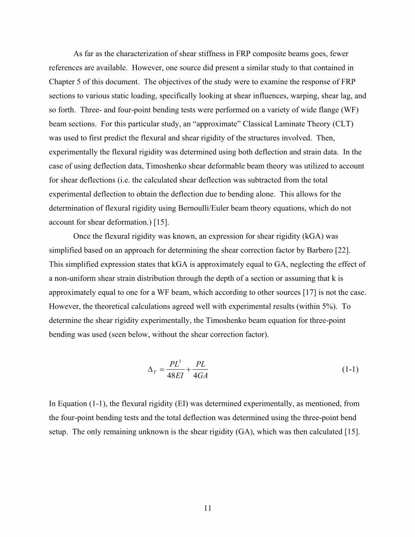
As far as the characterization of shear stiffness in FRP composite beams goes, fewer
references are available. However, one source did present a similar study to that contained in
Chapter 5 of this document. The objectives of the study were to examine the response of FRP
sections to various static loading, specifically looking at shear influences, warping, shear lag, and
so forth. Three- and four-point bending tests were performed on a variety of wide flange (WF)
beam sections. For this particular study, an “approximate” Classical Laminate Theory (CLT)
was used to first predict the flexural and shear rigidity of the structures involved. Then,
experimentally the flexural rigidity was determined using both deflection and strain data. In the
case of using deflection data, Timoshenko shear deformable beam theory was utilized to account
for shear deflections (i.e. the calculated shear deflection was subtracted from the total
experimental deflection to obtain the deflection due to bending alone. This allows for the
determination of flexural rigidity using Bernoulli/Euler beam theory equations, which do not
account for shear deformation.) [15].
Once the flexural rigidity was known, an expression for shear rigidity (kGA) was
simplified based on an approach for determining the shear correction factor by Barbero [22].
This simplified expression states that kGA is approximately equal to GA, neglecting the effect of
a non-uniform shear strain distribution through the depth of a section or assuming that k is
approximately equal to one for a WF beam, which according to other sources [17] is not the case.
However, the theoretical calculations agreed well with experimental results (within 5%). To
determine the shear rigidity experimentally, the Timoshenko beam equation for three-point
bending was used (seen below, without the shear correction factor).
GAPL
EIPL
T 448
3
+=∆ (1-1)
In Equation (1-1), the flexural rigidity (EI) was determined experimentally, as mentioned, from
the four-point bending tests and the total deflection was determined using the three-point bend
setup. The only remaining unknown is the shear rigidity (GA), which was then calculated [15].
11

1.5.5 Summary
The status of the transportation infrastructure in the United States reveals that there is a
need for technological changes in the industry in order to correct for the deteriorating conditions
of bridges and roadways. The potential for composite materials to help reverse this trend has
been shown. Their advantages over traditional materials, in particular their high stiffness- and
strength-to-weight ratios, long-term durability, and corrosion resistance has enabled them to
begin creating a niche in the civil infrastructure community, although there acceptance is still
slowed by some of the uncertainties and disadvantages previously mentioned. The need for
design guides and standards was noted as one factor in particular that needs to be addressed and
it is the purpose of this research to address that concern.
1.6 Problem Statement
To date, there are few guidelines and standards available to assist users with the proper
design of FRP structures for civil infrastructure applications. The need for such has been
discussed and the need for structures, materials, and technology that will aide in the
rehabilitation of the transportation infrastructure of the United States has also been established.
Additionally, there is limited information available on the influence of shear effects on FRP
girders, with very little of what is available dealing specifically with shear stiffness. It is the
intent of this research to add to what is available regarding the characterization of shear effects in
FRP composite structures, as well as assist in the development of a structural design guide for
the 36 in. DWB. It is believed that this hybrid composite structure has the ability to provide a
durable, corrosion resistant alternative to steel and concrete for the efficient rehabilitation of
relatively short span bridges across the country.
There were two primary goals for this research. The first goal was to characterize the
properties of the 36 in. DWB for specification in a structural design guide. This was done by
conducting stiffness and strength testing of the girder to determine such attributes as bending
stiffness, shear stiffness, and ultimate load limits at a number of spans. The A and B basis
allowables were determined for each of these properties for the design manual. Failure modes
12

were investigated. The second goad was to investigate shear effects in the DWB and in other
FRP structures as it is believed these effects are not fully understood. In order to better
understand shear effects, a model study was conducted on additional, smaller FRP structures to
supplement the data obtained for the DWB and to further examine some of the factors thought to
contribute to the variation seen in shear stiffness.
13

1.7 Tables and Figures
Figure 1-1. Former Route 601 Bridge
Figure 1-2. New Route 601 Bridge with 36 in. DWBs
14
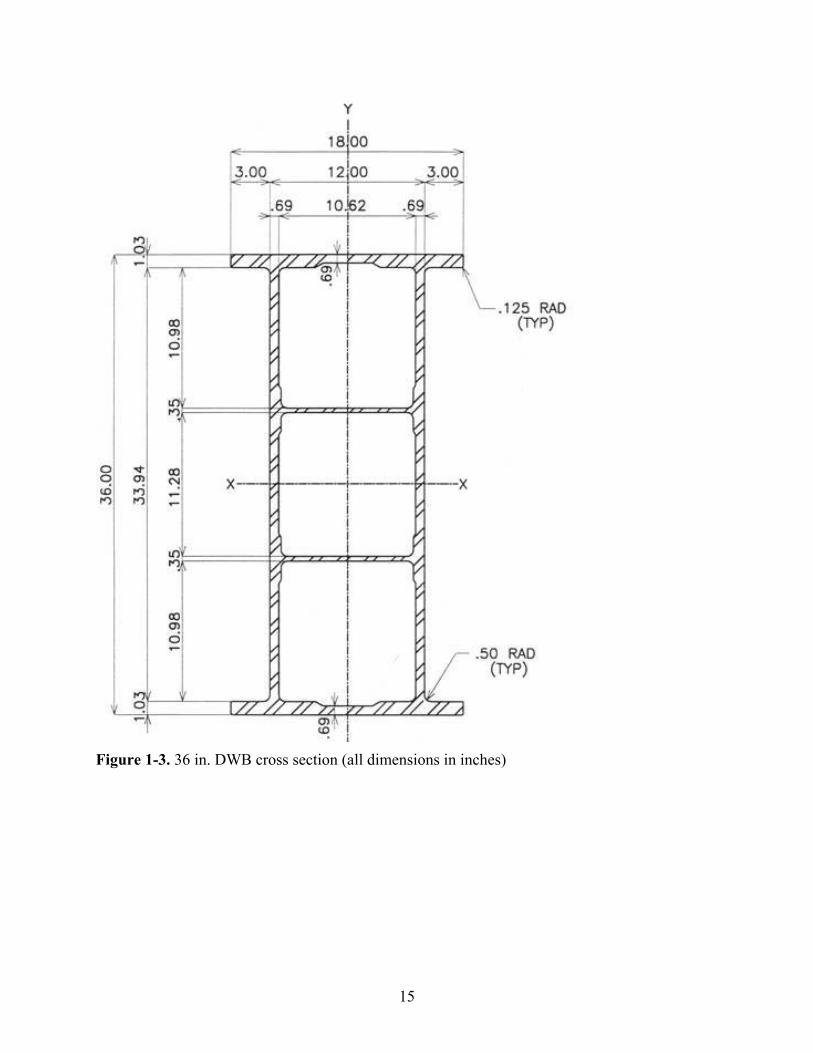
Figure 1-3. 36 in. DWB cross section (all dimensions in inches)
15

Figure 1-4. 8 in. DWB cross-section (all dimensions in inches)
Load, QResistance, R Resistance, R
A-Basis
B-Basis
Level of Risk Figure 1-5. LRFD conceptual representation for design; A- and B-basis allowable levels of resistance
16

Chapter 2 Experimental Testing Procedures
2.1 Material System: Double-Web Composite Beams
As it was previously mentioned, the testing of two double-web beams (i.e. the 8 in. and
36 in. DWBs) has led to the development of a structural design guide for the 36 in. (914 mm)
DWB (Figure 1-3). During the development of the 36 in. DWB, an 8 in. (203 mm) deep
subscale prototype (Figure 1-4) was studied and implemented in the Tom’s Creek Bridge
rehabilitation in 1997 [1]. The results of extensive testing of this section including stiffness and
strength data have been published in a structural design guide, published in 2000 [2]. The 8 in.
DWB, like the 36 in. girder, is a combination of glass roving, 0/90° and ±45° fabric, and CSM
with unidirectional carbon fiber laminae in top and bottom flanges embedded in Dow Chemical’s
Derakane 411-350 vinyl ester resin.
2.2 8 in. DWB Short Span Testing
An explanation of the testing conducted on the 8 in. DWB follows. Select results will
also be presented in this section as they were utilized to establish a plan for testing the 36 in.
DWB. Values in tables and figures are presented in U.S. Customary units as they will appear in
the structural design manual.
As a precursor to the aforementioned strength testing of the 36 in. DWB, a number of
tests were performed on the 8 in. DWB. Preliminary results from strength testing the 8 in. DWB
indicated that the moment to failure varied with span. In order to further examine the
contribution of span (and therefore shear) to the failure of the 8 in. DWB, a number of three-
point, short-span failure tests were performed. Spans of 16, 32 and 60 inches (406, 813, and1524
mm), corresponding to 2, 3 and 7.5 times the depth of the beam, were chosen. Data at longer
spans of 8, 14 and 17.5 feet (2.4, 4.3, and 5.3 m), length-to-depth ratios of 12, 21 and 26,
17

respectively, had been previously collected. For the short beam tests, three beams of each length
were loaded to failure in a three-point bend test geometry (Figure 2-1). A 6 in. (152 mm) square,
1 in. (25 mm) thick elastomeric bearing pad was used at the load point (and similar, thinner pads
at the end supports) to distribute the load evenly; and a 1 in. (25 mm) thick steel plate under the
actuator was also utilized. The ends were restrained to prevent any lateral translation.
Deflection was measured at mid-span using a wire potentiometer. Shear strain in the web near
the loading point was measured in one test at each span with strain gages placed at a ±45°
orientation along the neutral axis of the beam in order to examine the effect of a concentrated
load on the local stress field, i.e. the degree to which cross-sectional warping affects the flange
stresses. Beginning underneath the load patch at mid-span, shear gauges were placed every 1.5
in. (38 mm) extending out at least one pad’s width from the beam center after which every 3 to 6
in. (76 to 152 mm) of spacing was utilized until the beam end was reached. The gauge plan and
set-up can be seen in Figure 2-2.
One area of interest in the short span testing of the 8 in. DWB was to establish the
distance from the load patch that was required for shear strain in the beam web to become a
constant value, i.e., the shear lag. As a result of prior testing, it was thought that this distance
was equal to one width of the load pad. To further evaluate these results, a 6 in. (152 mm) load
pad was used. A plot of shear strain versus position (Figure 2-3) shows that at a distance of 6
inches (152 mm) from mid-span (the center of the load pad), the shear strain in the beam web
appears to reach a constant value. This particular plot is for a load of 30 kips (133 kN), but the
relationship remained the same at all loads. The arrows on the plot indicate the edge of the load
pad and the distance required for shear strain to become constant (one pad width), respectively.
The primary purpose of this short span testing was to establish the dependence on span of
the shear capacity of the 8 in. DWB and use that information to predict the capacity of the 36 in.
DWB. The shear capacity of the 8 in. beam versus the length-to-depth ratio, as well as the
original projection for the 36 in. beam can be seen in Figure 2-4. This projection was made
using a ratio of the capacity for the 8 in. DWB to the one experimentally determined strength of
the 36 in. DWB (i.e. the capacity of the 39-ft (11.9 m) girder failed prior to the rehabilitation of
the Route 601 Bridge) and then extending this relationship for the other known values of the 8 in.
DWB. The purpose of developing the projection was to determine the spans at which to conduct
stiffness and failure tests of the 36 in. DWB.
18

The final point of interest in the testing of the 8 in. DWB was an analysis of the failure
mechanism. As tested in three- and four-point bending (the four-point bending tests were
conducted during the development of the aforementioned structural design guide), the 8 in. DWB
consistently fails by delamination within the compressive flange at the interface between carbon
and glass fibers. The critical stress in this case is thought to be the normal, out-of-plane stress at
the free edges. Furthermore, the delamination appears to initiate at the load points, suggesting
that load concentrations have a significant effect on the critical stress. A picture of a typical
failure obtained during testing can be seen in Figure 2-5.
2.3 36 in. DWB Stiffness and Strength Testing
As it was explained in the previous section, short span failure testing of the 8 in. DWB
was conducted, among other reasons, to determine at which spans the 36 in. DWB would be
evaluated for the purpose of obtaining material properties for a structural design guide. After
considering the capacity of the test set-up available and the projection seen in Figure 2-4, spans
of roughly 20, 40, and 60 ft. (6.1, 12.2, and 18.3 m) were selected as it was thought that these
spans would provide sufficient data to determine the relationship between shear capacity and
span. Due to various factors on the laboratory floor (e.g. available space, bolt hole locations,
reaction floor length, etc.), the spans at which the girders were actually initially tested were 18,
39, and 58 ft. (5.5, 11.9, and 17.7 m), which correspond to length-to-depth ratios (L/d) of 6, 13,
and 19 1/3, respectively. Seventeen girders (five to six beams at each span from three different
manufacturing batches) were initially scheduled to be tested and failed. After testing girders at
the aforementioned spans, additional beams at a span of 30 ft (9.1 m), an L/d of 10, were also
tested for reasons that are discussed in Chapter 4.
For the stiffness and failure testing of the 36 in. DWB, a four-point bending setup was
utilized. The test setup involves two hydraulically driven 400 kip (1779 kN) actuators located at
the third points with two 9- by 14-in. (229 by 356 mm) long elastomeric bearing pads (used to
mimic bridge applications) at both the supports and the loading points (Figure 2-6). Also at the
load points, in an attempt to more evenly distribute the load across the entire width of the beam,
the load is delivered onto 2 in. (51 mm) thick steel plates welded to small, reinforced steel I-
19

beams (Figure 2-7). The boundary conditions provided by the elastomeric bearing pads are
considered to be the same as or very similar to that of a simply supported beam since the pads
allow both rotation and lateral translation through axial compression and shear deformation of
the pads. Additionally, displacement was measured at the midspan of each beam and at the
quarter points for the 60-foot span using wire potentiomers and, for stiffness tests, the more
precise ±1 in. (±25 mm) Linear Variable Displacement Transformer (LVDT). The end
deflections (which occur due to the use of the elastomeric bearing pads) at the supports were also
measured using LVDTs and subsequently subtracted from midspan deflections to find the net
deflection of the girder.
A variety of different strain gauging plans were implemented on the different beams of
each span. On every beam, three gauges were evenly spaced across the top and bottom flange at
midspan to measure bending strain and axial gauges were placed on the web along the neutral
axis to monitor for any warping in the beam. As with the 8 in. DWB, shear strain in the web was
also measured in the proximity of the load points and supports for beams at each span to examine
the effect of a concentrated load on the local stress field. On various beams, strain gauges were
positioned at different locations on the girders in an attempt to measure a variety of different
beam characteristics. For instance, bending strains were measured a distance of 1 in. (25 mm)
from the load point to further examine the effects of a concentrated load, gauges were placed
vertically in a grid-like pattern on the web under a load point to look into the presence of any
web compression or warping, and other similar attempts were made to better understand the
complexities of a double-webbed composite beam. On a number of beams crack gauges were
also used in an attempt to better characterize the failure mode of the 36 in. DWB. An
instrumentation diagram can be seen in Figure 2-8.
Testing of each beam began with low load stiffness testing. The magnitude of the load
for this testing was limited by the stroke (approximately 1.25 in. (32 mm)) of the LVDT located
at midspan. This was necessary in order to obtain the most accurate deflection data possible.
Once stiffness testing was completed, the centrally located LVDT was removed and the beams
were loaded and unloaded to progressively higher loads until failure occurred. For safety
reasons, lateral restraints were placed on the beam on each side of both load points, all test
equipment was secured in some manner to the test frame, a Plexiglas shield was placed between
the beam and test engineer (i.e. the author), and the lab was evacuated. Due to the large amount
20

of energy released by the beams at the moment of failure and the high loads involved, these
precautions were deemed necessary and if nothing else gave some peace of mind to the test
engineer loading the beam (the author).
Once failure testing was completed, a post-failure inspection was conducted to examine
the method of failure (to be discussed later in Chapter 4), examine residual deflection and
deformation, conduct post-failure loading (one beam), and document cracks and delaminations.
21
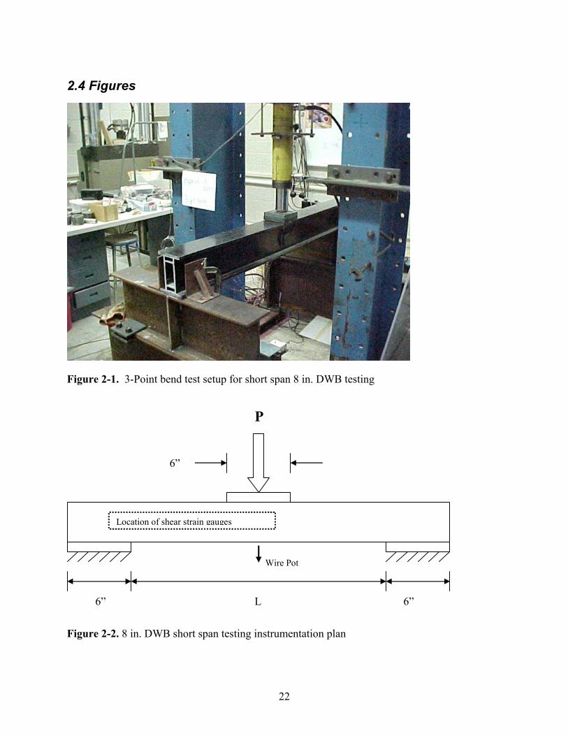
2.4 Figures
Figure 2-1. 3-Point bend test setup for short span 8 in. DWB testing
P
6”
6” 6” L
Location of shear strain gauges
Wire Pot
Figure 2-2. 8 in. DWB short span testing instrumentation plan
22

0
1000
2000
3000
0 3 6 9Distance from Load Patch Center (inches)
Stra
in (m
icro
stra
in)
12
32 in. Span60 in. Span
Shear strain appears to reach a constant level
Pad edge
Figure 2-3. Shear strain distribution in the web, at the neutral axis, of 8 in. DWB (P = 30 kips)
0
40
80
120
0 5 10 15 20 25 30L/d
Shea
r Cap
acity
(kip
s)
8 in. DWBLinear (8 in. DWB)Linear (PROJECTED 36 in.)
Obtained from failure testing of 39 ft. beam
Figure 2-4. Shear capacity vs. L/d for 8 in. DWB and initial prediction for the 36 in. DWB
23
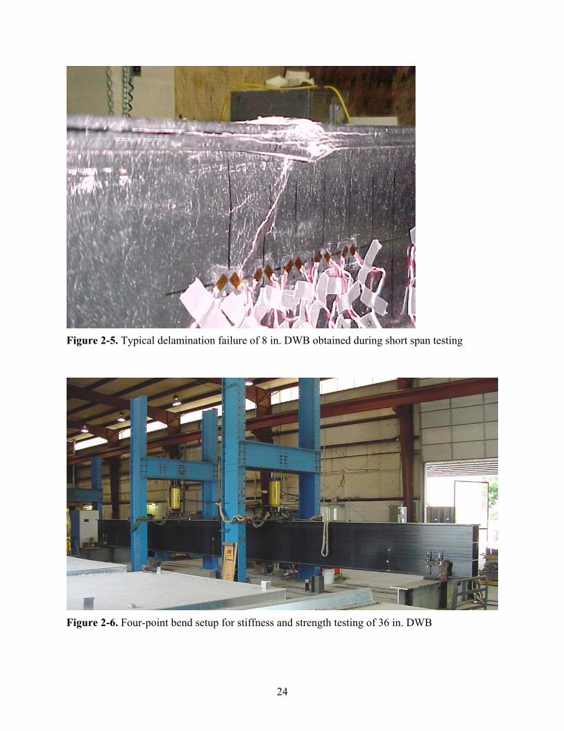
Figure 2-5. Typical delamination failure of 8 in. DWB obtained during short span testing
Figure 2-6. Four-point bend setup for stiffness and strength testing of 36 in. DWB
24
14”
DWB
bearing padsteel plate
Stiffened WF beam
Actuator
14”
DWB
bearing padsteel plate
Stiffened WF beam
Actuator
14”
DWB
bearing padsteel plate
Stiffened WF beam
Actuator
14”
DWB
bearing padsteel plate
Stiffened WF beam
Actuator
14”
DWB
bearing padsteel plate
Stiffened WF beam
Actuator
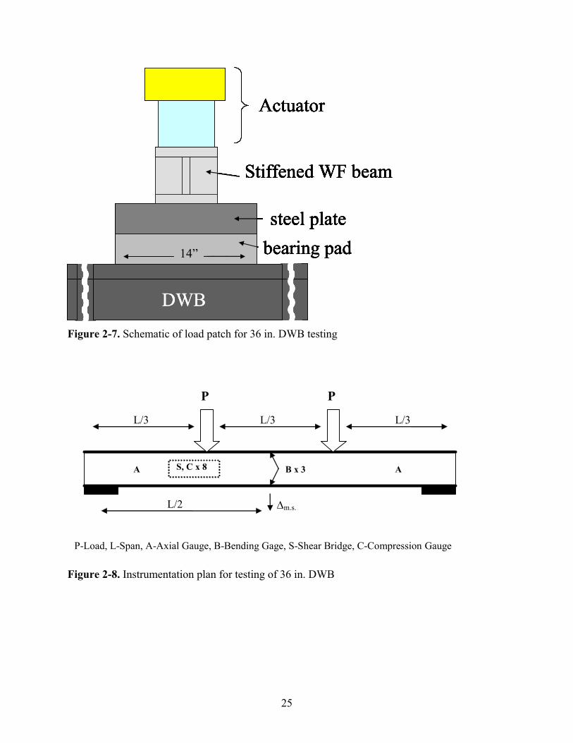
Figure 2-7. Schematic of load patch for 36 in. DWB testing
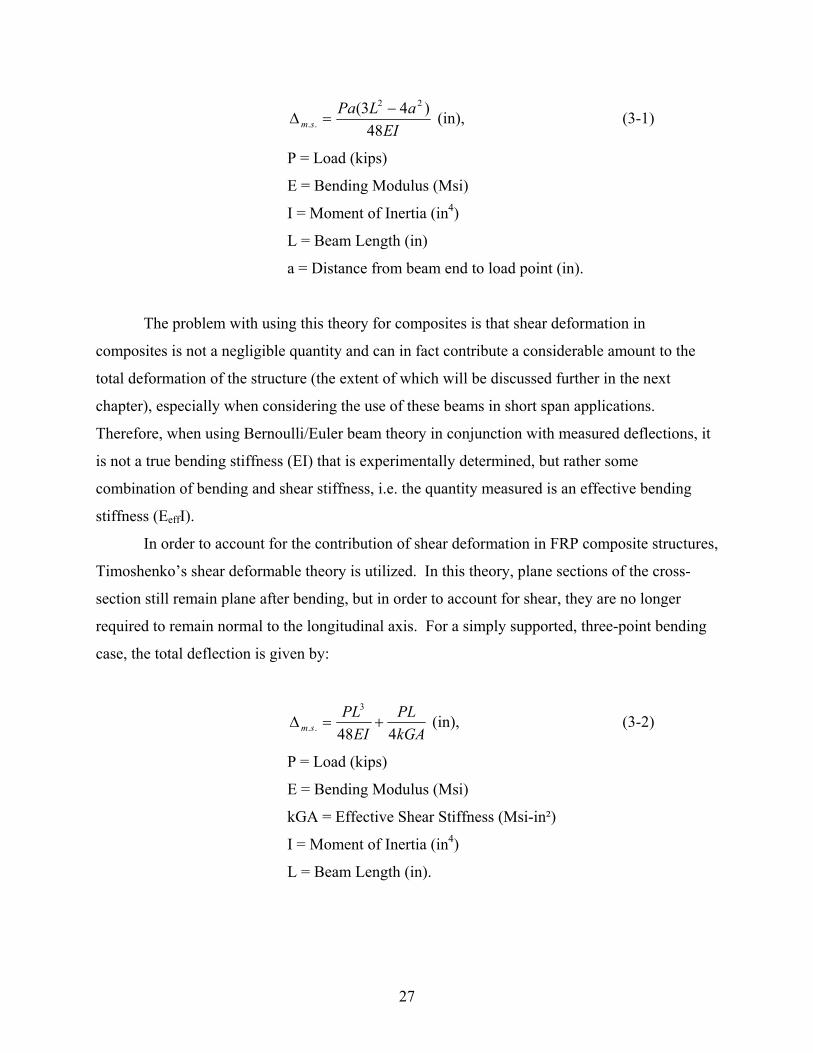
A AB x 3 S, C x 8
L/3 L/3 L/3
L/2 ∆m.s.
P P
P-Load, L-Span, A-Axial Gauge, B-Bending Gage, S-Shear Bridge, C-Compression Gauge
Figure 2-8. Instrumentation plan for testing of 36 in. DWB
25

Chapter 3 Analysis Procedures
After testing of the 36 in. (914 mm) DWB was complete, the next step was to perform an
analysis of the collected data. Nineteen beams were tested, according to the methods discussed
in the previous chapter, in order to determine the strengths and stiffnesses that will assist future
users of this structure by helping to form the structural design guide for this member. The results
of analyzed data are presented in Chapter 4. The methods used to determine those results are
presented here in the sections to follow.
3.1 Beam Stiffness Characterization
Each of the nineteen beams tested were done so in order to first determine their bending
modulus (E) and shear stiffness (kGA). Bending stiffness (EI) is the property more commonly
used by civil engineers. In this case, since the moment of inertia (I) was known, the two terms
will be separated. For a typical bridge type structure with conventional materials, the deflection
of a beam under transverse loads can be accurately characterized using only EI. For materials
like steel and concrete in typical infrastructure applications, Bernoulli/Euler beam theory, which
does not account for shear deformation, is used for analysis since deformation due to bending
controls the response of the structure and shear deformations are negligible [23].
In Bernoulli/Euler beam theory, beam cross-sections that are plane and normal to the
longitudinal axis prior to bending remain plane and normal during bending. The following
equation (Equation 3-1) is the midspan deflection of a simply supported beam loaded at a
distance “a” from one end:
26
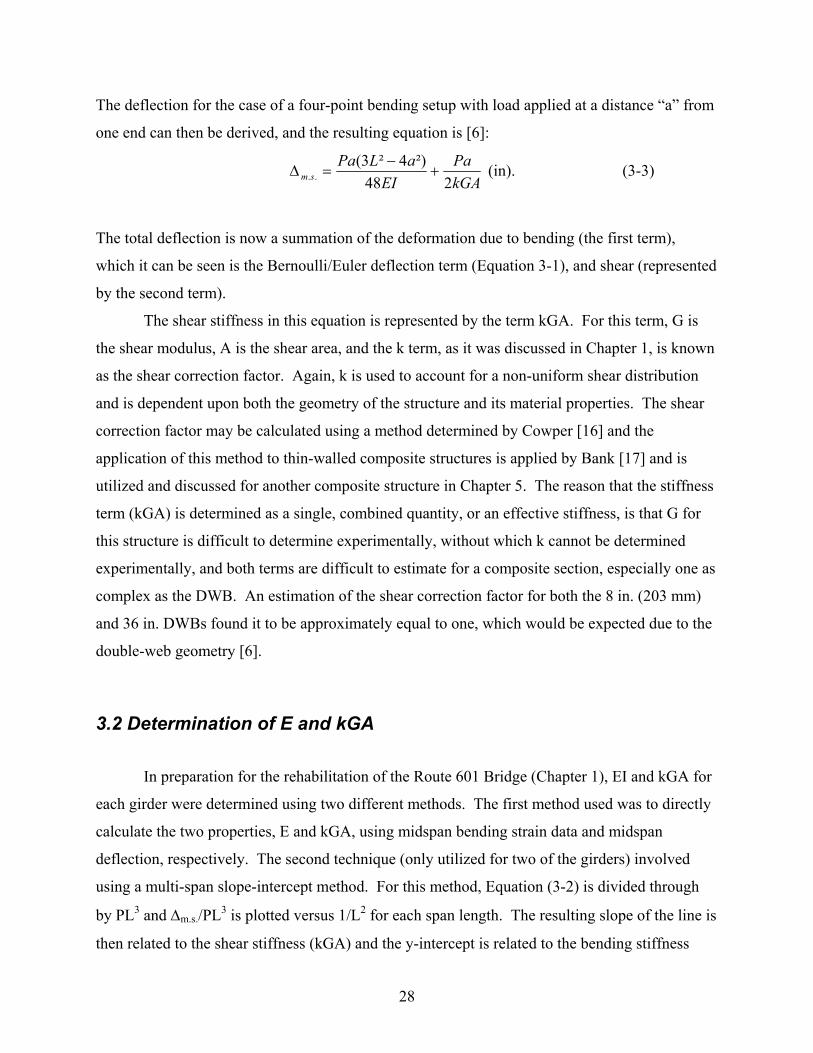
EI
aLPasm 48
)43( 22
..−
=∆ (in), (3-1)
P = Load (kips)
E = Bending Modulus (Msi)
I = Moment of Inertia (in4)
L = Beam Length (in)
a = Distance from beam end to load point (in).
The problem with using this theory for composites is that shear deformation in
composites is not a negligible quantity and can in fact contribute a considerable amount to the
total deformation of the structure (the extent of which will be discussed further in the next
chapter), especially when considering the use of these beams in short span applications.
Therefore, when using Bernoulli/Euler beam theory in conjunction with measured deflections, it
is not a true bending stiffness (EI) that is experimentally determined, but rather some
combination of bending and shear stiffness, i.e. the quantity measured is an effective bending
stiffness (EeffI).
In order to account for the contribution of shear deformation in FRP composite structures,
Timoshenko’s shear deformable theory is utilized. In this theory, plane sections of the cross-
section still remain plane after bending, but in order to account for shear, they are no longer
required to remain normal to the longitudinal axis. For a simply supported, three-point bending
case, the total deflection is given by:
kGAPL
EIPL
sm 448
3
.. +=∆ (in), (3-2)
P = Load (kips)
E = Bending Modulus (Msi)
kGA = Effective Shear Stiffness (Msi-in²)
I = Moment of Inertia (in4)
L = Beam Length (in).
27
The deflection for the case of a four-point bending setup with load applied at a distance “a” from
one end can then be derived, and the resulting equation is [6]:
kGAPa
EIaLPa
sm 248²)4²3(
.. +−
=∆ (in). (3-3)
The total deflection is now a summation of the deformation due to bending (the first term),
which it can be seen is the Bernoulli/Euler deflection term (Equation 3-1), and shear (represented
by the second term).
The shear stiffness in this equation is represented by the term kGA. For this term, G is
the shear modulus, A is the shear area, and the k term, as it was discussed in Chapter 1, is known
as the shear correction factor. Again, k is used to account for a non-uniform shear distribution
and is dependent upon both the geometry of the structure and its material properties. The shear
correction factor may be calculated using a method determined by Cowper [16] and the
application of this method to thin-walled composite structures is applied by Bank [17] and is
utilized and discussed for another composite structure in Chapter 5. The reason that the stiffness
term (kGA) is determined as a single, combined quantity, or an effective stiffness, is that G for
this structure is difficult to determine experimentally, without which k cannot be determined
experimentally, and both terms are difficult to estimate for a composite section, especially one as
complex as the DWB. An estimation of the shear correction factor for both the 8 in. (203 mm)
and 36 in. DWBs found it to be approximately equal to one, which would be expected due to the
double-web geometry [6].
3.2 Determination of E and kGA
In preparation for the rehabilitation of the Route 601 Bridge (Chapter 1), EI and kGA for
each girder were determined using two different methods. The first method used was to directly
calculate the two properties, E and kGA, using midspan bending strain data and midspan
deflection, respectively. The second technique (only utilized for two of the girders) involved
using a multi-span slope-intercept method. For this method, Equation (3-2) is divided through
by PL3 and ∆m.s./PL3 is plotted versus 1/L2 for each span length. The resulting slope of the line is
then related to the shear stiffness (kGA) and the y-intercept is related to the bending stiffness
28
(EI). For the design guide beams (i.e. the beams tested in this study), only the method of
calculating E and kGA from strain and deflection data was utilized. The values of bending and
shear stiffness calculated from the slope-intercept method did not agree well with those values
calculated directly from strain and deflection data in the Route 601 Bridge girder study so the
method was temporarily abandoned for the design guide beams. A study where the multi-span
slope-intercept method is reinvestigated is presented in Chapter 5.
3.2.1 Determination of Bending Modulus (E)
The bending modulus for the 36 in. DWB was calculated directly from top and bottom
flange axial bending strain data collected at the midspan of each beam. A four-point bending
setup was utilized so that a constant moment region would exist, i.e. the region between the
loading points. Theoretically, no shear strain exists in this region so the measured strain is a
result of pure bending. Solving the well-known relationship for stress and strain then gives the
equation used to calculate E:
εI
McE = (Msi), (3-4)
M = Moment (kip-in)
c = Centroidal Distance (in)
I = Moment of Inertia (in4)
ε = Average of Flange Strains (in/in).
3.2.2 Determination of Shear Stiffness (kGA)
After obtaining the bending modulus, shear stiffness (kGA) could then be calculated
using the midspan deflection data. For the testing of the 36 in. DWB, the load is applied at the
third points of the beam. Thus, substituting L/3 for “a” into the Timoshenko beam deflection
equation (Equation (3-3)) of a simply supported beam loaded in four-point bending and
superimposing the results for the two loads gives the resulting midspan deflection seen below:
29

kGAPL
EIPL
sm 364823 3
.. +=∆ (in). (3-5)
The only unknown in the equation is now kGA so Equation (3-5) can now be solved for
the shear stiffness.
−∆
=
EIPL
PLkGA
xm 648233
3
..
(ksi-in²) (3-6)
At this point, equations for kGA for each test geometry (i.e. the four different spans
tested) were derived. Rearranging and substituting in for each span gives the following
equations:
L = 704 in. (17.9 m)
a = 232.5 in. (5.91 m): PEI
EIPkGAsm 196946565163720
.. −∆= (ksi-in²), (3-7)
L = 477 in. (12.1 m)
a = 160.5 in. (4.08 m): PEI
EIPkGAsm 3100571181284
.. −∆= (ksi-in²), (3-8)
L = 360 in. (9.14 m)
a = 120 in. (3.05 m): PEI
EIPkGAsm 1656000120
.. −∆= (ksi-in²), (3-9)
L = 225 in. (5.72 m)
a = 76.5 in. (1.94 m): PEI
EIPkGAsm 32758838612
.. −∆= (ksi-in²). (3-10)
30

The lengths that are used above to derive Equations (3-7) through (3-10) are the spans at which
the 36 in. DWB was tested. The span is defined for analysis purposes as the distance between
the centers-of-bearing of the beam. For example, a beam with a clear span of 39 ft. (11.9 m) or
468 in. with a 9 in. (229 mm) long bearing pad relative to the length of the beam would have a
resulting span of 468 in. plus two times 4.5 in. (114 mm), or 477 in. (12.1 m).
3.3 Determination of E and kGA for the Structural Design Guide
To date, the method being implemented to determine and select the values of bending
modulus (E) and shear stiffness (kGA) for the structural design guide of the 36 in. DWB is as
follows. From the data collected during stiffness testing, the instantaneous E and kGA are
calculated for each sampled point of load, bending strain, and midspan deflection (sampling rate
is approximately 10 samples/second). The values over a set range of deflections were then
selected and the average of E and kGA at those points is taken. The deflections that were chosen
correspond to eleven evenly spaced values between the L/600 and L/800 deflection criteria, i.e.
the deflections at L/600, L/620, L/640,…, L/780, and L/800 (beam lengths must be in inches).
The L/800 criterion was selected as it is specified for bridge design by AASHTO [3]. The
method of taking the average of these eleven points versus the average of the entire range
between the end points was chosen because it was found that it was as accurate as and
considerably more efficient than the latter method.
The L/600 and L/800 criteria were chosen for two reasons. It was decided that
consistency was most important in selecting E and kGA, so a range of deflections had to be
chosen that could be reached at each span. Therefore, the controlling factors became the stroke
of the midspan LVDT responsible for measuring deflection and the length of the longest span.
At the 704 in. (17.9 m) span, the resulting deflection at the L/600 criteria is approximately 1.2 in.
(30 mm), which is roughly the upper limit of the linear range of the LVDT used to measure
deflection. Since it is necessary to calculate kGA using the more accurate LVDT deflection data
(versus that of a wire potentiometer), the deflection of the beam at the L/600 criteria became the
upper limit of the range. Though bending modulus does not depend upon deflection, this
property was also taken from the same range for consistency. The reason that both properties
31

had to be selected from any range at all and not just averaged over the course of the entire test
can easily be seen from a plot of E and kGA versus load (Figure 3-1). As the plot demonstrates,
E and kGA do not reach a constant value instantaneously so a range must be selected in order to
obtain a representative value of each material property. More will be discussed regarding the
nature of these properties for the 36 in. DWB in Chapter 4.
Once the selection of E and kGA was complete, the remaining step was to use Weibull
statistics to determine the A and B allowables for each value. For details on Weibull statistics
refer to Chapter 1 and Appendix A.
3.4 Strength Testing Analysis
As described in Chapter 2, after stiffness testing was conducted on each beam for the four
different spans, each 36 in. DWB was then loaded with progressively higher loads until failure
occurred. This was done to obtain ultimate strength data, as well as to investigate the
dependence of capacity upon span with the primary purpose being for specification in the
structural design guide for the 36 in. DWB. And again, Weibull statistics were employed to the
capacities of the beam to calculate A and B allowables for each span. In addition to the
collection of strength data, moment to failure was calculated for each beam, maximum deflection
(∆m.s., max) and maximum bending strain (εb, max) were documented, and a physical analysis of the
failure was conducted, all of which was done to explore the possibility of existing trends.
32
3.5 Figures
2000000
3000000
4000000
5000000
6000000
7000000
8000000
0 20 40 60 80 100 120
Load
Mod
ulus
0.00E+00
1.00E+07
2.00E+07
3.00E+07
4.00E+07
5.00E+07
6.00E+07
7.00E+07
8.00E+07
9.00E+07
1.00E+08
kGA
6 Msi
60 ksi-in²
*The arrows indicate an example range within which the calculation of average E and kGA might occur.
10 kips 50 kips
Figure 3-1. Example plot of Bending Modulus (E) and Shear Stiffness (kGA) versus Load to illustrate the selection of properties.
33

Chapter 4 Experimental Results and Discussion
As it has been discussed in the preceding chapters, the nineteen DWBs provided by
Strongwell, Corp. were tested with the primary purpose of obtaining stiffness and strength data
for the development of a structural design guide for the 36 in. (914 mm) DWB. The testing
involved two main components: low-load stiffness testing for beam property characterization and
failure testing to determine ultimate shear capacity and failure mode. In addition to the
characterization of these traits, testing was also conducted to investigate a number of other beam
attributes including, shear strain transfer characteristics in the web, shear lag effects in the
flange, moment capacity, strain to failure, etc. The results of both portions of testing follow in
the next few sections. In this chapter, values in tables and figures are presented in U.S.
Customary units as they will appear in the structural design manual.
4.1 Stiffness Testing
The first portion of the design manual testing was low-load stiffness testing to determine
the bending modulus (E) and shear stiffness (kGA). Following the procedures described in
Chapter 2, each beam was loaded to approximately 20 to 100 kips (89 to 445 kN), depending on
span, as was limited by the stroke of the deflection measuring equipment (i.e. the LVDT).
4.1.1 Beam Response
As in the testing previously conducted on the 36 in. DWB for the rehabilitation of the
Route 601 Bridge, all girders demonstrated a linear-elastic response. Plots of load versus
midspan deflection were generated for each test. A typical load versus deflection plot can be
seen in Figure 4-1 and a typical plot of the end deflections due to the compressibility of the
elastomeric bearing pad (measured at the four corners of the pad) can be seen in Figure 4-2.
Also for each test, midspan bending strains on the top and bottom flange were recorded at three
34
evenly spaced points across the width of the beam and the average for each flange was
computed. A plot of load versus the resulting average bending strains is presented in Figure 4-3.
As was previously mentioned, one point of interest in the testing of the 36 in. DWB was
the investigation of shear strain transfer in the web of the beam. For one to two beams at each
span, shear strain was measured in the web of the beam along the neutral axis in the proximity of
both the load points and end supports. The original hypothesis based on the testing of the 8 in.
(203 mm) DWB was that the lag in shear strain transfer (i.e. the distance required for the shear
strain in the web to reach a constant value) was related to the width of the loading pad. For the
short span testing of the 8 in. beam, a 6 in. (152 mm) load patch was used and the results appear
to support the claim (Figure 2-3). However, according to Dufort [24], the transfer length may
also be a function of the depth of the beam. For the 36 in. DWB, both cases can be argued
(Figure 4-4). In the plot of shear strain versus position (Load = 80 kips (356 kN)), the shear
strain appears to reach a constant value (or at least it appears to have stopped increasing) after a
distance equivalent to one pad width extending out in the direction of the end supports. On the
other hand, the strain between the load points appears to require approximately 18 in. (457 mm)
before it reaches zero (recall that the constant moment region is theoretically absent of shear
effects), which is a distance that could be related to the depth of the beam. And again in Figure
4-5 it can be seen that more than the distance of one pad width is required to reach a constant
value, this time in the region around an end support. Essentially, a case can typically be made
for both possibilities. For this reason, future testing is planned to further investigate shear strain
transfer. Load versus far-field shear stress was also plotted to ensure its linearity (Figure 4-6).
In addition to examining shear strain in the web of the beam, there were a number of
other beam responses that were examined using the various strain gauge configurations discussed
briefly in Chapter 2. The distribution of bending strains across the width of the flange near one
of the load points was measured and compared to those measured at midspan. A plot of these
strains and their locations on the flange may be seen in Figure 4-7. From the plot it does not
appear that there is any distinct effect of a concentrated load on the bending strains.
Compressive strains in the web under the load patch were also recorded (Figure 4-8). As a
means to gauge their magnitude, note that the bending strain at the same load (60 kips or 267
kN) during the test from which this data was taken was approximately 300 microstrain as well.
One area where the compression of the web becomes significant is in the stress analysis of the
35

structure. The beam web is generally considered to be incompressible, but this data suggests that
this may not be the case for this structure.
4.1.2 Bending Modulus (E) and Shear Stiffness (kGA)
The bending modulus (E) and shear stiffness (kGA) for each beam were calculated
directly from midspan bending strain and deflection data, respectively, according to the methods
described in Chapter 3. A typical plot of E and kGA versus load for a low load test can be seen
in Figure 4-9. The flat nature of the curve for E and the non-constant nature of kGA were
common to most every test. A summary of the values of E and kGA for each beam can be seen
in Table 4-1. The reported values of both of these properties are obtained from taking the
average for each for multiple tests. The calculated values for the majority of the individual load
tests may be seen in Appendix B.
As it can be seen from the plot of kGA versus load (Figure 4-9), shear stiffness appears to
decrease as the beam is loaded. This is the opposite case from what was measured during the
testing of the beams for the Route 601 Bridge rehabilitation [23]. In that case kGA appears to
increase as additional load was applied. Timoshenko beam theory (refer to Chapter 3) suggests
that kGA, or G in particular, is a material property and should therefore be independent of load
and remain constant, as the bending modulus appears to be. To date, this phenomenon is
unexplained and is being studied further. There are a number of possible reasons for this and the
variation in general that can be seen in the reported values of kGA, as well as the variation that
can be seen in Figure 4-9. First of all, although Timoshenko, unlike Bernoulli/Euler beam
theory, does account for shear deformation, it does so in a relatively simple manner. A more
complex theory to capture the deformation may be needed.
One reason in particular that the accurate characterization of the shear deformation of the
36 in. DWB is important is that, especially at short spans, the contribution of shear deformation
to the total deflection becomes a significant portion (Figure 4-10). In fact, in preparation for the
rehabilitation of the Route 601 Bridge, it was calculated using the conservative values of E and
kGA that were used for the bridge’s design that shear deflection accounted for 16 percent of the
36
total deflection of the structure [23]. Using the average experimentally determined values of E
and kGA reveals that this portion is smaller, but remains important nonetheless.
It has been found that shear stiffness is extremely sensitive to numerous factors,
especially the midspan deflection from which it is directly calculated. For example, it has
already been mentioned that kGA is calculated using deflections measured using LVDTs due to
the increased accuracy they provide versus wire potentiometers. A plot comparing the property
measured using each can be seen in Figure 4-11. In addition to the displacement transducer type,
the resolution of the acquisition system is another key to measuring accurate deflections and thus
reducing variation in kGA calculations. Mid-way through the testing of beams, the computer
running the acquisition system crashed due to old age and was beyond repair. This acquisition
system had been chosen due to its familiarity to users, but the computer crash required a change
to a newer system with better resolution. The data collected using this system, as would be
expected, proved to be more noise-free and more accurate. Figure 4-12 shows a plot of E and
kGA from this system. This data was even calculated using the measurements from a wire-
potentiometer, which with the old system, it would have been extremely difficult to obtain usable
data. The importance of acquisition system resolution is demonstrated further in Chapter 5.
Another important point is illustrated by the plot of E and kGA versus load in Figure
4-12. The plot illustrates the problem in accurately reporting kGA when the data is taken from
the low load ranges that were selected for consistency purposes in the design guide. The
advantage of being able to accurately measure deflection up to failure loads or at least over a
larger range is quite evident.
Along with the ability to accurately measure deflection, there are other factors
contributing to the variation that can be seen in kGA. For instance, the span that is selected for
analysis can contribute to the uncertainty in shear stiffness. The decision to select center-of-
bearing to center-of-bearing as opposed to clear span impacts the value of kGA, not only because
it goes directly into the calculation of E in the form of a moment arm, but also because it changes
the coefficients in the Timoshenko shear deformable beam theory equations that are derived for
the calculations (refer to Chapter 3).
This issue was of particular importance for the 18 ft (5.49m) span because the boundary
conditions were different for each of the three beams tested for reasons that will be explained in
the next section. For the short span, the center-of-bearing to center-of-bearing distance had to be
37

adjusted, which resulted in variations in both the bending moduli (especially relative to that of
the other three spans) and also shear stiffnesses. And though two of the calculated values
obtained for kGA are very close in magnitude, a close examination of the data shows that this
may be only due to chance variation as well. These two beams had distinctly different boundary
conditions (explained in the next section), different center-of-bearing to center-of-bearing spans,
the largest difference between values of bending modulus of any of the combinations of beams
within a span, and the largest difference between any two failure loads of any combination
within a span, which suggests that the shear strains are most likely quite different although no
shear gauges were present on either beam to confirm this speculation. Basically, it is the belief
of the author that these two values are as good an indication of the variability of kGA as is the
difference between the shear stiffness of these two beams and the third at this span, which it
should be noted had the largest calculated value of kGA of any of the beams (note that due to the
boundary conditions for this beam, it had end deflections due to the elastomeric bearing pads that
were over three times that of any other beam).
There are other, more difficult to quantify factors that may contribute to the variations in
kGA and the difficulties that are had in accurately characterizing this property. For instance, the
load being applied through a load patch to the flange most likely has an effect (again, boundary
conditions), the existence of significant compressive strains in the web (suggesting that the web
may not be incompressible), material nonlinearities, and the shear lag that was discussed in the
previous section (also discussed further in Chapter 5) is also most definitely contributing to the
variation in and/or difficulty in measuring the shear stiffness of this structure.
4.2 Strength Testing
Once low load stiffness testing was complete for each beam, the straightforward process
of strength testing was performed. The beams were simply loaded until they failed in some
manner. The typical failure was accompanied by an explosive burst of sound, and was also
defined by the sudden drop in load (though the shock wave was all that was necessary to signal
failure). The beams provide little warning before failure in most cases, but although it is loud, it
would not be considered catastrophic. In fact, post-failure testing of one beam showed the
38
ability to hold load and revealed that over 80% of the bending modulus (E) was retained (Figure
4-13).
As it was seen in the plot of shear capacity versus aspect ratio, there appears to be a linear
relationship between shear capacity and span for the 8 in. DWB (Figure 2-4). Initial testing of
the larger girder at the 39 and 58 ft (11.9 and 17.7 m) spans supported the hypothesis that the 36
in. DWB would behave in a similar fashion. Furthermore, the failure mechanism did not change
at these two spans, just as it did not with the 8 in. girder. The 36 in. DWB appears to fail in a
similar manner to the 8 in. DWB, which consistently fails by delamination in the top flange at a
carbon-glass interface (an area of high interlaminar stress due to the differences in the modulus
of the two materials), beginning in the vicinity of the loading patches and progressing outward in
both directions along the primary beam axis. For the 36-inch DWB, delamination may also
initiate at the internal ply drop-off underneath the flange (refer to Figure 1-3). This drop-off is
the result of glass fabrics in the outer half of each web that fold over in the pultrusion die to form
the inner half of each flange. Tests using crack detection gauges to capture the path of crack
growth along the length of the beam were attempted. The results supported the idea that the
delamination began at a load point, but due to the speed of the crack growth (and relatively slow
acquisition speed of the system used), little else was able to be determined from the data. A
picture of a typical delamination failure can be seen in Figure 4-14.
Testing for the 36 in. DWB began at the 58 ft span, progressed to the 39 ft girders, and
then finally to the 18 ft (5.5 m) beams. As it was mentioned, testing of the two longer spans
supported the original hypothesis that failure was controlled by shear capacity, that this shear
capacity varied linearly with span, and that the failure mechanism remained was independent of
span. Testing of the 18 ft DWBs revealed that this was not exactly the case. Three 18 ft, 36 in.
DWBs were tested and all three failed by a different failure mechanism than the previously
tested girders. It seems that shear capacity is not the only controlling factor as bearing failures
occurred in all three of the 18 ft beams. The bearing failures occur at the end supports as a result
of the elastomeric bearing pads creating additional stresses on the flanges, causing cracking at
the web-flange junction. In the worst case, the crack propagated up the web of the beam, causing
it to buckle as seen below in Figure 4-15.
Three different orientations of the elastomeric bearing pads were tried (one on each of the
three girders tested), as it was thought that the original alignment created an upward stress on the
39

flange edge that was causing the cracking at the web-flange junction. The original pad
orientation (used for the 39- and 58 ft spans) was such that the pads stuck out 5 in. (127 mm) on
each side of the beam, relative to the 18 in.(457 mm) width of the beam (the pads were 9 in. (229
mm) along the length of the beam and 28 in. (711 mm) across the width). The second orientation
turned the pads so that they went from flange edge to flange edge (14 in.(356 mm) along the
beams length, 18 in. (457 mm) across the width). It was thought that this might alleviate some of
the stress on the flange edges; testing revealed that it did not. On the third and final 18 ft girder
tested, only one bearing pad was used, centered under the beam so that the pad edges lined up
exactly with the webs of the beam (14 in. (356 mm) across the width) and was 9 in. (229 mm)
along the length of the beam. The bearing failure seen in Figure 4-15occurred under this
boundary condition. The orientation of the bearing pads for each girder can be seen in Figure
4-16.
After it was discovered that a bending-type failure (delamination of the top flange) could
not be obtained at the short 18 ft span, an additional failure test of a DWB at a 30 ft (9.1 m) span
was conducted. The bearing pads were oriented in the same manner as the second 18 ft test (18
in. (457 mm) wide, 14 in. (356 mm) along the length of the beam) and the beam did indeed fail
by delamination in the top flange, the same mode as those of the two longest spans. Four
additional beams provided by Strongwell Corp. were then tested at a span of 30 ft and all failed
in the same manner as the first (i.e. top flange delamination). The testing of the 30 ft. span
concluded the strength and stiffness portion of the design manual testing. The resulting plot of
shear capacity versus aspect ratio may be seen for the 36 in. DWB in Figure 4-17. It must be
noted that beams with an aspect ratio of 6 did not fail due to shear capacity and are therefore
represented on the plot as individual data points. It also would not be representative to plot the
average of those three tests, as the test geometries (boundary conditions) were quite different due
to the dissimilar bearing pad orientations. A table showing a summary of the results of all the
strength testing, as well as the stiffness testing, may be seen in Table 4-1.
In the summary table, the column headed “Batch” refers to which of the three pultrusion
runs that particular girder belongs (Batch 1—Summer 2000, Batch 2—May 2001, Batch 3—July
2001). The ultimate capacity (broken down by batch in Figure 4-18) was the total load of the
two actuators that the beam supported at failure and the shear capacity is the average of that
resulting sum. Again, E is the bending modulus and kGA is the shear stiffness. The data that
40
was lost for maximum bending strain and deflection was a result of the aforementioned problems
with the initial acquisition system. It should also be noted that the maximum deflections that are
presented are net deflections (i.e. midspan deflection minus the average of the end deflections).
It may also be of interest to note that for the first 18 ft girder listed, the relatively low net
deflection of only 0.8 in. (20 mm) was a result of that particular bearing pad orientation (only
one pad was used) causing an average end deflection of 0.5 in. (13 mm). A quick calculation of
kGA using a deflection of midspan deflection minus only half of the average end deflection
placed the value of kGA at approximately 35 to 40 Msi-in² (1560 to 1780 GPa-cm²). It is
difficult to judge if this is a more or less accurate estimation of shear stiffness, but it may not be
unreasonable to assume that the true value lays somewhere in between this estimation and the
reported value.
4.3 A and B Allowables for the Structural Design Guide
As it has been mentioned previously, Weibull statistics will be employed to determine A
and B allowables for E, kGA, ultimate shear strength, and moment to failure and the resulting
values will be presented in the structural design guide for the 36 in. DWB. The purpose of
reporting these values is that they are used to capture the variability in test data more thoroughly
than does a normal mean and standard deviation and also to define with what certainty or
confidence a given value may be used. A table summarizing the results of the Weibull
calculations (refer to Appendix A for details) can be seen in Table 4-3. The Weibull mean along
with the A and B allowables for bending modulus, shear stiffness, and shear capacity plotted
versus span can also be seen in Figure 4-19, Figure 4-20, and Figure 4-21, respectively.
41

4.4 Tables and Figures
0
20
40
60
80
100
120
140
0 1 2 3 4 5 6 7 8
Deflection (in.)
Load
(kip
s)
Figure 4-1. Typical load versus midspan deflection plot for 36 in. DWB (from a failure test)
0
90
0
Load
(kip
s)
1 2
Figure 4-2. Typithat the displacem
B1
0.0
cal load vent resul
B2
4 0.08End Deflection (in.
ersus end deflections ploted at the front or back e
42
F
0.12)
t of elastomeric dge of the pad, re
F
2
2
B1bearspe
B
F1
FLongitudinal direction of beam
0.16
ing pads, F and B denote ctively

0
10
20
30
40
50
-800 -600 -400 -200 0 200 400 600 800Strain (microstrain)
Load
(kip
s)Top FlangeBottom Flange
Figure 4-3. Typical load versus midspan bending strains plot (stiffness test)
-500
-400
-300
-200
-100
0-4.5 0 4.5 9 13.5 18 22.5
Distance from Pad Center (in.)
Stra
in (m
icro
stra
in)
80 kips
Constant Moment Region
Figure 4-4. Shear strain distribution in web, along neutral axis (9 inch wide load patch)
43

-600
-500
-400
-300
-200
-100
0
100
-18 -9 0 9 18 27
Distance from Support Center (in.)
Stra
in (m
icro
stra
in)
80 kips
Figure 4-5. Shear strain distribution in beam web, along neutral axis at an end support
0
50
100
150
200
250
0 200 400 600 800 1000 1200 1400Shear Strain (microstrain)
Load
(kip
s)
*Bending strain at 200 kips was approximately 1400
Figure 4-6. Typical plot of load versus far field shear strain in beam web
44

2500
2750
3000
3250
3500
0 4.5 9 13.5Distance from Flange Edge
Ben
ding
Str
ain
(mic
rost
rain
)
18
Near Load PointMidspan
*Strains @ 150 kips.
Figure 4-7. Top flange bending strain distribution across the width of the flange
0
5
10
15
20
25
30
-400 -300 -200 -100 0 100compressive strain (microstrain)
heig
ht a
bove
bot
tom
flan
ge (i
nche
s)
under load
4.5 inches fromedge of pad
60 kips
ε33 ,
0
5
10
15
20
25
30
-400 -300 -200 -100 0 100compressive strain (microstrain)
heig
ht a
bove
bot
tom
flan
ge (i
nche
s)
under load
4.5 inches fromedge of pad
60 kips
ε33 ,
0
5
10
15
20
25
30
-400 -300 -200 -100 0 100compressive strain (microstrain)
heig
ht a
bove
bot
tom
flan
ge (i
nche
s)
under load
4.5 inches fromedge of pad
60 kips
0
5
10
15
20
25
30
-400 -300 -200 -100 0 100compressive strain (microstrain)
heig
ht a
bove
bot
tom
flan
ge (i
nche
s)
under load
4.5 inches fromedge of pad
60 kips
ε33 ,
Figure 4-8. Com
pressive strain in beam web under a load point
45

0
2
4
6
8
0 10 20 30 40 50Load (kips)
Mod
ulus
(Msi
)
0
25
50
75
100
kGA
(Msi
-in^2
)EkGA
Figure 4-9. Typical plot of bending modulus (E) and shear stiffness (kGA) versus load
Table 4-1. Summary table of results of 36 in. DWB testing
L/d BatchShear
Capacity (kips)
Ultimate Capacity
(kips)
Mfailure
(kip-ft)Max dms
(in.)Max ( )
E (Msi)
kGA (Msi-in2)
6 3 156.0 312 994.5 0.80 2090 6.67 66.96 2 195.0 390 1283.8 1.31 2510 7.27 33.96 3 134.5 269 857.4 1.43 1850 6.52 33.610 1 121.5 243 1215.0 2.71 2540 6.70 47.310 3 129.0 258 1290.0 2.86 2830 6.44 43.410 3 143.0 286 1430.0 3.15 3205 6.38 49.110 3 143.5 287 1435.0 3.01 3090 6.63 50.310 3 138.0 276 1380.0 3.01 2985 6.52 62.413 3 113.5 227 1518.1 5.14 3440 6.27 44.513 3 72.0 144 963.0 3.27 2200 6.21 51.613 3 83.0 166 1110.1 6.02 58.513 3 106.5 213 1424.4 4.72 3150 6.49 47.213 1 117.0 234 1564.9 5.10 3570 6.61 39.513 1 81.5 163 1090.1 3.65 2570 6.28 46.2
19.33 2 82.5 165 1598.4 9.89 3660 6.40 53.519.33 2 73.5 147 1424.1 9.35 3170 6.66 52.319.33 2 59.0 118 1143.1 7.75 2620 6.45 38.019.33 3 60.5 121 1172.2 8.10 2620 6.37 42.119.33 3 66.5 133 1288.4 8.84 2930 6.39 43.9
lost data
b ε
µε
46

0
10
20
30
5 10 15L/d
% S
hear
Def
orm
atio
n
20
E = 6.43 MsikGA = 48.1 Msi-in²*Average values from test results
Figure 4-10. Contribution of shear deformation to total beam deflection versus span (average experimental E and kGA)
0
25
50
75
100
0 10 20 30 40 5Load (kips)
kGA
(Msi
-in^2
)
0
LVDTWire Pots
Figure 4-11. Plot of kGA versus load comparing data calculated from an LVDT and a wire pot
47

0
2
4
6
8
0 50 100 150 200 250 300Load (kips)
E (M
si)
0
25
50
75
100
kGA
(Msi
-in^2
)EkGA
*Approximate region from which E and kGA are selected for the design guide (L/600 to L/800 deflection criteria).
Figure 4-12. Modulus and kGA versus load calculated from wire pot data (System 6000)
0
2
4
6
8
0 5 10 15 20 25Load (kips)
Mod
ulus
(Msi
)
Pre-FailurePost-Failure
*Over 80% of Bending Modulus (E) was retained.
Figure 4-13. Post-failure bending modulus versus load (80% of modulus retained)
48

Figure 4-14. Typical delamination failure of 36 in. DWB
Figure 4-15. Bearing failure at supports for beam tested at L/d of 6
49

Top View
DWB DWB DWB
z z
1 2 3
Figure 4-16. Schematic illustrating the three bearing pad orientations (BPO) used during testing
0
50
100
150
200
3
Shea
r Cap
acity
(kip
s)
*Bearing FailuresBPO 2
Figure 4-17. Shdid not fail in s
BPO 3
6 9 12 15 18L/d
*Original Projection
BPO 1
ear Capacity versus span for the 36 in. DWB (note that beams with an L/d of 6 hear), BPO – bearing pad orientation
50

0
100
200
300
400
5 7 9 11 13 15 17 19L/d
Ulti
mat
e C
apac
ity (k
ips)
Batch 1 (Summer 2000)Batch 2 (May 2001)Batch 3 (July 2001)
Figure 4-18. Ultimate capacity of 36 in. DWB broken down by manufacturing batch
51

Table 4-2. Summary of Weibull statistics data
L/d = 10 E (Msi)
kGA (Msi-in²)
Shear Capacity (kips)
Moment Capacity (kip-ft)
Mean 6.52 50.3 134.4 1344.4Std. Dev. 0.16 8.5 11.7 116.8A Allowable 5.95 25.5 96.4 964.0B Allowable 6.23 35.7 113.9 1139.1α 50.21 7.0 14.1 14.1β 6.60 53.8 139.5 1395.0
L/d = 13 E (Msi)
kGA (Msi-in²)
Shear Capacity (kips)
Moment Capacity (kip-ft)
Mean 6.30 47.7 95.4 1275.8Std. Dev. 0.26 7.4 21.9 293.5A Allowable 5.43 25.9 36.8 492.8B Allowable 5.86 35.2 59.1 790.1α 30.98 7.7 5.0 5.0β 6.41 50.8 103.9 1389.9
L/d = 19.33 E (Msi)
kGA (Msi-in²)
Shear Capacity (kips)
Moment Capacity (kip-ft)
Mean 6.44 45.6 68.1 1319.2Std. Dev. 0.18 8.0 11.4 220.6A Allowable 5.82 22.4 34.7 672.7B Allowable 6.13 31.8 48.5 939.5α 45.65 6.7 7.0 7.0β 6.52 48.8 72.8 1409.9
52

0
2
4
6
8
8 10 12 14 16 18 20L/d
E (M
si) Mean
A AllowableB Allowable
Figure 4-19. Weibull mean and A- and B-basis allowables for bending modulus
0
20
40
60
8 10 12 14 16 18L/d
kGA
(Msi
-in^2
)
20
MeanA AllowableB Allowable
Figure 4-20. Weibull mean and A- and B-basis allowables for shear stiffness
53

0
40
80
120
160
8 10 12 14 16 18 2L/d
Shea
r Cap
acity
(kip
s)
0
MeanA AllowableB Allowable
Figure 4-21. Weibull mean and A- and B-basis allowables for shear capacity
54
Chapter 5 Investigation of kGA in FRP Beams
5.1 Introduction and Purpose
As it was discussed in Chapter 4, the characterization of shear stiffness (kGA) in the 36
in.(914 mm) DWB can be less than straightforward. The wide range of factors that contribute to
its variation have created a great deal of difficulty in accurately obtaining values from test data
and have led to an increase in the uncertainty in these calculated values. Moreover, results from
the testing of the 36 in. beam indicated that measured kGA values were in fact structural
properties, dependent upon the test geometry and setup itself. For these reasons, it was decided
to conduct a parametric investigation into the shear stiffness of FRP composite beams. It is
believed and has been shown in many cases that some of the factors that significantly affect the
value of and the ability to measure kGA include the method used for calculation (i.e. multi-span
slope-intercept method versus calculation from deflection) deflection values and variation in
deflection due to equipment sensitivities (i.e. displacement transducer and acquisition system
resolution), location and delivery of load, span (e.g. selecting center-of-bearing to center-of-
bearing versus clear span for the 36 in.(914 mm) DWB as discussed in Chapter 4), bearing pad
orientation (boundary conditions), and material non-linearities. The purpose of this study was to
determine if or how well kGA could be accurately and consistently characterized for FRP beams
and attempt to examine some of the elements that lead to its variation. Additionally, this study’s
intent was to better describe for design engineers the effects of shear in composite structures and
to better understand the test results provided in the structural design guide for the 36 in. (914
mm) DWB.
55

5.2 Experimental Methods
Unlike the previous chapter (36 in. (914 mm) DWB Testing Results), in this chapter all
figures will be presented in SI units and tables will include both English and SI units as this data
will not be published in the structural design guide.
5.2.1 Material Selection
For this study, a pultruded, 3 in. by 3 in. by ¼ in. (76 x 76 x 6 mm) wide flange (WF)
composite beam was selected for testing and provided by Strongwell Corp from their family of
Extren Fiberglass Structural Shapes [9]. This beam (Figure 5-1) is a more common single web
structure comprised of glass fibers in a vinyl ester resin. It should be noted that two shipments of
beams were received and the second batch consisted of glass fiber beams in a polyester resin.
All testing was conducted before the mistake was identified. Analysis of the data revealed a less
than two percent difference in both calculated E and kGA values for the two sets of beams.
Reported values in the structural design guide for this beam reports the same value for both
flexural and shear moduli (coupon tests). Coupon testing also determined the tensile moduli of
the two materials to be only three percent different. Full section moduli of elasticity differences
were found to be seven percent (determined from three-point bend tests). These reported values
in the design guide are the minima obtained during testing. Due to the relatively small
differences in reported values and even smaller differences in test results, the two sets of beams
were treated identically for analysis purposes.
The glass fiber that reinforces the beam is a combination of glass roving and continuous
strand mat (CSM). More on the actual fiber architecture is discussed in a later section. Beams in
20 ft (6.1 m) sections were provided (90 ft total (27.4 m)). The reported moment of inertia (I) is
3.17 in4 (132 cm4) and the weight per foot is listed as 1.69 lbs (7.5 N) [9].
In addition to the FRP beams, carbon fiber laminates were also selected for this study for
reasons that are discussed in the next section. The laminates that were selected were
unidirectional carbon fibers in an epoxy resin. One ply (0.007 in, 0.178 mm) and 3 ply (0.022 in,
0.559 mm) laminates were supplied in 36 in. (914 mm) wide by 72 in. (1.83 m) long sheets by
56

Aerospace Composite Products of San Leandro, California. The laminates were manufactured
by hand lay-up and vacuum bagging of graphite/epoxy prepreg.
5.2.3 Beam Preparation
It was decided to test the WF beams at spans of similar aspect ratios to that of the 36 in.
(914 mm) DWB testing described in the previous chapters. Also, in order to maximize the
beams cut from the 20 ft (6.1 m) lengths provided and avoid wasting material, the beam lengths
that were selected for cutting were 20 in. (51 cm), 40 in. (102 cm), and 60 in. (152 cm). The
carbon laminates were then cut into 3 in. (76 mm) wide strips and cut again to the lengths of the
beam segments (with the fibers running in the longitudinal direction). The laminates were then
bonded to the FRP beams using epoxy adhesives (from three different manufacturers based on
what was available: 1) 3M DP 420, 20 minute cure, 2) Devcon 2-Ton Epoxy, 30 minute cure,
and 3) Fibre Glast System 2000 with 2060 hardener, 60 minute cure).
The surface of both the beam and laminate were sanded, roughed, and cleaned using
acetone to promote good adhesion. Monofilament fishing line was used to maintain the bond
thickness during application of pressure. Despite these preparations, bonding of the thin 1 ply
laminates to the FRP beams was difficult. Whether it was due to the “flimsy” nature of the
laminates or the lack of uniform pressure being applied, several of the 1 ply laminates were
poorly bonded to the beams and the test data was unusable (they were also the first attempted so
a learning curve may have played a role). Additionally, the last batch of Fibre Glast
epoxy/hardener that was prepared was not mixed sufficiently and as a result did not cure
sufficiently. Data for these beams was also discarded. In all, 27 beams were tested and the data
for seven (six of the seven were 1 ply beams) revealed the abovementioned preparation flaws
and was discarded from the final results.
5.2.4 Beam Testing
Despite the flaws present in some, 27 beams were tested in a four point bending setup to
determine such characteristics as bending modulus (E) and shear stiffness (kGA), as well as to
57
investigate the many factors that contribute to the variability found in kGA. Nine beams at each
span were tested, with three beams at each span having no carbon, three having 1 ply, and three
bonded to the 3 ply laminates. The spans that were actually tested were 18, 39, and 57 in. (46,
99, 145 cm) in length, corresponding to length-to-depth ratios of 6, 13, and 19, respectively,
which were equivalent to three of the four spans at which the 36 in. (914 mm) DWBs were
tested. Pictures of the prepared beams can be seen in Figure 5-2 and Figure 5-3.
The load was applied at the third points by a screw-driven Instron 4206 test machine with
a 30 kip (133 kN) load cell. The load was applied to the midspan of a steel spreader beam (¼ in.
(6mm) thick, square steel tube), which delivered the load to 1 in. (25 mm) diameter, 4 in. (102
mm) long steel rollers located at the third points of the beam and at the end supports, resulting in
boundary conditions considered to be pin-roller (the movement of one roller was always
restricted). A steel I-beam was used as a base for this testing to provide the necessary test area to
test the longest of the spans involved. Midspan bending strains were measured on the top and
bottom flanges of the FRP beams. Midspan deflection was captured using two Linear Variable
Displacement Transformers (LVDTs); one on each side of the beam. The location of the LVDTs
was restricted by the Instron machine itself so an aluminum strip was clamped to the top of the
bottom flange on each side of the beam (using the least amount of pressure possible so as to
affect the strain profile as little as possible) in order to measure the deflection of the beam. A 16-
bit acquisition system was used to record data providing clean, accurate deflection measurements
calibrated beyond 1/1000 in. (0.00254 mm). Pictures of the test setup utilized can be seen in
Figure 5-4, Figure 5-5, and Figure 5-6.
Similar test methods to those described in Chapter 2 for the 36 in. (914 mm) DWB were
employed for the WF FRP beams in this study as well. Each beam was loaded to approximately
L/180 in. (L/457 cm) of deflection and load, midspan deflection, and strain were recorded for
each test. Load was applied at a rate of 0.125 in/min (3.18 mm/min) for the longer two spans
and at 0.050 in/min (1.27 mm/min) for the short span. An additional plate was added to the load
points and support locations to examine the effects of a load patch compared to the point-loads
applied through the aforementioned rollers (Figure 5-7 and Figure 5-8). When testing with the
additional plates at the load points and supports, span was again taken to be the distance between
the centers-of-bearing. Additionally, a number of beams at the 60 in. (152 cm) length were
tested at additional spans of 51, 45, and 39 in. (130, 114, and 99 cm) as well as the previously
58
mentioned 57 in. (145 cm) span for the purpose of using the multi-span slope-intercept method
for determining E and kGA.
5.3 Analytical Methods
Twenty-seven WF beams were tested with the intention of determining E and kGA for
each as well as exploring the factors that contribute to variations seen in the shear stiffness of the
36 in. (914 mm) DWB. Before testing began a model for the beam was generated in order to
make predictions for E, kGA, and the ratio of EI to kGA. The carbon laminates that were
selected were done so based on the initial predictions for EI/kGA. One of the primary objectives
of this study and the basis upon which it was formed was to vary the bending stiffness of the
FRP beams by bonding a stiffness enhancing material to the flanges, thus varying the
aforementioned relationship between bending and shear stiffness, and examine what effect was
had on the shear stiffness and shear lag. The shear lag being referred to in this case may not be
the same as the traditional definition. Timoshenko shear deformable beam theory, as it was
mentioned, may not be sufficient to accurately characterize kGA in FRP beams as it accounts for
shear deformation in a relatively simple manner. As it was seen in the testing of the both the 8
in. (203 mm) and 36 in. (914 mm) DWBs, there is a certain distance that is required before the
shear strain in the web, measured along the neutral axis, reaches a constant value. This
phenomenon is what is being referred to as shear lag. The distribution of shear stress in the
beam web that is assumed by Timoshenko along with an illustration similar to what testing has
revealed to occur in the FRP beams may be seen in Figure 5-10.
5.3.1 Wide Flange Beam Model and Predictions
Before testing began, a model of the WF beams was developed. Using a schematic of the
pultrusion thread-up provided by Strongwell Corp a lay up was devised. The specific lay-up (or
thread-up) is proprietary, but the resulting model consisted of lamina comprised of various
quantities of glass roving and CSM. Once a representative lay-up was generated for both the
59
web and flanges, the constituent material properties and lay-up were input to Classical Laminate
Theory (CLT) and Mechanics of Laminated Beam (MLB) theory as formulated by Barbero, et al
[22]. These theories were used to predict bending modulus (E), shear modulus (G), and moment
of inertia (I) for the structure as well as the in-plane longitudinal and in-plane transverse moduli,
in-plane shear modulus, and in-plane Poisson’s (ν) ratios for both the web and flange panels.
The model was first developed for the WF beam alone and then adjusted for the addition of the
carbon laminates.
The resulting predictions for in-plane moduli and Poisson’s ratios were then used to
predict the shear correction factor (k) for each beam configuration (i.e. no carbon beams, 1 ply
beams, and 3 ply beams) following the method developed by Cowper [14] and applied to thin-
walled composite beams by Bank [15]. The equations resulting from the derivation of
Timoshenko beam theory equations from three-dimensional elasticity [14] and then extended to
thin walled composite beams for the shear coefficient [15] are given below. Refer to Figure 5-10
for an explanation of the geometry for the cross-section of the I-beam.
k* = 20(α + 3m)²/[(E1/G1)(60m²n² + 60αmn²)
+ (E1/G2)(180m3 + 300αm² + 144α²m + 24α3)
+ ν1(60m²n² + 40αmn²) + ν2(30m² + 6αm + 4α²)] (5-1)
where n = b/h, m = 2btf / htw, α = E1/E2.
Additionally,
GEkk *
= (5-2)
In the above equations, k* refers to the modified shear coefficient, E1, E2, G1, G2, ν1,
and ν2 are the aforementioned predicted panel properties. In Equation 5-2, E and G are the
bending and shear moduli, respectively.
60
5.3.3 Beam Modulus and Stiffness Determination
Each of the 27 beams was tested with the primary intent of calculating bending modulus
and shear stiffness. For the determination of E and kGA, the same procedure was used as for the
36 in. (914 mm) DWB (i.e. derivation of Timoshenko beam theory equations for four-point
bending with loads applied at the third points to determine kGA, calculation directly from
measured strain and deflection data). The derived Timoshenko beam theory equation used to
determine kGA can be seen below.
)9124(24
)(243223
.. LaLLaaPEILaEIPkGA
sm +−+−+∆−
−= (5-3)
The above equation is valid for a general case of four-point loading, where “a” again is the
distance from beam support to the load point (L/3 in this case) and L is the beam span.
Reported values of E and kGA were obtained in a similar manner to that explained for the
36 in. (914 mm) (refer to Chapter 3). The only exception being the actual deflection limits that
made up the selection range. For the WF beam properties, E and kGA were computed from the
average of ten evenly spaced points between and including the values at the L/180 in. (L/457 cm)
and L/390 in. (L/991 cm) deflection criteria.
In addition to calculating E and kGA directly from strain and deflection data an
additional technique was used to determine to the two properties. The second technique
(attempted for six of the nine 60 in. (152 cm) girders) involved using a multi-span slope-intercept
method. For this method, Equation (3-5) (or Equation (3-2) for a three-point bending case) is
divided through by PL3 and ∆m.s./PL3 is plotted versus 1/L2 for each span length (Equation (5-4)).
23.. 1
31
64823
LkGAEIPLsm
+=
∆ (5-4)
61

The resulting line (of the form bmxy += , with 3..
PLy sm∆
= and 2
1L
x = ) has a slope related to the
shear stiffness (kGA
m3
1= ) and a y-intercept related to the bending stiffness (
EI64823
=b ).
Solving for E and kGA gives the equations below:
Ib
E648
23=
mkGA
31
= (5-5)
The value of 3..
PLsm∆
was obtained from the slope of the load-deflection plot for each beam test
and multiplying this value by 3
1L
.
5.4 Experimental Results and Discussion
As it has been stated, mechanical properties for 27 WF composite beams with no plies, 1
ply, or 3 plies of unidirectional carbon fiber lamina bonded to the flanges were determined in an
attempt to further investigate the characteristics of shear stiffness in FRP beams. The parameters
that were purposely varied in this study to investigate their effect on kGA were the ratio of EI to
kGA, span, boundary conditions, and test method. Also, somewhat unintentionally the
resolution of the acquisition system was varied when the initial system proved to have too poor
of resolution and the switch was made to a 16-bit system (the 16-bit system was only not used
initially because it was not operational when testing began). This change turned out to be for the
best as it was another significant parameter varied in the study.
5.4.1 Results of Modeling and Predictions
As it was discussed, CLT and MLB theory were used to develop predictions for the WF
beams in this study. It was of interest to see how accurately predictions for bending and shear
62

moduli as well as for the shear correction factor could be made starting with a thread-up and then
devising an effective lay-up. The predictions made for E, G, I, and k can be seen in Table 5-1, as
well as the resulting prediction for EI/kGA. The moment of inertia predicted for the geometry
containing no carbon plies appears to agree quite well with the reported value of 3.17 in4 (132
cm4) from the structural design guide. And both bending and shear moduli are considerably
larger than the minimum reported values [9]. The shear correction factor reported in literature
for an I-beam with a cross-sectional aspect ratio of one was 0.29 (note that the mechanical
properties used to predict k are not known for this case) [15].
5.4.2 Test Results
The bending modulus and shear stiffness for the three beam types were determined using
both a direct method and the multi-span slope-intercept method. A typical plot of load versus
midspan deflection can be seen in Figure 5-11; a typical load versus average midspan bending
strains in Figure 5-12; and a typical plot of E and kGA versus load for a 57 in. (1.45 m) span is
shown in Figure 5-13. It is quite apparent from the plots the clean, noise-free, almost contrived
appearance of the data relative to that seen previously for the testing of the 36 in. (914 mm)
DWB. This is a direct result of the use of the 16-bit data acquisition system. To further illustrate
this factor, plots of E and kGA versus load can be seen for a beam tested by both systems in
Figure 5-14 and Figure 5-15. The data obtained for the 12-bit system (Figure 5-15) had a lower
sampling rate in an attempt to eliminate some noise, but even so the comparison between the two
systems shows the benefits of the higher resolution system (Figure 5-14 versus Figure 5-15).
Bending modulus and shear stiffness were calculated for each test for each beam. The
values for both properties were selected for each test between two set deflection points, as
described above. The results for each test were then averaged over the course of two tests and
confirmed visually by a third (i.e. the data for a third test was scanned to confirm the values of E
and kGA, but not used to calculate the averages). The results of the calculated values of E and
kGA from the direct method are summarized in Table 5-2. The calculated values for E and kGA
for each beam can be seen in Table 5-3. A plot of the ratio of EI/kGA versus span can be seen in
Figure 5-16 and the relationship between the average kGA and span is illustrated in Figure 5-17.
63

A table showing the average, minimum, maximum, and standard deviation for the selection of E
and kGA within the set deflection range for each individual test used to calculate both properties
can be seen in Appendix C. The average difference between individual test values for both E
and kGA was less than 1%, for most cases considerable less.
In an attempt to separate the shear modulus from kGA, the predictions for the shear
correction factor were used to back out G from the experimentally determined values of kGA.
The results of these calculations are presented in Table 5-4. The area (Av) used to separate G
from the measured shear stiffness is the shear area of the beam, considered to be the area of the
web along with the area of the flange directly above the web, including the additional thickness
created by the addition of the carbon plies. A number of things can be seen from the table. First
of all, the values are significantly higher than the predicted value of G (40 to 180% higher).
Also, the value definitely varies with span and somewhat with the addition of the unidirectional
carbon plies. If in fact what was being calculated was a material property, as shear modulus
should be, span should not affect the value, but a definite variation with span can be seen. The
addition of the carbon plies should also have little effect on G since it is primarily a function of
the web.
5.4.3 Parameter Variation Effects on kGA
To summarize, the bending stiffness of the beams was varied by adhering the carbon
fiber laminates to the flanges. The multi-span slope-intercept method for determining E and
kGA was attempted and compared to the method of direct calculation from strain and deflection
data. Boundary conditions were changed from the elastomeric bearing pads used for the DWB
testing to the elimination of those pads and by testing beams with both rollers and additional
plates at all four reaction points. The quality and accuracy of deflection data was varied by use
of two different acquisition systems. And finally, the effect of span was examined not only by
testing beams at three different spans, but also by testing each of the 60 in. (152 cm) beams at
multiple spans.
The first parameter that was varied was the ratio of EI/kGA with the addition of the
carbon laminates. An examination of the data (refer to Table 5-2, Table 5-3, and Figure 5-16)
64

shows that this parameter does appear to have a significant effect on the measured shear
stiffness, which was not expected since shear stiffness is thought to be a web dominated
property. There was a 7 to 26% increase in the shear stiffness, depending on the span, with the
application of the 3-ply laminates (refer to Table 5-2). Just taking the long span, approximately
20 of the 26% (i.e. 80% of the actual difference) difference may be accounted for by the
differences in k and Av. The remaining difference can not be completely accounted for at this
time (some may of course be due to experimental error). The distribution of shear strain in the
webs along the neutral axis (Figure 5-18) shows a similar distribution for both cases, but does
not contain enough data points to be completely certain (i.e. additional shear strain
measurements are needed in the spaces between those already measured to ensure the
distributions are in fact the same) . In Figure 5-19, the percentage of total deflection due to shear
deformation versus span can be seen. It is difficult to see in the figure, but the curves for the 1-
ply and 3-ply beams are virtually identical. The curves were generated using the Timoshenko
beam theory equation for deflection, the average calculated E for each beam, and the kGA that
was used was calculated using the same shear modulus (the average of the values that were
calculated despite the variation, refer to Table 5-4) for each, the calculated Av, and the predicted
values for k. The reason for the nearly indistinguishable curves for the 1 ply and 3 ply beams
can be seen in the ratios of EI/kGA being virtually identical. As the figure illustrates, there is a
slight difference between the percent of total deflection due to the shear contribution that may
also contribute to the aforementioned variation in kGA between the two beam types.
The use of the multi-span slope-intercept method (Figure 5-21) to determine E and kGA
proved to be completely ineffective, assuming that values obtained from the previous method are
accurate. The results (Table 5-5) completely disagreed with what was obtained calculating E and
kGA directly from strain and deflection data as can be seen from Table 5-6 showing the percent
difference between results of the two methods. The huge discrepancies are currently
unexplained.
The effect of altering boundary conditions was examined by changing from point loading
to a distributed load plate in six different cases. The results of the variation of this parameter are
somewhat inconclusive. Both E and kGA did change in every case (the largest change was a
13% change in kGA, all other variations were less than 10%), but this is most likely also a factor
of changing the span somewhat and the introduction of additional experimental error (due to the
65
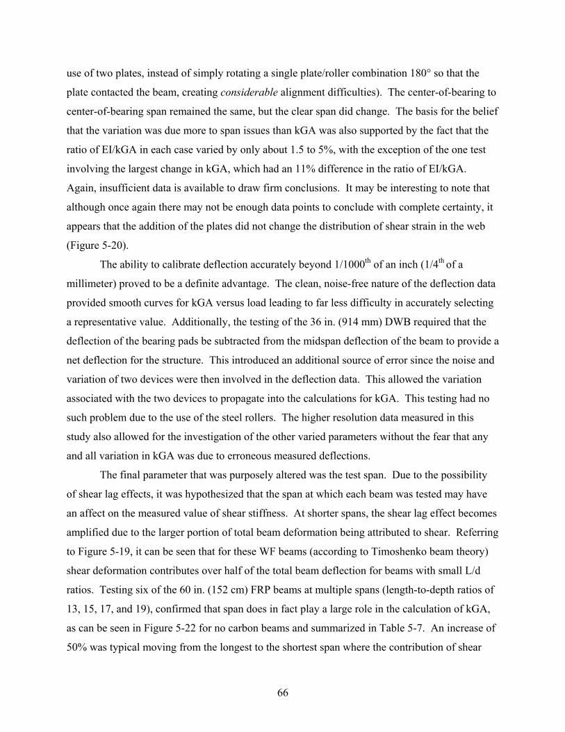
use of two plates, instead of simply rotating a single plate/roller combination 180° so that the
plate contacted the beam, creating considerable alignment difficulties). The center-of-bearing to
center-of-bearing span remained the same, but the clear span did change. The basis for the belief
that the variation was due more to span issues than kGA was also supported by the fact that the
ratio of EI/kGA in each case varied by only about 1.5 to 5%, with the exception of the one test
involving the largest change in kGA, which had an 11% difference in the ratio of EI/kGA.
Again, insufficient data is available to draw firm conclusions. It may be interesting to note that
although once again there may not be enough data points to conclude with complete certainty, it
appears that the addition of the plates did not change the distribution of shear strain in the web
(Figure 5-20).
The ability to calibrate deflection accurately beyond 1/1000th of an inch (1/4th of a
millimeter) proved to be a definite advantage. The clean, noise-free nature of the deflection data
provided smooth curves for kGA versus load leading to far less difficulty in accurately selecting
a representative value. Additionally, the testing of the 36 in. (914 mm) DWB required that the
deflection of the bearing pads be subtracted from the midspan deflection of the beam to provide a
net deflection for the structure. This introduced an additional source of error since the noise and
variation of two devices were then involved in the deflection data. This allowed the variation
associated with the two devices to propagate into the calculations for kGA. This testing had no
such problem due to the use of the steel rollers. The higher resolution data measured in this
study also allowed for the investigation of the other varied parameters without the fear that any
and all variation in kGA was due to erroneous measured deflections.
The final parameter that was purposely altered was the test span. Due to the possibility
of shear lag effects, it was hypothesized that the span at which each beam was tested may have
an affect on the measured value of shear stiffness. At shorter spans, the shear lag effect becomes
amplified due to the larger portion of total beam deformation being attributed to shear. Referring
to Figure 5-19, it can be seen that for these WF beams (according to Timoshenko beam theory)
shear deformation contributes over half of the total beam deflection for beams with small L/d
ratios. Testing six of the 60 in. (152 cm) FRP beams at multiple spans (length-to-depth ratios of
13, 15, 17, and 19), confirmed that span does in fact play a large role in the calculation of kGA,
as can be seen in Figure 5-22 for no carbon beams and summarized in Table 5-7. An increase of
50% was typical moving from the longest to the shortest span where the contribution of shear
66

deformation ranges from only 13 to 25%, respectively. Moving to shorter spans the contribution
of shear will continue to increase and amplify this shear lag effect. This may also be seen in the
overall test data (Table 5-3), as kGA as much as doubles moving from the longest to the shortest
span.
A brief summary of the variation of the aforementioned parameters and the results in
each case can be seen in Table 5-8. It seems that this study has generated as many new questions
as it has provided answers for previous ones. Firm conclusions are difficult to draw in many
cases since many factors are still unclear. One point that this testing does seem to indicate is that
the shear stiffness being measured in this type of testing of FRP beams is a structural property,
not a material property. Beam theory assumes that shear stiffness is a material property, but a
material property would not vary significantly with span or test setup as kGA does in this case.
A structural property, on the other hand, is a function of the test setup (i.e. span, loading,
boundary conditions, etc.). The shear stiffness values obtained were shown to be characteristic
of the test setup. This must be considered for the proper design and use of structural composite
beams, as the values determined for kGA are only representative under the same loading
conditions and test geometries from which they were obtained.
67

5.5 Tables and Figures
Figure 5-1. Wide flange glass FRP beam
Figure 5-2. WF beams with 0-, 1-, and 3-plies of unidirectional carbon bonded to flanges
68
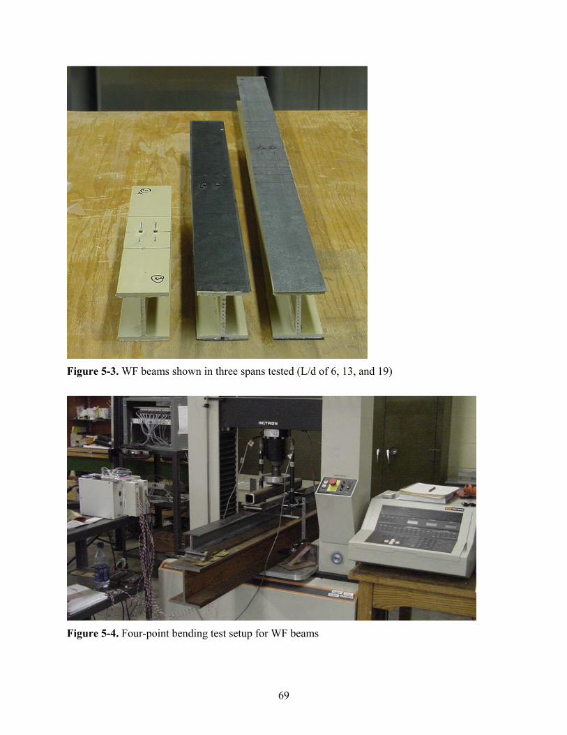
Figure 5-3. WF beams shown in three spans tested (L/d of 6, 13, and 19)
Figure 5-4. Four-point bending test setup for WF beams
69
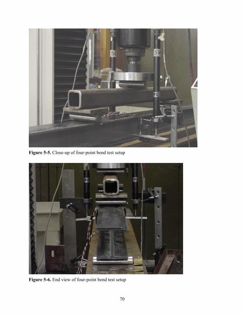
Figure 5-5. Close-up of four-point bend test setup
Figure 5-6. End view of four-point bend test setup
70
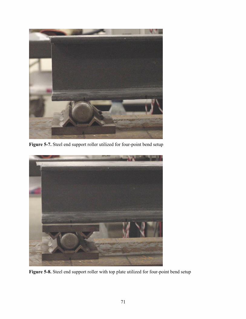
Figure 5-7. Steel end support roller utilized for four-point bend setup
Figure 5-8. Steel end support roller with top plate utilized for four-point bend setup
71
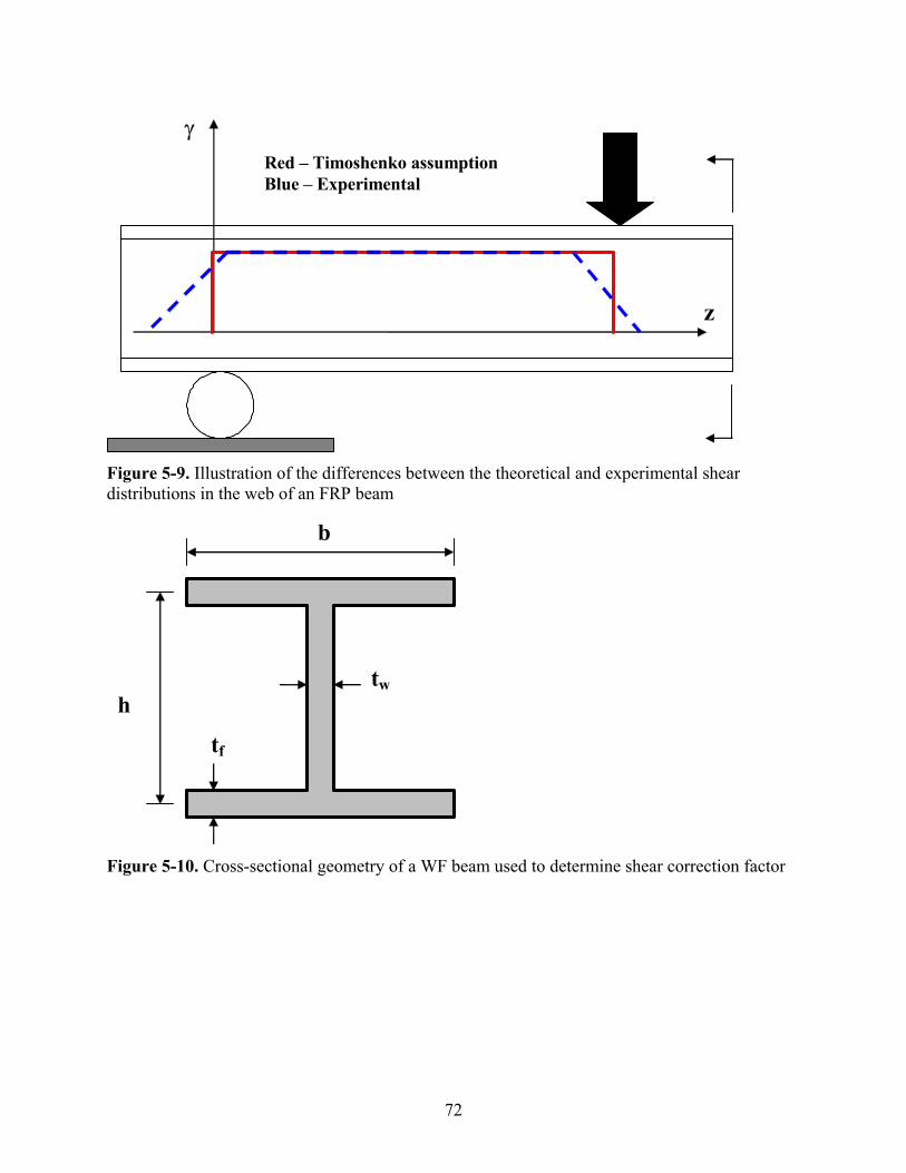
γ
z
Red – Timoshenko assumption Blue – Experimental
Figure 5-9. Illustration of the differences between the theoretical and experimental shear distributions in the web of an FRP beam b
h tw
tf
Figure 5-10. Cross-sectional geometry of a WF beam used to determine shear correction factor
72

Table 5-1. Summary of predicted values for E, G, I, and k of WF section
Msi GPa ksi GPa in4 cm4
0 Plies 3.32 22.9 605 4175 3.169 131.9 0.273 102.01-Ply 3.76 25.9 605 4175 3.249 135.2 0.278 115.4
3-Plies 4.62 31.9 605 4175 3.421 142.4 0.287 119.7
IGE EI/kGAk
0
3
6
9
0 0.1 0.2 0.3 0.4 0.5 0.6 0.7Deflection (cm)
Load
(kN
)
Figure 5-11. Typical load versus deflection plot for four-point testing of WF section
73

0
3
6
9
-2000 -1500 -1000 -500 0 500 1000 1500 2000Bending Strain (microstrain)
Load
(kN
)
Figure 5-12. Typical load versus top and bottom flange midspan bending strains
0
10
20
30
40
0 1 2 3 4 5Load (kN)
E (G
Pa)
0
5
10
15
20
kGA
(GPa
-cm
^2)
EkGA
Figure 5-13. Typical plot of bending modulus and shear stiffness versus load
74

0
10
20
30
40
0 3 6 9Load (kN)
E (G
Pa)
0
7
14
21
28
kGA
(GPa
-cm
^2)
EkGA
Figure 5-14. Plot of bending modulus and shear stiffness from 16-bit acquisition system data
0
10
20
30
40
0 2 4 6 8Load (kN)
E (G
Pa)
0
7
14
21
28
kGA
(GPa
-cm
^2)
EkGA
Figure 5-15. Same beam as shown in Figure 5-14 tested using 12-bit acquisition system
75

Table 5-2. Summary of average E and kGA for each span for WF beam testing. Note that the case where the Coefficient of Variation is zero occurred when the two beams tested had identical calculated values for kGA.
C.O.V. C.O.V.Msi GPa % ksi-in² GPa-cm² %
6 0 4.13 28.48 3.31 346 15.4 1.26 37.8113 0 4.07 28.06 0.51 260 11.6 1.02 49.6519 0 4.09 28.20 1.22 176 7.8 4.26 73.6213 1 4.45 30.68 3.02 308 13.7 0 46.8919 1 4.36 30.06 - 232 10.3 - 61.076 3 5.18 35.72 1.58 371 16.5 11.99 42.9613 3 4.99 34.41 1.50 350 15.6 2.33 48.8019 3 5.06 34.89 1.82 239 10.6 3.55 72.43
Eavg EI/kGAL/d C-Plies kGAavg
Table 5-3. Individual beam results for E and kGA
C Plies L/d E (Msi) E (GPa) kGA (ksi-in2) kGA (GPa-cm²) EI/kGA0 6 4.22 29.1 341 15.2 39.220 6 4.19 28.9 349 15.5 38.050 6 3.97 27.4 348 15.5 36.163 6 5.16 35.6 421 18.7 38.843 6 5.27 36.3 358 15.9 46.653 6 5.11 35.2 335 14.9 48.340 13 4.09 28.2 263 11.7 49.290 13 4.08 28.1 258 11.5 50.120 13 4.05 27.9 259 11.5 49.561 13 4.54 31.3 308 13.7 46.721 13 4.35 30.0 308 13.7 44.763 13 5.06 34.9 359 16.0 44.673 13 4.91 33.9 344 15.3 45.243 13 4.99 34.4 346 15.4 45.710 19 4.04 27.9 184 8.2 69.590 19 4.09 28.2 176 7.8 73.650 19 4.14 28.5 169 7.5 77.641 19 4.36 30.1 232 10.3 59.563 19 5.12 35.3 233 10.4 69.643 19 4.99 34.4 245 10.9 64.55
76

0
20
40
60
80
5 7 9 11 13 15 17 19L/d
EI/k
GA No Carbon
1-Ply3-Plies
Figure 5-16. Ratio of EI/kGA versus span for all three beam types
6
12
18
24
5 7 9 11 13 15 17 19L/d
kGA
(GPa
-cm
^2)
No Carbon1-Ply3-Plies
Figure 5-17. Average kGA for each beam type versus span
77

Table 5-4. Summary of results for shear modulus determined by back calculating G from kGA
ksi-in² GPa-cm² in² cm² ksi GPa6 0 346 15.4 0.27284 0.750 4.84 1691 11.66
13 0 260 11.6 0.27284 0.750 4.84 1271 8.7619 0 176 7.8 0.27284 0.750 4.84 862 5.9413 1 308 13.7 0.2781 0.754 4.86 1470 10.1319 1 232 10.3 0.2781 0.754 4.86 1107 7.636 3 371 16.5 0.28678 0.886 5.72 1461 10.08
13 3 350 15.6 0.28678 0.886 5.72 1376 9.4919 3 239 10.6 0.28678 0.886 5.72 941 6.49
L/d kGA AV GC-Plies k
-700
-600
-500
-400
-300
-200
-100
0
100
0 10 20 30 40 50 60 70
Distance from beam end (cm)
Shea
r Str
ain
(mic
rost
rain
)
No Carbon (1 kip)3-Plies (1 kip)
Figure 5-18. Distribution of shear strain in beam web for no plies and 3-plies of carbon lamina
78

0
10
20
30
40
50
60
70
6 13L/d
% S
hear
def
lect
ion
20
No Carbon1-Ply3-Plies
E (GPa) kGA (GPa-cm²) EI/kGA0 Plies 28.3 11.6 50.001 Ply 30.4 11.8 53.843 Plies 35.0 14.4 53.86
Figure 5-19. Contribution of shear deformation to the total beam deflection at test spans, calculated using the average bending modulus and shear stiffness for each beam
-700
-600
-500
-400
-300
-200
-100
0
100
200
0 10 20 30 40 50 60 70
Distance from beam end (cm)
Stra
in (m
icro
stra
in)
1 kip with plates1 kip no plates
Figure 5-20. Distribution of shear strain in beam web for point load and load patch cases
79
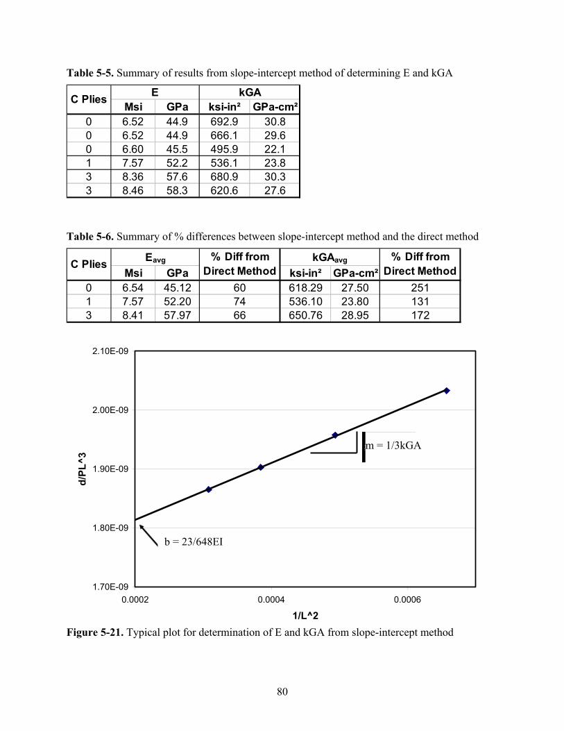
Table 5-5. Summary of results from slope-intercept method of determining E and kGA
Msi GPa ksi-in² GPa-cm²0 6.52 44.9 692.9 30.80 6.52 44.9 666.1 29.60 6.60 45.5 495.9 22.11 7.57 52.2 536.1 23.83 8.36 57.6 680.9 30.33 8.46 58.3 620.6 27.6
C Plies E kGA
Table 5-6. Summary of % differences between slope-intercept method and the direct method
Msi GPa ksi-in² GPa-cm²0 6.54 45.12 60 618.29 27.50 2511 7.57 52.20 74 536.10 23.80 1313 8.41 57.97 66 650.76 28.95 172
C Plies Eavg kGAavg% Diff from Direct Method
% Diff from Direct Method
1.70E-09
1.80E-09
1.90E-09
2.00E-09
2.10E-09
0.0002 0.0004 0.0006
1/L^2
d/PL
^3
m = 1/3kGA
b = 23/648EI
Figure 5-21. Typical plot for determination of E and kGA from slope-intercept method
80
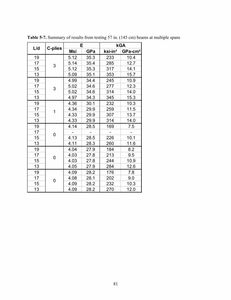
Table 5-7. Summary of results from testing 57 in. (145 cm) beams at multiple spans
Msi GPa ksi-in² GPa-cm²19 5.12 35.3 233 10.417 5.14 35.4 285 12.715 5.12 35.3 317 14.113 5.09 35.1 353 15.719 4.99 34.4 245 10.917 5.02 34.6 277 12.315 5.02 34.6 314 14.013 4.97 34.3 345 15.319 4.36 30.1 232 10.317 4.34 29.9 259 11.515 4.33 29.9 307 13.713 4.33 29.9 314 14.019 4.14 28.5 169 7.517 - - - -15 4.13 28.5 226 10.113 4.11 28.3 260 11.619 4.04 27.9 184 8.217 4.03 27.8 213 9.515 4.03 27.8 244 10.913 4.05 27.9 284 12.619 4.09 28.2 176 7.817 4.08 28.1 202 9.015 4.09 28.2 232 10.313 4.09 28.2 270 12.0
3
3
0
0
0
1
kGAEC-pliesL/d
81

0
5
10
15
12 14 16 18 20L/d
kGA
(GPa
-cm
^2)
No plies 1No plies 2No plies 3
Figure 5-22. Span dependence of shear stiffness for beams with no carbon plies
82

Table 5-8. Summary of parameters varied, the method of variation, and results from testing of WF FRP sections
Varied Parameter Method of Variation Results and Comments
EI/kGA Addition of carbon plies. 7 to 26% increase in kGA, but k and A contribute 80% of that.
16-bit acquisition system andLVDT used for measurements
60 in. (152 cm) beams weretested at multiple spans. Andthree spans were used overall.
Multi-Span Method was used.
Steel plates at load/supportsBoundary Conditions
Test Span
Deflection
Test Method
Significant affect on kGA. 50% increases for L/d changes of 6. 100% or more increases were not uncommon going from longest to shortest span.
Test to test variation in kGA was typically well below 1%. Data was clean and noise-free leading to confidence in kGA calcualtions.
Multi-span results were drastically different, attributed to test method, not kGA.
Typically less than 10% change in kGA. EI/kGA changed very little (1.5 to 5%, one 11% change). No significant affect on distribution of shear strain in web (limited test data).
83
Chapter 6 Conclusions and Recommendations
Based upon the investigations performed during the research and writing of this thesis,
the following conclusions and recommendations are made:
By means of the low load stiffness testing of nineteen 36 in. DWBs, the values for
bending modulus (E) and shear stiffness (kGA) were determined that will be included in
the structural design guide for this girder.
Through the failure testing of the same nineteen 36 in. DWBs, the ultimate load limits
were determined for the structural design guide. In addition to this, the failure modes of
the structure were determined. It was found that there is more than one factor controlling
design utilizing this structure, i.e. the shear capacity of the structure seems to dominate
the failure mode until a span limit is reach (somewhere between an L/d of 6 and 10), at
which bearing failures occur due to the concentration of stresses created by the
elastomeric bearing pads.
The A and B allowables for E, kGA, shear capacity, and moment capacity were
determined in order to provide future users of the design guide with material properties
that will lead to safely and efficiently designed structures.
A great deal of variation can be seen in the experimentally determined value of shear
stiffness (kGA) for the 36 in. DWB. Inaccurate and high-noise deflection data is believed
to be one of the primary sources of the variation as it has been seen that kGA is extremely
sensitive to measured deflections. It was determined that it was essential to use
deflection data measured using a highly sensitive device, such as the LVDT used in this
research. The use of higher resolution acquisition systems proved to be an important
aspect of testing as well. The use of an acquisition system with 16-bit resolution
combined with a deflection measuring device with a longer stroke would be ideal as it
appears that kGA tends to level off as load increases
84
In order to further examine shear effects in FRP beams, the small WF beam testing
described in Chapter 5 was conducted. This study revealed that it is possible to
consistently obtain values for shear stiffness as test to test variation was minimal and
beam to beam variations were reasonable. It also revealed that all the factors thought to
affect kGA or the ability to measure it do indeed have affects. Structure stiffness,
boundary conditions, span, and deflection data all proved to have considerable affects on
the measurement of kGA. The slope-intercept method for determining kGA proved to be
ineffective for unexplained reasons.
Predictions made during the WF beam study proved to be on the conservative side. This
may in part be due to the difficulty had in turning a thread-up into an accurate and
representative lay-up to be used in CLT and MLB theory.
The study conducted on the WF beams also seemed to raise as many, if not more,
questions regarding the characterization of shear effects in FRP structures as it answered.
What is the true length required before shear strain in the web levels off to a constant
value around the load points? What are the effects of shear lag in FRP structures?
Exactly how much does span and the increased contribution of shear deformation at short
spans play a role in the value of kGA? How necessary is a more complex beam theory to
better account for the shear deformation in FRP structures? What measured kGA is the
true property? Etc.
Although the WF beam study introduced a number of questions, it seems to have at least
suggested a path and pointed researchers in the direction of better understanding shear
effects. It is a foundation upon which to build.
And finally, the kGA being measured in these experiments was shown to be a structural
property, characteristic of the test setup from which it was obtained. That said, care must
be taken to ensure proper use of kGA in design using these structures. The values
presented for shear stiffness, kGA, are specific to the test setups/conditions described
herein.
85
References 1. Hayes, M.D., Lesko, J.J, Weyers, R.E., Cousins, T.E., Haramis, J., Gomez, J. and Masarelli,
P. 2000. “Laboratory and Field Characterization of the Tom’s Creek Bridge Superstructure,” Journal for Composites in Construction, 4(3): 120-128.
2. Strongwell. 2000. “EXTREN DWB™ Design Guide” 3. AASHTO (1998), LRFD Bridge Design Specification, 2nd edition, American Association of
State Highway and Transportation Officials, Washington, D.C. 4. GangaRao, H.V.S., H.K. Thippeswamy, V. Shekar, C. Craigo, “Development of Glass Fiber
Reinforced Polymer Composite Bridge Deck,” SAMPE Journal, Vol. 35, No. 4, July/August 1999.
5. Brailsford, B., S.M. Milkovich, D.W. Prine, J.M. Fildes, "Definition of Infrastructure Specific Markets for Composite Materials: Topical Report," Northwestern University BIRL Project P93-121/A573, July 11, 1995.
6. Hayes, M.D., “Characterization and Modeling of a Fiber-Reinforced Polymeric Composite Structural Beam and Bridge Structure for Use in the Tom’s Creek Bridge Rehabilitation Project,” Master’s Thesis, Virginia Polytechnic Institute and State University, 1998.
7. Hargrave, M.W., E. Munley, and T.J. Pasko, "FHWA's applied highway infrastructure research program on composite materials," Public Roads, v60 n4 (Spring 1997), 23 (9).
8. Lesko, J.J., S.W. Case, T.E. Cousins, “Design Manual Development for FRP Structural Shapes: Practical and Durability Considerations,” International SAMPE Symposium and Exhibition, v.46 II 2001:1576-1586.
9. Strongwell. 1989. “EXTREN™ Design Guide” 10. Hardcore Composites Website: www.hardcorecomposites.com 11. Creative Pultrusions Website: www.creativepultrusions.com 12. Machida, A. ed., “Recommendation for Design and Construction of Concrete Structures
Using Continuous Fiber Reinforcing Materials,” Japan Society of Civil Engineers, 1997. 13. American Concrete Institute, “Guide for the Design and Construction of Concrete Reinforced
with FRP Bars,” ACI Committee 440, Revised January 17, 2000. 14. Zenkurt, D., An Introduction to Sandwich Construction, Engineering Materials Advisory
Services LTD., 1995: 50-61. 15. Omidvar, B., “Shear Coefficient in Orthotropic Thin-Walled Composite Beams,” Journal of
Composites for Construction, February 1998. 16. Cowper, G.R., “The shear Coefficient in Timoshenko’s Beam Theory”, Journal of Applied
Mechanics, June 1966: 335-340. 17. Bank, L.C., “Shear Coefficients for Thin-Walled Composite Beams,” Composite Structures,
1987. 18. Whitney, J.M., “Shear Correction Factors for Orthotropic Laminates Under Static Load,”
Journal of Applied Mechanics, 1973, 40(3), 302-304. 19. Madabhusi-Raman, P., J. Davalos, “Static shear Correction Factor for Laminated
Rectangular Beams,” Composites. Part B, 27(3-4), 285-293. 20. Bank, L.C., “Flexural and Shear Moduli of Full-Section Fiber Reinforced Plastic Beams,”
ASTM, 1989. 21. Pai, P.F., M.J. Schulz, “Shear Correction Factors and an Energy-Consistent Beam Theory,”
Intl. J. of Solids and Structures, 36, 1999: 1523-1540.
86

22. Barbero, E.J., R. Lopez-Anido, J.F. Davalos, “On the Mechanics of Thin-Walled Laminated Composite Beams,” J. of Composite Materials, Vol. 27, No. 8, 1993.
23. Waldron, C.J., “Determination of the Design Parameters for the Route 601 Bridge,” Master’s Thesis, Virginia Polytechnic Institute and State University, 2001.
24. Dufort, L., M. Grediac, Y. Surrel, “Experimental Evidence of the Cross-Section Warping in Short Composite Beams Under Three Point Bending,” Composite Structures, 51, 2001: 37-47.
25. Weibull, Waloddi (1951), “A Statistical Distribution Function of Wide Applicability,” J. of Applied Mechanics, 293-297.
26. Weibull, Waloddi (1949), “A Statistical Representation of Fatigue Failures in Solids, Transitions of the Royal Institute of Technology”, No. 27, Stockholm.
27. Mil-17 Organization, “The Composite Materials Handbook”, www.mil17.org.
87

Appendices
Appendix A
The basis for the calculations in the design guide comes from Weibull statistics, where the
cumulative probability distribution function that describes the distribution of experimental values
is derived from,
F(x) = 1 – Exp[-(x/β)α] (Α−1)
where α and β are parameters used to fit the data. Alpha is the shape parameter, which describes
the breadth of the distribution. Beta is the location parameter, which defines the value nearest
the center of the distribution. The probability of failure, F(x), is related to the reliability, R(x),
by,
R(x) = 1 – F(x) (A-2)
This relationship can then be arranged to obtain expressions for A and B basis allowables, as
seen below in Equations (A-5) and (A-6). Further details on Weibull statistics and the equations
seen below can be found in the EXTREN DWB Design Guide [2], Weibull [25, 26], and from
the Mil-17 Specification “The Composite Materials Handbook” [27].
• Mean:
+
Γ⋅=α
αβµ 1 (A-3)
where Γ is the gamma function. • Standard deviation:
2
1
12
+
Γ
Γ
αα22
−
+⋅=
ααβσ (A-4)
• A allowable:
α
β1
99.01ln~
lower (A-5)
• B allowable:
88

α
β1
90.01ln~
upper (A-6)
where α
ββ1
05.02
2~
Χ=
nlower ,
αββ
1
95.02
2~
Χ=
nupper (A-7)
• Weibull density function:
−
=
− αα
βββα xxxf exp)(
1
(A-8)
• Weibull cumulative distribution: α
β∫∞
−−==
0
exp1)()( xdxxfxF (A-9)
• reliability:
−=
α
β~1exp xR
where x is the allowable design value (A-10)
89

Appendix B
*All values are in English units (E—Msi, kGa—Msi-in²) Beam Span test Load E (600-800) kGA (600-800) E (min-600) kGA (min-600)
30 footer 30 failure test 250 6.70 47.3 6.76 44.67/12-2a 30 test 11 250 6.44 43.2 6.45 42.3
8 150 6.41 41.5 6.42 41.77 80 6.37 40.5 6.39 40.76 80 6.47 46.2 6.47 44.95 60 6.49 45.4
7/12-2b 30 failure test 260 6.28 50.8 6.32 48.17 100 6.41 51.6 6.41 49.56 80 6.41 46.5 6.41 46.45 80 6.41 47.4 6.41 47.3
7/10-#5 30 8 100 6.63 49.7 6.65 47.77 100 6.62 50.4 6.64 48.16 80 6.63 50.4 6.64 48.75 80 6.63 50.8 6.64 48.7
7/12-#3 30 8 100 6.52 64.3 6.53 58.47 80 6.53 60.7 6.53 56.36 80 6.52 62.1 6.53 57.8
7/11-#1 39 4 40 6.27 44.55 40 6.26 44.4 6.28 43.2
7/12-#1 39 3 40 6.18 49.0 6.20 47.14 40 6.22 52.3 6.22 50.35 40 6.24 53.5 6.24 50.7
7/9-#2 39 8 40 6.01 53.9 6.03 53.79 40 6.04 60.6 6.04 58.110 40 6.00 61.1 6.00 58.5
7/9-#1 39 3 (LVDT) 40 6.50 39.2 6.50 38.04 (LVDT) 40 6.46 41.6 6.46 39.85 (LVDT) 40 6.51 39.4 6.50 38.13 (WP) 40 6.50 60.4 6.50 52.89 (WP) 100 6.48 46.8 6.48 45.8
#14 39 3 40 6.62 39.9 6.62 38.85 40 6.61 40.4 6.62 39.2
failure (WP) 230 6.61 38.3 6.60 38.1#24 39 3 40 6.28 46.6 6.28 44.6
4 40 6.28 45.8 6.28 44.25/31-#1 58 15 20 6.40 53.55/31-#3 58 2 20 6.67 52.0 6.66 42.5
3 20 6.64 52.5 6.71 43.65/29-#1 58 3 20 6.44 36.6
4 20 6.46 39.47/11-#1 58 3 20 6.37 41.27/11-#2 58 3 20 6.37 41.3
5 20 6.40 46.5
90

Appendix C
All values are in English units (E—psi, kGA—psi-in²) beam test E (avg) Emin Emax St Dev kGA (avg) kGA min kGA max St Dev20(0)-2A test 2 4.24E+06 4.22E+06 4.26E+06 1.21E+04 3.32E+05 3.04E+05 3.60E+05 1.93E+04
test 3 4.19E+06 4.18E+06 4.21E+06 1.16E+04 3.51E+05 3.23E+05 3.79E+05 1.93E+0420(0)-3A test 3 4.19E+06 4.18E+06 4.21E+06 1.16E+04 3.51E+05 3.23E+05 3.79E+05 1.93E+04
test 4 4.19E+06 4.17E+06 4.20E+06 1.17E+04 3.47E+05 3.18E+05 3.76E+05 1.98E+0420(0)-G test 1 3.95E+06 3.95E+06 3.96E+06 3.43E+03 3.51E+05 3.41E+05 3.59E+05 6.17E+03
test 3 3.98E+06 3.97E+06 3.98E+06 1.74E+03 3.45E+05 3.35E+05 3.55E+05 6.90E+0320(3)-1A test 2 5.16E+06 5.15E+06 5.17E+06 9.04E+03 4.22E+05 4.05E+05 4.39E+05 1.20E+04
test 3 5.15E+06 5.14E+06 5.16E+06 8.15E+03 4.20E+05 4.04E+05 4.36E+05 1.14E+0420(3)-2A test 1 5.28E+06 5.27E+06 5.28E+06 1.99E+03 3.58E+05 3.32E+05 3.84E+05 1.78E+04
test 2 5.27E+06 5.27E+06 5.27E+06 1.73E+03 3.58E+05 3.31E+05 3.86E+05 1.94E+0420(3)-G test 2 5.05E+06 5.03E+06 5.06E+06 1.23E+04 3.42E+05 3.23E+05 3.61E+05 1.28E+04
test 1 5.17E+06 5.12E+06 5.18E+06 2.23E+04 3.29E+05 3.12E+05 3.45E+05 1.11E+0440(0)-1A test 1 4.08E+06 4.08E+06 4.09E+06 2.41E+03 2.62E+05 2.49E+05 2.75E+05 8.56E+03
test 2 4.09E+06 4.08E+06 4.10E+06 4.55E+03 2.65E+05 2.53E+05 2.79E+05 8.87E+0340(0)-2A test 1 4.08E+06 4.06E+06 4.10E+06 1.69E+04 2.58E+05 2.48E+05 2.68E+05 6.44E+0340(0)-G test 2 4.04E+06 4.03E+06 4.05E+06 4.65E+03 2.58E+05 2.56E+05 2.59E+05 9.48E+02
test 3 4.05E+06 4.04E+06 4.06E+06 6.57E+03 2.61E+05 2.60E+05 2.62E+05 5.77E+0240(1)-2A test 1 4.53E+06 4.50E+06 4.57E+06 2.39E+04 3.10E+05 3.09E+05 3.11E+05 5.75E+02
test 2 4.55E+06 4.52E+06 4.58E+06 2.03E+04 3.07E+05 3.05E+05 3.08E+05 8.80E+0240(1)-3A test 1 4.34E+06 4.34E+06 4.35E+06 4.02E+03 3.09E+05 3.00E+05 3.19E+05 6.02E+03
test 2 4.35E+06 4.34E+06 4.36E+06 4.51E+03 3.08E+05 2.97E+05 3.18E+05 7.11E+0340(3)-1A test 1 5.06E+06 5.04E+06 5.07E+06 8.08E+03 3.53E+05 3.43E+05 3.64E+05 7.02E+03
test 2 5.07E+06 5.05E+06 5.08E+06 7.57E+03 3.65E+05 3.57E+05 3.73E+05 5.19E+0340(3)-3A test 1 4.92E+06 4.91E+06 4.94E+06 9.28E+03 3.30E+05 3.07E+05 3.56E+05 1.64E+04
test 2 4.90E+06 4.90E+06 4.91E+06 2.12E+03 3.58E+05 3.41E+05 3.78E+05 1.26E+0440(3)-G test 4 4.98E+06 4.96E+06 4.99E+06 1.04E+04 3.44E+05 3.39E+05 3.51E+05 3.85E+03
test 5 5.01E+06 4.98E+06 5.02E+06 1.32E+04 3.47E+05 3.39E+05 3.56E+05 5.50E+0360(0)-2A test 1 4.03E+06 4.03E+06 4.04E+06 3.96E+03 1.84E+05 1.79E+05 1.89E+05 3.26E+03
test 2 4.04E+06 4.03E+06 4.05E+06 5.95E+03 1.84E+05 1.79E+05 1.89E+05 3.32E+0360(0)-3A test 1 4.09E+06 4.08E+06 4.10E+06 7.09E+03 1.75E+05 1.70E+05 1.80E+05 3.28E+03
test 2 4.10E+06 4.08E+06 4.11E+06 9.89E+03 1.76E+05 1.72E+05 1.81E+05 3.09E+0360(0)-G test 1 4.13E+06 4.11E+06 4.14E+06 7.47E+03 1.68E+05 1.67E+05 1.68E+05 4.47E+02
test 2 4.15E+06 4.13E+06 4.17E+06 1.21E+04 1.71E+05 1.70E+05 1.72E+05 4.08E+0260(1)-3A test 1 4.37E+06 4.35E+06 4.38E+06 8.63E+03 2.31E+05 2.27E+05 2.34E+05 2.30E+03
test 2 4.35E+06 4.34E+06 4.37E+06 1.06E+04 2.34E+05 2.33E+05 2.36E+05 9.48E+0260(3)-1A test 1 5.12E+06 5.11E+06 5.12E+06 7.02E+03 2.31E+05 2.22E+05 2.41E+05 6.17E+03
test 2 5.13E+06 5.11E+06 5.14E+06 9.86E+03 2.36E+05 2.26E+05 2.45E+05 6.52E+0360(3)-2A test 1 4.99E+06 4.99E+06 5.00E+06 1.61E+03 2.44E+05 2.38E+05 2.50E+05 3.98E+03
test 2 4.99E+06 4.98E+06 4.99E+06 3.74E+03 2.46E+05 2.39E+05 2.52E+05 3.84E+03
91

Appendix D – Typical Failure Pictures for the 36 in. DWB
92

93

94
Vita
Timothy J. Schniepp was born in Rochester, Minnesota on January 17, 1978 to Becky
and Brian Schniepp. He grew up in the town of Elgin, Minnesota in Southeastern Minnesota.
Tim graduated from Elgin-Millville High School as valedictorian in 1996 and then proceeded to
attend Winona State University in Winona, MN. Tim graduated from WSU in May 2000 with a
B.S. in Composite Materials Engineering and then made the decision to continue his education at
Virginia Tech. While working to fulfill the requirements for his M.S. in Engineering Science
and Mechanics at VT, Tim studied various aspects of fiber-reinforced composite materials and
their use in civil infrastructure applications. Upon completion of his M.S. in August 2002, Tim
has accepted a position working for Lockheed Martin Aeronautics Company in Marietta,
Georgia where he will be a member of the Composites and Adhesives division of the Materials,
Processes, and Producibility department.