design, implementation, calibration and validation of...

UNIVERSITY OF ALMERIA

Automatic Control, Electronics and Robotics Research Group

Technical Report

DESIGN, IMPLEMENTATION, CALIBRATION AND VALIDATION OF A DYNAMIC MODEL OF GREENHOUSE CLIMATE BASED ON PHYSICAL

PRINCIPLES

Francisco Rodríguez Díaz Manuel Bereguel Soria

Almería (SPAIN)

November 2002

42

DESIGN, IMPLEMENTATION, CALIBRATION AND VALIDATION OF A DYNAMIC MODEL OF GREENHOUSE CLIMATE BASED ON PHYSICAL

PRINCIPLES

F. Rodríguez*, M. Berenguel*

*Universidad de Almería. Dpto. Lenguajes y Computación. Ctra. Sacramento s/n, La Cañada, E04120, Almería, Spain. Fax: ++34 950 015129. E-mail: [email protected], [email protected]

Abstract: This paper presents the steps followed to obtain a model of greenhouse climate. This model is of capital interest in the study of the dynamics of the greenhouse crop production process under different control policies, aimed at achieving adequate inside climate conditions to avoid extreme situations and to optimise crop production while reducing pollution and energy consumption. Several models of greenhouse climate based on physical principles have been developed in different areas, neither of them showing the complete methodology used for developing the model. This paper presents a hierarchical and modular procedure to design, implement, calibrate and validate a greenhouse climate model based on physical principles. Illustrative results comparing the real measured data and data estimated by the model for South Spain greenhouses are also provided, to show the ability of the model to simulate the real inside climate of industrial greenhouses. Keywords: Greenhouse climate modeling, Physical models, Computer simulation.

1. INTRODUCTION The development of greenhouse climate models required for decision support within the framework of crop production processes has been impelled by the massive use of the computer as a simulation tool. The main advantages of these models are that they allow the evaluation of the evolution of a real world decision system without having to wait for the real system to produce such results (usually in a time scale much longer than that achieved with the simulation model). These models also allow the organization of the knowledge and the observations on the system, provide a framework to verify the system and its possible modifications and a perspective on details and the main aspects of the system, help to manipulate and control the main variation sources and disturbances acting on the system, facilitate the analysis of the results and the realization of different experiences, as these are cheaper than those performed on the real system. The dynamic behavior of the microclimate inside the greenhouse is a combination of physical processes involving energy transfer (radiation and heat) and mass balance (water vapor fluxes and CO2 concentration). These processes depend on the outside environmental conditions, structure of the greenhouse, type and state of the crop and on the effect of the control actuators (typically ventilation and heating to modify inside temperature and humidity conditions, shading and artificial light to change internal radiation, CO2 injection to influence photosynthesis and fogging/cooling for humidity enrichment). The development of models of a dynamic system is a complex process, that depends on the characteristics of the dynamics of the process object of study. As pointed out by Pearson, when a complex system is modeled, one of the questions that arises is to discern if models based on first principles or empirical models based on the experimental data are used (Pearson 1995). The first ones generally provide a more detailed information of the process than the empirical models, but they are usually more complex requiring longer times in the design phase. Although the models based on first principles can be used within model based control structures, they are usually used for simulation purposes while the empirical models are used for control tasks. These two approaches can be found within the framework of the greenhouse climate variables modeling. This paper deals with models based on physical principles, as this is not a completely solved problem. These models have been developed in different zones of the world from the Sixties, applied to several greenhouse structures (main of them of

42

low size for research purposes), with different climatic actuators, cover material and crops. Among them, it is interesting to emphasize several works related to that presented in this paper:

North and Central Europe: Bot (1983), Udink ten Cate (1983), Halleaux (1989), Young et al. (1993), van Henten (1994), Tchamitchan et al. (1993, 1996), Tap et al. (1996a, 1996b, 2000).

Mediterranean area: Kindelan (1980), Cormary and Nicolas (1983), Chaabane (1986), Manera et al. (1990), Boisson (1991), Ioslovich el al. (1995), Zhang et al. (1997), Senent et al. (1998), Wang and Boulard (2000), and Tavares et al. (2001).

North America: Takakura el al. (1971, 1993), Ahmadi et al. (1982a, 1982b,1984), Halleaux (1989), Trigui et al. (2001a, 2001b)

South of Asia: Sharme et al.(1999).

Although all these models are based on the same physical principles, they are different because some aspects are modified in order to adapt them to the particular conditions in each area. All these works describe some of the equations of the mathematical models and show some results, but they do not show the complete methodology used for the implementation, calibration and validation of the models. In the case treated in this paper, a complex nonlinear dynamical model of the greenhouse climate has been developed for the particular conditions of the Southeast of Spain, where the largest concentration of greenhouses in the world is located (Rodríguez, 2002). These greenhouses are characterized by low-cost structures of medium yield, normally passive or with a low-level of automation and made of plastic cover, taking advantage of favorable outside climatic conditions. In section 2, a description of the dynamic model of the industrial greenhouse climate is formulated. It is composed of six submodels describing the cover temperature, the soil surface temperature, the first soil layer temperature, the inside air temperature and humidity and the PAR (Photo-synthetically active radiation) radiation onto the canopy. Section 3 is devoted to explain the industrial greenhouse structures modeled in the paper and the equipment necessary to calibrate and validate the models. Next, in section 4, the model implementation is described. It has been hierarchically implemented, by using top-down and bottom-up approaches to provide insight into how the model is organized and how its parts interact. Two different modeling paradigms, block-oriented modeling and object-oriented modeling, have been used. For the first modeling approach, the Simulink (Mathworks Inc., 1998a, 1998b) software package has been used. The second modeling approach has been tackled using the object-oriented and equation-based declarative modeling language Modelica (Dynasim, 2003a, 2003b). Section 5 shows the methodology proposed to estimate the unknown parameters of the model based on the fact that the involved physical processes are not coupled. A combination of sequential iterative search and genetic algorithms techniques have been used to search the values of the parameters of the model obtaining acceptable results. A sensitivity analysis of the model with respect to the parameters is included in section 6. Section 7 shows the model validation process with different greenhouse structures in winter, spring and summer seasons, comparing real data measured in greenhouses with data estimated by the model. Finally, section 8 presents some conclusions of the work putting special emphasis on the generality of the proposed technique to develop a composed model of the greenhouse climate in any location of the world with its own characteristics. The main possible applications of the model are also commented. 2. DYNAMIC MODELING OF GREENHOUSE CLIMATE 2.1 General hypotheses The greenhouse climate can be described by a dynamic model represented by a system of differential equations given by:

),,,,,(

CVDUXfd

dX with ii X)(X (1)

X=X() is a n-dimensional vector of state variables, U=U() is a m-dimensional vector of input variables, D=D() is an o-dimensional vector of disturbances, V=V() is a p-dimensional vector of system variables, C

42

is a q-dimensional vector of system constants, is the time, Xi is the known initial state at the initial time i and f=f() is a non-linear function based on mass and heat transfer balances. The number of equations describing the system and their characteristics depend on the greenhouse elements, the installed control actuators and the type of cultivation method. The model presented in this paper corresponds to a typical industrial greenhouse located at the Mediterranean area with a tomato crop. It has been developed assuming some general hypotheses: The greenhouse is divided into four elements: cover, internal air, soil surface and one soil layer. The crop

is not considered as an element as no measurements of the leaf temperature are actually available and thus it is considered as a source of disturbances for the inside climate. As some of the physical processes require the crop temperature to be known (i.e. thermal radiation among the solid elements), it has been considered to be equal to the greenhouse air temperature.

The state variables of the model are1 the internal air temperature (Xt,a) and humidity (absolute Xha,a and relative Xhr,a), cover temperature (Xt,cv), soil surface temperature (Xt,ss) and first soil layer temperature (Xt,s1). The PAR radiation onto the canopy (output variable Xrp,,a) is also modeled with an algebraic equation. The CO2 concentration is not considered (although is one of the main variables affecting the crop growth) because nowadays its control is very expensive in the South of Spain, so measurements of this variable are no acquired. In any case, as will be shown later, its inclusion in the model is very easy due to the modular and hierarchical methodology used in the design.

The exogenous and disturbance inputs acting on the system are the outside air temperature (Dt,e) and absolute humidity (Dha,e), wind speed (Dws,e) and direction (Dwd,e), sky temperature (Dt,sky), calculated using the Swinbank formula (Boisson, 1991), outside global solar radiation (Drs,e), PAR radiation (Drp,e), greenhouse whitening (Dwh), the transpiration rate inside the greenhouse via the leaf area index (DLAI) and the temperature of the deepest soil layer (Dt,s2) which can be calculated as the average of the external air temperature during one year or measured using dedicated sensors.

The control inputs of the system are the position of the natural ventilation (Uven), the position of the shade screen (Ushd) and the water temperature of the pipe heating system (Ut,heat).

The heat fluxes are one-dimensional. The model only considers the vertical dimension. The temperature models are based on a heat transfer balance where the following physical processes are

included: solar (sol) and thermal radiation (rad) absorption, heat convection (cnv) and conduction (cnd), crop transpiration (trp), condensation (cd) and evaporation (evp).

In order to design the humidity model, a mass balance has been used based on the artificial water influxes, exchange with the outside, crop, condensation and evaporation.

The models of short and long wave radiation do not consider the reflection, and the air is inert to theses processes.

The physical characteristics of the different elements (cover material, soil components, air, etc.), such as density or specific heat are considered constant.

In what follows, the models needed to perform the heat transfer and mass balances in the four elements constituting the greenhouse are developed. 2.2 Model of the PAR radiation

The PAR radiation onto the canopy is modeled using an algebraic equation, because it is similar to the PAR radiation outside the greenhouse dimmed by the different physical elements that absorb the radiation (mainly

cover material, cover whitening and shade screen). So it is modeled using the following equation:

e,rpg,tswa,rp DVX (2)

where Vtsw,g is the greenhouse short wave radiation transmission coefficient, described by:

1 The units and notation followed through the text is described in Appendix A.

42

whiteningshadeCCC

whiteningnoshadeCC

whiteningshadenoCC

whiteningnoshadenoC

V

shdtswwhtswcvtsw

shdtswcvtsw

whtswcvtsw

cvtsw

gtsw

,

,

,

,

,,,

,,

.,

,

,

(3)

Where Ctsw,cv is the cover solar transmission coefficient, Ctsw,shd is the shade screen solar transmission coefficient and Ctsw,wh is the whitening solar transmission. This last parameter is difficult to determine because it depends of the whiting concentration between 4 Kg whiting/4 l water (Ctsw,wh= 0.1) and 0.7 Kg whiting/ 4 l water (Ctsw,wh= 0.65) (Montero, 1998). It is thus necessary to take measurements of global and PAR radiation inside and outside the greenhouse to determine this coefficient. Another option is to search the value of this parameter in the calibration phase. 2.3 Heat transfer through the cover As figure 1 shows, the cover has two sides with different temperatures. Due to the fact that the cover is made using a single material (plastic film) and that it thickness is of a few microns, the conduction heat flux, Qcnd,cv, is quantitatively not significant when compared to the other fluxes appearing in the balance given by equation (4) (Garzoli and Blackwell, 1981). So, the temperatures of the two sides are assumed to be similar and only one cover temperature has been modeled (Xt,cv) using the following heat transfer balance:

cvradcvcdecvcnvacvcnvcvsolcvt

ssarea

cvvolcvdencvsph QQQQQ

d

dX

c

ccc ,,,,,

,

,

,,,

(4)

Where Qsol,cv is the solar radiation absorbed by the cover, Qcnv,cv-a is the convective hear transfer with the internal air, Qcnv,cv-e is the convective heat transfer with the outside air, Qcd,cv is the latent heat produced by condensation on both sides of the cover, Qrad,cv is the thermal radiation absorbed by the cover from the inside and outside of the greenhouse, csph,cv is the specific heat of the cover material, cden,cv is the cover material density, cvol,cv is the cover volume and carea,ss is the greenhouse soil surface. 2.3.1 Solar radiation absorbed by the cover The solar radiation absorbed by the cover is determined by the short wave radiation cover material absorptivity, casw,cv, using the following equation:

ers,cv,aswcv,sol DcQ (5) 2.3.2 Convective heat transfer with internal air The convective heat transfer from inside air to cover is calculated based on the difference between the cover temperature, Xt,cv, and the greenhouse air temperature, Xt,a, using the typical model of this type of heat transfer:

a,tcv,tssarea,

cvarea,acv,cnvacv,cnv XX

c

c VQ (6)

where carea,cv is the cover surface, careassv is the soil surface and Vcnv,cv-a is the cover inside convective heat transfer coefficient based on the difference between the cover temperature and the internal air temperature, and the mean greenhouse air speed, Vws,a:

4,2,

,3,,,1,,acvcnvacvcnv c

awsacvcnv

c

atcvtacvcnvacvcnv VcXXcV

(7)

where ccnv,cv-aX are empirical parameters that have to be estimated. This analysis uses the Nusselt, Prandtl. Grashof and Reynolds numbers related with the climate variables involved in this process. There are tables with general cases, easing the calculations. The parameters ccnv,cv-a1 and ccnv,cv-a2 are different depending on

42

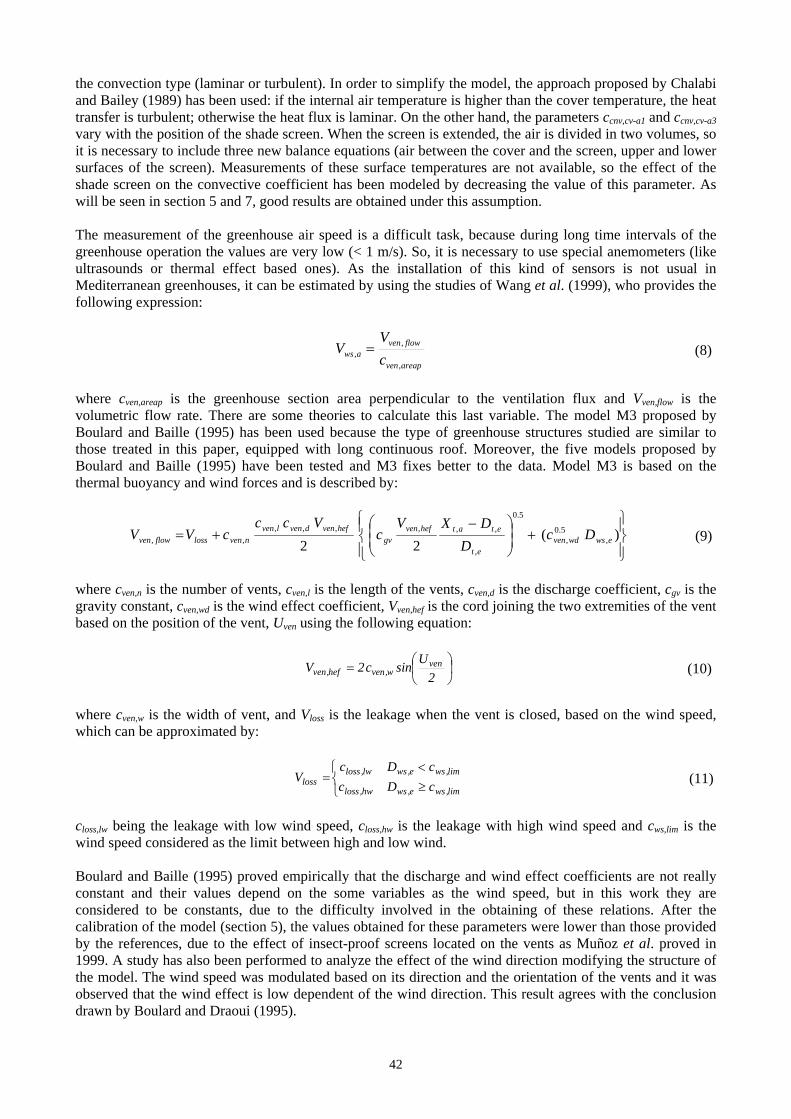
the convection type (laminar or turbulent). In order to simplify the model, the approach proposed by Chalabi and Bailey (1989) has been used: if the internal air temperature is higher than the cover temperature, the heat transfer is turbulent; otherwise the heat flux is laminar. On the other hand, the parameters ccnv,cv-a1 and ccnv,cv-a3 vary with the position of the shade screen. When the screen is extended, the air is divided in two volumes, so it is necessary to include three new balance equations (air between the cover and the screen, upper and lower surfaces of the screen). Measurements of these surface temperatures are not available, so the effect of the shade screen on the convective coefficient has been modeled by decreasing the value of this parameter. As will be seen in section 5 and 7, good results are obtained under this assumption. The measurement of the greenhouse air speed is a difficult task, because during long time intervals of the greenhouse operation the values are very low (< 1 m/s). So, it is necessary to use special anemometers (like ultrasounds or thermal effect based ones). As the installation of this kind of sensors is not usual in Mediterranean greenhouses, it can be estimated by using the studies of Wang et al. (1999), who provides the following expression:

areapven

flowvenaws c

VV

,

,, (8)

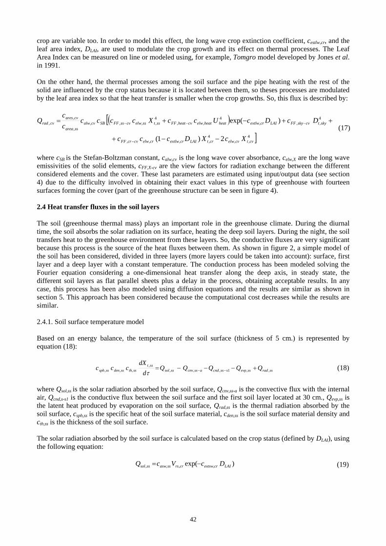
where cven,areap is the greenhouse section area perpendicular to the ventilation flux and Vven,flow is the volumetric flow rate. There are some theories to calculate this last variable. The model M3 proposed by Boulard and Baille (1995) has been used because the type of greenhouse structures studied are similar to those treated in this paper, equipped with long continuous roof. Moreover, the five models proposed by Boulard and Baille (1995) have been tested and M3 fixes better to the data. Model M3 is based on the thermal buoyancy and wind forces and is described by:

)(

22 ,5.0

,

5.0

,

,,,,,,

,, ewswdvenet

etathefvengv

hefvendvenlven

nvenlossflowven DcD

DXVc

VcccVV (9)

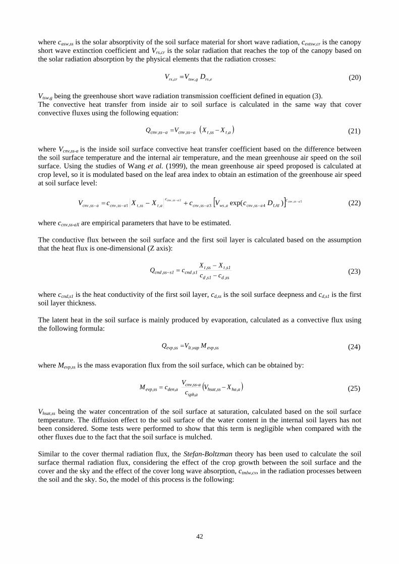
where cven,n is the number of vents, cven,l is the length of the vents, cven,d is the discharge coefficient, cgv is the gravity constant, cven,wd is the wind effect coefficient, Vven,hef is the cord joining the two extremities of the vent based on the position of the vent, Uven using the following equation:

2

Usinc2V ven

w,venhef,ven (10)

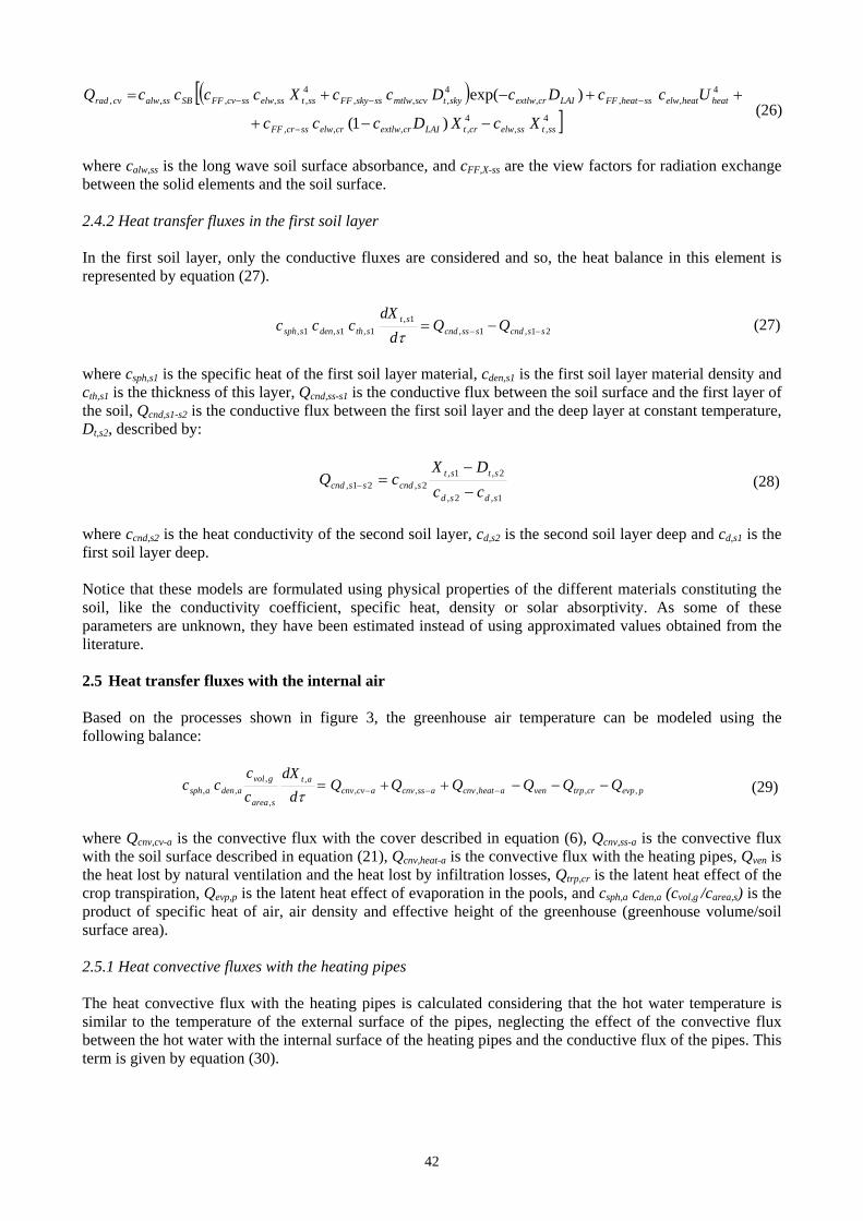
where cven,w is the width of vent, and Vloss is the leakage when the vent is closed, based on the wind speed, which can be approximated by:

lim,wse,wshw,loss

lim,wse,wslw,lossloss cDc

cDcV (11)

closs,lw being the leakage with low wind speed, closs,hw is the leakage with high wind speed and cws,lim is the wind speed considered as the limit between high and low wind. Boulard and Baille (1995) proved empirically that the discharge and wind effect coefficients are not really constant and their values depend on the some variables as the wind speed, but in this work they are considered to be constants, due to the difficulty involved in the obtaining of these relations. After the calibration of the model (section 5), the values obtained for these parameters were lower than those provided by the references, due to the effect of insect-proof screens located on the vents as Muñoz et al. proved in 1999. A study has also been performed to analyze the effect of the wind direction modifying the structure of the model. The wind speed was modulated based on its direction and the orientation of the vents and it was observed that the wind effect is low dependent of the wind direction. This result agrees with the conclusion drawn by Boulard and Draoui (1995).

42

2.3.3 Convective heat transfer from outside air to cover The convective heat transfer from outside air to cover is calculated in a similar way than the inside convective term, using the formula:

et,cv,tssarea,

cvarea,ecv,cnvecv,cnv DX

c

c VQ (12)

where Vcnv,cv-e is the cover outside convective heat transfer coefficient based on the difference between the cover temperature and the external air temperature, Dt,e, and on the outside wind speed. In this case, the wind effect is predominant, so the temperature effect has been neglected. Some authors (e.g. Bot, 1983) proposed a linear relationship with the wind speed and others (e.g. Bailey, 1984) proposed an exponential one. Both approaches have been tested in this work and the data fixed better using a mixed formula including a linear equation for low wind and an exponential equation for high wind speed conditions. This formula is used by other authors as indicated by Boisson (1991):

lim,wse,ws4ecv,cnve,ws3ecv,cnv

lim,wse,wsc

1ecv,cnvecv,cnv

cDcDc

cDDcV

2ecv,cnv

e,ws (13)

where ccnv,cv-eX are empirical parameters which have to be estimated (see section 4). Notice that this formula introduces a switch in the simulation process. As will be commented, the used simulation packages (both block-oriented ones as Simulink and object-oriented one as Modelica) can cope with this kind of behaviour. The same happens for instance with equations (3), (11) and (16). 2.3.4 Latent heat produced by condensation The most important latent convective fluxes on the cover are produced by condensation on the inside surface and so, the condensation on the outside surface can be neglected. Condensation takes place when the water vapour concentration of the internal air, Xha,a, is greater than the water concentration of the cover at saturation, Vhsat,cv, calculated based on the cover temperature. This flux can be written as:

cv,cdvap,ltcv,cd MVQ (14) where Vlt,vap is the latent heat of vaporation of water calculated at internal air temperature (in ºC) using the following equation:

a,tvap,lt X56.05975.4185V (15) Mcd,cv is the mass condensation flux from the cover calculated based on a convective term:

cv,hsathaa,hacv,hsatssarea,

cvarea,

asph,

a-cvcnv,a,den

cv,hsata,h

cv,cd VXXVc

c

c

V c

VX0

M (16)

where csph,a is the specific heat of air and cden,a is the air density. 2.3.5 Thermal radiation absorbed by the cover The cover thermal radiation flux can be calculated using the Stefan-Boltzman theory subtracting the thermal radiation emitted by the cover (two surfaces) and the thermal radiation emitted by the other solid elements of the greenhouse: internal soil surface (ss), pipe heating (heat), crop (cr) and upper hemisphere (sky), that reach the cover surface (the effect of the outside soil surface is neglected). The crop is a solid whose surface and volume are variables in time, so the thermal radiation processes between the rest of the solids and the

42

crop are variable too. In order to model this effect, the long wave crop extinction coefficient, cestlw,cr, and the leaf area index, DLAI, are used to modulate the crop growth and its effect on thermal processes. The Leaf Area Index can be measured on line or modeled using, for example, Tomgro model developed by Jones et al. in 1991. On the other hand, the thermal processes among the soil surface and the pipe heating with the rest of the solid are influenced by the crop status because it is located between them, so theses processes are modulated by the leaf area index so that the heat transfer is smaller when the crop growths. So, this flux is described by:

4

,,4,,,,

4,,,

4,,

4,,,,

,

,,

2)1(

)exp(

cvtcvelwcrtLAIcrextlwcrelwcvcrFF

skytcvskyFFLAIcrextlwheatheatelwcvheatFFsstsselwcvssFFSBcvalwssarea

cvarescvrad

XcXDccc

DcDcUccXccccc

cQ

(17)

where cSB is the Stefan-Boltzman constant, calw,cv is the long wave cover absorbance, celw,X are the long wave emissivities of the solid elements, cFF,X-cv are the view factors for radiation exchange between the different considered elements and the cover. These last parameters are estimated using input/output data (see section 4) due to the difficulty involved in obtaining their exact values in this type of greenhouse with fourteen surfaces forming the cover (part of the greenhouse structure can be seen in figure 4). 2.4 Heat transfer fluxes in the soil layers The soil (greenhouse thermal mass) plays an important role in the greenhouse climate. During the diurnal time, the soil absorbs the solar radiation on its surface, heating the deep soil layers. During the night, the soil transfers heat to the greenhouse environment from these layers. So, the conductive fluxes are very significant because this process is the source of the heat fluxes between them. As shown in figure 2, a simple model of the soil has been considered, divided in three layers (more layers could be taken into account): surface, first layer and a deep layer with a constant temperature. The conduction process has been modeled solving the Fourier equation considering a one-dimensional heat transfer along the deep axis, in steady state, the different soil layers as flat parallel sheets plus a delay in the process, obtaining acceptable results. In any case, this process has been also modeled using diffusion equations and the results are similar as shown in section 5. This approach has been considered because the computational cost decreases while the results are similar. 2.4.1. Soil surface temperature model Based on an energy balance, the temperature of the soil surface (thickness of 5 cm.) is represented by equation (18):

ssradssevpssscndasscnvsssolsst

ssthssdensssph QQQQQd

dXccc ,,1,,,

,,,,

(18)

where Qsol,ss is the solar radiation absorbed by the soil surface, Qcnv,ss-a is the convective flux with the internal air, Qcnd,s-s1 is the conductive flux between the soil surface and the first soil layer located at 30 cm., Qevp,ss is the latent heat produced by evaporation on the soil surface, Qrad,ss is the thermal radiation absorbed by the soil surface, csph,ss is the specific heat of the soil surface material, cden,ss is the soil surface material density and cth,ss is the thickness of the soil surface. The solar radiation absorbed by the soil surface is calculated based on the crop status (defined by DLAI), using the following equation:

)exp( ,,,, LAIcrextswcrrsssaswsssol DcVcQ (19)

42

where casw,ss is the solar absorptivity of the soil surface material for short wave radiation, cextsw,cr is the canopy short wave extinction coefficient and Vrs,cr is the solar radiation that reaches the top of the canopy based on the solar radiation absorption by the physical elements that the radiation crosses:

ersgtswcrrs DVV ,,, (20) Vtsw,g being the greenhouse short wave radiation transmission coefficient defined in equation (3). The convective heat transfer from inside air to soil surface is calculated in the same way that cover convective fluxes using the following equation:

a,tss,tass,cnvass,cnv XX VQ (21) where Vcnv,ss-a is the inside soil surface convective heat transfer coefficient based on the difference between the soil surface temperature and the internal air temperature, and the mean greenhouse air speed on the soil surface. Using the studies of Wang et al. (1999), the mean greenhouse air speed proposed is calculated at crop level, so it is modulated based on the leaf area index to obtain an estimation of the greenhouse air speed at soil surface level:

5,2, )exp( 4,,3,,,1,,asscnvasscnv c

LAIasscnvawsasscnv

c

atsstasscnvasscnv DcVcXXcV

(22)

where ccnv,ss-aX are empirical parameters that have to be estimated. The conductive flux between the soil surface and the first soil layer is calculated based on the assumption that the heat flux is one-dimensional (Z axis):

ss,d1s,d

1s,tss,t1s,cnd1sss,cnd cc

XXcQ

(23)

where ccnd,s1 is the heat conductivity of the first soil layer, cd,ss is the soil surface deepness and cd,s1 is the first soil layer thickness. The latent heat in the soil surface is mainly produced by evaporation, calculated as a convective flux using the following formula:

ss,evpvap,ltss,evp MVQ (24) where Mevp,ss is the mass evaporation flux from the soil surface, which can be obtained by:

a,hass,hsatasph,

a-cnv,ssa,denss,evp XV

c

V cM (25)

Vhsat,ss being the water concentration of the soil surface at saturation, calculated based on the soil surface temperature. The diffusion effect to the soil surface of the water content in the internal soil layers has not been considered. Some tests were performed to show that this term is negligible when compared with the other fluxes due to the fact that the soil surface is mulched. Similar to the cover thermal radiation flux, the Stefan-Boltzman theory has been used to calculate the soil surface thermal radiation flux, considering the effect of the crop growth between the soil surface and the cover and the sky and the effect of the cover long wave absorption, ctmlw,cv, in the radiation processes between the soil and the sky. So, the model of this process is the following:

42

4

,,4,,,,

4,,,

4,,,

4,,,,,

)1(

)exp(

sstsselwcrtLAIcrextlwcrelwsscrFF

heatheatelwssheatFFLAIcrextlwskytscvmtlwssskyFFsstsselwsscvFFSBssalwcvrad

XcXDccc

UccDcDccXccccQ

(26)

where calw,ss is the long wave soil surface absorbance, and cFF,X-ss are the view factors for radiation exchange between the solid elements and the soil surface. 2.4.2 Heat transfer fluxes in the first soil layer In the first soil layer, only the conductive fluxes are considered and so, the heat balance in this element is represented by equation (27).

21,1,1,

1,1,1, sscndssscndst

sthsdenssph QQd

dXccc

(27)

where csph,s1 is the specific heat of the first soil layer material, cden,s1 is the first soil layer material density and cth,s1 is the thickness of this layer, Qcnd,ss-s1 is the conductive flux between the soil surface and the first layer of the soil, Qcnd,s1-s2 is the conductive flux between the first soil layer and the deep layer at constant temperature, Dt,s2, described by:

1,2,

2,1,2,21,

sdsd

ststscndsscnd cc

DXcQ

(28)

where ccnd,s2 is the heat conductivity of the second soil layer, cd,s2 is the second soil layer deep and cd,s1 is the first soil layer deep. Notice that these models are formulated using physical properties of the different materials constituting the soil, like the conductivity coefficient, specific heat, density or solar absorptivity. As some of these parameters are unknown, they have been estimated instead of using approximated values obtained from the literature. 2.5 Heat transfer fluxes with the internal air Based on the processes shown in figure 3, the greenhouse air temperature can be modeled using the following balance:

pevpcrtrpvenaheatcnvasscnvacvcnvat

sarea

gvoladenasph QQQQQQ

d

dX

c

ccc ,,,,,

,

,

,,,

(29)

where Qcnv,cv-a is the convective flux with the cover described in equation (6), Qcnv,ss-a is the convective flux with the soil surface described in equation (21), Qcnv,heat-a is the convective flux with the heating pipes, Qven is the heat lost by natural ventilation and the heat lost by infiltration losses, Qtrp,cr is the latent heat effect of the crop transpiration, Qevp,p is the latent heat effect of evaporation in the pools, and csph,a cden,a (cvol,g /carea,s) is the product of specific heat of air, air density and effective height of the greenhouse (greenhouse volume/soil surface area). 2.5.1 Heat convective fluxes with the heating pipes The heat convective flux with the heating pipes is calculated considering that the hot water temperature is similar to the temperature of the external surface of the pipes, neglecting the effect of the convective flux between the hot water with the internal surface of the heating pipes and the conductive flux of the pipes. This term is given by equation (30).

42

atheattarea,ss

area,heataheatcnvaheatcnv XUVQ ,,,, c

c (30)

where carea,heat is the heat pipe surface, Ut,heat is the water temperature into the heating pipes and Vcnv,heat-a is the heating convective heat transfer coefficient calculated in the same way that the rest of convective coefficients:

)exp( 55,

2,

4,,3,,

,,1,,

aheatcnv

aheatcnv

cLAIaheatcnvawsaheatcnv

c

heatcl

atheattaheatcnvaheatcnv DcVc

c

XUcV

(31)

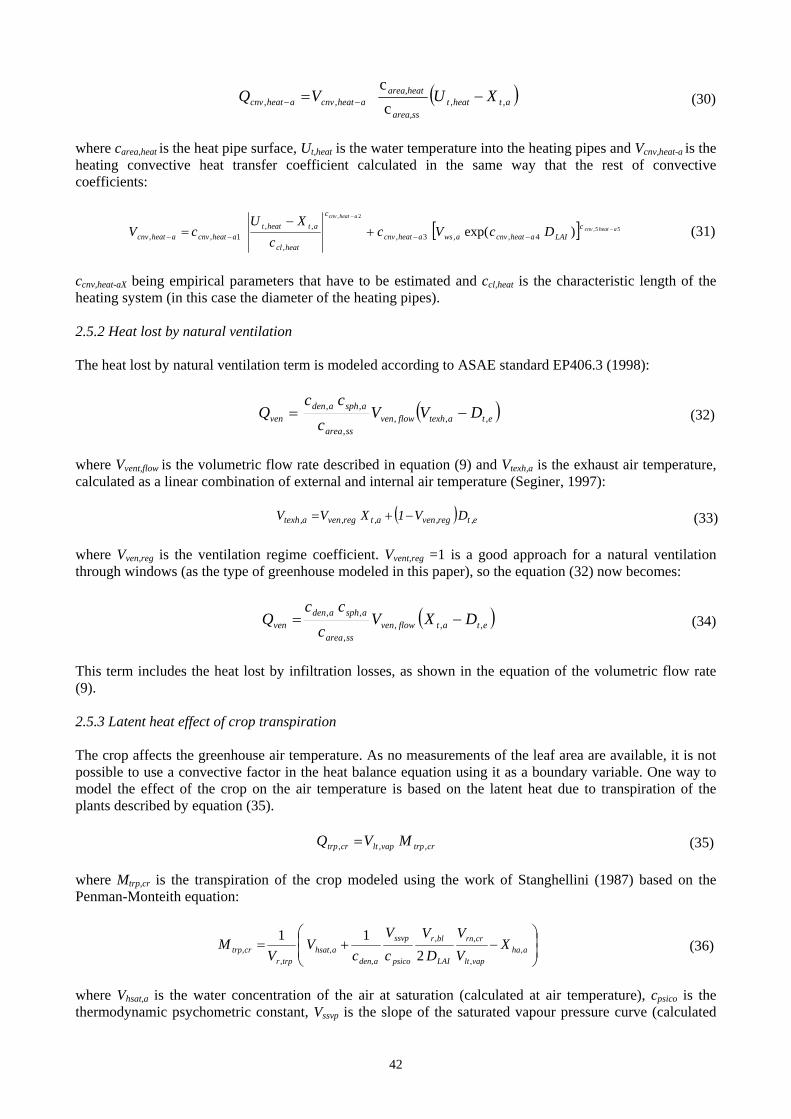
ccnv,heat-aX being empirical parameters that have to be estimated and ccl,heat is the characteristic length of the heating system (in this case the diameter of the heating pipes). 2.5.2 Heat lost by natural ventilation The heat lost by natural ventilation term is modeled according to ASAE standard EP406.3 (1998):

etatexhflowvenssarea

asphadenven DVV

c

ccQ ,,,

,

,, (32)

where Vvent,flow is the volumetric flow rate described in equation (9) and Vtexh,a is the exhaust air temperature, calculated as a linear combination of external and internal air temperature (Seginer, 1997):

e,treg,vena,treg,vena,texh DV1XVV (33) where Vven,reg is the ventilation regime coefficient. Vvent,reg =1 is a good approach for a natural ventilation through windows (as the type of greenhouse modeled in this paper), so the equation (32) now becomes:

etatflowvenssarea

asphadenven DXV

c

ccQ ,,,

,

,, (34)

This term includes the heat lost by infiltration losses, as shown in the equation of the volumetric flow rate (9). 2.5.3 Latent heat effect of crop transpiration The crop affects the greenhouse air temperature. As no measurements of the leaf area are available, it is not possible to use a convective factor in the heat balance equation using it as a boundary variable. One way to model the effect of the crop on the air temperature is based on the latent heat due to transpiration of the plants described by equation (35).

crtrpvapltcrtrp MVQ ,,, (35)

where Mtrp,cr is the transpiration of the crop modeled using the work of Stanghellini (1987) based on the Penman-Monteith equation:

aha

vaplt

crrn

LAI

blr

psico

ssvp

adenahsat

trprcrtrp X

V

V

D

V

c

V

cV

VM ,

,

,,

,,

,, 2

11 (36)

where Vhsat,a is the water concentration of the air at saturation (calculated at air temperature), cpsico is the thermodynamic psychometric constant, Vssvp is the slope of the saturated vapour pressure curve (calculated

42

using the air temperature), Vrn,cr is the net radiation available to the canopy (calculated in the basis of solar radiation), Vr,trp is a transpiration resistance described by the expression (37):

srblr

psico

ssvp

LAItrpr VV

c

V

DV ,,, 1

2

1 (37)

Vr,bl is the boundary layer resistance and Vr,s is the stomatal resistance. Vr,bl depends on the aerodynamic regime that prevails in the greenhouse. Boulard and Wang (2000) neglected the buoyancy effect compared with the wind effect, so this resistance can be expressed with respect to the average inside air speed using expression (38).

8.0a,ws

2.0cr,cl

bl,rV

c220V (38)

where ccl,cr is the characteristic length of the crop leaf. Vr,s depends on the global radiation on the crop, the greenhouse humidity and the crop temperature (Stanghellini and de Jong, 1995). For greenhouse tomato crops, the effect of the global radiation is the most important, so it can be calculated using the following formula (Boulard and Wang, 2000):

))50V05.0exp(

11200V

cr,rss,r (39)

2.5.4. Latent heat effect of the evaporation in the pools The cultivation method of the tomato crop used in the installations is NFT (Nutrient Films Technique). The greenhouse contains non-isolated pools in order to recycle the fertilized water to maintain the continuous water flow. The evaporation of the water of the pools affects the greenhouse climate. In the same way the transpiration of the crop has been included in the balances, a factor has been added to the latent heat term:

p,evpvap,ltp,evp MVQ (40) where Mevp,p is the evaporation flux from the pools. The evaporation from an open water surface is produced by two main factors: the energy to provide the vaporization latent heat (solar radiation) and the capacity to move the water vapour out of the evaporation surface due to wind speed and the air humidity on the surface. The evaporation can be calculated by mixing the aerodynamic method based on the vapour pressure deficit and the energy method based on the energy balance (Chow et al., 1994). This mixed method is adequate for small surfaces with known climate conditions and so, the following equation has been used:

avpdevppsicossvp

psicossrnevp

psicossvp

ssvppevp Vc

cV

cVc

cV

VM ,2,,1,,

(41)

where cevp,1 is a factor to calibrate the effect of the net radiation on the soil surface and cevp,2 is a factor to calibrate the effect of the air vapour pressure deficit, Vvpd,a calculated by:

100

X1VV a,hr

a,vpsata,vpd (42)

where Vvpsat,a is the saturation vapour pressure calculated as an exponential function of the internal air temperature and Xhr,a is the relative humidity calculated in the basis of the absolute humidity, Xha,a (modeled in equation (44)) using the following expression:

42

a,vpsat

a,ta,haa,dena,hr V

XX

00217.0

cX (43)

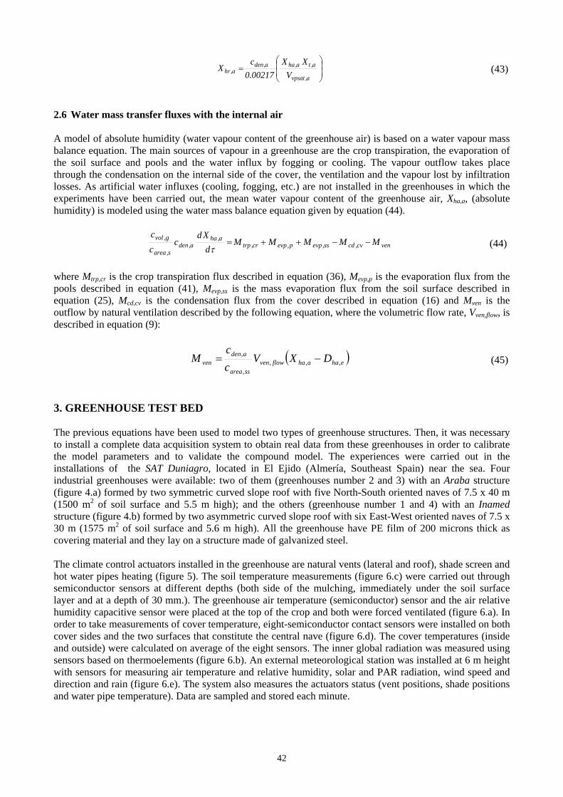
2.6 Water mass transfer fluxes with the internal air A model of absolute humidity (water vapour content of the greenhouse air) is based on a water vapour mass balance equation. The main sources of vapour in a greenhouse are the crop transpiration, the evaporation of the soil surface and pools and the water influx by fogging or cooling. The vapour outflow takes place through the condensation on the internal side of the cover, the ventilation and the vapour lost by infiltration losses. As artificial water influxes (cooling, fogging, etc.) are not installed in the greenhouses in which the experiments have been carried out, the mean water vapour content of the greenhouse air, Xha,a, (absolute humidity) is modeled using the water mass balance equation given by equation (44).

vencv,cdss,evpp,evpcr,trpa,ha

a,dens,area

g,volMMMMM

d

Xdc

c

c

(44)

where Mtrp,cr is the crop transpiration flux described in equation (36), Mevp,p is the evaporation flux from the pools described in equation (41), Mevp,ss is the mass evaporation flux from the soil surface described in equation (25), Mcd,cv is the condensation flux from the cover described in equation (16) and Mven is the outflow by natural ventilation described by the following equation, where the volumetric flow rate, Vven,flow, is described in equation (9):

ehaahaflowvenssarea

adenven DXV

c

cM ,,,

,

, (45)

3. GREENHOUSE TEST BED The previous equations have been used to model two types of greenhouse structures. Then, it was necessary to install a complete data acquisition system to obtain real data from these greenhouses in order to calibrate the model parameters and to validate the compound model. The experiences were carried out in the installations of the SAT Duniagro, located in El Ejido (Almería, Southeast Spain) near the sea. Four industrial greenhouses were available: two of them (greenhouses number 2 and 3) with an Araba structure (figure 4.a) formed by two symmetric curved slope roof with five North-South oriented naves of 7.5 x 40 m (1500 m2 of soil surface and 5.5 m high); and the others (greenhouse number 1 and 4) with an Inamed structure (figure 4.b) formed by two asymmetric curved slope roof with six East-West oriented naves of 7.5 x 30 m (1575 m2 of soil surface and 5.6 m high). All the greenhouse have PE film of 200 microns thick as covering material and they lay on a structure made of galvanized steel. The climate control actuators installed in the greenhouse are natural vents (lateral and roof), shade screen and hot water pipes heating (figure 5). The soil temperature measurements (figure 6.c) were carried out through semiconductor sensors at different depths (both side of the mulching, immediately under the soil surface layer and at a depth of 30 mm.). The greenhouse air temperature (semiconductor) sensor and the air relative humidity capacitive sensor were placed at the top of the crop and both were forced ventilated (figure 6.a). In order to take measurements of cover temperature, eight-semiconductor contact sensors were installed on both cover sides and the two surfaces that constitute the central nave (figure 6.d). The cover temperatures (inside and outside) were calculated on average of the eight sensors. The inner global radiation was measured using sensors based on thermoelements (figure 6.b). An external meteorological station was installed at 6 m height with sensors for measuring air temperature and relative humidity, solar and PAR radiation, wind speed and direction and rain (figure 6.e). The system also measures the actuators status (vent positions, shade positions and water pipe temperature). Data are sampled and stored each minute.

42

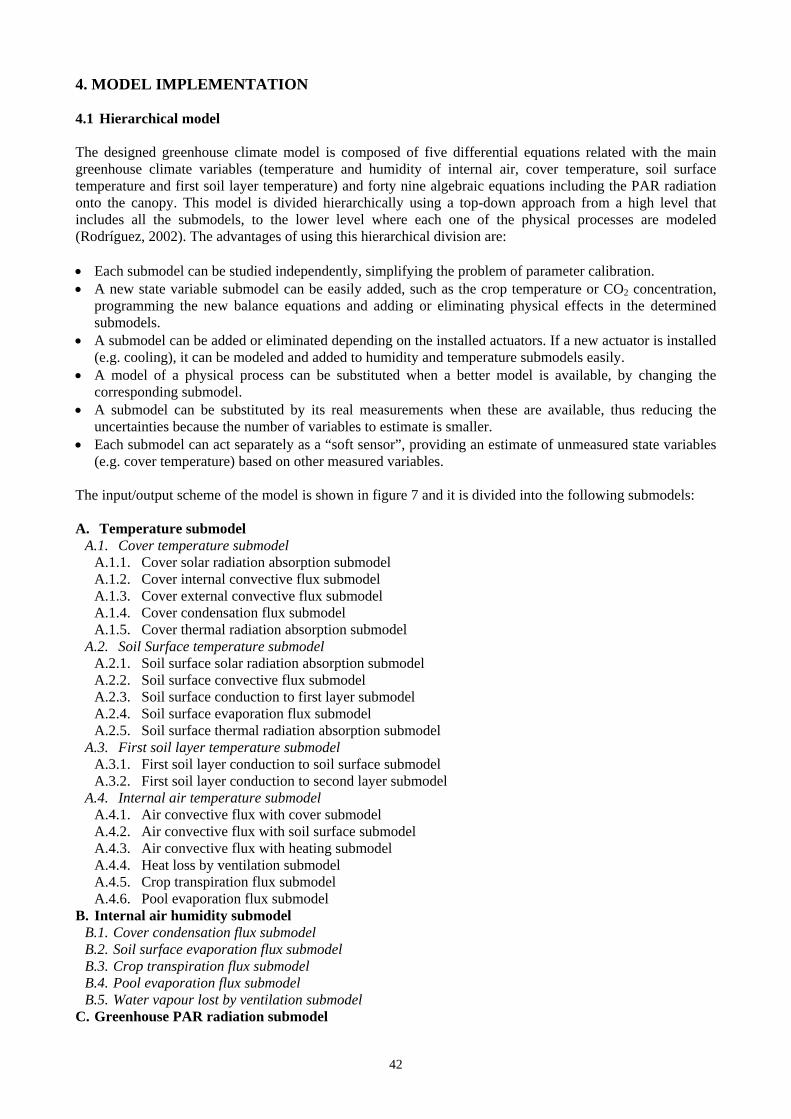
4. MODEL IMPLEMENTATION 4.1 Hierarchical model The designed greenhouse climate model is composed of five differential equations related with the main greenhouse climate variables (temperature and humidity of internal air, cover temperature, soil surface temperature and first soil layer temperature) and forty nine algebraic equations including the PAR radiation onto the canopy. This model is divided hierarchically using a top-down approach from a high level that includes all the submodels, to the lower level where each one of the physical processes are modeled (Rodríguez, 2002). The advantages of using this hierarchical division are: Each submodel can be studied independently, simplifying the problem of parameter calibration. A new state variable submodel can be easily added, such as the crop temperature or CO2 concentration,

programming the new balance equations and adding or eliminating physical effects in the determined submodels.

A submodel can be added or eliminated depending on the installed actuators. If a new actuator is installed (e.g. cooling), it can be modeled and added to humidity and temperature submodels easily.

A model of a physical process can be substituted when a better model is available, by changing the corresponding submodel.

A submodel can be substituted by its real measurements when these are available, thus reducing the uncertainties because the number of variables to estimate is smaller.

Each submodel can act separately as a “soft sensor”, providing an estimate of unmeasured state variables (e.g. cover temperature) based on other measured variables.

The input/output scheme of the model is shown in figure 7 and it is divided into the following submodels: A. Temperature submodel

A.1. Cover temperature submodel A.1.1. Cover solar radiation absorption submodel A.1.2. Cover internal convective flux submodel A.1.3. Cover external convective flux submodel A.1.4. Cover condensation flux submodel A.1.5. Cover thermal radiation absorption submodel

A.2. Soil Surface temperature submodel A.2.1. Soil surface solar radiation absorption submodel A.2.2. Soil surface convective flux submodel A.2.3. Soil surface conduction to first layer submodel A.2.4. Soil surface evaporation flux submodel A.2.5. Soil surface thermal radiation absorption submodel

A.3. First soil layer temperature submodel A.3.1. First soil layer conduction to soil surface submodel A.3.2. First soil layer conduction to second layer submodel

A.4. Internal air temperature submodel A.4.1. Air convective flux with cover submodel A.4.2. Air convective flux with soil surface submodel A.4.3. Air convective flux with heating submodel A.4.4. Heat loss by ventilation submodel A.4.5. Crop transpiration flux submodel A.4.6. Pool evaporation flux submodel

B. Internal air humidity submodel B.1. Cover condensation flux submodel B.2. Soil surface evaporation flux submodel B.3. Crop transpiration flux submodel B.4. Pool evaporation flux submodel B.5. Water vapour lost by ventilation submodel

C. Greenhouse PAR radiation submodel

42

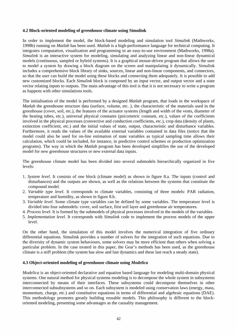
4.2 Block-oriented modeling of greenhouse climate using Simulink In order to implement the model, the block-based modeling and simulation tool Simulink (Mathworks, 1998b) running on Matlab has been used. Matlab is a high-performance language for technical computing. It integrates computation, visualization and programming in an easy-to-use environment (Mathworks, 1998a). Simulink is an interactive system for modeling, simulating and analyzing linear and non-linear dynamical models (continuous, sampled or hybrid systems). It is a graphical mouse-driven program that allows the user to model a system by drawing a block diagram on the screen and manipulating it dynamically. Simulink includes a comprehensive block library of sinks, sources, linear and non-linear components, and connectors, so that the user can build the model using these blocks and connecting them adequately. It is possible to add new customized blocks. Each Simulink block is composed by an input vector, and output vector and a state vector relating inputs to outputs. The main advantage of this tool is that it is not necessary to write a program as happens with other simulations tools. The initialisation of the model is performed by a designed Matlab program, that loads in the workspace of Matlab the greenhouse structure data (surface, volume, etc. ), the characteristic of the materials used in the greenhouse (cover, soil, etc.), the features of the actuator systems (length and width of the vents, diameter of the heating tubes, etc.), universal physical constants (psicometric constant, etc.), values of the coefficients involved in the physical processes (convective and conduction coefficients, etc.), crop data (density of plants, extinction coefficient, etc.) and the initial values of state, output, characteristic and disturbance variables. Furthermore, it reads the values of the available external variables contained in data files (notice that the model could also be used for on-line estimation of state variables as typical sampling time allows their calculation, which could be included, for instance, in predictive control schemes or production optimization programs). The way in which the Matlab program has been developed simplifies the use of the developed model for new greenhouse structures or new external data inputs. The greenhouse climate model has been divided into several submodels hierarchically organized in five levels: 1. System level. It consists of one block (climate model) as shown in figure 8.a. The inputs (control and

disturbances) and the outputs are shown, as well as the relations between the systems that constitute the compound model.

2. Variable type level. It corresponds to climate variables, consisting of three models: PAR radiation, temperature and humidity, as shown in figure 8.b.

3. Variable level. Some climate type variables can be defined by some variables. The temperature level is divided into four submodels: cover, soil surface, first soil layer and greenhouse air temperatures.

4. Process level. It is formed by the submodels of physical processes involved in the models of the variables. 5. Implementation level. It corresponds with Simulink code to implement the process models of the upper

level. On the other hand, the simulation of this model involves the numerical integration of five ordinary differential equations. Simulink provides a number of solvers for the integration of such equations. Due to the diversity of dynamic system behaviours, some solvers may be more efficient than others when solving a particular problem. In the case treated in this paper, the Gear’s methods has been used, as the greenhouse climate is a stiff problem (the system has slow and fast dynamics and these last reach a steady state). 4.3 Object-oriented modeling of greenhouse climate using Modelica Modelica is an object-oriented declarative and equation based language for modeling multi-domain physical systems. One natural method for physical systems modeling is to decompose the whole system in subsystems interconnected by means of their interfaces. These subsystems could decompose themselves in other interconnected subsubsystems and so on. Each subsystem is modeled using conservation laws (energy, mass, momentum, charge, etc.) and constitutive equations in terms of differential and algebraic equations (DAE). This methodology promotes greatly building reusable models. This philosophy is different to the block-oriented modeling, presenting some advantages as the causality management.

42

In order to develop the model of the compound greenhouse climate model using Modelica, the OMT (Object Modeling Technique) methodology, proposed by Rumbaugh et al. (1991) has been used. This technique proposes a formal graph showing the relations (association, aggregation and generalization) between the different objects that constitute the systems and their properties and attributes. Three general classes have been defined (Rodríguez et al., 2002): Crop_model class. It represents the leaf area index (modeled o measured) of a tomato crop. Greenhouse class. This class describes the greenhouse where the simulation test is designed. Its

attributes are the parameters of the different elements constituting the greenhouse. The main advantage of this design is the possibility of changing or adding a physical element (i.e. actuators) easily. These classes are described by their own name: Structure. Type and dimensions of the greenhouse structure. Ventilation. Type and dimensions of the ventilation. Heating. Type and parameters of the heating system. Soil_surface. Type of material of the soil surface. First_layer_soil. Type of material of the first layer soil. Second_layer_soil. Type of material of the second layer soil. Cover. Type of cover material.

Greenhouse_model class. It represents the different models that describe the greenhouse climate variables. It is related with the Greenhouse class to obtain the parameters of the greenhouse where the simulation experiencies are performed. Furthermore, this class is related with the crop_model class to model the effects of the plants on the climate. It is constituted by an aggregation relation of the following classes: Temperature_model. Class of the different models of internal air temperature. Humidity_model. Class of the different models of internal air humidity. Cover_model. Class of the different models of cover temperature. Soil_model. It is formed by two subclasses:

o Soil_surface_model. Class of the different models of soil surface temperature. o Soil_layer_model. Class of the different models of the soil layer temperature.

The compound model is defined by five ordinary differential equations and fifty eight algebraic equations. This equation system is solved using the DASSL algorithm (Brenan et al., 1989) because the simulation computational time was the smallest and it is very efficient to solve stiff systems. 5. MODEL CALIBRATION 5.1. The problem of model calibration and the proposed methodology Due to the large set of unknown parameters (more than thirty), it is very difficult to obtain their values using a unique search technique with the compound model. The solution consists in performing single experimental tests for each one of the involved processes to estimate their parameters, in a similar way to the experiences carried out by Bot (1983). These experiments are not easy to be performed, and some of them are very expensive and present a long duration. On the other hand, gthe input/output meteorological and actuator status data are often at hand in a typical greenhouse instalation, so it would be desirable to use only these data to calibrate the greenhouse climate model, without loosing the physical meaning of the processes involved in the balace equations. This problem can be simplified considering the following facts: Data of the different climate variables to model, the disturbances and the actuators status are measured, so

the problem has been divided into some submodels calibration processes (air humidity and cover, air, soil surface and first soil layer temperature).

Some of the involved physical processes in the balance equations are not coupled or they have no influence in determined time lapses of a day (e.g. the solar absorbance during the night or the crop presence), so all the parameters of a single submodel do not have to be estimated simultaneously.

42

Some of the involved physical processes have been modeled in different forms based on determined situations (as the convection process between the internal side of the cover and the greenhouse air in which the parameters of the convection coefficient are different depending on laminar or turbulent regimes). So, the calibration process can be divided for each one of these situations.

In order to estimate the parameters related to the actuation systems some guided test (mainly step response and impulse response ones) can be performed at the real greenhouse.

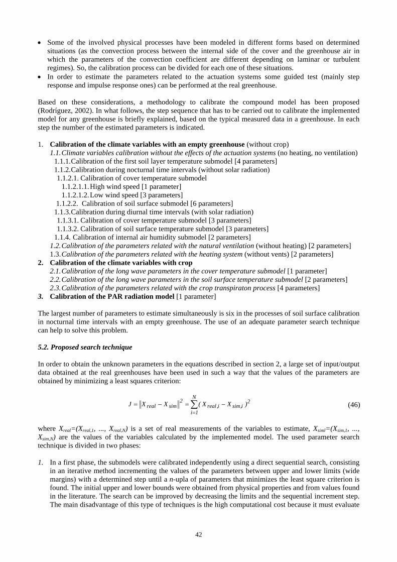
Based on these considerations, a methodology to calibrate the compound model has been proposed (Rodríguez, 2002). In what follows, the step sequence that has to be carried out to calibrate the implemented model for any greenhouse is briefly explained, based on the typical measured data in a greenhouse. In each step the number of the estimated parameters is indicated. 1. Calibration of the climate variables with an empty greenhouse (without crop)

1.1. Climate variables calibration without the effects of the actuation systems (no heating, no ventilation) 1.1.1. Calibration of the first soil layer temperature submodel [4 parameters] 1.1.2. Calibration during nocturnal time intervals (without solar radiation) 1.1.2.1. Calibration of cover temperature submodel

1.1.2.1.1. High wind speed [1 parameter] 1.1.2.1.2. Low wind speed [3 parameters]

1.1.2.2. Calibration of soil surface submodel [6 parameters] 1.1.3. Calibration during diurnal time intervals (with solar radiation) 1.1.3.1. Calibration of cover temperature submodel [3 parameters] 1.1.3.2. Calibration of soil surface temperature submodel [3 parameters]

1.1.4. Calibration of internal air humidity submodel [2 parameters] 1.2. Calibration of the parameters related with the natural ventilation (without heating) [2 parameters] 1.3. Calibration of the parameters related with the heating system (without vents) [2 parameters]

2. Calibration of the climate variables with crop 2.1. Calibration of the long wave parameters in the cover temperature submodel [1 parameter] 2.2. Calibration of the long wave parameters in the soil surface temperature submodel [2 parameters] 2.3. Calibration of the parameters related with the crop transpiraton process [4 parameters]

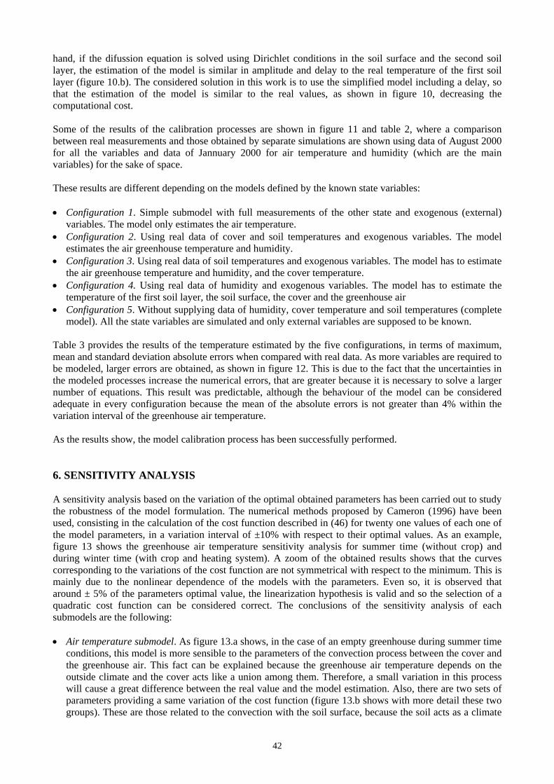
3. Calibration of the PAR radiation model [1 parameter] The largest number of parameters to estimate simultaneously is six in the processes of soil surface calibration in nocturnal time intervals with an empty greenhouse. The use of an adequate parameter search technique can help to solve this problem. 5.2. Proposed search technique In order to obtain the unknown parameters in the equations described in section 2, a large set of input/output data obtained at the real greenhouses have been used in such a way that the values of the parameters are obtained by minimizing a least squares criterion:

N

1i

2i,simi,real

2simreal )XX(XXJ (46)

where Xreal=(Xreal,1, ..., Xreal,N) is a set of real measurements of the variables to estimate, Xsiml=(Xsim,1, ..., Xsim,N) are the values of the variables calculated by the implemented model. The used parameter search technique is divided in two phases: 1. In a first phase, the submodels were calibrated independently using a direct sequential search, consisting

in an iterative method incrementing the values of the parameters between upper and lower limits (wide margins) with a determined step until a n-upla of parameters that minimizes the least square criterion is found. The initial upper and lower bounds were obtained from physical properties and from values found in the literature. The search can be improved by decreasing the limits and the sequential increment step. The main disadvantage of this type of techniques is the high computational cost because it must evaluate

42

all the values of the search space. So, it is used to obtain only approximated values of the model parameters, reducing the search space.

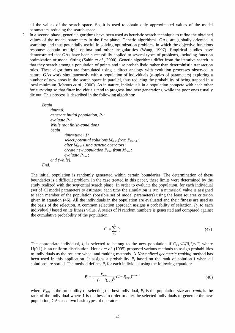
2. In a second phase, genetic algorithms have been used as heuristic search technique to refine the obtained values of the model parameters in the first phase. Genetic algorithms, GAs, are globally oriented in searching and thus potentially useful in solving optimization problems in which the objective functions response contain multiple optima and other irregularities (Wang, 1997). Empirical studies have demonstrated that GAs have been successfully applied to several types of problems, including function optimization or model fitting (Sahin et al., 2000). Genetic algorithms differ from the iterative search in that they search among a population of points and use probabilistic rather than deterministic transaction rules. These algorithms are formulated using a direct analogy with evolution processes observed in nature. GAs work simultaneously with a population of individuals (n-uplas of parameters) exploring a number of new areas in the search space in parallel, thus reducing the probability of being trapped in a local minimum (Matous et al., 2000). As in nature, individuals in a population compete with each other for surviving so that fitter individuals tend to progress into new generations, while the poor ones usually die out. This process is described in the following algorithm:

Begin time=0; generate initial population, P0; evaluate P0; While (not finish-condition) begin time=time+1; select potential solutions Mtime from Ptime-1; alter Mtime using genetic operators; create new population Ptime from Mtime; evaluate Ptime; end (while); End.

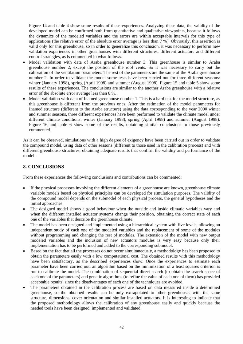
The initial population is randomly generated within certain boundaries. The determination of these boundaries is a difficult problem. In the case treated in this paper, these limits were determined by the study realized with the sequential search phase. In order to evaluate the population, for each individual (set of all model parameters to estimate) each time the simulation is run, a numerical value is assigned to each member of the population (possible set of model parameters) using the least squares criterion given in equation (46). All the individuals in the population are evaluated and their fitness are used as the basis of the selection. A common selection approach assigns a probability of selection, Pj, to each individual j based on its fitness value. A series of N random numbers is generated and compared against the cumulative probability of the population:

i

1jji PC (47)

The appropriate individual, i, is selected to belong to the new population if Ci-1<U(0,1)<Ci where U(0,1) is an uniform distribution. Houck et al. (1995) proposed various methods to assign probabilities to individuals as the roulette wheel and ranking methods. A Normalized geometric ranking method has been used in this application. It assigns a probability Pi based on the rank of solution i when all solutions are sorted. The method defines Pi for each individual using the following equation:

1rankbestP

best

besti

i

s)P1(

)P1(1

PP

(48)

where Pbest is the probability of selecting the best individual, Ps is the population size and ranki is the rank of the individual where 1 is the best. In order to alter the selected individuals to generate the new population, GAs used two basic types of operators:

42

Crossover. This operator takes two individuals and produces two new individuals exchanging genetic

information in pairs or larger group between the parents. There are some crossover operators and in this application the Real-Value Simple crossover has been used. Let X and Y two m-dimensional row vectors of floats denoting individuals from the population. This operator generates a random number n from an uniform distribution U(0,1) and creates two new individuals X’ and Y’ based on the following equations:

nYX)n1('Y

Y)n1(Xn'X

(49)

Mutation. This operator alters one individual to produce a single new solution. An Uniform mutation

algorithm has been used, that selects randomly one variable j, and sets it equal to an uniform random number U(ai,bi) where ai and bi are the lower and upper bounds for the variable i:

jiifx

jiif)b,a(U'x

i

iii (50)

Table 1 (mean absolute error, maximum absolute error and standard deviation) and figure 9 show that the estimation of the coefficients using GAs methods is better than the iterative search for the complete model. Furthermore, this technique is more efficient in time. Although it is necessary to indicate that, the search space of the initial population was reduced because it was deduced of the study carry out with the sequential search of the simple submodels. 5.3. Results of the calibration process In order to calibrate the parameters of the greenhouse climate models two experiencies have been performed in the Araba and Inamed greenhouses: one in summer season (without crop and with guided experiences using the natural ventilations) during July and August 2000, and other in winter season (with tomato crop and guided experiences using the heating system) during January 2000. Data of fifteen days with one minute sample time (21600 real measurements) have been used in the calibration phase in each experience. In order to calibrate the PAR radiation, modeled by an algebraic equation, data of a month without whitening have been used (January 2000) to verify the data provided by the manufacturers of the cover material and the shade screen. The values have been slightly corrected because they loose the original properties along time. This variation of the parameters is not accounted for by the model because the chemical equations that describe the degradation of the physical characteristics are not known. In any case the degradation process takes place slowly, so it is logical to suppose that these parameters are constant during a simulation experiment (during one season at the most). It is obviously necessary to calibrate these values along time. The used data to calibrate the effect on the transmission coefficient of the cover when it is whitened, correspond to May and June 2000. The submodels have been independently calibrated because all the needed input/output data have been measured. The calibration process is similar for any greenhouse, so only the obtained results for Araba greenhouse number 2 are shown in this section for the sake of space. It is interesting to show the behavior of the used simplified model of the soil layer temperature. As indicated in section 2.4, the conduction processes between the different soil layers have been modeled considering steady state regime to solve the Fourier equation. The temperature of the first soil layer has been modeled using this approach because there are only conduction processes as energy fluxes. The dynamic response of a soil layer temperature is characterized by a time constant based on the density and specific heat of the material forming the layer and its thickness. Although this approach is commonly used in the literature about greenhouse climate, the model based on the diffusion equation has been implemented and calibrated too, to compare the real first soil layer temperature with the temperature estimated by the simplified model (low computational cost) and that estimated by the difussion model (high computational cost). Figure 10.a shows that the amplitude of the real temperature is similar to the estimation of the simplified model without delay, although both curves are shifted in the time axis. The delay between the real and the simulated temperature is due to the consideration of the steady state regime of the heat transfer between the soil layers. On the other

42

hand, if the difussion equation is solved using Dirichlet conditions in the soil surface and the second soil layer, the estimation of the model is similar in amplitude and delay to the real temperature of the first soil layer (figure 10.b). The considered solution in this work is to use the simplified model including a delay, so that the estimation of the model is similar to the real values, as shown in figure 10, decreasing the computational cost. Some of the results of the calibration processes are shown in figure 11 and table 2, where a comparison between real measurements and those obtained by separate simulations are shown using data of August 2000 for all the variables and data of Jannuary 2000 for air temperature and humidity (which are the main variables) for the sake of space. These results are different depending on the models defined by the known state variables: Configuration 1. Simple submodel with full measurements of the other state and exogenous (external)

variables. The model only estimates the air temperature. Configuration 2. Using real data of cover and soil temperatures and exogenous variables. The model

estimates the air greenhouse temperature and humidity. Configuration 3. Using real data of soil temperatures and exogenous variables. The model has to estimate

the air greenhouse temperature and humidity, and the cover temperature. Configuration 4. Using real data of humidity and exogenous variables. The model has to estimate the

temperature of the first soil layer, the soil surface, the cover and the greenhouse air Configuration 5. Without supplying data of humidity, cover temperature and soil temperatures (complete

model). All the state variables are simulated and only external variables are supposed to be known. Table 3 provides the results of the temperature estimated by the five configurations, in terms of maximum, mean and standard deviation absolute errors when compared with real data. As more variables are required to be modeled, larger errors are obtained, as shown in figure 12. This is due to the fact that the uncertainties in the modeled processes increase the numerical errors, that are greater because it is necessary to solve a larger number of equations. This result was predictable, although the behaviour of the model can be considered adequate in every configuration because the mean of the absolute errors is not greater than 4% within the variation interval of the greenhouse air temperature. As the results show, the model calibration process has been successfully performed. 6. SENSITIVITY ANALYSIS A sensitivity analysis based on the variation of the optimal obtained parameters has been carried out to study the robustness of the model formulation. The numerical methods proposed by Cameron (1996) have been used, consisting in the calculation of the cost function described in (46) for twenty one values of each one of the model parameters, in a variation interval of ±10% with respect to their optimal values. As an example, figure 13 shows the greenhouse air temperature sensitivity analysis for summer time (without crop) and during winter time (with crop and heating system). A zoom of the obtained results shows that the curves corresponding to the variations of the cost function are not symmetrical with respect to the minimum. This is mainly due to the nonlinear dependence of the models with the parameters. Even so, it is observed that around ± 5% of the parameters optimal value, the linearization hypothesis is valid and so the selection of a quadratic cost function can be considered correct. The conclusions of the sensitivity analysis of each submodels are the following: Air temperature submodel. As figure 13.a shows, in the case of an empty greenhouse during summer time

conditions, this model is more sensible to the parameters of the convection process between the cover and the greenhouse air. This fact can be explained because the greenhouse air temperature depends on the outside climate and the cover acts like a union among them. Therefore, a small variation in this process will cause a great difference between the real value and the model estimation. Also, there are two sets of parameters providing a same variation of the cost function (figure 13.b shows with more detail these two groups). These are those related to the convection with the soil surface, because the soil acts as a climate

42

regulator, providing energy during the nocturnal periods. Figure 13.b also shows that the air temperature has low sensitivity to the parameters related to the ventilation process. This is not what was expected, as the ventilation is the main cooling source. Some sensitivity analyses have been performed for diurnal periods of 10 hours where the ventilation was acting during a long time interval, observing that all the obtained results are similar. A possible cause of the obtained result is the low ventilation rate of the ventilation system installed in the analyzed greenhouse. This result should not be extrapolated to other greenhouse structures. In the case of a greenhouse with crop under winter conditions, the temperature of the air is more sensible to the convection process with the heating pipes parameters as figure 13.c shows. Figure 13.d shows a zoom of the influence of the rest of parameters. The results are similar to the previous analysis, where the model is sensible to cover convection parameters, moderately robust to changes in the the parameters of soil convection and quite robust to the variation of the ventilation parameters.

Cover temperature submodel. The cover temperature submodel is quite sensible to the parameters related to long wave radiation between the cover and the rest of the solids (soil, crop and heating system) due to the fact that the temperature difference between the different elements is the source of the processes of heat transmission. The temperature of the heating system is very high compared with that of the other elements, reason of why its effect is larger. The heat transmission by thermal radiation depends on the temperature difference power to 4, reason of why its contribution is very important.

First soil temperature submodel. This model is more sensible to the conduction coefficient with the soil surface as was to be expected. It is observed that the degree of sensitivity with respect to other parameters is of similar order, since the value of the cost function varies between 45 and 48 reason of why a special sensitivity to anyone of the parameters cannot be deduced.

Soil surface temperature submodel. Some of the previous conclusions are extrapolated to the soil surface temperature submodel, which is more sensible to the variation of those parameters related to the processes of thermal radiation. In a second level, the model is more sensible to the conduction processes than to the convection processes with the inner air, due to the fact that the soil is a thermal buffer where the conduction processes are dominant.

Humidity submodel. The sensitivity analysis of the humidity submodel has been divided into two stages. The first one corresponds to a period without crop under summer conditions, where the humidity model is more sensible to the parameters related to the evaporation process in the irrigation pools, mainly with the parameter related to the solar radiation. This is logical as under these conditions, this process is the main source of water contribution to the greenhouse air. On the other hand, it is less sensible to the parameters related to the natural ventilation, as happened with the temperature submodel previously commented. In the second stage a tomato crop with a middle-development state (LAI=3) was considered, where the humidity model is more sensible to the parameters related to the processes of thermal radiation. This is due to the fact that, in this case, the main source of water contribution is the crop transpiration that directly depends on the net radiation that reaches the canopy (related to the short wave and the thermal radiation). The sensitivity to the rest of parameters is similar to that of the first period.

7. MODEL VALIDATION In order to validate the developed model, data of the last seasons have been used, but in these experiences some state variables (cover and soil layers temperatures) were not measured. So, only the configuration 5 of the compound climate model has been used to validate the greenhouse air temperature and humidity. Due to the fact that all the state variables are related, if two of them are validated, it can be expected that the behaviour of the rest of them is adequate. In any case, the estimation of these variables provided by the model has been studied to confirm that their evolution is that expected. The experiences performed to validate the model are the following: Model validation with data of Araba greenhouse number 2. After the calibration the model for this

greenhouse (described in the previous sections) with data of 2000 winter and summer seasons, the following tests have been performed: Evaluation of the model in the same seasons of another year: January and August 1998. Evaluation of the model in a different season of those used in the calibration process: 1998 spring

season.

42

Figure 14 and table 4 show some results of these experiences. Analyzing these data, the validity of the developed model can be confirmed both from quantitative and qualitative viewpoints, because it follows the dynamics of the modeled variables and the errors are within acceptable intervals for this type of applications (the relative error of the absolute error average is less than 7 %). Obviously, this assertion is valid only for this greenhouse, so in order to generalize this conclusion, it was necessary to perform new validation experiences in other greenhouses with different structures, different actuators and different control strategies, as is commented in what follows.

Model validation with data of Araba greenhouse number 3. This greenhouse is similar to Araba greenhouse number 2, except the position of the roof vents. So it was necessary to carry out the calibration of the ventilation parameters. The rest of the parameters are the same of the Araba greenhouse number 2. In order to validate the model some tests have been carried out for three different seasons: winter (January 1998), spring (April 1998) and summer (August 1998). Figure 15 and table 5 show some results of these experiences. The conclusions are similar to the another Araba greenhouse with a relative error of the absolute error average less than 8 %.

Model validation with data of Inamed greenhouse number 1. This is a hard test for the model structure, as this greenhouse is different from the previous ones. After the estimation of the model parameters for Inamed structure (different to the Araba structure) using the data corresponding to the year 2000 winter and summer seasons, three different experiences have been performed to validate the climate model under different climate conditions: winter (January 1998), spring (April 1998) and summer (August 1998). Figure 16 and table 6 show some of the results, obtaining similar conclusions to those previously commented.

As it can be observed, simulations with a high degree of exigency have been carried out in order to validate the compound model, using data of other seasons (different to those used in the calibration process) and with different greenhouse structures, obtaining adequate results that confirm the validity and performance of the model. 8. CONCLUSIONS From these experiences the following conclusions and contributions can be commented: If the physical processes involving the different elements of a greenhouse are known, greenhouse climate

variable models based on physical principles can be developed for simulation purposes. The validity of the compound model depends on the submodel of each physical process, the general hypotheses and the initial approaches.

The designed model shows a good behaviour when the outside and inside climatic variables vary and when the different installed actuator systems change their position, obtaining the correct state of each one of the variables that describe the greenhouse climate.

The model has been designed and implemented using a hierarchical system with five levels, allowing an independent study of each one of the modeled variables and the replacement of some of the modules without programming and changing the rest of modules. The extension of the model with new output modeled variables and the inclusion of new actuators modules is very easy because only their implementation has to be performed and added to the corresponding submodel.

Based on the fact that all the processes do not occur simultaneously, a methodology has been proposed to obtain the parameters easily with a low computational cost. The obtained results with this methodology have been satisfactory, as the described experiences show. Once the experiences to estimate each parameter have been carried out, an algorithm based on the minimization of a least squares criterion is run to calibrate the model. The combination of sequential direct search (to obtain the search space of each one of the parameters) and genetic algorithms (to refine the value of each one of them) has provided acceptable results, since the disadvantages of each one of the techniques are avoided.

The parameters obtained in the calibration process are based on data measured inside a determined greenhouse, so the obtained results can be only extrapolated to other greenhouses with the same structure, dimensions, cover orientation and similar installed actuators. It is interesting to indicate that the proposed methodology allows the calibration of any greenhouse easily and quickly because the needed tools have been designed, implemented and validated.

42

An important advantage of this methodology is that it is not necessary to perform specific and expensive experiences to obtain the parameters of each involved physical process, as the experiences performed by Bot (1983), in which it was necessary to use a high number of sensors and a very precise methodology for each type of process. The proposed methodology only requires the typical climate data measured in a typical greenhouse installation plus cheap sensors of cover and soil layers temperature.

The acceptable results obtained in three independent greenhouses prove the validity of the model, although new experiences could be performed in other structures and other geographic locations with different climate to that of the Spanish Southeast.

The implemented model is a powerful tool that can be used for the design of climate controllers and actuators (for example, width and maximum opening angle of the ventilation, short wave radiation transmission of the shade screen, diameter of the heating pipes, etc.) or to study the effect of different cover materials and soil substrate on the climate.

Two different paradigms have been compared to implement the model (block-oriented and object-oriented modeling), analysing the advantages and disadvantages of each approach for the greenhouse climate modeling.

Until now a compound climate model for the characteristics of the Southeast of Spain had not been developed, although the structures and the climate are similar to the other Mediterranean zones like France, Italy or Greece. The obtained results are comparable and, in some cases, better than those of other simulation models published in the specialized literature.

Obviously, the developed model can be extended by adding submodels of other important climate variables as the CO2 concentration and/or the inclusion of other actuators as forced ventilation or fogging systems, this extension being a quite easy task due to the used modular design. ACKNOWLEDGEMENTS Authors would like to thank CICYT and FEDER for funding this work under grants DPI2002-04375-C03-03, DPI2001-2380-C02-02 and QUI99-0663-C02-02. The authors also thank Luis Yebra from PSA for his help and suggestions in implementing the model in Modelica.

42

Figure 1. Heat transfer fluxes in a cover

Figure 2. Heat transfer fluxes in the soil layers

Figure 3. Heat transfer fluxes with the internal air

Xt,a

Dt,e

Drs,e

Vrs,cr

Xt,cve

Xt,cviQcnv,cv-a

Qcnv,cv-e

Qrad,cvi

Qrad,cve

Qcd,cve

Qcd,cvi

Qsol,cv

cth,cv

Qcnd,cv

Xt,a

Dt,e

Drs,e

Vrs,cr

Xt,cve

Xt,cviQcnv,cv-a

Qcnv,cv-e

Qrad,cvi

Qrad,cve

Qcd,cve

Qcd,cvi

Qsol,cv

cth,cv

Qcnd,cv

Xt,a

X t,cv

Xt,ss

Dt,e

U t, heat

Q cnv ,cv - a

Q loss

Uven

Qevp,p

Pool

Qcnv,ss-a

Q cnv ,h - a

Qven

Qtrp,cr

cth,sscd,s1

cd,s2Dt,s2

Xt,a

Xt,s1

Xt,ss

Drs,e

Qcnv,ss-a

Qrad,ss

Qevp,ss

Qcnd,ss-s1

Vrs,ss

Qcnd,s1-s2

cth,sscd,s1

cd,s2Dt,s2

Xt,a

Xt,s1

Xt,ss

Drs,e

Qcnv,ss-a

Qrad,ss

Qevp,ss

Qcnd,ss-s1

Vrs,ss

Qcnd,s1-s2

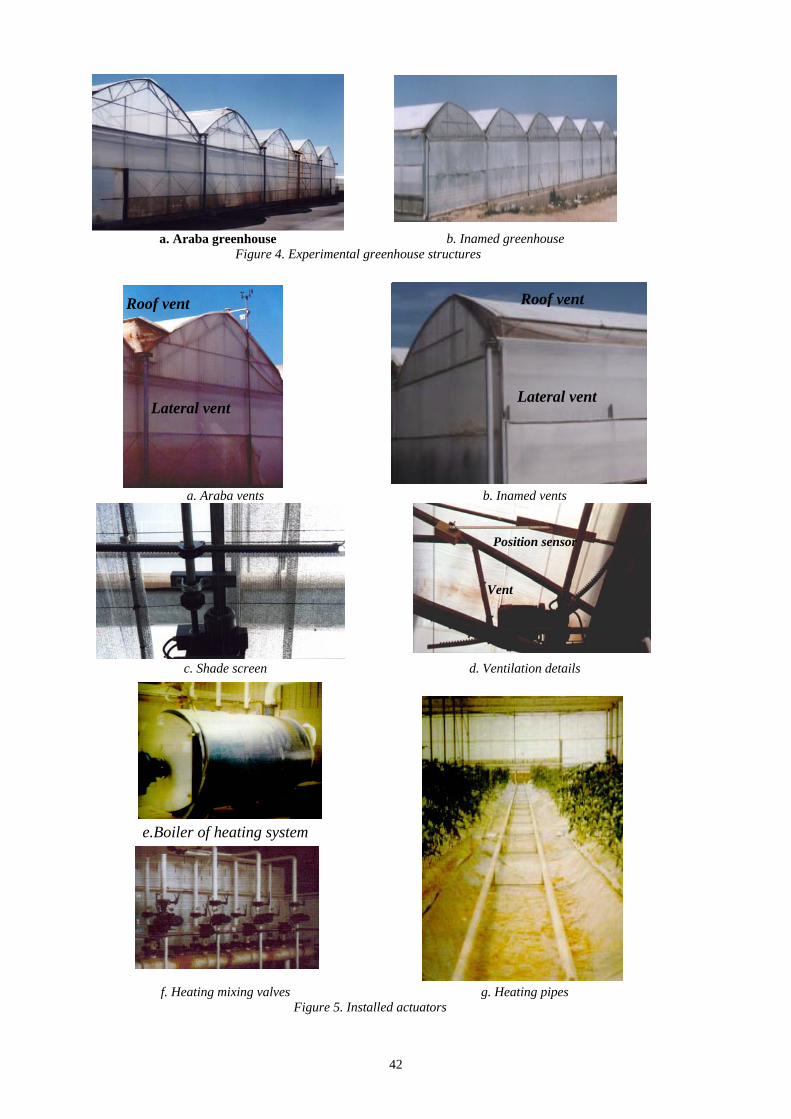
42

a. Araba greenhouse b. Inamed greenhouse Figure 4. Experimental greenhouse structures

a. Araba vents b. Inamed vents

c. Shade screen d. Ventilation details

e.Boiler of heating system

f. Heating mixing valves g. Heating pipes Figure 5. Installed actuators

Ventilación

Ventilación lateral

Roof vent

Lateral vent

Ventilación

Ventilación

Roof vent

Lateral vent

Sensoposició

Motor ventilació

Position sensor

Vent

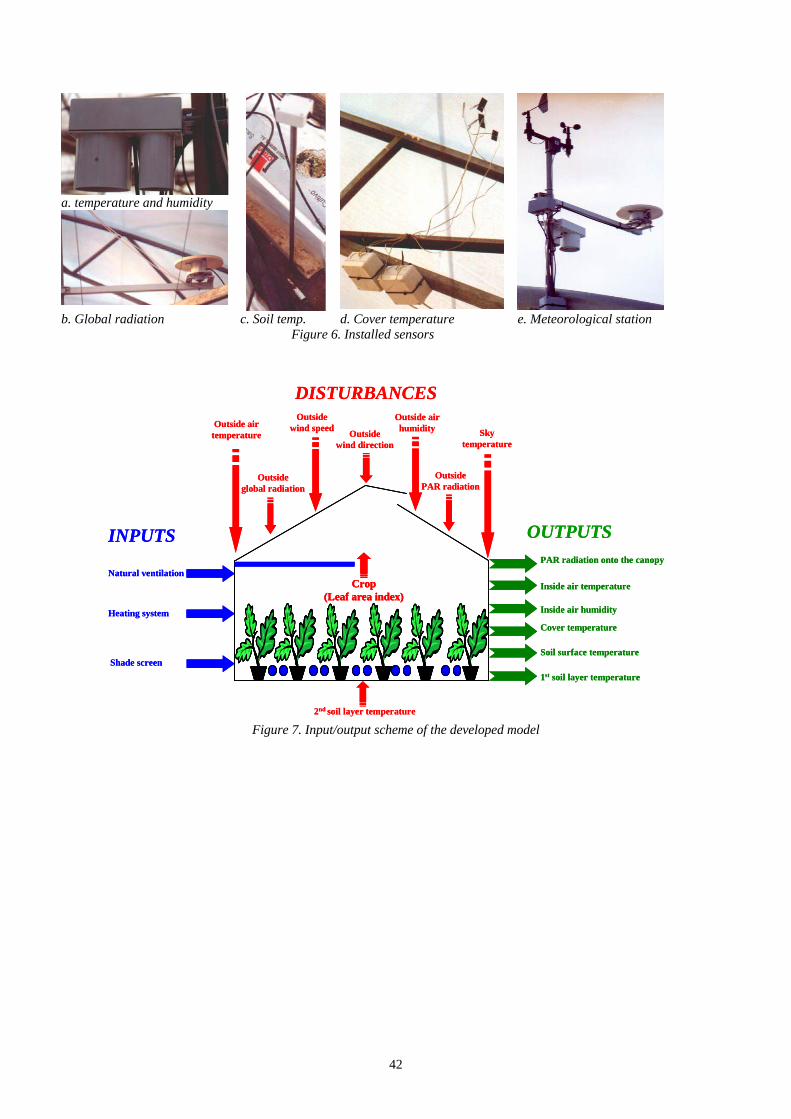
42

a. temperature and humidity

b. Global radiation c. Soil temp. d. Cover temperature e. Meteorological station

Figure 6. Installed sensors

Figure 7. Input/output scheme of the developed model

Inside air temperature

PAR radiation onto the canopy

Inside air humidity

Natural ventilation

Heating system

Shade screen

Outside airtemperature

Outsideglobal radiation

Outsidewind speed

Outsidewind direction

Outside airhumidity

DISTURBANCES

INPUTS OUTPUTS

2nd soil layer temperature

Skytemperature

Soil surface temperature

Cover temperature

1st soil layer temperature

Crop(Leaf area index)

OutsidePAR radiation


PAR radiation onto the canopy

Inside air humidity

Natural ventilation

Heating system

Shade screen

Outside airtemperature

Outsideglobal radiation

Outsidewind speed

Outsidewind direction

Outside airhumidity

DISTURBANCES

INPUTS OUTPUTS

2nd soil layer temperature

Skytemperature


Cover temperature

1st soil layer temperature



OutsidePAR radiation

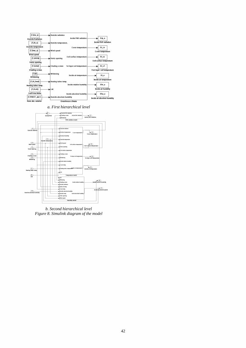
42

a. First hierarchical level

b. Second hierarchical level Figure 8. Simulink diagram of the model

[T,Dws_e]

W ind speed

C wh

W hitening

[T,UVEN]

Vents opening

Xt_ss


[T,Ushd]

Shading screen

[T,Dt_e]

Outside temperature

[T,Dre_e]

Outside Radiation

[T,VLA I]

Leaf A rea Index

Xt_a


Xhr_a

Inside air humidity

Xha_a

Inside air absolute humidity

Xrp_a

Inside PA R radiation

[T,PHEXT_abs']

Hum. abs. exterior

[T,Ut_heat]

Heating tubes temp.

Outsid e rad iatio n

Outsid e temp eratu re.

W in d speed

Vents o pen in g

S hading screen

W hiten ing

Heating tu bes temp .

L AI

Outsid e abso lu te hu mid ity

in side PAR rad iatio n

Cover temp erature

S oil surface temperature

1st layer so il temp erature

I nsid e air temp erature

I n side relative hu mid ity

I nsid e abso lu te hu mid ity

Greenhouse climate

Xt_s1

Fisrt layer soil temperature

Xt_cv

C over temperature

7Inside absolute hum idit

6Inside relative hum idity

5Inside air tem perature

41st layer soil tem perature

3Soil surface tem perature

2Cover tem perature

1inside PAR radiation

Outside radiation


Inside air humidity

Outside temperature

W ind speed

Vents opening


Shading screen

W hitening

Inside relative humidity

C over temp.

Heating tubes temperature

LA I

C over temperature1

Soil surface temperature1

1st layer soil temperature

Inside air temperature1

Tem perature m odel

Outside PA R radiation

S hading screen

W hitening

Inside PA R radiation

PAR radiation m odel

LA I

W hitening

S hading screen

Outside radiation

Inside air temp.

C over temp.

Outside absolute humidity

Outside temp.

V ents opening

W ind speed

Inside relative humidity

Inside absolute humidity

Hum idity m odel

0.

Global/PAR

9Outside absolute hum idity

8LAI

7Heating tubes tem p.

6Whitening

5Shading screen

4Vents opening

3Wind speed

2Outside tem perature.

1Outside radiation

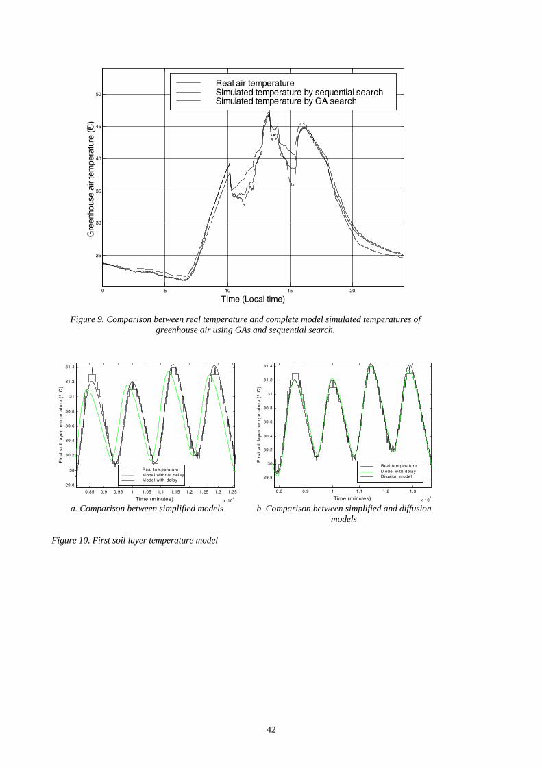
42

0 5 10 15 20

25

30

35

40

45

50G

reen

hous

e ai

r te

mpe

ratu

re (

ºC)

Time (Local time)

Real air temperatureSimulated temperature by sequential searchSimulated temperature by GA search

Figure 9. Comparison between real temperature and complete model simulated temperatures of

greenhouse air using GAs and sequential search.

0.85 0.9 0.95 1 1.05 1.1 1.15 1.2 1.25 1.3 1.35

x 104

29.8

30

30.2

30.4

30.6

30.8

31

31.2

31.4

Fir

st

so

il la

yer

tem

pe

ratu

re (

ºC

)

Time (minutes)

Real tem peratureModel without delayModel with delay

0.8 0.9 1 1.1 1.2 1.3

x 104

29.8

30

30.2

30.4

30.6

30.8

31

31.2

31.4

Time (minutes)

Fir

st

so

il la

yer

tem

pe

ratu

re (

ºC

)

Real tem peratureM odel with delayDifus ion m odel

a. Comparison between simplified models b. Comparison between simplified and diffusion

models

Figure 10. First soil layer temperature model

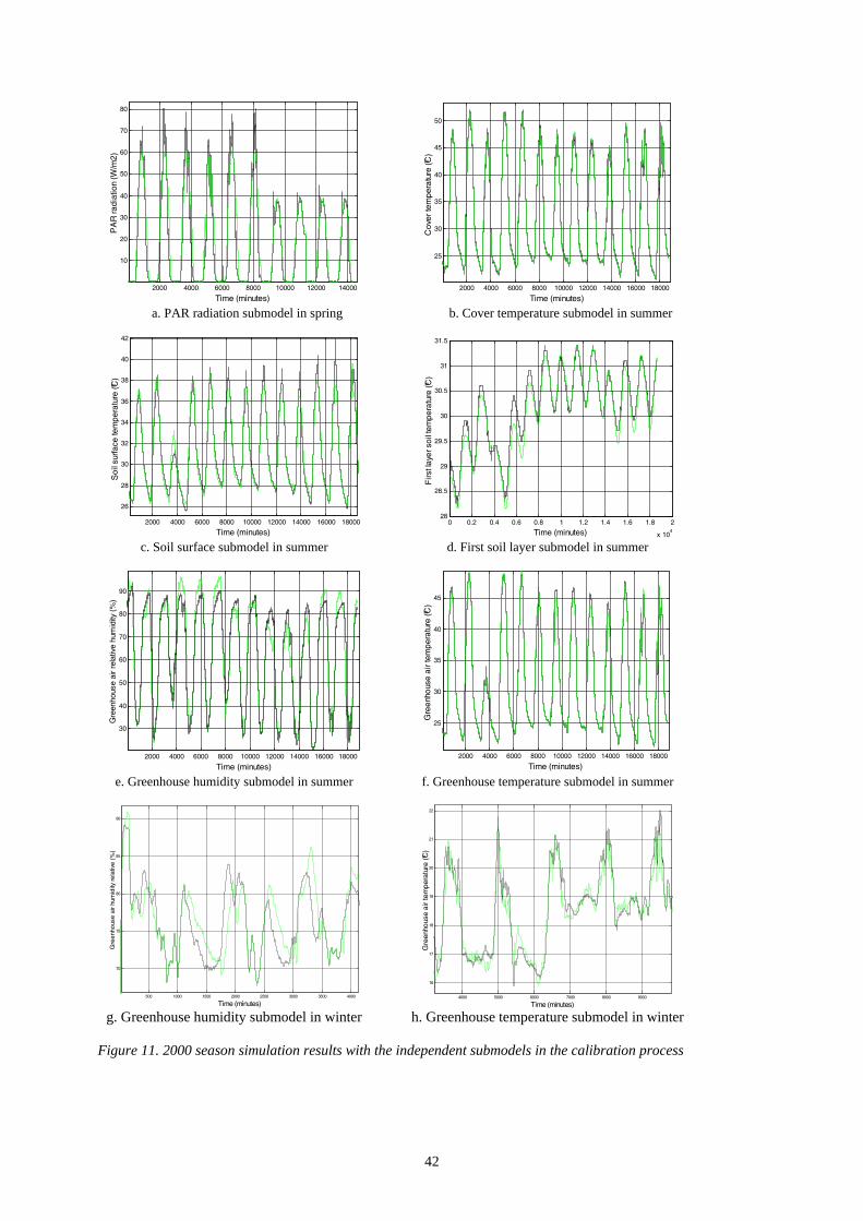
42

2000 4000 6000 8000 10000 12000 14000

10

20

30

40

50

60

70

80

Time (minutes)

PA

R ra

diat

ion

(W/m

2)

2000 4000 6000 8000 10000 12000 14000 16000 18000

25

30

35

40

45

50

Time (minutes)

Cov

er te

mpe

ratu

re (ºC

)

a. PAR radiation submodel in spring b. Cover temperature submodel in summer

2000 4000 6000 8000 10000 12000 14000 16000 18000

26

28

30

32

34

36

38

40

42

Soi

l sur

face

tem

pera

ture

(ºC)

Time (minutes) 0 0.2 0.4 0.6 0.8 1 1.2 1.4 1.6 1.8 2

x 104

28

28.5

29

29.5

30

30.5

31

31.5

Time (minutes)

Firs

t lay

er s

oil t

empe

ratu

re (ºC

)

c. Soil surface submodel in summer

d. First soil layer submodel in summer

2000 4000 6000 8000 10000 12000 14000 16000 18000

30

40

50

60

70

80

90

Time (minutes)

Gre

enho

use

air

rela

tive

hum

idity

(%

)

2000 4000 6000 8000 10000 12000 14000 16000 18000

25

30

35

40

45

Gre

enho

use

air t

empe

ratu

re (ºC

)

Time (minutes) e. Greenhouse humidity submodel in summer

f. Greenhouse temperature submodel in summer

500 1000 1500 2000 2500 3000 3500 4000

70

75

80

85

90

Time (minutes)

Gre

enho

use

air

hum

idity

rela

tive

(%)

4000 5000 6000 7000 8000 9000

16

17

18

19

20

21

22

Time (minutes)

Gre

enho

use

air

tem

pera

ture

(ºC

)

g. Greenhouse humidity submodel in winter

h. Greenhouse temperature submodel in winter

Figure 11. 2000 season simulation results with the independent submodels in the calibration process

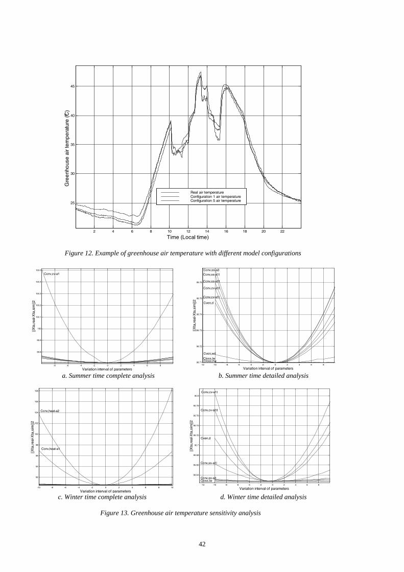
42

2 4 6 8 10 12 14 16 18 20 22

25

30

35

40

45

Time (Local time)

Gre

enh

ous

e a

ir te

mp

era

ture

(ºC

)

Real air temperatureConfiguration 1 air temperatureConfiguration 5 air temperature

Figure 12. Example of greenhouse air temperature with different model configurations

-8 -6 -4 -2 0 2 4 6 8

99.8

99.9

100

100.1

100.2

100.3

100.4

100.5

Variation interval of parameters

||Xta

,rea

l-Xta

,sim

||2

Ccnv,cv-a1

-12 -10 -8 -6 -4 -2 0 2 4 6 8

99.71

99.72

99.73

99.74

99.75

99.76

Ccnv,ss-a3Ccnv,ss-a1l

Ccnv,ss-a1t

Ccnv,cv-a1t

Ccnv,cv-a1l

Cven,d

Cven,wd

Closs,hwCloss,lw

||Xta

,rea

l-Xta

,sim

||2

Variation interval of parameters a. Summer time complete analysis

b. Summer time detailed analysis

-10 -8 -6 -4 -2 0 2 4 6 8 10

92

94

96

98

100

102

104

106

108


||Xta

,rea

l-Xta

,sim

||2

Ccnv,heat-a1

Ccnv,heat-a2

-12 -10 -8 -6 -4 -2 0 2 4 6 8

90.64

90.66

90.68

90.7

90.72

90.74

90.76

90.78

90.8


||Xta

,rea

l-Xta

,sim

||2

Ccnv,cv-a1t

Ccnv,cv-a1tl

Cven,d

Ccnv,ss-a1l

Ccnv,ss-a3Closs,lw

c. Winter time complete analysis d. Winter time detailed analysis

Figure 13. Greenhouse air temperature sensitivity analysis

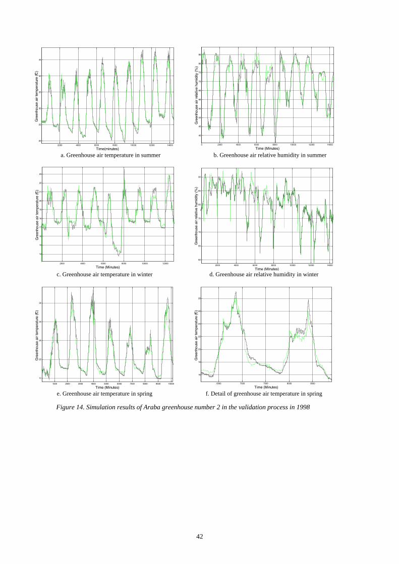
42

2000 4000 6000 8000 10000 12000 14000

20

25

30

35

40

45

Time(minutes)

Gre

enho

use

air

tem

pera

ture

(ºC

)

0 2000 4000 6000 8000 10000 12000 14000

40

45

50

55

60

65

70

75

80

85

Time (Minutes)

Gre

enho

use

air

rela

tive

hum

idity

(%

)

a. Greenhouse air temperature in summer

b. Greenhouse air relative humidity in summer

2000 4000 6000 8000 10000 12000

14

15

16

17

18

19

20

21

22

23

Time (Minutes)

Gre

enho

use

air

tem

pera

ture

(ºC

)

2000 4000 6000 8000 10000 12000 14000

60

65

70

75

80

85

90

Time (Minutes)

Gre

enho

use

air

rela

tive

hum

idity

(%

)

c. Greenhouse air temperature in winter

d. Greenhouse air relative humidity in winter

1000 2000 3000 4000 5000 6000 7000 8000 9000 10000

15

20

25

30

35

Time (Minutes)

Gre

enho

use

air

tem

pera

ture

(ºC

)

6500 7000 7500 8000 8500

16

18

20

22

24

26

28

Time (Minutes)

Gre

enho

use

air

tem

pera

ture

(ºC

)

e. Greenhouse air temperature in spring

f. Detail of greenhouse air temperature in spring

Figure 14. Simulation results of Araba greenhouse number 2 in the validation process in 1998

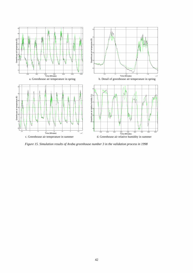
42

2000 4000 6000 8000 10000 12000 14000

12

14

16

18

20

22

24

26

28

Time (Minutes)

Gre

enho

use

air

tem

pera

ture

(ºC

)

1.35 1.4 1.45 1.5 1.55

x 104

25

30

35

40

45

50

Gre

enho

use

air

tem

pera

ture

(ºC

)

Time (Minutes) a. Greenhouse air temperature in spring

b. Detail of greenhouse air temperature in spring

0.8 1 1.2 1.4 1.6 1.8 2 2.2

x 104

20

25

30

35

40

45

50

Time (Minutes)

Gre

enho

use

air

tem

pera

ture

(ºC

)

1000 2000 3000 4000 5000 6000 7000 8000 9000

30

40

50

60

70

80

90

Time (Minutes)

Gre

enho

use

air

rela

tive

hum

idity

(%

)

c. Greenhouse air temperature in summer

d. Greenhouse air relative humidity in summer

Figure 15. Simulation results of Araba greenhouse number 3 in the validation process in 1998

42

2000 4000 6000 8000 10000 12000 14000

16

18

20

22

24

26

28

30

32

Time (Minutes)

Gre

enho

use

air

tem

pera

ture

(ºC

)

1.05 1.1 1.15 1.2 1.25 1.3 1.35 1.4 1.45

x 104

22

24

26

28

30

32

34

36

38

40

42

Gre

enho

use

air

tem

pera

ture

(ºC

)

Time (Minutes) a. Greenhouse air temperature in spring b. Detail of greenhouse air temperature in spring

0 2000 4000 6000 8000 10000 12000 14000 16000 1800015

20

25

30

35

40

45

Time (Minutes)

Gre

enho

use

air

tem

pera

ture

(ºC

)

1000 2000 3000 4000 5000 6000 7000 8000 9000 10000 11000

65

70

75

80

85

90

Time (Minutes)

Gre

enho

use

air

rela

tive

hum

idity

(%

)

c. Greenhouse air temperature in summer

d. Greenhouse air relative humidity in summer

Figure 16. Simulation results of Inamed greenhouse number 1 in the validation process in 1998

42

Air temperature

Cover temperature


First soil layer temperature

Air relative humidity

Sec. GA Sec. GA Sec. GA Sec. GA Sec. GA

Mean 1.13 0.93 0.89 0.79 0.74 0.64 0.34 0.32 4.29 3.92

Maximum 5.15 4.63 5.17 4.81 4.66 4.65 1.36 1.26 29.47 24.32 Standard deviation

0.88 0.65 0.79 0.64 0.63 0.50 0.28 0.26 3.76 3.69

Table 1. Comparison between real temperature (ºC) and relative humidity (%) and the estimation of the compound model using GAs and direct sequential search during August 2000

Summer 2000 Winter 2000 Air

temperature Air relative humidity

Cover temperature


First soil layer temperature

Air temperature

Air relative humidity

Variation interval

21.1-49.0 (27.9 ºC)

21-94 (73 %)

20.55-52.1 (31.55 ºC)

25.5-42 (16.5 ºC)

28.19-31.4 (5.9 ºC)

11.5-25.5 (14 ºC)

49.7-100 (50.3 %)

Mean 0.51 3.96 0.52 0.68 0.25 0.52 2.53

Maximum 2.81 24.32 3.38 4.12 0.79 2.06 17.19 Standard deviation

0.52 3.75 0.53 0.44 0.17 0.48 2.39

Table 2. Comparative results of the estimation of the different climate variables in the calibration process

Configuration 1 Configuration 2 Configuration 3 Configuration 4 Configuration 5

Mean 0.51 0.52 0.61 0.93 0.95

Maximum 2.81 2.83 3.12 4.63 4.73 Standard deviation

0.52 0.53 0.59 0.65 0.66

Table 3. Comparative results of the estimation of the greenhouse air temperature using different configurations under summer 2000 conditions (ºC)

January 1998 April 1998 August 1998

Temperature Humidity Temperature Humidity Temperature Humidity

Variation interval

13.76-23.55 (9.79 ºC)

55.64-100 (44.36 %)

14.5-38.6

(24.1 ºC) 58.95-92.05

(33.1 %) 19.4-48.6 (29.2 ºC)

36.36-87.47 (51.11 %)

Mean 0.63 3.04 0.95 2.12 0.77 2.56

Maximum 3.02 19.61 5.5 11.74 4.07 17.46 Standard deviation

0.51 2.98 1.1 2.67 0.64 2.31

Table 4. Comparative results of the estimation of the different climate variables in Araba greenhouse number 2 in the validation process

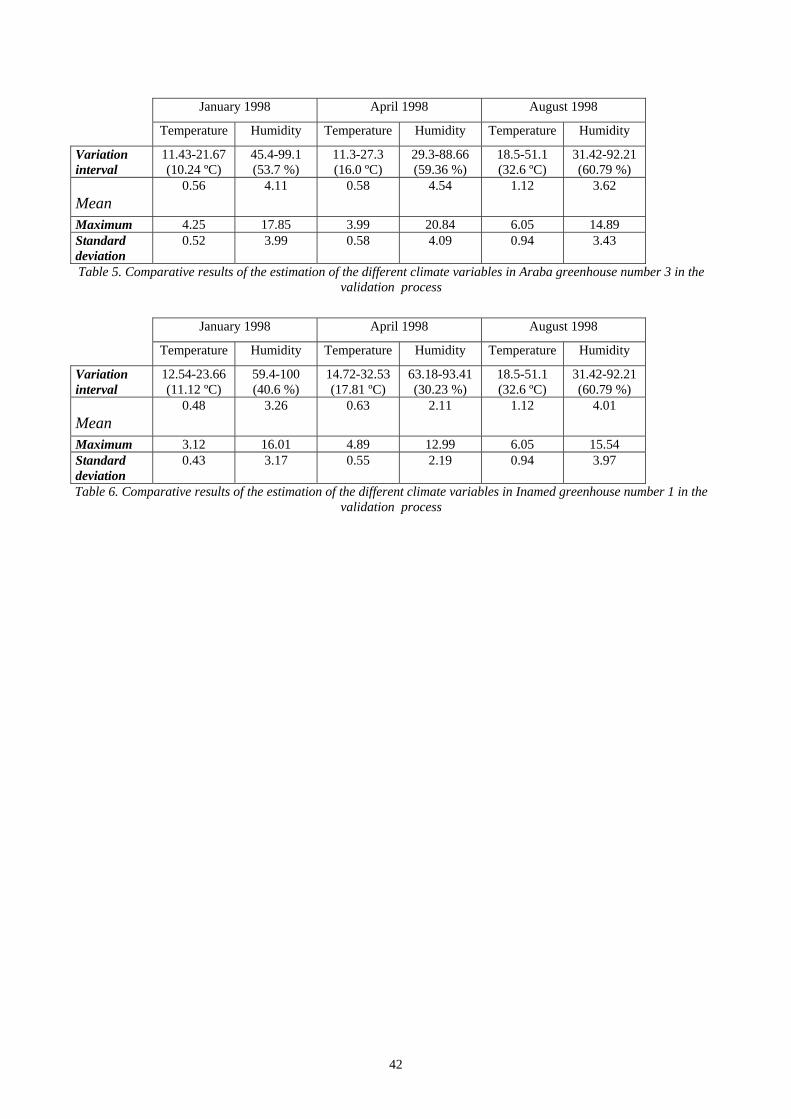
42



Variation interval

11.43-21.67 (10.24 ºC)

45.4-99.1 (53.7 %)

11.3-27.3 (16.0 ºC)

29.3-88.66 (59.36 %)

18.5-51.1 (32.6 ºC)

31.42-92.21 (60.79 %)

Mean 0.56 4.11 0.58 4.54 1.12 3.62


0.52 3.99 0.58 4.09 0.94 3.43

Table 5. Comparative results of the estimation of the different climate variables in Araba greenhouse number 3 in the validation process



Variation interval

12.54-23.66 (11.12 ºC)

59.4-100 (40.6 %)

14.72-32.53 (17.81 ºC)

63.18-93.41 (30.23 %)

18.5-51.1 (32.6 ºC)

31.42-92.21 (60.79 %)

Mean 0.48 3.26 0.63 2.11 1.12 4.01


0.43 3.17 0.55 2.19 0.94 3.97

Table 6. Comparative results of the estimation of the different climate variables in Inamed greenhouse number 1 in the validation process

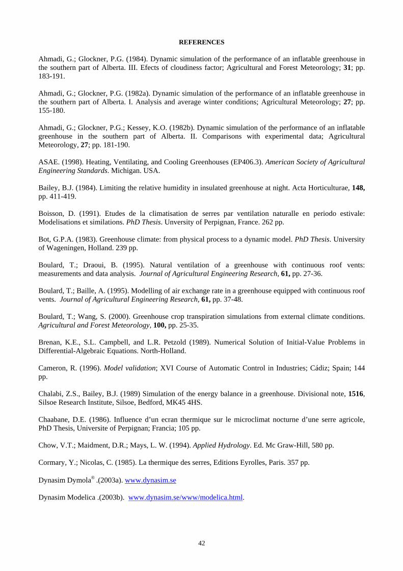
42

REFERENCES

Ahmadi, G.; Glockner, P.G. (1984). Dynamic simulation of the performance of an inflatable greenhouse in the southern part of Alberta. III. Efects of cloudiness factor; Agricultural and Forest Meteorology; 31; pp. 183-191. Ahmadi, G.; Glockner, P.G. (1982a). Dynamic simulation of the performance of an inflatable greenhouse in the southern part of Alberta. I. Analysis and average winter conditions; Agricultural Meteorology; 27; pp. 155-180. Ahmadi, G.; Glockner, P.G.; Kessey, K.O. (1982b). Dynamic simulation of the performance of an inflatable greenhouse in the southern part of Alberta. II. Comparisons with experimental data; Agricultural Meteorology, 27; pp. 181-190. ASAE. (1998). Heating, Ventilating, and Cooling Greenhouses (EP406.3). American Society of Agricultural Engineering Standards. Michigan. USA. Bailey, B.J. (1984). Limiting the relative humidity in insulated greenhouse at night. Acta Horticulturae, 148, pp. 411-419. Boisson, D. (1991). Etudes de la climatisation de serres par ventilation naturalle en periodo estivale: Modelisations et similations. PhD Thesis. Unversity of Perpignan, France. 262 pp. Bot, G.P.A. (1983). Greenhouse climate: from physical process to a dynamic model. PhD Thesis. University of Wageningen, Holland. 239 pp. Boulard, T.; Draoui, B. (1995). Natural ventilation of a greenhouse with continuous roof vents: measurements and data analysis. Journal of Agricultural Engineering Research, 61, pp. 27-36. Boulard, T.; Baille, A. (1995). Modelling of air exchange rate in a greenhouse equipped with continuous roof vents. Journal of Agricultural Engineering Research, 61, pp. 37-48. Boulard, T.; Wang, S. (2000). Greenhouse crop transpiration simulations from external climate conditions. Agricultural and Forest Meteorology, 100, pp. 25-35. Brenan, K.E., S.L. Campbell, and L.R. Petzold (1989). Numerical Solution of Initial-Value Problems in Differential-Algebraic Equations. North-Holland. Cameron, R. (1996). Model validation; XVI Course of Automatic Control in Industries; Cádiz; Spain; 144 pp. Chalabi, Z.S., Bailey, B.J. (1989) Simulation of the energy balance in a greenhouse. Divisional note, 1516, Silsoe Research Institute, Silsoe, Bedford, MK45 4HS. Chaabane, D.E. (1986). Influence d’un ecran thermique sur le microclimat nocturne d’une serre agricole, PhD Thesis, Universite of Perpignan; Francia; 105 pp. Chow, V.T.; Maidment, D.R.; Mays, L. W. (1994). Applied Hydrology. Ed. Mc Graw-Hill, 580 pp. Cormary, Y.; Nicolas, C. (1985). La thermique des serres, Editions Eyrolles, Paris. 357 pp. Dynasim Dymola .(2003a). www.dynasim.se Dynasim Modelica .(2003b). www.dynasim.se/www/modelica.html.

42

Garzoli, K.V.; Blackwell, J. (1981). An analysis of the nocturnal heat loss from a single skin plastic greenhouse, Journal of Agricultural Engineering Research, Vol. 26, pp. 203-214. Halleaux, D. (1989). Modele dynamique des échanges énergétiques des serres: étude théorique et expérimentale; PhD Thesis; Faculté des Sciencies Agronomiques de Gembloux; Belgium; 278 pp. van Henten, E.J. (1994). Greenhouse climate management: an optimal control approach; PhD Thesis; Agricultural University of Wageningen; Holland; 329 pp. Houck, C.; Joines. J.; Kay, M. (1995). The genetic algorithm for function optimization: a Matlab implementation; Technical report. Dept. Industrial Engineering. North Carolina State University. 14 pp. http://www.ie.ncsu.edu/mirage/GAToolBox/gaot/ Ioslovich, I.; Seginer, I.; Gutman, P.O.; Borshchevsky, M. (1995). Sub-optimal CO2 enrichment of greenhouses; Journal of Agricultural Engineering Research, Vol. 60, pp. 117-136. Jones, J.W. et al. (1991). A dynamic tomato growth and yield model (TOMGRO). Transactions of the ASAE, 34 (2), pp. 663-672. Kindelan, M. (1980). Dynamic modeling of greenhouse environment, Transactions of the ASAE, 23, pp. 1232-1239. Manera, C.; Picuno, P.; Scarascia, G. (1990). Analysis of nocturnal microclimate in a single skin cold greenhouse in Mediterranean countries, Acta Horticulturae, 281, pp. 47-56. Matous, K.; Leps, M.; Zeman, J.; Sejnoha, M. (2000). Applying genetic algorithm to selected topics commonly encountered in engineering practice. Computer methods in applied mechanics and engineering, 190, pp. 1629-1650. MathWorks Inc. (1998a). Using Matlab. The Lenguage of Technical Computing, USA, 531 pp. MathWorks Inc. (1998b). Using Simulink. Dynamic Systems Simulation for Matlab, USA, 645 pp. Montero, J.I.; Antón, A.; Muñoz, P. (1998). Refrigeración de invernaderos; Curso Superior de Especialización: Tecnología de Invernaderos II; Editado por la Dirección General de Investigación y Formación Agroalimentaria de la Junta de Andalucía, FIAPA y Caja Rural de Almería; 313-338 pp. Muñoz, P.; Montero, J.I.; Antón, A.; Giuffrida, F. (1998). Effect of insect-proof screens and roof openings on greenhouse ventilation; Journal of Agricultural Engineering Research; 73; pp. 171-178. Pearson, R.K. (1995). Nonlinear input/output modelling. J. Process Control, 5 (4), pp. 197-211. Rodríguez, F. (2002). Modelado y control jerárquico de crecimiento de cultivo en invernaderos. PhD Thesis, University of Almería, Spain, 365 pp. Rodríguez, F., Yebra, L., Berenguel, M., Dormido, S. (2002). Modeling and simulation of greenhouse climate using Dymola. 15th IFAC World Congress, Barcelona, Spain; 6 pp. Rumbaugh, J., Blaha, M.; Premerlani, W.; Eddy, F.; Lorensen, W. (1991). Object-Oriented Modeling and Design. Prentice Hall. Sahin, Ö; Sayan, P.; Buluctu, A.N. (2000). Application of genetic algorithms for determination of mass transfer coefficients; Journal of Crystal growth; 216, pp. 475-482. Seginer, I. (1997). Alternative design formulae for the ventilation rate of greenhouse. Journal of Agricultural Engineering Research, 68, pp. 355-365.

42

Senent, J.S.; Martínez, M.A.; Blasco, X.; Sanchís, J. (1998). MIMO predictive control of temperature and humidity inside a greenhouse using Simulated Annealing (SA) as optimiser of a multicriteria index; 11th International Conference on Industrial & Engineering Applications of Artificial Intelligence & Expert Systems; Castellón, Spain; 9 pp. Sharme, P.K.; Tiwari; G.N.; Sorayan, V.P.S. (1999). Temperature distribution in different zones of the microclimate of a greenhouse: a dynamic model; Energy Conversion & Management; Vol. 40; pp. 335-348. Stanghellini, C. (1987). Transpiration of greenhouse crops, IMAG Publication, Wageningen, Holland, 150 pp Stanghellini, C., de Jong, T. (1995). A model of humidity and its applications in a greenhouse. Agricultural and Forest Meteorology, 76, pp. 120-148. Takakura, T. (1993). Climate under cover; Kluwer Academic Publishers; Holanda; 155 pp. Takakura, T.; Jordan, K.A.; Boyd, L.L. (1971). Dynamic simulation of plant growth and environment in the greenhouse; Transactions of the ASAE; N. 5; pp. 964-971. Tap, F. (2000). Economised-based optimal control of greenhouse tomato crop production; PhD Thesis; Agricultural University of Wageningen; Holland; 127 pp. Tap, F.; van Willigenburg, L.G.; van Straten, G. (1996a). Experimental results of receding horizon optimal control of greenhouse climate; Acta Horticulturae; 406; pp. 229-238. Tap, F.; van Willigenburg, L.G.; van Straten, G. (1996b). Receding horizon optimal control of greenhouse climate based on the lazy man weather prediction; 13th IFAC World Congress; San Francisco; USA; pp. 387-392. Tavares, C.; Gonzalves, A.; Castro, P.; Loureiro, D.; Joyce, A. (2001). Modelling an agriculture production greenhouse; Renewable energy; Vol. 22; pp. 15-20. Tchamitchian, M.; Tantau, H.J. (1996). Optimal control of the daily greenhouse climate: physical approach; 13th IFAC World Congress; San Francisco; USA; pp. 471-475. Tchamitchian, M.; van Willigenburg, L.G.; van Straten, G. (1993). Optimal control applied to tomato crop production in a greenhouse; European Control Conference; Groningen; Holland, Vol. 3; pp. 1348-324. Trigui, M.; Barrington, S.; Gauthier, L. (2001a). A strategy for greenhouse climate control, Part I: Model development; Journal of Agricultural Engineering Research; Vol. 78 (4); pp. 407-423. Trigui, M.; Barrington, S.; Gauthier, L. (2001b). A strategy for greenhouse climate control, Part II: Model validation; Journal of Agricultural Engineering Research; Vol. 79 (1); pp. 99-105. Udink ten Cate, A.J. (1983). Modeling and (adaptive) control of greenhouse climates; PhD Thesis; Agricultural University of Wageningen; Holland; 159 pp. Wang, S; Boulard, T. (2000). Predicting the microclimate in a naturally ventilated plastic house in a Mediterranean climate; Journal of Agricultural Engineering Research, N. 75, pp. 27-38. Wang, S; Boulard, T.; Haxaire, R. (1999). Air speed profiles in a naturally ventilated greenhouse with a tomato crop. Agricultural and Forest Meteorology, 96, pp. 181-188. Wang, Q.J. (1997). Using genetic algorithms to optimise model parameters; Environmental modelling & software; Volume 12, N. 1, pp.27-34.

42

Young, P.; Lees, M.; Chotai, A.; Tych, W. (1993). The modelling and multivariable control of glasshouse systems; 12th IFAC World Congress; Sidney; Australia; Vol. 10; pp. 313-316. Zhang, Y.; Mahrer, Y.; Margolin, M. (1997). Predicting the microclimate inside a greenhouse: an application of a one-dimensional numerical model in an unheated greenhouse; Agricultural and Forest Meteorology, N. 86, pp. 291-297.

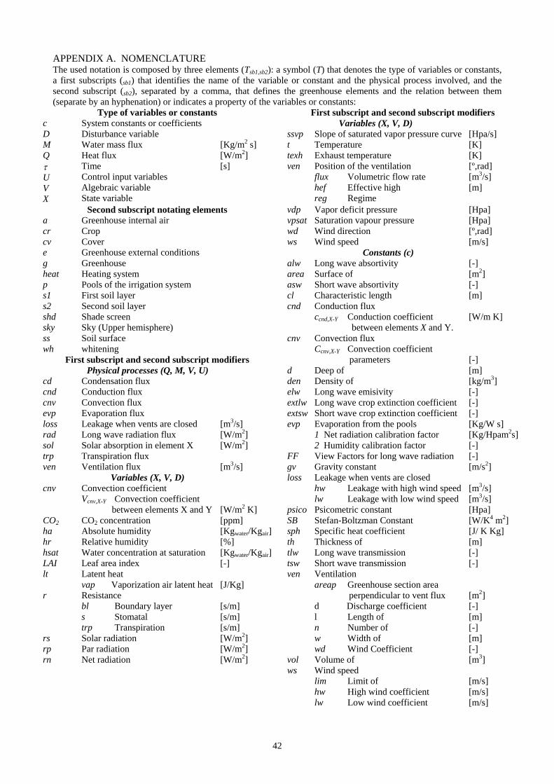
42

APPENDIX A. NOMENCLATURE The used notation is composed by three elements (Tsb1,sb2): a symbol (T) that denotes the type of variables or constants, a first subscripts (sb1) that identifies the name of the variable or constant and the physical process involved, and the second subscript (sb2), separated by a comma, that defines the greenhouse elements and the relation between them (separate by an hyphenation) or indicates a property of the variables or constants:

Type of variables or constants First subscript and second subscript modifiers c D M Q U V X

System constants or coefficients Disturbance variable Water mass flux Heat flux Time Control input variables Algebraic variable State variable

[Kg/m2 s] [W/m2] [s]

ssvp t texh ven

Variables (X, V, D) Slope of saturated vapor pressure curveTemperature Exhaust temperature Position of the ventilation flux Volumetric flow rate hef Effective high reg Regime

[Hpa/s] [K] [K] [º,rad] [m3/s] [m]

Second subscript notating elements vdp Vapor deficit pressure [Hpa] a cr cv e g heat p s1 s2 shd sky ss wh

Greenhouse internal air Crop Cover Greenhouse external conditions Greenhouse Heating system Pools of the irrigation system First soil layer Second soil layer Shade screen Sky (Upper hemisphere) Soil surface whitening

vpsatwd ws alw area asw cl cnd cnv

Saturation vapour pressure Wind direction Wind speed

Constants (c) Long wave absortivity Surface of Short wave absortivity Characteristic length Conduction flux ccnd,X-Y Conduction coefficient between elements X and Y. Convection flux Ccnv,X-Y Convection coefficient

[Hpa] [º,rad] [m/s] [-] [m2] [-] [m] [W/m K]

First subscript and second subscript modifiers parameters [-] cd cnd cnv evp loss rad sol trp ven cnv CO2 ha hr hsat LAI lt r rs rp rn

Physical processes (Q, M, V, U) Condensation flux Conduction flux Convection flux Evaporation flux Leakage when vents are closed Long wave radiation flux Solar absorption in element X Transpiration flux Ventilation flux

Variables (X, V, D) Convection coefficient Vcnv,X-Y Convection coefficient between elements X and Y CO2 concentration Absolute humidity Relative humidity Water concentration at saturation Leaf area index Latent heat

vap Vaporization air latent heat Resistance bl Boundary layer s Stomatal trp Transpiration Solar radiation Par radiation Net radiation

[m3/s] [W/m2] [W/m2] [m3/s] [W/m2 K] [ppm] [Kgwater/Kgair][%] [Kgwater/Kgair][-] [J/Kg] [s/m] [s/m] [s/m] [W/m2] [W/m2] [W/m2]

d den elw extlwextswevp FF gv loss psicoSB sph th tlw tsw ven vol ws

Deep of Density of Long wave emisivity Long wave crop extinction coefficient Short wave crop extinction coefficient Evaporation from the pools 1 Net radiation calibration factor 2 Humidity calibration factor View Factors for long wave radiation Gravity constant Leakage when vents are closed hw Leakage with high wind speedlw Leakage with low wind speed Psicometric constant Stefan-Boltzman Constant Specific heat coefficient Thickness of Long wave transmission Short wave transmission Ventilation areap Greenhouse section area

perpendicular to vent flux d Discharge coefficient l Length of n Number of w Width of wd Wind Coefficient Volume of Wind speed lim Limit of hw High wind coefficient lw Low wind coefficient

[m] [kg/m3] [-] [-] [-] [Kg/W s] [Kg/Hpam2s][-] [-] [m/s2] [m3/s] [m3/s] [Hpa] [W/K4 m2] [J/ K Kg] [m] [-] [-] [m2] [-] [m] [-] [m] [-] [m3] [m/s] [m/s] [m/s]

design, implementation, calibration and validation of...

Documents