design, implementation and evaluation of a redundancy
TRANSCRIPT

Western University Western University
Scholarship@Western Scholarship@Western
Electronic Thesis and Dissertation Repository
4-15-2019 3:30 PM
Design, Implementation and Evaluation of a Redundancy Design, Implementation and Evaluation of a Redundancy
Management System for Fault-Tolerant Wireless Devices in Harsh Management System for Fault-Tolerant Wireless Devices in Harsh
Environments Environments
Madison McCarthy, The University of Western Ontario
Supervisor: Jiang, Jin, The University of Western Ontario
A thesis submitted in partial fulfillment of the requirements for the Master of Engineering
Science degree in Electrical and Computer Engineering
© Madison McCarthy 2019
Follow this and additional works at: https://ir.lib.uwo.ca/etd
Part of the Electrical and Electronics Commons
Recommended Citation Recommended Citation McCarthy, Madison, "Design, Implementation and Evaluation of a Redundancy Management System for Fault-Tolerant Wireless Devices in Harsh Environments" (2019). Electronic Thesis and Dissertation Repository. 6149. https://ir.lib.uwo.ca/etd/6149
This Dissertation/Thesis is brought to you for free and open access by Scholarship@Western. It has been accepted for inclusion in Electronic Thesis and Dissertation Repository by an authorized administrator of Scholarship@Western. For more information, please contact [email protected].

ii
Abstract
Wireless sensor networks (WSNs), when deployed in harsh environments, can fail prematurely
due to elevated rates of component failures. To counteract this problem, fault-tolerant
techniques, such as redundancy, may be used. A redundant design requires a management
system. Built-in tests (BITs) are one of the most commonly used approaches for managing
redundancy, but it suffers from issues such as imperfect fault coverage and common-cause
failures (CCFs). In this work, a BIT based redundancy management system has been designed
that makes use of a supervisory unit and a modular architecture to address issues with imperfect
fault coverage and CCFs. The design has been implemented in prototype WSN devices and
evaluated through reliability analysis, fault injection testing and industrial test deployments.
The evaluation results have demonstrated the fault-tolerant capabilities of the proposed system
design.
Keywords
Wireless Sensor Network (WSN), Fault-Tolerant, Built-in Tests (BITs), Redundancy
Management System, Common-Cause Failure (CCF), Fault Coverage.

iii
Acknowledgments
I would like to express my gratitude towards my supervisor, Dr. Jin Jiang, for being supportive
and understanding during my endeavors as a graduate student. He stands as an inspiration due
to his dedication to research excellence and I am thankful to have had the opportunity to learn
and grow under his guidance. I would also like to thank Dr. Ataul Bari for his patience and
encouragement throughout my research. Without his support or technical expertise, my work
would have little resemblance to its current form. As well, Dr. Xinhong Huang has been an
invaluable resource during my studies and has guided me to completion during the most
difficult months.
A special thank you is needed for Dr. Dennis Michaelson. His willingness to always provide
sound advice has had a resounding impact on my research. His vast knowledge with electronics
has significantly shortened the time to realize my design and has helped to give me a broader
perspective towards engineering.
Further, I would like to recognize the University Network of Excellence in Nuclear
Engineering (UNENE), Ontario Power Generation (OPG), and Bruce Power for providing their
facilities to learn and financial assistance that made this research possible.

iv
Table of Contents
Abstract ............................................................................................................................... ii
Acknowledgments.............................................................................................................. iii
Table of Contents ............................................................................................................... iv
List of Tables .................................................................................................................... vii
List of Figures .................................................................................................................. viii
List of Symbols .................................................................................................................. xi
List of Abbreviations ....................................................................................................... xiv
Chapter 1 ............................................................................................................................. 1
1 Introduction .................................................................................................................... 1
1.1 WSNs in Harsh Environments ................................................................................ 2
1.2 Redundant WSN Design ......................................................................................... 3
1.3 Issues with Built-in Tests ........................................................................................ 6
1.4 Research Objectives, Scope and Methods .............................................................. 6
1.4.1 Research Objectives .................................................................................... 6
1.4.2 Research Scope ........................................................................................... 7
1.4.3 Methods....................................................................................................... 7
1.5 Organization ............................................................................................................ 8
Chapter 2 ............................................................................................................................. 9
2 Background & Literature Review .................................................................................. 9
2.1 Fault-Tolerant Systems ........................................................................................... 9
2.1.1 Principles and Evaluation Metrics .............................................................. 9
2.1.2 Impact of Harsh Environments on Electronic Components ..................... 12

v
2.1.3 Redundancy Management Systems Using the BIT Approach .................. 15
2.2 WSNs for Harsh Environments ............................................................................ 16
2.2.1 Device-Level Architecture ........................................................................ 16
2.2.2 Existing Monitoring Systems in Harsh Environments.............................. 18
2.3 Limitations of Existing Work ............................................................................... 18
Chapter 3 ........................................................................................................................... 21
3 Modelling Imperfect Fault Coverage ........................................................................... 21
3.1 Modelling Imperfect Fault Coverage Without CCFs............................................ 21
3.2 Modelling Imperfect Fault Coverage with CCFs.................................................. 30
3.3 Impact of Modularity on CCFs ............................................................................. 38
3.4 Impact of Diversity in Design on CCFs ................................................................ 45
3.5 Summary of Considerations .................................................................................. 45
Chapter 4 ........................................................................................................................... 46
4 Redundancy Management System Design ................................................................... 46
4.1 Device Topology ................................................................................................... 46
4.2 Microcontroller-Based Built-in Test ..................................................................... 47
4.3 Supervisory Diagnostic Algorithm ....................................................................... 48
4.4 Supplementary Fault Detection Hardware ............................................................ 50
4.5 Design Summary ................................................................................................... 50
Chapter 5 ........................................................................................................................... 51
5 WSN Implementation................................................................................................... 51
5.1 Hardware Implementation .................................................................................... 51
5.1.1 Diverse Component Selection................................................................... 51
5.1.2 Circuit Simulations ................................................................................... 53
vi
5.1.3 PCB Modules ............................................................................................ 57
5.2 Software Implementation ...................................................................................... 61
5.2.1 Hardware Drivers ...................................................................................... 63
5.2.2 Operating System Porting ......................................................................... 63
5.2.3 MAC and Network Layers ........................................................................ 64
5.2.4 Application Layer ..................................................................................... 65
5.2.5 Remote Server Integration ........................................................................ 65
5.3 Implementation Summary ..................................................................................... 65
Chapter 6 ........................................................................................................................... 67
6 Redundancy Management System Evaluation ............................................................. 67
6.1 Reliability Analysis ............................................................................................... 67
6.2 Fault Injection Testing .......................................................................................... 71
6.3 WSN Experimental Test Scenarios ....................................................................... 76
6.3.1 Test Scenario #1: One-Module Data Trending ......................................... 77
6.3.2 Test Scenario #2: Two-Module Data Trending ........................................ 78
6.4 Evaluation Summary ............................................................................................. 80
Chapter 7 ........................................................................................................................... 82
7 Conclusions .................................................................................................................. 82
7.1 Summary ............................................................................................................... 82
7.2 Contributions......................................................................................................... 82
7.3 Conclusions ........................................................................................................... 83
7.4 Suggestions for Future Work ................................................................................ 83
References ......................................................................................................................... 85
Curriculum Vitae .............................................................................................................. 89

vii
List of Tables
Table 5.1: Diverse component selection. ................................................................................ 52
Table 5.2: Developed microcontroller drivers. ....................................................................... 63
Table 5.3: Summary of porting requirements for RIOT OS. .................................................. 64
Table 6.1: Environment within a NPP during normal (N) and accident (A) conditions. ....... 68
Table 6.2: Failure rates and scaling factors for various components. ..................................... 68
Table 6.3: Results of the fault coverage fault injection tests. ................................................. 74
Table 6.4: Results of the CCF fault injection tests. ................................................................ 75
Table 6.5: Event loss rate results for test scenario #1. ............................................................ 78
Table 6.6: Event loss rate results for test #2. .......................................................................... 80

viii
List of Figures
Figure 1.1: Topology of a WSN. .............................................................................................. 2
Figure 1.2: BIT approach for redundant components. .............................................................. 4
Figure 1.3: Voting logic approach for redundant components. ................................................ 5
Figure 2.1: Example of a reliability block diagram for a WSN gateway device. ................... 11
Figure 2.2: Fault tree for three WSN devices. ........................................................................ 12
Figure 2.3: Redundancy management with BITs and comparison logic. ............................... 16
Figure 2.4: Typical components of a WSN field device. ........................................................ 17
Figure 2.5: Typical components of a WSN gateway device. .................................................. 17
Figure 3.1: System reliability under imperfect fault coverage. .............................................. 24
Figure 3.2: Redundancy-relevance boundary for a BIT-based system. .................................. 25
Figure 3.3: Modified BIT topology to include a supervisory unit. ......................................... 26
Figure 3.4: Bounding effect of the coverage decay function. ................................................. 29
Figure 3.5: Redundancy-relevance boundary for both redundancy approaches. .................... 32
Figure 3.6: Advanced redundancy-relevance boundary considering imperfect fault coverage
and CCFs. ................................................................................................................................ 33
Figure 3.7: Reliability-improvement planes for different levels of redundancy. ................... 35
Figure 3.8: Reliability-improvement plane for a supervisory unit system under a varying 𝛾
and 𝛽𝑠-factor. .......................................................................................................................... 37

ix
Figure 3.9: Modularized dual-redundant system topology. .................................................... 38
Figure 3.10: Quadruple-redundant system using voting logic. ............................................... 39
Figure 3.11: Comparison of reliability for different topologies. ............................................ 41
Figure 3.12: Reliability-improvement plane for the dual-redundant system versus the
modularized system with γ=1. ................................................................................................ 43
Figure 3.13: Reliability-improvement plane for the dual-redundant system versus the
modularized system with γ=0.1. ............................................................................................. 44
Figure 4.1: Proposed redundancy management system topology. .......................................... 46
Figure 4.2: Features of the supervisory diagnostic algorithm................................................. 49
Figure 5.1: Sensor interface schematic. .................................................................................. 54
Figure 5.2: Sensor interface simulation results. ...................................................................... 54
Figure 5.3: CC1310 filtering schematic. (Left, TX) (Right, RX). .......................................... 55
Figure 5.4: CC1310 filtering simulation. (Left, TX) (Right, RX). ......................................... 55
Figure 5.5: EZR32LG filtering schematic. (Left TX) (Right RX). ........................................ 56
Figure 5.6: EZR32LG filtering simulation. (Left TX) (Right RX). ........................................ 56
Figure 5.7: Circuit simulation depicting a trip signal for the fault detection hardware. ......... 57
Figure 5.8: Module A PCB prototype. .................................................................................... 58
Figure 5.9: Module B PCB prototype. .................................................................................... 58
Figure 5.10: Sub-modules A1 (left) and A2 (right). ............................................................... 59
Figure 5.11: Sub-modules B1 (left) and B2 (right)................................................................. 59

x
Figure 5.12: Sub-modules S1 (left) and S2 (right). ................................................................ 60
Figure 5.13: Sub-modules AUX1 (left) and AUX2 (right)..................................................... 60
Figure 5.14: Proprietary fault detection hardware sub-module. ............................................. 61
Figure 5.15: Modularized design. ........................................................................................... 61
Figure 5.16: Software stack for implementation..................................................................... 62
Figure 6.1: IRIS mote (left) and the Meshlium gateway (right) device. ................................. 69
Figure 6.2: Reliability comparison for different devices under elevated environmental
conditions (105oC). ................................................................................................................. 70
Figure 6.3: Reliability comparison for different devices under elevated environmental
conditions (165oC). ................................................................................................................. 70
Figure 6.4: Method for injecting faults into a device. ............................................................. 71
Figure 6.5: Fault injection test scenario. ................................................................................. 72
Figure 6.6: Nuclear Plant Control Test Facility. ..................................................................... 76
Figure 6.7: A one-module device interfaced to the NPCTF. .................................................. 77
Figure 6.8: Test scenario #1 setup. ......................................................................................... 77
Figure 6.9: Test scenario #1 ThingSpeak server results. ........................................................ 78
Figure 6.10: Interfacing of the two-module device. ............................................................... 79
Figure 6.11: Test scenario #2 setup. ....................................................................................... 79
Figure 6.12: Test scenario #2 ThingSpeak server results. ...................................................... 80

xi
List of Symbols
Coverage decay function
AF Arrhenius factor
Beta-factor
s Supervisory beta-factor
M Modular beta-factor
c Coverage ratio
c Coverage ratio vector
c′ Modified coverage ratio
c′ Modified coverage ratio vector
cs Supervisory coverage ratio
cT Set of products of the k-subset coverage ratio vector
∆𝑘 Radiation degradation factor
Eaa Apparent activation energy
𝛾 Failure rate ratio
k Boltzmann’s constant
𝜆 Failure rate

xii
c Covered failure rate
CCF CCF failure rate
uc Uncovered failure rate
MTTF Mean time to failure
MTTFc Component mean time to failure
MTTFs Supervisory mean time to failure
n Number of components
p
R
RM
Component reliability
System reliability
Modular system reliability
R(t)
R(n,t)
R(n,p(t))
R(n,p(t),c)
R(n,p(t),c′)
R(n,p(t),c′(α))
R(n,p(t),)
Idealized redundant system reliability
Idealized general redundant system reliability
Topology specific system reliability
System reliability with imperfect fault coverage
System reliability with supervisory unit
System reliability with coverage decay function
System reliability with CCFs

xiii
R(n,p(t),c,)
R(n,p(t),
c′(α),s)
System reliability with imperfect fault coverage and CCFs
System reliability with the supervisory unit, imperfect fault coverage and
CCFs
𝜃 Failure rate scaling term
t Time
T1 Absolute temperature of test 1
T2 Absolute temperature of test 2

xiv
List of Abbreviations
BIT Built-in test
CCF Common-cause failure
FDH Fault detection hardware
LR Level of redundancy
MAC Medium access control
MCU Microcontroller
MTBF Mean time between failure
MTTF Mean time to failure
NPCTF Nuclear plant control test facility
NPP Nuclear power plant
OS Operating system
SDA Supervisory diagnostic algorithm
WMCU Wireless microcontroller
WSN Wireless sensor network

1
Chapter 1
1 Introduction
Wireless sensor networks (WSNs) have been gaining popularity in industrial and other
monitoring applications due to their lower costs and an increased mobility, as compared to
their wired counterparts. Wireless based systems also provide ease of deployment as they
require little to no cabling, something that can be very expensive in some industrial plants.
For example, retrofitted cables in nuclear power plants (NPPs) can introduce a cost of
$2000 per foot over their lifetime [1]. Under the right setting, wireless systems can improve
health and safety, increase production and help reduce operating costs in industry [2].
WSNs have been used in industry to monitor temperature, pressure, liquid levels,
equipment condition and motor vibrations, as well as ambient radiation levels (in NPPs)
[3]. Several standards for industrial WSNs have also been developed such as
WirelessHART, Zigbee and ISA 100.11a [4].
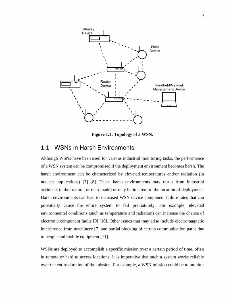
In a WSN, sensor nodes are autonomous devices that are equipped with sensors to measure
certain physical or environment variables, as well as wireless transceivers to communicate
data [5]. In industrial WSNs, devices that collect data are sometimes referred to as field
devices, whereas devices that extend wireless communication range for data forwarding
are called router devices [6]. The collected sensor information is transmitted to pre-
specified collection points, called the sink or gateway, for further analysis by the end users.
A conceptual illustration of a WSN is shown in Figure 1.1.
2
Figure 1.1: Topology of a WSN.
1.1 WSNs in Harsh Environments
Although WSNs have been used for various industrial monitoring tasks, the performance
of a WSN system can be compromised if the deployment environment becomes harsh. The
harsh environment can be characterized by elevated temperatures and/or radiation (in
nuclear applications) [7] [8]. These harsh environments may result from industrial
accidents (either natural or man-made) or may be inherent to the location of deployment.
Harsh environments can lead to increased WSN device component failure rates that can
potentially cause the entire system to fail prematurely. For example, elevated
environmental conditions (such as temperature and radiation) can increase the chance of
electronic component faults [9] [10]. Other issues that may arise include electromagnetic
interference from machinery [7] and partial blocking of certain communication paths due
to people and mobile equipment [11].
WSNs are deployed to accomplish a specific mission over a certain period of time, often
in remote or hard to access locations. It is imperative that such a system works reliably
over the entire duration of the mission. For example, a WSN mission could be to monitor

3
an accident environment or adverse condition for the duration of the event. Alternatively,
the mission could be to monitor a plant process during normal operation between two
consecutive maintenance intervals. It should be noted that in most deployments it may not
be feasible to replace or repair the WSN devices during the mission time. The failure of a
WSN based monitoring system can potentially result in an information blackout that can
negatively affect plant operations, or hinder mitigation activities if the WSN is used to
monitor adverse plant conditions.
It is noted that the existing WSN systems deployed in relatively harsh environment
typically use some kind of environment casing or shielding to protect components, and also
employ some methodology to achieve system level fault-tolerance. System level fault-
tolerance can be achieved by forming redundant communication paths in the network
(through strategic or dense node deployment) to automatically route information when
some nodes fail. In certain applications, however, it might not be feasible to deploy a large
number of devices to attain system level fault-tolerance, for example, in a NPP, as it’s
safety instruments may be sensitive to the EMI from the devices [1]. Instead, device level
fault-tolerance can help enhance the overall WSN system reliability under harsh
environments and can provide fault-tolerance to a system when system level fault-tolerance
may not be practical.
1.2 Redundant WSN Design
As mentioned, harsh environments can increase the rate of component failures in a WSN
device. Therefore, it is feasible to make a device fault-tolerant so that it can operate even
if some of its components may have failed. Fault-tolerant device design is the core
objective of this work. The effect of a fault-tolerant design can be expressed in terms of
reliability, which is defined as the probability that a system will be operational during some
specified mission time. It is noted that reliability is one of the most common ways to
express a system’s fault-tolerance ability [12].
A system’s fault-tolerance can potentially be improved by incorporating redundancy in the
design [13]. Redundancy is the act of replicating critical components in a system, such that

4
some components can remain as backups and assume operation only if the primary
component fails [13].
In a redundant design, a redundancy management system is tasked with detecting and
identifying faulty components, as well as reconfiguring the system when a fault is detected.
Most of the existing redundancy management systems fall into one of the following
approaches: 1) built-in tests (BITs) or 2) voting logic [14].
BITs detect and identify faults by completing a series of in-field tests for each individual
component. These tests could be realized as supplementary hardware or as a software-
based diagnostics algorithm within a component’s existing logic. In WSN devices, both
hardware and software BITs can be implemented to aid in the detection and recovery from
faults [15]. When a fault is detected, the faulty component can be isolated. A backup
component can then assume operation so that a device can continue to function. Figure 1.2
illustrates a redundancy management system using the BIT approach. In Figure 1.2, the
redundancy management system consists of the BITs and the isolation mechanism.
Figure 1.2: BIT approach for redundant components.
The second redundancy management system approach utilizes a voting element to discern
faulty components from correctly working ones. A replicated set of components operate
simultaneously and feed their outputs into a voting unit. Through some predetermined

5
voting criterion (such as majority voting or middle value selection) faulty components can
then be identified [14]. Figure 1.3 illustrates a redundancy management system using the
voting logic approach.
Figure 1.3: Voting logic approach for redundant components.
Each of the two redundancy management approaches comes with their own strengths and
weaknesses. For instance, the BIT approach can be implemented with as little as two
replicated components. It operates on a 1-out-of-n basis, meaning that only 1 replicated
component must be correctly working for the management system to work [14]. The BIT
approach is more suitable for applications that have limited resources. In contrast, the
voting logic approach typically requires a minimum of 3 or more replicated components
and usually operates on a 2-out-of-n basis [14]. Since voting logic requires a higher base
number of replicated components and has a lower bound on the number of operational
components to successfully identify faults, this approach favours applications that are
repairable, i.e., can undergo maintenance during the mission times [16].
In this work, the BIT approach has been used to manage the redundancy of a fault-tolerant
WSN design. The BIT approach has been chosen as it usually requires fewer resources,
which is typically one of the requirements for a WSN system.

6
1.3 Issues with Built-in Tests
Although BITs may be better suited for resource constrained WSNs, some of its own
drawbacks can potentially counteract this approach’s overall reliability improvement. One
of these drawbacks is imperfect fault coverage. Fault coverage is the ability of a system to
correctly detect and identify a faulty component [14]. Imperfect fault coverage results if
certain faults cannot be detected, which can then lead to a complete device failure. For
example, if an undetected fault has occurred in a redundant system, then that fault will not
be mitigated by the redundancy management system. It can be assumed that unmitigated
faults result in a device failure (either directly or indirectly by causing additional faults in
the system) regardless of whether backup components are available.
Another issue with the BIT approach (and redundancy management systems in general) is
the risk of common-cause failures (CCFs) [17]. The elements used in a redundancy
management system to detect, identify and reconfigure faulty components is also
susceptible to failures. Failure of an element of the redundancy management system could
trigger a complete system failure.
To design a fault-tolerant WSN using the BIT approach, both imperfect fault coverage and
CCFs impacts must be effectively addressed.
1.4 Research Objectives, Scope and Methods
1.4.1 Research Objectives
The WSN system, proposed in this work, is assumed to be deployed to perform a
monitoring task during certain critical missions in a harsh environment. Repairing and
replacing system devices during the mission time is not feasible. Furthermore, the proposed
system is particularly suitable for applications where the deployment of a large number of
devices to achieve system level fault-tolerance is not practical.
The objectives of this research are to:
• design a fault-tolerant WSN device that uses the BIT-based redundancy
management system approach.

7
• implement the redundancy management system in prototype WSN devices.
• evaluate the fault-tolerant performance of the redundancy management system.
Specifically, a redundancy management system has been designed that makes use of a
supervisory unit, fault detection hardware and a modular design to address the problem of
imperfect fault coverage and CCFs. This design has been realized in prototype WSN
devices and their performance has been evaluated in an experimental setting.
1.4.2 Research Scope
The proposed design considers fault-tolerant WSN devices with component level
redundancy using the BIT approach. The WSN is assumed to be non-repairable during its
mission time. The design has been realized in a prototype WSN system that is then
evaluated based on assumed and estimated reliability model parameters under simulated
harsh environment conditions. Elevated levels of temperature and radiation have been
considered during the system evaluation. These elevated levels are assumed to not be
severe enough to cause immediate device failures (e.g. components melting). Non-
exhaustive fault injection testing has been used to evaluate the performance of the design.
Note that practical considerations towards WSN implementation, such as energy
provisioning, power consumption and communication protocols, are only partially
considered as they are beyond the scope of this work.
1.4.3 Methods
This work is divided into four steps: first, redundancy management approaches have been
investigated to identify potential techniques that can be used to improve fault coverage and
to reduce the impact of CCFs. Next, a redundancy management system is designed. In the
third step, this design is implemented in a WSN system. In the final step, the performance
of the implemented design has been evaluated through reliability analysis, fault injection
testing and an industrial test deployment.

8
1.5 Organization
The remainder of this work is organized as follows. Relevant literature on fault-tolerant
systems, the impact of harsh environments on electronic components and redundancy
management systems have been reviewed in Chapter 2. Modelling and analysis of
imperfect fault coverage and CCFs have been discussed in Chapter 3. In Chapter 4, the
redundancy management system design is presented. Chapter 5 has described the
implementation of a prototype WSN system, and Chapter 6 has presented the evaluation
results. Finally, the work has been concluded with a summary and the contributions in
Chapter 7.

9
Chapter 2
2 Background & Literature Review
In this chapter, some background information on fault-tolerant systems and the impact of
harsh environments on electronic components are discussed. Different approaches for a
redundancy management system using BITs as well as existing WSNs for harsh
environments are also reviewed.
2.1 Fault-Tolerant Systems
Fault-tolerance is a term used to describe the ability for a system to operate correctly,
despite the presence of errors or faults [13]. Three core principles govern the various
approaches for implementing fault-tolerance that can improve system reliability. A variety
of methods exist to model and analyze a system’s reliability. These methods and models,
along with some literature on existing redundancy management systems, are discussed
next.
2.1.1 Principles and Evaluation Metrics
Fault-tolerance is built upon three core design principles: redundancy, diversity and
independence [13]. Each of these design principles can be used in conjunction with each
other to enhance a system’s reliability.
As mentioned previously, redundancy is the act of replicating critical components in a
system, such that some components can remain as backups and assume operation only if
the primary component fails. Redundancy is usually implemented for more critical
components that either have a higher chance of failure or are essential for correct system
operation. Redundancy can be active or passive [13]. Active redundancy describes when
the redundant components operate concurrently, enabling immediate substitution of a
faulty component. In passive redundancy, backup components remain in a standby state
until needed.
Diversity in a design holds many similarities with redundancy as it relates to redundant
components. A diverse component is one that is functionality equivalent such that it can

10
assume operation if the primary component fails, however its functionality is derived from
different underlying mechanisms or construction. For example, powering an electronic
device with a primary AC power supply and backup DC power supply would be considered
as diverse. The advantage with using diverse backups occurs when failure modes are
different between the components. Continuing with the power supply example, if an AC
supply requires a power-grid connection, whereas a DC supply is powered through an
external battery pack, then these two components have different failure modes. If the AC
supply fails due to the loss of the grid connection, the DC supply would not be inherently
impacted by this failure mode. To contrast this scenario, if the two power supplies depend
upon a common set of voltage regulators that then becomes damaged, both power supplies
can be impacted and fail simultaneously (note that failure here is defined as the inability to
perform the intended operation). This type of failure scenario is often referred to as a CCF
or a single point of failure.
Lastly, independence in design refers to the exclusion or separation of components such
that a failure in one component does not impact the operation of the other components. A
transformer is a common example of independence in design since certain types of faults
are not directly translated between the primary and secondary windings.
As mentioned, reliability can be used to express the ability of a system to tolerate faults
[12]. For a system with a constant failure rate, 𝜆, the reliability function is described as
𝑝(𝑡) = 𝑒−𝜆𝑡, (2.1)
with 𝑡 being the time and 𝑝(𝑡) being the reliability at a given time. The higher the
reliability, the greater the chance that a system will be operational at time 𝑡. Another metric
often associated with a system’s reliability is mean time to failure (MTTF) [18] which is
the expected time to failure. For a system with a constant failure rate, MTTF is defined as
𝑀𝑇𝑇𝐹 = 1
𝜆. (2.2)
When comparing systems of varying complexity, a normalized MTTF timescale can be
used, which is defined as

11
𝑛𝑜𝑟𝑚𝑎𝑙𝑖𝑧𝑒𝑑 𝑀𝑇𝑇𝐹 =𝑡
𝑀𝑇𝑇𝐹. (2.3)
A normalized timescale can be used to compare reliability improvements in a design while
abstracting away details that relate a system’s specific failure rate [17].
To evaluate a system’s reliability, a model must first be developed that sufficiently
represents the failure characteristics of a system. One of the simplest methods of modelling
reliability is with reliability block diagrams (RBDs) [18]. By identifying the various failure
modes of a system’s components, component failure rates and the system’s architecture, a
model that represents the relationship between component failures and a complete system
failure can be developed. For example, Figure 2.1 illustrates a RBD for a WSN gateway
device. In this diagram, there are five key components: a radio unit, a processor unit, a
memory unit, a power management unit, and a network interface unit. The first four
components have no replication and are therefore represented as a single block. The
network interface unit, however, has n replicated units and is therefore represented as n
blocks in parallel.
Figure 2.1: Example of a reliability block diagram for a WSN gateway device.
Another common method to evaluate a system’s reliability is through the use of a fault tree
[18]. A fault tree is similar to RBDs, but it is instead a more visual approach to represent a
system based on its failure modes. To illustrate, a fault tree is shown in Figure 2.2 for a
three-device WSN along with the WSN topology: a field device connected to a gateway
device through a router. In Figure 2.2, the system failure condition incorporates the WSN’s

12
topology, as any device failure would result in a loss of information from the field device.
Each device failure is composed of multiple initiating conditions as represented by the
circles. An OR gate is used to relate the different failure conditions together, indicating that
any failure condition results in a complete device failure. An AND gate is used to indicate
that all initiating conditions must occur for that gate to be activated.
Figure 2.2: Fault tree for three WSN devices.
2.1.2 Impact of Harsh Environments on Electronic Components
As already stated in Chapter 1, harsh environments can negatively impact the reliability of
a system by elevating the failure rates of components. Special consideration must be taken
to accurately reflect an individual component’s failure rate when developing a reliability
model, since grossly inaccurate failure rates can render a model useless.
Most component manufacturers provide failure rate data for their various passive and
active electronic components under an expected operating environment. Since industrial
applications can have harsh and variable environmental conditions, this standard failure
rate data alone may not be enough, and the failure rates may need to be estimated. For this
13
estimation, the manufacturer provided failure rates can be scaled by various degradation
and acceleration factors under these alternate environmental conditions [19].
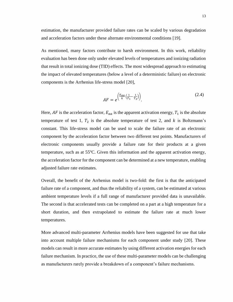
As mentioned, many factors contribute to harsh environment. In this work, reliability
evaluation has been done only under elevated levels of temperatures and ionizing radiation
that result in total ionizing dose (TID) effects. The most widespread approach to estimating
the impact of elevated temperatures (below a level of a deterministic failure) on electronic
components is the Arrhenius life-stress model [20],
𝐴𝐹 = 𝑒(
𝐸𝑎𝑎𝑘
(1
𝑇1−
1
𝑇2))
.
(2.4)
Here, 𝐴𝐹 is the acceleration factor, 𝐸𝑎𝑎 is the apparent activation energy, 𝑇1 is the absolute
temperature of test 1, 𝑇2 is the absolute temperature of test 2, and 𝑘 is Boltzmann’s
constant. This life-stress model can be used to scale the failure rate of an electronic
component by the acceleration factor between two different test points. Manufacturers of
electronic components usually provide a failure rate for their products at a given
temperature, such as at 55oC. Given this information and the apparent activation energy,
the acceleration factor for the component can be determined at a new temperature, enabling
adjusted failure rate estimates.
Overall, the benefit of the Arrhenius model is two-fold: the first is that the anticipated
failure rate of a component, and thus the reliability of a system, can be estimated at various
ambient temperature levels if a full range of manufacturer provided data is unavailable.
The second is that accelerated tests can be completed on a part at a high temperature for a
short duration, and then extrapolated to estimate the failure rate at much lower
temperatures.
More advanced multi-parameter Arrhenius models have been suggested for use that take
into account multiple failure mechanisms for each component under study [20]. These
models can result in more accurate estimates by using different activation energies for each
failure mechanism. In practice, the use of these multi-parameter models can be challenging
as manufacturers rarely provide a breakdown of a component’s failure mechanisms.

14
MIL-HBDK-217 [21] is a military handbook produced to aid in determining accurate
failure rate data for electronic components. Based on experimental and field data, this
handbook provides scaling factors (including temperature induced acceleration factors)
that can be used to adjust a component’s failure rate to a wide variety of environmental
conditions. MIL-HBDK-217 also provides scaling factor adjustments for military
environments (such as on naval ships or when airborne). Based on the scaling method
suggest in this handbook, failure rates are scaled as follows,
𝜆′ = 𝜆𝜃, (2.5)
where 𝜃 is the scaling term and 𝜆′ is the new component failure rate. Equations provided
in MIL-HBDK-217 can be used to solve for 𝜃 based on the environmental conditions and
the type of electronic component. Note that if the failure rate for a non-military
environment is to be estimated using MIL-HBDK-217, the only scaling term would come
from the temperature acceleration factor, resulting in
𝜆′ = 𝜆𝐴𝐹. (2.6)
Neither MIL-HBDK-217 nor the more modern JEP122 account for the impact of ionizing
radiation in the failure rates of electronic components. Instead, a second scaling term called
the radiation degradation factor, Δ𝑘, is required to estimate the negative impact of this harsh
environmental condition [22]. With the use of Δ𝑘, the failure probability of an electronic
component can be scaled to estimate the new failure probability after receiving a specified
TID,
𝑝(𝑡)′ = (1 − Δ𝑘)𝑒−𝜆𝑡. (2.7)
Similar to 𝐸𝑎𝑎, the radiation degradation factor is experimentally determined. The work in
[23] along with the NASA Goddard Space Flight Center radiation test database [24] can
be used to estimate this degradation factor, thus enabling reliability estimates under varying
levels of ionizing radiation.
Both scaling techniques can be combined as follows to provide a more accurate reliability
approximation under an environment with higher levels of temperature and radiation,

15
𝑝(𝑡)′ = (1 − Δ𝑘)𝑒−𝜆′𝑡, (2.8)
with 𝑝(𝑡)′ being the approximated component reliability.
2.1.3 Redundancy Management Systems Using the BIT Approach
The primary issue with the BIT approach is imperfect fault coverage [14]. Coverage
describes the probability that a fault will be correctly identified through some protection
scheme. Perfect fault coverage results in most voting-based systems where a comparison
between multiple outputs can detect the occurrence of a fault. On the other hand, BITs have
imperfect fault coverage due to the difficulties that arise when detecting a fault through
some sort of self-test. Even with high levels of coverage (nearing 99%), a significant
negative impact on a system’s reliability occurs [14]. Therefore, circumventing this
imperfect coverage issue is the primary challenge faced with BITs.
BIT coverage can be improved by enhancing fault detection capabilities. A significant
portion of the literature has focused on fault detection and identification by using a variety
of techniques that fall under model-based, signal-based, knowledge-based, and hybrid
approaches [25] [26]. Although these approaches are powerful in the correct setting, their
use is relatively limited for detecting embedded systems faults in a WSN device.
A BIT-based system structure that uses a comparator has been proposed in [27]. In their
work, comparison logic (similar to voting logic) and BITs are used simultaneously in a
dual-redundant system. Figure 2.3 illustrates this arrangement. The advantage of the
comparison logic is that a fail-safe mechanism is introduced that can halt a system’s
operations under certain output conditions. This fail-safe mechanism, however, does not
improve a system’s fault coverage, since the system ceases to operate when this mechanism
is activated.

16
Figure 2.3: Redundancy management with BITs and comparison logic.
The other major challenge for the BIT approach is the introduction of additional CCF
mechanisms. If, for example, a switch that is used to select a redundant system’s output
becomes damaged, then this faulty switch could result in a complete system failure. This
added risk introduced by the redundancy management system in some cases can reduce a
system’s reliability rather than improve it [17]. To better understand the relationship
between a potential reliability improvement from a redundant design, a redundancy-
relevance boundary has been proposed in [17]. Their work emphasizes the importance of
considering how CCFs can impact a redundant design and has been discussed further in
Chapter 3.
2.2 WSNs for Harsh Environments
There are a variety of target applications for WSN devices in harsh environments, from
industrial use to disaster relief scenarios. In this section, WSN device-level architectures
and existing techniques employed in WSNs for harsh environment applications are
reviewed.
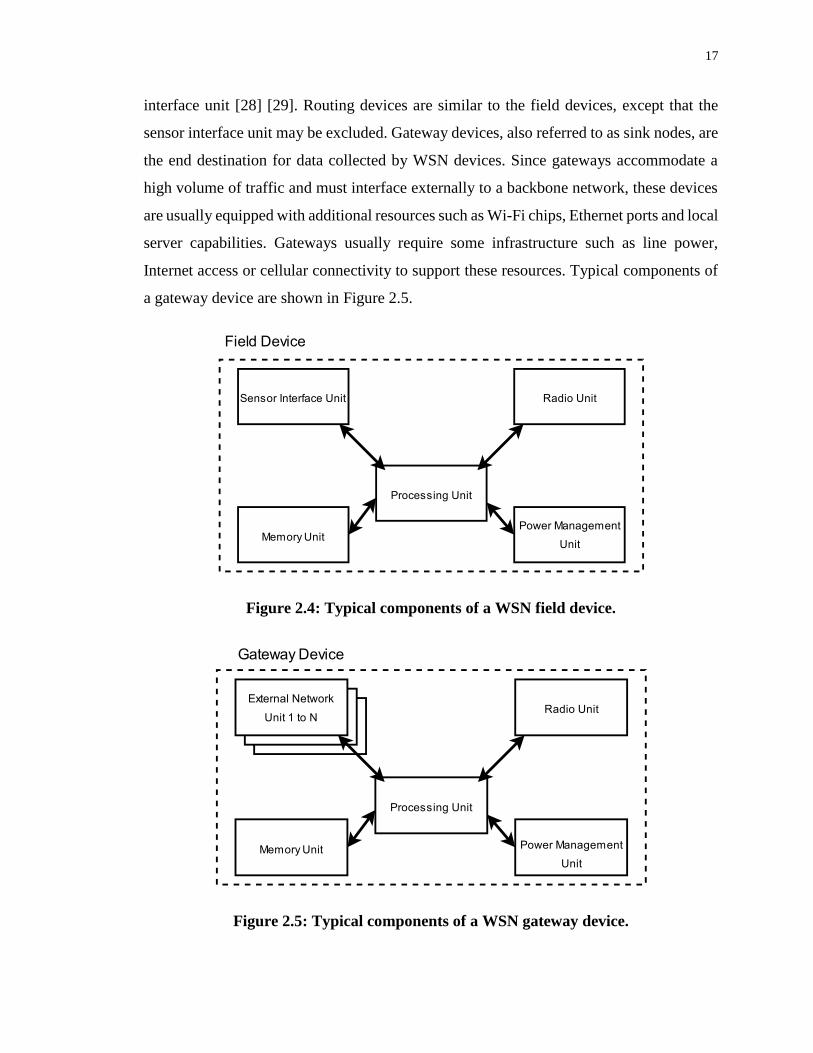
2.2.1 Device-Level Architecture
WSN devices consist of several key components, as shown in Figure 2.4. Field devices
consist of a radio unit, processor unit, memory unit, power management unit, and a sensor
17
interface unit [28] [29]. Routing devices are similar to the field devices, except that the
sensor interface unit may be excluded. Gateway devices, also referred to as sink nodes, are
the end destination for data collected by WSN devices. Since gateways accommodate a
high volume of traffic and must interface externally to a backbone network, these devices
are usually equipped with additional resources such as Wi-Fi chips, Ethernet ports and local
server capabilities. Gateways usually require some infrastructure such as line power,
Internet access or cellular connectivity to support these resources. Typical components of
a gateway device are shown in Figure 2.5.
Figure 2.4: Typical components of a WSN field device.
Figure 2.5: Typical components of a WSN gateway device.

18
2.2.2 Existing Monitoring Systems in Harsh Environments
Some work has been done to develop different WSN systems that are more suited for use
in disaster response scenarios, as summarized in [30]. Seven different system topologies
have been identified that make use of multiple wireless communication technologies such
as satellite, wide area networks and personal area networks. The use of multiple wireless
technologies and wireless channels within a single system can improve information
availability in a network [22]. Some other work has proposed the use of multi-radio WSN
devices [31] to allow for the integration of multiple WSN technologies on one board (such
as Bluetooth and Zigbee).
There are some custom-made, robust wireless monitoring systems developed primarily for
military applications [32], [33]. These systems include casings or shielding to provide
protection against adverse environmental conditions. The primary objective for these
monitoring systems is reliable, long-range communication. Therefore, these systems
transmit information directly to their end devices by using satellite, cellular or other long-
range technologies.
Other wireless monitoring solutions rely upon the use of advanced materials and simple
circuits that are less susceptible to failures in harsh environments. In [34], a specialized
wireless telemetry system has been developed that can withstand temperatures greater than
350oC. Similarly, a wireless pressure sensing solution for high temperatures has been
developed in [35] that relies upon a simple circuit design and FM technology.
A recent work has proposed a wireless monitoring system for NPPs under severe accident
conditions [23]. Their objective has been to design a radiation-tolerant system using
commercial off-the-shelf components. The system has used radiation shielding and a
redundant design that is based on voting logic.
2.3 Limitations of Existing Work
In general, existing WSN systems for harsh environments use a combination of protective
casing for the devices and system level fault-tolerance (such as ensuring redundant
communication paths in the network). Protective casings create a physical barrier between

19
devices and the harsh environment, reducing the environment’s negative impact on a
device’s reliability. However, their effectiveness can be limited. For example, elevated
ambient temperatures and certain types of ionizing radiation can penetrate through
protective casing. Although, in general, protective casing can reduce the impact of harsh
environment to a certain degree, the penetrating effect may still result in conditions that are
higher than the typical operating environment for a WSN device. Applying additional
protection to a system to mitigate this effect may not be practical. For example, radiation
shielding can be used to reduce the TID received by a WSN device, but radiation shielding
can be an expensive and heavy solution.
The topologies summarized in [22] can enhance system level fault-tolerance by
incorporating multiple wireless communication technologies into a WSN. For these
topologies to be effective, the deployment of their nodes must be restricted to either a
strategic or dense deployment. This restricted deployment may not be achievable in certain
applications, limiting their applicability.
Many of the wireless monitoring systems developed for military applications use long-
range communication technologies that can have difficulty in indoor, industrial
environments. For example, wireless signals may not be able to penetrate through the thick
concrete walls of a containment building in a NPP.
The specialized wireless monitoring systems with advanced materials for use in high
temperature applications rely upon simple RF circuit technology for point-to-point
communication. These systems may not be suitable for use in harsh environments if the
sensor information cannot be transmitted directly to a base station. For example, within the
containment building in a NPP, mesh networking might be the only option to relay
environmental data wirelessly to a sink device. These types of systems are also not
developed for environments with high levels of ionizing radiation.
In [23], device level fault-tolerance has been achieved with a redundant design based on
the voting logic approach. Their design has focused on radiation-tolerant design in the
circuit and system level.

20
Overall, protective casings and system level fault-tolerance techniques can have a limited
effectiveness in certain applications and deployments. Device level fault-tolerance by
incorporating redundancy in a design can be used to improve WSN system reliability.
Device level fault-tolerance can also be used in addition to protective casing and system
level fault-tolerance to further improve WSN reliability for certain critical applications,
such as monitoring an industrial plant during an accident condition. For device level fault-
tolerance from a redundant design to be an effective solution, the issues of imperfect fault
coverage and CCFs have to be addressed. The remainder of this work details the
development of a BIT-based redundancy management system that address these two issues.

21
Chapter 3
3 Modelling Imperfect Fault Coverage
The design of a redundancy management system for WSN devices begins with the
development of an appropriate reliability model. In this chapter, imperfect fault coverage
is first modelled under ideal conditions, in which no CCFs are introduced. An approach to
improve coverage through the use of a supervisory unit is then presented. Afterwards, a
more advanced reliability model is developed that includes the impact of both imperfect
fault coverage and CCFs. Finally, a modularized architecture that could further diminish
some of the negative aspects of CCFs is discussed.
3.1 Modelling Imperfect Fault Coverage Without CCFs
In the development of a model for a redundant system, the following assumptions are:
• The failure rate 𝜆 is constant in a given operating environment.
• Redundant components are in an active state.
• Redundant components are identical, such that 𝜆1 = 𝜆2 = 𝜆𝑛 = 𝜆.
• Failures are independent and permanent among all components.
Note that dependant component failures are modelled separately as CCFs in Section 3.2.
As well, component failure rates could be time-dependant if environmental conditions
(such as temperature) change. Therefore, the impact of a non-constant failure rates on the
developed models will be discussed throughout this chapter when relevant.
Under the previous assumptions, the reliability for a device consisting of a single
component can be derived from an exponential distribution as detailed in [14],
𝑝(𝑡) = 𝑒−𝜆𝑡 (3.1)

22
If a single device requires two identical components to be functioning at the same time, it
is not redundant. The corresponding reliability model would simply be the product of
reliability of the two components,
𝑅(𝑡) = 𝑒−𝜆𝑡𝑒−𝜆𝑡 = 𝑒−2𝜆𝑡. (3.2)
Instead, if a single device consists of two identical components, and only one component
needed to be operational for the device to work, then the device would be described as
dual-redundant. The reliability model for such a device relates to the parallel product of the
reliability of each component [14],
𝑅(𝑡) = 1 − (1 − 𝑒−𝜆𝑡)(1 − 𝑒−𝜆𝑡) = 1 − (1 − 𝑒−𝜆𝑡)2. (3.3)
In general, the reliability for an 𝑛-redundant device is
𝑅(𝑛, t) = 1 − (1 − 𝑒−𝜆𝑡)𝑛
. (3.4)
Equation (3.4) assumes perfect fault coverage (or that a fault does not need to be detected
for the system to continue to operate). As noted in Section 2.1.3, this perfect level of
coverage is usually not achievable in a BIT based approach.
The BIT approach operates on a 1-out-of- 𝑛 basis [14], meaning that the system can
continue to work if at least 1 replicated component is still functional. The reliability for
such a system is given as
𝑅(𝑛, 𝑝(𝑡)) = ∑ (𝑛
1) 𝑝𝑖(1 − 𝑝)𝑛−𝑖𝑛
𝑖=1 (3.5)
where 𝑅 is the device reliability, and 𝑝 is the component reliability. In contrast, the general
model for a voting logic system operating on a 2-out-of- 𝑛 basis is
𝑅(𝑛, 𝑝(𝑡)) = ∑ (𝑛
1) 𝑝𝑖(1 − 𝑝)𝑛−𝑖𝑛
𝑖=2 . (3.6)
One method to express imperfect fault coverage is to separate a component’s failure rate
into covered and uncovered faults as such:

23
𝜆 = 𝜆𝑐 + 𝜆𝑢𝑐, (3.7)
where 𝜆𝑐 is the covered fault failure rate and 𝜆𝑢𝑐 is the uncovered fault failure rate [14].
The entire system’s failure rate, 𝜆, can be split into the faults that can be detected, 𝜆𝑐, and
the faults that cannot be detected, 𝜆𝑢𝑐. Coincidentally, in this work, a covered fault can be
detected whereas an uncovered fault cannot be detected. An alternate approach to express
fault coverage is through a component’s coverage ratio, 𝑐 [14]. Following from Equation
(3.7), the relationship between the covered and uncovered failure rate is
𝜆𝑐 = 𝑐𝜆, (3.8)
and
𝜆𝑢𝑐 = (1 − 𝑐)𝜆. (3.9)
Before developing the reliability model for a system with imperfect fault coverage, first
the reliability impact of 𝜆𝑐 and 𝜆𝑢𝑐 needs to be understood. If, for example, a detectable
fault (𝜆𝑐) has occurred in one component of a dual-redundant device, that device could
substitute the correctly operating component for the faulty component. If, instead, an
undetectable fault (𝜆𝑢𝑐) has occurred in the same device, that fault would go unmitigated
in the system and the device would enter into a failed state.
Fault coverage can be incorporated into the reliability model developed in Equation (3.4),
as detailed in [14], yielding
𝑅(𝑛, 𝑝(𝑡), 𝒄) = ∑ 𝒄𝑻(𝑖, 𝒄) (𝑛
1) 𝑝𝑖(1 − 𝑝)𝑛−𝑖𝑛
𝑖=1 , (3.10)
where 𝒄𝑻(𝑖, 𝒄) is the set of products of the 𝑘-subset of the coverage ratio vector, 𝒄, with
exactly 𝑛 − 𝑖 elements. The coverage ratio vector for an 𝑛-redundant system is 𝒄 =
{𝑐1, … , 𝑐𝑛}. For a triple-redundant system (𝑛 = 3), the 𝒄𝑻 set would be
𝒄𝑻(1, 𝒄) = {𝑐1𝑐2, 𝑐1𝑐3, 𝑐2𝑐3}
𝒄𝑻(2, 𝒄) = {𝑐1, 𝑐2, 𝑐3}
𝒄𝑻(3, 𝒄) = {1} .

24
Each component has been assumed to be identical,
𝑐1 = 𝑐2 = 𝑐𝑛 = 𝑐. (3.11)
From Equation (3.10) it can be seen that the uncovered faults negatively impact the
reliability of the system, with a smaller fault coverage leading to a reduction in reliability.
If 𝑐 = 0 in a dual-redundant system, the model reverts back to Equation (3.2) where a
failure in either component results in a device failure. If 𝑐 = 1, the system reverts to
Equation (3.3), a dual-redundant system with perfect coverage.
To illustrate this, Figure 3.1 depicts the reliability curve for a dual-redundant system under
imperfect fault coverage conditions. The y-axis represents the reliability, 𝑅, for a dual-
redundant device, and the x-axis represents the time 𝑡 normalized by the MTTF for a single
component system. Perfect coverage is when 𝑐 = 1, and imperfect coverage is when 0 <
𝑐 < 1. A clear observation from Figure 3.1 is that as the coverage ratio decreases, the
reliability diminishes. Conversely, improving the coverage ratio would improve the
system’s reliability.
Figure 3.1: System reliability under imperfect fault coverage.
Normalized Time t
Reliability R
Single component
Dual-redundant
perfect coverage
Dual-redundant
imperfect coverage
Increased reliability
as c increases
Reduced reliability
as c decreases

25
The results in Figure 3.1 can be explored further to better understand the significance of
imperfect fault coverage on a system. A question that can be raised is whether the use of
redundancy in a system can be harmful rather than beneficial? To answer this question, a
redundancy-relevance boundary for a BIT-based system with a varying level of redundancy
(LR) and imperfect fault coverage has been developed. This boundary is shown in Figure
3.2. Here, a redundancy level of 0 represents a system with no redundancy, whereas a
redundancy level of 1 represents a dual-redundant system.
Figure 3.2: Redundancy-relevance boundary for a BIT-based system.
This boundary shows the minimum coverage level required for a redundant system to
improve the MTTF relative to a non-redundant system. For a dual-redundant system (with
LR=1), a coverage ratio greater than 0.5 is required. To contrast, a triple-redundant system
requires the coverage ratio to be greater than 0.605. Ensuring that the coverage ratio is
larger than this boundary condition is imperative to successfully improve the reliability in
a redundant system.
Coverage
Level of Redundancy LR
In this region,
MTTF is improved
In this region, imperfect
fault coverage results in an
overall MTTF reduction
26
Recall the discussion of the comparator block presented in Section 2.1.3. It has been
identified that the weakness of this supplementary detection system is its inability to
improve fault coverage. What if instead this comparator block served a dual-purpose,
capable of detecting a malfunction and providing additional means to identify the fault? If
this supplementary block is more capable (perhaps able to provide additional information
to the existing BITs or providing new identification mechanisms), it could improve a
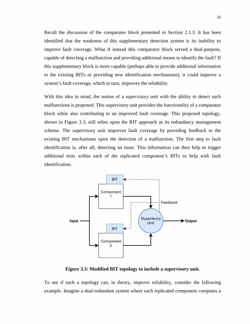
system’s fault coverage, which in turn, improves the reliability.
With this idea in mind, the notion of a supervisory unit with the ability to detect such
malfunctions is proposed. This supervisory unit provides the functionality of a comparator
block while also contributing to an improved fault coverage. This proposed topology,
shown in Figure 3.3, still relies upon the BIT approach as its redundancy management
scheme. The supervisory unit improves fault coverage by providing feedback to the
existing BIT mechanisms upon the detection of a malfunction. The first step to fault
identification is, after all, detecting an issue. This information can then help to trigger
additional tests within each of the replicated component’s BITs to help with fault
identification.
Figure 3.3: Modified BIT topology to include a supervisory unit.
To see if such a topology can, in theory, improve reliability, consider the following
example. Imagine a dual-redundant system where each replicated component computes a

27
number based on its input that then sends this value as a signal through a communication
channel. Before this output value is sent, a BIT re-checks that the computed value is correct.
Unknown to the BIT, however, is that noise might occasionally interfere with only one of
the output signals being sent from the two components, which coincidentally changes the
output value. If an intermediate element (the proposed supervisory unit) has received this
signal, a mismatch between the two components could be detected when noise interferes
with the signal. When this situation occurs, this fault information is fed back to each
component’s BIT. By feeding back the corresponding output signals, a BIT could then
conclude that the signal received is not the signal intended to be sent. In turn, the
component with the noisy communication line could be identified and isolated, allowing
the alternate component to resume operation.
Quantitively, a supervisory unit can be incorporated into a reliability model to study its
impact. A new variable denotes the added fault coverage provided by the supervisory unit,
called the supervisory coverage ratio, 𝑐𝑠. This supervisory coverage ratio provides an
additive effect with the existing system’s original coverage, 𝑐. For example, if a system
has a coverage ratio of 𝑐 = 0.5 and the supervisory unit can detect and identify an
additional 10% of faults, then 𝑐𝑠 = 0.1. The system’s new coverage ratio, 𝑐′, would then
be
𝑐′ = 𝑐 + 𝑐𝑠. (3.12)
A new reliability model can be produced that includes this additive coverage effect,
𝑅(𝑛, 𝑝(𝑡), 𝒄′) = ∑ 𝒄𝑻(𝑖, 𝒄′) (𝑛
1) 𝑝𝑖(1 − 𝑝)𝑛−𝑖𝑛
𝑖=1 . (3.13)
This model, however, is not yet complete since the supervisory unit (like all components)
can fail. As well, the supervisory unit can also provide false information. It would therefore
have a corresponding failure rate, 𝜆𝑠, and a false positive rate, 𝜆𝑓, along with its own
MTTF, denoted by MTTFs. The replicated components have their MTTF denoted by
MTTFc. If the supervisory unit is assumed to be fail-safe (it cannot result in a CCF and any
false positives can be corrected for, such that 𝜆𝑓 = 𝜆𝑠), its failure cannot result in a system
failure, but the added coverage improvement would be lost.

28
How can this loss of coverage condition that arises when the supervisory unit suffers from
a failure be effectively incorporate into a reliability model? In a sense, such behaviour
dynamically alters a reliability model that can complicate matters.
A simple approach can be taken to estimate its effects. Consider the following three
situations:
1. The supervisory unit cannot fail (or is highly unlikely to fail).
2. The supervisory unit has a similar failure rate to the replicated components.
3. The supervisory unit will fail significantly sooner than the replicated components.
In the first situation, it would be expected that the full fault coverage benefit of the system
can be obtained. That is, the reliability model would be Equation (3.13).
In the second situation, at some point the supervisory unit will fail. It would therefore make
sense that initially a reliability improvement is achieved close to the maximum achievable
improvement from Equation (3.13). As time progresses, however, the likelihood that the
supervisory unit has failed increases. The reliability should therefore rest somewhere below
the upper bound. As time extends out further, the system would perform as if no
supervisory unit has been added and approach the lower bound in Equation (3.10).
In the third situation, it would be expected that the supervisory unit provides a marginal
improvement since its failure should occur rather quickly. The system’s reliability should
be expected to quickly approach the lower bound in Equation (3.10).
From these three scenarios, it can be concluded that the proposed system’s reliability
should be bounded at all times by Equation (3.10) and Equation (3.13). Further, the
reliability improvement depends upon the supervisory unit’s failure rate, 𝜆𝑠 and the
replicated component’s, 𝜆. A decay in the reliability improvement is expected as time
progresses based on some ratio of these two failure rates.
A reliability model has been developed that satisfies the previous conditions:
𝑅(𝑛, 𝑝(𝑡), 𝒄′(𝛼)) = ∑ 𝒄𝑻(𝑖, 𝒄′)) (𝑛
1) 𝑝𝑖(1 − 𝑝)𝑛−𝑖𝑛
𝑖=1 , (3.14)

29
where 𝛼 is the coverage decay function
𝛼 = 𝑒
− 𝑀𝑇𝑇𝐹𝑐𝑀𝑇𝑇𝐹𝑠 = 𝑒− 𝛾
(3.15)
and 𝑐′ is
𝑐′(𝛼) = 𝑐 + 𝛼 𝑐𝑠. (3.16)
Note that 𝛾 is the ratio of the two MTTFs. The effect of this decay function on the reliability
model is shown in Figure 3.4. Note that the model’s reliability satisfies the previously
described conditions, as it is effectively bounded between Equation (3.10) and Equation
(3.13).
Figure 3.4: Bounding effect of the coverage decay function.
Note here that the model developed in Equation (3.14) is merely an estimate to better
understand the impact of a fail-safe supervisory unit that is subject to failures. As such, a
Normalize time t
Reliability R
pper Bound
Lower Bound
MTTFs MTTF
c
MTTFs MTTF
c
MTTFs MTTF
c

30
rigours proof is not provided or needed to gather insight towards the value of the
supervisory unit in a redundant design. Ultimately, for this model to be deemed correct
(either as conservative or optimistic) additional testing is required. Nevertheless, insight
towards the desirable traits of the postulated supervisory unit can be extracted.
The first insight from Figure 3.4 is that if the supervisory unit is fail-safe, then no harm can
come to the system’s overall reliability. Second is that the failure rate of the supervisory
unit influences its reliability improvement. Ideally, a failure rate much smaller than the
component’s rate would yield the greatest improvement. If these two failure rates are
similar to each other, a smaller yet significant reliability improvement is gained.
Note that in scenarios with non-constant failure rates (such as when an environment
changes), it is important to ensure that the supervisory unit’s failure rate is equal to or lower
than the component’s failure rate. To determine whether this condition is met, failure rates
can be calculated under a variety of expected environmental conditions using the scaling
factors presented in Section 2.1.2.
In summary, an alternate BIT topology has been proposed that uses a supervisory unit to
improve fault coverage, and ergo, reliability. This reliability improvement hinges on the
failure rate of the added unit. Both the BITs and the supervisory unit can introduce
additional failure mechanisms in a system that can negatively impact the reliability. These
considerations are discussed next.
3.2 Modelling Imperfect Fault Coverage with CCFs
The previous model has not considered the impact of any additional CCFs. A more realistic
reliability model needs to be developed that includes this fact. The objective of such a
model is to identify the boundary condition in which a system’s reliability is improved
given the model parameters.
One conservative approach for modelling CCFs in a redundant design is the 𝛽-factor model
[36]. The 𝛽-factor is a single parameter approach to modelling the probability of an event
occurring, and is defined as the ratio of the CCF rate to the total failure rate of the
components,

31
𝛽 = 𝜆𝐶𝐹𝐹
𝜆+ 𝜆𝐶𝐶𝐹 . (3.17)
This 𝛽-factor can be included in the previously derived reliability model for a redundant
system,
𝑅(𝑛, 𝑝(𝑡), 𝛽, 𝜆) = ( ∑ (
𝑛
1) 𝑝𝑖(1 − 𝑝)𝑛−𝑖𝑛
𝑖=1 ) 𝑒−
𝛽
1−𝛽𝜆𝑡
. (3.18)
Equation (3.18) represents the reliability model for an idealized redundant system. For a
system constructed with the BIT approach, the respective reliability model is
𝑅(𝑛, 𝑝(𝑡), 𝒄, 𝛽, 𝜆) = (∑ 𝒄𝑻(𝑖, 𝒄) (
𝑛
1) 𝑝𝑖(1 − 𝑝)𝑛−𝑖𝑛
𝑖=1 ) 𝑒−
𝛽
1−𝛽𝜆𝑡
, (3.19)
whereas the voting logic approach would have
𝑅(𝑛, 𝑝(𝑡), 𝛽, 𝜆) = ( ∑ (
𝑛
1) 𝑝𝑖(1 − 𝑝)𝑛−𝑖𝑛
𝑖=2 ) 𝑒−
𝛽
1−𝛽𝜆𝑡
(3.20)
as its reliability model.
A similar redundancy-relevance boundary to that in Figure 3.2 can be developed to
compare the effective reliability improvement of these two approaches. This boundary is
shown in Figure 3.5 under a varying level of redundancy.

32
Figure 3.5: Redundancy-relevance boundary for both redundancy approaches.
As shown in Figure 3.5, there is a maximum value of the 𝛽-factor for each level of
redundancy after which the reliability, in terms of the MTTF, would decrease rather than
improve. For a BIT-based triple-redundant system, this value is 0.379. In contrast, for a
triple-redundant voting logic-based approach, even with 𝛽 = 0 (no CCFs), a MTTF-based
reliability improvement cannot be achieved. This result illustrates as to why voting logic
might not be as well suited for certain non-repairable monitoring applications using WSN
systems. For example, if a voting logic system is non-repairable and is intended to operate
until failure, it is expected that this system would fail sooner than a non-redundant system.
The cause of this earlier failure stems from the increased number of components in a
redundant system that increases the occurrence of component failures within the same time
interval. Coincidentally, redundant components decrease the mean time between failure
(MTBF) within a system. Using a triple-redundant system operating on a 2-out-of- 𝑛 basis

33
as an example, this decreased MTBF means that two components are expected to fail within
the normalized MTTF interval, reducing this system’s MTTF.
A reliability model can now be produced that incorporates both imperfect fault coverage
and CCFs for BIT-based systems as follows,
𝑅(𝑛, 𝑝(𝑡), 𝒄, 𝛽, 𝜆) = (∑ 𝒄𝑻(𝑖, 𝑐) (
𝑛
1) 𝑝𝑖(1 − 𝑝)𝑛−𝑖𝑛
𝑖=1 ) 𝑒−
𝛽
1−𝛽𝜆𝑡
. (3.21)
Based on this model, a more advanced redundancy-relevance boundary can be developed.
This new boundary is shown in Figure 3.6. Note that the reliability reduction that results
from imperfect fault coverage and CCFs is additive; a reduction in fault coverage
necessitates an improvement in the 𝛽-factor, and vice versa.
Figure 3.6: Advanced redundancy-relevance boundary considering imperfect fault
coverage and CCFs.

34
This boundary can be used as a design tool, enabling quick reliability analysis of a
redundant system. Given the estimates for a system’s fault coverage, its 𝛽-factor, and the
level of redundancy, a designer can determine whether a reliability improvement is
achieved.
The redundancy-relevance boundary in its current form does not indicate the magnitude of
the reliability improvement. Once a design is deemed to improve reliability, it is desirable
to determine the level of improvement.
In this regard, a reliability-improvement plane for each level of redundancy can be
produced from Equation (3.21). By normalizing the factor of improvement against a non-
redundant system’s MTTF, the relative improvement can be determined. Figure 3.7 shows
this relative improvement under different levels of redundancy.
These individual planes can be used to determine the anticipated reliability improvement
given the appropriate model parameters. For example, a triple-redundant system’s level of
redundancy is two. By examining the top right plane in Figure 3.7, it can be seen that the
maximum MTTF improvement is 1.83 times greater than that of a non-redundant system.
This improvement is only attained when the coverage is equal to one and the 𝛽-factor is
equal to zero.
The proposed supervisory unit now can be integrated with the reliability model produced
in Equation (3.21). Previously, the supervisory unit has been assumed to be fail-safe; that
assumption can now be removed. Note, however, that false positives are still assumed to
be corrected for.

35
Figure 3.7: Reliability-improvement planes for different levels of redundancy.
First, the supervisor 𝛽-factor, 𝛽𝑠, is defined as
𝛽𝑠 = 𝑒
− 𝛽𝑠
1−𝛽𝑠𝜆𝑠𝑡
. (3.22)
Also, to help simplify the final model, the failure rate of the supervisor unit can be defined
in terms of the replicated component’s failure rate,
𝜆𝑠
𝜆= 𝛾, (3.23)
with 𝛾 being the ratio of the failure rates. Combining Equation (3.22) and Equation (3.23)
yields

36
𝛽𝑠 = 𝑒
− 𝛽𝑠
1−𝛽𝑠 𝛾𝜆𝑡
. (3.24)
This 𝛽𝑠-factor, along with the fault coverage improvement, can be integrated into Equation
(3.21) as,
𝑅(𝑛, 𝑝(𝑡), 𝒄′(𝛼), 𝛽, 𝜆, 𝛽𝑠, 𝛾) = (∑ 𝒄𝑻(𝑖, 𝒄′)) (𝑛
1) 𝑝𝑖(1 −𝑛
𝑖=1
𝑝)𝑛−𝑖) 𝑒−
𝛽
1−𝛽𝜆𝑡
𝑒−
𝛽𝑠
1−𝛽𝑠 𝛾𝜆𝑡
,
(3.25)
which simplifies to
𝑅(𝑛, 𝑝(𝑡), 𝒄′(𝛼), 𝛽, 𝜆, 𝛽𝑠, 𝛾) = (∑ 𝒄𝑻(𝑖, 𝒄′)) (𝑛
1) 𝑝𝑖(1 −𝑛
𝑖=1
𝑝)𝑛−𝑖) 𝑒−𝜆𝑡(
𝛽
1−𝛽+
𝛾𝛽𝑠
1−𝛽𝑠 )
.
(3.26)
Equation (3.26) helps identify the final design considerations to determine whether the
inclusion of this supervisory unit is indeed beneficial.
Both the benefit received from the supervisory coverage ratio, 𝑐𝑠, and the consequence of
the 𝛽𝑠-factor are dependent upon 𝛾. This dependency indicates that if the failure rate of the
supervisory unit is sufficiently smaller than the replicated component’s failure rate, the
inclusion of this unit can be justified. The following case study further elaborates this
effect.
Figure 3.8 illustrates the reliability-improvement plane for a dual-redundant system with a
varying 𝛾 and 𝛽𝑠-factor. In this scenario, 𝑐 = 0.7, 𝑐𝑠 = 0, and 𝛽 = 0 (the effects of 𝑐𝑠 and
𝛽 have been removed for clarity). Note that when 𝛾 is small, so is the negative impact from
𝛽𝑠. This result indicates that if the failure rate of the supervisory unit is significantly smaller
than that of the replicated component’s rate, its potential to harm the redundant system is
reduced. In contrast, as 𝜆𝑠 grows larger than 𝜆, a modest 𝛽𝑠-factor can drastically alter a
system’s reliability.

37
Figure 3.8: Reliability-improvement plane for a supervisory unit system under a
varying 𝜸 and 𝜷𝒔-factor.
From the consequence illustrated in Figure 3.8, the final requirement for the supervisory
unit can be identified. That is, the failure rate of the supervisor, 𝜆𝑠, should be smaller than
the failure rate of the replicated components, 𝜆. Note that if the failure rates are not
constant, then the supervisory failure rate should be smaller than the replicated
component’s failure rate during the entire mission time.
Altogether, several design requirements have been identified from the previously
developed models to determine whether the introduction of a supervisory unit can benefit
a redundant design:
• A small 𝛾 (𝜆𝑠 < 𝜆) results in a larger fault coverage improvement from 𝑐𝑠.
• If the supervisory unit is fail-safe, its use can only improve reliability.
• If the supervisory unit is not fail-safe, a smaller 𝛾 allows for a larger 𝛽𝑠-factor.

38
Of course, a reliability improvement would only be plausible if the requirements from the
redundancy-relevance boundaries are also satisfied.
3.3 Impact of Modularity on CCFs
So far, the primary benefit of the proposed supervisor unit has been seen to be a potential
increase for fault coverage. Issues with CCFs have yet to be addressed. It would be
beneficial if the negative impact from CCFs could be reduced.
Suppose that the entire model for a dual-redundant system with a supervisory unit is treated
as an individual system module and then replicated, as shown in Figure 3.9. What are the
benefits and drawbacks of such an approach?
The leading benefit of the modularized, dual-redundant system architecture can potentially
be the reliability improvement from this second layer of redundancy. The two main
drawbacks are an increased number of resources used (4 components and 2 supervisory
units) and risk of CCFs. These aspects are explored next.
Figure 3.9: Modularized dual-redundant system topology.

39
First, the reliability improvement from the modularized system against resources used is
analyzed. A quadruple-redundant voting system can be produced, as shown in Figure 3.10,
using the same number resources as in the BIT system. Note that the voting system does
not suffer from the imperfect fault coverage problem since these types of redundant
systems can have perfect or near-perfect fault coverage [14].
Figure 3.10: Quadruple-redundant system using voting logic.
However, as mentioned earlier in Section 3.1, there is a downside to the voting logic
approach. The 2-out-of-𝑛 requirement can produce long-term reliability issues due to its

40
decreased MTBF.
Figure 3.11 illustrates this by comparing system reliability under varying degrees of
redundancy. Shown is the reliability for multiple idealized systems, against the reliability
for a 2-out-of-4 voting logic system. Note that the ideal system is one where the redundancy
management approach has perfect fault detection and cannot fail (see Equation (3.4)).
Normalized time t
Reliability R
-out-of- voting MTTFN
single component MTTFN
dual-redundant ideal MTTFN
triple-redundant idea MTTFN
uadruple-redundant ideal MTTFN

41
Figure 3.11: Comparison of reliability for different topologies.
Although the voting logic system does provide a significant reliability improvement during
the first half of its ‘usable life’, this improvement rapidly decays to levels lower than a non-
redundant system. Due to this rapid decay, only an 8% improvement in the MTTF is gained.
Voting logic operating on a 2-out-of-𝑛 basis is, therefore, not inherently suited for
applications in non-repairable system with a long mission time (relative to the normalizing
MTTF) if a low level of redundancy is used.
A reliability model can be produced that represents the proposed BIT-based modularized
and dual-redundant system as follows,
𝑅𝑀 = 1 − (1 − 𝑅)2 𝑒
−𝛽𝑀
1− 𝛽𝑀𝜆𝑡
, (3.27)
where 𝑅𝑀 is the redundancy of the modularized system and 𝛽𝑀 corresponds to the CCFs
by the reconfiguration mechanism shown in Figure 3.9. For convenience, it is assumed that
Normalized time t
Reliability R
-out-of- voting MTTFN
single component MTTFN
dual-redundant ideal MTTFN
triple-redundant idea MTTFN
uadruple-redundant ideal MTTFN

42
the modularized reconfiguration mechanisms are similar to that within each module,
meaning that the 𝛽𝑀-factor could be approximated to
𝛽𝑀 ≅ 𝛽. (3.28)
Equation (3.27) can then be re-written as
𝑅𝑀 = 1 − (1 − 𝑅)2 𝑒
−𝛽
1−𝛽𝜆𝑡
. (3.29)
Usually, each time a problem is solved with redundancy, the risk of CCFs counteracts the
reliability improvement. However, in this instance, the negative impact that results from
the 𝛽-factor is indeed reduced.
To illustrate, Figure 3.12 shows two reliability-improvement planes for the proposed
modularized system under a varying 𝛽-factor and coverage, 𝑐. For clarity, 𝑐𝑠 = 0 and 𝛾 =
1. The top plane is for when 𝛽𝑠 = 0.05, whereas the bottom plane is for when 𝛽𝑠 = 0.15.
From Figure 3.12, it can be seen that a significant reliability improvement can be achieved
in the modularized system over the non-modularized system across a wide range of model
parameters. In both examples in Figure 3.12, the modularized system can have an improved
reliability with a coverage ratio of 0.6 and a 𝛽-factor of 0.1, whereas the non-modularized
system cannot. Coincidentally, such a system can improve reliability even with a
considerably low coverage ratio. The negative impact from the 𝛽𝑠-factor does, however,
does still contribute to a reliability reduction.
For a comparison, Figure 3.13 shows the reliability-improvement plane for two systems
under similar conditions but with 𝛾 = 0.1. This lower 𝛾 value means that the supervisory
unit’s failure rate is smaller by a factor of 10 than the replicated component’s failure rate.
It can be observed by comparing the two planes in Figure 3.13 that the negative impact
from the 𝛽𝑠-factor has diminished.

43
Figure 3.12: Reliability-improvement plane for the dual-redundant system versus
the modularized system with γ=1.

44
Figure 3.13: Reliability-improvement plane for the dual-redundant system versus
the modularized system with γ=0.1.

45
The analysis of the modularized dual-redundant system shows that a significant reliability
improvement can be gained under certain model parameters. That is, more variability for
both 𝛽 and 𝑐 are allowed. When 𝛾 is small, more variability is also allowed for 𝛽𝑠. Thus,
the modularized approach can help to reduce the negative impact from CCFs.
3.4 Impact of Diversity in Design on CCFs
The entire discussion so far has assumed the replicated components are identical, having
the same failure mechanisms and failure rates. If the replicated components are still
functionality equivalent but differ in their failure modes, it could be possible to reduce the
risk of CCFs between the modularized system. Yet, it is still desirable that each of the
diverse components are as reliable as each other so that no single component performs
considerably worse.
Diversity in design is one common technique used to improve the reliability of a redundant
system [18]. If non-overlapping failure modes exist between all of the redundant elements
in a design, then it is possible to reduce the 𝛽-factor for a dual-redundant design, as well
as the 𝛽𝑀-factor for a modularized system. Any reduction in either of these parameters
would increase reliability. Therefore, implementing diversity in design is a second strategy
to reduce the impact of CCFs in a redundant design.
3.5 Summary of Considerations
The impact of imperfect fault coverage and CCFs have been explored on several different
redundant device topologies. It has been shown that if the proposed supervisory unit has a
failure rate similar to or lower than that of the redundant components, it can increase fault
coverage in a design. Further, it has been also shown that a modularized dual-redundant
system architecture and diversity in design can be used to alleviate the reliability reduction
that may be caused by CCFs. These considerations have guided the design for a redundancy
management system, as discussed in Chapter 4.

46
Chapter 4
4 Redundancy Management System Design
With the foundation set for the conditions in which various topologies can improve a
device’s reliability, the proposed redundancy management system can now be developed.
This redundancy management system consists of four parts: the device topology, a
microcontroller-BIT, a supervisory diagnostics algorithm (SDA), and supplementary fault
detection hardware (FDH). The combination of these four parts yields the complete
redundancy management system design that has been implemented and evaluated in a
WSN device.
4.1 Device Topology
The first part of the redundancy management system is the device topology. Based on the
reliability models developed in Chapter 3, a diverse, modularized and dual-redundant
topology with a supplementary supervisory unit has been selected. This topology is shown
in Figure 4.1.
Figure 4.1: Proposed redundancy management system topology.

47
Two diverse WSN modules have been selected, one at 900MHz (subsequently referred to
as Module A), and one at 500MHz (subsequently referred to as Module B), each consisting
of dual-redundant wireless microcontrollers (WMCUs) and a supervisory unit. Within a
single module, the two selected WMCUs are diverse yet functionality equivalent (as
described in Section 3.4). Additionally, each component within a module are interfaced
together via a dual-redundant and diverse communication bus. Each module also uses a
dual-redundant sensor interface for its input (noted in Figure 4.1). Note that from an
electrical perspective, there is little difference in the presented system topology and the one
analyzed in Figure 3.9.
Each WMCU has its own BIT that is responsible for detecting faults. If a fault is detected,
that component is deactivated. Also note that each WMCU has its own supplementary fault
detection hardware. This hardware can help to detect digital bus communication faults,
improving fault coverage for each component. Electromechanical relays act as switches
within this fault detection hardware, isolating the faulty components electrically from other
components. Finally, each supervisory unit has a supervisory diagnostic algorithm (SDA).
The SDA is responsible for providing feedback to each of the replicated component’s BIT,
further assisting with faulty component identification.
4.2 Microcontroller-Based Built-in Test
The primary mechanisms for fault detection and identification is through software-based
BITs that directly influence the fault coverage for each WMCU. Software BITs follow the
traditional techniques to detect and identify faults within MCUs [37] [38] [39]. Examples
of such techniques include watchdog timers, exception handlers and IO validation. The
only unique aspect of these BITs is their ability to use feedback from the supervisory unit
to further assist with fault detection.
An issue when using feedback from the supervisory unit for fault detection is the chance
for a false positive that can prematurely deactivate the redundant components. To help
reduce this issue, several techniques have been implemented by the BITs. First, if
supervisory feedback has indicated that a fault has occurred within a WMCU, further
testing by the BIT can be done to affirm the presence of this fault. This testing can include

48
communicating with other WMCUs within the device. Second, each WMCU will attempt
to confirm that the supervisory unit is not operating erratically by performing a sequence
of communication tests. If the supervisory unit fails these tests, the WMCUs can operate
without supervisory feedback. Third, if the supervisory unit passes these tests, each
WMCU will attempt to communicate with other WMCUs and check whether the
supervisory unit is also indicating that they have a similar fault. If the supervisory unit is
indicating that a same fault has just occurred, then the supervisory unit is assumed to have
failed since near-coincident faults (in which two components fail simultaneously and
independently) are typically a rare occurrence. If none of these tests indicate a false
positive, then the supervisory feedback must be assumed to be correct.
Upon the detection of a fault, a variety of recovery mechanisms can be implemented,
including repeated computations, memory invalidation and soft/hard resets. Should the
fault be permanent, then a fail-safe mode is entered to deactivate the corresponding
WMCU, as discussed later in Chapter 5.
4.3 Supervisory Diagnostic Algorithm
The introduction of the supervisory unit can help to improve fault coverage by providing
additional fault diagnostic capabilities and component feedback. Simply, upon the
detection of a mismatched output from either of the WMCU’s, the supervisory unit will
provide additional information, such as the values sent from each component, back to the
individual BITs. A leading issue with software-based BITs is having sufficient time to
complete diagnostics to detect a fault since these self-tests must not interfere with normal
system operation [40]. Therefore, by notifying each BIT that a fault has occurred, the
WMCU’s operation can be halted to prevent a system malfunction, allowing for more in-
depth testing to diagnose the fault. Once the fault is diagnosed, system operation can
resume.
A secondary feature of the supervisory unit is that it provides an interfacing point between
the two modules. Each WMCU component can fail in a variety of ways that could render
its main MCU operational, but the radio inoperable (Figure 4.1). By allowing for each
module to share resources among one another, an added level of fault-tolerance can be

49
achieved. This resource sharing is managed by the supervisory unit’s diagnostic algorithm,
providing a second layer of redundancy into the design. Both features of the supervisory
diagnostic algorithm have been shown in Figure 4.2.
Figure 4.2: Features of the supervisory diagnostic algorithm.
Note that the supervisory unit has been designed to be fail-safe wherever possible. If the
supervisory unit is working correctly, each module’s redundant WMCU will send
information to the supervisory unit before that information is sent to its respective radio. If
the supervisory unit suffers from a failure, such as a loss of function, its failure will not
impact the operation of the WMCUs. Each WMCU can bypass the supervisory unit and
send information directly to its respective radio. If the supervisor unit suffers from a
malfunction and provides faulty feedback to each WMCU (i.e. a false alarm), this faulty
feedback does not necessarily result in a device failure. Each component’s BIT is
responsible for deciding whether a fault has occurred and uses the supervisory feedback to
assist with fault detection.

50
By having a reasonably fail-safe supervisory unit, ideally only a small fraction of
supervisory unit CCF mechanisms (captured by the 𝛽𝑠-factor) have been introduced into
the design.
4.4 Supplementary Fault Detection Hardware
To further improve the system’s fault coverage, additional fault detection hardware has
been developed and introduced into the design. This proprietary hardware is embedded
within each digital communication bus. Upon the detection of a fault, electromechanical
relays are triggered that isolate each WMCU within the module.
4.5 Design Summary
The proposed redundancy management system consists of several parts. The first is the
chosen topology that follows from the derived reliability model in Chapter 3. It utilizes
dual-redundancy, diversity and modularization to help improve the reliability. The
introduction of the supervisory unit aims to help improve fault coverage by providing
feedback to each component’s BIT. As well, proprietary fault detection hardware also helps
to improve the level of fault coverage. The modularized design and the use of diversity in
design have further reduced the impact of CCFs.

51
Chapter 5
5 WSN Implementation
In this Chapter, the details of the implemented design are presented. The implementation
process has been divided into two tasks: implementing the hardware for the prototype WSN
devices and developing the software for the WSN devices.
5.1 Hardware Implementation
For the implementation of the hardware, first a diverse set of WSN device components
have been selected. Next, key circuit have been simulated using a circuit simulation tool
and then the printed circuit boards (PCBs) have been designed.
5.1.1 Diverse Component Selection
The proposed WSN device consists of two dual-redundant and diverse modules, Module
A and Module B. Module A operates at 900MHz whereas Module B operates at 500MHz.
Each of the WMCUs within a module must be functionally equivalent (i.e. have the same
RF modulation scheme) and have a similar failure rate to each other, as described in Section
3.4. As well, each supervisory unit must also be functionality equivalent and share a similar
failure rate. The supervisory units should also have a failure rate similar to or lower than
that of the WMCUs, as noted in Section 3.1 and Section 3.2.
Table 5.1 provides an overview of the components selected for each module. Manufacturer
provided failure rates in failure in time (FIT) are shown in the table, if available. The
selected components satisfy the diversity requirement for the proposed redundancy
management system, as they are designed by different companies and use different
controller technology. Further, the supervisory unit’s failure rates are similar to that of the
WMCUs. This allows for a reliability improvement to be attained by the supervisory units,
as detailed in Section 3.1, Figure 3.4.
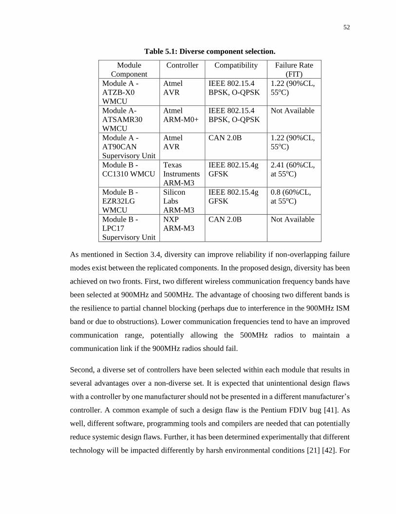
52
Table 5.1: Diverse component selection.
Module
Component
Controller Compatibility Failure Rate
(FIT)
Module A -
ATZB-X0
WMCU
Atmel
AVR
IEEE 802.15.4
BPSK, O-QPSK
1.22 (90%CL,
55oC)
Module A-
ATSAMR30
WMCU
Atmel
ARM-M0+
IEEE 802.15.4
BPSK, O-QPSK
Not Available
Module A -
AT90CAN
Supervisory Unit
Atmel
AVR
CAN 2.0B 1.22 (90%CL,
55oC)
Module B -
CC1310 WMCU
Texas
Instruments
ARM-M3
IEEE 802.15.4g
GFSK
2.41 (60%CL,
at 55oC)
Module B -
EZR32LG
WMCU
Silicon
Labs
ARM-M3
IEEE 802.15.4g
GFSK
0.8 (60%CL,
at 55oC)
Module B -
LPC17
Supervisory Unit
NXP
ARM-M3
CAN 2.0B Not Available
As mentioned in Section 3.4, diversity can improve reliability if non-overlapping failure
modes exist between the replicated components. In the proposed design, diversity has been
achieved on two fronts. First, two different wireless communication frequency bands have
been selected at 900MHz and 500MHz. The advantage of choosing two different bands is
the resilience to partial channel blocking (perhaps due to interference in the 900MHz ISM
band or due to obstructions). Lower communication frequencies tend to have an improved
communication range, potentially allowing the 500MHz radios to maintain a
communication link if the 900MHz radios should fail.
Second, a diverse set of controllers have been selected within each module that results in
several advantages over a non-diverse set. It is expected that unintentional design flaws
with a controller by one manufacturer should not be presented in a different manufacturer’s
controller. A common example of such a design flaw is the Pentium FDIV bug [41]. As
well, different software, programming tools and compilers are needed that can potentially
reduce systemic design flaws. Further, it has been determined experimentally that different
technology will be impacted differently by harsh environmental conditions [21] [42]. For

53
example, different controller technology will have a different apparent activation energy
that results in altered performance at low vs high temperatures. Additionally, different
wireless chips are more susceptible to low ionizing radiation dose rates whereas others are
more susceptible to high dose rates [42]. Therefore, the selection of diverse components
can result in non-overlapping failure mechanisms to reduce the impact of CCFs in a design.
5.1.2 Circuit Simulations
Prior to constructing hardware, key circuit structures have been simulated to verify their
design. Three electronic circuit functions have been selected for simulation:
1) 4-20mA to 0-2.4V sensor interface.
2) RF filtering/matching circuit.
3) Fault detection hardware.
Simulations for the sensor interface and the RF circuit have been completed using
LTSPICE, a free electronic circuit simulator developed by Linear Technology. The fault
detection hardware simulation has been completed using PSPICE, a similar circuit
simulator developed by Cadence. The details for these simulations are presented next.
5.1.2.1 Sensor Interface Simulation
The sensor interface is required to convert a 4-20mA industrial sensor signal into a voltage
for each MCU’s analog to digital converter (ADC). The minimum input voltage for one of
the selected MCU’s is 2.4V. To prevent component damage, a 20mA signal should yield a
voltage of 2.4V to each ADC’s input.
An operational amplifier has been selected to convert the sensor’s current signal into an
appropriately scaled voltage. The schematic for the sensor interface is shown in Figure 5.1.
The results of the simulation can be seen in Figure 5.2. Note that a low sampling frequency
has been selected that simplifies the sensor interface design since WSNs typically do not
require very high sampling frequencies.

54
Figure 5.1: Sensor interface schematic.
Figure 5.2: Sensor interface simulation results.
I1
20m
V1
3.6
R2
8.25K
R3
60
R4
82.5K
R5
82.5K
U1
LT2179A
ADC_High
.dc I1 4m 20m 1m
4mA 6mA 8mA 10mA 12mA 14mA 16mA 18mA 20mA0.4V
0.6V
0.8V
1.0V
1.2V
1.4V
1.6V
1.8V
2.0V
2.2V
2.4V
2.6VV(adc_high)
Current
Volt
age

55
5.1.2.2 RF Filtering Simulation
Module B’s WMCUs are capable of operating across a wide range of sub-GHz radio
frequencies. A RF filter is therefore required to ensure that the radios operates within the
500MHz band. Manufacturer suggested RF filter’s and matching circuits have been used
as the base circuit design and tuned for the 500MHz band. Figure 5.3 to Figure 5.6 show
the schematics and the simulation results for the CC1310 and the EZR32LG WMCU.
Figure 5.3: CC1310 filtering schematic. (Left, TX) (Right, RX).
AC 1
V1
L1
22n
L2
36n
L3
22n
C 1
0.53p
C 2
0.72p
C 3
8.2p
C 4
8.2p
C 5
11p
L4
9n
C 6
160p
C 8
2.1p
L5
49.69n
L6
50.97n
C 9
4.21p
R 1
50
R 4
1C 10
7p
C 11
1.41p
C 12
9.1p
C 13
18p
C 14
9.1p
L7
12n
L8
12n
L9
21.7n
L10
13n
L11
50.97n
C 15
2.10p
L12
49.69n
C 16
4.21p
R 6
472
R 7
1
C 17
1.5p
AC 1
V2
C 18
1p
C 19
7p
C 20
1.41p
C 21
9.1p
C 22
18p
C 23
9.1p
L13
12n
L14
12n
L15
21.7n
L16
13n
C 24
2.10p
L18
49.69n
R 10
50
L17
220n
AC 1.38
V3
R 5
113.4
V4
3.3
L19
22n
L20
36n
L21
22n
C 25
0.53p
C 26
0.72p
C 27
8.2p
C 28
8.2p
C 29
11p
L22
9n
C 30
160p
C 32
2.1p
L23
49.69n
R 8
50
R 14
50
L25
220n
R 13
113.4
V5
3.3
AC 1.38
V6
R 15
472
C 31
1p
R 2
50
R 3
50
C 7
1.5p
C 33
100p
C 34
3.3p
C 35
6.2p
C 36
3.3p
L24
7.5n
L26
7.5n C 37
3.3p
L27
7.5n
C 38
3.3p
L28
7.5n
C 39
100p
L29
18n
R 11
5
C 40
1p
R 12
1
R 16
50
C 41
100p
C 42
3.3p
C 43
6.2p
C 44
3.3p
L30
7.5n
L31
7.5n C 45
3.3p
L32
7.5n
C 46
3.3p
L33
7.5n
C 47
100p
L34
18n
R 18
1
V7
AC 1
C 49
1.14p
V8
AC 1
AC 1
V9
L35
25n
L36
33n
L37
25n
C 50
1p
C 51
1p
C 52
8.2p
C 53
8.2p
C 54
1p
L38
100n
C 55
160p
C 56
2.2p
L39
50n
L40
50n
C 57
4p
R 9
50
R 17
1
R 19
472
C 58
1p
R 20
50
C 59
1.5p
L41
25n
L42
33n
L43
25n
C 61
1p
C 62
1p
C 63
8.2p
C 64
8.2p
C 65
1p
L44
100n
C 66
160p
C 67
2.2p
L45
50n
R 21
50
R 22
50
L46
220n
R 23
110
V10
3.3
AC 1.38
V11
C 60
100p
C 68
3.3p
C 69
6.2p
C 70
2.7p
L47
6.8n
L48
6.8n C 71
3.6p
L49
7.5n
C 72
3.6p
L50
7.5n
C 73
100p
L51
18n
R 24
5
C 74
1p
R 25
1
R 26
50
C 75
330p
C 76
4.7p
C 77
12p
C 78
4.7p
L52
20n
L53
20n C 79
8.2p
L54
15n
C 80
8.2p
L55
15n
C 81
330p
L56
33n
R 27
1Mega
V12
AC 1
C 82
1.14p
V13
AC 0.5
V14
AC 1
L60
0.001n
L61
0.001n
L63
7.5n
C 87
3.6p
C 88
3.6p
R 29
1
L64
7.5n
C 89
100p
R 30
50
C 90
100p
C 91
3p
C 92
6.2p
C 93
2.7p
L65
6.8n
L66
6.8n
L57
500n
L58
500n
C 48
0.1p
C 84
0.1p
V15
AC
1
L59
100n
L67
100n
R 28
50
C 94
3.3p
L62
7.5n
C 85
100p
L68
7.5n
C 86
3.3p C 95
1p
C 96
1p
C 83
330p
C 97
4.7p
C 98
12p
C 99
4.7p
L69
20n
L70
20n C 100
8.2p
L71
15n
C 101
8.2p
L72
15n
C 102
330p
L73
33n
R 32
1Mega
V17
AC
0.5
R 31
50
R F_P R F_N
R X_TX
AN T_OU T
R F_P R F_N
R X_TX
;ac l in 1000 200mega 900mega
.ac l in 1000 200mega 1500mega
C C 1310 TX 500 MH Z
C C 1310 R X 500MH z
AC 1
V1
L1
22n
L2
36n
L3
22n
C1
0.53p
C2
0.72p
C3
8.2p
C4
8.2p
C5
11p
L4
9n
C6
160p
C8
2.1p
L5
49.69n
L6
50.97n
C9
4.21p
R1
50
R4
1C10
7p
C11
1.41p
C12
9.1p
C13
18p
C14
9.1p
L7
12n
L8
12n
L9
21.7n
L10
13n
L11
50.97n
C15
2.10p
L12
49.69n
C16
4.21p
R6
472
R7
1
C17
1.5p
AC 1
V2
C18
1p
C19
7p
C20
1.41p
C21
9.1p
C22
18p
C23
9.1p
L13
12n
L14
12n
L15
21.7n
L16
13n
C24
2.10p
L18
49.69n
R10
50
L17
220n
AC 1.38
V3
R5
113.4
V4
3.3
L19
22n
L20
36n
L21
22n
C25
0.53p
C26
0.72p
C27
8.2p
C28
8.2p
C29
11p
L22
9n
C30
160p
C32
2.1p
L23
49.69n
R8
50
R14
50
L25
220n
R13
113.4
V5
3.3
AC 1.38
V6
R15
472
C31
1p
R2
50
R3
50
C7
1.5p
C33
100p
C34
3.3p
C35
6.2p
C36
3.3p
L24
7.5n
L26
7.5n C37
3.3p
L27
7.5n
C38
3.3p
L28
7.5n
C39
100p
L29
18n
R11
5
C40
1p
R12
1
R16
50
C41
100p
C42
3.3p
C43
6.2p
C44
3.3p
L30
7.5n
L31
7.5n C45
3.3p
L32
7.5n
C46
3.3p
L33
7.5n
C47
100p
L34
18n
R18
1
V7
AC 1
C49
1.14p
V8
AC 1
AC 1
V9
L35
25n
L36
33n
L37
25n
C50
1p
C51
1p
C52
8.2p
C53
8.2p
C54
1p
L38
100n
C55
160p
C56
2.2p
L39
50n
L40
50n
C57
4p
R9
50
R17
1
R19
472
C58
1p
R20
50
C59
1.5p
L41
25n
L42
33n
L43
25n
C61
1p
C62
1p
C63
8.2p
C64
8.2p
C65
1p
L44
100n
C66
160p
C67
2.2p
L45
50n
R21
50
R22
50
L46
220n
R23
110
V10
3.3
AC 1.38
V11
C60
100p
C68
3.3p
C69
6.2p
C70
2.7p
L47
6.8n
L48
6.8n C71
3.6p
L49
7.5n
C72
3.6p
L50
7.5n
C73
100p
L51
18n
R24
5
C74
1p
R25
1
R26
50
C75
330p
C76
4.7p
C77
12p
C78
4.7p
L52
20n
L53
20n C79
8.2p
L54
15n
C80
8.2p
L55
15n
C81
330p
L56
33n
R27
1Mega
V12
AC 1
C82
1.14p
V13
AC 0.5
V14
AC 1
L60
0.001n
L61
0.001n
L63
7.5n
C87
3.6p
C88
3.6p
R29
1
L64
7.5n
C89
100p
R30
50
C90
100p
C91
3p
C92
6.2p
C93
2.7p
L65
6.8n
L66
6.8n
L57
500n
L58
500n
C48
0.1p
C84
0.1p
V1
5
AC
1
L59
100n
L67
100n
R28
50
C94
3.3p
L62
7.5n
C85
100p
L68
7.5n
C86
3.3p C95
1p
C96
1p
RF_P RF_N
RX_TX
ANT_OUT
;ac lin 1000 200mega 900mega
.ac lin 1000 200mega 1500mega
520MHz 540MHz 560MHz 580MHz 600MHz 620MHz 640MHz 660MHz-12mW
-6mW
0mW
6mW
12mW
18mW
24mW
30mW
36mW
42mW
48mW
54mW
-30°
-24°
-18°
-12°
-6°
0°
6°
12°
18°
24°
30°
36° V(rf_p)*I(R31)
390MHz 450MHz 510MHz 570MHz 630MHz 690MHz0mW
3mW
6mW
9mW
12mW
15mW
18mW
21mW
24mW
27mW
30mW
33mW
-840°
-770°
-700°
-630°
-560°
-490°
-420°
-350°
-280°
-210°
-140°
-70° I(R26)*V(ant_out)
Figure 5.4: CC1310 filtering simulation. (Left, TX) (Right, RX).
Frequency Frequency
Po
wer
Po
wer

56
For both sets of simulations, the maximum gain occurs at around 580MHz rather than the
desired 490MHz center frequency in the selected 500MHz band. It is expected that
unmodelled conditions (such as input pin capacitances, trace impedances, and stray
capacitances) will center the signal closer to 490MHz. Therefore, during the PCB
implementation of Module B, a spectrum analyzer has been used to confirm that that the
bandpass signal is shifted closer to 490MHz.
5.1.2.3 Fault Detection Hardware Simulation
In the fault detection hardware simulation, the circuit is expected to detect and identify
digital communication bus faults, such as encoding and ‘stuck-at’ faults. Although the
schematic for this hardware has not been shown, one of the simulations results has be
presented in Figure 5.7. The results for a ‘stuck-at’ fault for a digital communication line
AC 1
V1
L1
22n
L2
36n
L3
22n
C1
0.53p
C2
0.72p
C3
8.2p
C4
8.2p
C5
11p
L4
9n
C6
160p
C8
2.1p
L5
49.69n
L6
50.97n
C9
4.21p
R1
50
R4
1C10
7p
C11
1.41p
C12
9.1p
C13
18p
C14
9.1p
L7
12n
L8
12n
L9
21.7n
L10
13n
L11
50.97n
C15
2.10p
L12
49.69n
C16
4.21p
R6
472
R7
1
C17
1.5p
AC 1
V2
C18
1p
C19
7p
C20
1.41p
C21
9.1p
C22
18p
C23
9.1p
L13
12n
L14
12n
L15
21.7n
L16
13n
C24
2.10p
L18
49.69n
R10
50
L17
220n
AC 1.38
V3
R5
113.4
V4
3.3
L19
22n
L20
36n
L21
22n
C25
0.53p
C26
0.72p
C27
8.2p
C28
8.2p
C29
11p
L22
9n
C30
160p
C32
2.1p
L23
49.69n
R8
50
R14
50
L25
220n
R13
113.4
V5
3.3
AC 1.38
V6
R15
472
C31
1p
R2
50
R3
50
C7
1.5p
C33
100p
C34
3.3p
C35
6.2p
C36
3.3p
L24
7.5n
L26
7.5n C37
3.3p
L27
7.5n
C38
3.3p
L28
7.5n
C39
100p
L29
18n
R11
5
C40
1p
R12
1
R16
50
C41
100p
C42
3.3p
C43
6.2p
C44
3.3p
L30
7.5n
L31
7.5n C45
3.3p
L32
7.5n
C46
3.3p
L33
7.5n
C47
100p
L34
18n
R18
1
V7
AC 1
C49
1.14p
V8
AC 1
AC 1
V9
L35
25n
L36
33n
L37
25n
C50
1p
C51
1p
C52
8.2p
C53
8.2p
C54
1p
L38
100n
C55
160p
C56
2.2p
L39
50n
L40
50n
C57
4p
R9
50
R17
1
R19
472
C58
1p
R20
50
C59
1.5p
L41
25n
L42
33n
L43
25n
C61
1p
C62
1p
C63
8.2p
C64
8.2p
C65
1p
L44
100n
C66
160p
C67
2.2p
L45
50n
R21
50
R22
50
L46
220n
R23
110
V10
3.3
AC 1.38
V11
C60
100p
C68
3.3p
C69
6.2p
C70
2.7p
L47
6.8n
L48
6.8n C71
3.6p
L49
7.5n
C72
3.6p
L50
7.5n
C73
100p
L51
18n
R24
5
C74
1p
R25
1
R26
50
C75
330p
C76
4.7p
C77
12p
C78
4.7p
L52
20n
L53
20n C79
8.2p
L54
15n
C80
8.2p
L55
15n
C81
330p
L56
33n
R27
1M ega
V12
AC 1
C82
1.14p
V13
AC 0.5
V14
AC 1
L60
0.001n
L61
0.001n
L63
7.5n
C87
3.6p
C88
3.6p
R29
1
L64
7.5n
C89
100p
R30
50
C90
100p
C91
3p
C92
6.2p
C93
2.7p
L65
6.8n
L66
6.8n
L57
500n
L58
500n
C48
0.1p
C84
0.1p
V15
AC
1
L59
100n
L67
100n
R28
50
C94
3.3p
L62
7.5n
C85
100p
L68
7.5n
C86
3.3p C95
1p
C96
1p
C83
330p
C97
4.7p
C98
12p
C99
4.7p
L69
20n
L70
20n C100
8.2p
L71
15n
C101
8.2p
L72
15n
C102
330p
L73
33n
R32
1M ega
V17
AC
0.5
R31
50
R33
50
C103
220p
C104
8.2p
C105
15p
C106
5.6p
L74
18n
L75
18n C107
20p
L77
220n
V16
AC 0.5
L79
25n
V18
3.6
C108
2.7p
C109
5.1p
L78
56n
R35
1M ega
C110
220p
C111
8.2p
C112
15p
C113
5.6p
L76
18n
L80
18n C114
20p
L81
220n
L82
25n
V20
3.3
C115
2.7p
C116
5.1p
L83
56n
R36
50
R37
1M ega
V19
AC 0.5
L84
56n
RF_P RF_N
RX_TX
ANT_OUT
RF_P RF_N
RX_TX
;ac lin 1000 200mega 900mega
.ac lin 1000 200mega 1500mega
CC1310 TX 500 M HZ
CC1310 RX 500M Hz
EZR32 TX 500 M HZ
EZR32 RX 500 M HZ
AC 1
V1
L1
22n
L2
36n
L3
22n
C1
0.53p
C2
0.72p
C3
8.2p
C4
8.2p
C5
11p
L4
9n
C6
160p
C8
2.1p
L5
49.69n
L6
50.97n
C9
4.21p
R1
50
R4
1C10
7p
C11
1.41p
C12
9.1p
C13
18p
C14
9.1p
L7
12n
L8
12n
L9
21.7n
L10
13n
L11
50.97n
C15
2.10p
L12
49.69n
C16
4.21p
R6
472
R7
1
C17
1.5p
AC 1
V2
C18
1p
C19
7p
C20
1.41p
C21
9.1p
C22
18p
C23
9.1p
L13
12n
L14
12n
L15
21.7n
L16
13n
C24
2.10p
L18
49.69n
R10
50
L17
220n
AC 1.38
V3
R5
113.4
V4
3.3
L19
22n
L20
36n
L21
22n
C25
0.53p
C26
0.72p
C27
8.2p
C28
8.2p
C29
11p
L22
9n
C30
160p
C32
2.1p
L23
49.69n
R8
50
R14
50
L25
220n
R13
113.4
V5
3.3
AC 1.38
V6
R15
472
C31
1p
R2
50
R3
50
C7
1.5p
C33
100p
C34
3.3p
C35
6.2p
C36
3.3p
L24
7.5n
L26
7.5n C37
3.3p
L27
7.5n
C38
3.3p
L28
7.5n
C39
100p
L29
18n
R11
5
C40
1p
R12
1
R16
50
C41
100p
C42
3.3p
C43
6.2p
C44
3.3p
L30
7.5n
L31
7.5n C45
3.3p
L32
7.5n
C46
3.3p
L33
7.5n
C47
100p
L34
18n
R18
1
V7
AC 1
C49
1.14p
V8
AC 1
AC 1
V9
L35
25n
L36
33n
L37
25n
C50
1p
C51
1p
C52
8.2p
C53
8.2p
C54
1p
L38
100n
C55
160p
C56
2.2p
L39
50n
L40
50n
C57
4p
R9
50
R17
1
R19
472
C58
1p
R20
50
C59
1.5p
L41
25n
L42
33n
L43
25n
C61
1p
C62
1p
C63
8.2p
C64
8.2p
C65
1p
L44
100n
C66
160p
C67
2.2p
L45
50n
R21
50
R22
50
L46
220n
R23
110
V10
3.3
AC 1.38
V11
C60
100p
C68
3.3p
C69
6.2p
C70
2.7p
L47
6.8n
L48
6.8n C71
3.6p
L49
7.5n
C72
3.6p
L50
7.5n
C73
100p
L51
18n
R24
5
C74
1p
R25
1
R26
50
C75
330p
C76
4.7p
C77
12p
C78
4.7p
L52
20n
L53
20n C79
8.2p
L54
15n
C80
8.2p
L55
15n
C81
330p
L56
33n
R27
1M ega
V12
AC 1
C82
1.14p
V13
AC 0.5
V14
AC 1
L60
0.001n
L61
0.001n
L63
7.5n
C87
3.6p
C88
3.6p
R29
1
L64
7.5n
C89
100p
R30
50
C90
100p
C91
3p
C92
6.2p
C93
2.7p
L65
6.8n
L66
6.8n
L57
500n
L58
500n
C48
0.1p
C84
0.1p
V15
AC
1
L59
100n
L67
100n
R28
50
C94
3.3p
L62
7.5n
C85
100p
L68
7.5n
C86
3.3p C95
1p
C96
1p
C83
330p
C97
4.7p
C98
12p
C99
4.7p
L69
20n
L70
20n C100
8.2p
L71
15n
C101
8.2p
L72
15n
C102
330p
L73
33n
R32
1M ega
V17
AC
0.5
R31
50
R33
50
C103
220p
C104
8.2p
C105
15p
C106
5.6p
L74
18n
L75
18n C107
20p
L77
220n
V16
AC 0.5
L79
25n
V18
3.6
C108
2.7p
C109
5.1p
L78
56n
R35
1M ega
RF_P RF_N
RX_TX
ANT_OUT
RF_P RF_N
RX_TX
;ac lin 1000 200mega 900mega
.ac lin 1000 200mega 1500mega
CC1310 TX 500 M HZ
CC1310 RX 500M Hz
EZR32 TX 500 M HZ
Figure 5.5: EZR32LG filtering schematic. (Left TX) (Right RX).
460MHz 500MHz 540MHz 580MHz 620MHz 660MHz0mW
1mW
2mW
3mW
4mW
5mW
6mW
7mW
8mW
9mW
10mW
11mW
12mW
-1.12K°
-1.04K°
-0.96K°
-0.88K°
-0.80K°
-0.72K°
-0.64K°
-0.56K°
-0.48K°
-0.40K°
-0.32K°
-0.24K°
-0.16K° V(n113)*I(R36)
420MHz 480MHz 540MHz 600MHz 660MHz 720MHz-1mW
0mW
1mW
2mW
3mW
4mW
5mW
6mW
7mW
8mW
9mW
10mW
11mW
-1.0K°
-0.9K°
-0.8K°
-0.7K°
-0.6K°
-0.5K°
-0.4K°
-0.3K°
-0.2K°
-0.1K°
0.0K°
0.1K°
0.2K° I(R33)*V(n105)
Figure 5.6: EZR32LG filtering simulation. (Left TX) (Right RX).
Po
wer
Po
wer
Frequency Frequency

57
is shown in the figure. A trip signal is sent after 1 byte of inactivity, or 8 digital pulses
(blue line), for a digital line communicating at 100KHz using the I2C protocol. The trip
signal then triggers a switch that drives current through a relay (red line).
Figure 5.7: Circuit simulation depicting a trip signal for the fault detection
hardware.
5.1.3 PCB Modules
The second step in the hardware implementation process is to develop the PCB prototypes
for the proposed WSN system. This system consists of two dual-redundant modules,
Module A and Module B. Module A has been selected to operate at 900MHz and comprises
of the following components: the ATZB-X0 WMCU, the ATSAMR30 WMCU and the
AT90CAN supervisory unit.
A dual-redundant 4-20mA sensor interface has also been implemented, along with a dual-
redundant digital communication bus (SPI and I2C) and an external wired CAN bus.

58
Electromechanical relays have been used to reconfigure the device if faults are detected
within the various components. The prototype for Module A is depicted in Figure 5.8.
Figure 5.8: Module A PCB prototype.
Module B has been selected to operate at 500MHz and comprises of the following
components: the CC1310 WMCU, the EZR32LG WMCU and the LCP17 supervisory unit.
The similar features to Module A have been included in Module B, and the prototype is
depicted in Figure 5.9.
Figure 5.9: Module B PCB prototype.

59
A prototype for the modularized device has also been built. In the modular design prototype
implementation, each module has been divided into several sub-modules. Module A has
been divided into three sub-modules for its two WMCUs and the supervisory unit, A1, A2
and S1 respectively. Similarly, Module B has been divided into three sub-modules for its
two WMCUs and supervisory unit, B1, B2 and S2 respectively. These sets of sub-modules
are shown in Figure 5.10 to Figure 5.12.
Figure 5.10: Sub-modules A1 (left) and A2 (right).
Figure 5.11: Sub-modules B1 (left) and B2 (right).

60
Figure 5.12: Sub-modules S1 (left) and S2 (right).
The modular design’s auxiliary systems (such as the dual-redundant sensor interface and
fault reconfiguration mechanisms) have been separated into two sub-modules, AUX1 and
AUX 2. The auxiliary sub-modules are shown in Figure 5.13.
Figure 5.13: Sub-modules AUX1 (left) and AUX2 (right).
The proprietary fault detection hardware has also been separated into a sub-module,
which is shown in Figure 5.14.

61
Figure 5.14: Proprietary fault detection hardware sub-module.
The complete modular design is shown in Figure 5.15.
Figure 5.15: Modularized design.
5.2 Software Implementation
Software implementation includes the integration of an operating system (OS) across each
embedded platform, the communication stack and the remote server for data-logging.
The complete software stack for the developed WSN system is illustrated in Figure 5.16.
At the base-layer are the MCU drivers and radio drivers for controlling the software-

62
hardware interactions. The second layer from the bottom is the embedded OS that is
responsible for scheduling tasks, handling interrupts and managing the application. The
third layer is the medium access control (MAC) protocol. The MAC protocol dictates the
flow of data to and from a radio to ensure that the medium (wireless link) is accessed
through some control scheme. The next layer is the network protocol which is responsible
for dictating how data is routed through the network. The top layer is the application and
is the location where the various test algorithms reside.
Figure 5.16: Software stack for implementation.
Above the embedded software stack is the Linux remote server driver and the ThingSpeak
remote server. The Linux remote server driver interacts with the embedded software
through the application layer and is responsible for pushing data to the ThingSpeak server
for data logging. Each of these layers is discussed in more depth.

63
5.2.1 Hardware Drivers
To enable the correct software-hardware interactions on each embedded MCU, a set of
hardware drivers is required. Table 5.2 identifies the hardware driver that have been
developed, the MCUs that required the driver and the functionality provided by the driver.
Table 5.2: Developed microcontroller drivers.
Driver Target MCU Functionality
ADC EZR32HG, EZR32LG, SAMR30,
ATXMEGA, CC1310, AT90CAN,
LPC17, Atmel 8051
Analog to digital conversion for
the 4-20mA sensor interface
I2C EZR32HG, EZR32LG, SAMR30,
ATXMEGA, CC1310, AT90CAN,
LPC17, Atmel 8051
General purpose bus
communication (multi-master)
SPI EZR32HG, EZR32LG, SAMR30,
ATXMEGA, CC1310, AT90CAN,
LPC17
General purpose bus
communication (multi-master)
UART ATXMEGA, SAMR30 Peer-to-peer microcontroller
interfacing
TIMER EZR32HG, EZR32LG, SAMR30,
ATXMEGA, CC1310, AT90CAN,
LPC17, Atmel 8051
Timer and task scheduling
CAN 2.0B AT90CAN, LPC17 CAN bus driver for CAN
transceiver module
Each MCU required drivers for their ADCs, buses (I2C and SPI) and timers. Only the
supervisor units required the CAN 2.0B driver. Only the ATXMEGA and the ATSAMR30
adopted the universal asynchronous receiver-transmitter as an added communication
channel during early prototyping. These drivers represent the lowest layer of the software
stack in Figure 5.16.
5.2.2 Operating System Porting
As noted previously, there are several challenges that arise when working with a diverse
set of MCUs. After evaluating several OSs suitable for WSN devices, RIOT OS has been
selected [43].
Table 5.3 summarizes some of the effort required to port RIOT OS for 8 different MCUs.
Note that RIOT OS could not be ported for the uC8051 architecture, since the CPU core’s
stack in this architecture differs significantly from more modern MCU architectures.

64
Table 5.3: Summary of porting requirements for RIOT OS.
Microcontroller Architecture Port Compiler Port
ATXMEGA Redefine CPU Registers and CPU
Stack Calls. Interrupt Calls
GNU Supported
CC1310 Direct Support LTS Compiler Port - remove atomic
calls, alter data type definition, change
assembly calls
ATSAMR30 Adaption of the ATSAMR20 GNU Supported
EZR32HG Adaptation of the EZR32HG Arm-gcc Port - minor changes to
header support calls, assembly calls
EZR32LG Adaptation of the EZR32HG Arm-gcc Port - minor changes to
header support calls, assembly calls
AT90CAN Adaption of the Atmega1281 GNU Supported
LPC17 Direct Support Arm-gcc Port - minor changes to
header support calls, assembly calls
uC8051 Incompatible - CPU stack does not
support
Incompatible - C51 compiler does not
support assembly use
5.2.3 MAC and Network Layers
The next stack layers in Figure 5.16 is the MAC protocol layer and the Network layer. The
IEEE 802.15.4 protocol has been chosen as the primary MAC protocol for use due to its
wide adoption in industry. Due to the complexity and strict timing of the IEEE 802.15.4
standard, manufacturers provide their own custom implementations for their products. The
MAC protocol and its respective drivers are integrated with the Real Time Operating
System stack layer through various interfacing points in the software. These interfacing
points are the radio driver function calls and callback functions.
A second MAC protocol has been developed for the implementation and used with Module
B. The reasoning for this alternate MAC protocol implementation is to demonstrate that
the proposed system need not be tied to the IEEE 802.15.4 protocol. By using manufacturer
provided radio drivers, the second MAC protocol can be linked into the OS in a similar
way described above.
The next layer in the software stack is the network protocol. The network protocol is
responsible for routing data from end to end in the network. Since the network protocol is
not the primary focus of this work, a static routing table has been used for fixed path data
routing.

65
5.2.4 Application Layer
The application layer of the software distinguishes devices from one another. A device
either acts as a field device, a router or a gateway in the network. Field devices poll their
ADC for sensor data, format the information into a packet and then send this packet towards
the gateway device. Router devices act as intermediate devices between the field devices
and the gateway. These devices only re-transmit received data in the direction of the
gateway. The gateway device acts as the network sink, aggregating the received data and
passing it to an external network. In this application, the external network is the
ThingSpeak remote server. The gateway devices communicate externally to a computer
that then connects to the remote server through an Internet connection. Note that the
application layer also houses the microcontroller-based BIT and the supervisory diagnostic
algorithm.
5.2.5 Remote Server Integration
The final software layers are the Linux drivers and the ThingSpeak remote server.
ThingSpeak is a free platform for IoT data collection, data processing and action control.
Using the HTTP, devices with an Internet connection can push and poll data to/from the
ThinkSpeak’s server. The purpose of the server in this application is to demonstrate the
capabilities for the proposed system to interface with an external network and log data.
A computer acts as an intermediate device between a gateway’s application layer and the
ThingSpeak server. A Python script on the computer acts as the ThingSpeak driver,
formatting the collected data and then pushing it the ThingSpeak server over HTTP.
5.3 Implementation Summary
The implementation phase consisted of two core tasks. First, the hardware for the WSN
has been implemented. This process included the diverse component selection, circuit
simulations and the PCB design. The selection of the diverse components and the
supervisory unit satisfied the failure rate requirements from the analysis in Chapter 3. After,
the software for the WSN has been implemented to allow for the devices to operate as a
WSN system. The software implementation included peripheral drivers, an OS, MAC

66
protocols, a network protocol, and gateway interfacing capabilities to the ThingSpeak
remote server.

67
Chapter 6
6 Redundancy Management System Evaluation
The evaluation of the prototype WSN device has been done using a three-fold process.
First, to better understand the reliability improvement gained through the proposed
redundancy management system, a comparative analysis is performed against existing
commercial WSN products. Next, fault injection testing is used to demonstrate the
proposed system’s fault-tolerance. This testing shows how fault coverage is improved by
the supervisory unit and fault detection hardware, while also showing how CCFs can be
reduced through the modularized and diverse system. Finally, several experimental test
cases are used to demonstrate the WSN’s ability to perform industrial monitoring in an
experimental setting. These evaluations have demonstrated the effectiveness of the
proposed redundancy management system.
6.1 Reliability Analysis
The first evaluation method for the redundancy management system is reliability analysis.
Using the analysis from Chapter 2 and Chapter 3, a model can be developed for a one-
module device and a two-module device. For this evaluation, averaged manufacturer
failure rate data has been used to represent the component failure rates. Two scaling factors
modify the failure rates for harsh industrial environments. First, MIL-HDBK-217 has
scaled the component failure rates to an ambient temperature of 105oC and 165oC. These
temperatures are selected based on estimated temperature in a NPP during an accident
condition [44]. The second scaling term is for the radiation degradation factor that results
under 10Krads of ionizing radiation, chosen based on the same previous accident scenario.
Note that 10Krads has been chosen since some WMCUs can only withstand about 20-
30Krads TID [45]. The environmental conditions from [44] are shown in Table 6.1. A
summary of the failure rates used for the various components are shown in Table 6.2.

68
Table 6.1: Environment within a NPP during normal (N) and accident (A)
conditions.
Operating Environment Temperature oC (Ambient)
Radiation Krad (TID)
Control Building (N) 15-40 < 0.2
Auxiliary Building (N) 1-40 0.01 - 1000
Auxiliary Building (A) 40-160 0.01 - 1000
Loop Compartment (N) 15-40 6000
Loop Compartment (A) 120 - 200 8000
Table 6.2: Failure rates and scaling factors for various components.
Component
Failure
Rate
Estimates
(FIT)
Scaling Factor
AF
(105oC)
Scaling Factor
AF
(165oC)
Radiation
Degradation Factor
Δ𝑘
(10Krad TID)
LiPo Battery* 10000 Not Available Not Available Not Available
Power Converter* 20000 5.0 47.7 0.1408
Wireless
Microcontroller**
1.48 5.0 47.7 0.1026
Supervisory
Microcontroller**
1.22 5.0 47.7 0.0638
Sensor Interface* 20000 5.0 47.7 0.2377
RF Circuitry* 5000 27.6 64.4 0
Digital Bus* 20000 5.0 47.7 0.133
*FIT estimated using MIL-HDBK-217F
**FIT derived from chip manufacturer
To evaluate the performance of the developed devices, a comparative analysis against two
existing WSN platforms, the IRIS mote [46] and the Meshlium Gateway [47], has been
performed. These two systems are assumed to contain the same major device components
and failure rates as the proposed WSN device. Note that the IRIS mote is a simple, non-
redundant system whereas the Meshlium gateway incorporates redundancy. As well, it has
been assumed that a BIT-based redundancy management system exists within the
Meshlium gateway that does not have the proposed supervisory unit or fault detection
hardware. Figure 6.1 shows these two wireless devices.

69
Figure 6.1: IRIS mote (left) and the Meshlium gateway (right) device.
The final parameters required for reliability modelling is the fault coverage, 𝑐, and the
CCF’s 𝛽-factor at each layer of the design. Without experimental data, accurate estimates
for these parameters can be challenging. Rather than arbitrarily selecting values, an
optimistic evaluation of the proposed system has been done. Here, the fault coverage level,
𝑐, is assumed to be one and the 𝛽-factors are assumed to be zero for each of the analyzed
devices, when applicable. That is to say, the system has perfect fault coverage and no CCF
mechanisms introduced into the design. Although these model parameters are unrealistic,
all three systems are being evaluated under the same assumed conditions.
Under these assumptions for the model parameters, Figure 6.2 (for 105oC) and Figure 6.3
(for 165oC) show the reliability for four devices: the IRIS mote, the Meshlium gateway, a
one-module device, and the two-module device. Note that for the latter two, each module
is a dual-redundant design by itself, with its own supervisor.
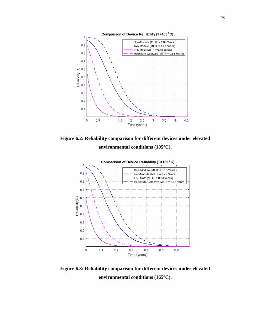
70
Figure 6.2: Reliability comparison for different devices under elevated
environmental conditions (105oC).
Figure 6.3: Reliability comparison for different devices under elevated
environmental conditions (165oC).
Time years
Reliability R
One-Module MTTF ears
Two-Module MTTF ears
IRIS Mote MTTF ears
Meshlium ateway MTTF ears
Time years
Reliability R
One-Module MTTF ears
Two-Module MTTF ears
IRIS Mote MTTF ears
Meshlium ateway MTTF ears

71
From these figures, it is clear that both one-module and two-module devices can provide a
MTTF improvement over the commercially available ones. This result is anticipated since
the proposed system incorporates redundancy within each module and between the two
modules. Nevertheless, this result shows how the proposed topology can improve system
reliability, making it better suited for deployment in harsh environments. Furthermore,
these two figures also clearly demonstrate the impact of harsh environment on system
reliability.
6.2 Fault Injection Testing
The second method for evaluating the developed WSN devices is fault injection testing
[48]. Here, a set of controlled tests are performed on both one-module and two-module
devices to determine whether the systems can tolerate the faults. In these tests, faults are
either emulated within each module through software or are physically injected. Figure 6.4
illustrate these two fault injection methods.
Figure 6.4: Method for injecting faults into a device.
Multiple fault injection tests have been performed on Module A, Module B and their
combination as a two-module device. Dummy sensor data has been used as module inputs,

72
which is then transmitted through any of the module’s radios, as shown in Figure 6.5.
Depending on the specific faults injected, it is expected that a one-module device will fail,
whereas the two-module device should operate successfully.
Figure 6.5: Fault injection test scenario.
Two rounds of fault injection testing have been performed, the first to investigate the fault
coverage improvement, and the second is to evaluate the CCF reduction. For the first round,
the injected faults and the detection location (either the BIT, the supervisory diagnostic
algorithm or the fault detection hardware) are shown in Table 6.3.
As shown in Table 6.3, the microcontroller BIT can detect four of the injected faults. Faults,
such as out-of-bounds outputs (test #1.4) and deadlock/livelock situations (test #1.2 and
test #1.3 respectively) can also be detected by standard software-based BITs. However,
certain faults can only be detected by the supervisory diagnostic algorithm or the fault
detection hardware, which has demonstrated the superiority of the proposed design. As
shown in the table, in test #1.5, digital line noise has been injected into one of the device’s
redundant WMCUs that caused its output value to be changed. The supervisory diagnostic
algorithm has detected a mismatched output between the dual-redundant WMCUs and has
provided feedback to both microcontrollers. Each microcontroller has then compared their

73
intended output value with the received one and has identified that a fault has been induced
by digital line noise. A similar process has occurred in test #1.6, and the supervisory
diagnostic algorithm has been able to help detect the fault successfully.
The fault detection hardware has also contributed to the improvement of fault detection in
a device. The stuck-at faults in test #1.8 and test #1.9 caused a digital communication line
to become unusable. Within a single module, three components share each digital
communication line, preventing BITs from identifying the source of the fault (any
component could have caused the fault). The additional fault detection hardware has been
designed to identify the source of these types of digital communication faults, and therefore
contributes to an improved fault coverage.
Note that the proposed WSN device can still suffer from external faults. For example, if
the sensor inputs faulty data (test #1.5), it cannot be detected by the proposed system. This
can be handled separately, but handling sensor faults are out of the scope of this work.
In a non-redundant WSN devices (such as the IRIS mote in the previous analysis), it is
reasonable to assume that the faults in Table 6.3 could not be detected and recovered from
as they do not employ a redundancy management system. To contrast, existing redundant
WSN devices (such as the Meshlium gateway) might be able to detect faults that are
detected by the microcontroller BIT. However, standard redundant systems that use BITs
cannot detect and recover from the faults that are covered only by the supervisory
diagnostic algorithm or by the fault detection hardware (see Table 6.3).
These tests have demonstrated that additional faults can be detected, and hence, a device’s
fault coverage can be improved by the proposed system. To determine the exact fault
coverage improvement, exhaustive testing has to be done, which is beyond the scope of
this work.

74
Table 6.3: Results of the fault coverage fault injection tests.
Test
#
Faults Injected Location Detected
Microcontroller
BIT
Supervisory
Diagnostic
Algorithm
Fault
Detection
Hardware
Undetected
1.1 WMCU Memory Corruption X
1.2 Deadlock X
1.3 Livelock X
1.4 Out-of-Bounds Output X
1.5 Sensor Input Fault X
1.6 Digital Line Noise X
1.7 Latched Digital Output Register X
1.8 Digital Line ‘Stuck-at’ Fault Low X
1.9 Digital Line ‘Stuck-at’ Fault High X
1.10 Digital Line Encoding Fault X
Totals 4 2 3 1
The second round of fault injection testing has been done to evaluate the impact of CCF
mechanisms in the proposed WSN device. To demonstrate that, faults have been injected
into one-module devices and a two-module device, and the fault-tolerance performance has
been compared, as shown in Table 6.4. Faults have been injected into each module and
into the redundant/diverse sub-systems (i.e., the dual-redundant bus and dual-redundant
sensor interface). In Table 6.4, WMCU A1 Fault represents a complete failure of the
module A’s first redundant wireless microcontroller. If the device is able to complete the
test scenario previously described (acquire dummy data and then send the data through a
radio), then the result of that test is a success and is shown as a ‘pass’ in the table.
Conversely, if the device is unable to complete the test scenario, then the result of that test
is shown as a ‘fail’. Note that in the table, some tests may not be applicable for certain
devices, which are indicated as N/A.
It can be seen from Table 6.4 that the redundant design has reduced certain single points
of failures in the device. Each device has a redundant sensor interface and a redundant
digital bus. A single fault in either of these (test #2.16 to test #2.19) have not caused the
one-module devices or the two-module device to fail.

75
Table 6.4: Results of the CCF fault injection tests.
Test
#
Faults Injected Results (Pass / Fail)
Module A
(One-module)
Module B
(One-module)
Module A+B
(Two-module)
2.1 WMCU A1 Fault PASS N/A PASS
2.2 WMCU A2 Fault PASS N/A PASS
2.3 WMCU B1 Fault N/A PASS PASS
2.4 WMCU B2 Fault N/A PASS PASS
2.5 WMCU A1+A2 Fault FAIL N/A PASS
2.6 WMCU B1+B2 Fault N/A FAIL PASS
2.7 WMCU A1+A2+B1 Fault N/A N/A PASS
2.8 WMCU A1+A2+B2 Fault N/A N/A PASS
2.9 WMCU B1+B2+A1 Fault N/A N/A PASS
2.10 WMCU B1+B2+A2 Fault N/A N/A PASS
2.11 Supervisory S1 Fault PASS N/A PASS
2.12 Supervisory S2 Fault N/A PASS PASS
2.13 Supervisory S1+S2 Fault N/A N/A PASS
2.14 900MHz Channel Blocking FAIL PASS PASS
2.15 500MHz Channel Blocking PASS FAIL PASS
2.16 Sensor Interface S1 Fault PASS PASS PASS
2.17 Sensor Interface S2 Fault PASS PASS PASS
2.18 Digital Bus D1 Fault PASS PASS PASS
2.19 Digital Bus D2 Fault PASS PASS PASS
Totals (Passed) 8 8 19
In certain scenarios, the effect of CCFs have only been mitigated by the diverse, modular
design. For example, in test #2.1 and test #2.2, module A (and therefore module A+B) has
continued to work when any one of module A’s WMCU has suffered from a fault (this is
expected since each module has dual-redundant WMCUs). However, when both WMCUs
within a single module have failed (test #2.5 and test #2.6) only the two-module device has
continued to work. This is because, as designed, the modular device can work if any one
of its modules are operational. Further, the two-module device has continued to work when
only one WMCU (from four WMCUs from module A and B) has been operational (test #
2.7 to test # 2.10). Moreover, partial channel blocking, such as the 900MHz channel
blocking and the 500MHz channel blocking in test #2.14 and test #2.15 respectively, has
been mitigated by the diverse, two-module device.
The fail-safe nature of the supervisory unit has also been demonstrated. The one-module
and two-module devices has continued to operate even when the supervisory unit has
suffered from a loss of function fault (test #2.11 and test #2.12).

76
In summary, in the proposed design, each dual-redundant module has a supervisory unit,
fault detection hardware and reconfiguration mechanisms. If a CCF mechanism causes one
module to fail, the second module in the modularized design does not necessarily fail since
the redundancy management system has also been modularized. Existing WSN devices
might not have this partially-modularized redundancy management system. Therefore, it
would be expected that any failure in their redundancy management system would
constitute a device failure.
6.3 WSN Experimental Test Scenarios
The third evaluation method verifies that the developed devices can effectively perform
industrial WSN monitoring tasks. To do this, the Nuclear Plant Control Test Facility
(NPCTF) has been selected as the test platform. The NPCTF is a physical system that
emulates the main process loops of a CANDU-style nuclear power plant. As such, this
system has an abundant of process variables that can be accessed for monitoring and
control purposes. Figure 6.6 shows the NPCTF system. For this evaluation, the main loop
pressure, denoted as P1, has been selected for monitoring.
Figure 6.6: Nuclear Plant Control Test Facility.
Two test scenarios have been selected. The first test has utilized one-module devices to
measure P1, and then relay this information to a gateway device connected to a remote
server. The second test scenario is similar, except that two-module devices have been used.

77
6.3.1 Test Scenario #1: One-Module Data Trending
The first test scenario demonstrates that a one-module device can be used to create a WSN
system that can collect industrial process data. By relaying information from a field device
to a gateway device, the developed devices can clearly operate together to form a WSN
system. Figure 6.7 and Figure 6.8 show the experimental setup for the three devices using
the NPCTF system.
Figure 6.7: A one-module device interfaced to the NPCTF.
Figure 6.8: Test scenario #1 setup.
In this test, the field device has been programmed to poll the sensor interface on 20 second
intervals for approximately 37 minutes. After each interval, the P1 value has been
forwarded to the gateway device and then uploaded to the ThingSpeak server. The results
for this test are shown in Figure 6.9 and Table 6.5.

78
Figure 6.9: Test scenario #1 ThingSpeak server results.
The results of the test show that the one-module devices achieved an event loss rate of
1.81% and was successfully able to trend the recorded pressure sensor data. The success of
this first test affirms that a one-module device can perform a general industrial WSN
monitoring task.
Table 6.5: Event loss rate results for test scenario #1.
Events Sent Events Received Events Lost Event Loss Rate
112 110 2 1.81%
6.3.2 Test Scenario #2: Two-Module Data Trending
The second test scenario uses a two-module device to complete the described monitoring
task. The interfacing of the modules together is shown in Figure 6.10.

79
Figure 6.10: Interfacing of the two-module device.
The experimental setup using the NPCTF is shown in Figure 6.11. Similar to the previous
test scenario, these devices have been programmed to relay process information to the
gateway devices on 20 second intervals. This test ran for approximately 6 hours over a
three-day span. The results of this test are shown in Figure 6.12 and Table 6.6.
Figure 6.11: Test scenario #2 setup.

80
Figure 6.12: Test scenario #2 ThingSpeak server results.
The results of the second test scenario show an improvement in the event loss rate for the
two-module devices to 0.09%. This improvement is expected since both the 900MHz
module and the 500MHz module can operate simultaneously.
Table 6.6: Event loss rate results for test #2.
Events Sent Events Received Events Lost Event Loss Rate
1093 1092 1 0.09%
Both test scenarios have been successful; information has been relayed from the field
device to the gateway device, and then uploaded to the remote server. This success
concludes the demonstration of the WSN as a general industrial monitoring solution.
6.4 Evaluation Summary
The results of the three evaluation methods have shown the fault-tolerant capabilities of
the proposed redundancy management system. First, the comparative reliability analysis of
the proposed WSN system has shown to increase reliability against existing commercial
devices. Next, the improvement to fault coverage and the reduction in CCF mechanisms
has been shown by the fault injection tests. Finally, the WSN’s ability to complete a general
industrial monitoring tasks has shown that the proposed system can meet the technology’s

81
core requirements. Overall, the evaluation has demonstrated the proposed redundancy
management system’s ability to improve fault coverage and reduce CCFs in a WSN device.
82
Chapter 7
7 Conclusions
In this chapter, this work has been summarized and concluded, along with a list of
contributions.
7.1 Summary
To understand the reliability performance of redundant systems using BITs, first, a
redundancy-relevance boundary has been developed that can be used to identify the
minimum fault coverage level to justify a redundant design. This boundary has then been
extended to include the impact of CCFs. A reliability-improvement plane has also been
developed to determine the reliability improvement gained from a specific design. The
redundancy-relevance boundary and the reliability-improvement plane have been shown
to be a useful tool when analyzing whether a redundant design can potentially improve a
system’s reliability.
Next, a redundancy management system topology has been proposed that uses a
supervisory unit to improve fault detection. By improving the fault detection capabilities
for each BIT, an overall fault coverage improvement can be achieved. This topology has
been extended to form a modularized system design that can help to alleviate the impact of
CCFs. A redundancy management system has then been designed based on the proposed
topology and implemented in a prototype WSN system.
Through reliability analysis and fault injection testing, it has been shown that the proposed
system can effectively alleviate the impact of both imperfect fault coverage and CCFs. The
suitability of the proposed WSN system under an industrial deployment has also been
demonstrated. In summary, the proposed design can be implemented in fault-tolerant WSN
devices to make WSNs more robust to withstand harsh environments.
7.2 Contributions
The contributions are listed as follows:

83
• A reliability-relevance boundary and a reliability-improvement plane has been
developed as a tool to aid in assessing the reliability of a redundant design.
• A redundancy management system topology has been proposed that uses a
supervisory unit to improve fault coverage in a BIT-based design.
• The proposed redundancy management system topology has been extended to form
a modularized system design that can help to alleviate the impact of CCFs.
• Fault detection hardware has been developed for digital communication buses, such
as I2C, that can improve fault coverage.
• The proposed design has been implemented in prototype WSN devices, and the
fault-tolerant performance of the devices has been evaluated.
7.3 Conclusions
A WSN system, when deployed under harsh environment to accomplish a mission, may
experience higher rate of component failure, leading the system to fail prematurely. Fault-
tolerant design based on redundancy can enhance the performance of a WSN system under
such deployments. However, overall system performance improvement can be
compromised due to factors such as imperfect fault coverage and CCFs. The BIT-based
approach for redundancy management suffers from both factors. A BIT-based redundant
WSN system has been designed, developed and investigated that makes use of a
supervisory unit and a modular architecture to address the issues associated with imperfect
fault coverage and CCFs. Based on the evaluation results, it may be concluded that the
combination of a supervisory unit and modular design can potentially alleviate the impact
of both imperfect fault coverage and CCFs on a redundant WSN design, which may to lead
to higher system reliability and fault-tolerance.
7.4 Suggestions for Future Work
To improve upon the existing work, three suggestions are provided to help guide future
work on the proposed redundancy management system:

84
• Evaluate the reliability model developed in Chapter 3 for the supervisory unit
using advanced modelling or experimental testing.
• Complete exhaustive fault injection testing to determine the supervisory unit’s
fault coverage improvement.
• Evaluate the impact of false-positives caused by the redundancy management
system on a device’s reliability.
The reliability model in Chapter 3 (Equation 3.14) used the coverage decay function to
bound the reliability of the proposed redundancy management system. It is not known
whether this model accurately reflects the reliability of the system. However, its accuracy
could be determined by using more advanced modelling techniques (such as dynamic fault
tree analysis) or by completing experimental testing.
It has been shown that the proposed redundancy management system can improve fault
coverage, but the magnitude of the improvement is not yet known. Ultimately, the value of
the redundancy management system hinges on the fault coverage improvement.
Throughout the analysis of the redundancy management system, it has been assumed that
false-positives provided by the supervisory unit can be correctly discerned by each
redundant component’s BIT. Since the supervisory unit is only providing feedback to each
BIT in the proposed design, this assumption might be valid. However, more responsibilities
and decision making could be given to the supervisory unit to further improve fault
coverage. If this is the case, false-positives could be a prominent issue. Further, each BIT
is also susceptible to false-positives. The impact of false-positives from all elements of the
proposed redundancy management should be investigated to conclude how effective the
design is at improving reliability.

85
References
[1] H. M. Hashemian, “Nuclear Power Plant Instrumentation and Control, Nuclear
Power - Control, Reliability and Human Factors,” 2011. [Online]. Available:
http://www.intechopen.com/books/nuclear-power-control-reliability-and-human-
factors/nuclear-power-plantinstrumentation-and-control.
[2] M. Y. Aalsalem, W. Z. Khan, W. Gharibi, M. K. Khan, and Q. Arshad, “Wireless
Sensor Networks in oil and gas industry: Recent advances, taxonomy, requirements,
and open challenges,” Journal of Network and Computer Applications, vol. 113, pp.
87–97, 2018.
[3] H. M. Hashemian, C. J. Kiger, G. W. Morton, and B. D. Shumaker, “Wireless
sensor applications in nuclear power plants,” Nuclear Technology, vol. 173, no. 1,
pp. 8–16, Jan. 2011.
[4] V. Cagri Gungor and G. P. Hancke, Industrial Wireless Sensor Networks:
Applications, Protocols, and Standards. Florida, USA: CRC Press, 2013.
[5] “What is a Wireless Sensor Network?,” National Instrument, White Paper 7142,
2016.
[6] I. Silva, L. A. Guedes, P. Portugal, and F. Vasques, “Reliability and availability
evaluation of Wireless Sensor Networks for industrial applications,” Sensors (Basel,
Switzerland), vol. 12, no. 1, pp. 806–838, Jan. 2012.
[7] Kay Soon Low, W. N. N. Win, and Meng Joo Er, “Wireless Sensor Networks for
industrial environments,” in International Conference on Computational
Intelligence for Modelling, Control and Automation and International Conference
on Intelligent Agents, Web Technologies and Internet Commerce (CIMCA-
IAWTIC’06), 2005, vol. 2, pp. 271–276.
[8] T. Fujiwara and H. Takahashi, Study on a Sensor Network System with a Self-
Maintenance Function for Plant Monitoring System.
[9] N. B. Fuqua, Reliability Engineering for Electronic Design. New York, NY, USA:
Marcel Dekker, Inc., 1987.
[10] S. Battisti, R. Bossart, H. Schönbacher, and M. Van de Voorde, “Radiation damage
to electronic components,” Nuclear Instruments and Methods, vol. 136, no. 3, pp.
451–472, Aug. 1976.
[11] M. Gholami, M. S. Taboun, and R. W. Brennan, “An ad hoc distributed systems
approach for industrial wireless sensor network management,” Journal of Industrial
Information Integration, 2018.

86
[12] A. K. Somani and N. H. Vaidya, “Understanding fault tolerance and reliability,”
Computer, vol. 30, no. 4, pp. 45–50, Apr. 1997.
[13] M. Rausand and A. Høyland, System Reliability Theory: Models, Statistical
Methods, and Applications, Second Edition, vol. 396. 2004.
[14] A. Myers, Complex System Reliability: Multichannel Systems with Imperfect Fault
Coverage. Springer London, 2014.
[15] B. Mihajlovi’c and K. Radecka, “Infrastructure for testing nodes of a Wireless
Sensor Network,” in Handbook of Research on Developments and Trends in
Wireless Sensor Networks: From Principle to Practice, 2010, pp. 79–107.
[16] J. B. Bowles and J. G. Dobbins, “Approximate reliability and availability models for
high availability and fault-tolerant systems with repair,” Quality and Reliability
Engineering International, vol. 20, no. 7, pp. 679–697, 2004.
[17] V. M. Hoepfer, J. H. Saleh, and K. B. Marais, “On the value of redundancy subject
to common-cause failures: Toward the resolution of an on-going debate,” Reliability
Engineering & System Safety, vol. 94, no. 12, pp. 1904–1916, Dec. 2009.
[18] M. L. Shooman, Reliability of Computer Systems and Networks: Fault
Tolerance,Analysis,and Design. New York, NY, USA: John Wiley & Sons,
Inc., 2002.
[19] V. Lakshminarayanan and N. Sriraam, “The effect of temperature on the reliability
of electronic components,” in 2014 IEEE International Conference on Electronics,
Computing and Communication Technologies (CONECCT), 2014, pp. 1–6.
[20] F. Bayle and A. Mettas, “Temperature acceleration models in reliability predictions:
Justification amp; improvements,” in 2010 Proceedings - Annual Reliability and
Maintainability Symposium (RAMS), 2010, pp. 1–6.
[21] U. S. DOD, “Military Handbook, Reliability Prediction of Electronic Equipment,”
MIL-HDBK-217F, 1992.
[22] K. Lauridsen, P. Christensen, and H. E. Kongsø, “Assessment of the reliability of
robotic systems for use in radiation environments,” Reliability Engineering &
System Safety, vol. 53, no. 3, pp. 265–276, Sep. 1996.
[23] Q. Huang and J. Jiang, A Radiation-tolerant wireless monitoring system using a
redundant architecture and diversified commercial off-the-shelf (COTS)
Components, vol. PP. 2018.
[24] “Radiation Effects & Analysis.” [Online]. Available:
https://radhome.gsfc.nasa.gov/radhome/tid.htm. [Accessed: 07-Jan-2004].

87
[25] Z. Gao, C. Cecati, and S. X. Ding, “A survey of fault diagnosis and fault-tolerant
techniques—Part I: Fault diagnosis with model-based and signal-based approaches,”
IEEE Transactions on Industrial Electronics, vol. 62, no. 6, pp. 3757–3767, Jun.
2015.
[26] Z. Gao, C. Cecati, and S. X. Ding, “A survey of fault diagnosis and fault-tolerant
techniques—Part II: Fault diagnosis with knowledge-based and hybrid/Active
approaches,” IEEE Transactions on Industrial Electronics, vol. 62, no. 6, pp. 3768–
3774, Jun. 2015.
[27] C. Bolchini, L. Pomante, F. Salice, and D. Sciuto, “A system level approach in
designing dual-duplex fault tolerant embedded systems,” in Proceedings of the
Eighth IEEE International On-Line Testing Workshop (IOLTW 2002), 2002, pp. 32–
36.
[28] I. F. Akyildiz, W. Su, Y. Sankarasubramaniam, and E. Cayirci, “Wireless sensor
networks: a survey,” Computer Networks, vol. 38, no. 4, pp. 393–422, Mar. 2002.
[29] C. R. Y. Devi, B. Shivaraj, S. H. Manjula, K. R. Venugopal, and L. M. Patnaik,
“EESOR: Energy efficient selective opportunistic routing in Wireless Sensor
Networks,” in Recent Trends in Computer Networks and Distributed Systems
Security, 2014, pp. 16–31.
[30] I. Benkhelifa, N. Nouali, and S. Moussaoui, Disaster Management Projects Using
Wireless Sensor Networks: An Overview. 2014.
[31] Z. Zhao, G.-H. Yang, Q. Liu, V. O. K. Li, and L. Cui, “EasiTest: A multi-radio
testbed for heterogeneous wireless sensor networks,” in IET International
Conference on Wireless Sensor Network 2010 (IET-WSN 2010), 2010, pp. 104–108.
[32] “INTRACOM Defense Electronics.” [Online]. Available:
https://www.intracomdefense.com/cat/160. [Accessed: 12-Sep-2018].
[33] “NuWaves engineering.” [Online]. Available: https://nuwaves.com/system-
sustainment-modernization/range-systems-hardware/. [Accessed: 01-Sep-2018].
[34] D. Mitchell, A. Kulkarni, A. Lostetter, M. Schupbach, J. Fraley, and R. Waits,
“Development and testing of harsh environment, wireless sensor systems for
industrial gas turbines,” no. 48821, pp. 777–784, 2009.
[35] J. Yang, “A harsh environment wireless pressure sensing solution utilizing high
temperature electronics,” Sensors (Basel, Switzerland), vol. 13, no. 3, pp. 2719–
2734, Feb. 2013.
[36] A. Mosleh, K. N. Fleming, G. W. Parry, H. M. Paula, D. H. Worledge, and D. M.
Rasmuson, “Procedures for treating common cause failures in safety and reliability
studies: Analytical background and techniques,” United States, 1989.

88
[37] H. Al-Asaad, B. T. Murray, and J. P. Hayes, “Online BIST for embedded systems,”
IEEE Design Test of Computers, vol. 15, no. 4, pp. 17–24, Oct. 1998.
[38] Li Chen and S. Dey, “Software-based self-testing methodology for processor cores,”
IEEE Transactions on Computer-Aided Design of Integrated Circuits and Systems,
vol. 20, no. 3, pp. 369–380, Mar. 2001.
[39] A. Krstic, and, L. Chen, and S. Dey, “Embedded software-based self-test for
programmable core-based designs,” IEEE Design Test of Computers, vol. 19, no. 4,
pp. 18–27, Jul. 2002.
[40] W. T. Hale and G. M. Bollas, “Design of built-In tests for active fault detection and
isolation of discrete faults,” IEEE Access, vol. 6, pp. 50959–50973, 2018.
[41] D. Price, “Pentium FDIV flaw-lessons learned,” IEEE Micro, vol. 15, no. 2, pp. 86–
88, Apr. 1995.
[42] Qiang Huang, “Investigation of radiation-hardened design of electronic systems
with applications to post-accident monitoring for nuclear power plants,” University
of Western Ontario, 2019.
[43] E. Baccelli, O. Hahm, M. Gunes, M. Wahlisch, and T. C. Schmidt, “RIOT OS:
Towards an OS for the Internet of Things,” in 2013 IEEE Conference on Computer
Communications Workshops (INFOCOM WKSHPS), 2013, pp. 79–80.
[44] K. Korsah and R. T. Wood, “Qualification of microprocessor-based equipment for
nuclear power plant environments,” 2002.
[45] R. Gomaa, I. Adly, K. Sharshar, A. Safwat, and H. Ragai, “Radiation tolerance
assessment of commercial ZigBee wireless modules,” in 2014 IEEE Radiation
Effects Data Workshop (REDW), 2014, pp. 1–5.
[46] “IRIS.” [Online]. Available:
http://www.memsic.com/userfiles/files/Datasheets/WSN/IRIS_Datasheet.pdf.
[Accessed: 10-Oct-2018].
[47] “Meshlium.” [Online]. Available: http://www.libelium.com/products/meshlium/.
[Accessed: 10-Oct-2018].
[48] Mei-Chen Hsueh, T. K. Tsai, and R. K. Iyer, “Fault injection techniques and tools,”
Computer, vol. 30, no. 4, pp. 75–82, Apr. 1997.

89
Curriculum Vitae
Name: Madison McCarthy
Post-secondary University of Guelph
Education and Guelph, Ontario, Canada
Degrees: 2012-2016 B.Eng.
The University of Western Ontario
London, Ontario, Canada
2017-2019 M.E.Sc.
Publications:
M. McCarthy, A. Bari and J. Jiang, “Wireless sensor network reliability for real-time
monitoring in nuclear power plants,” 11th International Topical Meeting on Nuclear Plant
Instrumentation, Control, and Human Machine Interface Technologies (NPIC&HMIT
2019).