design for 3d agility and virtual compliance using
TRANSCRIPT

DESIGN FOR 3D AGILITY AND VIRTUAL COMPLIANCE USING
PROPRIOCEPTIVE FORCE CONTROL IN DYNAMIC LEGGED ROBOTS
A DISSERTATION
SUBMITTED TO THE ROBOTICS INSTITUTE,
SCHOOL OF COMPUTER SCIENCE AT CARNEGIE MELLON UNIVERSITY
IN PARTIAL FULFILLMENT OF THE REQUIREMENTS
FOR THE DEGREE OF
MASTER OF SCIENCE
CMU-RI-TR-16-39
Simon Kalouche
October 2016

c© Copyright by Simon Kalouche 2017
All Rights Reserved
ii

I certify that I have read this dissertation and that, in my opinion, it is fully adequate
in scope and quality as a dissertation for the degree of Master of Science.
(Howie Choset) Principal Adviser
I certify that I have read this dissertation and that, in my opinion, it is fully adequate
in scope and quality as a dissertation for the degree of Master of Science.
(Hartmut Geyer)
I certify that I have read this dissertation and that, in my opinion, it is fully adequate
in scope and quality as a dissertation for the degree of Master of Science.
(H. Benjamin Brown)
Approved for the Carnegie Mellon University Committee on Graduate Studies
iii
”Simplicity is the ultimate sophistication” - Leonardo Da Vinci
iv

Abstract
For legged robots to be effective in real-world scenarios they must be capable of robustly navigating
complex 3D environments using multiple modes of mobility. To achieve mobility over such a broad
set of terrain topographies - spanning structured and unstructured environments - an ideal robot will
employ both static, highly stable motions (e.g. dexterous crawling, climbing, walking), as well as
highly dynamic agility maneuvers (e.g. leaping, inertial reorientation, controlled landing; running;
etc.) to optimally traverse the terrain at hand. Therefore, a capable legged robot must be both
dexterous, for precise footstep placement, and dynamic, for running and jumping when obstacles
are insurmountable by static gaits alone. For example, extra-terrestrial landscapes or a collapsed
rubble environment, ubiquitous to war and disaster zones, will contain regions of highly rugged
yet relatively level ground. In these environments using high bandwidth virtual compliance, made
possible by low impedance actuators, will allow the robot’s legs to actively conform to the terrain
producing a more efficient and swift mode of locomotion as compared to a statically stable crawling
gait which requires accurate terrain mapping and explicit foot step planning. Alternatively if the
terrain is both sloped and rugged it may be ideal to crawl or climb slowly using precise footholds made
possible by dexterous limbs with a large workspace. Likewise, unstructured or collapsed disaster
environments often contain local discontinuities (e.g. cavities, pits, ditches, curbs, obstructions,
large local elevation changes relative to the robots leg length, etc.) in the robot’s path. For these
situations dynamic jumping, controlled inertial re-orientation during flight, and compliant landing
would allow the robot to traverse the otherwise insurmountable obstacle and continue forward with
its mission. This thesis explores the design of a new electromechanically actuated robot with legs
capable of dexterous walking, running, and most significantly, explosive omni-directional jumping
and actively compliant landing. A robot with such capabilities does not yet exist but is needed for
legged robots to make the next leap in real-world effectiveness.
v

Acknowledgments
I would like to thank my adviser, my parents, family, and friends for supporting me through all
my academic and professional endeavors. I would also like to thank all current and past members
of the Biorobotics Lab and other affiliates that I have worked with at CMU. Specifically, a great
deal of thanks is owed to Youshuang Ding who developed the low-level firmware for the custom
motor controllers and was fundamental to the success of this project. Additionally, I would like
to thank Ben Brown, Hartmut Geyer, Dave Rollinson, Matthew Travers, Alex Ansari, Chaohui
Gong, Arun Rangaprasad, Lu Li, Curtis Layton, Matthew Tesch, Florian Enner, Alex Long, Gavin
Kenneally, Ted Kern, and Matt Martone all of whom contributed along the way. This research
was conducted with Government support under and awarded by DoD, Air Force Office of Scientific
Research, National Defense Science and Engineering Graduate (NDSEG) Fellowship, 32 CFR 168a.
vi

Contents
Abstract v
Acknowledgments vi
1 Introduction 1
1.1 Motivation . . . . . . . . . . . . . . . . . . . . . . . . . . . . . . . . . . . . . . . . . 3
1.2 Hypothesis . . . . . . . . . . . . . . . . . . . . . . . . . . . . . . . . . . . . . . . . . 7
1.3 Contribution . . . . . . . . . . . . . . . . . . . . . . . . . . . . . . . . . . . . . . . . 7
1.4 Thesis Outline . . . . . . . . . . . . . . . . . . . . . . . . . . . . . . . . . . . . . . . 8
2 Design Principles for Dynamic Legged Robots 10
2.1 State of the Art in Dynamic Legged Robots . . . . . . . . . . . . . . . . . . . . . . . 10
2.2 Leg Design Principles for Agility . . . . . . . . . . . . . . . . . . . . . . . . . . . . . 14
2.2.1 High Force, High Speed Legs . . . . . . . . . . . . . . . . . . . . . . . . . . . 15
2.2.2 Passive or Active Compliance . . . . . . . . . . . . . . . . . . . . . . . . . . . 17
2.2.3 Robust/Resilient Mechanisms and Structure . . . . . . . . . . . . . . . . . . . 18
2.2.4 Energy Efficiency . . . . . . . . . . . . . . . . . . . . . . . . . . . . . . . . . . 19
2.3 Actuation Principles for Agility and Virtual Compliance . . . . . . . . . . . . . . . . 20
2.3.1 Thermal Specific Torque Density . . . . . . . . . . . . . . . . . . . . . . . . . 21
2.3.2 Proprioceptive Actuation and Sensing . . . . . . . . . . . . . . . . . . . . . . 30
2.3.3 Mechanical Robustness . . . . . . . . . . . . . . . . . . . . . . . . . . . . . . 31
2.3.4 Energy Efficiency . . . . . . . . . . . . . . . . . . . . . . . . . . . . . . . . . . 31
2.4 Actuator Comparison . . . . . . . . . . . . . . . . . . . . . . . . . . . . . . . . . . . 32
2.4.1 DD v. QDD v. GM v. SEA . . . . . . . . . . . . . . . . . . . . . . . . . . . . 32
2.4.2 Experimental Validation of Actuator Properties . . . . . . . . . . . . . . . . . 39
3 Leg Design for 3D Agility 47
3.1 A Novel 3-RSR Leg Topology . . . . . . . . . . . . . . . . . . . . . . . . . . . . . . . 47
3.1.1 Kinematics . . . . . . . . . . . . . . . . . . . . . . . . . . . . . . . . . . . . . 48
vii

3.2 Comparison of 3-DoF Leg Topologies . . . . . . . . . . . . . . . . . . . . . . . . . . . 53
3.2.1 Force Envelope Analysis . . . . . . . . . . . . . . . . . . . . . . . . . . . . . . 54
3.2.2 Workspace Analysis . . . . . . . . . . . . . . . . . . . . . . . . . . . . . . . . 57
3.2.3 Proprioceptive Force Sensitivity Analysis . . . . . . . . . . . . . . . . . . . . 58
3.2.4 Energy Transfer . . . . . . . . . . . . . . . . . . . . . . . . . . . . . . . . . . 59
3.2.5 Summary . . . . . . . . . . . . . . . . . . . . . . . . . . . . . . . . . . . . . . 60
3.3 Mechanical Design of the 3-RSR . . . . . . . . . . . . . . . . . . . . . . . . . . . . . 60
3.3.1 Spherical Knee Joint Design . . . . . . . . . . . . . . . . . . . . . . . . . . . . 62
3.3.2 Hip Design and Actuator Placement . . . . . . . . . . . . . . . . . . . . . . . 64
3.3.3 Foot Design . . . . . . . . . . . . . . . . . . . . . . . . . . . . . . . . . . . . . 64
3.3.4 Mass Budgeting . . . . . . . . . . . . . . . . . . . . . . . . . . . . . . . . . . 65
3.3.5 Finite Element Analysis (FEA) . . . . . . . . . . . . . . . . . . . . . . . . . . 65
3.4 Actuator Requirements for Omni-Directional Jumping . . . . . . . . . . . . . . . . . 66
3.5 Quasi-Direct-Drive Actuator . . . . . . . . . . . . . . . . . . . . . . . . . . . . . . . . 67
3.5.1 Mechanical Design . . . . . . . . . . . . . . . . . . . . . . . . . . . . . . . . . 67
3.5.2 Electrical Design . . . . . . . . . . . . . . . . . . . . . . . . . . . . . . . . . . 68
3.5.3 Actuator Control . . . . . . . . . . . . . . . . . . . . . . . . . . . . . . . . . . 69
3.6 Sensing . . . . . . . . . . . . . . . . . . . . . . . . . . . . . . . . . . . . . . . . . . . 80
3.7 Experiments . . . . . . . . . . . . . . . . . . . . . . . . . . . . . . . . . . . . . . . . . 80
3.7.1 Complete System . . . . . . . . . . . . . . . . . . . . . . . . . . . . . . . . . . 80
3.7.2 Omni-Directional Force Vectoring with Force Plate . . . . . . . . . . . . . . . 81
3.7.3 Omni-Directional Running . . . . . . . . . . . . . . . . . . . . . . . . . . . . 81
3.8 Summary and Design Insights of the GOAT leg . . . . . . . . . . . . . . . . . . . . . 81
4 Proprioceptive Force Control for Dynamic Virtual Compliance 86
4.1 Simple Legged Locomotion Controllers . . . . . . . . . . . . . . . . . . . . . . . . . . 86
4.1.1 SLIP Models . . . . . . . . . . . . . . . . . . . . . . . . . . . . . . . . . . . . 86
4.1.2 Raibert Hopping Controller . . . . . . . . . . . . . . . . . . . . . . . . . . . . 89
4.2 Virtual Model Control for Compliant Dynamic Motions . . . . . . . . . . . . . . . . 91
4.2.1 Virtual Joint Compliance . . . . . . . . . . . . . . . . . . . . . . . . . . . . . 92
4.2.2 Virtual Full Leg Compliance . . . . . . . . . . . . . . . . . . . . . . . . . . . 92
4.2.3 Simulation Model . . . . . . . . . . . . . . . . . . . . . . . . . . . . . . . . . . 93
4.2.4 Experimental Validation . . . . . . . . . . . . . . . . . . . . . . . . . . . . . . 93
4.2.5 Virtual Compliance Experiments . . . . . . . . . . . . . . . . . . . . . . . . . 96
4.2.6 Proprioceptive Foot Force Sensing . . . . . . . . . . . . . . . . . . . . . . . . 100
4.2.7 1-DoF Vertical Hopping . . . . . . . . . . . . . . . . . . . . . . . . . . . . . . 100
5 Conclusion and Future Work 103
viii

Bibliography 105
ix

List of Tables
2.1 Results for a series of actuation tests on 4 types of actuators. All tests were done
using a single axis SRI M2210E torque load cell and all actuators were commanded at
control frequencies of 1kHz. Gear motor bandwidth is especially poor which is most
likely attributed to the large amount of backlash present in the gear train. Higher end
gearmotors with lower backlash can be expected to perform much better than results
obtained here and with a higher bandwidth than SEAs as suggested by theory and
other literature. . . . . . . . . . . . . . . . . . . . . . . . . . . . . . . . . . . . . . . . 46
3.1 Comparison of leg parameters for three different 3-DoF leg topologies. . . . . . . . . 54
3.2 Comparison of performance measures for 3-DoF leg topologies. . . . . . . . . . . . . 60
3.3 Lookup table for six-step square commutation [47]. . . . . . . . . . . . . . . . . . . . 71
4.1 State machine for Raibert hopping controller [6]. . . . . . . . . . . . . . . . . . . . . 90
4.2 Agile Performance Comparison in Dynamic Legged Robots. The bulk of the data
from this table has been tabulated and presented originally by Kenneally et. al in
[12]. The performance specifications of GOAT are added to Kenneally’s table for
purpose of comparison to other dynamic legged machines. We introduce a slightly
different metric however for vertical agility which is just the max jumping height of
the robot’s body and the energy delivered to the body during the jump. DoF is the
degrees of freedom per leg. . . . . . . . . . . . . . . . . . . . . . . . . . . . . . . . . . 98
x

List of Figures
1.1 Goat jumping across a cliff. Source: W.Wayne Lockwood, M.D./Corbis, Britannica. 2
1.2 Boston Dynamics legged robots in 2016 [2]. . . . . . . . . . . . . . . . . . . . . . . . 3
2.1 The current state of art in dynamic legged machines in 2016: 1) Boston Dynamics
(BDI) SpotMini, 2) Penn/Ghost Robotics Minitaur, 3) ATRIAS, 4) RHex and Canid,
5) StarlETH, 6) BDI Spot, 7) MIT Cheetah, 8) BDI Atlas. . . . . . . . . . . . . . . 11
2.2 Common robot leg topologies. The robots shown from left to right include the Raibert
quadruped/monopod [6], BDI Spot [2] and MIT Cheetah [9][38], Boston Dynamics
Big Dog [7], Penn/Ghost Robotics Minitaur [12] and ATRIAS [10], the GOAT leg
with a parallel spatial 3-RSR topology. . . . . . . . . . . . . . . . . . . . . . . . . . . 13
2.3 An infrared image of a motor winding captured by a Flir Thermal Camera. It is
important to select a motor that not only has a high torque density but one that
can sustain that torque over periods of time without overheating. The image shows
temperatures higher than 100oC, therefore to prevent motor burnout thermal man-
agement is necessary. . . . . . . . . . . . . . . . . . . . . . . . . . . . . . . . . . . . . 21
2.4 (a) Flux density in steel saturates at around 2 Tesla where flux densities any higher
than 2 T produce rapidly increasing reluctance and the core looses ability to conduct
flux. (b) Minimizing the air gap decreases magnetic reluctance which increases flux
and flux density. (c) Using teeth and slots in the stator allows magnetic force on the
winding coils to be transferred more effectively to rotor torque while reducing the air
gap. Figure Source: [46]. . . . . . . . . . . . . . . . . . . . . . . . . . . . . . . . . . . 23
2.5 Simplified brushless DC motor cross-section. The copper winding coils are shown by
the gold dots and x’s indicating wire traveling out-of and into the page respectively.
The dotted lines represent the end-turn segments of the coils which do not contribute
to magnetic interaction forces. . . . . . . . . . . . . . . . . . . . . . . . . . . . . . . . 26
xi

2.6 Comparison of actuation strategies with respect to meeting the requirements of var-
ious robot applications including: Dynamic Legged Robots (DLR), Human-Robot
Interaction (HRI), Industrial Robots (IR), Quadrotors/Aerial Robots (QAR), and
Wheeled Robots (WR). An optimal actuator could be determined by maximizing the
area enclosed by the polygon of a weighted web graph. . . . . . . . . . . . . . . . . . 33
2.7 (a) Model of a series elastic actuator with series spring stiffness ks, spring dampening
bs, gear reduction n, and motor rotor inertia Im, (b) is a model of a stiff gear motor,
(c) is a model of a quasi-direct-drive actuator, (d) is a model of a direct-drive actuator.
τm and τl are the motor and load torques for a fixed input and output. . . . . . . . . 36
2.8 Impact of spring stiffness on control bandwidth for series elastic actuators. . . . . . . 37
2.9 Relationship between actuator inertia and spring stiffness on control bandwidth and
impact force. . . . . . . . . . . . . . . . . . . . . . . . . . . . . . . . . . . . . . . . . 37
2.10 The ideal configuration for maximizing reduction of a single-stage planetary gear is
to fix the ring gear, couple the sun gear to the motor input, and the planet carrier to
the output. Circles represent the gear’s pitch radius so teeth are not shown. . . . . . 39
2.11 Actuators configured as (a) Direct drive, (b) quasi-direct-drive (1-stage planetary),
(c) gear motor (2-stage planetary), and (d) Hebi X-5 SEA module in the torque
testing rig. The motor back is fixed directly to a mounting plate and the output of
the actuator is coupled to the 1-axis load cell whose housing is also bolted to the rig. 40
2.12 Experimental torque bandwidth testing for a direct-drive T-motor commanded sinu-
soidal torque trajectories at 20, 70 and 100 Hz. . . . . . . . . . . . . . . . . . . . . . 42
2.13 Experimental torque bandwidth testing for a QDD (T-motor with a 1-stage planetary
gear train) commanded sinusoidal torque trajectories at 20, 30 and 40 Hz . . . . . . 42
2.14 Experimental torque bandwidth testing for a GM (T-motor with a 2-stage planetary
gear train) commanded sinusoidal torque trajectories at 10, 20 and 40 Hz . . . . . . 42
2.15 Experimental torque bandwidth testing for a SEA (Hebi X5-1) commanded sinusoidal
torque trajectories at 10, 20 and 30 Hz. . . . . . . . . . . . . . . . . . . . . . . . . . 43
2.16 (a) DD, (b) QDD, (c) GM, (d) SEA. Rise time, settling time, peak time, overshoot,
and proprioceptive torque sensing accuracy and error are calculated using the follow-
ing step response experiments shown here. . . . . . . . . . . . . . . . . . . . . . . . . 44
2.17 Methodology for actuator selection and design starting from the basic, unmodified
electric motor where torque is the limiting resource. This specific methodology flow
results in robots like StarlETH [11], ATRIAS [10], and BiMASC [21]. . . . . . . . . . 45
2.18 Methodology for actuator selection and design starting from the basic, unmodified
electric motor where torque is the limiting resource. This specific methodology flow
results in robots like MIT Cheetah [9], Penn Minitaur [12], and GOAT, the robot
introduced in this thesis. . . . . . . . . . . . . . . . . . . . . . . . . . . . . . . . . . . 45
xii

3.1 CAD Rendering of a viable quadruped using the GOAT leg topology. . . . . . . . . . 48
3.2 the 3-RSR leg topology decomposed into the individual joints at the hip R1, knee
R2,R3,R4, and ankle R5. Although the mechanism is a 3-RSR the physical realization
of the topology is achieved using a 3-RRRRR where the three knee R-joints intersect
at a single point for an effective mobility equal to that of a spherical joint. . . . . . . 49
3.3 Optimization of link 1 length, l1, for maximum workspace and force production based
on the objective function in eq. 3.5. Here the objective function is scaled to fit the
left y-axis. . . . . . . . . . . . . . . . . . . . . . . . . . . . . . . . . . . . . . . . . . . 50
3.4 Characterization of the joint torques, foot position, foot velocity, and foot force for a
vertical jump. The foot force plot shows force produced by constant hip joint torques
of 5 N-m for an example vertical foot trajectory where all 3 hip angles are the same due
to symmetry. The joint torque plot shows the actuator torques required to produce
a constant 100N for downwards at the foot. For a vertical leg trajectory all 3 joint
angles are the same for each point in the trajectory since the mechanism is symmetric.
For omni-direcitonal force vectoring the joint angles and torques will not be the same. 52
3.5 Kinematic diagrams showing leg parameters (Table 3.1 and joint axes for (a) 3-DoF
prismatic, (b) 3-DoF series-articulated, and (c) 3-DoF 3-RSR Parallel Spatial topologies. 53
3.6 Sagittal-plane force envelope comparison. The y and z axes correspond to the coor-
dinates of the foot in the leg frame. The color contour represents the required torque
from each actuator to produce the defined force wrench at that coordinate (i.e. posi-
tion) in the workspace.(a) and (b) represent forces identical to those described in fig.
3.7. . . . . . . . . . . . . . . . . . . . . . . . . . . . . . . . . . . . . . . . . . . . . . . 55
3.7 Frontal-plane force envelope of the 3-RSR leg as compared to the series-articulated
and prismatic legs. The x and y axes correspond to the coordinates of the foot in the
leg frame. The color contour represents the required torque from each actuator to
produce the defined force wrench at that foot coordinate in the workspace. In (a) the
force generated at the foot follows eq. 3.12, while the foot force in (b) is always -100 N
in the z-direction. (c) shows a simulation of the 3-RSR leg producing a force vectored
in the direction indicated by the orange arrow. The green arrows indicate relative
magnitude of the 3 actuator torques required to produce the desired foot force. For
a vertical foot trajectory & force the 3 green arrows will be equal. . . . . . . . . . . 56
3.8 Workspace volume for the (a) prismatic, (b) series-articulated, & (c) 3-RSR topologies
shown on a quadruped body hiding all but 1 leg. Joint limits used for series-articulated
& prismatic legs are based on the joint limits of the MIT Cheetah & the Raibert Hopper. 57
xiii

3.9 (a) Top view of frontal plane for each leg topology. The contour plot indicates by
color what the proprioceptive sensitivity (i.e. torque in N-m) of each actuator is to
a 1 N force acting on the foot. The coordinate on the plot corresponds to the x,yposition of the foot. (b) Matlab kinematic simulation of each foot topology vectoring
force in an arbitrary direction. . . . . . . . . . . . . . . . . . . . . . . . . . . . . . . 58
3.10 Side view of the sagittal plane for each leg topology. The contour plot indicates by
color what the proprioceptive sensitivity (i.e. torque in N-m) of each actuator is to
a 1 N force acting on the foot. The coordinate on the plot corresponds to the y,z
position of the foot. . . . . . . . . . . . . . . . . . . . . . . . . . . . . . . . . . . . . 59
3.11 Renderings of CAD models for the 3-RSR leg design and actuator modules. . . . . . 60
3.12 Knee joint design showing the 3 revolute joints with intersecting axes. Solidworks FEA
results indicate that stresses as high as 123 ksi are present at the bearing support shaft
of the distal knee segment with a conservative applied force of 300 N and safety factor
of 4. Therefore, this component is machined from medium carbon steel with 125 ksi
yield strength in contrast to most of the other components which are machined from
7075 Aluminum with 73 ksi yield strength. . . . . . . . . . . . . . . . . . . . . . . . . 61
3.13 FEA was conducted on each component and the two other critical components were
determined to be (a) the other extended shaft in the knee (R2) and (b) the ankle
link which connects the foot to the carbon fiber l2 rod. A static analysis was used to
determine the maximum expected force each part could see and those forces ranging
from 75N to 200N were applied in the FEA. . . . . . . . . . . . . . . . . . . . . . . . 62
3.14 Optimization plot showing the relationship between the fixed knee angle and total
hip joint range. . . . . . . . . . . . . . . . . . . . . . . . . . . . . . . . . . . . . . . . 63
3.15 Various mechanical components of the 3-RSR leg including foot, knee, and driven link
l1. . . . . . . . . . . . . . . . . . . . . . . . . . . . . . . . . . . . . . . . . . . . . . . 64
3.16 The Tiger Motor U10 shown here has a large 40 mm gap radius and a lightweight
frame. The T-motor U8, U10, and U12 were determined to have one of the highest
thermal specific torques of any COTS motor (0.42 NmkgCo at rgap = 40 mm) [43]. For
reference the custom MIT cheetah motors have a thermal specific torque of 0.71 NmkgCo
at rgap = 49 mm [9]. . . . . . . . . . . . . . . . . . . . . . . . . . . . . . . . . . . . . 68
3.17 The quasi-direct-drive actuator module driven by a T-motor U10 with a single stage
Matex 1:7 planetary gear stage. . . . . . . . . . . . . . . . . . . . . . . . . . . . . . . 69
3.18 Custom GOAT motor driver configured with a Piccolo TMS320F28069M MCU and
a DRV8301 Bridge Driver which drives 6 N-channel Vishay SUM110N06-05L 60 V
MOSFETs with 175oC temperature limit. . . . . . . . . . . . . . . . . . . . . . . . 70
3.19 The custom Hebi Robotics communications board outfitted with a 32-bit ARM Cortex
processor, Ethernet switch, and SPI port among other I/O ports for prototyping. . . 70
xiv

3.20 (a) is a simple motor model showing torque production for three different phase
alignments of the rotor’s permanent magnet and stator’s electromagnetic fields. (b)
shows a decomposition of magnetic force or pull direction into two components: one
that produces torque and one that pulls outward and wastes energy. The purpose of
FOC is to continuously apply a magnetic field in the stator windings which converts
all the magnetic force into the component that produces torque. (c) shows the phase-
shift that exists between phase winding voltage and phase current, which is around
20o here. (d) shows the commanded voltage sinusoids vs. electrical angle and the
corresponding magnetic field produced by the energized windings. Figure source: [56]. 72
3.21 (a) is a flow chart showing the FOC commutation. (b) is the control strategy which
minimizes Id and maximizes Iq. Figure source: [56]. . . . . . . . . . . . . . . . . . . 73
3.22 Representation the input (a, b, c) winding reference frame and the rotating d−q frame
for a 4-pole brushless motor. . . . . . . . . . . . . . . . . . . . . . . . . . . . . . . . . 73
3.23 Output of the RMS current limiter which monitors the RMS current and saturates
the commanded output torque when necessary to remain within the motor winding’s
thermal limits. . . . . . . . . . . . . . . . . . . . . . . . . . . . . . . . . . . . . . . . 75
3.24 Thermal analysis showing the time response in winding temperature to 4 commanded
torques ranging from 1.19 N-m to 2.85 N-m with associated thermal time constants.
Thermal time constant was calculated by 63% of the time taken to reach steady-state.
If steady state was not reached the maximum temperature was used. A FLIR E40
Infrared Thermal Imaging Camera was used to collect real-time temperature data on
the windings. . . . . . . . . . . . . . . . . . . . . . . . . . . . . . . . . . . . . . . . . 76
3.25 A FLIR E40 Infrared Thermal Imaging Camera was used to observe the temperature
gradient over the motor windings and the PCB containing the motor driver FET
bridges. (a) is a top-view IR image of the torque test rig with the motor driver PCB
(cursor 1) and the T-motor (cursor 2). (b) shows a closer view of the T-motor U10.
The thermal image depicts which stator winding poles are being energized and the
temperature at those windings. . . . . . . . . . . . . . . . . . . . . . . . . . . . . . . 76
3.26 Schematic wiring diagram of the electronics for a single GOAT actuator. . . . . . . . 78
xv
3.27 A torque vs current plot of the motor shows the torque constant to be 0.072 N−mA . The
magnetic flux in the motor core begins to saturate at 70 A and the thermal limits of
the motor driver half-bridges reach their thermal limits between 75-80 A. The shaded
color zones indicate allowable duty time and duration of holding torque. The green
region indicates infinite holding as this region is within the continuous current and
thermal limits of the motor; green-yellow corresponds to duty times ranging from
5 minutes to 20 seconds; yellow indicates short duty cycles of up to a few seconds;
orange indicates duty cycles less than 1 second; and red indicates peak instantaneous
torques with a duty cycle of a few milliseconds. . . . . . . . . . . . . . . . . . . . . . 79
3.28 Torque calibration to determine the relationship between the commanded value in the
custom motor-controller Matlab API. . . . . . . . . . . . . . . . . . . . . . . . . . . . 79
3.29 Data from the 6-axis force-torque load cell was collected to determine the ground
reaction forces generated at the foot of the robot. The commanded and actual forces
are presented. The data shows that the leg can produce equal forces along all vectors
of the frontal plane (i.e. any combination of Fx and Fy within the actuators limits).
This corresponds with the analytical data presented in Figs. 3.6 and 3.7. . . . . . . . 82
3.30 Passive landing tests were performed using 3 COTS torsion springs (ks = 4.11N−mrad )
in the 3 hip R-joints. The left image shows resting knee-below-hip position while the
right image shows the 3-RSR knee-above-hip configuration absorbing energy upon
landing. . . . . . . . . . . . . . . . . . . . . . . . . . . . . . . . . . . . . . . . . . . . 82
3.31 GOAT Leg prototype with T-motor U10 actuators mounted in direct-drive configu-
ration. . . . . . . . . . . . . . . . . . . . . . . . . . . . . . . . . . . . . . . . . . . . . 83
3.32 GOAT Leg prototype and experimental 1-DoF vertical jumping test bed. Electronics
and power (LiPo battery — blue) are both shown in the bottom right image off-board,
as tested. The gray ground plate the robot is standing on is a 6-axis force-torque load
cell. . . . . . . . . . . . . . . . . . . . . . . . . . . . . . . . . . . . . . . . . . . . . . 84
4.1 Spring-loaded inverted pendulum (SLIP) model with spring stiffness k and nominal
leg length l0 for (a) a 1-DoF hopper and (b) a 2-DoF hopper [61]. . . . . . . . . . . . 88
4.2 Leg model for the Raibert hopper parallel controller. . . . . . . . . . . . . . . . . . . 90
4.3 MATLAB SimMechanics model of the 3-DoF, 3-RSR leg being simulated for 1-DoF
hopping and compliant landing. . . . . . . . . . . . . . . . . . . . . . . . . . . . . . . 94
4.4 Calibration curves for the impedance controller based on gain scheduling. The impedance
controller is based takes a position error and desired torque as inputs and outputs a
position gain which generates the commanded input torque. . . . . . . . . . . . . . . 95
4.5 Schematic of the hopping control architecture using virtual model control to virtually
emulate a mechanical spring/damper. This allows the leg to compliantly absorb the
impact during touchdown/landing. . . . . . . . . . . . . . . . . . . . . . . . . . . . . 95
xvi

4.6 Experimental results using impedance controller based on continuous gain scheduling.
The position error increases linearly with time but the commanded torque trajectory is
non-linear (sinusoidal). Any arbitrary torque trajectory can be chosen; the continuous
gain scheduler will modulate the gain based on the desired torque and the current
position error. The torque trajectory is followed within 10% error by the direct-drive
actuator at a bandwidth greater than 200 Hz. . . . . . . . . . . . . . . . . . . . . . . 97
4.7 High jump experiments with the GOAT leg delivering 20.11 J of energy to produce a
maximum jump height of 82 cm which is more than double the body height. For Full
video: https://www.youtube.com/watch?v=n319xVomJTQ . . . . . . . . . . . . . . 97
4.8 Experiments were conducted to compare (from left to right) 1) physical joint com-
pliance using mechanical torsion springs in each of the three hip joints without any
motors, 2) virtual joint compliance where motors are used to emulate torsion springs
of various stiffness in the hip (no physical springs), and 3) virtual full leg compliance
where motors are used to emulate the forces of a spring-damper connecting the hip
to the foot (no physical springs). Virtual component placement is shown in blue. . . 99
4.9 Experiments using 3 different virtual spring stiffness’ and dampening coefficients and
observing the response upon landing. The top two plots have virtual joint compliance
with stiffness of 18 and 36 Nm/rad while the bottom plot has a full leg virtual rectified
spring stiffness of 250 N/m and dampening of 10 N-s/m. The response for the whole
leg compliance is ideal with the shown parameters. . . . . . . . . . . . . . . . . . . . 99
4.10 To determine the accuracy of the proprioceptive sensing of foot forces through motor
current the actuator torque feedback is plugged into eq 4.33 to calculate the foot force.
This calculated proprioceptive foot force is then compared to the ground truth from
the 6-axis force-torque plate. The data shown here is from a jump/land experiment
with virtual whole leg compliance with stiffness of 400 N/m and dampening of 15
N-s/m. . . . . . . . . . . . . . . . . . . . . . . . . . . . . . . . . . . . . . . . . . . . . 101
4.11 Data from a second test showing proprioceptive foot force sensing accuracy during a
jump/land experiment. . . . . . . . . . . . . . . . . . . . . . . . . . . . . . . . . . . . 102
4.12 GOAT leg performing continuous 30 cm hopping at 1.5 Hz on a 1-DoF test rig. . . . 102
xvii

Chapter 1
Introduction
With the advent of modern machinery society has benefited tremendously in the transportation
of people and materials. Machines like boats, trains, cars, and planes have all been invented to
overcome the inherent speed and distance limitations of humans. While these conventional vehicles
have enabled us to travel the globe more efficiently, they still require some degree of infrastructure
and are incapable of directly accessing many of Earth’s most isolated and elusive locations where
sure-footed animals roam freely.
As man-kind pushes the barriers of exploration further to extra-terrestrial lands where flat terrain
is sparse and the atmosphere is drastically less dense, conventional wheeled vehicles and aircraft lose
much of the utility they have here on Earth. Thus, an exhaustive exploration of these impassable
environments requires an alternative approach in design – an approach to which we can turn to
biology for inspiration.
For example, the mountain goat (Oreamnos americanus) is notorious for its awing mobility in
seemingly untraversable terrains. This legged mammal exhibits unmatched multi-modal mobility to
scale steep, mountainous and cliff-like terrains – often using its dexterous limbs to precisely position
its feet and toes, maintaining static balance on cliffs with a narrow base of support. Between
instances of static stability the mountain goat exhibits intervals of highly dynamic and powerful
jumping maneuvers to change elevation or reach locations unreachable by statically stable motions
alone. In addition to climbing trees, rocks, and cliffs, the mountain goat is capable of jumping up
to 12 feet in a single leap, running up to 15 mph and paddle swimming in bodies of water [1]. This
form of multi-modal mobility is unsurpassed and remains greatly unmatched by conventional land
vehicles. Therefore, for decades scientists and researchers have turned to biology and specifically
cursorial creatures for inspiration in designing more competent and agile machines.
As humans and animals subconsciously move through the world with our inherent finesse we
often overlook the complexity of mobility and the lengthy evolutionary process which has afforded
us these abilities that we still do not fully comprehend. Therefore, this thesis is a stepping stone
1

CHAPTER 1. INTRODUCTION 2
Figure 1.1: Goat jumping across a cliff. Source: W.Wayne Lockwood, M.D./Corbis, Britannica.
in the arduous endeavor to create machines with mobility matching and exceeding that of their
mammalian cursorial counterparts.
There is still much progress to be made in transforming the current state-of-art in legged robots
from research projects, operating in controlled environments, to deployable and robust platforms
with real-world utility and mobility that approaches that of humans and animals. The most notable
progress in legged robots deployed in unstructured, real-world, environments is demonstrated by
recent videos released by Boston Dynamics. These robots include Atlas, BigDog, Spot and the
all electric SpotMini shown in Fig. 1.2 [2]-[4]. These videos show both biped and quadruped,
hydraulically and electrically actuated, robot’s navigating everything from forested landscapes to
confined spaces and staircases in warehouses and residential environments [4]. However, as control,
autonomous balancing, and legged motion planning algorithms continue to progress the largest
barrier preventing these machines from reaching real-world utility continues to be 1) multi-modal
mobility using force control to interact compliantly with the world like humans and animals; and
2) power efficiency to ensure tasks with reasonable durations can be executed without the need for
manual recharging or external power supplies or tethers.
Specifically, this dissertation is geared towards the development of a new leg topology and ac-
tuation paradigm which will enable legged machines to use proprioceptive force control to exhibit
multi-modal 3D agility through both static and highly dynamic motions. This work discusses design
concepts, actuation principles, implementation details, mathematical analysis, and control strategies
for achieving a new level of 3D agility and active compliance in dynamic legged robots that hopefully
one day will be adept for exhaustive exploration of extra-terrestrial worlds.

CHAPTER 1. INTRODUCTION 3
Figure 1.2: Boston Dynamics legged robots in 2016 [2].
1.1 Motivation
It is estimated that nearly 50% of Earths landmass is currently inaccessible to wheeled or tracked
machines [6]. Humans and animals, however, are readily able to access most of these areas and it is
desirable that robots and machines be able to do the same. Biologically inspired robots, specifically
legged robots, offer enhanced mobility in these impassable environments in situations where it is
unsafe or unfeasible for humans to travel. Although there exist dozens of promising legged robots
today, most are limited dynamically and all make significant trade-offs between efficiency, dexterity,
and dynamic mobility [7]-[16]. Thus, there are still open questions pertaining to leg topology and
actuation schemes which best optimizes performance across the efficiency, dexterity, and dynamic
mobility spectrum.
For legged robots to be effective in real-world scenarios they must be capable of robustly nav-
igating complex 3D environments using multiple modes of mobility. To achieve mobility over such
a broad set of terrain topographies - spanning structured and unstructured environments - an ideal
robot will employ both static, highly stable motions (e.g. dexterous crawling, climbing, walking),
as well as highly dynamic agility maneuvers (e.g. leaping; compliant landing; running; etc.) to
optimally traverse the terrain at hand. Therefore, a capable legged robot must be both dexterous,
for precise footstep placement, and dynamic, for running and jumping when obstacles are insur-
mountable by static gaits alone. For example, extra-terrestrial landscapes or a collapsed rubble

CHAPTER 1. INTRODUCTION 4
environment, ubiquitous to war and disaster zones, will contain regions of highly rugged yet rela-
tively level ground. In these environments using high bandwidth virtual compliance, made possible
by low impedance actuators, will allow the robot’s legs to actively conform to the terrain producing
a more efficient and swift mode of locomotion as compared to a statically stable crawling gait which
requires accurate terrain mapping and explicit foot step planning. Alternatively if the terrain is both
sloped and rugged it may be ideal to crawl or climb slowly using precise footholds made possible by
dexterous limbs with a large workspace. Likewise, collapsed war and disaster zones often contain
local discontinuities in the robot’s path. For these situations dynamic jumping, controlled inertial
re-orientation during flight, and controlled landing would allow the robot to traverse the otherwise
insurmountable obstacle and continue forward with its mission. To accomplish this range of mobility
the conventional pure position based control method will not be adequate. Thus, machines must be
designed to enable both accurate position and force control working in parallel.
The real utility of legged robots is in traveling to locations that are not safe or hard to reach by
humans. These areas of interest are characterized by:
1. Highly unstructured terrains, that are often impassible to wheeled vehicles and currently ex-
isting legged robots;
2. Obstacles of large and steep variations in ground elevation (relative to the robots height)
creating discontinuous paths for walking (i.e. theres a limit to the slope of a terrain that can
be walked over which is around 45 degrees for humans);
3. Pits, holes, ditches and local cavities which also create discontinuities in a walking path;
4. Tight and compact spaces where turning or reorienting to then walk or jump is not possible
or ideal
5. Long distance missions over diverse terrains where different gaits or modes of locomotion can
improve both mobility, efficiency, and longevity.
Legged robots utilize a variety of leg topologies and actuation strategies to enable mobility
over such a large set of terrains. However, the most prominent, currently existing dynamic legged
robots (SpotMini [4], MIT Cheetah [9] [4], ATRIAS [10], Minitaur [12], etc.) shown in Fig. 2.1,
share a fundamental shortcoming that constrains the leg’s most powerful actuators, force producing
capability, and thus dynamic mobility, to the robots sagittal plane. Sagittally constrained and 2.5D
dynamic motions severely inhibit a robots mobility in real-world, complex, 3D environments. For
instance, in tight spaces with discontinuous walking paths, current robots would be required to turn
in place to face a desired heading and then walk or jump forward over/onto an obstacle. This is
less ideal than simply moving or jumping in the direction of the desired heading without having
to reorient the body first. Another scenario is in any human environment where omni-wheels are

CHAPTER 1. INTRODUCTION 5
currently used but limited by steps, cables on the ground, etc. In these environments an omni-
directional legged robot would be capable in terms of mobility. In other words, currently existing
dynamic robots exhibit exceptional mobility in the forward walking and running direction but are
rather unexceptional at running and jumping sideways, diagonally, or backwards. This limitation
is a direct consequence of the current leg topologies and designs being researched, explored, and
developed.
In addition to limited mobility in the full space of SE(3) today’s dynamically capable legged
robots use leg topologies with Jacobians characterized by an unequal distribution of torque require-
ments across the leg’s actuators needed to produce adequate foot forces for running and jumping.
This characteristic of leg design yields unused resources (i.e. actuators) while simultaneously de-
manding extreme performance from other actuators. An ideal leg design would equally distribute
loads across all actuators to avoid wasting resources while reducing system mass and minimizing the
potential of damaging over-burdened components.
If a leg topology burdens one actuator with the majority of the load for running, walking, and
jumping that actuator must have sufficient torque and speed to do so. The most common method of
achieving the required torque is via a transmission which allows the abundant resource of speed in
electromagnetic actuators to be converted to torque, a more limited resource. While transmissions
such as gears, belts, pulleys, and linkages can multiply an actuators torque, they introduce undesired
complexities such as backlash, friction, and other modeling non-linearities all of which contribute to
a system’s mechanical impedance [17]. Mechanical impedance is the inverse of force transparency,
thus a challenge becomes imminent as one goes about designing a machine with sufficient torque
for dynamic motions yet high force transparency (i.e. low impedance) for utilizing force control to
compliantly interact with the surrounding environment.
For effective high-speed traversal through unmapped, unstructured environments a robot must
be able to efficiently deliver energy and absorb impacts from jumping and landing. To address this
requirement many researcher’s have designed robot’s with inherent, built-in, mechanical compliance
using pneumatics, series-elasticity, leaf springs, and bow-legs [6][10][19]. While this inherent compli-
ance is advantageous in protecting actuator transmissions and passively conforming to uncertainties
in the environment, mechanical compliance undesirably:
1. imposes limits on actuation bandwidth;
2. fixes a single mechanical spring and dampening coefficient to the leg which is typically tuned to
a single specific running speed or ground stiffness and not optimal in general for all situations
[21];
3. requires large and inefficient mechanisms to achieve variable mechanical stiffness [21];
4. introduces control complexities when attempting to accurately model the compliance which is
often non-linear [22][24].

CHAPTER 1. INTRODUCTION 6
Therefore, to address the requirement of absorbing and delivering energy while avoiding the issues
associated with mechanical compliance, the ability of a robot to virtually mimic the role of a me-
chanical spring and damper becomes very desirable. This ability can be accomplished using high
fidelity virtual model control. Virtual model control is force-control based frame-work in which a
robot’s actuators can be used to emulate the dynamics of mechanical components such as springs and
dampers [25]. Virtual model control affords a robot the ability to tune leg stiffness and dampening,
in real-time, to be optimal for any terrain or running speed [25].
High fidelity virtual model control, which reacts to disturbances on the millisecond time-scale,
requires high bandwidth, high accuracy, force sensing and control. A common approach to achieve
this level of force control has been to use series-elastic actuators (SEAs) or place a load cell, force
sensor, or strain gauge at the end-effector which directly interacts with the world (i.e. the foot
for legged robots). Using SEAs for force control can work but it associated with the previously
mentioned limitations when inherent mechanical compliance is built-in to the system dynamics. For
dynamic legged robots it is also disadvantageous to place a sensor distally at the foot to measure
ground reaction forces required for virtual model control. This is because 1) adding distal mass
(from a load cell) the to the leg will increase limb inertia which reduces limb acceleration hindering
high speed dynamics and 2) foot impact forces reach multiple times the robot’s total weight and are
cyclic by nature of hopping and running which ultimately requires a challenging level of robustness
and longevity or decreases sensor lifetime. Therefore, it is ideal to use sensors that are 1) proximal
to the body, 2) not in direct contact with the environment (for increased longevity), and 3) capable
of high bandwidth sensing.
A solution that addresses these three criteria is measuring motor torque via motor current and
using the leg Jacobian to transform measured joint torques into an estimate of the force-torque
wrench at the foot (i.e. the ground reaction force). This approach requires no distal sensors, does
not put the sensor directly in the contact load path, and is capable of very high bandwidth sensing.
However, using joint torque to estimate foot force has its own set of design requirements. For motor
current to be a good indicator of joint torque and similarly for joint torque to be a good indicator of
foot force the entire leg design (actuators, joints, linkages, structure, etc.) must have extremely low
mechanical impedance and high force transparency [17][26]. This means the design of every element
in the leg must minimize mass, friction, stiction, inertia, reflected inertia, compliance, and backlash.
This last and most cumbersome requirement negates the use of nearly all transmission devices
which introduce one or more of the listed impedance sources. Additionally, intelligent selection
of leg topology plays an important role in minimizing actuator torque requirements to allow for
minimal use of transmissions [26]. The design methodology used for the creation and synthesis of
the GOAT leg as well as other dynamic robot legs is shown in Fig. 2.17 and 2.18.
With the motivation set, the purpose of this thesis is to describe how to address these design
requirements with the initial task of delivering and compliantly absorbing large 3D forces using
CHAPTER 1. INTRODUCTION 7
robotic limbs and the ultimate goal of improved real-world mobility and utility of legged robots.
1.2 Hypothesis
Considering the initial task of efficiently delivering and absorbing the energy from large 3D forces
using a robot’s limbs, this thesis explores the following hypothesis:
A task-optimized parallel 3-DoF leg topology can allow a robotic leg to be dynamic in 3 dimensions
while also affording it the ability to use direct-drive actuation — with accurate proprioceptive force
sensing — for achieving high fidelity virtual compliance all while maintaining mechanical robust-
ness, low limb inertia, and a usable workspace for agile legged locomotion. This complimentary
combination of leg topology and actuation will produce a robot with unparalleled 3D agility.
This hypothesis considers and addresses the fact that traditional parallel mechanisms have a very
limited workspace that would typically not be adequate for legged locomotion. It also addresses
mechanical robustness in the case of the Delta robot which does have a fairly decent workspace for a
parallel mechanism but is notoriously known for being incapable of bearing or delivering large end-
effector loads which are pervasive in legged locomotion. The following chapters of this dissertation
work toward a validation of the hypothesis stated above.
1.3 Contribution
While this thesis explores the full design methodology used to conceive a completely new leg topology
designed for 3D agility, the main contributions of this work include:
1. detailing the synthesis, mechanical design, analysis, characterization, optimization, and phys-
ical realization of the 3-RSR parallel leg topology enabling omni-directional force and accel-
eration vectoring.
2. an exhaustive survey and trade-off analysis, which illuminates the competing design objectives
that a designer should consider when designing task specific robotic legs with complimentary
topologies, actuation strategies, and control schemes.
3. the successful demonstration — on real hardware — of a mechanically robust 3-DoF, 3-RSR
leg performing: a) explosive jumping and landing using high fidelity virtual model control and
b) high-speed omni-directional running and jumping trajectories while mounted on a test rig.
This thesis introduces and develops GOAT, the gearless omni-directional acceleration-vectoring
topology. GOAT is a novel 3-DOF, parallel 3-RSR leg topology with an optimized workspace

CHAPTER 1. INTRODUCTION 8
driven by an ultra low-impedance actuation scheme for precisely ‘feeling’ forces and dynamically
reacting to the full 3D world around it. This 3-RSR topology expands the multi-modal mobility
of dynamic legged robots beyond operating dynamically in the sagittal plane by enabling explosive
omni-directional jumping, running, and dexterous crawling. The 3-RSR topology puts all 3 of its
actuators in parallel to reduce torque requirements on any one actuator which allows the direct-drive
and quasi-direct drive actuation scheme — which simplify the implementation of high fidelity virtual
model control — to be used.
The 3-RSR leg is optimized for maximum kinematic workspace, force envelope, and energy
delivery/absorption. It is mechanically designed using finite element analysis (FEA) to be robust
and resilient to large 3D impact forces, pervasive in dynamic legged locomotion. Furthermore, the
new leg topology is characterized with respect to multi-modal mobility, specifically 3D jumping via
omni-directional force vectoring, as compared to conventional leg designs.
In addition to leg design and characterization I present an elaborate trade-off analysis and survey
on actuator design principles for dynamic legged robots that achieve a balance of high torque density,
high force transparency (i.e. low mechanical impedance) for high fidelity proprioceptive force control,
and energy efficiency. By designing with control simplicity in mind, using a novel leg-topology
with state-of-the-art actuators, I aim to conceive a new highly dynamic and agile robot capable of
unprecedented 3D agility.
1.4 Thesis Outline
Chapter 2 of this thesis discusses design principles for engineers and researchers looking to understand
and build agile legged machines. A comprehensive survey of existing robots is presented and the
design trade-offs associated with competing goals in legged agility are discussed and clarified. The
two high-level design paradigms discussed are selection, synthesis, and mechanical realization of leg
topology and actuator design, selection, and low-level control for maximizing performance in the
context of legged agility.
Chapter 3 introduces the novel GOAT leg, provides an explanation of the kinematics, presents
several design optimizations to maximize workspace and force envelope, and details the mechanical
design and finite element analysis for high force 6-axis loading. Chapter 3 then compares the GOAT
3-RSR leg topology to other existing 3-DoF leg topologies across several metrics important to legged
robots and legged agility. The mechanical, electrical, and low-level control design of the dynamic
direct-drive and quasi-direct-drive actuator modules are then presented. Chapter 3 concludes with a
calibration and preliminary experimental results for the high fidelity impedance control of GOAT’s
custom actuators.
Chapter 4 presents the control architecture for active virtual compliance in dynamic locomotion
using proprioceptive force control. I provide an overview of important existing dynamic models and

CHAPTER 1. INTRODUCTION 9
control frameworks for compliant and dynamic legged locomotion including SLIP and the Raibert
controller. The bulk of chapter 4 is concerned with describing the control algorithm used to achieve
virtual compliance in the GOAT leg using a high fidelity impedance controller. Experimental high
jumping and virtually compliant landing are performed and the results are analyzed and compared
to other legged robots with jumping abilities.

Chapter 2
Design Principles for Dynamic
Legged Robots
In this chapter I address the current state-of-art in dynamic legged machines and discuss the advan-
tages, disadvantages, trade-offs and limitations of current leg designs and actuation schemes. This
chapter serves to build and document the base of background knowledge that was used to conceive
the design of the GOAT leg.
2.1 State of the Art in Dynamic Legged Robots
Extreme multi-modal mobility is for the most part still highly undeveloped. Existing robots that
exhibit multi-modal mobility are the RHex [13], LittleDog [27], SandFlea [28], and MIT Cheetah
robots [9]. RHex has demonstrated capable locomotion using simple mechanically complaint legs
to passively conform to rugged terrains rather than explicitly planning footholds although this
comes at the expense of reduced controllability. RHex has also shown dynamic jumping maneuvers
although its 1-DoF sagitally constrained legs limit its capabilities in out-of-plane, 3D jumping [29].
LittleDog utilizes an alternative approach to traverse rugged terrains by explicitly planning center of
mass trajectories and foot holds while relying on dexterous limbs to interact precisely with its well-
perceived environment. LittleDog has also demonstrated dynamic leaping maneuvers but its high
impedance actuators, slow leg swing speed, and leg topology complicate force control and ultimately
limit the magnitude of its dynamic jumping and running capabilities. Although Boston Dynamics
SandFlea employs wheels instead of legs it exhibits highly dynamic multi-modal mobility by driving
over flat grounds and using compressed gas to launch itself up to 30 feet in the air to overcome
obstacles. MIT Cheetah uses very low-impedance actuators to generate high speed and high force
motions with excellent proprioceptive sensing but its dynamic mobility is constrained by its limited
10

CHAPTER 2. DESIGN PRINCIPLES FOR DYNAMIC LEGGED ROBOTS 11
Figure 2.1: The current state of art in dynamic legged machines in 2016: 1) Boston Dynamics (BDI)SpotMini, 2) Penn/Ghost Robotics Minitaur, 3) ATRIAS, 4) RHex and Canid, 5) StarlETH, 6) BDISpot, 7) MIT Cheetah, 8) BDI Atlas.
leg workspace to motions primarily focused in the sagittal plane [30][38]. MIT Cheetah’s leg design
allows it to move impressively in the forward direction but severely restricts its ability to make tight
turns, rapid direction changes, or run sideways and backwards. Additionally, many other robots
have been designed to utilize multiple modes of mobility including flying, jumping, gliding, walking,
rolling, and boating [32]-[36]. This thesis, however, will focus on a slightly different multi-modal
mobility as defined by the use of limbs for both static and highly dynamic behaviors with the goal
of traversing a much broader set of terrains more efficiently than current legged robots are capable
of.
Therefore, an important challenge in designing legged robots with multi-modal mobility is the
selection or synthesis of an appropriate leg topology and complimentary actuation scheme to drive
the desired dynamic motions. The most prominent of the current state-of-art in legged robots,
shown in Fig. 2.1, include Boston Dynamics’ Spot, SpotMini, BigDog, LS3, and Atlas [4][5][7];
HyQ [8]; the Raibert Hoppers [6]; MIT Cheetah [9], ATRIAS [10], StarlETH [11], Penn Minitaur
[12], and RHex [29]. These robots share many similar design requirements including: efficient,
high force/speed actuators; leg compliance (virtual or mechanical); robust mechanical structure and
transmission; high control and proprioceptive sensing bandwidth; low impedance; low limb inertia;
and leg topologies with a large workspace and force envelope.
Each of the aforementioned robots differ slightly in design prioritization which has lead to various
combinations of actuation schemes and leg topologies shown in Figs. 2.2 and 2.6. Traditional
leg topologies include prismatic (Raibert Hoppers, SCHAFT 2016 [16]), series-articulated (MIT

CHAPTER 2. DESIGN PRINCIPLES FOR DYNAMIC LEGGED ROBOTS 12
Cheetah, StarlETH, HyQ, SpotMini, Spot), redundant series-articulated (BigDog), 1-DOF motion
generation linkage (Canid) [14], or 2-DOF parallel (ATRIAS1, Penn Minitaur, MIT Super Mini
Cheetah [15]).
Prismatic legs (Fig. 2.2) are simple and have the advantage of decoupling actuation for control-
ling leg angle and leg length separately. Open chain series-articulated legs also decouple actuators
controlling leg length and leg angle, have a large workspace, good efficiency and high foot speeds.
Redundant series-articulated legs have an even better workspace however, the distally located ac-
tuators increase limb inertia therefore, these joints are typically smaller and weaker than proximal
joints [7]. Linkages with 1-DOF offer very simple control and very low limb inertia but consequently
have a limited workspace typically prescribed to a single foot trajectory parameterized by a 1-DoF
rotary input as done in [29].
Parallel mechanisms, such as the 3-RSR, are propitious because they
1. allow the large foot forces required for dynamic maneuvers to be distributed across several
actuators with smaller gear reductions, thereby improving force transparency as compared to
prismatic and series leg topologies;
2. can be synthesized with leg parameters that achieve a workspace larger than traditional parallel
mechanisms that encloses the full running, jumping, and walking task space;
3. can have a very low limb inertia, and thus high speed limb, because actuators can be placed
proximally in the hip.
Parallel linkages, however, typically suffer from a small workspace to mechanism-volume ratio and
inefficiencies due to negative work caused by internal antagonistic work loops [10]. Fig. 2.2 and Table
3.2 provide a comparison of the common leg topologies used in today’s dynamic legged machines.
The two most commonly used actuation strategies in legged robots are electro-hydrualic and elec-
tromechanical actuators. Hydraulics make use of the mechanical advantage from pressurized non-
compressible fluids. These actuators offer good control bandwidth (≈ 35 Hz), superb force density,
and structural robustness which come at the cost of high stiffness, poor force transparency/backdrivability,
a limited joint space, poor energy efficiency (due to power system and fluid loss), and relatively large
and heavy necessary infrastructure (hydraulic pressure unit (HPU), pumps, heat exchanger, IC en-
gine, filters, accumulators, etc.) [8][11] .
Conversely, electromechanical actuators are higher speed, more energy efficient, require less
power-related infrastructure, and have a significantly larger joint space or range of motion. Elec-
tromechanical actuators can be made to have a high torque density with the use of a gearbox or
transmission mechanism but this comes at the cost of N2 reflected inertia (where N is the reduction
ratio), decreased control bandwidth, and increased actuator impedance among other undesirable
1ATRIAS legs have a total of 3 degrees of freedom. The sagittal plane consists of a planar 2-DOF, 5-bar linkagethat’s augmented with an abduction/adduction joint to allow for out-of-plane motions

CHAPTER 2. DESIGN PRINCIPLES FOR DYNAMIC LEGGED ROBOTS 13
Prismatic
Series Articulated
Redundantly articulated
Parallel Planar
Parallel Spatial
Figure 2.2: Common robot leg topologies. The robots shown from left to right include the Raibertquadruped/monopod [6], BDI Spot [2] and MIT Cheetah [9][38], Boston Dynamics Big Dog [7],Penn/Ghost Robotics Minitaur [12] and ATRIAS [10], the GOAT leg with a parallel spatial 3-RSRtopology.

CHAPTER 2. DESIGN PRINCIPLES FOR DYNAMIC LEGGED ROBOTS 14
attributes in the context of force-control. Gearboxes are also susceptible to yield stress failures
and tooth shearing under large impulse loading and impacts which are pervasive in dynamic legged
locomotion.
Electromagnetic actuators can be configured as direct-drive (Minitaur), quasi-direct-drive (MIT
Cheetah), series-elastic (ATRIAS, StarlETH, Snake Monster [23]), geared (potentially SpotMini),
parallel-elastic, or variable stiffness (BiMASC [21], X-RHex [22]). Similarly pressure-based ac-
tuators can take the form of hydraulics (Wildcat, BigDog, LS3 [1.2]), electro-hydraulics (HyQ,
Spot), pneumatics (original Raibert Hoppers), and hydrostatics. Recent developments in hydro-
static transmissions have combined quasi-direct-drive actuators with fluid transmission lines using
pairs of rolling-diaphragm cylinders to form rotary hydraulic actuators [37]. Hydrostatic transmis-
sions enable freedom in actuator placement to maintain low limb inertia while maintaining high force
transparency and bandwidth [17]. Hyrdostatics are however, currently limited in force production
by the relatively low rated operating pressures of the rolling diaphragms (250 psi) as compared to
hydraulic actuators which typically operate at around 3000 psi [37][8].
2.2 Leg Design Principles for Agility
Legged robots utilize a variety of leg topologies and actuation schemes to achieve dynamic mobility.
In this section we will study the current state-of-art machines and highlight the areas in which these
legged machines excel and are limited. We will focus on the design of the most prominent dynamic
legged robots which include the MIT Cheetah, ATRIAS, Penn Minitaur, RHex, StarlETH, Boston
Dynamics’ Spot, and the original Raibert Hoppers. From this study we can extract principles of
legged agility to be used in the design of future legged robots with greater mobility and real-world
utility than exits today.
From the following analysis it will become evident that the design of these dynamic legged
robots vary significantly yet a majority of their design requirements are shared. Common design
requirements for agility include
1. High force, high speed legs
2. Passive or Active Compliance
3. Robust/Resilient leg mechanics and transmission
4. Energy efficient system
These design specifications lead to a number of implementations which make trade-offs based on var-
ious prioritizations of each specification. Many of these design specifications are inherently coupled,
thus selecting actuation schemes and leg topologies to achieve a desired performance is non-trivial.
For example, having high force and high speed legs could conflict with strong leg structure in that

CHAPTER 2. DESIGN PRINCIPLES FOR DYNAMIC LEGGED ROBOTS 15
high speed legs for a given set of actuators require a minimization of leg mass and leg inertia. By
reducing leg mass, commonly through reduction of the structure’s cross-section the yield stresses
seen in the leg for a given impulse increases which ultimately reduces mechanical robustness and
longevity of the machine as a whole. Similarly, an increase in proprioceptive force sensing fidelity
may impede on the leg actuators torque density leading to a reduction in force production of the
limb. Additionally, introducing mechanical compliance in the leg design to recycle gait energy from
step to step by storing and re-delivering elastic energy hinders high frequency controllability of foot
position and force. A basic analysis of these specifications yields three common trade-offs in design
which many robots today exemplify and attempt to balance. These trade-offs are
• High torque density vs. low actuator impedance
• Energy Efficiency vs. controllability
• Dexterity vs. efficiency vs. agility
As these inherently coupled design specifications present numerous trade-offs they likewise present
many opportunities for innovative designs which attempt to achieve an optimal balance of each
requirement. The following subsections analyze the various design specifications and highlight the
performance of robot’s which prioritize each specification.
2.2.1 High Force, High Speed Legs
1. High Torque Density Actuators: In the context of dynamic legged robots, high force is
typically considered on the order of 2 to 3 times the robot’s body weight. This criteria matches
that seen in leg force of human running which reach up to 3 times the body weight [38]. Other
literature in legged robot design seem to agree upon a standard of 2 N-m per kilogram of body
weight of required knee joint torque for running and disturbance recovery [39]. Similarly, high
speed in the context of human/animal running and dynamic legged machines is considered to
be at least 2 to 3 joint revolutions per second, corresponding to joint outputs of 180 rpm or
1080 deg/s [40]. With the requirement of both high speed and high force/torque for achieving
dynamic behaviors, there is a imminent trade-off as transmissions usually accomplish one at
the cost of the other. Therefore, in addition to torque density (defined as mass specific torque),
power density (defined by bandwidth times torque density) is also an important performance
metric to consider.
While power density is an important measure for legged robots in general, in direct-drive or
quasi-direct-drive applications torque is the limiting resource in performance (as opposed to
speed) and thus torque density is a more useful metric. Therefore, rather than maximizing
power density, legged robots should focus on maximizing torque density or more specifically
thermally specific torque density [12].

CHAPTER 2. DESIGN PRINCIPLES FOR DYNAMIC LEGGED ROBOTS 16
2. Low leg mass and leg inertia: By Newton’s second law acceleration is a function of both
body mass and force applied to that mass. So in addition to maximizing torque density it
is important to minimize mass and inertia. This is commonly achieved by using mechanisms
which locate mass in regions closer to the body as opposed to distally on the leg. Additionally,
to reduce leg mass and inertia, high strength-to-weight structural materials such as carbon
fiber, aluminum, and titanium can be used. Present and future versions of HyQ and BDI
Atlas are now beginning to utilize manufacturing processes that integrate hydraulic actuators
and sealed fluid lines directly into the leg structure [41][42].
Running at high speeds and exerting foot forces quickly for explosive dynamic maneuvers
requires a leg which must rotate and oscillate rapidly while switching direction throughout
every duty cycle. This rapid and cyclic leg swinging requires constant rotational acceleration
which is a heavy load on the actuators. Therefore instead of increasing actuator size which
consequently increase robot size and total mass the leg design should be such that mass and
inertia are minimized while maintaining structural integrity. The MIT Cheetah lowers leg
mass and inertia by using a composite carbon-fiber leg and placing hip and knee actuators
co-axially in the hip with a 4-bar linkage that extends from the knee actuator to the knee
joint to transmit motion. Although the knee actuator is placed proximally in the hip and the
contribution of the knee actuator’s mass on leg inertia is minimized the knee actuator mass is
not decoupled from the leg inertia as the hip actuator is still required to rotate the mass of the
knee actuator’s total mass (rotor and stator). Lowering limb inertia I is desirable because leg
acceleration and swing speed can increase for a given set of actuators by τ = Iθ and inertial
forces acting on the body generated by swinging appendages are decreased.
3. Energy Delivery: High force and high speed simultaneously implies high power and high
energy delivery as P = F ∗ V . Therefore, a leg topology with an adequate force map or force
envelope, where the force map describes force production of the limb at each position in the
limbs workspace, is desired for exerting large amounts of energy over short durations of time
to induce jumping and fast running.
4. Center of Mass located at or close to the hip: By locating the majority of the legs
mass at the hip, the designer of the robot affords the controller simplicity in being able to
use simpler inverse dynamic models when developing motion planners. Additionally, if this
principle is taken to the extreme as done in ATRIAS, where unsprung leg mass accounts for
5% of the total robot mass simple legged locomotion models such as SLIP and LIPM where
leg mass is neglected can become accurate representations of the physical robot [10].

CHAPTER 2. DESIGN PRINCIPLES FOR DYNAMIC LEGGED ROBOTS 17
2.2.2 Passive or Active Compliance
While most agree that some degree of compliance is needed, there are currently two schools of
thought in terms of achieving compliance in highly dynamic legged robots and there is no clear
verdict on whether active or passive compliance trumps the other. While passive compliance utilizes
passive dynamics to simplify control and recycle energy the compliance is mechanically ‘built-in’ and
therefore cannot be removed when its convenient for the leg to be very stiff. Attempts at mechanically
adjusting stiffness are typically complicated, prone to failure, and add system mass [21]. Conversely,
active compliance uses motor control software to virtually mimic mechanical compliance. As such
there is no physical elastic element to store and redeliver elastic energy and so the efficiency of
purely active compliance is not as high as passively compliant systems. However, the efficiency of
regenerative power electronics in converting negative mechanical work back into battery potential is
improving and will allow active compliance implementations to become more efficient.
Other attempts to achieve compliance include parallel or series mechanical compliance in com-
bination with virtual compliance to reap the benefits of each approach [43][10][11]. While this is an
area of current and future research, control complexity for these systems is increased due to the need
to accurately model passive dynamics in order to virtually augment the total system’s dynamics.
1. Accurate, High Bandwidth, Force Sensing: For active compliance to work effectively
the compliance must operate at the kHz time scale which requires high control frequencies and
accurate, high bandwidth, force sensing. To deliver virtual forces which emulate physical com-
ponents such as springs and dampers force sensing it critical and methods for attaining such
force control include SEAs, custom strain-based force sensors and load cells, and direct-drive.
In addition to actuation and sensing strategies, leg topology plays a key role in proprioceptive
force sensing. Therefore, it is important to conduct an analysis of proprioceptive sensitivity
when using a motor-current based method of torque sensing and the leg Jacobian to measure
foot forces. Additionally, all forces acting at the foot that must be measured accurately by
motors located at proximal joints must first pass through the leg mechanism and structure
which is susceptible to hindrance from mechanical impedance sources. Therefore, in addition
to intelligent selection of leg topology and actuation scheme it is critically important for pro-
prioceptive force sensing that mechanical impedance be minimized and eliminated wherever
possible.
2. Low mechanical impedance:
Mechanical impedance (Fv ) can be thought of as anything which impedes the transmission
of actuator force from generating motion at the end-effector and vice-versa. Contributing
factors of impedance include high mass, inertia, stiffness, dampening, and friction. Minimizing
mechanical impedance is ideal for insulating the body from rapid motions of the foot during
impact and for enabling high fidelity proprioceptive sensing necessary for high bandwidth

CHAPTER 2. DESIGN PRINCIPLES FOR DYNAMIC LEGGED ROBOTS 18
virtual model control. Therefore to maintain low mechanical impedance the actuator and
transmission but be designed for high force transparency which can be synonymous with back-
drivability. High force transparency enables accurate proprioceptive sensing which is necessary
to implement high-bandwidth force control for active compliance while keeping distal leg mass
at a minimum. Using motor current to sense actuator torque is advantageous to placing a stiff
load cell or force sensor distally at the foot to measure end-effector interaction forces. This is
because distal placement of sensors increases leg inertia and mass and also presents robustness
issues as peak forces in running animals and robots reach 2.6 to 3 times the body weight which
has presented challenges in robust sensor design that’s capable of handling these cyclic high
impact forces. To achieve low passive mechanical impedance the MIT Cheetah minimizes its
transmission reduction ratio to a custom 5.8:1 single stage planetary gear [9]. Taking this
specification to the limit for optimal proprioceptive sensing and force transparency requires
direct-drive actuation as done with the Minitaur robot [12].
3. Variable Leg Impedance Another important feature is legged locomotion for dynamically
stable gaits is the ability to modulate or adjust leg stiffness and leg impedance. This ability
is an important to be able to tune on the fly for stability and efficiency purposes depending
on locomotion speed and terrain stiffness [21]. Countless and often very creative mechanisms
have been designed to achieve variable stiffness actuators and legs for mechanically compliant
systems with passive mechanical springs [22][21]. These mechanisms tend however, to suffer
from slower stiffness modulation rates and cause the overall leg to be larger and heavier which
diminishes the return of having variable stiffness in a dynamic robot. The alternative approach
is to mimic mechanical stiffness using virtual components to create virtual forces using the sys-
tem’s actuators. This method has the advantage of being able to modulate system impedance
and stiffness at the kHz time scale and can generate stiffness over the entire range of the actu-
ators performance. An interesting concept which is relatively unexplored is the combination
of a mechanical spring in parallel with virtual compliance. This combination would afford the
robot the ability to store gait energy via elastic deformation of the spring while using the high
bandwidth actuators to modulate the effective stiffness of the combined parallel mechanical
and virtual compliance [43]. This offers efficiency advantages over pure virtual compliance but
comes at the cost of added mechanical and control complexity.
2.2.3 Robust/Resilient Mechanisms and Structure
1. High Specific Strength Materials:
Designing a leg mechanism to withstand high impact loads and forces more than 3 times
the weight of the body is challenging. Even more challenging is designing the mechanism
to withstand forces and moments applied about all 3-principles axes (i.e. omni-directional

CHAPTER 2. DESIGN PRINCIPLES FOR DYNAMIC LEGGED ROBOTS 19
loading). As a place to begin in design considerations, a designer should consider the use
of materials with superior specific strength (strength-to-weight ratio) for the leg components
which experience large cyclic loads. Some of these materials in order of increasing specific
strength (in kN−mkg ) are aluminum (204), titanium (288), composite-reinforced plastic (785),
fiber glass (1307), Vectran rope (2071), carbon fiber (2457), and Kevlar (2514). [45]. Using
composite materials provides ultimate strength for a given mass but these advantages are
gained at the compromise of added fabrication complexity and increased cost as traditional
machining/fabrication methods cannot be used.
2. Bio-tensegrity [9]: One method of increasing leg robustness to high impact loading is to
use tensegrity or ’bio-tensegrity’ as coined by the MIT Cheetah developers. Tensegrity uses
compression elements suspended within a ‘web’ of tension elements. In the MIT Cheetah the
humerus and radius are composed of foam-core composite plastic and the foot is molded with
an embedded webbing tendon that provides compliance and minimizes stress on the radius [9].
Bending stress is minimized in the leg structure by distributing tensile forces to the Kevlar
tendons and allowing the main foam core composite leg segments to be loaded primarily in
compression[9]. This design reduces leg mass and inertia without sacrificing leg strength [9].
2.2.4 Energy Efficiency
1. Energy Regeneration: Just as hybrid vehicles use regenerative power trains to convert
kinetic energy back into potential chemical (battery) energy, the motor drivers and drive
electronics of legged robots can be designed to do the same. By using the motor as a generator
in segments of the gait where external work is being done on the system, the kinetic energy
or motion of the system can be used to back-drive the motor which will cause current to be
induced in the motor windings which can then be used to regeneratively charge the power
supply by increase the voltage to it. This concept of energy regeneration switches the flow of
power from the power supply or battery to the foot which is the case during positive work
operation to power flow from the foot to the battery in which case external work is being done
on the system. The MIT Cheetah has custom designed drive electronics which are capable of
converting work done on the robot back into chemical potential energy in a battery [30]. Using
their custom electronics the MIT Cheetah has been able to recover 63% of negative mechanical
work to reach an unprecedented efficiency and total cost of transport of 0.5 which rivals legged
animals of similar size and mass [30].
2. Elastic Energy Storage: Many legged robots utilize passive dynamics from mechanical
springs and dampers integrated directly into the leg structure. While these mechanical springs
offer control simplicity via inherent compliance and passive stability to unmodeled terrains,
they also have the advantage of storing and redelivering energy from stride to stride. This

CHAPTER 2. DESIGN PRINCIPLES FOR DYNAMIC LEGGED ROBOTS 20
energy recycling can decrease actuator power demand, actuator mass, and energy consumption
during each stride. Energy recycling of this form is achieved when the robot’s kinetic energy
can be converted efficiently into elastic potential energy in an elastic element upon touch-down
and during stance. This stored elastic potential can then be converted back to kinetic energy
in the next stride as a delivered thrust force during lift-off. The Bow Leg Hopper and ATRIAS
robot, each with spring-like legs, have experimentally demonstrated elastic storage of 2.3 J
and 10.4 J of energy per stride equating to 75 and 682 percent stride efficiency, respectively
[19][20][10]. This is in comparison to the MIT Cheetah’s 63% efficiency3 (i.e. recovered negative
work) which is achieved by energy regeneration alone [30].
3. Eliminate or Minimize Sources of Energy Loss: Similarly, the drive electronics, ac-
tuators, and transmission should be designed such that power loss is minimized. The main
sources of power loss are joule heating and friction. Joule heating is proportional to motor
current I squared by Ploss = I2R, where R is the internal resistance of each winding. The
MIT Cheetah claims to lose 76% of all input energy to Joule heating in the motor windings so
reduction in current consumed will have a massive impact (I2) on system energy lost as heat.
Additionally, friction and stiction arising in bearings, joints, and transmission elements are not
only an impedance source but are a source of energy loss. The use of high performance ball
or roller bearings rather than bushings can drastically reduce joint friction.
Energy Efficiency is a critical element of legged robot design in that any practical robot with
real-world utility must be able to maintain power and last throughout the duration of a mission.
Mission lengths can be on the order of hours or days so the typical run times of untethered
robots today from a few minutes to a couple hours will need to be improved upon considering
the current state of energy densities in high performing Lithium Ion (Li-ion) and Lithium
Polymer (LiPo) batteries.
With these principles of leg design considered, a new leg design that attempts to balance these
specifications can be conceived. For the purpose of this thesis, the highest priorities in leg design
are those which contribute to superior 3D agility and virtual compliance.
2.3 Actuation Principles for Agility and Virtual Compliance
Although there are many factors contributing to the realization of agility and virtual compliance in
legged robots, the most significant factors – which an actuator designed for agility should optimize
– are:268 percent is attained from approximately 28% energy recycling in the spring and 40% energy regeneration in the
motors and power electronics [10].3The MIT Cheetah is the most efficient dynamic legged robot that utilizes only electromechanical energy regen-
eration because it uses legs that have no mechanical compliance and thus reaps no benefits of elastic energy storage[30].

CHAPTER 2. DESIGN PRINCIPLES FOR DYNAMIC LEGGED ROBOTS 21
Figure 2.3: An infrared image of a motor winding captured by a Flir Thermal Camera. It isimportant to select a motor that not only has a high torque density but one that can sustain thattorque over periods of time without overheating. The image shows temperatures higher than 100oC,therefore to prevent motor burnout thermal management is necessary.
1. Thermal Specific Torque Density [12]
2. Proprioceptive Sensing
3. Mechanical Robustness
4. Energy Efficiency
This section discusses each of the four specifications experimentally deemed as high-priority in
the design of actuators for agile and actively complaint legged machines.
2.3.1 Thermal Specific Torque Density
Since specific torque is the first limiting resource in DD and QDD applications, to maximize speed,
torque density, and proprioceptive force control the motor’s geometrical and winding parameters
should follow design principles which call for maximum thermal specific torque density defined in
[12] as
Kts :=Kt
m
√1
RthR(2.1)
where Kt is the torque constant (NmA ), m is the motor mass (kg), Rth is the motor thermal resistance
(oCW ), and R is the winding electrical resistance (Ω). This measure describes a motor’s ability to
produce torque at stall while the windings dissipate energy through Joule heating corresponding to
100oC rise [12].
Parameters affecting thermal specific torque include motor geometry, winding configuration, pole
configuration, and permanent magnet material.
CHAPTER 2. DESIGN PRINCIPLES FOR DYNAMIC LEGGED ROBOTS 22
Motor Geometry
Motor torque Tm is proportional to [46]
Tm = F ×Rgap (2.2)
F = (BA)×ARS = (BA)× (2πRgapL) (2.3)
Tm = 2π(BA)R2gapL (2.4)
where F is the tangential component of magnetic force generated by all the electromagnetic stator
poles on the rotor, B is the magnetic flux density (i.e the average magnitude of the radial flux
density over the entire cylindrical surface of the rotor), A is the specific electrical loading (i.e. the
axial current per meter of circumference of the rotor), ARS is the surface area of the rotor which
contains the permanent magnet poles, Rgap is radial distance from the axle to the gap between the
rotor and stator, and L is the axial length of the motor [46]. The magnetic force fm for a single
winding pole is defined by
fm = Bli (2.5)
where B is the magnetic flux density in (Wb/m2) or teslas, l is the length of the magnetic path (i.e.
radial stator thickness or length of the stator tooth), and i is the current in one winding in Amps.
The magnetic flux density and reluctance R(x) in Henry’s (H−1) are then defined by
B =φ
A(2.6)
φ =FmmfR
=Ni
R(2.7)
where Fmmf is the magnetomotive force (MMF), N is the number of winding turns per stator
pole/tooth, and φ is the magnetic flux.
The value of B depends on the design of the motor’s magnetic circuit which is constructed by
the stator and rotor poles [46]. There are several competing parameters at play which lead to direct
trade-offs and an opportunity for optimization[46]. It is desirable to maximize the cross-sectional
area of the slots to maximize the amount of copper winding turns N . However, the trade-off for
doing so forces the stator teeth to be thinner. Thinner stator teeth are undesirable because the
cross-sectional area of the magnetic path will decrease causing an increase in magnetic reluctance Rseen by equation 2.8.
R(x) = Rfe +Rgap =l
µrµ0Atooth+
x
µ0Agap(2.8)
where µ0 is the permeability of vacuum, equal to 4π× 10−7H/m, µr is the relative magnetic perme-
ability of the material, Atooth is the cross-sectional area of the stator tooth about which the winding
is coiled around, and x can be approximated as the perpendicular distance between the center of

CHAPTER 2. DESIGN PRINCIPLES FOR DYNAMIC LEGGED ROBOTS 23
(a) (b) (c)
Figure 2.4: (a) Flux density in steel saturates at around 2 Tesla where flux densities any higher than2 T produce rapidly increasing reluctance and the core looses ability to conduct flux. (b) Minimizingthe air gap decreases magnetic reluctance which increases flux and flux density. (c) Using teeth andslots in the stator allows magnetic force on the winding coils to be transferred more effectively torotor torque while reducing the air gap. Figure Source: [46].
the stator tooth and the center of the permanent magnet pole. Agap is the cross sectional area of
the air gap between the stator and the rotor.
Increasing reluctance will cause the magnetic flux in the stator teeth and iron core to saturate
at a lower flux, thus limiting torque production as seen in Fig. 2.4 [46]. Similarly, increasing slot
depth forces a decrease in the center region of the rotor which is responsible for transferring flux
between adjacent poles, and thus increasing the reluctance of this portion of the magnetic circuit by
decreasing the cross-sectional area will also lead to saturation at lower flux values [46]. Therefore,
maximizing torque and torque density of brushless DC motors can be done by optimizing over the
parameters of stator geometry and by intelligent material selection of the windings and core.
The value of A plays an important role in motor design and is influenced by material properties
of the core (iron/steel for higher flux) and the windings (copper for low resistance to current flow).
A can be increased by effectively sinking or removing heat from the windings to reduce heat losses
and increase current capacity. The highest practical current density is typically between 2 and 8A
mm2 [46].
Additionally, from equation 2.4 a motor’s torque is proportional to the volume of the rotor,
R2gapL [46]. Rgap is squared in equation 2.4 because Rgap influences two parameters which are
both linearly proportional to torque. The first contributing parameter is the moment arm Rgap at
which the tangential component of the magnetic force is applied as seen in equation 2.2. The second
contributing parameter is in the tangential component of the magnetic force4 which is dependent on
the surface area of the rotor ARS . ARS is defined by the circumference of the rotor 2πRgap multiplied
by the rotor length L. Therefore from equation 2.3 the tangential component of the magnetic force is
linearly related to the gap radius of the rotor. Since both the tangential magnetic force and the
4the component that acts to generate torque (not the radial component which pushes/pulls the rotor radially)

CHAPTER 2. DESIGN PRINCIPLES FOR DYNAMIC LEGGED ROBOTS 24
moment arm are linearly related to torque and multiplied together in equation 2.2 the influence
of Rgap on torque is quadratic. This is in contrast to the axial length L of the rotor which is only
linearly related to tangential magnetic force (and not moment arm) thus the influence of axial
length on torque is only linear.
Rearranging equation 2.4 to
Tm = 2(BA)(πR2gapL) = 2(BA)V (2.9)
where V is the rotor volume indicates that volume specific torque is invariant of motor geometry
[46]. This means that for a given rotor volume the torque production will be constant regardless of
whether the rotor is short with a large radius or long with a small radius. While this is true mass
specific torque (i.e. torque density) is not invariant to motor geometry because while mass scales
linearly for both Rgap and L, torque scales quadratically with Rgap and linearly with L.
Assuming all other parameters held constant (stator thickness, axial length L, stator/rotor ma-
terials B and A, etc.), the torque density, Td, or mass specific torque has the following relation:
Td =T
m∼ V
m=
2πLR2gap
2πLRgap= Rgap (2.10)
where torque density increases linearly with the motor’s gap radius Rgap and is independent of it’s
axial length [9]. This relationship between torque density and Rgap is proven empirically in [9]. As
the motor’s gap radius Rgap increases the torque increases quadratically while motor mass increases
only linearly indicating the torque density is linearly related to the gap radius (eq. 2.10). Mass only
increases linearly because the majority of the motor mass lies in the stator windings which grows
in mass in proportion to the motor’s circumference, 2πRgap. Conversely, as the axial length of the
motor increases, both the torque and motor mass increase linearly, indicating that torque density is
not a function of axial length [9]. Therefore to maximize torque density in direct-drive applications a
motor geometry with a large gap radius and short axial length should be chosen for a given actuator
mass budget.
Although increasing gap radius benefits torque density, rotor inertia is also dependent on the gap
or rotor radius by mR2rotor. Therefore, a larger rotor inertia inhibits a motor’s ability to accelerate
which results in a longer mechanical time constant5 [50]. Increasing gap radius to achieve a desired
torque has practical limits as legged robots typically have size constraints and interference with other
components on the robot limit the actuators maximum radial size. Additionally, as axial length is
reduced, a greater percent of the total coil on each stator tooth is consumed by copper wire which
does not contribute to torque production.
5a motor’s time constant is defined as the time required for rotor speed to reach 63% of the no load speed

CHAPTER 2. DESIGN PRINCIPLES FOR DYNAMIC LEGGED ROBOTS 25
Motor Core Design, Winding Configuration, and Permanent Magnet (PM) Rotor Poles
Additional design parameters which have influence on torque are the material and associated mag-
netic field strength of the permanent magnet as well as the winding configuration [46]. To max-
imize magnetic flux density (B) which is linearly related to torque production, strong rare-Earth
neodymium magnets should be used. Neodymium magnets can have a magnetic field strength of 1.4
teslas as compared to ferrite or ceramic magnets which exhibit magnetic fields of 0.5 to 1 tesla [46].
Winding configuration is also influential on torque production as the windings are responsible for
creating the magnetomotive force (Fmmf = Ni) and thus magnetic flux (φ). From the equation for
magnetomotive force and flux, a desired magnetic flux can be attained any practical combination
of current and winding loops. Thicker wire can handle higher current but takes more space in the
winding and thus can have less loops around a stator tooth. Conversely, thinner wire can handle
less current but more loops can fit around a stator tooth with the same clearance.
Additionally, high current draw (thicker wires with lower resistance) requires expensive thermal
dissipating infrastructure and considerations in heat sinking of the electronics and motor windings.
High current also imposes constraints on the power supply that can be used (i.e. battery with high
current discharge rates or super capacitors [48][49]). Thinner winding wires have higher electrical
resistances and thus operate at higher supply voltages with a higher number of turns per pole and
lower current (V = IR) for a given power rating (P = IV ). Therefore, because motor torque is
controlled by motor current (τm = kmI), motor’s with thinner winding wire (higher resistance) and
more turns have a higher specific torque than thicker wires (lower resistance) and less turns for a
given total winding volume. Because voltage is cheap — meaning no additional infrastructure is
needed to use higher voltages (to a limit) — and current is expensive, it is advantageous to use a
higher supply voltage and lower current to achieve a given motor power [50].
Winding connections for brushless DC motors can be broken down into two types: wye and
delta. Wye configurations are advantageous as the theoretical torque constant is greater by a factor
of√
3 (i.e. divide eq. 2.11 by√
3 for delta connected winding phases) and does not suffer from the
possibility of recirculating current if winding currents do not sum to zero as is the case for the Delta
connection.
A brushless DC motor’s torque constant km can be calculated by the first-order analysis presented
in [47]
kt =τ
I= 2NBLRgap (2.11)
Beff ≈ Bmt
t+ g(2.12)
N = nlna (2.13)
where kt is a function of the magnetic flux density B, the active length L, the gap radius Rgap, and
the total number of active turns in the motor N [47].

CHAPTER 2. DESIGN PRINCIPLES FOR DYNAMIC LEGGED ROBOTS 26
Figure 2.5: Simplified brushless DC motor cross-section. The copper winding coils are shown by thegold dots and x’s indicating wire traveling out-of and into the page respectively. The dotted linesrepresent the end-turn segments of the coils which do not contribute to magnetic interaction forces.
The effective air gap magnetic flux density Beff can be approximated by the flux density of the
permanent magnets (1.4 T for neodymium magnets) multiplied by the ratio of magnet thickness t to
the total effective air-gap which accounts for magnet thickness (t) and air gap (g) [47]. The active
length L for a slotted stator is the length of the stator lamination stack. The active length does not
include the length of end-turns (end-turns shown by doted lines in Fig. 2.5)6 which do not contribute
to the magnetic interaction force responsible for generating torque [47]. The torque contribution of
the active length leads to another design trade-off analysis regarding the extra copper due to the
end-effect of windings. As the axial length of a motor is decreased and gap radius is increased (to
increase torque density as shown earlier) the percent of total copper winding wire length making up
the ends of each loop of wire grows. This means that a larger percent of the copper in the windings
does not contribute to torque production but adds ‘dead’ or ‘un-utilized’ mass to the motor.
Active turns are determined by the number turns (or coil loops) per pole nl multiplied by the
number of poles per energized phase na at any given time. In the case of 6-step commutation only
2 of the three phases are energized at a time so N would be 2 times the number of turns per pole
times the number of poles per active phase [47].
Lithium polymer (LiPo) batteries offer high discharge rates indicated by a battery’s C-rating7.
Thus, it is important to consider a motor’s current draw given the available selection of power sources
for a particular application.
The electrical to mechanical power conversion of DC motors is described by
6an end turn is the length or portion of each loop of winding wire running perpendicular to the motor axle at theends (front and back) of each stator tooth.
7A battery’s C-rating corresponds to the maximum safe discharge rate (Amps) for continuous and burst conditionswhich is found by multiplying the rated C value by the battery’s capacity in Amp-hours.

CHAPTER 2. DESIGN PRINCIPLES FOR DYNAMIC LEGGED ROBOTS 27
Pe = IVs = IVemf + I2R (2.14)
Pm = τω + friction losses (2.15)
Pe = Pm (2.16)
where IVemf is the mechanical output power, IVs is the electrical input power, and I2R is the copper
loss due to Joule heating. Therefore, as most motors use high-end ball bearings to couple the rotor
to the stator, friction losses become negligible8 signifying the main source of energy loss is Joule
heating.
Other motor characteristics worth consideration in motor selection are core vs. core-less motors.
A motor with an iron core increases magnetic flux density, decreases air gap distance, and decreases
eddy current losses for a given current. However, the trade-off for having a slotted or cored motor
is higher cogging as compared to an iron-less core [47]. However, as the pole count and stator slot
count increases, cogging and torque ripple9 effects decrease and torque production at low speeds
increases. Another approach to reducing torque ripple is to arrange the rotor and stator poles in
an ’allo-periodic’ configuration [26]. In this configuration the motor is designed to have a different
amount of rotor poles and stator slots to prevent all the rotor-stator poles from being aligned [26].
Three phase windings have been used traditionally because of simplicity and over time it has be-
come the industry standard. However, using windings with an increased number of phases will reduce
torque ripple further and increase motor efficiency [46]. Currently, a custom 8-phase brushless motor
is being developed for the MIT Cheetah that will have significantly higher torque density, reduced
torque ripple, and higher efficiency in the low-speed, high-torque operating regime as compared to
COTS motors [51].
Field Oriented Control
In addition to motor geometry, the appropriate commutation and motor drive can increase torque
output and decrease wasted energy and Joule heating. Using high frequency field-oriented control
(FOC) or vector control commutation maximizes torque output at every electrical rotor angle which
minimizes the effects of cogging and torque ripple effects [54]. FOC commutation also enables the
motor to more efficiently and effectively produce torque over the entire range of operating speeds
which includes producing large torques at zero speed and large torque at high speed. Section
3.5.3 provides a more in-depth description of FOC and the mathematical transformations used to
implement this method of optimal brushless motor commutation.
8friction losses are negligible at low speeds until speeds approach the motor’s no load speed9Torque ripple is defined as the ratio of torque deviation to the average output torque. Ripple should be minimized
because torque fluctuations prevent smooth motions at low speed.

CHAPTER 2. DESIGN PRINCIPLES FOR DYNAMIC LEGGED ROBOTS 28
Over-drive Methods for Performance Boost in Electromagnetic Actuators
Robots rely on high performance actuators to perform both static and dynamic maneuvers. As
such its important to consider methods to safely extract as much performance as possible from each
actuator. Brushless motor performance is thermally limiting. The continuous current rating and
thermal limitations of motors are related directly to the windings’ thermal insulation rating. For
class F insulation the maximum permissible temperature rise from ambient is 100k.
The time t for a 100k temperature rise is
t =100k ∗ C3 ∗ I2Re
(2.17)
C = mscp,s +mccp,c (2.18)
where C is the total heat capacity, ms and mc are the respective steel core and copper wire masses,
cp,s = 460 Jkg−K and cp,c = 384 J
kg−K are the respective steel and copper mass specific heat capacity,
and Re is the electrical resistance of each winding phase [47]. The factor 3 accounts for heat
produced by current running through all 3 phase windings. Therefore, this analysis shows yet
another trade-off in which the time for 100k rise is proportional to total motor’s heat capacity which
itself is proportional to the total motor mass10 which suggests that adding mass will increase thermal
performance.
In gear-motor (GM) applications the motor load is attenuated by the reduction ratio (n) of the
gear-train, but in DD and QDD applications the continuous load on the motor is much higher which
leads to overheating; thus, thermal management is needed [26]. To safely overdrive the motor while
prevent winding burnout several methods can be employed [46].
One method employs a PID controller which uses a 2-resistor thermal model and feedback from a
thermocouple mounted on the motor housing to estimate winding temperature and saturate current
when the windings approach their thermal limits [48]. From the two-resistor model temperature can
be solved for using the following equations taken from [48]
C1dT1dt
= P − T1 − T2R1
(2.19)
C2dT2dt
=T1 − TaR2
(2.20)
where C1 is the thermal capacitance of the motor core, C2 is the thermal capacitance of the motor
housing, R1 is the thermal resistance between the motor core and the motor housing, and R2 is the
resistance between the motor housing and the ambient air. Ta is the ambient temperature which is
assumed to be constant, T1 is the motor core temperature, T2 is the motor housing temperature,
and P = I(V −Kvω) is the input power to the motor [48].
This online estimation of winding temperature allows the motor controller to fully exploit the
10assuming the materials used for the core and windings are steel and copper, respectively

CHAPTER 2. DESIGN PRINCIPLES FOR DYNAMIC LEGGED ROBOTS 29
motor’s power envelope beyond the continuous current ratings.
An alternative method over-drives the motor temporarily at currents multiple times the max
continuous current rating while monitoring the RMS current and ensuring that it does not exceed
the max continuous current [9].
IRMS =
√√√√ 1
T
f∑j=1
i2j dtj ≤ Icont (2.21)
where T =∑dtj is the duty cycle period, dtj is the time between each sample, and ij is the current
draw at time j. Rearranging this equation to solve for the next allowable current command which
maintains an RMS current within the continuous current limit yields equation 2.22. If the present
time step’s current command is less than the max permissible current the motor controller will
command that current; otherwise the motor controller will saturate the current command at the
max permissible current calculated below.
[Ij+1]max =
√√√√ 1
dtj+1
(I2contT −
f∑j=1
i2j dtj
)(2.22)
Motor over-drive is an important consideration in legged robots where transient dynamics in
running and jumping require large impulse forces with short duty cycles around 20% [9]. A motor’s
thermal time constant indicates the duration of time a motor can be over-driven safely, without
overheating. Power of electric motors recommended by manufacturers are set by thermal failure
limits and assumes no sensing of coil temperatures [9]. With a current controlled system, coil
temperature can be estimated using thermal models and current can be limited by a PID controller
to prevent demagnetization of the permanent magnets or more commonly winding damage caused
by melting in the coil insulation (100o C rise). With a thermal model and within continuous current
limits motors can generate much higher power than manufacturer ratings with a fixed voltage limit
suggest. Typical rules of thumb suggest that at 2 and 3 times the continuous rated current, the
motor can safely operate for a duration of 5 and 0.6 times the thermal time constant, respectively
[50]. Other efforts to increase motor power by increasing the rate of heat dissipation include using
passive finned heat sinks or active cooling by forced convection via fan or circulated fluids as done
with the HRP3La-JSK robot in [49]. HRP3La-JSK uses custom high current (80 A continuous)
motor drivers — powered by a large 100V, 13.5 F capacitor (8.9 kg) — which drive liquid cooled 200
W Maxon motors at a peak of 138 A (19 times the rated current of the motor) while maintaining
winding and motor core temperatures within their 155 oC thermal limits [49]. Therefore, assuming
the motors being used are thermally limited only and magnetic flux in the core is not saturating,
the continuous torque of the motor can be increased by several times and enormous amounts of
additional short-term power can be utilized from the motor by actively cooling it [49]. This of
course comes with the cost of the added infrastructure needed to cool and circulate fluid through

CHAPTER 2. DESIGN PRINCIPLES FOR DYNAMIC LEGGED ROBOTS 30
all the motor sleeves.
Additionally, using FOC commutation ensures that while Joule heating from current is inevitable,
the component of current which does not contribute to the production of torque will be eliminated.
Therefore, all current used will contribute to generating torque, ensuring that for a given amount of
joule heating, which is a function of current, motor torque will be maximized by eliminating wasted
current.
2.3.2 Proprioceptive Actuation and Sensing
By now it is well understood that eliminating gear trains and transmissions from an actuator reduces
mechanical impedance which results in increased force transparency and thus increased propriocep-
tive force sensing for superior force control [26][17]. However, this comes at the sacrifice of torque
density which is the limiting resource in dynamic legged machines [12]. Therefore, alternative ap-
proaches have been taken to mitigate the nonlinear effects of gears through control.
One method is to use series-elastic actuators which decouples the gear train from the output load
by a series-spring. This has the advantage of protecting the gears from large impulses and shock
loading by temporary energy storage via spring deflection. SEAs also offer stable force control, energy
storage, and mechanical compliance [21]. However, for actuation requiring high force bandwidth
there is a fundamental trade-off when using a series-spring. As the spring stiffness is increased
the actuator’s control and sensing bandwidth is increased but the torque resolution and mechanical
compliance decreases. Conversely, as the stiffness is decreased the spring acts as a mechanical low-
pass filter on the actuation bandwidth, limiting the speed of force production [21]. This is shown
experimentally in section 2.4.2 of this thesis.
Another alternative approach to torque sensing through a gear train and series-spring proposes
to treat the motor as a velocity source rather than a torque source [52]. This has the advantage of
using motor velocity ωm, a parameter not affected by gear stiction and backlash, as a control target
to regulate load torque τl using the following transfer function [52]:
ωm = τl
(1
Jls+
s
ks
)(2.23)
where JL is the inertia of the load and ks is the stiffness of the series-elastic spring element [52]. In
this approach gear dynamics between the motor and spring become irrelevant since the actuator’s
output velocity (after the transmission) corresponds directly to motor velocity which means the
velocity loop automatically compensates for transmission losses without additional tuning [53].
Implementation of this method on legged robots may pose challenges, however, as estimating load
inertia Jl is difficult because load dynamics vary with leg position and gait phase [53]. Schepelmann
and Geyer propose a solution to this challenge by reformulating torque as a velocity-based controller
. They do so by making motor position a function of motor velocity [52]

CHAPTER 2. DESIGN PRINCIPLES FOR DYNAMIC LEGGED ROBOTS 31
τ1 = −ks(θl − θm) (2.24)
ωm =τlkss
+ θls (2.25)
where (θl − θm) is the spring deflection, θm = ωm/s, and the load inertia Jl is eliminated and does
not need to be known because of the feed-forward compensation of eq. 2.25 [53].
2.3.3 Mechanical Robustness
Transmissions add yet another layer of complexity and components which make an actuator suscep-
tible to additional failure modes. Gears must be rated for high impact loads which are pervasive
in jumping and running robots. For gears to be robust in the application of legged machines they
must be capable of handling these large impulses and short duty cycles which typically means they
must be thicker, have larger teeth, higher friction and higher backlash all of which result in added
weight and undesirable control complexities [17]. This is not an issue in direct-drive applications
where large impulses are transmitted through the leg structure and into the body frame through
the air gap of the motor11. However, it is not always possible to completely remove transmission
mechanisms and use direct drive for a plethora of reasons. Transmission mechanisms capable of
withstanding high impulse load without failing are friction drives and v-belt drives. These transmis-
sions may slip but will prevent failure or damage to the transmission. Other efforts to mitigate the
issues of transmission robustness include the use of series-elastic actuators (SEAs). SEAs can protect
the gear train by passively absorbing large, high frequency, impulses from ground contact during
running and jumping by elastic spring deformation and energy storage. This is another contributing
factor in understanding why legged robots like ATRIAS and StarlETH uses series-elastic actuators
and series compliance [10][11].
While transmissions are susceptible to mechanical failure under large loads, another trade-off
becomes apparent when considering that direct-drive motors are susceptible to overheating under
high continuous current/torque loading. This source of failure in DD actuators can mitigating by
the use of a reduction transmission such that the load applied to the motor is decreased by a factor
of the reduction n..
2.3.4 Energy Efficiency
For direct-drive actuators to generate sufficient torque in legged robots the motors must operate in
the high torque, low speed regime whereas an electromagnetic motor has peak electrical to mechanical
power conversion efficiency in the low torque, high speed regime (near the no load speed) [50].
Therefore, the production of high torques at low speed requires high current as torque is directly
11In direct-drive its assumed that the rotor is coupled to the leg and stator is fixed to the body and forces aretransferred from rotor to stator through the motor bearing and air gap
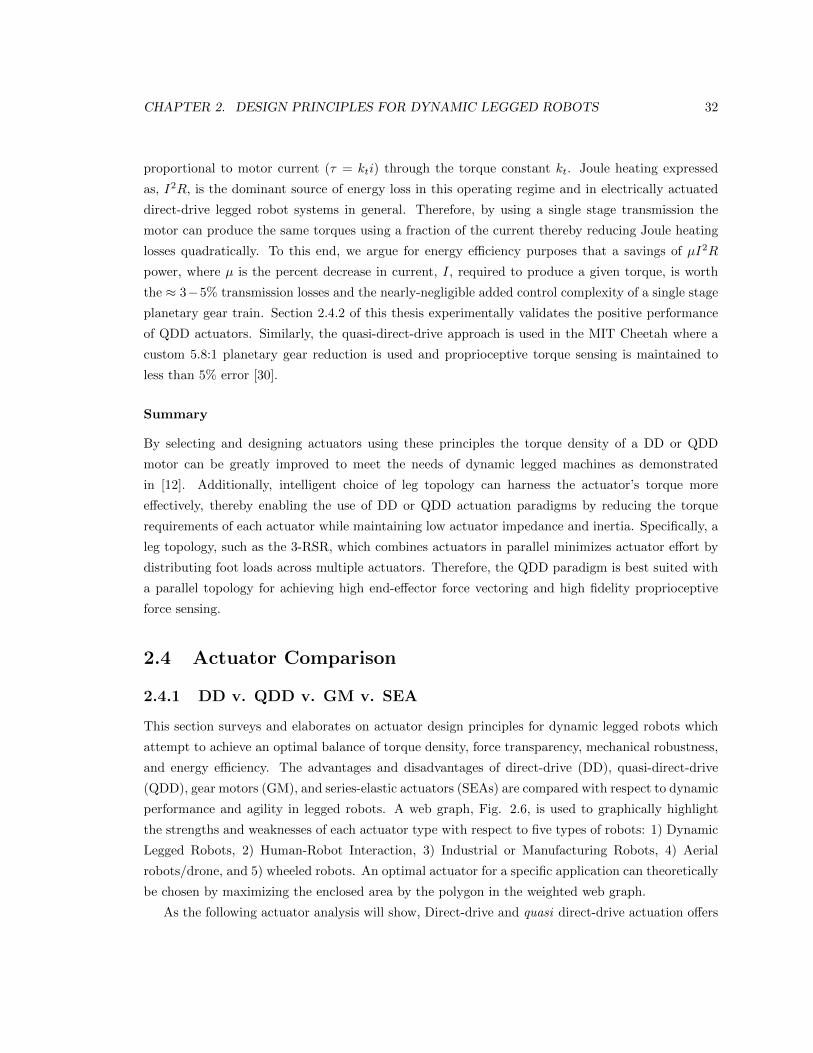
CHAPTER 2. DESIGN PRINCIPLES FOR DYNAMIC LEGGED ROBOTS 32
proportional to motor current (τ = kti) through the torque constant kt. Joule heating expressed
as, I2R, is the dominant source of energy loss in this operating regime and in electrically actuated
direct-drive legged robot systems in general. Therefore, by using a single stage transmission the
motor can produce the same torques using a fraction of the current thereby reducing Joule heating
losses quadratically. To this end, we argue for energy efficiency purposes that a savings of µI2R
power, where µ is the percent decrease in current, I, required to produce a given torque, is worth
the ≈ 3−5% transmission losses and the nearly-negligible added control complexity of a single stage
planetary gear train. Section 2.4.2 of this thesis experimentally validates the positive performance
of QDD actuators. Similarly, the quasi-direct-drive approach is used in the MIT Cheetah where a
custom 5.8:1 planetary gear reduction is used and proprioceptive torque sensing is maintained to
less than 5% error [30].
Summary
By selecting and designing actuators using these principles the torque density of a DD or QDD
motor can be greatly improved to meet the needs of dynamic legged machines as demonstrated
in [12]. Additionally, intelligent choice of leg topology can harness the actuator’s torque more
effectively, thereby enabling the use of DD or QDD actuation paradigms by reducing the torque
requirements of each actuator while maintaining low actuator impedance and inertia. Specifically, a
leg topology, such as the 3-RSR, which combines actuators in parallel minimizes actuator effort by
distributing foot loads across multiple actuators. Therefore, the QDD paradigm is best suited with
a parallel topology for achieving high end-effector force vectoring and high fidelity proprioceptive
force sensing.
2.4 Actuator Comparison
2.4.1 DD v. QDD v. GM v. SEA
This section surveys and elaborates on actuator design principles for dynamic legged robots which
attempt to achieve an optimal balance of torque density, force transparency, mechanical robustness,
and energy efficiency. The advantages and disadvantages of direct-drive (DD), quasi-direct-drive
(QDD), gear motors (GM), and series-elastic actuators (SEAs) are compared with respect to dynamic
performance and agility in legged robots. A web graph, Fig. 2.6, is used to graphically highlight
the strengths and weaknesses of each actuator type with respect to five types of robots: 1) Dynamic
Legged Robots, 2) Human-Robot Interaction, 3) Industrial or Manufacturing Robots, 4) Aerial
robots/drone, and 5) wheeled robots. An optimal actuator for a specific application can theoretically
be chosen by maximizing the enclosed area by the polygon in the weighted web graph.
As the following actuator analysis will show, Direct-drive and quasi direct-drive actuation offers
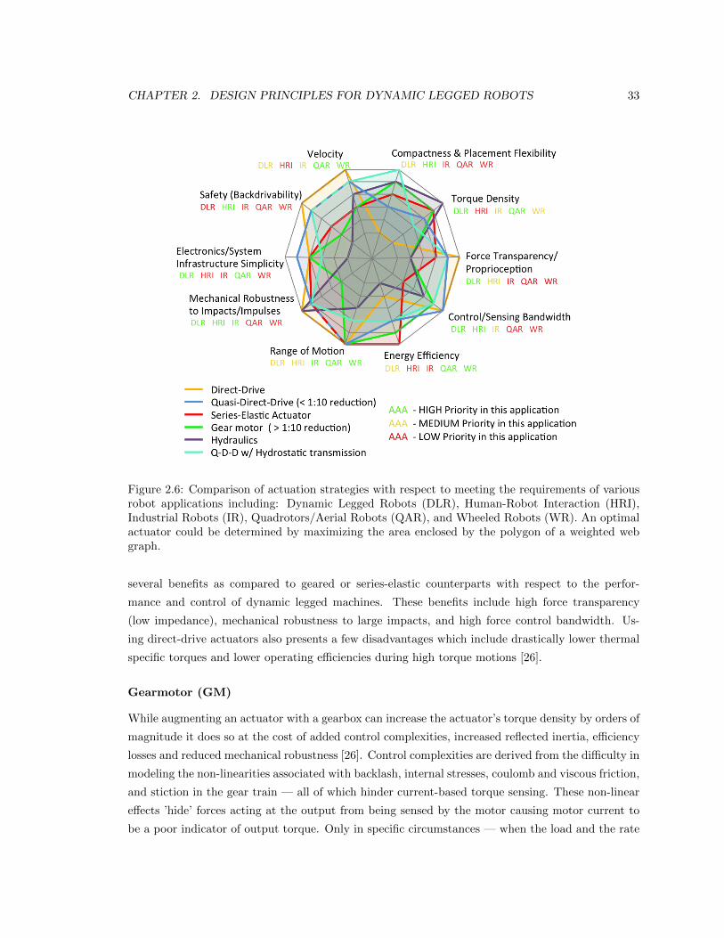
CHAPTER 2. DESIGN PRINCIPLES FOR DYNAMIC LEGGED ROBOTS 33
Figure 2.6: Comparison of actuation strategies with respect to meeting the requirements of variousrobot applications including: Dynamic Legged Robots (DLR), Human-Robot Interaction (HRI),Industrial Robots (IR), Quadrotors/Aerial Robots (QAR), and Wheeled Robots (WR). An optimalactuator could be determined by maximizing the area enclosed by the polygon of a weighted webgraph.
several benefits as compared to geared or series-elastic counterparts with respect to the perfor-
mance and control of dynamic legged machines. These benefits include high force transparency
(low impedance), mechanical robustness to large impacts, and high force control bandwidth. Us-
ing direct-drive actuators also presents a few disadvantages which include drastically lower thermal
specific torques and lower operating efficiencies during high torque motions [26].
Gearmotor (GM)
While augmenting an actuator with a gearbox can increase the actuator’s torque density by orders of
magnitude it does so at the cost of added control complexities, increased reflected inertia, efficiency
losses and reduced mechanical robustness [26]. Control complexities are derived from the difficulty in
modeling the non-linearities associated with backlash, internal stresses, coulomb and viscous friction,
and stiction in the gear train — all of which hinder current-based torque sensing. These non-linear
effects ’hide’ forces acting at the output from being sensed by the motor causing motor current to
be a poor indicator of output torque. Only in specific circumstances — when the load and the rate

CHAPTER 2. DESIGN PRINCIPLES FOR DYNAMIC LEGGED ROBOTS 34
of change of the load are in the same direction, and the output velocity is above a certain threshold
and is not changing sign — was current sensing observed to be a reliable indicator of output torque
on actuators with high gear reductions [55]. The poor motor-current based sensing of gearmotors is
attributed to backlash — which occurs when there is a change in the sign of velocity — and static
friction, which is prevalent when velocity is near zero.
By using higher-end more complex gear trains, backlash can be nearly eliminated and the number
of stages can decrease to one. Harmonic gears offer zero backlash, a lightweight and compact form
factor, and have the greatest torque density per stage but their high reduction ratios introduce large
reflected inertias. Similarly, cycloidal drives offer high gear reduction ratios (high reflected inertia)
in a small form factor with good shock overload capacity but are difficult to manufacture12, suffer
from poor back-drivability (transparency) and lower efficiencies (≈75-85% per stage) due to high
sliding contact [50].
Friction, stiction and reflected inertia in transmissions increase an actuator’s mechanical impedance
and decrease total system bandwidth [17]. In order to track and command faster force trajectories,
the closed-loop bandwidth must be increased by both the actuator and leg design. Therefore, a
high transparency and highly backdrivable actuator — where all force at the output can be sensed
at the input — is optimal for high fidelity and thus high bandwidth proprioceptive force control
[17]. High fidelity proprioceptive force control is desirable for the the control of dynamic legged
machines because it is necessary for effectively producing virtual leg compliance upon impacts and
can be a very high-bandwidth indicator of gait state transitions (i.e. flight to stance phase). The
effect of the transmission ratio n and its corresponding reflected inertia on system bandwidth is
theoretically quantified for a simple 1-DoF actuator shown in Fig. 2.7(b) using equations 2.34-2.35.
In this analysis of actuator bandwidth, ks the series stiffness, can be set to 106 N-m for stiff gear
trains and transmissions without an elastic element.
In addition to the effect gear reductions have on reducing bandwidth, transmissions also undesir-
ably increase inertia. For any mechanical system with a reduction transmission, the effective mass
moment of inertia seen by the input motor for a given output load with inertia Il is derived by a
conservation of energy formulation done in [57]. For a loss-less, ideal gearbox (i.e. negligent internal
gear inertia) at steady-state
τinωin = τoutωout (2.26)
where a reduction gearing would increase torque and decrease speed such that
ωout =1
nωin (2.27)
τout = nτin (2.28)
Solving for the required output torque by Newton’s 2nd law gives
12 manufacturing of cycloidal drivers are difficult due to very tight tolerances required for the cams

CHAPTER 2. DESIGN PRINCIPLES FOR DYNAMIC LEGGED ROBOTS 35
τout = Ilωout (2.29)
Plugging in equations 2.27 and 2.28 into 2.29 the effective inertia becomes
n τin =1
nIlωin (2.30)
τin =1
n2Ilωin (2.31)
Therefore, as seen from the motor input, the load accelerates in response to the input torque as if
the gearbox had been replaced with an output link with a moment of inertia equal to Iln2 [57]. This
increased effective moment of inertia due to the transmission is referred to as reflected inertia and
it scales by n2.
Gears are also inherently prone to being damaged by large impulses which cause tooth shearing.
This is especially true in spur gear trains where the impulse load and impact force is being transferred
over one to two gear teeth as opposed to planetary gears which distribute the load over multiple
planet gears and thus multiple teeth. Because the cross sectional area of a single tooth is very small
the shear stress defined by
τshear =FimpactAc/s
(2.32)
becomes very large for even relatively moderate forces and thus heavy, high strength materials, such
as hardened steel are usually required for high torque applications.
Series Elastic Actuators
In the mid 1990’s Gill Pratt introduced a concept in which a mechanically compliant or ‘elastic’
element was configured in series with the motor shaft and transmission output. He coined this
configuration a Series-Elastic Actuator (SEA) [58]. Since then many robots, both for manipulation
and legged locomotion, have implemented custom SEAs. A few notable robots utilizing SEAs include
StarlETH, ATRIAS, NASA JSC’s Valkyrie [59], Rethink Robotics’ Baxter, and the CMU Biorobotics
SEA-Snake [24].
Series-elastic actuators have been further developed to mitigate negative gear train effects and
regain torque sensing accuracy while maintaining torque density offered by the gear train. SEAs
also offer improved efficiency and mechanical robustness by using elastic energy storage via spring
deflection to passively dampen impulse energy at the actuator’s output from reaching the gear
train or for recycling energy from step-to-step in gaits cycles. However, as a consequence, SEAs
mechanically filter out high frequency dynamics and thus actuation bandwidth is inherently reduced
as shown in Fig. 2.8 by the following analysis described by the model in Fig. 2.7(a).
SEAs employ a variety of spring elements with attempts at maximizing spring linearity, energy
storage, specific energy, passive compliance, or torque sensitivity [24]. Common materials used as

CHAPTER 2. DESIGN PRINCIPLES FOR DYNAMIC LEGGED ROBOTS 36
Im n
ks
bs
τl
τm
gearboxmotor spring
Im n
τl
τm
gearboxmotor
Im
n
τl
τm
gearbox
motor
Im
τl
τm
motor
(a) (b)
(c) (d)
l1
l1
l1
l1
output linkoutput link
output linkoutput link
Figure 2.7: (a) Model of a series elastic actuator with series spring stiffness ks, spring dampeningbs, gear reduction n, and motor rotor inertia Im, (b) is a model of a stiff gear motor, (c) is a modelof a quasi-direct-drive actuator, (d) is a model of a direct-drive actuator. τm and τl are the motorand load torques for a fixed input and output.
the mechanically elastic element include rubber, fiberglass, and steel in torsional. linear, leaf, and
compliant mechanism configurations [24].
A big application of SEAs is in the use of robots that require force control to interact precisely
with the environment and with nearby humans. A big advantageous of SEAs is that they can offer
torque sensing on heavily geared motors that is far more accurate than motor-current based methods.
Torque sensing using SEAs is accomplished with Hooke’s law. This requires using some form of an
encoder to measure spring deflection θ with knowledge of the spring constant ks
τ = ksθ (2.33)
Additional benefits of SEAs are the elastic strain energy storage and delivery capabilities, de-
creased reflected inertia for high reduction transmissions, and inherent shock energy absorption to
protect the the gear train from large impulses.
Energy storage and increased mechanical robustness are perhaps most advantageous for hopping
robots which cyclically store energy in the series-spring upon touch-down impacts and re-deliver it
as thrust energy for take-off in the following cycle. This energy recycling has benefits in energy
efficiency as less input energy is required from the robot’s actuators in each cycle. For example,
ATRIAS stores around 40 J of energy by in each of its 3500 Nm/rad springs during stance of a slow

CHAPTER 2. DESIGN PRINCIPLES FOR DYNAMIC LEGGED ROBOTS 37
Figure 2.8: Impact of spring stiffness on control bandwidth for series elastic actuators.
Figure 2.9: Relationship between actuator inertia and spring stiffness on control bandwidth andimpact force.

CHAPTER 2. DESIGN PRINCIPLES FOR DYNAMIC LEGGED ROBOTS 38
running gait [10]. This corresponds to a 0.15 radian max spring deflection for that particular gait.
Furthermore, smaller power requirements allow actuators to be sized smaller and thus reduce robot
weight and payload.
While SEAs offer stable proprioceptive force sensing, enhanced mechanical robustness and impact
mitigation, passive disturbance rejection, reduced impedance, and compliant position control they
do so at the cost of increased control complexity. The increased complexity arises from the need to
model compliance accurately for inverse dynamics and torque control.
The series-spring is a second order mechanical low-pass filter on high frequency dynamics. Thus,
the spring dampens high frequency impacts upon foot touch-down which can be desirable but it is
also responsible for a reduction in actuation bandwidth which is critical for very dynamic machines
attempting to produce transfer force rapidly. The stiffness of the series-spring determines the maxi-
mum frequencies to which the actuator can command force and position trajectories. Using a simple
SEA model, the theoretical bandwidth can be determined by finding the natural frequency of the
system dynamics. The bandwidth of the actuator is a function of the transmission’s reduction ratio
n, the spring stiffness ks, and the motor’s rotor inertia Im represented by
ωn = B =
√ksn2Im
(2.34)
Similarly, the impact force felt by the actuator is
Fimpact =√
(ks + kg)n2Im (2.35)
where kg is the effective stiffness of the contact point in the environment [17].
Direct-Drive and Quasi-Direct-Drive
Using a larger direct-drive actuator to achieve a required torque without gear reduction increases
the volume and weight of the actuator as compared to geared counterparts but it preserves the high
transparency and low impedance that are crucial to high bandwidth proprioceptive force control.
Additionally, the mechanical robustness and structural integrity of direct-drive systems are higher
as compared to geared systems because there are fewer components to protect from large impulses
ubiquitous in running, jumping and landing behaviors [26][12].
For a direct-drive system, the impulse forces at the foot are transmitted to the body through the
leg Jacobian directly through the motors air gap [12]. This minimizes components in the load path
that are susceptible to failure making for a more robust and resilient machine.
Should a transmission stage be used to achieve the required application torque I argue and show
in the following analysis and experimental actuator comparison that an ideal actuator configuration
for high speed running and jumping robots when considering efficiency is a single-stage planetary
gear train with a reduction of at most 1:10. Single-stage planetary gears with reductions greater
than 1:10 are not possible because pinion (sun) gears can only be made so small and as the reduction

CHAPTER 2. DESIGN PRINCIPLES FOR DYNAMIC LEGGED ROBOTS 39
Ring Gear: Fixed
Planet Carrier: Output Planet Gears
Sun Gear: Input
Figure 2.10: The ideal configuration for maximizing reduction of a single-stage planetary gear isto fix the ring gear, couple the sun gear to the motor input, and the planet carrier to the output.Circles represent the gear’s pitch radius so teeth are not shown.
ratio increases for a given ring size the sun gear pitch radius decreases and the planet gear pitch radii
increase [60]. This leads to a design trade-off in which high reduction ratios produce higher torque
outputs but as higher ratios are designed less planet gears can geometrically fit without interference,
meaning impulse loads are distributed over less planet gears (and less individual gear teeth) which
decreases overall resiliency/robustness of the gear-train. Planetaries with lower reduction ratios can
have 4 to 5 planet gears for improved load rating while higher reductions of 1:10 can only have 2
planet gears. Other gear trains such as a harmonic and cycloidal drives, with a typical reduction of
1:100, will have reflected joint inertias ( IN2 ) that approach the inertia of the robot’s mass [21]. I refer
to this actuator design as quasi -direct-drive (QDD) for its proximity to properties of true direct-
drive systems. Quasi-direct-drive actuators preserve force transparency for accurate proprioceptive
sensing while offering torque magnification for only marginal sacrifices in added impedance, reflected
inertia and mechanical robustness. Planetary gears are compact, low profile, low weight, low cost,
backdrivable, distribute loads over multiple planet gears (30-50% greater load capacity than spur
gears), have minimal backlash (typically less than 13 arc-min or 0.21o), and high efficiencies (≈95-97% per stage), while offering reduction ratios up to 10:1 for a single stage.
2.4.2 Experimental Validation of Actuator Properties
To experimentally verify the results of the theoretical analysis and comparison of DD, QDD, GM,
and SEA actuators a series of experiments was conducted. The experimental force bandwidth, rise
time, settling time, peak time, overshoot, and proprioceptive torque sensing accuracy and error are

CHAPTER 2. DESIGN PRINCIPLES FOR DYNAMIC LEGGED ROBOTS 40
(a) (b) (c) (d)
Figure 2.11: Actuators configured as (a) Direct drive, (b) quasi-direct-drive (1-stage planetary), (c)gear motor (2-stage planetary), and (d) Hebi X-5 SEA module in the torque testing rig. The motorback is fixed directly to a mounting plate and the output of the actuator is coupled to the 1-axisload cell whose housing is also bolted to the rig.
calculated and shown by the following plots in Fig. 2.12-2.16.
Fig. 2.11 shows the test rig used to conduct all the experiments whose results are shown in Table
2.4.2. The DD actuator is a T-motor U10 with no transmission. Single planetary gear stages were
added to the direct-drive T-motor to test QDD (1 added stage) and GM (2 added stages). Each
added gear stage is a COTS Matex 75-7MLD (7:1) planetary gear. Rather than arduously designing
a custom SEA for the sole purpose of this testing, an available COTS SEA (Hebi X5-1 module) was
chosen to match the continuous torque rating of the DD actuator. Therefore, For DD, QDD, and
GM a T-motor U10 was the driving motor, while a much smaller Maxon EC-Max 16, 5W motor
with a 272:1 gear reduction was used in the SEA. The different motor’s have an effect on system
inertia but the bandwidth trends validated in this test hold true regardless of the fact that different
motors were used. All tests on all four actuators were done on the same test rig using a single axis
SRI M2210E torque load cell.
Bandwidth
Each of the actuators was tested by commanding sinusoidal torque trajectories of increasing fre-
quency until the actuator could no longer following the trajectory with adequate accuracy. The
sinusoidal torque frequencies ranged from 1 Hz to the 100 Hz. The following bandwidth plots for
each actuator show (a) a stable frequency, (c) max frequency with adequate trajectory following
or actuator bandwidth, and (b) a frequency in between. For reference and comparison purposes,
the MIT Cheetah (QDD), HyQ (hydraulic), and StarlETH (SEA) actuators have maximum force
control bandwidths of 103 Hz [9], 15-20 Hz [8], 11-28 Hz, and [11]. Humans and animals on the other
hand have a control bandwidth of only 4-8 Hz which implies that the majority of the dynamics in

CHAPTER 2. DESIGN PRINCIPLES FOR DYNAMIC LEGGED ROBOTS 41
running and jumping occur passively in muscles and tendons [21].
The direct drive actuator in Fig. 2.12 shows frequencies of 20, 70 and 100 Hz. The DD actuator
was capable of following torque trajectories with an amplitude of 1.5 N-m accurately up to 70
Hz although at 70 Hz there is nearly a 1800 phase while the torque amplitude remains accurate.
The direct drive actuator demonstrated a bandwidth of up to 250 Hz for small, same-sign, torque
variations on the order of 0.1 to 0.5 N-m in Fig. 4.6. The quasi-direct-drive actuator in Fig. 2.13
shows response at 20, 30, and 40 Hz. A phase offset close to 1800 can be seen at 20 Hz but the
actuator is still able to exert torque at commanded amplitude at 20 Hz and higher frequencies without
significant loss of fidelity in torque profile or shape response. The maximum achievable frequency
with adequate trajectory following for the QDD was determined to be 40 Hz, therefore this is the
systems force bandwidth. The gear motor in Fig. 2.14 shows tests of 10, 20, and 40 Hz. While the
trajectory amplitude is not followed very closely the frequency is maintained up to nearly 40 Hz.
However, 40 Hz should not be considered as the system bandwidth because the torque amplitude has
significant error over 100%. This can be due to the gear-trains relatively large backlash attenuating
over 2 stages. The backlash was significant enough such that the motor could actually spin ±360o
when coupled to the load cell which would not allow for any motion if the actuator had zero backlash.
Comparatively, in the QDD actuator the input motor rotor was able to rotate about ±45o which
is also relatively significant. The DD actuator was not able to rotate at all which makes sense as
there is zero backlash as the rotor is directly bolted to the load cell without any transmission where
backlash can accrue. Therefore, the system bandwidth for this particular gear motor (GM) actuator
is approximated at around 25-30 Hz. The final actuator tested was the series elastic actuator which
is a Hebi Robotics X5-1 module which uses a series-spring with 70Nm/rad stiffness, a 272:1 spur
gear reduction over 3 stages and is manufacturer rated at 0.25o of backlash. Fig. 2.15 shows that
the Hebi X5-1 module is rather accurate in tracking torque trajectories by measuring the spring
deformation of their natural rubber series-springs. The response begins to diminish in amplitude
tracking at around 25 Hz and reaches a phase offset of 180o at 30 Hz. Therefore, the experimentally
determined bandwidth of the system is approximated at 25-30Hz.
Thus, it is clear that direct-drive is far superior nearly doubling the bandwidth of the alterna-
tive actuator configurations. However, since a stock, COTS, Matex planetary gear is used with a
significant 1.2o rated backlash, the bandwidth can reasonably be expected to be lower than that of
an actuator using a custom, application-optimized, planetary gear designed to minimize backlash,
maximize load rating, and minimize weight as done in [9]. Since budget was a factor in these exper-
iments these cheap $75 gear trains were sufficient to understanding the general influence gear trains
had on actuator bandwidth.
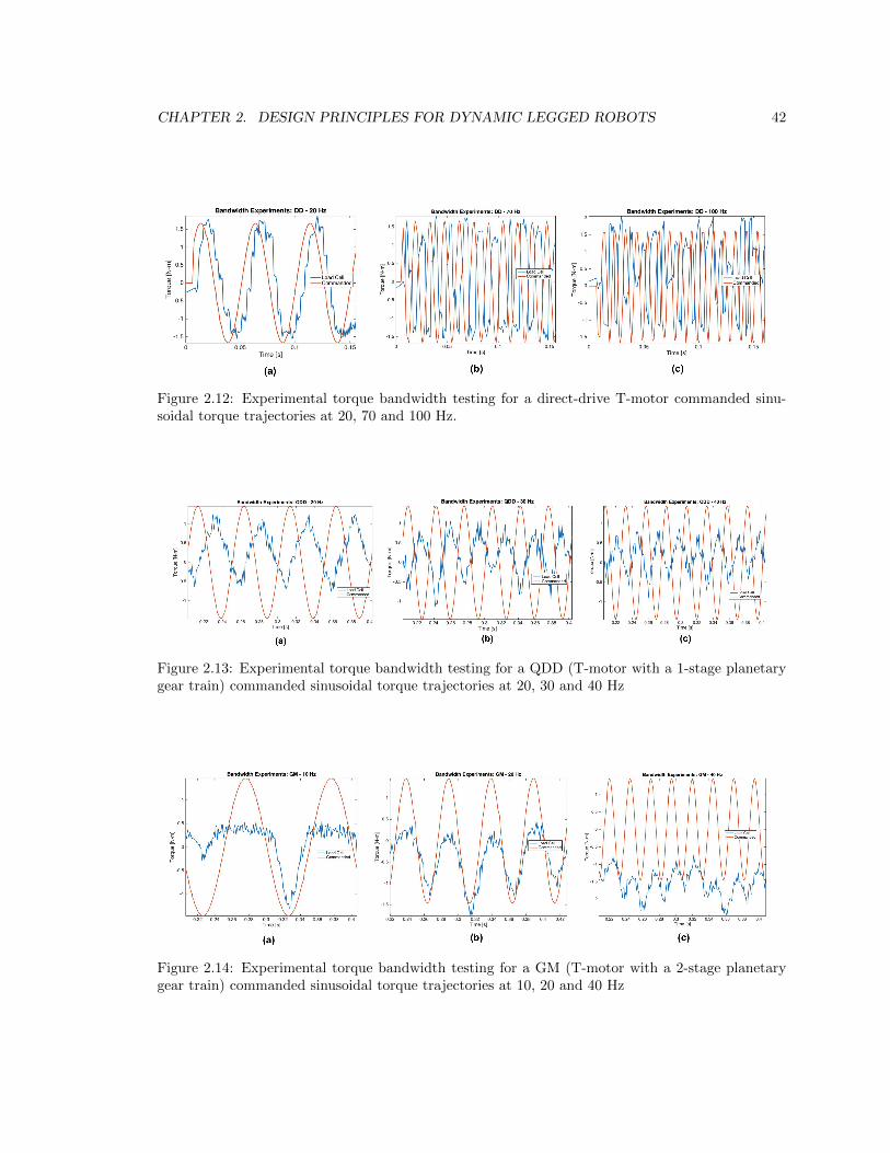
CHAPTER 2. DESIGN PRINCIPLES FOR DYNAMIC LEGGED ROBOTS 42
Figure 2.12: Experimental torque bandwidth testing for a direct-drive T-motor commanded sinu-soidal torque trajectories at 20, 70 and 100 Hz.
Figure 2.13: Experimental torque bandwidth testing for a QDD (T-motor with a 1-stage planetarygear train) commanded sinusoidal torque trajectories at 20, 30 and 40 Hz
Figure 2.14: Experimental torque bandwidth testing for a GM (T-motor with a 2-stage planetarygear train) commanded sinusoidal torque trajectories at 10, 20 and 40 Hz

CHAPTER 2. DESIGN PRINCIPLES FOR DYNAMIC LEGGED ROBOTS 43
Figure 2.15: Experimental torque bandwidth testing for a SEA (Hebi X5-1) commanded sinusoidaltorque trajectories at 10, 20 and 30 Hz.
Proprioceptive Torque Sensing and Rise Time
Because proprioceptive sensing is also of utmost importance in addition to sufficient actuator band-
width a series of tests were done to measure proprioceptive torque sensing and control accuracy in
addition to other traditional actuator performance metrics such as rise time, settling time, overshoot,
etc. These results for the 4 actuator types are shown in Fig. 2.16 and the measured performance
metrics are all summarized in Table 2.4.2. Fig. 2.16 indicates that DD and QDD actuators have
very accurate proprioceptive torque control and sensing to within 0.05 and 0.4 N-m accuracy which
corresponds to 12 and 5.4 percent error, respectively. Proprioceptive sensing for GM and SEA con-
figurations are less ideal where errors reach 24 and 28 percent, respectively. It is important to also
note that rise time — an important metric for measuring how fast an actuator can generate torque
from rest or change torque in a step response — from DD to QDD only differs by 5.8 ms. However,
by adding just one more planetary gear stage to the QDD to get the 2-stage GM configuration the
rise time differs by a much larger 116.9 ms. Therefore, the advantages of direct-drive are for the most
part proven to be preserved by the addition of only a single stage planetary gear stage. Additionally,
with the use of a custom designed single stage gear train or a higher-end COTS planetary gear the
performance of QDD can be expected to increase and further converge on the desirable performance
of the direct-drive approach.
Table 2.4.2 summarizes the series of experiments conducted on the four discussed actuator types:
DD, QDD, GM, and SEA. The quantitative results match expected theoretical analysis and relative
performance as compared to one another. With a priority on achieving high agility and virtual
compliance the specifications of most interest again are accurate, high bandwidth torque sensing
and actuation and high force/speed while considering energy efficiency and mechanical robustness
factors. Therefore, in this regard and with the mentioned priorities the QDD actuator seems to be
the ideal actuator for the particular application of dynamic legged robots.

CHAPTER 2. DESIGN PRINCIPLES FOR DYNAMIC LEGGED ROBOTS 44
(a) (b)
(c) (d)
Figure 2.16: (a) DD, (b) QDD, (c) GM, (d) SEA. Rise time, settling time, peak time, overshoot, andproprioceptive torque sensing accuracy and error are calculated using the following step responseexperiments shown here.
Summary
There are countless design trade-offs and competing design goals when considering actuator design
and synthesis of leg topologies to achieve desired performance. It is important to choose a leg
topology and actuation scheme which compliment one another to achieve the design specifications
for maximum dynamic legged mobility! The following flow charts in Fig. 2.17 and 2.18 show the
design methodology and trade-offs for each type of actuator and the resulting robots (or examples
of robots) that are produced. The design methodology starts with an unmodified electric brushless
DC motor where torque is the limiting resource. Hydraulics, electro-hydraulics, and pneumatics
were ruled out of consideration in this thesis because of the large overhead infrastructure (heat
exchangers, pumps, internal combustion engines, hydraulic pressure units, etc.), inefficiency (mainly
hydraulics), and high impedance of these actuator types.

CHAPTER 2. DESIGN PRINCIPLES FOR DYNAMIC LEGGED ROBOTS 45
Figure 2.17: Methodology for actuator selection and design starting from the basic, unmodifiedelectric motor where torque is the limiting resource. This specific methodology flow results in robotslike StarlETH [11], ATRIAS [10], and BiMASC [21].
Figure 2.18: Methodology for actuator selection and design starting from the basic, unmodifiedelectric motor where torque is the limiting resource. This specific methodology flow results in robotslike MIT Cheetah [9], Penn Minitaur [12], and GOAT, the robot introduced in this thesis.
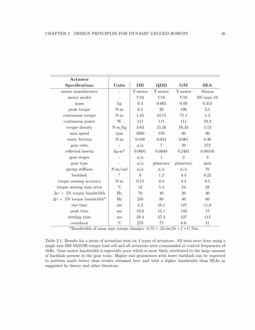
CHAPTER 2. DESIGN PRINCIPLES FOR DYNAMIC LEGGED ROBOTS 46
Actuator
Specifications Units DD QDD GM SEA
motor manufacturer - T-motor T-motor T-motor Maxon
motor model - U10 U10 U10 EC-max 16
mass kg 0.4 0.665 0.93 0.315
peak torque N-m 6.5 28 196 2.5
continuous torque N-m 1.45 10.15 71.1 1.3
continuous power W 111 111 111 19.2
torque density N-m/kg 3.63 15.26 76.34 4.13
max speed rpm 4000 570 80 90
static friction N-m 0.048 0.054 0.061 0.36
gear ratio - n/a 7 49 272
reflected inertia kg-m2 0.0001 0.0049 0.2401 0.00316
gear stages - n/a 1 2 3
gear type - n/a planetary planetary spur
spring stiffness N-m/rad n/a n/a n/a 70
backlash o 0 1.2 8.4 0.25
torque sensing accuracy N-m 0.15 0.4 4.4 0.5
torque sensing max error % 12 5.4 24 28
∆τ > .5N torque bandwidth Hz 70 40 20 30
∆τ < .5N torque bandwidth* Hz 250 90 40 60
rise time ms 4.3 10.1 127 11.0
peak time ms 10.0 15.1 133 17
settling time ms 33.4 37.3 137 113
overshoot % 273 77 6.6 51
*Bandwidth of same sign torque changes: 0.75 + .25 sin(2π ∗ f ∗ t) Nm.
Table 2.1: Results for a series of actuation tests on 4 types of actuators. All tests were done using asingle axis SRI M2210E torque load cell and all actuators were commanded at control frequencies of1kHz. Gear motor bandwidth is especially poor which is most likely attributed to the large amountof backlash present in the gear train. Higher end gearmotors with lower backlash can be expectedto perform much better than results obtained here and with a higher bandwidth than SEAs assuggested by theory and other literature.
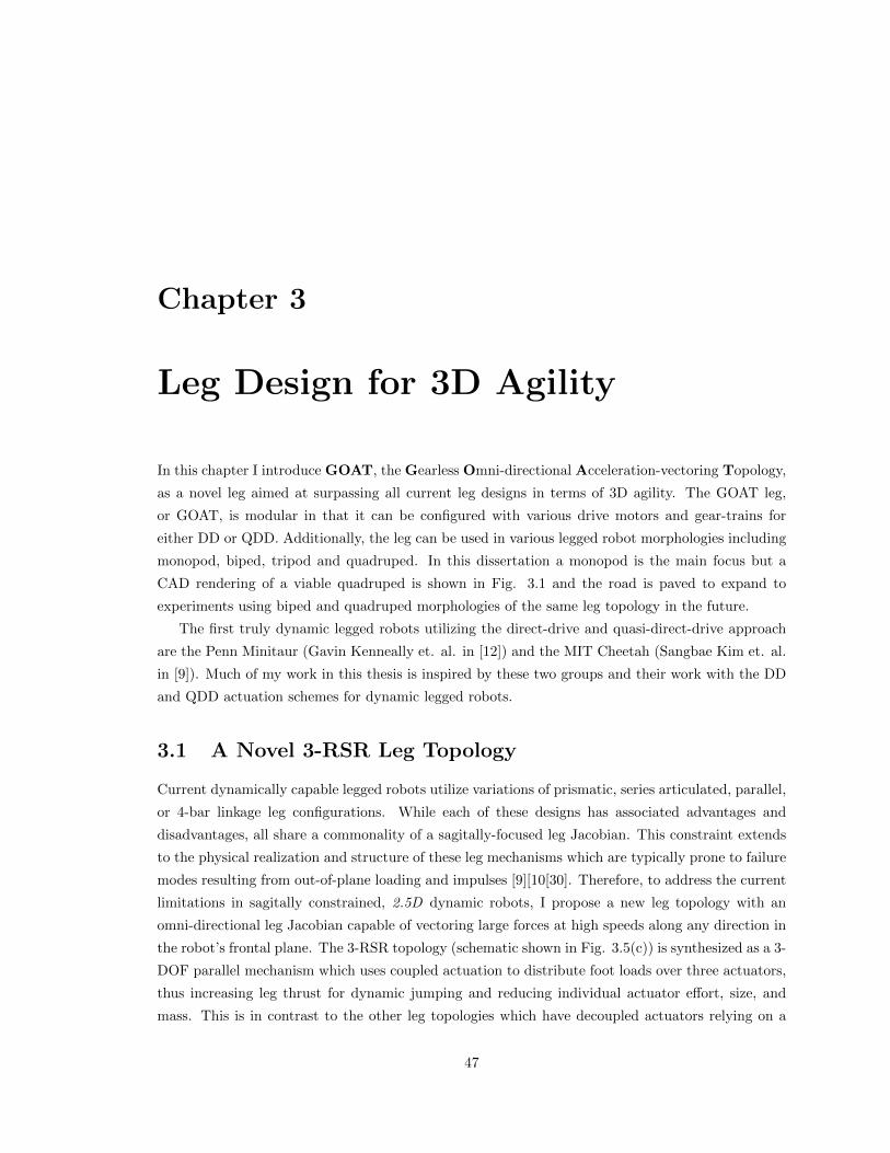
Chapter 3
Leg Design for 3D Agility
In this chapter I introduce GOAT, the Gearless Omni-directional Acceleration-vectoring Topology,
as a novel leg aimed at surpassing all current leg designs in terms of 3D agility. The GOAT leg,
or GOAT, is modular in that it can be configured with various drive motors and gear-trains for
either DD or QDD. Additionally, the leg can be used in various legged robot morphologies including
monopod, biped, tripod and quadruped. In this dissertation a monopod is the main focus but a
CAD rendering of a viable quadruped is shown in Fig. 3.1 and the road is paved to expand to
experiments using biped and quadruped morphologies of the same leg topology in the future.
The first truly dynamic legged robots utilizing the direct-drive and quasi-direct-drive approach
are the Penn Minitaur (Gavin Kenneally et. al. in [12]) and the MIT Cheetah (Sangbae Kim et. al.
in [9]). Much of my work in this thesis is inspired by these two groups and their work with the DD
and QDD actuation schemes for dynamic legged robots.
3.1 A Novel 3-RSR Leg Topology
Current dynamically capable legged robots utilize variations of prismatic, series articulated, parallel,
or 4-bar linkage leg configurations. While each of these designs has associated advantages and
disadvantages, all share a commonality of a sagitally-focused leg Jacobian. This constraint extends
to the physical realization and structure of these leg mechanisms which are typically prone to failure
modes resulting from out-of-plane loading and impulses [9][10[30]. Therefore, to address the current
limitations in sagitally constrained, 2.5D dynamic robots, I propose a new leg topology with an
omni-directional leg Jacobian capable of vectoring large forces at high speeds along any direction in
the robot’s frontal plane. The 3-RSR topology (schematic shown in Fig. 3.5(c)) is synthesized as a 3-
DOF parallel mechanism which uses coupled actuation to distribute foot loads over three actuators,
thus increasing leg thrust for dynamic jumping and reducing individual actuator effort, size, and
mass. This is in contrast to the other leg topologies which have decoupled actuators relying on a
47

CHAPTER 3. LEG DESIGN FOR 3D AGILITY 48
Figure 3.1: CAD Rendering of a viable quadruped using the GOAT leg topology.
single actuator for producing sagittal plane thrust forces and another actuator for producing dorsal
plane forces. I describe the kinematics of the 3-DOF, 3-RSR parallel linkage and follow up with
an optimization of the mechanism parameters to maximize omni-directional workspace and force
map/envelope. Finally, I detail the mechanical design and physical realization of the mechanism.
3.1.1 Kinematics
Forward and Inverse Kinematics
It is well known that the forward kinematics for spatial parallel linkages can be difficult and some-
times impossible to solve analytically. Therefore, to avoid the complexity in determining a closed
form solution, the 3-RSR’s forward and inverse kinematics are solved using MATLAB’s lsqnonlin()
function and mexxed to C++ for real time constrained optimization. Nine constraint equations
construct the cost function for the forward and inverse kinematics optimization. A binary term in
the cost function constrains the z-component of foot plate normal to be negative. For the forward
kinematics each knee position ki is known as a function of θ, the actuated joint R1 at the hip from
Fig. 3.2. The constraint eqs. used to solved the kinematics are
0 = w1
((ax,i − kx,i)2 + (ay,i − ky,i)2 + (az,i − kz,i)2 − l22
)(3.1)
0 = w2
((ax,i − ax,i+1)2 + (ay,i − ay,i+1)2 + (az,i − az,i+1)2 − f2
)(3.2)
0 = w3
(nb · nk,i
)(3.3)

CHAPTER 3. LEG DESIGN FOR 3D AGILITY 49
(a) (b) (c)
a1 a3
a2
k1 k2 k3
P
R1
R2
R3
R4 R5
Figure 3.2: the 3-RSR leg topology decomposed into the individual joints at the hip R1, kneeR2,R3,R4, and ankle R5. Although the mechanism is a 3-RSR the physical realization of the topologyis achieved using a 3-RRRRR where the three knee R-joints intersect at a single point for an effectivemobility equal to that of a spherical joint.
where,
nb =(a1 − a2)× (a2 − a3)
||(a1 − a2)× (a2 − a3)||
nk,i =(ki − ai)× (ai −P)
||(ki − ai)× (ai −P)||where, i = 1, 2, 3 represents each chain of the 3-RSR, wi is the weight for each constraint in the cost
function, P is the [x, y, z]T position of the foot center, ai is the [x, y, z]T position of each chain’s
‘ankle’ revolute (R-joint), f is the fixed perpendicular distance between each ankle R-joint, and ki
represents the [x, y, z]T position of each chain’s spherical ‘knee’ joint calculated by
ki = hi ∗Th2k = [RR1(θi), l1]
In Fig. 3.5c The ‘ankle’ joints are the 3 R-joints (denoted R5) at the distal foot plate, the ‘knee’
joints is the point where R2, R3, and R4 intersect, and the hip joints are attached the top hip plate
and denoted by R1. The first set of 3 constraint equations (eq. 3.1) constrains the distance between
the the knee and corresponding ankle joints to be equal to the length of link 1 (l2). The second set
of constraint equations (eq. 3.2) constrains the distance between adjacent ankle joints to be equal
to f . The third set of constraints (eq. 3.3) forces each of the 3 link 2s (l2) in the 3-RSR to be
orthogonal to the foot plate normal because the ankle joint is a 1-DoF revolute joint.
The MEXed MATLAB code compiles and executes the constraint equations in C through each
iteration in the MATLAB optimization. Real-time optimization can be achieved at 100 Hz using
this method. However, to achieve high fidelity virtual compliance (which is the ultimate goal) the

CHAPTER 3. LEG DESIGN FOR 3D AGILITY 50
Figure 3.3: Optimization of link 1 length, l1, for maximum workspace and force production basedon the objective function in eq. 3.5. Here the objective function is scaled to fit the left y-axis.
required control frequency must be close to 1 kHz. Thus, a look-up table for the forward and inverse
kinematics is created to meet the control frequency operating constraint. Using the look-up table,
and a MEXed look-up search function, solutions to the kinematics can be obtained at greater than
1 kHz rate.
The 3-RSR form factor and workspace appear similar to that of a Delta robot arm which is a
purely translational 3-DoF mechanism (unlike the 3-RSR). By removing the parallelism (translation
only) constraint, advantageous for rapid pick-and-place operations, the kinematic workspace of the
end-effector is increased and the mechanism becomes lighter and structurally more robust1 Tradi-
tional Delta Arms have a limited payload and thus are not structurally robust in withstanding or
delivering large environmental forces. Additionally, the Delta robot utilizes a 4-bar linkage as its
second link which adds complexity, parts, inertia, and failure modes.
Jacobian
Because the primary control mode for this leg will be force control employing virtual model control
through the use of virtual spring and damper components the Jacobian — which is a transforma-
tion of infinitesimal kinematics between joint velocity/torques to end-effector velocity/force-torque-
wrench — is needed. Like the forward and inverse kinematics the Jacobian is solved numerically by
differentiating the forward kinematics transformation matrix with ε = 10−6 for adequate numerical
1The Delta Robot arm is kinematically equivalent to a 3-RUU but uses 3 parallel planar 4-bar linkages to connectthe ‘knee’ joints to the ‘foot’ plate or end-effector. The parallel 4-bar constrains the top and bottom plates to beparallel but adds design complexity, weight, and inertia to distal portions of the leg.

CHAPTER 3. LEG DESIGN FOR 3D AGILITY 51
accuracy. For the 3-RSR leg, the Jacobian is a 6 by 3 matrix2 where each column in the matrix
describes each of the 3 actuators contribution to the 6-axis force-torque wrench at the end-effector
(i.e. foot). The Jacobian is constructed as follows
J6×3(θ) =
[T3×3
Ω3×3
](3.4)
T3×3 =1
ε
[bt,1 − at,1,bt,2 − at,2,bt,3 − at,3
]Ω3×3 =
AR,i
2ε
[W32 −W23,W13 −W31,W21 −W12
]T
where W = ATRBR and Bi = Th2f (θ + ε) = [BR,i,bt,i], Ai = Th2f (θ) = [AR,i,at,i] are transfor-
mations from the hip to the foot Th2f , for chain i, with input hip angles θ + ε and θ, respectively.
Parameter Optimization
To maximize workspace and average force production throughout the workspace an optimization,
shown in Fig. 3.3, was conducted to determine the leg link lengths, l1 and l2, and hip/foot radii, rh
and rf respectively, over a range of physically tractable dimensions. The optimization maximized
the following objective function O over the parameters: q = [l1, l2, rh, rf ]
O(q) =(c1(q) ∗ c2(q)
)·(c1(q) + c2(q)
)(3.5)
where, c1 = w1 ∗ Vws is the normalized volume of the mechanism’s workspace and c2 = w2 ∗ Favg is
the mean force produced throughout the usable workspace. This optimization yields link lengths of
l1 = 0.165, l2 = .3, rh = .05, and rf = .01, where rh and rf are the respective radii from the hip
and foot plate center to R-joints R1 and R5 from Fig. 3.5(c). This optimization yields a kinematic
workspace with two leg configurations (knee-above-the-hip and knee-below-the-hip shown in Fig.
3.30) where the transition between configurations does not pass through a singularity similar to the
simpler 2-DoF planar parallel Minitaur leg [12]. Having both configurations available nearly doubles
the usable workspace of the limb to a volume of 0.0285m3 as compared to traditional parallel linkages
which only use knee-below-hip configuration in which case the workspace volume with identical leg
parameters would be 0.0151m3. Using the entire workspace allows the leg to deliver 1.68 times more
kinetic energy to the body while decreasing energy losses due to landing collisions, as seen in Fig.
3.30. The kinetic energy delivered to the body is calculated by
E =
∫ θf
θ0
(F (τ, θ) · d(θ) cos(φ)
)dθ (3.6)
2the size of the Jacobian is 6 by 3 because the force-torque wrench is a 6x1 vector and the number of drivenactuators is 3 or a 1x3 vector.

CHAPTER 3. LEG DESIGN FOR 3D AGILITY 52
Figure 3.4: Characterization of the joint torques, foot position, foot velocity, and foot force for avertical jump. The foot force plot shows force produced by constant hip joint torques of 5 N-m foran example vertical foot trajectory where all 3 hip angles are the same due to symmetry. The jointtorque plot shows the actuator torques required to produce a constant 100N for downwards at thefoot. For a vertical leg trajectory all 3 joint angles are the same for each point in the trajectorysince the mechanism is symmetric. For omni-direcitonal force vectoring the joint angles and torqueswill not be the same.
where θ0 = 0o for the full workspace while θ0 = 90o for traditional knee-below-hip only configuration.
F is the foot force, d is the traveled foot distance, and φ is the angle between F and d. θf = 180o
for both configurations. The mechanical realization of the 3-RSR linkage has a slightly smaller
input angle range due to physical interference constraints (30-150o as opposed to 0-180o). With the
physically tractable joint ranges this linkage is capable of transferring 27.0 J of energy to the body
per jump per leg whereas the traditional knee-below-hip design only delivers 19.1 J of energy to the
body.
Additionally, the inherent symmetry of the leg enables omni-directional force and body-acceleration
vectoring. Because the actuators for leg motion in the sagittal and dorsal planes are directly coupled,
the leg distributes foot loads over all 3 actuators to produce foot forces in the sagittal plane, dorsal
plane, or a force vector with components in both the sagittal and dorsal planes (i.e. any vector in
the frontal plane)3.
Fig. 3.4 characterizes the kinematic relationship between the applied hip-joint torques, foot
forces, foot position and velocity for an example vertical foot trajectory. Using the transpose of
3SE(n) refers to the Special Euclidean group where degrees of freedom for SE(n) is n(n + 1)/2, which gives 3(x, y, θ) when n = 2, and 6 (x, y, z, α, β, γ) when n = 3.

CHAPTER 3. LEG DESIGN FOR 3D AGILITY 53
(a) (b) (c)
Figure 3.5: Kinematic diagrams showing leg parameters (Table 3.1 and joint axes for (a) 3-DoFprismatic, (b) 3-DoF series-articulated, and (c) 3-DoF 3-RSR Parallel Spatial topologies.
the leg Jacobian, the joint torques required to produce a force-torque wrench at the foot with a
z-component of −100N can be calculated. Similarly, the entire omni-directional force envelope is
quantitatively determined and plotted in Figs. 3.6 and 3.7. The relatively large workspace and
force envelope of this mechanism, as compared to traditional parallel linkages, shows potential
for enhanced jumping by utilizing the two regions of maximum force production — located at the
proximal and distal regions of the workspace — and high foot speeds in the middle of the workspace.
3.2 Comparison of 3-DoF Leg Topologies
Here I show that the 3-RSR leg topology is advantageous over other, more common, leg topologies
for proprioceptive sensing and explosive omni-directional jumping maneuvers (i.e. 3D agility). In
Figs. 3.6, 3.7, and 3.8 and Table 3.2 I compare the 3-RSR leg against conventional series-articulated
leg designs (MIT Cheetah, StarlETH, SpotMini) and prismatic legs (Raibert Hopper, simplified
SCHAFT 2016) in end-effector workspace and force envelope.
I define four measures of legged 3D agility listed in Table 3.2 as the energy delivered by leg thrust
(E); the force envelope volume (Ψ) which describes how much force can be exerted over the limb’s
workspace; the foot force to leg mass ratio, or limb acceleration (Λ); and the proprioceptive force
sensitivity (Π) which is a metric of the minimal joint torque resolution required to measure a change
in foot force f to f + ε at foot position i within the limbs workspace, where ε is arbitrarily small (1
N in this study). These measures are normalized by assuming all leg topologies have an identical
set of 3 equally sized and performing actuators.

CHAPTER 3. LEG DESIGN FOR 3D AGILITY 54
E = Favg
(dfoot
)max
(3.7)
Ψ = Favg · Vws (3.8)
Λ =Favgml
(3.9)
Π =1
n
n∑i=1
|JTi F (f)− JTi F (f + ε)| (3.10)
where Favg is the average foot force along a foot trajectory, ml is the unsprung leg mass, and
(dfoot)max is the maximum distance traveled by the foot along a linearly extending trajectory as
shown by example in Fig. 3.7(c) by the black line. (dfoot)max is a function of the limbs workspace
Vws.
TopologyLeg Parameters
[kg] [m, m, m] [deg, deg, deg]
ml l0 l1 l2 J1 J2 J3
Prismatic .91 n/a .254 n/a 360 56 .25m
Series .46 .05 .225 .225 40 150 107
3-RSR .63 .05* .165 .3 120 120 120
Refer to Fig. 3.5 for parameter definitions. Parameters for prismatic & series articulated topologies aretaken from the Raibert Hopper & MIT Cheetah legs [6][38].
Note:* Indicates dimension of the 3-RSR’s hip radius which is not a moving link.
Table 3.1: Comparison of leg parameters for three different 3-DoF leg topologies.
3.2.1 Force Envelope Analysis
Figures 3.7, 3.6 show that to produce a force-torque wrench, Ffoot, as defined in eq. 3.12 the required
joint torques are smaller for the 3-RSR leg than for the other topologies. The plots are generated
using a quasi-static force analysis in which joint torques are solved using the Jacobian transpose
method
τm = JTFfoot (3.11)
Ffoot = f [− sinφ sin θ,− sinφ cos θ, cosφ, 0, 0, 0]T (3.12)
where f = −100 N, φ = tan−1( step lengthstep height ), and θ is the direction or heading in the frontal plane
(θ = 0o points in direction of +Y).
The 3-RSR parallel leg topology shows advantages over series-articulated legs by allowing all
actuators to be placed in the hip/body maintaining a very low inertia, and thus high speed, limb.
The MIT cheetah minimizes this effect in its serial-articulated limb by locating the hip and knee
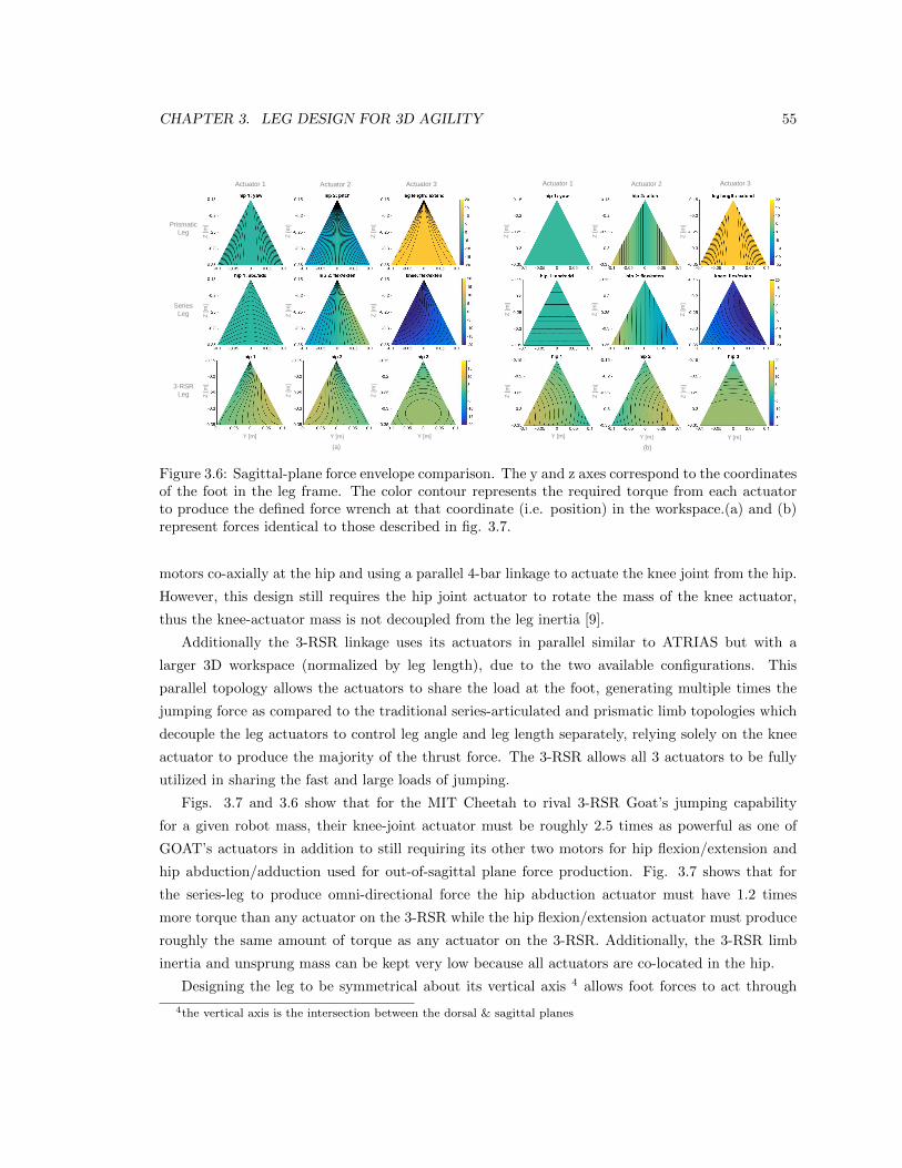
CHAPTER 3. LEG DESIGN FOR 3D AGILITY 55
Actuator 1 Actuator 2 Actuator 3
Series Leg
Prismatic Leg
3-RSR Leg
Actuator 1 Actuator 2 Actuator 3
(a) (b)
Y [m] Y [m] Y [m] Y [m] Y [m] Y [m]
Z [m
] Z
[m]
Z [m
]
Z [m
] Z
[m]
Z [m
]
Z [m
] Z
[m]
Z [m
]
Z [m
] Z
[m]
Z [m
]
Z [m
] Z
[m]
Z [m
]
Z [m
] Z
[m]
Z [m
]
Figure 3.6: Sagittal-plane force envelope comparison. The y and z axes correspond to the coordinatesof the foot in the leg frame. The color contour represents the required torque from each actuatorto produce the defined force wrench at that coordinate (i.e. position) in the workspace.(a) and (b)represent forces identical to those described in fig. 3.7.
motors co-axially at the hip and using a parallel 4-bar linkage to actuate the knee joint from the hip.
However, this design still requires the hip joint actuator to rotate the mass of the knee actuator,
thus the knee-actuator mass is not decoupled from the leg inertia [9].
Additionally the 3-RSR linkage uses its actuators in parallel similar to ATRIAS but with a
larger 3D workspace (normalized by leg length), due to the two available configurations. This
parallel topology allows the actuators to share the load at the foot, generating multiple times the
jumping force as compared to the traditional series-articulated and prismatic limb topologies which
decouple the leg actuators to control leg angle and leg length separately, relying solely on the knee
actuator to produce the majority of the thrust force. The 3-RSR allows all 3 actuators to be fully
utilized in sharing the fast and large loads of jumping.
Figs. 3.7 and 3.6 show that for the MIT Cheetah to rival 3-RSR Goat’s jumping capability
for a given robot mass, their knee-joint actuator must be roughly 2.5 times as powerful as one of
GOAT’s actuators in addition to still requiring its other two motors for hip flexion/extension and
hip abduction/adduction used for out-of-sagittal plane force production. Fig. 3.7 shows that for
the series-leg to produce omni-directional force the hip abduction actuator must have 1.2 times
more torque than any actuator on the 3-RSR while the hip flexion/extension actuator must produce
roughly the same amount of torque as any actuator on the 3-RSR. Additionally, the 3-RSR limb
inertia and unsprung mass can be kept very low because all actuators are co-located in the hip.
Designing the leg to be symmetrical about its vertical axis 4 allows foot forces to act through
4the vertical axis is the intersection between the dorsal & sagittal planes

CHAPTER 3. LEG DESIGN FOR 3D AGILITY 56
Actuator 1 Actuator 2 Actuator 3
Series Leg
Prismatic Leg
3-RSR Leg
Actuator 1 Actuator 2 Actuator 3
(b) (a) (c)
Figure 3.7: Frontal-plane force envelope of the 3-RSR leg as compared to the series-articulated andprismatic legs. The x and y axes correspond to the coordinates of the foot in the leg frame. Thecolor contour represents the required torque from each actuator to produce the defined force wrenchat that foot coordinate in the workspace. In (a) the force generated at the foot follows eq. 3.12,while the foot force in (b) is always -100 N in the z-direction. (c) shows a simulation of the 3-RSRleg producing a force vectored in the direction indicated by the orange arrow. The green arrowsindicate relative magnitude of the 3 actuator torques required to produce the desired foot force. Fora vertical foot trajectory & force the 3 green arrows will be equal.
the hip which is ideal for anchoring simple SLIP model-based controllers [61]. This symmetry also
enables the leg to apply equal forces at the foot to jump forward and backward as it can to jump
sideways or diagonally in arbitrary directions. Therefore, with equal jumping forces at each leg the
3-RSR quadruped, GOAT, can jump vertically upwards. Alternatively by using differential forces
in the legs effective force and acceleration vectoring can be achieved to induce rotational moments
and omni-directional jumps. Thus, for a given set of actuators the 3-RSR leg topology exceeds the
force production capabilities of currently existing legged robots with respect to dynamic agility and
full-body motions in the full space of SE(3).
Additionally, its worth noting that both the MIT Cheetah and ATRIAS robots suffer from
structural failures in their limbs due primarily to out-of-sagittal-plane loads [38][10]. This is because
both robot’s use planar leg mechanisms and only extend them into the third dimension by adding an
abduction/adduction joint which rotates the entire leg but does not address structural integrity to
forces out of the leg frame’s sagittal plane. The 3-RSR leg was designed to deliver omni-directional
force and thus by Newton’s 3rd law be robust to equal and opposite omni-directional structural
loading.

CHAPTER 3. LEG DESIGN FOR 3D AGILITY 57
(b)
Isometric Sagittal Plane Frontal Plane Dorsal Plane
(c)
(a)
Figure 3.8: Workspace volume for the (a) prismatic, (b) series-articulated, & (c) 3-RSR topologiesshown on a quadruped body hiding all but 1 leg. Joint limits used for series-articulated & prismaticlegs are based on the joint limits of the MIT Cheetah & the Raibert Hopper.
3.2.2 Workspace Analysis
Figure 3.8 shows the available workspace for each of the leg topologies. I highlight that although
the 3-RSR has a smaller limb workspace than series-articulated legs, this sacrifice is reasonable
considering the subset of the entire workspace of legged robots which is actually used in practice to
walk, run, or jump is not excessively large and is for the most part contained within the 3-RSR’s
workspace. Tasks involving manipulation using limbs or climbing steep terrains may be less optimal
with the 3-RSR topology where both the mechanism volume and smaller relative workspace may
hinder mobility. Compared to conventional parallel mechanisms the 3-RSR has superior workspace
which can be attributed to the dual configuration of the knee joint where each configuration can be
smoothly reached without forcing the mechanism to pass through a singularity
The workspace analysis indicates that the prismatic limb topology has the smallest usable
workspace of all considered configurations. This is due to the smaller joint space or range of motion
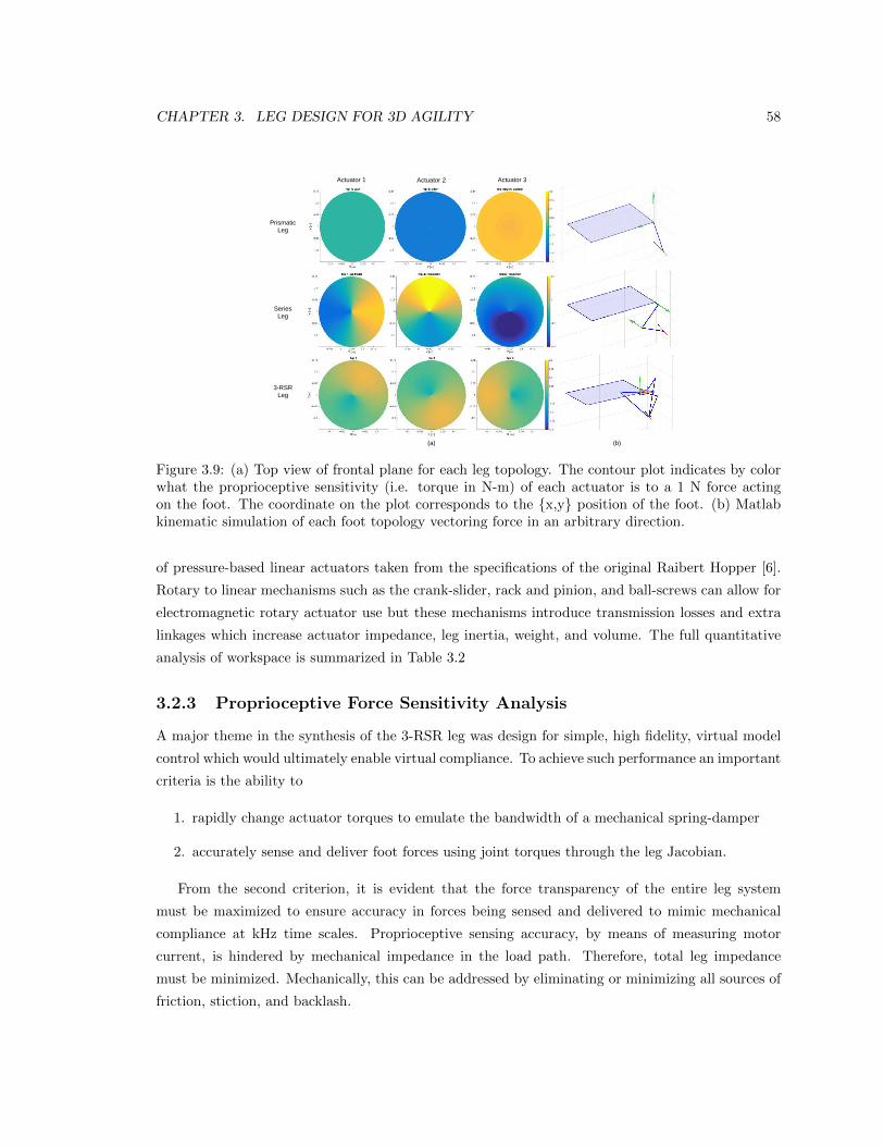
CHAPTER 3. LEG DESIGN FOR 3D AGILITY 58
Actuator 1 Actuator 2 Actuator 3
Series Leg
Prismatic Leg
3-RSR Leg
(a) (b)
Figure 3.9: (a) Top view of frontal plane for each leg topology. The contour plot indicates by colorwhat the proprioceptive sensitivity (i.e. torque in N-m) of each actuator is to a 1 N force actingon the foot. The coordinate on the plot corresponds to the x,y position of the foot. (b) Matlabkinematic simulation of each foot topology vectoring force in an arbitrary direction.
of pressure-based linear actuators taken from the specifications of the original Raibert Hopper [6].
Rotary to linear mechanisms such as the crank-slider, rack and pinion, and ball-screws can allow for
electromagnetic rotary actuator use but these mechanisms introduce transmission losses and extra
linkages which increase actuator impedance, leg inertia, weight, and volume. The full quantitative
analysis of workspace is summarized in Table 3.2
3.2.3 Proprioceptive Force Sensitivity Analysis
A major theme in the synthesis of the 3-RSR leg was design for simple, high fidelity, virtual model
control which would ultimately enable virtual compliance. To achieve such performance an important
criteria is the ability to
1. rapidly change actuator torques to emulate the bandwidth of a mechanical spring-damper
2. accurately sense and deliver foot forces using joint torques through the leg Jacobian.
From the second criterion, it is evident that the force transparency of the entire leg system
must be maximized to ensure accuracy in forces being sensed and delivered to mimic mechanical
compliance at kHz time scales. Proprioceptive sensing accuracy, by means of measuring motor
current, is hindered by mechanical impedance in the load path. Therefore, total leg impedance
must be minimized. Mechanically, this can be addressed by eliminating or minimizing all sources of
friction, stiction, and backlash.

CHAPTER 3. LEG DESIGN FOR 3D AGILITY 59
Actuator 1 Actuator 2 Actuator 3
Series Leg
Prismatic Leg
3-RSR Leg
Figure 3.10: Side view of the sagittal plane for each leg topology. The contour plot indicates by colorwhat the proprioceptive sensitivity (i.e. torque in N-m) of each actuator is to a 1 N force acting onthe foot. The coordinate on the plot corresponds to the y,z position of the foot.
Proprioceptive sensing is also also dependent strongly on leg topology which determines the
Jacobian. Because the transpose of the leg Jacobian relates foot forces and joint torques, an ideal
leg topology for accurate proprioceptive sensing will have a leg Jacobian with a high sensitivity
in joint torques to changes in foot force. This design insight, in combination with minimizing
mechanical impedance is needed to design limbs with adequate proprioceptive force sensitivity for
virtual compliance.
Figs. 3.9 and 3.10 show — for every foot position in the each limb’s workspace (prismatic, series-
articulated, 3-RSR) — the proprioceptive force sensitivity Π. The contour plot’s color represents
the value of Π, the minimum torque resolution needed to sense a 1N force change at the foot in the
position designated by the (x,y) or (y,z) coordinate of plots 3.9 and 3.10, respectively.
3.2.4 Energy Transfer
Energy delivery is an important metric for legged robots planning to jump explosively or run at
high speeds. During running in humans and animals leg swing speed can reach greater than 1080
degrees per second and leg forces can reach 3 times the weight of the body. Therefore, maximizing
energy delivery and power, defined by leg velocity times leg force is an important metric to consider

CHAPTER 3. LEG DESIGN FOR 3D AGILITY 60
Figure 3.11: Renderings of CAD models for the 3-RSR leg design and actuator modules.
when design for high jumping and running. Table 3.2 summarizes the comparison in performance
and required actuation torque for each of the discussed leg topologies.
3.2.5 Summary
The design of the 3-RSR attempted to balance and optimize many metrics associated with legged
agility and proprioceptive force control. Table 3.2 provides a summary and comparison of the 3-
RSR’s performance metrics as compared to the series-articulated and prismatic leg topologies.
TopologyMax Actuator
Torque [N-m]
Work
Space
Leg
Volume
Foot
Force
Foot
Speed
Limb
Inertia
E Ψ Λ Π
1 2 3 [m3] [m3] [N] [m/s] [kg-m2] [J] [N-m3] [m/s2] [N-m]
Prismatic 0.6 9.1 15.0 .0283 .0006 33.3 2.82 0.111 6.7 .94 37 0.0226
Series 11.2 6.7 22.5 .0395 .0030 36.4 9.65 0.058 7.3 1.44 79 0.0667
3-RSR 9.5 9.5 9.5 .0285 .0171 131.5 2.65 0.015 27.0 3.75 209 0.0506
Note: Max Actuator Torque refers to the maximum torque required to produce the wrench in eq. 3.12 atevery point in a vertical foot trajectory. Leg Volume is the max (worst-case) volume the mechanism can
consume. Foot Forces and Velocities are the average over a vertical leg trajectory. The prismatic leg uses arotary to linear mechanism with a reduction of 1:6.7. Ψ is the value of the workspace volume multiplied by
the average foot force in that workspace.
Table 3.2: Comparison of performance measures for 3-DoF leg topologies.
3.3 Mechanical Design of the 3-RSR
The 3-RSR is mechanically constructed of a hip plate, foot plate and 3 identical legs consisting of
two links that connect the hip to the foot. The kinematic configuration of the leg is shown in Fig.
3.2 where the physical realization of the mechanism is a 3-R-RRR-R or 3-5R, where each R-joint

CHAPTER 3. LEG DESIGN FOR 3D AGILITY 61
R2
R3
R4
Figure 3.12: Knee joint design showing the 3 revolute joints with intersecting axes. Solidworks FEAresults indicate that stresses as high as 123 ksi are present at the bearing support shaft of the distalknee segment with a conservative applied force of 300 N and safety factor of 4. Therefore, thiscomponent is machined from medium carbon steel with 125 ksi yield strength in contrast to mostof the other components which are machined from 7075 Aluminum with 73 ksi yield strength.
denotes a 1-DoF revolute joint. The three motors are coupled directly to their corresponding first
link or through a single stage planetary transmission in the case of QDD actuation. The motor stator
is bolted to the hip structure which is adjustable to accommodate different actuator configurations
(DD or QDD). Link 1 (l1) is double supported by bearings on each side to increase moment loading
capacity. l1 has one rotational degree of freedom about revolute joint axis 1 (R1) in Fig. 3.2 where
the axes of the three hip joints are parallel to the hip plane but phased 120o apart to evenly space
the 3 legs of the 3-RSR.

CHAPTER 3. LEG DESIGN FOR 3D AGILITY 62
(a) (b)
Figure 3.13: FEA was conducted on each component and the two other critical components weredetermined to be (a) the other extended shaft in the knee (R2) and (b) the ankle link which connectsthe foot to the carbon fiber l2 rod. A static analysis was used to determine the maximum expectedforce each part could see and those forces ranging from 75N to 200N were applied in the FEA.
3.3.1 Spherical Knee Joint Design
The knee joint consists of three, 1-DOF revolute joints whose rotation axis intersect at one point as
shown in Fig 3.12. This configuration achieves the mobility of a spherical joint however the range
of rotation about each of the three axis is much larger than that found in typical COTS ball-in-
socket spherical joints. The range of motion for joints R2 and R4 is 360o while the range for R3
is ±90o. A typical COTS ball joint will have one axis with full 360o range of rotation while the
other two axis will have ±35o of rotation [66]. Therefore the use of this RRR knee joint enables a
significantly larger limb workspace that would not have been possible with a commercially available
ball joint. The extended range of motion of the RRR joint allows for the leg to pass through its two
configurations: knee-above-hip and knee-below-hip as shown in Fig. 3.30.
To avoid interference between l1 and l2, and l2 and the motor, an offset was integrated into
the distal knee segment with a fixed angle. Although this fixed-angle offset addresses interference
issues, the trade-off is an increase in bending moment loads, higher stresses, and re-locating the
leg’s point of singularity to occur when the foot is in the middle of it’s workspace as opposed to
having the singularity sit at the distal edge of the workspace (as is the case when the fixed angle
is 0o). The singularity occurs when the foot is in a position that causes the axes of R2 and R4
to align and become coincident — essentially removing a degree of freedom in the knee. When
the leg passes through this singularity at high speeds, vibrations propagate through the mechanism
and peak stresses are generated. This singularity can however be re-positioned to different, less
utilized, regions of the workspace by modifying the fixed angle in the knee offset. Fig. 3.14 shows
the relationship between the fixed knee angle and total angular joint range of the driven link, l1
which is directly correlated to the volume of the workspace. The optimization plot indicated that to
maximize the range of motion for the hip (driven) joint which would allow for a greater workspace
and more energy delivered, the knee joint should have a fixed angle of 130o.
FEA analysis showed that the knee joint as the most stress critical element of the design and

CHAPTER 3. LEG DESIGN FOR 3D AGILITY 63
Figure 3.14: Optimization plot showing the relationship between the fixed knee angle and total hipjoint range.
thus most prone to failure modes. The FEA on the most distal knee segment (with the fixed angle
offset) showed that peak Von-Mises stresses exceeded the yield strength of aluminum during the
most critical loading period which occurs during jumping and landing. Therefore, a medium carbon
steel (McMaster C300 or 1144 steel) with yield strength of 110-125 ksi and high impact resistance
is used to increase resiliency to impact loads reaching 300 N.
To minimize the mechanical impedance of the leg mechanism with force transparency in mind, a
large effort was made to reduce and eliminate all sources of friction in the 15 joints on each 3-RSR
leg. Therefore, rather than the more cost effective use of bushings, each of the 15 joints utilize one
or more bearings to reduce friction while being rated to handle large radial and moment loads seen
at the respective joints. For the knee joint two ball-bearings are housed within the hollow carbon
fiber l1 tube 20mm apart and constrain the shaft of R2 as shown in Fig. 3.12. The middle R-joint
R3, is a clevis joint constructed from a needle roller bearing used to support large radial loads. R3
is always orthogonal to both R2 and R4. The bearing has minimal to no thrust loading so the
shaft is press fit into one side of the clevis and 0.005” delrin (also known as polyoxymethylene or
acetal) shims are used to reduce friction between the inner surfaces of the clevis and pin’s housing.
The large moment loads created by the knee offset also must be reacted by the bearings and the
clevis housing. Therefore, the distal knee R-joint, R4 is designed using two angular contact bearings
arranged back-to-back in an O-configuration to increase the effective fulcrum, and thus moment load
rating, of the bearings. Links l1 and l2 are made from 0.76” diameter (.068” wall thickness) high
modulus carbon fiber tubes (45558-HM Rockwest Composites) to maximize the strength-to-weight

CHAPTER 3. LEG DESIGN FOR 3D AGILITY 64
Figure 3.15: Various mechanical components of the 3-RSR leg including foot, knee, and driven linkl1.
ratio of the links while ensuring leg inertia and mass is kept low.
3.3.2 Hip Design and Actuator Placement
The hip is constructed from two parts that are bolted together during assembly. The two parts have
aligned bolt slots to allow actuators and motors of various width and size to fit within the structure
and drive the leg. The hip was made adjustable so that the leg could be tested using direct-drive,
quasi-direct drive, and series elastic actuators actuators without having to fabricate three separate
hip mounting brackets for each different actuator configuration which would account for 9 relatively
costly components. Instead the two parts can be slid to the desired dimensions and bolted together
to maintain that dimension when assembled on the leg. Several slots are made so that many bolts
can be used to hold the two brackets together under large loads.
3.3.3 Foot Design
The sole of the foot is made of molded urethane rubber from SmoothOn. The rubber acts as a
mechanical damper and shock absorber to filter out very high frequency (> 500 Hz ≈ ωn the natural
frequency of the rubber foot) impulse forces during landing from reaching the planetary-gears.

CHAPTER 3. LEG DESIGN FOR 3D AGILITY 65
3.3.4 Mass Budgeting
The 3-RSR was mechanically designed to maximize strength-to-weight ratio of the unsprung mass
and to minimize leg inertia. The 3-RSR has a total leg mass (hip and actuators included) of 2.5
kg (DD) or 3.1 kg (QDD) not including battery and electronics. The leg has an unsprung leg mass
(ml) of 0.63 kg, and a leg inertia of 0.015 kg-m2. Each of the three actuators is composed of a
0.4 kg T-Motor U10 with a 0.2 kg Matex 1:7 single-stage planetary gear reduction in the QDD
configuration (DD does not have the Matex gear). The QDD actuator mass budget (i.e. the ratio
of actuator mass to total mass) is 48% (DD) and 58%(QDD), compared to Penn Minitaur’s 40%,
MIT Cheetah’s 24%, where higher ratios are ideal for inducing dynamic behaviors [12].
Rather than using fasteners to join all 15 joints to their corresponding links, adhesive bonding
was used to reduce component count and minimize inertia of the unsprung-mass. Joining between
the aluminum and steel joints at the hip, knee, and foot is accomplished via adhesive bonding using
Loctite Hysol E-120HP.
For proper carbon-fiber to aluminum adhesion, surface treatment on the metal is required and
the finish of the carbon fiber must be cleaned and sanded to a fit with tolerance of 0.005” to 0.01”.
Surface treatment by means of abrading and applying an Alodine conversion coating is necessary to
increase the surface energy of aluminum which is hindered by the oxide layer. Bond line thickness
control is also critical as variations in thickness through the bond generates varying strain with
higher peak stresses and thus premature failure. Once the aluminum surfaces are abraded the
adhesive must be applied within minutes before an outer oxidation layer forms and reduces surface
energy again. The Loctite Hysol E-120HP cures within 24 hours but can be heated to accelerate
the curing.
3.3.5 Finite Element Analysis (FEA)
A finite element analysis (FEA) is conducted to determine the appropriate materials for each com-
ponent in the leg. The carbon fiber tubes were chosen to maximize the strength to weight ratio.
Carbon fiber is extremely resilient to bending moments and compression which are the primary
loads acting on the leg segments. Due to the complexity and high cost of fabricating custom carbon
fiber parts the legs joints were chosen to be metal and fabricated using CNC machining. The FEA
results in Fig. 3.12 show that with applied normal force of 300 N in the direction indicated by the
purple arrows, stresses as high as 123 ksi are present at the bearing support shaft. This indicates
a safety factor of 4 in the case of a monopod hopper or of 1.2 in the case of a quadruped landing
from a fall of 3 feet on a single leg. Similarly the most proximal segment of the knee joint also sees
large stresses as a result of a straight offset also added for clearance purposes. The FEA for this
component is shown in Fig. 3.13(a). This part is also chosen to be made from medium-carbon steel.
The last component that was calculated to see high loads was the ankle link, in Fig. 3.13(b). To
decrease stress the cross section of the beam extending from the carbon fiber tube of link 2 l2 was

CHAPTER 3. LEG DESIGN FOR 3D AGILITY 66
made larger. This allowed the material component to be made of aluminum which has a density of
2712 kg/m3 which is roughly a third of the density and therefore mass of steel (7850 kg/m3) [67].
3.4 Actuator Requirements for Omni-Directional Jumping
To select the appropriate combination of motor and single stage reduction, the required torque
for desired static and dynamic motions must be determined. The required foot force for statically
supporting the weight of the body indefinitely in stance is first calculated by
Fstance =mg
nlegs(3.13)
where nlegs is the number of legs in stance.
The foot forces required to produce a vertical jump with desired peak height hpeak can be
determined by first calculating the take-off velocity and then determining the leg and body CoM
acceleration required to achieve the necessary take-off velocity.
Ek =1
2mv2to = mghpeak = Ep (3.14)
where m is the robot’s mass, g is acceleration due to gravity, and hpeak is the apex height reached
during a jump. Solving for the initial take-off velocity vto to achieve a desired jump height hpeak,
vto =√
2ghpeak (3.15)
Given a take-off velocity vto to achieve a peak vertical height of hpeak the leg and COM acceler-
ation afoot can now be solved.
afoot =v2to − v2i
2δz(3.16)
where vi = 0 is the starting velocity of the foot which is assumed to be at rest, and δz is the leg
extension range which is dependent on the vertical workspace of the leg topology. To calculate
δz = δlext I start at the fully contracted leg joint angle limits and end the jumping trajectory 50o
before reaching the joint limits on the fully extended side. This provides a range of motion in the
actuators of 130o and a vertical leg extension of δlext = 0.3 meters.
Finally, given a leg Jacobian JT , calculate the required foot force and individual joint torques
for jumping
Ffoot =m(afoot + g)
nlegs(3.17)
τ = JTFfoot (3.18)
where the Jacobian can be taken at the leg topology’s position of weakest foot-force production.
With the calculated joint torques required for jumping to a max height of hpeak, the appropriate

CHAPTER 3. LEG DESIGN FOR 3D AGILITY 67
actuator design can ensue.
3.5 Quasi-Direct-Drive Actuator
An ideal actuator for dynamic legged locomotion that balances force transparency, torque density,
high speed, energy efficiency, and mechanical robustness was determined by analysis in this thesis
to be the quasi-direct-drive (QDD) actuator. This section describes the mechanical and electrical
design in addition to the low and high level motor controllers developed for GOAT’s custom DD and
QDD actuator. Although DD is employed for GOAT, I argue that QDD is more optimal for purposes
of energy efficiency and real world feasibility of legged robots at the marginal cost of slightly lower
force control bandwidth and proprioceptive sensing accuracy.
3.5.1 Mechanical Design
The custom QDD used on GOAT consists of 4 major components: a Tiger U10 brushless DC motor,
a variable motor bracket/housing which allows different Tiger motors and gearboxes to be used,
a single-stage planetary gear box, and ball-bearings on the motor’s output for double support to
handle large radial and moment loads acting on the rotor.
Although QDD offers advantages in energy efficiency by conserving a factor of n2 power for
a given torque production, the GOAT actuator was designed to be configured as QDD or DD in
which no gearbox is used. Performance tests on the T-motor U10 indicated that these motors in
direct-drive mode are capable of producing sufficient torque at speed (i.e. power) to induce explosive
jumping given the minimized weight and inertia of the leg design. Therefore, both DD and QDD
actuation schemes will be experimentally tested on the GOAT leg.
Motor
Motor selection to drive the QDD or DD actuator was based on maximizing thermal specific torque.
It was determined in [12] that the T-motor U8, and more generally the U-Power Series, had superior
torque density as compared to other commercial off-the-shelf (COTS) motors. The Maxon EC-90
Flat was considered because of the convenience in using a Maxon based motor driver but the torque
density of this motor, due mostly to added mass from a fully enclosed stator housing/frame, was
not sufficient. Therefore, a Tiger motor U10 was chosen.
Transmission
To increase the torque density of the GOAT leg’s actuators, a single stage gear stage can be placed
between the motor and the drive hip link. In previous sections it was shown that adding a single
stage gear transmission, specifically a single-stage planetary, would decrease energy requirements for

CHAPTER 3. LEG DESIGN FOR 3D AGILITY 68
Figure 3.16: The Tiger Motor U10 shown here has a large 40 mm gap radius and a lightweight frame.The T-motor U8, U10, and U12 were determined to have one of the highest thermal specific torquesof any COTS motor (0.42 Nm
kgCo at rgap = 40 mm) [43]. For reference the custom MIT cheetah motors
have a thermal specific torque of 0.71 NmkgCo at rgap = 49 mm [9].
generating a desired torque by allowing the motor to operate in a more efficient regime with lower
current and thus lower Joule heating losses and less saturation from thermal management or RMS
limiting. A single stage planetary transmission was shown to mitigate many of the common negative
effects of geared transmissions as it is able to maintain a bandwidth of 40 Hz and proprioceptive
torque sensing within 6% error.
Housing
The adjustable housing of the actuator also serves as part of the hip structure in the 3-RSR leg
design. The 2-piece actuator mounting brackets can be seen in Fig. 3.17. The housing consists of
two components which allow the motor to be bolted on to one end while the link 1 bearings are
press fit into the other end. This design allows the motor rotor and link 1 to be double support (o.e.
support from both sides) for higher radial load rating.
3.5.2 Electrical Design
Three printed circuit boards are used for the total actuator module. The module includes a motor
driver board based off a TI Piccolo TMS320F28069M MCU and a DRV8301 Bridge Driver which
drives 6 N-channel Vishay SUM110N06-05L 60 V MOSFETs with 175oC temperature limit. This
board is responsible for running the low level motor commutation and PID controllers for separate
position, velocity, and torque control at 10 kHz. The board has a built in AMS AS5048A magnetic
encoder which senses the change in magnetic field from a diametrically polarized magnet connected

CHAPTER 3. LEG DESIGN FOR 3D AGILITY 69
Figure 3.17: The quasi-direct-drive actuator module driven by a T-motor U10 with a single stageMatex 1:7 planetary gear stage.
to the axle of the rotor. The second custom board is currently a modified Hebi prototyping I/O
board with various input/output channels including SPI, I2C, Serial, and Ethernet. This board is
designated for communications and data transfer/exchange between the motor controller board and
a main computer sending high-level commands. The third board is a small encoder board placed
on the output side of the actuator to measure absolute output angle using the same AMS AS5048A
magnetic encoder and sensing the magnetic field of a permanent magnet in the shaft of the driven
output link 1. This is needed when the actuator is configured in QDD mode to have knowledge of
absolute output position after the gear stage.
The power electronics are capable of energy regeneration to convert work done on the leg back
into battery potential for added efficiency. The exact mechanical to electrical energy conversion was
not measured but for reference the MIT Cheetah’s custom electronics achieve 63% energy efficiency
during this conversion [9].
3.5.3 Actuator Control
Optimal Motor Commutation: Field Oriented Control
A custom motor controller was required for the desired control of the brushless DC Tiger U10
motor. COTS electronic speed controllers used to power similar motors for quadrotors use back-
EMF or hall effect sensors to electronically commutate the motor and cyclically energize the motor
windings. These off-the-shelf ESC’s are designed for velocity control and driving brushless motors at
high speeds in a single direction. They are inadequate for direct-drive application requiring precise
position and torque control over the entire spectrum of rotor velocities.

CHAPTER 3. LEG DESIGN FOR 3D AGILITY 70
Figure 3.18: Custom GOAT motor driver configured with a Piccolo TMS320F28069M MCU and aDRV8301 Bridge Driver which drives 6 N-channel Vishay SUM110N06-05L 60 V MOSFETs with175oC temperature limit.
Figure 3.19: The custom Hebi Robotics communications board outfitted with a 32-bit ARM Cortexprocessor, Ethernet switch, and SPI port among other I/O ports for prototyping.
The main methods of brushless motor commutation are 6-step square wave, sinusoidal, and field-
oriented control. Of these three, 6-step square wave is the simplest – using only a look-up table
based on feedback from 3 hall effect sensors placed on the stator used to determine the rotor position
sextant. Based on the electrical angle of the rotor six hall effect states can exist, in which one phase
winding sources current, one sinks current, and one is neutral. Each hall-effect state corresponds to
CHAPTER 3. LEG DESIGN FOR 3D AGILITY 71
Electrical Angle [o] Hall Effect State Phase A Phase B Phase C0-60 0,0,1 + - neutral
60-120 0,1,1 + neutral -120-180 0,1,0 neutral + -240-300 1,1,0 - + neutral180-240 1,0,0 - neutral +300-360 1,0,1 neutral - +
Table 3.3: Lookup table for six-step square commutation [47].
a specific energizing state for the three phase windings according to Table 3.5.3 [47].
Alternatively, sinusoidal commutation energizes the 3 windings with 3 identical sinusoidal waves
phase shifted apart from one another by 120o electrical. Each sinusoidal phase current is generated
by pulse width modulation (PWM) from the motor controller. This creates a N/S electromagnetic
field that rotates within the motor core. Sinusoidal commutation reduces torque ripple and cogging
as compared to 6-step square wave but it requires finer angular position feedback of the rotor for
direct-drive position controlled applications. Therefore, an encoder is needed to get precise rotor
angle feedback. Sinusoidal commutation would theoretically produce maximum torque at every rotor
angle without ripple or cogging if current was in phase with voltage.
Field-oriented control (FOC) or vector control is the most complex commutation method and it
closes the feedback loop on motor current rather than voltage to address the issue of current lagging
being the commanded phase voltages which is an inherent effect of the motor’s inductance. This
is explained by a simple motor model which is composed of a speed dependent voltage source (i.e.
back-emf) in series with a resistor and inductor. For a 3-phase motor the resistance is the resistance
of each phase winding and the inductor is the inductance caused by the winding coils which naturally
opposes change in current and thus causes a phase-shift between commanded voltage sinusoid and
the current response.
Because a magnetic field is generated by current flowing through a coil (not voltage), and current
is out-of-phase with voltage in AC circuits, the torque (via current) if out-of-phase from the voltage
will be less than optimal at any given rotor angle.
Fig. 3.20 from [56] shows the magnetic force and torque production for three different phase
alignments of the rotor’s permanent magnet and the stator’s electromagnetic fields. In the non-
optimal case the magnetic force is made up of two components of which only one is acting to produce
torque. The larger the phase shift between the voltage and current, the larger the component of the
magnetic force that pulls outward ( direct current) in comparison to the component which produces
torque (quadrature or Torque current). This phase-shift not only decreases torque but wastes power
and increases torque ripple.
Therefore, FOC measures the two components of current, direct Id and quadrature Iq, and

CHAPTER 3. LEG DESIGN FOR 3D AGILITY 72
(a) (b)
(c) (d)
Figure 3.20: (a) is a simple motor model showing torque production for three different phase align-ments of the rotor’s permanent magnet and stator’s electromagnetic fields. (b) shows a decompo-sition of magnetic force or pull direction into two components: one that produces torque and onethat pulls outward and wastes energy. The purpose of FOC is to continuously apply a magneticfield in the stator windings which converts all the magnetic force into the component that producestorque. (c) shows the phase-shift that exists between phase winding voltage and phase current,which is around 20o here. (d) shows the commanded voltage sinusoids vs. electrical angle and thecorresponding magnetic field produced by the energized windings. Figure source: [56].
adjusts the voltage phase to minimize Id and maximize Iq for maximum torque production. This
control is achieved by closing the loop on current via sensing of the AC current on two of the
three phase windings5. The three AC phase currents are then transformed using the Clarke and
Park transformations with encoder feedback to measure the direct and quadrature current, Id and
Iq, in the rotors rotating frame. Transforming AC phase currents ia, ib, and ic into DC Id and
Iq simplifies the PI control around current because the DC currents have significantly less time-
variation and aren’t cyclic and sinusoidal [56]. Two PI controllers then modulate the phase and
voltage applied to each phase winding so the commanded Id and Iq current are achieved. For the
GOAT actuator Iq is set to zero to maximize the torque production of the motor at low speeds. Iq
is sometimes increased from zero in order to reach very high operating speeds. Fig. 3.21 from [56]
is a simplified schematic of how the PI controller modulates the PWM voltage signal so that direct
current is eliminated and quadrature current is maximized to reach the desired torque. In addition
to maximizing torque output, FOC minimizes torque ripple, cogging, energy loss, and Joule heating
due to flux current used to pull the rotor outward rather than produce torque.
A step by step algorithm on how to implement the well known FOC method is now briefly
described according to [68]. The algorithm references variables found in Fig. 3.22.
5the third phase current is calculated from Kirchoff’s current law (KCL) for wye-configured windings

CHAPTER 3. LEG DESIGN FOR 3D AGILITY 73
(b) (a)
Figure 3.21: (a) is a flow chart showing the FOC commutation. (b) is the control strategy whichminimizes Id and maximizes Iq. Figure source: [56].
Figure 3.22: Representation the input (a, b, c) winding reference frame and the rotating d− q framefor a 4-pole brushless motor.

CHAPTER 3. LEG DESIGN FOR 3D AGILITY 74
Algorithm 1: Field Oriented Control [68]
1: procedure FOC(Iq,cmd, Id,cmd)2: Measure the 3 stator phase currents convert them to complex state space vector (a,b,c)
coordinate system3: Current vector is converted to (α, β) 2-axis stationary coordinate frame using Clarke
Transform where ia, ib, ic are the time varying AC currents of each stator winding.
Iα,β,γ(t) = Tia,b,c(t) =2
3
1 − 12 − 1
2
0
√32 −
√32
12
12
12
iaibic
(3.19)
and if ia is superimposed and aligned with Iα and a wye winding configuration is used such thatia + ib + ic = 0 then the transform is simplified to
Iα = ia (3.20)
Iβ =1√3
(ia + 2ib) (3.21)
4: Use the Park Transform to transform the (α, β) stationary reference frame to (d, q), therotating reference frame. The coordinate frame is aligned such that the d-axis passes througha north rotor PM pole and the q-axis is 90o electrical (defined by PM poles) in the direction ofrotation or applied torque. For example a 2 pole motor the q-axis is displaced 90o mechanicalfrom the d-axis of the rotor; for a 4 pole motor it is displaced 45o mechanical from the d-axis.
Id = Iα cos θ + Iβ sin θ (3.22)
Iq = Iβ cos θ − Iα sin θ (3.23)
where Id is the flux/outward pull component of current and Iq is the torque producing componentof current.
5: Run a PI controller on the commanded currents Iq,cmd, Id,cmd in this d-q rotating frame.6: The PI controller modulates the voltage components in the d-q rotating reference frame,
therefore it must be converted back to reference voltage wave forms in the stationary (a, b, c)frame. First use the Inverse Park Transform to transform d-q currents to the stationaryα− β reference frame by
Vα = Vd cos θ − Vq sin θ (3.24)
Vβ = Vq cos θ + Vd sin θ (3.25)
7: Penultimately use the Inverse Clarke Transform to convert back from orthogonal 2-axisframe (α, β) to 3-phase stator frame (a, b, c).
Va = Vα (3.26)
Vb =1
2(−Vα +
√3Vβ (3.27)
Vc =1
2(−Vα −
√3Vβ (3.28)
8: Finally, using PWM apply the 3-phase voltages (Va, Vb, Vc) to generate the commanded cur-rents and thus torque while accounting for the voltage-current phase-lag due to motor inductance.

CHAPTER 3. LEG DESIGN FOR 3D AGILITY 75
Figure 3.23: Output of the RMS current limiter which monitors the RMS current and saturates thecommanded output torque when necessary to remain within the motor winding’s thermal limits.
Thermal Management and Control
The current system was experimentally determined to be thermally limited by the thermally limiting
hardware on the bridge driver board which saturates the FETs at 150oC. Once the FETs reach their
thermal limits the bridge driver saturates current to the phase windings. With the current hardware
the bridge driver reaches higher temperatures than the motor windings. The future, custom designed,
motor driver board will integrate a finned heat sink on each FET to increase surface area for unforced
convection which will dissipate heat faster. Additionally an aluminum plate can be added to the
underside of the board to sink heat from both sides.
To maximize performance yield from the T-motor the motors are not limited by voltage but
rather by an RMS current monitor which tracks the RMS value of the current history and saturates
the current output commanded to the motor if the RMS value exceed the continuous rated current.
The RMS current limiter ensures in a round about way that thermal limits of the windings are
not exceeded. While thermal modeling and feedback using a thermocouple on the stator winding

CHAPTER 3. LEG DESIGN FOR 3D AGILITY 76
Figure 3.24: Thermal analysis showing the time response in winding temperature to 4 commandedtorques ranging from 1.19 N-m to 2.85 N-m with associated thermal time constants. Thermal timeconstant was calculated by 63% of the time taken to reach steady-state. If steady state was notreached the maximum temperature was used. A FLIR E40 Infrared Thermal Imaging Camera wasused to collect real-time temperature data on the windings.
Figure 3.25: A FLIR E40 Infrared Thermal Imaging Camera was used to observe the temperaturegradient over the motor windings and the PCB containing the motor driver FET bridges. (a) is atop-view IR image of the torque test rig with the motor driver PCB (cursor 1) and the T-motor(cursor 2). (b) shows a closer view of the T-motor U10. The thermal image depicts which statorwinding poles are being energized and the temperature at those windings.
would be more accurate, it is also more complex and requires outfitting the motor with additional

CHAPTER 3. LEG DESIGN FOR 3D AGILITY 77
sensors and ensuring those sensors remain operational. RMS current limiting requires not additional
sensors beyond current sensing which is already needed for motor commutation. Additionally, for
thermal modeling multiple temperature sensors placed around the stator windings must be used
to accurately measure max winding temperature as some windings may be highly energized while
other are not (as seen in Fig. 3.25) which may lead cause the thermal management system to fail
in saturating current when necessary.
A thermal analysis was conducted to measure the time response in winding temperature to 4
commanded torques ranging from 1.19 N-m to 2.85 N-m from which the associated thermal time
constants were determined. Thermal time constant was calculated by 63% of the time taken to reach
steady-state. If steady state was not reached the maximum temperature was used. A FLIR E40
Infrared Thermal Imaging Camera was used to collect real-time temperature data on the windings.
The thermal time constant for 1.3 times and 2 times the continuous rated current was determined
to be 28.1 and 6.2 seconds respectively. Therefore, to match the thermal profile of the T-motor the
RMS current limiter was set to have a history window or period of 60 seconds and a continuous
rated current of 1.45 N-m. The time window over which RMS is calculated (60 s) was chosen based
on thermal tests using thermal camera, Fig. 3.25, and watching how long it took the windings to
reach their thermal limits at different constant torque values. The RMS period was calculated so
that it matched the thermal time constant and would saturate the signal right before the windings
reached their thermal limits. If the RMS period is set to be too long there is a risk of burning out
the motor due to excessive Joule heating which melts the winding insulation. The T-motor uses
class F insulation which is rated at 100oC rise from ambient or an absolute operating temperature
of 155oC.
Communications
The T-motor DD and QDD actuator module run custom low level firmware for FOC commutation
at 25 kHz and the PID loops for separate position, velocity, and torque control at 10 kHz all on
board a TI Piccolo TMS320F28069M micro-controller unit (MCU).
The schematic in Fig. 3.26 shows the communications layout of the hardware. High level
commands and the motion planner are computed in real-time on a lap-top computer using MATLAB.
Position, velocity, and torque commands and associated gains are sent at 1 kHz over 100 Mbps
Ethernet using TCP/IP to a communications board. The communications board manages data
transfer between the lap-top and the Motor Driver board. The comm board uses a 32-bit ARM
Cortex processor to handle Ethernet communications and SPI transfer. The SPI protocol is used
to communicate between the Comm board and the TI motor driver. This data transfer line passes
commands and sensor feedback between the TI motor controller and the laptop. The motor driver is
a TI 3-phase brushless DC motor driver running on a Piccolo MCU with a DRV8301 bridge driver.
Custom firmware is uploaded onto this board to drive the T-motor using position, velocity, and

CHAPTER 3. LEG DESIGN FOR 3D AGILITY 78
Figure 3.26: Schematic wiring diagram of the electronics for a single GOAT actuator.
torque commands. The motor driver then inverts the DC power into an AC power which is sent to
the 3-phase motor. A custom PCB with integrated magnetic encoder reads a diametrically polarized
permanent magnet coupled to the rotor and relays this feedback to the TI board over ABI.
Calibration
Calibration of the T-motor was accomplished using the same 1-axis SRI M2210E torque load cell.
From the calibration the motor’s torque constant was determined as well as the control constant
which is an internal value in the custom created Matlab API for commanding the motor.
Figure 3.27 shows a torque vs current plot of the motor the torque constant to be 0.072 N−mA . The
magnetic flux in the motor core begins to saturate at 70 A and the thermal limits of the motor driver
half-bridges reach their thermal limits between 75-80 A. The shaded color zones indicate allowable
duty time and duration of holding torque. The green region indicates infinite holding as this region
is within the continuous current and thermal limits of the motor; green-yellow corresponds to duty
times ranging from 5 minutes to 20 seconds; yellow indicates short duty cycles of up to a few seconds;
orange indicates duty cycles less than 1 second; and red indicates peak instantaneous torques with
a duty cycle of a few milliseconds.
The calibration with the MATLAB API motor controller was found to be 0.103 [N-m/Unit] using
data from the plot in Fig. 3.28. The colored regions in Fig. 3.28 correspond to the same operating
regimes as those described for Fig. 3.27.

CHAPTER 3. LEG DESIGN FOR 3D AGILITY 79
Figure 3.27: A torque vs current plot of the motor shows the torque constant to be 0.072 N−mA . The
magnetic flux in the motor core begins to saturate at 70 A and the thermal limits of the motor driverhalf-bridges reach their thermal limits between 75-80 A. The shaded color zones indicate allowableduty time and duration of holding torque. The green region indicates infinite holding as this regionis within the continuous current and thermal limits of the motor; green-yellow corresponds to dutytimes ranging from 5 minutes to 20 seconds; yellow indicates short duty cycles of up to a few seconds;orange indicates duty cycles less than 1 second; and red indicates peak instantaneous torques witha duty cycle of a few milliseconds.
Figure 3.28: Torque calibration to determine the relationship between the commanded value in thecustom motor-controller Matlab API.

CHAPTER 3. LEG DESIGN FOR 3D AGILITY 80
3.6 Sensing
Beyond motor current sensing there are six 14-bit on axis magnetic rotary position encoders (Austria
Microsystems AS5047P) mounted on a custom PCB of which three are used for motor commutation
and mounted to the back of the T-motor U10 stator frame. The AMS AS5047P magnetic encoder
chip is able to operate within close proximity to the motor (considering the strong time-varying
magnetic field generated by the motor) by canceling out all external magnetic fields (where ’external’
refers to any magnetic field not created by the diametrically polarized magnet fixed to the rotor shaft)
by built-in magnetic immunity. This immunity is achieved by using 4 hall sensors within the encoder
chip with software that uses two pairs of differential measurements to calculate the magnetic field
of the encoder magnet which relates to rotor angular position. Therefore, any external magnetic
fields existing are canceled by the differential measurement using the reasonable assumption that
any external fields will have the same field strength on all 4 hall sensors which are very closely spaced
in comparison to the size of the motor [69].
The other 3 are placed on the actuator housing and measure the angular position of the output
shaft in the case a gearbox is used. The output of the actuators are rigidly coupled to their respective
link 1’s l1. The encoders used for motor commutation are placed 2mm axially from the diametrically
polarized permanent magnet which is mounted to the rotor axle. Similarly, three diametrically
polarized permanent magnets are embedded in link 1 (l1) on the motor output axis at a distance
of 2 mm from the encoder located on the output side of the actuator housing. The encoder has
a resolution of 0.08 degrees ( 360214 ), communicates over SPI to an Arduino which uses an Ethernet
shield to transfer data to Matlab environment with real time feedback at 1 kHz.
3.7 Experiments
3.7.1 Complete System
For preliminary testing the GOAT leg is constrained to a 1-DoF test rig using a 15.5 mm wide linear
bearing and guide rail. This setup only allows the leg to move in the vertical direction. All electronics
and power are mounted off-board currently, although the custom electronics described previously
are currently being developed for on-board mounting. The electronics and battery are expected to
add a mass of 1 kg (0.75 kg for battery and 0.25 kg for electronics). Figs. 3.31 and 3.32 show the the
complete GOAT leg mounted on the 1-DoF test rig. A video of preliminary experiments introducing
the GOAT leg demonstrating virtual compliance, hopping, explosive jumping, and omni-directional
running trajectories can be found here: https://www.youtube.com/watch?v=n319xVomJTQ.
The full leg mechanism was tested to determine the mechanical friction present in the system.
Equal joint torques were commanded at each of the three hip actuators starting at zero and increasing
until motion in the leg was seen. The torque at each actuator was found to be around 0.063 N-m

CHAPTER 3. LEG DESIGN FOR 3D AGILITY 81
when the leg began to to move. This is compared to the static friction in each motor of around
0.048 N-m indicating minimal added friction in the actual mechanism. This can be attributed to the
high quality bearings composing each of the 15 joints and the use of shims between all surfaces with
any sliding contact. This equates to approximately a 1 N force at the foot which means that forces
less than 1 N would be difficult to measure using proprioception through motor current. There is
however some backlash in the mechanism – in the clevis joint and in the ankle joints — which could
not be easily removed even with the use of shims between sliding surfaces. Although this can be
most likely be improved by higher machining tolerances, the sub-1-mm backlash in the system seems
negligible in terms of its effect on the performance of jumping and landing using virtual compliance.
3.7.2 Omni-Directional Force Vectoring with Force Plate
In section 3.2 the 3-RSR topology was shown to be superior in terms of requiring the least amount
of joint torque per actuator to generate omni-directional force-torque wrenches. To experimentally
validate that the 3-RSR could, in fact, deliver force equally well in all vectors in the frontal plane as
it could in the sagittal plane a test which commanded the leg to generate 18 force-torque wrenches
defined by eq. 3.12 where θ ranged from 0 to 360 in increments of 20 degrees while on a 1-DoF
test rig. The resulting data, Fig. 3.29, collected by a 6-axis AMTI OR6-7-2000 force-torque plate
show that the magnitude of force produced in the x direction is equal to the magnitude of foot force
produce in the y direction. This indicates that the 3-RSR is capable of generating foot forces out of
the sagittal plane equally as well as it can generate force in the sagittal plane. This is done using less
torque in the 3-RSR leg than in other topologies while also demonstrating enhanced experimental
mechanical robustness in delivering out-of-sagittal plane forces.
3.7.3 Omni-Directional Running
To test omni-directional running and walking ability, the GOAT leg was fixed on a 1-DoF test rig so
that the foot could not touch the ground. The foot was then commanded through a minimum jerk
spline trajectory for omni-directional running. The leg was able to reach high running speeds with a
stride length of 0.25 m at 2.4 Hz. A video showing seamless changes in running direction as well as
high speed running trajectories can be found here: https://www.youtube.com/watch?v=n319xVomJTQ.
3.8 Summary and Design Insights of the GOAT leg
This section highlights and summarizes the key design insights and advantages that the novel 3-RSR
GOAT leg offers with respect to other, more common, leg topologies. The GOAT leg
1. seems (from preliminary experimentation) to be relatively mechanically robust to
large 3D forces and even large falls. The leg was never broken during any of the
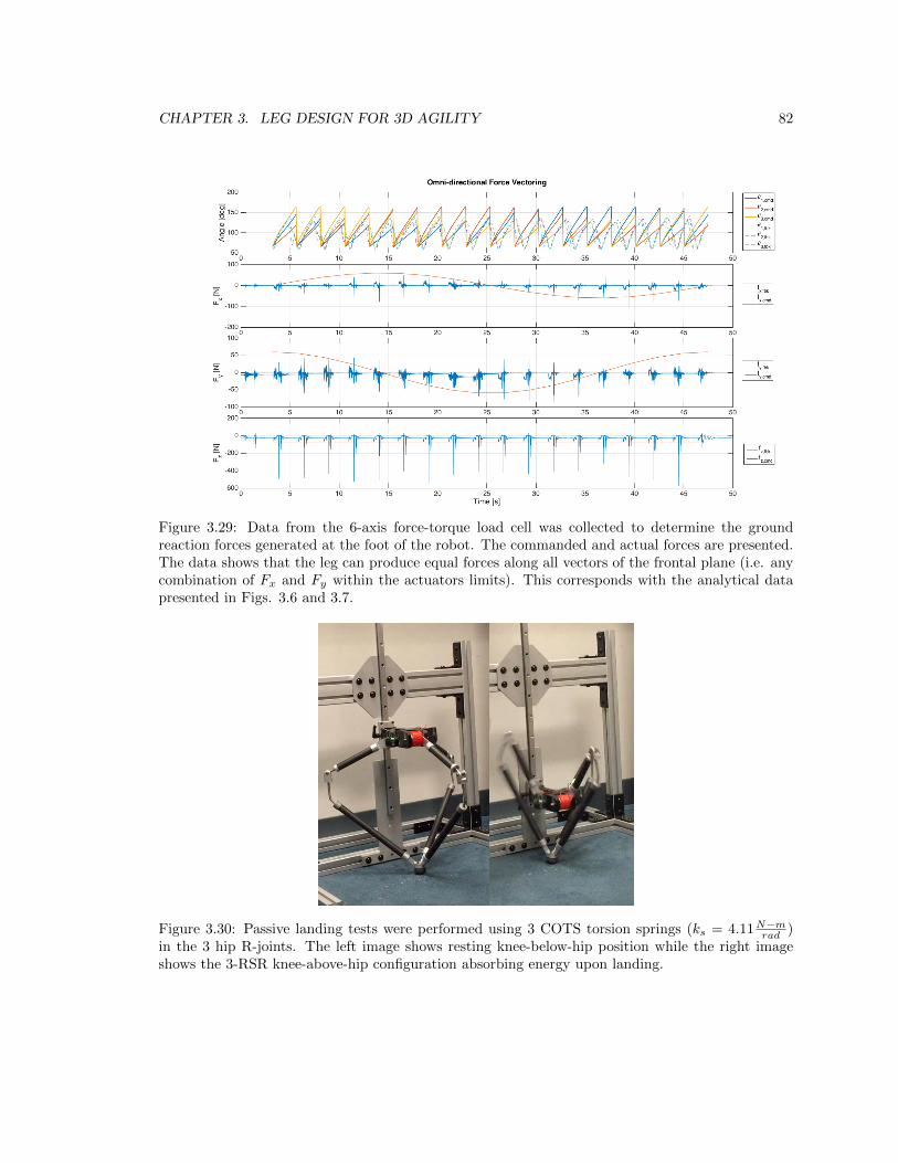
CHAPTER 3. LEG DESIGN FOR 3D AGILITY 82
Figure 3.29: Data from the 6-axis force-torque load cell was collected to determine the groundreaction forces generated at the foot of the robot. The commanded and actual forces are presented.The data shows that the leg can produce equal forces along all vectors of the frontal plane (i.e. anycombination of Fx and Fy within the actuators limits). This corresponds with the analytical datapresented in Figs. 3.6 and 3.7.
Figure 3.30: Passive landing tests were performed using 3 COTS torsion springs (ks = 4.11N−mrad )
in the 3 hip R-joints. The left image shows resting knee-below-hip position while the right imageshows the 3-RSR knee-above-hip configuration absorbing energy upon landing.

CHAPTER 3. LEG DESIGN FOR 3D AGILITY 83
Figure 3.31: GOAT Leg prototype with T-motor U10 actuators mounted in direct-drive configura-tion.
high jumping, landing, and hopping tests.
2. was analytically and experimentally shown to be capable of generating omni-
directional force-torque wrenches at the foot with less required torque per actuator
than the other leg topologies.
3. requires less torque per actuator and distributes foot loads over multiple actua-
tors enabling the use of direct-drive and quasi-direct-drive actuation to achieve
both explosive power and high fidelity proprioceptive force sensing for virtual
compliance.
4. has optimized leg parameters which increase its workspace to encompass most
of the required workspace for legged locomotion including walking, running, and
jumping.
5. has very low limb inertia inertia as compared to all current legs as all the actuators’
stators are static and fixed to the hip frame. This means that the mass of the
actuators does not contribute to the inertia of the leg like in the MIT Cheetah
and other serially configured designs.
The GOAT leg has proven itself to be a mechanically robust 3D parallel mechanism with 3
degrees of freedom which allow it to exert force equally along any vector in the frontal plane with
less required torque than would be required by the prismatic, series articulated, and parallel planar

CHAPTER 3. LEG DESIGN FOR 3D AGILITY 84
Figure 3.32: GOAT Leg prototype and experimental 1-DoF vertical jumping test bed. Electronicsand power (LiPo battery — blue) are both shown in the bottom right image off-board, as tested.The gray ground plate the robot is standing on is a 6-axis force-torque load cell.
topologies6. While series-articulated limbs can use one large actuator at the knee7 for sagittal plane
jumping and tilt the entire leg to produce out-of-plane forces, the leg structure is, similarly, not
designed to bear high lateral forces. Additionally, for the series-articulated and prismatic limbs to
produce forces at vectors which do not pass directly through the hip joint, much larger torques from
the hip abduction/adduction actuator as well as the hip flexion/extension actuators are required.
Therefore, if these actuators are made small — assuming the knee actuator will bear the brunt of
the loads required for jumping — then the prismatic and series articulated leg topologies would
be much weaker in producing omni-directional force vectors at any spot within their workspace as
compared to the 3-RSR GOAT leg.
Also, by relying on a single actuator to carry the load for jumping as done in the prismatic and
6The parallel planar topology in ATRIAS is only extended to the third dimension using an abduction joint andthus the parallel mechanism portion of the leg is planar while the entire leg is made spatial. The fact that the parallelmechanism is planar makes ATRIAS’ legs very susceptible to failure due to lateral (or out of sagittal plane forces).
7the knee joint actuator is responsible for leg extension/thrust while the hip actuator is responsible for leg angleswing. This decoupled actuation is inherent to both series-articulated limbs and prismatic limbs

CHAPTER 3. LEG DESIGN FOR 3D AGILITY 85
series-articulated limbs, that actuator must almost certainly be outfitted with a transmission to pro-
duce required torques/forces. This comes at the sacrifice of an unequally distributed proprioceptive
force sensitivity from each actuator. Therefore, it is important to note that a parallel leg topology
which distributes foot loads over multiple actuators does not need to sacrifice proprioceptive sensing
accuracy (by adding a transmission) for agility.
While the GOAT leg will most likely never be faster than the very impressive speeds achieved by
the MIT Cheetah in running along a straight line, the design of GOAT sacrifices 1D top speed for
the potential to run and jump in all 3 dimensions with more agility than the MIT Cheetah and all
other dynamic legged robots to this date. The design of legged robots at this point is clearly task
optimized and as such it is not entirely fair to compare the GOAT leg to the MIT Cheetah. This
is because the MIT Cheetah was initially designed with biomimetic intentions and attaining high
running speeds rather than focusing on 3D agility via omni-directional running and jumping.

Chapter 4
Proprioceptive Force Control for
Dynamic Virtual Compliance
4.1 Simple Legged Locomotion Controllers
The 3-RSR was designed for high fidelity proprioceptive force control to enable a leg with mechani-
cally variable spring stiffness and dampening to be emulated by virtual compliance from electromag-
netic actuators driving a stiff leg structure. To understand why variable compliance is important
in legged locomotion the SLIP model and Raibert controller are described. Both legged models of
locomotion assume some level of compliance in the hopping leg. Variable stiffness is also important
with regard to energy efficiency at different running/hopping speeds and over terrain of varying
stiffness [64][21].
4.1.1 SLIP Models
From observing cursorial creatures in nature scientists have long known that the muscles and tendons
of running animals acts as springs and dampers to store and deliver energy in each gait cycle. While
many robots use designs integrating passive mechanical elements such as leaf springs into the leg
mechanism few robots have achieved virtual compliance at the kHz time scale required for smooth
spring emulation via electromagnetic actuators [9][12][11].
The purpose of the 3-RSR leg topology and associated quasi-direct-drive scheme aim to enable
high fidelity virtual model control to enable the mechanically stiff leg to act like a spring upon
landing impacts prevalent in hopping. Therefore, for reference, this document includes the well
known derivations of 1-DoF and 2-DoF spring-loaded-inverted pendulum (SLIP) model which is one
of the simplest yet most powerful models of dynamic legged locomotion [61]. Each model has two
distinct dynamics equations of motion for stance phase and flight phase.
86

CHAPTER 4. PROPRIOCEPTIVE FORCE CONTROL FORDYNAMIC VIRTUAL COMPLIANCE87
1-DOF SLIP Model
The one degree of freedom model taken from [61] describes the motion of a monopod hopper with a
mass-less spring leg of stiffness k and an effective body point mass m. The point mass is constrained
to motion only in the y-direction as indicated by Figure 4.1. The model assumes
1. mass-less/inertia-less limb
2. center of mass (CoM) located at the hip
3. ideal linear spring leg with no dampening
The stance phase dynamics are derived using Newton’s 2nd law by summation of force acting
on the point mass while the foot is in contact with the ground as follows [61]
my = k(l0 − y)−mg (4.1)
where l0 is the unstretched spring-leg length. The state space variable x is then defined as
x =
[y
y
](4.2)
x1 = y = 0 (4.3)
x2 = y =k
m(l0 − y)− g (4.4)
The dynamics equations of motion for the stance phase are then written in state-space form as[y
y
]=
[0 0
− km 0
][y
y
]+
[0
km l0 − g
](4.5)
The flight phase dynamics are much simpler as the only force acting on the body mass is gravity.
Therefore, the trajectory of the mass follows ballistic flight described by
my = mg (4.6)
y = g (4.7)
2-DOF SLIP Model
The 2-DoF SLIP model from [61] is an extension of the same model which adds horizontal translation
to the point mass body motion. This enables hopping in a plane as opposed to a vertical line. The
same simplifying assumptions used for the 1-DoF model apply.
Using the Lagrangian formulation the system dynamics for the 2-DoF model stance phase can
be determined. Taking the difference between the systems kinetic T and potential V energy yields
L = T − V (4.8)
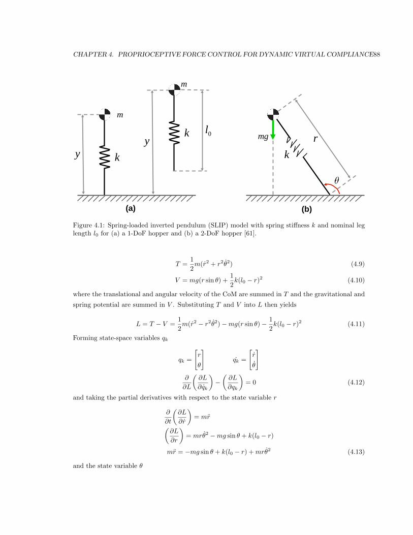
CHAPTER 4. PROPRIOCEPTIVE FORCE CONTROL FORDYNAMIC VIRTUAL COMPLIANCE88
rmg
ky
m
k
ky
m
l0
(a) (b)
Figure 4.1: Spring-loaded inverted pendulum (SLIP) model with spring stiffness k and nominal leglength l0 for (a) a 1-DoF hopper and (b) a 2-DoF hopper [61].
T =1
2m(r2 + r2θ2) (4.9)
V = mg(r sin θ) +1
2k(l0 − r)2 (4.10)
where the translational and angular velocity of the CoM are summed in T and the gravitational and
spring potential are summed in V . Substituting T and V into L then yields
L = T − V =1
2m(r2 − r2θ2)−mg(r sin θ)− 1
2k(l0 − r)2 (4.11)
Forming state-space variables qk
qk =
[r
θ
]qk =
[r
θ
]∂
∂L
(∂L
∂qk
)−(∂L
∂qk
)= 0 (4.12)
and taking the partial derivatives with respect to the state variable r
∂
∂t
(∂L
∂r
)= mr(
∂L
∂r
)= mrθ2 −mg sin θ + k(l0 − r)
mr = −mg sin θ + k(l0 − r) +mrθ2 (4.13)
and the state variable θ

CHAPTER 4. PROPRIOCEPTIVE FORCE CONTROL FORDYNAMIC VIRTUAL COMPLIANCE89
∂
∂t
(∂L
∂θ
)= mr2θ(
∂L
∂θ
)= −mgr cos θ
r2θ = gr cos θ (4.14)
The flight phase dynamics are again described by ballistic flight
y = g (4.15)
x = 0 (4.16)
The following system of equations is nonlinear and thus can be easily solved numerically, how-
ever an additional assumption simplifies the model and yields an analytical solution. The fourth
assumption is
4. approximate gravity to only act along the vector of the leg (i.e. θ ≈ 90o)
With this assumption the equations of motion for stance simplify to
mr = mrθ2 + k(l0 − r)−mg (4.17)
r2θ = 0 (4.18)
Therefore, solving the system analytically becomes feasible [61]
r(t) = l0 −A sin(ωt) +B(1− cos(ωt)) (4.19)
ω =
√k
m+ 3θ2 (4.20)
4.1.2 Raibert Hopping Controller
In the late 1980’s Marc Raibert at Carnegie Mellon University and later at MIT conceived the first
truly dynamic hopping machines. Although these machines were tethered with off-board power
and computing, the machines were capable of unprecedented motions at the time which are still
impressive today.
Marc Raibert developed a control algorithm for monopod, biped, and quadruped hopping that
are all essentially operating under the same control scheme. This scheme consists of three parallel,
but decoupled, 1-DoF controllers operating under a finite state-machine. This control decomposition
uses three separate controllers to modulate 1) hopping height, 2) forward speed, and 3) body attitude,
based on the event triggers enumerated in Table 4.1.2.
The first 1-DoF controller regulates hopping height by applying leg thrust for a specified duration
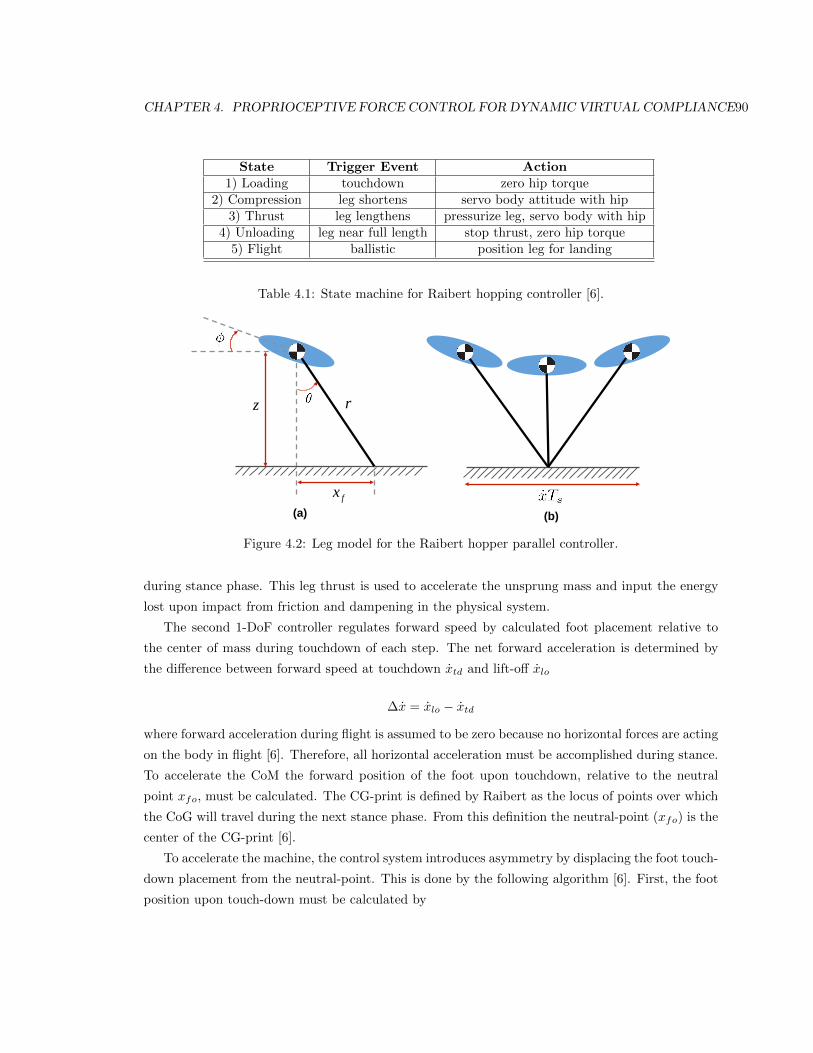
CHAPTER 4. PROPRIOCEPTIVE FORCE CONTROL FORDYNAMIC VIRTUAL COMPLIANCE90
State Trigger Event Action1) Loading touchdown zero hip torque
2) Compression leg shortens servo body attitude with hip3) Thrust leg lengthens pressurize leg, servo body with hip
4) Unloading leg near full length stop thrust, zero hip torque5) Flight ballistic position leg for landing
Table 4.1: State machine for Raibert hopping controller [6].
x f
rz
(a) (b)
Figure 4.2: Leg model for the Raibert hopper parallel controller.
during stance phase. This leg thrust is used to accelerate the unsprung mass and input the energy
lost upon impact from friction and dampening in the physical system.
The second 1-DoF controller regulates forward speed by calculated foot placement relative to
the center of mass during touchdown of each step. The net forward acceleration is determined by
the difference between forward speed at touchdown xtd and lift-off xlo
∆x = xlo − xtd
where forward acceleration during flight is assumed to be zero because no horizontal forces are acting
on the body in flight [6]. Therefore, all horizontal acceleration must be accomplished during stance.
To accelerate the CoM the forward position of the foot upon touchdown, relative to the neutral
point xfo, must be calculated. The CG-print is defined by Raibert as the locus of points over which
the CoG will travel during the next stance phase. From this definition the neutral-point (xfo) is the
center of the CG-print [6].
To accelerate the machine, the control system introduces asymmetry by displacing the foot touch-
down placement from the neutral-point. This is done by the following algorithm [6]. First, the foot
position upon touch-down must be calculated by
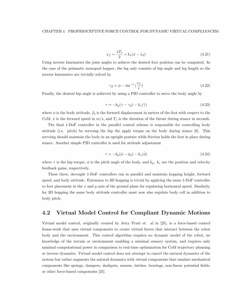
CHAPTER 4. PROPRIOCEPTIVE FORCE CONTROL FORDYNAMIC VIRTUAL COMPLIANCE91
xf =xTs2
+ kx(x− xd) (4.21)
Using inverse kinematics the joint angles to achieve the desired foot position can be computed. In
the case of the prismatic monopod hopper, the leg only consists of hip angle and leg length so the
inverse kinematics are trivially solved by
γd = φ− sin−1 (xfr
) (4.22)
Finally, the desired hip angle is achieved by using a PID controller to servo the body angle by
τ = −kp(γ − γd)− kv(γ) (4.23)
where φ is the body attitude, f0 is the forward displacement in meters of the foot with respect to the
CoM, x is the forward speed in m/s, and Ts is the duration of the thrust during stance in seconds.
The final 1-DoF controller in the parallel control scheme is responsible for controlling body
attitude (i.e. pitch) by servoing the hip the apply torque on the body during stance [6]. This
servoing should maintain the body in an upright posture while friction holds the foot in place during
stance. Another simple PID controller is used for attitude adjustment
τ = −kp(φ− φd)− kv(φ) (4.24)
where τ is the hip torque, φ is the pitch angle of the body, and kp, kv are the position and velocity
feedback gains, respectively.
These three, decouple 1-DoF controllers run in parallel and maintain hopping height, forward
speed, and body attitude. Extension to 3D hopping is trivial by applying the same 1-DoF controller
to foot placement in the x and y axis of the ground plane for regulating horizontal speed. Similarly,
for 3D hopping the same body attitude controller must now also regulate body roll in addition to
body pitch.
4.2 Virtual Model Control for Compliant Dynamic Motions
Virtual model control, originally created by Jerry Pratt et. al in [25], is a force-based control
frame-work that uses virtual components to create virtual forces that interact between the robot
body and the environment. This control algorithm requires no dynamic model of the robot, no
knowledge of the terrain or environment enabling a minimal sensory system, and requires only
minimal computational power in comparison to real-time optimization for CoM trajectory planning
or inverse dynamics. Virtual model control does not attempt to cancel the natural dynamics of the
system but rather augments the natural dynamics with virtual components that emulate mechanical
components like springs, dampers, dashpots, masses, latches, bearings, non-linear potential fields,
or other force-based components [25].

CHAPTER 4. PROPRIOCEPTIVE FORCE CONTROL FORDYNAMIC VIRTUAL COMPLIANCE92
The use of virtual model control for compliant monopod hopping allows virtual spring and damper
components to be created using high bandwidth motors with accurate proprioceptive torque sensing
to mimic the forces produced by mechanical spring and dampers.
4.2.1 Virtual Joint Compliance
Virtual joint compliance is accomplished by servoing the torque of each joint actuator to emulate the
torques that would be produced if a physical torsion spring was located in the hip joint instead
of a motor. This commanded torque (τ) at every instant is a function of the angular position error
which is the difference between the nominal virtual torsion-spring position (θ0) and the feedback
joint position (θfbk) by
τ = −ks(θ0 − θfbk)− kd(θ) (4.25)
4.2.2 Virtual Full Leg Compliance
Virtual full leg compliance is accomplished by servoing the torque of each joint actuator — using
the Jacobian transpose method — at kHz timescales to produce foot forces which would match
the force applied on the body if a physical prismatic-spring connected the hip to the foot.
Implementing virtual spring and dampers can be done by specifying a time-varying force-torque
wrench as a function of nominal foot position and foot velocity as follows.
F = [0 0 fz 0 0 0]T (4.26)
where,
fz = ks(zfbk − zcmd) + kd(zfbk − zcmd) (4.27)
where fz is the vertical component of the force torque wrench to be applied by the leg emulating a
virtual spring-damper, ks is the virtual spring stiffness [N/m], kd is the virtual dampening coefficient
[N-s/m], and z is the z-coordinate of the foot position where the subscripts zcmd and zfbk denote the
commanded and feedback positions. Typically zcmd, the commanded foot velocity in the z-direction,
is set to zero. To emulate a spring applying 3D forces the force-torque wrench can be modified as
such
F = [fx fy fz mx my mz]T (4.28)
where fx and fy are of the same form as eq. 4.27 using the corresponding position and velocity
feedback and commands xfbk, yfbk.

CHAPTER 4. PROPRIOCEPTIVE FORCE CONTROL FORDYNAMIC VIRTUAL COMPLIANCE93
fx = ks,x(xfbk − xcmd) + kd,x(xfbk − xcmd) (4.29)
fy = ks,y(yfbk − ycmd) + kd,y(yfbk − ycmd) (4.30)
Once the virtual spring force-torque wrench F is determined with any desired spring and damp-
ening coefficients (within the motors capabilities) the joint torques (τ) needed to produce this virtual
force at any instant in time can be calculated using the Jacobian transpose of the leg (JT ) by
τ = JTF (4.31)
To test the virtual model control the leg will jump and then land using virtual compliance
to absorb the impulse and a damper to prevent oscillations. In future experiments it would be
interesting to augment the system with a mechanical parallel spring combined with the virtual
compliance to achieve both variable stiffness by using the virtual compliance to modulate the stiffness
of the mechanical spring in real time while taking advantage of the fact that a mechanical spring can
store and transmit energy for higher efficiency whereas virtual compliance alone cannot do so. The
combined mechanical and virtual compliance also enables the leg to preload the mechanical spring
which can then be used to induce more explosive jumping maneuvers and agile motions.
4.2.3 Simulation Model
A simulation of the leg was created in MATLAB’s SimMechanics physics engine. A model of the
3-RSR leg was created, shown in Fig. 4.3, was used to simulate virtual model control for a 1-DoF
hopping monopod.
The simulation dropped the leg from an initial height of 0.5 m and various virtual spring and
damper coefficients were tested to determine optimal virtual component parameters for landing
while absorbing energy and minimizing oscillations (i.e. bouncing). To decrease oscillations the
dampening coefficient was increased and to absorb the impact of landing the spring stiffness was
decreased until desired performance was achieved.
4.2.4 Experimental Validation
Control for Virtual Spring-Damper Leg
The control architecture for the 1-DoF hopping controller which uses virtual model control to vir-
tually emulate a mechanical spring/damper is shown in Fig. 4.5. This controller allows the leg to
compliantly absorb the impact during touchdown/landing, while providing large leg thrust forces
for exerting large amounts of energy required for high jumping. The controller has a Flight and
Stance phase of which the stance phase is composed of two sub-states: 1) stance and 2) jump.

CHAPTER 4. PROPRIOCEPTIVE FORCE CONTROL FORDYNAMIC VIRTUAL COMPLIANCE94
Impedance Control Using Continuous Gain Scheduling
To achieve high-fidelity virtual compliance a modified impedance controller which modulates position
gains rather than joint position to generate a desired torque trajectory was implemented. The
components of the impedance control scheme are shown within the dotted box in the controller flow
diagram in Fig. 4.5. Once a virtual spring-damper foot force is determined at a given instance
in time, the Jacobian is used to transform that virtual spring-damper foot force into joint torques
at the 3-RSR’s 3 hip joints. These 3 joint torques becomes the desired torque command at the
current time step. The desired joint torques τ are then fed, along with the joint position error
(poserr = posfbk−poscmd), to the impedance controller. The impedance controller then interpolates
between the calibrated family of position error vs torque curves for various position gains (shown
in Fig. 4.4) to determine the continuous gain value which will generate the desired torque at the
current position error. This gain value is modulated and assigned at a frequency of 1 kHz1 which
enables the leg to mimic the response of a virtual spring damper at a very high bandwidth.
The controller then operates in a finite state machine as follows. While the leg is in stance and a
jump is to be initiated from rest the leg is put into a crouched position and the virtual stiffness of the
leg is set to be 1000 N/m. The jump is then initiated when the foot position is commanded to be fully
extended. The impedance controller delivers around 6 N-m for approximately 80-100 ms while the
virtual spring in the leg propels the robot upward in a dynamic and explosive jump. The controller
then enters the flight phase of the finite state machine and immediately lowers the virtual leg stiffness
to prepare for landing compliantly. The landing leg stiffness was tuned for the best performance as
a stiffness that was too soft resulted in the foot position error upon landing being large and if the
1modulated at 1 kHz in the high-level controller but the system bandwidth is around 200-250 Hz as shown in Fig.4.6
Figure 4.3: MATLAB SimMechanics model of the 3-DoF, 3-RSR leg being simulated for 1-DoFhopping and compliant landing.
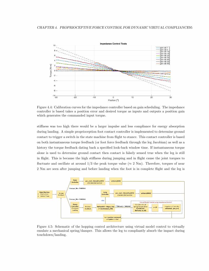
CHAPTER 4. PROPRIOCEPTIVE FORCE CONTROL FORDYNAMIC VIRTUAL COMPLIANCE95
Figure 4.4: Calibration curves for the impedance controller based on gain scheduling. The impedancecontroller is based takes a position error and desired torque as inputs and outputs a position gainwhich generates the commanded input torque.
stiffness was too high there would be a larger impulse and less compliance for energy absorption
during landing. A simple proprioception foot contact controller is implemented to determine ground
contact to trigger a switch in the state machine from flight to stance. This contact controller is based
on both instantaneous torque feedback (or foot force feedback through the leg Jacobian) as well as a
history the torque feedback dating back a specified look-back window time. If instantaneous torque
alone is used to determine ground contact then contact is falsely sensed true when the leg is still
in flight. This is because the high stiffness during jumping and in flight cause the joint torques to
fluctuate and oscillate at around 1/3 the peak torque value (≈ 2 Nm). Therefore, torques of near
2 Nm are seen after jumping and before landing when the foot is in complete flight and the leg is
Figure 4.5: Schematic of the hopping control architecture using virtual model control to virtuallyemulate a mechanical spring/damper. This allows the leg to compliantly absorb the impact duringtouchdown/landing.

CHAPTER 4. PROPRIOCEPTIVE FORCE CONTROL FORDYNAMIC VIRTUAL COMPLIANCE96
stabilizing from the jump impulse it just delivered. Therefore, if a torque threshold alone is applied
to determine ground contact, that threshold would have to be around 2N-m or greater. A threshold
that large significantly reduces the bandwidth of contact sensing or ’reaction time’ from which the
robot can switch its state machine from the flight controller to the stance controller. This is because
once the leg comes into contact with the ground the torque feedback only method of proprioception
will wait until the joint torques (or foot force) reach 2 Nm before triggering a switch in states. This
time could be on the order of milliseconds which is visible through experimentation. Therefore by
using the torque feedback history the contact controller can ’filter out’ any false positive contacts
that occur while in flight because those torque peaks of 2 Nm only last temporarily and switch signs
whereas torque does not switch sign upon initial ground contact until the rebound occurs (i.e. when
the body begins to move upward again after landing). This second method also decreases contact
sensing bandwidth because it requires looking back at a short window of time but can be tuned to
detect contact faster and more accurately than the first method. A contact controller can be avoided
all together by fine tuning the landing stiffness (position gain of the foot) such that foot position
is adequate without compromising landing compliance significantly. In this case the state machine
is triggered by a designated admissible timer which always underestimates the time it takes for the
robot to land after a jump. From testing, a timer value of 0.2 seconds seems to always work.
Once a land occurs and the state machine is switch to stance phase, the virtual model impedance
controller operates and modulates hip torques to produce effective whole leg compliance which
mimics a mechanical spring between the hip and the foot. This controller operates until the foot
position or virtual spring is compressed passed a certain threshold in which the jump controller is
called in the case of continuous hopping. This allows the energy transfer of the landing rebound
to aid the motors in generating leg lift-off thrust to jump again. Once a jump occurs, the produce
repeats to produce cyclic hopping with a stable apex hopping height.
4.2.5 Virtual Compliance Experiments
Using the continuous gain scheduling impedance controller, precise torques could be generated at the
hip joint at over 200 Hz enabling high fidelity virtual model control. Numerous tests were conducted
using various virtual spring and dampers. Virtual compliance was tested at the joint level as joint
compliance — emulating the use of physical torsion springs at hip — and as full leg compliance —
emulating the use of a physical spring-damper connecting the hip to the foot. These two virtual
compliance approaches are shown in Fig. 4.8. The results for three such tests using virtual joint and
full leg compliance are shown in Fig. 4.12. The two top rows correspond to torsional joint springs
with stiffness of 18 and 36 Nm/rad, respectively, while the bottom plot has a full leg virtual stiffness
of 250 N/m and dampening of 10 N-s/m. The full leg compliance uses a rectified virtual linear spring-
damper in which the spring can only exert forces in the negative z-direction. This rectified spring
is used to achieve shorter settling times and lower percent overshoot which is normally handled by

CHAPTER 4. PROPRIOCEPTIVE FORCE CONTROL FORDYNAMIC VIRTUAL COMPLIANCE97
Figure 4.6: Experimental results using impedance controller based on continuous gain scheduling.The position error increases linearly with time but the commanded torque trajectory is non-linear(sinusoidal). Any arbitrary torque trajectory can be chosen; the continuous gain scheduler willmodulate the gain based on the desired torque and the current position error. The torque trajectoryis followed within 10% error by the direct-drive actuator at a bandwidth greater than 200 Hz.
Figure 4.7: High jump experiments with the GOAT leg delivering 20.11 J of energy to producea maximum jump height of 82 cm which is more than double the body height. For Full video:https://www.youtube.com/watch?v=n319xVomJTQ

CHAPTER 4. PROPRIOCEPTIVE FORCE CONTROL FORDYNAMIC VIRTUAL COMPLIANCE98
Robot Legs DoF Leg Mass Motor Gear Max Vertical Energy
# # Length [m] [kg] Mass % Ratio Jump Height [m] Delivered [J]
GOAT 1 3 0.26 2.5 48 n/a 0.82 20.11
MIT Cheetah 4 3 0.275 33 24 5.8 0.5 161.9
Minitaur 4 2 0.2 5.0 40 n/a 0.48 23.5
XRL 6 1 0.2 8 11 23 0.425 33.3
Delta Hopper 1 3 0.2 2.0 38 n/a 0.35 6.9
StarlETH 4 3 0.2 23 16 100 0.32 72.2
HRP3La-JSK 2 6 0.6 54 9.2 ?? 0.27 143
ATRIAS 2 3 0.42 60 11 50 0.11 64.7
Table 4.2: Agile Performance Comparison in Dynamic Legged Robots. The bulk of the data fromthis table has been tabulated and presented originally by Kenneally et. al in [12]. The performancespecifications of GOAT are added to Kenneally’s table for purpose of comparison to other dynamiclegged machines. We introduce a slightly different metric however for vertical agility which is justthe max jumping height of the robot’s body and the energy delivered to the body during the jump.DoF is the degrees of freedom per leg.
increasing the virtual damper force. However, feedback during experiments yielded a noisy derivative
term in the virtual damper force kd(zfbk − zcmd). Therefore, the rectified spring has a similar effect
on performance as increasing the dampening would but it allows for relatively low virtual dampening
coefficients since high coefficients amplify the noise which results in leg jitter. The response for the
whole leg compliance with rectified spring-damper force is shown to be ideal as the settling time is
the shortest at 0.17 seconds compared to the settling times of the joint compliance (¿ 2 seconds).
In these tests the two performance results desired were minimized settling time and minimized
overshoot2
Vertical Agility Experiments
Several high jump experiments were conducted to determine the maximum jumping height for the
leg. Within the preliminary tests a maximum jumping height of 82 cm was attained. The robot
was able to land compliantly from all jump heights indicating that joint torques required for landing
were not the limiting factor. The experimental energy delivered Ed during the highest jump was
found to be 20.11 J.
Ed = mghpeak = (2.5 kg)(9.81m
s2)(0.82 m) = 20.11J (4.32)
Although the Table 4.2 shows that the GOAT leg is capable of jumping higher than any other
electrically actuated legged robot, this comparison is not currently fair as the rest of the robots have
on board power and electronics which is currently off-board for GOAT. The added weight of the
2where overshoot would lead to the leg hopping once it rebounded off the ground and long settling times wouldmean the robot oscillated for longer than desired before reaching steady state.

CHAPTER 4. PROPRIOCEPTIVE FORCE CONTROL FORDYNAMIC VIRTUAL COMPLIANCE99
Figure 4.8: Experiments were conducted to compare (from left to right) 1) physical joint complianceusing mechanical torsion springs in each of the three hip joints without any motors, 2) virtual jointcompliance where motors are used to emulate torsion springs of various stiffness in the hip (nophysical springs), and 3) virtual full leg compliance where motors are used to emulate the forces ofa spring-damper connecting the hip to the foot (no physical springs). Virtual component placementis shown in blue.
Figure 4.9: Experiments using 3 different virtual spring stiffness’ and dampening coefficients andobserving the response upon landing. The top two plots have virtual joint compliance with stiffnessof 18 and 36 Nm/rad while the bottom plot has a full leg virtual rectified spring stiffness of 250 N/mand dampening of 10 N-s/m. The response for the whole leg compliance is ideal with the shownparameters.

CHAPTER 4. PROPRIOCEPTIVE FORCE CONTROL FORDYNAMIC VIRTUAL COMPLIANCE100
battery and electronics is expected to be around 0.5 to 1 kg.
4.2.6 Proprioceptive Foot Force Sensing
To determine the accuracy of the proprioceptive foot force sensing capabilities the leg was com-
manded to jump a certain height and then land while the torque at each of the motors was calculated
by directly measuring current draw (τm = kt ∗ i). The motor torques τfbk were then used with the
inverse leg Jacobian transpose (JT )−1 in eq. 4.33 to determine the foot force which should have
been produced (assuming no friction in the mechanism).
Fp = (JT )−1τfbk (4.33)
This proprioceptive foot force Fp was then compared to a 6-axis force plate at the foot for ground
truth. The max error in foot force sensing through proprioceptive current sensing was determined
to be 36%. The average error however is much lower at 16% which gives an indication of the
quality of the force transparency of the actuator and leg mechanism combined. These initial tests
were conducted on a 1-DOF vertical jumping test rig and results from two such tests are shown in
Figs. 4.10-4.11. The oscillations after the immediate jump are due to high position gains from the
impedance controller when the leg is in flight (i.e. the leg is not in contact with the force plate).
4.2.7 1-DoF Vertical Hopping
Hopping tests were also included in the preliminary experiments. The hopping control framework
described in Fig. 4.5 is used to deliver leg thrusts during take-off and operate using a continuous gain
scheduling impedance controller during landing to absorb impacts smoothly using virtual compliance.
The data from a sample of 10 seconds of 30 cm hopping at 1.5 Hz on a 1-DoF test rig is shown in
Fig. 4.12. The leg was commanded to have a virtual whole leg compliance emulating a rectified
prismatic spring with a stiffness of 375 N/m and dampening of 0 N-s/m.

CHAPTER 4. PROPRIOCEPTIVE FORCE CONTROL FORDYNAMIC VIRTUAL COMPLIANCE101
Figure 4.10: To determine the accuracy of the proprioceptive sensing of foot forces through motorcurrent the actuator torque feedback is plugged into eq 4.33 to calculate the foot force. Thiscalculated proprioceptive foot force is then compared to the ground truth from the 6-axis force-torqueplate. The data shown here is from a jump/land experiment with virtual whole leg compliance withstiffness of 400 N/m and dampening of 15 N-s/m.

CHAPTER 4. PROPRIOCEPTIVE FORCE CONTROL FORDYNAMIC VIRTUAL COMPLIANCE102
Figure 4.11: Data from a second test showing proprioceptive foot force sensing accuracy during ajump/land experiment.
Figure 4.12: GOAT leg performing continuous 30 cm hopping at 1.5 Hz on a 1-DoF test rig.
Chapter 5
Conclusion and Future Work
At the time of this writing the GOAT leg has just been conceived and has only under gone a few
weeks of preliminary testing. There is still plenty of analysis and further experimentation that can
and should be done to further characterize the leg’s current performance and the magnitude of its
potential future performance. The first order of work that must be done is to finish the custom
electronics and motor controllers so that all the electronics and power can be mounted on-board the
robot. Once that is done a more fair maximum jumping height can be attained and GOAT can be
compared more closely to other, untethered, agile jumping legged robots. Energy tests measuring
the cost of transport and the efficiency of the entire leg system in converting electrical energy
into gravitational potential energy during a jump would also be interested for comparison purposes
between direct-drive and quasi-direct drive actuation. It is expected that quasi-direct-drive will
consume much less energy because the motors will not be operating in their most inefficient regime
(low speed high torque) where Joule heating losses dominate energy consumption. These measures
will also be important to understand where GOAT falls with respect to efficiency as compared to
other robots with high efficiency like the MIT Cheetah.
Once the custom electronics are developed, the leg will ideally be removed from the 1-DoF test rig
and tested in fully unconstrained 3D space (6-DoF) initially using simple Raibert style controllers.
This will allow for true testing of the leg’s robustness to 3D forces during omni-directional hopping.
Another interesting avenue for future research is augmenting the GOAT leg with a physical spring
connecting the hip to the foot. This will allow the leg to recycle energy from stride to stride in the
gait cycle by storing kinetic energy during touch-down as elastic energy and then re-delivering that
energy during take-off. The effective stiffness of the leg could still be modulated by using virtual
compliance in parallel with physical compliance to attain the benefits of both variable stiffness and
energy recycling for enhanced efficiency.
Finally, perhaps the most exciting avenue for future exploration is adapting the GOAT leg to
alternative robot morphologies like a biped or quadruped which have more stability than a monopod.
103

CHAPTER 5. CONCLUSION AND FUTURE WORK 104
This would allow for a whole host of other agility maneuvers to be created, tested, and further
explored. Because the leg is capable of delivering omni-directional force, a biped or quadruped
using the leg topology will most likely behave unlike any other legged robots or legged animals.
Instantaneous direction changes while running have the potential to create very unique mobility for
future robots that has been unseen to this point in time.
There are many other potential paths for future research with this leg but at the current time the
only certainty is that more testing and experimentation in 3D needs to be done to truly determine
what the full potential of the GOAT leg is and if it has real-world utility.

Bibliography
[1] National Geographic, Mountain Goat. [Online]. Available:
http://animals.nationalgeographic.com/animals/mammals/mountain-goat/
[2] Boston Dynamics [Online]. Available: bostondynamics.com
[3] Atlas, The Next Generation. Boston Dynamics. https://www.youtube.com/watch?v=rVlhMGQgDkY
[4] Introducing SpotMini. Boston Dynamics. https://www.youtube.com/watch?v=tf7IEVTDjng
[5] Atlas, The Next Generation. Boston Dynamics. https://www.youtube.com/watch?v=rVlhMGQgDkY
[6] M. Raibert, Legged robots that balance. MIT Press Cambridge, MA, 1986.
[7] M. Raibert, K. Blankespoor, G. Nelson, and R. Playter, Bigdog, the rough- terrain quadruped
robot, Proceedings of the 17th International Federation of Automation Control. April 2008.
[8] C. Semini. ”HyQ - Design and Development of a Hydraulically Actuated Quadruped Robot.”
Doctoral Thesis, Italian Institute of Technology, April 2010.
[9] S. Seok, A. Wang, D. Otten, and S. Kim, Actuator design for high force proprioceptive control
in fast legged locomotion, 2012 IEEE/RSJ International Conference on Intelligent Robots and
Systems, 2012.
[10] C. Hubicki, J. Grimes, M. Jones, D. Renjewski, A. Sprowitz, A. Abate, And J. Hurst. ”ATRIAS:
Design and Validation of a Tether-free 3D-capable Spring-Mass Bipedal Robot.” The Interna-
tional Journal of Robotics Research. June 10, 2016.
[11] M. Hutter. ”StarlETH & Co. Design and Control of Legged Robots with Compliant Actuation.”
Doctoral Thesis, ETH, 2013.
[12] G. Kenneally, A. De, D. Koditschek. ”Design Principles for a Family of Direct-Drive Legged
Robots.” IEEE ROBOTICS AND AUTOMATION LETTERS, VOL. 1, NO. 2, JULY 2016.
105

BIBLIOGRAPHY 106
[13] K. Galloway, G. Haynes, B. Ilhan, A. Johnson, R. Knopf, G. Lynch, B. Plotnick, M. White,
and D. Koditschek. ”X-RHex: A Highly Mobile Hexapedal Robot for Sensorimotor Tasks.”
[14] G. C. Haynes, J. Pusey, R. Knopf, A. M. Johnson, and D. E. Koditschek, Laboratory on legs: an
architecture for adjustable morphology with legged robots, in Unmanned Systems Technology
XIV, R. E. Karlsen, D. W. Gage, C. M. Shoemaker, and G. R. Gerhart, Eds., vol. 8387. SPIE,
2012, p. 83870W.
[15] W. Bosworth, S. Kim, N. Hogan. ”The MIT Super Mini Cheetah: A small, low-cost quadrupedal
robot for dynamic locomotion.” IEEE, SSRR. West Lafayette, Indiana, 2015.
[16] ”Google owned Schaft unveils new bipedal robot.” https://www.youtube.com/watch?v=iyZE0psQsX0
[17] W. Townsend, ”The Effect of Transmission Design on Force-Controlled Manipulator Perfor-
mance.” Doctoral Thesis, Massachusetts Institute of Technology, April 1988.
[18] W. Townsend, K. Salisbury. ”Mechanical bandwidth as a guideline to high-performance manip-
ulator design.” IEEE International Conference on Robotics and Automation, 1989.
[19] H.B. Brown, G. Zeglin. ”The Bow Leg Hooping Robot.” Proceedings. 1998 IEEE International
Conference on Robotics and Automation, 1998.
[20] B. Zeglin. ”The Bow Legged Hopping Robot” Doctoral Thesis, Carnegie Mellon University,
1999.
[21] J. Hurst. ”The Role and Implementation of Compliance in Legged Locomotion.” Doctoral The-
sis, Carnegie Mellon, 2008.
[22] K. Galloway. ”Passive Variable Compliance for Dynamic Legged Robots.” Doctoral Thesis,
University of Pennsylvania, 2010.
[23] S. Kalouche, D. Rollinson, H. Choset. ”Modularity for Maximum Mobility and Manipulation:
Control of a Reconfigurable Legged Robot with Series-Elastic Actuators.” IEEE International
Symposium on Safety, Security, and Rescue Robotics (SSRR), 2015, 1-8.
[24] D. Rollinson. ”Control and Design of Snake Robots.” Doctoral Thesis, Carnegie Mellon Uni-
versity, 2014.
[25] J. Pratt, C.M. Chew, A. Torres, P. Dilworth, G. Pratt. ” Virtual Model Control: An Intuitive
Approach for Bipedal Locomotion.” The International Journal of Robotics Research Vol. 20,
No. 2, February 2001, pp. 129-143.
[26] H. Asada and K. Youcef-Toumi, Direct-drive robots: theory and practice. MIT press, 1987.

BIBLIOGRAPHY 107
[27] M. Murphy, A. Saunders, C. Moreira, A. Rizzi, and M. Raibert, ”The LittleDog
Robot,”International Journal of Robotics Research, 2010.
[28] Sand Flea Jumping Robot. Boston Dynamics. https://www.youtube.com/watch?v=6b4ZZQkcNEo
[29] J. M. Duperret, G. D. Kenneally, J. L. Pusey, and D. E. Koditschek. ”Towards a Comparative
Measure of Legged Agility.” Experimental Robotics: The 14th International Symposium on
Experimental Robotics, 2016.
[30] S. Seok, A. Wang, M. Chuah, D. Hyun, J. Lee, D. Otten, J. Lang, Fellow, IEEE, and S. Kim
Design Principles for Energy-Efficient Legged Locomotion and Implementation on the MIT
Cheetah Robot.” IEEE/ASME Transactions on Mechatronics, 2015.
[31] H. Park, S. Kim. ”The MIT Cheetah, an Electrically-Powered Quadrupedal Robot for High-
speed Running.” Journal of the Robotics Society of Japan, Vol. 32 No. 4, pp.323 328, 2014.
[32] M. Woodward, M. Sitti. ”Design of a Miniature Integrated Multi-Modal Jumping and Gliding
Robot.” 2011 IEEE/RSJ International Conference on Intelligent Robots and Systems. 2011 SF,
CA.
[33] T. Tanaka, S. Hirose. ”Development of Leg-Wheel Hybrid Quadruped ”AirHopper” Design of
Powerful Light-weight Leg with Wheel.” 2008 IEEE/RSJ International Conference on Intelligent
Robots and Systems. 2008, Nice, France.
[34] B. Wilcox. ”ATHLETE: A Cargo-Handling Vehicle for Solar System Exploration” Aerospace
Conference, 2011 IEEE.
[35] M. Piccoli, S. Revzen, M. Yim, ” SEAL Pack Versatile, Portable, and Rapidly Deployable SEa,
Air, and Land vehicle.” 2013 IEEE International Symposium on Safety, Security, and Rescue
Robotics.
[36] S. Latscha, M. Kofron, A. Stroffolino, L. Davis, G. Merritt, M. Piccoli, M. Yim. ”Design of
a Hybrid Exploration Robot for Air and Land Deployment (H.E.R.A.L.D) for Urban Search
and Rescue Applications. 2014 IEEE/RSJ International Conference on Intelligent Robots and
Systems (IROS 2014) September 14-18, 2014, Chicago, IL, USA
[37] J. Whitney, T. Chen, J. Mars, and J. Hodgins. ”A Hybrid Hydrostatic Transmission and Human-
Safe Haptic Telepresence Robot.” Disney Research, 2016.
[38] J. McKenzie. ”Design of Robotic Quadruped Legs.” Masters Dissertation. MIT, 2012.

BIBLIOGRAPHY 108
[39] A. Tsiokanosa, E. Kellisb, A. Jamurtasa, and S. Kellisc, Passive bipedal running, The relation-
ship between jumping performance and isokinetic strength of hip and knee extensors and ankle
plantar flexors, vol. 10, pp. 107115, 2002.
[40] L. D. Maes, M. Herbin, R. Hackert, V. L. Bels, and A. Abourachid, Steady locomotion in
dogs: temporal and associated spatial coordination patterns and the effect of speed, Journal of
Experimental Biology, vol. 211, no. 1, pp. 138149, 2008.
[41] C. Semini et al., ”Additive manufacturing for agile legged robots with hydraulic actuation,”
Advanced Robotics (ICAR), 2015 International Conference on, Istanbul, 2015, pp. 123-129.
[42] E. Ackerman. ”What Boston Dynamics is Working On Next.” [Online]. Available:
http://spectrum.ieee.org/automaton/robotics/humanoids/what-boston-dynamics-is-working-
on-next
[43] G. Kenneally, D. Koditschek. ”Leg Design for Energy Management in an Electromechanical
Robot.” 2015 International Conference on Intelligent Robots and Systems, September, 2015.
[44] J. Grimes. ”ATRIAS 1.0 & 2.0 - Enabling Agile Biped Locomotion with a Template-Driven
Approach to Robot Design.” Masters Thesis, Oregon State University, 2013.
[45] Wikipedia. ”Specific Strength.” [Online]. Available: https://en.wikipedia.org/wiki/Specific˙strength
[46] A. Hughes. ”Electric Motors and Drives: Fundamentals, Types and Applications.” ISBN:
9780080522043, 2005.
[47] S. Colton. ”Design and Prototyping Methods for Brush-less Motors and Motor Control.” Mas-
ters Thesis, MIT, 2010.
[48] J. Urata, T. Hirose, Y. Namiki, Y. Nakanishi, I. Mizuuchi and M. Inaba. ”Thermal Control of
Electrical Motors for High-Power Humanoid Robots.” 2008 IEEE/RSJ International Conference
on Intelligent Robots and Systems. France, 2008.
[49] J. Urata, Y. Nakanishi, K. Okada, and M. Inaba, Design of high torque and high speed leg
module for high power humanoid, in Intelligent Robots and Systems (IROS), 2010 IEEE/RSJ
International Conference on. IEEE, 2010, pp. 4497 4502.
[50] ”Maxon DC motor Permanent magnet DC motor with coreless winding.” Maxon Academy,
maxonmotorusa.com, Nov, 16, 2015.
[51] S. Kim. ”MIT Cheetah - New Design Paradigm Shift Toward Mobiles Robots.” [Online]. Avail-
able: https://www.youtube.com/watch?v=R0dgELUeBTU

BIBLIOGRAPHY 109
[52] G. Wyeth. ”Control Issues for Velocity Sourced Series Elastic Actuators.” Proceedings of the
Australasian Conference on Robotics and Automation 2006.
[53] A. Schepelmann, M. Taylor, H. Geyer. ”Development of a Testbed for Robotic Neuromuscular
Controllers,” Robotics Systems and Science, 2008.
[54] M. Piccoli and M. Yim, Cogging torque ripple minimization via position based characterization,
in Proceedings of Robotics: Science and Systems, 2014.
[55] S. Ford, D. Rollinson, A. Willig, and H. Choset. ”Online Calibration of a Compact Series Elastic
Actuator.” IEEE ACC, Portland, OR, 2014.
[56] Field Oriented Control (FOC) Made Ultra Simple. [Online]. Available:
http://www.roboteq.com/index.php/support/microbasic-reference/100-applications/how-
to/359-field-oriented-control-foc-made-ultra-simple.
[57] WetSavannaAnimal aka Rod Vance (http://physics.stackexchange.com/users/26076/wetsavannaanimal-
aka-rod-vance), Is squared motor gearbox ratio proportional to inertia ratio?, URL (version:
2013-08-08): http://physics.stackexchange.com/q/73543
[58] G. Pratt, M. Williamson. ”Series elastic actuators.” Intelligent Robots and Systems 95.’Hu-
man Robot Interaction and Cooperative Robots’, Proceedings. 1995 IEEE/RSJ International
Conference on. Vol. 1. IEEE, 1995.
[59] N. Paine. ”High-Performance Series Elastic Actuation.” Doctoral Thesis, University of Texas,
2014.
[60] H. Horn, D. Wood, K Korane. ”Planetary gears A review of basic design criteria and new op-
tions for sizing.” [Online]. Available: http://machinedesign.com/mechanical-drives/planetary-
gears-review-basic-design-criteria-and-new-options-sizing
[61] R. Blickhan. ”The Spring-Mass Model for Running and Hopping.” J. Biomechanics Vol. 22, No
11/12, pp. 1217-1227, 1989.
[62] H. Geyer, A. Seyfarth, R. Blickhan. ”Compliant leg behaviour explains basic dynamics of walk-
ing and running.” Proc. R. Soc. B (2006) 273, 28612867 doi:10.1098/rspb.2006.3637 Published
online 11 August 2006.
[63] Blickhan R., and Full R. Similarity in multilegged locomotion: bouncing like a monopode.
Journal of Comp Phys A 173.5 (1993): 509-517.
[64] D. Ferris, M. Louie, C. Farley. ”Running in the real world: adjusting leg stiffness for different
surfaces.” Proc Biol Sci. 1998 Jun 7; 265(1400): 989994.

BIBLIOGRAPHY 110
[65] . M. Murray, Z. Li, S. S. Sastry, and S. S. Sastry, A Mathematical Introduction to Robotic
Manipulation. Boca Raton, FL, USA: CRC Press, 1994.
[66] McMaster-Carr. [Online]. Available: www.mcmaster.com
[67] The Engineering Toolbox: Metal and Alloy Density. [Online]. Available:
http://www.engineeringtoolbox.com/metal-alloys-densities-d˙50.html
[68] Microsemi. ”Park, Inverse Park and Clarke, Inverse Clarke Transformations MSS Software
Implementation User Guide.” [Online]. Available: http://www.microsemi.com/document-
portal/doc˙view/132799-park-inverse-park-and-clarke-inverse-clarke-transformations-mss-
software-implementation-user-guide
[69] M. Zieserl. ”Using Magnetic Sensor ICs In Highly Magnetic Environments.” Online: Available
sensorsmag.com, September 2015.
[70] H., Neville. Impedance control: An approach to manipulation. American Control Conference,
1984. IEEE, 1984.
[71] . D. Maes, M. Herbin, R. Hackert, V. L. Bels, and A. Abourachid, Steady locomotion in
dogs: temporal and associated spatial coordination patterns and the effect of speed, Journal of
Experimental Biology, vol. 211, no. 1, pp. 138149, 2008.
[72] A. De, D. Koditschek. ”The Penn Jerboa: A Platform for Exploring Parallel Composition of
Templates.” Technical Report, University of Pennsylvania, 2014.
[73] M. Hutter, C. Gehring, M. H. Pflinger, M. Blosch, and R. Siegwart, Fellow, IEEE. ”Toward
Combining Speed, Efficiency, Versatility, and Robustness in an Autonomous Quadruped.” IEEE
TRANSACTIONS ON ROBOTICS, VOL. 30, NO. 6, DECEMBER 2014 1427.