design, fabrication, and testing of a new small wind ... · pdf filedesign, fabrication, and...
TRANSCRIPT

Design, Fabrication, and Testing of a New Small Wind Turbine Blade
by
Qiyue Song
A Thesis
presented to
The University of Guelph
In partial fulfilment of requirements
for the degree of
Master of Applied Science
in
Engineering
Guelph, Ontario, Canada
© Qiyue Song, April, 2012
ABSTRACT
DESIGN, FABRICATION, AND TESTING OF A SMALL WIND TURBINE BLADE
Qiyue Song Advisor:
University of Guelph, 2012 Professor W. D. Lubitz
A small wind turbine blade was designed, fabricated and tested in this study. The power
performance of small horizontal axis wind turbines was simulated in detail using modified blade
element momentum methods (BEM). Various factors such as tip loss, drag coefficient, and wake
were considered. The simulation was validated by experimental data collected from a small wind
turbine Bergey XL 1.0. A new blade was designed for the Bergey XL 1.0 after comparing three
types of aerodynamic blade structures and their related performance, and then the detailed blade
structure was determined. The performance of the new rotor at different additional pitch angles
was simulated and compared with the original Bergey XL 1.0 rotor. To fabricate prototypes of the
new blades, a resin transfer moulding (RTM) system was designed and built. Three blades were
fabricated successfully and installed on the hub of an existing Bergey XL 1.0. In a vehicle-based
test system, the new blades were tested at the original designed pitch angle, plus at additional 5°
and 9° pitch angles. The +5° rotor reached maximum power of 1889 W at wind velocity 13.6 m/s.
The +9° rotor performed over a wider wind velocity range and output slightly lower power than
the original Bergey XL 1.0. The new blades have better aerodynamic performance than original
Bergey XL 1.0.

iii
ACKNOWLEDGEMENTS
I would like to express my sincere gratitude to my advisor, Dr. William David Lubitz for offering
me the opportunity to study and pursue a Master’s degree in Canada, and for valuable suggestions
not only on technology itself but also on culture and customs. I would like to thank my committee
member, Dr. Manjusri Misra, for her strong support and excellent advice on my research. Also
I’d like to thank Dr. Harekrishna Deka at the BDDC, and technical staff members Ken Graham
and Steve Wilson for their help and cooperation.
I appreciated very much the TA experiences that Dr. Funtahun M. Defersha and Dr. Marwan
Hassan provided me, and I learned much more knowledge than just the courses. I also should say
thanks to the Ontario Ministry of Agriculture and Rural Affairs (OMAFRA) New Directions
Research Program and Dr. Warren Stiver, the National Sciences and Engineering Research
Council (NSERC) Chair in Environmental Design Engineering at the University of Guelph, for
their financial support.
Thanks to my office mates, Bryan Ho-Yan, Joel Citulski, Rajendra Sapkota and Murray Lyons. I
will not forget their encouragement and counsel. Finally, thanks to everyone else that I did not
mention but helped me, even just several inspirited words.

iv
Table of contents
Chapter 1. Introduction............................................................................................................ 1
1.1. Problems and significances of small wind turbines ........................................................ 1
1.2. Objectives and scope of this study ................................................................................. 3
1.3. Contribution of this study ............................................................................................... 4
Chapter 2. Literature review .................................................................................................... 5
2.1. Composition of a small wind turbine ............................................................................. 5
2.1.1 Rotor ............................................................................................................................... 6
2.1.2 Generator ........................................................................................................................ 6
2.1.3 Nacelle............................................................................................................................ 7
2.1.4 Tail assembly ................................................................................................................. 7
2.1.5 Controller ....................................................................................................................... 8
2.2. Materials for small wind turbine blade ........................................................................... 8
2.2.1 Metal .............................................................................................................................. 9
2.2.2 Glass and carbon fibre composites ................................................................................. 9
2.2.3 Wood and bamboo ....................................................................................................... 10
2.2.4 Biocomposites .............................................................................................................. 11
2.3. Manufacturing of small wind turbine blades ................................................................ 12
2.4. Power curve of wind turbines ....................................................................................... 14
Chapter 3. Aerodynamics of horizontal axis small wind turbines ......................................... 16
3.1. Momentum theory ........................................................................................................ 16
3.1.1 Betz Limit..................................................................................................................... 16
3.1.2 Wake rotation ............................................................................................................... 18
3.2. Blade element theory .................................................................................................... 19
3.2.1 Airfoil ........................................................................................................................... 19

v
3.2.2 Blade element analysis ................................................................................................. 20
3.3. Blade element momentum theory ................................................................................. 22
3.4. Loss factors ................................................................................................................... 23
3.5. Turbulent wake state ..................................................................................................... 24
3.5.1 Glauert method ............................................................................................................. 24
3.5.2 Wilson-Walker method ................................................................................................ 25
3.5.3 Buhl method ................................................................................................................. 25
3.5.4 The tangential induction factor .................................................................................... 26
3.6. Power coefficient .......................................................................................................... 27
3.7. Simulation methods ...................................................................................................... 27
Chapter 4. Performance simulation of Bergey XL 1.0 .......................................................... 29
4.1. Introduction .................................................................................................................. 29
4.2. Bergey XL 1.0 specifications ....................................................................................... 29
4.3. Airfoil of Bergey XL 1.0 .............................................................................................. 30
4.3.1 Geometry of Bergey airfoil .......................................................................................... 30
4.3.2 XFOIL .......................................................................................................................... 30
4.3.3 Cl and Cd of the Bergey airfoil .................................................................................... 31
4.3.4 Comparison of Cl and Cd with other researcher’s results ............................................. 32
4.3.5 Lift and drag coefficient determination ........................................................................ 35
4.3.6 Lift and drag coefficients after stall ............................................................................. 36
4.4. Power coefficient .......................................................................................................... 38
4.4.1 Factors in power coefficient calculation ...................................................................... 38
4.4.2 Flat plate theory and Viterna method ........................................................................... 40
4.4.3 Wake factor .................................................................................................................. 41
4.4.4 Comparison with others’ research ................................................................................ 42

vi
4.4.5 Local power coefficient ................................................................................................ 43
4.5. Power simulation .......................................................................................................... 44
4.6. Field performance simulation ....................................................................................... 46
4.6.1 Efficiency of Bergey XL 1.0 ........................................................................................ 46
4.6.2 Test validation of simulation code ............................................................................... 47
4.6.3 Local operating condition ............................................................................................ 48
4.7. Discussion..................................................................................................................... 52
4.8. Summary of BEM method ............................................................................................ 53
Chapter 5. New blade design ................................................................................................. 55
5.1. Design specifications .................................................................................................... 55
5.2. Airfoil selection ............................................................................................................ 56
5.3. Airfoil characteristics ................................................................................................... 59
5.4. Initial blade aerodynamic parameters ........................................................................... 60
5.5. Initial performance prediction ...................................................................................... 62
5.6. Structural design of blade ............................................................................................. 65
5.6.1 Blade elements parameters ........................................................................................... 65
5.6.2 Root design................................................................................................................... 66
5.6.3 New blade geometry .................................................................................................... 68
5.7. Predicted performance of new blade ............................................................................ 68
5.8. Performance comparisons at different pitch angle ....................................................... 70
5.8.1 Power coefficient comparison ...................................................................................... 70
5.8.2 Performance comparison between new blades and Bergey ......................................... 71
Chapter 6. Blade fabrication and RTM system ..................................................................... 74
6.1. RTM system design ...................................................................................................... 74
6.1.1 Requirements of RTM system...................................................................................... 74
vii
6.1.2 RTM system utilized at University of Guelph ............................................................. 75
6.2. RTM mould design and production .............................................................................. 78
6.2.1 Blade mould design ...................................................................................................... 78
6.2.2 Stress and displacement simulation of mould .............................................................. 79
6.2.3 Mould production ......................................................................................................... 80
6.3. Blade fabrication .......................................................................................................... 82
6.4. Discussion..................................................................................................................... 82
Chapter 7. Vehicle-based test ................................................................................................ 85
7.1. Introduction .................................................................................................................. 85
7.2. Vehicle-based test system ............................................................................................. 86
7.2.1 Test road and weather .................................................................................................. 86
7.2.2 Test equipment and sensors.......................................................................................... 86
7.2.3 Data acquisition system ................................................................................................ 89
7.2.4 Test methods and influential factors ............................................................................ 89
7.3. Measurement and uncertainty ....................................................................................... 91
7.3.1 NI USB 6210 ................................................................................................................ 91
7.3.2 Output power ................................................................................................................ 92
7.3.3 Wind velocity ............................................................................................................... 92
7.3.4 Rotor rotation speed ..................................................................................................... 94
7.3.5 Tip speed ratio .............................................................................................................. 94
7.3.6 Gross power coefficient ............................................................................................... 95
7.3.7 Uncertainty summary of variables ............................................................................... 95
7.4. Raw data analysis ......................................................................................................... 95
7.4.1 Calculated raw power data ........................................................................................... 95
7.4.2 Typical road test ........................................................................................................... 98

viii
7.4.3 Data filtering .............................................................................................................. 100
7.5. Comparison of rotors .................................................................................................. 101
7.5.1 Power curve ................................................................................................................ 101
7.5.2 Wind speed vs. rotor speed ........................................................................................ 104
7.5.3 Rotor speed vs. power ................................................................................................ 104
7.5.4 Tip speed ratio ............................................................................................................ 106
7.5.5 Power coefficients ...................................................................................................... 108
7.6. Simulation of power curve ......................................................................................... 110
7.7. Discussion................................................................................................................... 112
7.8. Summary..................................................................................................................... 113
Chapter 8. Summary and conclusions ................................................................................. 116
Chapter 9. Recommendations .............................................................................................. 118
References .................................................................................................................................... 120
Appendix A: Aerodynamic parameters of the new blade ............................................................ 130
Appendix B: Anemometer verification ........................................................................................ 131
Appendix C: Example of test data verification ............................................................................ 133
ix
List of Tables
Table 1: Specifications of Bergey XL 1.0 ..................................................................................... 29
Table 2: Summary of small wind turbines in literature ................................................................ 56
Table 3: Airfoil tested for small wind turbines (Source: Selig and McGranahan, 2004) .............. 57
Table 4: Uncertainty summary of variables ................................................................................... 95
Table 5: Uncertainty and mean of tip speed ratio ........................................................................ 106
Table 6: CP summary of three rotors ........................................................................................... 108
Table A: Detailed aerodynamic parameters of the designed blade………...………………..….130

x
List of Figures
Figure 1: A blade element sweeps out an annular ring (Source: Burton et al., 2001) ..................... 2
Figure 2: Composition of a typical small wind turbine (Adapted from Bergey, 2012) ................... 5
Figure 3: A typical power curve (Source: WindPowerProgram, 2012) ......................................... 15
Figure 4: Actuator disk model for rotor analysis (Adapted from Manwell et al., 2002) ............... 16
Figure 5: Blade geometry for analysis of wind turbine (Source: Manwell et al., 2002) ............... 21
Figure 6: Different expressions for the thrust coefficient vs. the axial induction factor (Source:
Hansen, 2008) ................................................................................................................................ 26
Figure 7: Profile of Bergey XL 1.0 ................................................................................................ 30
Figure 8: The pressure distribution along airfoil in XFOIL ........................................................... 32
Figure 9: Lift coefficient of Bergey airfoil .................................................................................... 33
Figure 10: Drag coefficient of Bergey airfoil ................................................................................ 33
Figure 11: Airfoil characteristics of Bergey XL 1.0 airfoil (Source: Martinez et al., 2006) ......... 34
Figure 12: Airfoil characteristics of Bergey XL 1.0 airfoil (Source: Seitzler and Kamisky, 2008 )
....................................................................................................................................................... 34
Figure 13: Drag polar for airfoil SH3055 (Source: Selig and McGranahan, 2004) ....................... 35
Figure 14: Measured Bergey airfoil and SH3055 airfoil .............................................................. 35
Figure 15: Extended lift coefficient versus angle of attack............................................................ 37
Figure 16: Extended drag coefficient versus angle of attack ......................................................... 38
Figure 17: Comparison of power coefficients with different factors included .............................. 39
Figure 18: Power coefficient versus tip speed ratio with two methods for post-stall point ........... 40
Figure 19: Power coefficient calculation with different wake factors ........................................... 41
Figure 20: Comparison of power coefficients................................................................................ 42
Figure 21: Local power coefficients at different sections along the blade .................................... 43
Figure 22: Simulated rotor power at different rotor speeds ........................................................... 44

xi
Figure 23: Simulated rotor power from Martinez et al. (Source: Martinez et al., 2006) ............... 45
Figure 24: Simulated power of Bergey by Nichita et al. (Source: Nichita et al., 2006). ............... 46
Figure 25: Electrical system efficiency (Source: Martinez et al., 2006) ....................................... 47
Figure 26: Original power data versus wind velocity .................................................................... 49
Figure 27: Power curves of simulation, manufacturer and binned experimental data .................. 49
Figure 28: Tip speed ratio versus wind speed from the experimental data .................................... 50
Figure 29: Angle of attack along spanwise with flat plate theory .................................................. 50
Figure 30: Angle of attack along spanwise with Viterna method .................................................. 51
Figure 31: Reynolds number along the blade at different wind speed and tip speed ratio ............ 52
Figure 32: Lift coefficients of airfoil SD 7062 .............................................................................. 59
Figure 33: Drag coefficients of airfoil SD 7062 ............................................................................ 59
Figure 34: Ratio of lift coefficient over drag coefficient for airfoil SD 7062 ................................ 60
Figure 35: Chord as a function of radius determined by the three methods .................................. 63
Figure 36: Twist as a function of radius calculated by the three methods ..................................... 64
Figure 37: Extended airfoil characteristics of SD 7062 ................................................................. 64
Figure 38: Power coefficient comparison for the new blade in 3 types of parameters and the
original Bergey blade ..................................................................................................................... 65
Figure 39: All profiles in rotor rotating coordinates system .......................................................... 67
Figure 40: Airfoils of new blade and Bergey ................................................................................. 67
Figure 41: 3D solid model of the new blade .................................................................................. 68
Figure 42: Power simulation of the new blades ............................................................................. 69
Figure 43: Local power coefficient comparison at different tip speed ratios ................................. 70
Figure 44: Comparison of power coefficients................................................................................ 71
Figure 45: Power comparison between Bergey and the new blade rotor ....................................... 72
Figure 46: Power comparison between Bergey and the new rotor at +5° pitch angle ................... 73

xii
Figure 47: Power comparison between Bergey and the new rotor at + 9° pitch angle .................. 73
Figure 48: RTM system ................................................................................................................. 76
Figure 49: The physical RTM system at the University of Guelph ............................................... 77
Figure 50: 3D mould model ........................................................................................................... 80
Figure 51: Von Mises stress of the mould .................................................................................... 81
Figure 52: Resultant displacement of the mould .......................................................................... 81
Figure 53: Aluminum mould made from CNC .............................................................................. 82
Figure 54: Three blades made from RTM system at the University of Guelph ............................. 83
Figure 55: Satellite view of surroundings at Southgate road test location in Guelph .................... 87
Figure 56: Vehicle-based wind turbine test system ....................................................................... 88
Figure 57: Wiring of sensors and data acquisition system ............................................................. 90
Figure 58: Airflow around the car (Adapted from Scibor-Rylski, 1975)....................................... 94
Figure 59: Power versus wind speed for the original Bergey blades ............................................. 96
Figure 60: Power versus wind speed for the new blades at 0° pitch angle ................................... 96
Figure 61: Power versus wind speed for the new blades at +5° pitch angle .................................. 97
Figure 62: Power versus wind speed for the new blades at + 9° pitch angle ................................. 97
Figure 63: Raw data for one round test of Bergey ......................................................................... 99
Figure 64: Raw data for one round test of the new blades at + 5° pitch angle .............................. 99
Figure 65: Raw data for one round test of the new blades at + 9° pitch angle ............................ 100
Figure 66: Power curve of Bergey blade ..................................................................................... 102
Figure 67: Power curve of the new blades at +5° pitch angle...................................................... 103
Figure 68: Power curve of the new blades at + 9° pitch angle..................................................... 103
Figure 69: Power curve comparison of three rotors ..................................................................... 104
Figure 70: Rotor speed vs. wind velocity of three rotors ............................................................. 105
Figure 71: Power vs. rotor speed for three rotors ........................................................................ 105
xiii
Figure 72: Tip speed ratio vs. wind velocity for Bergey ............................................................. 106
Figure 73: Tip speed ratio vs. wind velocity for the new blades at + 5° pitch angle ................... 107
Figure 74: Tip speed ratio vs. wind velocity for the new blades at +9° pitch angle .................... 107
Figure 75: Power coefficient vs. wind velocity for Bergey ......................................................... 109
Figure 76: Power coefficient vs. wind velocity for the new blades at + 5° pitch angle ............... 109
Figure 77: Power coefficient vs. wind velocity for the new blades at + 9° pitch angle ............... 110
Figure 78: Power curve simulation of the Bergey ....................................................................... 111
Figure 79: Power curve simulation of the new blades at + 5° pitch angle ................................... 111
Figure 80: Power curve simulation of the new blades at + 9° pitch angle ................................... 112
Figure B-1: Cup anemometer verification ……………………………………………….…… 131
Figure B-2: Ultrasonic anemometer verification ……………………………………..……….. 132
Figure C-1: Example of one round test data of Bergey with outliers……………….………… 133
Figure C-2: 3s-period pulse in raw data at 21 s .………………………………….……………134
Figure C-3: 3s-period pulse in raw data at 24 s ………………………………………….……..134

xiv
Nomenclature
a Axial induction factor
a´ Tangential induction factor
A Swept area of a wind turbine rotor
AR Aspect ratio
b Blade span
B Number of blades
c Chord
c Mean chord length
Cd Drag coefficient
Cl Lift coefficient
Cn Normal load coefficient
Ct Tangential load coefficient
CP Wind turbine power coefficient
CP, Max Maximum wind turbine power coefficient (Betz limit)
CT Thrust coefficient
CTr Local thrust coefficient
D Wind turbine rotor diameter / Drag force
dFD Incremental drag force
dFL Incremental lift force
dFN Incremental normal force
dFT Incremental tangential force
frotor Measured rotor frequency
Fhub Hub loss factor
Ftip Tip loss factor

xv
F Total loss factor of wind turbine rotor
k Classification number of terrain for cup anemometer
l Airfoil span
L Length of the flow on airfoil surface / Lift force
m Mass flow rate of air
N Section number
p Air pressure
P Wind turbine power output
Poutput Measured output power from generator
Q Angular momentum
r Radial position along a wind turbine rotor
R Wind turbine rotor radius; Resistance of resistor
Re Reynolds number
Rh Radius of hub
T Force of wind on the wind turbine (Thrust)
U Wind speed
Ucupm Measured wind speed of cup anemometer,
Urel Relative wind velocity
V Voltage
VDAQ Voltage from data acquisition system
Voutput Measured output voltage from generator
x Measured variable
xm Measured value of variable
X Coordinates of axis X
Y Coordinates of axis Y
xvi
Z Coordinates of axis Y
α Angle of attack
αstall Angle of attack at stall point
Uncertainty
xA/D Uncertainty from A/D conversion
x Uncertainty of measured variable.
x inst Uncertainty from instrument itself
ø Angle of relative wind
System efficiency of wind turbine
E Efficiency of electrical system
λ Wind turbine tip speed ratio
λh Local speed ratio at hub
λr Local speed ratio
Fluid viscosity
v Kinematic viscosity
θ Pitch angle
θp Section pitch angle
θp,0 Blade pitch angle at the tip
θT Section twist angle
ρ Fluid (air) density
σ Local solidity
ω Angular velocity of the wind
Ω Rotor rotational speed

1
Chapter 1. Introduction
1.1. Problems and significances of small wind turbines
In recent years, wind energy has drawn more attention due to the increasing prices of fossil fuels
and improving economic competitiveness of wind turbines relative to conventional generation
technologies. Today, wind energy has been developed into a mature, competitive, and virtually
pollution-free technology. Usually a typical large, utility scale wind turbine can produce 1.5 to
4.0 million kWh annually and operates 70-85% of the time (Balat, 2009). Global wind energy
production set a new record in 2011, reaching 239 GW, 3% of total electricity production
(WWEA, 2012). It is predicted that by 2020 it will increase to 10% of global electricity
production (Compositesworld, 2012).
The American Wind Energy Association (AWEA) reported in 2010 that production of small
horizontal-axis wind turbines would increase rapidly in the future due to huge demand (AWEA,
2010). For the classification of horizontal-axis wind turbines, there is no fixed standard. The
National Renewable Energy Laboratory (NREL) in US defines wind turbines whose rated power
are not greater than 100 kW (NREL, 2012), and whose diameter are no more than 19 m as small
wind turbines (Compositesworld, 2012). Clausen and Wood (2000) defined a small wind turbine
as having a maximum power output of 50 kW, and further divided small wind turbines into three
categories: micro turbines (maximum 1 kW); mid-range (larger than micro ones and smaller than
mini ones), usually 1 kW to 5 kW; and mini turbines whose power greater than 20 kW. In this
paper the small horizontal-axis wind turbines around 1 kW is the focus, which are referred to by
default as small wind turbines.
2
The technology of large wind turbines has been developed well, however, small wind turbines
need more research because of different structures and different applications from large ones
(Clausen and Wood, 2000). Evidently, power performance is the first consideration to improve.
Though Computational Fluid Dynamics (CFD) has been developing to explore aerodynamics of
wind turbines, the Blade Element Momentum (BEM) method is still applied widely for it is a
simple, immediate and effective method for small wind turbine design and performance analysis.
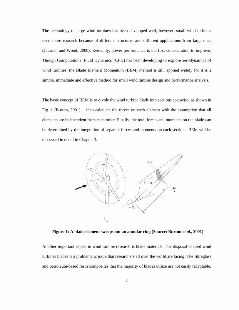
The basic concept of BEM is to divide the wind turbine blade into sections spanwise, as shown in
Fig. 1 (Burton, 2001), then calculate the forces on each element with the assumption that all
elements are independent from each other. Finally, the total forces and moments on the blade can
be determined by the integration of separate forces and moments on each section. BEM will be
discussed in detail in Chapter 3.
Figure 1: A blade element sweeps out an annular ring (Source: Burton et al., 2001)
Another important aspect in wind turbine research is blade materials. The disposal of used wind
turbines blades is a problematic issue that researchers all over the world are facing. The fibreglass
and petroleum-based resin composites that the majority of blades utilize are not easily recyclable.

3
Current methods for wind turbine blade disposal include landfill, incineration and limited
recycling (Larsen, 2011). However, obviously no disposal method is perfect. An alternative that
can mitigate some of the issues with current disposal methods is to develop “green” materials to
replace the conventional materials (Larsen, 2011).
The project Hierarchical Green Nano-Biocomposites for Light Weight and Efficient Wind
Turbines Blades was launched to explore new blade materials from bio-sources for small wind
turbines with improved power performance. The study documented in this thesis was part of this
larger project.
1.2. Objectives and scope of this study
The objective of this research project was to design, fabricate and test a new blade for a Bergey
XL 1.0 small wind turbine. To reach this goal, the following sections were completed:
Reviewed the literature related to the design of small wind turbine blades using BEM.
Surveyed modified BEM methods developed by other researchers, analyzed the
underlying assumptions, practicality and performance of these methods. Compared these
different methods using similar test cases.
Consolidated prior BEM knowledge and developed a BEM method specifically suited to
simulate the original and new blades for a small wind turbine like the Bergey XL 1.0.
Validated the simulation code of BEM method using measured field test data from a
Bergey XL 1.0; for the determination of Bergey airfoil, compared the calculation of lift
and drag coefficients from Xfoil with the calculated data of other researchers, confirming
validation of Xfoil for simulation.

4
Designed a new blade with higher or close performance to the original Bergey blade,
including airfoil selection, performance evaluation at different pitch angles, and blade
structural design in a 3 dimensional model.
Designed a set of RTM moulds for blade production; designed and constructed a simple
but effective RTM system, and produced three blades made of fibre glass and epoxy
composite.
Installed Bergey blades and new blades at 0, +5 , +9 pitch angles on Bergey hub and
tested these rotors in a vehicle-based testing system to evaluate and compare the power
performance.
Compared all test data of different rotors with each other as well as with the simulation
code.
1.3. Contribution of this study
Detailed modified BEM methods were analyzed to determine various factors’ weight for a
small wind turbine Bergey XL 1.0. This can be extended to other small wind turbine
performance analysis and prediction.
A new blade was designed based on BEM performance simulation; the RTM system was
proven to be a good method for blade building with low cost and consistent quality in
blade geometry and surface finish.
Vehicle-based testing validated that the new blade has higher aerodynamic performance
than original Bergey XL 1.0; the experimental data further proved that BEM analysis
could be accepted for performance prediction for small wind turbines when relative
factors are chosen correctly.

5
Chapter 2. Literature review
2.1. Composition of a small wind turbine
In general, all wind turbines consist of a rotor, generator and tower. However, large utility scale
turbines are more complex than small turbines. Virtually all commercial utility scale turbines
have an active yaw system to point the rotor to face the wind and a gearbox that turns the
generator at a faster rotation rate than the rotor for producing electricity efficiently (Manwell et
al., 2002). On the other hand, small turbines usually use tails or a downwind configuration to
passively point the rotor to windward, and many small wind turbines directly connect the rotor
and generator, without a gearbox (Manwell et al., 2002). Fig. 2 shows the main components of a
Bergey XL 1.0, a common small wind turbine.
Figure 2: Composition of a typical small wind turbine (Adapted from Bergey, 2012)

6
2.1.1 Rotor
The rotor is the most important component in a wind turbine, designed to capture wind energy
and convert it into rotating mechanical energy. The rotor should be strong enough to stand steady,
periodic and randomly changing loads (Manwell et al., 2002). The rotor assembly consists of
several blades joined to a common hub, a cone nose and fasteners.
The blades are critical components of the rotor, and consist of the airfoils which interact with the
wind and convert the power in the wind to mechanical power. The geometry and dimensions of
the blades are determined by the performance requirements of the wind turbine. Two fundamental
issues must be considered simultaneously in blade design process: aerodynamic performance and
structural design (Manwell et al., 2002). For example, after the overall shape of the blade is
optimized aerodynamically, it is common that the root of the blade must be redesigned to
meet structural requirements. Aerodynamically advantageous features such as sharp
trailing edges are often so difficult to build that compromises must be made so that the
blade design can be manufactured. The choice of materials and manufacturing methods
for the blades should also be considered during structural design and strength analysis.
The hub is the part which transmits all the power and loads from the blades to the main shaft.
There are three types of hubs: rigid, teetering and hinged (Manwell, et al., 2002). A rigid hub is
the simplest and most common; it supports the blades in fixed positions relative to the main shaft.
2.1.2 Generator
In all electricity generating wind turbines, a generator converts the mechanical power from the
rotating wind blades to electrical power. Induction generators and synchronous generators are
among the most common generators in large wind turbines (Burton, et al., 2001). Most small

7
wind turbines use direct drive generators, which are actually special synchronous generators with
enough poles to enable generator work well at the same speed of wind turbine rotor (Burton, et
al., 2001). Because there is no gearbox required with these generators, the reliability of the
system is generally better than when a gearbox is included. The Bergey XL 1.0 used in this study
employs a direct drive permanent magnet alternator. Permanent magnets mounted on the interior
surface of the rotating hub pass close to stationary coils mounted to the main frame. The changing
magnetic field at the coils induces three-phase alternating current that is rectified to direct current
by a rectifier in the nacelle (Bergey, 2012).
2.1.3 Nacelle
The turbine nacelle houses all the principal components of the wind turbine except the rotor.
Within the nacelle, a main frame provides the backbone of the wind turbine; the bearings
supporting the hub, generator, tail assembly and yaw bearings are all connected to it. A nacelle
cover protects these components from sunlight, rain, ice and snow. The Bergey XL 1.0 nacelle
also contains the rectifier, slip-ring assembly and tower mount.
2.1.4 Tail assembly
Most small wind turbines are pointed into the wind using a tail assembly. A tail assembly usually
consists of tail fin and tail boom, which are the primary components of the yaw system, keeping
the turbine pointed into the wind. Larger turbines generally dispense with a tail because as the
turbine size increases, the weight and loads associated with a tail become excessive. Instead, most
large turbines use an active yaw system in which geared motors point the turbine into the wind
based on the readings of wind direction sensors mounted on the nacelle.
In many small wind turbines, the tail assembly includes an auto-furling system. Furling is the
most popular mechanism in small turbines to limit rotor speed, power output and wind loads in

8
extreme winds. Furling is also used in the products of Bergey and Southwest Windpower. In the
turbines from these companies, the rotor is installed eccentrically with respect to the yaw axis (or
vertical axis). The rotor thrust produces a moment about the yaw axis. Furling occurs if the thrust
becomes too great: the rotor pivots relative to the tail fin, which is hinged where it joins the main
frame, with the effect of turning the rotor to face away from the prevailing wind direction
(Audierne et al., 2010). When wind speed is below the rated critical point, the rotor is kept
oriented to the wind; otherwise, furling will work to protect the rotor and generator.
The Bergey XL 1.0 operates normally when wind speed is less than 13m/s. However, at wind
speeds between 13 m/s and 18 m/s, the wind turbine will partially furl (turn partly out of the
wind), or furl and unfurl repeatedly. At wind speeds greater than 18 m/s, the turbine will furl
completely, meaning that the plane of the rotor disk will be aligned with the prevailing wind
direction (Bergey, 2012).
2.1.5 Controller
Controller technology for wind turbines ranges widely from dynamic control systems to
supervisory control systems and computer, which vary on different wind turbine systems. Small
wind turbines can utilize a controller to covert the variable, noisy power from the generator into a
steady direct current at an appropriate voltage for charging batteries. The Bergey XL 1.0 has an
extra electrical controller box (also called power centre) connecting the generator and battery
bank to regulate battery charging system (Bergey, 2012).
2.2. Materials for small wind turbine blade
The blades in a normally operating wind turbine rotor are continuously exposed to cyclical loads
from wind and gravity. The expected lifetime for a blade is usually 20 years for large wind
turbines, and less than 20 years for small wind turbines (Clausen and Wood, 2000). Based on

9
these conditions, Brøndsted et al. (2005) summarized that the primary requirements for blade
materials are high stiffness to ensure aerodynamic performance, low density to minimize mass
and long-fatigue cycles. In the wind turbine industry, many materials have been used for blades,
including metals, plastics, wood and composites (Manwell et al., 2002).
2.2.1 Metal
Steel is a common, relatively inexpensive material used extensively in industry, however, it is
difficult to manufacture into a complex twisted shape, and the fatigue life of steel is very poor
compared to fibreglass composites (Burton et al., 2001). While steel was used for wind turbines
blades before the 1950s, it is essentially no longer used (Manwell et al., 2002).
Another metal that has been considered for wind turbine blades is weldable aluminum. However,
its fatigue strength at 107 cycles is only 17 MPa compared with fibreglass 140 MPa and carbon
fibre 350 MPa (Burton et al., 2001). Aluminum was sometimes used for small wind turbine
blades, usually to produce non-twisted blades by protrusion (Manwell et al., 2002). However, like
steel, aluminum is little used in practice.
2.2.2 Glass and carbon fibre composites
While various materials have been applied successfully in wind turbine blades, fibreglass based
composites predominate (Veers et al., 2003). This is mostly because fibreglass is a low-cost and
high tensile strength material. It is also easily knitted and woven into desired textiles to meet
different engineering requirements (Manwell et al., 2002). Usually the fibreglass is embedded
within a plastic matrix to form a composite known as glass reinforced plastic (GRP).
Carbon fibre is also becoming more popular because it has higher modulus, lower density and
higher tensile strength than fibreglass and it is less sensitive to fatigue (Veers et al., 2003).

10
However, carbon fibre is more expensive than fibreglass and it is difficult to align the fibres to
maintain good fatigue performance (Veers et al., 2003; Manwell et al., 2002).
Recently, there is increased use of hybrids combining glass and carbon together to achieve
moderate mechanical performance with moderate cost (Veers et al., 2003; Brøndsted et al.,
2005). Also fibreglass and carbon/wood hybrids are currently promising materials options for
blades (Veers et al., 2003).
In composite structures, matrix, also called binder, is the resin used to hold fibres in position and
make the blade strong. The most common thermoset matrices are unsaturated polyesters, vinyl
esters and epoxies (Veers et al., 2003; Brøndsted et al., 2005). Thermoplastics were also
developed in the past, however, the performance of these materials, such as PBT and PET, are
lower than thermosets (Veers et al., 2003). At present, no commercial examples of thermoplastics
being used for this engineering application has been found.
2.2.3 Wood and bamboo
Minimally processed natural biocomposites such as wood and bamboo are particularly appealing
to make the blades environmental friendly. Wood had been used to make wind turbine blades for
a long time because wood has good strength for its mass, as long as the direction of wood
structure is placed right (Manwell et al., 2002). Also wood is widely applied in making wood
epoxy laminates for large wind turbines, and reportedly none has failed in fatigue (Burton et al.,
2001).
Peterson and Clausen (2004) conducted fatigue testing on a 1 m blade for a wind turbine with
rated power 600 W using two types of wood commonly available in Australia. The results

11
illustrated that both radiata and hoop pine could meet the operational requirements, though there
was difference in strength between the two woods. In addition, they predicted that wood should
be suitable for blades for small turbines up to 5 kW capacity with 2.5 m blades. However, the
manufacturing and selection of wood would be great problems, and it is very difficult to find
wood with homogeneous quality free of knots (Peterson and Clausen, 2004; Wood, 2004).
Bamboo is well known to have good mechanical performance: it has greater fracture toughness,
greater specific strength and modulus than woods such as birch (Holmes et al., 2009). In addition,
the processing cost is not high and bamboo grows quickly. Holmes et al. (2009) concluded that
bamboo would be a good material for blade building. However, bamboo has to be incorporated
into composites for wind turbine blade applications because single bamboo stalks are not big
enough for a blade. In addition, the properties in different layers of bamboo may vary greatly, and
there is a need for more tests to determine specific data.
2.2.4 Biocomposites
The other method to utilize biomaterials is to develop biocomposites. There are two main areas of
research related to the use of biocomposites in wind turbine blades. The first is to develop natural
fibres that can partially or fully replace fibre glass. Thygesen et al. (2006) extracted natural hemp
fibre whose stiffness is close to that of fibre glass, but the tensile strength is much lower.
Brøndsted et al. (2005) thought that cellulose fibre would be the most promising material for
future blades; the stiffness of cellulose fibre (80 GPa) is a little higher than fibre glass (72 GPa)
whereas its tensile strength (1000 MPa) is much lower than fibre glass (3500 MPa) though the
specific kind of cellulose fibre examined was not detailed (Brøndsted, et al., 2005). Nottingham
Innovative Manufacturing Research Centre (NIMRC, 2011) also separated four natural fibres
from flax, jute, hemp and sisal to test, however the final report on their study is not yet published.
12
Frohnapfel et al. (2010) tested three types of nature fibres for composite of wind turbine blades:
flax unidirectional (UD) weave, flax twill weave and hemp mat, selected from a broad set of
candidate fibres. They found flax UD weave was the best material for small wind turbine blade
building. They used vacuum moulding to construct a 3 m length blade, and press moulding for a
1.2 m length blade. The 1.2 m blade was built successfully and met the static test requirement,
however, the 3 m blade failed in fabrication. They concluded that natural fibres can be applied in
small wind turbine blades with current manufacturing technologies.
The second approach is to develop bio-resins to partially or fully replace the petroleum-based
resin in the composite. Akesson et al. (2006) tried two types of bio-resin: an epoxidized soybean
oil (AESO) resin and a polylactic acid (PLA) resin; the results showed that AESO works better
than PLA though both need to be studied more. In addition, NIMRC is developing epoxidised
soya oil (ESO) and a natural resin purified from Venonia plant (NIMRC, 2011). Researchers at
the Bioproducts Discover & Development Centre (BDDC) of the University of Guelph are also
exploring ESO resin for biocomposites (Boer, 2010).
2.3. Manufacturing of small wind turbine blades
There are many manufacturing methods for small wind turbine blades in the literature. The choice
of manufacturing methods basically depends on the materials specified, and size and airfoil of the
blade as well as economic considerations. Large wind turbine blades often use a sandwich
structure and are usually more complex than the small ones. Only the methods appropriate for
small wind turbine blades are discussed here.

13
For a pure wood blade, milling a wood blank to the correct blade shape is a feasible, direct
method. Peterson and Clausen (2004) used an Arix CNC 90 three-axis milling machine to
produce 1 m long blades. However, the material efficiency of this approach is low and the cost is
high. If the wood is found to have a knot or other defects, the blade must be discarded and a new
one should be fabricated. Also the effort needed to ensure close tolerances and a good surface
finish of the blade is significant and must be considered (Clausen and Wood, 2000).
Hand-lay-up, in which layers of fibreglass or other cloth are cut and placed by hand and infused
with resin, is a very popular method for building fibre and wood-epoxy composites. It is a
traditional technique used in boat building for many decades and has been successfully applied to
wind turbine blade building (Brøndsted et al., 2005). The method is relatively simple, but requires
a large amount of labor and since the quality of the product depends on the skill of the builder, it
is difficult to reliably ensure high strength.
Filament winding is a method used in the aerospace industry which is also popular in wind
turbines (Brøndsted et al., 2005; Manwell et al., 2002). This method is used with fibreglass
composites or similar materials. The principle is to wind the glass fibres around a mandrel while
resin is placed on simultaneously. The method can be performed automatically. One shortcoming
is that it can not be applied to concave airfoils: many newly developed airfoils for small wind
turbines include concave surfaces (Manwell et al., 2002; Clausen and Wood, 2000).
Pultrusion, in which glass fibres are pulled through resin and then a heated die in the shape of the
airfoil cross section, is a relatively inexpensive way to mass produce blades, however, it is limited
to untwisted, untapered blades. Bergey Windpower uses this method to produce their wind

14
turbine blades (Clausen and Wood, 2000), including the blades for the Bergey XL 1.0. Bergey’s
wind turbines with these blades range in capacity from 1.0 kW to 10 kW (Bergey, 2011).
The largest US small wind turbine manufacturer, Southwest Windpower, produces the blades for
their small Air X wind turbine (capacity 400 W to 600 W) using injection moulding. This turbine
blade is made of carbon fibre (Southwest Windpower, 2008). Clausen and Wood (2000) used
Resin Transfer Moulding (RTM) to build two types of blades for 5 kW and 20 kW wind turbines
respectively. Injection moulding and RTM are resin infusion technologies which can be used to
obtain consistent quality, and would be suitable for small wind turbine blades using all airfoil
types (Brøndsted et al., 2005). RTM would be discussed more in Chapter 6.
2.4. Power curve of wind turbines
The power output of a wind turbine is usually characterised by the power curve, the relationship
between undisturbed wind speed at the hub height of the turbine, and the power output of the
turbine. The power curve is the primary means of characterizing the performance of a turbine. A
typical power curve is shown in Fig 3. Cut-in speed is the minimum speed at which the wind
turbine starts working; cut-out speed is the maximum wind speed at which the turbine can
produce energy; the rated point is the wind speed at which the wind turbine outputs the rated
power (WindPowerProgram, 2012). Generally, output power of a wind turbine is calculated by:
PCAUP 3
2
1 (1)
Where P is output power, ρ is air density, A is the rotor swept area, U is wind speed, is the
system efficiency, and CP is the turbine power coefficient from the aerodynamics of the rotor.
Power coefficient is a common parameter used to evaluate the performance of a wind turbine.

15
Figure 3: A typical power curve (Source: WindPowerProgram, 2012)

16
Chapter 3. Aerodynamics of horizontal axis small wind
turbines
3.1. Momentum theory
3.1.1 Betz Limit
Betz developed a simple model to predict the performance of ship propellers and this model is
widely used to demonstrate the principle of wind turbines. He assumed the air was one
dimensional, incompressible, and time-invariant, and then with the principle of conversation of
momentum, the force T on the wind turbine was thrust through the profile 1 and 4 in Fig. 4.
441141 )()()( AUUAUUUUmT (2)
Where T is the force of wind on the wind turbine; m is the mass flow rate of air, U1, U2, U3, and
U4 is the air velocity at profiles 1, 2, 3 and 4 respectively.
Figure 4: Actuator disk model for rotor analysis (Adapted from Manwell et al., 2002)
With Bernoulli function, for profiles 1 and 2, 3 and 4 respectively,
2
22
2
112
1
2
1UpUp (3)
17
2
44
2
332
1
2
1UpUp (4)
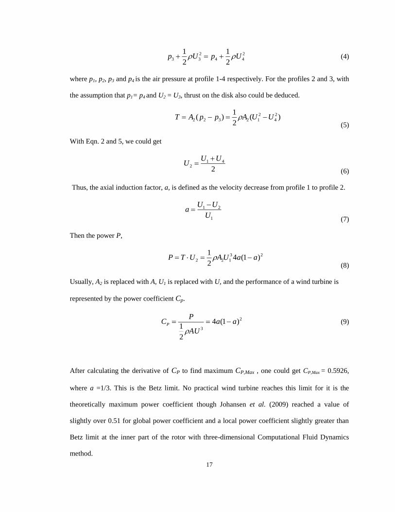
where p1, p2, p3 and p4 is the air pressure at profile 1-4 respectively. For the profiles 2 and 3, with
the assumption that p1= p4 and U2 = U3, thrust on the disk also could be deduced.
)(2
1)( 2
4
2
12322 UUAppAT (5)
With Eqn. 2 and 5, we could get
2
412
UUU
(6)
Thus, the axial induction factor, a, is defined as the velocity decrease from profile 1 to profile 2.
1
21
U
UUa
(7)
Then the power P,
23
122 )1(42
1aaUAUTP
(8)
Usually, A2 is replaced with A, U1 is replaced with U, and the performance of a wind turbine is
represented by the power coefficient Cp.
2
3
)1(4
2
1aa
AU
PCP
(9)
After calculating the derivative of CP to find maximum CP,Max , one could get CP,Max = 0.5926,
where a =1/3. This is the Betz limit. No practical wind turbine reaches this limit for it is the
theoretically maximum power coefficient though Johansen et al. (2009) reached a value of
slightly over 0.51 for global power coefficient and a local power coefficient slightly greater than
Betz limit at the inner part of the rotor with three-dimensional Computational Fluid Dynamics
method.

18
Using similar methods, the axial thrust T on the disk at position 2 could be deduced. The thrust
coefficient CT is defined to indicate the thrust, as shown in Eqns. 10 and 11.
22 )1(42
1aaAUT (10)
)1(4
2
1 3
aa
AU
TCT
(11)
3.1.2 Wake rotation
In 3.1.1, the wake rotation is not considered to influence the air flow. Actually, wake rotation
analysis is another method to calculate wind turbine power, and was developed initially by
Glauert in 1935. When an annular stream tube at the rotor plane (profiles 2 and 3) is taken out,
the thrust on an annular element is dT.
rdrrdAppdT 2)2
1()( 2
32 (12)
Where r is the radius of the blade, dr is the thickness, Ω is angular velocity of the wind turbine
rotor, and ω is the angular velocity of the wind. Similarly, a’ is defined as angular (or tangential)
induction factor, defined as:
2'
a (13)
Substituting Eqn. 13 into Eqn. 12, we get:
drraadT 32)'1('4 (14)
With the analysis in 3.1.1 axial momentum also could be defined as
rdraaUdT )1(42 (15)
With Eqns. 14 and 15, local speed ratio λr is defined as:
19
2
1
])'1('
)1([
aa
aa
U
rr
(16)
Then, tip speed ratio is,
U
R (17)
From the conversation of angular momentum, the torque on the annular element is dQ,
rrrdrUrrmddQ ))(2()( 2 (18)
When Eqns. 7 and 13 are substituted in Eqn. 18,
drrUaadQ 3' )1(4 (19)
3.2. Blade element theory
The BEM was also from blade element theory, and was developed with these assumptions: each
element is independent of the others, with no radial interaction, and almost constant axial flow
induction factor (Burton et al., 2001).
3.2.1 Airfoil
The airfoil is the most important and fundamental element in building a wind turbine blade.
Airfoil characteristics will determine the performance of the wind turbine, expressed in terms of
CT and CP. Lift coefficient and drag coefficient of airfoil are the central for designing a wind
turbine and the foremost parameters to be considered. These coefficients depend on Reynolds
number. In fluid dynamics, non-dimensional Reynolds number is defined as
UL
v
ULRe (20)
where is fluid viscosity, ρ is the fluid density, and v is the kinematic viscosity, U is the velocity
of fluid passing the airfoil surface, L is the length of the flow. L will be replaced by the chord
length c in terms of wind turbine blade.

20
Lift coefficient and drag coefficient could be measured in two-dimension or three-dimension. In
rotor design, two-dimensional coefficients are adopted widely. They are defined as followed.
lengthunitforceDynamic
lengthunitforceLift
cU
lLCl
/
/
2
1
/
2
(21)
lengthunitforceDynamic
lengthunitforceDrag
cU
lDCd
/
/
2
1
/
2
(22)
Where Cl is lift coefficient, Cd is drag coefficient, l is the airfoil span.
The lift coefficient and drag coefficient of an airfoil are a function of the angle of attack and
Reynolds number. Airfoil behaviour in the air flow is divided into three phases: the attached flow
phase, the high lift/stall development phase and the flat plate/fully stalled phase (Manwell et al.,
2002). In small wind turbine design, designers prefer high lift coefficient and relatively low drag
coefficient at low angle of attack, and try to operate with the airfoil in the attached flow phase if
possible, though some stall-regulated wind turbines operate in high lift/stall development phase.
3.2.2 Blade element analysis
As shown in Fig. 5, the following relationships among the parameters can be determined as below
(Manwell et al., 2002).
0,ppT (23)
p (24)
ra
a
ar
aU
)'1(
1
)'1(
)1(tan
(25)
21
])'1(
1[tan 1
ra
a
(26)
sin/)1( aUUrel (27)
cdrUCdF rellL
2
21 (28)
cdrUCdF reldD
2
21 (29)
sincos DLN dFdFdF (30)
cossin DLT dFdFdF (31)
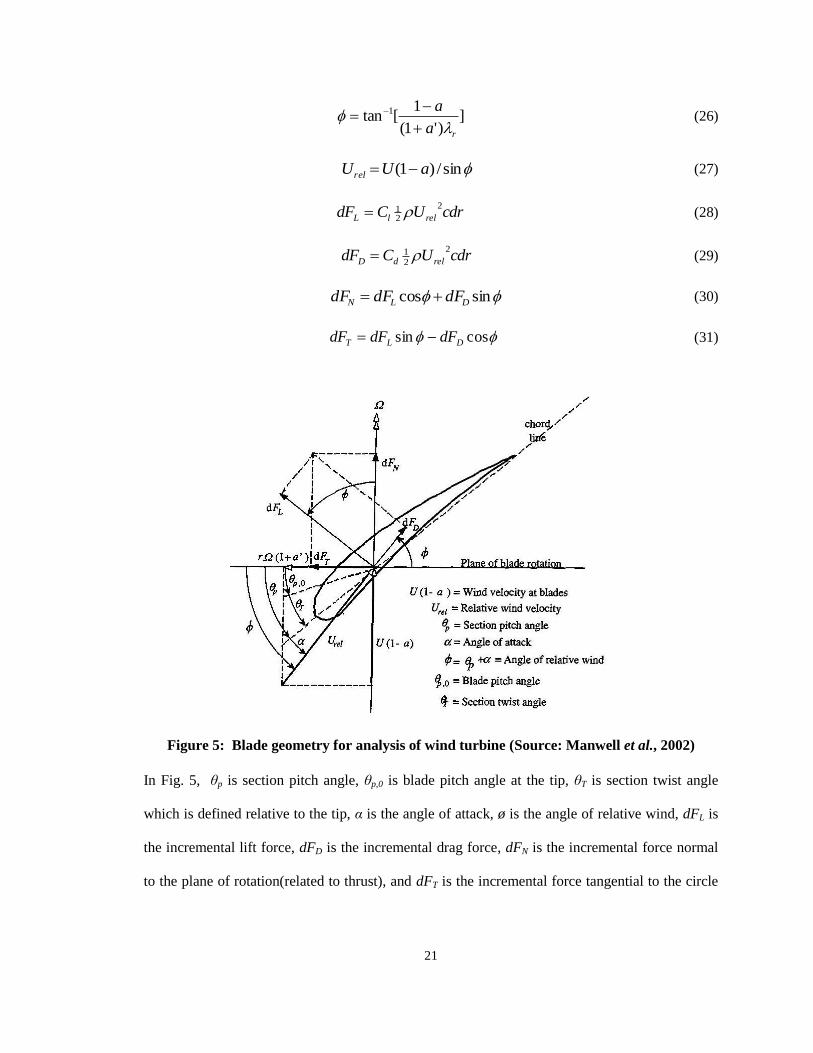
Figure 5: Blade geometry for analysis of wind turbine (Source: Manwell et al., 2002)
In Fig. 5, θp is section pitch angle, θp,0 is blade pitch angle at the tip, θT is section twist angle
which is defined relative to the tip, α is the angle of attack, ø is the angle of relative wind, dFL is
the incremental lift force, dFD is the incremental drag force, dFN is the incremental force normal
to the plane of rotation(related to thrust), and dFT is the incremental force tangential to the circle
22
swept by the rotor, which contributes to the useful torque, Urel is the relative wind velocity, U(1-
a) is wind velocity at blades.
If the rotor has B blades, the total normal force on the local radius r is,
rdrCaU
rdrCCaU
dF ndlN
2
22
2
22
sin
)1()sincos(
sin
)1(
(32)
The differential torque from the tangential force at local radius r, is
drrCaU
drrCCaU
dQ tdl
2
2
222
2
22
sin
)1()cossin(
sin
)1(
(33)
Generally normal load coefficient Cn and tangential load coefficient Ct are defined as (Hansen,
2008),
sincos dln CCC (34)
cossin dlt CCC (35)
And σ is the local solidity, defined by:
rBc 2/ (36)
Where, c is chord length of blade at radius r.
3.3. Blade element momentum theory
From Eqns. 15 and 32, dFN=dT and Eqns. 19 and 33, dQ=dQ, two equations can be obtained as
below (Hansen, 2008).
1sin4
1
1)sincos(
sin4
122
ndl CCC
a
(37)
1cossin4
1
1)cossin(
cossin4
1'
tdl CCC
a
(38)

23
In some cases to simplify the calculation, Cd could be negligible without affecting the calculation
of a and a’ (Manwell et al., 2002), then the above two equations become,
1cos
sin4
12
lC
a (39)
1cossin4
1'
lC
a
(40)
3.4. Loss factors
An actual wind turbine blade experiences three dimensional aerodynamic effects, especially near
the hub and tip. Loss factors can be included in the BEM, specifically tip and hub loss factor, to
account for these effects. Almost all the performance analysis of horizontal axis wind turbines
takes the tip loss factor into account because it tends to have a significant impact on results
(Manwell et al., 2002, Hansen, 2008, Lanzafame, 2009, and Martinez, 2005). The most popular
method was developed by Prandtl. With this method a correction factor for tip loss, Ftip could be
included into the previous equations (Dai et al., 2011).
]}sin)/(2
)/1({exp[cos
2 1
Rr
RrBFtip
(41)
Hub loss factor is more often neglected. Prandtl also developed an equation similar to tip loss
factor to calculate hub loss factor, Fhub (Dai et al., 2011).
]}sin2
)({exp[cos
2 1
r
RrBF hub
hub
(42)
The total loss factor is F,
tiphub FFF (43)
Then, Eqns. 37 and 38 could be written as
24
1sin4
12
nC
Fa
(44)
1cossin4
1'
tC
Fa
(45)
If Cd is very small and could be neglected, then Eqns. 44 and 45 become,
1cos
sin4
12
lC
Fa (46)
1cossin4
1'
lC
Fa
(47)
3.5. Turbulent wake state
In the stable operating condition, when the axial induction factor is smaller than a certain value,
Eqns. 44 and 46 work well. However, at turbulent wake states, these equations are not valid.
Glauert, Wilson and Buhl developed different empirical equations to calculate the axial induction
factor and thrust coefficient respectively (Hansen, 2008; Spera, 1994; Buhl, 2005). Shen et al.
(2005) also put forth another expression to correct the axial induction factor, but Clifton-Smith
(2009) questioned those equations highly in the viewpoint of aerodynamics. So the method of
Shen et al. is not included in this study.
3.5.1 Glauert method
Glauert developed an empirical equation (Manwell et al., 2002),
)889.0(6427.00203.0143.0)[/1( TCFa (48)

25
This equation is valid for a>0.4 or CT >0.96, where F is Prandtl’s loss factor. The local thrust
coefficient is defined as:
22 sin/)sincos()1( dlT CCaFCr
(49)
Eqns. 48 and 49 are used widely in the iterative application of BEM methods.
3.5.2 Wilson-Walker method
In 1994, Spera found an expression about thrust coefficient CT base on the axial induction factor a
(Hansen, 2008).
ccc
c
TaaFaaa
aaFaaC
))21((4
)1(4{
2 (50)
Where, ac is about 0.2 and F is the Prandtl’s loss factor.
If a> ac =0.2, then a should be calculated with below equation,
])1(4)2)21(()21(2[5.0 22 ccc KaaKaKa (51)
Where:
nC
FK
2sin4
The comparison of thrust coefficient CT from different expressions versus the axial induction
factor a is shown in Fig. 6 (Hansen, 2008).
3.5.3 Buhl method
In 2005, Buhl also developed a relationship for CT and a (Buhl, 2005).
2)49
50()
9
404(
9
8aFaFCT (52)
With Eqns. 49 and 52, axial induction factor a could be expressed as below (Dai et al., 2011).

26
)sin36sin509(2
sin48sin36sin186sin40sin3618222
43442222
FFC
FFCFFFCa
n
nn
(53)
These equations are valid when a>0.4. Buhl’s method was also recommended by Lanzafame and
Messina to eliminate the numerical instability that could occur when using Glauert method
(Lanzafame and Messina, 2007).
Figure 6: Different expressions for the thrust coefficient vs. the axial induction factor
(Source: Hansen, 2008)
3.5.4 The tangential induction factor
In the turbulent wake state, Eqns. 45 and 47 are still valid. Lanzafame and Messina (2007)
deduced another equation to calculate a’.
)1)1(4
1(2
1'
2 aaa
r (54)
Refan (2009) calculated a small wind turbine with optimized blade using this equation. However,
this equation is not as stable as Eqns. 45 and 47 because it includes a to calculate a’ within the
iteration process when simulating a blade like the Bergey XL 1.0.
27
3.6. Power coefficient
When a is determined, power coefficient Cp can be calculated by the equation
hr
l
drp d
C
CaaFC ]cot1)[1('
8 3
2
(55)
where λh is the local speed ratio at hub. Eqn. 55 can be modified into the following form to
simplify numerical solution.
]cot1)[1('8 3
1
l
dr
N
i
hp
C
CaaF
NR
RRC
(56)
where the blade is evenly divided into N sections of identical width, R is rotor radius, and Rh is
the radius of hub.
3.7. Simulation methods
The necessary equations for a BEM simulation have been discussed in the previous sections.
These equations can be used to predict the performance of a particular blade, and then determine
the wind power curve to judge the performance of the wind turbine design. The calculation
process follows the steps outlined immediately below. Because each blade element is assumed
independent from the others, the coefficients of each element are calculated separately. Finally
the global power coefficient is found by integrating results from the individual sections for the
specified tip speed ratio.
1) Initialize a and a’, typically set a=a’=0;
2) Calculate the flow angle ø with the Eqn. 26;
3) Calculate the angle of attack α using Eqn. 24;
4) Get Cl and Cd at α, if possible, Reynolds number should be considered.

28
5) Recalculate a and a’ with Eqns. 46 and 47 if neglecting drag coefficients, otherwise use
Eqns. 44 and 45. When Eqns. 44 and 46 are not valid, one of three methods for wake
state should be applied by choosing the relevant equations 48 ~ 54.
6) Repeat step 2~5 until changes in a and a’ are lower than the required tolerance.
7) Save the final a and a’ at each sections.
8) Calculate CP using Eqn. 56.
9) Using these methods, CP can be calculated across a range of tip speed ratios. Once these
calculations are completed, the curve CP ~ λ is easily plotted.
29
Chapter 4. Performance simulation of Bergey XL 1.0
4.1. Introduction
In the market of small wind turbines, Bergey XL 1.0 (sometimes “Bergey” in this thesis)
developed by Bergey Windpower Co., is the most popular: its blade structure is relatively simple
with constant chord and without twist (Bergey, 2011). However, the working situation is more
complex than optimized wind turbine blades for the angle of attack of the Bergey blade will vary
considerably spanwise whereas blades with optimized twist will not change as much as the
Bergey. Bergey XL 1.0 performance has been studied widely and it is often used as a reference in
comparisons with other wind turbines because it is mechanically and electrically straight forward
(Sharma and Madawala, 2007; Humiston and Visser, 2003; Nichita et al., 2006; Martinez et al.,
2006). In this study, modified Blade Element Momentum (BEM) methods was applied to
simulate the performance of the Bergey XL 1.0. Also the comparison among different
researchers’ analysis was performed.
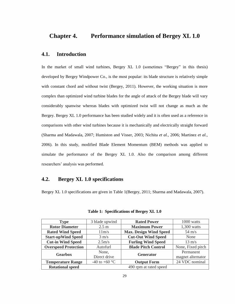
4.2. Bergey XL 1.0 specifications
Bergey XL 1.0 specifications are given in Table 1(Bergey, 2011; Sharma and Madawala, 2007).
Table 1: Specifications of Bergey XL 1.0
Type 3 blade upwind Rated Power 1000 watts
Rotor Diameter 2.5 m Maximum Power 1,300 watts
Rated Wind Speed 11m/s Max. Design Wind Speed 54 m/s
Start-upWind Speed 3 m/s Cut-Out Wind Speed None
Cut-in Wind Speed 2.5m/s Furling Wind Speed 13 m/s
Overspeed Protection Autofurl Blade Pitch Control None, Fixed pitch
Gearbox None,
Direct drive Generator
Permanent
magnet alternator
Temperature Range -40 to +60 °C Output Form 24 VDC nominal
Rotational speed 490 rpm at rated speed

30
4.3. Airfoil of Bergey XL 1.0
4.3.1 Geometry of Bergey airfoil
Bergey uses a patented airfoil SH3045; the theoretical geometry of the airfoil is not available. The
blade of a test Bergey was measured, interpolated when necessary as the leading and trailing
edges, and input into XFOIL software to predict lift and drag coefficients. The blade profile used
in this study is shown in Fig. 7. Seitzler and Kamisky (2008) also measured the airfoil to calculate
the performance using XFOIL. Martinez et al. (2006) measured the Bergey airfoil and made up
the trailing edge with airfoil NACA 7409.
Figure 7: Profile of Bergey XL 1.0
4.3.2 XFOIL
Lift coefficient and drag coefficients of an airfoil as a function of angle of attack are the most
important parameters characterizing an airfoil, because these parameters can determine the
power, the stall point, and the thrust. Ideally, researchers test the airfoil in a wind tunnel over a
range of Reynolds numbers and surface conditions to get data for accurate design and assessment.
The alternative method is to use one of several software applications that rely on potential flow

31
techniques or CFD to predict airfoil performance. XFOIL, a potential flow based solver available
free of charge, is perhaps the most popular software for this purpose (Drela, 2006).
XFOIL was written by Mark Drela with Fortran 77 in 1986 as an interactive program to design
and analyze subsonic airfoils. The main functions include (Drela, 2001):
Viscous (or inviscid) analysis of an existing airfoil.
Airfoil design and redesign by interactive specification of a surface speed distribution via
screen cursor or mouse.
Airfoil redesign by interactive specification of new geometric parameters - Blending of
airfoils.
Drag polar calculation with fixed or varying Re and/or Mach numbers.
Writing and reading of airfoil geometry and polar save files.
Plotting of geometry, pressure distributions, and polars.
At beginning, XFOIL could only run in UNIX operating system in workstation, now it works
well in Windows in common PC as long as the computer meets the minimum requirements for
this software.
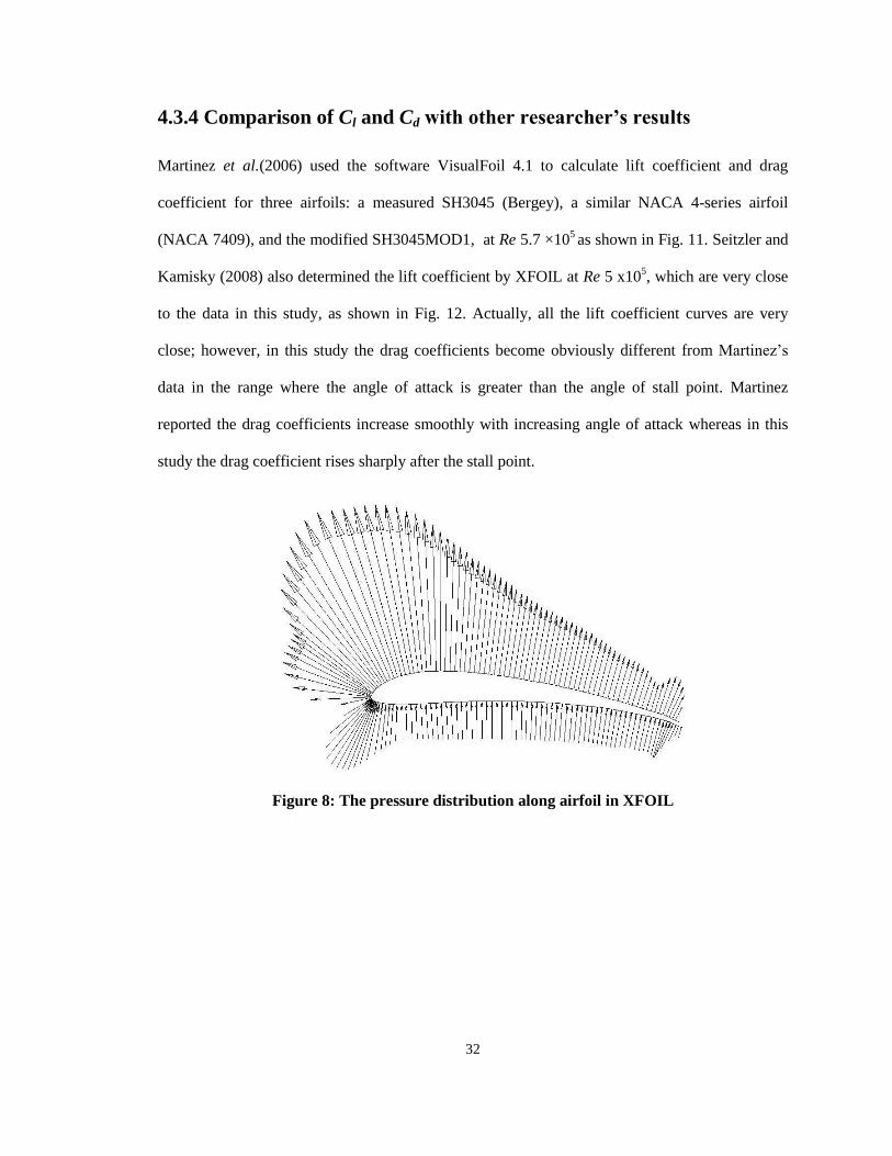
4.3.3 Cl and Cd of the Bergey airfoil
XFOIL can calculate the pressure along the airfoil surface and then integrate these values to get
Cl and Cd after basic airfoil data is defined clearly in the required format and Re number is
specified. Fig. 8 is one of the pressure distribution diagrams from an XFOIL calculation of Cl and
Cd for the Bergey airfoil. When Re ranges from 4×10⁵ to 6×10
5, the lift coefficient and drag
coefficient versus the angle of attack are shown in Figs. 9 and 10 respectively.
32
4.3.4 Comparison of Cl and Cd with other researcher’s results
Martinez et al.(2006) used the software VisualFoil 4.1 to calculate lift coefficient and drag
coefficient for three airfoils: a measured SH3045 (Bergey), a similar NACA 4-series airfoil
(NACA 7409), and the modified SH3045MOD1, at Re 5.7 ×10⁵ as shown in Fig. 11. Seitzler and
Kamisky (2008) also determined the lift coefficient by XFOIL at Re 5 x10⁵, which are very close
to the data in this study, as shown in Fig. 12. Actually, all the lift coefficient curves are very
close; however, in this study the drag coefficients become obviously different from Martinez’s
data in the range where the angle of attack is greater than the angle of stall point. Martinez
reported the drag coefficients increase smoothly with increasing angle of attack whereas in this
study the drag coefficient rises sharply after the stall point.
Figure 8: The pressure distribution along airfoil in XFOIL

33
Figure 9: Lift coefficient of Bergey airfoil
Figure 10: Drag coefficient of Bergey airfoil
Common sense suggests the data in this study is more reasonable because it is well known that
after the stall point both drag coefficient and lift coefficient change dramatically in opposite
directions (Burton et al., 2001; Hansen, 2008; Manwell et al., 2002). In addition, the angle of
attack at the stall point in Martinez’s figure is a little greater than that in this study. The difference
is believed to be partly due to the difference between the shapes of two airfoils near the trailing
edge.
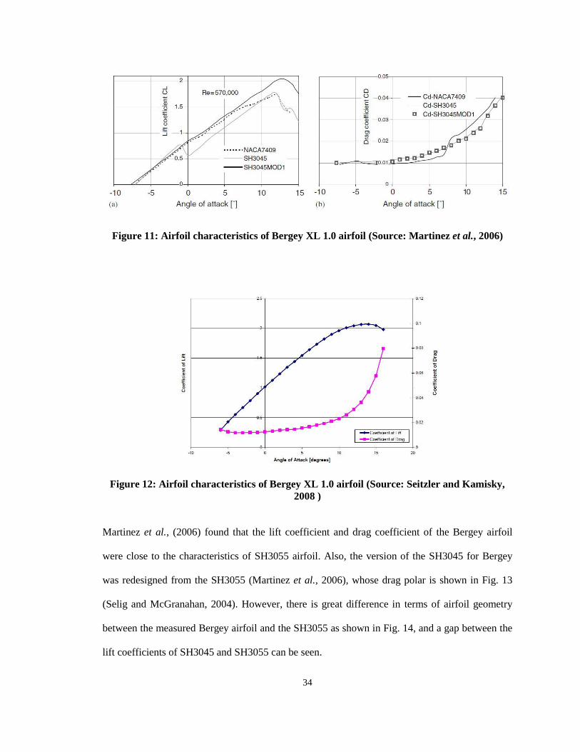
34
Figure 11: Airfoil characteristics of Bergey XL 1.0 airfoil (Source: Martinez et al., 2006)
Figure 12: Airfoil characteristics of Bergey XL 1.0 airfoil (Source: Seitzler and Kamisky,
2008 )
Martinez et al., (2006) found that the lift coefficient and drag coefficient of the Bergey airfoil
were close to the characteristics of SH3055 airfoil. Also, the version of the SH3045 for Bergey
was redesigned from the SH3055 (Martinez et al., 2006), whose drag polar is shown in Fig. 13
(Selig and McGranahan, 2004). However, there is great difference in terms of airfoil geometry
between the measured Bergey airfoil and the SH3055 as shown in Fig. 14, and a gap between the
lift coefficients of SH3045 and SH3055 can be seen.

35
Figure 13: Drag polar for airfoil SH3055 (Source: Selig and McGranahan, 2004)
Figure 14: Measured Bergey airfoil (‘x’ and solid line) and SH3055 airfoil (dashed blue line)
4.3.5 Lift and drag coefficient determination
Under normal operating conditions, local Reynolds numbers along the blade are typically within
the range of 1×10⁵ to 6×10
5. Over this range of Reynolds numbers, the lift and drag coefficients
vary little. Lift and drag coefficients at Reynolds number 5×10⁵ were used. This Reynolds
number is close to that used in Martinez’s analysis and the same as Seitzler and Kamisky’s.
XFOIL could calculate theoretically all lift coefficients and drag coefficients for angles of attack
from 0 to 360. However, after comparing the computational data with experimental data for
airfoil S809, it was found that the computational data before stall point, especially for small angle
of attack, was more reliable than those data over the stall point.

36
In order to simulate the performance of Bergey rotor, lift and drag coefficient at angles of attack
in the range from -5° to stall point (11.5°) can be fit to a mathematical function. Lanzafame and
Messina (2009) implemented a fifth-order logarithmic polynomial with the least square root
method to fit the experimental data. In this study, a spline function was implemented in Matlab to
produce continuous functions of the lift and drag coefficients versus angle of attack based on
tabular data, which is believed to be more accurate than the fitted equation since the possibility of
overfitting the data with too high order polynomial is avoided.
4.3.6 Lift and drag coefficients after stall
Accurately predicting blade performance requires prediction of airfoil lift and drag at angles of
attack above the stall point. One approach to this need is to use flat plate theory at angles of attack
greater than stall point (Wright and Wood, 2004). Assuming the airfoil behaves as a flat plate, the
lift and drag coefficients are easily calculated with the equations below, which are not Reynolds
number dependent.
cossin2lC (57)
2sin2dC (58)
The alternative method to calculate lift and drag coefficients after stall point is the Viterna
equations (Tangler and Kocurek, 2004; Martinez et al., 2004).
sin
cos2sin
2
21 AACl (59)
cossin 2
2
1 BBCd (60)
where:
α= αstall to 90° , for Bergey airfoil αstall=11.5°
)90(018.011.1max1
ARCB d
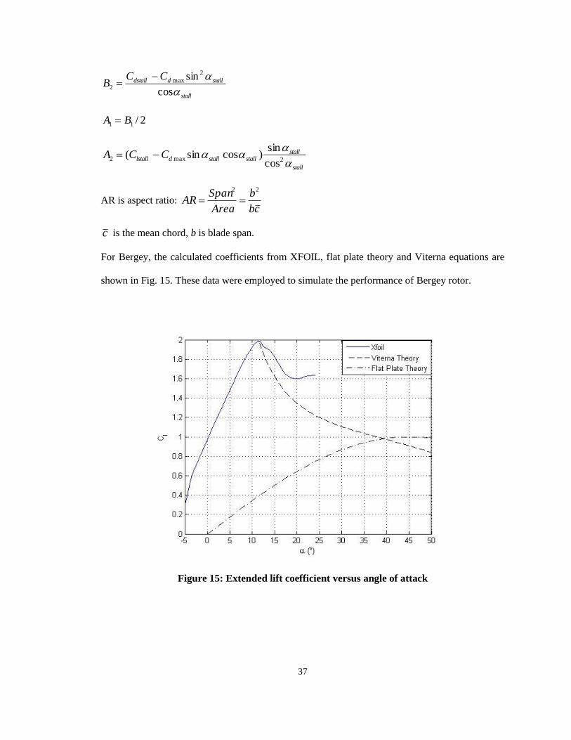
37
stall
stallddstall CCB
cos
sin 2
max2
2/11 BA
stall
stallstallstalldlstall CCA
2max2cos
sin)cossin(
AR is aspect ratio: cb
b
Area
SpanAR
22
c is the mean chord, b is blade span.
For Bergey, the calculated coefficients from XFOIL, flat plate theory and Viterna equations are
shown in Fig. 15. These data were employed to simulate the performance of Bergey rotor.
Figure 15: Extended lift coefficient versus angle of attack
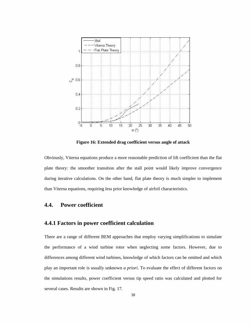
38
Figure 16: Extended drag coefficient versus angle of attack
Obviously, Viterna equations produce a more reasonable prediction of lift coefficient than the flat
plate theory: the smoother transition after the stall point would likely improve convergence
during iterative calculations. On the other hand, flat plate theory is much simpler to implement
than Viterna equations, requiring less prior knowledge of airfoil characteristics.
4.4. Power coefficient
4.4.1 Factors in power coefficient calculation
There are a range of different BEM approaches that employ varying simplifications to simulate
the performance of a wind turbine rotor when neglecting some factors. However, due to
differences among different wind turbines, knowledge of which factors can be omitted and which
play an important role is usually unknown a priori. To evaluate the effect of different factors on
the simulations results, power coefficient versus tip speed ratio was calculated and plotted for
several cases. Results are shown in Fig. 17.

39
Figure 17: Comparison of power coefficients with different factors included
The “Reference” curve was calculated including all loss factors (tip and hub loss), drag
coefficient, and Buhl’s method was used to simulate wake state. In addition, for lift coefficients
and drag coefficients at angles of attack greater than 20°, flat plat theory was employed for all
calculations. The “Cd =0” curve was similar, except drag coefficients were set to zero during the
iteration while the other factors in “Reference” are included. Curve “F=1” was calculated by
setting total loss factor F=1 while including the other factors. The remaining two cases set Ftip =1
and Fhub =1, which had the effect of assuming no tip or hub losses respectively in the calculations.
It is apparent in Fig. 17 that the tip loss factor has a noticeable influence on the predicted power
coefficients, whereas, the hub loss factor appears to have a negligible contribution. In addition,
assuming zero drag also has an impact on the predicted power coefficient, though it is not as
important as tip loss factor.

40
In a similar analysis, Clifton-Smith suggested that tip loss factor could be neglected because in
their study they observed that power coefficient were typically improved only 0.4% when
ignoring tip loss (Clifton-Smith, 2009). However, the calculations for this study differ, showing
an increase in the power coefficients of about 10% in the main working tip speed ratio range of 4
to 7. It is believed that this difference stems from the simple non-twisted structure of Bergey
blade, and its resulting large variation in operating conditions along the span, whereas Clifton-
Smith employed an equation from Burton et al. to calculate an aerodynamically optimized blade
geometry which would experience relatively consistent angle of attack at all points on the blade.
4.4.2 Flat plate theory and Viterna method
Since lift coefficient and drag coefficient are critical inputs for the performance calculation, it is
essential that these data accurately represent the airfoil and will be used even at high angles of
attack. Since no experimental data could be located for Bergey airfoil, power coefficients were
calculated with flat plate theory and Viterna method for angles of attack associated with post-stall
point. The calculated results are shown in Fig. 18.
Figure 18: Power coefficient versus tip speed ratio with two methods for post-stall point

41
In Fig. 18, all the previously discussed factors, including drag and loss, and wake factor from
Buhl method were taken into account for calculation. At tip speed ratios less than 9, the CP
predicted by Viterna method is greater than that of Flat plate theory; at tip speed ratios over 9,
both methods produce similar results. It is believed that the Viterna method gives the more
accurate results, based on analysis of lift and drag coefficients.
4.4.3 Wake factor
Glauert, Wilson-Walker, and Buhl methods are popular methods to account for the effect of the
rotor wake. Power coefficients using these three methods are compared in Fig. 19, where all
factors are considered and lift and drag coefficients of post-stall are from Viterna method.
Figure 19: Power coefficient calculation with different wake factors
In Fig. 19, the curves of Glauert and Wilson-Walker are smoother than that of Buhl, which
predicts a CP plateau between tip speed ratios λ of 5.2 and 6.2. Overall, Glauert method produces
higher values than the others. Wilson-Walker underpredicts relative to Buhl when λ is smaller
than 3.4, however, when λ is greater than 3.4, Wilson-Walker increases quickly and becomes

42
almost the same as Glauert in the λ range from 4.5 to 6. Since Buhl is the last developed method
and is based on all the previous research, Buhl was chosen as the reference for later calculations.
Based on previous analysis, when calculating power coefficient and/or power, all factors
including hub and tip loss, drag coefficients will be taken into account; Buhl method and Viterna
method will be employed to simulate wake effect and post-stall airfoil characteristics
respectively. These methods will be incorporated in the reference cases later in this study.
4.4.4 Comparison with others’ research
Seitzler and Kamisky (2008) simulated Bergey power curves using BEM method and WT_Perf
software respectively. Their results are plotted in Fig. 20 along with the results of this study,
which are denoted as “Reference”.
Figure 20: Comparison of power coefficients
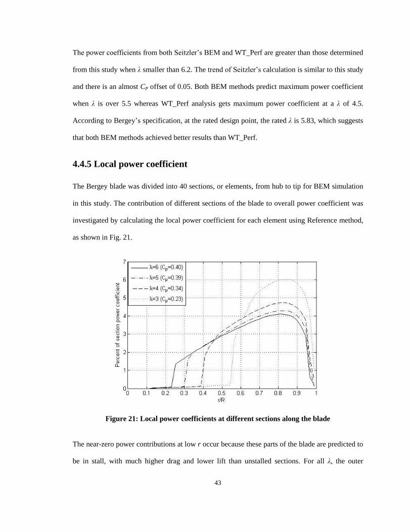
43
The power coefficients from both Seitzler’s BEM and WT_Perf are greater than those determined
from this study when λ smaller than 6.2. The trend of Seitzler’s calculation is similar to this study
and there is an almost CP offset of 0.05. Both BEM methods predict maximum power coefficient
when λ is over 5.5 whereas WT_Perf analysis gets maximum power coefficient at a λ of 4.5.
According to Bergey’s specification, at the rated design point, the rated λ is 5.83, which suggests
that both BEM methods achieved better results than WT_Perf.
4.4.5 Local power coefficient
The Bergey blade was divided into 40 sections, or elements, from hub to tip for BEM simulation
in this study. The contribution of different sections of the blade to overall power coefficient was
investigated by calculating the local power coefficient for each element using Reference method,
as shown in Fig. 21.
Figure 21: Local power coefficients at different sections along the blade
The near-zero power contributions at low r occur because these parts of the blade are predicted to
be in stall, with much higher drag and lower lift than unstalled sections. For all λ, the outer

44
sections of the blade have a greater contribution to the overall power. This is pronounced at the
lower λ. The start-up condition for this turbine occurs when the tip speed ratio is small (e.g. λ =
3). These results agree with Wright and Wood’s conclusion that most power producing torque
comes from the tip region (Wright and Wood, 2004).
4.5. Power simulation
Once the CP ~λ curve was calculated, the power production of the turbine at different wind speeds
with different tip speed ratio could be calculated easily. Additional assumptions had to be made
for this calculation. The maximum tip speed ratio was assumed to be 7 based on the experimental
data (discussed below). Atmospheric temperature was assumed to be 15°C, air density ρ = 1.225
kg/m3, and viscosity μ = 1.78×10
-5 kg/ms. Simulated rotor power at different rotor speeds was
calculated with these assumptions (Fig. 22).
Figure 22: Simulated rotor power at different rotor speeds

45
Martinez et al. (2006) calculated the curves for rotor power versus rotor speed shown in Fig. 23.
They tried using a constant Re and local variable Re, to calculate the power. At the same tip speed
ratio (e.g. same rotor speed and same wind speed), the powers predicted by Martinez et al. using
variable Re are similar or greater than the predicted power in this study, whereas Martinez et
al.’s predicted power using constant Re are greater than all data in this study. It was previously
noted that the airfoil characteristics change little over the Re range from 1×10⁵ to 6×10
5 within the
range of angle of attack from -5° to 10°, which is the major working region for the Bergey XL 1.0
airfoil. This suggests it is not necessary to use variable local Re in the BEM calculations for
Bergey if other factors are chosen correctly.
Figure 23: Simulated rotor power from Martinez et al. (Source: Martinez et al., 2006)
Nichita et al. (2006) also developed a simulation code and plotted the power vs. rotor speed
curves for Bergey as shown in Fig. 24. Based on their simulated data, they concluded that a blade
pitch angle of Bergey of 4° was needed for the rotor to produce the rated power at rated wind
speed. However, this result differs significantly from both this study and Martinez et al.’s results.

46
In this study, the constant pitch angle is set to 10° based on direct measurement of the Bergey
rotor and hub. This is the same angle used in Humiston and Visser’s research (Humiston and
Visser, 2003). Thus it is possible Nichita et al. found the wrong results with their simulation
methods, by simulating an incorrect condition. Consequently, their code is very questionable.
4.6. Field performance simulation
The simulations performed for this study were validated by comparison with field measurements
previously collected from an instrumented Bergey XL 1.0. Though performance analysis were
performed by other researchers (Martinez et al., 2006; Seitzler and Kamisky, 2008), they just
compared their simulated results with the published power curve by Bergey instead of comparing
that with the experimental data.
Figure 24: Simulated power of Bergey by Nichita et al. (Source: Nichita et al., 2006).
4.6.1 Efficiency of Bergey XL 1.0
The electrical efficiency of the Bergey turbine has to be characterized in order to be able to
extrapolate from rotor performance to predictions of overall turbine performance such as the
power curve. Sharma and Madawala (2007) computed that the efficiency of the Bergey generator

47
ranged from 0.63 to 0.50 at the rated design point and furling point respectively. Martinez et al.
(2006) analyzed Bergey XL 1.0 as a wind-electric battery charging system and measured the
curve of electrical efficiency versus the rotor speed as shown in Fig.25. Martinez’s experimental
data are chosen for use in this study because the data are directly measured, and Martinez
provided a detailed discussion of the process. Martinez’s data was used to produce the following
fitted equation.
6649.010635.110613.3 326
E (61)
Where, ηE is the efficiency of electrical system (also used as total system efficiency η), and Ω is
the rotor speed, in revolutions per minute.
Figure 25: Electrical system efficiency (Source: Martinez et al., 2006)
4.6.2 Test validation of simulation code
The performance data for a Bergey XL 1.0 installed in an open area near the University of Guelph
was collected for 4 months (Ziter, 2010) as part of a prior study. In the field test, wind speed,
rotor speed and electrical power output were recorded. It should be noted that the power output
by the turbine was dissipated by direct connection across a 2.01 resistor, rather than through a
maximum power point tracker, or the power centre supplied by Bergey with the XL 1.0 for

48
battery charging purposes. The test turbine was found to perform similar to other XL 1.0’s, except
for early onset of furling partially caused by an additional anemometer on top of the nacelle and a
solar panel on the turbine tail boom. Measured power output of this turbine is shown in Fig. 26.
For the simulation, wind speed and rotor speed data were binned from the original data and used
as input parameters to calculate the output power. The simulated results, the binned experimental
power and the manufacturer’s power curve from Bergey are shown in Fig.27.
The results showed that at wind speed less than 10 m/s, the computational data are very close to
manufacturer’s data. At wind speed greater than 10 m/s, all the simulated values are greater than
the rated values. However, the experimental data are different, which is to be expected because
the experimental data are based on a constant electrical load of 2.01 , rather than the optimum
loading that would be theoretically predicted, or supplied in practice by a maximum power point
tracker (Ziter, 2010). The simulation has assumed operation at the maximum power point after
the electrical efficiency is taken into account. There are also additional unavoidable sources of
error present in the field data, such as various turbulence levels, non-uniform inflow distributions,
wind shear and variable wind directions (Martinez et al., 2005), which partially account for the
scatter in Fig. 26. These effects impact the measurement and these influence cannot be entirely
eliminated even using binned, average data.
4.6.3 Local operating condition
Investigation of the field measurements found that a maximum λ of 6.57 occurred at a wind speed
of 8.24 m/s when the turbine was producing 424 W. The mean λ is 4.30. The binned λ versus
wind speed are plotted in Fig. 28. Also a three order curve was fitted using the least square just to
illustrate the trend.

49
With the experimental data, the real angle of attack at different wind speeds and the relevant tip
speed ratios were computed and plotted in the Fig. 29 with flat plate theory and in Fig. 30 with
Viterna method. Since the angle of attack should change smoothly along the span, Viterna
method is better than flat plate theory.
Figure 26: Original power data versus wind velocity
Figure 27: Power curves of simulation, manufacturer and binned experimental data

50
Figure 28: Tip speed ratio versus wind speed from the experimental data
Figure 29: Angle of attack along spanwise with flat plate theory

51
Figure 30: Angle of attack along spanwise with Viterna method
Access to measured turbine performance data also allows verification of the Reynolds number
assumptions made during the simulation process. The actual angles of attack at different wind
speeds, and the relevant tip speed ratios, were computed based on the measured data. This
information was used to verify the local Re spanwise along the blade, as shown in Fig. 31.
Though the Re for wind velocity of 5 m/s are lower than 1×10⁵ when r/R is smaller than 0.67, the
angle of attack exceeds the expected stall point of 11.5° when r/R is smaller than 0.48. It has
already been stated that when the angle of attack is high, the lift and drag coefficient are not
greatly dependent on Re. The Bergey XL 1.0 typically operates and produces power in wind
speed range from 5 m/s to 10 m/s. Within this speed range, the assumptions that Re is usually
between 1×10⁵ and 6×10
5 , and that a characteristic average Re for the blade would be
approximately Re = 5×10⁵ , appears to be reasonable.

52
Figure 31: Reynolds number along the blade at different wind speed and tip speed ratio
4.7. Discussion
The simulated power coefficient curve is not very smooth at some points, especially in the tip
speed ratio range of 5 to 6. This is because when the tip speed ratio increases, the local power
coefficient at the tip will decrease and local power coefficient close to the root increases. There
must be a trade off between these two opposing influences that results in an overall reasonable
power output. The method of calculating wake factor influences in the BEM simulation has a
noticeable impact on the results. Buhl method was found to be better than the Glauert and
Wilson-Walker methods for the case of the Bergey turbine.
The BEM process includes iterative solving of sets of equations. The numerical stability of the
iteration process depends on the properties of the lift and drag coefficient functions. For the
Bergey blade, angle of attack along the span varies significantly, and plays a very important role.
When local angle of attack is around stall point or becomes negative, getting the BEM code to

53
converge can become difficult. Sometimes the local power coefficient close to the tip becomes
negative. This is partially because Bergey is a non-twisted blade.
The power simulation is different from the measured field test data, primarily because of
differences in the electrical loading of the test turbine compared to a conventionally installed
turbine. This observation highlights the importance of detailed knowledge of the test turbine, and
attention to ensuring that the details of electrical loading and efficiency are accounted for correct
simulation. Simulation performance would also be improved by using experimental lift and drag
coefficient data including data under stalled conditions. However, in this study, XFOIL
simulations of Bergey XL 1.0 airfoil appear to have been adequate to get reasonably accurate
results, when used with a BEM simulation including loss factors and blade drag.
Compared with Clifton-Smith’s study, this study found that tip losses could not be ignored in the
analysis, and tip losses has a significant impact on performance, on the order of 10%. The results
presented here are consistent with Seitlzer and Kamisky, and Martinez et al., with difference
consistent with the use of different approaches to account for drag and tip losses. In addition,
Nichita’s arbitrary conclusion for Bergey XL 1.0 was questioned because it is not consistent with
the actual reported situation; consequently the calculations and method are doubted.
4.8. Summary of BEM method
The modified BEM method documented here was found to produce simulation results consistent
with the performance of the Bergey XL 1.0 as reported in the literature, given by the
manufacturer’s power curve, and observed from measurements of an instrumented Bergey XL
1.0.

54
Because the Bergey XL 1.0 blade has no twist, different parts of the blade can be operating at
widely ranging angles of attack, causing higher drag than would be experienced by a more
optimized rotor with twisted blades. For the Bergey XL 1.0 rotor, BEM analysis should not
exclude the tip loss, or make zero drag assumptions, as both of these factors have a significant
impact on predicted performance. The Buhl equation gave the best results among the three
methods investigated for evaluating the wake rotation.
It was observed that assuming a constant Reynolds number of 5×10⁵ for input lift and drag
coefficients gave similar results to the more data and computation intensive approach of using
local Reynolds number and Reynolds number dependent lift and drag coefficients. Both flat plate
theory and Viterna method worked well for calculating coefficients after the stall point: the
Viterna method gave somewhat better results, at the cost of additional complexity and the need
for more a priori knowledge of airfoil performance and blade structure.
Finally, the overall simulation results compared well to the actual performance of Bergey XL 1.0,
suggesting that XFOIL predictions of airfoil characteristics are sufficient as input for BEM
simulation of this turbine.

55
Chapter 5. New blade design
In this chapter, a new blade was designed for the Bergey XL 1.0 specifications, such as power,
diameter and tip speed ratio. In blade aerodynamic parameters determination, three methods were
considered and compared in structure and performance. After the design was completed, the
power performance was predicted for three different rotors, each using the new blade. The rotors
differed in the pitch angle at which the blades were mounted to the hub: for the three rotors, the
blades were joined to the hub at originally designed pitch angle (0°), and additional 5° and 9°
overall pitch angles.
5.1. Design specifications
The new blade design was designed to be retrofit to the Bergey XL1.0, so the design parameters
were chosen based on the specifications of this turbine. The Bergey XL 1.0 has a rated power of
1000 W at a wind speed of 11 m/s with a rotor diameter of 2.5 m. The new blade design was
planned for a length of 1.25 m from the center of rotation of the hub to the blade tip, to maintain a
2.5 m rotor diameter.
Most small wind turbines operate with a tip speed ratio λ between 4 and 10. At higher tip speed
ratios, the efficiency would be expected to increase, but this would be offset by higher noise
levels. The turbine generator is designed to produce power at particular tip speed ratios. Therefore
the new blade should be designed to operate at the similar tip speed ratios to the original Bergey
blades. The Bergey XL 1.0 with its original rotor operates at tip speed ratios between 4 and 7 at
wind speeds between 4 and 10 m/s (Ziter, 2010). Based on these values, the design tip speed ratio
was set to 5.85 when operating in an 11 m/s wind producing 1000 W.

56
Blade number will affect solidity of wind turbine and is related to balance of gyroscopic loads.
Two blades are cheaper to manufacture and easier to install than three blades installation;
however three blades can produce more power with smoother output (Maalawi and Badr, 2003).
Most horizontal axis wind turbines, including the Bergey XL 1.0, use three blades. The new rotor
was also designed to have 3 blades.
5.2. Airfoil selection
An appropriate airfoil section must be selected for the new blade design. Before beginning
detailed design of the new wind turbine blade, the configuration and airfoils used in existing
small wind turbines were reviewed. Table 2 summarizes the results of this review.
Table 2: Summary of small wind turbines in literature
Reference Airfoil Brief introduction Nation
Matsumiya et
al., 2010
SD 7037 1 kW rated power, 3.2 kW max. power. 1.8 m
diameter, 3 blades, carbon fibre composite.
Tested using vehicle.
Japan
Clifton-Smith,
2010
SG 6043 3 m diameter, 3 blades. Research for noise
reduction.
Australia
Kim et al.,
2010
Modified DU 91-
W2-250 & DU
93-W-210
6.4 m diameter, 10 kW rated power. Research
on noise reduction without power loss.
Theoretical analysis only.
Republic
of Korea
Refan, 2009 NACA6515(
root); GOE
228(middle); FX
63-137( tip)
2.2 m diameter, 3 blades, 1 kW rated power at
12.9 m/s. Multiple airfoil. Tested in wind
tunnel.
Canada
Lanzafame
and Messina,
2009
S 809 Two pitches (3° for tip section, 25° for root),
non-twisted blade, 5.03 m rotor radius. 10 kW
rated power.
Italy
Clifton-Smith
and Wood,
2007
SG 6043 3 m diameter, 3 blades, 2 kW rated power. Australia
Tangler and
Kocurek,
2004
S 809 5.03 m radius, 2 blades. Tested in wind tunnel,
Unsteady Aerodynamic Experiment (UAE)
project
U.S.
Wood, 2004 SD7062
3 m diameter, 2 kW rated power, 2 blades.
Designed for good starting performance and
power output. Used SG 6043 airfoil for initial
design.
Australia

57
Wright and
Wood, 2004
SD 7062 2 m diameter, 3 blades, 600W rated power at
10m/s. Research on starting and low wind
speed behavior.
Australia
Duquette and
Visser, 2003
SG 6043 2 m diameter, different numbers of blades
were applied to explore effects of solidity on
power coefficient.
U.S.
Oerlemans et
al., 2001
NACA 64418 4.5 m diameter, 2 blades. Research on noise
reduction
European
Project
DATA
Leftheriotis
and Carpenter,
1991
GOE 795 1.2 m diameter. NACA 4412, FX M2, GOE
795, E 193 and SOKOLOV airfoils were
investigated. GOE 795 was good for power
coefficient and high tip speed ratio (6.75)
U.K.
NB: In the table, some specifications are not complete because the authors did not list or not clear in
original paper.
Giguere and Selig (1998) specially designed four airfoils for small wind turbines: root airfoil SG
6040 and primary airfoil SG6041, SG6042 and SG6043 which had been applied by some
researchers in above table. Besides these airfoils, Selig and McGranahan (2004) tested six airfoils
used on small wind turbines, as shown in Table 3.
Table 3: Airfoil tested for small wind turbines (Source: Selig and McGranahan, 2004)
Airfoil Relevance/Usage
E387 Benchmark Eppler airfoil tested in NASA Langley LTPT
FX 63-137 Aeromag Lakota, Southwest Windpower H-40, H-80 and candidate for next
generation small wind turbine
S822 AOC/windlite, Havatex 2000 and candidate for next generation small wind
turbine, patented by DOE NREL
S834 New low-noise, low-Re airfoil and candidate for next generation small wind
turbine, patented by DOE NREL
SD 2030 Southwest Windpower Air 403 and Air X turbines
SH 3055 Bergey Windpower Excel turbine
Generally, thick airfoil sections do not have good performance at low Re, and airfoils of 20-25%
thickness should not be chosen (Wood, 2004). Thin airfoils with high camber would be expected
to produce more power with low thrust load (Maalawi and Badr, 2003).
58
Unfortunately, there was not a single consistent database or airfoil selection method in the
literature. To minimize risk and take maximum advantage of others’ experience, candidate
airfoils for the new blade design were evaluated on four points. Firstly, real wind turbine have
been produced and tested. Secondly, the size of wind turbine should be close to that of this study,
2.5 meter diameter or 1 kW rated power. Third, application of the airfoil would not infringe
patents or be expected to have to intellectual property issues. Finally, the airfoil should be thick
enough to provide a good reserve of strength in bending when operating, while still maintaining
good lift and drag characteristics.
With these points in mind, the range of candidate airfoils was minimized to SG 6043, SD 7062
and SD 7037. The SD 7037 has very high ratio of Cl/Cd at low Re number and excellent
aerodynamic performance for a small wind turbine. However, this is a very thin airfoil, which
would be expected to increase the difficulty of blade manufacture. Matsumiya et al. (2010)
produced their blades with carbon fibre composite because the thickness of this airfoil is 9.2%,
less than the 10.4% thickness of the original Bergey airfoil, which is also a very thin airfoil. The
SG 6043 as an excellent airfoil, has been used by U.S. and Australian researchers, and has high
Cl/Cd ratios at low Re over a broad range of angles of attack (Giguere and Selig, 1998). Wood
(2004) recommended that the SD 7062 airfoil would have good comprehensive performance: a
thickness of 14% provides more options for strengthening and manufacturing, and the airfoil has
good lift and drag characteristics at the Re typical for small wind turbines. Wood’s group changed
from SG 6043 to SD 7062 during their project (Wood, 2004). Balancing these factors, the SD
7062 airfoil was selected for the new blade design.
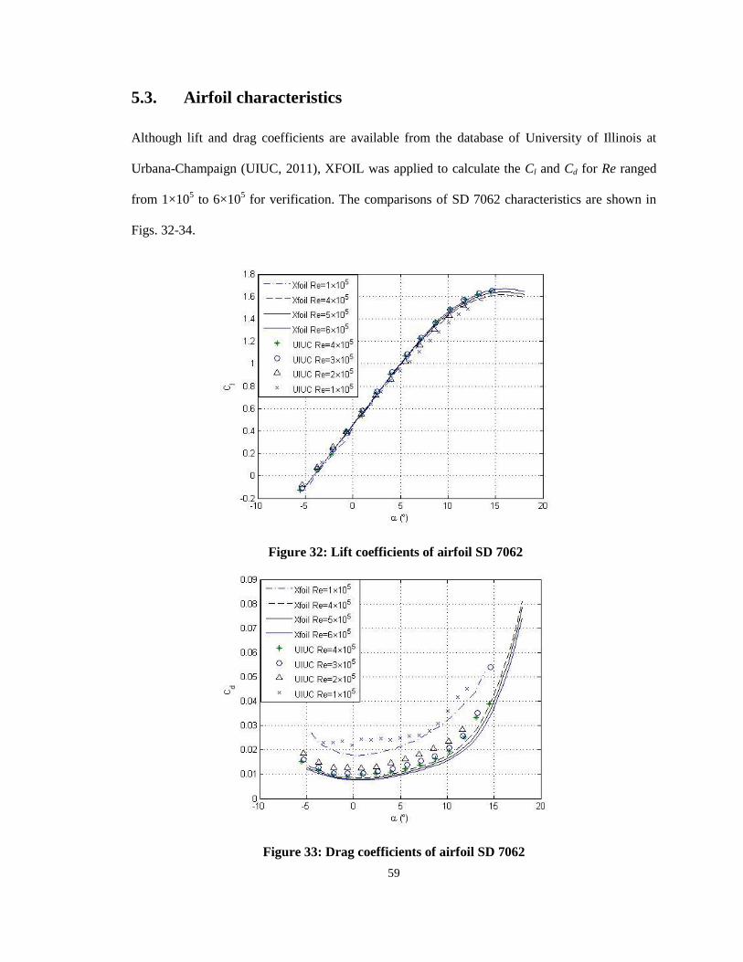
59
5.3. Airfoil characteristics
Although lift and drag coefficients are available from the database of University of Illinois at
Urbana-Champaign (UIUC, 2011), XFOIL was applied to calculate the Cl and Cd for Re ranged
from 1×10⁵ to 6×10
5 for verification. The comparisons of SD 7062 characteristics are shown in
Figs. 32-34.
Figure 32: Lift coefficients of airfoil SD 7062
Figure 33: Drag coefficients of airfoil SD 7062

60
Figure 34: Ratio of lift coefficient over drag coefficient for airfoil SD 7062
The lift coefficients predicted by XFOIL and those measured at UIUC are very close whereas
drag coefficients from XFOIL are generally lower than those measured by UIUC (2011). Since
the UIUC data is direct measurements of airfoil performance in a wind tunnel, rather than a
potential flow simulation, and is accepted by many researchers as reliable (Duquette and Visser,
2003; Clifton-Smith and Wood, 2007; UIUC, 2011), the UIUC data was applied in the design
calculations that followed.
5.4. Initial blade aerodynamic parameters
Once the input parameters for the BEM analysis have been determined, the BEM method can be
used to determine the blade shape, and then predict blade performance. For an airfoil, the ratio of
the lift and drag coefficients (Cl and Cd) is a function of angle of attack α (e.g. Fig. 34). For best
performance, the optimum angle of attack α occurs when Cl/Cd is maximum. When using BEM to

61
design a blade, selection of optimum α as a function of radial distance along the blade should
result in a blade that produces the maximum power CPmax (Manwell et al., 2010). The relevant lift
coefficient would be used in design as Cl,design .
The twist and chord distribution of a blade are determined with Eqns. 62-65 and 26.
14
31'
a
aa (62)
)14)(1('2
aaa r (63)
)1
'1
1(
r
ia
aarctg
(26)
rdesignl
ii
BC
rc
,3
sin8 (64)
Eqn. 64 can equivalently be written as,
designl
ii
BC
rc
,
)cos1(8 (64a)
- ii (65)
In above equations, subscript i denotes the parameters at section i. After inputting λr (the radius is
r) and Eqns. 62 and 63 are solved for a and a’ of the blade element at the radial position of r.
Then the angle of relative wind ø is calculated from Eqn. 26. Since lift coefficient Cl and angle of
attack α have been optimized and determined in advance, chord length ci and section pitch angle
θi can be determined by Eqns. 64 and 65.
In order to install and manufacture the blade easily, linear variation of chord and twist would be
better though this would slightly decrease power coefficient (Habali and Saleh, 2000). Manwell
et al. (2002) stated a method to get the linear relationships for taper and twist as below.
11 braci (66)
0,2 )( pi rRa (67)

62
where, θp,0 is the pitch angle at the blade tip, a1, b1 and a2 are linear coefficients from fitting all
chords and pitch angles calculated from equations 63-65 and 26 with least square regression
method.
Burton et al. (2001) provided a direct method to calculate the chord length c and pitch angle θ as
below.
BCR
c
l
r
2)2(
9
8
8.08.0
(68)
)1
3
21
3
11
(
2r
r
i arctg
(69)
Where λ0.8 is the local speed ratio at r=0.8R. For SD 7062 airfoil at Re= 4×10⁵ and α = 7.05, the
UIUC data gives a maximum Cl/Cd = 88.55 and Cl,design = 1.222. Then this point is set as design
point. In practice, the blade was divided into 20 elements and Matlab was employed to calculate
all the aerodynamic parameters.
Results of chords and pitch angles from three methods above are shown in Fig 35 and 36. Data
denoted as Optimal are calculated from Eqns. 62-65; data denoted with Fitted are from Eqns. 66
and 67 (a1 = -0.13, b1 = 0.20 and a2 =6.95); data denoted with Practical are from Eqns. 68 and 69.
It is evident that the Fitted method limits both chord and twist to linear variation whereas the
Practical approach keeps only the chord linear.
5.5. Initial performance prediction
To find the best structural parameters, the power performance expected for the three methods
(Optimal, Fitted and Practical) should be calculated and compared for decision making to get a
balance between efficiency and manufacturing complexity.

63
For the power performance predictions, the characteristics of the SD 7062 at Re = 4×10⁵ from the
UIUC data were used at angles of attack below the stall point at = 15.5°. Lift and drag
coefficients at angles of attack exceeding the stall point were calculated with the Viterna method.
The resulting lift and drag data are shown in Fig. 37.
For the three sets of aerodynamic parameters from the three methods, the CP ~ λ curves were
predicted when drag coefficients, wake factor of Buhl method were taken into account. The
resulting power curves, along with the power curve derived for the original Bergey XL 1.0 blades
(see Section 4.4), are plotted together for comparison in Fig. 38. Since the goal of this
comparison was to find the performance differences in the three types of blades, the same
constant Re= 4×10⁵ at all radial sections were applied to all blades.
Figure 35: Chord as a function of radius determined by the three methods

64
Figure 36: Twist as a function of radius calculated by the three methods
Figure 37: Extended airfoil characteristics of SD 7062

65
Figure 38: Power coefficient comparison for the new blade in 3 types of parameters and the
original Bergey blade
When tip speed ratio is less than 4.5, the original Bergey blade performs better than the new
blades, whereas at above 4.5, the new blades have higher power coefficient than the original
Bergey blades. Because the main range of for Bergey was from 4 to 7 according to the
measurements of Ziter (2010), the new blades would be expected to produce more power than the
original Bergey blades at high rotor speeds. Overall, the blades designed using the three methods
have very close power coefficients over the entire range of tip speed ratio.
5.6. Structural design of blade
5.6.1 Blade elements parameters
After comparing the performance (quantified as CP~) predicted for each of the three methods,
the blade design resulting from the Practical method was chosen because its structure would be
easier for building a blade. The overall depth and width of the Practical blade are smaller than the

66
Optimal blade, and the extreme surface angles are less (Figs. 35 and 36), meaning that a smaller,
simpler mould would be needed to build the Practical blade.
Design of the mould required determining the complete geometry of the blades. Knowing chord,
pitch angle and the airfoil section, the coordinates Xi and Yi of each profile could be reached by
substituting c of each element into the airfoil coordinates. The variable Xi is distance to the end
point on leading edge in the direction aligned with chord and axis Yi is the perpendicular to the
chord line. However, the twist angle of each element must be taken into account since usually the
three dimensional model is built at the same position as the blade is working. So the coordinates
of the airfoil profiles at each section have to be transformed to a consistent rotor-centered
coordinate system. In this rotating axis system, the X and Y coordinate directions are in the plane
of the airfoil section, and positive Z is the distance radially outward from the center of rotor
rotation. Eqns. 70-72 are used to translate the local airfoil coordinates to the rotor rotating axis
system with pitch angle θ for each element.
cYcXX ii ]sincos)25.0[( (70)
cYcXY ii ]cos)sin)(25.0[( (71)
rZ (72)
Applying these coordinate transformations to the Practical blade design results in the profiles
shown in Fig. 39.
5.6.2 Root design
The new blade was designed to be installed on the unmodified rotor hub of the Bergey XL 1.0.
The hub is a one piece casting with a curved surface designed to support the original Bergey
airfoil, which has a constant chord of 102 mm, at constant pitch angle of 10. For the new blade, a
smooth transition from the hub to the active part of the blade, easy installation and strength at the
blade root must be considered. A mixed airfoil was designed for the portion of the blade that
contacts the hub. The suction side of this airfoil is from the profile of the original Bergey airfoil,

67
while the pressure side uses the profile of the SD 7062 airfoil to allow smoother transition to the
working region of the blade. Three airfoils are shown in Fig. 40.
Figure 39: All profiles in rotor rotating coordinates system
Figure 40: Airfoils of new blade and Bergey
The mixed airfoil is also thicker than either the original Bergey airfoil or the SD 7062, which
allows for more material and greater strength than the original Bergey airfoil. To allow a smooth
transition from the mixed airfoil to the SD 7062 while still maintaining adequate strength, the

68
chord length was designed arbitrarily into a linear relationship with respect to blade radius (from
Rhub =130 to r = 200 mm). More information is reported in Appendix A.
5.6.3 New blade geometry
The transformed airfoil coordinate data for each section were input into Solidworks CAD
software, and used to generate a three dimensional solid model of the new blade design. The
result was the blade geometry which was fabricated, shown in Fig. 41.
Figure 41: 3D solid model of the new blade
5.7. Predicted performance of new blade
Having defined the detailed geometry of the new blade, the power curve of a rotor consisting of
three of the new blades was calculated by predicting rotor performance across a range of different
rotor speeds and different wind speeds. These predictions were completed assuming constant Re,
and also using local Re, which varied with wind speed, rotation speed and radial position along
the blades. However, the same results were reached with two methods to choose Re. In this
performance simulation, constant Re could be applied for this blade, in the same manner was

69
done in the simulation of the original Bergey blade (Chapter 4). The resulting power performance
is shown in Fig. 42.
Similar to the analysis of the original Bergey blade in Chapter 4, the local power coefficients at
different tip speed ratio were calculated spanwise for the new blade design in Fig. 43. At a tip
speed ratio of 3, local power coefficient generally increases continuously from root to tip (except
a short plateau) with maximum 11% at the tip whereas local power coefficients at higher tip
speed ratios increase steadily outward from the hub, but peak between r/R of 0.8 and 0.9, and
then decrease sharply in the region of the tip, indicating tip loss increase quickly at these sections.
Figure 42: Power simulation of the new blades

70
Figure 43: Local power coefficient comparison at different tip speed ratios
5.8. Performance comparisons at different pitch angle
Airfoil section, pitch angle and chord are the primary parameters of a wind turbine rotor (Wood,
2004). While details of the airfoil, chord and local pitch angle are fixed once the blade is
designed, in practice it is possible to change the overall pitch of the installed blades by changing
the inclination angle at which they are attached to the hub. In this way, the same blade can
provide a range of different performance characteristics. Practically, the new blade would be
installed on the Bergey turbine, but it was unknown whether the new blade matched well with the
alternator and the electrical load. Overall pitch angle of the blades is the only parameter that can
be adjusted in the test to account for these variables.
5.8.1 Power coefficient comparison
Performance of the new blade was predicted for assuming the blades were mounted to the hub at
the following pitch angles: 0° (as designed), 3°, 5°, 7°, 9°, and 11°. Fig. 44 shows the power

71
coefficient as a function of tip speed ratio for each of these pitch angles. The same curve
predicted for the original Bergey blade is also plotted in Fig. 44 for comparison. The
performance of the rotor with 3° additional pitch angle is very close to the original new blade (0°)
whereas the rotor with 5° additional pitch angle would produce a little higher power than Bergey
at tip speed ratios greater than 5. On the other hand, the rotors of 7°, 9°, and 11° additional pitch
angles produce less power than the original Bergey blade at all tip speed ratios.
Figure 44: Comparison of power coefficients
5.8.2 Performance comparison between new blades and Bergey
Based on Fig. 44, it was decided to test rotor with the original new blade (0° pitch angle), and
rotors with 5° and 9° additional pitch angles. The original Bergey rotor would also be tested for
comparison. Since the original Bergey blade was the reference, comparisons of performance
predictions at different rotor speeds and wind speeds were plotted in Figs. 45-47 respectively.
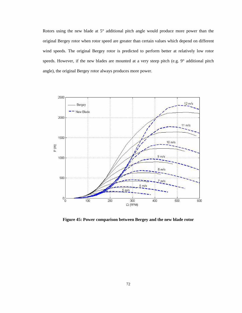
72
Rotors using the new blade at 5° additional pitch angle would produce more power than the
original Bergey rotor when rotor speed are greater than certain values which depend on different
wind speeds. The original Bergey rotor is predicted to perform better at relatively low rotor
speeds. However, if the new blades are mounted at a very steep pitch (e.g. 9° additional pitch
angle), the original Bergey rotor always produces more power.
Figure 45: Power comparison between Bergey and the new blade rotor

73
Figure 46: Power comparison between Bergey and the new rotor at +5° pitch angle
Figure 47: Power comparison between Bergey and the new rotor at + 9° pitch angle

74
Chapter 6. Blade fabrication and RTM system
Since the study documented in this thesis was part of project on Hierarchical Green Nano-
Biocomposites for Light Weight and Efficient Wind Turbines Blades, the manufacturing methods
used in this study should be applicable to a range of both conventional and biomaterials. Resin
transfer moulding (RTM) was utilized for blade production in this study in order to meet these
requirements. Information about the new blade design was detailed in Chapter 5. The mould
design was produced using Solidworks, and the stress and displacement of the mould in operation
was simulated by finite element method (FEM). Utilizing the mould with RTM, blades were
produced in fibreglass and epoxy composite.
6.1. RTM system design
6.1.1 Requirements of RTM system
Resin transfer moulding (RTM), also called resin injection molding (RIM), is a closed mould
process in which prepared reinforced material (cloth or fibres) is sealed in the mould, and then
resin is injected into the mould at low pressure (Rosato and Rosato, 2004). The pressure for resin
injection is about 0.69 to 1.38 MPa, and sometimes as low as 0.3 MPa. Pressure pushes the resin
through the reinforced material and fills the mould cavity with resin; an outlet in the mould
allows air in the mould to exit during filling. This process often is assisted with vacuum: in this
case the process is called (VARTM), and the vacuum helps to remove the entrapped air in the
mould and accelerate the resin flow (Strong, 1989). From the literature, RTM was not widely
applied in commercial small wind turbine blade production, however, this method has been
adopted in the past 20 years (Tangler, 2000). The related process of vacuum bagging has been
successfully and regularly used in the large wind turbine blade manufacturing (Brøndsted et al.,
2005).

75
All kinds of reinforcing fibres can be utilized in RTM, however fibreglass, carbon fibre and
aramid fibre are predominant; there are lots of resins available for use in RTM, the chief
requirements are that resin viscosities are generally lower than 1000 mPa·s and pot life is at least
two hours to avoid resin gel before the mould is adequately filled (Strong, 1989). The reinforcing
material can be stitched together to minimize movement and maintain shape when resins are
injected into the mould.
Compared to other methods for forming reinforced plastics, RTM has some advantages: it is good
for complex shapes, can have a short production time and achieve excellent surface definition,
and the mould can be produced from a variety of materials (Strong, 1989). On the hand, the
design of RTM moulds requires more skill compared to other types of moulds, and it is difficult
to control resin uniformity within the mould. Also, there are many variables in the process of
resin mixing and curing that can make RTM aging a little different each time (Rosato and Rosato,
2004).
Commercially, RTM has been developed into a complex system with process control, feeding and
cleaning, and additional support systems (Rosato and Rosato, 2004). However, simpler low
volume RTM systems equipped only with a ram or an airline can be also efficient and effective
(Strong, 1989).
6.1.2 RTM system utilized at University of Guelph
Fig. 48 shows a manually operated RTM (VARTM) system designed and used to make the
composite blades with commercial fibreglass and epoxy that were used in this study. The physical
system is shown in Fig. 49. The components in Fig. 48 are (1) compressed air supply, (2) air

76
filter, (3) pressure reducing valve, and (4) pressure meter. Throttle valves to control flow are
located at (5) and (11), and shut-off valves are located at (6) and (7). Item (8) is an air filter with a
liquid trap, (9) is a vacuum pump, (10) is the resin supply container and (12) is the actual RTM
mould assembly. In the future, bio-fibres and/or bio-resins can be utilized within the same system
with minimal modification.
Figure 48: RTM system
The general working procedure is described as below:
Before working on this system, shut off all valves.
Tailor fibreglass cloth and strand with respect to blade dimension, and place these
fibreglasses in the sequence to construct the shape of blade.
Stitch the fibreglass together to hold correct shape.
Put the stitched fibreglass assembly into the mould and close the mould assembly with
fasteners at the rated torque.

77
Check air leakage using compressed air and soap water to make sure mould sealed well.
Prepare resin following the required instruction and put it in Container 10.
Connect the RTM-VARTM system following Fig. 48.
Open Valve 6, vacuum resin Container 10 for 10 minutes, close Valve 6.
Open Valve 7, vacuum mould cavity for 10 minutes.
Open Valve 11, resin would flow into the mould.
Open Valve 5, and adjust Valve 3 to over 55 psi.
Close Valve 7 as soon as the resin comes out from mould over 10 centimetres in the tube.
After 10 minutes, or the resin does not flow in the tube, close Valve 11.
Close Valve 5.
Open mould and eject out the blade.
Figure 49: The physical RTM system at the University of Guelph

78
6.2. RTM mould design and production
The mould is the most important part of an RTM system: the mould structure will determine the
flow through reinforcement materials and the curing time of the resin (Strong, 1989). It is evident
that the shape of the mould is solely responsible for the geometry, tolerance and surface finish of
the parts made in the mould. Furthermore, the mould must withstand all loads from the resin
pressure, mould closure and stresses from chemical reaction of resin (Potter, 1997). For wind
turbine blades, the mould must be accurately made to ensure the correct blade shape and high
surface definition, on which the performance of a blade will depend directly.
6.2.1 Blade mould design
In this study, a multi-purpose mould was required that could be used for both hand lay-up and
RTM, and possibly could be utilized in a trial step for vacuum bagging in the future. Engineering
design of the mould requires carefully considering a range of factors, such as loads on mould
surface, heating methods for resin curing, mould cavity geometry, the sealing method between
mould halves, mould closure and clamping, ejection of mould and ejection of the worked part
(Potter, 1997).
The material for building the mould must be determined. Various materials have been used for
building moulds for RTM, including composites such as GRP and CFRP, and metals including
aluminum, steel and cast iron. Metals are the most popular (Potter, 1997). Three manufacturing
methods are possible depending on different requirements and cost-effective: direct machining
method using CAD/CAM, casting the mould from a master model, and hybrids of the previous
two methods (Potter, 1997).

79
The blade length in this study was 1.25 m and high geometric tolerances were required. A long
mould lifetime and low cost were also considered desirable. Aluminum 6061-T6 was chosen for
the material, because it is readily available and easy to work, with lower costs for CNC
manufacturing than steel.
A principle for mould design is to minimize the number of mould parts. For a two-part mould, the
separating profile should follow the largest extent of the part and allow easy splitting of the
mould. For this wind turbine blade, the mould was designed to split along extended profiles from
the trailing edge and the leading edge. This was chosen as a compromise, as this method is not the
best strictly for RTM because this structure makes it easy to accidentally pinch the reinforcement
material (Potter, 1997). However, this approach would work well for hand lay-up.
Considerations must be made for aligning and joining the two halves of the mould, and filling
resin and venting air during mould use. In the detailed design, two diagonal guide dowels were
included for aligning the two halves of the mould; extra processing holes were designed for
mould clamping and ejection; twenty four regularly spaced holes for bolt fixtures were positioned
around the edges of the mould. The flow route of resin was designed to be from blade root to tip,
and inlet and outlet ports were included to support these operations. The final 3-D drawing is
shown in Fig. 50.
6.2.2 Stress and displacement simulation of mould
Solidworks was used to simulate the stress and displacement of the mould assembly when in use.
The geometry of the mould was represented by a mesh containing 185,849 nodes, 122,077
elements, and 551,928 DOFs (model degrees of freedom). During RTM, the maximum inside
pressure from the compressed air would be less than 4 bar. The external load was set 60 psi and
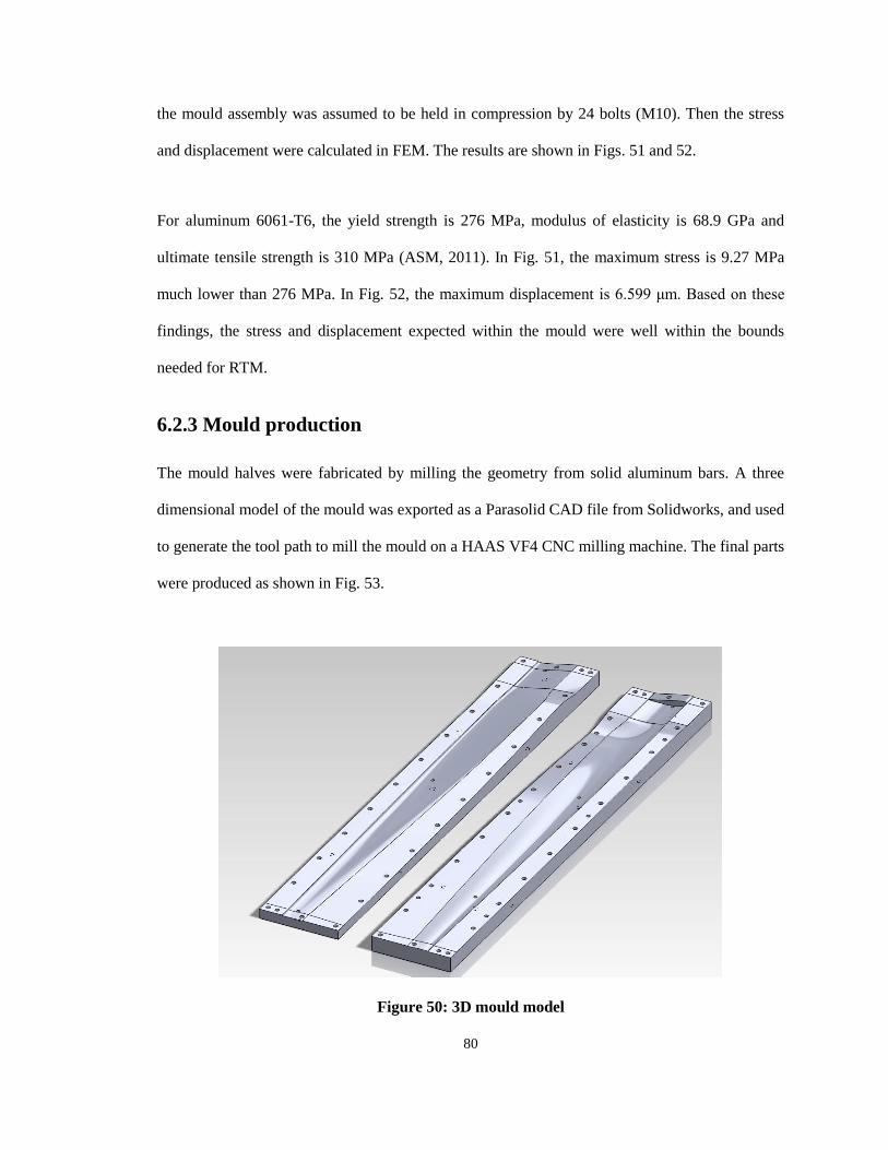
80
the mould assembly was assumed to be held in compression by 24 bolts (M10). Then the stress
and displacement were calculated in FEM. The results are shown in Figs. 51 and 52.
For aluminum 6061-T6, the yield strength is 276 MPa, modulus of elasticity is 68.9 GPa and
ultimate tensile strength is 310 MPa (ASM, 2011). In Fig. 51, the maximum stress is 9.27 MPa
much lower than 276 MPa. In Fig. 52, the maximum displacement is 6.599 μm. Based on these
findings, the stress and displacement expected within the mould were well within the bounds
needed for RTM.
6.2.3 Mould production
The mould halves were fabricated by milling the geometry from solid aluminum bars. A three
dimensional model of the mould was exported as a Parasolid CAD file from Solidworks, and used
to generate the tool path to mill the mould on a HAAS VF4 CNC milling machine. The final parts
were produced as shown in Fig. 53.
Figure 50: 3D mould model
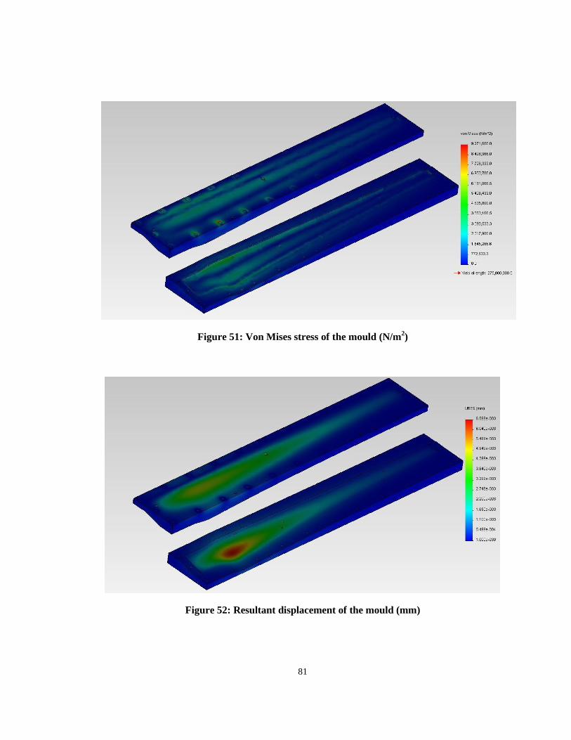
81
Figure 51: Von Mises stress of the mould (N/m2)
Figure 52: Resultant displacement of the mould (mm)

82
Figure 53: Aluminum mould made from CNC
6.3. Blade fabrication
After several trial mouldings, three blades for test purposes were fabricated using RTM methods.
Commercial fibreglass and epoxy resin (West System 105 Resin and 206 Slow Hardener) were
utilized following the procedure in section 6.1.2. To simplify the procedure, the blades were made
in solid profile, with fibreglass cloth reinforcing cut and fit in the mould prior to RTM. The
resulting blades are shown in Fig. 54.
6.4. Discussion
Pot life of the resin was an important consideration using the RTM approach. During the first trial
fabrication, Bondo resin (3M Company) was utilized, which has a pot life around 20 minutes. The
trial failed due to incomplete filling and variable quality in the resulting blade. The West System
epoxy, which has a much longer pot life, three blades were made well. However, bubbles were
found to occur on the blade surfaces and small pores were noted inside the blades. These defects
occurred because the vacuum pump could not evacuate all air that was mixed in the resin when

83
the resin was poured into the feed container prior to filling the mould. The best solution would be
to use a commercial RTM system in which the feed process is designed to avoid this occurrence;
the alternative is to enlarge the container and to install a blender in it to aid vacuum pump at
removing small air pockets.
Figure 54: Three blades made from RTM system at the University of Guelph
The curing time of epoxy resin depends on lots of variables, such as temperature, ratio of epoxy
to hardener and surrounding environment. When room temperature was a little lower than 15°C,
the resin took over one week to cure completely. Also it is not known how much the curing time
would affect the strength. In addition, it was noted that the solidification process was sensitive to
the mixing and concentration of the hardener. The epoxy would solidify sooner with just a little
more hardener, and vice versa.

84
After removal from the mould, final hand finishing of the blade surfaces, and drilling of three
mounting holes, the weights of three blades were 1504 g, 1486 g and 1501 g respectively. The
three original Bergey blades were 1480 g, 1470 g and 1478 g respectively. It is evident that the
solid blade would be heavier than one with a hollow or low density core; it is recommended that
the processing should be improved to produce lighter blades with a hollow profile later.

85
Chapter 7. Vehicle-based test
7.1. Introduction
Although the performance of a wind turbine could be simulated by BEM and CFD, the actual
measured performance is needed to validate and confirm the simulation results. For small wind
turbines, three test methods were found in the literature. One is wind tunnel testing, which has the
advantages of being able to precisely control wind velocities and measure wind turbine power
output with a minimum of confounding variables (Refan, 2009). However, to test a small wind
turbine requires very large wind tunnels, which are expensive to operate.
The most common approach to determine the performance of a small wind turbine is field testing,
which involves installing the wind turbine on a tower and measuring the actual results in natural
conditions. The performance will depend greatly on the installation site, and it can take many
months to collect enough data at all wind speeds to evaluate the performance of the wind turbine
(Ziter, 2010), but if there is sufficient time this is considered the best method to evaluate the
performance of the wind turbine.
A third method that can be used for small wind turbines is vehicle-based testing (Matsumiy et al.,
2010). In these tests, the wind turbine is installed on a tower that is fixed to a truck or trailer. The
performance of the turbine can be measured across a full range of wind speeds by driving the
vehicle at different speeds on a controlled course. This method is a rapid testing approach that can
be used to rapidly evaluate performance with relatively low costs.
Vehicle based testing was chosen to validate the new blade design. The developed testing
protocol required testing four different rotors, with two different types of blades (the original

86
Bergey blades, and the new blade design mounted to the hub at three different pitch angles).
Wind tunnel testing was not possible within the time and budget constraints of the project, and a
conventional field test would have required approximately two years of data collection, so
vehicle-based testing was selected as the most practical method for this study.
Only blades and pitch angles were changed between the four rotor configurations in this test: the
generator assembly of the Bergey XL 1.0 was not modified, and all tests were conducted on the
same day, on the same course, using the same sensors and measurement methods. Keeping non-
rotor variables constant allows direct performance comparisons among the different rotors, and
validation of the modified BEM simulation process.
7.2. Vehicle-based test system
7.2.1 Test road and weather
The vehicle-based test was conducted on February 2, 2012 at the south end of Southgate Drive, a
300-m straight paved road in Guelph, Ontario (Fig.55). With the exception of one set of power
line poles, there were no big trees, buildings or obstructions on either side of the road, and the
surroundings consisted of flat open fields. On the test day, average wind speed was observed to
be approximately 2 to 3 m/s from the north, temperature throughout the day was constant around
0°C. Relative humidity was between 72% and 78%, and it was mainly cloudy all day without rain
or snow (Environment Canada, 2012).
7.2.2 Test equipment and sensors
The vehicle-based testing platform consisted of a small car (2001 Ford Focus) towing a modified
two-axle draw bar equipped trailer on which a tilt up tower supporting the wind turbine was
placed. The test equipment and installation are shown in Fig 56. The hub height of the turbine

87
was 5.25 m above ground when the tower was upright for testing. A cup anemometer (NRG 40C
3-cup anemometer; S/N: 179500110821) served as the primary anemometer to monitor the wind
velocity. It was installed on a boom that located it 1.5 meters in front of the tower, 2.2 meters
behind the car and 2.32 meters above the car roof to minimize the effect of wake of car. The cup
anemometer was calibrated by the manufacturer (transfer function slope 0.756 m/s per Hz and
offset 0.34m/s).
Figure 55: Satellite view of surroundings at Southgate road test location in Guelph
An RM Young Model 81000 ultrasonic anemometer was also located on the car roof (Fig. 56) as
a secondary anemometer to measure three dimensional wind velocity and real-time temperature.
Before installing the anemometers, initial checkouts were conducted to confirm both
anemometers were correctly integrated with the data collection system. After testing, the
calibration of both anemometers was verified in the University of Guelph wind tunnel. Details on
calibration verification are reported in Appendix B.
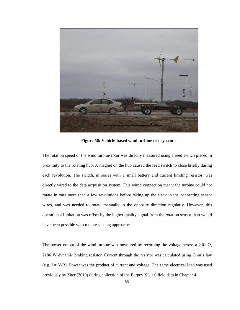
88
Figure 56: Vehicle-based wind turbine test system
The rotation speed of the wind turbine rotor was directly measured using a reed switch placed in
proximity to the rotating hub. A magnet on the hub caused the reed switch to close briefly during
each revolution. The switch, in series with a small battery and current limiting resistor, was
directly wired to the data acquisition system. This wired connection meant the turbine could not
rotate in yaw more than a few revolutions before taking up the slack in the connecting sensor
wires, and was needed to rotate manually in the opposite direction regularly. However, this
operational limitation was offset by the higher quality signal from the rotation sensor than would
have been possible with remote sensing approaches.
The power output of the wind turbine was measured by recording the voltage across a 2.01 ,
2186 W dynamic braking resistor. Current through the resistor was calculated using Ohm’s law
(e.g. I = V/R). Power was the product of current and voltage. The same electrical load was used
previously by Ziter (2010) during collection of the Bergey XL 1.0 field data in Chapter 4.

89
7.2.3 Data acquisition system
A National Instruments USB-6210 data acquisition system (DAQ) connected to a laptop
computer (Dell Latitude E5400; powered by a deep cycle battery and inverter) was used to record
analog signals from both anemometers, the wind turbine rotation speed sensor and the power
signal (voltage).
Since the wind turbine could produce transient voltages on the order of 40 V, the voltage across
the load resistor was determined using a voltage dividing circuit to ensure that the voltage input to
the DAQ would not exceed its 10 V sensing range. Wiring of this circuit is shown in Fig. 57.
The NRG anemometer outputs a variable voltage sinusoidal pulse with frequency proportional to
the wind speed. The ultrasonic anemometer and rotor speed sensor output voltage signal and
pulse signal respectively.
In this test, all measurement channels were sampled at a rate of 10,000 Hz for 3 second period for
the duration of each test run (30 seconds to one minute). A custom written Labview 8.6 program
stored all raw data, and summary data for each 3 second sampling period. The Labview program
used a Fast Fourier Transform to isolate the dominant pulse frequency of the NRG anemometer
and the wind turbine speed rotation sensor measurements in each 3 second sample and displayed
the real-time value on monitor. The raw data stored at 10,000 Hz was used to verify frequency
calculations.
7.2.4 Test methods and influential factors
During testing, the car was accelerated to reach the required wind velocity with respect to the
real-time wind velocity displayed on the computer monitor. Because the test route was only 300
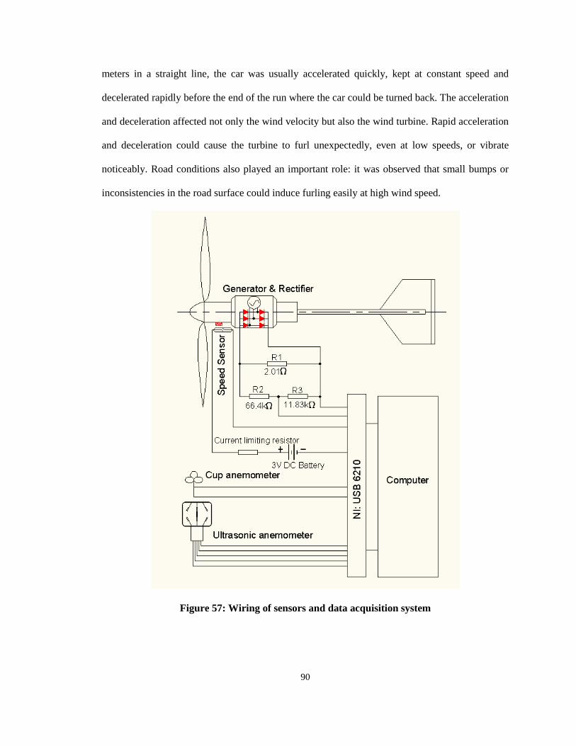
90
meters in a straight line, the car was usually accelerated quickly, kept at constant speed and
decelerated rapidly before the end of the run where the car could be turned back. The acceleration
and deceleration affected not only the wind velocity but also the wind turbine. Rapid acceleration
and deceleration could cause the turbine to furl unexpectedly, even at low speeds, or vibrate
noticeably. Road conditions also played an important role: it was observed that small bumps or
inconsistencies in the road surface could induce furling easily at high wind speed.
Figure 57: Wiring of sensors and data acquisition system

91
7.3. Measurement and uncertainty
7.3.1 NI USB 6210
In measurement, when assuming symmetric error, the true value of a variable x usually can be
expressed as:
xxx m (73)
Where xm is the measured value, x is the confidence interval of xm (uncertainty).
There are two sources of measurement uncertainty for a sensor. One source is the instrument
itself; the other is from the conversion of sensor signals from analog to digital. These two
uncertainties are assumed to be independent, and total uncertainty for a single measurement can
be calculated by Eqn.74 (Lira, 2002).
2
/
2
DAinstru xxx (74)
Where, x inst is uncertainty from instrument itself and xA/D is uncertainty from A/D conversion.
NI USB 6210 has 4 nominal analog sensing ranges. For this study, the range from -10V to +10 V
was selected. The equation for absolute uncertainty VDAQ (only related to measured voltage
values) due to analog to digital conversion in USB 6210 is (NI, 2009):
noiseoffsetrangegainreadingDAQ VVV (75)
where gain is gain error, offset is offset error and noise is noise uncertainty, unit V ; Vreading is
reading voltage and Vrange is the range of voltage (maximum positive value l0). Gain error, offset
error and noise uncertainty at maximum 10 V were taken as constants to calculate the absolute
uncertainty, meaning overestimation of errors would be expected. Substituting the assumed
values gives:
5.881303.132 rangereadingDAQ VVV (76)

92
At a full scale reading of 10 V, the absolute uncertainty would be 2711 V, giving a relative
uncertainty of only 0.0271% due to analog to digital conversion.
7.3.2 Output power
As noted previously, output power measurement from generator was conducted by indirect
method because the maximum analog input range for the USB 6210 is ±10V. Referring to Fig.
57, the voltage VDAQ across resistor R3 (11.83 kΩ) was measured to calculate the output voltage
Voutput from the generator. This was then used to calculate the power from the generator. The
related equations are:
321
111
RRRReq (77)
3
32
R
RRVV DAQoutput
(78)
2
2
3
322
2)(
RR
RRV
R
VP
eq
DAQ
eq
output
output
(79)
Since resistors R1 = 2.01 Ω, R2 = 66.4 kΩ, R3 = 11.83 kΩ, after calculation the equivalent
resistance Req of all three resistors was 2.0099 Ω, almost the same as R1. Substituting these values
into Eqn. 79, output power can be calculated as
28649.21 DAQoutput VP (80)
where VDAQ is measured voltage in volts, and Poutput is in watts. Since VDAQ was measured directly
by the USB 6210, and calculated by Eqn.76, the uncertainty of output power is
DAQDAQDAQ
DAQ
output
output VVVV
PP
7298.43)( 2
(81)
7.3.3 Wind velocity

93
The ultrasonic anemometer was used for auxiliary measurement, while the NRG cup anemometer
was used as the primary wind measurement for the test data. The uncertainty of cup anemometer
itself can be calculated (NRG, 2011)
3/)005.005.0( kUU cupmcupm (82)
where Ucupm is the measured wind speed from the cup anemometer, k is a classification number.
For flat terrain, k = 2.4. So the uncertainty of cup anemometer over a velocity range from 4 m/s to
16 m/s would be from 0.097 m/s to 0.18 m/s. The maximum A/D uncertainty for cup anemometer
would be 0.0043m/s (at 16m/s) which is significantly lower compared to instrument uncertainty.
A/D uncertainty can be neglected in later calculations (Lira, 2002). Then the total uncertainty of
cup anemometer is:
cupmcup UU (83)
In the test the wind speed was mainly resulted from vehicle speed. Moving the turbine through
still air would result in an uniform wind speed distribution with height. The height difference
between the cup anemometer and turbine hub centre is only 1.5 m. Moreover, both heights of cup
anemometer and rotor are less than 6.5 m. The roughness length of the road would be between 8
mm and 30 mm, meaning that wind speed changed little in height (Manwell et al., 2002).
Therefore, the power law effects for scaling wind speed with height were not considered
applicable for this test.
A complicating factor that may affect the wind speed measurement is the turbulent wake and
additional wind speed from the disturbance due to air flowing around the car, which changes in
height when the car moves. However, the primary zone wake for a small car is within the height
of the car trunk, and the additional wind speed induced above the car will decrease to zero at
double the car height (Scibor-Rylski, 1975), as shown in Fig. 58. In the test system, the height of

94
cup anemometer is 3.75 m, more than twice the car height of 1.43 m, plus the horizontal distance
from the car is 2.2 m. In addition, the road was wide without other cars, which could help to
disperse the wake and turbulence. Because of the dynamic situation, the influence can be
negligible although the degree of uncertainty induced could not be precisely determined.
Figure 58: Airflow around the car (Adapted from Scibor-Rylski, 1975)
7.3.4 Rotor rotation speed
A reed switch outputs one pulse signal per rotation, which was used to calculate the rotor rotation
frequency frotor (Hz) processed in Labview. When the reed switch was installed correctly and
worked normally, the uncertainty would be primarily from A/D error. The maximum uncertainty
was 0.027%.
7.3.5 Tip speed ratio
Tip speed ratio was calculated based on measurements of rotor rotation frequency frotor and wind
speed Ucup:
cup
rotor
U
Rf
2 (84)
Uncertainty of the tip speed ratio was calculated as
2
2
2 )2
()2
( cup
cup
rotorrotor
cup
UU
Rff
U
R
(85)

95
Since frotor would be very small, λ can be calculated as:
cup
cup
rotor UU
Rf
2
2 (86)
7.3.6 Gross power coefficient
Gross power coefficient was also measured indirectly as in Eqn. 87.
3
2
3
7298.43
5.0 cup
DAQ
cup
output
PAU
V
AU
PC
(87)
For the test was conducted in the same day and the temperature changed little, air density was
simplified as constant. The uncertainty of power coefficient can be calculated as:
2
4
2
2
3)
1894.131()
4596.87( cup
cup
DAQ
DAQ
cup
DAQ
P UAU
VV
AU
VC
(88)
7.3.7 Uncertainty summary of variables
The estimated uncertainties of each of the primary measured variables are summarized in Table 4.
Table 4: Uncertainty summary of variables
Variables Measurand Sensor Maximum Uncertainty
P VDAQ USB 6210 ±1.19 W Max. VDAQ = 10V
U Ucup Cup anemometer ±0.18 m/s Max. Ucup = 16m/s
Ω frotor Reed switch ± 0.27 rpm Max. Ω=1000 rpm
λ frotor and Ucup Indirect measurement By Eqn. 86
Gross CP VDAQ and Ucup Indirect measurement By Eqn. 88
7.4. Raw data analysis
7.4.1 Calculated raw power data
The 3 second average measurements of power were investigated for each rotor. Scatter figures of
directly calculated power versus wind velocity for the original Bergey blades (“Bergey”), and
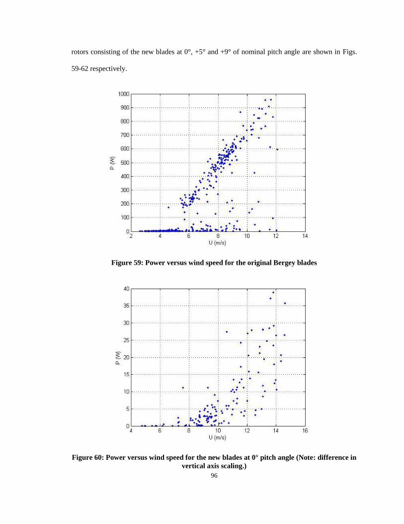
96
rotors consisting of the new blades at 0°, +5° and +9° of nominal pitch angle are shown in Figs.
59-62 respectively.
Figure 59: Power versus wind speed for the original Bergey blades
Figure 60: Power versus wind speed for the new blades at 0° pitch angle (Note: difference in
vertical axis scaling.)
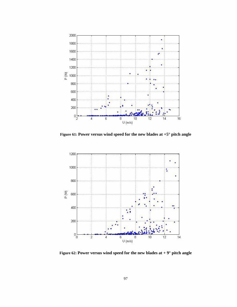
97
Figure 61: Power versus wind speed for the new blades at +5° pitch angle
Figure 62: Power versus wind speed for the new blades at + 9° pitch angle

98
Fig.60 shows that the rotor with the new blades at nominal pitch 0 has a very low maximum
power output of less than 40 W. Further calculation found that most tip speed ratios are less than
3. It is believed the low performance is due to our test system not providing an optimized load for
this turbine. Additionally, the driving distance may not have been long enough to allow the rotor
to reach its design operating point. Due to these factors, the new blades at original pitch (0) were
not included in the analysis that followed.
The data for new rotor with blades at 5° additional pitch angle look sparse though it is enough for
qualitative analysis. On the other hand, in the cases of the original Bergey blades and the new
blades at 9° additional pitch, there are enough data for detailed analysis. It should also be noted
that the original Bergey blades displayed a good consistency with previous trial tests of the
vehicle testing system and the data acquired by Ziter (2010) using conventional fixed tower
method.
7.4.2 Typical road test
The data of one round of road testing for three rotors are shown in Figs. 63-65. It was clear to find
the process of power and rotor speed changed with wind speed. Bergey started soon and furled
easily at wind speed close to 12 m/s; new blades at 5° additional pitch angle started slow and can
reach higher power than the others.
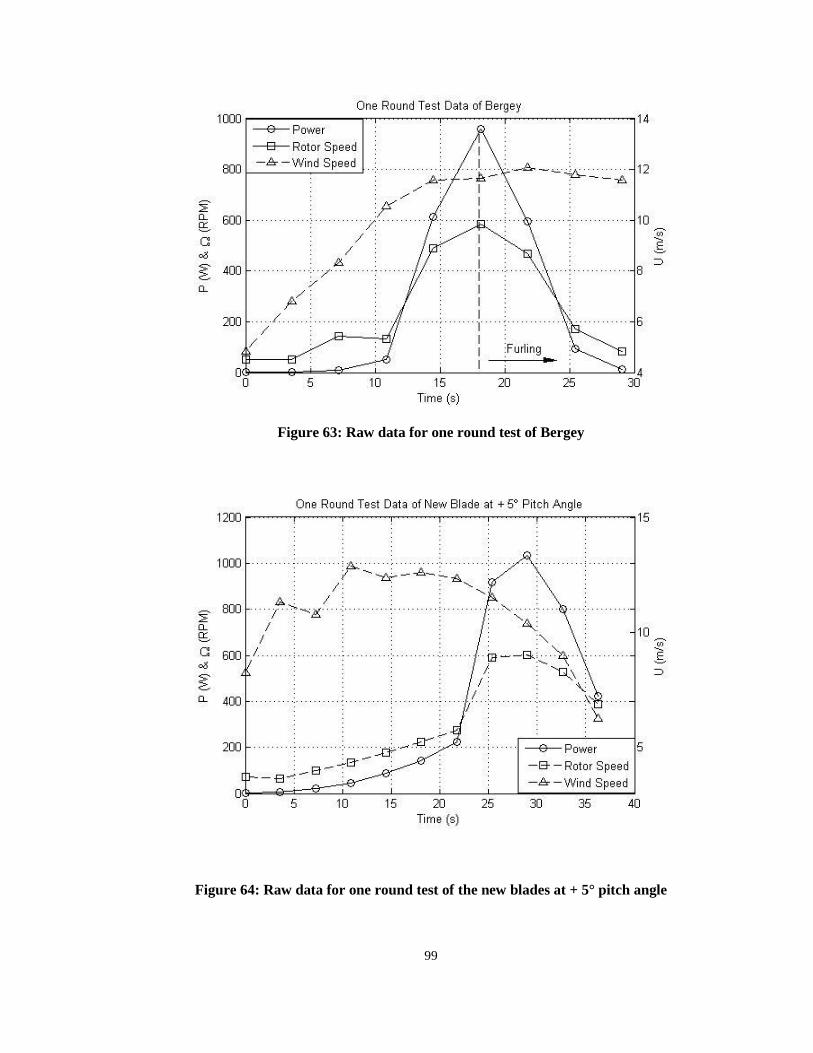
99
Figure 63: Raw data for one round test of Bergey
Figure 64: Raw data for one round test of the new blades at + 5° pitch angle
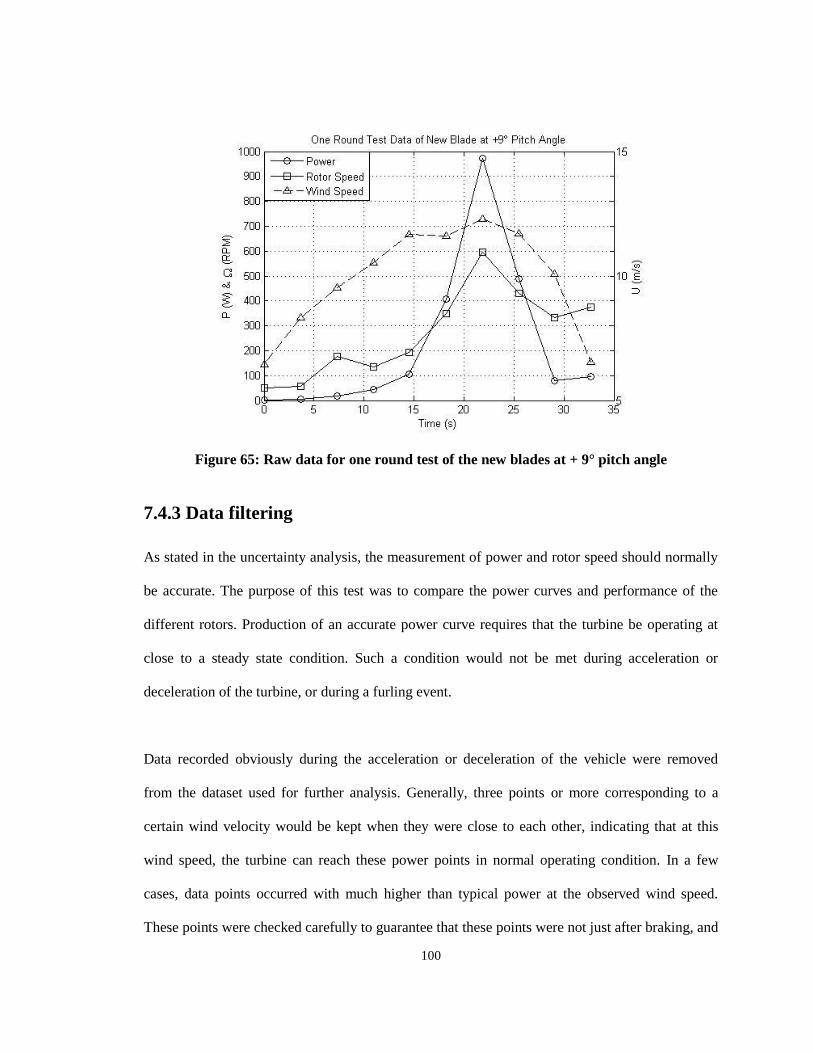
100
Figure 65: Raw data for one round test of the new blades at + 9° pitch angle
7.4.3 Data filtering
As stated in the uncertainty analysis, the measurement of power and rotor speed should normally
be accurate. The purpose of this test was to compare the power curves and performance of the
different rotors. Production of an accurate power curve requires that the turbine be operating at
close to a steady state condition. Such a condition would not be met during acceleration or
deceleration of the turbine, or during a furling event.
Data recorded obviously during the acceleration or deceleration of the vehicle were removed
from the dataset used for further analysis. Generally, three points or more corresponding to a
certain wind velocity would be kept when they were close to each other, indicating that at this
wind speed, the turbine can reach these power points in normal operating condition. In a few
cases, data points occurred with much higher than typical power at the observed wind speed.
These points were checked carefully to guarantee that these points were not just after braking, and

101
deceleration, or just began at the end of a run. The inertia of the rotor may lead to high power
even at low wind speeds if the wind speed decreased rapidly: these points were identified as
outliers and removed. In many cases, the three second average data measured in the test were
lower and far away from the main trend of higher power data points because the turbine was in
acceleration. These points were also removed for they cannot represent the actual power.
During data processing, some rotor speeds in the three-second data were found to be inaccurate,
typically several times greater than would be expected for the measured power output (Power
output and rotor speed are very closely linked for the Bergey XL 1.0). This was traced to errors
that occurred in Labview’s frequency identification that could occur if the period of rotations (or
put another way, the exact time between consecutive pulses in the rotation signal) varied over the
three second averaging period. In some cases, aliasing occurred when a single dominant
frequency was not identified, and the resulting reported frequency for the three second average
was usually a multiple of the true value. Though the three-second average data can be manually
quality controlled to identify these instances as given in Appendix C, these data were not included
in later analysis to improve the reliability and to decrease the possible uncertainty of the raw data.
7.5. Comparison of rotors
Based on rough calculation and the principles of data filtering, the effective data were processed
and compared although not all uncertainties and cofounding variables can be eliminated
completely.
7.5.1 Power curve
After data filtering, revised power curves were calculated, plotted and fitted for the Bergey
blades, and the new blades at +5 and +9 pitch angle respectively (Figs.66-68). The resulting
power curves are shown in Fig.69. Polynomial fits are included, noting that a linear fit works well

102
for the Bergey rotor, and both +5 and +9 use second order fitted curves. The rotor at 5°
additional pitch angle produces the highest power at high wind speeds (over 9 m/s), while the
rotor at 9° additional pitch angle produces the lowest power overall, but has the best performance
at low wind speed. At wind speed of 5 m/s to 9 m/s, the power outputs of all three rotors are
close.
Among all the filtered data, the maximum power signal voltage recorded by the DAQ (VDAQ) is
9.295 V (corresponding to a power of 1889 W) from the rotor with the new blade at 5° additional
pitch angle: in this case the uncertainty is 0.0026 V. The maximum uncertainty of power is
±1.06 W. The lowest VDAQ in the filtered data is 1.934 V (corresponding to 81.8 W power) from
rotor of new blade at 9° additional pitch giving a power uncertainty of ±0.14 W. The uncertainty
from the power calculation is very low compared to the magnitudes of the measured power over
the full range of the data.
Figure 66: Power curve of Bergey blade
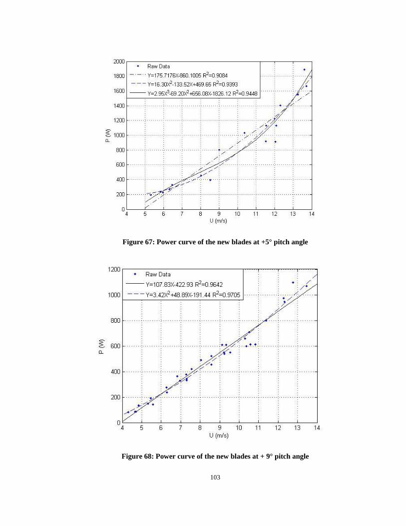
103
Figure 67: Power curve of the new blades at +5° pitch angle
Figure 68: Power curve of the new blades at + 9° pitch angle

104
Figure 69: Power curve comparison of three rotors
7.5.2 Wind speed vs. rotor speed
Since during the test, a constant 2.01 load was used. It was found that rotor speed as a function
of wind velocity, as shown in Fig. 70, are relatively consistent with power versus wind velocity
for all three rotors.
7.5.3 Rotor speed vs. power
The Bergey XL 1.0 generator is a permanent magnet alternator that is directly connected to the
rotor shaft. Using a 2.01 resistor as the electrical load means the electrical load is very
consistent during turbine operation. The power output of the turbine would therefore be expected
to be a consistent function of shaft rotation speed. The filtered data from all rotors tested were
combined to produce the plot of power versus rotation speed shown in Fig.71. This data
confirmed that there is a fixed relationship (the fitted equation) between power and rotor speed in
this test, which further proved the test data are consistent.

105
Figure 70: Rotor speed vs. wind velocity of three rotors
Figure 71: Power vs. rotor speed for three rotors

106
7.5.4 Tip speed ratio
Tip speed ratios versus wind velocity for the three rotors are shown in Figs. 72-74, as well as the
average and the uncertainty of each point. The binned values were the average value of all data
points in the range of wind speed U ± 0.25 m/s and the related mean of tip speed ratios. U was
initialized as 4 m/s or 5 m/s, and then increased by steps of 0.5 m/s up to the maximum observed
speed. However, this approach was used to illustrate the rough trend, and not intended as a
detailed statistical analysis. The uncertainty and average of tip speed ratios are summarized in
Table 5.
Table 5: Uncertainty and mean of tip speed ratio
Rotors Mean of λ Uncertainty of λ
Maximum Minimum
Bergey 6.54 ±0.1304 ±0.0773
+ 5° New rotor 6.96 ± 0.126 ±0.0785
+ 9° New rotor 6.11 ±0.124 ±0.0734
Although the amount of data were not enough to get solid conclusions and a general trend for
each rotor, it was clear that new rotor at +5° pitch angle has the highest tip speed ratio and new
rotor at +9° has the lowest.
Figure 72: Tip speed ratio vs. wind velocity for Bergey
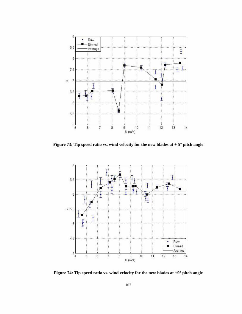
107
Figure 73: Tip speed ratio vs. wind velocity for the new blades at + 5° pitch angle
Figure 74: Tip speed ratio vs. wind velocity for the new blades at +9° pitch angle

108
7.5.5 Power coefficients
As stated in Section 7.3, power coefficients for the three rotors and uncertainties were calculated
and plotted in Figs.75-77. The Bergey blades has the highest average gross power coefficient and
new rotor at 9° additional pitch angle has the lowest average gross power coefficient. It should be
noted that this power coefficient was calculated by output power from generator, not directly
calculated from rotor. After the system efficiency (mainly generator efficiency) from Martinez et
al. (Chapter 4) were taken into account, the average aerodynamic power coefficients were
different from gross power coefficients, as shown in Table 6. The average aerodynamic power
coefficient of +5° rotor is the highest, closely followed by the Bergey. However, because
Martinez et al. did not provide the efficiency data of rotor speed over 500 RPM, the lowest
efficiency of 0.59 at 500 RPM had to be adopted for power coefficient calculation when the rotor
speeds were higher than 500 RPM. These calculations worked as reference of performance
comparisons among three rotors, not for accurate evaluation due to lack of accurate generator
efficiency data in this test.
Table 6: CP summary of three rotors
Rotors Mean of
gross CP
Uncertainty of gross CP Mean of
Aerodynamic CP Max. Min
Bergey 0.296 ±0.026 ±0.0065 0.414
+ 5° New rotor 0.282 ±0.0253 ±0. 0066 0.417
+ 9° New rotor 0.263 ±0.0246 ±0. 0052 0.352
From these figures, it was found that some data were probably affected by deceleration because
gross power coefficients are around 0.4 in Fig.75 and one point over 0.4 in Fig.76. In common
sense, gross power coefficient should be less than 0.4 for small wind turbines. However, overall
data are reasonable compared to previous conventional measurements made using this turbine on
a fixed tower (Ziter, 2010).

109
Figure 75: Power coefficient vs. wind velocity for Bergey
Figure 76: Power coefficient vs. wind velocity for the new blades at + 5° pitch angle
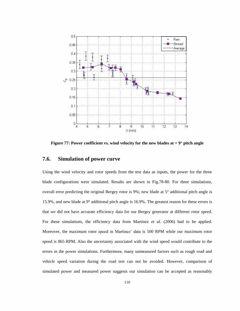
110
Figure 77: Power coefficient vs. wind velocity for the new blades at + 9° pitch angle
7.6. Simulation of power curve
Using the wind velocity and rotor speeds from the test data as inputs, the power for the three
blade configurations were simulated. Results are shown in Fig.78-80. For three simulations,
overall error predicting the original Bergey rotor is 9%; new blade at 5° additional pitch angle is
15.9%, and new blade at 9° additional pitch angle is 16.9%. The greatest reason for these errors is
that we did not have accurate efficiency data for our Bergey generator at different rotor speed.
For these simulations, the efficiency data from Martinez et al. (2006) had to be applied.
Moreover, the maximum rotor speed in Martinez’ data is 500 RPM while our maximum rotor
speed is 865 RPM. Also the uncertainty associated with the wind speed would contribute to the
errors in the power simulations. Furthermore, many unmeasured factors such as rough road and
vehicle speed variation during the road test can not be avoided. However, comparison of
simulated power and measured power suggests our simulation can be accepted as reasonably
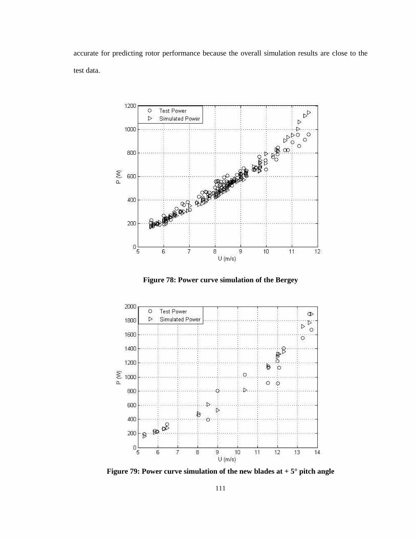
111
accurate for predicting rotor performance because the overall simulation results are close to the
test data.
Figure 78: Power curve simulation of the Bergey
Figure 79: Power curve simulation of the new blades at + 5° pitch angle

112
Figure 80: Power curve simulation of the new blades at + 9° pitch angle
7.7. Discussion
The new blade mounted at the original pitch angle to the hub did not work in the view point of
power generation because the maximum power was 40 W. However, this did not mean
aerodynamic calculation of the blade was wrong. Qualitatively, the new rotor took a very long
time to increase rotation speed, and during testing it rarely operated at designed tip speed ratio.
This issue was magnified by the limited duration of testing possible at higher wind speeds, caused
by the short length of the test road. When the pitch angle was changed to 5° degree, a maximum
power output of 1889 W was reached. To an extent, the new rotor design is unlikely to be as well
matched to the generator as the original Bergey rotor, because the original rotor and the generator
were designed together by the Bergey company (Bergey, 2012).
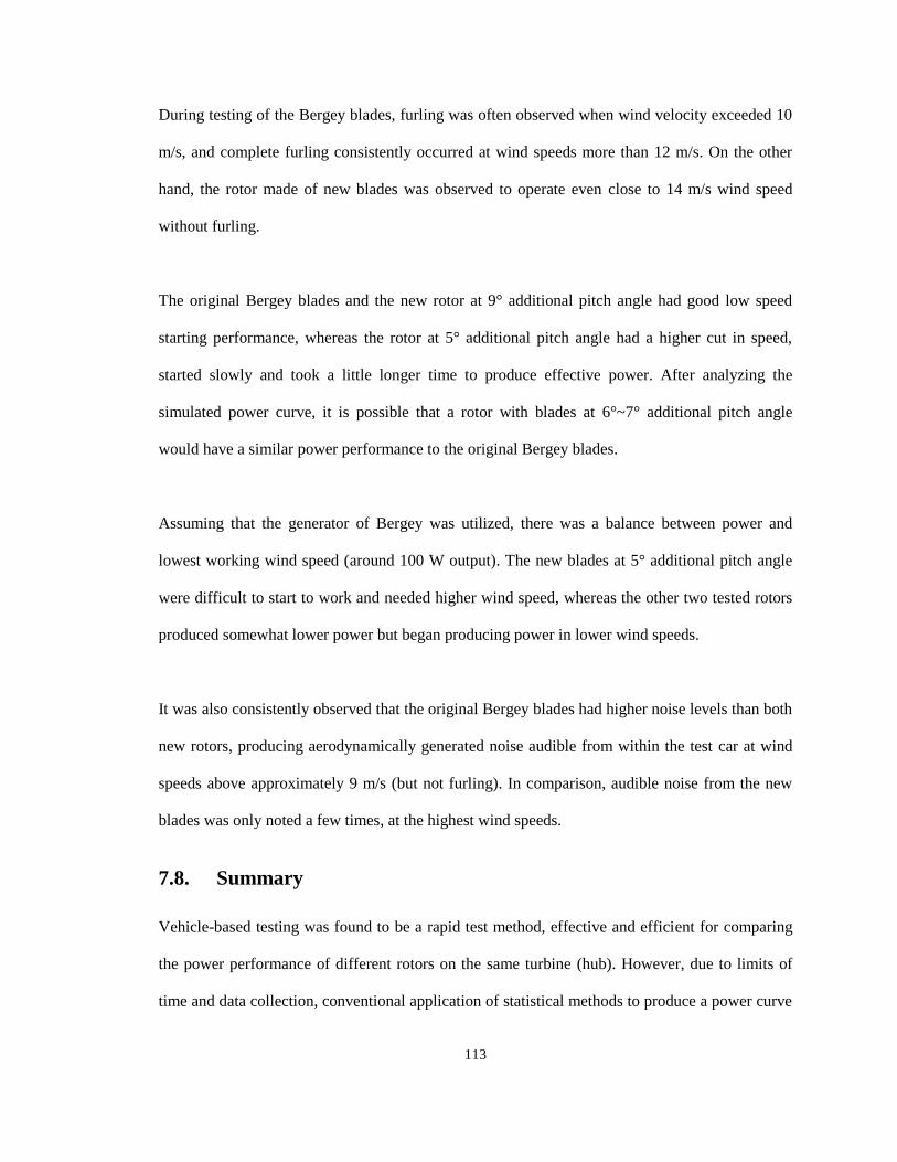
113
During testing of the Bergey blades, furling was often observed when wind velocity exceeded 10
m/s, and complete furling consistently occurred at wind speeds more than 12 m/s. On the other
hand, the rotor made of new blades was observed to operate even close to 14 m/s wind speed
without furling.
The original Bergey blades and the new rotor at 9° additional pitch angle had good low speed
starting performance, whereas the rotor at 5° additional pitch angle had a higher cut in speed,
started slowly and took a little longer time to produce effective power. After analyzing the
simulated power curve, it is possible that a rotor with blades at 6°~7° additional pitch angle
would have a similar power performance to the original Bergey blades.
Assuming that the generator of Bergey was utilized, there was a balance between power and
lowest working wind speed (around 100 W output). The new blades at 5° additional pitch angle
were difficult to start to work and needed higher wind speed, whereas the other two tested rotors
produced somewhat lower power but began producing power in lower wind speeds.
It was also consistently observed that the original Bergey blades had higher noise levels than both
new rotors, producing aerodynamically generated noise audible from within the test car at wind
speeds above approximately 9 m/s (but not furling). In comparison, audible noise from the new
blades was only noted a few times, at the highest wind speeds.
7.8. Summary
Vehicle-based testing was found to be a rapid test method, effective and efficient for comparing
the power performance of different rotors on the same turbine (hub). However, due to limits of
time and data collection, conventional application of statistical methods to produce a power curve

114
is not possible. Careful filtering of measured data to include only quasi-steady observations
allows the production of power curves with a reasonable degree of accuracy to compare
significant design changes such as the impact of a new rotors design. However, the method does
introduce additional uncertainties due to transient conditions and flow induced by the test
vehicles that make it difficult to fully eliminate the uncertainty from the test method itself.
Among three rotors tested, the rotor composed of new blades at 5° additional pitch angle
produces the highest power. The rotor at 9° additional pitch angle has the lowest overall power
output, while the original Bergey rotor has the highest average gross power coefficient. However,
after generator efficiency are taken into account, the rotor at 5° additional pitch angle reaches a
slightly higher power coefficient than the other rotors, which is in accordance with the simulation
curves.
When load is constant, there is a fixed relationship between rotor speed and power in this turbine
system, meaning the rotor with higher aerodynamic performance will have higher rotation speed
at the same wind speed.
Overall, the rotor at 5° additional pitch angle operates at a higher tip speed ratio, with a mean tip
speed ratio close to 7, whereas the Bergey’s mean observed tip speed ratio is 6.5, and rotor at 9°
additional pitch angle has a mean observed tip speed ratio of 6.1. Furthermore, the rotor at 5°
additional pitch angle usually performs well at high wind speeds (over 10 m/s) whereas Bergey
works better at wind speed less than 10 m/s. The rotor at 9° pitch angle has a wide operating
range from 4.5 m/s to 14 m/s, but the lowest power output of the tested rotors.

115
The simulation code works well for the original Bergey blades with average error of 9% and the
new blade designs are simulated with an average error of less than 17%. Based on these results,
the simulation code is good enough for performance prediction.

116
Chapter 8. Summary and conclusions
In this study, a new blade installed on the hub of Bergey XL 1.0 was designed and analyzed with
BEM method, fabricated using an RTM system with epoxy and fibre glass composite, and tested
in a vehicle-based testing system. The new blades had higher aerodynamic performance than
original Bergey XL 1.0 rotor.
The modified BEM power performance simulation code was validated using field test data.
Validation was also conducted with road test data of the original Bergey blade and new blades at
5° and 9° additional pitch angle installation. Tip loss, drag coefficient correction, and wake factor
were taken into account.
Power coefficient predictions were also examined by including or omitting some factors. It was
found that tip loss and drag coefficient cannot be neglected for small wind turbines even though
these factors are negligible for large wind turbines.
Calculation of wake factor using Buhl method produced more reasonable results than Glauert’s or
Wilson-Walker’s although the difference among three methods did not have a great range.
The characteristics of the airfoil beyond the stall point were calculated by flat plate theory and the
Vitena equations. Flat plate theory was the simpler of the two to implement, but the Vitena
method provided smoother transition at the stall point and improved convergence during
numerical simulation.

117
Comparisons of aerodynamic performance in three types of blade geometries produced a design
for a new blade with an SD 7062 airfoil. The power performance of this new rotor at different
additional pitch angles was predicted using BEM methods, then compared with performance
predictions of the original Bergey XL 1.0 rotor.
A multi-purpose aluminum mould was designed and analyzed in stress and displacement with
FEM. Three new design blades of fibre glass and epoxy composites were produced using an
RTM system built at the University of Guelph.
The original Bergey XL 1.0 rotor and new rotors at with blades installed at 5° and 9° additional
pitch angles were successfully tested using vehicle-based testing system. Vehicle-based testing
was found to be a rapid and effective method for quick evaluation of rotor performance,
especially for comparisons among different blades installed on the same hub. The test results
provided sufficient accuracy for evaluation of power performance.
The new rotor at 5° additional pitch angle produces more power than the other two at wind speeds
greater than 10 m/s with higher tip speed ratios. The new rotor at 9° additional pitch angle works
in the widest range of wind speeds from 4.5 m/s to 14 m/s. The original Bergey XL 1.0 rotor
produces more power than the other rotor types at wind speeds less than 10 m/s.
The average gross power coefficients are 0.296, 0.282 and 0.263 for the original Bergey rotor, the
5° and 9° additional pitch angle rotors respectively. After generator efficiency is considered, the
average power coefficients are 0.414 for Bergey, 0.417 for +5° new rotor and 0.352 for +9° new
rotor.

118
Chapter 9. Recommendations
Based on the theoretical analysis and road test, future works are recommended as below.
The original new blades (without additional pitch angle) should be further investigated to
determine how closely they can match with the Bergey XL 1.0 generator, and
consideration should be given to adjusting the electrical load to improve starting
performance.
The furling mechanism should be studied further because the original Bergey XL 1.0
rotor always furled completely at wind speeds close to 12 m/s whereas the new rotor
almost never furled in the test, even at wind speeds approaching 14 m/s.
Methods of balancing the need for a wide range of working wind speed and high power
performance need additional study. For example, the new rotor at 9° additional pitch
angle can produce relatively lower power but over a wide range of wind speed, while the
new rotor with 5° additional pitch angle works well but only at high speed.
In the BEM simulation, the Bergey blade at high tip speed ratios (over 7) was found to
have negative local power coefficients at some locations close to the blade tip, which
meant that part of the blade was working like a propeller and consuming energy rather
than extracting it from the flow. This situation should be examined using CFD.

119
The load and thrust on the small wind turbine blade should be more fully simulated and
tested in a wind tunnel because the original Bergey blades were observed to be obviously
bent after the four-month field test in 2010.
New bio-materials for blade fabrication including natural fibres and/or bio-resin should
be tested to determine if they will work in the RTM system, and to determine optimum
methods to use for forming bio-materials into wind turbine blade structures.
The vehicle test method should be studied by comparing the test data from the vehicle
test to field and wind tunnels of one identical wind turbine. This comparison will allow
the effectiveness of road test to be evaluated and improved.

120
References
Akesson, D., Skrifvars, M., Seppala, J.V., and Walkenstrom, P., “Preparation of Natural Fibre
Composites from Biobased Thermoset Resins,” Proceedings of the 27th Risø International
Symposium On Materials Science: Polymer Composite Materials For Wind Power Turbines,
2006.
AWEA, “AWEA Small Wind Global Market Study 2010,” American Wind Energy Association
[report], 2010.
Audierne, E., Elizondo, J., Bergami L., Ibarra H., Probst, O., “Analysis of the Furling Behavior
of Small Wind Turbines,” Applied Energy, 2010, Vol. 87, pp. 2278-2292.
Balat, M., “A Review of Modern Wind Turbine Technology,” Energy Sources, Part A, 31:1561–
1572, 2009.
Bergey, “Begey XL 1.0 Specifications,” URL: http://www.bergey.com/pages/bergey_xl1.html
[cited March 3, 2011].
Bergey, “BWC EXCEL 1 24 VDC Battery Charging System Owners Manual,” V. 2.3, Bergey
Windpower Co., 2012.
Boer, Ryan Sietze De, “Development of Epoxidized Soybean Oil and Soy Fibre Composites With
Polyhedral Oligomeric Silsesquioxane(Poss) Nano Reinforcement,” Master Thesis, University of
Guelph, 2010.
121
Brøndsted, P., Lilholt, H., and Lystrup, A., “Composite Materials and Wind Power Turbine
Blades,” Annu. Rev. Mater. Res. 2005.35:505-38.
Buhl, Jr.M., “A New Empirical Relationship Between Thrust Coefficient and Induction Factor for
the Turbulent Windmill State,” NREL/TP-500-36834[report], National Renewable Energy
Laboratory(NREL), 2005.
Burton, T., Sharp, D., Jenkins, N., and Bossanyi, E., Wind Energy Handbook, John Wiley & Sons
Ltd, Toronto, 2001.
Clausen, P.D., and Wood, D.H., “Recent Advances in Small Wind Turbine Technology,” Wind
Engineering, Vol. 24, No. 3, 2000, pp. 189-201.
Clifton-Smith, M. J., “Wind Turbine Blade Optimisation with Tip Loss Corrections,” Wind
Engineering, Vol. 33, No. 5, 2009, pp. 477–496.
Clifton-Smith, M. J., “Aerodynamic Noise Reduction for Small Wind Turbine Rotors,” Wind
Engineering, Vol. 34, No. 4, 2010, pp 403–420.
Clifton-Smith, M. J., and Wood, D.H., “Further Dual Purpose Evolutionary Optimization of
Small Wind Turbine Blades,” Journal of Physics: Conference Series 75, 2007, 012017.
Compositesworld, “The Markets Renewable Energy,” URL:
http://www.compositesworld.com/articles/the-markets-renewable-energy-2012 [cited February
24, 2012].

122
Dai, J.C., Hu, Y.P., Liu, D.S., and Long, X., “Aerodynamic Loads Calculation and Analysis for
Large Scale Wind Turbine Based on Combing BEM Modified Theory With Dynamic Stall
Model,” Renewable Energy, Vol. 36, 2011, pp. 1095-1104.
Drela, Mark, “Xfoil 6.96 (Win32)”, http://web.mit.edu/drela/Public/web/xfoil/, May 3, 2006.
Drela, Mark, “Xfoil Manual,” URL: http://web.mit.edu/drela/Public/web/xfoil/xfoil_doc.txt,
2001.
Duquette, M.M. and Visser, K.D., “Numerical Implication of Solidity and Blade Number on
Rotor Performance of Horizontal-Axis Wind Turbines,” Journal of Solar Energy Engineering,
Vol. 125, November 2003, PP 425-432.
Environment Canada, URL:
http://www.climate.weatheroffice.gc.ca/climateData/hourlydata_e.html?StationID=45407&timefr
ame=1&Month=2&Year=2012&cmdB2=Go&Day=2 [cited March 6, 2012].
Frohnapfel, P., Muggenhamer, M., Schlögl, and Drechsler, K., “Natural Fibre Composites for
Innovative Small Scale Wind Turbine Blades,” Technische Universität München [report],
Germany, November 16, 2010.
Giguere, P., and Selig, M.S., “New Airfoils for Small Horizontal Axis Wind Turbines,” Journal
of Solar Energy Engineering, Vol. 120, May 1998, pp108-114.

123
Habali, S.M., and Saleh I.A., “ Local Design, Testing And Manufacturing Of Small Mixed Airfoil
Wind Turbine Blades Of Glass Fibre Reinforced Plastics Part I: Design of The Blade and Root,”
Energy Conversion & management, Vol. 41, 2000, pp. 249-280.
Hansen, Martin O.L., Aerodynamics of Wind Turbines, 2nd ed., Earthscan in the UK and USA,
2008, Chaps, 1-10.
Holmes, J.W., Brøndsted, P., Sørensen, B.F., Sun, Z., and Chen, X., “Development of a Bamboo-
Based Composite as a Sustainable Green Material for Wind Turbine Blades,” Wind Engineering,
Vol. 33, No. 2, 2009, pp. 197-210.
Humiston, C., and Visser, K., “Full Scale Aerodynamic Effects of Solidity and Blade Number on
Small Horizontal Axis Wind Turbines,” World Wind Energy Conference, November 2003.
Johansen, J., Madsen, A., Gaunaa, M., and Bak, C., “Design of a wind Turbine Rotor for
Maximum Aerodynamic Efficiency,” Wind Energy, 2009, 12:261-273.
Kim, T., Lee, S.,eungmin, Kim H., and Lee S., “Design Of Low Noise Airfoil With High
Aerodynamic Performance For Use on Small Wind Turbines,” Science China Technological
Sciences, Vol. 53 No.1, January 2010, pp75-79.
Lanzafame, R., and Messina, M., “Design and Performance of a Double-pitch Wind Turbine with
Non-twisted Blades,” Renewable Energy, Vol. 34, 2009, pp. 1413-1420.

124
Lanzafame, R., and Messina, M., “Fluid Dynamics Wind Turbine Design: Critical Analysis,
Optimization and Application of BEM Theory,” Renewable Energy, Vol. 32, 2007, pp. 2291-
2305.
Larsen, K., “Recycling wind blades,” URL: http://www.wind-watch.org/documents/recycling-
wind-blades/[Cited June 13, 2011].
Leftheriotis, G., and Carpenter, C.J., “ Investigation of Reynolds Number effects on the design of
a Delta wing vortex wind turbine,” Wind Engineering, Vol. 15, No. 1, August 1991, pp8-15.
Lira, I., Evaluating The Measurement Uncertainty: Fundamentals And Practical Guidance,
Institute of Physics Publishing, Bristol, UK, 2002.
Maalawi, K.Y., and Badr, M.A., “A Practical Approach For Selecting Optimum Wind Rotors,”
Renewable Energy, 28, 2003, pp. 803-822.
Mandell, J.F., Samborsky, D.D., Wang, L., and Wahl, N.K., “New Fatigue Data for Wind
Turbine Blade Materials,” Journal of Solar Energy Engineering, Vol. 125, November 2003, pp
506-514.
Martinez, J., Morales, A., Probst, O., Llamas A., and Rodriguez, C., “Analysis and Simulation of
a Wind-electric Battery Charging System,” International Journal of Energy Research, Vol. 30,
2006, pp.633-646.

125
Martinez, J., Bernabini, L., Probst, O., and Rodriguez, C., “ An Improved BEM Model for the
Power Curve Prediction of Stall-regulated Wind Turbines,” Wind Energy, Vol. 8, 2005, pp. 385-
402.
Matsumiya, H., Ito, R., Kawakami, M., Matsushita, D., Lida, M., and Arakawa, C., “Field
Operation and Track Tests of 1-kW Small Wind Turbine under High Wind Conditions,” Journal
of Solar Energy Engineering, Vol. 32, February 2010, pp.11002-11010.
National Instruments, “NI USB-621x Specifications,” April, 2009.
Nichita, C., Mokadem, M.E. and Dakyo, B., “Wind Turbine Simulation Procedures,” Wind
Engineering, Vol. 30, No. 3, 2006, pp. 187-200.
Nottingham Innovative Manufacturing Research Centre (NIMRC), “Natural fibres for new
sustainable products,” URL:
http://www.nottingham.ac.uk/nimrc/documents/pdfsanddocs/naturalfibresfornewsustainableprodu
cts.pdf, [cited in July 15, 2011].
NRGsystems, “NRG 40C Specifications”, URL:
http://www.nrgsystems.com/sitecore/content/Products/1900.aspx?pf=StandardSensors, [cite
February 24, 2012].
NRG, “#40C anemometer uncertainty,” September 23, 2011.

126
NREL, “Definition of Small Wind Turbine,” URL: http://www.nrel.gov/wind/smallwind/, [cited
in February 15, 2012].
Oerlemans, S., Schepers,J.G., Guidati ,G., and Wagner, S., “Experimental demonstration of wind
turbine noise reduction through optimized airfoil shape and trailing-edge serrations,” National
Aerospace Laboratory[Netherlands], NLR-TP-2001-324[report], 2001.
Potter, K., Resin Transfer Moulding, Chapman & Hall, London, U.K., 1997
Peterson, P., and Clausen, P.D., “Timber Of High Efficiency Small Wind Turbine Blades,” Wind
Engineering, Vol. 28, No.1, 2004, pp 87-96.
Refan, Maryam, “Aerodynamic Performance of a Small Horizontal Axis Wind Turbine,” Master
thesis, the University of Western Ontario, 2009.
Rosato, D.V., and Rosato,D.V., Reinforced Plastics Handbook, 3rd
ed., Elsevier Ltd., New York,
USA, 2004.
Scibor-Rylski, A.J., Road Vehicle Aerodynamics, Pentech Press Ltd., London, U.K., 1975.
Seitzler, M., and Kamisky, R., “Small Wind Energy Demonstration System: Installation and
Instrumentation Report,” California Wind Energy Collaborative, University of California, Davis,
2008.

127
Selig, M.S., and McGranahan, B.D.,“Wind Tunnel Aerodynamic Tests of Six Airfoils for Use on
Small Wind Turbines,” Journal of Solar Energy Engineering, Vol. 126, Nov. 2004, pp986-1001.
Sharma, R.N. and Madawala, U., “The Concept of a Smart Wind Turbine System”, 16th
Australasian Fluid Mechanics Conference Crown Plaza, December, 2007, pp. 481-486.
Shen, W.Z., Mikkelsen, R.F., Sørensen, J.N., and Bak, C., “Tip Loss Corrections for Wind
Turbine Computations,” Wind Energy, 8(4): 457-475, 2005.
Southwest windpower, “Air_X Specifications,”
URL: http://www.windenergy.com/sites/all/files/3-CMLT-1339-01_Rev_E_Air_X_Spec.pdf,
2008.
Spera, D.A, Wind Turbine Technology, ASME Press, New York, 1994.
Strong, A.B., Fundamentals of Composites Manufacturing: Materials, Methods, and
Applications, Society of Manufacturing Engineers, Dearborn, Michigan, 1989.
Tangler, J.L., and Kocurek, J.D., “Wind Turbine Post-stall Airfoil Performance Characteristics
Guidelines for Blade Element Momentum Methods,” NREL/CP-500-36900, October 2004.
Tangler, J.L., “The Evolution of Rotor and Blade Design,” NREL/CP-500-28410, July 2000.
Thygesen, A., Thomsen, A.B., Daniel, G., and Lilholt, H., “Comparison Of Hemp Fibres With
Glass Fibres For Wind Power Turbines; Effect Of Composite Density,” Proceedings of the 27th

128
Risø International Symposium On Materials Science: Polymer Composite Materials For Wind
Power Turbines, 2006, pp 329-336.
UIUC, “Summary of Low-Speed Airfoil Data - Vol 3, ” URL: http://www.ae.illinois.edu/m-
selig/pd.html[ cited February 27, 2011].
Veers, P.S., Ashwill, T.D., Sutherland, H.J., Laird, D.L. and Lotitz, D.W., Griffin, D., Mandell,
J.F., Musial, W.D., Jackson, K., Zuteck, M., Miravete, A., Tsai, S.W., and Richmond, J.L.,
“Trends in the Design, Manufacture and Evaluation of Wind Turbine Blades,” Wind Energy, Vol.
6, 2003, pp. 245-259.
WindPowerProgram, “Power Curve,” URL: http://www.wind-power-
program.com/turbine_characteristics.htm, [cited February 15, 2012].
Wright, A.K., and Wood, D.H., “The Starting And Low Wind Speed Behaviour Of A Small
Horizontal Axis Wind Turbine,” Journal of Wind Engineering and Industrial Aerodynamics, Vol.
92, 2004, pp. 1265-1279.
Wood, D.H., “Dual Purpose Design of Small Wind Turbine Blades,” Wind Engineering, Vol. 28,
No. 5, 2004, pp 511-528.
WWEA,
http://www.wwindea.org/home/index.php?option=com_content&task=view&id=345&Itemid=43,
World Wind Energy Association, [cited February 15, 2012].

129
Ziter, Brett, “Alternative Methods of Estimating Hub-height Wind Speed for Small Wind Turbine
Performance Evaluation”, Master Thesis, University of Guelph, May 2010.

130
Appendix A: Aerodynamic parameters of the new blade
Table A: Detailed aerodynamic parameters of the designed blade
r/R r (mm) Chord
(mm)
Section pitch
angle (º)
Thickness
(mm) Airfoil
0.032 40 102 10 Over 14 Mixed airfoil
0.104 130 102 10 Over 14 Mixed airfoil
0.112 140 105 11 14.7 sd7062
0.12 150 108 12 15.12 sd7062
0.16 200 125.2 15.02 17.528 sd7062
0.2 250 121.73 13.97 17.0422 sd7062
0.24 300 118.25 12.54 16.555 sd7062
0.28 350 114.77 11.06 16.0678 sd7062
0.32 400 111.29 9.66 15.5806 sd7062
0.36 450 107.81 8.39 15.0934 sd7062
0.4 500 104.34 7.25 14.6076 sd7062
0.44 550 100.86 6.24 14.1204 sd7062
0.48 600 97.38 5.35 13.6332 sd7062
0.52 650 93.9 4.55 13.146 sd7062
0.56 700 90.42 3.85 12.6588 sd7062
0.6 750 86.95 3.21 12.173 sd7062
0.64 800 83.47 2.65 11.6858 sd7062
0.68 850 79.99 2.14 11.1986 sd7062
0.72 900 76.51 1.67 10.7114 sd7062
0.76 950 73.04 1.25 10.2256 sd7062
0.8 1000 69.56 0.87 9.7384 sd7062
0.84 1050 66.08 0.52 9.2512 sd7062
0.88 1100 62.6 0.2 8.764 sd7062
0.92 1150 59.12 -0.1 8.2768 sd7062
0.96 1200 55.65 -0.37 7.791 sd7062
1 1250 52.17 -0.62 7.3038 sd7062

131
Appendix B: Anemometer verification
Cup anemometer and ultrasonic anemometer were verified in the week just after the road test was
completed. Since both anemometers were calibrated by manufacturers with higher standard than
that can be achieved at the University of Guelph. The test at boundary layer wind tunnel at
University of Guelph was to verify that both anemometers worked well and not damaged
accidentally.
Three positions around pitot tube were chosen to check cup anemometer NRG C40. All data at
different positions are very close and are put together as shown in Fig.B-1. The ultrasonic
anemometer RM Young 8100 was put 3 meters in front of Pitot tube. The data is shown in Fig.B-
2. It was easily to judge that both anemometers worked consistently with respect to Pitot tube.
Figure B-1: Cup anemometer verification

132
Figure B-2: Ultrasonic anemometer verification
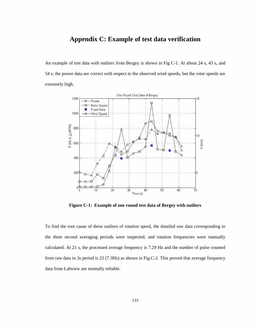
133
Appendix C: Example of test data verification
An example of test data with outliers from Bergey is shown in Fig C-1. At about 24 s, 43 s, and
54 s, the power data are correct with respect to the observed wind speeds, but the rotor speeds are
extremely high.
Figure C-1: Example of one round test data of Bergey with outliers
To find the root cause of these outliers of rotation speed, the detailed raw data corresponding to
the three second averaging periods were inspected, and rotation frequencies were manually
calculated. At 21 s, the processed average frequency is 7.29 Hz and the number of pulse counted
from raw data in 3s period is 22 (7.3Hz) as shown in Fig.C-2. This proved that average frequency
data from Labview are normally reliable.
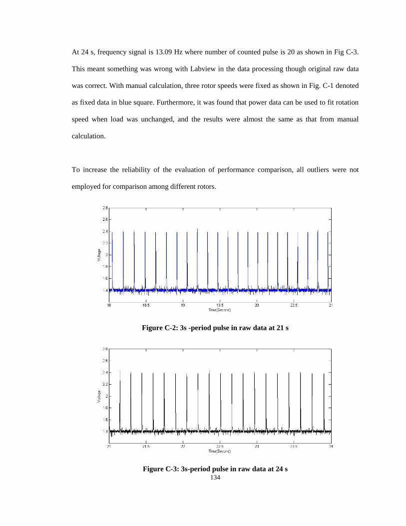
134
At 24 s, frequency signal is 13.09 Hz where number of counted pulse is 20 as shown in Fig C-3.
This meant something was wrong with Labview in the data processing though original raw data
was correct. With manual calculation, three rotor speeds were fixed as shown in Fig. C-1 denoted
as fixed data in blue square. Furthermore, it was found that power data can be used to fit rotation
speed when load was unchanged, and the results were almost the same as that from manual
calculation.
To increase the reliability of the evaluation of performance comparison, all outliers were not
employed for comparison among different rotors.
Figure C-2: 3s -period pulse in raw data at 21 s
Figure C-3: 3s-period pulse in raw data at 24 s