design, development, and human analogous control...

DESIGN, DEVELOPMENT, AND HUMAN ANALOGOUS

CONTROL OF A CLIMBING ROBOT

A Thesis

Submitted to the Faculty of Graduate Studies and Research

In Partial Fulfillment of the Requirements

For the Degree of

Master of Applied Science

In

Industrial Systems Engineering

University of Regina

By

Amirhossein Bazargan

Regina, Saskatchewan

March 2012

©Copyright 2012: Amirhossein Bazargan

UNIVERSITY OF REGINA

FACULTY OF GRADUATE STUDIES AND RESEARCH

SUPERVISORY AND EXAMINING COMMITTEE

Amirhossein Bazargan, candidate for the degree of Master of Applied Science in Industrial Systems Engineering, has presented a thesis titled, Design, Development, and Human Analogous Control of a Climbing Robot, in an oral examination held on February 3, 2012. The following committee members have found the thesis acceptable in form and content, and that the candidate demonstrated satisfactory knowledge of the subject material. External Examiner: Dr. Raman Paranjape, Electronic Systems Engineering

Co-Supervisor: Dr. Mehran Mehrandezh, Industrial Systems Engineering

Co-Supervisor: Dr. Liming Dai, Industrial Systems Engineering

Committee Member: Dr. Adisorn Aroonwilas, Industrial Systems Engineering

Committee Member: Dr. Rene Mayorga, Industrial Systems Engineering

Chair of Defense: Dr. Daryl Hepting, Department of Computer Science *Not present at defense

i

Abstract

In this thesis, a re-configurable wheeled climbing robot has been introduced. This robot is

capable of doing a multitude of tasks that no other single robot could do in the past. It can

climb staircases, move inside empty ducts and pipes, climb up ropes and poles of varying

cross sections, and even jump over obstacles with proper motion coordination. It can also

move inside narrow passageways by reconfiguring itself. The design of a re-configurable

robot capable of traversing a wide range of unconventional terrains is the novelty in this

invention.

A comprehensive dynamic model of the robot is derived for the first time. A real-time

simulator to try different control strategies by a human operator using conventional

human-machine interfaces has been developed. This simulator can be employed to size

the electromechanical actuators and to synthesize different control strategies in a short

time. The data obtained can be also used to design a human-analogous autonomous

controller.

ii

After outline of the theory, background and applications of soft computing techniques for

system construction and control including Artificial Neural Networks (ANN), Fuzzy

Logic Control (FLC), and the Adaptive Neuro-Fuzzy Inference Systems (ANFIS), a

novel human-analogous control strategy based on ANFIS was implemented to control the

position of the robot climbing a straight pole against gravity.

The design process of the ANFIS-based human-analogous control strategy includes the

following steps: First, a human expert tries to control the real system in real time within a

human-in-the-loop simulator via a Human-Machine Interface (HMI) using sensory

information obtained from visual tracing in the HMI in real time from the real system.

The control task is done by using a control interface (i.e., a joystick). Relevant

input/output data is stored, filtered, and used offline to tune the parameters of an ANFIS-

based controller. The ANFIS controller whose parameters have been optimized is then

implemented on the real system autonomously. Based on the information obtained via the

HITL simulator system, the controller can extrapolate needed data for untrained cases.

iii

Acknowledgements

I would like to express my thanks and appreciation to my thesis supervisor Dr. Mehran

Mehrandezh and co-supervisor Dr. Liming Dai for being so enthusiastic, cooperative

and helpful and for financial supports during the development of this dissertation. I would

also like to express my thanks and appreciation to the Faculty of Graduate Studies and

Research (FGSR) and the Faculty of Engineering and Applied Science at University of

Regina in form of teaching and research scholarships.

iv

Dedication

I would like to dedicate this thesis to my parents, Ebrahim and Soosan, and my wife,

Delbar, for always supporting me in every situation and believing in me even when I was

unsure of myself.

v

Contents

Abstract i

Acknowledgement iii

Dedication iv

Table of Contents v

List of Tables ix

List of Figures xi

List of Acronyms xv

Chapter 1 Introduction 1

1.1 Problem Statement . . . . . . . . . . . . . . . . . . . . . . . . . . . . . . . . . . . . . . . . . . . . . 1

1.2 Thesis Organization . . . . . . . . . . . . . . . . . . . . . . . . . . . . . . . . . . . . . . . . . . . . 2

1.3 Contribution . . . . . . . . . . . . . . . . . . . . . . . . . . . . . . . . . . . . . . . . . . . . . . . . . . 2

Chapter 2 Literature review 4

2.1 Re-configurable and adaptable vehicles . . . . . . . . . . . . . . . . . . . . . . . . . . . . . 4

2.1.1 Obstacle/stair climber robots . . . . . . . . . . . . . . . . . . . . . . . . . . . . . . . . . . 5

vi

2.1.2 Rope/pole/wall climbing robots . . . . . . . . . . . . . . . . . . . . . . . . . . . . . . . . 7

2.1.3 Pipe/duct rovers . . . . . . . . . . . . . . . . . . . . . . . . . . . . . . . . . . . . . . . . . . . . 9

2.2 Control of vehicles . . . . . . . . . . . . . . . . . . . . . . . . . . . . . . . . . . . . . . . . . . . . . 11

Chapter 3 Problem Definition 12

3.1 Design and Development . . . . . . . . . . . . . . . . . . . . . . . . . . . . . . . . . . . . . . . . 13

3.1.1 Simplicity . . . . . . . . . . . . . . . . . . . . . . . . . . . . . . . . . . . . . . . . . . . . . . . . 13

3.1.2 Versatility . . . . . . . . . . . . . . . . . . . . . . . . . . . . . . . . . . . . . . . . . . . . . . . . 13

3.1.3 Speed . . . . . . . . . . . . . . . . . . . . . . . . . . . . . . . . . . . . . . . . . . . . . . . . . . . 18

3.1.4 Easy control . . . . . . . . . . . . . . . . . . . . . . . . . . . . . . . . . . . . . . . . . . . . . . 18

3.2 Control . . . . . . . . . . . . . . . . . . . . . . . . . . . . . . . . . . . . . . . . . . . . . . . . . . . . . . 21

Chapter 4 The Electro-Mechanical Design and the Mechanistic Model of the

Proposed Robot

22

4.1 Robot Design . . . . . . . . . . . . . . . . . . . . . . . . . . . . . . . . . . . . . . . . . . . . . . . . . 22

4.2 Mechanistic Model . . . . . . . . . . . . . . . . . . . . . . . . . . . . . . . . . . . . . . . . . . . . . 26

4.3 Dynamic Equations . . . . . . . . . . . . . . . . . . . . . . . . . . . . . . . . . . . . . . . . . . . 29

4.4 Applied Forces . . . . . . . . . . . . . . . . . . . . . . . . . . . . . . . . . . . . . . . . . . . . . . . . 31

4.4.1 Friction Forces . . . . . . . . . . . . . . . . . . . . . . . . . . . . . . . . . . . . . . . . . . . . 31

4.4.2 Normal Forces . . . . . . . . . . . . . . . . . . . . . . . . . . . . . . . . . . . . . . . . . . . . 32

4.4.3 Applied Torque of Geared DC Motors . . . . . . . . . . . . . . . . . . . . . . . . . 35

4.5 Summary . . . . . . . . . . . . . . . . . . . . . . . . . . . . . . . . . . . . . . . . . . . . . . . . . . . . 35

Chapter 5 Human Analogous Control 39

5.1 Background . . . . . . . . . . . . . . . . . . . . . . . . . . . . . . . . . . . . . . . . . . . . . . . . . . . 40

5.1.1 Fuzzy Controllers . . . . . . . . . . . . . . . . . . . . . . . . . . . . . . . . . . . . . . . . . 40

vii

5.1.2 Artificial Neural Network . . . . . . . . . . . . . . . . . . . . . . . . . . . . . . . . . . . 42

5.1.3 Adaptive Networks . . . . . . . . . . . . . . . . . . . . . . . . . . . . . . . . . . . . . . . . 45

5.1.4 Adaptive Neuro-Fuzzy Inference Systems . . . . . . . . . . . . . . . . . . . . . . 47

5.2 Fuzzy Logic Controller . . . . . . . . . . . . . . . . . . . . . . . . . . . . . . . . . . . . . . . . . . 49

5.2.1 Structure of Fuzzy Logic Controller . . . . . . . . . . . . . . . . . . . . . . . . . . . 49

5.2.2 Real-time Human-in-the-loop Simulator . . . . . . . . . . . . . . . . . . . . . . . . 50

5.2.3 Selection of Training Data . . . . . . . . . . . . . . . . . . . . . . . . . . . . . . . . . . . 57

5.2.3.1 Consistency . . . . . . . . . . . . . . . . . . . . . . . . . . . . . . . . . . . . . . . . . . 58

5.2.3.2 Tracing Reference Trajectory . . . . . . . . . . . . . . . . . . . . . . . . . . . . 65

5.2.4 Training Data Preparation . . . . . . . . . . . . . . . . . . . . . . . . . . . . . . . . . . . 66

5.2.5 Tuning the FLC . . . . . . . . . . . . . . . . . . . . . . . . . . . . . . . . . . . . . . . . . . . 70

5.2.6 Simulation Result . . . . . . . . . . . . . . . . . . . . . . . . . . . . . . . . . . . . . . . . . 76

5.2.7 Real-time Experiment . . . . . . . . . . . . . . . . . . . . . . . . . . . . . . . . . . . . . . 77

5.3 PID Controller . . . . . . . . . . . . . . . . . . . . . . . . . . . . . . . . . . . . . . . . . . . . . . . . 80

5.4 Discussion . . . . . . . . . . . . . . . . . . . . . . . . . . . . . . . . . . . . . . . . . . . . . . . . . . . . 83

5.4.1 FLC vs. PID Controller . . . . . . . . . . . . . . . . . . . . . . . . . . . . . . . . . . . . . 83

5.4.2 Effects of Improving Training Data . . . . . . . . . . . . . . . . . . . . . . . . . . . 84

Chapter 6 Conclusion and Future Work 86

6.1 Conclusion . . . . . . . . . . . . . . . . . . . . . . . . . . . . . . . . . . . . . . . . . . . . . . . . . . . 86

6.2 Future Work . . . . . . . . . . . . . . . . . . . . . . . . . . . . . . . . . . . . . . . . . . . . . . . . . . 87

Bibliography 89

Appendix A Simulink Model of the Climbing Robot 96

Appendix B Case study: Control of Rotating Angle of a DC motor 98

viii

B.1 Dynamic Equations . . . . . . . . . . . . . . . . . . . . . . . . . . . . . . . . . . . . . . . . . . . . . . 98

B.2 Conventional Controller . . . . . . . . . . . . . . . . . . . . . . . . . . . . . . . . . . . . . . . . . . . 100

B.3 Unconventional Controller . . . . . . . . . . . . . . . . . . . . . . . . . . . . . . . . . . . . . . . . . 102

B.4 Comparing Conventional and Unconventional Controllers . . . . . . . . . . . . . . . . 111

Appendix C Basic Definitions 112

ix

List of Tables

3.1 Comparison of design factors for some robots cited in the Literature . . . . . . 19

4.1 Definition of physical parameters used in equation 4.13 . . . . . . . . . . . . . . . . 37

4.2 Constant values used in simulink model . . . . . . . . . . . . . . . . . . . . . . . . . . . . 38

5.1 Correlation coefficient of five different results . . . . . . . . . . . . . . . . . . . . . . . 65

5.2 Average Tp , average Ts , and percentage of overshoot for each result . . . . . 66

5.3 An example of improving some pair data . . . . . . . . . . . . . . . . . . . . . . . . . . . 68

5.4 Antecedent parameters before tuning . . . . . . . . . . . . . . . . . . . . . . . . . . . . . . . 73

5.5 Antecedent parameters after tuning . . . . . . . . . . . . . . . . . . . . . . . . . . . . . . . . 74

5.6 Consequent parameters after tuning . . . . . . . . . . . . . . . . . . . . . . . . . . . . . . . . 75

5.7 Effect of independent P and D tuning [48] . . . . . . . . . . . . . . . . . . . . . . . . . . 81

B.1

Parameters of the DC motor used in the case study presented in appendix B

. . . . . . . . . . . . . . . . . . . . . . . . . . . . . . . . . . . . . . . . . . . . . . . . . . . . . . . . . . . . .

100

B.2

Antecedent parameters before tuning for case study of controlling the

rotation angle of a DC motor . . . . . . . . . . . . . . . . . . . . . . . . . . . . . . . . . . . . .

107

x

B.3

Antecedent parameters after tuning for case study of controlling the


108

B.4

Consequent parameters after tuning for case study of controlling the


109

xi

List of Figures

3.1 Curved pole climbing application domain . . . . . . . . . . . . . . . . . . . . . . . . . 14

3.2 Rope climbing application domain . . . . . . . . . . . . . . . . . . . . . . . . . . . . . . . 14

3.3 Stair climbing application domain . . . . . . . . . . . . . . . . . . . . . . . . . . . . . . . 15

3.4 Duct climbing application domain . . . . . . . . . . . . . . . . . . . . . . . . . . . . . . . 15

3.5 Duct climbing application domain with varying ross section . . . . . . . . . . 16

3.6 Rough-terrain rover application domain . . . . . . . . . . . . . . . . . . . . . . . . . . 16

3.7 Pipe-crawling application domain . . . . . . . . . . . . . . . . . . . . . . . . . . . . . . . 17

3.8 Moving through difficult passageways . . . . . . . . . . . . . . . . . . . . . . . . . . . 17

3.9 Payload application domain . . . . . . . . . . . . . . . . . . . . . . . . . . . . . . . . . . . 18

3.10 Flowchart of the design process . . . . . . . . . . . . . . . . . . . . . . . . . . . . . . . . 20

4.1 (a) Main parts of the robot (b) General view . . . . . . . . . . . . . . . . . . . . . . . 23

4.2 Technical drawing of the robot . . . . . . . . . . . . . . . . . . . . . . . . . . . . . . . . . . 25

4.3 Generalized coordinates of the system . . . . . . . . . . . . . . . . . . . . . . . . . . . . 28

4.4 Applied forces on the robot . . . . . . . . . . . . . . . . . . . . . . . . . . . . . . . . . . . . 32

xii

4.5 Modeling the pole as a spring damper . . . . . . . . . . . . . . . . . . . . . . . . . . . . 34

5.1 A snapshot of the HMI . . . . . . . . . . . . . . . . . . . . . . . . . . . . . . . . . . . . . . . . 51

5.2 Reference trajectory . . . . . . . . . . . . . . . . . . . . . . . . . . . . . . . . . . . . . . . . . . 52

5.3

Result No.1 including desired and real value of vertical movement, input

voltage, and error . . . . . . . . . . . . . . . . . . . . . . . . . . . . . . . . . . . . . . . . . . . .

53

5.4



54

5.5



55

5.6



56

5.7



57

5.8 Change of voltage in terms of error for four steps of result No.1 . . . . . . . 60





5.13 Filtered voltage used to tune the ANFIS . . . . . . . . . . . . . . . . . . . . . . . . . . 69

5.14 Filtered error used to tune the ANFIS . . . . . . . . . . . . . . . . . . . . . . . . . . . . 69

5.15 The Gaussian MF’s of e(k) before tuning . . . . . . . . . . . . . . . . . . . . . . . . . 71

5.16 The Gaussian MF’s of e(k) after tuning . . . . . . . . . . . . . . . . . . . . . . . . . . . 71

5.17 The Gaussian MF’s of e(k-1) before tuning . . . . . . . . . . . . . . . . . . . . . . . . 72

xiii

5.18 The Gaussian MF’s of e(k-1) after tuning . . . . . . . . . . . . . . . . . . . . . . . . . 72

5.19 The control surface . . . . . . . . . . . . . . . . . . . . . . . . . . . . . . . . . . . . . . . . . . . 72

5.20 Implementation of an ANFIS controller in the closed-loop . . . . . . . . . . . . 76

5.21 Tracing the reference trajectory using ANFIS . . . . . . . . . . . . . . . . . . . . . . 76

5.22 Response of the ANFIS controller . . . . . . . . . . . . . . . . . . . . . . . . . . . . . . . 77

5.23 A snapshot of the physical apparatus . . . . . . . . . . . . . . . . . . . . . . . . . . . . . 78

5.24

Tracing the reference trajectory using an ANFIS controller in an

experimental test . . . . . . . . . . . . . . . . . . . . . . . . . . . . . . . . . . . . . . . . . . . . .

79

5.25 Response of an ANFIS controller in an experimental test . . . . . . . . . . . . . 79

5.26 Tracing a reference trajectory using a PID controller . . . . . . . . . . . . . . . . 82

5.27 Response of the PID controller . . . . . . . . . . . . . . . . . . . . . . . . . . . . . . . . . . 83

5.28

Tracing the reference trajectory using the ANFIS controller which is

tuned by all pair data . . . . . . . . . . . . . . . . . . . . . . . . . . . . . . . . . . . . . . . . . .

85

A.1 Simulink model of the system . . . . . . . . . . . . . . . . . . . . . . . . . . . . . . . . . . 97

B.1 Simulink model of a DC motor . . . . . . . . . . . . . . . . . . . . . . . . . . . . . . . . . 99

B.2

Implementation of a PID controller in the closed-loop for controlling the

rotation angle of a DC motor . . . . . . . . . . . . . . . . . . . . . . . . . . . . . . . . . . .

100

B.3 Output of the PID controller to control the rotating angle of a DC motor . 101

B.4 Rotation angle of a DC motor using a PID controller . . . . . . . . . . . . . . . . 102

B.5

Membership function of input1 before tuning for the case study of

controlling the rotation angle of a DC motor . . . . . . . . . . . . . . . . . . . . . . .

104

B.6

Membership function of input1 after tuning for the case study of


104

xiv

B.7

Membership function of input2 before tuning for the case study of


105

B.8

Membership function of input2 after tuning for the case study of


105

B.9

Control surface of the FLC for the case study of controlling the rotation

angle of a DC motor . . . . . . . . . . . . . . . . . . . . . . . . . . . . . . . . . . . . . . . . . .

106

B.10

Response of the fuzzy logic controller for the case study of controlling

the rotation angle of a DC motor . . . . . . . . . . . . . . . . . . . . . . . . . . . . . . . .

110

B.11

Rotation angle of a DC motor using a fuzzy logic controller for the case

study of controlling the rotation angle of a DC motor. . . . . . . . . . . . . . . . .

110

C.1 A Feedforward Adaptive Network . . . . . . . . . . . . . . . . . . . . . . . . . . . . . . . 114

C.2 A Recurrent Network . . . . . . . . . . . . . . . . . . . . . . . . . . . . . . . . . . . . . . . . . 115

C.3 Topological Ordering Representation . . . . . . . . . . . . . . . . . . . . . . . . . . . . 116

C.4 Triangle (x;20,50,80) membership function . . . . . . . . . . . . . . . . . . . . . . . . 117

C.5 Trapezoid (x;10,20,50,80) membership function . . . . . . . . . . . . . . . . . . . . 118

C.6 Gaussian (x;50,15) membership function . . . . . . . . . . . . . . . . . . . . . . . . . . 119

C.7 Bell (x;25,3,50) membership function . . . . . . . . . . . . . . . . . . . . . . . . . . . . 119

C.8 Sig (x;0.2,50) membership function . . . . . . . . . . . . . . . . . . . . . . . . . . . . . . 120

C.9

(a) A two-input first-order Sugeno fuzzy model with two rules, (b)

Equivalent ANFIS Architecture . . . . . . . . . . . . . . . . . . . . . . . . . . . . . . . . .

124

C.10 ANFIS structure with two inputs . . . . . . . . . . . . . . . . . . . . . . . . . . . . . . . . 126

xv

List of Acronyms

The following acronyms are used frequently in this report with these meanings:

DOF : Degrees Of Freedom

FLC : Fuzzy logic Controller

PID : Proportional Integral Derivative

ANN : Artificial Neural Network

FIS : Fuzzy Inference System

TSK : Takagi-Sugeno-Kang

HITL : Human In The Loop

SHFC : Supervisory Hierarchical Fuzzy Controller

ANFIS : Adaptive Neuro-Fuzzy Inference System

xvi

IEEE : Institute of Electrical and Electronics Engineers

ODE : Ordinary Differential Equation

1

Chapter 1

Introduction

1.1 Problem Statement

The problems investigated in this thesis are firstly, the design and dynamic analysis of a

climbing robot and secondly, the design and implementation of an optimal stand-alone

fuzzy logic controller (FLC) to control the movement of the robot. Using an Adaptive

Neuro-Fuzzy Inference System (ANFIS), the controller parameters (antecedents and the

consequents of the rules) can be tuned offline based on information obtained through a

Human-in-the-Loop (HITL) simulator. An operator tries to do the control task via this

simulator using the visual feedback sensory information provided to him/her via a Human

Machine Interface (HMI). In order to tune the ANFIS parameters, the numerical

input/output information taken from the HITL simulator has been used.

2

Using ANFIS we can find out the optimal values for the mentioned parameters so that the

system produces the best match between the input/output of the system and those

obtained from HITL. This unconventional controller is a human-analogous controller

and has less complexity rather than a conventional model-based controller.

1.2 Thesis Organization

This thesis is organized as follows: Chapter 2 provides a literature review of different

kind of robots specifically climbing robots and a short review about controllers. Chapter

3 deals with problem definition. Chapter 4 presents the design and dynamic analysis of

the climbing robot. Chapters 5 presents the simulation and experimental results for the

control of vertical position of the climbing robot. Concluding statements and different

possibilities to extend this work are presented in chapter 6.

1.3 Contribution

This thesis introduces a novel design of a climbing robot. The design of a robot capable

of traversing a wide range of unconventional terrains is the novelty of this invention. A

comprehensive dynamic model of the robot is derived for the first time. To control the

robot an Adaptive Neuro-Fuzzy Inference System (ANFIS) based controller is used. To

tune the parameters of this ANFIS a novel approach using input/output data captured

from a human-in-the-loop simulator was used. In this method a human controls the

system using a joystick based on visually-provided sensory feedback through an HMI

unit. In previous research the parameters of ANFIS or Fuzzy Logic Controller FLC were

tuned using linguistic information feedback from the human operators. The shortcoming

3

of this method is the inherent limitation of detail in verbal and written communication. In

other words, the description of a person’s insight about the controls can differ from

person to person. This can cause some confusion in tuning and effect the performance of

the controller.

For this thesis, the numerical input/output data captured directly from the manual control

by an operator with a human-in-the-loop simulator is fed directly into the ANFIS to tune

its parameters. Through simulation and experimentation the results of control using the

ANFIS are shown in this thesis.

4

Chapter 2

Literature Review

2.1 Re-configurable and Adaptable Vehicles

Automation benefits society in several ways. For example, automating tasks by using a

machine instead of a person to perform dangerous tasks can reduce the likelihood that a

person will be injured while performing the tasks. It can also increase productivity by

performing the tasks faster than a human could. Design and development of re-

configurable and adaptable vehicles that can travel over unconventional terrain has been

carried out for the past three decades. Generally, these robotic systems can be

categorized as wheeled robots [e.g. 1-3], crawlers [e.g. 2], and hopping machines [e.g. 3].

While one single machine may be able to traverse a number of difficult terrains, there is

no single machine that can handle them all. For instance, the Starcly robot developed by

Le et al. can climb staircases and obstacles, but it cannot climb up poles/ropes [4]. As

5

another example, the robot developed by Xu et al. can climb up poles within a narrow

range of size and unchanging cross section shape [1]. Further modifications would be

required to make it move over curved poles.

Climber robots can be categorized as (1) wheeled, and (2) legged robots. In

wheeled robots the wheels maintain their contacts with the surface they are climbing on

all the time [e.g. 1]. However, in legged robots, only a subset of legs will be touching the

surface [5]. Most of the legged robots also need to re-configure themselves to match the

task. Normally, the climber robots use adhesion. This adhesive force could be

electromagnetic or vacuum suction, [e.g. 6-8]. The electromagnetic ones can traverse

only ferrous material while pneumatic ones can only climb smooth surfaces. Our robot

can be categorized as a re-configurable wheeled machine that maintains its contact with

the surface it is climbing on at all times.

The proposed robotic system was targeted for use on a large variety of terrains

without compromising its agility or unnecessarily increasing the complexity of its design.

A brief literature survey on the state-of-the-art of low-degree-of-freedom (low-dof)

climber robots moving on different terrains is given below. These robots are classified by

the terrains they move on as: (1) obstacle climbing robots, (2) rope/pole/wall climbing

robots, and (3) pipe/duct rovers.

2.1.1 Obstacle/stair Climber Robots:

These robots are designed to climb over obstacles found in rough terrains. One of the

most difficult cases would be to climb up a staircase. There are some lab-scale and

commercial robots available that can do this task repeatedly with a high success rate.

6

However, these robots can climb neither confined spaces such as ducts or pipes, nor can

they climb ropes/poles. Some systems cited in literature are addressed below in more

detail.

Starcly Robot: Starcly robot has been designed for both climbing and descending

stairs. This robot benefits from the advantage of using treads and robotic arm linkages

simultaneously. Starcly has two arms and two treads on each side. The treads provide

the motive power for the vehicle when it is not climbing stairs and/or obstacles while

the arms move the robot up and down on stairs. Each arm consists of five links which

lift the robot up and down stairs. The arms can also be used as grippers to clear or

remove unwanted obstacles encountered by the robot. There are three idle wheels

attached to each arm to reduce friction when the arm touches the ground during

operation [4]. Although the Starcly robot can navigate obstacles and stairs, it is not

able to navigate in ducts, pipes or up and down poles/ropes.

Stair climbing robot: This robot consists of a main body with a roller chain for

movement on flat surfaces and a front and back arm for climbing and descending

stairs. This robot is equipped with two brushless dc motors, worm gears, two dc

motors to control the two arms and a DSP-based board as the controller. Rubber

blocks are attached to increase friction with the ground and stairs. The direction of

the robot is controlled by varying the speed of the two brushless dc motors [9]. This

robot, like the previous one, cannot climb ropes and poles and cannot navigate pipes

and ducts. On the other hand, this robot is very fast.

7

2.1.2 Rope/pole/wall Climbing Robots:

These robots can be categorized as (1) human-like, and (2) wheeled climbers. The

human-like climbers have many degrees of freedom, therefore the motion coordination

for a smooth climb is a challenging task. Some systems cited in the literature can be

found in [10,11]. The wheeled machines are much simpler in design with fewer degrees

of freedom, and are therefore easier to control. However, they are less versatile compared

to the re-configurable human-like climbers. The robot developed by Nili et al. can, for

instance, climb up straight poles with round cross sections [12]. Some relevant systems

cited in literature are addressed below in more detail.

Sloth Robot: Sloth robot is considered a rope climbing robot. To design this robot,

the anatomy and movement of a real sloth was studied. SLOTH robot consists of

three small servos and is controlled through a SSC II serial servo controller. The

weight of this robot is 250g and its length is 0.2m. The maximum climbing speed of

this robot is 60 meters per hour. Sloth robot can carry a small video camera to offer

"visual access" in places where access by human presence is difficult or dangerous

such as buildings affected by an earthquake or poisonous or toxic environments [13].

The advantages of this robot are its simplicity and cost, but it cannot move over flat

surfaces or in ducts and pipes.

Stickybot: Stickybot is a climbing robot that can climb smooth vertical surfaces such

as glass, plastic, and ceramic tiles. It can reach a maximum speed of 4cm/s. Studying

the anatomy and movement of a gecko inspired Stickybot's mechanical design and its

8

climbing gaits. In the design of this robot, a hierarchy of compliant structures,

directional adhesion, and control of tangential contact forces to achieve control of

adhesion were considered. The undersides of Stickybot's toes are covered with small

stalks which adhere when pulled tangentially from the tips of the toes toward the

ankles. When these stalks are pulled in the opposite direction, they release. A force

control strategy is made by working in combination with the compliant structures and

directional adhesion. This strategy balances forces among the feet and promotes

smooth attachment and detachment of the toes, [10]. Stickybot is fast but it cannot

climb stairs, ropes, ducts or pipes.

Dante II: Is a mobile robot with a tether which has been designed for volcano

exploration and inspection. It has six legs, and uses a tether to support itself on steep

terrain like mountaineers using a climbing rope. The tether is connected to a

generator and a satellite communication station which is located at the volcano's rim

[11]. Dante II has the ability to climb obstacles and move on steep surfaces but it

cannot climb ropes and poles.

Wheel-based Cable Climbing: This robot is a wheeled cable climbing robot which is

able to climb up and down vertical cables specifically used on cable-stayed bridges

for inspection. This robot has a hexagonal body composed of two equally spaced

modules which are joined by connecting bars. This robot can climb up a cable with

diameters varying from 65 mm to 205 mm with payloads of up to 3.5 kg. In case of

electric break-down a gas damper with a slider-crank mechanism is used to exhaust

9

the energy generated by gravity as the robot slides down along the cable, resulting in

a safe landing [1]. This robot can climb poles easily but it cannot climb over/inside

pipes and ducts. It also cannot move over surfaces.

2.1.3 Pipe/duct Rovers:

Robots moving against gravity in the confined spaces found in pipes/air ducts fall under

this category. These days, different kinds of remote controlled robots are used for

inspection and servicing pipes in plants and drain pipes. Most of these robots benefit

from drive wheels which are pressed against the wall of the pipe by a spring to generate

the necessary normal force to support the weight of the robot. Some examples of this

type of robot are;

A three-wheeled robot which is able to move along the inside of pipes and ducts

with a wide range of diameters. This robot benefits from a scissor-like set-up

with three wheels, one at the joint and one at the end of the two limbs [14]. This

robot is not able to move over the pipes and ducts. It also cannot climb stairs and

obstacles.

Another example has a stepping mechanism in which one segment of the body is

stuck in the pipe by hydraulic cylinders, while the other is pulled or pushed

forward, [15]. This robot like the previous one cannot climb stairs and obstacles.

It also cannot move over surfaces.

Another approach by A. Madhani and S. Dubowsky [16] uses three legs for

climbing between two ladders which support the weight of robot. The robot’s

control system pre-plans the movements of the robot through the known

10

environment. This robot cannot climb over poles and surfaces.

In another approach by W. Neubauer [17] eight legs were used which are pushed

against the pipe walls to generate the necessary normal force to support the

weight of body. The legs have the ability to step over almost all surface shapes

and enable the robot to move inside considerably complex-shaped hollows. On

the other hand, this robot takes a great deal of energy to move, has a very

complex control system and is not able to climb over poles.

The pipe crawling robot developed by M. Mehrandezh et al. [18] can move

inside pipes of 6 to 8 inch of diameter. Their robot is wheeled. It can negotiate

curved sections of a pipe thanks to it flexible joints. But this robot cannot climb

over ducts, pipes and poles. It also is not able to climb stairs and obstacles.

Research and development continues concerning vehicles that are robust and adaptable to

a task with the ability to respond to changes in their surroundings. The vehicle presented

in this paper can do most of the tasks the aforementioned robots can do. Specifically it

can climb over obstacles, climb up ropes/poles and inside pipes/ducts by re-configuring

itself as necessary. To the best of our knowledge, no single robot exists that can traverse

such a vast range of unconventional terrains. Our robot is also simple in design, easy to

control, easy to setup with minimum manpower needed and very agile. This robot

provides a simple, lightweight, modular and re-configurable platform that can travel over

a large variety of terrain. The number of actuators and/or propulsion units requited to

move the robot is less than that of its counterparts.

11

2.2 Control of Vehicles

All controllers can be divided to two main groups: conventional (i.e. mechanistic) and

unconventional (i.e. intelligent) controllers. In order to design a mechanistic controller, a

mathematical model of the system is needed. This mathematical model presents the

dynamic of the system. Therefore, for complicated systems which have multiple inputs

and multiple outputs, design of conventional controllers is a difficult and time consuming

process. Today, this task has been made easier using computer aided design. Because

low-order linearized models are used in industry, conventional controllers are common.

Proportional-Integral-Derivative (PID) controllers are an example of conventional

controllers which are popular in industry. A disadvantage of conventional controllers is

that their performance is degraded when the operating point is far from the nominal point.

In other words, the best performance of conventional controllers occurs around the

nominal points. Alternatively, when designing unconventional controllers there is no

need for a mathematical model of the system. Consequently, unconventional controllers

are used in a condition of complicity with the dynamics of the system. Furthermore,

unconventional controllers are used in many situations in which a greater degree of

autonomy is required. In other words, unconventional controllers are more flexible

because they incorporate logic, reasoning and heuristics into conventional control theory

[19]. Some essential factors for intelligent control are [20]:

-learning capability

-autonomous behaviour

-adaptive characteristics

12

Chapter 3

Problem Definition

The problem investigated in this thesis is the design, development, and human analogous

control of a new re-configurable vehicle. This vehicle is capable of climbing staircases,

moving inside empty ducts and pipes, climbing up ropes and poles with varying cross

sections, shapes, and sizes and even jumping over obstacles with proper motion

coordination. It can also pass through difficult passageways by reconfiguring itself. All

these abilities make this robot a novel and versatile robot able to perform a wide range of

tasks that no other robot could do in the past. The following paragraphs deal with some

considerations in design, development and control of this robot.

13

3.1 Design and Development of the Climbing Robot

The design of this re-configurable robot which is capable of traversing a wide range of

unconventional terrains is the novelty in this invention. Some of the most important

factors which have been considered in the design of this robot are as follows:

3.1.1 Simplicity

Considering today’s competitive market, it seems imperative to build as simple a robot as

possible with maximum effectiveness. This robot is mechanically very simple and very

cheap since it uses only 6 simple geared DC motors. It is even possible to use 3 geared

DC motors instead of 6 geared DC motors. The following items are some considerations

in the number of geared DC motors to use:

Power/mass ratio: increasing the number of geared DC motors increases the

weight of the robot as well as the power. The plot of power/mass for DC motors is

an exponential curve. In other words, adding a DC motor increases the percentage

of power more than the percentage of mass. In case of using battery to prepare

needed power the weight of each battery should be considered as well.

Symmetry: using 6 geared DC motor instead of 3 helps the robot be more

symmetric. This allows the robot to not need to turn during climbing.

3.1.2 Versatility

Versatility is another design factor of this robot. This robot is one of the most versatile

robots that has been built since it can work with poles and ropes of different sizes,

14

different materials and different stiffness. This robot can also go on curved poles, move

inside ducts and pipes of varying cross-section and pass through difficult passageways.

Furthermore, this robot can be used as a platform for small payloads. Some application

domains of this robot are shown in following schematic figures:

Curved pole climbing

This robot is able to climb over curved poles.

Figure 3.1: Curved pole climbing application domain

Rope climbing

This robot can climb over ropes which are not rigid as shown in Figure 3.2.

Figure 3.2: Rope climbing application domain

15

Stair climbing

This robot can climb up and down stairs.

Figure 3.3: Stair climbing application domain

Duct climbing

Duct climbing is another application domain of this robot.

Figure 3.4: Duct climbing application domain

16

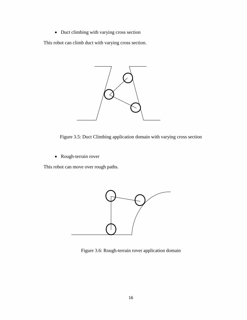
Duct climbing with varying cross section

This robot can climb duct with varying cross section.

Figure 3.5: Duct Climbing application domain with varying cross section

Rough-terrain rover

This robot can move over rough paths.

Figure 3.6: Rough-terrain rover application domain

17

Pipe-crawling robot

As shown in the below figure, this robot can crawl in straight and curved pipes

Figure 3.7: Pipe-crawling application domain

Moving through difficult passageways

Changing its height, this robot can move though difficult passageways as shown in Figure

3.8.

Figure 3.8: Moving through difficult passageways

18

Payloads

Payload cargo is another application domain of this robot. Figure 3.9 deals with this

application domain.

Figure 3.9: Payload application domain

3.1.3 Speed

High speed is another advantage of this robot. Usually in climber robots the act of

catching or holding the rope or pole and moving cannot happen simultaneously, while in

this robot these two acts can happen simultaneously. This fact allows the robot to benefit

from high speed.

3.1.4 Easy Control

All the motions of this robot are based on 3 pair geared DC motors. Low number of

actuators causes this robot to be easily controlled. Most of the robots cited in the

literature benefit more actuators which make their dynamic analysis and control more

19

complicated. In most of the cases, an easier control not only causes a motion more similar

to desired motion but also can decrease the cost of control.

Table 3.1 compares the design factors in some robots cited in the literature. In this table,

the solid circles indicate possession of that design factor.

To dynamically analyze the robot, Lagrangian equations have been used. In chapter 4, a

comprehensive dynamic model of the robot is derived for the first time. The steps of the

design are shown in Figure 3.10.

Type equation here.

Table 3.1 Comparison of the design factors in some robots cited in the literature

Robot Simplicity Versatility Speed Easy control

Stracly robot X √ X X

Stair climbing robot X X √ X

Sloth robot √ X X √

Stickybot √ X √ √

Dante II X √ √ X

Wheel-based climbing robot √ X √ √

Three-wheeled robot √ X √ √

Three-leg robot √ X X √

Pipe crawling robot √ X √ √

Our proposed robot √ √ √ √

20

Figure 3.10: Flowchart of the design process

21

3.2 Control

The design process of the ANFIS-based human-analogous control strategy includes the

following steps:

1) Using a control interface (i.e., a joystick), a human operator attempts to control

the real system in real time via a Human-Machine Interface (HMI). This process

is based on sensory information obtained from visual tracing in the HMI in real

time.

2) The input/output data obtained from step 1 is stored, filtered, and used offline to

tune the parameters of an ANFIS-based controller.

3) The ANFIS controller whose parameters have been optimized in the previous

step is used in a closed-loop on the real system.

22

Chapter 4

The Electro-Mechanical Design and the Mechanistic Model of

the Proposed Robot

In this chapter the design of the climbing robot is introduced and its dynamics are

analyzed. The dynamic equation of the robot is derived from the pole climbing action and

then a Simulink model of the dynamic of the system is presented.

4.1 Robot Design

The robot, in its simplest form, has two extending arms, two sets of active (or powered)

wheels, one set of passive (or idle) wheels, three sets of actuators (i.e., brush-type DC

motors), and a host of onboard sensors (see Figure 4.1a). Two sets of paired motors are

connected to the powered wheels. They are denoted as upper and lower driving motors. A

set of paired motors in the middle, noted as arm-extending motors, is used to extend and

23

retract the arms. The onboard sensors used in the prototype are categorized as intero-

ceptive. This means that they are used to measure the relative movement between

different parts of the robot. The intero-ceptive sensors currently used in the prototype

include optical wheel encoders. They provide angular measurements on all the rotary

axes of the robot. Extero-ceptive sensors such as cameras and Inertial Measurement Units

(IMUs) can be added to the system for external measurements.

(a) (b)

Figure 4.1: (a) Main parts of the robot (b) General view

Figure 4.1b represents the schematic of the robot climbing a pole showing all major

components. The way the robot can be operated is briefly explained here. By extending

the arms using the arm-extending motors one can push against the pole until the friction

force is large enough to support robot’s weight. The upper and lower driving motors can

then be activated to run the robot up and down the pole. One can actively control the arm

Encoder

Powered

wheels

Upper

driving

motors

Lower

driving

motors

Idle wheel

Arm-

extending

motors

Powered

wheels

Pole

Idle wheel

24

extension to negotiate curved sections and poles with varying cross-sections. Closing the

arms beyond a certain threshold will cause a free fall. Extero-ceptive sensors, such as

IMUs, can be used to detect the free fall. The robot should be able to re-grasp the pole it

is climbing very quickly by extending its arms when a free fall is detected.

Figure 4.2 represents the technical drawing of the robot showing all components. The

structure of the robot is briefly explained here. Driving motors (items 1) turn powered

wheels (items 3a) which are connected to them via hubs (items 6a). They make the robot

move up and down along the rope. The bodies of middle motors (items 2) are fixed to the

lower arms (items 5b) via two Motor mounts (Items 10) and two hubs (items 7c), while

their shafts have been fixed to the upper arms (items 5a) via four hubs (2 of item 6b and 2

of item 7b) and two “L” connectors (items 9). When the middle motors turn, the angle

between upper and lower arms changes. The middle motors can open and close the arms,

allowing the robot to grasp a pole tightly when climbing against gravity.

25

Figure 4.2: Technical drawing of the robot

26

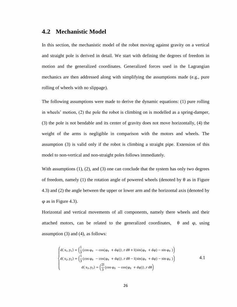
4.2 Mechanistic Model

In this section, the mechanistic model of the robot moving against gravity on a vertical

and straight pole is derived in detail. We start with defining the degrees of freedom in

motion and the generalized coordinates. Generalized forces used in the Lagrangian

mechanics are then addressed along with simplifying the assumptions made (e.g., pure

rolling of wheels with no slippage).

The following assumptions were made to derive the dynamic equations: (1) pure rolling

in wheels’ motion, (2) the pole the robot is climbing on is modelled as a spring-damper,

(3) the pole is not bendable and its center of gravity does not move horizontally, (4) the

weight of the arms is negligible in comparison with the motors and wheels. The

assumption (3) is valid only if the robot is climbing a straight pipe. Extension of this

model to non-vertical and non-straight poles follows immediately.

With assumptions (1), (2), and (3) one can conclude that the system has only two degrees

of freedom, namely (1) the rotation angle of powered wheels (denoted by θ as in Figure

4.3) and (2) the angle between the upper or lower arm and the horizontal axis (denoted by

φ as in Figure 4.3).

Horizontal and vertical movements of all components, namely there wheels and their

attached motors, can be related to the generalized coordinates, θ and φ, using

assumption (3) and (4), as follows:

d x1 , y1 =

l

3(cos φ0 − cos(φ0 + dφ)) , r dθ + l(sin(φ0 + dφ) − sin φ0 )

d x2 , y2 = l

3(cos φ0 − cos(φ0 + dφ)) , r dθ − l(sin(φ0 + dφ) − sin φ0 )

d x3 , y3 = 2l

3(cos φ0 − cos(φ0 + dφ)) , r dθ

4.1

27

Where, in d(xi, yi), i = 1, 2, 3 denoting the incremental and infinitesimal x-y movements

for all point masses seen in Figure 4.3. Also φ0 denotes the initial angle between

upper/lower arms and the horizontal axis when the wheels are just touching the pole’s

surface without exerting any force. The “r” and “l” in Eqn. 4.1 denote the wheels’ radii

and the arms’ length, respectively.

28

(x2,y2)

m2

(x1,y1)

m1

(x3,y3)

m3

Figure 4.3: Generalized Coordinates of the System

X

Y φ

θ

29

With the assumption that cos dφ = 1 and sin dφ = dφ , one can write equations 4.1

as follow:

d x1, y1 =

l

3dφ sin φ0 , r dθ + ldφ cos φ0

d x2, y2 = l

3dφ sin φ0 , r dθ − ldφ cos φ0

d x3, y3 = 2l

3dφ sin φ0 , r dθ

4.2

Correspondingly, the velocities can be calculated as follows:

v1 =

d x1, y1

dt=

l

3φ sin φ0 , rθ + lφ cos φ0

v2 =d x2, y2

dt=

l

3φ sin φ0 , rθ − lφ cos φ0

v3 =d x3, y3

dt=

2l

3φ sin φ0 , rθ

4.3

4.3 Dynamic Equations

Lagrangian mechanics was used to derive the dynamics equations. The Lagrangian

equations based on the two generalized coordinates, θ and φ can be written as:

d

dt ∂T

∂θ −

∂V

∂θ −

∂T

∂θ−

∂V

∂θ = Q θ

d

dt ∂T

∂φ −

∂V

∂φ −

∂T

∂φ−

∂V

∂φ = Q φ

4.4

Where, T and V are Kinetic and Potential energies, respectively and

Q θ and Q φ are non potential parts of the generalized forces in directions θ and φ

respectively.

30

One can therefore write:

T =I1

2 θ + φ

2+

I2

2 θ − φ

2+

I3

2θ 2 +

m1

2 v1 2 +

m2

2 v2 2 +

m3

2 v3 2

V = m1g y1 + m2g y2 + m3g y3

4.5

Where, mi denotes the mass of the ith

part, for i = 1,2,3 (see Figure 4.3). Also the

moments of inertia for the rotary parts and arms can be calculated as:

Ii =1

2miri

2 , i = 1,2,3

Given that m1 = m2 = m3 and that r1 = r2 = r3 , one can simplify equations by using the

notation:

m = m1 = m2 = m3

r = r1 = r2 = r3

I = I1 = I2 = I3

Therefore, Eqn. 4.5 can be simplified to:

T =

9

4mr2θ 2 +

mr2

2+

ml2

3

π

180

2

sin φ0 2 + ml2

π

180

2

cos φ0 2 φ 2

V = 3mrgθ

4.6

Using Eqn. 4.4, the dynamics equations of the system will be:

9

2mr2θ + 3mgr = Q θ

φ mr2 +2ml2

3 sin φ0

2 + 2ml2 cos φ0 2 = Q φ

4.7

31

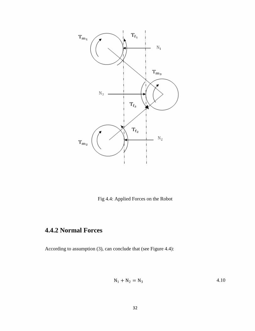
4.4 Applied Forces

As shown in figure 4.4, the applied non potential forces (the right side of equations 4.7)

are:

Q θ = Tm1

+ Tm2− Tf1

− Tf2

Q φ = Tm3− Tf3

4.8

Where, Tmi denotes the torque applied by the ith

pair of the geared DC motors for i = 1,

2, 3. Tfi denotes the resisting torque due to friction between the ith

wheel and the pole

(dry friction), and friction between the shafts of the ith pair of DC motors and their

bearings (viscous friction) for i = 1, 2. Tf3 denotes the resistant torque due to the friction

between the inside plane of the idle wheel and outside plane of the joints of the middle

motors (dry friction) and friction between the shafts of the pair of DC motors and their

bearings (viscous friction). Ni denotes the normal force applied on wheel ith

.

4.4.1 Friction Forces

According to a simple but common model of the friction, the resisting torques due to

dry/viscous frictions can be written as:

Tf1= 2fv1

θ + φ + μr N1 r sign θ + φ

Tf2= 2fv2

θ + φ + μr N2 r sign θ + φ

Tf3= 2 fv3

φ + μra N3 ra sign φ

4.9

Where, fv i is viscous friction coefficient of the i

th geared motor, μr is rolling friction

coefficient between wheels and pole, μra is rolling friction coefficient between inside

area of wheel 3 and its axle, and ra is the radius of the axle of wheel 3.

32

Fig 4.4: Applied Forces on the Robot

4.4.2 Normal Forces

According to assumption (3), can conclude that (see Figure 4.4):

N1 + N2 = N3 4.10

33

Moreover, due to the symmetric shape of the robot one can safely assume N1 = N2. The

following name convention is used from this point on: N = N1 = N2.

By assuming a spring/damper model for the pole (see Figure 4.5), we have:

N3 = 2N = k dx3 + bv3 = k 2l

3(cos φ0 − cos φ) + b

2l

3φ sin φ 4.11

Where k and b denote the stiffness and damping ratios of the pole’s model, respectively.

34

N3

N3

l

l

2φ0

x3

l

l

2φ

Figure 4.5: Modeling the Pole as a Spring Damper

k

b

35

4.4.3 Applied Torque of Geared DC Motors

Considering the dynamics of the DC motors one can relate the input voltage provided to

the motor to its electromechanical torque as follows [21]:

Tm1

= 2ƞ1kt1

u1 − ƞ1kb1θ

R1

Tm2= 2ƞ2kt2

u2 − ƞ2kb2

θ

R2

Tm3= 2ƞ3kt3

u3 − ƞ3kb3

φ

R3

4.12

Where ƞi is gear ratio of the ith

geared DC motor, kti is the torque constant of the i

th DC

motor, ui is the voltage of the ith

DC motor, kb i is the back EMF constant of the i

th DC

motor and Ri is the resistance of the ith

geared DC motor.

4.5 Summary

Referring to equations 4.9 and 4.12, one can rewrite equations 4.8 as:

Q θ = 4ƞ1,2kt1,2

u1,2 − ƞ1,2kb1,2

θ

R1,2 − 2μrN r sign θ + φ − 4fv1,2

θ + φ

Q φ = 2ƞ3kt3

u3 − ƞ3kb3φ

R3 − 2μra N rasign φ − 2fv3

φ

4.13

36

Where,

fv1,2= fv1

= fv2

ƞ1,2 = ƞ1 = ƞ2u1,2 = u1 = u2

kt1,2= kt1

= kt2

kb1,2= kb1

= kb2

Equations 4.7, 4.11 and 4.13 are used to analyze the dynamics of the robot. These

equations also can be used to create a Simulink model of the dynamics of the robot. A

schematic view of this Simulink model is available in Appendix A.

Table 4.1 lists the definitions of physical parameters used in equation 4.13. Table 4.2

deals with the constant values that are used in the Simulink model. Definition of these

constants is in Table 4.1

37

Table 4.1: Definition of physical parameters used in equation 4.13

Physical

Parameter Definition

N Normal force from the cable acting on the wheel 1 and 2

kti Torque constant of the i

th geared motor

kb i Back EMF constant of the i

th geared motor

Ri Resistance of the ith

geared motor’s armature

ƞi Ratio of the ith

motor’s gear box

μra Rolling friction coefficient between the inside area of wheel 3 and

its axle

μr Rolling friction coefficient between the wheels and the pole

ra The axle radius for wheel 3

fv i Viscous friction coefficient of the i

th geared motor

ui Voltage of the ith

geared motor

r Radius of the wheels

l Length of arms

38

Table 4.2: Constant values used in simulink model

Constant Value Unit

R12 2.4 Ohm

R3 2.4 Ohm

b 100 N.s/m

fv12 2e-04 N.m.s

fv3 4e-04 N.m.s

g 9.8 m/s2

K 1500 N/m

Kb12 0.0075 V/rad/s

Kb3 0.0077 V/rad/s

Kt12 0.0075 N.m/A

Kt3 0.0077 N.m/A

L 0.16 M

M 0.325 Kg

Mu 0.4 -

Mur 0.05 -

n12 30 -

n3 50 -

Phi0 44.56 Degree

r 0.027 M

ra 0.006 M

39

Chapter 5

Human Analogous Control

The main objective of this chapter is to design a controller to provide appropriate input

voltages to the climbing robot presented in this thesis to obtain a desired vertical position

of the robot as the output. A desired amount of vertical position change in the form of

step changes was generated in a simulated environment. In general, the robot’s motion

can be regulated by either changing the normal force N exerted on the pole via the robot’s

wheels, changing the angle between the arms, or by changing the input voltage provided

to the driving DC motors. In this thesis, the latter method was adopted as the control

variable while the arm-extention motors provide the needed normal force to support the

weight of the robot. Furthermore, the input voltage of four driving DC motors (upper and

lower DC motors) are equal and therefore their motions are the same.

40

In this chapter, the behaviour of a fuzzy logic controller, trained using an Adaptive

Network-based Fuzzy Inference System (ANFIS) algorithm, is compared with a

Proportional Integral Derivative (PID) controller.

Furthermore, a method to evaluate the human-generated data and a method to increase

the consistency of this data is presented.

All mentioned steps have been applied to control the rotation angle of a simple DC motor

as a case study. The details of this case study are available in Appendix B. Appendix C

deals with some basic definitions which are related to this chapter.

5.1 Background

As the first step, a literature review of the previous works in the area of Fuzzy Logic

Controller, Artificial Neural Network, and Adaptive Neuro- Fuzzy Interface System

(ANFIS) follows:

5.1.1 Fuzzy Controllers

Zadeh [22] introduced and formalized Fuzzy set theory in 1956 and applied it to control

systems in 1973 [23]. Later on, Fuzzy Logic theory was applied to control an ill-modeled

system by Mamdani in 1974 [24]. After that, Fuzzy set theory was employed to solve

different kinds of control problems. As some examples of this, we present the following

items:

A design of a fuzzy logic controller module for a loop controller was proposed by

Ahn, Kim, and Kwon. The speed of a fuzzy logic controller and the number of

parameters to define a fuzzy logic controller were mentioned as the main limitations in

41

implementing the fuzzy logic controller in a loop controller. They used a fixed control

table to increase the inference speed and reduce the number of defining parameters [25].

Bhende, Mishra, and Jain compared the application of a Takagi-Sugeno (TS)-type

fuzzy logic controller, a Mamadani-type fuzzy logic controller and a conventional

Proportional Integral (PI) controller to a three-phase shunt active power filter for the

power-quality improvement and reactive power compensation required by a nonlinear

load. As the first advantage of using fuzzy logic control, they mentioned that this method

did not require a mathematical model of the system. The application of the Mamdani-type

fuzzy logic controller to a three-phase shunt active power filter had the limitation of a

larger number of fuzzy sets and rules. Therefore, it needed to optimize a large number of

coefficients, which increased the complexity of the controller in Mamadani type versus

TS type. On the other hand, they mentioned that “TS fuzzy controllers are quite general

in that they use arbitrary input fuzzy sets, any type of fuzzy logic, and the general

defuzzifier.” Moreover, to implement a TS fuzzy controller a lower number of rules and

classes must be used [26].

Amer, Sallam, and Elawady improved PID-type fuzzy controller performance for

the control of a three DOF rigid planar robot manipulator by implementation of a fuzzy

logic-based pre-compensator followed by a fuzzy self-tuning PID controller.

Proportional-Integral-Derivative (PID)-type fuzzy controllers are the most popular

conventional motion control strategy in industrial use. In the fuzzy self-tuning PID

controller, a Supervisory Hierarchical Fuzzy Controller (SHFC) was used to tune the

inputs of the fuzzy PID controller according to the actual tracking of position error and

velocity error [27].

42

Li and Shen compared the illustration of the fuzzy PD and fuzzy ID and

concluded that the two corresponding fuzzy control rules are similar. Using theoretical

analysis, they showed that the PID fuzzy controller had the feature of non-linearity

besides that of the traditional PID controller. Furthermore, according to simulation

results, they showed that PID fuzzy controller performance was better than that of the

fuzzy PI and the conventional PID controller. [28]

A novel fuzzy logic secondary voltage controller based on a polar fuzzy logic rule

was presented by Lingzhi, Shuangxi, and Qi. The purpose of the presented controller was

adjusting the voltage level of the pilot node by using the voltage of the pilot node as a

feedback signal through an excitation control following the rules of fuzzy logic. The

inputs of the fuzzy controller were the voltage error of pilot nodes and the voltage

differential. The output of the fuzzy controller was the voltage control signal which was

the input of a PI block. The regional voltage control signal was the output of this PI

block. For the New England 39 node system, simulation of a small disturbance on load

shows that the fuzzy logic controller can restore the voltage level faster than conventional

controllers with a larger steady voltage stability margin than conventional secondary

voltage controllers [29].

5.1.2 Artificial Neural Network

Sometimes it is difficult to transcribe human knowledge to fuzzy control rules or define

the parameters of the fuzzy system. In these cases, if sufficient process data is available,

it is possible to benefit from neural networks. Despite the difference between the

43

application requirement of a fuzzy control system and neural networks, they can be used

together. For instance,

Pedrycz and Sosnowski tried to genetically optimize fuzzy decision trees (G-

DTs). “Decision trees are fundamental architectures of machine learning, pattern

recognition, and system modeling”. They developed the fuzzy set-based generalization of

the generic decision tree with discrete or interval-valued attributes by using individual

nodes. These nodes played the role of fuzzy "switches" by distributing the flow of

processing completed within the tree [30].

Keller, Hayashi, and Chen introduce a method to analyze the operation of

individual nodes in a neural network where the nodes implement weighted Yager additive

hybrid operators. “This is because, after training, the neurons can be viewed as mini-rules

which are (primarily) conjunctions, disjunctions, or compensators”. They showed that

using these nodes, satisfying results could be obtained compared to simple cases of fuzzy

logic inference [31].

A study of the synthesis of neural network and fuzzy logic based controllers for

optimally controlling nonlinear applications was presented by Chen, Yang, and Xu. They

presented three different kinds of hierarchical controller architectures which included a

hierarchical neuro-fuzzy controller architecture, a hierarchical fuzzy-neuro controller

architecture and a hierarchical fuzzy logic controller architecture. They showed that the

proposed neural-network and fuzzy logic based control schemes are useful for nonlinear

system applications [32].

In conventional control methods such as Proportional Integral Derivative (PID)

controllers, a mathematical model of the dynamics of the system is required, while in

44

many actual applications, we don’t have an accurate model of the system. In these

conditions, an Artificial Neural Network (ANN) can be useful. Some examples of such

ANN-based controllers are as follows:

Sharof and Lie presented a coordinated excitation/governor ANN-based controller

for AC synchronous generators. The full global action of the voltage regulator, power

system stabilizer, and speed governor controls were modeled by the proposed ANN based

controller [33].

Yao, Wang, and Zhang developed a control scheme of an ANN-based PID

controller to produce high-precision tracking control for an electro-hydraulic servo

system. They used a PID controller to support the stability of the system. They also used

a Cerebellar Model Articulation Controller (CMAC) neural network as a feed-forward

compensator to identify the inverse system dynamics model. The CMAC and the PID

controller were connected and acted in parallel so that the outputs of these paralleled

controllers were summed as the total control action. They also used a Nonlinear Tracking

Differentiator (NTD) to yield high quality differential signals for the PID controller. The

main task of this control algorithm was to minimize the error between the total control

action and the output of the CMAC [34].

An ANN based digital controller for a three phase active power filter was

presented by Sindhu, Nair, and Nambiar. “Three-phase shunt active power filters are

designed to effectively compensate for the current harmonics and reactive power

requirements in a three-phase system with harmonic loads”. The task of the presented

artificial neural network based controller was selecting the amount of harmonic current

45

injection needed based on the percentage of harmonic distortion present in the source

current and also on the reactive power requirement of the load [35].

Singh and Rai used an artificial neural net (ANN) based controller to control the

speed of a permanent magnet brushless DC motor in an X-PC target. The ANN acted as a

reference commutation signal generator for speed control when the output was in the

overloaded condition. They trained the ANN in a continuous time test and then

transformed it to discrete time on account of the fact that the X-PC target accepts only

discrete models. The presented ANN was initially optimised by using experimental data

obtained in the continuous time domain. Then based on the performance of the interface

card, using a specified sampling rate, the model was made discrete [36].

5.1.3 Adaptive Networks

Adaptive networks, as the name implies, are networks whose function can be adapted in

order to achieve the best fit with the input/output data. More specifically, in an adaptive

network each node has modifiable parameters which determine the function of that node.

Therefore changing these parameters changes the function of the node as well as the

network. In other words, adaptive networks benefit from a learning capability. Recently,

adaptive networks have been used to model and control complex system. Some examples

are as follows:

Chandraser and Liu presented an adaptive neural network scheme for

precipitation estimation from radar observation. They developed a dynamic neural

network which could be changed adaptively with every rainfall data input. The network

was trained based on past/present data. Updating the structure and parameters of the

46

neural network enabled it to handle the non-stationary relationship between radar

measurements and precipitation estimation with change of season, location and other

environment conditions [37].

Xu and Zhang used an adaptive neural network model for financial analysis. The

method they used was called data mining. Data mining is extraction of hidden predictive

information from large databases. This method is a powerful new technology with great

potential to help companies focus on the most important information in their data

warehouses. The presented network was a feed-forward neural network with a new

activation function called neuron-adaptive activation. Based on experimental results, they

showed that the new adaptive neural network model had several advantages over

traditional neuron-fixed feed-forward networks such as a much reduced network size,

faster learning and more promising financial analysis [38].

Ismail and Ibrahim presented an adaptive neural network model for predicting the

energy consumption at a metering station. The task of the metering system is the

calculation of the energy consumption of gas. They tried to achieve a dynamic prediction

model that could adapt itself to changes in the energy consumption pattern especially for

short-term energy prediction. To ensure the robustness and reliability of the developed

model, the weights were periodically updated [39].

Guo and Chen presented a controller based on an adaptive neural network to

control the coordinated motion of a dual-arm space robot system with uncertain

parameters. To develop such a controller it needed to neither linearly parameterize the

dynamic equations of system, nor to know any actual inertial parameters. It also did not

need the evaluation of the inverse dynamic model or the time-consuming training

47

process. Simulation results based on a planar free-floating dual-arm space robot system

showed that the proposed adaptive neural network control scheme could be successfully

used [40].

5.1.4 Adaptive Neuro-Fuzzy Inference System

Adaptive Neuro-Fuzzy Inference System (ANFIS) is an integration of neural networks

and fuzzy logic. By using ANFIS we can capture the benefits of both these models in a

single framework. This advantage has caused an exponential increase in usage of ANFIS

for modeling and control of non-linear systems. For examples we present the following:

Cai, Du, and Liu developed an adaptive neuro-fuzzy inference system (ANFIS) to

describe how much energy a battery has. They selected nonconventional input variables

for the ANFIS with three different correlation analysis techniques and presented an

ANFIS model with five inputs and one output using Takagi and Sugeno's fuzzy if-then

rules. A hybrid learning algorithm combining the gradient method and the least squares

estimate (LSE) was used to train the ANFIS [41].

Venugopal presented a novel Adaptive Neural Fuzzy Inference System (ANFIS)

based Matrix Converter for speed control of an Induction Motor. The proposed fuzzy

based controller consisted of a five layer Artificial Neural Network. The hybrid learning

algorithm was used in this ANFIS system for tuning [42].

The size of the input-output data set can be very critical when the data set is small

and the generation of data costly. In this condition, optimization of the available data is

very important. Buragohain and Mahanta proposed an ANFIS based system where the

http://en.wikipedia.org/wiki/Neural_network

http://en.wikipedia.org/wiki/Fuzzy_logic

http://en.wikipedia.org/wiki/Framework

48

number of data pairs employed for training was minimized by application of a technique

called the V-Fold technique [43].

Liu, Dong, and Wu proposed a new Adaptive-Network-based Fuzzy Inference

System (ANFIS)-based parameter prediction method that can tackle numeric as well as

categorical inputs. First, they introduced a Firing-strength Transform Matrix (FTM) into

the generation mechanism of firing strengths of fuzzy rules in a standard ANFIS in order

to handle the categorical inputs. Next, they proposed a new training algorithm for the

structural parameters in the premise/consequent parts of the fuzzy rules using the FTM in

the new ANFIS [44].

Ambrosio, Liu, Lieven, and Cortes proposed a structural damage identification approach

combining adaptive network-based fuzzy inference system (ANFIS) and 2D wavelet

transform (2D WT) technologies. The approach is referred to as ANFIS-2D-WT. First,

they arranged measured structure vibration response signals from multiple sensors as a

2D image signal. Then, they applied 2D WT with a twofold objective; perform sensor

data fusion and work as a feature extractor. After 2D WT is applied, they calculated the

energy distribution in different frequency bands of the resultant sub-2D signals. Based on

the energy percentage contribution, they selected elements of the obtained feature vector

as inputs for the ANFIS. The output of the ANFIS was then a condition index, which

could be a Boolean value (0 or 1) for level 1 damage assessment use (damage detection),

or a number of values for level 2 damage assessment use (damage localisation). The

provided ANFIS model could be used for health monitoring and damage localisation

[45].

49

Chen and Zhang presented random and bootstrap sampling methods in an ANFIS

integrated into an En-ANFIS (an ensemble ANFIS) to predict chaotic and traffic flow

time series. They compared the prediction results of the En-ANFIS with an ANFIS using

all training data and each ANFIS unit within En-ANFIS. Referring to experimental

results they showed that the prediction accuracy of the En-ANFIS was higher than that of

single ANFIS unit, while the number of training samples and the training time of the En-

ANFIS was less than that of an ANFIS using all of the training data. They concluded that

an En-ANFIS is an effective method to achieve both high accuracy and less

computational complexity for a time series prediction [46].

5.2 Fuzzy Logic Controller

ANFIS generates a Fuzzy Inference System (FIS) based on data obtained from an

operator through a real-time HITL virtual reality simulator to tune the parameters of the

FLC which include antecedent parameters of the membership functions on the inputs to

the system with the consequent parameters defining the output of the system.

5.2.1 Structure of Fuzzy Logic Controller

In this research, ANFIS is used as a controller. The training data of the ANFIS was

captured while the system was being controlled by an operator attempting to trace a

reference trajectory based on visually-provided sensory feedback through a Human

Machine Interface (HMI) unit. Using this training data, the membership functions and

rule parameters of the ANFIS were tuned. The ANFIS presented in this chapter has two

50

inputs of error, the difference between the actual and desired value of the vertical position

of the robot at time step “k” and error at time step “k-1” as follows:

e k = r(k) − x(k)

e k − 1 = r(k − 1) − x(k − 1) 5.1

Where ”r” denotes the reference trajectory. The number of Membership Functions (MF)

is three for each input. The MFs are Gaussian type in the form f x; c, σ = e− x−c 2

2σ2

There are 9 rules in the general form of:

ui(k) = Ai1ei(k) + Ai

2ei(k − 1) + Ai3 5.2

Where, “i” denotes the number of the rule.

The weight of each rule is the average of all the rules. The response of the FLC is

determined by the antecedent parameters [cie(k)

, σie(k)

,cie(k−1)

,σie(k−1)

] and consequent

parameters [Ai1, Ai

2, Ai3] of each rule “i”. Based on training data, these parameters are

tuned to provide results similar to that gained by the human operators.

5.2.2 Real-time Human-in-the-loop Simulator

For real-time operation a 3rd-party software from Quanser Inc. called WinCon was used

[47]. A simple human-machine interface (HMI) in the form of visual feedback was

provided to the user in real-time via standard scopes in simulink through which the user

can trace the behaviour of the system via visual cues. The operator interfaces to the

simulator via a joystick. The voltage provided to electromechanical motors can be

regulated in real time via the joystick. A snapshot of this HMI is depicted in Figure 5.1.

This way the user can constantly observe the current position of the robot and its desired

51

value. Corresponding action can be taken by the user based on the difference between the

two. The required action is implemented via the joystick. This real-time human-in-the-

loop simulator is used as a training tool to control the robot. Figure 5.2 shows a sample

reference trajectory of the vertical movement of the robot. To follow this trajectory a user

should regulate voltages provided to the motors via the joystick. This represents a human

in the loop vertical motion control. Figures 5.3-5.7 show five representative simulation

results using the proposed human-in-the-loop control strategy. These results are sorted in

an ascending order based on the user’s performance. The learning curve associated with

these tests is captured in these results. A statistical measure based on signal correlation

was used to rank user’s performance.

Figure 5.1: A snapshot of the HMI

52

Figure 5.2: Reference trajectory

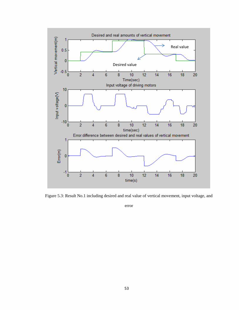
53

Figure 5.3: Result No.1 including desired and real value of vertical movement, input voltage, and

error

Real value

Desired value

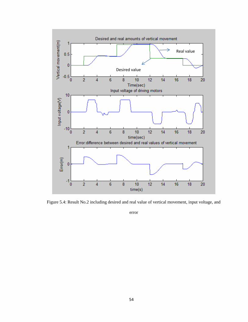
54


error

Real value

Desired value

55


error

Real value

Desired value

56


error

Real value

Desired value

57

Figure 5.7: Result No.5 including desired and real value of vertical movement, input

voltage, and error

5.2.3 Selection of Training Data

The simulation results shown in the previous section were sorted based on user’s

expertise gained over numerous practices. These results were evaluated based on

consistency and how well the reference trajectory was traced.

Real value

Desired value

58

5.2.3.1 Consistency

In this section, the results obtained in section 5.2.2 are evaluated based on consistency. In

this evaluation, calculated correlation coefficient (a statistical measure based on signal

correlation) was used. Each result consists of two increasing steps (named step1 and

step2) and two decreasing steps (named step3 and step4). Consistency between step1 and

2 and between step 3 and 4 was measured. The average of these two values can display

the consistency of the result.

The following sections explain how to calculate the correlation coefficient for the

obtained results:

The correlation coefficient is a concept from statistics to measure how well the trend of a

collection of data fits with another collection. For instance, it can be used to measure how

well a collection of predicted values fits with the real data.

The correlation coefficient is a number between 0 and 1. If there is no similarity between

the collections of data, the value of the correlation coefficient is 0. On the other hand, if

two collections of data have the same trend, the value of the correlation coefficient is

equal to 1.

To define the correlation coefficient, first consider the sum of squared values SSxx,

SSxy, and SSy as below where (xi , yi) is a pair of data, “n” is the number of pair data,

and x , y , and xy are the average amounts of x, y, and xy respectively.

59

SSxx = x2 − nx 2

SSyy = y2 − ny 2

SSxy = xy − nx y

5.3

The correlation coefficient, corr, is then defined by:

𝑐𝑜𝑟𝑟2 =𝑆𝑆𝑥𝑦

2

𝑆𝑆𝑦𝑦 𝑆𝑆𝑥𝑥 5.4

Output voltages versus input errors for five results are shown in Figures 5.8 to 5.12. The

correlation coefficient for increasing steps and decreasing steps is calculated using the

“corrcoef” command in Matlab. The correlation coefficient of the steps is shown in table

5.1.

60

Figure 5.8: Change of voltage in terms of error for four steps of result No.1

61


62


63


64


65

Table 5.1: Correlation coefficient of five different results

Result No.

Correlation

coefficient for

upward steps

Correlation coefficient

for downward steps

Average

correlation

coefficient

1 0.9544 0.6362 0.7953

2 0.9330 0.5688 0.7509

3 0.9547 0.7688 0.86175

4 0.9544 0.7935 0.87395

5 0.9701 0.8848 0.92745

As can be derived from table 5.1, result No.5 has the best consistency.

5.2.3.2 Tracing Reference Trajectory

To evaluate the results in terms of tracing the reference trajectory, the factors of settling

time, rise time and percentage of overshoot are used. Table 5.2 shows the average settling

time with a 3% criterion (Ts), average rise time (Tp) and average percentage of overshoot

for the results shown in section 5.2.2.

66

Table5.2: Average Tp, average Ts, and percentage of overshoot for each result

Average Tp

(sec)

Average Ts

(sec)

(3% criterion)

Percentage of

overshoot

Result 1 2.71 3.29 8.95

Result 2 2.38 2.83 3.39

Result 3 2.21 2.60 4.17

Result 4 2.11 2.72 4.05

Result 5 2.09 2.10 0.77

Result No. 5 shows the best result based on tracing the reference trajectory. This result

has the minimum average rise time, average settling time, and percentage of overshoot.

Referring to table 5.1 and table 5.2, result No.5 is selected from among the five results

discussed in section 5.2.2.

5.2.4 Training Data Preparation

Three following steps were performed to prepare the training data:

Step1, data smoothing: Data received from the Human in the Loop Control Process is in

meters with multiple decimal digits. The precision of the presented robot is defined in

centimetres, therefore inputting numbers with two decimal digits is sufficient. Reducing

the number of decimal digits results in decreased noise in the system. Therefore, input

numbers in ANFIS were rounded to two decimal digits.

Step2, calculating the output data related to equal pair inputs: In the training data

obtained from step1, there are some equal input pairs which have different outputs. When

67

the numbers were rounded in step1 some of the input values became similar while their

related outputs remained different. The data in this form cannot be used to train the

ANFIS. In order to resolve the issue for the sets with similar inputs and different output

the average of the outputs was calculated and used in training the ANFIS. The number of

equal input pairs which have different outputs can be used as a factor to evaluate the

consistency of the data. To count the number of these data pairs, the command of

COUNTIFS can be used in Microsoft Excel. To calculate the average outputs of the

repeated pair inputs, the command of SUMIFS in Microsoft Excel can be used.

Step3, removing repeated data: Step2 causes some repeated pair data with equal inputs

and output. To remove this repeated pair data the command REMOVE DUPLICATE is

used. After removal of the duplicate pairs whose inputs are repeated, the remaining pairs

are fed into the ANFIS for tuning.

Table 5.3 gives an example of the above steps. This table consists of 4 columns. In first

column, there are 7 pairs of data before improvement. In the next column the amounts in

the first column are rounded. In the third column the average of the outputs whose related

inputs are equal is calculated and the repeated pair data is removed.

68

Table 5.3: An example of improving pair data

Before preparation

After step1

(round)

After step2

(average)

After step3

(remove)

Input1 Input2 Output Input1 Input2 Output Input1 Input2 Output Input1 Input2 Output

0.3146 0.3146 3.2012 0.31 0.31 3.20 0.31 0.31 3.31 0.31 0.31 3.31

0.3123 0.3146 3.4232 0.31 0.31 3.42 0.31 0.31 3.31 0.47 0.31 3.64

0.4683 0.3123 3.6446 0.47 0.31 3.64 0.47 0.31 3.64 0.47 0.47 4.32

0.4665 0.4683 4.2014 0.47 0.47 4.20 0.47 0.47 4.32 0.52 0.47 4.62

0.4712 0.4665 4.4364 0.47 0.47 4.44 0.47 0.47 4.32 0.53 0.52 4.84

0.5214 0.4712 4.6181 0.52 0.47 4.62 0.52 0.47 4.62 - - -

0.5334 0.5214 4.8398 0.53 0.52 4.84 0.53 0.52 4.84 - - -

From 2000 pair data points obtained from the best human-in the-loop control process

from section 5.2.3, 200 pairs remained after improvement. Figure 5.13 and figure 5.14

deal with the final voltage and error amounts which are used to train the ANFIS

respectively.

69

Figure 5.13: Filtered voltage used to tune the ANFIS

Figure 5.14: Filtered error amount used to tune the ANFIS

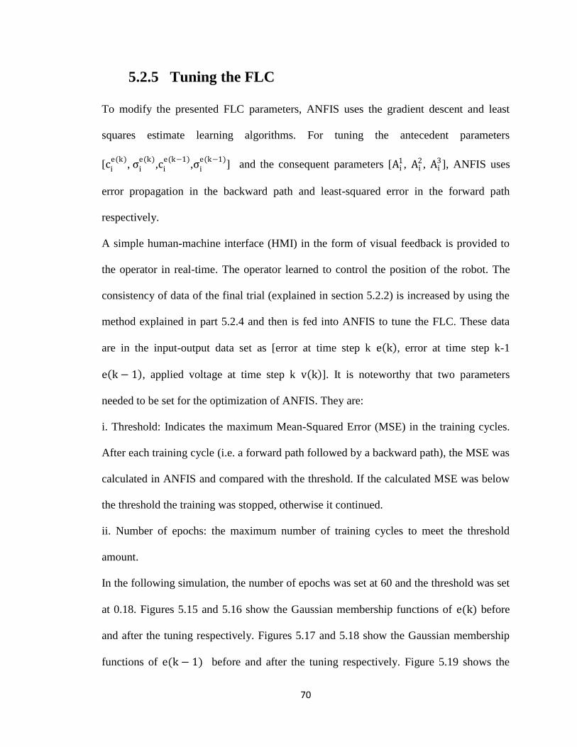
70

5.2.5 Tuning the FLC

To modify the presented FLC parameters, ANFIS uses the gradient descent and least

squares estimate learning algorithms. For tuning the antecedent parameters

[cie(k)

, σie(k)

,cie(k−1)

,σie(k−1)

] and the consequent parameters [Ai1, Ai

2, Ai3], ANFIS uses

error propagation in the backward path and least-squared error in the forward path

respectively.

A simple human-machine interface (HMI) in the form of visual feedback is provided to

the operator in real-time. The operator learned to control the position of the robot. The

consistency of data of the final trial (explained in section 5.2.2) is increased by using the

method explained in part 5.2.4 and then is fed into ANFIS to tune the FLC. These data

are in the input-output data set as [error at time step k e k , error at time step k-1

e k − 1 , applied voltage at time step k v k ]. It is noteworthy that two parameters

needed to be set for the optimization of ANFIS. They are:

i. Threshold: Indicates the maximum Mean-Squared Error (MSE) in the training cycles.

After each training cycle (i.e. a forward path followed by a backward path), the MSE was

calculated in ANFIS and compared with the threshold. If the calculated MSE was below

the threshold the training was stopped, otherwise it continued.

ii. Number of epochs: the maximum number of training cycles to meet the threshold

amount.

In the following simulation, the number of epochs was set at 60 and the threshold was set

at 0.18. Figures 5.15 and 5.16 show the Gaussian membership functions of e(k) before

and after the tuning respectively. Figures 5.17 and 5.18 show the Gaussian membership

functions of e(k − 1) before and after the tuning respectively. Figure 5.19 shows the

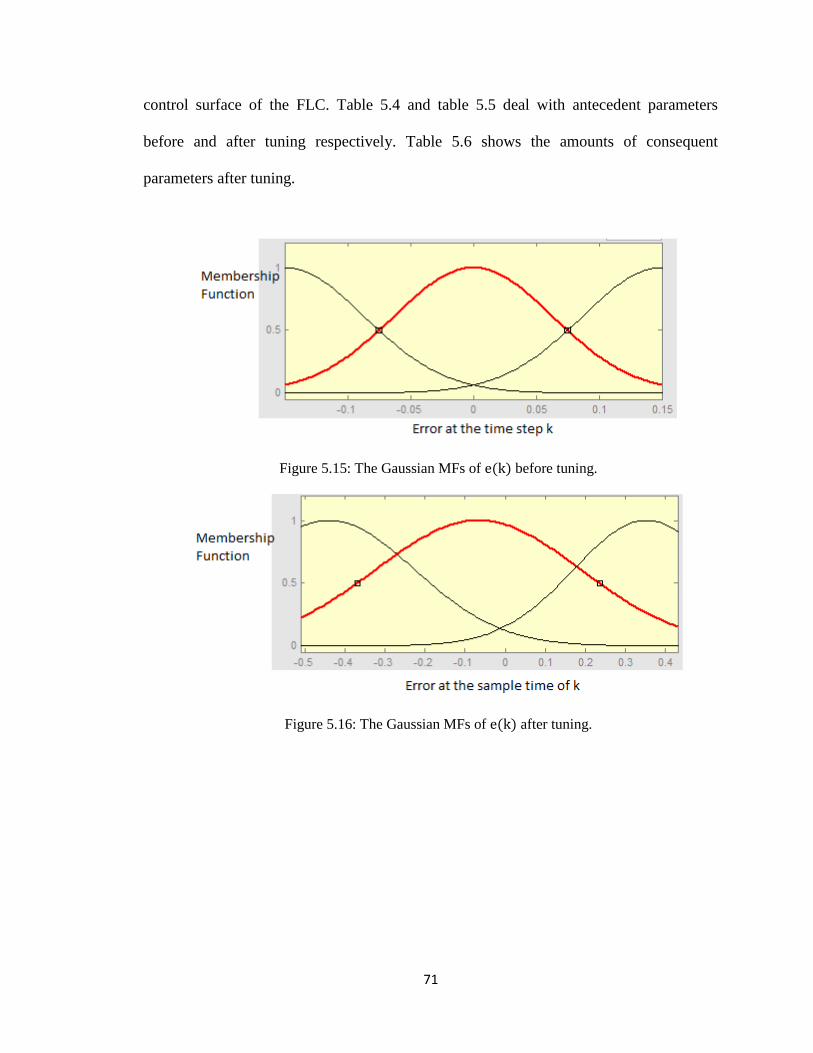
71

control surface of the FLC. Table 5.4 and table 5.5 deal with antecedent parameters

before and after tuning respectively. Table 5.6 shows the amounts of consequent

parameters after tuning.

Figure 5.15: The Gaussian MFs of e(k) before tuning.

Figure 5.16: The Gaussian MFs of e(k) after tuning.

72

Figure 5.17: The Gaussian MFs of e(k − 1) before tuning.

Figure 5.18: The Gaussian MFs of e(k − 1) after tuning.

Figure 5.19: The control surface.

73

Table 5.4: Antecedent parameters before tuning

Rule No. 𝐜𝐢𝐞(𝐤)

𝛔𝐢𝐞(𝐤)

𝐜𝐢𝐞(𝐤−𝟏)

𝛔𝐢𝐞(𝐤−𝟏)

1 0.0637 -0.15 0.2017 -0.52

2 0.0637 -0.15 0.2017 -0.045

3 0.0637 -0.15 0.2017 0.43

4 0.0637 0 0.2017 -0.52

5 0.0637 0 0.2017 -0.045

6 0.0637 0 0.2017 0.43

7 0.0637 0.15 0.2017 -0.52

8 0.0637 0.15 0.2017 -0.045

9 0.0637 0.15 0.2017 0.43

74

Table 5.5: Antecedent parameters after tuning

Rule No. 𝐜𝐢𝐞 𝛔𝐢

𝐞 𝐜𝐢𝐞 𝛔𝐢

𝐞

1 0.2141 -0.4393 0.1596 -0.354

2 0.2141 -0.4393 0.3415 -0.089

3 0.2141 -0.4393 0.0549 0.1342

4 0.2565 -0.0672 0.1596 -0.354

5 0.2565 -0.0672 0.3415 -0.089

6 0.2565 -0.0672 0.0549 0.1342

7 0.1822 0.3519 0.1596 -0.354

8 0.1822 0.3519 0.3415 -0.089

9 0.1822 0.3519 0.0549 0.1342

75

Table 5.6: Consequent parameters after tuning

Rule No. 𝐀𝐢𝟏 𝐀𝐢

𝟐 𝐀𝐢𝟑

1 -5.799 10.22 -15.01

2 9.979 38.24 30.66

3 -83.77 -122.4 420.5

4 -20.47 -21.68 -12.95

5 103.6 -49.15 -0.828

6 -38.51 -23.73 -45.77

7 -10.22 -4.734 -75.83

8 5.944 16.28 -4.831

9 -365.8 44.08 115.7

76

5.2.6 Simulation Result

The ANFIS, tuned as explained in previous sections, is used as a controller in a closed-

loop as shown in Figure 5.20.

Figure 5.20: Implementation of an ANFIS controller in the closed-loop

Figure 5.21 deals with tracing a reference trajectory which is different from the trajectory

used for collecting training data. Figure 5.22 shows the response of the ANFIS controller.

Figure 5.21: Tracing the reference trajectory using ANFIS

Time step (0.01 Sec)

Real value

Desired value

77

Figure 5.22: Response of the ANFIS controller

5.2.7 Real-time Experiments

The robot was tested on a pole. The pole was a 2.5-meter long 2-inch PVC pipe mounted

on a stable platform. A Logitech Attack 3 Joystick was used for controlling the robot’s

motion in a human-in the-loop control process. Lynxmotion quadrature incremental

optical encoders were also used as interoceptive sensors to measure the vertical position

of the robot. Optical encoders were calibrated offline. The operator interfaces to the

robot via a computer using Simulink, real-time workshop toolbox, and Wincon [47].

Figure 5.23 shows a snapshot of the physical apparatus. The hardware used in the

experiments include: Two Advanced voltage-controlled linear servo amplifiers along


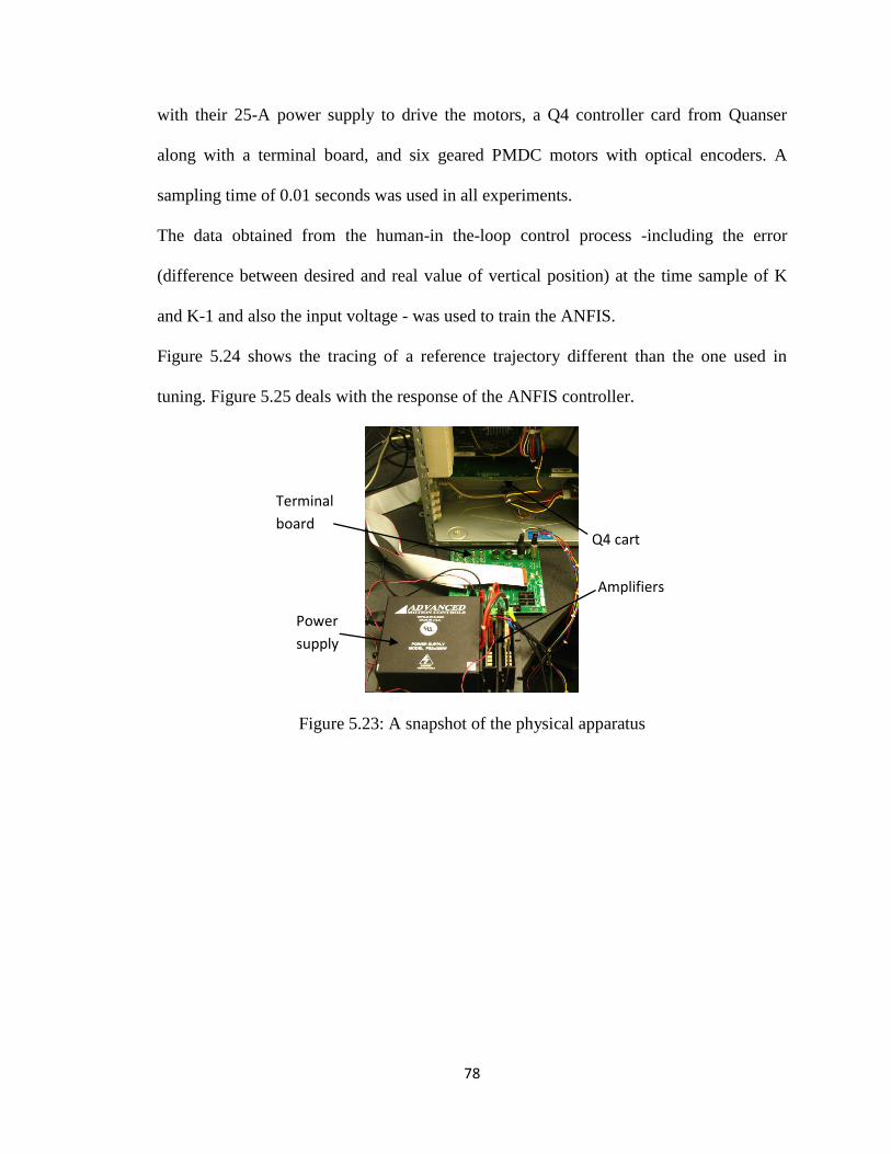
78

with their 25-A power supply to drive the motors, a Q4 controller card from Quanser

along with a terminal board, and six geared PMDC motors with optical encoders. A

sampling time of 0.01 seconds was used in all experiments.

The data obtained from the human-in the-loop control process -including the error

(difference between desired and real value of vertical position) at the time sample of K

and K-1 and also the input voltage - was used to train the ANFIS.

Figure 5.24 shows the tracing of a reference trajectory different than the one used in

tuning. Figure 5.25 deals with the response of the ANFIS controller.

Figure 5.23: A snapshot of the physical apparatus

Power

supply

Amplifiers

Q4 cart

Terminal

board

79

Figure 5.24: Tracing the reference trajectory using an ANFIS controller in an

experimental test

Figure 5.25: Response of an ANFIS controller in an experimental test



Real value

Desired value

80

5.3 PID Controller

In this section a Proportional Integral Derivative (PID) controller is used to control the

vertical position of the robot. A classical PID controller is in the form of:

u t = kp e t + kd

de

dt+ kI e τ dτ

t

0

5.5

Where u is output of the controller, e is error (difference between actual and desired

values of the controlled variable), kp is proportional gain, kd is derivative gain, and kI is

integral gain.

In designing a PID controller the following specifications should be considered [48]:

Stability robustness;

Set-point following and tracking performance at transient, including rise-time, overshoot

and settling time;

Regulation performance at steady-state, including load disturbance rejection;

Robustness against system modeling uncertainty;

Noise attenuation and robustness against environmental uncertainty.

The presented PID controller is tuned with the Ziegler-Nichols method [49] and the best

values for proportional, derivative and integral gains are kp=500, kd=150, and kI=10

respectively.

The functionalities of each term in equation 5.25 are as follows [48]:

1) The proportional term provides an overall control action proportional to the error

signal through the all-pass gain factor.

2) The derivative term improves transient response through high-frequency

compensation by a differentiator.

81

3) The integral term reduces steady-state errors

The individual effects of the above terms on the control performance are summarized in

Table 5.7

Table 5.7: Effect of independent P and D tuning [48]

Closed-

Loop

Response

Rise time Overshoot

Settling

time

Steady-

State

Error

Stability

Increasing

𝐤𝐩 Decrease Increase

Small

increase

Decrease Degrade

Increasing

𝐤𝐝

Small

decrease

Decrease Decrease

Minor

change

Improve

Increasing

𝐤𝑰

Small

decrease

Increase Increase

Large

Decrease

Degrade

Figure 5.26 shows the tracing of a reference trajectory using a PID controller. Figure 5.27

deals with response of the PID controller

82

Figure 5.26: Tracing a reference trajectory using a PID controller


Real value

Desired value

83

Figure 5.27: Response of the PID controller

5.4 Discussion

5.4.1 FLC vs. PID Controller

As can be seen in the previous sections, the ANFIS controller tuned by data captured

from the human-in-the-loop control process is not only able to control the vertical

movement of the robot, but also possess the following advantages in comparison to the

PID controller.

1. Response time: the average settling time for the system controlled by the ANFIS

controller is 2.13 while this time for the PID controller is 2.35. This shows that by using


84

an ANFIS controller instead of a PID controller, we can decrease the settling time by as

much as 9.36%.

2. Actuator Saturation: The maximum control signal while using the ANFIS controller is

4.82 volts, while the PID controller reached a maximum of 7.2 volts. This shows that the

ANFIS requires 33% less voltage.

3. Energy expenditure: Since the average voltage provided to the motors reflects the total

energy expenditure of the system, one can observe that when using a PID controller the

average voltage expenditure of the system is 4.81 volt while this amount in case of using

a FLC is 3.92 volt which demonstrates an 18.52% reduction.

5.4.2 Effects of Improving Training Data

As mentioned in section 5.2.4, to improve the training data three steps have been done:

data smoothing, calculating the output data related to equal pair inputs, and removing

duplicated data. Figure 5.28 shows the tracing reference trajectory in condition of using

an ANFIS controller which is tuned with pair data before removing repeated data.

As can be derived from figures 5.28 and 5.21, removing repeated pair data produces a

lower error in tracing results.

85

Figure 5.28: Tracing the reference trajectory using the ANFIS controller which is tuned with all pair data


Real value

Desired value

86

Chapter 6

Conclusion and Future Work

6.1 Conclusion

The work presented in this thesis includes two main areas as follows:

1) Design and development of a new re-configurable wheeled climbing robot. This robot

benefits from a novel design with high simplicity and versatility simultaneously. This

robot is capable of doing a multitude of tasks that no other single robot could do in

the past. Some of these tasks are climbing staircases, moving inside empty ducts

and/or pipes, climbing over ropes/poles with varying cross sections, shapes, and

sizes, jumping over obstacles with proper motion coordination and moving inside

narrow passageways. The design of this robot allows it to traverse a wide range of

unconventional terrains and makes it a novel concept.

87

2) Design and implementation of a stand-alone fuzzy logic controller (FLC) for control

of vertical movement of the mentioned robot. For tuning the parameters of the fuzzy

logic controller a new method is used to reach the best results approximating the

human operator actions. In this method (unlike previous research in the area of fuzzy

logic control) the numerical information gained from the optical encoders in the

human-in the-loop control process is directly utilized to tune the controller

parameters in an adaptive neuro-fuzzy inference system (ANFIS). In this regard,

Major contributions can be categorized as follows:

Avoiding the tedious task of mathematical modeling of the system.

Avoiding the tedious task of deriving linguistic rules.

Achieving superior performance in terms of rise/settling time, overall energy

expenditure and actuator saturation than a mechanistic controller (PID

controllers).

6.2 Future Work

The future work is threefold:

1) In this thesis, a new re-configurable wheeled climbing robot was introduced.

Although this robot can be categorized as a novel and versatile climbing robot, we

focused on straight pole climbing among all application domains. The dynamics

of the robot can be analyzed in other application domains as outlined below:

Curved pole climbing:

Rope climbing

Stair climbing

88

Duct climbing

Duct climbing with varying cross section

Rough-terrain rover

Pipe-crawling robot

Moving through difficult passageways

Carrying a payload

2) Using an external sensor to measure the vertical movement. This amount can be

compared with what is measured with the encoders. If the vertical movement

measured from the external sensor is greater than the vertical movement measured

from encoders, one can conclude that slippage happens. In this condition the angle

between arms should be increase to create more normal force and thus friction

force.

89

Bibliography

[1] F. Xu, X. Wang. A wheel-Based Cable Climbing Robot with Descending Speed

Restriction. In Proc. CCDC Control and Decision Conference, pages 1570-1575, July

2008.

[2] Q. Quan,S. Ma. A modular crawler-driven robot: Mechanical design and preliminary

experiments. In Proc. IEEE/RSJ International Conference on Intelligent Robots and

Systems, pages 639-644, Oct 2009.

[3] R.T.M’closkey, J.W.Burdick, A.F.Vakakis. On the periodic motions of simple

hopping robots. In Proc. IEEE International Conference on Systems, Man and

Cybernetics, pages 771-777, Nov1990.

[4] E. Foo, Thanh Tung Le. STARCLY robot-A novel compact stair climbing robot. In

Proc. of 2nd ICMEE International Conference, vol. 2, pages. 75-78, Aug 1990.

[5] N.D.Hewapathirana, L. Uddawatta, J.P. Karunadasa, T.Nanayakkara. Analysis on

four legged multipurpose rope climbing robot. In Proc. of the ICIIS International

Conference on Industrial and Information systems, pages 505-510, Dec 2009.

90

[6] W. Yan, L. Shuliang, X. Dianguo etc. Development and application of wall-Climbing

Robots. In Proc. of IEEE International Conference on Robotics and Automation, vol. 2,

pages 1207-1212, May 1999.

[7] L.Briones, P. Bustamante, M. A. Serna. Wall-climbing robot for inspection in nuclear

power plants. In Proc. of IEEE International Conference on Robotics and Automation,

Vol. 2, pages 1409-1414, May1994.

[8] G.La Rosa, M.Messina, G.Muscato. A low-cost lightweight climbing robot for the

inspection of vertical surfaces. In Mechatronics, Vol. 12, Issue1, pages 71-96, Feb. 2002.

[9] M.S. Wang, Y.M. Tu. Design and implementation of a stair-climbing robot. In Proc.

IEEE workshop on Advanced robotics and Its Social Impacts, pages 1-6, Aug 2008.

[10] S. Kim, M. Spenko, S. Trujillo, B. Heyneman, D. Santos, and M. Cutkosky. Smooth

vertical surface climbing with directional adhesion. In Proc. of IEEE Transactions on

Robotics, vol. 24, no. 1, pages 65 –74, Feb 2008.

[11] M.Krishna, J.Bares, E.Mutschler. Tethering system design for Dante II. In Proc. of

IEEE, International Conference on Robotic and Automation, vol. 2, pages 1100-1105,

Apr 1997.

[12] B.Yazdani, M. Nili ahmadabadi, A. Harati, H.Moaveni and N.Solati. Design and

development of a pole climbing robot mechanism. In the proceedings of mechatronics

and robotics, Germany, Sep.2004.

91

[13] G. Vastianos. SLOTH Rope Climbing Robot. In Electronics Department, Faculty of

Technological Applications, Technological Educational Institute of Piraeus, Greece,

2002.

[14] T.Okada, T. Kanade. Three-Wheeled self-Adjusting vehicle in pipe. Int. J. of

Robotics Research. Vol.6 No.4, pages 60-75, winter 1987.

[15] G.H.Eckert, D.Gebrath, H.Schlusen. In-pipe Inspection and repair Equipment. In

Annual Meeting of American Nuclear Society, Reno, Nevada, June 15-19, 1986.

[16] A.Madhani, S.Dubowsky. Motion Planing of Mobile Multi-limb Robotic Systems

Subject to Force and Friction Constrains. In Proc. IEEE Robotics and Automation, pages

133-139, Nice, France, May 1992.

[17] W. Neubauer. A Spider-like Robot that Climbs Vertically in Ducts or Pipes. In Proc.

IEEE/RSJ/GI International Conference, Vol. 2, pages 1178-1185, Sep1994.

[18] C. Ratanasawanya, P. Binsirawanich, M. Yazdanjo, M. Mehrandezh, S. Poozesh, R.

Paranjape, and H. Najjaran. Design and Development of a Hardware-in-the Loop

Simulation System for a Submersible Pipe Inspecting Robot. In Electrical and Computer

Engineering, 2006. CCECE’06. Canadian Conference on, pages 1526–1529, 2006.

[19] KJ Astrom, T.J. McAvoy, Intelligent control: an overview and evaluation. Handbook

of Intelligent Control, D. White and D. Sofge, eds., VNR Computer Library, Van-

Nostrand Reinhold, New York, NY, 1992.

[20] PJ Antsaklis. Intelligent learning control. IEEE Control Systems Magazine, 15(3):5–

7, 1995

92

[21] H.W.Beaty. Handbook of electric power calculations. New York: Mcgraw-Hill,

2000.

[22] LA Zadeh. Fuzzy sets. World Scientific Publishing Co., Inc. River Edge, NJ, USA,

1996.

[23] LA Zadeh. Outline of a new approach to the analysis of complex systems and

decision processes. In IEEE Transactions on Systems, Man, and Cybernetics, Vol. SMC-

3, pages 28–44, 1973.

[24] EH Mamdani et al. Application of fuzzy algorithms for control of simple dynamic

Plant. In Proc. Iee, Vol. 121, Issue 12, pages 1585–1588, 1974.

[25] S.Ahn, Y. Ho, K. Wook, H. Kwon. Design of a fuzzy logic controller module for a

loop controller. In Proc. IEEE International Conference on Industrial Technology, pages

598-602, 1996.

[26] S Mishra. TS-fuzzy controlled active power filter for load compensation. In IEEE

Power Engineering Society General Meeting, 2006.

[27] A.F. Amer, E.A. Sallam, W.M. Elawady. Fuzzy pre-compensated fuzzy self-tuning

fuzzy PID controller of 3 DOF planar robot manipulators. In IEEE/ASME International

conference on Advanced intelligent mechatronics, pages 599-604, July 2010.

[28] Q.Li, D.Shen. A New Incremental Fuzzy PD + Fuzzy ID Fuzzy Controller. In WASE

International Conference on Information Engineering, Vol. 1, pages 615-619, 2009.

[29] W.Qi, Z.Lingzhi, Z.Shuangxi. A novel fuzzy logic secondary voltage controller. In

International conference of Power System Technology, Vol.4, pages 2589-2593, Dec.

2002.

http://ieeexplore.ieee.org/xpl/mostRecentIssue.jsp?punumber=11204

93

[30] W.Pedrycz, Z.A.Sosnowski. Genetically optimized fuzzy decision trees. In IEEE

Transaction on Systems, Man, Cybernetics, Vol.35, pages 633-641, 2005.

[31] JM Keller, Y. Hayashi, Z. Chen. Interpretation of nodes in networks for fuzzy logic.

In Second IEEE International Conference on Fuzzy Systems, pages 1203–1207, 1993.

[32] D.Chen, J.Yang, B.Xu. Adaptive optimal control of a class of uncertain nonlinear

systems using fuzzy logic and neural networks. In IEEE Conference on Decision and

Control, Vol.5, pages 5094-5099, 2005.

[33] A.M.Sharof, T.T. Lie. A robust artificial neural network based speed/voltage

regulator for synchronous generators. In Proc. IEEE International Symposium on

Industrial Electronics, Vol.1, pages 384-389, 1995.

[34] J. Yao, L.Wang, C.Wang, Z.Zhang, P.Jia. ANN-based pid controller for an electro-

hydraulic servo system. In International Conference on Automation and Logistics, pages

18-22, 2008.

[35] M.R.Sindhu, M.G.Nair, T.N.P. Nambiar. An ANN based Digital Controller for a

Three-phase Active Power Filter. In International Conference on Power System

Technology and IEEE Power India Conference, pages 1-7, 2008.

[36] P.K.Singh, P.Rai. An ANN based X-PC target controller for speed control of

permanent magnet brushless DC motor. In IEEE Conference on Control Application,

pages 1027-1032, 2005.

[37] V.Chandrasekar, L.Hongping. An adaptive neural network scheme for precipitation

estimation from radar observations. In Proc. IEEE International, Geoscience and Remote

Sending Symposium, Vol.4, pages 1895-1897, 2002.

http://ieeexplore.ieee.org/xpl/mostRecentIssue.jsp?punumber=3587

http://ieeexplore.ieee.org.libproxy.uregina.ca:2048/search/searchresult.jsp?searchWithin=Authors:.QT.Sindhu,%20M.R..QT.&newsearch=partialPref

http://ieeexplore.ieee.org.libproxy.uregina.ca:2048/search/searchresult.jsp?searchWithin=Authors:.QT.%20Nair,%20M.G..QT.&newsearch=partialPref

http://ieeexplore.ieee.org.libproxy.uregina.ca:2048/search/searchresult.jsp?searchWithin=Authors:.QT.%20Nambiar,%20T.N.P..QT.&newsearch=partialPref

94

[38] S.Xu, M.Zhang. Data mining - an adaptive neural network model for financial

analysis. In Third International Conference on Information Technology and Applications,

Vol.1, pages 336-340, 2005.

[39] M.J.Ismail, R.Ibrahim, I.Ismail. Adaptive neural network prediction model for

energy consumption. In International Conference on Computer Research and

Development, Vol.4, pages 109-113, 2011.

[40] Y.Guo, L.Chen. Adaptive neural network control of coordinated motion of dual-arm

space robot system with uncertain parameters. In Word Conference on Intelligent Control

and Automation, pages 4842-4846, 2008.

[41] C.H.Cai, D.Du, Z.Y.Liu. Battery state-of-charge (SOC) estimation using adaptive

neuro-fuzzy inference system (ANFIS). In International Conference on Fuzzy Systems,

Vol.2, pages 1068-1073, 2003.

[42] C.Venugopal. ANFIS based Field Oriented Control for Matrix Converter fed

Induction Motor. In IEEE International Conference on Power and Energy, pages 74-78,

2011.

[43] M.Buragohain, C.Mahanta. ANFIS Modelling of Nonlinear System Based on

Subtractive Clustering and Combined FFD-Vfold Technique. In Annual IEEE India

Conference, pages 1-6, 2007.

[44] M.Liu, M.Dong, C.Wu. A New ANFIS for Parameter Prediction with Numeric and

Categorical Inputs. In IEEE Transactions on Automation Science and Engineering, Vol.7,

pages 645-653, 2010.

95

[45] P.J.E.Ambrosio, X.Liu, N.A.J.Lieven, J.M.R.Cortes. ANFIS-2D wavelet transforms

approach to structural damage identification. In Annual Meeting of North American Fuzzy

Information Processing Society, pages 1-6, 2011.

[46] D.W.Chen, J.P.Zhang. Time series prediction based on ensemble ANFIS. In Proc.

Of International Conference on Machine Learning and Cybernetics, Vol.6, pages 3552-

3556, 2005.

[47] Quanser Company. http://www.quanser.com, Last visited Aug 2011.

[48] K.H. Ang, G. Chong, Y. Li, Y.E.A.P. Ltd, and S. Singapore. PID control

system analysis, design, and technology. IEEE transactions on control systems

technology, Vol. 13, pages 559–576, 2005.

[49] JG Ziegler, NB Nichols. Optimum settings for automatic controllers. In Journal of

dynamic systems, measurement, and control, pages 115-220, 1993.

[50] F. Jay. IEEE standard dictionary of electrical and electronic terms. Institute of

Electrical & Electronics Engineers, 1977.

[51] J.R.Jang, C.T.Sun, E. Mizutani. Neuro-Fuzzy and Soft Computing: a computational

approach to learning and machine intelligence. 1997.

[52] A.H. Heidari. Human analogous control: analysis, design, and implement. Industrial

System Engineering, University of Regina, 2009.

http://www.quanser.com/

96

Appendix A:

Simulink Model of the Climbing Robot

The dynamic of the robot can be modeled by using Simulink as shown schematically in

figure A.1. In the Simulink model shown in this figure, the embedded functions 1 and 2

were based on equations 4.12 and the embedded functions 2 and 4 were created based on

a combination of equations 4.7 and 4.8. Embedded function 5 was created based on

equation 4.12. Table 4.2 deals with the constant values are used to the Simulink model.

Definition of these constants are cited in table 4.1

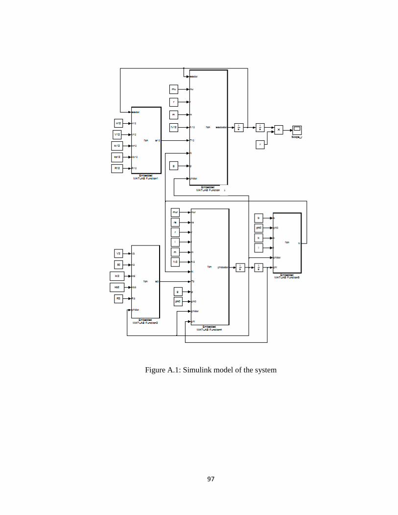
97

Figure A.1: Simulink model of the system

3

98

Appendix B:

Case study: Controlling the Rotation Angle of a DC motor

In this chapter the angular rotation of a DC motor was controlled in two ways: by using a

PD controller and by using an Adaptive Neural Fuzzy Inference System (ANFIS) which

was trained with the dataset obtained from a human-in-the-loop control system. In this

method, an operator tries to track a reference trajectory based on visually-provided

sensory feedback through a Human Machine Interface (HMI) unit. The ANFIS acts as a

controller in a closed loop and its task is to provide proper inputs to the system (in this

case study a geared DC motor) to obtain the desired output which is a specified rotation

angle. In this case study the desired rotation angle is 500 Radians.

B.1 Dynamic Equations

The dynamic of a DC motor can be explained by the formula:

99

θ =kt ∗ V − kb ∗ θ

R ∗ J B.1

Where θ is the rotating angle, V is voltage, R is resistance, J is the rotor inertia, kt is the

torque constant, kb is the Back-EMF constant.

Based on equation B.1, the dynamics of the DC motor can be modeled using Simulink as

shown in figure B.1.

Figure B.1: Simulink model of a DC motor

The value of parameters used in this case study are listed in Table B.1.

100

Table B.1: Parameters of the DC motor used in the case study presented in appendix B

Parameter Value Unit

Torque constant 0.0232 N.m/A

Back-EMF constant 0.0232 V/rad/s

Resistance 1.26 Ohm

Rotor inertia 4.2E-06 Kg.m2

B.2 Conventional Controller

Figure B.2 shows the implementation of the PID controller in a Closed-Loop.

Figure B.2: Implementation of a PID controller in the closed-loop for controlling the

rotation angle of a DC motor

The PID controller was designed in accordance with the Ziegler-Nichols tuning criteria.

The best gain values were found to be Kp = 0.012, Kd = 0.01 and Ki= 0.0001 for the

proportional, derivative, and integral gains respectively.

Figure B.3 and B.4 show the response of the PID controller (output voltage) and the tracing

of the reference trajectory respectively.

101

Figure B.3: Output of the PID controller to control the rotation angle of a DC motor

102

Figure B.4: Rotation angle of a DC motor using a PID controller

B.3 Unconventional Controller

In this part, an ANFIS controller is used as an unconventional controller. ANFIS is a

fuzzy logic system whose membership functions and rules parameters can be tuned to

benefit from learning. To tune these parameters, ANFIS uses a multilayer neural network.

Each layer consists of some nodes and each node performs a function so that the entire

network is equivalent to a fuzzy system. An operator tries to track a reference trajectory

based on visually-provided sensory feedback through a Human Machine Interface (HMI)

unit and the data gained in this process is used to train the ANFIS. The trained ANFIS

was used as a controller to trace a reference trajectory different than that used for

training.

Real value

Desired value

103

Structure of the FLC

The fuzzy system used in the presented ANFIS is a first-order TSK type. The inputs of

the ANFIS are error in the rotation angle of the DC motor and the rate of change in the

error as follows:

e t = r − θ(t)

e t = −θ (t) B.3

Where ”r” is the reference trajectory.

Three membership functions (MF) are chosen for each input. The MFs are Gaussian type

in the form of:

𝑓 𝑥; 𝑐, 𝜎 = 𝑒− 𝑥−𝑐 2

2𝜎2 B.4

The FLC consists of 9 rules in the general form of:

𝑢𝑖 = 𝐴𝑖1𝑒𝑖 + 𝐴𝑖

2𝑒 𝑖 + 𝐴𝑖3 B.5

Where, “i” denotes the number of the rule.

The control signal (output of the FLC) was the weighted average of the nine rule-outputs.

The response of the FLC is affected by the value of the antecedent parameters

[cie , σi

e ,cie ,σi

e ] and consequent parameters [Ai1, Ai

2, Ai3] of each rule “i”. To gain the best

results, similar to those obtained by a human operator, the above parameters are tuned

using the ANFIS. Figures B.5 and 5.6 show the membership functions of input 1 (error)

before and after the tuning respectively. Figure B.7 and figure B.8 show the membership

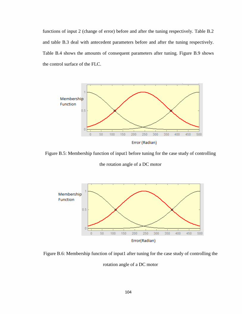
104

functions of input 2 (change of error) before and after the tuning respectively. Table B.2

and table B.3 deal with antecedent parameters before and after the tuning respectively.

Table B.4 shows the amounts of consequent parameters after tuning. Figure B.9 shows

the control surface of the FLC.

Figure B.5: Membership function of input1 before tuning for the case study of controlling

the rotation angle of a DC motor

Figure B.6: Membership function of input1 after tuning for the case study of controlling the


105

Figure B.7: Membership function of input2 before tuning for the case study of controlling

the rotation angle of a DC motor

Figure B.8: Membership function of input2 after tuning for the case study of controlling the


106

Figure B.9: Control surface of the FLC for the case study of controlling then rotation angle

of a DC motor

107

Table B.2: Antecedent parameters before tuning for the case study of controlling the rotation

angle of a DC motor



𝐞

1 109.7 -16.42 25.21 -111.3

2 109.7 -16.42 25.21 -51.92

3 109.7 -16.42 25.21 7.441

4 109.7 241.8 25.21 -111.3

5 109.7 241.8 25.21 -51.92

6 109.7 241.8 25.21 7.441

7 109.7 500 25.21 -111.3

8 109.7 500 25.21 -51.92

9 109.7 500 25.21 7.441

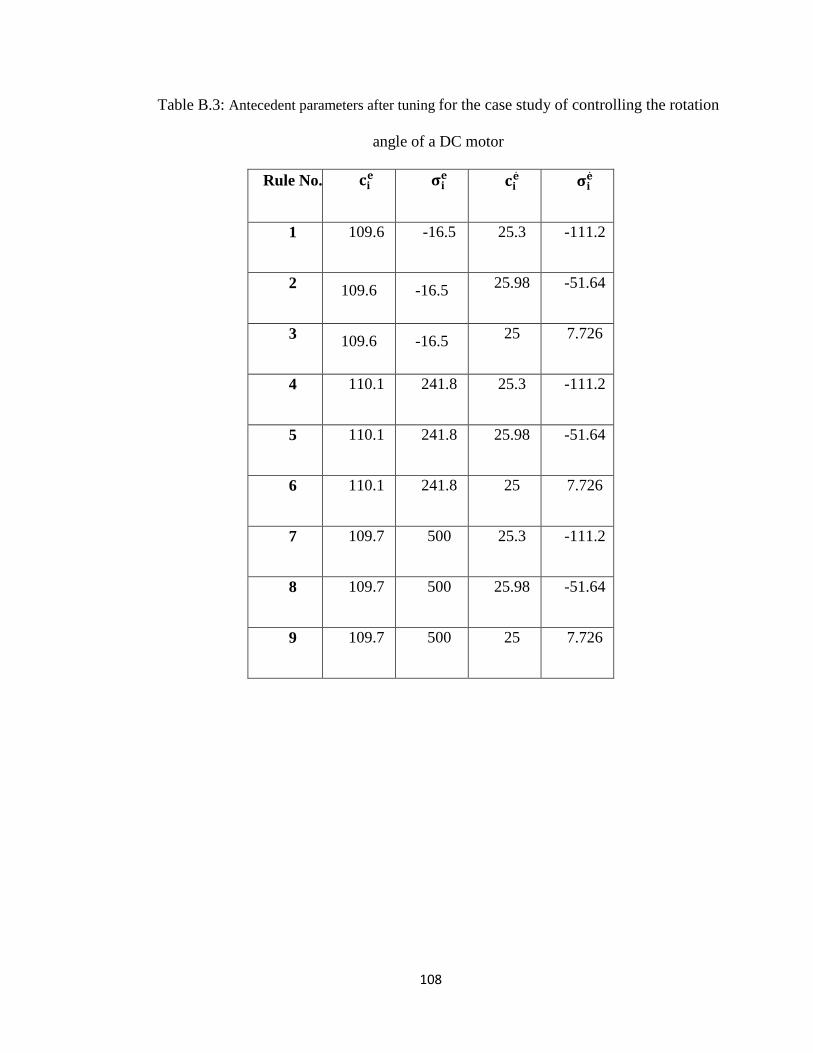
108

Table B.3: Antecedent parameters after tuning for the case study of controlling the rotation

angle of a DC motor



𝐞

1 109.6 -16.5 25.3 -111.2

2 109.6 -16.5

25.98 -51.64

3 109.6 -16.5

25 7.726

4 110.1 241.8 25.3 -111.2

5 110.1 241.8 25.98 -51.64

6 110.1 241.8 25 7.726

7 109.7 500 25.3 -111.2

8 109.7 500 25.98 -51.64

9 109.7 500 25 7.726

109

Table B.4: Consequent parameters after tuning for the case study of controlling the rotation

angle of a DC motor

Rule No. 𝐀𝐢𝟏 𝐀𝐢

𝟐 𝐀𝐢𝟑

1 -0.096 0.1214 21.32

2 1.278 1.821 47.71

3 -2.659 -2.408 -202.1

4 -0.088 -0.1186 17.26

5 1.279 9.387 748.6

6 -14.62 48.59 2038

7 0.0393 0.7827 -42.08

8 0.8471 1.145 -405.5

9 2.275 -3.294 -816.1

Figure B.10 and B.11 show the response of the fuzzy logic controller (output voltage) and

the tracing of the reference trajectory respectively.

110

Figure B.10: Response of the fuzzy logic controller for the case study of controlling the


Figure B.11: Rotation angle of a DC motor using a fuzzy logic controller for the case

study of controlling the rotation angle of a DC motor

111

B.4 Comparing Conventional and Unconventional Controllers

As can be seen in figure B.11, the FLC tuned by human data can trace the reference

trajectory of r=500 radian. Based on the result shown in figures B.5, B.6, B.10, and B.11,

one can conclude that the FLC has three advantages over the PID controller:

1. Faster response: the settling time for the system controlled by the FLC is 10.43 while

this time for the PID controller is 12.28.

2. Less overshoot: The amount of overshoot for the system controlled by the PID

controller was 508 radians, which is a 1.6% overshoot. Using the FLC reduced this

amount to near zero.

3. Actuator Saturation: The maximum control signal using the FLC is 4.75 volts while

that of the PID controller is 6 volts. This shows that the FLC demonstrates a 26.3%

reduction in max voltage used.

112

Appendix C

Basic Definitions Used in This Thesis

This section contains some definitions used in control, fuzzy logic controllers and

ANFIS.

System:

A system is a combination of components that act together to perform a function which

cannot be achieved by any of those components individually [50].

Servomechanism:

Servomechanism is a mechanism to control the mechanical position or velocity of a

system by using error feedback. For example the cruise control of a car is a

servomechanism.

Human Analogous Control:

113

Human analogous control is a control process in which human behaviour is emulated.

Neural networks and fuzzy logic systems are the most well-known areas for developing

human analogous controls.

Neural networks:

A neural network is a network structure which is composed of a number of nodes

connected by some links [51]. Each node is a process unit and each link represents the

relationship between nodes. In an adaptive neural network, the nodes are adaptive. This

means that the output of all or part of the nodes depends on some modifiable parameters

of the node. These parameters are tuned in such a way that the difference between the

output of the network and the expected output is minimal.

In the most cases, each node of the adaptive network has its own function and each link is

used to specify the propagation direction of node outputs while no weights or parameters

are associated with links. Figure 5.1 shows a typical adaptive network with two outputs

and two inputs.

114

Figure C.1: A Feedforward Adaptive Network

Each node possesses local parameters which are a part of the network parameters. In

other words, the union of all node parameters is the network’s overall parameter set. One

can divide the nodes of a network into two main parts: adaptive nodes and fixed nodes. If

a node’s parameter set is not empty, that node is adaptive. The function of an adaptive

node depends on the parameter values. On the contrary, if a fixed node has an empty

parameter set, then its function does not depend on parameter values and is fixed. Usually

adaptive and fixed nodes are represented by squares and circles respectively (see figure

C.1).

Based on the kind of connections, one can classify adaptive networks into two main

types: Feedforward and recurrent. In feedforward adaptive networks, the output of each

node propagates from the input side to the output side. The network shown in figure C.1

Input 1

Input 2

Output

2

Output

1

Layer 1 Layer 2 Layer 3

115

is a feedforward network. In a recurrent network, there is a feedback link that forms a

circular path in the network. Figure C.2 shows a recurrent network.

The feedforward network shown in figure C.1 has a layered representation. In this

representation, there are no links between nodes in the same layer and outputs of the

nodes in each layer are inputs of the nodes in next layer. Figure C.3 [51] deals with

another representation called topological ordering representation.

Figure C.2: A Recurrent Network

Input 1

Input 2

Output 2

Output 1

Layer 1 Layer 2 Layer 3

116

Figure C.3: Topological Ordering Representation [51]

Neural network based control

The most common neural network architectures used in control are [52]:

- Model predictive control: this kind of neural network base controller predicts

future system response to potential control signals. The neural network system modeled

in this kind of controller is trained in batch form offline.

- Feedback Linearization Control: this kind of neural network base controller is a

re-arrangement of the neural network system model which is trained offline in batch

form. These need less computation than the other kinds.

- Model reference control: The online computation of this controller is minimal.

However, this kind of neural network base controller needs a separate trained neural

network in addition to the neural network system model.

Fuzzy set and membership functions

If X is a collection of objects and x is a generic element of X, then a fuzzy set A in X is

defined as a set of ordered pairs:

𝐴 = 𝑥, µ𝐴 𝑥 𝑥 Є 𝐴 C.1

117

Where µ𝐴 𝑥 is a membership function for (or MF for short) fuzzy set A. µ𝐴 𝑥 is a

number between 0 and 1. The membership function maps each x to a number between 0

and 1.

There are several types of membership functions. The following are among the most

well-known membership functions:

Triangular:

This MF is specified by three parameters (a,b,c) as follows:

triangle x; a, b, c =

0 x ≪ ax − a

b − aa ≪ x ≪ b

c − x

c − bb ≪ x ≪ c

0 c ≪ x

C.2

Figure C.4 shows a triangular MF defined by triangle(x; 20, 50, 80).

Figure C.4: Triangle(x;20,50,80) membership function

118

Trapezoidal:

This MF is specified by four parameters (a,b,c,d) as follows:

𝑡𝑟𝑎𝑝𝑒𝑧𝑜𝑖𝑑 𝑥; 𝑎, 𝑏, 𝑐, 𝑑 =

0 𝑥 ≪ 𝑎𝑥 − 𝑎

𝑏 − 𝑎𝑎 ≪ 𝑥 ≪ 𝑏

1 𝑏 ≪ 𝑥 ≪ 𝑐𝑑 − 𝑥

𝑑 − 𝑐𝑐 ≪ 𝑥 ≪ 𝑑

0 𝑑 ≪ 𝑥

C.3

An alternative representation of equation C.3 using min and max is

𝑡𝑟𝑎𝑝𝑒𝑧𝑜𝑖𝑑 𝑥; 𝑎, 𝑏, 𝑐, 𝑑 = max 𝑚𝑖𝑛 𝑥 − 𝑎

𝑏 − 𝑎, 1,

𝑑 − 𝑥

𝑑 − 𝑐 , 0 C.4

Figure C.5 shows a trapezoidal MF defined by trapezoid(x; 10, 20, 50, 80).

Figure C.5: Trapezoid(x;10, 20, 50, 80) membership function

Gaussian:

This MF is specified by two parameters (a, b) as follows

𝑔𝑎𝑢𝑠𝑠𝑖𝑎𝑛 𝑥; 𝑎, 𝑏 = 𝑒−12

𝑥−𝑎

𝑏

2

C.5

119

In the above equation, “a” defines the MF’s center and “b” defines the MF’s width.

Figure C.6 shows a Gaussian MF defined by Gaussian(x; 50,15).

Figure C.6: Gaussian (x; 50, 15) membership function

Bell:

This MF is specified by three parameters (a, b, c) as follows:

𝑏𝑒𝑙𝑙 𝑥; 𝑐, 𝑑 =1

1 + 𝑥 − 𝑐

𝑎 2𝑏 C.6

Where parameter “b” is usually positive. If “b” is negative, the shape of the MF becomes

upside-down. Figure C.7 shows a bell MF defined by bell(x;25,3,50).

Figure C.7: Bell (x; 25, 3, 50) membership function

120

Sigmoidal

This MF is specified by two parameters (a, b) as follows:

𝑠𝑖𝑔 𝑥; 𝑎, 𝑏 =1

1 + exp[−𝑎 𝑥 − 𝑐 ] C.8

Figure C.8 shows a sigmoidal MF defined by sig(x;0.2,50).

Figure C.8: Sig(x; 0.2, 50) membership function

Fuzzy operators

There are several operators that act on fuzzy sets. Some of the more well-known

operators are as follows:

- Complement: µ𝐴 𝑢 = 1 − µ𝐴 𝑢 for all u Є U

- Union: µ𝐴∪𝐵 𝑢 = max{µ𝐴 𝑢 , µ𝐵 𝑢 } for all u Є U

- Intersection: µ𝐴∩𝐵 𝑢 = min{µ𝐴 𝑢 , µ𝐵 𝑢 } for all u Є U

- T-norm: in a T-norm operator ( T(.,.) ) the following terms are satisfied:

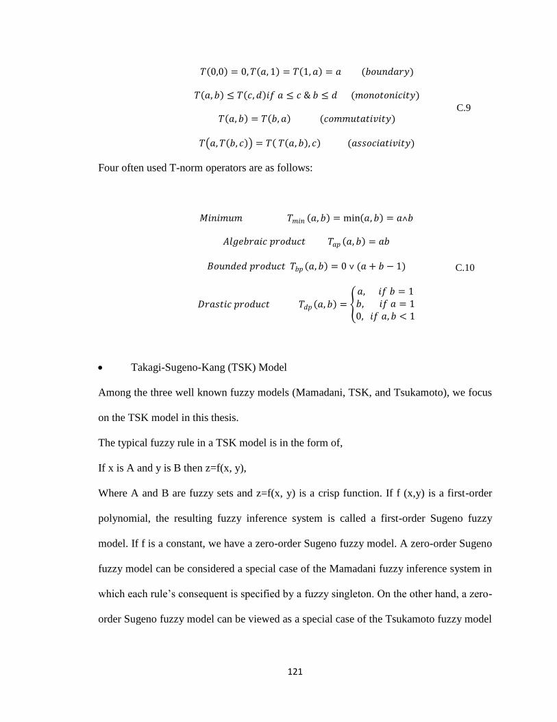
121

𝑇 0,0 = 0, 𝑇 𝑎, 1 = 𝑇 1, 𝑎 = 𝑎 (𝑏𝑜𝑢𝑛𝑑𝑎𝑟𝑦)

𝑇 𝑎, 𝑏 ≤ 𝑇 𝑐, 𝑑 𝑖𝑓 𝑎 ≤ 𝑐 & 𝑏 ≤ 𝑑 (𝑚𝑜𝑛𝑜𝑡𝑜𝑛𝑖𝑐𝑖𝑡𝑦)

𝑇 𝑎, 𝑏 = 𝑇 𝑏, 𝑎 (𝑐𝑜𝑚𝑚𝑢𝑡𝑎𝑡𝑖𝑣𝑖𝑡𝑦)

𝑇 𝑎, 𝑇 𝑏, 𝑐 = 𝑇 𝑇 𝑎, 𝑏 , 𝑐 (𝑎𝑠𝑠𝑜𝑐𝑖𝑎𝑡𝑖𝑣𝑖𝑡𝑦)

C.9

Four often used T-norm operators are as follows:

𝑀𝑖𝑛𝑖𝑚𝑢𝑚 𝑇𝑚𝑖𝑛 𝑎, 𝑏 = min 𝑎, 𝑏 = 𝑎˄𝑏

𝐴𝑙𝑔𝑒𝑏𝑟𝑎𝑖𝑐 𝑝𝑟𝑜𝑑𝑢𝑐𝑡 𝑇𝑎𝑝 𝑎, 𝑏 = 𝑎𝑏

𝐵𝑜𝑢𝑛𝑑𝑒𝑑 𝑝𝑟𝑜𝑑𝑢𝑐𝑡 𝑇𝑏𝑝 𝑎, 𝑏 = 0 ˅ (𝑎 + 𝑏 − 1)

𝐷𝑟𝑎𝑠𝑡𝑖𝑐 𝑝𝑟𝑜𝑑𝑢𝑐𝑡 𝑇𝑑𝑝 𝑎, 𝑏 =

𝑎, 𝑖𝑓 𝑏 = 1𝑏, 𝑖𝑓 𝑎 = 10, 𝑖𝑓 𝑎, 𝑏 < 1

C.10

Takagi-Sugeno-Kang (TSK) Model

Among the three well known fuzzy models (Mamadani, TSK, and Tsukamoto), we focus

on the TSK model in this thesis.

The typical fuzzy rule in a TSK model is in the form of,

If x is A and y is B then z=f(x, y),

Where A and B are fuzzy sets and z=f(x, y) is a crisp function. If f (x,y) is a first-order

polynomial, the resulting fuzzy inference system is called a first-order Sugeno fuzzy

model. If f is a constant, we have a zero-order Sugeno fuzzy model. A zero-order Sugeno

fuzzy model can be considered a special case of the Mamadani fuzzy inference system in

which each rule’s consequent is specified by a fuzzy singleton. On the other hand, a zero-

order Sugeno fuzzy model can be viewed as a special case of the Tsukamoto fuzzy model

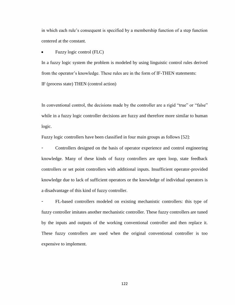
122

in which each rule’s consequent is specified by a membership function of a step function

centered at the constant.

Fuzzy logic control (FLC)

In a fuzzy logic system the problem is modeled by using linguistic control rules derived

from the operator’s knowledge. These rules are in the form of IF-THEN statements:

IF (process state) THEN (control action)

In conventional control, the decisions made by the controller are a rigid “true” or “false”

while in a fuzzy logic controller decisions are fuzzy and therefore more similar to human

logic.

Fuzzy logic controllers have been classified in four main groups as follows [52]:

- Controllers designed on the basis of operator experience and control engineering

knowledge. Many of these kinds of fuzzy controllers are open loop, state feedback

controllers or set point controllers with additional inputs. Insufficient operator-provided

knowledge due to lack of sufficient operators or the knowledge of individual operators is

a disadvantage of this kind of fuzzy controller.

- FL-based controllers modeled on existing mechanistic controllers: this type of

fuzzy controller imitates another mechanistic controller. These fuzzy controllers are tuned

by the inputs and outputs of the working conventional controller and then replace it.

These fuzzy controllers are used when the original conventional controller is too

expensive to implement.

123

- Model based fuzzy control: This type of fuzzy controller uses a given fuzzy open

loop model of a controlled system to derive the set of fuzzy rules. This method, in

contrast to previous types, requires a model of the system.

- Self-learning fuzzy controls: This kind of fuzzy controller is called an adaptive

fuzzy controller. The parameters of adaptive fuzzy controllers are tuned online to provide

the best performance even if the system parameters change over time. For this tuning, the

system data can be used directly or an identifier mechanism can produce a model of the

system.

ANFIS [51]

ANFIS stands for adaptive network-based fuzzy inference system or, semantically

equivalent, adaptive neuro fuzzy inference system. Figure C.9 (a) and (b) show the

reasoning mechanism and architecture of an ANFIS with two inputs and one output. For a

first-order Sugeno fuzzy model, a common rule set with two fuzzy if-then rules is

following:

Rule1: If x is A1 and y is B1, then f1=p1x+q1y+r1,

Rule2: If x is A2 and y is B2, then f2=p2x+q2y+r2,

The reasoning mechanism shown in figure C.9 (a) is a Sugeno model. The nodes of the

same layer have similar functions as described next where O1,i is the output of the ith

node

in layer 1.

- Layer 1:

𝑂1,𝑖 = µ𝐴𝑖 𝑥 𝑓𝑜𝑟 𝑖 = 1,2

𝑂1,𝑖 = µ𝐵𝑖−2 𝑦 𝑓𝑜𝑟 𝑖 = 3,4

C.11

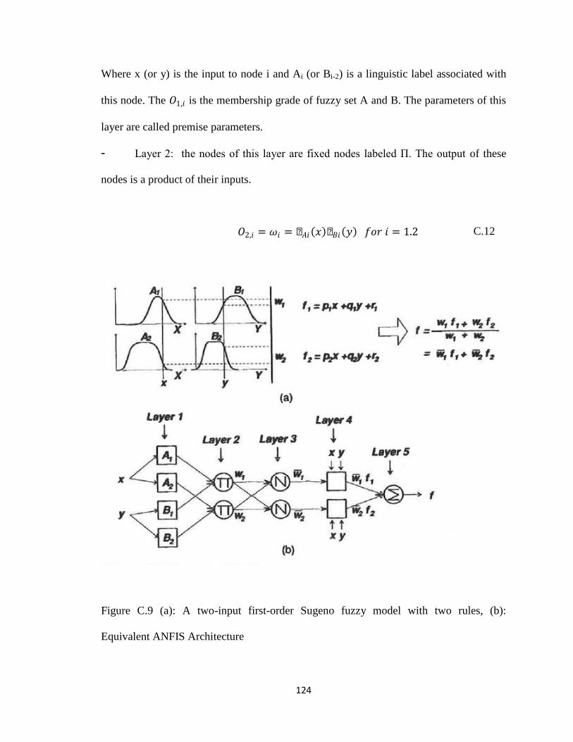
124

Where x (or y) is the input to node i and Ai (or Bi-2) is a linguistic label associated with

this node. The 𝑂1,𝑖 is the membership grade of fuzzy set A and B. The parameters of this

layer are called premise parameters.

- Layer 2: the nodes of this layer are fixed nodes labeled П. The output of these

nodes is a product of their inputs.

𝑂2,𝑖 = 𝜔𝑖 = µ𝐴𝑖 𝑥 µ𝐵𝑖 𝑦 𝑓𝑜𝑟 𝑖 = 1.2 C.12

Figure C.9 (a): A two-input first-order Sugeno fuzzy model with two rules, (b):

Equivalent ANFIS Architecture

125

Any other T-norm operators that perform a fuzzy “AND” can be used instead of

“product” in this layer.

- Layer 3: the nodes of this layer are fixed nodes labelled N. The output of these

nodes is the ratio of the ith

rule’s firing strength to the sum of all rules’ firing strength.

𝑂3,𝑖 = 𝜔𝑖 =𝜔𝑖

𝜔1 + 𝜔2 𝑓𝑜𝑟 𝑖 = 1.2

C.13

The output of this layer is called normalized firing strengths.

- Layer 4: the function of the nodes in this layer is as follow:

𝑂4,𝑖 = 𝜔𝑖 𝑓𝑖 = 𝜔𝑖 (𝑝𝑖𝑥 + 𝑞𝑖𝑦 + 𝑟𝑖) C.14

Where 𝜔𝑖 is a normalized firing strength from layer 3 and 𝑝𝑖 , 𝑞𝑖 , 𝑟𝑖 are parameters of the

nodes.

- Layer 5: the node of this layer is a fixed node labeled Σ. The output of this node is

the overall output calculated as follow:

𝑜𝑣𝑒𝑟𝑎𝑙𝑙 𝑜𝑢𝑡𝑝𝑢𝑡 = 𝑂5,1 = 𝜔𝑖 𝑓𝑖

𝑖

= 𝜔𝑖𝑓𝑖𝑖

𝜔𝑖𝑖 C.15

The nodes of layer 1 and layer 5 are not fixed and can be tuned during the learning

process.

Throughout this thesis, we use the ANFIS architecture for the first-order Sugeno fuzzy

model with two inputs, one output, and 9 rules. Figure C.10 deals with such an ANFIS

architecture.

126

Figure C.10: ANFIS structure with two inputs

Hybrid learning method

The hybrid learning method is used to identify the parameters of adaptive networks. This

method is a combination of a forward pass and a backward pass in which least-squares

estimator (LSE) and steepest decent (SD) are applied respectively. In other words, the

hybrid learning method consists of LSE and SD. The most important advantage of the

hybrid method, in comparison to back propagation and SD, is that this method is faster.

One can divide this method into two main parts: off-line learning (batch learning) and on-

line learning (pattern-by-pattern learning). In this thesis we focus on off-line learning.

The next paragraphs deal with the forward pass and backward pass of the off-line

learning method:

127

- Forward pass:

The output of a one-output adaptive network can be represented by

𝑂 = 𝐹(𝑖, 𝑆) C.16

Where “i” is the vector of input variables, F is the overall function of the network, and S

is the set of network parameters. We assume that: S consists of two sets of S1 (Set of

premise parameters) and S2 (set of consequent parameters, and also there is a function H

such that the composite function H o F is linear in the elements of S2.

Therefore we have,

𝐻(𝑂) = 𝐻𝑜𝐹(𝑖, 𝑆) C.17

Which is linear in elements of S2. Given the values of the elements of S1 and plugging p

training data into equation 3.15 one can obtain a matrix equation in the form of

𝐴𝑋 = 𝐵 C.18

Where x is a vector of parameters S2 and A and B are inputs and outputs respectively.

According to linear least-square problems, the best solution for x which minimizes

𝐴𝑋 − 𝐵 2, is the least-square estimator (LSE) 𝑋∗:

𝑋∗ = 𝐴𝑇𝐴 −1𝐴𝑇𝐵 C.19

Where 𝐴𝑇is the transpose of A.

- Backward pass

After the consequent parameters are identified in a forward pass, the error measure can be

obtained for each training data pair. In backward pass the derivative of the error measure

with respect to each node output propagates from the output end toward the input end. In

backward pass the premise parameters (S1) are updated by steepest descent method.

128

The overall output of the ANFIS structure shown in figure C.9(b) can be represented as a

linear combination of the consequent parameters as follow:

𝑓 =𝜔1

𝜔1 + 𝜔2𝑓1 +

𝜔2

𝜔1 + 𝜔2𝑓2

= 𝜔 1 𝑝1𝑥 + 𝑞1𝑦 + 𝑟1 + 𝜔 2 𝑝2𝑥 + 𝑞2𝑦 + 𝑟2

= 𝜔 1𝑥 𝑝1 + 𝜔 1𝑦 𝑞1 + 𝜔 1 𝑟1 + 𝜔 2𝑥 𝑝2 + 𝜔 2𝑦 𝑞2 + 𝜔 2 𝑟2

C.20

As can be derived from equation C.20, the overall output of the ANFIS can be expressed

linearly in the consequent parameters. If we define S, S1, and S2 as the set of total

parameters, set of premise parameters and set of consequent parameters respectively, the

hybrid rule explained above can be applied.

design, development, and human analogous control...

Documents