design, development, and evaluation of focused …
TRANSCRIPT

The Pennsylvania State University
The Graduate School
Graduate Program in Acoustics
DESIGN, DEVELOPMENT, AND EVALUATION OF FOCUSED ULTRASOUND
ARRAYS FOR TRANSESOPHAGEAL CARDIAC ABLATIONS
A Thesis in
Acoustics
by
Hotaik Lee
© 2006 Hotaik Lee
Submitted in Partial Fulfillment of the Requirements
for the Degree of
Doctor of Philosophy
December 2006

The thesis of Hotaik Lee was reviewed and approved* by the following:
Nadine Barrie Smith Associate Professor of Bioengineering and Acoustics Thesis Advisor Chair of Committee
Victor W. Sparrow Associate Professor of Acoustics
Thomas B. Gabrielson Professor of Acoustics
Keefe B. Manning Assistant Professor of Bioengineering
Anthony A. Atchley Professor of Acoustics Head of the Graduate Program in Acoustics
*Signatures are on file in the Graduate School

ii
ABSTRACT
The ultimate purpose of this dissertation is the evaluation of the feasibility of
transesophageal cardiac surgery in arrhythmia treatment, using therapeutic ultrasound
energy without the requirement for surgical incisions or blood contact.
Atrial fibrillation (AF) is the most common cardiac arrhythmia, affecting over 2.2
million Americans. One effective treatment is cardiac ablation, which shows a high rate
of success in treating paroxysmal AF. As a prevailing modality for this treatment,
catheter ablation using radiofrequency has been effective, but there is measurable
morbidity and significant costs and time associated with this invasive procedure for
permanent or persistent AF. To address these issues, a transesophageal ultrasound
applicator for noninvasive cardiac ablations has been designed, developed and evaluated
in this dissertation. Focused ultrasound for thermal ablation has gained interest for
decades due to its noninvasive characteristics. Since the esophagus is close to the
posterior of the left atrium, its position makes it attractive for the incision-less surgery of
the selected area of the heart using ultrasound. The overall goal of this study is to bring
an applicator as closely as possible to the heart in order to effectively deliver ultrasound
energy, and create electrically isolating lesions in myocardial tissue, replicating the
currently used Maze procedure. The Maze procedure is a surgical operation that treats AF
by creating a grid of incisions resulting in non-conductive scar tissue in the atria.
The initial design of an ultrasound applicator capable of creating atrial lesions
from the esophagus, involved evaluating sound pressure fields within layers of the
esophagus and myocardium. Based on the multiple factors of the simulation results of

iii
transducer arrays, current transesophageal medical devices, and the throat anatomy, a
focused ultrasound transducer that can be inserted into the esophagus has been designed
and tested. In this study, a two-dimensional sparse phased array with flat tapered
elements was found to be adequate as a transesophageal ultrasound applicator. The
spatially sparse array uses 64 active elements operating at a frequency of 1.6 MHz
sampled from 195 (15 by 13) rectangular elements. With this applicator, the size and
position of the ablation targets can be controlled by changing the electrical power and
phase to the individual elements for ultrasound beam focusing and steering. The magnetic
resonance-compatible probe head housing is 19 mm in diameter and incorporates an
acoustic window. For the verification of the suggested design, a prototype array with an
acoustic impedance matching layer was constructed, and tested using exposimetry and ex
vivo experiments. Experimental results indicated that the array could focus and steer the
beam with an angle within ±10° inside the tissue. Also, the array can deliver sufficient
power to the focal point to produce ablation while not damaging nearby tissue outside the
target area. The results demonstrated a potential application of the ultrasound applicator
to transesophageal cardiac surgery in atrial fibrillation treatment.

iv
TABLE OF CONTENTS
LIST OF FIGURES .....................................................................................................vii
LIST OF TABLES.......................................................................................................xii
ACKNOWLEDGEMENTS.........................................................................................xiii
Chapter 1 Introduction ................................................................................................1
1.1 Background and motivations ..........................................................................1 1.2 Specific aims and scope..................................................................................3 1.3 Dissertation outlines .......................................................................................4
Chapter 2 Clinical background ...................................................................................6
2.1 Atrial Fibrillation (AF) ...................................................................................6 2.2 Pulmonary Vein Isolation (PVI).....................................................................9 2.3 Maze procedure ..............................................................................................10 2.4 Energy sources for ablation ............................................................................12
2.4.1 Radiofrequency (RF) ablation ..............................................................13 2.4.2 Cryoablation .........................................................................................14 2.4.3 High-Intensity Focused Ultrasound (HIFU).........................................15
2.5 Anatomy and physiology studies: Heart and esophagus ................................17 2.5.1 Heart .....................................................................................................18
2.5.1.1 Overview ....................................................................................18 2.5.1.2 Heart Wall ..................................................................................19 2.5.1.3 Heart chambers and veins ..........................................................20
2.5.2 Esophagus.............................................................................................22 2.5.3 Relationship between the Heart and Esophagus...................................23
2.6 Transesophageal devices: An example of transesophageal device in clinical application ........................................................................................25
Chapter 3 Ultrasound for thermal treatment ...............................................................27
3.1 Fundamentals of therapeutic ultrasound.........................................................27 3.1.1 Description, brief history, and applications of ultrasound in clinical
field.........................................................................................................27 3.1.2 Applications of therapeutic ultrasound.................................................29 3.1.3 Focused ultrasound surgery (FUS).......................................................32
3.1.3.1 Mechanism of ultrasound surgery ..............................................32 3.1.3.2 Clinical applications...................................................................33
3.2 Ultrasound transducer array............................................................................33 3.2.1 Types of array.......................................................................................34
3.2.1.1 Linear Array ...............................................................................34

v
3.2.1.2 Curved Linear Array ..................................................................35 3.2.1.3 Phased Array ..............................................................................36
3.2.2 Focusing ...............................................................................................37 3.2.3 Sparse array ..........................................................................................39
3.3 Thermal distribution on tissue ........................................................................41 3.3.1 Bio-heat transfer model of tissue..........................................................41 3.3.2 Thermal dose ........................................................................................43
Chapter 4 Array design and numerical analysis .........................................................46
4.1 Acoustic pressure calculations........................................................................46 4.1.1 Rayleigh-Sommerfeld integral .............................................................47 4.1.2 Tupholme-Stepanishen method ............................................................48 4.1.3 Calculation of radiation beam fields.....................................................50
4.1.3.1 Single rectangular transducer .....................................................50 4.1.3.2 Multi-element transducer ...........................................................54
4.2 Ultrasound transducer array design and simulations......................................58 4.2.1 Array designs........................................................................................59
4.2.1.1 Overview ....................................................................................59 4.2.1.2 Array profile with radiation pattern ...........................................60
4.2.2 Periodic sparse phased array ................................................................61 4.2.3 Random sparse phased array ................................................................71 4.2.4 Tapered array........................................................................................74
4.3 Temperature distribution computations..........................................................77 4.3.1 Numerical methods for bio-heat transfer equation...............................77
4.3.1.1 Finite Difference Method (FDM)...............................................77 4.3.1.2 Initial and boundary conditions..................................................79 4.3.1.3 Stability requirement ..................................................................81
4.3.2 Simulations of thermal distribution: Thermal ablation ........................82 4.3.2.1 Introduction ................................................................................82 4.3.2.2 Thermal model of the tissues .....................................................82 4.3.2.3 Computational results and analysis ............................................83
Chapter 5 Transducer probe fabrication .....................................................................87
5.1 Transducer array construction ........................................................................88 5.1.1 Materials for the array ..........................................................................88 5.1.2 Array construction ................................................................................90 5.1.3 Acoustic impedance matching..............................................................92 5.1.4 Cables ...................................................................................................93 5.1.5 Phasing for focusing .............................................................................95
5.2 Electrical matching .........................................................................................96 5.3 Probe housing .................................................................................................97
5.3.1 Housing.................................................................................................97 5.3.2 Acoustic window..................................................................................100

vi
5.4 Water circulation system ................................................................................103
Chapter 6 Experiments for ex vivo evaluation ............................................................105
6.1 Preliminary experiments: Exposimetry ..........................................................105 6.1.1 Introduction ..........................................................................................105 6.1.2 Experimental setup ...............................................................................107 6.1.3 Results and analysis..............................................................................109
6.2 Ex vivo experiments........................................................................................118 6.2.1 Introduction ..........................................................................................118 6.2.2 Experimental setup ...............................................................................119 6.2.3 Results and analysis..............................................................................122
Chapter 7 Conclusions ................................................................................................127
7.1 Summary and conclusions ..............................................................................127 7.2 Suggested future works...................................................................................131
Bibliography ................................................................................................................135
Appendix A Tupholme-Stepanishen method..............................................................143
Appendix B MATLAB program codes for sound fields calculations using a sparse array ...........................................................................................................149

vii
LIST OF FIGURES
Figure 2.1: Illustration of electric system of the heart during (a) normal state, and (b) atrial fibrillation (Morady, 2005)....................................................................7
Figure 2.2: Depiction of abnormal electric system of the heart during atrial fibrillation (left) and blocked abnormal pathways by the encircling lesions on the tissue at the left atrium....................................................................................11
Figure 2.3: Layer of the heart: the heart consists of three main layers – endocardium, myocardium, and epicardium. .......................................................19
Figure 2.4: Illustration of the anatomical relationship between the centers of four PVs ostium and the anterior-posterior average diameters of each ostia, which are electrically isolated for the treatment for AF. R=right, L=left, S=superior, and I=inferior ........................................................................................................21
Figure 2.5: Computed Tomographic analysis of the anatomy of the left atrium and the esophagus (Lemola et al., 2004). Eso=Esophagus; PV=Pulmonary vein.......24
Figure 3.1: A picture of Sonoblate 500® thermal ablation system (Focus Surgery Inc., Indianapolis, IN)...........................................................................................31
Figure 3.2: Sketch of linear array transducer (Jensen, 1999). .....................................34
Figure 3.3: Sketch of curved linear array transducer (Jensen, 1999). .........................35
Figure 3.4: Sketch of phased array transducer (Jensen, 1999). ...................................36
Figure 3.5: Ultrasound beam focusing technique by (a) electronic focusing and (b) an acoustic lens. ....................................................................................................37
Figure 3.6: A sketch of a sparse random array for focused ultrasound surgery (Goss et al., 1996).................................................................................................40
Figure 3.7: Graph of the attenuation coefficient versus frequency (0.5-7 MHz) for mammalian tendon, heart and liver. (Goss et al., 1979) .......................................43
Figure 4.1: Definition of the coordinate axes and a plane rectangular piston for sound pressure calculations. The center of the element defines the origin of the coordinate system and the pressure is calculated at field point, (x0, y0, z0). The z-axis is coincident with the element normal. ...............................................51
Figure 4.2: Numerical results of the ultrasound pressure field of a planar rectangular transducer with 5 × 5 mm2 in size at 1.6 MHz using the Tupholme-Stepanishen method. ...........................................................................52
viii
Figure 4.3: Numerical results of the ultrasound pressure field of a planar rectangular transducer with 5 × 5 mm2 in size at 1.6 MHz using the Rayleigh-Sommerfeld integral. ............................................................................................53
Figure 4.4: Numerical results of the angular response at the far-field of a planar rectangular transducer with 5 × 5 mm2 in size at 1.6 MHz. .................................54
Figure 4.5: Numerical results of a normalized sound intensity map of a linear focused phased array with 32-elements and a wavelength in pitch size at 1.6 MHz using the Rayleigh-Sommerfeld integral ((a) and (c)) and the Tupholme-Stepanishen method ((b) and (d)). (a) and (b) show contours of on-axis focusing at (0, 0, 40) mm and (c) and (d) shows off-axis focusing at (20, 0, 40) mm..............................................................................................................56
Figure 4.6: Numerical and analytical results of the sound radiation pattern at far-field from a linear non-focused phased array with 32-elements and a wavelength in pitch size. (a), (c), and (e) are non-steered. (b), (d), and (f) are steered toward θ =14°. ..........................................................................................57
Figure 4.7: (a) Scheme of the linear phased array (Design #1) and simulation results of the ultrasound field of the normalized intensity for (b) on-axis focusing and (c) off-axis focusing plotted as a contour with levels indicated at 0, -1, -2, -3, -6, -9 and -12 dB,..............................................................................63
Figure 4.8: (a) Scheme of the linear phased array (Design #2) and simulation results of the ultrasound field of the normalized intensity for (b) on-axis focusing and (c) off-axis focusing plotted as a contour with levels indicated at 0, -1, -2, -3, -6, -9 and -12 dB...............................................................................65
Figure 4.9: (a) Scheme of the linear phased array (Design #3) and simulation results of the ultrasound field of the normalized intensity for (b) on-axis focusing and (c) off-axis focusing plotted as a contour with levels indicated at 0, -1, -2, -3, -6, -9 and -12 dB...............................................................................67
Figure 4.10: (a) Scheme of the periodic sparse phased array (Design #4) and simulation results of the ultrasound field of the normalized intensity for (b) on-axis focusing and (c) off-axis focusing plotted as a contour with levels indicated at 0, -1, -2, -3, -6, -9 and -12 dB, as indicated from the intensity color bar. ...............................................................................................................70
Figure 4.11: (a) Scheme of the random sparse phased array (Design #5) and simulation results of the ultrasound field of the normalized intensity for (b) on-axis focusing and (c) off-axis focusing plotted as a contour with levels indicated at 0, -1, -2, -3, -6, -9 and -12 dB, as indicated from the intensity color bar. ...............................................................................................................73

ix
Figure 4.12: (a) Scheme of the tapered phased array with periodically sparsed elements (Design #6) and simulation results of the ultrasound field of the normalized intensity for (b) on-axis focusing and (c) off-axis focusing plotted as a contour with levels indicated at 0, -1, -2, -3, -6, -9 and -12 dB, as indicated from the intensity color bar...................................................................76
Figure 4.13: Boundary conditions for the heat transfer equation in soft tissue at various types of boundaries. (Incropera and De Witt, 1990)................................81
Figure 4.14: Simulation results of (a) temperature as a function of time calculated at the location of the focal point and (b) the thermal distribution within the cardiac tissue (ex vivo with peak sound intensity at the focal point of 50 W/cm2). .................................................................................................................85
Figure 4.15: Simulation results of (a) temperature as a function of time calculated at the location of the focal point and (b) the thermal distribution within the cardiac tissue (in vivo with peak sound intensity at the focal point of 70 W/cm2). .................................................................................................................86
Figure 5.1: A diagram showing a back view of the 15-by-13 linear tapered array with total size of 20.70 × 10.24 mm2. The diced face of the ceramic was completely cut through its thickness. An enlarged representation of the elements shows that the distance between the adjacent elements is 105 µm, which represents the thickness of the cutting blade. ............................................91
Figure 5.2: The photograph of the prototype array after dicing into 15-by-13 elements including 64 active elements periodically sparse. .................................92
Figure 5.3: The photograph showing the back view of transducer array with coaxial cables........................................................................................................95
Figure 5.4: Photograph of one of 16 matching circuit boards for the prototype array. One circuit board includes 4 channel matching circuits.............................97
Figure 5.5: 3-D CAD SolidWorks® drawing of the housing prototype.......................99
Figure 5.6: Illustrations of the refraction of the ultrasound ray due to the acoustic window .................................................................................................................100
(Water: Z = 1.5 MRayls, c = 1500 m/s; TPX®: Z = 1.78 MRayls, c = 2170 m/s; Tissue: Z = 1.5 MRayls, c = 1500 m/s) ................................................................100
Figure 5.7: Simulation results of the refracted angle at the outer surface of the housing according to the heights (h1) of the transducer array elements. .............101

x
Figure 5.8: Illustration of the resulting ultrasound rays due to the refracted ultrasound beam for the different thickness of the windows................................102
Figure 5.9: Photograph of the assembled probe head with water circulation tubes ....103
Figure 5.10: Photograph of the constructed transesophageal ultrasound applicator with the insertion tube including cables inside, the ZIF connector, and water circulation tubes....................................................................................................104
Figure 6.1: Experimental apparatus for exposimetry. The array and hydrophone are held in a water tank.........................................................................................106
Figure 6.2: Schematic diagram of the experiment setup used in exposimetry measurement of the sound pressure field from the ultrasound array....................108
Figure 6.3: Exposimetry results of the ultrasound field of the temporal peak intensity for on-axis focusing with the focal point aimed at (0, 0, 30) mm with the prototype array (n=1)..............................................................................110
Figure 6.4: Exposimetry results of the ultrasound field of the temporal peak intensity for off-axis focusing with the focal point aimed at (-5, 0, 30) mm with the prototype array (n=1)..............................................................................111
Figure 6.5: Exposimetry results of the ultrasound field of the temporal peak intensity for on-axis focusing either with or without the acoustic window attached to the probe housing (n=1). ....................................................................112
Figure 6.6: Exposimetry results of the lateral responses for on-axis focusing with the focal point aimed at (0, 0, 30) mm with the prototype array. The input driving powers are 0.5-2.0 W/channel and the sound intensities were measured at the maximum pressure point (n=1)...................................................114
Figure 6.7: Comparison of the results between exposimetry and numerical simulation of the ultrasound field of the temporal peak intensity for on-axis focusing with the focal point aimed at (0, 0, 30) mm with the prototype array (n=4). ....................................................................................................................115
Figure 6.8: Comparison of the results between exposimetry and numerical simulation of the ultrasound field of the temporal peak intensity for off-axis focusing with the focal point aimed at (-5, 0, 30) mm with the prototype array (n=4). ....................................................................................................................115
Figure 6.9: Exposimetry results of the ultrasound field of the temporal peak intensity, as indicated from the intensity color bar, for on-axis focusing with (b) the focal point aimed at (0, 0, 30) mm in xy-plane, (c) in xz-plane, and
xi
(d) for off-axis focusing with the focal point aimed at (-5, 0, 30) mm in xy-plane with the prototype array. .............................................................................117
Figure 6.10: Distribution plot of the median temperature associated with excitability and tissue injury (Nath et al., 1993) ..................................................119
Figure 6.11: Schematic diagram of the experimental setup for ex vivo thermal ablation using the ultrasound phased array...........................................................121
Figure 6.12: Temperature as a function of time recorded at the location of the focal point. The temperature rose from 37 °C to 50 °C for two minutes and then remained over 50°C for three minutes..........................................................122
Figure 6.13: (a) Schematic diagram of ex vivo thermal ablation by the ultrasound array for on-axis focusing in the rat liver. (b) Photograph of the rat liver showing a lesion generated by on-axis focusing at (0, 0, 30) mm. The lesion (arrow) had dimensions of 6 × 3 × 3 mm3 and was generated by five-minute exposure................................................................................................................123
Figure 6.14: Photograph of an ex vivo experimental result showing a lesion generated by on-axis focusing at (0, 0, 30) mm. The lesion (arrow) in porcine heart has dimensions of 6 × 5 × 5 mm3 and was generated by eight minutes exposure (small photograph: top view). ...............................................................125
Figure 6.15: Photograph of an ex vivo experimental result showing a lesion generated by on-axis focusing at (0, 0, 25) mm. The lesion in the endocardium has dimensions of 4 × 3 mm2 and was generated by eight minutes exposure. .................................................................................................126
Figure A.1: Positions of aperture, field point, and coordinate system (Jensen, 1999). ....................................................................................................................143
Figure A.2: Definition of distances and angles in the aperture plane for calculating the spatial impulse response (Jensen, 1999). ........................................................146

xii
LIST OF TABLES
Table 4.1: A summary of the design parameters of linear phased array designs and the outputs from the sound field simulations........................................................68
Table 4.2: Physical parameters used in acoustic calculations and biothermal simulations............................................................................................................83
Table 5.1: Comparison of the properties between piezoelectric ceramics. .................89

xiii
ACKNOWLEDGEMENTS
The completion of this dissertation was made possible through the support of
many individuals. First and foremost, I would like to express my deepest gratitude to my
advisor and committee chair, Dr. Nadine Smith. Throughout my time at The Therapeutic
Ultrasound Applications Laboratory, she has been a great support for me in every aspect.
She has offered me guidance, encouragement as well as constructive criticism, and for
that I will be eternally grateful to her.
I also extend an expression of special thanks to my doctoral committee, Dr. Victor
Sparrow, Dr. Thomas Gabrielson, and Dr. Keefe Manning, for their insightful
suggestions on this dissertation. I have also become indebted to Dr. Anthony Atchley,
head of The Graduate Program in Acoustics, for his guidance and support of my doctoral
studies, and Dr. Jae-Eung Oh, my former advisor in Korea, who have motivated and
guided me in my professional development.
There are wonderfully supportive people throughout my program and the course
of this study, especially Karen Brooks, Carolyn Smith, Gene Gerber, Dr. Jacob Werner,
Terry Kling, David Francischelli, and Sylvia Hopkins for their great support. I would also
like to thank my colleagues in The Acoustics Program and The Bioengineering
Department, Geon-Seok Kim, Kiwon Jung, Yongsin Hwang, Eun-Joo Park, Justin Kao,
and Yada Juntarapaso, for their moral support and friendship.
More specifically, I dedicate this dissertation to my parents and parents-in-law.
This achievement was possible due to their sacrifices and endless love. Finally, I am so
grateful to my wife, Hyunju and our lovely child, Yewon, who have been extremely
patient with an often-absent husband and dad. They have provided me with the joy and
richness in my life and motivated all of my works at Penn State.

Chapter 1
Introduction
1.1 Background and motivations
Atrial fibrillation (AF) is the most common cardiac arrhythmia, affecting over 2.2
million Americans (Thom et al., 2006). It is one of the most serious public health
problems in the United States, but continues to be an unmet medical need. One effective
treatment is cardiac ablation, which shows a high rate of success in treating paroxysmal
AF. As a prevailing modality, catheter ablation using radiofrequency remains the
treatment of choice however there is measurable morbidity and significant costs and time
associated with this invasive procedure for permanent or persistent AF (Jais et al., 2003).
There is a demand for alternative improved treatment protocols to be made available and
so demands for noninvasive cardiac ablation have increased.
Ultrasound energy has gained interest for clinical applications for decades due to
its noninvasive characteristics. It is widely used in medicine for therapeutic purposes as
well as for diagnostics as it allows the imaging of the inside of the body without the
possible danger from radiation. Ultrasound is essentially different from many other forms
of energy, such as X-rays, radiofrequency or microwave, in its absorptive interactions
between the wave and the medium. Thus it penetrates through intervenient tissue to
deliver heat and mechanical energy to a targeted area without undesirable effects on that
tissue. The feasibility of using focused ultrasound for tissue ablation has been

2
investigated since the early 1980s (Goss et al., 1996;Sanghvi et al., 1997;Smith and
Hynynen, 1998). Specifically for cardiac tissue, surgical studies using the catheter-based
ultrasound transducers for the treatment of arrhythmias have been reported (Zimmer et
al., 1995;Gentry and Smith, 2004;Wong et al., 2004).
Therapeutic ultrasound technology has continued to evolve as a potential
therapeutic tool since the first clinical experience with high intensity focused ultrasound
(HIFU) to treat tissue in the central nervous system was reported in the 1950s (Fry et al.,
1954). In this study, the researchers created lesions deep in brains of cats and monkeys
using ultrasound and demonstrated that absorption of the high intensity pressure waves
elevated local tissue temperature. In addition to the high-intensity ultrasound, the use of
low-intensity ultrasound to enhance the healing process of the tissue by improving
general physiological responses was also explored. Several studies have been reported
that use pulsed, lower-intensity ultrasound energy on bone and cartilage tissues to
produce a number of beneficial physiological effects including increased blood flow and
nutrient delivery to tissues around the target non-invasively (Dyson and Brookes,
1983;Heckman et al., 1994). Recently, the medical application of the therapeutic
ultrasound has been extended to the treatment of benign prostatic hyperplasia (Foster et
al., 1993), lithotripsy with capacity to precisely reach a target (Coleman et al., 1996),
noninvasive transdermal drug delivery (Smith et al., 2003), and focused ultrasound
hemostasis of injured, solid organs (Vaezy et al., 1998). Also recent clinical advances in
HIFU include focused ultrasound surgery (FUS) as a noninvasive alternative to open
surgery (Melodelima et al., 2005;Yin et al., 2006).

3
1.2 Specific aims and scope
The purpose of this dissertation is to evaluate the feasibility of transesophageal
cardiac surgery in atrial fibrillation treatment, using therapeutic ultrasound energy
without surgical incisions or blood contact. This work constitutes the design,
development, and evaluation of focused ultrasound applicators capable of creating
thermal lesions in myocardium from the location of the esophagus. Since the esophagus
is close to the posterior of the left atrium, this position makes it attractive for the incision-
less surgery of the selected areas of the heart.
For the focused ultrasound ablation, the transducer design is a two-dimensional
phased array operating at a frequency of between 1~2 MHz. Either ultrasound pressure
fields or thermal distribution within tissues are numerically simulated for the design of
ultrasound arrays. With this applicator, the size and the position of the ablation targets
can be controlled by changing the electrical power and phase to suit the individual
elements for ultrasound beam focusing and steering. The magnetic resonance-compatible
probe head housing should protect the esophagus from any potential failure of the
transducers. Also the probe incorporates an acoustic window within the housing to ensure
the delivery of maximum acoustical power from the transducers to the ablation targets.
The overall goal is to bring an applicator as closely as possible to the heart in order to
effectively deliver ultrasound energy, and create electrically isolating lesions in
myocardial tissue and allow replication of the currently used Maze procedure.
Based on the multiple factors of numerical simulation results of transducer arrays,
current transesophageal medical devices, and throat anatomy, a focused ultrasound

4
transducer that is insertable into the esophagus for cardiac ablation was designed and
fabricated. To verify the suggested design, a prototype array with an acoustic impedance
matching layer was constructed, and tested using exposimetry and ex vivo experiments.
The exposimetry was used to verify the capability of the ultrasound transducer for
focusing and steering. Also, ex vivo experiments using fresh tissue were used to ensure
that the array is capable of delivering sufficient acoustical power to create lesions in
tissue. Precise control of beam forming on- and off-axis was demonstrated without
significant near-field heating and grating lobes, which have the possibility of causing
undesirable side effects during treatment.
1.3 Dissertation outlines
The brief outline of this dissertation is as follows. Chapter 2 provides relevant
clinical background information such as cardiac arrhythmia, atrial fibrillation-related
treatment, fundamental anatomy and physiology studies on the heart and the esophagus,
and an example of the clinical application of a transesophageal device. Chapter 3 presents
the fundamentals of therapeutic ultrasound and its use for thermal treatment and
ultrasonic transducer array. Included in the discussions of therapeutic ultrasound are high
intensity focused ultrasound for clinical applications, various types of ultrasonic
transducer arrays, and bio-heat transfer model of tissue. Chapter 4 provides results of the
numerical simulations used for the acoustic pressure calculations, design of the
ultrasound phased array, and thermal distribution on the cardiac tissue model. Chapter 5
describes the array construction that includes dicing the piezoelectric ceramic, building

5
the matching layers, wiring the elements and building the matching circuits. In addition,
it discusses the design and fabrication of probe head housing as well as acoustic windows
attached on the housing. Chapter 6 presents the instrumentation and the process used for
the exposimetry. The results from the preliminary tests are compared with the simulation
results and ex vivo experiments. The experimental results are used to evaluate the design
of the ultrasound applicator as well as the feasibility of creating lesions in tissues. Finally,
Chapter 7 provides the conclusions drawn from this research. It also discusses the
research in the context of current therapies and summarizes the findings concerning the
innovative design of a transesophageal ultrasound applicator for noninvasive cardiac
ablations. The chapter concludes with suggestions about possible future research
directions.

Chapter 2
Clinical background
This chapter describes the research rationale by examining the background
information on a cardiac disease and current treatment issues relevant to the scope of this
research. A brief review of atrial fibrillation, existing treatment methods and the need for
improvement are presented. The existing types of energy sources for tissue ablation are
discussed and the concept of thermal ablation using these energy sources is explained.
The basic anatomy and physiology of the heart and esophagus involved in the
transesophageal treatment are also presented.
2.1 Atrial Fibrillation (AF)
Atrial Fibrillation (AF) is a common arrhythmia, in which the atria (upper
chambers of the heart) beat extraordinarily fast and the rhythm disturbance is irregular
and somewhat chaotic. The heart has an electrical system, in which the electrical impulse
from a group of cells, called the Sinoatrial (SA) node, travels in an orderly way through
the heart to the Atrioventricular (AV) node causing the muscle of the heart to contract. In
atrial fibrillation, however, many irregular impulses arise from other parts of the atria and
spread through the atria to the AV node, causing a rapid and unexpected heartbeat.
Ultimately, this irregular condition of atrial contraction reduces the ability of the atria to
pump blood into the ventricles (lower chambers of the heart) and increases the chance of

7
(a) Electric signal flow during the normal
(b) Electric signal flow during the irregular heartbea
Figure 2.1: Illustration of electric system of the heart durinatrial fibrillation (Morady, 2005)
Left atrium
heart
t (atri
g (a)
Left ventricleSinus node
Right ventricle
Right atrium
AV node
beat
s
Sinus node
Right atrium
eAV node
Right ventricle
Left ventricl
Left atrium
Pulmonary vein
Atrial fibrillation impulsesal fibrillation)
normal state, and (b)

8
getting cardiovascular diseases or lung diseases. Figure 2.1 shows the electrical systems
of the heart during the normal heartbeat and an atrial fibrillation (Morady, 2005).
AF is one of the most serious public health problems in the United States. Even
though most are not life threatening and arrhythmia can be more of an annoyance than
anything else, the biggest concern is that AF is responsible for about 15–20% of all
strokes and this may result in heart failure and death (Go et al., 2001). In the United
States, the number of people currently diagnosed with atrial fibrillation is approximately
2.2 million (Thom et al., 2006). Currently it is estimated that almost 6% of people over
65 years of age suffer from AF and the incidence of developing it increases with age
(Atrial Fibrillation Foundation, 2002). The prevalence and the cost for the treatment of
AF are expected to increase continuously over the next several decades, as the percent of
population aged 65 years and over increases.
For the medical treatment and prevention of AF, several approaches are used to
restore stable heart rhythm and to control of heart rate. Medications are the most common
initial treatment used to decrease the rapid heart rate associated with AF. Anti-arrhythmic
drugs delivered through a tube into a vein in the patient's arm can sometimes improve the
normal rhythm of the heart.
When medication doesn't improve symptom control other treatments such as
electrical cardioversion may be used. This approach delivers an electric shock to the chest
through electrodes to recover the fast and irregular heartbeat and has been shown to be
successful in managing some cases of AF. Similarly, atrial pacemakers can be implanted
internally to monitor and regulate the heart rhythm with electrical impulses. Currently the
pacemaker is widely used for the treatment of AF. Several drawbacks, however, have

9
been discovered with internal cardioversion. A clot in a vein, infection, or signals
delivered by the device in error can cause malfunction or failure in the management of
AF.
For the more permanent treatment of AF, cardiac ablation to interrupt abnormal
electrical pathways or abnormal electric signals, which induce AF, may be effective. In
this procedure, a thin and flexible catheter is introduced to the heart muscle through a
blood vessel. Generally radiofrequency (RF) energy has been used to destroy tissue
giving rise to the abnormality in the heart rhythm.
2.2 Pulmonary Vein Isolation (PVI)
One of the non-medication treatments of atrial fibrillation is the procedure of
Pulmonary Vein Isolation (PVI), also called pulmonary vein ablation. As blood vessels
that transport oxygenated blood from the lungs to the left atrium, the four pulmonary
veins (PV) may be important sources of the abnormal electric signals that cause AF. The
right and left superior and inferior pulmonary veins have narrow bands of muscle cells at
each opening to the left atrium. In AF, the bands may start to rapidly generate electric
impulses and this electric discharge may induce AF. The anatomical isolation of PV is an
option for the treatment of AF by confining electric triggers within PV. During PVI using
radiofrequency ablation, which is one well-known technique, the band of muscle cells is
ablated by the energy delivered through a catheter inserted into the blood vessels of the
atrium.
10
The PVI technique is a relatively recently developed procedure. The first report of
successful ablation using radiofrequency energy for AF in humans was published by
Haissaguerre and his colleagues in 1994. They demonstrated the treatment of AF using
linear atrial lesions created by catheter-based radiofrequency energy. More recent studies
have suggested that most AF signals (< 90%) are generated in the four pulmonary veins
(Haissaguerre et al., 1998;Schmitt et al., 2002). Thus, this procedure may effectively
block and isolate the electric impulses fired from the band to the left atrium and hence
prevent the initiation of AF. Although there are several known risks of PVI, such as
narrowing of the openings of the PVs (Saksena and Madan, 2003) and damage to the
phrenic nerve (Cummings et al., 2005), PVI procedure for patients with AF is
recommended as the most effective treatment and is becoming more widely practiced and
accepted (Scheinman and Morady, 2001;Ellenbogen and Wood, 2003).
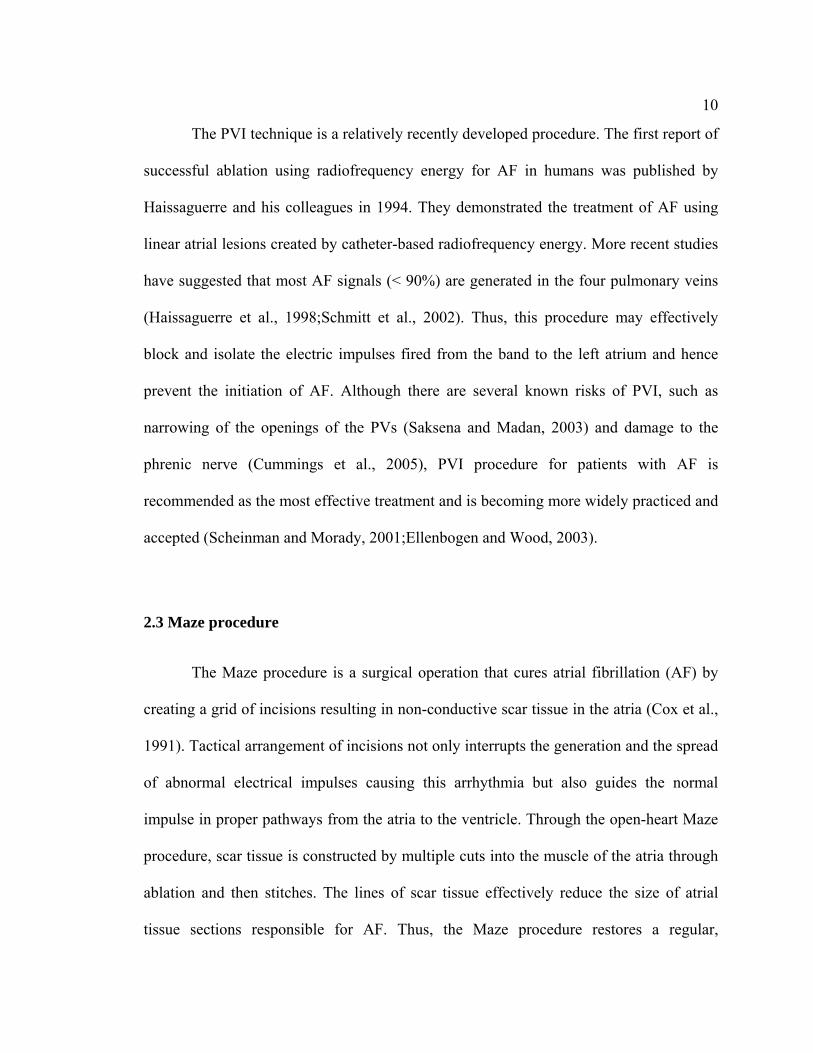
2.3 Maze procedure
The Maze procedure is a surgical operation that cures atrial fibrillation (AF) by
creating a grid of incisions resulting in non-conductive scar tissue in the atria (Cox et al.,
1991). Tactical arrangement of incisions not only interrupts the generation and the spread
of abnormal electrical impulses causing this arrhythmia but also guides the normal
impulse in proper pathways from the atria to the ventricle. Through the open-heart Maze
procedure, scar tissue is constructed by multiple cuts into the muscle of the atria through
ablation and then stitches. The lines of scar tissue effectively reduce the size of atrial
tissue sections responsible for AF. Thus, the Maze procedure restores a regular,

11
coordinated heartbeat and protects the normal contraction of the heart. Figure 2.2 shows
abnormal electric system of the heart during atrial fibrillation (left) and blocked abnormal
pathways by the encircling lesions on the tissue at the left atrium (right).
Copyright © 2001-2006 Mayo Foundation for Medical Education and Research. All rights reserved.
Figure 2.2: Depiction of abnormal electric system of the heart during atrial fibrillation (left) and blocked abnormal pathways by the encircling lesions on the tissue at the left atrium.
Compared to pulmonary vein isolation (PVI), a non-surgical procedure using
catheters, the Maze procedure is usually performed by open-heart surgery requiring
cardiopulmonary bypass during the surgery and invasive method of ablation.

12
Accordingly, it is therefore associated with a risk of surgical complications, such as
bleeding, stroke, kidney failure, other organ failure, and death. The risk of this procedure
is known to be low in general, but the risk will be affected by each individual’s specific
health conditions or age. Although PVI alone is much less effective, it has been
incorporated as an essential component of the Maze procedure.
Due to its complexity, unless the patient is undergoing open-heart surgery for
another condition, such as for repair or replacement of a diseased heart valve, a Maze
surgical procedure for the treatment of AF is not usually recommended. Instead, the
Maze procedure using catheters inside the heart that are introduced through a vein in the
groin without open-heart surgery is the preferred treatment regime. This less surgically
invasive intervention is termed the minimal access catheter Maze procedure, and is
modeled on the surgical Maze procedure. Unsatisfactorily, the success rate using the
catheter-based approach is below 50% and complications such as strokes may occur
(Gaita et al., 2001). Thus, new technologies of non-surgical and minimally invasive
treatment for the AF have been explored and applied with innovative use of various types
of energy source for cardiac ablation.
2.4 Energy sources for ablation
Besides the traditional method to create lesions on cardiac tissue with “cut and
sew”, there are several types of energy source available for surgical treatment by the
Maze procedure and PVI. A number of energy sources including cryoablation,
radiofrequency, microwave, laser, and focused ultrasound, have been introduced to
13
expedite the creation of electrically isolating lesions or scarring localized to the atria.
Most of the energy sources complete the ablation by increasing tissue temperature to
around 50°C and necrosing tissue near the source of the arrhythmia. These advanced
technologies lead the rapid progress in the field of arrhythmia surgery. The fundamental
description and theory on currently available energy sources for ablation of cardiac tissue
are given in this section so as to compare the characteristics of each energy source and
seek better understanding of cardiac ablation for AF.
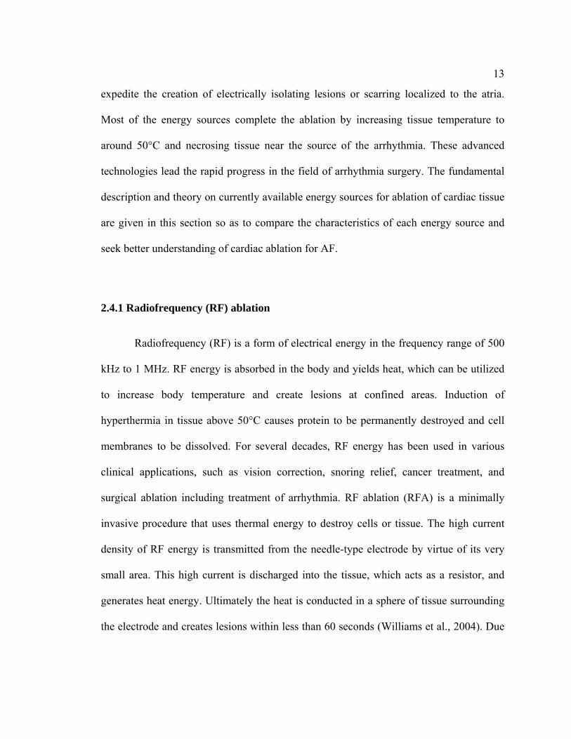
2.4.1 Radiofrequency (RF) ablation
Radiofrequency (RF) is a form of electrical energy in the frequency range of 500
kHz to 1 MHz. RF energy is absorbed in the body and yields heat, which can be utilized
to increase body temperature and create lesions at confined areas. Induction of
hyperthermia in tissue above 50°C causes protein to be permanently destroyed and cell
membranes to be dissolved. For several decades, RF energy has been used in various
clinical applications, such as vision correction, snoring relief, cancer treatment, and
surgical ablation including treatment of arrhythmia. RF ablation (RFA) is a minimally
invasive procedure that uses thermal energy to destroy cells or tissue. The high current
density of RF energy is transmitted from the needle-type electrode by virtue of its very
small area. This high current is discharged into the tissue, which acts as a resistor, and
generates heat energy. Ultimately the heat is conducted in a sphere of tissue surrounding
the electrode and creates lesions within less than 60 seconds (Williams et al., 2004). Due

14
to an obvious boundary between the scar tissue and its surroundings, RF ablation enables
a surgical operation with a high level of precision.
Currently, RFA is widely used to treat some types of arrhythmia, such as AF. The
RF energy burns and necroses the atrial tissue that is responsible for generating or
delivering the signals responsible for the rapid and irregular heartbeats. With the RFA
signal, first the area that is suspected to produce the abnormal electrical impulses is
identified. Once the responsible tissue is mapped, a catheter-based electrode is placed at
the isolated tissue and RF energy is emitted to burn the tissue and block the source of the
impulses. However, like any invasive procedure, RFA carries some associated risks and
potential complications such as pulmonary vein stenosis and stroke. Since RF energy
gives rise to the heat that not only creates lesions on the tissue but can also lead to the
formation of clots, these may induce cerebral stroke by traveling to the brain.
2.4.2 Cryoablation
Cryoablation is a minimally invasive, non-surgical procedure that uses extremely
low temperatures to ablate the tissue and has been used in clinical applications for
instance, prostate cancer, breast cancer, liver tumor, as well as cardiac tissue responsible
to arrhythmia. The prefix “Cryo” derived from the Greek word “Kryos” means cold.
Cryoablation generally uses liquid nitrogen or compressed argon gas to freeze a particular
organ or tissue and create lesions on that area. Using a cryoablation probe, the potential
ablation spots are electrophysiologically examined by instantly freezing the tissue. This is
called cryomapping and is a potentially reversible process. This procedure enables the

15
precise tissue area to be located and targeted for treatment. In cryoablation the tissue
destruction is postponed until the tissue freezes for more than 30 seconds at a temperature
of around -30°C. Thus the lesions are mapped by applying cryoablation to the tissue for
less than 30 seconds and then created by lowering the temperature and maintaining it for
longer time. This is not available when using RF, due to RF’s immediate destruction of
tissue cell.
For the treatment of AF, a portion of the cardiac muscle, which is suspected to
generate or spread abnormal electrical impulses, is examined and frozen by the catheter-
based cryoablation. The area is first tested by lowering the catheter tip to -30°C for
cryomapping, and then dropped the temperature to -75°C to make the cryoablation
permanent. A lesion able to block the abnormal electric signals can be created in
approximately 240 seconds (Friedman et al., 2004) and this treatment regime can be
continued until the arrhythmia disappears. The general commercial system has a variable
length catheter with a catheter tip inserted into the target sites in the left atrium. The other
advantages of using cryoablation include: no damage to the endocardium, the ability to
produce larger and deeper lesions, it is less painful than RF ablation.
2.4.3 High-Intensity Focused Ultrasound (HIFU)
High-intensity focused ultrasound (HIFU) is a noninvasive surgical treatment,
which is a relatively modern technology that seen rapid advancement in recent years (Fry
et al., 1954). HIFU is the clinical application of ultrasound to achieve either a surgical
procedure without an incision or hyperthermia for the treatment of cancers, such as breast

16
cancer, prostate cancer, and renal tumors. Ultrasound energy is delivered to a discrete
area passing through an organ wall structure within the body. The energy absorbed in the
body is transferred to heat energy to create a rise in temperature. The intensive thermal
energy within a well-defined zone ablates the cancerous tissue or the tissue within the
focal area, creating highly localized lesions.
In thermal ablation, high intensity (generally 500 to 1500 W/cm2) ultrasound in
the frequency range of 0.5 to 10 MHz is focused on a targeted area to produce
irreversible tissue necrosis (ter Haar, 1995). Significant lesions are typically achieved at
an exposure of 5 to 15 seconds, and high temperatures up to 60 to100°C (Chen et al.,
1997). The focusing is accomplished by a lens, a concave transducer, or a phased array.
Therapeutic performance is greatly enhanced through an imaging modality, such as
ultrasound imaging and magnet resonance imaging (MRI), to guide and monitor the
procedure. The control of heating using HIFU is precise and effective. It defines the
ablative area in the order of 1–10 mm (Szabo, 2004) so as that HIFU energy enables
consistent and reliable treatment of a number of conditions.
Recent pre-clinical studies have reported the feasibility of HIFU for cardiac
ablation including the treatment of arrhythmia (Zimmer et al., 1995;Smith and Hynynen,
1998). These studies have evaluated the effectiveness of ultrasound for producing lesions
on the atria with the various exposure parameters, such as frequency, intensity amplitude,
focal depth, and exposure time respectively. The technology is evolving, and research is
currently being undertaken on the feasibility of cardiac treatment by a minimally invasive
approach that does not require open surgery. The main advantage of HIFU ablation is that

17
HIFU damages the focused areas of tissue without affecting surrounding tissues or blood
vessels, and may permit treatment of AF without cardiopulmonary bypass.
Ultrasound in conjunction with thermal ablation (local hyperthermia) will be
discussed in more detail in the next chapter.
Other than the energy sources described above, there are additional alternative
sources for surgical atrial ablation including microwave sources and lasers, some of
which have already been approved for clinical use. Microwave ablation performed using
electromagnetic radiation with frequency at 2.5 GHz enables the creation of deeper
lesions than with RF in the same treatment time. Laser energy using a diode laser catheter
that is designed to perform precise microsurgery is currently utilized for Transmyocardial
Revascularization (TMR) and has been investigated as an innovative operation technique
reducing the risks associated with the conventional Maze procedure (Williams et al.,
2004).
2.5 Anatomy and physiology studies: Heart and esophagus
In order to better understand the transesophageal cardiac ablation relevant to this
thesis, it may be helpful to look into the anatomy and physiology of the heart and the
esophagus. Anatomy is the study of the makeup of the body and the relationships
between body structures, and physiology is related to the functions of the body parts. In
this thesis, only the fundamental knowledge of the structures and functions of the heart
and the esophagus is considered.

18
2.5.1 Heart
2.5.1.1 Overview
The mammalian heart is a hollow, muscular organ with four chambers consisting
of the right and left atria and right and left ventricles. In the human body, the heart
normally lies slightly to the left of the middle of the thorax (chest), immediately below
the sternum (breastbone). In the average adult, the heart is about five inches long and
about two and one half inches thick, and weighs about nine to eleven ounces. The heart is
located in the portion of the chest cavity known as the mediastinum, which also includes
the great vessels, the esophagus and other structures. It is enclosed by a fibroserous sac
known as the pericardium and surrounded by loose connective tissue that is often used to
link the surface of the organ to other parts of the organ wall.
The primary function of the heart is to circulate blood through the body. The two
atria operate as collecting containers for blood returning to the heart while the two
ventricles operate as pumps to discharge the blood to the body. Deoxygenated blood
(from the body) is pumped through the right atrium and the right ventricle (to the lungs),
while oxygenated blood (from the lungs) is pumped through the left atrium and the left
ventricle (to the body). The oxygenated blood is carried to the left atrium via pulmonary
veins in which most of the abnormal electrical signals in atrial fibrillation are generated.

19
2.5.1.2 Heart Wall
For cardiac ablation using ultrasound, it is very important to identify the
properties of the heart wall because the ultrasound energy is delivered to a targeted area
passing through the heart wall structure within the body. As shown in Figure 2.3, the
heart consists of three layers – endocardium, myocardium, and epicardium – and is
enwrapped in a fourth protective layer known as the pericardium.
The endocardium is the name given to the inside lining of the heart wall. Because
it directly contacts with the blood in the chambers, the diffusive effect on the thermal
distribution over the heart wall should be carefully considered during the ultrasonic
treatment.
Figure 2.3: Layer of the heart: the heart consists of three main layers – endocardium, myocardium, and epicardium.

20
The myocardium (heart muscle) varies in thickness and constitutes the bulk of the
heart, controlling its contraction and relaxation of the heart. Experimental studies have
suggested that an electrophysiological change of the atrial myocardium is one of the
underlying mechanisms responsible for the occurrence and maintenance of arrhythmia
(Wijffels et al., 1995).
The epicardium forms the inner section of the double walled sac enclosing the
heart as well as providing an outer protective layer for the heart. It is attached to the
myocardium by loose connective tissue. According to recent clinical update, the
epicardial ablation of AF using HIFU may be effectively performed without introducing
the potential risks of endocardial RF ablation, such as esophageal fistula and pulmonary
vein stenosis (Cox, 2005).
Lastly, the elastic tissue layer that constitutes the outer portion of the fluid filled
sac is called the pericardium. It keeps the heart contained in the chest cavity and prevents
the heart from over-expanding when blood volume increases. The pericardial cavity
between the epicardium and the pericardium is filled with pericardial fluid, which acts as
a shock absorber by moderating conflict between the pericardial membranes.
2.5.1.3 Heart chambers and veins
The heart is divided into two sides, the left and the right, by the septum and each
half of the heart is divided into an upper chamber and a lower chamber. The upper
chambers are called atria and the lower chambers are called ventricles. The left atrium
pumps oxygenated blood from the lungs into the left ventricle, which discharges the

21
blood out of the heart to the body through the aorta. The right atrium receives
deoxygenated blood from the body and moves it to the right ventricle, which pumps the
blood out of the heart via the pulmonary arteries to the lungs for gas exchange. A special
cluster of cells (Sinoatrial node) regulating the heart rate is situated in the right atrium,
and the pulmonary veins (PVs) in which rapid rhythms often arise during AF are located
in the left atrium. The average thickness of the posterior left atrium is 2.2 ± 0.9 mm,
ranging from 0.9 to 7.4 mm (Lemola et al., 2004). The average distances between the
centers of the four PVs ostium and the anterior-posterior average diameters of each ostia,
which are electrically isolated for the treatment for AF, are illustrated in Figure 2.4,
respectively (Kato et al., 2003).
RSPV LSPV
RIPV LIPV
Left Atrium
47.2±5.8 mm
41.6±7.3 mm
7.4±3.4 mm 10.5±2.1 mm
Φ13.0±2.5 mm Φ12.4±3.1 mm
Φ9.9±2.6 mm Φ14.1±2.1 mm
Figure 2.4: Illustration of the anatomical relationship between the centers of four PVs ostium and the anterior-posterior average diameters of each ostia, which are electrically isolated for the treatment for AF. R=right, L=left, S=superior, and I=inferior

22
2.5.2 Esophagus
In the human body, the esophagus is a muscular tube that connects the pharynx to
the stomach, located in the thorax behind the trachea and on the right side of the aorta
through the posterior mediastinum, around 25 cm long and 2.5 cm in diameter. The
average thickness of the anterior side of the esophageal wall adjacent to the posterior left
atrium is 3.6 ± 1.7 mm (Lemola et al., 2004). The wall of the esophagus has several
layers - muscular (external), areolar (middle), and mucous (internal) layer. The muscular
layer is constituted of two planes of fibers of considerable thickness, an external
longitudinal and an internal circular. The areolar layer connects loosely the mucous and
muscular layers. The mucous layer is thick and its surface is studded with tiny papillae,
and it is covered throughout with a thick layer of stratified pavement epithelium.
As one of the organs of digestion, the esophagus conveys food from the pharynx
to the stomach by peristalsis. In the relaxed state, the mucosa is deeply crinkled,
becoming stretched when food is transported. The esophageal mucosa produces large
amounts of mucus to lubricate and protect the esophagus. No digestive enzymes,
however, are produced by the esophagus.
During the evaluation on the feasibility of the transesophageal cardiac ablation,
the ultrasound transducer is positioned in the middle of the esophagus, which is close and
parallel to the left-sided pulmonary veins along the posterior left atrium without the
requirement for any incisions. Thus, the investigation of the acoustic properties of the
esophageal wall is crucial to ensure optimal performance for cardiac treatment using
ultrasound. The evaluation of the propagation speed of sound in the layers of the

23
esophagus of the pigs has been reported. In the stretched state the median value of the
propagation speed in the muscular layer is 1673 (1666-1681) m/s while it is 1602 (1600-
1607) m/s in mucosa (Assentoft et al., 2001). In this thesis, the propagation speed of
sound in the human esophagus wall is assumed constant through the layers and is
identical with the speed in the measurements of pigs.
2.5.3 Relationship between the Heart and Esophagus
In order to avoid the risks of open-heart surgery, alternative methods to create
lesions on cardiac tissue without surgical treatment have been developed. Recently the
use of ultrasound energy for thermal ablation on the targeted area from a point within the
body cavities has been investigated. The esophagus would be appropriate for noninvasive
cardiac ablation as well as cardiac imaging due to its close proximity (only a few
millimeters between them) to the atria. Thus the knowledge of the anatomic
interrelationship of the esophagus and the heart is an essential part of transesophageal
cardiac ablation.
Anatomically, the esophagus and the left atrium are separated by a fat pad and
connective tissue. . The thickness of the fat pad is around 0.9 ± 0.2 mm. The size of the
fat pad appears to be an important factor in the success of the procedure because in some
cases, complications following RF ablation due to the lack of the fat pad are reported
(Lemola et al., 2004). The average distance from the esophagus to the ostium of the left
superior pulmonary vein (LSPV) is 6.1 ± 8.8 mm, to the left inferior pulmonary vein
(LIPV) is 12.9 ± 13.6 mm, to the right superior pulmonary vein (RSPV) is 28.6 ± 8.2
24
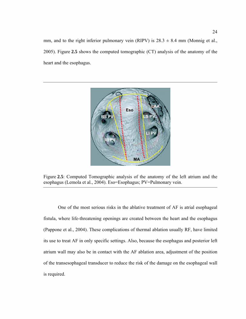
mm, and to the right inferior pulmonary vein (RIPV) is 28.3 ± 8.4 mm (Monnig et al.,
2005). Figure 2.5 shows the computed tomographic (CT) analysis of the anatomy of the
heart and the esophagus.
Figure 2.5: Computed Tomographic analysis of the anatomy of the left atrium and the esophagus (Lemola et al., 2004). Eso=Esophagus; PV=Pulmonary vein.
One of the most serious risks in the ablative treatment of AF is atrial esophageal
fistula, where life-threatening openings are created between the heart and the esophagus
(Pappone et al., 2004). These complications of thermal ablation usually RF, have limited
its use to treat AF in only specific settings. Also, because the esophagus and posterior left
atrium wall may also be in contact with the AF ablation area, adjustment of the position
of the transesophageal transducer to reduce the risk of the damage on the esophageal wall
is required.

25
2.6 Transesophageal devices: An example of transesophageal device in clinical application
The information available on the transesophageal devices currently in clinical use
may be helpful to guide the design and development of the innovative transesophageal
transducer in this thesis. There are several types of transesophageal devices in clinical
application that reduce the need for invasive procedures. Transesophageal
echocardiography (TEE), an advanced configuration of echocardiography, is a non-
invasive diagnostic test. The development of the TEE using ultrasound to produce a
cardiac image was explored in the 1970’s in order to transcend the limits of the
conventional transthoracic echocardiography (Side and Gosling, 1971;Frazin et al.,
1976). Since the esophagus is immediately adjacent to the heart, the TEE delivers a
distinct image of the heart without any interference from the lungs, skin, chest wall or rib
cage. A small transducer with an endoscope is guided through the throat into the
esophagus. The transducer emits ultrasound waves into the heart, and the reflected sound
waves received by the transducer are transformed into an image of the heart.
The purpose of the TEE is to assess the structure and function of the heart
including parameters such as the size of the heart, thickness of the myocardium, its
pumping strength, and the location and extent of any damage to its tissues. It is especially
useful in cases in which conventional transthoracic echocardiography cannot obtain clear
images, such as when the patient has a thick chest wall. The TEE is also used during
cardiac surgery to monitor the effects of surgical intervention to the heart.
The TEE can cause unease to the patient due to gagging. The transducer in a tube
about the diameter of 0.95 to 1.25 cm and 1.2 m long is inserted into the esophagus by

26
swallowing when placed in the back of the patient’s throat. Patients may experience the
discomfort of a sore throat for a while but this usually disappears when the transducer is
in the correct position for imaging. The TEE also may have possible risks when the
transducer is passed down into the throat. In rare cases, the procedure may cause bleeding
or perforation of the esophagus or an inflammatory condition.
Other applications include the transesophageal endoscopic therapies and the
transesophageal electrical cardioversion (TEC). The transesophageal endoscopic therapy
is used to reduce the digestive capacity by lessening the small intestine. The TEC is a
method for the treatment of the atrial fibrillation (AF), in which a low electric current
through an esophageal catheter is used to reset the heart’s abnormal rhythm back to its
normal rhythm.

Chapter 3
Ultrasound for thermal treatment
3.1 Fundamentals of therapeutic ultrasound
3.1.1 Description, brief history, and applications of ultrasound in clinical field
Acoustics was originally defined as the study of slight pressure fluctuation in air,
which can be perceived by the human ear (sound.) The scope of acoustics has been
extended to higher (ultrasound, > 20 kHz) and lower (infrasound, < 20 Hz) frequencies,
as well as to the media other than air, in which the acoustic waves propagate - such as
solids, water, and the human body. In the research relevant to this thesis, acoustic waves
are limited to ultrasound with high intensity, which propagates through and interacts with
human/animal tissue or liquid such as water and blood. Ultrasound interacts differently
with different kinds of tissue or matter. The interactions primarily depend on the acoustic
properties of the tissue, including attenuation, absorption, impedance and sound velocity.
Ultrasound technology has rapidly evolved since the phenomenon of
piezoelectricity in certain crystals was discovered by Pierre Curie and his brother Jacques
Curie (Curie and Curie, 1880). The piezoelectric effect is the physical phenomenon that a
piezoelectric crystal, such as quartz, develops an electric charge upon the application of
stress or a change in dimension when placed in an alternating electric field. These
materials began to be used as high frequency oscillators, and for producing ultrasound

28
generators. Following the development of the piezoelectric transducer, ultrasound waves
were used by the military for SONAR applications during World War II. Some of the
principles developed at that time have led to the clinical imaging applications of
ultrasound. The first clinical use of ultrasound was an investigation of brain tumors
reported by an Austrian psychiatrist (Dussik, 1942). Later, the development of practical
technology and applications has been successfully achieved by Professor Ian Donald and
his colleagues in Glasgow. In their work, the use of an ultrasound transducer to
distinguish cystic and solid masses in the abdomen was demonstrated, and this was a
major milestone in biomedical practice of the ultrasound (Donald et al., 1958).
Research in biomedical ultrasound has persistently investigated the potential use
of ultrasound technology in the field of clinical diagnosis as well as therapy. In the
medical area, these uses include the noninvasive examination of the body for diagnosis as
well as regional heating of parts of the body, the selective destruction of tissue, and the
delivery of drugs for therapy. Recently in the field of thermal therapies and ablation,
biomedical ultrasound has expanded its applications to include heating for muscle pain or
bone break healing, cancer treatment, and brain lesion treatment. Furthermore using
noninvasive ultrasound technology with a combination of specialized ultrasound
generation using focused arrays, signal processing, and visualization of the data (e.g.
Magnetic Resonance (MR) -guided), it is possible to provide more accurate treatment and
real time feedback and control.

29
3.1.2 Applications of therapeutic ultrasound
A therapeutic ultrasound system uses ultrasound to increase the temperature in a
targeted area or to enhance skin permeability for therapeutic purposes. Currently
physiotherapy, hyperthermia, cancer treatment using thermal ablation, and transdermal
drug delivery are typical applications either investigated or commercially developed in
the field of the therapeutic ultrasound. Ultrasound can achieve those by means of
attenuation and absorption of ultrasound waves as well as by the physiological effects of
the microcavitation due to pulsed ultrasound (Holland and Apfel, 1989). There is no
specific frequency of ultrasound waves required for therapy, but previous experiments
suggest that ranges from 0.75 to 3 MHz are appropriate for the effective treatment of
hyperthermia for physiotherapy (Szabo, 2004), 0.5 to 10 MHz for thermal ablation (ter
Haar, 1995), and 1 to 3 MHz for drug delivery (Mitragotri et al., 1995), respectively.
These are relatively low compared to the frequency range for diagnostic ultrasound
imaging, from 1 to 50 MHz (higher frequencies for intravascular imaging).
Therapeutic ultrasound is one of the most effective rehabilitative treatments for
soft tissue injuries (Nussbaum, 1997). Frequently, therapeutic ultrasound treatment is
prescribed as a means to improve healing of soft tissue injuries, as well as to offer pain
relief linked with such injuries. The treatment is achieved through generation of
excessive heat around injured tendons or muscle, which causes the molecules to collide,
resulting in a deep heating effect. The thermal effects of ultrasound promote healing by
increasing metabolism and blood flow and allowing more nutrients and oxygen to reach
the injured tissues while decreasing pain of the damaged area (Nybo et al., 2002).

30
Currently many commercial systems for diathermy are approved for clinical use to treat
usually deeper tissue injuries (~ 4 cm) in physiotherapy.
Thermal ablation using ultrasound for cancer treatment is a relatively recent
technology, which is the therapeutic application of heat (temperatures above 50°C) to
destroy cancerous tissue (Zimmer et al., 1995). Local hyperthermia in the tissue induces
protein destruction and cell membrane dissolution to necrose the targeted tissue. There
are two main types of applications of ultrasound in which hyperthermia can be used. One
is an external application of high-energy waves that are aimed at a tumor near the body
surface from an applicator outside the body. Another type uses a thin probe that is
inserted directly into the tumor. The transducer of the probe delivers ultrasound energy,
which raises the temperature of the surrounding tissue. As an example of intracavitary
application of ultrasound thermal ablation, Figure 3.1 shows a commercial system
(SONOBLATE 500®, Focus Surgery Inc., Indianapolis, Indiana), used to treat the benign
prostatic hyperplasia (BPH). This system consists of a console, chiller, display, and
transrectal ultrasound applicator that combines a therapy probe with an ultrasound
imaging probe. Two focal length transducers of 3.0 cm and 4.0 cm are available for total
prostate ablation (Tan et al., 2001).
Another example of therapeutic ultrasound applications is ultrasound-mediated
noninvasive transdermal drug delivery. For more than a decade, transdermal drug
delivery has been explored as an alternative method of painless drug administration.
However, there was a restriction that high molecular weight proteins such as insulin
could not be delivered through the skin due to the very low permeability of human skin
(Scheuplein and Blank, 1971). The ultrasound-mediated method is an innovative

31
technology to overcome this drawback. Using ultrasound at low frequencies (< 3 MHz),
the method can improve the penetration of large molecular weight substances through the
skin (Mitragotri et al., 1995). Even though the mechanisms are not yet fully understood,
the theory that acoustic cavitation combined with a thermal effect induced from
ultrasound energy can enhance skin permeability is an accepted concept (Smith et al.,
2003a). Currently there is no commercial product for transdermal drug delivery using
ultrasound approved for clinical use. In vivo transdermal delivery of insulin with low-
profile cymbal ultrasound arrays has been reported (Smith et al., 2003b).
Figure 3.1: A picture of Sonoblate 500® thermal ablation system (Focus Surgery Inc., Indianapolis, IN).

32
3.1.3 Focused ultrasound surgery (FUS)
High Intensity Focused Ultrasound (HIFU) or Focused Ultrasound Surgery (FUS)
is an emerging ablation technique for localized cancer therapy or an alternative surgical
method using acoustic energy. FUS uses intersecting acoustic waves on a single location
to increase temperature and to selectively destroy the target tissue. Due to its non-
invasive nature, FUS has been explored as an alternative energy source for new surgical
methods.
3.1.3.1 Mechanism of ultrasound surgery
The majority of energy sources create lesions via hyperthermic injury. In the case
of atrial injury, the goal of hyperthermic ablation is to obtain a tissue temperature of
50°C, the temperature at which electrophysiologic disruption occurs (Nath et al., 1993). It
is important that the tissue temperature does not exceed the boiling point of water
(100°C) in order to avoid cavitation and/or tissue disruption. The cellular mechanism for
hyperthermic ablation is not entirely understood but is likely to be related to injury of the
sarcoplasmic reticulum with resulting influx of calcium into the cytosol (Williams et al.,
2004).
In thermal ablation, the ultrasound with high-intensity is focused on a targeted
area to produce irreversible tissue necrosis (ter Haar, 1995). Significant lesions are
typically achieved at exposure of 5 to 15 seconds, and high temperatures of up to 60 to
100°C (Chen et al., 1997). Induction of hyperthermia in tissue above 50°C causes the
protein to be permanently destroyed and cell membranes to be dissolved.

33
3.1.3.2 Clinical applications
The first commercially available HIFU system was the Ablatherm® (EDAP, Lyon,
France). This is a device used in prostate cancer treatment. A HIFU probe with a single
focal length of 40 mm is placed into the rectum after administration of spinal anesthesia.
The temperature inside the prostate is raised to 85°C using a focused ultrasound beam. It
is approved in the EU, Canada, Russia and South Korea, but it is not available yet in the
US where a clinical trial is ongoing.
Subsequently, a second-generation system called the Sonablate 500® for non-
invasive prostate cancer therapy was developed by Focus Surgery (Indianapolis, IN). It
has a combined therapy and imaging transducer for an image-guided ultrasound ablation
and is available for multiple focal lengths to increase the resolution of the treatment plan.
Comparison between the results of both systems has been encouraging and the progress is
in development for HIFU systems as well as their clinical applications.
3.2 Ultrasound transducer array
This section discusses topics concerning modern ultrasound transducers in arrays
for either imaging or therapy. Generally there are three different types of multi-element
transducer arrays, which are linear, curved linear, and phased arrays as shown in
Figure 3.2 to Figure 3.4 (Jensen, 1999). Each type is suited to a different application and
each produces a different beam shape. Although array models presented in this section
are applications for imaging transducers, this information may also be helpful to
understand therapeutic ultrasound arrays.

34
3.2.1 Types of array
3.2.1.1 Linear Array
Linear phased array analysis often assumes that the array elements are equally
spaced, and identical, which provide the simplifications that facilitate analytical solutions
to synthesis problems. A typical linear array ultrasound transducer is composed of a large
number of rectangular piezoelectric material elements. The beam radiated from a single
element will diverge quickly after it is emitted. The array overcomes this to result in
better resolution and higher sensitivity. This type of array is widely used in ultrasound
imaging devices. Linear arrays for imaging obtain and display a rectangular image, and
the maximum region of interest (ROI) will be the same as the lateral size of the whole
transducer array. Figure 3.2 depicts a linear array transducer generally used for imaging
transducers.
Figure 3.2: Sketch of linear array transducer (Jensen, 1999).

35
With a linear phased array, an imaging line is formed by using a group of
elements, which emit and receive ultrasound monostatically. The ROI moves laterally by
firing sets of adjacent elements (Oakley, 1994;Jensen, 1999).
3.2.1.2 Curved Linear Array
Because curved linear array has a convex shape, it fits better in the body and
radiates the ultrasonic beam toward a wider field than a linear array transducer having the
same lateral extent. The beam region widens with distance from the array with angles
varying from 30° to over 90°. The method of beam-forming and focusing is the same as
that of the linear array. Figure 3.3 depicts a curved linear array transducer generally used
for imaging transducers.
Figure 3.3: Sketch of curved linear array transducer (Jensen, 1999).

36
3.2.1.3 Phased Array
Because linear arrays and curved linear arrays are often too large for some cases
such as cardiac imaging during which beams pass through the ribs, a phased array is
appropriate for obtaining a large field of view with a small array size. All the array
elements are pulsed to form a beam for either imaging or therapeutic treatment, and each
beam has its own steering angle with respect to the transducer surface. The method of
element combination is the same for linear and curved linear arrays. The direction of the
beam, however, is steered by phasing or delaying individual elements. For focused
ultrasound ablation, a two-dimensional phased array has been generally used. By the
control of the phase and amplitude of the sound wave generated from each element of the
array, beams can be focused electronically at different depths and steered or shifted
automatically. Figure 3.4 shows a linear phased array transducer generally used for
imaging.
Figure 3.4: Sketch of phased array transducer (Jensen, 1999).

37
3.2.2 Focusing
In order to either improve imaging quality for diagnostic ultrasound transducers
or to localize acoustic energy at an aimed point for the therapeutic ultrasound transducer,
focusing is commonly used. Focusing in the plane along the line of the aperture improves
the resolution as well as the sensitivity by increasing the amount of energy in the focal
area (Zagzebski, 1996). The acoustic pressures and intensities involved are much higher,
when the focal rezone is well defined. Focusing can be achieved by an electric delay
scheme, or using an acoustic lens at the face of the transducer as shown in Figure 3.5.
Focal point
Figure 3.5: Ultrasound beam foacoustic lens.
(a) Electric focusing (a) Electronic focusing
Focal point
Geo. center
s
(b) Acoustic len(b) Acoustic lenscusing technique by (a) electronic focusing and (b) an

38
Electronic focusing is applied to individual ultrasound beams generated by a
group of elements. Focusing during transmission, as shown in Figure 3.5 (a), is obtained
by adding delays to the excitation pulse of each element in a group. A concave shaped
beam from the aperture is transmitted and focused at the focal point, which is determined
by the extent of delay. The time-delay (ti [s]) scheme within a beam depends on the
position of the focal point and can be expressed as:
( ) ( ) ( )2221fififii zzyyxx
ct −+−+−= (3.1)
where c is the speed of sound [m/s], ( )iii zyx ,, is the center for the physical elements i
[m], and ( )fff zyx ,, is the position of the focal point [m] (Jensen, 1999). The depth of
the focal point for electronic focusing can be changed simply by changing the amount of
delay applied to the individual element.
Elevation focusing using an acoustic lens, as shown in Figure 3.5 (b), is also
achieved by ensuring the contributions of the pressure field from all elements of the
aperture arrive at the field point at the same time. The amount of continuous phase delay,
nφ [rad], along the elevation direction of the element depends on the thickness of the lens
and can be expressed as:
( )lens
lensn
ndλ
πφ
2= (3.2)
where is the thickness of the lens at the elevation position divided by the number
of rays [m], and
( )ndlens
lensλ is the wavelength within the lens material [m]. The total ultrasound

39
field (p [Pa]) is calculated by summing up the Green’s function of each sound field from
a simple virtual source of the elevation position with a corresponding phase delay as
( )
∑=
+
=N
n n
kRj
Rep
nn
1
φ
(3.3)
where k is the wave number [m-1], is the distance between the field point and the
position of a simple virtual source [m]. An acoustic lens has the major disadvantage that
the focal point cannot be adjusted.
nR
3.2.3 Sparse array
To have full electronic control for focusing and steering, the distance between two
adjacent elements (pitch) should be half of the wavelength of the ultrasound in the
propagation medium (λ/2-pitch requirement). For instance, an array with a square
aperture that has a length of 11 mm at a frequency of 3.5 MHz will need of 50-by-
50=2500 elements with a pitch of 220 µm. Each of these elements should be connected to
a channel of the ultrasound driving system. Using existing technologies, the fabrication
and implementation of arrays with that large a number of elements is very difficult and
expensive. One possibility to reduce the number of channels is the use of sparse array
techniques (Lo, 1964;Goss et al., 1996;Holm et al., 1997). The fully sampled or dense
array, as it is called when containing all elements, is thinned by randomly removing
elements until a given order of reduction is reached. Past research has shown that the
main lobe of the radiation pattern is mostly unaffected by random removal but the

40
average sidelobe level increases as the number of channels decreases (Turnbull and
Foster, 1991).
A sparse phased array has been modeled and constructed for focused ultrasound
surgery (Goss et al., 1996). This array consists of a hexagonally packed transducers
composed of 108 elements. All the elements, mounted on a spherical shell, were identical
in shape and size, with a circular shape and 8 mm diameter. This design used a subset of
64 elements driven at 2.1 MHz, which were randomly sampled from the overall 108 array
elements. The array has demonstrated that the sparse random array reduced the
periodicity of the elements and thus the grating lobe level. The results of this study have
highlighted the feasibility of using sparse random arrays for focal surgery. A sketch of
this array is shown in Figure 3.6.
Figure 3.6: A sketch of a sparse random array for focused ultrasound surgery (Goss et al., 1996)

41
The grating lobe problem of a sparse array can be viewed as a problem of
reconstructing a continuous signal from discrete samples. Roughly, the sampling density
of the sparse array is not sufficient to reconstruct the signal without aliasing.
3.3 Thermal distribution on tissue
3.3.1 Bio-heat transfer model of tissue
The prediction of heat distribution in the targeted area is crucial in deciding the
input power and the required sonication time for thermal ablations. Many heat transfer
models for tissues have been described to date. Pennes (1998) was the first to develop a
heat transfer model for perfusion. His model was simple and considered the effect of
perfusion as a source-sink relationship between the vessels and the tissue. The model was
characterized by the following equation often referred to as “the Bio-Heat Transfer
Equation (BHTE)”:
( ) qTTwCTtTC abt +−+∇⋅∇=∂∂ κρ (3.4)
where ρ is the density of the tissue [kg·m-3], Ct is the specific heat of the tissue [J·kg-1·°C-
1], T is the temperature at time t at the point x, y, z in °C, κ is the thermal conductivity
[W·m-1·°C-1], Cb is the specific heat of the blood [J·kg-1·°C-1], w is the blood perfusion
rate in tissue [kg·m-3·s-1], Ta is the arterial blood temperature [°C], and q is the power
deposited at the point x, y, z in Watts.
In Equation 3.4, the first term on the right-hand side is the heat diffusion due to
conduction. The second term is the heat transfer due to the perfusion of blood. The blood

42
perfusion rate in tissue models the effect of blood flow on the temperature distribution in
the tissue. The main assumption behind the model was that the vessel temperature was
constant and the heat transfer took place predominantly in the capillaries. The model
assumes that the arterial blood enters the capillary bed at a certain temperature (Ta) and
then instantaneously equilibrates with the tissue temperature, leaving the tissue at the
temperature, T. In this study, the metabolic heat generation term is ignored due to its
small effect on the temperature distribution. The last term on the right-hand side is the
heat generated in the tissue due to the power deposition from the focused ultrasound
energy expressed as
( ) ( )c
zyxPIzyxq net
ρα
α,,
2,,2
== (3.5)
where, α is the attenuation coefficient in the medium [dB·cm-1·MHz-1], and Pnet is the net
sound pressure at a given point in Pa. Figure 3.7 shows some attenuation coefficients for
mammalian tendon, heart, and liver.

43
Figure 3.7: Graph of the attenuation coefficient versus frequency (0.5-7 MHz) for mammalian tendon, heart and liver. (Goss et al., 1979)
3.3.2 Thermal dose
It was found that a mass of cancer cells is destroyed when the temperature is
raised to 113°F (45°C) and maintained for ten minutes (Percy, 1916). This discovery has
drawn attention to the beneficial effects of thermal therapy upon cancerous growths.
Recent in vitro studies of the effects of heat on Chinese hamster ovary cells has revealed
that the shape of survival curves appear similar to those representing cell survival as a
function of a dose of ionizing radiation (Dewey et al., 1977). This information indicates
that mechanisms for killing cells are different for heat treatment below 43°C as compared
to above 43°C. To compare the heat accumulation “dose” by different tissues subject to a

44
complex heating regime, an equivalent time (teq) is calculated to have the same biological
effect if the temperature has been held at 43°C (Sapareto and Dewey, 1984). Thirty
minutes of constant thermal exposure at 43°C (t43) has been found to be sufficient to
cause the required biological effect for hyperthermia treatments.
The most commonly used model for describing tissue damage mathematically is
the Arrhenius model (Sapareto and Dewey, 1984). It has been shown for many tissue
types, that there is an exponential relationship between necessary treatment time and
temperature to cause tissue damage. In most cases, the following law applies above 43°C:
with every increase in tissue temperature by one °C, treatment time to cause tissue
damage is cut in half. The relationship stated above can be mathematically described by
the isoeffect equation:
( )2121
TTRtt −⋅= (3.6)
where t1 and t2 are the treatment durations at treatment temperatures T1 and T2,
respectively. R can be assumed a constant with a value of 0.5 above 43°C, and 0.25
below 43°C (Sapareto and Dewey, 1984). Because the onset of appreciable tissue damage
occurs at around 43°C, it has been suggested by Sapareto and Dewey (1984) to quantify
tissue damage by a thermal dose at 43°C. This thermal dose is expressed as cumulative
equivalent minutes at 43°C (CEM43); i.e. a certain thermal treatment has the same effect
as keeping the tissue at 43°C for CEM43 minutes. If we set T1 = 43°C in the (1) and
allow the temperature to be changed during the treatment, we obtain:
( )( )∫ −= dtRCEM tT4343 (3.7)

45
Once CEM43 exceeds a certain critical value we can consider the tissue to be
damaged (i.e. ablated). The critical value of CEM43 has been measured for many tissues,
and is around 340 min for liver (Graham et al., 1999); i.e. tissue with CEM43 > 340 min
we considered ablated.

Chapter 4
Array design and numerical analysis
This chapter presents the numerical simulations used for acoustic pressure field
calculations, the design of the ultrasound phased array, and thermal distribution within
the cardiac tissue model, as well as a discussion of the underlying assumptions and some
background information. Efforts were made to model both single element and transducer
arrays by integral equation formulations using MATLAB® (MathWorks, Inc., Natick,
MA). The far field properties of the transducer element and arrays were then calculated.
Lastly thermal distribution generated by the ultrasound energy within the myocardium
(atrial wall) and the thermal dose required for tissue ablation were simulated with a finite
difference scheme in MATLAB® v7.0. The numerical methods, the procedures for
analysis using the commercial programs and the overall findings will be discussed.
4.1 Acoustic pressure calculations
Acoustic pressure calculations are required to determine the size and the number
of array elements in addition to predicting the ultrasound beam fields and temperature
distribution produced from the applicator. For the calculation of pressure fields from the
transducer array, an ultrasound beam model for a rectangular transducer has to be defined
since each element of the ultrasound array used in the current research has a rectangular
shape. In this study, two numerical models, one based on the Rayleigh-Sommerfeld

47
integral and the other based on the Tupholme-Stepanishen method, are used for the
calculation of the ultrasound beam field radiating from a baffled rectangular piston
transducer as well as from a phased transducer array. The fundamental idea of these
approaches is that pressure field radiating from the transducer can be calculated by
summing up the resultant fields from small segments over the transducer face. All the
calculations follow the rigid-baffle assumption. The results from each model are
compared to verify the validity of the numerical method for the pressure calculations.
4.1.1 Rayleigh-Sommerfeld integral
The Rayleigh-Sommerfeld integral gives the pressure field produced in a medium
at x from a planar piston source (Zemanek, 1971):
( ) ( )dSr
jkrUjxp
S∫−
=exp
2, 0
πωρ
ωr , (4.1)
where ω is the angular frequency [rad], ρ is the density of the medium [kg·m-3], U0 is the
particle speed on the aperture surface e[m/s], r is the distance from a point on the aperture
surface to field point [m] and S is total transducer surface area in mxr 2.
Based on the single element beam model, the focused ultrasound field radiating
from the phased array will be predicted by superposition of the pressure field of each
element with appropriate phase delays of the driving signals. The phase of ith element, iφ
[rad] is given by:
( )02 ddii −=λπφ , (4.2)

48
where λ is the wavelength in the interrogated medium [m], di is the distance from the
center of ith element to the focal point [m], and d0 is the distance from the center of the
array to the focal point [m]. Therefore, the total acoustic pressure at any field point, xr ,
produced by an array with n number of elements can be written as:
( ) ( )[ ]∑ ∫=
−−=
n
iiS
i
ii dSrkrjUj
xpi1
0 exp2
,φ
πωρ
ωr . (4.3)
The Rayleigh-Sommerfeld approach has been used fairly extensively to treat the
problem of ultrasound transducer designs due to its simplicity. It can calculate ultrasound
beam patterns propagated through a planar interface from the linear phased array.
However, because Rayleigh-Sommerfeld method requires long calculation times, a more
efficient numerical method for beam models is desired.
4.1.2 Tupholme-Stepanishen method
Because of its simple expression, the spatial impulse response method is
frequently utilized to calculate the pressure field generated from pistons in an infinite
rigid baffle, radiating into a homogeneous medium (Wu and Stepinski, 1999). The
method counts on a linear systems theory to find the ultrasound field. One such approach
was developed by Tupholme (1969) and Stepanishen (1971). The calculation for the
ultrasound beam field radiating from the aperture can be achieved in a simple form using
the spatial impulse response:
( ) ( ) ( )trht
tutrp n ,, 11
rr∗
∂∂
= ρ , (4.4)

49
where * denotes the time convolution, is the normal velocity to the aperture surface
[m·s
nu
-1], and denotes the field point. Here, spatial impulse response, relates
aperture geometry to the spatial extent of the field and depends on the difference between
and :
1rr ( trh ,1
r )
1rr
2rr
( ) ∫ −
⎟⎟⎠
⎞⎜⎜⎝
⎛ −−
=S
dSrr
crr
ttrh
21
21
1 2, rr
rr
r
π
δ,
(4.5)
where denotes the aperture. In order to find the spatial impulse response, one can
consider the geometrical information between the field point and the aperture, as well as,
the shape of the aperture. Mathematical manipulations give the simplified general
expression for the spatial impulse response as:
2rr
( ) ( ) ( )[ ]( )
∑=
Θ−Θ=tN
ittctrh
1121 2
,π
r , (4.6)
where N(t) denotes the number of arc segments that are intersected by the projected
spherical wave onto the aperture, and ( ) ( )[ ]tt 12 Θ−Θ is the corresponding angle
differences of the arc [rad].
If the spatial impulse response is found, the sound pressure field can be simply
identified using the geometrical information of the transducers as shown in Equation 4.4.
The spatial impulse response method devised by the Tupholme-Stepanishen can calculate
the ultrasound pressure field with a particular geometry of the aperture. More detail of the
Tupholme-Stepanishen method is given in Appendix A.

50
4.1.3 Calculation of radiation beam fields
For calculations of pressure fields, simulation programs using the Rayleigh-
Sommerfeld integral (Equation 4.1) were written with MATLAB® while programs using
the Tupholme-Stepanishen approach (Equation 4.4) were implemented using the FIELD
II programs that are MATLAB® functions developed for calculating ultrasound fields
(Jensen, 1996). The results from the calculation of radiation beam fields from a single
rectangular transducer and a linear phased array using the two numerical models are
presented and compared to each other for the validation of the developed programs. The
MATLAB® program code can be found in Appendix B.
4.1.3.1 Single rectangular transducer
Using the numerical approaches introduced in the previous sections, the pressure
fields in water (speed of sound: 1500 m/s) from a planar square element (5 × 5 mm) were
simulated. Figure 4.1 describes the definition of the coordinate axes and a plane
rectangular piston for sound pressure calculations. In this coordinate system, the element
is divided into 900 rectangular sub-elements required for superposition calculations. As
shown in Figure 4.2 and Figure 4.3, predictions using the two approaches of both on-axis
(axial response) and off-axis (lateral response) pressure fields in addition to the xz-plane
pressure fields agree very well. Lateral responses (Figure 4.2, 4.3 (a)) were calculated at
the field point, z = 10 mm, close to the axial distances of the near-field/far-field transition
distance, z ≈ 7 mm (d2 / 4λ, where d is the length of a side of the element.) Axial
responses and the near-field/far-field transition distance are shown in Figure 4.2, 4.3 (b).

51
When the speed of transducer surface is assumed to be U0 = 0.019 m/s at 1.6 MHz, the
calculated values at the maximum pressure field were 5.0840×10⁴ Pa (Figure 4.2 (c))
using the Tupholme-Stepanishen method and 5.1046×10⁴ Pa (Figure 4.3 (c)) using the
Rayleigh-Sommerfeld integral, respectively. Figure 4.2, 4.3 (d) show the normalized
sound intensity maps as indicated from the intensity color bar. Also, Figure 4.4 shows the
angular responses that represent the far field properties of the transducer element. As
expected, the results of the simulated pressure fields show close agreement between the
two calculation models. Thus, either the Rayleigh-Sommerfeld integral or the Tupholme-
Stepanishen method can be adopted for a rectangular transducer.
x
y
z
(x0, y0, z0)
width
height
sub-element
Figure 4.1: Definition of the coordinate axes and a plane rectangular piston for sound pressure calculations. The center of the element defines the origin of the coordinate system and the pressure is calculated at field point, (x0, y0, z0). The z-axis is coincident with the element normal.

52
(a) Lateral response of the transducer (b) Axial response of the transducer
at z = 10 mm
(c) Sound pressure field on axis plane (d) Normalized sound intensity map
at y = 0 mm
Figure 4.2: Numerical results of the ultrasound pressure field of a planar rectangular transducer with 5 × 5 mm2 in size at 1.6 MHz using the Tupholme-Stepanishen method.
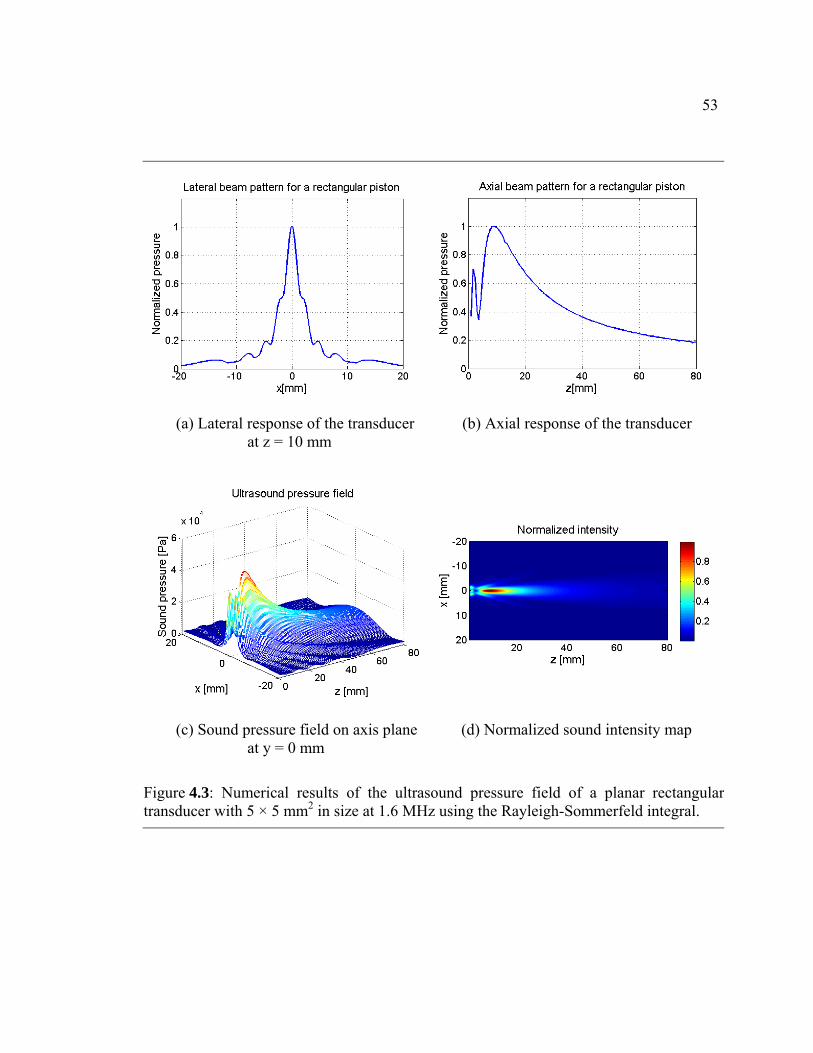
53
(a) Lateral response of the transducer (b) Axial response of the transducer
at z = 10 mm
(c) Sound pressure field on axis plane (d) Normalized sound intensity map
at y = 0 mm
Figure 4.3: Numerical results of the ultrasound pressure field of a planar rectangular transducer with 5 × 5 mm2 in size at 1.6 MHz using the Rayleigh-Sommerfeld integral.

54
Figure 4.4: Numerical results of the angular response at the far-field of a planar rectangular transducer with 5 × 5 mm2 in size at 1.6 MHz.
Rayleigh-Sommerfeld integral Tupholme-Stepanishen method
For validation of the algorithms for the linear phased arrays, the following section
will demonstrate the simulation of the angular response and the sound pressure field
generated from a multi-element transducer.
4.1.3.2 Multi-element transducer
The methods used for single elements in the previous section were adapted and
modified to calculate the acoustic field in a lossless medium for a multi-element
transducer. The pressure fields in water were simulated from a 1-D linear phased array
composed of 32 elements with a pitch equal to the wavelength and with an element width
equal to 0.9 times the wavelength. Electrical focusing on axis at (0, 0, 40) mm and beam

55
steering to the off-axis focal points of (20, 0, 40) mm are applied with appropriate phase
delays of the driving signals to each element. The sound intensities were calculated for
longitudinal sections in the y = 0 plane (zx-plane) with the values normalized. The results
are shown in Figure 4.5 using contour plots of dB levels, as indicated from the intensity
color bar. The results from both the numerical models for the pressure field appear in
close agreement for either on-axis focusing or off-axis focusing. In Figure 4.5 (c) and (d),
though the patterns of grating lobes induced from steering with arrays show slight
differences, the main beam patterns reveal the focusing for thermal ablations. Finally,
radiation patterns with the two numerical models were calculated and compared with an
analytical solution using the product theorem given as ( ) ( ) ( ) ( )φθφθφθ ,,,, HHrPrP eax= ,
where H is the directional factor for the array with simple sources at the position of each
element and He is the directional factor for a single element (Kinsler et al., 2000).
Figure 4.6 shows that the results of the calculation using the Rayleigh-
Sommerfeld integral agree well with available analytical results. However, the results
from the Tupholme-Stepanishen method do not agree in the levels of grating lobes. As
shown in results of off-axis focusing, large grating lobes at θ =50° occur with a beam
steering toward θ =14° even thought there were no grating lobes in the non-steered beam
fields. Because grating lobes are a source of unwanted heating in tissue, these must be
carefully considered for the array designs.

56
(a) Focusing at (0, 0, 40) mm (b) Focusing at (0, 0, 40) mm
using the Rayleigh-Sommerfeld integral using the Tupholme-Stepanishen method
(c) Focusing at (20, 0, 40) mm (d) Focusing at (20, 0, 40) mm
using the Rayleigh-Sommerfeld integral using the Tupholme-Stepanishen method
Figure 4.5: Numerical results of a normalized sound intensity map of a linear focused phased array with 32-elements and a wavelength in pitch size at 1.6 MHz using the Rayleigh-Sommerfeld integral ((a) and (c)) and the Tupholme-Stepanishen method ((b) and (d)). (a) and (b) show contours of on-axis focusing at (0, 0, 40) mm and (c) and (d) shows off-axis focusing at (20, 0, 40) mm.
Grating lobe Grating lobe

57
(a) and (b) used the Rayleigh-Sommerfeld integral
(c) and (d) used the Tupholme-Stepanishen method
(e) and (f) used the analytical solution
Figure 4.6: Numerical and analytical results of the sound radiation pattern at far-field from a linear non-focused phased array with 32-elements and a wavelength in pitch size. (a), (c), and (e) are non-steered. (b), (d), and (f) are steered toward θ =14°.
Grating lobe
Grating lobe
Grating lobe

58
Preliminary simulations with both the single planar rectangular transducer and a
linear phased array transducer verified the validity of the numerical models as well as
demonstrated the predicted acoustic behavior. The programs developed for the ultrasound
field with a linear phased array are available for proper prediction of the sound pressure
at a certain area. The pressure fields for this study were calculated for the array designs
based on these numerical models. The Rayleigh-Sommerfeld integral required more
calculation time than the Tupholme-Stepanishen method for the identical transducer
model. However, because the FIELD II program, which uses the Tupholme-Stepanishen
method, cannot model a random sparse array, and the Tupholme-Stepanishen method
dose not agree as well with analytical solutions, the Rayleigh-Sommerfeld integral was
used as the main numerical model for the calculations of the pressure fields in this study.
4.2 Ultrasound transducer array design and simulations
The esophagus is close to the posterior of the left atrium. This position makes it
particularly attractive for the incision-less surgery of selected areas of the heart. For the
focused ultrasound ablation through the esophagus, a transducer design based on details
of human anatomy and physiology is required. Ultrasound pressure fields within tissues
are numerically simulated to evaluate the designs of ultrasound arrays. With the
transesophageal applicator, the size and the position of the ablation targets can be
controlled by changing the electrical power and phase to the individual elements for
ultrasound beam focusing and steering. For the verification of the suggested design, the

59
phased array with an acoustic impedance matching layer was built (Chapter 5), and then
evaluated using exposimetry and ex vivo experiments (Chapter 6).
4.2.1 Array designs
4.2.1.1 Overview
The basic principles of transducer array design for the therapeutic ultrasound
applicator are described from both theoretical and practical perspectives. For focused
ultrasound ablation, the transducer design is a two-dimensional phased array operating at
a frequency between 1~2 MHz. Phased arrays use multiple small transducer elements to
produce a focal area that is capable of heating a large volume of tissue in a single
exposure. By the control of the phase and amplitude of the sound wave generated from
each element of the array, beams can be focused electronically at different depths and
steered or shifted automatically. Also, the axial/lateral resolution and the beam pattern
can be changed through adjustment of the scheme of the active aperture. Since focused
ultrasound transducer arrays rely on array layouts to deliver maximum power to the focal
area, a careful choice of array design is essential.
The ultimate design goal of the current research is that the ultrasound applicator is
located within the esophagus as close as possible to the heart in order to effectively
deliver ultrasound energy, and create electrically isolating lesions in myocardial tissue
replicating the Maze procedure. A transesophageal ultrasound applicator must be small to
allow insertion into the esophagus. It must avoid possible damage to the esophagus while

60
being inserted. According to a clinical study, the mean diameter of the esophagus is 18.6
± 1.6 mm (range 15.4-22.0) (Tsao et al., 2006). Also, the applicator must be able to
generate sufficient high sound intensity and have the capability of beam steering.
For the design of the transesophageal ultrasound transducer, various layouts of
transducer arrays and the corresponding ultrasound pressure fields were modeled. The
total acoustic intensity at any point in the sound field was calculated using the
MATLAB® implementation of the Rayleigh-Sommerfeld equation. The aperture size for
array design was 20.70 × 10.24 mm2, which is based on the dimensions of the human
esophagus as well as the housing of the array. Two types of sparse phased array design
have been examined in this dissertation and one of them was constructed using
piezoelectric ceramic (PZT-8) elements. Because of the small array element sizes, and
subsequent low capacitance and high impedances, a ceramic with a very high relative
dielectric constant and high coupling factor was considered.
4.2.1.2 Array profile with radiation pattern
For evaluation of the simulations of the phased ultrasound array, grating lobes and
f-number of the beam shaping are important output parameters. Grating lobes are the
additional beams resulting from multi-element structures. In this study, the magnitude of
the first grating lobe is observed as an output parameter for array design. Because grating
lobes might induce thermal damage on normal tissue outside the targeted area, these
unwanted beams must be minimized during the array design. Angles of grating lobes can
be calculated with

61
,...3,2,1sin == nd
ng
λθ (4.7)
where d is the distance between the center of elements. If λ is larger than d, there are no
grating lobes (Jensen, 1999).
Another important output parameter is f-number, which is defined as the ratio of
focal length to the total aperture size, given as
f-number = f / D (4.8)
where f is the focal length of the phased array [m] and D is the aperture size of the total
array [m]. Although it is known that the smaller f-numbers provide better axial resolution,
the simulation results showed that better lateral resolution as well as better controllability
of focusing and steering were achieved with the smaller f-numbers. Thus, when the
targeted focal length is given, larger apertures allow better performance in beam focusing.
However, there are limitations that prevent transducer arrays from using smaller f-
numbers in order to achieve improvements in beam forming. The channel count limit on
f-number is straightforward. In order to design arrays with larger apertures, more
elements or larger elements are required.
4.2.2 Periodic sparse phased array
Linear phased arrays have been intensively studied for many years. Conventional
analytical and numerical methods of linear phased array synthesis are well developed and
documented in many textbooks and papers. The phased array has been widely used in
medical ultrasound applications since its beams can be focused at different depths and

62
steered by the control of electric signals into each element of the array. Also, the linear
phased array with identically spaced elements is easier to analyze and forms the basis for
most array designs. However, a linear phased array with a compact structure may
produce large grating lobes or low acoustic power delivery due to poor focusing.
Figure 4.7 - Figure 4.9 show the simulation results of the ultrasound field of normalized
intensity using a linear phased array, as indicated from the intensity color bar. Three
different types of designs of the linear phased array, which have different aperture size or
different number of elements, were modeled and the ultrasound fields from the each array
were calculated and compared to each other. The anatomical information of the
esophagus and economical aspect concerning the production of the array were considered
in determining the specifications of the model. The sound fields for on-axis focusing with
the focal point aimed at (0, 0, 40) mm and off-axis focusing at (10, 10, 40) mm were
calculated respectively. First, a simple design (#1) of the array for focused ultrasound
transducer, with an aperture size of 20.70 × 10.24 mm2, 64-elements (8-by-8) in same
size, and kerfs of 105 µm, was modeled (Figure 4.7 (a).) In order to quantitatively
evaluate the focusing, the focal zone is generally defined by the half-maximum intensity
(-3dB) contour. However, it is not necessary for the volume of the focal zone to agree
with lesion size created in targeted tissue, since thermal dose for ablation can be
controlled by the ultrasound exposure time.

63
(a) Design #1 – Aperture size: 20.70 × 10.24 mm2 (8-by-8 array)
(b) Focal point aimed at (0, 0, 40) mm (c) Focal point aimed at (10, 10, 40) mm
Figure 4.7: (a) Scheme of the linear phased array (Design #1) and simulation results ofthe ultrasound field of the normalized intensity for (b) on-axis focusing and (c) off-axis focusing plotted as a contour with levels indicated at 0, -1, -2, -3, -6, -9 and -12 dB,
Grating lobe
The simulation results of on-axis focusing in Figure 4.7 (b) show that the
suggested linear phased array achieved a focal zone length of about 25 mm at the aimed
point (0, 0, 40) mm, and the grating lobe level kept below -9 dB toward θ=22° in the xz-
plane from the main lobe. The results seem to be acceptable for ultrasound ablation of the
myocardium for on-axis focusing. However, since the existence of the grating lobe may
64
possibly result in unwanted heating within the tissue when using long ultrasound
exposure time, this needs to be suppressed with design modifications.
For off-axis focusing (Figure 4.7 (c)), the plot shows that the unwanted focal zone
due to the grating lobe at (-6, 10, 42) mm is greater than that due to the main lobe. The
greater focal zone of the grating lobe can be attributed to the violation of the design
criteria for phased array. Practically, phased array should have a pitch size less than one
half-wavelength in order to avoid raising significant grating lobes, especially when the
beam is steered. Equation 4.7 explains how the pitch size (d) of the array, when the
operating frequency is given, can be chosen to eliminate grating lobes. The array (Design
#1), however, has a pitch of 2.5 mm in the x-direction and 1.2 mm in the y-direction,
which is much larger than the wavelength of 0.94 mm. For this reason, a new design must
have a smaller pitch. In order to see the effect of small pitch size on the beam formation,
a linear phased array with an aperture size of 14.48 × 7.16 mm2 (about 70 % length of
each side of the aperture), 64-elements (8-by-8) in same size, and kerfs of 105 µm, was
modeled as array Design #2 (Figure 4.8 (a).) and the sound fields for on-axis focusing
and off-axis focusing were calculated.

65
(a) Design #2 – Aperture size: 14.48 × 7.16 mm2 (8-by-8 array)
(b) Focal point aimed at (0, 0, 40) mm (c) Focal point aimed at (10, 10, 40) mm
Figure 4.8: (a) Scheme of the linear phased array (Design #2) and simulation results of the ultrasound field of the normalized intensity for (b) on-axis focusing and (c) off-axis focusing plotted as a contour with levels indicated at 0, -1, -2, -3, -6, -9 and -12 dB
Grating lobe
In the case where the array element size was decreased, i.e., the pitch size was
decreased from 2.5 mm (Design #1) to 1.7 mm (Design #2) in the x-direction and from
1.2 mm (Design #1) to 0.8 mm (Design #2) in the y-direction, the ultrasound fields of the
normalized intensity were also calculated and plotted in Figure 4.8. On-axis focusing
with the smaller pitch resulted in an improved grating lobe level below -12 dB toward

66
θ=34° from the main lobe, compared to that from the array of Design #1, which can be
shown in Figure 4.8 (b). Even though the level of the grating lobe was significantly
suppressed, the focal zone length was conversely increased to about 30 mm at the point
(0, 0, 30) mm instead of the aimed point (0, 0, 40) mm. This is caused by high beam
forming f-number at (0, 0, 40) mm, which resulted from the decreased aperture size of the
total array with decreased element size. According to the Equation 4.8, a smaller aperture
size (D) of an array increases the f-number when the targeted focal length is given. This
means that the array with Design #2 cannot control beam formation at the distance of the
focal point (0, 0, 40) mm for a given frequency. From the sound fields simulations with
various f-numbers and from previous studies, the f-number should be kept below two (2)
to ensure that the transducer array generates concentrated focal zones in a tissue volume.
Designs with very small f-number are restricted due to the dimensional limits of the
esophagus.
For off-axis focusing shown in Figure 4.8 (c), an unwanted focal zone, due to the
grating lobe at (-11, 10, 36) mm, also exist in the same manner as in Design #1. There is
still considerable concern about the level and size of the grating lobe. It is imperative that
it is suppressed for the design of ultrasound ablation transducer.
To improve the focusing problem with Design #2, a new design of the linear
phased array with small pitch and large aperture size was suggested by increasing the
number of elements in the aperture size used in Design #1. A linear phased array, which
has an aperture size of 20.70 × 10.24 mm2, 15-by-13 195-elements in same size of 1.3
mm in the x-direction and 0.7 mm in the y-direction, and kerfs of 105 µm, was modeled

67
as array Design #3 (Figure 4.9 (a).) and the sound fields for on-axis focusing and off-axis
focusing were calculated.
(a) Design #3 – Aperture size: 20.70 × 10.24 mm2 (15-by-13 array)
(b) Focal point aimed at (0, 0, 40) mm (c) Focal point aimed at (10, 10, 40) mm
Figure 4.9: (a) Scheme of the linear phased array (Design #3) and simulation results of the ultrasound field of the normalized intensity for (b) on-axis focusing and (c) off-axis focusing plotted as a contour with levels indicated at 0, -1, -2, -3, -6, -9 and -12 dB
Grating lobe
The simulation results of both on- and off- axis focusing in Figure 4.9 (b), (c)
show that the linear phased array with the relative large number of elements achieved

68
good performances in focusing at the aimed points, as well as in depressing grating lobes.
A length of the focal zone was about 20 mm at the aimed point (0, 0, 40) mm, and the
grating lobe level was kept below -12 dB toward θ=46° in the xz-plane from the main
lobe during on-axis focusing. Also, off-axis focusing did not show any significant
unwanted focal zone due to the grating lobe in the simulation result. The grating lobe at (-
20, 10, 40) mm was kept below -6 dB. The design parameters of linear phased array
Design #1~3 and the outputs from the sound field simulations are summarized for
comparison (Table 4.1.)
Table 4.1: A summary of the design parameters of linear phased array designs and the outputs from the sound field simulations.
Design #1 Design #2 Design #3
Pitch size (x, y) [mm] 2.5, 1.2 1.7, 0.8 1.3, 0.7
Aperture size [mm2] 20.70 × 10.24 14.48 × 7.16 20.70 × 10.24
Number of elements 64 64 195
f-number at (0, 0, 40) mm 1.93 2.76 1.93
Length of focal zone [mm] ~ 25 ~ 30 ~ 20
Resulting focal point [mm] ~ 40 ~ 30 ~ 40
First grating lobe [Deg, dB] 22, -9 34, -12 46, -12
The results show that Design #3 generates the most reliable and accurate focusing
and beam steering for delivery of sufficiently high intensity to create lesions in targeted
tissue. However, Design #3 still has a problem from an engineering point of view. The
number of elements will increase the cost and time associated with the production. For

69
this reason, the current research suggests the design of the phased array with a reduced
number of transducer elements but the same sizes of pitch and aperture as in Design #3 to
focus ultrasound energy at targeted tissue as well as to enable beam steering. A periodic
sparse array can benefit from the reduction of the number of elements compared to the
full matrix of the array. Also, it will have a layout with a small pitch but large aperture
size. Ultrasound fields within myocardial tissue generated from the periodic sparse
phased array were numerically examined for an on- and off- axis focusing.
For the current research, 64 active elements operating at a frequency of 1.6 MHz
were spatially sampled from 195 equally spaced rectangular elements. The active
elements were sampled from every third element in a row, and then in the adjacent rows
the location of each active element was shifted so that the elements were diagonally
periodic. The design of the sparse phased array shown in Figure 4.10 (a) is that active
elements are periodically distributed within the 15-by-13 array used in Design #3. The
way to sample elements enables the array to maintain both an aperture size of 20.70 ×
10.24 mm2 and pitch sizes of 1.3 mm in the x-direction and 0.7 mm in the y-direction in
the same manner as in Design #3. In consequence, the array of Design #4 can have an f-
number of 1.93 at (0, 0, 40) mm with fewer elements, which is the same as the f-number
of the linear phased array (Design #3).

70
(a) Design #4 – Aperture size: 20.70 × 10.24 mm2 (15-by-13 array)
(b) Focal point aimed at (0, 0, 40) mm (c) Focal point aimed at (10, 10, 40) mm
Figure 4.10: (a) Scheme of the periodic sparse phased array (Design #4) and simulation results of the ultrasound field of the normalized intensity for (b) on-axis focusing and (c) off-axis focusing plotted as a contour with levels indicated at 0, -1, -2, -3, -6, -9 and -12 dB, as indicated from the intensity color bar.
Grating lobe
Figure 4.10 (b), (c) shows the simulation results of the ultrasound field of the
normalized intensity, as indicated from the intensity color bar, for on-axis focusing with
the focal point aimed at (0, 0, 40) mm and off-axis focusing at (10, 10, 40) mm,
respectively. According to the simulation results, the periodic sparse array model

71
produced well-defined focal zones for both on-axis and off-axis focusing and reduced the
grating lobes, which are similar results to those obtained using the linear phased array of
Design #3. Recognizable differences between the results of the sound fields from the two
designs are near-field heating in front of the focal zone from the sparse array. It is
assumed that the pitch in each column (y-direction), which is larger than a wavelength,
affects the near field of the sound fields in the xz-plane. When the pitch in each column
was reduced, it was found that the near field heating was suppressed. Also, it is known
that the larger the inter-element distance, the higher the amplitude of the grating lobe.
However, as mentioned above, an array with smaller piezoelectric ceramic requires more
effort to be fabricated, but also more electric power to produce sufficient acoustic energy
to create lesions in soft tissue. Thus, a water circulation system to cool the near-field
region was devised instead of an additional design modification to resolve the near-field
heating problem. More details about the water circulation system will be explained in
Chapter 5.
In the following two sections, two more array designs will be introduced,
designed to attempt to suppress the grating lobe in the sparse array. Ultrasound fields
within myocardial tissue generated from the arrays will be numerically examined to
evaluate the improvements.
4.2.3 Random sparse phased array
One alternative design is the random sparse phased array, which is intended to
control grating lobes by eliminating the periodicity in sparse arrays as well as improve

72
efficiency of the ultrasound ablation by increasing the size of elements. Designs with
larger elements for improvement of both the power transfer and acoustical efficiency
were examined. The sparse array with randomly distributed elements can simultaneously
enhance focusing and reduce grating lobes. Note that the meaning of “sparse” for random
sparse array is little bit different with that used for the periodic sparse array. For periodic
sparse phased array, it was used to describe the thinly sampled elements instead of full
matrix of the elements as shown in Figure 4.10 (a). However, for the random sparse array,
sparse refers to the larger pitch size than λ/2 as shown in Design #5 (Figure 4.11 (a)).
Various layouts for the random sparse array were modeled and numerical
simulations for the ultrasound field calculations were performed using the same
methodology as for the previous models. The most reliable design for the array and the
resulting sound fields are shown in Figure 4.11.
The random sparse array, which has 64 active elements among 66 rectangular
elements (11-by-6, two elements are surplus and inactivated), was designed based on the
results of the numerical simulation using random variables (positions of geometrical
centerlines of elements in rows). The dimensions of each element are 1.8 mm in the x-
direction and 1.6 mm in the y-direction, which are both greater than the wavelength of
0.94 mm. In order to furnish the array with randomness, 11 elements were aligned and
equally spaced in a row (x-direction), and then geometrical centerlines of 6 rows with 11
elements were randomly arranged in the y-direction. The random offset of the element in
only the x-direction was achieved with the mean of 0.274 mm deviated from zero in the
x-direction and the standard deviation of 0.48 mm for final design of the array.

73
Figure 4.11 (a) shows the two-dimensional 64-element random sparse phased array with
total size of ~ 20.70 × 10.24 mm2.
(a) Design #5 – Aperture size: ~20.70 × 10.24 mm2 (11 by 6)
(b) Focal point aimed at (0, 0, 40) mm (c) Focal point aimed at (10, 10, 40) mm
Figure 4.11: (a) Scheme of the random sparse phased array (Design #5) and simulation results of the ultrasound field of the normalized intensity for (b) on-axis focusing and (c) off-axis focusing plotted as a contour with levels indicated at 0, -1, -2, -3, -6, -9 and -12 dB, as indicated from the intensity color bar.
Grating lobe
The simulation results of both on- and off- axis focusing in Figure 4.11 (b) and (c)
show that the random sparse phased array achieved good performances in focusing at the
74
aimed points, as well as in depressing grating lobes although it has elements larger than
one wavelength. It was also found that near-field heating arising from the periodic sparse
array disappeared. For on-axis focusing, the well-confined focal zone ranges axially from
30 to 50 mm around the aimed point (0, 0, 40) mm, and grating lobes are almost
suppressed in the xz-plane. For off-axis focusing, the grating lobe at (-10, 10, 25) mm
was kept below -9 dB. The grating lobe problem is inevitable for a sparse array. The
reason is that the sampling density of the sparse array is not sufficient to construct the
pattern without aliasing. However, it is known that aperiodic array design can reduce the
magnitude of grating lobes and improve the beamforming performance in the sparse array
designs.
4.2.4 Tapered array
Numerical simulations have indicated that sparse phased arrays (Design #4 and 5)
are likely to achieve better acoustical performance in thermal ablation using ultrasound
rather than the linear phased arrays (Design #1, 2, and 3), when the array structures
require much smaller sizes. The random sparse array showed excellence in both the
focusing at the targeted area and controlling grating lobes in the calculated ultrasound
fields. The periodic sparse phased array, however, has the advantage of easy construction
compared to the random sparse array even though it may generate grating lobes and near-
field heating. Since grating lobes are a result of the periodic spacing of the array
elements, they may be suppressed once the elements are spaced unequally. Also, as
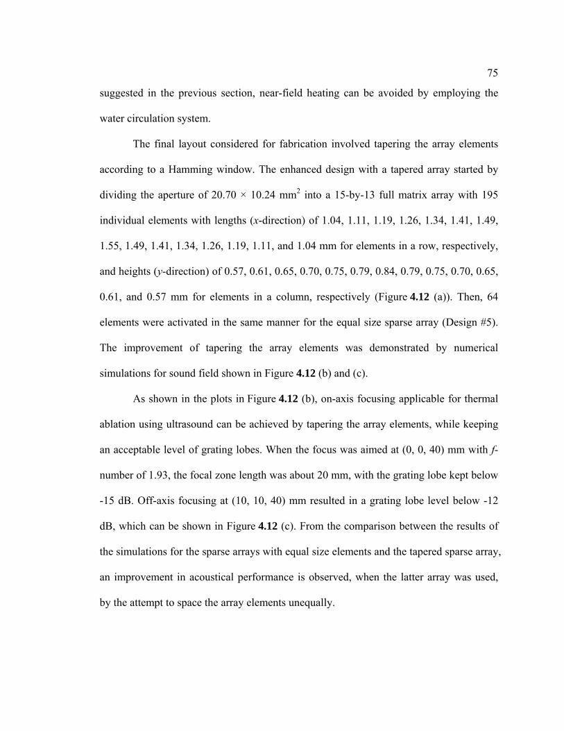
75
suggested in the previous section, near-field heating can be avoided by employing the
water circulation system.
The final layout considered for fabrication involved tapering the array elements
according to a Hamming window. The enhanced design with a tapered array started by
dividing the aperture of 20.70 × 10.24 mm2 into a 15-by-13 full matrix array with 195
individual elements with lengths (x-direction) of 1.04, 1.11, 1.19, 1.26, 1.34, 1.41, 1.49,
1.55, 1.49, 1.41, 1.34, 1.26, 1.19, 1.11, and 1.04 mm for elements in a row, respectively,
and heights (y-direction) of 0.57, 0.61, 0.65, 0.70, 0.75, 0.79, 0.84, 0.79, 0.75, 0.70, 0.65,
0.61, and 0.57 mm for elements in a column, respectively (Figure 4.12 (a)). Then, 64
elements were activated in the same manner for the equal size sparse array (Design #5).
The improvement of tapering the array elements was demonstrated by numerical
simulations for sound field shown in Figure 4.12 (b) and (c).
As shown in the plots in Figure 4.12 (b), on-axis focusing applicable for thermal
ablation using ultrasound can be achieved by tapering the array elements, while keeping
an acceptable level of grating lobes. When the focus was aimed at (0, 0, 40) mm with f-
number of 1.93, the focal zone length was about 20 mm, with the grating lobe kept below
-15 dB. Off-axis focusing at (10, 10, 40) mm resulted in a grating lobe level below -12
dB, which can be shown in Figure 4.12 (c). From the comparison between the results of
the simulations for the sparse arrays with equal size elements and the tapered sparse array,
an improvement in acoustical performance is observed, when the latter array was used,
by the attempt to space the array elements unequally.

76
(a) Design #6 – Aperture size: 20.70 × 10.24 mm2 (15-by-13)
(b) Focal point aimed at (0, 0, 40) mm (c) Focal point aimed at (10, 10, 40) mm
Figure 4.12: (a) Scheme of the tapered phased array with periodically sparsed elements (Design #6) and simulation results of the ultrasound field of the normalized intensity for (b) on-axis focusing and (c) off-axis focusing plotted as a contour with levels indicated at 0, -1, -2, -3, -6, -9 and -12 dB, as indicated from the intensity color bar.
Grating lobe
The distribution of the reduced number of elements in the sparse array can be
optimized by using different methods to achieve acceptable properties for the radiation
pattern. However, further investigation along these lines is beyond the scope of the
current research. Among the suggested array models for this research, the layout (Design
#6) shown in Figure 4.12 (a) is expected to provide the most reliable model that can both

77
assure the accurate ultrasound focusing for heart ablations, and permit straightforward
fabrication. Based on the numerical simulation results of transducer arrays, the
fabrication of the transducer array with an acoustic matching layer is discussed in
Chapter 5.
4.3 Temperature distribution computations
The purpose of this section is to discuss the bio-heat transfer model, the
computational methods and the numerical issues that have been observed in the
development, and the application of these processes to the design of the ultrasound
applicator. The calculations used to simulate heating from the focused ultrasound arrays
were developed using a numerical solution to the bio-heat transfer equation (BHTE)
(Pennes, 1998), which is shown in the previous chapter (Equation 3.4.) An explicit, three-
dimensional finite-difference solution to the BHTE was implemented in MATLAB®.
4.3.1 Numerical methods for bio-heat transfer equation
4.3.1.1 Finite Difference Method (FDM)
The ultrasound pressure field radiating from the transducer array was calculated
using analytical methods while the bio-heat transfer equation (BHTE) was solved using a
numerical method with initial conditions and boundary conditions. The finite difference
method translates the differential equation into a difference equation that can be analyzed
numerically. The generation of a mesh is required to define local coordinate surfaces.

78
Then the unknown function values are found from the difference equations for each mesh
node. For the implementation of the method using MATLAB®, a well-known
computational technique, the finite-difference time-domain (FDTD), is adopted. It can
solve the heat transfer equations using an explicit finite difference method in a leapfrog
manner. The FDTD has been used in much geometry to accurately simulate heat transfer
processes in thermal analysis. Numerical modeling of heat transfer in the myocardium
was carried out with first order differences in time and second order differences in space.
For a finite difference scheme, a grid in the (x, t) plane is laid out with grid points
and , where xjx j ∆= tnt n ∆= 0, >∆∆ tx are small enough to avoid grid dispersion
(computational artifact) and j and n are integer.
The simplest parabolic partial differential equation is the 1-D heat equation
xxt ucu 2= . (4.9)
In order to apply the FDTD to the BHTE in tissue ablation models, Equation 4.9 must be
written with the blood perfusion term and thermal source term in 3-D. Substituting
difference approximations into the BHTE, and solving this for Tn+1, the temperature at
time level n+1 leads to an explicit finite difference method:
( ) ( )( ) ( ) q
CtTTwC
CtTTTr
TTTrTTTrTT
ta
nkjib
t
nkji
nkji
nkjiz
nkji
nkji
nkjiy
nkji
nkji
nkjix
nkji
nkji
ρρ∆
+−∆
−+−+
+−++−+=
−+
−+−++
,,1,,,,1,,
,1,,,,1,,,1,,,,1,,1
,,
2
22,
txxx Cz
try
trx
trρκαααα
=∆∆
=∆∆
=∆∆
= ,,, 222 ,
(4.10)
where, is the temperature [°C] at time t [s], C( tzyxTT ;,,= ) t is the specific heat of the
tissue [J·kg-1·°C-1], Cb is the specific heat of the blood [J·kg-1·°C-1], κ is the thermal

79
conductivity [W·m-1·°C-1], Ta is the blood temperature [°C], and r is a constant related to
the numerical stability.
4.3.1.2 Initial and boundary conditions
Because the heat transfer equation involves both a time and a space solution to
Equation 4.10, boundary conditions at x = 0 and x = d, for instance, and initial conditions
at t = 0 must be specified. Since the PDE involves a first-order time derivative, the initial
condition at one time-step is required. The initial temperature is taken to be T1j = 37 °C
which is normal body temperature. With regard to the boundary conditions in one-
dimensional problems, there are several common possibilities that are simply expressed
in mathematical form. The simplest boundary condition is the Dirichlet boundary
condition or the boundary condition of the first kind:
0TTboundary
= . (4.11)
The temperature is held fixed at a constant temperature (e.g. ) at the
boundaries. The second condition corresponds to the existence of a fixed or constant heat
flux at the boundaries. It is called as Neumann boundary condition or the boundary
condition of the second kind, which is mathematically expressed as
C3701 °== TTn
0=∂∂
boundarynT , (4.12)
where n represents the coordinate that is normal to the boundary. The Neumann condition
is implemented by setting the endpoint value equal to the point next to it: 12 nn TT = ,

80
which implements the thermal insulation conditions. Implementing this boundary
condition on the finite difference grid using a forward difference approximation for the
derivative leads to the relationship x1 = x2, where x1 is a point on the grid boundary.
Lastly, the Robin condition or the boundary condition of the third kind represents the
case where the heat flows out of the control volume. For the myocardial ablations, a
convection surface condition should be considered at the endocardium because of the
convective cooling due to the flowing blood in the chamber of the heart. Mathematically
this condition can be expressed as
( )boundary
bboundarya nTkTTh∂∂
−=− , (4.13)
where h is called the heat-exchange coefficient and is largely dependent on the velocity
of the blood flow in that region. The values of h = 4000 W/m2·K and h = 100 W/m2·K are
typical of the heat-exchange coefficient at the endocardial surface and the epicardial
surface, respectively (Bhavaraju, 2000). Figure 4.13 shows boundary conditions for the
heat transfer equation in soft tissue at various types of boundaries.

81
T(x, t)T(x, t)T(x, t)
T0
x x x
T(0, t)
Ta, h
(a) First kind (b) Second kind (c) Third kind
Figure 4.13: Boundary conditions for the heat transfer equation in soft tissue at various types of boundaries. (Incropera and De Witt, 1990)
4.3.1.3 Stability requirement
The solutions to the three-dimensional bio-heat transfer equation (Equation 4.10)
subject to the initial and boundary conditions are all bounded. For the FDTD method
using forward time, centered space (FTCS) scheme, if ∆t is too large, unstable solutions
that oscillate and grow can be obtained. The FTCS scheme yields stable solutions only if
the constants related to the numerical stability in each direction satisfy a simple criterion
that sets a limit on the calculation time step. The constant in the x-direction with a
criterion for the stability of explicit FDTD method is expressed as Equation 4.14.
21
2 <∆∆
=xt
Cr
tx ρ
κ (4.14)
82
4.3.2 Simulations of thermal distribution: Thermal ablation
4.3.2.1 Introduction
As reviewed in Chapter 3, the convective heat transfer caused by the blood
perfusion dominates the heat dissipation in tissue. However, the heat convection between
myocardium and blood within the atrium occurs as direct energy transfer rather than by
blood perfusion. The blood flow is a heat sink at the endocardium (inner wall of the
heart) in the treated volume. Therefore, the boundary conditions for convection term in
the bio-heat equation have to be considered. The thermal model of the myocardium along
with further consideration of the calculation of the thermal distribution as well as thermal
dose requirements for the cardiac tissue ablations are discussed in this section.
4.3.2.2 Thermal model of the tissues
The level of blood perfusion used in this study (5.3 kg·m-3·s-1) was kept constant
until the critical temperature was reached (50°C). Above this temperature, the perfusion
was dropped to zero for the remainder of the treatment (Tyreus and Diederich, 2002),
thus simulating the cessation of blood flow in coagulated tissue due to the destruction of
blood vessels. The ultrasound power deposited in tissue was obtained from the acoustic
pressure distribution, which is shown in Equation 3.5. The assumption was made in the
acoustic calculations that the attenuation and absorption of ultrasound were constant
throughout the treatment. Other relevant physical parameters used in the calculations are
listed (Table 4.2.)

83
Table 4.2: Physical parameters used in acoustic calculations and biothermal simulations
Parameter Value Reference
Density (ρ) 1000 kg·m-3
Specific heat capacity (Ct) 3700 J·kg-1·°C-1
Perfusion (w) 5.3 kg·m-3·s-1 (Xu et al., 1998)
Thermal conductivity (κ) 0.5W·m-1·°C-1
Attenuation (µ) 1.5 dB·cm-1·MHz-1 (Worthington et al., 2002)
Speed of sound (c) 1500 m·s-1 (Worthington et al., 2002)
4.3.2.3 Computational results and analysis
Temperature simulations were used to verify the potential to increase the tissue
temperature to about 50°C with ultrasound energy. Simulation results of the thermal
distribution, as indicated from the temperature color bar, in the cardiac tissue and the
temperature rise estimation near the focal region are shown in Figure 4.14 and
Figure 4.15 for ex vivo and in vivo, respectively. Ex vivo analysis without blood perfusion
was performed according to Equation 3.4, but assumed that the blood perfusion rate in
tissue was zero, since explanted tissue was used the blood flow could not be recreated.
Any effect of blood flow on the temperature distribution in the tissue was therefore
ignored.
Figure 4.14 (a) illustrates that the temperature changed more rapidly in the ex vivo
conditions rather than for the in vivo conditions shown in Figure 4.15 (a). The trend
demonstrated that with higher maximum temperature was achieved with lower sound

84
intensity. During the exposure period, the calculated temperature rose from 37.0 to 56°C
for ex vivo condition and from 37.0 to 55°C for in vivo condition, respectively in 280
seconds. The lesion size of achieved in explanted tissue (Figure 4.14 (b)) was expected to
be bigger than Figure 4.15 (b) due to the removal of the heat dissipation effects of blood
flow found in the body. This illustrates the effect of blood perfusion on lesion size. Using
Equation 3.4, the blood perfusion rate in tissue was calculated as 5.3 kg·m-3·s-1. On-axis
focusing at (0, 0, 30) mm from the geometrical center of the array and a peak sound
intensity at the focal point of 70 W/cm2 was required to achieve similar results to those
from ex vivo simulation (50 W/cm2) in addition to a slightly higher intensity at focal point.
With these simulations, lesion size (described with dotted lines in Figure 4.14,
4.15 (b), which are the isothermal lines at 50°C) and required sonication time can be
calculated. More reliable prediction of thermal distribution in the myocardium can be
performed with proper boundary conditions at epicardium and endocardium.

(a) Temperature histor
(b) Thermal distribution w
Figure 4.14: Simulation results of (a) temperatlocation of the focal point and (b) the thermavivo with peak sound intensity at the focal poin
Array turned off
y at the focal point
ithin the cardiac tissue
ure as a function of time calculated at the l distribution within the cardiac tissue (ex t of 50 W/cm2).

86
(a) Temperature histo
(b) Thermal distribution w
Figure 4.15: Simulation results of (a) temperalocation of the focal point and (b) the thermvivo with peak sound intensity at the focal poi
Array turned off
ry at the focal point
ithin the cardiac tissue
ture as a function of time calculated at the al distribution within the cardiac tissue (in nt of 70 W/cm2).

Chapter 5
Transducer probe fabrication
As discussed in previous chapters, a transesophageal ultrasound applicator must
be small enough to fit into the esophagus. It must also avoid damage to the esophagus
while being inserted. In order to reduce the size of the transducer, piezoelectric ceramics
(PZT-8, Navy Type III) able to handle the large electric power needed for tissue ablation
were designed to operate at a frequency of 1.6 MHz. The current research suggests a
design of a sparse phased array to deliver sufficiently high intensity to create lesions in
tissue as well as to enable the ultrasound beam to be steered without moving the
applicator in the esophagus. To verify the array design with either the exposimetry
measurements or the ex vivo tests, it is necessary to build and assemble the array with an
appropriate housing.
In order to ensure the required maximum power transfer from each array element
to the ablation target, an acoustic impedance matching layer with a quarter wavelength
thickness was designed and constructed. Also, LC (L: inductor; C: capacitor) circuits for
electric impedance matching to the value of 50 Ω∠0° between the ultrasound driving
system and each element were constructed. A water circulation system was installed in
the applicator to cool down the high temperature in the acoustic near field to reduce
unwanted heating to the esophagus and surrounding tissues. An acoustic window was
devised to minimize the loss of the acoustic energy passing through the housing as well
as to keep cooling water in the applicator system during the circulation. The effect of the
88
acoustic window on the array performance was simulated by calculating the ultrasound
field from the transducer array.
In this chapter, design and development issues, the fabrication process, and the
results and analyses of the sparse phased ultrasound array are presented in detail.
5.1 Transducer array construction
Based on the simulation results of the ultrasound field from the transducer array, a
prototype of the array was designed and built in-house. The fabrication of the transducer
array and its related issues such as acoustic impedance matching and wiring of the
elements are presented in this section. Also, phase matching for precision beam forming
is demonstrated.
5.1.1 Materials for the array
Since the properties of the material are crucial factors affecting the performance
of the ultrasound treatment, choosing an appropriate material for the ultrasound
transducer array was carefully considered. A family of ceramics made from lead
zirconate and lead titanate (PZT) have been used in medical ultrasonic transducer design
for the past three decades. The major advantages of PZT are the high electromechanical
coupling coefficient in thickness mode, high relative dielectric constant, and low
mechanical and dielectric loss tangents. Table 5.1 shows some of the properties,

89
considered as important factors for transducer design, of piezoelectric ceramics used in
medical ultrasonic transducer.
Table 5.1: Comparison of the properties between piezoelectric ceramics.
Material Type Parameter
PZT-4 PZT-5A PZT-8 Thickness coupling factor, kt 0.573 0.486 0.480
Dielectric constant 1150 1800 1000
Mechanical dissipation factor, tanδ 0.002 0.013 0.002
Mechanical quality factor, Q 500 75 1000
Density [kg/m3] 7500 7750 7500
PZT-5A is recommended for diagnostic (imaging) transducers due to its high
sensitivity and high time stability. PZT-4 and PZT-8, however, are recommended for
high intensity ultrasound transducers with an advantage of a higher mechanical quality
factor. Thus, PZT-8 was chosen as the material of the transducer array, since it can
handle the high electric power required for tissue ablation.
One disadvantage of a piezoelectric ceramics is its high acoustic impedance (34
MRayls) compared to human tissue/water (1.5 MRayls). Because of the acoustic
impedance mismatch, sound waves radiating from the ceramic transducer and entering
the tissue/water may be strongly reflected. If so, only a small amount of the acoustic
energy would be delivered into the tissue. In order to improve the efficiency of the

90
transducer, a matching layer(s) having an intermediate impedance can be placed between
the ceramic and tissue/water.
5.1.2 Array construction
The periodic sparse and phased array design for cardiac ablation has 64 active
elements operating at a frequency of 1.6 MHz. The active elements selected from a total
195-element (15 × 13) rectangular grid are spatially sparse. The tapered plane elements
consist of a thin piezoelectric ceramic, operated at a resonance that is determined by the
thickness resonance frequency (λ/2) of the ceramic.
A series of array fabrication procedures have been completed in-house. These
include lapping the ceramic, sputtering the chromium and gold, building the acoustic
matching layer, and dicing and cabling the elements. First, a lead zirconate titanate
ceramic (PZT-8, TRS Ceramics, State College, PA) was diced to 20.70 × 10.24 mm2 and
lapped to a thickness of 1.4 mm corresponding to the resonance frequency of 1.6 MHz.
The ceramic has electrode surfaces coated with chromium and gold sputtering. An
acoustic impedance matching layer was coated on the surface that radiates ultrasound into
the tissue/water. Then, the ceramic was completely diced through its thickness to form a
64-element sparse phased array and attached securely to the frame using silicone with a
primer. A sketch representing a back view of the 15-by-13 linear tapered array is shown
in Figure 5.1. All the cuts were accomplished by dicing the ceramic with a kerf (having
distance between the adjacent elements, which represents the thickness of the cutting

91
blade) of 105 µm using a dicing saw (Model 982-6, Kulick and Soffa Industries, Willow
Grove, PA.)
0.105
Kerf
0.105
Element
Unit: mm
1.114 1.263 1.411 1.550 1.411 1.263 1.114
.570
.653
.747
.840
.747
.653
.570
.607
.700 .793 .793 .700
.607
1.040 1.189 1.337 1.486 1.486 1.337 1.189 1.040
20.70
10.24
Figure 5.1: A diagram showing a back view of the 15-by-13 linear tapered array with total size of 20.70 × 10.24 mm2. The diced face of the ceramic was completely cut through its thickness. An enlarged representation of the elements shows that the distance between the adjacent elements is 105 µm, which represents the thickness of the cutting blade.

92
Figure 5.2 shows the prototype array after dicing but before soldering wires to the
ceramic elements. It includes 64 active elements selected based on the simulation results.
Figure 5.2: The photograph of the including 64 active elements periodi
m
m
5.1.3 Acoustic impedance matchin
In spite of the ability of the
high acoustic impedance (34 MRa
decreased the efficiency of deliveri
mismatch at the interface of the tran
transmission and an increased intern
By introducing an intervening mater
20.70 m
10.24 m
prototype array after dicing into 15-by-cally sparse.
g
piezoelectric ceramic to handle the hig
yls) compared to human tissue/water (1
ng the high power into soft tissue. The
sducer and human body/water results in
al reflection of the sound waves from th
ial with an appropriate thickness as a ma
Kerf
13 elements
h power, its
.5 MRayls)
impedance
a decreased
e transducer.
tching layer,

93
higher transmission of ultrasound energy from the ceramic through the intermediate layer
and into the tissue/water increased the output pressure of the array compared to the output
without an intermediate layer. An acoustic quarter-wavelength matching layer, acting as a
mechanical transformer, was interposed between the ceramic and the tissue/water. The
thickness and material of the matching layer were chosen based on a solution to a three-
layer (ceramic, matching layer, and tissue) problem.
A single impedance matching layer was built on top of the array for improved
transmission of ultrasound energy for the thermal ablation of the cardiac tissue. First a
frame for casting the matching layer on the surface of the transducer face was fixed onto
the PZT-8 piece with an adhesive primer. Thin oxidized silver (Powder, 2-3.5 µm, 99.9+
%, Aldrich, Milwaukee, WI), which has an acoustic impedance of 7.3 Mrayls, was
poured on the surface. The matching layer was a 2:1, mixture of Insulcast 501 epoxy
(Insulcast, Roseland, NJ) and silver powder. In order to separate the epoxy layer from the
silver-conducting layer, the whole assembly was centrifuged for 10 minutes (the
orientation of the array surface was parallel to the axis of rotation) and cured overnight.
Then, the upper layer of cured epoxy was sanded out, and the surface of the silver layer
lapped to the designed quarter-wavelength thickness of 0.297 mm.
5.1.4 Cables
The specifications of the cables for connecting the array elements and the
ultrasound driving/amplifier system were determined by the capacitance of the ceramic
element in the array. This capacitance depends on the thickness, electric permittivity, and

94
the area of the radiating surface of the element. Since the element surface area of the
medical ultrasound transducer is generally small, coaxial cables with low capacitance
have been widely used in medical ultrasound transducer arrays.
The 64 active elements were soldered to MRI compatible, 42 AWG, 30 pF/ft
miniature coaxial cables (Precision Interconnect, Portland, OR) 2.5 m long. The
connector between the other ends of the cables and the driving/amplifier system used a
ZIF (Zero insertion force) connector (ITT Industries, Cannon, Santa Ana, CA). As
described in previous sections, the transducer array for the current study has extremely
small elements, which makes soldering the coaxial cables to the individual elements
difficult. Thus, the cables were soldered to the ceramic elements using a micro-tip
soldering pin at low temperature (less than the Curie temperature of PZT-8) with the
assistance of a microscope. Figure 5.3 shows the prototype array after soldering wires to
the ceramic elements. It includes 64 active elements selected based on the simulation
results. Note that the mass of solder on the element’s rear side was ignored in the
calculations. The soldering temperature was kept below 500°F to prevent any damage to
the piezoelectric ceramic.

95
Figure 5.3: The photograph showing the back view of transducer array with coaxial cables.
5.1.5 Phasing for focusing
For this study, a two-dimensional ultrasound phased array was designed and
fabricated in-house. The ultrasound beam generated from a phased array can be
controlled by electrically steering the focal point from one location to another by
changing the phase and power of the individual elements of the array. For precision
setting of focal points from the prototype array, manual phasing for four different focal
points, (0, 0, 30), (0, 0, 25), (0, 0, 20), and (0, 5, 30) mm, from the geometrical center of
the array were arranged.

96
5.2 Electrical matching
The transducer array was driven by an ultrasound pulse generator with an
amplifier system (UDS 2050PA, Advanced Surgical Systems Inc., Tucson, AZ) that has
50 Ω impedance output. The ultrasound driving system is capable of delivering up to 12.5
W per channel with a ±1° phase resolution each. The driving system is controllable
through software, by which the amplitude and phase of the driving signal from each
channel can be set. When the array is connected to the driving system, each ceramic
element acts principally like a capacitor. To obtain maximum power transfer from the
transducer to the ultrasound driving system is necessary to match the electrical
impedance of the array elements to the output impedance of each channel of the driving
system.
To match the electric impedance of the array elements in water to the driving
system, individual LC (inductive-capacitive) circuits, that allow the transducer driving
system to achieve a 50Ω∠0° input impedance, was built for each of the 64 elements. The
impedance of the matching circuit was adjusted by varying the value of the capacitance
and the number of turns of coils. To find the necessary values for an inductor (L) and
capacitors (C), the impedances of the array elements at the operating frequency were
measured using a network analyzer (E5100A, Agilent Technologies, Englewood, CO).
Then the tuning capacitance and inductance for each element can be determined using a
Smith chart or a commercial program for RF circuit design. By changing either the
number of turns of a toroidal inductor or the value of the capacitor, it is possible to adjust
the magnitude and phase of the impedance. A series of trials were made to find the

97
inductance and capacitance values to achieve an impedance of the array of 50Ω∠0°.
Figure 5.4 shows the impedance matching circuit board used for the current research. 64
matching circuits were built, one for each element.
Figure 5.4: Photograph of one of 16 matching circuit boards for the prototype array. One circuit board includes 4 channel matching circuits.
5.3 Probe housing
5.3.1 Housing
The probe head must be strong enough to avoid failure of the probe and to
provide a secure and stable housing for the array. The probe housing is composed of a
main housing body, an acoustic window, cooling pipes, connectors, and a flexible

98
insertion tube. Listed below are the materials used for the probe head housing and
cooling system.
Probe head housing materials
- Housing body, ceramic frame, nose-cone, and connectors: Delrin®
- Acoustic window (acoustically transparent): Polyurethane
- Cooling tubing: Copper (within the probe head) and Rubber (within the
insertion tubing)
- Insertion tubing: Silicone
- Sealing: Polyurethane form (spray) and sealing tape
All the parts of the housing were built in the machine shop in The Bioengineering
Department of PSU using material compatible with magnetic resonance imaging (MRI.)
Since the current applicator may be used with an MRI for imaging-guided focused
ultrasound surgery, Delrin® and copper were chosen for the housing. The housing holds
the ultrasound array in a rectangular frame and includes water circulation for the cooling
system. An acoustic window for the probe head housing was constructed in-house using
polyurethane. The acoustic window is attached to the housing shown in Figure 5.5. As an
alternative, a latex membrane, which forms a bolus of water surrounding the array, could
be used instead of an acoustic window.
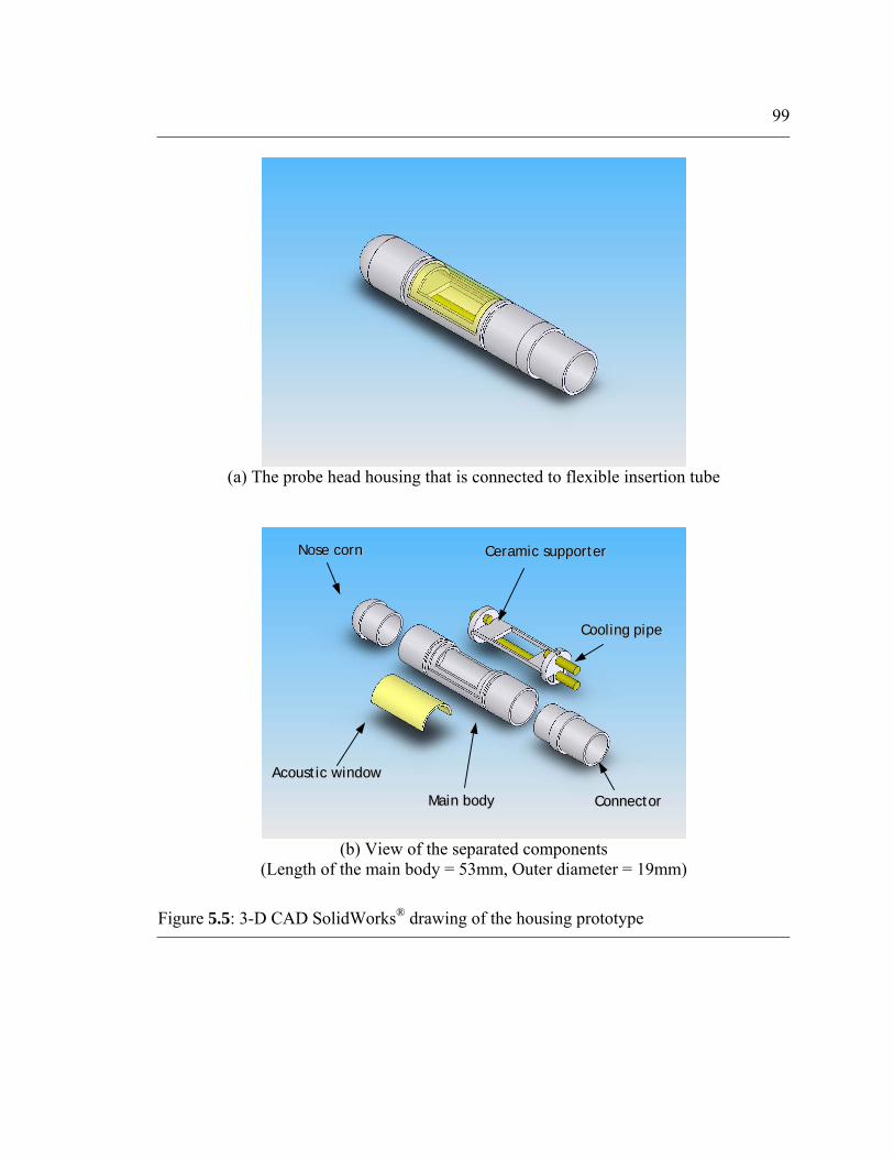
99
(a) The probe head housing that is connected to flexible insertion tube
(b) View of the separated components
(Length of the main body = 53mm, Outer diameter = 19mm)
Figure 5.5: 3-D CAD SolidWorks® drawing of the housing prototype
NNoossee ccoorrnn CCeerraammiicc ssuuppppoorrtteerr
MMaaiinn bbooddyy
CCoooolliinngg ppiippee
CCoonnnneeccttoorr
AAccoouussttiicc wwiinnddooww

100
5.3.2 Acoustic window
Even though a latex membrane, intended to create a bolus of water around the
transducer array, would provide good coupling for the esophageal wall, a solid acoustic
window for the probe head was used to provide a more secure and stable housing for
sonication in the esophagus. The window material should have a specific acoustic
impedance close to that of water (Z = 1.5 MRayls, c = 1500 m/s), so as to be acoustically
transparent. Also, it should be designed to avoid extreme refraction of the ultrasound
beam due to the different acoustical properties between the cooling water and the
window, and the window and the esophageal wall.
Refracted rays due to the different speed of sound between mediums
Cooling water
Acoustic window
Tissue Array
Ultrasound ray froman element Thickness
of thewindow
Ablation target
Figure 5.6: Illustrations of the refraction of the ultrasound ray due to the acoustic window
(Water: Z = 1.5 MRayls, c = 1500 m/s; TPX®: Z = 1.78 MRayls, c = 2170 m/s; Tissue: Z = 1.5 MRayls, c = 1500 m/s)

101
If the propagation speed in the window is different than that in the cooling water
or in the esophageal wall, acoustic waves will refract and may generate unwanted
focusing. Currently TPX® is one of the most popular materials for the acoustic windows
for medical ultrasound applicators. To simulate refraction of the ultrasound beam due to
the acoustic window, a half-cylindrical window of TPX® (Z = 1.78 MRayls, c = 2170
m/s) was modeled (see Figure 5.6.) Then, the refraction angles were calculated according
to the height of each array element and compared to two different thickness of the
window. The simulation results are shown in Figure 5.7.
Figure 5.7: Simulation results of the refracted angle at the outer surface of the housing according to the heights (h1) of the transducer array elements.
The resulting ultrasound rays are illustrated in Figure 5.8 for the cases of 1 mm
and 2 mm thick windows.

102
Unwanted focus due to acoustic window
h1 ....
(a) Thickness of the window, t = 2 mm
....
(b) Thickness of the window, t = 1 mm
Figure 5.8: Illustration of the resulting ultrasound rays due to the refracted ultrasound beam for the different thickness of the windows.
As shown in Figure 5.7 and Figure 5.8, the thicker windows lead to greater
refraction. The extreme refraction shown in Figure 5.8 (a) could lead to heating and
damage of the esophageal wall. Consequently, the thickness of the cylindrical window
should be selected carefully. There are many suitable materials for the acoustic window.
Polyurethane (RP-6410) is one of the acceptable choices because it has properties (Z =

103
1.49 MRayls, c = 1550 m/s) very similar to those of water. Although an acoustic window
made of polyurethane may be too soft to maintain secure and stable housing compared to
TPX®, polyurethane was chosen because it is more easily formed into the shape required.
5.4 Water circulation system
A water circulation system was installed in the ultrasound applicator. This
continuous water-flow cooling system was designed to reduce the transducer surface
temperature in order to minimize local heating of tissue. In addition, degassed water
filled the empty space between the array and esophagus for a better impedance matching.
Figure 5.9: Photograph of the assembled probe head w
m
The water circulation system consists of wa
housing, a gear pump driver (Model 75211-21 and 7
Water tube
53 m
Φ 19 mm
ith water circulation tubes
ter tubes embedded in the probe
5211-22, Cole-Parmer Instrument

104
Company, Vernon Hill, IL), and a bubble trap chamber. Two types of tubing, copper
(within the probe head) and rubber (outside of the probe head), are MRI compatible and
used to circulate water over the array. Figure 5.9 shows the assembled probe head with
water circulation tubes.
Lastly, Figure 5.10 shows the completed transesophageal ultrasound applicator
with the insertion tube including cables inside, the ZIF connector that connects to the
amplifier system, and water circulation tubes. The ultrasound applicator fabricated in-
house was tested for the verification of the suggested design of the sparse phased array
using exposimetry and ex vivo experiments. Through these experiments, the feasibility of
using the transesophageal applicator for the cardiac ablation by ultrasound array was
evaluated.
Figure 5.10: Photograph of the constructed transesophageal ultrasoundthe insertion tube including cables inside, the ZIF connector, and water ci
Probe head
Water
circulation tube
ConnectorInsertion tube
applicator with rculation tubes.

Chapter 6
Experiments for ex vivo evaluation
For the verification of the suggested design, the sparse phased array with an
acoustic impedance matching layer was constructed, and evaluated using exposimetry
and ex vivo experiments. As a preliminary experiment, ultrasonic exposimetry was
performed to determine the focusing and steering characteristics of the array.
Furthermore, these measurements show that the experimental results correlate well with
theory. Also, ex vivo experiments using fresh tissue were used to ensure that the array is
capable of delivering sufficient acoustical power to create lesions in tissue. Through the
experiments, the feasibility of transesophageal treatment of arrhythmia by ultrasound
array was evaluated.
6.1 Preliminary experiments: Exposimetry
6.1.1 Introduction
Ultrasound is a propagated wave of mechanical energy. Exposure to this acoustic
energy can generate thermal lesions in soft tissue for treatment or it can produce harmful
physical effects in tissue. Therefore, there is a great demand for methods to examine the
generation and detection of the energy introduced into the body from ultrasound
equipment. For the current research, calibration of the ultrasound field generated by the
transducer array is necessary in order to ascertain that there is no damage to the tissue in

106
the acoustic near field. Moreover, the beam focusing and beam steering to a target point
should be evaluated with common exposure parameters such as acoustic pressure,
intensity, and power to ensure thermal ablation.
One method of measuring the acoustic pressure field generated from an
ultrasound transducer array using an exposimetry system is the precision calibration of
the probes. Ultrasonic exposimetry refers to quantitative and accurate measurements of
the spatial and temporal distributions of the exposure parameters, usually propagation in
water. Exposimetry measurements are useful in determining where the focal point is, how
the acoustic intensity is distributed spatially, and how the acoustic energy is distributed in
the area near the array face. Figure 6.1 shows the photograph of the experimental
apparatus for exposimetry.
Figure 6.1: Experimental apparatus for exposimetry. The array and hydrophone are held in a water tank.

107
6.1.2 Experimental setup
To determine the acoustic field generated by the phased array prototype, an
exposimetry system (Figure 6.1) was equipped with an automated computer-controlled
scanning and data acquisition system. The scanning system (Velmex Inc., Bloomfield,
NY) can position a hydrophone throughout the 1D/2D acoustic field in a water tank. As
shown in Figure 6.2, a PC was connected to a four-motor positioning system via an
RS232 serial port. A needle type PVDF hydrophone (SN: 679, Precision Acoustic Ltd,
Dorchester, UK) was submerged in an anechoic tank (120 × 50 × 52 cm3) containing
degassed distilled water (room temperature, approximately 20°C) instead of regular tap
water. To minimize cavitation, a customized degasser, built in-house, was utilized to
reduce the dissolved oxygen content of the distilled water to 1-2 ppm.
Using the hydrophone and the digital oscilloscope, the ultrasound fields from a
transducer array were measured and characterized. The hydrophone was connected
through a pre-amplifier to the digital oscilloscope. The PC also interfaced via a GPIB
card with the oscilloscope (54622A, Agilent Technologies, Palo Alto, CA), which
captured the voltage amplitudes detected by the hydrophone. Programs for automated
control of the motors and data acquisition from the oscilloscope were written using Quick
Basic (Microsoft Corporation, Redmond, WA). The phased array submerged in the water
tank was connected to a 64-channel amplifier with LC (inductive-capacitive) electrical
matching circuits for each channel. Another PC controlled the parameters of each channel
of the amplifier and an ultrasound pulse generator varying the frequency, phase, and
input driving power.

108
Array (Transmitter)
Hydrophone
Anechoic water tank
DC Coupler
DC Voltage supplier (28 V)
Oscilloscope
PC #1
GPIB
64-ChannelAmplifier
Position Controller
RS232
RS232
z (dir-1)
y (dir-2)
x (dir-3)
PC #2
Figure 6.2: Schematic diagram of the experiment setup used in exposimetry measurement of the sound pressure field from the ultrasound array.

109
6.1.3 Results and analysis
The input power to the transducer elements for the exposimetry measurement was
0.5 - 2 W for each channel at 1.6 MHz. Note that during the exposimetry, the level of the
input power was carefully controlled to avoid damage to the measurement hydrophone
and pre-amplifier due to excessive high sound pressure. The hydrophone (receiver) was
located at three pre-selected focal points in the acoustic field, (0, 0, 30), (0, 0, 20), and (0,
5, 30) mm, from the geometrical center of the transmitter array. Then sound pressure data
was acquired and stored using the digital oscilloscope. The one-dimensional pressure
measurements were made in either the x-direction (dir-1, lateral) or the y-direction (dir-2,
longitudinal) between -30 and +30 mm as well as in the z-direction (dir-3, axial) between
10 and 50 mm from the surface of the array (step size = 0.5 mm). Meanwhile, the two-
dimensional sound pressure data at either the xy-plane between -20 mm and +20 mm of
each direction or the xz-plane between -20 mm and +20 mm of the x-direction and
between 10 mm and 50 mm of the z-direction from the maximum pressure point was
acquired and stored (step size = 2.0 mm). The exposimetry results are shown in
Figure 6.3 through Figure 6.9.
First, the capability of focusing and beam steering at a target point was evaluated
using the exposimetry. The plots of axial or lateral responses are shown in Figure 6.3 and
Figure 6.4 and demonstrate the ultrasound field in the vicinity of the peak intensity. For
on-axis focusing, the center of the focus was measured at the aimed point (0, 0, 30) mm
for both axial and lateral responses. An axial focal zone length (defined as the -3 dB
contour of the peak intensity) of about 16 mm was achieved.
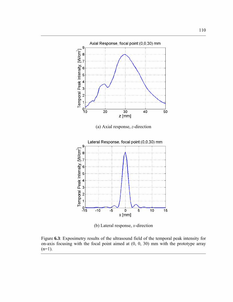
110
(a) Axial response, z-direction
(b) Lateral response, x-direction
Figure 6.3: Exposimetry results of the ultrasound field of the temporal peak intensity for on-axis focusing with the focal point aimed at (0, 0, 30) mm with the prototype array (n=1).
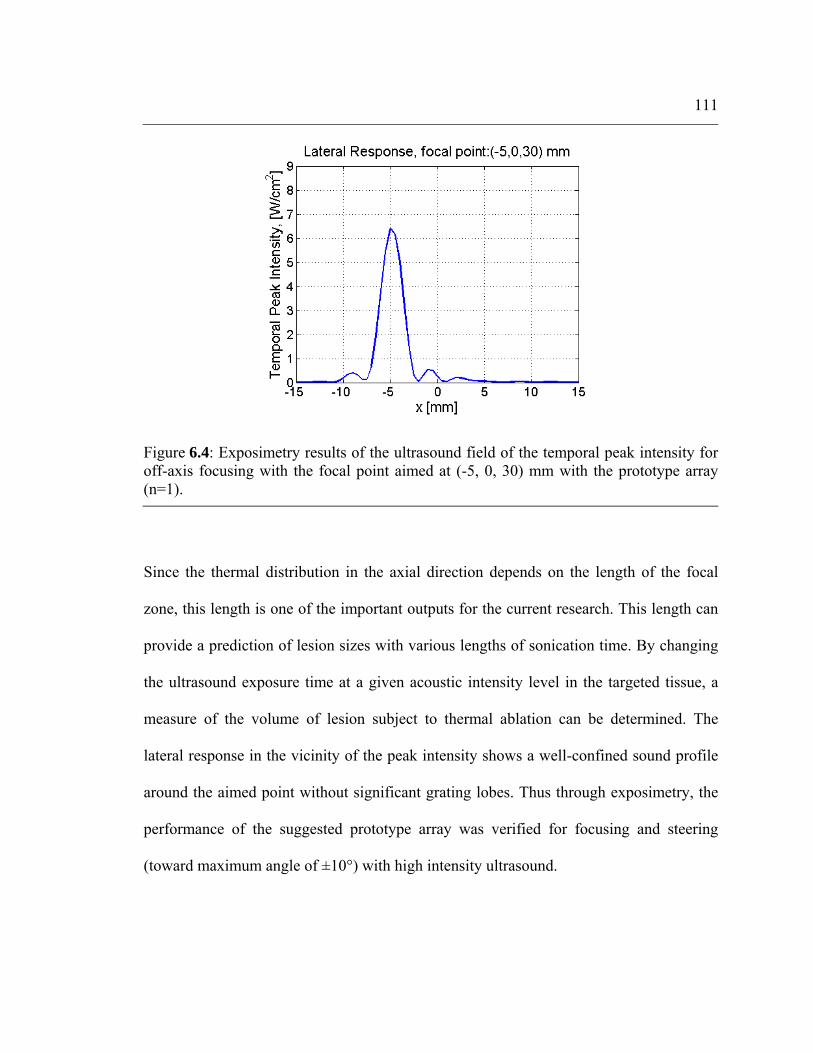
111
Figure 6.4: Exposimetry results of the ultrasound field of the temporal peak intensity for off-axis focusing with the focal point aimed at (-5, 0, 30) mm with the prototype array (n=1).
Since the thermal distribution in the axial direction depends on the length of the focal
zone, this length is one of the important outputs for the current research. This length can
provide a prediction of lesion sizes with various lengths of sonication time. By changing
the ultrasound exposure time at a given acoustic intensity level in the targeted tissue, a
measure of the volume of lesion subject to thermal ablation can be determined. The
lateral response in the vicinity of the peak intensity shows a well-confined sound profile
around the aimed point without significant grating lobes. Thus through exposimetry, the
performance of the suggested prototype array was verified for focusing and steering
(toward maximum angle of ±10°) with high intensity ultrasound.

112
(a) Axial response, z-direction
(b) Lateral response, x-direction
Figure 6.5: Exposimetry results of the ultrasound field of the temporal peak intensity for on-axis focusing either with or without the acoustic window attached to the probe housing (n=1).

113
Further measurements were made to examine the effect of the acoustic window
between the array and targeted tissue (Figure 6.5). The axial and lateral responses of the
peak intensity for on-axis focusing, with (solid line) or without (dashed line) the acoustic
window are shown in (a) and (b), respectively. The sound intensity is slightly lower
around the focal zone when the window is in place. This may be simply due to energy
absorption of the window material. An increase in sonication time or input driving power
can be used to compensate for the loss of the acoustic energy delivered to the targeted
tissue.
Figure 6.6 shows the lateral responses for on-axis focusing with the focal point
aimed at (0, 0, 30) mm with three different driving input powers, 0.5, 1.0, and 2.0 W per
active element. The sound intensities measured at the maximum pressure point were
varied almost linearly with the input driving power. More measurements with greater
levels of input driving power are required to determine the acoustic power for thermal
ablation of tissue. However, sound field measurements with higher input driving power
were not attempted to avoid damage to the hydrophone. A different technique for sound
power measurement, such as the radiation force balance (RFB) principle, should enable
the measurement of focused ultrasound fields driven with higher power (Beissner, 1993).

114
Figure 6.6: Exposimetry results of the lateral responses for on-axis focusing with the focal point aimed at (0, 0, 30) mm with the prototype array. The input driving powers are 0.5-2.0 W/channel and the sound intensities were measured at the maximum pressure point (n=1).
In Figure 6.7 and Figure 6.8, the exposimetry measurements (dashed line) and the
simulation (solid line) of the ultrasound field are compared. For on-axis focusing at (0, 0,
30) mm (Figure 6.7), and off-axis focusing at (-5, 0, 30) mm (Figure 6.8), the maximum
normalized intensity differences between the measurements and the simulations were -10
and -7 dB, respectively. The experimental and theoretical values were matched at their
peak values to make these plots. For both plots, the averaged experimental results show
agreement with the theoretical results.

115
Figure 6.7: Comparison of the results between exposimetry and numerical simulation of the ultrasound field of the temporal peak intensity for on-axis focusing with the focal point aimed at (0, 0, 30) mm with the prototype array (n=4).
Figure 6.8: Comparison of the results between exposimetry and numerical simulation of the ultrasound field of the temporal peak intensity for off-axis focusing with the focal point aimed at (-5, 0, 30) mm with the prototype array (n=4).

116
Lastly, Figure 6.9 shows the experimental results of the two-dimensional
ultrasound fields. The peak intensities for on-axis focusing with the focal point aimed at
(0, 0, 30) mm as well as off-axis focusing with the focal point aimed at (-5, 0, 30) mm
with the prototype array are shown in the xy- and xz-planes, as indicated from the
intensity color bar.
Both on- and off- axis focusing show a cigar shaped focal zone (sound intensity
contour at -3 dB) with a length of 20 mm along either the z-axis or steered axis. Unlike
the one-dimensional sound fields, the two-dimensional result shows grating lobes in the
xy-plane (Figure 6.9 (a)). Since they are located diagonally from the z-axis, they are not
shown in the one-dimensional displays (e.g. Figure 6.3 (b)). The measurements show that
the grating lobe levels are at least 6 dB below the intensity at the focus; serious damage
on normal tissue is not expected.
This section described preliminary experiments to verify and characterize the
developed transducer array. A description of the ex vivo experiments with excised fresh
tissue for thermal ablation will be presented in the following section.

117
(a) xy-plane, z=30mm, on-axis focusing
(b) xz-plane, y=0mm, on-axis focusing (c) xz-plane, y=0mm, off-axis focusing
Figure 6.9: Exposimetry results of the ultrasound field of the temporal peak intensity, as indicated from the intensity color bar, for on-axis focusing with (b) the focal point aimed at (0, 0, 30) mm in xy-plane, (c) in xz-plane, and (d) for off-axis focusing with the focal point aimed at (-5, 0, 30) mm in xy-plane with the prototype array.

118
6.2 Ex vivo experiments
6.2.1 Introduction
In science, ex vivo (Latin: out of the living) experiments are performed in or on
living tissue in an artificial environment outside the organism. For therapeutic ultrasound
studies in living animals, ex vivo tests are usually performed first on isolated soft tissue.
To evaluate the feasibility of using the sparse phased array for cardiac ablation, ex vivo
experiments were performed with extracted fresh tissue. The array and the fresh tissue
were submerged in the degassed phosphate buffered saline (PBS) solution. Then the
ultrasound beam was directed perpendicular to the surface of the tissue. Because the PBS
solution is isotonic and non-toxic to tissue, it can provide the tissue with the same salt
concentration as the normal cells in the body and the blood. The temperature profile in
the focal region of the tissue was measured to ensure that the array can generate the
thermal energy required to create lesions.
Localized thermal ablation of cardiac tissue requires elevating the temperature of
the tissue from the normal body temperature to 50°C. According to a previous study on
the electrophysiologic effect of hyperthermia on cellular excitability, irreversible tissue
injury was observed only at temperatures at or above 50°C. This injury causes loss of
cellular excitability of tissue, which is defined as lack of pacing of the cardiac muscle at
the stimulus level used for regular heartbeat condition. Figure 6.10 shows the distribution
of the median temperature associated with excitability and tissue injury (Nath et al.,
1993). This study predicted that the minimum target area temperature to achieve
permanent blockage of the irregular signal causing AF would be 50°C. For ultrasound
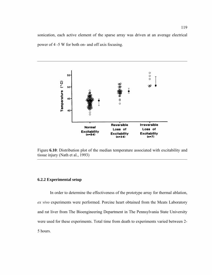
119
sonication, each active element of the sparse array was driven at an average electrical
power of 4 -5 W for both on- and off axis focusing.
Figure 6.10: Distribution plot of the median temperature associated with excitability and tissue injury (Nath et al., 1993)
6.2.2 Experimental setup
In order to determine the effectiveness of the prototype array for thermal ablation,
ex vivo experiments were performed. Porcine heart obtained from the Meats Laboratory
and rat liver from The Bioengineering Department in The Pennsylvania State University
were used for these experiments. Total time from death to experiments varied between 2-
5 hours.

120
Figure 6.11 displays the experimental setup for the thermal ablation
measurements. The array and the fresh tissue were submerged and held in position using
metal clamps. The ultrasound beam was directed perpendicular to the surface of the
tissue. Each element of the sparse phased array was connected to an electrical power
source with a continuous wave (CW) signal at the resonance frequency to achieve the
highest mechanical amplitudes in order to ablate the target tissue in relatively short
periods. An ultrasound driving system (UDS 2050PA, Advanced Surgical Systems, Inc.,
Tucson, AZ) was set to generate the continuous wave at 1.6 MHz for all the experiments.
To measure the temperature in the focal region of the tissue, a thermocouple was
implanted into the tissue at the target point using a 16G 1½ needle (Precision Glide,
Becton Dickinson and Co, Franklin Lakes, NJ). A PC controlling the transducer array
also acquired temperature data from the thermocouple via a data acquisition module
(8018, SuperLogics, Inc, Waltham, MA) and an RS-232 to RS-485 converter.
For on-axis focusing at (0, 0, 30) mm from the center of the array surface, the
array was driven with an average electrical power of 4 - 5 W per element for five
minutes. Water temperature was maintained at 37 ± 1°C using a circulator (Polystat®
12112-00, Cole Parmer, Vernon Hills, IL). The temperature rose from 37°C to 50°C for
two minutes and then remained over 50°C for three minutes. The temperature history at
the focal point is plotted in Figure 6.12 as a function of time. After sonication, the tissue
was dissected at the target area to assess lesion formation. Digital photographs were used
to record the results.

121
Array
Fresh Tissue
Water Tank
Converter module PC
64-Channel Amplifier
Data acquisition module
RS232
z
y x
RS232
Thermocouple
Water pump & Bubble trap
Figure 6.11: Schematic diagram of the experimental setup for ex vivo thermal ablation using the ultrasound phased array.

122
6.2.3 Results and analysis
Figure 6.12 shows the temperature measurement at the focal point in the rat liver.
During the exposure period, the temperature rose from 37.0 to 50.6°C in 120 seconds and
remained between 50.6 and 53.4°C for 160 seconds, causing irreversible tissue injury.
After the transducer array was turned off, the temperature remained over 50°C for 20
seconds due to the heat transfer within the tissue. In order to control the size of the
ablated volume, the temperature distribution in the tissue both during and after ultrasound
application must be considered.
Figure 6.12: Temperature as a function of time recorded at the location of the focal point. The temperature rose from 37 °C to 50 °C for two minutes and then remained over 50°C for three minutes.
Turned off
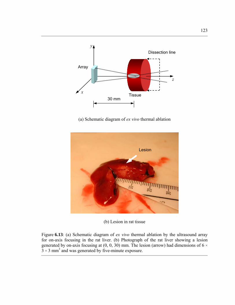
123
x
z
y
Array
Tissue
Dissection line
(a) Schematic
(
Figure 6.13: (a) Schematic diagrafor on-axis focusing in the rat livgenerated by on-axis focusing at (03 × 3 mm3 and was generated by fi
30 mm
diagram of ex vivo thermal ablation
b) Lesion in rat ti
m of ex vivo theer. (b) Photogra, 0, 30) mm. The
ve-minute exposu
Lesionssue
rmal ablation by the ultrasound array ph of the rat liver showing a lesion lesion (arrow) had dimensions of 6 × re.

124
After the rat liver had been exposed to sonication, it was removed from the clamp
and sliced with a scalpel to examine the necrosed region. Lesions were measured several
times using a ruler and a digital photograph was taken. Figure 6.13 shows an ablation
volume created by the sparse phased array in a rat liver sample. The lesion in the tissue
was 6 × 3 × 3 mm3in size. The border between the ablated tissue and the surrounding
tissue can be identified in the photograph taken after five minutes of sonication. This
indicates that the prototype array can deliver sufficient power to the focal point deep
inside the tissue to produce the thermal lesions required for cardiac ablation.
Lastly, in order to evaluate the feasibility of using the developed transducer array
for cardiac ablation, an ex vivo thermal ablation experiment using porcine heart tissue
was conducted. The procedure was the same as for the rat liver tissue.
During the exposure period for ex vivo thermal ablation, the temperature rose
from approximately 37 to over 50°C where irreversible tissue damage was observed
about 160 seconds. Figure 6.14 shows an ablation volume created by the array in a
porcine heart (large photograph: side view; small photograph: top view). A lesion having
dimensions of 6 × 5 × 5 mm3 was created after eight minutes of sonication. The border
between the ablated tissue and the surrounding tissue can be identified in the photograph.
Since myocardial tissue has a more complex structure than liver tissue, a longer exposure
time to complete the thermal ablation is expected. This indicates that the prototype array
can deliver sufficient power to the focal point 30 mm deep inside the tissue to produce
thermal lesions for cardiac ablation. A non-ablated tissue measuring 1.5 mm in diameter
was observed within the lesion, seemingly due to an air gap located front of this volume,
which reflects and scatters the sound from its original path (Smith and Hynynen, 1998).

125
Figure 6.14: Photograph of an ex vivo experimental result son-axis focusing at (0, 0, 30) mm. The lesion (arrow) in po6 × 5 × 5 mm3 and was generated by eight minutes expview).
Also, Figure 6.15 shows an ablation area generated
25) mm. The lesion having dimensions of 4 × 3 mm2 in
after eight minutes of sonication.
Lesion
howing a lesion generated by rcine heart has dimensions of osure (small photograph: top
by on-axis focusing at (0, 0,
the endocardium was created

126
Figure 6.15: Photograph of an ex vivo experimental result showing a lesion generated by on-axis focusing at (0, 0, 25) mm. The lesion in the endocardium has dimensions of 4 × 3mm2 and was generated by eight minutes exposure.
Lesion

Chapter 7
Conclusions
7.1 Summary and conclusions
In this dissertation, a detailed design, development, and evaluation of two-
dimensional focused ultrasound arrays for use in noninvasive cardiac thermal ablation
have been presented. The evaluation of the feasibility of a transesophageal applicator was
the final goal for this dissertation. Relevant background theory and relevant issues of both
medicine and acoustics were reviewed in Chapter 2 and Chapter 3, respectively. The
designs of the arrays, numerical simulations of ultrasound fields and temperature
distribution were presented in Chapter 4. Based on the simulation results, the two-
dimensional sparse phased array was constructed using a piezoelectric ceramic with an
acoustic matching layer. The process of the fabrication of the array and the required
supplementary design for the entire ablation system, including the probe housing, electric
matching, and water circulation system, were explained in Chapter 5. Finally, in Chapter
6, the phased array was tested in an automated exposimetry system to verify the design.
In addition, the feasibility of cardiac ablation using a transesophageal ultrasound
applicator was evaluated through ex vivo experiments using excised fresh tissue samples.
This work, in general, has achieved three main goals. The design of a focused
two-dimensional ultrasound phased array for use in cardiac ablation, the fabrication of a

128
transesophageal probe for thermal treatment of arrhythmia, and testing of the probe for
focusing, steering and thermal ablation have been successful.
First of all, numerical simulation methods for ultrasound field calculations were
introduced and compared to verify the validity of the methods and the program developed
using MATLAB®. Two different methods, the Rayleigh-Sommerfeld integral and the
Tupholme-Stepanishen method, were employed to calculate the ultrasound pressure
fields. The Rayleigh-Sommerfeld integral method required more calculation time.The
Tupholme-Stepanishen method was implemented in the FIELD II program for the
identical transducer model however, because the FIELD II program could not model the
random sparse array, and the Tupholme-Stepanishen method does not agree as well with
analytical solutions for the far-field properties of the array. The Rayleigh-Sommerfeld
integral is therefore used for numerical modeling of transducer arrays and the calculations
of the pressure fields in this study. The simulation program using MATLAB® was shown
to be valid for ultrasound field simulations by comparing the numerical results with
exposimetry measurements. The Rayleigh-Sommerfeld integral also provided some basic
insight into the understanding of transducer behavior and array interaction.
For the design of the transesophageal ultrasound transducer, various types of
transducer arrays and their ultrasound pressure fields were modeled. The total acoustic
intensity at any point in the sound field was calculated using the developed simulation
program. The design specifications required for the array were obtained based on the
information of human anatomy and physiology presented in Chapter 2 and the
mathematical basis of array modeling in Chapter 3.

129
An aperture with dimensions of 20.70 × 10.24 mm was used in the final design.
This size was acceptable for a probe that must fit into the esophagus. It also enabled the
array to maintain an f-number below two (2), which resulted in satisfactory focusing at a
target focal point with a distance of about 40 mm within a miniature array. The large
number of elements needed for the desired pitch (distance between the centers of adjacent
elements) within the given aperture size, can be reduced by using a sparse array with 64
active elements spatially sampled from a 195-element dense array. Because the number
of elements will increase the cost and time associated with the production, the reduction
in the number of elements is important from an engineering point of view. Lastly, the
array was tapered so that the elements ranged from 1.04 to 1.55 mm in width and from
0.57 to 0.84 mm in height. The tapered array design in conjunction with the periodic
sparse array suppresses grating lobes which can cause unwanted heating in tissue outside
the desired target area.
In conclusion, it was found that the aperture size, the pitch size, and the number of
elements are the most crucial parameters in determining the acoustical response of the
two-dimensional phased array, and the best results can be obtained by a trade-off between
those parameters. It has been shown theoretically that the two-dimensional sparse phased
array can focus and steer the beam to deliver the required energy deep inside the tissue.
In this study, the sparse phased array was found to be adequate as an esophageal
ultrasound applicator for cardiac ablation.
The ultrasound applicator including the transducer array was fabricated and its
acoustical properties measured in water to verify its design. A phased array with 64
active elements sparsely sampled in the 15 by 13 layout and an appropriate housing for

130
intracavitary (esophagus) were successfully constructed in-house and tested by
exposimetry. The suggested design of the array was verified by comparisons between the
theoretical results and experimental results of the ultrasound field generated from the
transducer array. The results of the exposimetry were in agreement with the ultrasound
field simulations. Both simulation and exposimetry results indicate that the array
achieved the power required for thermal ablation. Furthermore, the program developed
for array design is adequate for the design of ultrasound phased arrays.
An acoustic window made of polyurethane attached to the housing body was
employed to provide a low-loss path out of the housing. The exposimetry results show a
slight intensity drop when the window was applied compared to when it was removed. A
slight change in sonication time or input driving power can be used to compensate for the
loss of acoustic energy through the window. Also, an electric matching circuit, an
acoustic matching layer, and a water circulation system were devised to increase the
efficiency of energy delivery for the ablation.
Ex vivo experiments were also performed employing a thermocouple to measure
the temperature rise in tissue samples. For on-axis focusing, the array can be driven with
an average electrical power of 4 - 5 W per element. With ultrasound exposure over
several minutes, the temperature in the target region rose from 37°C (normal body
temperature) to over 50°C. 50°C is the minimum temperature required to achieve a
permanent block to the flow of the irregular signal causing AF. Also, lesions in tissue
were successfully generated by an ex vivo experiment in fresh cardiac tissue. It is
concluded that this design for an esophageal ultrasound array can deliver sufficient power
131
to the focal point to produce ablation while not damaging nearby tissue outside the target
area.
The transesophageal ultrasound applicator is likely to provide an effective means
of focused ultrasound surgery for cardiac ablation with advantages over other treatment
methods. The relatively short treatment time and its noninvasive nature should reduce
complications of traditional surgery.
7.2 Suggested future works
Possible improvements concern both the design of the ultrasound applicator and
further evaluation of the design presented in this work. Although the suggested design of
a sparse phased array provided thermal ablation, this design should benefit from
improvements in the future. Also, the design of more sophisticated methodology using
animal tissue will lead to more elaborate evaluation of the feasibility of esophageal
cardiac ablation by ultrasound, which will finally improve the performance in the
treatment of arrhythmia. Three main directions can be identified: array design
refinements, in vivo experiments, and imaging-guided surgery for esophageal treatment.
The main goal of this dissertation was to design and evaluate two-dimensional
ultrasound phased arrays to be used for the cardiac ablation. However, the maximum
number of available channels of the ultrasound driving system limited the designs
suggested in this dissertation. In addition, the small size of the elements of the periodic
sparse array required a somewhat greater amount of electric power to drive the transducer
array to create lesions in tissue, resulting in low energy efficiency. These constraints

132
forced tradeoffs between the design parameters for the arrays. Up to now, the sparse
arrays introduced in Chapter 4 were considered as the most realistic design options
having potential to be improved. Although they can introduce difficulties in fabrications,
the results from numerical simulations indicate that the improvement in the design of the
sparse phased arrays will increase the feasibility of an esophageal ultrasound transducer.
Therefore, the next stage should involve the incorporation of the optimization technique
for the transducer array design. To determine the optimized value of the important design
parameters of transducer arrays, a sensitivity analysis, which calculates the absolute or
relative sensitivity of a variable related to a change of a parameter, will allow the best
performance of the array the be determined. A sensitivity analysis is a method commonly
used in production engineering to find critical system tolerances in early stages of design,
to identify the critical components of the design (Dorf, 1999).
Also, the key point in the ultrasound transducer design is to match the acoustic
impedance between the acoustical load and transducer material so that any loss of energy
is kept to a minimum. According to a recent study on the narrowband impedance
matching layer, a single-layered acoustical matching layer for a transducer driven with
resonance mode can suppress the maximum power transfer (Toda, 2002). Because the
mechanical impedance (ρVs/Q) of the transducer material can be much lower than the
acoustical impedance of water at resonance, where ρ is density [kg/m3], Vs is sound speed
[m/s], and Q is the mechanical quality factor, materials having lower impedance than that
of water are required for the matching layer. However, there are few materials
appropriate for the low impedance matching layer. Thus, to provide better efficiency in

133
transfer of power from each array element to the ablation target, a double-layered
acoustical matching layer should be considered for future designs (Toda, 2002).
As a continuation to the work described in this dissertation, an in vivo experiment
is the imperative stage that should be involved. In general, ex vivo experiments are
carried out with excised fresh tissue samples. Thus, when testing the array for in vivo
animal experiments under inhomogeneous and variable perfusion tissues, the exposure
parameters for tissue ablation, such as sonication time and input driving power, should be
modified. In addition, the isolated tissue samples are securely fixed at targeted position
during ex vivo experiments. In vivo experiments, on the other hand, will let the targeted
area be free from a fixed position when the sonication starts due to the heart beating
combined with respiration and animal movement during the ablation. Thus, an ultrasound
energy delivery portfolio including real-time motion correction techniques with in vivo
tests should be form the basis of follow up research (Pernot et al., 2004).
Finally, living animal tests with image-guided surgery are strongly recommended.
The precise determination of energy deposition and temperature in tissue volume during
the thermal treatment is very important in positioning of the target points for ablations.
Methods for monitoring temperature changes in ex vivo experiments for this dissertation
used thermocouples, which are a type of invasive probe. Although the temperature
monitoring with thermocouples has been shown to be effective, the process including
invasive probes are not suitable for experiments with living animals. Also, installing
invasive probes in the ablation target area without the assistance of imaging is almost
impossible. Techniques for temperature monitoring during hyperthermia have been
developed during recent decades. Recent advances in non-invasive MR thermometry
134
techniques have promoted imaging-guided thermal treatment. The technique uses the
temperature dependence of the proton resonance frequency. Many studies have
demonstrated the use of MR thermometry to successfully monitor ultrasound
hyperthermia (Smith et al., 1999). MRI-guided surgery will promise precise location of
the heating device and in turn will ensure precise targeting of the desired area with
quantitative temperature measurements.

Bibliography
AIUM. Acoustic Output Labeling Standard for Diagnostic Ultrasound Equipment. 1998. Laurel, MD, American Institute of Ultrasound in Medicine.
Assentoft, J. E., H. Gregersen, and W. D. O'Brien, Jr., 2001, Propagation Speed of Sound Assessment in the Layers of the Guinea-pig Esophagus in vitro by means of Acoustic Microscopy: Ultrasonics, v. 39, no. 4, p. 263-268.
Atrial Fibrillation Foundation. 2002. (http://www.affacts.org/Questions/how_common.html)
Barthe, P. G., M. H. Slayton, Efficient Wideband Linear Arrays for Imaging and Therapy. Ultrasonics Symposium, 1999. Proceedings.1999 IEEE 2, 1249-1252.
Beissner, K., 1993, Ultrasonic Exposimetry (Radiation force and force balances): Boca Raton, FL, CRC Press.
Berlincourt, D., H. H. A. Krueger, Properties of Morgan Electro Ceramic Ceramics (TP-226). 2002. Cleveland, OH, Morgan Electro Ceramics Tech.
Bhavaraju, N., 2000, Heat Transfer Modeling during Radiofrequency Cardiac Ablation in Swine Myocardium, Ph.D. dissertation, Univ. of Texas - Austin.
Chen, L., H. G. ter, and C. R. Hill, 1997, Influence of ablated tissue on the formation of high-intensity focused ultrasound lesions: Ultrasound Med. Biol., v. 23, no. 6, p. 921-931.
Coleman, A. J., M. J. Choi, and J. E. Saunders, 1996, Detection of acoustic emission from cavitation in tissue during clinical extracorporeal lithotripsy: Ultrasound in Medicine & Biology, v. 22, no. 8, p. 1079-1087.
Cox, J.L., Surgical Management of Atrial Fibrillation. Medscape Cardiology 9[1]. 2005. Medscape.
Cox, J. L., R. B. Schuessler, H. J. D'Agostino, Jr., C. M. Stone, B. C. Chang, M. E. Cain, P. B. Corr, and J. P. Boineau, 1991, The surgical treatment of atrial fibrillation. III. Development of a definitive surgical procedure: J Thorac. Cardiovasc. Surg., v. 101, no. 4, p. 569-583.
Cummings, J. E. et al., 2005, Assessment of temperature, proximity, and course of the esophagus during radiofrequency ablation within the left atrium: Circulation, v. 112, no. 4, p. 459-464.

136
Curie, P., and J. Curie, 1880, Development par pression, de l'électricité polaire dans les cristaux hemiedres a faces inclinées: Comptes Rendus, v. 91, p. 294.
Deng, Z. S., and J. Liu, 2002, Analytical Study on Bioheat Transfer Problems with Spatial or Transient Heating on Skin Surface or Inside Biological Bodies: J Biomech. Eng, v. 124, no. 6, p. 638-649.
Desilets, C. S., J. D. Fraser, and G. S. Kino, 1978, The Design of Efficient Broad-Band Piezoelectric Transducers: IEEE Transactions on Sonics and Ultrasonics, v. 25, no. 3, p. 115-125.
Dewey, W. C., L. E. Hopwood, S. A. Sapareto, and L. E. Gerweck, 1977, Cellular responses to combinations of hyperthermia and radiation: Radiology, v. 123, no. 2, p. 463-474.
Diederich, C. J., and K. Hynynen, 1989, Induction of hyperthermia using an intracavitary multielement ultrasonic applicator: IEEE Transactions on Biomedical Engineering, v. 36, no. 4, p. 432-438.
Donald, I., J. Macvicar, and T. G. Brown 1958, Investigation of abdominal masses by pulsed ultrasound: Lancet, v. 1, no. 7032, p. 1188-1195.
Dorf, R., 1999, The Technology Management Handbook: Boca Raton, FL, IEEE Press.
Dussik, K. T., 1942, On the possibility of using ultrasound waves as a diagnostic aid: Neurol. Psychiat., v. 174, p. 153-168.
Dyson, M., and M. Brookes, 1983, Stimulation of bone repair by ultrasound: Ultrasound Med. Biol., v. Suppl 2, p. 61-66.
Ellenbogen, K. A., and M. A. Wood, 2003, Ablation of atrial fibrillation: awaiting the new paradigm: J Am. Coll. Cardiol., v. 42, no. 2, p. 198-200.
Foster, R. S., R. Bihrle, N. T. Sanghvi, F. J. Fry, and J. P. Donohue, 1993, High-intensity focused ultrasound in the treatment of prostatic disease: Eur. Urol., v. 23 Suppl 1, p. 29-33.
Frazin, L., J. V. Talano, L. Stephanides, H. S. Loeb, L. Kopel, and R. M. Gunnar, 1976, Esophageal echocardiography: Circulation, v. 54, no. 1, p. 102-108.
Friedman, P. L. et al., 2004, Catheter cryoablation of supraventricular tachycardia: results of the multicenter prospective "frosty" trial: Heart Rhythm., v. 1, no. 2, p. 129-138.
Fry, W. J., W. H. Mosberg, Jr., J. W. Barnard, and F. J. Fry, 1954, Production of focal destructive lesions in the central nervous system with ultrasound: J Neurosurg., v. 11, no. 5, p. 471-478.

137
Gaita, F. et al., 2001, Atrial mapping by basket catheter in patients with atrial fibrillation submitted to linear ablation: Ann. Ist. Super. Sanita, v. 37, no. 3, p. 393-400.
Gentry, K. L., and S. W. Smith, 2004, Integrated catheter for 3-D intracardiac echocardiography and ultrasound ablation: IEEE Transactions on Ultrasonics Ferroelectrics and Frequency Control, v. 51, no. 7, p. 800-808.
Go, A. S., E. M. Hylek, K. A. Phillips, Y. Chang, L. E. Henault, J. V. Selby, and D. E. Singer, 2001, Prevalence of diagnosed atrial fibrillation in adults: national implications for rhythm management and stroke prevention: the AnTicoagulation and Risk Factors in Atrial Fibrillation (ATRIA) Study: JAMA, v. 285, no. 18, p. 2370-2375.
Goss, S. A., L. A. Frizzell, and F. Dunn, 1979, Ultrasonic absorption and attenuation in mammalian tissues: Ultrasound Med. Biol., v. 5, no. 2, p. 181-186.
Goss, S. A., L. A. Frizzell, J. T. Kouzmanoff, J. M. Barich, and J. M. Yang, 1996, Sparse random ultrasound phased array for focal surgery: IEEE Transactions on Ultrasonics Ferroelectrics and Frequency Control, v. 43, no. 6, p. 1111-1121.
Graham, S. J., L. Chen, M. Leitch, R. D. Peters, M. J. Bronskill, F. S. Foster, R. M. Henkelman, and D. B. Plewes, 1999, Quantifying tissue damage due to focused ultrasound heating observed by MRI: Magn Reson. Med., v. 41, no. 2, p. 321-328.
Haemmerich, D., J. G. Webster, D. M. Mahvi., Thermal dose versus isotherm as lesion boundary estimator for cardiac and hepatic radio-frequency ablation. Engineering in Medicine and Biology Society, 2003.Proceedings of the 25th Annual International Conference of the IEEE 1, 134-137.
Haissaguerre, M. et al., 1998, Spontaneous initiation of atrial fibrillation by ectopic beats originating in the pulmonary veins: N. Engl. J Med., v. 339, no. 10, p. 659-666.
Heckman, J. D., J. P. Ryaby, J. McCabe, J. J. Frey, and R. F. Kilcoyne, 1994, Acceleration of tibial fracture-healing by non-invasive, low-intensity pulsed ultrasound: J Bone Joint Surg.Am., v. 76, no. 1, p. 26-34.
Holland, C. K., and R. E. Apfel, 1989, An Improved Theory for the Prediction of Microcavitation Thresholds: IEEE Transactions on Ultrasonics Ferroelectrics and Frequency Control, v. 36, no. 2, p. 204-208.
Holm, S., B. Elgetun, and G. Dahl, 1997, Properties of the beampattern of weight- and layout-optimized sparse arrays: IEEE Transactions on Ultrasonics Ferroelectrics and Frequency Control, v. 44, p. 983-991.
Hornero, F., and E. J. Berjano, 2006, Esophageal temperature during radiofrequency-catheter ablation of left atrium: a three-dimensional computer modeling study: J Cardiovasc. Electrophysiol., v. 17, no. 4, p. 405-410.

138
IEEE. Guide for Medical Ultrasound Field Parameter Measurements. 1990. New York, NY, Institute of Electrical and Electronics Engineers.
Incropera, E. P., and D. P. De Witt, 1990, Fundamentals of Heat and Mass Transfer: New York, NY, Wiley.
Jais, P., D. C. Shah, M. Hocini, L. Macle, K. J. Choi, M. Haissaguerre, and J. Clementy, 2003, Radiofrequency ablation for atrial fibrillation: European Heart Journal Supplements, v. 5, no. H, p. H34-H39.
Jensen, J. A. Field: A Program for Simulating Ultrasound Systems. 10th Nordic-Baltic Conference on Biomedical Imaging. Medical & Biological Engineering & Computing 34, Supplement 1, Part 1, 351-353.
Jensen, J. A., Linear description of ultrasound imaging systems, Notes for the International Summer School on Advanced Ultrasound Imaging, Technical University of Denmark July 5 to July 9, 1999. Technical University of Denmark.
Johns, L. D., 2002, Nonthermal Effects of Therapeutic Ultrasound: The Frequency Resonance Hypothesis: J Athl. Train., v. 37, no. 3, p. 293-299.
Kato, R. et al., 2003, Pulmonary vein anatomy in patients undergoing catheter ablation of atrial fibrillation: lessons learned by use of magnetic resonance imaging: Circulation, v. 107, no. 15, p. 2004-2010.
Kino, G. S., 1987, Acoustic Waves: Devices, Imaging & Analog Signal Processing: Englewood Cliffs, NJ, Prentice Hall.
Kinsler, L. E., A. R. Frey, A. B. Coppens, and J. V. Sanders, 2000, Fundamentals of Acoustics: New York, NY, Wiley.
Kremkau, F. W., 2002, Diagnostic Ultrasound - Principles and Instruments: Philadelphia, PA, Saunders.
Lemola, K. et al., 2004, Computed tomographic analysis of the anatomy of the left atrium and the esophagus: implications for left atrial catheter ablation: Circulation, v. 110, no. 24, p. 3655-3660.
Lo, Y., 1964, A mathematical theory of antenna arrays with randomly spaced elements: Antennas and Propagation, IEEE Transactions on [legacy, pre - 1988], v. 12, no. 3, p. 257-268.
Melodelima, D., R. Salomir, J. Y. Chapelon, Y. Theillere, C. Moonen, and D. Cathignol, 2005, Intraluminal high intensity ultrasound treatment in the esophagus under fast MR temperature mapping: in vivo studies: Magn Reson. Med., v. 54, no. 4, p. 975-982.

139
Mitragotri, S., D. A. Edwards, D. Blankschtein, and R. Langer, 1995, A mechanistic study of ultrasonically-enhanced transdermal drug delivery: J. Pharm. Sci., v. 84, no. 6, p. 697-706.
Monnig, G., J. Wessling, K. U. Juergens, P. Milberg, M. Ribbing, R. Fischbach, J. Wiekowski, G. Breithardt, and L. Eckardt, 2005, Further evidence of a close anatomical relation between the oesophagus and pulmonary veins: Europace., v. 7, no. 6, p. 540-545.
Morady, F. et al., 2005, Options For the Treatment Of Atrial Fibrillation. 2005. University of Michigan Electrophysiology Service. Available at http://www.med.umich.edu/health-e_news/aug2005/cardiovascular.html
Morse, P. M., and K. U. Ingard, 1968, Theoretical Acoustics: New York, NY, McGraw-Hill.
Nath, S., C. Lynch, III, J. G. Whayne, and D. E. Haines, 1993, Cellular electrophysiological effects of hyperthermia on isolated guinea pig papillary muscle. Implications for catheter ablation: Circulation, v. 88, no. 4 Pt 1, p. 1826-1831.
Nilsson, J. W., and S. A. Riedel, 1996,Nilsson, J. W., and S. A. Riedel Electric Circuits: Boston, MA, Addison-Wesley.
Ninet, J. et al., 2005, Surgical ablation of atrial fibrillation with off-pump, epicardial, high-intensity focused ultrasound: results of a multicenter trial: J Thorac. Cardiovasc. Surg., v. 130, no. 3, p. 803-809.
Nussbaum, E. L., 1997, Ultrasound: to heat or not to heat - that is the question: Physical Therapy Review, v. 2, p. 59-72.
Nybo, L., K. Moller, S. Volianitis, B. Nielsen, and N. H. Secher, 2002, Effects of hyperthermia on cerebral blood flow and metabolism during prolonged exercise in humans: Journal of Applied Physiology, v. 93, no. 1, p. 58-64.
Oakley, C., Critical elements in the construction of high performance ultrasonic linear arrays. 1994. Ultrasonic Transducer Engineering Workshop.
Pappone, C. et al., 2004, Atrio-esophageal fistula as a complication of percutaneous transcatheter ablation of atrial fibrillation: Circulation, v. 109, no. 22, p. 2724-2726.
Pennes, H. H., 1998, Analysis of tissue and arterial blood temperatures in the resting human forearm. 1948: Journal of Applied Physiology, v. 85, no. 1, p. 5-34.
Percy, J., 1916, Heat in the treatment of carcinomas of the uterus: Surg Gynecol Obstet., v. 22, p. 77-79.
Pernot, M., M. Tanter, and M. Fink, 2004, 3-D real-time motion correction in high-intensity focused ultrasound therapy: Ultrasound Med. Biol., v. 30, no. 9, p. 1239-1249.
140
Pierce, A. D., 1989, Acoustics, An introduction to physical principles and applications: Woodbury, NY, Acoustical Society of America.
Saksena, S., and N. Madan, 2003, Hybrid therapy of atrial fibrillation: algorithms and outcome: J Interv. Card Electrophysiol., v. 9, no. 2, p. 235-247.
Saleh, K. Y., 2004, Design and Evaluation of Multi-Dimensional Ultrasound Phased Arrays for Thermal Treatment of Prostate Diseases, Ph.D. dissertation, The Pennsylvania State University.
Sanghvi, N. T., F. J. Fry, A. Zaitsev, J. Olgin, Cardiac ablation using high intensity focused ultrasound: a feasibility study. Ultrasonics Symposium, 1997.Proceedings., 1997 IEEE 2, 1323-1326.
Sapareto, S. A., and W. C. Dewey, 1984, Thermal dose determination in cancer therapy: Int. J Radiat. Oncol. Biol. Phys., v. 10, no. 6, p. 787-800.
Scheinman, M. M., and F. Morady, 2001, Nonpharmacological approaches to atrial fibrillation: Circulation, v. 103, no. 16, p. 2120-2125.
Scheuplein, R. J., and I. H. Blank, 1971, Permeability of the skin: Physiol Rev., v. 51, no. 4, p. 702-747.
Schmitt, C. et al., 2002, Biatrial multisite mapping of atrial premature complexes triggering onset of atrial fibrillation: Am. J Cardiol., v. 89, no. 12, p. 1381-1387.
Side, C. D., and R. G. Gosling, 1971, Non-surgical assessment of cardiac function: Nature, v. 232, no. 5309, p. 335-336.
Silverman, R. H., E. Vinarsky, S. M. Woods, F. L. Lizzi, and D. J. Coleman, 1995, The effect of transducer bandwidth on ultrasonic image characteristics: Retina, v. 15, no. 1, p. 37-42.
Smith, N. B., M. T. Buchanan, and K. Hynynen, 1999, Transrectal ultrasound applicator for prostate heating monitored using MRI thermometry: Int. J Radiat. Oncol. Biol. Phys., v. 43, no. 1, p. 217-225.
Smith, N. B., and K. Hynynen, 1998, The feasibility of using focused ultrasound for transmyocardial revascularization: Ultrasound Med. Biol., v. 24, no. 7, p. 1045-1054.
Smith, N. B., S. Lee, E. Maione, R. B. Roy, S. McElligott, and K. K. Shung, 2003a, Ultrasound-mediated transdermal transport of insulin in vitro through human skin using novel transducer designs: Ultrasound in Medicine and Biology, v. 29, no. 2, p. 311-317.
Smith, N. B., S. Lee, and K. K. Shung, 2003b, Ultrasound-mediated transdermal in vivo transport of insulin with low-profile cymbal arrays: Ultrasound Med. Biol., v. 29, no. 8, p. 1205-1210.

141
Stepanishen, P. R., 1971, The Time-Dependent Force and Radiation Impedance on a Piston in a Rigid Infinite Planar Baffle: The Journal of the Acoustical Society of America v. 49, no. 3 pt 2, p. 841-849.
Stepanishen, P. R., 1971, Transient Radiation from Pistons in an Infinite Planar Baffle: The Journal of the Acoustical Society of America, v. 49, no. 5B, p. 1629-1638.
Szabo, T., 2004, Diagnostic Ultrasound Imaging: Inside Out: Academic Press.
Tan, J. S., L. A. Frizzell, N. Sanghvi, S. J. Wu, R. Seip, and J. T. Kouzmanoff, 2001, Ultrasound phased arrays for prostate treatment: The Journal of the Acoustical Society of America, v. 109, no. 6, p. 3055-3064.
ter Haar, G., 1995, Ultrasound focal beam surgery: Ultrasound Med. Biol., v. 21, no. 9, p. 1089-1100.
Thom, T. et al., 2006, Heart Disease and Stroke Statistics--2006 Update: A Report From the American Heart Association Statistics Committee and Stroke Statistics Subcommittee: Circulation, v. 113, no. 6, p. e85-151.
Toda, M., 2002, Narrowband impedance matching layer for high efficiency thickness mode ultrasonic transducers: IEEE Transactions on Ultrasonics, Ferroelectrics, and Frequency Control, v. 49, no. 3, p. 299-306.
Tupholme, G. E., 1969, Generation of Acoustic Pulses by Baffled Plane Pistons: Mathematika, v. 16, no. 32P2, p. 209-&.
Turnbull, D. H., and F. S. Foster, 1991, Beam steering with pulsed two-dimensional transducer arrays: IEEE Transactions on Ultrasonics, Ferroelectrics, and Frequency Control, v. 38, no. 4, p. 320-333.
Tyreus, P. D., and C. J. Diederich, 2002, Theoretical model of internally cooled interstitial ultrasound applicators for thermal therapy: Phys. Med. Biol., v. 47, no. 7, p. 1073-1089.
Vaezy, S. et al., 1998, Hemostasis of punctured blood vessels using high-intensity focused ultrasound: Ultrasound Med. Biol., v. 24, no. 6, p. 903-910.
Wang, S. L., C. G. Ooi, C. W. Siu, M. W. Yiu, C. Pang, C. P. Lau, and H. F. Tse, 2006, Endocardial visualization of esophageal-left atrial anatomic relationship by three-dimensional multidetector computed tomography "navigator imaging": Pacing Clin. Electrophysiol., v. 29, no. 5, p. 502-508.
Webb, A., 2003, Introduction to biomedical imaging: Hoboken, NJ, Wiley.

142
Wen-Shiang, C., C. Lafon, T. J. Matula, S. Vaezy, L. A. Crum, Mechanisms of lesion formation in high intensity focused ultrasound therapy. Ultrasonics Symposium, 2002. Proceedings.2002 IEEE 2, 1443-1446.
Wijffels, M. C., C. J. Kirchhof, R. Dorland, and M. A. Allessie, 1995, Atrial fibrillation begets atrial fibrillation. A study in awake chronically instrumented goats: Circulation, v. 92, no. 7, p. 1954-1968.
Williams, M. R., M. Garrido, M. C. Oz, and M. Argenziano, 2004, Alternative energy sources for surgical atrial ablation: J Card Surg., v. 19, no. 3, p. 201-206.
Wilson, O. B., 1991, Introduction to Theory and Design of Sonar Transducers: Los Altos, CA, Peninsula Publishing.
Wong, S. H., G. C. Scott, S. M. Conolly, G. Narayan, and D. Liang, Intravascular ultrasound ablation and imaging catheter for treatment of atrial fibrillation. Ultrasonics Symposium, 2004. Proceedings.2004 IEEE 3, 1785- 1787.
Worthington, A. E., J. Trachtenberg, and M. D. Sherar, 2002, Ultrasound properties of human prostate tissue during heating: Ultrasound Med. Biol., v. 28, no. 10, p. 1311-1318.
Wu, P., and T. Stepinski, 1999, Spatial impulse response method for predicting pulse-echo fields from a linear array with cylindrically concave surface: IEEE Transactions on Ultrasonics Ferroelectrics and Frequency Control, v. 46, no. 5, p. 1283-1297.
Xu, L. X., L. Zhu, and K. R. Holmes, 1998, Blood perfusion measurements in the canine prostate during transurethral hyperthermia: Ann. N. Y. Acad. Sci., v. 858, p. 21-29.
Yin, X., L. M. Epstein, and K. Hynynen, 2006, Noninvasive transesophageal cardiac thermal ablation using a 2-D focused, ultrasound phased array: a simulation study: IEEE Transactions on Ultrasonics Ferroelectrics and Frequency Control, v. 53, no. 6, p. 1138-1149.
Zagzebski, J. A., 1996, Essentials of Ultrasound Physics: St. Louis, MO, Mosby, Inc.
Zemanek, J., 1971, Beam Behavior within the Nearfield of a Vibrating Piston: v. 49, no. 1 pt 2, p. 181-191.
Zimmer, J. E., K. Hynynen, D. S. He, and F. Marcus, 1995, The Feasibility of Using Ultrasound for Cardiac Ablation: IEEE Transactions on Biomedical Engineering, v. 42, no. 9, p. 891-897.

Appendix A
Tupholme-Stepanishen method
The basic concept of the Tupholme-Stepanishen method can be explained by
dividing the transducer into small segments, using far-field approximation and summing
up the resulted fields from each segment. Figure A.1 shows the basic setup for derivation
of the expression for the spatial impulse response.
Aperture
Infinite rigid baffle
1rr
2rr
Fieldpoint
x y
z
Figure A.1: Positions of aperture, field point, and coordinate system (Jensen, 1999).
1rr and denote the field point and the aperture, respectively. The arbitrary shaped
aperture is located in an infinite rigid baffle whose normal velocity is zero except at the
aperture. Calculation of the ultrasound field radiating from the aperture can be initiated
with the Rayleigh integral as in Equation
2rr
A.1 (Pierce, 1989;Jensen, 1999).

144
( ) dSrr
tc
rrtrv
trpS
n
∫ −∂
⎟⎟⎠
⎞⎜⎜⎝
⎛ −−∂
=21
212
01
,
2, rr
rrr
r
πρ
, (A.1)
where is sound pressure in Pa; is the normal velocity to the aperture surface in
m/s;
( trp ,1r ) nv
0ρ is the mean density of the media in kg/m3, and c is the speed of sound in m/s.
The Rayleigh integral method, integrating the contribution from the infinitely
small elements that constitute the aperture, is useful in computing the acoustic properties
of a flat piston radiating into a half space (Jensen, 1999). Equation A.1 can be rewritten
by modifying the partial derivative and the integration as:
( )t
dSrr
crr
trv
trpS
n
∂
−
⎟⎟⎠
⎞⎜⎜⎝
⎛ −−
∂
=∫
21
212
01
,
2,
rr
rrr
r
πρ
.
(A.2)
With the assumption that surface velocity is uniform over the aperture, using
Equation A.2 and equations for the relation between velocity potential and velocity or
sound pressure:
( ) ( )trtrv ,, rrr ψ−∇= , (A.3)
where ψ is the velocity potential,
( ) ( )t
trtrp∂
∂=
,, 0
rr ψρ , (A.4)
then, sound pressure can be derived by introducing a time convolution,

145
( ) ( ) dSrr
crr
ttvtr
sn ∫ −
⎟⎟⎠
⎞⎜⎜⎝
⎛ −−
∗=21
21
1 2, rr
rr
r
π
δψ ,
(A.5)
where * denotes the time convolution.
Here, the surface integral can be defined as spatial impulse response, ( trh ,1 )r as in
Equation A.6, which relates aperture geometry to the spatial extent of the field and
depends on the difference between 1rr and 2r
r :
( ) ∫ −
⎟⎟⎠
⎞⎜⎜⎝
⎛ −−
=S
dSrr
crr
ttrh
21
21
1 2, rr
rr
r
π
δ.
(A.6)
According to Equation A.4, ultrasound pressure for the incident field at the field point
can be derived in a simple form with the spatial impulse response as:
( ) ( ) ( )trhttv
trp n ,, 101rr
∗∂
∂= ρ . (A.7)
This response gives the emitted ultrasound field at a specific point in space as a
function of time, when the transducer is excited by a Dirac delta function. The field for
any kind of excitation can then be found by just convolving the spatial impulse response
with the excitation function. The spatial impulse response will vary as a function of
position relative to the transducer, and the continuous wave field can be easily calculated
by applying Fourier transform of Equation A.7 (Jensen, 1999).
In order to find the spatial impulse response, one can consider the geometrical
information between field point and aperture, as well as, the shape of the aperture.
Figure A.2 shows the definitions used in calculating the spatial impulse response.

146
Projected Spherical Wave
d2y d1
r
Θ1Θ2
Aperture
x
Figure A.2: Definition of distances and angles in the aperture plane for calculating the spatial impulse response (Jensen, 1999).
Projecting the field point onto the aperture plane (xy-plane) reveals the intersections of
the projected spherical wave with the aperture activated at a given instance as shown in
Figure A.2. Equation A.6 can be rewritten in polar coordinate as:
( ) ∫ ∫Θ
ΘΘ
⎟⎠⎞
⎜⎝⎛ −
= 2
1
2
1 2,1
d
drdrd
RcRt
trhπ
δr
(A.8)
where 22pzrR += is the distance between the field point and the aperture; r is the
radius of the projected spherical wave (the circle), and is the height of the field point
above the aperture plane. The distances , denote the nearest and the farthest
distance from the aperture to the field point, and
pz
1d 2d
1Θ , 2Θ indicate the angles at which the
circle intersects the active aperture for a given instant.

147
Assuming the aperture is intersected only once with the circle for a given time instance, t,
and using the substitution, cRt =' , mathematical manipulations give the simplified form
of impulse response as:
( ) ctrhπ2
, 121
Θ−Θ=
r (A.9)
A more general expression for the spatial impulse response can be shown as:
( ) ( ) ( )[ ]( )
∑=
Θ−Θ=tN
ittctrh
1121 2
,π
r (A.10)
where N(t) denotes the number of arc segments that are intersected by the projected
spherical wave onto the aperture, and ( ) ( )[ ]tt 12 Θ−Θ is the corresponding angle
differences of the arc.
If the spatial impulse response is found, the sound field can be simply identified
with the geometry information of the transducers as shown in Equation A.7 (Jensen,
1999;Wu and Stepinski, 1999). Further, the pulse-echo field received by the emitting
transducer without attenuation effects can be calculated by:
( ) ( ) ( ) ( )trhrftvtrp permtpepe ,, rrr∗∗= (A.11)
where
( ) ( ) ( )3
3
20
0
2 ttvtE
ctv
tmpe ∂∂
∗=ρ
(A.12)
is the pulse-echo wavelet, which includes the electro-acoustical impulse response for both
emission and reception, , and the transducer excitation. Also, ( )tEm
( ) ( ) ( )0
1
0
11
2c
rcrrfm
rrr ∆
−∆
=ρρ (A.13)
148
represents the heterogeneous nature of the media caused by the perturbation of density
and propagation speed, and
( ) ( ) ( )trhtrhtrh rttpe ,,, rrr∗= (A.14)
is the modified spatial impulse response for the pulse-echo field.
The spatial impulse response method devised by the Tupholme-Stepanishen
method can calculate pulse-echo field as well as sound pressure field (only emitted) with
a particular geometry of the aperture. In this research, all the calculations for ultrasound
fields radiating from rectangular apertures are executed by this method.

Appendix B
MATLAB program codes for sound fields calculations using a sparse array
%%%%%%%%%%%%%%%%%%%%%%%%%%%%%%%%%%%%%%%%%%%%%%%%%% %%% Normalized Intensity for A Two-Dimensional %%% %%% Ultrasound Sparse Phased Array %%% %%%%%%%%%%%%%%%%%%%%%%%%%%%%%%%%%%%%%%%%%%%%%%%%%% clear; clc path(path,'C:\MedT\Hotaik\Utility'); freq=1.6e6; % Center frequency [Hz] c_sound=1500; % Speed of sound [m/s] lambda=c_sound/freq; % Wavelength [m] kn=2*pi/lambda; % Wavenumber [1/m] no_x=15; % # of elements in the x-dir no_y=13; % # of elements in the y-dir width=1.4e-3; % Element width [m] height=0.80e-3; % Element height [m] kerf=0.105e-3; % Kerf size [m] xf=0.0e-3; % Focal point in the x-dir [m] yf=0.0e-3; % Focal point in the y-dir [m] zf=30.0e-3; % Focal point in the z-dir [m] % Tapering the elements (Linear) temp_x=linspace(width*0.8,width*1.2,ceil(no_x/2)); h_ele=[temp_x temp_x(floor(no_x/2):-1:1)]; temp_y=linspace(height*0.8,height*1.2,ceil(no_y/2)); v_ele=[temp_y temp_y(floor(no_y/2):-1:1)]; % Locations of the center (x-dir) of each element: Horizontal if round(no_x/2)==(no_x/2) for ry=1:no_y c1=0; c2=0; for z1=1:no_x/2 z2=no_x/2-z1+1; z3=no_x-z2+1; h(z2,ry)=h_ele(z2)/2+c1+kerf/2; h(z3,ry)=-h_ele(z3)/2+c2-kerf/2; c1=c1+h_ele(z2)+kerf; c2=c2-h_ele(z3)-kerf; end end elseif no_x==1 h(no_x)=0; else

150 for ry=1:no_y c1=h_ele(ceil(no_x/2))/2; c2=-h_ele(ceil(no_x/2))/2; for z1=1:floor(no_x/2) z2=floor(no_x/2)-z1+1; z3=no_x-z2+1; h(z2,ry)=h_ele(z2)/2+c1+kerf; h(z3,ry)=-h_ele(z3)/2+c2-kerf; c1=c1+h_ele(z2)+kerf; c2=c2-h_ele(z3)-kerf; end h(z1+1,ry)=0; end end % Locations of the center (y-dir) of each element: Vertical if round(no_y/2)==(no_y/2) cc1=0; cc2=0; for zz1=1:no_y/2 zz2=no_y/2-zz1+1; zz3=no_y-zz2+1; v(zz2)=v_ele(zz2)/2+cc1+kerf/2; v(zz3)=-v_ele(zz3)/2+cc2-kerf/2; cc1=cc1+v_ele(zz2)+kerf; cc2=cc2-v_ele(zz3)-kerf; end elseif no_y==1 v(no_y)=0; else cc1=v_ele(ceil(no_y/2))/2; cc2=-v_ele(ceil(no_y/2))/2; for zz1=1:floor(no_y/2) zz2=floor(no_y/2)-zz1+1; zz3=no_y-zz2+1; v(zz2)=v_ele(zz2)/2+cc1+kerf; v(zz3)=-v_ele(zz3)/2+cc2-kerf; cc1=cc1+v_ele(zz2)+kerf; cc2=cc2-v_ele(zz3)-kerf; end v(zz1+1)=0; end % Locations of points for the pressure calculation step2=21; % # of calc. points in each dir (Field) xmax=20.0*1e-3; ymax=20.0*1e-3; zmin=10.0*1e-3; zmax=60.0*1e-3; xp=linspace(-xmax, xmax, step2); yp=linspace(yf, yf, 1); zp=linspace(zmin, zmax, step2); % Distance b/w the focus and the center of the array [m] do=sqrt(xf^2+yf^2+zf^2); % Calculation: Sound field n_se=10; % # of calc. points in each dir (Element)

151 counter=0; psum=0; h1=waitbar(0,'Please wait...'); for nx=1:length(xp) for ny=1:length(yp) for nz=1:length(zp) counter=counter+1; waitbar(counter/(length(xp)*length(yp)*length(zp)), h1, ... 'Please wait...'); p_sum=0; for nv=1:no_y if residual(nv,3)==1 % << First Row if nv==no_y; aa=4; else; aa=1; end; for nh=aa:3:no_x %% Phase calculation % Distance from element center to focus di=sqrt((xf-h(nh))^2+(yf-v(nv))^2+(zf)^2); % Phase of each element [Rad] phi=2*pi*(di-do)/lambda; %% Small rectangles w/ area 'ds' in a element % Width: 'dx' & Height: 'dy' dx=h_ele(nh)/n_se; dy=v_ele(nv)/n_se; ds=dx*dy; % Locations of the center of each 'ds' xs=linspace(h(nh)+(h_ele(nh)/2)-(dx/2), ... h(nh)-(h_ele(nh)/2)+(dx/2), n_se); ys=linspace(v(nv)+(v_ele(nv)/2)-(dy/2), ... v(nv)-(v_ele(nv)/2)+(dy/2), n_se); zs=0.0; kk=0; for ii=1:n_se for jj=1:n_se kk=kk+1; xss(kk)=xs(ii); yss(kk)=ys(jj); end end % Pressure calculation % R: Distance b/w Measuring points & 'ds' R=sqrt((xp(nx)-xss).^2+(yp(ny)-yss).^2 ... +(zp(nz)-zs).^2); exponential=exp(j*(phi-(kn.*R)))./R; e_sum=sum(exponential)*ds; p_sum=p_sum+e_sum; end elseif residual(nv,3)==2 % << Second Row for nh=2:3:no_x %% Phase calculation

152 % Distance from element center to focus di=sqrt((xf-h(nh))^2+(yf-v(nv))^2+(zf)^2); % Phase of each element [Rad] phi=2*pi*(di-do)/lambda; %% Small rectangles w/ area 'ds' in a element % Width: 'dx' & Height: 'dy' dx=h_ele(nh)/n_se; dy=v_ele(nv)/n_se; ds=dx*dy; % Locations of the center of each 'ds' xs=linspace(h(nh)+(h_ele(nh)/2)-(dx/2), ... h(nh)-(h_ele(nh)/2)+(dx/2), n_se); ys=linspace(v(nv)+(v_ele(nv)/2)-(dy/2), ... v(nv)-(v_ele(nv)/2)+(dy/2), n_se); zs=0.0; kk=0; for ii=1:n_se for jj=1:n_se kk=kk+1; xss(kk)=xs(ii); yss(kk)=ys(jj); end end % Pressure calculation % R: Distance b/w Measuring points & 'ds' R=sqrt((xp(nx)-xss).^2+(yp(ny)-yss).^2 ... +(zp(nz)-zs).^2); exponential=exp(j*(phi-(kn.*R)))./R; e_sum=sum(exponential)*ds; p_sum=p_sum+e_sum; end else % << Third Row for nh=3:3:no_x %% Phase calculation % Distance from element center to focus di=sqrt((xf-h(nh))^2+(yf-v(nv))^2+(zf)^2); % Phase of each element [Rad] phi=2*pi*(di-do)/lambda; %% Small rectangles w/ area 'ds' in a element % Width: 'dx' & Height: 'dy' dx=h_ele(nh)/n_se; dy=v_ele(nv)/n_se; ds=dx*dy; % Locations of the center of each 'ds' xs=linspace(h(nh)+(h_ele(nh)/2)-(dx/2), ... h(nh)-(h_ele(nh)/2)+(dx/2), n_se); ys=linspace(v(nv)+(v_ele(nv)/2)-(dy/2), ... v(nv)-(v_ele(nv)/2)+(dy/2), n_se);

153 zs=0.0; kk=0; for ii=1:n_se for jj=1:n_se kk=kk+1; xss(kk)=xs(ii); yss(kk)=ys(jj); end end % Pressure calculation % R: Distance b/w Measuring points & 'ds' R=sqrt((xp(nx)-xss).^2+(yp(ny)-yss).^2 ... +(zp(nz)-zs).^2); exponential=exp(j*(phi-(kn.*R)))./R; e_sum=sum(exponential)*ds; p_sum=p_sum+e_sum; end end end % Pressure from All Elements at (xp, yp, zp) psum(nx,ny,nz)=p_sum; end end end close(h1) %% PLOTS % Sound fields mag(:,:)=abs(psum(:,1,:)); % Magnitude of the pressure norm_mag=mag./max(max(mag)); % Normalizes the magnitude sq_mag=norm_mag.^2; % Squares the normalized pressure sq_mag_dB=10*log10(sq_mag); v2a=-3:0.1:0; v2b=[-6 -9 -12]; v2=[v2a v2b]; figure(1) [C2,h2]=contour(zp.*1e3,xp.*1e3,sq_mag_dB,v2); grid; xlabel('z [mm]','FontSize',16); ylabel('x [mm]','FontSize',16); title('On-axis focusing at (0,0,30) mm','FontSize',16); h_c=colorbar; set(get(h_c,'ylabel'),'String','Normalized intensity [dB scale]', ... 'Rotation',270, 'VerticalAlignment','Bottom','FontSize',14); set(gca,'FontSize',14); % Array layout c1=[.9 .9 .9]; % Gray c2=[0 0 .7]; % Dark blue figure(2); grid; hold on for nv=1:no_y % << Whole array y=[v(nv)-v_ele(nv)/2 v(nv)-v_ele(nv)/2 ... v(nv)+v_ele(nv)/2 v(nv)+v_ele(nv)/2]*1e3;

154 for nh=1:no_x x=[h(nh)-h_ele(nh)/2 h(nh)+h_ele(nh)/2 ... h(nh)+h_ele(nh)/2 h(nh)-h_ele(nh)/2]*1e3; fill(x,y,c1) end end for nv=1:no_y % << Sparse array y=[v(nv)-v_ele(nv)/2 v(nv)-v_ele(nv)/2 ... v(nv)+v_ele(nv)/2 v(nv)+v_ele(nv)/2]*1e3; if residual(nv,3)==1 if nv==no_y; aa=4; else; aa=1; end; for nh=aa:3:no_x x=[h(nh)-h_ele(nh)/2 h(nh)+h_ele(nh)/2 ... h(nh)+h_ele(nh)/2 h(nh)-h_ele(nh)/2]*1e3; fill(x,y,c2) end elseif residual(nv,3)==2 for nh=2:3:no_x x=[h(nh)-h_ele(nh)/2 h(nh)+h_ele(nh)/2 ... h(nh)+h_ele(nh)/2 h(nh)-h_ele(nh)/2]*1e3; fill(x,y,c2) end else for nh=3:3:no_x x=[h(nh)-h_ele(nh)/2 h(nh)+h_ele(nh)/2 ... h(nh)+h_ele(nh)/2 h(nh)-h_ele(nh)/2]*1e3; fill(x,y,c2) end end end hold off axis equal; axis([-12 12 -6 6]) xlabel('y [mm]', 'FontSize',14); ylabel('x [mm]', 'FontSize',14); title('Blue=Active, Gray=Nonactive', 'FontSize',14) set(gca,'FontSize',14);

VITA
Hotaik Lee
Hotaik Lee was born in Seoul, Korea. He received his BS and MS degrees in
Mechanical Engineering from Hanyang University in Seoul, Korea in 1992 and 1994
respectively. His master’s thesis was “A Study on a Diagnosis of Rotating Machinery
using Neural Network with Bispectrum.” After his MS study, he worked for six years at
R&D Center in Samsung Electronics, Suwon, Korea as an acoustics engineer. He joined
The Graduate Program in Acoustics at The Pennsylvania State University in 2002 in
order to study the Biomedical Ultrasound for his PhD degree. He has been working as a
research assistant in The Therapeutic Ultrasound Applications Laboratory. His research
deals with biomedical applications of the ultrasound transducer arrays for imaging or
thermal tissue ablation. Also in 2003, he worked as a summer internship for Sound
Technology, Inc. (STI) in State College, PA, developing a tool for the design of
ultrasound imaging transducers. Hotaik Lee’s research interests are in the area of
diagnostic/therapeutic ultrasound transducers and computational acoustics.