Cleveland State University Cleveland State University

EngagedScholarship@CSU EngagedScholarship@CSU

Mechanical Engineering Faculty Publications Mechanical Engineering Department

2-2010

Design and Validation of a General Purpose Robotic Testing Design and Validation of a General Purpose Robotic Testing

System for Musculoskeletal Applications System for Musculoskeletal Applications

Lawrence D. Noble Cleveland Clinic

Robb W. Colbrunn Cleveland Clinic

Dong-Gil Lee Cleveland Clinic

Antonie J. van den Bogert Cleveland State University, a.vandenbogert@csuohio.edu

Brian L. Davis Cleveland Clinic

Follow this and additional works at: https://engagedscholarship.csuohio.edu/enme_facpub

Part of the Biomechanical Engineering Commons

How does access to this work benefit you? Let us know! How does access to this work benefit you? Let us know!

Publisher's Statement The final publication is available at Springer via http://dx.doi.org/10.1115/1.4000851

Original Citation Original Citation Noble, L. D., Colbrunn, R. W., Lee, D., van den Bogert, A. J., and Davis, B. L., 2010, "Design and Validation of a General Purpose Robotic Testing System for Musculoskeletal Applications," Journal of Biomechanical Engineering, 132(2) pp. 025001-025001.

This Article is brought to you for free and open access by the Mechanical Engineering Department at EngagedScholarship@CSU. It has been accepted for inclusion in Mechanical Engineering Faculty Publications by an authorized administrator of EngagedScholarship@CSU. For more information, please contact library.es@csuohio.edu.

Design and Validation of a General Purpose Robotic Testing System for Musculoskeletal Applications

Lawrence D. Noble, Jr.

Robb W. Colbrunn

Department of Biomedical Engineering, Lerner Research Institute, and Orthopaedic and Rheumatologic Research Center, Cleveland Clinic, Cleveland, OH 44195

Dong-Gil Lee Department of Biomedical Engineering, Lerner Research Institute, and Orthopaedic and Rheumatologic Research Center, Cleveland Clinic, Cleveland, OH 44195; Department of Orthopaedics and Sports Medicine, University of Washington, Seattle, WA 98195

Antonie J. van den Bogert

Brian L. Davis1

e-mail: davisb3@ccf.org

Department of Biomedical Engineering, Lerner Research Institute, and Orthopaedic and Rheumatologic Research Center, Cleveland Clinic, Cleveland, OH 44195

Orthopaedic research on in vitro forces applied to bones, tendons, and ligaments during joint loading has been difficult to perform because of limitations with existing robotic simulators in applying full-physiological loading to the joint under investigation in real time. The objectives of the current work are as follows: (1) de­scribe the design of a musculoskeletal simulator developed to sup­port in vitro testing of cadaveric joint systems, (2) provide com­ponent and system-level validation results, and (3) demonstrate the simulator’s usefulness for specific applications of the foot-ankle complex and knee. The musculoskeletal simulator allows researchers to simulate a variety of loading conditions on cadaver joints via motorized actuators that simulate muscle forces while simultaneously contacting the joint with an external load applied by a specialized robot. Multiple foot and knee studies have been completed at the Cleveland Clinic to demonstrate the simulator’s capabilities. Using a variety of general-use components, experi­ments can be designed to test other musculoskeletal joints as well

(e.g., hip, shoulder, facet joints of the spine). The accuracy of the tendon actuators to generate a target force profile during simu­lated walking was found to be highly variable and dependent on stance position. Repeatability (the ability of the system to generate the same tendon forces when the same experimental conditions are repeated) results showed that repeat forces were within the measurement accuracy of the system. It was determined that syn­chronization system accuracy was 6.7±2.0 ms and was based on timing measurements from the robot and tendon actuators. The positioning error of the robot ranged from 10 fm to 359 fm, depending on measurement condition (e.g., loaded or unloaded, quasistatic or dynamic motion, centralized movements or ex­tremes of travel, maximum value, or root-mean-square, and x-, y-or z-axis motion). Algorithms and methods for controlling speci­men interactions with the robot (with and without muscle forces) to duplicate physiological loading of the joints through iterative pseudo-fuzzy logic and real-time hybrid control are described. Results from the tests of the musculoskeletal simulator have dem­onstrated that the speed and accuracy of the components, the synchronization timing, the force and position control methods, and the system software can adequately replicate the biomechan­ics of human motion required to conduct meaningful cadaveric joint investigations.

Keywords: orthopaedic biomechanics, foot and ankle, knee, robotics, instrumentation, simulation, actuators

1 Introduction

The fundamental understanding of strain and stress within bone and soft tissue during various loading conditions is of great im­portance to researchers of degenerative diseases, injury preven­tion, and rehabilitation. In vivo and in vitro studies as well as computational modeling have helped investigators gain valuable insights into the strains and stresses developed within the joint in response to loading, but each technique has some inherent limita­tion. Human in vivo studies of load-induced bone strains, as might be experienced during exercise, are difficult to conduct because of the nature of the invasive surgery required to implant strain gauges and the failure of bonding techniques between strain gauges and bone during exercise [1,2]. In vivo studies designed to measure tissue breakdown using strain gauges could provide sig­nificant insight to progressive diseases such as diabetes. However, for ethical and scientific reasons, this is not practical. Further­more, from a scientific standpoint, obtaining accurate, repeatable in vivo results during long-term joint loading sessions would be difficult because of variability of responses from one trial to an­other, even within the same subject. Computational models to predict internal tissue loads based on external motion and applied loads require accurate data on tissue geometry and material prop­erties. Reliability of these models is still problematic for mechani­cally complex systems such as the knee or foot, wherein soft tissue plays an important role [3,4]. In contrast, in vitro testing with cadavers under simulated loading conditions can comple­ment these other techniques and offers additional advantages. Musculoskeletal simulators and loading devices have been devel­oped [5–10] to study the lower extremities. By reproducing vary­ing degrees of the target kinematics and kinetics in vitro, investi­gators have acquired meaningful and clinically relevant data. Although these previous simulators have yielded new insight into the biomechanics of those particular joints, our general-purpose musculoskeletal simulator can support a wider range of investiga­tions because of the following capabilities:

1. simulating loading conditions on multiple joints (knee, hip, wrist, shoulder, etc.)

2. simulating various loading conditions beyond walking (run­ning, jumping, etc.)

3. scaled velocities that simulate real-time (or near real-time) dynamics

1Corresponding author.

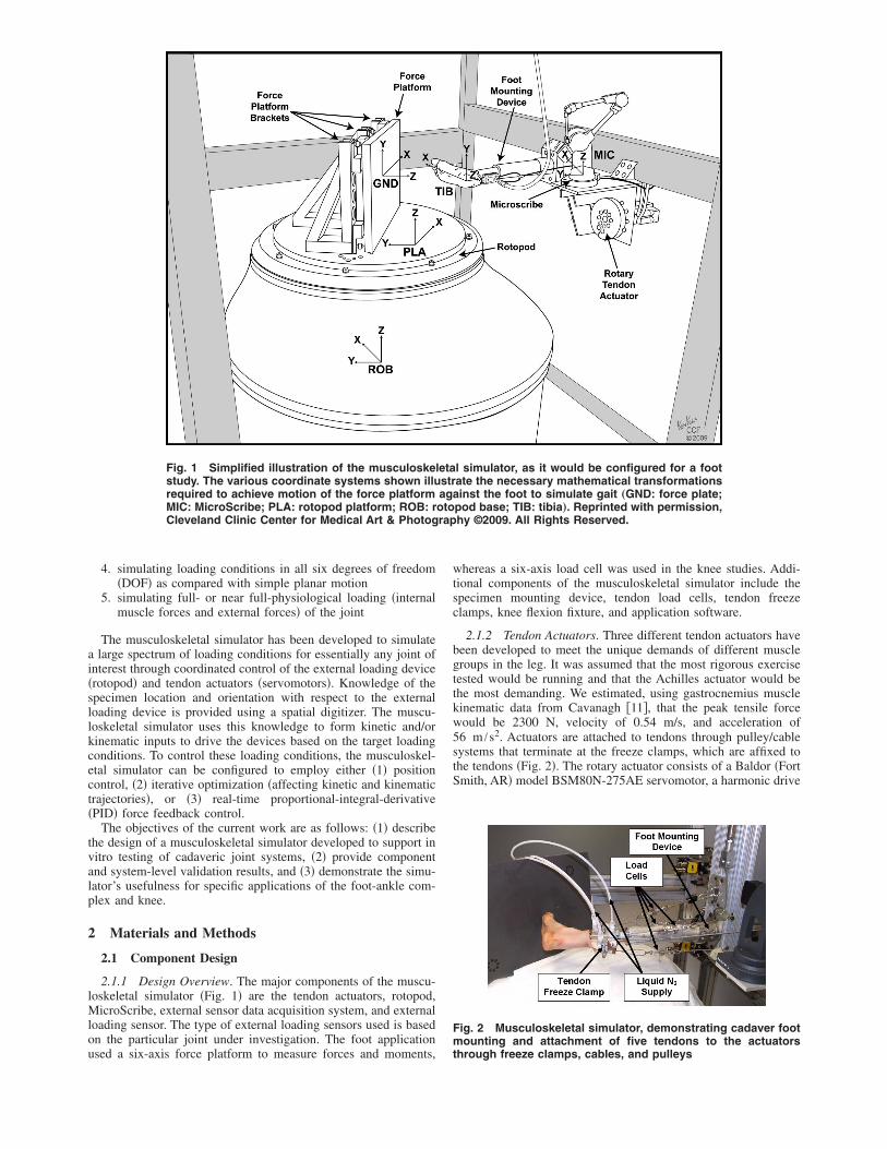
Fig. 1 Simplified illustration of the musculoskeletal simulator, as it would be configured for a foot study. The various coordinate systems shown illustrate the necessary mathematical transformations required to achieve motion of the force platform against the foot to simulate gait „GND: force plate; MIC: MicroScribe; PLA: rotopod platform; ROB: rotopod base; TIB: tibia…. Reprinted with permission, Cleveland Clinic Center for Medical Art & Photography ©2009. All Rights Reserved.

4. simulating loading conditions in all six degrees of freedom (DOF) as compared with simple planar motion

5. simulating full- or near full-physiological loading (internal muscle forces and external forces) of the joint

The musculoskeletal simulator has been developed to simulate a large spectrum of loading conditions for essentially any joint of interest through coordinated control of the external loading device (rotopod) and tendon actuators (servomotors). Knowledge of the specimen location and orientation with respect to the external loading device is provided using a spatial digitizer. The muscu­loskeletal simulator uses this knowledge to form kinetic and/or kinematic inputs to drive the devices based on the target loading conditions. To control these loading conditions, the musculoskel­etal simulator can be configured to employ either (1) position control, (2) iterative optimization (affecting kinetic and kinematic trajectories), or (3) real-time proportional-integral-derivative (PID) force feedback control.

The objectives of the current work are as follows: (1) describe the design of a musculoskeletal simulator developed to support in vitro testing of cadaveric joint systems, (2) provide component and system-level validation results, and (3) demonstrate the simu­lator’s usefulness for specific applications of the foot-ankle com­plex and knee.

2 Materials and Methods

2.1 Component Design

2.1.1 Design Overview. The major components of the muscu­loskeletal simulator (Fig. 1) are the tendon actuators, rotopod, MicroScribe, external sensor data acquisition system, and external loading sensor. The type of external loading sensors used is based on the particular joint under investigation. The foot application used a six-axis force platform to measure forces and moments,

whereas a six-axis load cell was used in the knee studies. Addi­tional components of the musculoskeletal simulator include the specimen mounting device, tendon load cells, tendon freeze clamps, knee flexion fixture, and application software.

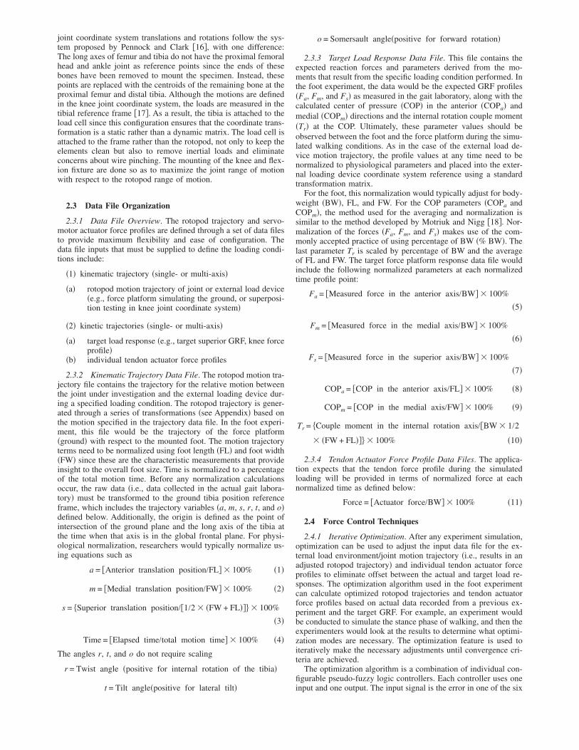
2.1.2 Tendon Actuators. Three different tendon actuators have been developed to meet the unique demands of different muscle groups in the leg. It was assumed that the most rigorous exercise tested would be running and that the Achilles actuator would be the most demanding. We estimated, using gastrocnemius muscle kinematic data from Cavanagh [11], that the peak tensile force would be 2300 N, velocity of 0.54 m/s, and acceleration of 56 m /s2. Actuators are attached to tendons through pulley/cable systems that terminate at the freeze clamps, which are affixed to the tendons (Fig. 2). The rotary actuator consists of a Baldor (Fort Smith, AR) model BSM80N-275AE servomotor, a harmonic drive

Fig. 2 Musculoskeletal simulator, demonstrating cadaver foot mounting and attachment of five tendons to the actuators through freeze clamps, cables, and pulleys

Table 1 Rotary tendon actuator characteristics Table 4 MicroScribe specifications

Feature Value

Drive reduction ratio 50:1 Peak static force (N) 6110 Continuous force (N) 1880 Maximum velocity (m/s) 0.40 Maximum acceleration (m /s2) 120

system (Hauppauge, NY) model CSG-40-50 harmonic drive, and a 175 mm diameter pulley (Table 1). This actuator was selected because it can exceed the force of the Achilles tendon during rigorous exercise. The velocity and acceleration capabilities of the actuator suggest that it can perform simulations of near real-time running. Since it incorporates a pulley system, there are practi­cally no limitations regarding tendon stroke, making this actuator suitable for simulating the action of many different musculoskel­etal systems. The linear actuators are Parker Hannifin Corp. (Cleveland, OH) ET50-Series electric actuators with SM233A ser­vomotors (Table 2). Two different varieties of linear actuators have been developed. One design provides a 50-mm stroke and the other a 100-mm stroke. The 50-mm stroke design was selected because the muscles used in the foot during walking would not exceed this range. The 100-mm stroke was selected for some fu­ture application that might need an extended stroke. The peak force is sufficient for the other muscles, and the velocity and acceleration parameters indicate that running simulations at half speeds are possible (note that acceleration scales by one-fourth when speed is scaled by one-half).

2.1.3 Rotopod. The R2000 rotopod, developed by Parallel Ro­botic Systems Corp. (Hampton, NH), is a 6DOF robot (Table 3). The rotopod is similar to a standard hexapod robot, but, due to the unique mounting configuration of the six actuators on a circular path, it is additionally capable of rotating a payload of ±720 deg about the Z-axis of the rotopod base coordinate system (ROB) (Fig. 1). The high load capacity of the rotopod makes it possible to provide full-physiological loading simulations, including run­ning loads [12]. However, the velocity capabilities suggest run-

Table 2 Linear tendon actuator characteristics

Feature Value

Peak static force (N) 1450 Continuous force (N) 560 Maximum velocity (m/s) 1.0 Maximum acceleration (m /s2) 14

Table 3 Rotopod specifications

Feature Value

Platform size (diameter) (mm) 780 Load capacity (N) 2000 Torque capacity (N m) 1000 Payload capacity (kg) 227 Translational velocity (mm/s) 100 Angular velocity (deg/s) 120 Static accuracy (fm) ±50 Repeatability (fm) 25 X-axis range of motion (mm) ±110 Y-axis range of motion (mm) ±110 Z-axis range of motion (mm) ±93 Roll range of motion (deg) ±13 Pitch range of motion (deg) +12, −19 Yaw range of motion (deg) ±720

Feature Value

Workspace (cm sphere) 168 Resolution (mm) 0.13 Accuracy (100 point ANSI sphere) (mm) 0.43

ANSI: American National Standards Institute.

ning simulations must be time scaled. The motion path and corre­sponding velocities required of the robot for simulating running will exceed the translational and rotational velocity capabilities of the robot. The repeatability and inherent high stiffness of this configuration are important for superposition testing methods.

2.1.4 MicroScribe. The MicroScribe G2L digitizer, developed by Immersion Corp. (San Jose, CA), provides spatial information on the rotopod, external load sensor, and the cadaver specimen for use by the application software. Once the relative locations of these components are determined, this software performs all three-dimensional transformations necessary to execute motion and calculates loading response in clinically relevant coordinate systems. One limitation of the MicroScribe (Table 4) is that the resolution and accuracy are not on the same order of magnitude as that of the rotopod. However, since the MicroScribe is used to define the relative coordinate systems of the musculoskeletal simulator components and the specimen, it must also be consid­ered that the variation and precision in determining anatomical references are much larger than the uncertainty in the Micro-Scribe. For these reasons, the software contains mitigation tech­niques such as optimization in the foot experiments and hybrid (force and position) control in the knee experiments.

2.1.5 External Sensor Data Acquisition System. The stand­alone data acquisition system is synchronized with the musculosk­eletal simulator, via the common digital synchronization bus and Ethernet, to provide up to 16 additional channels of analog data. Bone or soft tissue strain, joint pressure, or other analog voltage signals are acquired and conditioned using a National Instruments (Austin, TX) PCI-6229 data acquisition board and SCXI-1000 sig­nal conditioning chassis with a SCXI-1143 Butterworth 200 Hz low-pass, anti-aliasing filter.

2.1.6 Force Platform. A Bertec (Columbus, OH) force plate (model 4060) and amplifier (model 6800) were used for the foot experiments in combination with the National Instruments PCI­6034E data acquisition board for analog/digital conversion of the voltage analog outputs of forces (Fx, Fy, and Fz) and moments (Mx, My, and Mz). Characteristics of the force platform are pro­vided in Table 5.

2.1.7 Specimen Mounting Device. An aluminum tube that con­tains the potted specimen (foot, knee, etc.) slides into a receptacle device, where it is clamped into a stationary position during load­ing.

2.1.8 Tendon Freeze Clamps. Freeze clamps of two different sizes were developed at the Cleveland Clinic to attach the tendons to the tendon actuator cables. The bodies of these clamps allow the attachment of liquid nitrogen feed lines (Fig. 2).

2.1.9 Tendon Load Cells. Three Omega (Stamford, CT) LCFD-100 load cells (range: 0–445 N, accuracy: ±0.15% full scale, FS, repeatability: ±0.05% FS) and one LCFD-500 load cell (range: 0–2224 N, accuracy: ±0.2% FS, repeatability: ±0.1% FS) were used to measure the force of the individual tendons. Load cells were located in-line between the tendon freeze clamps and tendon actuator cables. In addition, one custom-made load cell incorporated into the pulley of the rotary tendon actuator, manu­

Table 5 Bertec force platform performance characteristics

Feature Value

Load rating Fx, Fy: 5000 N, Fz: 10,000 N Mx: 1500 N m, My: 1000 N m, Mz: 750 N m

Sensitivity Fx, Fy: 0.44 N/mV, Fz: 0.89 N/mV Mx: 0.27 N m/mV, My: 0.18 N m/mV, Mz: 0.13 N m/mV

Linearity ±2.0% FS Hysteresis ±2.0% FS Gain, selectable per channel 1, 2, 5 10, 20, 50, 100

factured by Strainsert (West Conshohocken, PA), is capable of measuring force in the range of 0–6720 N (accuracy: ±1% FS, repeatability: ±0.15% FS).

2.1.10 Six-Axis Load Cell. The ATI Industrial Automation (Apex, NC) Theta-series SI-1500-240 six-axis load cell (Table 6) was used during knee experiments to measure the loads observed at the tibia attributable to the rotopod. In this configuration, the tibia is purposely mounted in the inverted stationary position.

2.1.11 Knee Flexion Fixture. Given the range of motion of the rotopod, the musculoskeletal simulator is not able to explore the

full range of motion of the knee without an additional fixture to provide a seventh DOF. Although relatively small dynamic changes in flexion (about ±10 deg) are possible with the muscu­loskeletal simulator, the custom fixture illustrated in Fig. 3 allows for flexion of the knee from 0 deg to 120 deg.

2.1.12 Application Software. A software framework for the musculoskeletal simulator has been developed using National In­struments (Austin, TX) LabVIEW™ version 8.2. The framework was tested with both foot and knee applications. The system block diagram (Fig. 4) provides a general organization of application

Table 6 ATI Theta SI-1500-240 load cell performance characteristics

Value

Feature Fx Fy Fz Mx My Mz

Load rating (N, N m) 1500 1500 3750 240 240 240 Resolution (N, N m) 0.5 0.5 1.1 0.07 0.07 0.07 Accuracy (% FS) 1.50 1.25 0.75 1.25 1.00 1.50

Fig. 3 Simplified illustration of the musculoskeletal simulator, as it would be configured for a knee study. The various coordinate systems shown illustrate the necessary mathematical transformations required to achieve motion of the knee fixture to cause knee flexion „FEM: femur; FIX: knee flexion fixture; LOD: six-axis load cell; MIC: MicroScribe; PLA: rotopod platform; ROB: rotopod base…. Re­printed with permission, Cleveland Clinic Center for Medical Art & Photography ©2009. All Rights Reserved.

Fig. 4 Musculoskeletal simulator block diagram showing general components required for foot ex­periments. The synch bus allows synchronization between the rotopod, strain gauge data acquisi­tion, and tendon actuators during simulated gait „DOF, degrees of freedom…­

software required for the foot experiment. The external sensor data acquisition system software has been designed to run on a stand-alone workstation to handle the data acquisition processing, independent of the musculoskeletal simulator workstation proces­sor that provides the main application software. This architecture supports operation in master-slave configuration, by which the musculoskeletal simulator application software controls timing as­pects of the external sensor data acquisition system during the experiment.

A graphical user interface captures key aspects of the configu­ration and setup prior to execution of the experiment simulations. The application software provides the ability to interface with the MicroScribe to digitize the unique anatomical features of each specimen prior to testing to ensure that data are collected in a clinically relevant anatomical coordinate system. A flexible text­file-based system facilitates the input of muscle electromyogram data, kinematic data (motion analysis), and externally induced load data, such as would result from exercise. These input data are used to establish motion trajectories and tendon force profiles in the same clinically relevant coordinate systems as those used for the simulated exercises. During the experiment, the musculoskel­etal simulator software produces real-time graphs of engineering data retrieved through analog data input channels. For instance, displays of real-time force and moment data are provided in the tibial coordinate system during knee experiments.

2.2 Equipment Configuration

2.2.1 Foot Test Configuration. To conduct foot experiments, the musculoskeletal simulator uses kinetic trajectories (force pro­files) for the tendon actuators and for the target ground reaction forces (GRFs). The kinematic trajectory of the tibia relative to the ground, as measured in a gait laboratory, drives the rotopod mo­tion. The musculoskeletal simulator uses iterative optimization techniques to produce the target loading conditions, GRFs, and/or tendon actuators. The anatomical coordinate system is based on a proposed International Society of Biomechanics standard [13].

However, because of the unique nature of cadaveric simulators, a custom reference frame was defined as the tibial coordinate sys­tem (TIB). Since the TIB defines the ankle center and is used to orient GRF and ground tibia position data, one needs to consider the orientation of the tibia as well as the foot. Like the knee joint, variations from the standard coordinate system account for miss­ing anatomical reference points caused by the cutting and mount­ing of limbs. The tibial intercondylar point is replaced with the centroid of the tibia measured at the most proximal location pos­sible, and to increase repeatability of the specimen coordinate system, the mediolateral axis is redefined as an axis perpendicular to the midline of the foot [14]. For orientation of the tibia relative to the ground, Yeadon’s [15] “somersault-tilt-twist” variables are used. The Yeadon rotation sequence twist (which is renamed as internal rotation) is measured about the tibial long axis; somer­sault is measured about the global mediolateral axis. To recreate typical foot-ankle motion, the tibia is fixed horizontally on the surrounding frame, and the force plate is mounted vertically on the top of the rotopod platform to create an inverted ground-tibia motion (Fig. 1). This method provides two major benefits. First, it does not require moving the entire tendon actuator system along with the tibia motion during a simulation. Second, the largest foot-ankle rotation (somersault) can be adequately simulated be­cause of the rotopod’s unique ability to provide large rotations in the horizontal plane. One limitation of this configuration is that the inertial loading of the specimen cannot fully be replicated because of the quasi-static nature of the simulations; we compen­sate for this factor by slight changes in rotopod motion via the optimization process.

2.2.2 Knee Test Configuration. The musculoskeletal simulator, configured to conduct knee experiments, can operate in position or force control. Given a kinematic input file, the musculoskeletal simulator can step through the motion sequence and store data at each position. Given a kinetic input file, the musculoskeletal simulator can ramp to each loading condition via a real-time hy­brid controller (simultaneous position and force control). The knee

joint coordinate system translations and rotations follow the sys­tem proposed by Pennock and Clark [16], with one difference: The long axes of femur and tibia do not have the proximal femoral head and ankle joint as reference points since the ends of these bones have been removed to mount the specimen. Instead, these points are replaced with the centroids of the remaining bone at the proximal femur and distal tibia. Although the motions are defined in the knee joint coordinate system, the loads are measured in the tibial reference frame [17]. As a result, the tibia is attached to the load cell since this configuration ensures that the coordinate trans­formation is a static rather than a dynamic matrix. The load cell is attached to the frame rather than the rotopod, not only to keep the elements clean but also to remove inertial loads and eliminate concerns about wire pinching. The mounting of the knee and flex­ion fixture are done so as to maximize the joint range of motion with respect to the rotopod range of motion.

2.3 Data File Organization

2.3.1 Data File Overview. The rotopod trajectory and servo­motor actuator force profiles are defined through a set of data files to provide maximum flexibility and ease of configuration. The data file inputs that must be supplied to define the loading condi­tions include:

(1) kinematic trajectory (single- or multi-axis)

(a) rotopod motion trajectory of joint or external load device (e.g., force platform simulating the ground, or superposi­tion testing in knee joint coordinate system)

(2) kinetic trajectories (single- or multi-axis)

(a) target load response (e.g., target superior GRF, knee force profile)

(b) individual tendon actuator force profiles

2.3.2 Kinematic Trajectory Data File. The rotopod motion tra­jectory file contains the trajectory for the relative motion between the joint under investigation and the external loading device dur­ing a specified loading condition. The rotopod trajectory is gener­ated through a series of transformations (see Appendix) based on the motion specified in the trajectory data file. In the foot experi­ment, this file would be the trajectory of the force platform (ground) with respect to the mounted foot. The motion trajectory terms need to be normalized using foot length (FL) and foot width (FW) since these are the characteristic measurements that provide insight to the overall foot size. Time is normalized to a percentage of the total motion time. Before any normalization calculations occur, the raw data (i.e., data collected in the actual gait labora­tory) must be transformed to the ground tibia position reference frame, which includes the trajectory variables (a, m, s, r, t, and o) defined below. Additionally, the origin is defined as the point of intersection of the ground plane and the long axis of the tibia at the time when that axis is in the global frontal plane. For physi­ological normalization, researchers would typically normalize us­ing equations such as

a = [Anterior translation position/FL] X 100% (1)

m = [Medial translation position/FW] X 100% (2)

s = {Superior translation position/[1/2 X (FW + FL)]} X 100%

(3)

Time = [Elapsed time/total motion time] X 100% (4)

The angles r, t, and o do not require scaling

r = Twist angle (positive for internal rotation of the tibia)

t = Tilt angle(positive for lateral tilt)

o = Somersault angle(positive for forward rotation)

2.3.3 Target Load Response Data File. This file contains the expected reaction forces and parameters derived from the mo­ments that result from the specific loading condition performed. In the foot experiment, the data would be the expected GRF profiles (Fa, Fm, and Fs) as measured in the gait laboratory, along with the calculated center of pressure (COP) in the anterior (COPa) and medial (COPm) directions and the internal rotation couple moment (Tr) at the COP. Ultimately, these parameter values should be observed between the foot and the force platform during the simu­lated walking conditions. As in the case of the external load de­vice motion trajectory, the profile values at any time need to be normalized to physiological parameters and placed into the exter­nal loading device coordinate system reference using a standard transformation matrix.

For the foot, this normalization would typically adjust for body-weight (BW), FL, and FW. For the COP parameters (COPa and COPm), the method used for the averaging and normalization is similar to the method developed by Motriuk and Nigg [18]. Nor­malization of the forces (Fa, Fm, and Fs) makes use of the com­monly accepted practice of using percentage of BW (% BW). The last parameter Tr is scaled by percentage of BW and the average of FL and FW. The target force platform response data file would include the following normalized parameters at each normalized time profile point:

Fa = [Measured force in the anterior axis/BW] X 100%

(5)

Fm = [Measured force in the medial axis/BW] X 100%

(6)

Fs = [Measured force in the superior axis/BW] X 100%

(7)

COPa = [COP in the anterior axis/FL] X 100% (8)

COPm = [COP in the medial axis/FW] X 100% (9)

Tr = {Couple moment in the internal rotation axis/[BW X 1/2

X (FW + FL)]} X 100% (10)

2.3.4 Tendon Actuator Force Profile Data Files. The applica­tion expects that the tendon force profile during the simulated loading will be provided in terms of normalized force at each normalized time as defined below:

Force = [Actuator force/BW] X 100% (11)

2.4 Force Control Techniques

2.4.1 Iterative Optimization. After any experiment simulation, optimization can be used to adjust the input data file for the ex­ternal load environment/joint motion trajectory (i.e., results in an adjusted rotopod trajectory) and individual tendon actuator force profiles to eliminate offset between the actual and target load re­sponses. The optimization algorithm used in the foot experiment can calculate optimized rotopod trajectories and tendon actuator force profiles based on actual data recorded from a previous ex­periment and the target GRF. For example, an experiment would be conducted to simulate the stance phase of walking, and then the experimenters would look at the results to determine what optimi­zation modes are necessary. The optimization feature is used to iteratively make the necessary adjustments until convergence cri­teria are achieved.

The optimization algorithm is a combination of individual con­figurable pseudo-fuzzy logic controllers. Each controller uses one input and one output. The input signal is the error in one of the six

GRF channels, and the output signal is then added to the chosen simulator channel (e.g., superior motion, tibialis anterior force, etc.). The controller processes the input by selective windowing (% stance range within which data are to be analyzed), applying the chosen algorithm (i.e., use mean, absolute value, or point-by­point), low-pass filtering, multiplying by a gain parameter, and finally adding to the output channel data from the previous run to produce the optimized output signal for that same channel. Mul­tiple controllers acting on the same simulator channel are collec­tively summed to produce the optimized trajectories used for the subsequent test.

Optimization of muscle forces is considered to be adaptive such that the viscoelastic response of the tendon from the previous experiment is taken into consideration when making adjustments for the subsequent experiment. For instance, if the superior GRF (Fs) did not achieve the target peak value at toe-off (e.g., the triceps surae muscle group did not reach the target tension at that time), then optimization can increase the force to this muscle group at that same time by an amount equal to the following:

Ftriceps surae(new) = Ftriceps surae(previous) + Gain X (Fs target

− Fs actual) (12)

Similarly, optimization provides the flexibility necessary to adjust for positional misalignment between the joint coordinate system and device contacting the joint to provide loading. To illustrate this possibility, consider the origin of the tibia coordinate system X, Y, and Z in the ankle (identified as TIB in Fig. 1). If the actual origin were 1 mm in the Z-direction from what was recorded with the MicroScribe during set up of the experiment, then it would manifest itself as low Fs during the experiment, and optimization can be invoked to adjust for this discrepancy. The result would be to shift the force platform trajectory by a constant amount in the Z-direction for all time increments during simulated stance, such that the Z-position (new) is now computed as

Z-position(new) = Z-position(previous) + Gain X Mean(Fs target

− Fs actual) (13)

In this case, the mean value is computed for the difference in Fs across all time increments. This mean is then multiplied by a constant gain value to achieve the Z-value offset for the force platform trajectory.

2.4.2 Real-Time Hybrid Control. In the knee experiments, the aim is to provide simultaneous position and force control. The flexion axis of the knee has very little stiffness, and controlling moment about that axis would be unlikely to provide a unique solution. For this reason, the joint is controlled in three axes of force control (anterior, medial, and superior), two axes of torque control (varus and internal rotations), and one axis of angle con­trol (flexion). This PID hybrid control scheme operates in a varia­tion in the knee joint coordinate system to maximize decoupling. The controller transforms the data from the load cell coordinate system to the tibial coordinate system [19]. Then superior force and varus torque are decoupled into two superior forces, each located at the center of each femoral condyle. Following the PID algorithm, the resulting command signals are integrated with re­spect to time, recoupled to the knee joint coordinate system, and transformed to the rotopod coordinate system. In addition, the hybrid controller employs other tools, such as gain scheduling and feed forward, to further enhance speed and stability.

2.5 Validation Methods. Validation of this complex system included evaluating the general capabilities of the major compo­nents (subsystems) as well as demonstrating the performance of the full system when configured to conduct foot and knee experi­ments.

2.5.1 Tendon Actuator Accuracy and Repeatability Validation Tests. A foot study designed to simulate gait was used to test the mean absolute accuracy and repeatability of the tendon actuators at achieving the target tendon force levels. Six experiments con­ducted on two specimens provided data from multiple experi­ments at the same loading conditions. Absolute errors were com­puted between actual and target force at each time interval during stance for each experiment and reported as a mean ±1 standard deviation. Repeatability was visualized by plotting the target force against the actual force for various experiments for periods of simulated muscle contractions. Simulated relaxation was not in­cluded in the plots because hysteresis that results between con­traction and relaxation further complicates the plots (i.e., two points per experiment at each stance point).

2.5.2 Component Synchronization Validation Tests. To syn­chronize the entire system, the low-level programs of the rotopod and tendon actuators, and the internal and external data acquisi­tion systems were coded to start their respective processes at the moment when the rotopod’s controller generates a digital falling trigger signal. Since the external data acquisition system was coded to poll the digital trigger signal every 1 ms, the timing delay between the digital trigger signal and the external data was a maximum of 1 ms. The internal data acquisition system pre-acquires data and is postprocessed to align to the trigger, resulting in a delay, which is also -1 ms. The timing delay of the me­chanical components’ motion from the digital trigger signal was evaluated by performing a step functionlike motion profile. Ten tests each were conducted on the rotopod, rotary tendon actuator, and linear tendon actuators to measure the motion delay from the start of the synchronization trigger signal. System synchronization accuracy can be estimated by the following equation:

Synchronization system accuracy

Max. delay + Min. delay Max. delay − Min. delay =

2 ±

2

(14)

2.5.3 Rotopod Position Accuracy Validation Test. The rotopod provides motion, force input, or both to the joint of interest. The control of force is done through real-time feedback control, as in the knee experiments, or iterative force control, as in the foot experiments. Fundamentally, position is iterated to reach the target force. Therefore, a series of tests were run to determine the quasi-static and dynamic translational accuracy of the rotopod when loaded (with a payload of 98.2 kg) and unloaded. The quasi-static test motion path was a stepped triangle wave (10 mm per step) over the full range of motion (±100 mm in each axis), quantifying uniaxial position error. The dynamic test path was a 0.167 Hz sinusoidal waveform corresponding to a peak speed of 100 mm/s (maximum capability of the rotopod) for the same range of mo­tion. A Heidenhain Corp. (Shaumburg, IL) model LS679 linear encoder, having an accuracy of 10 fm and a resolution of 0.5 fm, was used to measure the movement of the robot. Accu­racy was assessed by maximum (max) and root-mean-square (rms) positional errors for the full range of motion (similar to the foot experiment) and for the center range of motion (±30 mm, as in the knee experiment).

2.5.4 Optimization Validation Test. Experiment optimization was invoked to target the heel strike and the latter half of stance during foot experiments to achieve reasonable simulated walking. This capability was tested through a series of seven experiments: Experiments 1–4 focused on adjusting offsets during heel strike, whereas experiments 5–7 focused on adjusting the muscle forces from midstance through toe-off.

2.5.5 Foot Test Demonstration. The foot experiment configu­ration of the musculoskeletal simulator has been used to measure various biomechanical parameters in studies of normal and patho­

Fig. 5 Tendon actuator accuracy results for two experiments of three runs each, in which under closed-loop feedback, the actuator of the musculoskeletal simulator simulates muscle contractions. Muscles included „a… triceps surae, „b… tibialis anterior, „c… tibialis posterior, „d… peroneus longus, and „e… flexor hallucis longus. Note that absolute error is shown as a mean ±1 standard deviation. Target force is included as a reference.

logical gaits. In a recent study [20], it was used to investigate the effects of diabetes on the midfoot joint pressures. A foot study designed to acquire tibial and calcaneal bone strain data during simulating gait is used to demonstrate the musculoskeletal simu­lator capabilities in a foot experiment configuration. Tibial and calcaneal strain data were collected using Vishay Micro-Measurements (Raleigh, NC) rosette C2A-06-031WW-120. Test­ing was performed to verify that analog data (in this case, strain data) could be synchronized through the digital synchronization bus and collected during the entire stance phase of simulated walking in a reliable and repeatable manner. Two 2100 system signal conditioning amplifiers (Vishay Micro-Measurements) were used to provide quarter-bridge circuit conditioning and am­plification required for these strain gauge rosettes. The locations of these rosettes were anterior tibia (lateral and medial sides), posterior tibia, and lateral calcaneus for a total of 12 channels of raw strain data. The foot study simulated walking at one-fourth speed and varying BW percentages (16.5%, 38.4%, 66.7%, and 100% BW). Graphs of the target and actual GRF data, along with the tendon force data, for a representative experiment are pre­sented.

2.5.6 Knee Test Demonstration. The musculoskeletal simula­tor has been used to study native kinematics, arthroplasty, and surgical techniques in the knee joint. In one study, the knee test

system was programmed to apply 108 combinations of the follow­ing loading conditions at three flexion angles (0 deg, 30 deg, and 60 deg): internal/external rotation (0 N m, ±5 N m), varus/valgus (0 N m, ±10 N m), compression (100 N, 700 N), and posterior drawer (0 N, 100 N). The combined loading condition was ramped, held, and released in 2 s, 3 s, and 1 s, respectively. The error between the target and actual forces, or torques, is analyzed continuously as well as during the plateau (at which point auxil­iary data is typically collected).

3 Results

3.1 Tendon Actuator Accuracy and Repeatability Results. Tests conducted to measure the error between target and actual tendon actuator forces revealed a large variability in absolute error (which was dependent on the stance time; Fig. 5), but these tests demonstrated that within multiple runs of the same experiment there was excellent repeatability (Fig. 6).

3.2 Component Synchronization Results. Test results of synchronization revealed that the rotopod contributes the largest delay at 10.8±1.0 ms, followed by the linear actuator at 5.2± 1.4 ms, then the rotary actuator at 4.1±1.0 ms. Using Eq. (14), the total synchronization system accuracy was 6.7±2.0 ms.

Fig. 6 Tendon actuator repeatability results for two experiments of three runs each, in which under closed-loop feedback, the actuator of the musculoskeletal simulator simulates muscle contractions. Muscles included „a… triceps surae, „b… tibialis anterior, „c… tibialis posterior, „d… peroneus longus, and „e… flexor hallucis longus. Note that relative accuracy can be seen in deviation from the theoretical line.

3.3 Rotopod Positioning Results. The rotopod positioning tact by changing the anterior and superior coordinates of the tibial test results (Table 7) ranged from 10 fm to 359 fm, depending coordinate system. Table 8 summarizes what changes were made on measurement condition. The Z-axis position error is roughly 2 for the first four experiments to simulate heel strike. Experiments times the error for the X- and Y-axes. In general, loaded errors 5–7 used time-based adjustments to the plantarflexors (triceps were higher than the unloaded errors by 1.2, 1.3, and 1.6 times, surae, flexor hallucis, tibialis posterior, and peroneus longus) to for the X-, Y-, and Z-axis, respectively. bring the superior GRF to within ±10% of the target force during

loading response, midstance, terminal stance, and toe-off contact 3.4 Optimization Results. A typical optimization scenario is phases.

depicted in Fig. 7. Experiments 1–4 were used to adjust the supe­rior GRF to achieve the target level at the initial heel strike con- 3.5 Foot Test Demonstration. The optimization target of

Table 7 Rotopod positioning results

X-axis Y-axis Z-axis

Position error (fm) Unloaded Loaded Unloaded Loaded Unloaded Loaded

Quasi-static full (max) 56 99 37 50 74 234 Quasi-static full (rms) 24 28 18 29 36 84 Quasi-static center (max) 55 27 32 44 58 61 Quasi-static center (rms) 26 16 19 24 33 30 Dynamic full (max) 89 108 79 127 206 359 Dynamic full (rms) 31 38 30 31 63 110 Dynamic center (max) 27 39 62 58 95 85 Dynamic center (rms) 10 15 26 19 52 49

Max: maximum; rms: root-mean-square.

Fig. 7 Optimization results for seven experiments, showing convergence of superior force against the target toe-off region profile during simulated gait using the musculoskeletal simulator.

±10% was achieved at heel strike and toe-off in the superior axis during simulated gait using the musculoskeletal simulator (Fig. 8). In the anterior and COP channels, the goal was to optimize the kinetic and kinematic trajectories to the point where the target and actual curves had a similar form. For this experiment, further op­timization to better achieve the target profiles was not necessary to obtain the desired bone strain results.

3.6 Knee Test Demonstration. The hybrid controller demon­strated that low errors can be achieved on the superior compres­sion channel during the course of the 108 combined loading con­ditions (see Fig. 9 for a representative graph). The highest errors (rms and max) were found to be in the continuous comparison analysis (Table 9).

4 Discussion

4.1 Tendon Actuator Accuracy and Repeatability. Force accuracy results achieved with the tendon actuators during the

Table 8 Optimization during heel strike

Anterior Superior Experiment offset offset

No. (mm) (mm) Summary of results

1 0 -13 Starting point; no heel contact with force platform 2 4 -11 Force platform contacted the heel 4 mm forward (anterior direction)

of the initial run and moved 2 mm closer (superior direction) to the bottom of the foot. This achieved 36% BW (target 44% BW).

3 5 -10.5 Force platform trajectory was adjusted another 1 mm and closer to the mounted foot by 0.5 mm. This achieved 43% BW.

4 9.5 -10.5 Force platform trajectory was adjusted 4.5 mm forward (anteriorly) from previous run with no change in the proximity to the foot (superior direction) at the start. This had an adverse affect by overshooting to 47% BW. Note: The previous iteration’s anterior offset (5 mm) was ultimately used for the final experiment settings.

Fig. 8 Selected results from the foot bone strain study using the musculoskeletal simulator are shown. Full-physiological loading is demonstrated through „a… the superior and „b… anterior ground reaction forces, „c… anterior center of pressure, and „d… muscle forces. Results shown are indicative of a typical experiment run.

Fig. 9 Representative superior compression force profile of the real-time proportional-integral-derivative „PID… hybrid con­trol for a knee experiment using the musculoskeletal simulator.

musculoskeletal simulator performance verification process were sufficient to accurately simulate gait for the foot bone strain study. The ability of the tendon actuators to achieve the target muscle force profile is dependent on the resolution of the in-line load cells and controller gains (PID). The load cell resolution was found to correlate (R2=0.85) with the tendon actuator accuracy. The load cell used with the actuator simulating the tibialis posterior muscle had a resolution of 0.54 N per count (12 bit analog/digital con­verter counts), the load cell used with the triceps surae actuator had a resolution of 0.19 N per count, and the remaining load cells had resolutions of 0.10 N per count. Excellent repeatability results were demonstrated for the tendon actuators, with an average error of 0.3% BW. Tendon actuator accuracy posed no limitations to the particular foot study; therefore, no further optimization was deemed necessary. A one-time adjustment was made to the con­troller PID gains, velocity parameters, and acceleration param­eters for the linear tendon actuators. This adjustment resulted in a substantial performance improvement, which was sufficient for the foot study. Future studies that require an even higher level of accuracy may achieve it by optimization of these parameters.

4.2 Component Synchronization. Provided that the duration of the activity being simulated is significantly larger than the syn­chronization error (6.7± 2.0 ms), the effect of the error will be insignificant for future researchers. For the foot study presented, the simulated walking motion was 2.8 s. Therefore, this error rep­resents 0.24% of the total experiment time and is not considered significant.

4.3 Rotopod Positioning Discussion. The highest error val­ues measured were for Z-axis motion, potentially due to consid­erable changes in the configuration of the robot legs. Loading generally increased error magnitude but was not pronounced for the center range of motion. The error values were less than those found in other studies, [10] and therefore, are adequate for in vitro reproduction of certain motions.

4.4 Optimization. A typical optimization procedure was dis­cussed, showing that the system has the necessary flexibility to

successfully optimize the trajectory (required for heel strike ad­justment) and for muscle force optimization (required for the lat­ter phase of stance). During the foot study, it was found that typically within 3–6 iterations of trajectory optimization, it was possible to obtain a heel strike force within the target limit of ±10% of the target superior GRF. Similarly, within 4–8 iterations of muscle force optimization, the latter half of stance was within this limit. Optimization adjusted the target muscle forces by an amount proportional to the measured parameter (superior force error); therefore, subsequent iterations of optimization converged on acceptable muscle forces regardless of whether or not they matched the target force set point. Stability of the optimization algorithm is therefore much more dependent on repeatability of the actuators and the rotopod, which has been shown to be very high. Although the fuzzy logic controllers were effective on this experiment, one limitation is that the algorithms provided nonu­nique solutions to the optimization, given that there were six in­puts (GRF) and 11 outputs (6DOF kinematics and five tendon actuators). Future enhancement of the optimization algorithm may be necessary, depending on the requirements for a given study. To provide for this possibility, the musculoskeletal simulator software can be customized within the existing software framework to al­low the implementation of fuzzy logic, model predictive, linear optimization, or any other control philosophy.

4.5 Foot and Knee Test Demonstrations. Through the completion of the performance validation process, several key features of the musculoskeletal simulator have been demonstrated. Multiple joints have undergone 6DOF simulations at full-physiological loading conditions. Full-physiological loadings of the foot and knee were achieved with the musculoskeletal simu­lator in a stable and highly repeatable manner.

Foot experiments used programmable loading conditions and operated at one-fourth walking speed. Synchronization of system components, accuracy of tendon actuators and of rotopod position, and the results of the foot experiment systematically demonstrate that the musculoskeletal simulator is able to simulate an entire gait cycle through coordinated motion of the rotopod and tendon ac­tuators while simultaneously recording 12 channels of bone strain.

In the knee experiment, one limitation to achieving the dynamic motion demonstrated by the foot experiment is the static adjust-ability of the flexion fixture. As a result of this limitation, tests had to be paused in order to manually adjust the fixture to provide greater changes in knee flexion. Work has recently been com­pleted to remove this constraint by developing a rotary stage mounted on top of the rotopod. This stage provides dynamic flex­ion capabilities for knee, shoulder, and hip experiments with a range of ±180 deg.

The representative errors in the real-time hybrid control are minimal in the plateau measurements and sufficient for testing where quasi-static combinations of loads are applied. Figure 9 suggests that the continuous errors in Table 9 result from the inherent lag in PID control algorithms. In studies for which real-time dynamic loading is desired, improvements would need to be made in the response time of the control system by modifying this algorithm or implementing a new one.

Table 9 Representative knee force/torque control errors

Value

Force/torque control error Flateral (N)

Fanterior (N)

Fsuperior(N)

TVarus (N m)

TER (N m)

Plateau (max) 1 3 10 0.1 0.2 Plateau (rms) <1 1 4 0.04 0.1 Continuous (max) 73 69 330 9.4 1.4 Continuous (rms) 11 16 71 1.3 0.3

TER: torque, external rotation; max: maximum; rms: root-mean-square.

5 Conclusions

The musculoskeletal simulator has been shown to simulate the biomechanics of human motion through (i) a set of actuators that, when connected to selected tendons traversing a joint, can imitate muscular contractions, and (ii) a rotopod that can simulate envi­ronmentally induced loading of and contact with the cadaver specimen. The benefit of these coupled systems is that they enable fully synchronized joint loading at physiological levels, at or near real-time speeds. The design of the musculoskeletal simulator makes it readily adaptable for investigation of many different joint systems. The musculoskeletal simulator has been developed to enable fundamental research that is focused on injury prevention, but the applications extend into other areas such as the evaluation of surgical interventions and total joint replacements and the de­velopment of rehabilitation regimens.

Acknowledgment The authors would like to acknowledge the support for this

research from NASA Grant No. NNJ05HF55G and from the Cleveland Clinic Musculoskeletal Core Center, funded in part by NIAMS Core Center Grant No. 1P30 AR-050953. In addition, the efforts of Katherine Muterspaugh in providing LabVIEW routines for sampling and storing bone strain data are appreciated. Special thanks to Ken Kula (Cleveland Clinic Center for Medical Art and Photography) for providing the artist renditions of the Musculosk­eletal Simulator. Finally, the support of the Cleveland Clinic is gratefully acknowledged through the contributions of Peter R. Ca­vanagh, Ph.D., D.Sc. (now of the University of Washington/ Seattle) for providing the rotopod and Ahmet Erdemir, Ph.D., from the Computational Biomodeling Core, for providing rotopod test results.

Appendix: Transformation of Three-Dimensional Kine­matic Data to Rotopod Trajectory (Foot and Knee Ex­amples)

This appendix illustrates the kinematic chain equation, as shown in Eqs. (15) and (16), for typical foot and knee experi­ments, respectively. The expressions include reference frames for the rotopod base (ROB), the rotopod platform (PLA), the force plate (GND), the knee flexion fixture (FIX), the six-axis load cell (LOD), the MicroScribe (MIC), the tibia (TIB), and the femur (FEM). The static transformation matrices for the foot are TROB,MIC, TPLA,GND, and TTIB,MIC. The corresponding dynamic matrices are TROB,PLA and TGND,TIB. The static transformation matrices for the knee are TROB,MIC, TTIB,MIC, and the configurable TPLA,FIX. The corresponding dynamic matrices are TROB,PLA and TFEM,TIB. These equations can be used to derive the elements of any one dynamic matrix given the other dynamic matrix (such as deriving rotopod positions given the motion of the tibia relative to the ground) that may have been collected in a gait laboratory setting. Refer to Figs. 1 and 3 for the location of each reference frame.

TROB,MIC = TROB,PLA(q) · TPLA,GND · TGND,TBD · TTIB,MIC(r) (15)

TROB,MIC = TROB,PLA(q) · TPLA,FIX(8) · TFIX,FEM

· TFEM,TIB(KJCS) · TTIB,MIC

where the rotopod coordinates are as follows:

(16)

q = (x,y,z,roll,pitch,yaw) the ground/tibia position are as follows:

r = (a,m,s,r,t,o) the flexion fixture setting are as follows:

8 = Nominal knee flexion angle

the knee joint coordinates [16,21] are as follows:

KJCS = (a,b,c,a,[,y)

References [1] Lanyon, L. E., Hampson, W. G., Goodship, A. E., and Shah, J. S., 1975, “Bone

Deformation Recorded In Vivo From Strain Gauges Attached to the Human Tibial Shaft,” Acta Orthop. Scand., 46, pp. 256–268.

[2] Burr, D. B., Milgrom, C., Fyhrie, D., Forwood, M., Nyska, M., Finestone, A., Hoshaw, S., Saiag, E., and Simkin, A., 1996, “In Vivo Measurement of Human Tibial Strains during Vigorous Activity,” Bone (N.Y.), 18, pp. 405–410.

[3] Weiss, J. A., Gardiner, J. C., Ellis, B. J., Lujan, T. J., and Phatak, N. S., 2005, “Three-Dimensional Finite Element Modeling of Ligaments: Technical As­pects,” Med. Eng. Phys., 27, pp. 845–861.

[4] Sharkey, N. A., and Hamel, A. J., 1998, “A Dynamic Cadaver Model of the Stance Phase of Gait: Performance Characteristics and Kinetic Validation,” Clin. Biomech. (Bristol, Avon), 13, pp. 420–433.

[5] Milgrom, C., Finestone, A., Hamel, A., Mandes, V., Burr, D., and Sharkey, N., 2004, “A Comparison of Bone Strain Measurements at Anatomically Relevant Sites Using Surface Gauges Versus Strain Gauged Bone Staples,” J. Biomech., 37, pp. 947–952.

[6] Hurschler, C., Emmerich, J., and Wülker, N., 2003, “In Vitro Simulation of Stance Phase Gait—Part I: Model Verification,” Foot Ankle Int., 24, pp. 614– 622.

[7] Kim, K.-J., Kitaoka, H. B., Luo, Z.-P., Ozeki, S., Berglund, L. J., Kaufman, K. R., and An, K.-N., 2001, “In Vitro Simulation of the Stance Phase in Human Gait,” Journal of Musculoskeletal Research, 5, pp. 113–121.

[8] Kim, K. J., Uchiyama, E., Kitaoka, H. B., and An, K. N., 2003, “An In Vitro Study of Individual Ankle Muscle Actions on the Center of Pressure,” Gait Posture, 17, pp. 125–131.

[9] Ward, E. D., Smith, K. M., Cocheba, J. R., Patterson, P. E., and Phillips, R. D., 2003, “In Vivo Forces in the Plantar Fascia During the Stance Phase of Gait: Sequential Release of the Plantar Fascia,” J. Am. Podiatr. Med. Assoc., 93, pp. 429–442.

[10] Howard, R. A., Rosvold, J. M., Darcy, S. P., Corr, D. T., Shrive, N. G., Tapper, J. E., Ronsky, J. L., Beveridge, J. E., Marchuk, L. L., and Frank, C. B., 2007, “Reproduction of In Vivo Motion Using a Parallel Robot,” ASME J. Biomech. Eng., 129, pp. 743–749.

[11] Cavanagh, P. R., ed., 1990, Biomechanics of Distance Running, Human Kinet­ics Publishers, Champaign, IL, pp. 92–93.

[12] Riley, P. O., Dicharry, J., Franz, J., Croce, U. D., Wilder, R. P., and Kerrigan, D. C., 2008, “A Kinematics and Kinetic Comparison of Overground and Treadmill Running,” Med. Sci. Sports Exercise, 40, pp. 1093–1100.

[13] Wu, G., Siegler, S., Allard, P., Kirtley, C., Leardini, A., Rosenbaum, D., Whittle, M., D’Lima, D. D., Cristofolini, L., Witte, H., Schmid, O., Stokes, I., and Standardization and Terminology Committee of the International Society of Biomechanics, 2002, “ISB Recommendation on Definitions of Joint Coor­dinate System of Various Joints for the Reporting of Human Joint Motion— Part I: Ankle, Hip, and Spine,” J. Biomech., 35, pp. 543–548.

[14] Isman, R. E., and Inman, V. T., 1969, “Anthropometric Studies of the Human Foot and Ankle,” Bull. Prosthet. Res., 11, pp. 97–129.

[15] Yeadon, M. R., 1990, “The Simulation of Aerial Movement—I. The Determi­nation of Orientation Angles From Film Data,” J. Biomech., 23, pp. 59–66.

[16] Pennock, G. R., and Clark, K. J., 1990, “An Anatomy-Based Coordinate Sys­tem for the Description of the Kinematic Displacements in the Human Knee,” J. Biomech., 23, pp. 1209–1218.

[17] Woo, S. L., Kanamori, A., Zeminski, J., Yagi, M., Papageorgiou, C., and Fu, F. H., 2002, “The Effectiveness of Reconstruction of the Anterior Cruciate Liga­ment With Hamstrings and Patellar Tendon. A Cadaveric Study Comparing Anterior Tibial and Rotational Loads,” J. Bone Jt. Surg., Am. Vol., 84-A, pp. 907–914.

[18] Motriuk, H. U., and Nigg, B. M., 1990, “A Technique for Normalizing Centre of Pressure Paths,” J. Biomech., 23, pp. 927–932.

[19] Fujie, H., Livesay, G. A., Woo, S. L., Kashiwaguchi, S., and Blomstrom, G., 1995, “The Use of a Universal Force-Moment Sensor to Determine In-Situ Forces in Ligaments: A New Methodology,” ASME J. Biomech. Eng., 117, pp. 1–7.

[20] Lee, D. G., and Davis, B. L., 2009, “Assessment of the Effects of Diabetes on Midfott Joint Pressure Using a Robotic Gait Simulator,” Foot Ankle Int., 30, pp. 767–772.

[21] Grood, E. S., and Suntay, W. J., 1983, “A Joint Coordinate System for the Clinical Description of Three-Dimensional Motions: Application to the Knee,” ASME J. Biomech. Eng., 105, pp. 136–144.