design and use of linear models for image motion analysisjepson/papers/fleetblackyacoob... ·...

International Journal of Computer Vision 36(3), 171–193, 2000c© 2000 Kluwer Academic Publishers. Manufactured in The Netherlands.

Design and Use of Linear Models for Image Motion Analysis

DAVID J. FLEETDepartment of Computing and Information Science, Queen’s University, Kingston, Ontario, Canada, K7L 3N6;

Xerox Palo Alto Research Center, 3333 Coyote Hill Road, Palo Alto, CA 94304, [email protected]

MICHAEL J. BLACKXerox Palo Alto Research Center, 3333 Coyote Hill Road, Palo Alto, CA 94304, USA

[email protected]

YASER YACOOBComputer Vision Laboratory, University of Maryland, College Park, MD 20742, USA

[email protected]

ALLAN D. JEPSONDepartment of Computer Science, University of Toronto, Toronto, Ontario, Canada, M5S 1A4

[email protected]

Received April 4, 1999; Revised December 16, 1999

Abstract. Linear parameterized models of optical flow, particularly affine models, have become widespread inimage motion analysis. The linear model coefficients are straightforward to estimate, and they provide reliableestimates of the optical flow of smooth surfaces. Here we explore the use of parameterized motion models thatrepresent much more varied and complex motions. Our goals are threefold: to construct linear bases for complexmotion phenomena; to estimate the coefficients of these linear models; and to recognize or classify image motionsfrom the estimated coefficients. We consider two broad classes of motions: i) generic “motion features” such asmotion discontinuities and moving bars; and ii) non-rigid, object-specific, motions such as the motion of humanmouths. For motion features we construct a basis ofsteerable flow fieldsthat approximate the motion features. Forobject-specific motions we construct basis flow fields from example motions using principal component analysis.In both cases, the model coefficients can be estimated directly from spatiotemporal image derivatives with a robust,multi-resolution scheme. Finally, we show how these model coefficients can be use to detect and recognize specificmotions such as occlusion boundaries and facial expressions.

Keywords: optical flow, motion discontinuities, occlusion, steerable filters, learning, eigenspace methods,motion-based recognition, non-rigid and articulated motion

1. Introduction

Linear parameterized models of optical flow play a sig-nificant role in motionestimationand motionexpla-nation. They facilitate estimation by enforcing strong

constraints on the spatial variation of the image mo-tion within a region. Because they pool hundreds orthousands of motion constraints to estimate a muchsmaller number of model parameters, they generallyprovide accurate and stable estimates of optical flow.

172 Fleet et al.

Moreover, the small number of parameters provide aconcise description of the image motion which is usefulfor explanation; for example, parameterized models ofoptical flow have been used to recognize facial expres-sions from image sequences (Black and Yacoob, 1997).

Translational and affine models have been usedsuccessfully for estimating and representing the op-tical flow of smooth textured surfaces (Bergen et al.,1992a; Burt et al., 1989; Fennema and Thompson,1979; Fleet and Jepson, 1990; Fleet, 1992; Kearney andThompson, 1987; Lucas and Kanade, 1981; Waxmanand Wohn, 1985). These models have been applied lo-cally within small image regions, and globally, for ap-plications such as image stabilization and mosaicing.Low-order polynomial models have a common math-ematical form, where the optical flow field,u(x; c),over positionsx = (x, y) can be written as a weightedsum ofbasis flow fields:

u(x; c) =n∑

j=1

cj b j (x), (1)

where {b j (x)} j=1,...,n is the basis set andc =(c1, . . . , cn) is the vector containing the scalar coeffi-cients. A translational model requires two basis flowfields, encoding horizontal and vertical translation,while affine models require six basis flow fields, asshown in Fig. 1. With this linear form (1), the model co-efficients can be estimated directly from the spatiotem-poral derivatives of image intensity in a stable, efficient,manner. In particular, the gradient constraint equa-tion, derived by linearizing the brightness constancyconstraint, is linear in the motion coefficients (Bergenet al., 1992a; Lucas and Kanade, 1981).

But the use of such models is limited to motionsfor which the models are good approximations to theactual optical flow. Affine models account for the mo-tion of a planar surface under orthographic projectionand provide a reasonable approximation to the motionsof smooth surfaces in small image regions. But theyhave limited applicability to complex natural scenes.For example, many image regions contain multiple im-

Figure 1. Affine motion model expressed as a linear sum of orthogonal basis flows. As with flow fields show below, the black dot denotes theorigin of the flow vector, and the length and direction of the line segment reflect the speed and the direction of image velocity.

age motions because of moving occlusion boundaries,transparency, reflections, or independently moving ob-jects. Many natural scenes also contain complex localpatterns of optical flow.

A great deal of work has been devoted to extend-ing parameterized models to cope with multiple mo-tions (Ayer and Sawhney, 1995; Bab-Hadiashar andSuter, 1998; Bergen et al., 1992b; Black and Anandan,1996; Darrell and Pentland, 1995; Jepson and Black,1993; Ju et al., 1996; Wang and Adelson, 1994). Byvarying the spatial support of the model accordingto the expected smoothness of the flow (Szeliski andShum, 1996), using robust statistical techniques (Bab-Hadiashar and Suter, 1998; Ong and Spann, 1999;Black and Anandan, 1996) or mixture models (Ayerand Sawhney, 1995; Jepson and Black, 1993; Ju et al.,1996; Vasconcelos and Lippman, 1998; Weiss andAdelson, 1996; Weiss, 1997), or by employing lay-ered representations (Wang and Adelson, 1994), re-searchers have been able to apply simple parameter-ized models to a reasonably wide variety of situations.Some researchers have extended regression-based flowtechniques beyond low-order polynomial models tooverlapping splines (Szeliski and Coughlan, 1997) andwavelets (Wu et al., 1998), but most have concentratedon the estimation of optical flow fields that arise fromthe motion of smooth surface patches.

Complex motions, like those in Fig. 2, remain prob-lematic. But, while each type of motion in Fig. 2 ismore complex than affine, each is also highly con-strained. For instance, mouths are physically con-strained, performing a limited class of motions, yet theypose a challenge for optical flow techniques. Havinga model of the expected motion of mouths would bothimprove flow estimation and provide a rich descriptionof the motion that might aid subsequent interpretation.

This paper concerns how one can explicitly modelcertain classes of complex motions, like those in Fig.2(a) and (b), using linear parameterized models. Weaddress three main problems, namely, model construc-tion, optical flow estimation, and the detection of modeloccurrences. A key insight is that many complex mo-tions can be modeled and estimated in the same way

Linear Models for Image Motion Analysis 173

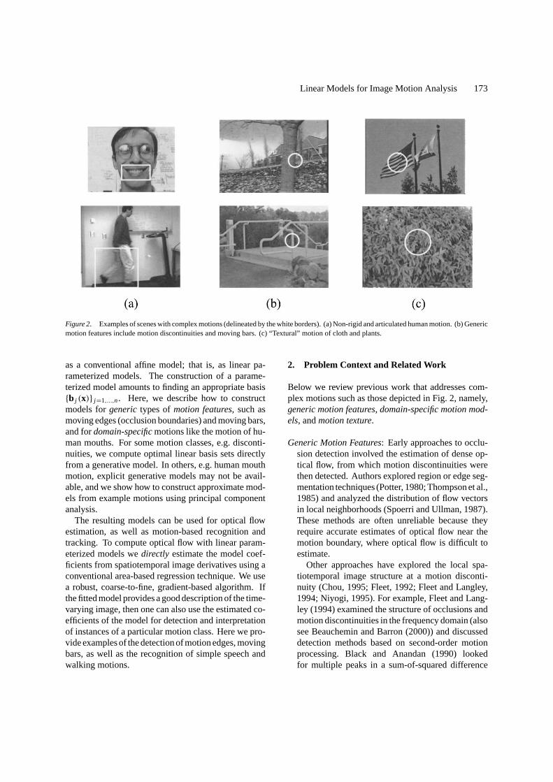
Figure 2. Examples of scenes with complex motions (delineated by the white borders). (a) Non-rigid and articulated human motion. (b) Genericmotion features include motion discontinuities and moving bars. (c) “Textural” motion of cloth and plants.

as a conventional affine model; that is, as linear pa-rameterized models. The construction of a parame-terized model amounts to finding an appropriate basis{b j (x)} j=1,...,n. Here, we describe how to constructmodels forgenerictypes ofmotion features, such asmoving edges (occlusion boundaries) and moving bars,and fordomain-specificmotions like the motion of hu-man mouths. For some motion classes, e.g. disconti-nuities, we compute optimal linear basis sets directlyfrom a generative model. In others, e.g. human mouthmotion, explicit generative models may not be avail-able, and we show how to construct approximate mod-els from example motions using principal componentanalysis.

The resulting models can be used for optical flowestimation, as well as motion-based recognition andtracking. To compute optical flow with linear param-eterized models wedirectly estimate the model coef-ficients from spatiotemporal image derivatives using aconventional area-based regression technique. We usea robust, coarse-to-fine, gradient-based algorithm. Ifthe fitted model provides a good description of the time-varying image, then one can also use the estimated co-efficients of the model for detection and interpretationof instances of a particular motion class. Here we pro-vide examples of the detection of motion edges, movingbars, as well as the recognition of simple speech andwalking motions.

2. Problem Context and Related Work

Below we review previous work that addresses com-plex motions such as those depicted in Fig. 2, namely,generic motion features, domain-specific motion mod-els, andmotion texture.

Generic Motion Features: Early approaches to occlu-sion detection involved the estimation of dense op-tical flow, from which motion discontinuities werethen detected. Authors explored region or edge seg-mentation techniques (Potter, 1980; Thompson et al.,1985) and analyzed the distribution of flow vectorsin local neighborhoods (Spoerri and Ullman, 1987).These methods are often unreliable because theyrequire accurate estimates of optical flow near themotion boundary, where optical flow is difficult toestimate.

Other approaches have explored the local spa-tiotemporal image structure at a motion disconti-nuity (Chou, 1995; Fleet, 1992; Fleet and Langley,1994; Niyogi, 1995). For example, Fleet and Lang-ley (1994) examined the structure of occlusions andmotion discontinuities in the frequency domain (alsosee Beauchemin and Barron (2000)) and discusseddetection methods based on second-order motionprocessing. Black and Anandan (1990) lookedfor multiple peaks in a sum-of-squared difference

174 Fleet et al.

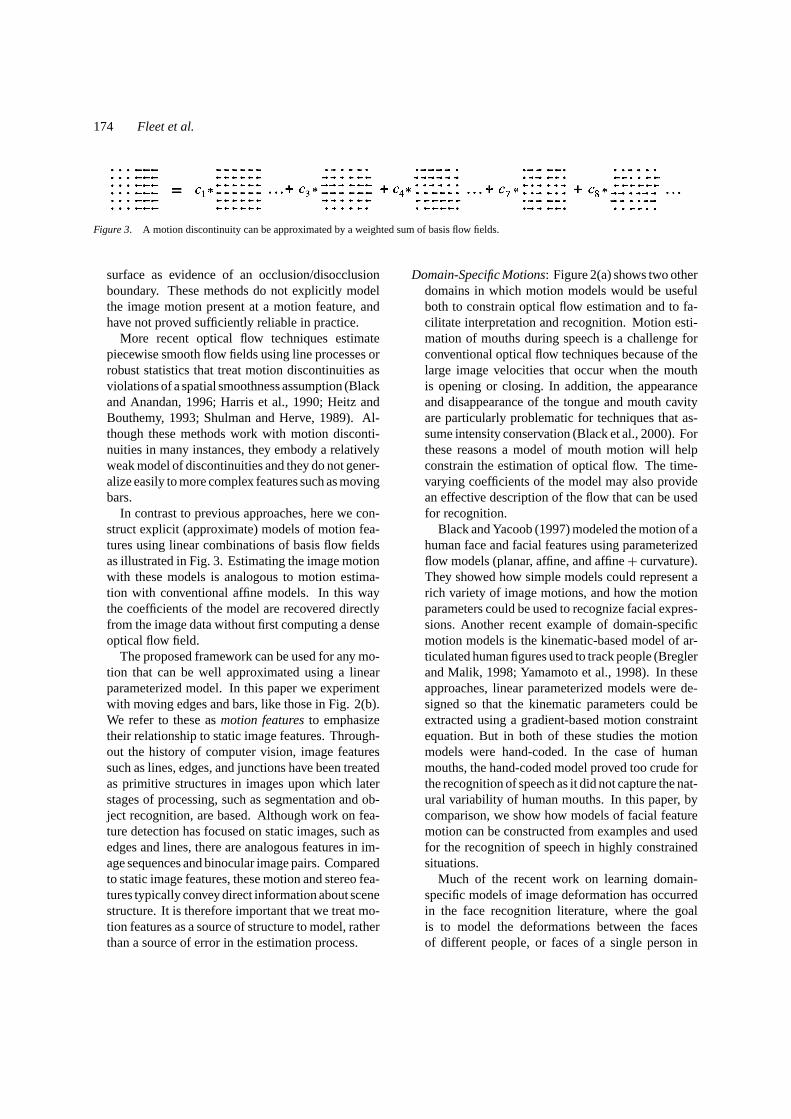
Figure 3. A motion discontinuity can be approximated by a weighted sum of basis flow fields.

surface as evidence of an occlusion/disocclusionboundary. These methods do not explicitly modelthe image motion present at a motion feature, andhave not proved sufficiently reliable in practice.

More recent optical flow techniques estimatepiecewise smooth flow fields using line processes orrobust statistics that treat motion discontinuities asviolations of a spatial smoothness assumption (Blackand Anandan, 1996; Harris et al., 1990; Heitz andBouthemy, 1993; Shulman and Herve, 1989). Al-though these methods work with motion disconti-nuities in many instances, they embody a relativelyweak model of discontinuities and they do not gener-alize easily to more complex features such as movingbars.

In contrast to previous approaches, here we con-struct explicit (approximate) models of motion fea-tures using linear combinations of basis flow fieldsas illustrated in Fig. 3. Estimating the image motionwith these models is analogous to motion estima-tion with conventional affine models. In this waythe coefficients of the model are recovered directlyfrom the image data without first computing a denseoptical flow field.

The proposed framework can be used for any mo-tion that can be well approximated using a linearparameterized model. In this paper we experimentwith moving edges and bars, like those in Fig. 2(b).We refer to these asmotion featuresto emphasizetheir relationship to static image features. Through-out the history of computer vision, image featuressuch as lines, edges, and junctions have been treatedas primitive structures in images upon which laterstages of processing, such as segmentation and ob-ject recognition, are based. Although work on fea-ture detection has focused on static images, such asedges and lines, there are analogous features in im-age sequences and binocular image pairs. Comparedto static image features, these motion and stereo fea-tures typically convey direct information about scenestructure. It is therefore important that we treat mo-tion features as a source of structure to model, ratherthan a source of error in the estimation process.

Domain-Specific Motions: Figure 2(a) shows two otherdomains in which motion models would be usefulboth to constrain optical flow estimation and to fa-cilitate interpretation and recognition. Motion esti-mation of mouths during speech is a challenge forconventional optical flow techniques because of thelarge image velocities that occur when the mouthis opening or closing. In addition, the appearanceand disappearance of the tongue and mouth cavityare particularly problematic for techniques that as-sume intensity conservation (Black et al., 2000). Forthese reasons a model of mouth motion will helpconstrain the estimation of optical flow. The time-varying coefficients of the model may also providean effective description of the flow that can be usedfor recognition.

Black and Yacoob (1997) modeled the motion of ahuman face and facial features using parameterizedflow models (planar, affine, and affine+ curvature).They showed how simple models could represent arich variety of image motions, and how the motionparameters could be used to recognize facial expres-sions. Another recent example of domain-specificmotion models is the kinematic-based model of ar-ticulated human figures used to track people (Breglerand Malik, 1998; Yamamoto et al., 1998). In theseapproaches, linear parameterized models were de-signed so that the kinematic parameters could beextracted using a gradient-based motion constraintequation. But in both of these studies the motionmodels were hand-coded. In the case of humanmouths, the hand-coded model proved too crude forthe recognition of speech as it did not capture the nat-ural variability of human mouths. In this paper, bycomparison, we show how models of facial featuremotion can be constructed from examples and usedfor the recognition of speech in highly constrainedsituations.

Much of the recent work on learning domain-specific models of image deformation has occurredin the face recognition literature, where the goalis to model the deformations between the facesof different people, or faces of a single person in


different poses (Beymer, 1996; Ezzat and Poggio,1996; Hallinan, 1995; Nastar et al., 1996; Vetter,1996; Vetter et al., 1997). Correspondences betweendifferent faces were obtained either by hand or by anoptical flow method, and were then used to learn alow-dimensional model. In some cases this involvedlearning the parameters of a physically-based de-formable object (Nastar et al., 1996). In others, a ba-sis set of deformation vectors was obtained (e.g., seework by Hallinan (1995) on learning “EigenWarps”).One of the main uses of the learned models has beenview-based synthesis, as in Vetter (1996), Vetter et al.(1997) and Cootes et al. (1998) for example.

Related work has focused on learning the defor-mation of curves or parameterized curve models(Baumberg and Hogg, 1994; Sclaroff and Pentland,1994). Sclaroff and Pentland (1994) estimatedmodes of deformation for silhouettes of non-rigidobjects. Sclaroff and Isidoro (1998) use a similar ap-proach to model the deformation of image regions.Like our method they estimate the linear coefficientsof the model directly from the image. Unlike our ap-proach, they did not learn the basis flows from opticalflow examples of the object being tracked, nor didthey use the coefficients for detection or recognition.

Motion Texture:The flags and bush shown in Fig. 2(c)illustrate another form of domain-specific motion,often called motion texture. Authors have exploredtexture models for synthesizing such textural mo-tions and frequency analysis techniques for rec-ognizing them (Nelson and Polana, 1992). Thesemotions typically exhibit complex forms of localocclusion and self shadowing that violate the as-sumption of brightness constancy. They also tend toexhibit statistical regularities at specific spatial andtemporal scales that make it difficult to find good lin-ear approximations. Experiments using linear mod-els to account for these motions (Black et al., 1997)suggest that such models may not be appropriate,and they therefore remain outside the scope of thecurrent work.

3. Constructing Parameterized Motion Models

The construction of a linear parameterized model for aparticular motion class involves finding a set ofbasisflow fieldsthat can be combined linearly to approximateflow fields in the motion class. In the case of motionfeatures, such as motion edges and bars, we begin withthe design of an idealized, generative model. From this

Figure 4. Example motion features and models for a motion dis-continuity and a moving bar. The parameters of the idealized modelsare the mean (DC) translational velocityut , the feature orientationθ , and the velocity change across the motion feature1u.

model we explicitly construct an approximate basis setusing steerable filters (Freeman and Adelson, 1991;Perona, 1995), yielding a basis ofsteerable flow fields.

With complex object motions, such as mouths orbushes, no analytical model exists. If an ensembleof training flow fields is available, then one can useprincipal component analysis (PCA) or independentcomponent analysis (ICA) (Bell and Sejnowski, 1997)to find a set of basis flow fields. A similar approachwas taken by Nayer et al. (1996) to model edges, bars,and corners in static images.

3.1. Models for Motion Features Using SteerableFlow Fields

First, consider the modeling of motion edges and barslike those in Fig. 4. The motion edge can be describedby a mean (DC) motion vectorut , an edge orientationθ , and a velocity change across the motion boundary1u. Letf(x; ut ,1u, θ)be the corresponding flow fieldover spatial positionsx = (x, y) in a circular imagewindow R. Becausef(x; ut ,1u, θ) is non-linear inthe feature parameters,ut ,1u, andθ , direct parameterestimation in the 5-dimensional space, without a goodinitial guess, can be difficult.

As depicted in Fig. 3, our approach is to approxi-matef(x; ut ,1u, θ) by its projection onto a subspacespanned by a collection ofn basis flow fieldsb j (x) ,

f(x; ut ,1u, θ) ≈ u(x; c) =n∑

j=1

cj b j (x). (2)

Although the basis flow fields could be learned fromexamples using Principal Component Analysis, herewe constructsteerablesets of basis flow fields. Theseare similar to those learned using PCA up to rotationsof invariant subspaces. The basis flow fields are steer-able in orientation and velocity, and provide reason-ably accurate approximations to the motion features of

176 Fleet et al.

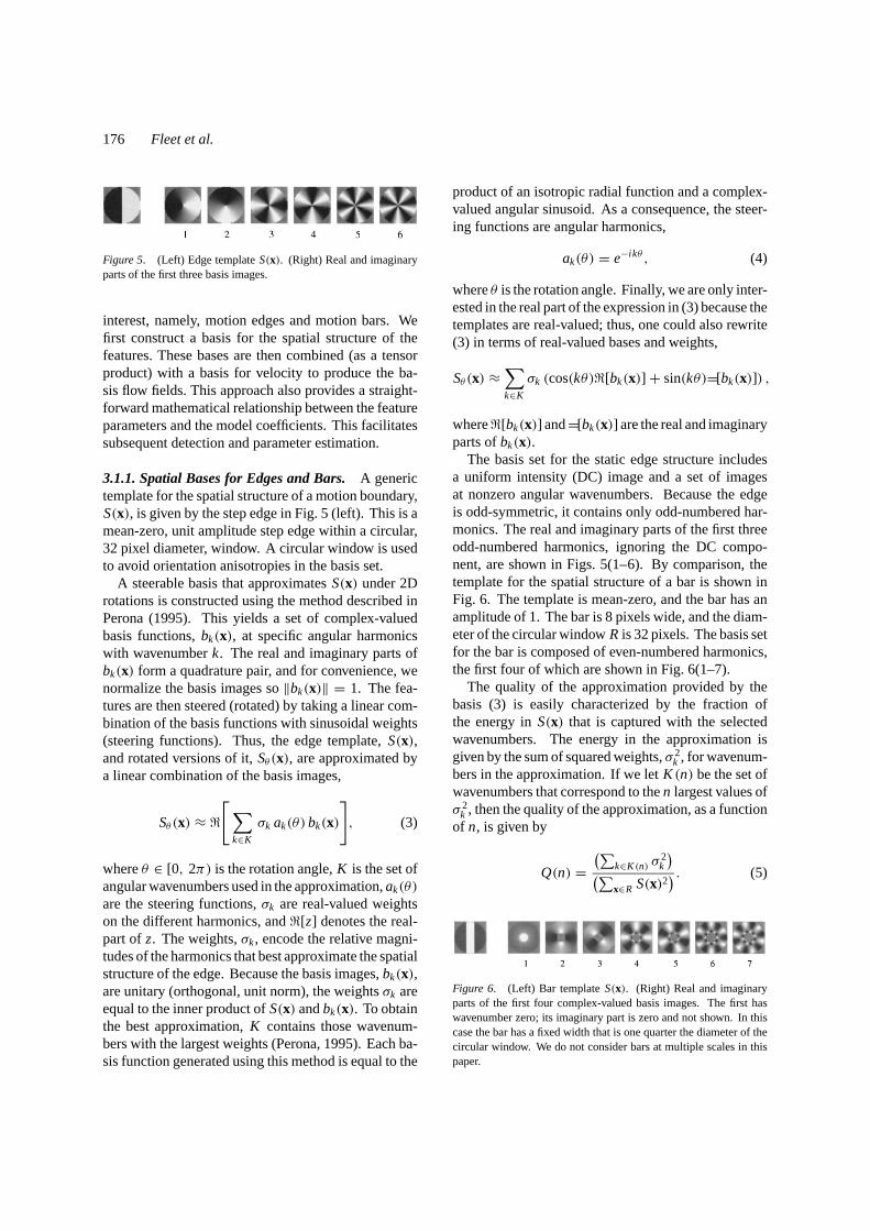
Figure 5. (Left) Edge templateS(x). (Right) Real and imaginaryparts of the first three basis images.

interest, namely, motion edges and motion bars. Wefirst construct a basis for the spatial structure of thefeatures. These bases are then combined (as a tensorproduct) with a basis for velocity to produce the ba-sis flow fields. This approach also provides a straight-forward mathematical relationship between the featureparameters and the model coefficients. This facilitatessubsequent detection and parameter estimation.

3.1.1. Spatial Bases for Edges and Bars.A generictemplate for the spatial structure of a motion boundary,S(x), is given by the step edge in Fig. 5 (left). This is amean-zero, unit amplitude step edge within a circular,32 pixel diameter, window. A circular window is usedto avoid orientation anisotropies in the basis set.

A steerable basis that approximatesS(x) under 2Drotations is constructed using the method described inPerona (1995). This yields a set of complex-valuedbasis functions,bk(x), at specific angular harmonicswith wavenumberk. The real and imaginary parts ofbk(x) form a quadrature pair, and for convenience, wenormalize the basis images so‖bk(x)‖ = 1. The fea-tures are then steered (rotated) by taking a linear com-bination of the basis functions with sinusoidal weights(steering functions). Thus, the edge template,S(x),and rotated versions of it,Sθ (x), are approximated bya linear combination of the basis images,

Sθ (x) ≈ <[∑

k∈K

σk ak(θ) bk(x)

], (3)

whereθ ∈ [0, 2π) is the rotation angle,K is the set ofangular wavenumbers used in the approximation,ak(θ)

are the steering functions,σk are real-valued weightson the different harmonics, and<[z] denotes the real-part ofz. The weights,σk, encode the relative magni-tudes of the harmonics that best approximate the spatialstructure of the edge. Because the basis images,bk(x),are unitary (orthogonal, unit norm), the weightsσk areequal to the inner product ofS(x) andbk(x). To obtainthe best approximation,K contains those wavenum-bers with the largest weights (Perona, 1995). Each ba-sis function generated using this method is equal to the

product of an isotropic radial function and a complex-valued angular sinusoid. As a consequence, the steer-ing functions are angular harmonics,

ak(θ) = e−ikθ , (4)

whereθ is the rotation angle. Finally, we are only inter-ested in the real part of the expression in (3) because thetemplates are real-valued; thus, one could also rewrite(3) in terms of real-valued bases and weights,

Sθ (x) ≈∑k∈K

σk (cos(kθ)<[bk(x)] + sin(kθ)=[bk(x)]) ,

where<[bk(x)] and=[bk(x)] are the real and imaginaryparts ofbk(x).

The basis set for the static edge structure includesa uniform intensity (DC) image and a set of imagesat nonzero angular wavenumbers. Because the edgeis odd-symmetric, it contains only odd-numbered har-monics. The real and imaginary parts of the first threeodd-numbered harmonics, ignoring the DC compo-nent, are shown in Figs. 5(1–6). By comparison, thetemplate for the spatial structure of a bar is shown inFig. 6. The template is mean-zero, and the bar has anamplitude of 1. The bar is 8 pixels wide, and the diam-eter of the circular windowR is 32 pixels. The basis setfor the bar is composed of even-numbered harmonics,the first four of which are shown in Fig. 6(1–7).

The quality of the approximation provided by thebasis (3) is easily characterized by the fraction ofthe energy inS(x) that is captured with the selectedwavenumbers. The energy in the approximation isgiven by the sum of squared weights,σ 2

k , for wavenum-bers in the approximation. If we letK (n) be the set ofwavenumbers that correspond to then largest values ofσ 2

k , then the quality of the approximation, as a functionof n, is given by

Q(n) =(∑

k∈K (n) σ2k

)(∑x∈R S(x)2

) . (5)

Figure 6. (Left) Bar templateS(x). (Right) Real and imaginaryparts of the first four complex-valued basis images. The first haswavenumber zero; its imaginary part is zero and not shown. In thiscase the bar has a fixed width that is one quarter the diameter of thecircular window. We do not consider bars at multiple scales in thispaper.


Figure 7. Fraction of energy in the edge model (a) and the barmodel (b) that is captured in the linear approximation as a functionof the number of complex-valued basis functions used.

This quantity is shown in Fig. 7 for the edge and thebar. In the case of the edge, the three harmonics shownin Fig. 5 account for approximately 94% of the energyin the edge template. With the bar, the four harmonicsshown in Fig. 6 account for over 90% of the energy.

3.1.2. Basis Flow Fields for Motion Edges and Bars.The basis flow fields for the motion features are formedby combining a basis for velocity with the basis for thespatial structure of the features. Two vectors,(1, 0)T

and(0, 1)T , provide a basis for translational flow. Thebasis flow fields for the horizontal and vertical compo-nents of the motion features are therefore given by

bhk(x) =

(bk(x)

0

), bvk(x) =

(0

bk(x)

). (6)

For each angular wavenumber,k, there are four real-valued flow fields. These are the real and imaginaryparts ofbk(x), each multiplied by the horizontal andthe vertical components of the velocity basis.

Figure 8. Steerable basis flow fields for occluding edges. (Top) Flow fields are depicted as images in which the horizontal (u) component ofthe flow is the top half, and the vertical (v) component is the bottom half. Black indicates motion to the left or up respectively. Gray is zeromotion and white is motion to the right or down. (Bottom) Basis flow fields (3–10) depicted as subsampled vector fields.

The real and imaginary parts of the basis flow fieldsfor the motion edge are depicted in Fig. 8(1–10). Twoangular harmonics are shown, each with 4 real-valuedflow fields, along with the DC basis functions that en-code constant translational velocity. One can see thatsome of the basis flow fields bear some similarity tononlinear shear and expansion/compression.

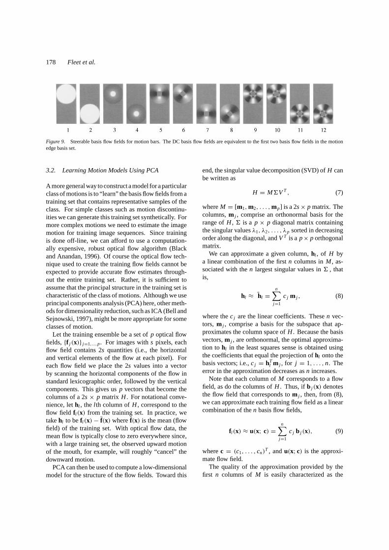
Figure 9(3–12) show the basis flow fields for themotion bar. Here, Fig. 9(3–4) encode the basis flowfields for wavenumberk = 0, for which only the real-part is nonzero. Figure 9(5–8) and (9–12) show thereal-valued basis flow fields for wavenumbersk = 2andk = 4 respectively.

Note that the basis flow fields for motion edges andbars, based on odd and even wavenumbers respectively,are orthogonal. Thus, when one wants to detect bothfeatures, the basis sets can be combined trivially toform a single basis set. We demonstrate them individ-ually, and together in the experiements shown below inSection 5.

Finally, it is also useful to note that these basis flowfields are approximate. With only a small number ofwavenumbers the basis flow fields span a relativelycrude approximation to a step motion discontinuity.Second, since they approximate only the instantaneousnature of the image velocity field, the bases flow fieldsdo not explicitly model the pixels that are occluded ordisoccluded by the moving feature. This results in un-modeled brightness variations at the feature boundariesthat must be coped with when estimating the coeffi-cients. Our estimation approach described in Section 4uses robust statistical techniques for this purpose.

178 Fleet et al.

Figure 9. Steerable basis flow fields for motion bars. The DC basis flow fields are equivalent to the first two basis flow fields in the motionedge basis set.

3.2. Learning Motion Models Using PCA

A more general way to construct a model for a particularclass of motions is to “learn” the basis flow fields from atraining set that contains representative samples of theclass. For simple classes such as motion discontinu-ities we can generate this training set synthetically. Formore complex motions we need to estimate the imagemotion for training image sequences. Since trainingis done off-line, we can afford to use a computation-ally expensive, robust optical flow algorithm (Blackand Anandan, 1996). Of course the optical flow tech-nique used to create the training flow fields cannot beexpected to provide accurate flow estimates through-out the entire training set. Rather, it is sufficient toassume that the principal structure in the training set ischaracteristic of the class of motions. Although we useprincipal components analysis (PCA) here, other meth-ods for dimensionality reduction, such as ICA (Bell andSejnowski, 1997), might be more appropriate for someclasses of motion.

Let the training ensemble be a set ofp optical flowfields, {f j (x)} j=1,...,p. For images withs pixels, eachflow field contains 2s quantities (i.e., the horizontaland vertical elements of the flow at each pixel). Foreach flow field we place the 2s values into a vectorby scanning the horizontal components of the flow instandard lexicographic order, followed by the verticalcomponents. This gives usp vectors that become thecolumns of a 2s× p matrix H . For notational conve-nience, lethl , the l th column ofH , correspond to theflow field fl (x) from the training set. In practice, wetakehl to befl (x)− f(x) wheref(x) is the mean (flowfield) of the training set. With optical flow data, themean flow is typically close to zero everywhere since,with a large training set, the observed upward motionof the mouth, for example, will roughly “cancel” thedownward motion.

PCA can then be used to compute a low-dimensionalmodel for the structure of the flow fields. Toward this

end, the singular value decomposition (SVD) ofH canbe written as

H = M6VT , (7)

whereM = [m1,m2, . . . ,mp] is a 2s× p matrix. Thecolumns,m j , comprise an orthonormal basis for therange ofH , 6 is a p× p diagonal matrix containingthe singular valuesλ1, λ2, . . . , λp sorted in decreasingorder along the diagonal, andVT is a p× p orthogonalmatrix.

We can approximate a given column,hl , of H bya linear combination of the firstn columns inM , as-sociated with then largest singular values in6 , thatis,

hl ≈ hl =n∑

j=1

cj m j , (8)

where thecj are the linear coefficients. Thesen vec-tors, m j , comprise a basis for the subspace that ap-proximates the column space ofH . Because the basisvectors,m j , are orthonormal, the optimal approxima-tion to hl in the least squares sense is obtained usingthe coefficients that equal the projection ofhl onto thebasis vectors; i.e.,cj = hT

l m j , for j = 1, . . . ,n. Theerror in the approximation decreases asn increases.

Note that each column ofM corresponds to a flowfield, as do the columns ofH . Thus, ifb j (x) denotesthe flow field that corresponds tom j , then, from (8),we can approximate each training flow field as a linearcombination of then basis flow fields,

fl (x) ≈ u(x; c) =n∑

j=1

cj b j (x), (9)

wherec = (c1, . . . , cn)T , andu(x; c) is the approxi-

mate flow field.The quality of the approximation provided by the

first n columns of M is easily characterized as the


Figure 10. Modeling mouth motion. (a) A subject’s head is tracked using a planar model of image motion and the motion of the mouth isestimated relative to this head motion. (b) Example frames from the 3000 image training set of a person saying several words, and changingfacial expressions throughout several seconds of video.

fraction of the variance of the training set that is ac-counted for by then components:

Q(n) =(∑n

j=1 λ2j

)(∑p

j=1 λ2j

) . (10)

A good approximation (i.e., whenQ(n) approaches 1)is obtained when the singular valuesλ j are relativelysmall for j > n. If the singular values rapidly decreaseto zero asj increases thenQ(n) rapidly increases to-wards 1, and a low-dimensional linear model providesan accurate approximation to the flow fields in the train-ing set.

3.2.1. Example: Mouth Motion. As an example, welearn a parameterized model of mouth motion for asingle speaker. We collected a 3000 image training se-quence in which the speaker moved their head, spokenaturally, and made repeated utterances of four testwords, namely, “center,” “print,” “track,” and “release.”

Figure 11. (Left) First 8 basis flow fields for non-rigid mouth motion. (Right) Fraction of variance from the mouth training ensemble that iscaptured in the model, as a function of the number of basis flow fields. The first six basis flow fields account for approximately 90% of thevariance.

As illustrated in Fig. 10, the subject’s head was trackedand stabilized using a planar motion model to removethe face motion (see Black and Yacoob (1997) for de-tails). This stabilization allows isolation of the mouthregion, examples of which are shown in Fig. 10. Themotion of the mouth region was estimated relative tothe head motion using the dense optical flow methoddescribed in Black and Anandan (1996). This results ina training set of mouth flow fields between consecutiveframes.

The mean flow field of this training set is computedand subtracted from each of the training flow fields.The mean motion is nearly zero and accounts for verylittle of the variation in the training set (1.7%). Themodified training flow fields are then used in the SVDcomputation described above. Since the image motionof the mouth is highly constrained, the optical flowstructure in the 3000 training flow fields can be approx-imated using a small number of principal componentflow fields. In this case, 91.4% of the variance in thetraining set is accounted for by the first seven compo-nents (shown in Fig. 11). The first component alone

180 Fleet et al.

accounts for approximately 71% of the variance. It isinteresting to compare this learned basis set with thehand-constructed basis used to model mouth motion inBlack and Yacoob (1997). The hand-constructed basiscontained seven flow fields representing affine motionplus a vertical curvature basis to capture mouth cur-vature. In contrast to the learned basis set, the hand-constructed set accounts for only 77.5% of the variancein the training set.

3.3. Designing Basis Sets

It is also possible to “design” basis sets with particularproperties. In many cases one may wish to have abasis that spans affine motion plus some higher-orderdeformation. This may be true for mouth motion aswell as for rigid scenes. For example, we applied thelearning method to a training set composed of patchesof optical flow (roughly 40× 40 sized regions) takenrandomly from the Yosemite sequence which containsa rigid scene and a moving camera (Barron et al., 1994).The first six basis flows accounted for 99.75% of thevariance, and they appear to span affine motions. Tocompare this with an exact affine model, we projectedall affine motion out of the training flow fields, and thenperformed PCA on the residual flows fields. The affinemodel accounts for 99.68% of the variance suggestingthat, for this sequence and others like it, a local affinemodel is sufficient.

To construct a basis to explicitly represent affine mo-tion plus some non-rigid deformation from a trainingset, we first construct an orthonormal set of affine basisflows,

u(x; c) =[

u(x; c)v(x; c)

]=[

c1+ c2x + c3y

c4+ c5x + c6y

],

the affine basis flowsb j (x) of which are illustrated inFig. 1. We project affine structure out of the train-ing set using a Gram-Schmidt procedure (Golub andvan Loan, 1983), and then apply PCA to the remain-ing flow fields. More precisely, in vector form, let{m j } j=1,...,6 denote an orthonormal basis for affine mo-tion, and let the original ensemble of training flow fieldsbe expressed as{h j } j=1,...,p. The magnitude of theprojection of hl onto the affine basis vectorsm j isgiven bycl j = hT

l m j . Then, affine structure can besubtracted out ofhl to produce the new training flow

field, h∗l , given by

h∗l = hl −6∑

j=1

cl j m j . (11)

Finally, we perform PCA on the new training set, eachflow field of which is now orthogonal to the affine ba-sis set. We choose the firstn basis flows from thisdeformation basis and then construct our basis set with6+ n flow fields in which the first six represent affinemotion. We now have a basis that is guaranteed torepresent affine motion plus some learned deformationfrom affine. This process can be also be applied toorthogonal basis sets other than affine.

4. Direct Estimation of Model Coefficients

Given a basis set of flow fields for a particular motionclass, we wish to estimate the model coefficients froman image sequence. We then wish to use these coef-ficients to detect instances of the motion classes. Todetect features in static images using linear parame-terized feature models (e.g., (Nayar et al., 1996)), themodel coefficients are obtained by convolving the im-age with the basis images. With motion models wecannot take the same approach because the motionfield is unknown. One could first estimate the denseflow field using generic smoothness constraints andthen filter the result. However, the strong constraintsprovided by parameterized models have been shownto produce more accurate and stable estimates of im-age motion than generic dense flow models (Ju et al.,1996). Therefore we apply our new motion modelsin the same way that affine models have been usedsuccessfully in the past; we make the assumption ofbrightness constancy and estimate the linear coeffi-cients directly from the spatial and temporal imagederivatives.

More formally, within an image region,R, we wishto find the linear coefficientsc of a parameterized mo-tion model that satisfy the brightness constancy as-sumption,

I (x, t + 1)− I (x− u(x; c), t) = 0 ∀x ∈ R, (12)

whereu(x; c) is given by (1). Eq. (12) states that theimage, I , at framet + 1 is a warped version of theimage at timet .


In order to estimate the model coefficients we mini-mize the following objective function

E(c) =∑x∈R

ρ(I (x, t + 1)− I (x− u(x; c), t), σ ).

(13)

Here,σ is a scale parameter andρ(·, σ ) is a robust errorfunction applied to the residual error

1I (x; c) = I (x, t + 1)− I (x− u(x; c), t) . (14)

Large residual errors may be caused by changes in im-age structure that are not accounted for by the learnedflow model. Because of the discontinuous nature of themotion models used here and the expected violationsof brightness constancy, it is important that the estima-tor be robust with respect to these “outliers”. For theexperiments below we takeρ(·, σ ) to be

ρ(r, σ ) = r 2

σ 2+ r 2,

which was proposed in Geman and McClure (1987)and used successfully for flow estimation in Black andAnandan (1996). The parameter,σ , controls the shapeof ρ(·, σ ) to minimize the influence of large residualerrors on the solution.

Equation (13) can be minimized in a number of waysincluding coordinate descent (Black and Anandan,1996), random sampling (Bab-Hadiashar and Suter,1998), or iteratively reweighted least squares (Ayer andSawhney, 1995; Hager and Belhumeur, 1996). Herewe use a coarse-to-fine, iterative, coordinate descentmethod. To formulate an iterative method to minimize(13), it is convenient to first rewrite the model coeffi-cient vector in terms of an initial guessc and an updateδc. This allows us to rewrite (13) as

E(δc; c) =∑x∈R

ρ(I (x, t + 1)

− I (x− u(x; c+ δc), t), σ ). (15)

Given an estimate,c, of the motion coefficients (ini-tially zero), the goal is to estimate the update,δc, thatminimizes (15);c then becomesc+ δc. To minimize(15) we first approximate it by linearizing the residual,1I (x; c+ δc), with respect to the update vectorδc togive

E(δc; c) =∑x∈R

ρ(u(x; δc)T E∇ I (x− u(x; c), t)

+1I (x; c), σ ), (16)

where E∇ I (x − u(x; c), t) denotes the spatial imagegradient at timet , warped by the current motionestimateu(x; c) using bilinear interpolation. Note thatthe brightness constancy assumption has been approx-imated by an optical flow constraint equation that islinear inδc. Finally, note that in minimizing (16), thesearch algorithm described below typically generatessmall update vectors,δc. Because the objective func-tion in (16) satisfiesE(δc; c) = E(δc; c)+ O(‖δc‖2),the approximation error vanishes as the update,δc, isreduced to zero.

It is also worth noting that the gradient term in(16) does not depend onδc. This avoids the needto rewarp the image and recompute the image gradi-ent at each step of the coordinate descent. In fact,the image gradient in (16) can be pre-multiplied bythe basis flows fields since these quantities will notchange during the minimization ofE(δc; c). Hagerand Belhumeur (1996) used this fact for real-time affinetracking.

To minimize (15) we use a coarse-to-fine controlstrategy with a continuation method that is an extensionof that used by Black and Anandan (1996) for estimat-ing optical flow with affine and planar motion models.We construct a Gaussian pyramid for the images at timet andt+1. The motion coefficients,cl , determined at acoarse scale,l , are used in the minimization at the nextfiner scale,l +1. In particular, the motion coefficients,cl + δcl , from the coarse level are first multiplied by afactor of two (to reflect the doubling of the image sizeat levell + 1) to produce the initial guesscl+1 at levell + 1. These coefficients are then used in (16) to warpthe image at timet + 1 towards the image at timet atlevel l + 1, from whichE(δcl+1; cl+1) is minimized tocompute the next updateδcl+1.

The basis flow fields at a coarse scale are smoothed,subsampled versions of the basis flows at the next finerscale. These coarse-scale basis vectors may deviateslightly from orthogonality but this is not significantgiven our optimization scheme. We also find that it isimportant for the stability of the optimization to usefewer basis flow fields at the coarsest levels, increas-ing the number of basis flow fields as the estimationproceeds from coarse to fine. The basis flow fieldsto be used at the coarsest levels are those that corre-spond to the majority of the energy in the training set(for domain-specific models) or in the approximationto the model feature (for motion features). The flowsfields used at the coarse levels are typically smoother(i.e., lower wavenumbers), and therefore they do not

182 Fleet et al.

alias or lose significant signal power when they aresubsampled.

At each scale, given a starting estimateu(x; cl ), weminimize E(δc; cl ) in (16) using a coordinate descentprocedure. The partial derivatives ofE(δc; cl )with re-spect toδc are straightforward to derive. When the up-date vector is complex-valued, as it is with our motionfeature models, we differentiateE(δc; cl ) with respectto both the real and imaginary parts ofδc. To deal withthe non-convexity of the objective function, the robustscale parameter,σ , is initially set to a large value andthen slowly reduced. For the experiments below,σ

is lowered from 25√

2 to 15√

2 by a factor of 0.95 ateach iteration. Upon completion of a fixed number ofdescent steps (or when a convergence criterion is met),the new estimate for the flow coefficients is taken to becl + δc.

4.1. Translating Disk Example

To illustrate the estimation of the model coefficientsand the detection of motion discontinuities, we con-structed a synthetic sequence of a disk translatingacross a stationary background (Fig. 12(a)). Both thedisk and the background had similar fractal textures, sothe boundary of the stationary disk is hard to see in asingle image. The image size was 128× 128, the diskwas 60 pixels wide, and the basis flow fields were 32pixels wide.

Optical flow estimation with a motion feature basisproduces a set of coefficients for each neighborhood inthe image. Here, the model coefficients were estimatedfrom neighborhoods centered at each pixel (so long asneighborhoods did not overlap the image boundary).

Figure 12. Translating Disk. (a) Image of the disk and background(same random texture). (b) Estimated flow field superimposed onthe disk. (1–10) Recovered coefficient images for the motion edgebasis set. For display the responses of coefficients corresponding toeach wavenumber are scaled independently to maximize the rangeof gray levels shown.

This yields coefficient values at each pixel that can beviewed as images (i.e., two real-valued images for eachcomplex-valued coefficient). Figure 12(1–10) showsthe real-valued coefficients that correspond to the basisflow fields for the motion edge model in Fig. 8(1–10).Figure 12(1 and 2) depicts coefficients for horizontaland vertical translation; one can infer the horizontalvelocity of the disk. Figure 12(3–10) corresponds tobasis flow fields with horizontal and vertical motion atwavenumbers 1 and 3. In these images one can see thedependence of coefficient values on the wavenumber,the orientation of the motion edge, and the directionof the velocity difference. As described below, it isthe structure in these coefficients that facilitates thedetection of the motion edges.

4.2. Human Mouth Motion Example

Estimation of human mouth motion is challenging dueto non-rigidity, self occlusion, and high velocities rel-ative to standard video frame rates. Consider the twoconsecutive frames from a video sequence shown inFig. 13. Note the large deformations of the lips, and thechanges in appearance caused by the mouth opening.This makes optical flow estimation with standard denseflow methods difficult. For example, Fig. 13(c) shows aflow field estimated with a robust dense method (Blackand Anandan, 1996). Some of the flow vectors differwidely from their neighbors. By comparison, the flowfield estimated with the learned model is constrained tobe a type of mouth motion, which yields the smootherflow field in Fig. 13(d). Of course, we cannot say whichof these two flow fields is “better” in this context; eachminimizes a measure of brightness constancy. In thefollowing section we will be concerned with recogni-tion, and in that scenario we wish to constrain the esti-mation to valid mouth motions such as that representedby Fig. 13(d).

Figure 13. Estimating mouth motion. (a, b) Mouth regions of twoconsecutive images of a person speaking. (c) Flow field estimatedusing dense optical flow method. (d) Flow field estimated using thelearned model with 6 basis flow fields.


5. Detection of Parameterized Motion Models

From the estimated linear model coefficients, we areinterested in detecting and recognizing types of motion.We first consider the detection of motion edges andbars. Following that, we examine the recognition oftime-varying motions in the domains of mouths andpeople walking.

5.1. Motion Feature Detection

Given the estimated linear coefficients,c, we wish todetect occurrences of motion edges and motion bars,and to estimate their parameters, namely, the two com-ponents of the mean velocityut = (ut , vt ), the two com-ponents of the velocity change1u = (1u,1v)T , andthe feature orientationθ . The linear parameterizedmodels for motion edges and bars were designed sothat any motion edge or bar can be well approximatedby some linear combination of the basis flow fields. Butnot all linear combinations of the basis flow fields cor-respond to valid motion features. Rather, the motionsfeatures lie on a lower-dimensional, nonlinear manifoldwithin the subspace spanned by the basis flow fields. InNayar (1996), the detection problem for static featureswas addressed by taking tens of thousands of examplefeatures and projecting them onto the basis set. Thesetraining coefficients provided a dense sampling of amanifold in the subspace spanned by the basis vectors.Given the coefficients corresponding to an image fea-ture, the closest point on the manifold was found. If anestimated coefficient vectorc lies sufficiently close tothe manifold then the parameters of the nearest trainingexample were taken to be the model parameters. Alter-natively, one could interpolate model parameters overthe manifold (Bregler and Omohundro, 1995). This ap-proach to detection is appropriate for complex featureswhere no underlying model is available (e.g., the mo-tion of human mouths (Black et al., 1997)). By compar-ison, the underlying models of motion features are rel-atively simple. In these cases we therefore solve for thefeature parameters directly from the linear coefficients.

5.1.1. Nonlinear Least-Squares Estimation.Givenan estimated flow field,u(x; c), obtained with the ro-bust iterative method outlined in Section 4, we wish todetect the presence of a motion feature and to estimateits parameters(ut ,1u, θ). That is, we wish to esti-mate the parameters that produce the idealized flowfield, f(x; ut ,1u, θ), that is closest to the estimated

flow field,u(x; c). We also want to decide whether themodel is a sufficiently good fit to allow us to infer thepresense of the feature. Because there are five inde-pendent feature parameters, the orthogonal projectionof f(x; ut ,1u, θ) onto the basis flow fields lies on a5-dimensional nonlinear manifold. It suffices to findthe flow field on this manifold that is closest tou(x; c).

Let um(x; ut ,1u, θ) denote the projection of theidealized flow fieldf(x; ut ,1u, θ), onto the linearsubspace. Using the form of the basis flow fields in(3), (4) and (6), one can show thatum(x; ut ,1u, θ)has the form

um(x; ut ,1u, θ)

= ut +<[∑

k∈K

σk e−ikθ(1u bh

k(x)+1v bvk(x)) ].

(17)

Then, for a regionR, we seek the five parameters(ut ,1u, θ) that minimize∑

x∈R

‖um(x; ut , 1u, θ) − u(x; c)‖2. (18)

To formulate the solution it is convenient to explicitlyexpress the estimated flow field,u(x; c), using the samenotation for the basis flow fields:

u(x; c) = udc + <[∑

k∈K

(αkbh

k(x) + βkbvk(x))],

(19)

whereudc is a 2-vector that corresponds to the coeffi-cients associated with the DC basis flow fields, andαk

andβk are the estimated (complex-valued) coefficientsthat correspond to the horizontal and vertical compo-nents of the basis flow fields with wavenumberk.

The basis in which bothum(x; ut ,1u, θ)andu(x; c)are expressed (i.e.,{bh

k(x), bvk(x)}k∈K ) is orthogonal.

Therefore, to minimize (18) it suffices to find the fea-ture parameters that minimize the sum of squared dif-ferences between model coefficients and the estimatedcoefficients. Thus, the translational velocity is givendirectly byut = udc. The remaining parameters,1uandθ , are found by minimizing

Em(1u, θ) =∑k∈K

‖(αk, βk)− σk e−ikθ (1u,1v)‖2,

(20)

given a sufficiently good initial guess.

184 Fleet et al.

The least-squares minimization enforces two con-straints on the feature parameters. First, the velocitydifference,1u, must be consistent over all angular har-monics. Second, the orientation of the motion feature,θ , must be consistent across all of the angular harmon-ics and both components of flow. The constraint on1u is related to the magnitudes of the complex-valuedmodel coefficients, while the constraint onθ concernstheir phase values. To obtain an initial guess for mini-mizing Em(1u, θ), we first decouple these constraints.This provides a suboptimal, yet direct, method for es-timatingθ and1u.

5.1.2. Direct Estimation of Velocity Change.To for-mulate a constraint on1u = (1u,1v)T it is conve-nient to collect the complex-valued coefficients of themodel flow field in (17) into an outer product matrix

M=1u (σk1 e−ik1θ , . . . , σkn e−iknθ ) (21)

=(1u σk1 e−ik1θ . . . 1u σkn e−iknθ

1v σk1 e−ik1θ . . . 1v σkn e−iknθ

), (22)

wheren is the number of angular harmonics inK , andfor 1 ≤ j ≤ n, let kj denote the wavenumbers inK with weightsσki . The top row ofM contains themodel coefficients for the horizontal components of themodel velocity field. The second row ofM containsthe model coefficients for the vertical components ofum(x; ut ,1u, θ).

To obtain a set of transformed model coefficients thatdepend solely on1u, we then constructA = M M∗T ,whereM∗T is the conjugate transpose ofM . Becauseof the separability of the model coefficients with re-spect to1u and θ , as shown in (21),A reduces to(σ 2

k1+ · · · + σ 2

kn)1u1ut , the components of which

are independent ofθ . For example, in the case of themotion edge, with the estimated coefficientsα1, α3, β1

andβ3, let

M =(α1 α3

β1 β3

), A = M M∗T . (23)

If the estimated flow field,u(x; c), were on the featuremanifold, then the singular vector associated with thelargest singular value,e1, of A should give the direc-tion of the velocity. Thus, the estimate of the velocitychange,1u0, is obtained by scaling this singular vector

by√

e1/(σ21 + σ 2

3 ).Moreover, if the estimated coefficients lie on the fea-

ture manifold, then the rank ofA in (23) should be 1.

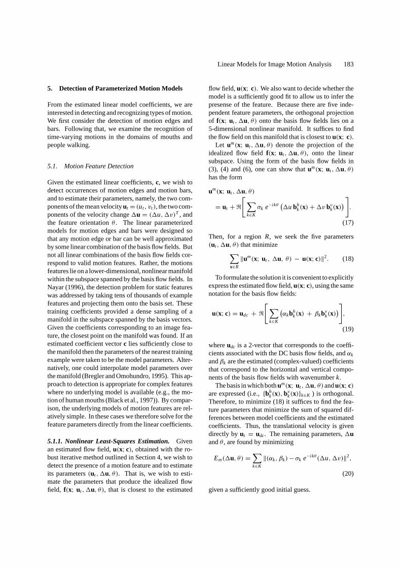
Figure 14. Translating Disk. (a) Raw orientation estimates fromdirect method. Black pixels indicate that no estimate was possible.Intensity varies from white to dark grey as orientation goes fromπ/2 to−π/2. (b, c) Confidence measures from velocity constraintand orientation constraint. (d) Orientation estimates masked by jointconfidence measure.

This suggests that we can use the ratio of the singularvalues,e1 ≥ e2, to determine the quality of the modelfit. A measure of the consistency of the estimated co-efficients with the model is given byr = (e2 + a)/e1.Here,r is close to zero where the coefficients satisfythe constraint and large otherwise;a is a small con-stant that helps to avoid instability when both singularvalues are extremely small. We useCv = exp[−r 2]as a confidence measure derived from this constraint,an image of which is shown for the disk sequence inFig. 14(b).

5.1.3. Direct Estimation of Spatial Orientation.Once the velocity parameters have been estimated, wecan use the initial estimate,1u0, along with the matrixM in (23) to obtain a set of transformed measurementsthat, according to the model, depend only on the spatialstructure of the motion feature. In particular, given thetrue velocity change1u, it is easy to show from (21)that the product1uTM has the form

1uTM = ‖1u‖2 (σk1 e−i k1 θ , . . . , σkn e−i kn θ).

(24)

From this it is clear that the orientationθ is availablein the phase of the elements of1uTM .

To obtain an initial orientation estimateθ0, we formthe productz = 1uT

0 M , using the estimated velocitychange1u0 and the matrix of estimated coefficientsM .To obtainθ0 fromzwe divide the phase of each compo-nent ofz according to its corresponding wavenumber(taking phase wrapping into account), and take theiraverage. According to the model, ignoring noise, theresulting phase values should then be equal, and com-puting their average yields the orientation estimationθ0. Figure 14(a) shows theθ0 as a function of imageposition for the Disk Sequence.


The variance of the normalized phases also gives usa measure of how well the estimated coefficients satisfythe model. For the edge model, where only two harmon-ics are used, we expect that1φ = φ1−φ3/3= 0 whereφk is the phase of the component ofz at wavenumberk. As a simple confidence measure for the quality ofthe model fit, Fig. 14(c) showsCθ = exp(−1φ2) forthe disk sequence.

5.1.4. Least-Squares Estimation and Detection.Thedirect method provides initial estimates of orientationθ0 and velocity change1u0, with confidence measures,Cv andCθ . We find that these estimates are usuallyclose to the least-squares estimates we seek in (20). Theconfidence measures can be used to reject coefficientvectors that are far from the feature manifold. Forexample, Fig. 14(d) shows orientation estimates whereCv Cθ > 0.1.

Given these initial estimates,θ0 and1u0, we usea gradient descent procedure to findθ and1u thatminimizeEm(1u, θ) in (20). Feature detection is thenbased on the squared error at the minima divided bythe energy in the subspace coefficients, i.e.,P =∑

k(|αk|2 + |βk|2). We find that the reliability of thedetection usually improves asP increases. To ex-ploit this, we use a simple confidence measure of theform

C = c(P) e−E/P. (25)

wherec(P)= e−κ/P andκ is a positive scalar that de-pends on noise levels. In this way, asP decreases therelative errorE/P must decrease for our confidencemeasure,C, to remain constant.

Figure 15(a) shows the confidence measureC giventhe least-squares estimates of the motion edge param-eters, whereκ = 40. Figure 15(b) shows locations atwhich C> 0.8, which are centered about the locationof the edge. The final three images in Fig. 15 showoptimal estimates ofθ , 1u and1v whereC> 0.8.

Figure 15. Translating Disk. (a) Confidence measureC, derivedfrom squared error of least-squares fit. (b) Locations whereC > 0.8are white. (c–e) Estimates ofθ ,1u,1v whereC > 0.8.

Note how the velocity differences clearly indicate theoccluding and disoccluding sides of the moving disk.For these pixels, the mean error inθ was 0.12◦ with astandard deviation of 5.6◦. The mean error in1u was−0.25 pixels/frame with a standard deviation of 0.19.Errors in1v were insignificant by comparison.

Figure 16 shows the detection and estimation ofmotion edges from the flower garden sequence (an out-door sequence with translational camera motion). Thevelocity differences at the tree boundary in the flowergarden sequence are as large as 7 pixels/frame. Thesign of the velocity change in Fig. 16(e) clearly showsthe occluding and disoccluding sides of the tree. Theorientation estimates along tree are nearly vertical, asindicated by the grey pixels in 16(d).

Further experimental results can be found in Blackand Fleet (1999), where the motion edge detector de-scribed here is used to initialize a probabilistic particlefilter for detecting and tracking motion discontinu-ities. The probabilistic method uses a higher dimen-sional, nonlinear model, and it relies on the linearmodel and the detection method described here toprovide it with rough estimates of the parameters ofthe nonlinear model. More precisely, it uses theseestimates to constrain its search to those regions ofthe parameter space that have the greatest probabil-ity of containing the maximum likelihood estimates ofthe velocities, orientation, and position of the motionboundary.

To explore the detection of moving bars, we formeda basis set by combining the motion bar basis flowfields (Fig. 9) with the basis containing the translationand motion edge models (Fig. 8). The resulting setof 20 flow fields is orthogonal because the edge andbar basis functions contain odd and even numberedharmonics respectively. In this case, the support of thebasis flow fields is a circular window 32-pixels wide.The bar was in the center of the region, with a width of8 pixels.

To test the detection of moving bars with this basis,we first constructed a synthetic sequence of an annulus(width of 8 pixels) translating across a stationary back-ground to the right at 2 pixels/frame (see Fig. 17(a–b)).The detection procedure is identical to that for movingedges. Figure 17(c) showsC at the least-squares min-imum, withκ = 50. The remaining images, Fig. 17(d–f) show the optimal estimates ofθ and1u at pixelswhereC> 0.65. The fits with the motion bar modelare noisier than those with the edge model, and wetherefore use a more liberal threshold to display the

186 Fleet et al.

Figure 16. Flower Garden Sequence. (a) Frame 1 of sequence. (b) Recovered flow. (c) Confidence measureC. (d–f) Optimal estimates ofθ ,1u and1v whereC > 0.8.

results. For these pixels, the mean error inθ was 1.0◦

with a standard deviation of 11.8◦. The mean error in1u was−0.39 pixels/frame with a standard deviationof 0.31. Note that in these experiments, although themodels for the edge and bar are straight, we are testingthem with curved edges and bars. The results illustratehow these simple models generalize.

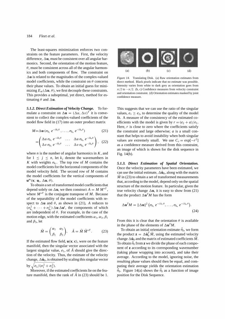
Finally Fig. 18 shows the detection and estimationof the motion bars in outdoor image sequence takenwith a hand-held camcorder. This sequence depictsa narrow tree (about 6 pixels wide) moving in frontof the ground plane. The difference in velocity is pre-dominantly horizontal, while the orientation of the treeis nearly vertical. Where the change in velocity be-tween the tree and ground is sufficiently large, towardsthe upper part of the tree, the moving bar is detectedwell.

Figure 17. Translating Annulus. (a) Frame 1 of sequence. (b) Recovered flow. (c) Confidence measureC from LS minimization. (d–f) Optimalestimates ofθ ,1u and1v whereC > 0.65.

5.2. Domain-Specific Experimental Results

In the case of generic motion features it was possible toevaluate the performance of the basis set with respect toan idealized optical flow model. In the case of domain-specific models such as human mouths, in which thebasis set is constructed from examples, no such ideal-ized models exist. Therefore, to evaluate the accuracyand stability of the motion estimated with these mod-els we consider the use of the recovered coefficients forthe task of recognition of motion events. This will helpdemonstrate that the recovered motion is a reasonablerepresentation of the true optical flow.

Below we consider domain specific models for hu-man mouths and legs and illustrate the use of the re-covered coefficients with examples of lip reading andwalking gait detection. These recognition tasks will


Figure 18. Small Tree Sequence. (a) Frame 1 of sequence. (b) Confidence measureC. (c–e) Optimal estimates ofθ , 1u and1v whereC > 0.65.

necessitate the construction of temporal models thatcapture the evolution of the coefficients over a numberof frames.

5.2.1. Non-Rigid Human Mouth Motion. Black andYacoob (1997) described a method for recognizing hu-man facial expressions from the coefficients of a pa-rameterized motion model. They modeled the face asa plane and used its motion to stabilize the image se-quence. The motion of the eyebrows and mouth wereestimated relative to this stabilized face using a sevenparameter model (affine plus a vertical curvature term).While this hand-coded model captures sufficient infor-mation about feature deformation to allow recognitionof facial expressions, it it does not capture the variabil-ity of human mouths observed in natural speech.

To test the accuracy and stability of the learned modelwe apply it the problem of lip reading for a simple userinterface called the Perceptual Browser (Black et al.,1998). The Perceptual Browser tracks the head of a hu-man sitting in front of a computer display and uses thesubject’s vertical head motion to control the scrollingof a window such as a web browser.

We explore the addition of four mouth “gestures” tocontrol the behavior of the browser:

• Center: mark the current head position as the “neu-tral” position.• Track: start tracking the head. In this mode the head

acts like a “joystick” and deviations from the neutralposition cause the page to scroll.• Release: stop head tracking. Head motions no lon-

ger cause scrolling.• Print: print the contents of the current page.

We think of these as “gestures” in that the user doesnot need to vocalize the commands but simply makesthe mouth motion associated with the words.

For training we used the 3000 image sequence de-scribed in Section 3.2.1 that contains the test utterancesas well as other natural speech and facial expressions.The head location was assumed to be known in the firstframe of the sequence and the head was tracked there-after using a planar motion model. The mouth locationrelative to the head was also known. The first three ba-sis vectors (with the largest eigenvalues) were used forestimating the motion; as discussed in Section 3.2.1,the mean flowf was not used as it accounts for signif-icantly less variance than the first three basis vectors.

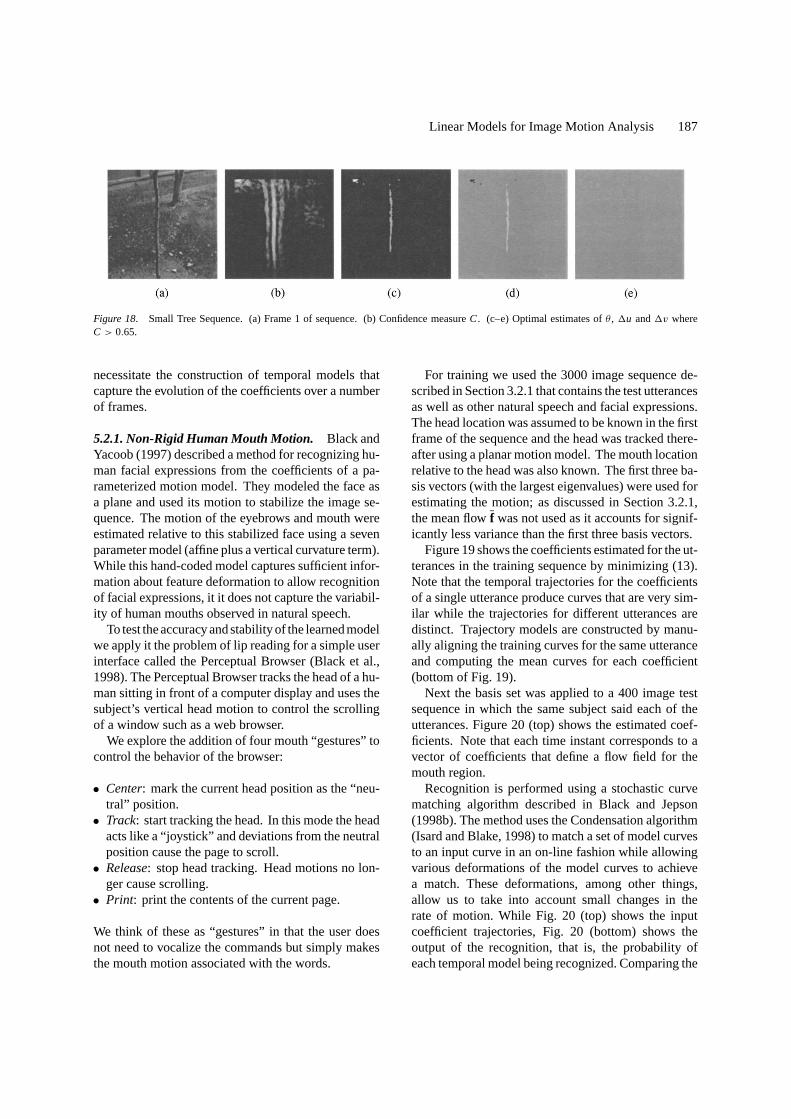
Figure 19 shows the coefficients estimated for the ut-terances in the training sequence by minimizing (13).Note that the temporal trajectories for the coefficientsof a single utterance produce curves that are very sim-ilar while the trajectories for different utterances aredistinct. Trajectory models are constructed by manu-ally aligning the training curves for the same utteranceand computing the mean curves for each coefficient(bottom of Fig. 19).

Next the basis set was applied to a 400 image testsequence in which the same subject said each of theutterances. Figure 20 (top) shows the estimated coef-ficients. Note that each time instant corresponds to avector of coefficients that define a flow field for themouth region.

Recognition is performed using a stochastic curvematching algorithm described in Black and Jepson(1998b). The method uses the Condensation algorithm(Isard and Blake, 1998) to match a set of model curvesto an input curve in an on-line fashion while allowingvarious deformations of the model curves to achievea match. These deformations, among other things,allow us to take into account small changes in therate of motion. While Fig. 20 (top) shows the inputcoefficient trajectories, Fig. 20 (bottom) shows theoutput of the recognition, that is, the probability ofeach temporal model being recognized. Comparing the

188 Fleet et al.

Figure 19. (Top) Example training sequences of mouth motion coefficients. (Bottom) Temporal models are constructed from the examples, toproduce model coefficient trajectories.

“spikes” in this plot with the input trajectories revealsthat the method recognizes the completion of each ofthe test utterances (see Black and Jepson (1998b) fordetails).

Further experimental work with linear parameter-ized models can be found in work on modeling ap-pearance changes in image sequences (Black et al.(2000)). In that work, linear parameterized motionmodels were used, in conjunction with models for othersources of appearance change in image sequences, toexplain image changes between frames in terms of amixture of causes (see Black et al. (2000) for moredetails).

5.2.2. Articulated Motion. Like mouths, the articu-lated motion of human limbs can be large, varied, anddifficult to model. Here we construct a view-basedmodel of leg motion and use it to recognize walkingmotions. We assume that the subject is viewed fromthe side (though the approach can be extended to cope

with other views) and that the image sequence has beenstabilized with respect to the torso. Two training andtwo test sequences (Fig. 21) of subjects walking on atreadmill were acquired with different lighting condi-tions, viewing position, clothing, and speed of activ-ity. One advantage of motion-based recognition overappearance-based approaches is that it is relatively in-sensitive to changes such as these.

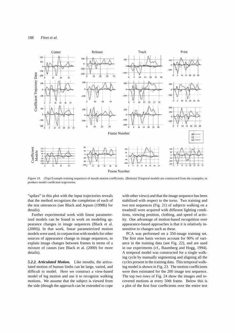
PCA was performed on a 350-image training set.The first nine basis vectors account for 90% of vari-ance in the training data (see Fig. 22), and are usedin our experiments (cf., Baumberg and Hogg, 1994).A temporal model was constructed for a single walk-ing cycle by manually segmenting and aligning all thecycles present in the training data. This temporal walk-ing model is shown in Fig. 23. The motion coefficientswere then estimated for the 200 image test sequence.The top two rows of Fig. 24 show the images and re-covered motions at every 50th frame. Below this isa plot of the first four coefficients over the entire test


Figure 20. Word detection from mouth motion coefficients: (Top) With a test sequence, the model coefficients are estimated between everypair of frames. For the mouth model we used 3 basis flow fields, the coefficients of which are shown for a 400 frame test sequence. (Bottom)Recognition probabilities for test words from the mouth motion (see text).

Figure 21. Articulated human motion. The first two images arefrom the training sequences, and the second two are from test se-quences.

sequence. The Condensation-based recognition algo-rithm was used to recognize the walking cycles. Thepeaks in the bottom plot in Fig. 24 correspond to thedetection of a completed walking cycle.

6. Conclusion

Linear parameterized motion models can provide effec-tive descriptions of optical flow. They impose strongconstraints on the spatial variation of the optical flow

within an image region and they provide a concise de-scription of the motion in terms of a small number oflinear coefficients. Moreover, the model coefficientscan be estimated directly from the image derivativesand do not require the prior computation of dense im-age motion. The framework described here extendsparameterized flow methods to more complex motions.

We have explored the use of linear parameterizedmodels to represent generic, discontinuous motion fea-tures including occlusion boundaries and motion bars.The models are applied at every image location in theway that current affine models are employed, and themodel coefficients are estimated from the image in ex-actly the same way as affine motion coefficients arecomputed, with robust, coarse-to-fine optical flow tech-niques. Finally, we have shown how to reliably detectthe presence of a motion feature from the linear coeffi-cients and how to recover the feature orientation and therelative velocities of the surfaces. This work shows oneway to extend regression-based optical flow methods

190 Fleet et al.

Figure 22. Basis flow fields for the walking sequences.

Figure 23. Temporal trajectory model for walking.

to cope with more complex features and helps bringto light the relationships between static image featuresand motion features. We have also used this method asa means for initializing a particle filter for detecting andtracking motion boundaries with a higher-dimensionalnonlinear model (Black and Fleet, 1999).

The framework presented here also extends linearparameterized motion models to object-specific do-mains (e.g., mouth motion or human walking motions).In these domains, rather than explicitly constructing themodel bases, we learn them from sets of training flowfields. Principal component analysis is used to con-struct low-dimensional representations of the motionclasses, the coefficients of which are estimated directlyfrom spatiotemporal image derivatives. Unlike the mo-tion features above, we have applied these models inspecific image regions. For example, once a head istracked and stabilized the motion of the mouth canbe estimated using the learned mouth motion model.This model alignment in the image is important, andit may be possible to refine this alignment automat-

Figure 24. Top two rows: images and estimated flow for every 50thframe in the test sequence. Third row: Plot of the first four motioncoefficients for one test sequence. Bottom row: Plot showing thedetection of completed walking cycles.

ically (see Black and Jepson, 1998a). The temporalbehaviour of the model coefficients then provide a richdescription of the local motion information. To showthis, we have used the time-varying behaviour of thecoefficients to construct and recognize various simpletemporal “gestures” (Black and Jepson, 1998b). Theseinclude spoken words with mouth motion, and a walk-ing gait in the context of human locomotion. Speech


recognition from lip motion alone is of course a verychallenging task and we have demonstrated results ina highly constrained domain. Future work should ex-plore the combination of motion with appearance in-formation and audio.

Future Work

In future work we plan to extend the use of linear pa-rameterized models in several ways. With motion fea-tures we plan to improve the detection method with thecombined (edge and bar) basis set to use the coeffi-cient behavior in both subspaces to improve detectionand parameter estimation. We expect that localizationcan be greatly improved in this way. Localization canbe further improved with the inclusion of informationabout static image features, because motion edges oftencoincide with intensity edges.

A related issue concerns the fact that we have onlyused motion features at a single scale. As one conse-quence of this, we do not currently detect bars muchwider than 8 or 10 pixels, and we do not estimate thewidth of the bar. It may be desirable to have edge andbar models at a variety of scales that provide better spa-tial resolution at fine scales and potentially better de-tection at coarser scales. In this case we would expectthat structure could be tracked through scale, where,for example, two edges at one scale would be detectedas a bar at a coarser scale. Another way to includemultiple scales would be to use a multiscale waveletbasis to represent optical flow (Wu et al., 1998). Fromthe wavelet coefficients one could detect motion edgesand bars much like intensity edges are detected fromimage wavelet transforms.

Currently, the coefficients of each image region areestimated independently and it would be interesting toexplore the regularization of neighboring coefficientsto reduce noise and enforce continuity along contours.However, the exploitation of statistical dependencesbetween events in nearby regions may be best incorpo-rated at a subsequent stage of analysis, like the proba-bilitic approach described in Black and Fleet (1999).

With the domain-specific motion models, we as-sumed that we were given the appropriate image lo-cation within which to apply the models. If size andshape of the actual image region is somewhat differentfrom training set, then one might also allow an affinedeformation to warp the image data into the subspace(cf., Black and Jepson, 1998a). More generally, givena set of models that characterize a variety of motions in

the natural world, we would like to find the appropriatemodel to use in a given region; this is related to work onobject and feature recognition using appearance basedmodels (Nayar et al., 1996).

A number of other research issues remain unan-swered. Learned models are particularly useful in sit-uations where optical flow is hard to estimate, but inthese situations it is difficult to compute reliable train-ing data. This problem is compounded by the sensi-tivity of PCA to outliers. PCA also gives more weightto large motions making it difficult to learn compactmodels of motions with important structure at multi-ple scales. Future work will explore non-linear modelsof image motion, robust and incremental learning, andmodels of motion texture.

Acknowledgments

We are grateful to Prof. Mubarak Shah for suggestingto us the application of PCA to optical flow fields. DJFwas supported by NSERC Canada and by an Alfred P.Sloan Research Fellowship.

References

Ayer, S. and Sawhney, H. 1995. Layered representation of motionvideo using robust maximum-likelihood estimation of mixturemodels and MDL encoding. InProc. IEEE International Con-ference on Computer Vision, Boston, MA, pp. 777–784.

Bab-Hadiashar, A. and Suter, D. 1998. Robust optical flow compu-tation.International Journal of Computer Vision, 29:59–77.

Barron, J.L., Fleet, D.J., and Beauchemin, S.S. 1994. Performance ofoptical flow techniques.International Journal of Computer Vision,12(1):43–77.

Baumberg, A. and Hogg, D. 1994. Learning flexible models fromimage sequences. InProc. European Conf. on Computer Vision,Stockholm, Sweden, J. Eklundh, (Ed.), LNCS-Series, Vol. 800,Springer-Verlag, pp. 299–308.

Beauchemin, S.S. and Barron, J.L. (2000). The local frequency struc-ture of 1d occluding image signals.IEEE Transactions on PatternAnalysis and Machine Intelligence, 22(3).

Bell, A.J. and Sejnowski, T.J. 1997. The independent componentsof natural scenes are edge filters.Vision Research, 37(23):3327–3338.

Bergen, J.R., Anandan, P., Hanna, K., and Hingorani, R. 1992a.Hierarchical model-based motion estimation. InProc. EuropeanConf. on Comp. Vis., Springer-Verlag, pp. 237–252.

Bergen, J.R., Burt, P.J., Hingorani, R., and Peleg, S. 1992b. A three-frame algorithm for estimating two-component image motion.IEEE Transactions on Pattern Analysis and Machine Intelligence,14(9):886–896.

Beymer, D. 1996. Feature correspondence by interleaving shape andtexture computations. InProc. IEEE Computer Vision and PatternRecognition, San Francisco, pp. 921–928.

192 Fleet et al.

Black, M., Berard, F., Jepson, A., Newman, W., Saund, E., Socher,G., and Taylor, M. 1998. The digital office: Overview. InAAAISpring Symposium on Intelligent Environments, Stanford, CA,pp. 1–6.

Black, M.J. and Anandan, P. 1990. Constraints for the early detectionof discontinuity from motion. InProc. National Conf. on ArtificialIntelligence, AAAI-90, Boston, MA, pp. 1060–1066.

Black, M.J. and Anandan, P. 1996. The robust estimation of multiplemotions: Parametric and piecewise-smooth flow fields.ComputerVision and Image Understanding, 63(1):75–104.

Black, M.J. and Jepson, A.D. 1998a. EigenTracking: Robust match-ing and tracking of articulated objects using a view-based repre-sentation.International Journal of Computer Vision, 26(1):63–84.

Black, M.J. and Jepson, A.D. 1998b. A probabilistic framework formatching temporal trajectories: Condensation-based recognitionof gestures and expressions. InProc. European Conf. on ComputerVision, H. Burkhardt and B. Neumann (Eds.), Freiburg, Germany,LNCS-Series, Vol. 1406, Springer-Verlag, pp. 909–924.

Black, M.J. and Yacoob, Y. 1997. Recognizing facial expressionsin image sequences using local parameterized models of imagemotion.International Journal of Computer Vision, 25(1):23–48.

Black, M.J., Yacoob, Y., Jepson, A.D., and Fleet, D.J. 1997. Learningparameterized models of image motion. InProc. IEEE ComputerVision and Pattern Recognition, Puerto Rico, pp. 561–567.

Black, M.J. and Fleet, D.J. 1999. Probabilistic detection and trackingof motion discontinuities. InProc. IEEE International Conferenceon Computer Vision, Corfu, Greece, pp. 551–558.

Black, M.J., Fleet, D.J., and Yacoob, Y. (2000). Robustly estimat-ing changes in image appearance.Computer Vision and ImageUnderstanding, 78(1):8–31.

Bregler, C. and Malik, J. 1998. Tracking people with twists andexponential maps. InProc. IEEE Computer Vision and PatternRecognition, Santa Barbara, pp. 8–15.

Bregler, C. and Omohundro, S.M. 1995. Nonlinear manifold learn-ing for visual speech recognition. InProc. IEEE InternationalConference on Computer Vision, Boston, MA, pp. 494–499.

Burt, P.J., Bergen, J.R., Hingorani, R., Kolczynski, R., Lee, W.A.,Leung, A., Lubin, J., and Shvaytser, H. 1989. Object tracking witha moving camera: An application of dynamic motion analysis. InProc. IEEE Workshop on Visual Motion, Irvine, CA, pp. 2–12.

Chou, G.T. 1995. A model of figure-ground segregation from kineticocclusion. InProc. IEEE International Conference on ComputerVision, Boston, MA, pp. 1050–1057.

Cootes, T.F., Edwards, G.J., and Taylor, C.J. 1995. Active ap-pearance models. InProc. European Conf. on Computer Vision,H. Burkhardt and B. Neumann (Eds.), Freiburg, Germany, LNCS-Series, Vol. 1406, Springer-Verlag, pp. 484–498.

Darrell, T. and Pentland, A. 1995. Cooperative robust estimationusing layers of support.IEEE Transactions on Pattern Analysisand Machine Intelligence, 17(5):474–487.

Ezzat, T. and Poggio, T. 1996. Facial analysis and synthesis us-ing image-based models. InProc. International Conference onAutomatic Face and Gesture Recognition, Killington, Vermont,pp. 116–121.

Fennema, C.L. and Thompson, W.B. 1979. Velocity determinationin scenes containing several moving objects.Computer Vision,Graphics, and Image Processing, 9:301–315.

Fleet, D.J. and Jepson, A.D. 1990. Computation of component imagevelocity from local phase information.International Journal ofComputer Vision, 5:77–104.

Fleet, D.J. 1992. Measurement of Image Velocity. Kluwer AcademicPubl, Norwell.

Fleet, D.J. and Langley, K. 1994. Computational analysis of non-fourier motion.Vision Research, 22:3057–3079.

Freeman, W. and Adelson, E.H. 1991. The design and use of steer-able filters.IEEE Transactions on Pattern Analysis and MachineIntelligence, 13:891–906.

Geman, S. and McClure, D.E. 1987. Statistical methods for tomo-graphic image reconstruction.Bulletin of the International Statis-tical Institute, LII-4:5–21.

Golub, G.H. and van Loan, C.F. 1983.Matrix Computations. JohnsHopkins University Press: Baltimore, Maryland.

Hager, G. and Belhumeur, P. 1996. Real-time tracking of imageregions with changes in geometry and illumination. InProc. IEEEConference on Computer Vision and Pattern Recognition, SanFrancisco, CA, pp. 403–410.

Hallinan, P. 1995. A deformable model for the recognition of humanfaces under arbitrary illumination. Ph.D. Thesis, Harvard Univer-sity, Cambridge, MA.

Harris, J.G., Koch, C., Staats, E., and Luo, J. 1990. Analog hardwarefor detecting discontinuities in early vision.Int. Journal of Comp.Vision, 4(3):211–223.

Heitz, F. and Bouthemy, P. 1993. Multimodal motion estima-tion of discontinuous optical flow using markov random fields.IEEE Transactions on Pattern Analysis and Machine Intelligence,15(12):1217–1232.

Isard, M. and Blake, A. 1998. Condensation—conditional densitypropagation for visual tracking.International Journal of ComputerVision, 29(1):2–28.

Jepson, A. and Black, M.J. 1993. Mixture models for optical flowcomputation. InPartitioning Data Sets: With Applications to Psy-chology, Vision and Target Tracking, Ingmer Cox, Pierre Hansen,and Bela Julesz (Eds.), AMS Pub.: Providence, RI, pp. 271–286.DIMACS Workshop.

Ju, S.X., Black, M.J., and Jepson, A.D. 1996. Skin and bones:Multi-layer, locally affine, optical flow and regularization withtransparency. InProc. IEEE Conference on Computer Vision andPattern Recognition, San Francisco, pp. 307–314.

Kearney, J.K. and Thompson, W.B. 1987. An error analysis of gra-dient-based methods for optical flow estimation.IEEE PatternAnalysis and Machine Intelligence, 19(2):229–244.

Lucas, B.D. and Kanade, T. 1981. An iterative image registrationtechnique with an application to stereo vision. InProc. Inter-national Joint Conference on Artificial Intelligence, Vancouver,pp. 674–679.

Nastar, C., Moghaddam, B., and Pentland, A. 1996. Generalized im-age matching: Statistical learning of physically-based deforma-tions. InProc. European Conf. on Computer Vision, Cambridge,UK, B. Buxton and R. Cipolla (Eds.), LNCS-Series, Vol. 1064,Springer-Verlag, pp. 589–598.

Nayar, S.K., Baker, S., and Murase, H. 1996. Parametric fea-ture detection. InProc. IEEE Conference on Computer Visionand Pattern Recognition, San Francisco, CA. IEEE, pp. 471–477.

Nelson, R.C. and Polana, R. 1992. Qualitative recognition of motionusing temporal texture.CVGIP: Image Understanding, 56(1):78–89.

Niyogi, S.A. 1995. Detecting kinetic occlusion. InProc. IEEEInternational Conference on Computer Vision, Boston, MA,pp. 1044–1049.


Ong, E.P. and Spann, M. 1999. Robust optical flow computationbased on least-median-of-squares regression.International Jour-nal of Computer Vision, 31:51–82.

Perona, P. 1995. Deformable kernels for early vision.IEEE Transac-tions on Pattern Analysis and Machine Intelligence, 17:488–499.

Potter, J.L. 1980. Scene segmentation using motion information.IEEE Trans. S.M.C., 5:390–394.

Sclaroff, S. and Isidoro, J. 1998. Active blobs. InProc. Interna-tional Conference on Computer Vision, Mumbai, India, pp. 1146–1153.

Sclaroff, S. and Pentland, A.P. 1994. Physically-based combinationsof views: Representing rigid and nonrigid motion. InProceedingsof the Workshop on Motion of Non-rigid and Articulated Objects,Austin, Texas, pp. 158–164.

Shulman, D. and Herve, J.Y. 1989. Regularization of discontinuousflow fields. InProc. IEEE Workshop on Visual Motion, Irvine, CA,pp. 81–86.

Spoerri, A. and Ullman, S. 1987. The early detection of motionboundaries. InProc. IEEE International Conference on ComputerVision, London, UK, pp. 209–218.

Szeliski, R. and Coughlan, J. 1997. Spline-based image registration.International Journal of Computer Vision, 22:199–213.

Szeliski, R. and Shum, H. 1996. Motion estimation with quadtreesplines.IEEE Transactions on Pattern Analysis and Machine In-telligence, 18(12):1199–1211.

Thompson, W.B., Mutch, K.M., and Berzins, V.A. 1985. Dynamicocclusion analysis in optical flow fields.IEEE Transactions onPattern Analysis and Machine Intelligence, 7:374–383.

Vasconcelos, N. and Lippman, A. 1998. A spatiotemporal mo-tion model for video summerization. InProc. IEEE Conference

on Computer Vision and Pattern Recognition, Santa Barbara,pp. 361–366.

Vetter, T. 1996. Learning novel views to a single face image. InProc. International Conference on Automatic Face and GestureRecognition, Killington, Vermont, pp. 22–27.

Vetter, T., Jones, M.J., and Poggio, T. 1997. A bootstrapping algo-rithm for learning linear models of object classes. InProc. IEEEConference on Computer Vision and Pattern Recognition, PuertoRico, pp. 40–46.

Wang, J.Y.A. and Adelson, E.H. 1994. Representing moving imageswith layers.IEEE Transactions on Image Processing, 3(5):625–638.

Waxman, A.M. and Wohn, K. 1985. Contour evolution, neighbour-hood deformation and global image flow: Planar surfaces in mo-tion. International Journal of Robotics Research, 4:95–108.

Weiss, Y. 1997. Smoothness in layers: Motion segmentation usingnonparametric mixture estimation. InProc. IEEE Conference onComputer Vision and Pattern Recognition, Puerto Rico, pp. 520–526.

Weiss, Y. and Adelson, E.H. 1996. A unified mixture framework formotion segmentation: Incorporating spatial coherence and esti-mating the number of models. InProc. IEEE Computer Visionand Pattern Recognition, San Francisco, pp. 321–326.

Wu, Y., Kanade, T., Cohn, J., and Li, C. 1998. Optical flow esti-mation using wavelet motion model. InProc. IEEE InternationalConference on Computer Vision, Mumbai, India, pp. 992–998.

Yamamoto, M., Sato, S., Kuwada, S., Kondo, T., and Osaki, Y.1998. Incremental tracking of human actions from multiple views.In Proc. IEEE Computer Vision and Pattern Recognition, SantaBarbara, pp. 2–7.

design and use of linear models for image motion analysisjepson/papers/fleetblackyacoob... ·...

Documents