design and optimization of annular flow electromagnetic

Research ArticleDesign and Optimization of Annular Flow ElectromagneticMeasurement System for Drilling Engineering

Liang Ge ,1,2,3 Hailong Li,2 Qing Wang,3 Guohui Wei,2 Ze Hu,2 Junbi Liao,1 and Junlan Li4

1School of Manufacturing Science and Engineering, Sichuan University, Chengdu 610065, China2College of Mechanical and Electronic Engineering, Southwest Petroleum University, Chengdu 610500, China3Department of Engineering, Durham University, Durham DH1 3LE, UK4Southwest Branch, Engineering Design Co., CNPC, Chengdu 610413, China

Correspondence should be addressed to Liang Ge; [email protected]

Received 28 June 2017; Accepted 18 October 2017; Published 25 February 2018

Academic Editor: Bruno Andò

Copyright © 2018 Liang Ge et al. This is an open access article distributed under the Creative Commons Attribution License, whichpermits unrestricted use, distribution, and reproduction in any medium, provided the original work is properly cited.

Using the downhole annular flow measurement system to get real-time information of downhole annular flow is the core andfoundation of downhole microflux control drilling technology. The research work of electromagnetic flowmeter in recent yearscreates a challenge to the design of downhole annular flow measurement. This paper proposes a design and optimization ofannular flow electromagnetic measurement system for drilling engineering based on the finite element method. Firstly, theannular flow measuring and optimization principle are described. Secondly, a simulation model of an annular flowelectromagnetic measurement system with two pairs of coil is built based on the fundamental equation of electromagneticflowmeter by COMSOL. Thirdly, simulations of the structure of excitation system of the measurement system are carried out,and simulations of the size of the electrode’s radius are also carried out based on the optimized structure, and then all thesimulation results are analyzed to evaluate the optimization effect based on the evaluation indexes. The simulation results showthat optimized shapes of the excitation system and electrode size can yield a better performance in the annular flow measurement.

1. Introduction

In recent decades, oil and gas exploration is being carried outin some extremely harsh and challenging environmentalconditions [1]. Drilling safety issues become increasinglyprominent when exploring complex and deep formations.Downhole microflux control drilling technology can effec-tively solve drilling accident such as kick and lose in narrowdensity window drilling scenarios, so using the measurementsystem to get the real-time information of downhole annularflow is the core and foundation of downhole microflux con-trol drilling technology.

A huge array of flow technology options is on offer whichprovides options in selecting the correct annular flow mea-surement for the application of drilling engineering. A broadrange of factors regarding the special environment of down-hole drilling, such as downhole space, velocity profile,

temperature, and fluid properties, should be considered.Electromagnetic measurement has the advantages of simplestructure, no moving parts, and no obstruction of fluid flowthrottle parts. Also, the flow path does not cause any addi-tional pressure loss, and it does not cause wear or blockage,in particular when measuring slurry with solid particles, sew-age and other liquid-solid two-phase bodies, or a variety ofviscous slurry, and so on. In addition, because the structurehas no moving parts, so any corrosion will be attached tothe insulation lining. After selecting corrosion-resistant elec-trode material with a very good corrosion resistance, it can beused for a variety of corrosive media measurements. In 2017,Liang et al. propose a new method for an annular flow mea-surement system based on the electromagnetic inductionprinciple [2]. However, this paper does not describe how todesign and optimize the downhole annular flow electromag-netic measurement system. Based on the above reasons, this

HindawiJournal of SensorsVolume 2018, Article ID 4645878, 12 pageshttps://doi.org/10.1155/2018/4645878

http://orcid.org/0000-0003-4549-6946

https://doi.org/10.1155/2018/4645878

study mainly focuses on the design and optimization ofdownhole annular flow electromagnetic measurement sys-tem for drilling engineering.

For the traditional electromagnetic flowmeter used in around pipe, the signal voltage is dependent on the averageflow velocity, the magnetic flux density, and the pipe diame-ter. The signal voltage is expected to be linearly related to theaverage flow velocity if the magnetic field is a uniform mag-netic field. In this ideal case, the flow rate can be consideredto be immune to the velocity profile of the pipe flow, espe-cially when the flow has been fully developed. However, itis difficult for the annular flow electromagnetic measurementsystem to yield a uniform magnetic field for an annular flowpath, and also, the velocity profile of the annular flow alsocannot be considered axisymmetrically distributed under thisspecial drilling environment. These effects affect the accuracyof the annular flow electromagnetic measurement system.According to Bevie’s vector weight function theory [3], ifthe result of the magnetic flux density cross-product densityof virtual current is constant, the annular flow electromag-netic measurement system can be considered to be immuneto the velocity profile of the annular flow.When the electrodeand the structure of the flow path are fixed, the density of thevirtual current is fixed. So the shape of the excitation systemcan be derived based on this constant condition. Similarly,when the shape of excitation system and the structure of flowpath are fixed, the density of virtual current only depends onthe electrodes. In this case, the size of the electrode wasselected to be optimized to reduce the distortion caused bythe velocity profile.

In the past few decades, great efforts about the structureof excitation systems and electrodes have been made toreduce the effects of the velocity profile. Horner B improvedthe measurement accuracy of flow measurement byincreasing the number of electrodes [4, 5]. Michalski et al.investigated the design of the coils of an electromagneticflowmeter in 1998 [6]. Wang et al. analyzed the relationshipbetween velocity profile and distribution of induced potentialfor an electromagnetic flow meter in 2007 [7]. An optimumexcitation coil for an open channel electromagnetic flowme-ter was reported by Michalski et al. in 2001 [8]. Vieira et al.developed an enhanced ellipsoid method for electromagneticdevice optimization and design in 2010 [9]. At the same time,some simulation methods were designed with the develop-ment of finite element software for multifields. Lim andChoong analyzed the relative errors in evaluating the electro-magnetic flowmeter signal using the weight function methodand the finite volume method [10]. Michalski et al. applied3D approach to designing the excitation coil of an electro-magnetic flowmeter in 2012 [11]. Yin et al. investigated thetheoretical and numerical approaches to the sensitivity calcu-lation of a novel contactless inductive flow tomography [12].Although great efforts about the structure of the excitationsystem and electrodes have been made to reduce the effectsof velocity profile, most of the design and optimization wasfocused on the round pipe. The main objective of this paperis to design and optimize the downhole annular flow electro-magnetic measurement system with two pairs of electrodesusing the method of numerical finite element analysis.

2. Background Theory of the Annular Four-Electrode Electromagnetic Flowmeter

Following Faraday’s law, the flow of a conductive liquidthrough a magnetic field will cause a voltage signal to besensed by electrodes located on the flow pipe walls. Faraday’sformula can be expressed as

E = BDv, 1

where E is the signal voltage in a conductor, v is the aver-age flow velocity, B is the magnetic flux density, and D is thepipe diameter.

Equation (1) indicates that the signal voltage is depen-dent on the average flow velocity, the magnetic flux density,and the pipe diameter.

The signal voltage is expected to be linearly related to theaverage flow velocity if the magnetic field is a uniform mag-netic field. So (1) can be rewritten as

E = Cv 2

Here, C represents a constant.However, the annular flow electromagnetic measurement

system is difficult to yield a uniform magnetic field for anannular flow path, and the velocity profile of the annular flowalso cannot be considered axisymmetrically distributedunder this special drilling environment. This affects theaccuracy of the annular flow electromagnetic measurementsystem. So the design and optimization of the downholeannular flow electromagnetic measurement system withtwo pairs of electrodes cannot be investigated based on thetraditional Faraday theory.

According to Bevir’s theory [3], the theoretical expres-sion of the induced potential in annular flow electromag-netic measurement system can be given as a volumeintegral of the weight function vector W and the annularflow velocity ν as follows:

U =τ

W ⋅ v d τ, 3

where W is given by W = B × j .Here,U is the induced potential,W is the weight function

vector, ν is the velocity of the annular flow, B is the mag-

netic flux vector, j is the virtual current vector, and τ isthe integration of annular volume. The velocity of the annu-lar flow weight function vector W is dependent on the mag-

netic flux density vector B and virtual current vector j .According to Bevie’s vector weight function theory, if the

result of the magnetic flux density cross-product density ofvirtual current is constant, the annular flow electromagneticmeasurement system can be considered to be immune tothe velocity profile of the annular flow. When the electrodeand the structure of the flow path are fixed, the density of vir-tual current is fixed. Thus, the shape of excitation system canbe derived based on this constant condition. Similarly, whenthe shape of the excitation system and the structure of the

2 Journal of Sensors

flow path are fixed, the density of the virtual current onlydepends on the electrodes. In this case, the radius of the elec-trode was selected to be optimized to reduce the distortioncaused by the velocity profile.

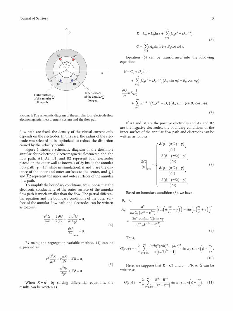
Figure 1 shows a schematic diagram of the downholeannular four-electrode electromagnetic flowmeter and theflow path. A1, A2, B1, and B2 represent four electrodesplaced on the outer wall at intervals of 2γ inside the annularflow path (γ = 45° while in simulation), a and b are the dis-tance of the inner and outer surfaces to the center, and ∑1and ∑2 represent the inner and outer surfaces of the annularflow path.

To simplify the boundary conditions, we suppose that theelectronic conductivity of the outer surface of the annularflow path is much smaller than the flow. The partial differen-tial equation and the boundary conditions of the outer sur-face of the annular flow path and electrodes can be writtenas follows:

∂2G∂r2

+ 1r∂G∂r

+ 1r2∂2G∂ϕ2

= 0,

∂G∂r r=b

= 04

By using the segregation variable method, (4) can beexpressed as

r2d2R

dr2+ r

dRdr

− KR = 0,

d2Φdϕ2

+ Kϕ = 05

When K = n2, by solving differential equations, theresults can be written as

R = C0 +D0ln r + 〠∞

n=1Cnr

n +Dnr−n ,

Φ = 〠∞

n=1Ansin nϕ + Bncos nϕ

6

Equation (6) can be transformed into the followingequation:

G = C0 +D0ln r

+ 〠∞

n=1Cnr

n +Dnr−n An sin nϕ + Bn cos nϕ ,

∂G∂r

=D01r

+ 〠∞

n=1nr−n−1 Cnr

2n −Dn An sin nϕ + Bn cos nϕ

7

If A1 and B1 are the positive electrodes and A2 and B2are the negative electrodes, the boundary conditions of theinner surface of the annular flow path and electrodes can bewritten as follows:

∂G∂r r=a

=

δ ϕ − π/2 + γ

2a ,

−δ ϕ − π/2 − γ

2a ,

δ ϕ + π/2 + γ

2a ,

−δ ϕ + π/2 − γ

2a

8

Based on boundary condition (8), we have

Bn = 0,

An =an

nπCn a2n − b2nsin n

π

2 − γ − sin nπ

2 + γ

= −2an cos nπ/2 sin nγ

nπCn a2n − b2n

9

Thus,

G r, ϕ = −2π

〠∞

n=2,4,6

a/b n r/b n + a/r n

n a/b 2n − 1sin nγ sin n ϕ + π

210

Here, we suppose that R = r/b and τ = a/b, so G can bewritten as

G r, ϕ = −2π

〠∞

n=2,4,6

Rn + R−n

n τn − τ−nsin nγ sin n ϕ + π

2 11

A1

B2

a

b

X

Y

∑∑

A2

B1

2𝛾

Outer surfaceof the annular

flowpath

Inner surfaceof the annular

flowpath2 1

Figure 1: The schematic diagram of the annular four-electrode flowelectromagnetic measurement system and the flow path.

3Journal of Sensors

The density of the virtual current can be derived using thegradient method based on (11). Theoretically, the shape andthe parameters of the exciting coil can be solved based on theconstant condition of the weight function vector. However, itis very complicated and difficult to derive the shape and theparameters of the exciting coil by the analytical method. Evenif the result is solved, it is also complicated and difficult forthe coil to wind. In recent years, numerical simulation hasbecome an important process in a new system design. Thesedifficulties can be worked out by the finite element softwarefor multifields.

3. Optimization of the Annular Four-ElectrodeElectromagnetic Flowmeter

3.1. Optimization of Excitation Structure. To avoid windingthe complicated coil, the iron core was introduced to theexcitation part of the annular flow electromagnetic measure-ment system. Considering the special downhole environ-ment, the schematic diagram of the excitation part ofannular flow electromagnetic measurement system is shownin Figure 2. Here, the inner radius of the system is 4 cm, theouter radius is 9 cm, and the inner and outer wall thicknessof the system is 1 cm. In the annular flow electromagnetic

measurement system, four excitation coils were positionedto generate a magnetic field. Four pick-up electrodes werelocated around the diameter of the external system wall, sothat the flow-induced voltage could be detected. The 3Dmodel of the annular four-electrode flow electromagneticmeasurement system and the flow path by COMSOL areshown in Figure 3.

In this paper, the structure of the iron core and the size ofthe coil among the annular domain between the inner andouter surfaces of the system were investigated, and an opti-mized excitation structure was designed. Therefore, thewidth of the core and the height of core protrusion couldbe used as variables. In the simulations, the round electrodeswere chosen with a radius of 0.7 cm, and the length of theiron core was 10 cm. The excitation coils were modified withthe width of the core changing from 2 cm to 5 cm and theheight of core protrusion from 5.5 cm to 8.5 cm. The widthof the core was incremented every 1 cm, while the height ofcore protrusion every 1 cm.

To validate the effectiveness of the optimization, someperformances of the selected optimum annular flow electro-magnetic measurement system were compared. Comparedsimulation results of the magnetic flux vector and weightfunction vector are shown from Figures 4–7.

Figures 4–7 show that the distribution of the magneticflux vector and weight function vector changes with thewidth of the core and height of core protrusion changing.Considering the important role of weight function vector inoptimization, the weight function vector distributions fromFigures 4–7 are analyzed closely. The analysis results showthat the weight function vector gets the smallest distributionrange (from −0.03 to 0.32) when core_X is equal to 5.5 cmand Core_w is equal to 2 cm; the weight function vector getsthe biggest distribution range (from −0.05 to 0.66) whencore_X is equal to 8.5 cm and Core_w is equal to 5 cm; thedistribution range of the weight function vector increaseswhile the width of the core and height of core protrusionincrease steadily, and increasing the width of the coil is muchmore pronounced.

3.2. The Change of Electrode Radius. After the structure ofthe excitation system of the measurement system was opti-mized and in order to improve the accuracy of the system,some simulations about the radius of the electrodes wereused to improve the system performance. The electrodeswere modified, with the radius changing from 1 cm to5 cm, and the radius of the electrodes was incrementedevery 0.5 cm. Compared simulation results of the virtualcurrent vector and weight function vector are shown inFigures 8 and 9.

Figures 8 and 9 show that the virtual current density andweight function vector changed while the electrode radiuschanged. Based on Figures 8 and 9, we can find that theweight function vector gets the smallest distribution range(from 0 to 0.03) when the electrode radius is 5 cm; the weightfunction vector gets the biggest distribution range (from−0.01 to 0.16) when the electrode radius is 1 cm; the distribu-tion range of weight function vector decreases while the elec-trode radius increases steadily.

Iron core

Excitation coils

Electrode

Width of core

Height of coreprotrusion

Figure 2: The schematic diagram of the excitation part of theannular flow electromagnetic measurement system.

Figure 3: The 3D model of the annular four-electrode flowelectromagnetic measurement system and the flow path.


4. Results and Discussion

4.1. Evaluation Indexes

4.1.1. Standard Deviation of the Weight Function Vector. Theideal excitation system design is to make the weight functionvector to be a constant, and this is helpful to improve themeasurement accuracy of the system. However, the weightfunction vector is not easily designed to be a constant. Inorder to design a magnetic field that makes the weight func-tion vector as constant as possible, it is necessary to define adesign quantity that measures the degree of nonuniformityof the weight function vector over the cross-sectional areaof the annular domain. The definition of the design quantitywas discussed by Dennis and Wyatt in 1972 [13], but owingto integration difficulties, this quantity is not used here.Instead, a similar quantity Wσ named the weight function

vector standard deviation is used which is defined by thefollowing:

Wσ =〠N

i=1 Wi −W 2

N, 12

where W is the average weight function vector value of allpoints in the XY plane of the annular while z=0 and N isthe number of the points.

4.1.2. Homogeneity Range Ratio of Weight Function Vector.To evaluate the homogeneity range in the annular area,the ratio of the homogeneity range is used as an evalua-tion criterion [14]. The equation of this evaluation criterionis as follows:

1416

0.320.310.30.290.270.260.250.230.220.210.190.180.170.160.140.130.120.10.090.080.070.050.040.03

−0.03

0.01−0.010

×10−2

14

12

1

0.8

0.6

0.4

0.2

1210

86420

−2−4−6−8−10

−10 −5 0 5 10

−12−14

141210

86420

−2−4−6−8−10

−10 −5 0 5 10

−12−14

(a) When the height of core protrusion is 5.5 cm

0.340.330.310.30.290.270.260.240.230.220.20.190.180.160.150.140.120.110.10.080.070.050.040.03

−0.030.01−0.01

×10−3

148

7

6

5

4

3

2

1

1210

86420

−2−4−6−8−10−12−14

141210

86420

−2−4−6−8−10−12−14

−10 −5 0 5 10 −10 −5 0 5 10

(b) When the height of core protrusion is 7.5 cm

Figure 4: The simulation diagram of the magnetic flux vector and weight function vector with core width equal to 2 cm.

5Journal of Sensors

W x,y −WW × 100% ≤ P, 13

where W x,y is the weight function vector of the centralcross section of the electrode in the annular area, W is theaverage weight function vector value of all points in theXY plane of the annular while z=0, and P is a uniformpercentage value that depends on actual distribution andwhich is 30% in this research.

If a finite element meets (13), we may regard the area ofthis finite element to be homogeneous; otherwise, we regardthat the area of this finite element is inhomogeneous. If thenumber of inhomogeneous finite elements is N1 and thenumber of homogeneous finite elements is N2, the homoge-neity range ratio can be defined as follows:

Pe =N2

N1 +N2× 100% 14

4.1.3. The Coefficient of Variation of Weight Function Vector.The coefficient of variation is a useful statistic for comparingthe degree of variation from one data series to another, evenif the means are drastically different from one another. Acoefficient of variation of the weight function vector is a sta-tistical measure of the dispersion of the weight function

vector data points in a data series around the mean. It iscalculated as follows:

Cv =Wσ

W , 15

where Wσ is the standard deviation of the weight functionvector and W is the average weight function vector value ofall points.

4.1.4. The Sensitivity of Output Voltage. The fourth perfor-mance criterion is the sensitivity of the output voltage whichgives the strength of the system output. In this research, weassure that the turns and current of the coil are constant,and we get the sensitivity of the output voltage while the aver-age flow velocity is 1 meter per second.

During the optimal design and quantitative evaluationprocess, smaller standard deviation of the weight functionvector is better, as is a bigger homogeneity range ratio ofthe weight function vector is better, smaller coefficient ofvariation of the weight function vector is better, and biggersensitivity of the output voltage is better. In these four evalu-ation indexes, the standard deviation of the vector weightfunction is the most important evaluation index, and theother 3 indexes are auxiliary reference indexes.

141210

86420

−2−4−6−8−10

−20

×10−2

1

0.8

0.6

0.4

0.2

−15 −10 −5 0 5 10 15 20

−12−14

141210

86420

−2−4−6−8−10

−20 −15 −10 −5 0 5 10 15 20

−12−14

0.410.390.360.340.330.310.30.280.260.250.230.210.20.180.160.150.130.120.10.080.070.050.030.020−0.01−0.03


141210

86420

−2−4−6−8−10

−20

×10−3

5

4

3

2

1

−15 −10 −5 0 5 10 15 20

−12−14

141210

86420

−2−4−6−8−10

−20 −15 −10 −5 0 5 10 15 20

−12−14

0.430.420.40.380.360.350.330.310.30.260.240.28

0.230.210.190.170.160.140.120.110.090.070.050.040.020−0.02−0.03




×10−3

9

8

7

6

5

4

3

2

1

−20 −15 −10 −5 0 5 10 15 20

14121086420

−2−4−6−8−10−12−14

14121086420

−2−4−6−8−10−12−14

−20 −15 −10 −5 0 5 10 15 20

0.510.490.470.450.430.410.390.37

0.310.290.330.35

0.270.250.220.20.180.160.140.120.10.080.060.040.020−0.02−0.04


×10−3

8

7

6

5

4

3

2

1

−20 −15 −10 −5 −20 −15 −10 −50 5 10 15 20

14121086420

−2−4−6−8−10−12−14

0 5 10 15 20

14121086420

−2−4−6−8−10−12−14

0.540.520.50.470.450.430.410.39

0.320.350.3

0.37

0.280.260.240.220.20.170.150.110.090.070.050.020−0.02−0.04



14121086420

−2−4−6−8−10

−20 −15 −10 −5 −20 −15 −10 −50 5 10 15 20

70.620.590.570.540.520.50.470.450.420.40.370.350.320.30.280.250.230.20.180.150.130.10.080.060.030.01−0.02−0.04

×10−3

6

5

4

3

2

1−12−14

14121086420

−2−4−6−8−10

0 5 10 15 20

−12−14


0.660.630.610.580.550.530.50.480.450.420.40.370.340.320.290.270.240.210.190.160.140.110.080.060.030.01−0.02−0.04

×10−3

4.5

4

3.5

3

2.5

2

1.5

0.5

1

14121086420

−2−4−6−8−10

−20 −15 −10 −5 −20 −15 −10 −50 5 10 15 20

−12−14

−2−4−6−8−10−12−14

14121086420

0 5 10 15 20



7Journal of Sensors

4.2. Analysis of the Excitation System Optimization Effect. Inorder to intuitively analyze and compare the effect of excita-tion structure optimization, the value of the weight functionvector standard deviation is analyzed by the definition ofthe design quantity. To validate the effectiveness of the opti-mization, the results of the weight function vector standarddeviation are compared in Figure 10.

In Figure 10, Core_w represents the width of the core andcore_X represents the height of core protrusion. When thewidth of the core is fixed, the weight function vector standarddeviation increases while the height of core protrusionincreases steadily. When the height of core protrusion is

fixed, the weight function vector standard deviation increaseswhile the position of the width of the core increases steadily.

Using Figure 10, we can find the minimum standarddeviation of the weight function vector while core_X is5.5 cm and Core_w is 2 cm. Similarly, based on the simula-tion data and mathematical operations, the variation curveof the homogeneity range ratio, coefficient of variation ofthe weight function vector, and the sensitivity of the outputvoltage are shown from Figures 11–13.

It can be seen from Figures 11–13 that when the width ofthe core and height of core protrusion change, the evaluationindexes change. When core_X is equal to 5.5 cm and Core_w

14 1.05×103

1.010.970.930.890.850.810.770.740.70.660.620.580.540.50.470.430.390.350.310.270.230.190.160.120.080.040

1210

−20 −15 −10 −5 0 5 10 15 20

86420

−2−4−6−8−10−12−14

(a) Radius equal to 1 cm in the XY plane

−15 −10 −5 0 5 10 15

1210

86420

−2−4−6−8−10−12

782.5753.55724.6695.65666.7637.74608.79579.84550.89521.94492.98464.03435.08406.13377.18348.23319.27290.32261.37232.42203.47174.51145.56116.6187.6658.7129.760.8

(b) Radius equal to 1 cm in the YZ plane

225.7217.35209200.65192.31183.96175.61167.26158.92150.57142.22133.87125.53117.18108.83100.4892.1483.7975.4467.0958.7550.442.0533.725.3617.018.660.31

141210

−20 −15 −10 −5 0 5 10 15 20

86420

−2−4−6−8−10−12−14

(c) Radius equal to 3 cm in the XY plane

−15 −10 −5 0 5 10 15

1210

86420

−2−4−6−8−10−12

241.72232.78223.84214.89205.95197.01188.06179.12170.18161.23152.29143.34134.4125.46116.51107.5798.6389.6880.7471.862.8553.9144.9736.0227.0818.149.190.25

(d) Radius equal to 3 cm in the YZ plane

93.6890.2286.7683.379.8576.3972.9369.4766.0162.5659.155.6452.1848.7245.2741.8138.3534.8931.4327.9824.5221.0617.614.1410.697.233.770.31

141210

−20 −15 −10 −5 0 5 10 15 20

86420

−2−4−6−8−10−12−14

(e) Radius equal to 5 cm in the XY plane

−15 −10 −5 0 5 10 15

1210

86420

−2−4−6−8−10−12

91.4988.184.7281.3377.9574.5671.1867.7964.4161.0257.6454.2550.8747.4844.140.7137.3333.9430.5627.1723.7920.417.0213.6310.256.863.480.09

(f) Radius equal to 5 cm in the YZ plane

Figure 8: The simulation diagram of virtual current density with electrode radius equal to 1 cm, 3 cm, and 5 cm separately.


is equal to 2 cm, the homogeneity range ratio is relativelylarge, but the coefficient of variation of the weight functionis large and the sensitivity of output voltage is small.

Considering that the standard deviation of the vectorweight function is the most important evaluation index,optimum results of annular flow electromagnetic measure-ment system under the double pairs of coil excitation struc-ture and current finite structure space can be obtained,with core_X=5.5 cm and Core_w=2 cm being the best coilexcitation structures. However, from the range of numeri-cal magnitude of evaluation indexes, we can find that chang-ing the width of the core and height of core protrusion

has a limited effect on improving the system measure-ment performance.

4.3. Analysis of Electrode Radius Effect. In order to intuitivelyanalyze and compare the effect of excitation system optimi-zation, the value of the weight function vector standard devi-ation can be analyzed using the definition of the designquantity. To validate the effectiveness of the optimization,the results of the weight function vector standard deviationare compared in Figure 14. The data result in Figure 14 showsthat the weight function vector standard deviation decreaseswhile the electrode radius increases steadily, so the big radius

0.160.150.150.140.130.130.120.110.110.10.10.090.080.080.070.060.060.050.050.040.030.030.020.010.0100−0.01

141210

−20 −15 −10 −5 0 5 10 15 20

86420

−2−4−6−8−10−12−14

(a) Radius equal to 1 cm in the XY plane

−15 −10 −5 0 5 10 15

1210

86420

−2−4−6−8−10−12

0.120.120.110.110.10.10.090.090.090.080.080.070.070.060.060.050.050.040.040.030.030.030.020.020.010.0100

(b) Radius equal to 1 cm in the YZ plane

0.050.050.040.040.040.040.040.030.030.030.030.030.030.020.020.020.020.020.020.010.010.010.010.010000

141210

−20 −15 −10 −5 0 5 10 15 20

86420

−2−4−6−8−10−12−14

(c) Radius equal to 3 cm in the XY plane

−15 −10 −5 0 5 10 15

1210

86420

−2−4−6−8−10−12

0.040.030.030.030.030.030.030.030.030.020.020.020.020.020.020.020.010.010.010.010.010.010.010.010000

(d) Radius equal to 3 cm in the YZ plane

141210

−20 −15 −10 −5 0 5 10 15 20

86420

−2−4−6−8−10−12−14

0.030.030.030.030.030.020.020.020.020.020.020.020.020.020.010.010.010.010.010.010.010.010.0100000

(e) Radius equal to 5 cm in the XY plane

−15 −10 −5 0

Contour: Weight function in Z axis (n/m3)

5 10 15

1210

86420

−2−4−6−8−10−12

0.010.010.010.010.010.010.010.010.010.010.010.010.010.010.010000000000000

(f) Radius equal to 5 cm in the YZ plane

Figure 9: The simulation diagram of weight function vector with electrode radius equal to 1 cm, 3 cm, and 5 cm separately.

9Journal of Sensors

electrode enhances the measured precision of annular flowelectromagnetic measurement system.

Similarly, based on simulation data and mathematicaloperations, the variation curve of the homogeneity rangeratio, the coefficient of variation of the weight function vec-tor, and the sensitivity of output voltage are shown fromFigures 15–17. It is clear that with the increases of the elec-trode radius from 0.5 cm to 6 cm, the homogeneity rangeratio keeps increasing from 6.43% to 79.49%, the coefficientof variation of the weight function vector keeps decreasingfrom 2410 to 498, and the sensitivity of the output voltageincreases first from 3.07E− 05V to 3.22E− 05V and thendecreases from 3.22E− 05V to 2.81E− 05V. Thus, the elec-trode radius need to be chosen according to the requirement

of the system performance, and the electrode radius of 4.5 cmhas a better optimum comprehensive effect during the annu-lar flow measuring process.

5. Conclusions

This paper described the design and optimization of annularflow electromagnetic measurement system for drilling engi-neering. The following conclusions can be drawn accordingto the above-mentioned analysis:

(1) The theory of annular flow electromagnetic measur-ing and optimization principles were described, andan annular flow electromagnetic measurement sys-tem simulation model was built based on this theoryby COMSOL.

1.274

1.272

1.270

Stan

dard

dev

iatio

n of

W

1.268

5 6 7Core_X (cm)

8

Core_w = 2 cmCore_w = 3 cm

Core_w = 4 cmCore_w = 5 cm

Figure 10: The curve of weight function vector standard deviationand structure of excitation system.

13.0

12.9

12.8

12.7

P e (%

)

12.6

12.55 6 7 8 9

Core_X (cm)

Coil_w = 2 cmCoil_w = 3 cm


Figure 11: The curve of the homogeneity range ratio and structureof the excitation system.



2100

1800

1500

1200

5 6 7 8 9Core_X (cm)

C v

Figure 12: The curve of the coefficient of variation of weightfunction and structure of the excitation system.



0.00007

0.00006

0.00005

S v (V

)

0.00004

0.000035 6 7 8 9

Core_X (cm)

Figure 13: The curve of the sensitivity of the output voltage and thestructure of excitation system.


(2) Simulations on the structure of excitation system ofmeasurement system were carried out, as well assome simulations on the size of the electrode’s radiuswere also carried based on the optimized structure,and then all the simulation results were analyzed toevaluate the optimization effects based on the evalua-tion indexes. The simulation results showed that theoptimized structure of excitation system and elec-trode radius size can yield a better performance dur-ing the annular flow measurement process.

Conflicts of Interest

The authors declare that there is no conflict of interestregarding the publication of this article.

Acknowledgments

This work is supported by Open Fund (OGE201702-19) ofKey Laboratory of Oil & Gas Equipment of Ministry ofEducation (Southwest Petroleum University), the NationalNatural Science Foundation (no. 51504211), and the StateAdministration of National Security (no. sichuan-0011-2016AQ).

References

[1] A. Aqeel and M. S. Butt, “The relationship between energyconsumption and economic growth in Pakistan,” Asia-PacificDevelopment Journal, vol. 8, no. 2, 2001.

[2] L. Ge, G. Wei, Q. Wang, Z. Hu, and J. Li, “Novel annular flowelectromagnetic measurement system for drilling engineer-ing,” IEEE Sensors Journal, vol. 17, no. 18, pp. 5831–5839,2017.

[3] M. K. Bevir, “The theory of induced voltage electromagneticflowmeters,” Journal of Fluid Mechanics, vol. 43, no. 3,pp. 577–590, 1970.

[4] B. Horner, F. Mesch, and A. Trachtler, “A multi-sensor induc-tion flowmeter reducing errors due to non-axisymmetric flow

W𝜎

Electrode_r (cm)0 1 2 3 4 5 6 7

1.4

1.2

1.0

0.8

0.6

0.4

0.2

0.0

Figure 14: The curve of the weight function vector and electroderadius.

100

80

60

40

P e (%

)

20

00 1 2 3 4

Electrode_r (cm)5 6 7

Figure 15: The curve of the homogeneity range ratio and electroderadius.

2500

2000

1500

C v

1000

500

0 1 2 3 4Electrode_r (cm)

5 6 7

Figure 16: The curve of the coefficient of variation of weightfunction and electrode radius.

0.0000325

0.0000320

0.0000315

0.0000310

0.0000305

0.0000300S v (V

)

0.0000295

0.0000290

0.0000285

0.00002800 1 2 3 4

Electrode_r (cm)5 6 7

Sv

Figure 17: The curve of the sensitivity of the output voltage andelectrode radius.

11Journal of Sensors

profiles,” Measurement Science and Technology, vol. 7, no. 3,pp. 354–360, 1996.

[5] B. Horner, “A novel profile-insensitive multi-electrode induc-tion flowmeter suitable for industrial use,” Measurement,vol. 24, no. 3, pp. 131–137, 1998.

[6] A. Michalski, J. Starzynski, and S. Wincenciak, “Optimaldesign of the coils of an electromagnetic flow meter,” IEEETransactions on Magnetics, vol. 34, no. 5, pp. 2563–2566, 1998.

[7] J. Z. Wang, G. Y. Tian, and G. P. Lucas, “Relationship betweenvelocity profile and distribution of induced potential for anelectromagnetic flow meter,” Flow Measurement and Instru-mentation, vol. 18, no. 2, pp. 99–105, 2007.

[8] A. Michalski, J. Starzynski, and S. Wincenciak, “Electro-magnetic flowmeters for open channels - two-dimensionalapproach to design procedures,” IEEE Sensors Journal, vol. 1,no. 1, pp. 52–61, 2001.

[9] D. A. G. Vieira, A. C. Lisboa, and R. R. Saldanha, “Anenhanced ellipsoid method for electromagnetic devices opti-mization and design,” IEEE Transactions on Magnetics,vol. 46, no. 8, pp. 2843–2851, 2010.

[10] K. W. Lim and M. K. Chung, “Relative errors in evaluating theelectromagnetic flowmeter signal using the weight functionmethod and the finite volume method,” Flow Measurementand Instrumentation, vol. 9, no. 4, pp. 229–235, 1998.

[11] A. Michalski, J. Starzynski, and S. Wincenciak, “3-D approachto designing the excitation coil of an electromagnetic flowme-ter,” IEEE Transactions on Instrumentation and Measurement,vol. 51, no. 4, pp. 833–839, 2002.

[12] W. Yin, A. J. Peyton, F. Stefani, and G. Gerbeth, “Theoreticaland numerical approaches to the forward problem and sensi-tivity calculation of a novel contactless inductive flow tomog-raphy (CIFT),” Measurement Science and Technology, vol. 20,no. 10, article 105503, 2009.

[13] J. Dennis and D. G. Wyatt, “Effect of hematocrit value uponelectromagnetic flowmeter sensitivity,” Circulation Research,vol. 24, no. 6, pp. 875–886, 1969.

[14] O. Cazarez, D. Montoya, A. G. Vital, and A. C. Bannwart,“Modeling of three-phase heavy oil–water–gas bubbly flow inupward vertical pipes,” International Journal of MultiphaseFlow, vol. 36, no. 6, pp. 439–448, 2010.


International Journal of

AerospaceEngineeringHindawiwww.hindawi.com Volume 2018

RoboticsJournal of

Hindawiwww.hindawi.com Volume 2018


Active and Passive Electronic Components

VLSI Design



Shock and Vibration


Civil EngineeringAdvances in

Acoustics and VibrationAdvances in



Electrical and Computer Engineering

Journal of

Advances inOptoElectronics

Hindawiwww.hindawi.com

Volume 2018

Hindawi Publishing Corporation http://www.hindawi.com Volume 2013Hindawiwww.hindawi.com

The Scientific World Journal

Volume 2018

Control Scienceand Engineering

Journal of


Hindawiwww.hindawi.com

Journal ofEngineeringVolume 2018

SensorsJournal of



RotatingMachinery


Modelling &Simulationin EngineeringHindawiwww.hindawi.com Volume 2018


Chemical EngineeringInternational Journal of Antennas and

Propagation




Navigation and Observation


Hindawi

www.hindawi.com Volume 2018

Advances in

Multimedia

Submit your manuscripts atwww.hindawi.com

https://www.hindawi.com/journals/ijae/

https://www.hindawi.com/journals/jr/

https://www.hindawi.com/journals/apec/

https://www.hindawi.com/journals/vlsi/

https://www.hindawi.com/journals/sv/

https://www.hindawi.com/journals/ace/

https://www.hindawi.com/journals/aav/

https://www.hindawi.com/journals/jece/

https://www.hindawi.com/journals/aoe/

https://www.hindawi.com/journals/tswj/

https://www.hindawi.com/journals/jcse/

https://www.hindawi.com/journals/je/

https://www.hindawi.com/journals/js/

https://www.hindawi.com/journals/ijrm/

https://www.hindawi.com/journals/mse/

https://www.hindawi.com/journals/ijce/

https://www.hindawi.com/journals/ijap/

https://www.hindawi.com/journals/ijno/

https://www.hindawi.com/journals/am/

https://www.hindawi.com/

https://www.hindawi.com/

design and optimization of annular flow electromagnetic

Documents