design and modelling of - university of adelaide
TRANSCRIPT

"\r F{\ (:
DESIGN AND MODELLING OF NOVEL
AB SORPTION REFRIGERATION CYCLES
by
Stephen David White
Thesis submitted for the degree of
Doctor of Philosophy
The University of Adelaide
(Department of Chemical Engineering)
(February f993)
ArporÅed \qqL1

Summary
Chapter I
Chapter 2
2.r
2.2
2.3
2.4
2.5
Chapter 3
3.1
3.2
J.J
Chapter 4
4.1
4.2
4.3
4.4
Chapter 5
5.1
5.2
5.3
5.4
5.5
Chapter 6
6.t
6.2
6.3
6.4
6.5
CONTBNTS
Introduction
Literature Review
History
Working Fluids
Modihed Absorption Heat Pump Cycles
Alternative Separation Techniques for Absorption Heat Purnp Generators
Prediction of the Thermodynamics of Absorption Cycle Working Fluids
Experimental Method
Liquid - Liquid Equilibrium Experiments
Vapour - Liquid Equilibrium Experiments
Ami ne Concentration Determination
Correlation of Experimental Results
Liquid - Liquid Equilibrium Experiments
Vapour - Liquid Equilibrium Experiments
Calculation of Heats of Mixing
Calculation of Other Thermodynamic Parameters
The Novel Absorption Refrigeration Cycle
Refri geration Cycle Description
Selection of Working Fluids for the Novel Cycle
Cornputer Simulation of the Novel Cycle
Novel Absorption Refrigeration Cycle Simulation Results
Discussion
Variations of the Novel Absorption Refrigeration Cycle
Description of Novel Absorption Refrigeration Cycles Which Include
An Additional Distillation Step
Cornputer Simulation of Cycles Including Distillation
Sirnulation Results and Discussion
Sirnplified Analysis of Cycles With Trimethylamine and Water
Conclrrsions
IV
1
3
J
5
8
16
18
20
22
29
33
34
36
40
41
49
50
52
-56
58
63
69
15
16
84
85
94
98
ll

Chapter 7
7.1
1.2
7.3
1.4
7.5
Chapter 8
8.1
LZ8.3
8.4
8.5
Chapter 9
The Novel Absorption Cycle Heat Pump
Description of the Novel Absorption Cycle Heat Pumps
Selection of Working Fluids
Computer Simulation of the Novel Heat Pump Cycles
Simulation Results
Conclusions
Evaporator Blowdown Recycle in a Conventional
Aqua-Ammonia Absorption Refrigeration Cycle
Cycle Description
Cornputer Simulation of the Modified Cycle
Case Study of the Modifred Cycle
Results of the Modified Cycle Computer Simulations
Discussion
Conclusions
Experimental Data
NRTL Parameter Determination From Vapour - Liquid
Equilibrium Data
Thermodynamic Modet for the Prediction of Ammonia -
Water Thermodynamic Properties
Sample PROCESSru Input and Output Files
100
t02
110
111
t12r22
t23
t25
131
133
138
r43
t46
153
157
176
191
Appendix A
Appendix B
Appendix C
Appendix D
Bibliography
Publications Resulting From This Study
lÍ

SUMMARY
Increased concern over the continued availability of oil and gas, combined with environmental
concern over the large scale combustion of fossil fuels, has lecl to renewed interest in
absorption refrigeration. However, the low thermal efficiency and high capital cost of
absorption refrigeration provide major obstacles to the widespread application of tliis
technology.
In this stucly, a number of novel absorption cycle heaþumps were investigated in an effort to
increase the tlierrnodynamic performance of the conventional cycle. These novel cycles employ
a liquid - liquid separation step to separate the volatile working fluid frorn the rich absorbent
stream returning from the absorber. By eliminating the distillation colurnn and condenser from
the conventional cycle, it was hoped that generator losses and cycle capital costs could be
reduced.
A number of candidate working fluid pairs were examined for application ir.r the novel cycles.
Of these pairs, the diethylmethylamine - water, dimethylethylamine - water and trirnethylamine -
water pairs were selected for further investigation in refrigeration applications. The
cyclohexane - aniline pair were selected for further investigation in heat transfonner cycles.
To supplernent existing data, experimental liquid - liquid and vapour - liquid phase equilibrium
clata was generated for the dimethytethylamine - water and trirnethylarnine - water mixtures.
This data was correlated by a five parameter NRTL model. The resulting thennodynamic
models were used to simulate the performance of the novel absorption cycle heat pulrps on the
PROCESSTM chernical plant simulation software package.
Sirnulations of the novel refrigeration cycle showed that refrigeration could only be obtained
over a limitecl range of temperatures. Cycle performance fell clrarnatically with decreasing
ev aporator temperatLlre.
IV

ln view of tl-re poor perforrnance of this cycle, a number of "hybricl" cycles were synthesizecl.
These cycles combined both the liquid phase separation step and a distillation step for
recovering refrigerant. The additional distillation step was employed to increase the purity of
either the absorbent or refrigerant phase exiting the liquid phase separation drum.
Of the "hybricl" cycles investigated, optimum performance was obtained from the cycle with
refrigerant phase rectification. However, the thermodynamic performance of this cycle did not
compare favourably with that obtained from the conventional cycle employing the same
working fluid pair.
Similar results were obtained from the novel heat transformer cycles. Incleed, the boiling point
elevation which could be achieved between the evaporator and the absorber was even lrore
constrained in these cycles by the insensitivity of the cyclohexane - aniline mixture vapour
pressure at high cyclohexane concentrations.
While the results of these simulations were not encouraging, the potential for recycling liquid
blowdown from the evaporator, to provide reflux to the distillation columrt, was highlighted.
This modification can be employed to eliminate the use of fresh refrigerant, from the conclenser,
as reflux in a conventional aqua-ammonia absorption refrigeration cycle. Such a cycle has not
been reported to date. The potential of this modified aqua - ammonia absorption refrigeration
cycle was investigated.
Sirnulations of the modified cycle, using the equation of state proposecl by Ziegler and Trepp,
predictecl an increase in thermodynamic performance of approximately five percent with a nett
reduction in the total heat transfer area required. Pilot scale demonstration of this cycle is
recommenclecl.

DECLARATION
This thesis contains no material which has been accepted for the award of any other degree or
diploma in any university or other tertiary institution and, to the best of my knowledge and
belief, contains no material previously published or written by another person, except where
due reference has been made in the text.
- I give consent to this copy of my thesis, when deposited in the University Library, being
available for photocopying and loan.
Signed r eþ/rsDate
vl

I would like to thank to all those who have helped make the last three years such an enjoyable
and rewarding experience.
In parricular, I would like ro rhank Dr. B.i"l)'Neill for supporting my novel research ideas \and for his wide-ranging advice over the last three years. I am particularly indebted to him for
ACKNOWLEDGEMENTS
his assistance in the preP a¡ation of this thesis.-I would also like to thank Mr. Chris Colby and
Mr. Mark Collis for the frequent use of
I would like to express my gratitude to the South Australian Energy Research Advisory
Committee, the National Energy Research and Development Council and the Australian
Research Council for their financial support.
I would like to thank my family, for their love and encouragement through out my studies. I
particularly acknowledge the support of my wife, Debra, as she managed the children and the
new house over this period. Thanks also to Mum, Dad and the Peacock family for the working
bees and the child minding.
vll
Chapter 1
INTRODUCTION
Absorption refrigeration has been used extensively since the development of the first
continuously operating ammonia/ water machines in the middle of the nineteenth century by
Ferdinand P.E. Carre. While the early popularity of these machines was curbed by the
development of vapour compression machines, absorption refrigeration remains of interest
when suitable quality waste heat is available at low cost. In such applications, absorption
refrigeration machines provide low cost cooling without consuming valuable high grade
energy.
Potential problerns affecting the continued availability of cheap supplies of oil and gas,
combined with environmental concern over the large scale combustion of fossil fuels, has led to
renewed interest in absorption refrigeration. With reduced primary fuel consumption and
reduced emissions of green-house gases, the importance of absorption refrigeration is sure to
increase.
However, the range of applications suitable for absorption refrigeration will continue to be
limited by the economics of absorption refrigeration compared with that of vapour compression
refrigeration machines. In particular, the low therrnal efficiency and increased cost of
absorption refrigeration have been identified as major obstacles to the future development and
application of absorption refrigeration.
A number of previous atternpts to improve the performance of the conventional absorption
refrigeration cycle have concentrated on the search for new working fluids. These have met
with limited success.
1

Numerous papers have also been publishecl discussing improved methocls for internal lieat
recovery in the cycle. Unfortunately, the increased heat exchange surface area required in these
cycles often outweighs the economic advantage of the improved performance. Perhaps the
most promising irnprovement over the conventional absorption refrigeration cycle, is the
application of two stage absorption refrigeration cycles in the chemical process inclustries.
In this study, a new approach is taken with the development and analysis of a novel absorption
refrigeration cycle. The novel absorption refrigeration cycle utilises the partial miscibility of
some binary rnixtures, at elevated temperatures, to separate the refrigerar-rt from the absorbent in
tlie liquicl phase. This rnodification eliminates the distillation column in the conventional cycle.
The desirable characteristics of absorbent - refrigerant pairs in this cycle is describecl. Based on
these characteristics, a number of absorbent - refrigerant pairs with potential for application in
the novel refrigeration cycle are identified.
Experimental phase equilibrium data is generated to supplement existing literature clata for these
absorbent - refrigerant pairs. Thermodynamic models are generated to correlate this data in a
form suitable for application in the PROCESSTM chemical plant simulation software package
The thermoclynarnic performance of the novel absorption refrigeration cycle is then simulated
on PROCESS and the potential of the cycle is discussed. Variations of tlie basic novel
absorption refrigeration cycle are developed and comparisons are macle with the conventional
absorption refrigeration cycle.
A rnoclification to the conventional absorption refrigeration cycle, resultirrg frorn the novel cycle
arralysis, is also analysed. Comparitive costings of the modified absorption refrigeration cycle
are en-rployed to assess the commercial potential of this modified cycle.
2

Chapter 2
LITERATURE REVIEW
In this chapter, a brief history of the development of the absorption refrigeration cycle is given.
Working fluids for the conventional absorption refrigeration cycle are discussed and a number
of recent improvements which have been made to the conventional cycle are described. The
concept of utilising alternative separation techniques in place of the conventional distillation
column regenerator is introduced and a nurnber of such novel cycles are discussed.
2.1 History
The first commercial absorption heat pumps were manufactured in the middle of the nineteenth
century. Early machines using sulphuric acid and water were replaced by the continuously
operating ammonia / water machines of Ferdinand Carre. These machines were very reliable
and were fabricated in great numbers in France. England and Germany. However, by the end
of the nineteenth century, absorption machines had largely been displaced by the vapour
compression machines of C. V. Linde (Stephan, 1983).
t) ,'\High fuel prices during the 192Ms and 30's led to a resurgence in the popularity of absorption
machines. Research undertaken during this period led to a large body of literature and
significant advances in the design of absorption machines. In particula¡, E. Altenkirch (1954)
carried out fundamental investigations on reversible heat production and absorption
refrigeration. He provided numerous suggestions for useful process cycles, including
multistage cycles and va¡iations to the internal heat exchange network. G. Maiuri (1939)
devised a number/-
important construction improvements including the wetted wall absorber.
3

Since this time, significant improvements in the efficiency of electrical power generation have
resulted in the declining importance of the absorption cycle heat pump. Today, the absorption
cycle heat pump is employed in only a limited number of applications where waste heat is
available. Economies of scale particularly favour applications in the process industries. In
these applications, low cost cooling can be provided without consuming valuable high grade
energy.
4
2.2 Working Fluids
Ammonia - water and lithium bromide - water mixtures are the most widely used working
fluids in absorption cycle heat pumps. Both offer high thermodynamic performance and low
capital cost. However these mixtures have some disadvantages:
The ammonia/ water cycle is limited by the stability of ammonia at temperatures above 200'C
and the high vapour pressure of ammonia at ambient temperatures. This generally makes
ammonia,/ water mixtures unsuitable for application in the more efficient two stage cycles.
Ammonia is also toxic.
The evaporator temperature in the lithium bromide/ water cycle must exceed OoC to prevent ice
formation. Crystallisation of lithium bromide in the generator also limits the allowable
concentration of the absorbent and may cause plugging.
These limitations have led to extensive research in the hope of discovering better refrigerant/
absorbent pairs (Zellhoefer, 1937, Iedema, 1982, Ando and Takeshita, 1984). Desirable
characteristics for working fluids in an absorption refrigeration cycle have been identified by a
number of workers (Buffington,1949, Macriss, l9l6 and Manscori and Patil, l9l9). These
characteristics include:
(i) The working fluids should exhibit appropriate vapour pressure - temperature
characteristics. The high - side pressure is determined by the bubble point pressure of the
refrigelant at temperatures just above ambient. Excessive pressures will increase plant
construction costs. The low-side pressure is determined by the required evaporator
temperature and the purity of the working fluids exiting the distillation column. Cycles
operating uncler vacuum must be hennetically sealed to prevent air leakage and subsequent
reduction in absorber efficiency.
5

(iÐ The difference between the normal boiling point of the absorbent and the refrigerant should
be large. The difference between the boiling points of the refrigerant and the absorbent
generally gives an indication of the maximum boiling point elevation which can be
achieved and hence the minimum evaporator temperature. A large boiling point difference
also infers a high relative volatility and, consequently, easy sepÍìration in the generator.
(iìi) The latent heat of the selected refrigerant should be high to minimise the ci¡culation rate of
refrigerant and reduce capital costs.
(iv) The selected working fluids should be non corrosive and non toxic.
(v) The working fluids should have good stability to ensure long'charge life' and minimise
the effect of decomposition products on performance and safety.
(vi) The working fluids should not form a solid phase. This eliminates the potential for
crystallisation and subsequent plugging.
(vü) The working fluids should exhibit good transport properties, condusive to effective mass
and heat fransfer and good fluid flow.
The "affinity" of the absorbent - refrigerant pair was also thought to be important. Strong
affinity, manifested as a large negative deviation from Raoults Law, reduces absorbent
circulation rate with consequent reductions in associated sensible heat losses. However, Jacob
"t il(1969) showed that high refrigerant concentrations at the absorber outlet may lead to ?
overall reductions in thermodynamic perfonnance.
6

Some recent studies of new absorbent/ refrigerant pairs have investigated the potential of
various fluorocarbonL/ organic solvent pairs for application in residential air conditioning (Ando
and Takeshita, 1984, Uemura and Hasaba, 1968 and K¡iebel and Loffler, 1965). However,
selection of suitable organic solvents with good thermal stability and high refrigerant solubility
has proved a difficult task.
A number of recent studies have also investigated the potential of various electrolyte solutions
as working fluids in the absorption cycle heat pumps (Grover et. al., 1989, Morrissey and
O'Donnell, 1986 and ledema, 1982). Some improvements have been made to the
thermodynamic performance of absorption cycle heat pumps with these mixtures. However,
the potential for crystallisation and subsequent plugging remains.
Unfortunately, the sea¡ch for improved working fluids has met with limited success. It appears
that further investigation of new working pairs is unlikely to provide significant potential for
further improvements in cycle thermodynamic efficiency or cost. O'Neill and Roach (1990)
confirmed this observation by demonstrating that the selection of absorbenV refrigerant pair
does not significantly alter the maximum theoretical performance achievable in an absorption
refügeration cycle employing an ideal distillation column generator.
1

2.3 Modified Absorption Heat Pum!¡ Cycles
The concept of an ideal second law absorption refrigeration cycle, consisting of a Carnot heat
pump driven by a Carnot engine, is useful for comparing the performance of the real cycle.
Dalichaouch (1990) calculated second law efficiencies for an aqueous lithium bromide
absorption refrigeration cycle. He demonstrated that, over a wide range of conditions, the
performance of this cycle was less than 307o of the performance predicted by the ideal second
law cycle. Clearly, there is significant potential for improvement in cycle performance.
Modification of the conventional absorption cycle appears to hold the greatest potential for
realising improved performance, as the search for alternative working fluids has met with
limited success.
An investigation into the losses encountered in conventional absorption refrigeration cycles
provides a starting point in the search for new cycles. Recent papers by Briggs (1971) and
Karakas et. al. (1990) have detailed an exergy balance on the conventional absorption
refrigeration cycle. The exergy losses calculated by Briggs (191I) are summarised in table 2.1.
These studies clemonstrate that the majority of losses occur in the absorber and the generator.
Cotvpoxe¡rrLOST WORK (7o oF
WORK INPUT To CYCLE)
Generator
Liquid heat exchanger
Weak liquid capillary
Absorber
Condenser
Precooler
Refrigerant Capillary
Evaporator
Net Refrigeration
39.0
2.5
0.4
33.r
6.1
0.7
1.0
1.2
10.0
.IAI]LE 2.1: BREAKDOWN OF LOSSES TN A CONVIìN-TIONÂI,
ABSORPTION REFRIGERATION CYCLTì
8

Based on these findings, modifications of the conventional absorption cycle with improved heat
recovery in the absorber and generator would be expected to exhibit superior performance.
Alternatively, improved performance could be achieved by creating a new type of absorption
cycle, where the conventional distillation column is replaced by an alternative separation
process capable of operating closer to the thermodynamic ideal.
2.3.L Variations to the Conventional Absorption Cycle Heat Pump
A number of ideas have been proposed for improving the efficiency of the conventional
absorption cycle heat pump illustrated in figure 2.1. These ideas could be broadly grouped into
three areas; cycles for evaporator blowdown minimisation, cycles for heat recovery from the
absorber and multistage cycles. The desirability of these options is largely dependent on the
quality, cost and availability of the hot and cold utilities. The following discussion of these
modifications particularly relates to ammonia/ water absorption refrigeration cycles.
(i) Cycles for evaporator blowdown minimisation
One of the most significant advances in this area was the recognition of the benefits of careful
rectihcation in the distillation column to prevent accumulation of absorbent in the evaporator.
One such improvement to the rectification section of the column employs two condensers in
series (Bogart, 1931). In this cycle (figure 2.2),the first partial condenser (dephlegamator)
provides the reflux to the distillation column and the second total condenser provides fresh
refrigerant to the evaporator. This allows any "carry-over" of absorbent from the distillation
column to be returned to the distillation column and prevents build up of absorbent in the
evaporator.
9

Reflux
Pump
Refrigeration
Evaporator
Absorber
Condenser
Cooling Cooling
DistillationColumn
HeatInput
FIGURE 2.1: FLOW SCHEMATIC OF A CONVENTIONAL ABSORPTION
REFRIGERATION CYCLE
10

RefluxDrum
Pump
Refrigeration
Cooling Evaporator
Absorber
Cooling Cooling
HeatInput
Condenser
FIGURE 2.2: FLOW SCHEMATIC OF A CONVENTTONAL ABSORPTION
REFRIGERATION CYCLE WTTH A TWO STAGE CONDENSER
11

Another improvement to the rectification section of the column involves splitting the returning
strong aqua stream prior to the solution heat exchanger (Blass, 1974). This cycle is illustrated
in figure 2.3. One fraction of the strong aqua is heated in the solution heat exchanger and fed to
the distillation column. The other fraction is added directly to the rectification section of the
distillation column. This technique increases the amount of heat that can be recovered from the
weak aqua stream with a consequent reduction in the required duty in the generator. The cold
feed stream also induces additional reflux in the distillation column as its temperature is raised,
by direct contact heat transfer, to the operating temperature of the column. This additional reflux
is achieved without the use of expensive heat transfer equipment.
(iil Cycles for heat recovery from the absorber
A number of options have been presented for recovering the heat released in the absorber (Auh,
1977, Kandlikar, 1982 and Kumar and Kaushik, 1991). The heat of absorption is generally
employed to preheat the retuming strong aqua. Alternatively, the strong aqua streÍiln exiting tlre
pump can be split, so that one fraction of the sÍeam is used to precool the weak absorbent and
the other fraction used to recover heat from the absorber (Bogart, 1981).
(iii) Multi-stage Cycles
Trepp (1983) presented a summary of the fundamental performance limitations of two stage
cycles. In these cycles, an intermediate pressure level is introduced so that heat added in the
first, high pressure / temperature stage can provide heat to a second, low pressure / temperature
stage. This can substantially increase the thermodynarnic performance of the cycle. However,
successful operation of these machines requires a high temperature heat source. This is a
significant limitation because absorption heat pumps are not usually selected in applications
where relatively high grade heat sources are available.
tz

Reflux
Cooling
Refrigeration
Evaporator
Absorber
Condenser
Cooling
Solution
Pump
ation
HeatInput
FIGURE 2.3: FLOW SCHEMATIC OF A CONVENTIONAL ABSORPTION
REFRIGERATION CYCLE WITH SOLUTION REFLUX
13

One of the more favourable two stage cycles discussed by Trepp (1983), employs the concept
of resorption. The cycle is illustrated in figure 2.4. It employs two evaporators in series
operating at different pressures. The first evaporator receives the pure liquid refrigerant from
the condenser, allowing it to operate at relatively high pressures. The refrigerant vapour
leaving the evaporator is passed to the resorber where it is absorbed into the liquid stream
exiting the second evaporator. The resulting two component mixture is then passed to the
second evaporator, operating at low pressure, where the refrigerant is evaporated from
solution. While pure refrigerant in the first evaporator will boil at constant temperature, a
counter current heat exchanger can be used to obtain refrigeration over a range of temperatures
in the second evaporator.
Analysis of the benefits of these cycle improvements must reflect a variety of economic criteria
in addition to thermodynamic performance. The low value generally placed on the waste heat
supplied to the generator may preclude the selection of improved heat recovery networks, with
increased capital cost, in most industrial applications. Unfortunately, modern literature
abounds with COP comparisons but rarely quotes capital costs or investment comparisons
between absorption units and vapour compression units. Holldorf (1979) claimed that the sum
of the heat exchange surface areas in an absorption refrigeration cycle provides a measure of
investment expenditure. Cockshott (1976) provided a detailed comparison of investment and
operating costs between an ammonia./ water absorption refrigeration cycle and a conventional
propane vapour compression cycle. The analysis was based on an application in a natural gas
liquids processing plant.
14

Evaporator Resorber
ling
FIGURE 2.4: FLOW SCHEMATIC OF A TWO STAGB ABSORPTION
REFRIGERATION CYCLE WITH RESORPTTON
RefluxDrum
Pump
Condenser
CoolingAbsorber
Cooling
lation
HeatInput
15

2.4 Alternative Separation Technioues for Absorption Heat Pump Generators
References in the literature to the application of altemative separation technologies in absorption
refrigeration ¿ue sparse. Consequently, the development of such novel cycles is a potentially
fruitful area for further investigation.
A number of separation techniques could be selected. The principal criterion is that low grade
energy (preferably waste heat) provide the bulk of the required work to the separation device.
Some of the separation techniques which could be employed include absorption/ desorption on
solids, fractional crystallization, liquid extraction and perv aporation.
Absorption/ desorption on solids has been examined in some detail because of the potential for
intermittently operating absorption machines. Altenkirch (1954) and Backstrom (1953)
proposed a number of of liquid - solid mixtures for these machines. Examples include calcium
chloride/ water, tin[-1ùrphate/ ammonia and silica gev water mixtures. Machines of this type "l
were manufactured by the Humboldt Company in Cologne and Siemens - Schukert Company
in Berlin.
Open cycle absorption refrigeration has received considerable attention in recent years because
of its potential in solar driven air conditioning applications (Kaushik and Kaudinya,1989,lx,nz
et. al., 1986). In this cycle, lithium chloride and water are employed as working fluids. In
contrast to a conventional generator,'water is removed from solution by (i) reducing the partial
pressure of water in the vapour phase with the addition of air as a diluent, and (ii) heating the
lithium chloride solution in a solar panel. Vy'ater is evaporated into the air stream passing over
the solution before it is rejected to the atmosphere. The evaporated water is replaced by fresh
make-up water.
While the regeneration step in these cycles is significantly different to the conventional
generator, vaporisation of the refrigerant is still required to achieve separation. Consequently,
the heat load on these cycles must be high.
16

In 1958, the Battelle Memorial Institute submitted a report to the American Gas Association
regarding the application of solution systems, exhibiting lower critical solution temperature
behaviour, in absorption refrigeration. The report recognized that the behaviour of these
mixtures could provide the means to separate a refrigerant from an absorbent. However, the
report does not describe an operating system which could be employed for this pu{pose.
Mehta (193 1) patented an absorption refrigeration cycle utilising the partial miscibility of these
binary mixtures, at elevated temperatures, to separate the refrigerant from the absorbent. By
eliminating the steps of vaporization and condensation of the refrigerant, the cycle could
potentially realise savings in energy and capital cost. However, the simplified cycle analysis
presented in the patent is insuff,rcient assess the potential of this cycle and the cycle has not
been developed further in the literature.
The cycle described by Mehta (1981) was chosen for further examination with the intention of
demonstrating that vaporisation of the refrigerant is not required for recovery of refrigerant in
an absorption refrigeration cycle.
17

2.5 Prediction of the Thermod.vnamics of Ahsorption Cycle Working Fluids
Successful simulation of the various absorption refrigeration cycles requires a thermodynamic
model capable of accurate prediction of phase equilibria for the selected working fluid mixtures.
In a conventional absorption refrigeration cycle, the thermodynamic model is employed to
predict vapour - liquid equilibria only. However, the thermodynamic model for the novel
absorption refrigeration cycle must be capable of accurate prediction of both vapour - liquid and
liquid - liquid phase equilibria. Information on the pure component thermodynamic properties
is also required.
A number of thermodynamic models are available for predicting phase equilibria. These
models can be classified into four groups; equations of state, liquid activity coefficient models,
electrolytic models and group contribution models.
(i) Eouation of state models
Equations of state a¡e often used for mixtures of non-polar comopounds. Generalised equation
of state models, based on the pure component critical properties, provide a complete
thermodynamic description of the system including phase equilibria, enthalpies and entropies.
Examples include the Peng Robinson and Swoave Redlich Kwong equations of state.
Unfortunately, a number of additional parameters are required to predict the excess properties
for mixtures of polar compounds and model formulation becomes a curve fitting exercise. In
this study, the 46 parameter equation of state of Ziegler and Trepp (1984) was used for the
prediction of the thermodynamic properties for mixtures of amnonia and water.
18

(iil Gror-rp connibution moclels
Group contribution models have been used with some success for the prediction of pure
component thermodynamic properties. However, these models are generally unsuitable for the
prediction of two component phase equilibria of polar compounds. Reid, Prausnitz and Poling
(1987) provide recommendations on the applications of these models. In this study, pure
component thermodynamic properties have been calculated for a number of low molecular
weight tertiary amines using these methods.
(iii) Licuid activitv coefficient models
Liquid activity coefficient models ale particularly suitable for the prediction of phase equilibria
for polar mixtures at low pressure. Gmehling "!.''^i.(tgll)
provide values for the adjustable t'l
', ,i
parameters of five different liquid activity coefficient models for an extensive range of binary
mixtures. Examination of these listings suggests that the non -random t'wo linear (NRTL)
model proposed by Renon and Prausnitz (1968) generally provides the most accurate fit to
experimental clata. Unfortunately, conventional activity coefficient models are only valid for
isothermal data. This limits the capability of these models to predict heats of mixing because
the Gibbs Free Energy Function can not be differentiated with respect to temperature. To
overcolrìe this difficulty, additional parameters can be employecl in the NRTL rnoclel
(Asselineau and Renon, 1910). In this model, the energies of interaction (g'r-g,¡) are linear
functions of temperature. This enables a single model to predict phase equilibria ancl heats of
mixing over a range of temperatures.
19

Chapter 3
EXPERIMENTAL MBTHOT)
Additional pho.se equilibrium data was required to supplement existing data for two lov,
molecular weight tertiary antinel water mixtures. In this chapter, the experimental apparatus
and experimental technique for d.etermining the required liquid - liquid and vapour - liquid
equilibrium dnta is described.
A suitable refrigerant/ absorbent pair for the novel absorption refrigeration cycle must exhibit
"lower critical solution temperature behaviour" when mixed. Relatively few mixtures exhibit
such behaviour. The bulk of these mixtures are composed of amines with either water or
ethanol. In these systems, miscibility at low temperatures is a consequence of hydrogen
bonding between the amine group and the polar solvent. At higher temperatures the hydrogen
bonds breakdown, reducing the affinity between the amine and the solvent.
Such unusual thermodynamic behaviour has been studied by Copp (1955) who presented liquicl
- liquid equilibriurn data for diethylmethylamine - .ù/ater mixtures. Davison et. al.(1960,1966)
also presented liquid - liquid equilibrium data for a variety of aliphatic tertiary ancl secondary
atnine - water mixtures. However, liquid - phase sepamtion has not been reported for the lower
molecular weight tertia-ry amines, namely, dimethylethylamine and trimethylarnine in mixture
with water.
Chun et. al. (1971) and Copp (1955) presented extensive tabulations of vapour - liquid
equilibriurn clata for mixtures of diethylmethylamine and water. However, vapour - liquid
equilibriurn data was not available for dimethylethylamine - water Inixtures artd the solubility
data presented by Felsing and Phillips (1936), for trimethylamine in water, was lirlrited to very
low amine concentrations (< 4 mol7o).
20

Of these mixtures, the dimethylethylamine - water and trimethylarnine - water pairs were
thought to posess the greatest potential in the novel absorption refrigeration cycle. However,
additional experimental data was required to provide sufficient information to accurately predict
the thermodynamic properties of these mixtures.
To supplement the experimental data reported in the literature, experimental vapour - liquid and
liquid - liquid equilibrium data was generated for the dimethylethylamine - water and
trimethylamine - water mixtures. In this chapter, the experimental apparatus used to generate
this data is described in detail and the operation of these experiments is discussed.
2l

? I I lnrrid I ia¡¡id ['n :l;l--:"^ ['-^^-imanfc
Two methods of detennining the liquid phase coexistance curve are widely used in the
literature. For binary mixtures, liquid - liquid equilibrium data can be obtained by heating a
mixture of known concentration inside a sealed glass ampoule and recording the temperature at
which phase separation first occurs.
Liquid phase equilibrium data can also be obtained by sampling from each phase of a two phase
mixture. This method is particularly suitable for determining equilibrium tie - lines in
multicomponent mixtures.
Both of these experiments were used for determining the liquid phase co-existance curves for
dimethylethylamine - water and frimethylamine - 3Vo salt solution mixtures. The former method
was used for obtaining equilibrium compositions when the recorded temperature was close to
the lower critical solution temperature. In this region, good temperature control is required
because the equilibrium composition is sensitive to temperature.
The clirect phase sampling method was employed at temperatures signihcantly higher than the
lower critical solution temperature where the equilibrium temperature is very sensitive to
composition.
3.1.1 Equilibrium Determination Inside Sealed Glass Ampoules
Pyrex tubes, constricted near their open end, were charged with various concentration mixtures
of water and tertiary amine. 'l'he concentration measurement procedure is discr,lssecl in section
3.3. The fillecl ampoules were then frozen in liquid nitrogen, evacuatecl ancl sealed. Sealecl
ampoules were placecl in a well stirred water bath and heatecl until phase separation occured.
22

The water bath consisted of a glass beaker hlled with litium-ùrornicle solution. Lithiurn brornide (solution was used in the bath to enable bath temperatures of up to 150'C. A Eurotherm P818
temperature controller (with an ISA type K thermocouple and internal cold junction
compensation) supplied power to a 150W cartridge heater inserted irr the bath. Stirring was
provided by a rotating impeller to eliminate thermal gradients in the bath. This ¿ìrrangement,
illustrated in figure 3.1, allowed the temperature to be controlled to within 0.2K of the setpoint.
A 4 wire, 3mm O.D., sheathed platinum resistance probe, connected to a Leeds and Northrop
8078 precision temperature bridge, was used in preference to the controller thermocouple as the
standa¡cl for detennining bath temperature.
StirerCartridge Heater
PlltinumResistanceProbe
Ampoule
F-IGURE 3.I: WATER B.\TH SCHEMATIC DI^GRAM
23

The bath was carefully heated until phase separation was observed in the ampoule. The
temperature was then held constant at various temperatures above and below the equilibrium
temperature, gradually converging on the equilibrium temperature. Each temperature was held
for more than 30 minutes to ensure thermal equilibrium had been achieved. However, some
hysteresis was observed in values obtained for the equilibrium temperature when comparing
values obtained by increasing the temperature (approaching from the region of total miscibility)
with values obtained by decreasing the temperature (approaching from the region of phase
immiscibility). The accuracy of equilibrium temperature determinations was better than il.5K.
At the temperatures encountered in these experiments, the pressure inside the ampoules
exceeded atmospheric pressure. However, it was not possible to measure pressure inside the
sealed ampoules. This is unfortunate, as the high pressures expected inside the ampoule
constitute the major source of systematic experimental error. The error between the measured
composition and the liquid phase composition present in the ampoule at elevated temperature,
results from evaporation of the more volatile amine into the vapour phase. The actual amine
composition was estimated to be between 1.57o and 5.07o less than the measured value for
mixtures of dimethylethylamine and water. The actual amine composition for trimethylamine -
water mixtures, was estimated to be between 67o and 1 17o less than the measured value.
In some initial experiments with dimethylethylamine - water mixtures, ampoules were not
evacuated prior to sealing. In these experirnents, the cloud point temperature appeared to
decrease with time and a yellow colour change was observed. The influence of this phenomena
on the measured phase separation temperatures was quite dramatic at high amine
concenffations. Fourier transfonn NMR specüa were obtained from sarnples of the discoloured
mixture to identify ancl quantify the source of discolouration. A typical spectra is presented in
figure 3.2. The discolouration appears as a consequence of amine decomposition with
approximately two percent decomposition measured in one sample. Clearly, industrial
applications employing these amines as solvents would be severly constrained by the poor
stability of the arnine.
24

Unfortunately, this technique was plagued by ampoule failures when testing mixtures of
trimethylamine and salt solution at high temperature and consequently high pressure. This led
to the eventual abandonment of further testing at concentrations above 26.5 molVo
trimethylamine.
25

cf)
jl
\l
an
)
ij]
-tl
r\
.'l!r
1
:a-
-Jl
LJ
a)
P
P.)
.Jl
.}
ai
I
I.'lcURtl 3.2: FOURIER TRANSFORM NMR SPECTRA Ot'
DISCOLOURED AMÍNÐ - WA'TER MIXTURE
26

3.1.2 Equilibrium Determination By Direct Sampling of Phases
An obvious method for determining the boundaries of the liquid phase equilibrium curve is to
establish the two liquid phases in a sealed container and measure the composition of samples
taken from each phase. Despite the appeal of such a technique, some practical difficulties are
encountered with volatile amine - water mixtures. High pressures are encountered at the
temperatures required for phase separation, making it difficult to prevent flashing as the sample
is taken.
To overcome these difficulties, an equilibrium cell was constructed from a 1Omm O.D. stainless
steel tube with a cenffal isolation valve. The equilibrium cell is illustrated in figure 3.3. The
cell was charged with the amine - water mixture and heated. After phase separation had been
established, the top and bottom halves of the tube were isolated prior to cooling and subsequent
composition analysis.
FIGURD 3.3: LIQUID PHASE EQUILIIÌRIUM CELL
WITH ISOLÄTION VALVE
27

The concentration of the charge mixture was chosen to ensure that a two phase mixture would
form upon heating. By selecting a concentration above or below the lower critical solution
concentration, the liquid predominantly forms either the amine rich phase or an aqueous phase
inside the tube.
The tube was then suspended in the constant temperature water bath (ref section 3.1.1) and
heated to the desired temperature. After 30 minutes equilibration time, the top and bottom half
of the tube was isolated to create one sample of liquid corresponding to either the amine phase
or aqueous phase (depending on the concentration of the feed). This sample was cooled to
prevent flashing of the volatile amine and the composition measured. The other sample of
liquid was discarded as it contained both liquid phases.
28

'r, 1 \/q n¡r¡ ¡ r f inrrid Il .¡l:fr-:"'- F-^arimonfc
Experirnental devices for obtaining vapour - liquid equilibrium data are well documented for
binary mixtures. These experiments can be classified into t\¡/o groups; circulating stills and
static devices.
Circulating stills consist of a boiling chamber, condenser and condensate receiver. The boiling
chamber is charged with a binary mixture and the apparatus evacuated. The mixture is then
heated until boiling occurs. The resulting vapour is condensed and returned to the boiling
chamber. After a suitable time, the temperature and pressure in the boiling chamber is
measured. Liquid samples are also taken from the boiling chamber and condensate receiver to
determine the composition of the liquid and vapour phases. Circulating stills eliminate the
problern of clissolved gases in the charge mixture and also provide vapour phase compositions
which can be used to test for thermodynamic consistency.
Static equilibrium clevices consist of a vessel connected to a mercury manometer. The vessel is
charged with a degassed binary liquid mixture and the entire apparatus is immersed in a
constant temperature bath. The vapour pressure of the mixture is measured at various
remperatures. The composition of the liquid phase is then measured and the composition of the
vapour phase is calculated from the liquid phase composition, temperature and pressure. These
clevices are sirnpler to operate than the circulating stills and data can be accumulated more
rapidly.
The experitnental data in this study was required for an initial screening of potential refrigeranl
absorbent pairs. Therefore, high precision data was not considered of major importance. In
this stucìy, the static equilibrium experiment was chosen for its ease of construction and
operation, although soÍìe error was evident as a result of inadequate degassing. The final
experiment resernbled that described by Davison et. al. (1967).
29

The apparatus constructed for these experiments consisted of a stainless steel vessel connected
to an 850rnlrì lnercury manometer. 9.5mm O.D. stainless steel tubing was used to connect the
vessel to the manometer and the vacuum source. The apparatus is illustrated in figure 3.4.
Vacuum
ConstantTemperatureBath
Cell
CirculatingWater
v-L
FTGURE 3.4: STATIC VAPOUR PRESSURE APPARATUS
30

The principal difference between this apparatus and that of Davison et. al. (1961) was the
length of the mercury manometer. By increasing the length of the manometer, vapour
pressures of up to two atmospheres absolute could be obtained with the opposite leg of the
manometer open to the atmosphere. Atmospheric pressure was measured by an aneroid
ba¡ometer with bimetallic strip temperature compensation (Ota Keiki Seisakusho Co. Ltd.),
accurate to t0.1mrnHg. This contrasts with the apparatus of Davison, where a second fluid
was employed to exert a known balancing vapour pressure on the opposite leg of the
manometer.
Degassing of the teriary amine - water charge mixtue was achieved by refluxing at atmospheric
pressure for 10 minutes to remove any dissolved gases. The mixture was then frozen in liquid
nitrogen and tl're evolved gases were evacuated from the cell. The degassed liquid, contained in
the vessel, was connected to the evacuated manometer and the entire apparatus immersed in a
well stirred water bath.
A bath heaterlrefrigerator (Neslab RTE - 110) was employed to control water bath temperature
to within +0.2K. The charge was assumed to be in equilibrium when no further change in
vapour pressure was observed (approx 2h.). A 4 wire, 3mm O.D., sheathed platinum
resistance detector, connected to a Leeds and Northrop 8078 portable precision temperature
bridge, was used to measure water bath temperature.
Vapour pressure readings were determined from the mercury manometer using a cathetometer
accurate to better than *0.lmm. These values were adjusted for ambient pressure and bath
temperature.
31

Liquid from the equilibriurn cell was sarnpled and its composition cletermined by the method
discussed in section 3.3. Some change in the liquid phase composition could be expected over
the course of a run due to changes in temperature and vapour pressure. The magnitude of this
composition change would depend on the volume of the vapour space. Composition
measurements were not corrected for changing temperature in the equilibrium cell as the volume
of the vapour space changes with charge volume and measured vapour pressure. The error
between the measured amine composition and the actual amine composition at equilibrium
conditions, was estimated to be less than 37o for the bulk of the equilibrium data obtained in
this study. However, the error in the composition determination is significantly grcater at the
lowest amine compositions (< 2 mol7o).
Tests with mixtures of ammonia and water indicate that inadequate outgassing elevated the
experimentally determined vapour pressure by up to 1 kPa. This constitutes the major source
of error, especially at low amine concentrations.
32

2 ? Amino l-nnnanf rinn fì^+^-*:-^1:^^
In all experiments, amine concentrations were determined by titration. The sample was added
to a measured excess of standard hydrochloric acid (1.0 N). The excess acid was then titrated
with standard caustic soda (0.1 N). The end point was detected with methyl red indicator.
Titrations were repeated until agreement was within *27o of the established value. When
preparing mixtues to be sealed in ampoules, it was necessary to provide agitation with a
magnetic stirrer pellet to ensure consistent concentration measurements.
33
Chapter 4
EXPBRIMENTAL RESULTS
In this chapter, results are presented for vopour - liquid and liquid - liquid equ.ilibrium
experiments conducted on dímethylethylamine - water and trimethylamine - water mixtures.
The signfficance of these results are discussed. The experimental data is fitted to a five
pûrameter NRTL thermodynamic model for the prediction of mixture phnse equilibria. Heat of
mixing da.ta is also generated, for these mixtures, by dffirentiation of the temperature
dependent Gibbs Free Energy function.
Successful sirnulation of the various absorption refrigeration cycles requires a thermodynamic
model capable of accurate prediction of phase equilibria for mixtures of the selected working
fluids. In a conventional absorption refrigeration cycle, the thermodynamic model is employed
to predict vapour - liquid equilibria only. However, the thermodynamic model for the novel
absorption refrigeration cycle should also be capable of accurate prediction of both vapour -
liquid and liquid - liquid phase equilibria.
The thermodynarnic model is generally obtained by frtting adjustable parameters to experimental
phase equilibrium data. Ideally, the experimental data should cover the entire range of
temperatures encountered in the refrigeration cycle. In many instances, the necessary data can
be found in the literature. However, phase equilibrium data for most of the mixtures with
potential for application in the novel absorption refrigeration cycle is scarce or non-existent.
Binary mixtures of dimethylethylamine and trimethylamine with water were selected as
candidate working fluids with good potential in the novel absorption refrigeration cycle.
However, aclciitional experimental data was required to provide sufficient information to
accurately predict tlie tliermodynamics of these mixtures.
34

In this chapter, results are presented for vapour - liquid and liquid - tiquid equilibrium
experiments conducted on dimethylethylamine -'water and trimethylamine - water mixtures.
Thermodynamic models which fit the experimental data a¡e also presented.
35
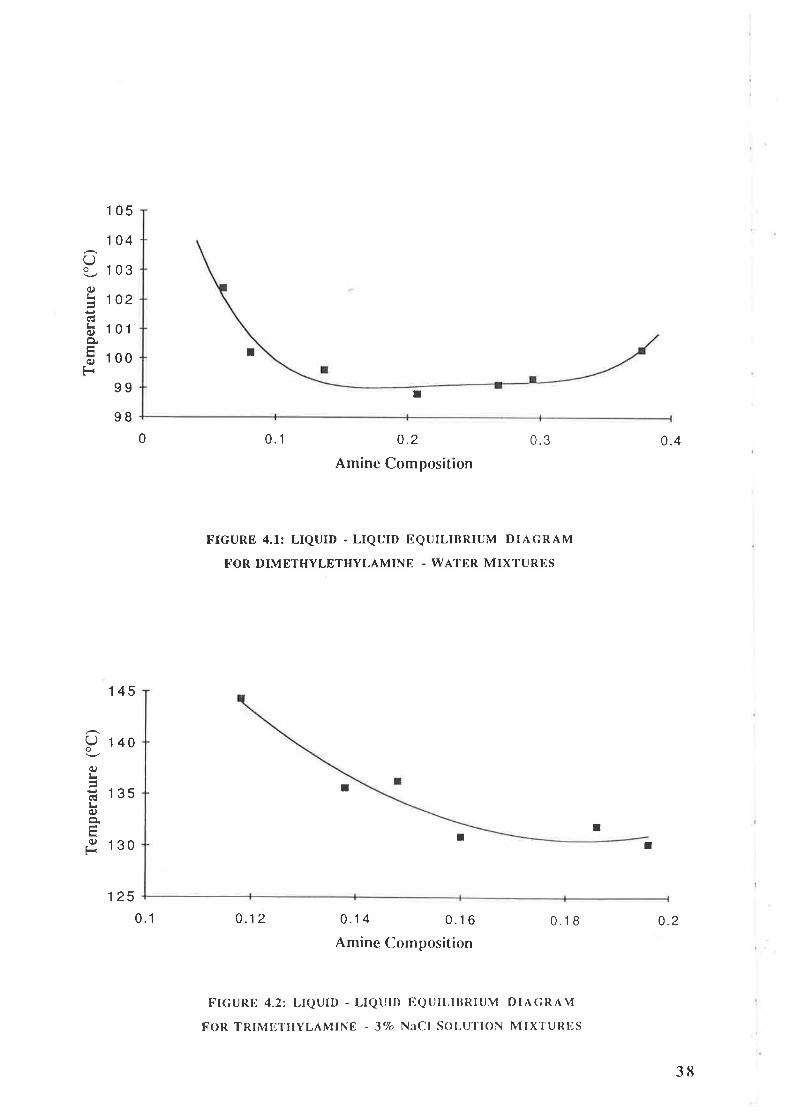
4.1 Licruid-Liquid Equilihrium Exneriments.
The liquid - liquid equilibrium phase diagram for mixtures of dimethylethylarnine and water is
summarised in figure 4.1. This figure is based on equilibrium data presented in Appendix A.
The shape of the equilibrium curve is typical of other aliphatic amine - water mixtures,
exhibiting lower critical solution temperature behaviour. Of particular interest is the high
temperature (approximately 3lZK) at which phase separation commences and the high
concentrations of both water in the amine phase and amine in the aqueous phase.
Phase separation was not observed for mixtures of trimethylamine and water at temperatures
below 433K. This represents the limit of the available equipment. However, phase separation
was induced by the addition of salt to mixtures of trimethylamine and water. This is not
surprising as Davison et. al. (1966) and Ting et. al. (1992) have also reported reductions in the
lower critical solution temperature for aliphatic amine - water mixtures with the addition of salt.
The liquid - liquid equilibrium phase diagram for mixtures of trimethylamine and 3Vo sodium
chloride solution is presented in figure 4.2. It is important to note that, for any given
temperature, the amine phase composition and aqueous phase composition read from figure 4.2
will not give the composition of two phases in equilibrium with each other. Each point on the
coexistence curve is determined separately with a fixed salt to water ratio. However, if a sffeam
containing trimethylamine, water and salt was separated into two liquid phases, the ratio of salt
to water would be different in each phase. Clearly, the addition of an extra component creates
an extra degree of freedom and a two dimensional equilibriurn curve can only be obtained by
adding a suitable constraint (e.g. fixing the ratio of salt to water).
It is eviclent from figure 4.2 that phase separation begins at even higher temperatures for
mixtures of trimethylamine in37o salt solution. Significant scatter in the experimental data is
indicative of the sensitivity of phase separation behaviour to snrall variations in the salt
concentration and to the presence of amine oxidation products (ref Section 3.1.1)
36

Errors between the measured salt concentration and that experienced in the ampoule at phase
separation conditions result from evaporation inside the ampoule upon heating, and flashing
during ampoule preparation.
Examination of the experimental data for other tertiary amine - water mixtures @avison et- al.,
1960), highlights a trend toward increasing lower critical solution temperatue and reduced
phase purity as the molecular weight of the tertiary amine decreases. The experimental data
presented for mixtures of dimethylethylamine and trimethylamine in water follows this trend-
37
105
T
103
1
c)o
q)
cl¡r(¡)
c)F
104
102
't
100
99
9B
0
I
IT
T
r135
Oo
(¡)¡i
ctt
qJ
(uF
145
140
130
125
0 0.'1 0.2 0.3
Amine Composition
FIGURE 4.1: LIQUTD . LIQUTD EQUILIBRIUM DTAGRAM
FOR DIMETHYLETHYLAMTNE . WATER MIXTURES
0 .12 0.1 8
0.4
0.20.14 0.16
Amine Composition
I.'ICURE 4.2: LIQUID - l,lQtJID I'IQUILItTRIUM DIr\GR^M
FOR TRIMfì'l'HYLAMINE - 3Vo NaCl SOI-UTION MIXl'URItS
0.1
3tì

4.1.1 Correlation of Liquid - Liquid Equilibrium Data'
For a consistent thermodynamic description of these mixtures, the liquid - liquid equilibrium
correration must arso correrate the vapour - riquid equilibriurn crata. If a separate correlation is
required to pred.ict vapour - riquid equilibria, a discontinuity will appear in the thermodynamic
descriPtion of the system'
unfortunately, atternpts to obtain a single model capable of accurate vapour - liquid and lquid -
Iiquid equilibrium prediction were unsuccessful' A more detailed thermodynamic model would
be required to simulate the complex temperature dependence of the liquid phase co-existence
curve
Consequently,amoreblackboxapproachwasusedinsimulationsofthenovelabsorption
cycle heat PUmPS
39

4.2 Vapour - Liquid Eauilibrium Experiments.
The vapour pressure of dirnethylethylamine - water mixtures was cletennined over the full range
of concentrations, at temperatures of 283.1 K,292.6 K,302.3 K,3IZ.0 K and 327.1 K. The
experimental data is presented in Appendix A.
The vapour pressure of trimethylamine - water mixtures was determined over the full range of
concentrations for temperatures of 283.8 K and 293.0 K. At higher temperatures, the vapour
pressure of some mixtures exceeded the range of the rnanometer. This restricted the
concentration range which could be examined at29l.5 K,302.1 K,312.4 K and 322.0 K.
The experimental vapour pressure data is summarized in Appendix A.
4.2.1 Correlation of Vapour Pressure Data.
At low pressures, the vapour phase composition can be calculated from the experimental data
by equating vapour and liquid phase fugacities for each cornponent. Under these conditions,
the fugacity coefficients nearly cancel each other and the Poynting corrections are close to unity.
This leads to the simplif,red expressions in equations 4.1 and 4.2.
Yttro P."u, : \Ítzo xft2o Puap,Hro
YA,r.r¡n" Pr'r"o* : YAntin. XAntin" Puup,A-in"
..(4. 1)
..(4.2)
Solution of these equations requires expressions for the liquicl phase activity coefficients (1,)
and the pure component vapour pressures (Puop,i). Ideally the model should also be capable of
preclicti¡g the l'reats of mixìng and hence the composition cleperrdence of stream enthalpy.
40
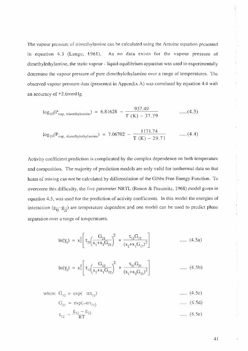
The vapour pressure of trirnethylamine can be calculated using the Antoine equation presented
in equation 4.3 (Lange, {961). As no data exists for the vapour pressure of
dimethylethylamine, the static vapour - liquid equilibrium appa-ratus was used to experimentally
determine the vapour pressure of pure dimethylethylamine over a range of temperatures. The
observed vapour pressure data (presented in Appendix A) was correlated by equation 4.4 with
an accuracy of t2.6mmHg.
logro(Pu^', rrimerhyramin") = 6.816 28 - 931 '49
r (K) - 37 .19
Ir71.7 4
(4 3)
(4.5a)
(4.sb)
(a.5c)
(4.5d)
(4.5e)
loglo(Puuo, dirnethylethyto,,.rin") = 7'06702T (K) - 29.1r
.(4.4)
Activity coefficient prediction is complicated by the complex dependence on both temperatue
and composition. The rnajority of prediction models are only valid for isothermal data so that
heats of mixing can not be calculated by differentiation of the Gibbs Free Energy Function. To
overcome this difficulty, the five parameter NRTL S.enon & Prausnitz,1968) model given in
equation 4.5, was used for the prediction of activity coefficients. In this model the energies of
interaction (Si¡-S;.,) are temperature dependent and one moclel can be used to predict phase
separation over a range of temperatures.
+lrrGn
(xr+x,G,2)2
where G,z = exp( -crt,")Gz, = exp(-ctt",¡
- 8rz - 8::'Ltz = RT
41

- Ezt - Ett'Lzt = RT
En- Ezz : ar* brT
Ezt-En = at+brT
(4.5Ð
(4.5e)
(4.5h)
The adjustable parameters al, a2,bp b, and ü, were obtained by minimising the error function
given in equation 4.6. The minimisation was solved, numerically, using a two stage Powell's
algorithm. For given values of b, and b' the error function was minimised by manipulation of
at, azand o. New values for b, and b, were chosen, and optimum values for a' q and o
recalculated. The process continued until no further reduction in the error could be achieved.
This two stage approach was chosen for its robustness. Attempts to minimise the error
function with a single stage Powell algorithm yielded varying results depending on the initial
values chosen for a,, a2,br b, and cr. The computer code for determining the adjustable
pa-rameters is presented in Appendix B.
Error: I meas Ygzo xuzo Puup.H2 o - YA-in. XA-in" Puap.Amin.
P..(4.6)
meas
Values for the five adjustable parameters are presented in table 4.1 for mixtures of
dimethylethylamine and trirnethylamine in water. Using these parameters, the experimental
vapour pressures could be predicted with an average accuracy of t4.9Vo and r5.97o for
dimethylethylamine - water and trimethylamine - water mixtures respectively. Adjustable
parameters were also obtained for diethylmethylamine/ water and cyclohexanelaniline mixtures
by fitting the 5 parameter NRTL model to literature experirnental data. Values for these
2parameters are also presented in
,t¡l
42

Cyclohexane - aliline
Diethylmethylamine - water
Dimethylethylamine - water
Trimeth larnine - water
al
t123.6
-3485.84620.0
3842.4
%
2453.8
-2584.t-2413.s
-4599.5
br
0.833
13.05
-r2.42-9.88
b2
-4.82ttr.209.90
16.5 8
ü,
0.4108
0.5021
0.6146
0.6107
TABLE 4.1: LBAST SQUARES FITTED NRTL PARAMETERS FOR TERTIARY AMINE - WATER
VAPOUR . LIQUID PHASE EQUILIBRIUM PRÐDTCTION
Figures 4.3,4.4 and 4.5 present comparisons between the calculated and experimental vapour
pressures of climethylethylarnine - water mixtures at283.1K, 302.3K and321.7K respectively.
The calculated dew point curues are also illustrated in these figures.
Examination of these figures suggests the presence of an azeotrope at a concentration of
approxrmately 987o dimethylethylamine. There is insufhcient experimenta-l evidence to confrm
or deny this observation. The bubble point curue also appears to flaten out at 32l.7Kand a. ?Ø',flu'"
composition of around 747o dimethylethylamine. This trend is consistent with the formation of - "
two liquid phases in ttris concentration range at higher temperatures.
Figures 4.6 and 4.7 present comparisons between the calculated and experimental vapour
pressures of trimethylalnine - water mixtures at 283.8K, 302.1K respectively. The calculated
clew point curves are also illustrated in these figures. The thermoclynarnic model is most
accurate at low amine concentrations due to the limited vapour pressure data available at
concentrations above 65 molo/o.
43

150
oo
q)
(â(âq)
È
I250
200
100
300
50
Bubble Point
0.20.8
FIGURE 4.3: VAPOUR - LIQUID PHASE ENVIìLOPE I.OR
DTMETHYLETHYLAMINE 'WATER MIXTURES AT 283'IK
Bubble Point Cu
01
0
0 0.1 0.2 0.3
0.4 0.6
Amine ComPosition
0.4 0.5 0.6
Amine Composition
0.7 0.8 0.9 I
00
600
0
5
400
300
200
100
à0
q)
rh(t){)
FIGURE 4-4: VAI'OUR - LIQUID PII^SFl Fl¡..vEt-OPE FOR
DTMETHYLE'THYLAMINE . WATER MIX'I'URIiS ^T
302'3K
Dew Point Curve
t
Dew Point Curve
I
I
Il
44

Dew Point Curve
1 000
1200
800
600
400
200
Bubb le Point Curve
o.2 0.8
FIGURE 4.5: VAPOUR - LIQUID PHASE ENVELOPE FOR
DIMETHYLBTHYLAMINE - WATER MIXTURES AT 321.7K
Bubble Point Curve
Iè0
q)¡rçt).â0)
È
0
1000
1200
800
600
400
200
0
0
0.4 0.6
Amine ComPosition
0.4 0.6
Amine Composition
èo
q)
ttØq)
È
0
0.2 0.8
FIGURTì 4.6: V^PoUR - LIQUID PHASE ENvELoPE l'-OR
.TRIMIì'THYLYAMINE . WATER MIXI'URIìS A'I 283.IìK
Dew Point Curve
I
45

2000
1600
1200
800
400
è0
q)L(t(t)0)LrÈ
Bubble Point Curve
0
0 0.1 0.2 0-3 0.4 0.5 0.0
Amine ComPosition
0.7 0.8 0.9 1
FIGURE 4.7: VAPOUR - LIQUID PHASE ENVELOPE FoR
TRIMETHYLYAMTNE - WATER MIXTURES AT 302'7K
Dew Point Curve
I
I
46

4.3 Calculation of Heats of Mixing.
As experimental heat of mixing data is not available for these mixtures, the heat of mixing was
calculated by differentiating the excess Gibbs Free Energy function (equation 4.7). The 5
parameter NRTL model Gibbs Free Energy function is obtained by manipulation of equations
4.5a and 4.5b to give equation 4.8.
H : -RT2 ..(4.7 )
(4.8)
e
Ge
RT : xrxz
where Tzr, Í2r, G, ancl G^ arc defined by equations 4.5c to 4.5h
This approach shouid provide reasonably accurate heat of mixing predictions over the
temperature range of the available experimental data (Skjold-Jorgensen et. al., 1980).
However, extrapolation into the region of liquid phase separation is not possible because the
Gibbs Free Energy function of equation 4.8 does not predict the true minimum energy in this
regron.,¡'l
.¿.
,,/, t;t((.,¡l l'tl /'
Calculated heat of mixing data, at 283 K,303 K and 323 K, are plotted in figures 4.8 and 4.9
for mixtures of dirnethylethylamine and trimethylarnine in water respectively. It is interesting to
note that the calculated heats of mixing appear to be quite sensitive to temperature. There is no
available experimental clata to verify this result. However, these calculations should be
reasonably accurate over this ternperature range because the temperature dependence of the
Gibbs Free Energy Function has been fitted to the experirnental phase equilibrium data.
47

oâD
F"
ao
X
è,o(Ëo
200 0
300 0
1 000
0
-1000
-2000
-4000
50"c
-30"C --'
0 .4 0.6
Amine Composition
10"c
3000
0 0.2 0.8
FIGURE 4.8: CALCULATED HEATS OF MTXING FOR
DIMETHYLETHYLAMTNE . WATER MIXTURES
-2000
è.0r-ào
x¿oCqq)
2000
1 000
0
-4000
-5000
1 000
30001 0"c
0 0.2 0.4 0.6
Amine Composition
0.8
FIGURE 4.9: CALCULATED HIìATS OIì MIXINC FOR
TRIMTì'THYLAMIND . WATT],R MTXTUR¡J'S
48

4.4 Calculation of Other Thermodvnamic Parameters.
The bulk of the necessary pure component physical properties of diethylmethylamine and
dimethylethylamine have not been measured. Hence, established group contribution estimation
techniques were employed to calculate these properties. The techniques used follow the
recommendations of Reid, Prausnitz and Poling (1987) and are summarised in table 4.2. For a
wide variety of compounds, the typical error between predicted and actual values using these
methods is less than2Vo. Data for other compounds was available in the PROCESS* Iibrary.
TABLE 4.2: THERMODYNAMIC PROPERTY ESTIMATION TECHNTQUES EMPLOYED IN THB
ANALYSIS OF THE NOVEL ABSORPTION REFRIGERATION CYCLB
PROPERTY ESTMAT'NTECI]MOUE
UNITS FORMULAE DEVELOPED FORDIMETTIYLETHYLAMINE
FORMULAE DEVELOPED FORDIETT{YLMETHYLAMINE
Ideal gasheat capacity
Joback(1984)
ltJmol 'K ' 23.23- t.t44xto-ZT + t6.45 - t.23xlo-2T +
2.54xr04 tz - t.oztxrO-7 t3 3.0lxl0+ 12 - t.zo3xt0-7 T3
+ 1.85x10⁻¹¹ I + 2.143x10-rr f
Liquid heatcapaclty
Chueh Jrnol-1K-l- Swanson
(1973)
171.8 202.2
Heat ofvaponsatron
Riedel(1954)
_lkJkg' 511- T 0.3 8 508-T
)0-3 8
3t7.6 1l - 309336.2
08 - 339
49

Chapter 5
THB NOVBL ABSORPTION REFRTGBRATION CYCLB
In this chapter, a novel absorption refrigeratíon cycle is proposed. A computer model of the
cycle is developed, based on the thermodynamic modeL described in chapter 4, and the results
of cycle performance simulations are presented. Based on these results, the potential of the
cycle is discussed.
A large body of literature, addressing various aspects of absorption cycle heat pumps has
developed since the pioneering work of Carre and Altenkirch (Stephan, 1983). A large fraction
of this resea¡ch effort has focussed on the discovery of new refrigeranf/ absorbent pairs.
However, the only working pairs to have found widespread commercial application are the
ammonia/ water and water/ lithium bromide pairs.
More desireable working fluid pairs may exist with improved properties such as toxicity,
transport properties or corrosivity. However, further investigation of new working pairs does
not appear to provide significant potential for further improvements in cycle thermodynamic
efficiency. O'Neill & Roach (1990) confirmed this observation by demonstrating that theAtt"
selection of/absorbenl refrigerant pair does not significantly alter the maximum theoretical (J^
performance achievable in an absorption refrigeration cycle employing an ideal distillation
column generator.
Consequently, further examination and synthesis of altenlative absorption refrigeration cycles
appears to offer the greatest potential for improving the perfonnance and cost of absorption
cycle heat pumps. An investigation into the losses encountered in conventional absorption
refrigeration cycles provides an ideal starting point in the sea¡ch for new cycles.
50

Recent papers by Briggs (1971) and Karakas et. al. (1990) have detailed an exergy balance on
the conventional absorption refrigeration cycle. These studies demonstrate that the majority of
losses are confined to the absorber and the generator. Dalichaouch (1990) calculated second
law efficiencies for an aqueous lithium bromide absorption refrigeration cycle. He showed
that, over a wide range of conditions, the performance of this cycle was less than thirty percent
of the performance predicted by the ideal second law.
Clearly, there is significant room for improvement in cycle performance. Two avenues exist
for improving the design of absorption refrigeration cycles . Firstly, improvements could be
achieved through modification of the conventional absorption cycle. Alternatively, performance
could be improved by creating a new type of absorption cycle. One example of the latter
approach replaces the conventional distillation column with a new separation process capable of
operating closer to the thermodynamic ideal.
References to the application of alternative separation techniques in absorption refrigeration are
sparse, suggesting that this is a potentially fruitful area for further investigation. With this in
mind, a novel absorption refigeration cycle was devised. The cycle was selected for further
investigation in this study.
The novel cycle, first proposed by Mehta (1981), employs a liquid - liquid separation step to
sepa.rate the absorbent from the refrigerant. The cycle has attracted scant attention in the
literature and analysis of the cycle appears to be restricted to the original patent. The cycle was
chosen for further examination with the intention of demonstrating the feasibility of eliminating
the distillation column generator in an absorption cycle heat pump.
The novel absorption cycle heat pump was simulated on a computer using the PROCESS*
chemical plant simulation software package. Results of the computer simulations are presented,
and the potential of the cycle is discussed.
5t
< I Refrioprqf inn l-wnlp flecnri nf r¡rn
Mehta (1981) describes a refrigeration cycle utilising the partial miscibility of some binary
mixtures, at elevated temperatures, to separate the refrigerant from the absorbent in an
absorptio n refrigeration cycle.
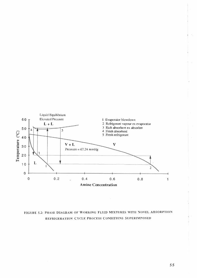
The cycle is illustrated in the flow schematic presented in figure 5.1. The physical significance
of each stream in the cycle is illustrated in the phase diagrams presented in figure 5.2.
Refrigerant vapour from the evaporator is dissolved in lean absorbent at low pressure. The rich
absorbent is pumped to high pressure and heated until the refrigerant becomes immiscible in the
absorbent. The refrigerant and absorbent are then separated in a settling drum. Recovered
refrigerant from the settling drum is cooled and passed to the evaporator. The lean absorbent is
returned to the absorber. The novelty of this cycle lies in the method for separation of the
refrigerant from the absorbent. This is carried out in the liquid phase.
There are significant differences between the cycle illustrated in figure 5.1 and the original cycle
proposed by Mehta (1981). These differences are listed below;
(Ð The liquid blowdown (containing the bulk of the less volatile component) is continuously
removed from the evaporator, pumped to high pressure and returned to the settling drum.
In contrast, the evaporator blowdown was passed to the absorber in the cycle proposed by
Mehta. Analysis shows that this modification provides a significant improvement in
thermodynamic efficiency. Unfortunately, the liquid - phase separation is imperfect.
Hence, the absorbent stream retains a fraction of the more volatile component and some of
the less volatile component remains in the refrigerant. Consequently, the evaporator
blowdown stream is large. By returning the evaporator blowdown directly to the
generator, the load on the absorber is recluced and thermodynamic performance is
increased.
52
(iÐ A heat exchange network for recovering heat from the hot refrigerant and absorbent
streams is defined. These heat exchangers preheat the feed to the settling drum.
The principal differences between the novel absorption refrigeration cycle and the conventional
absorption refrigeration cycle (illustrated in figure 2.I) are as follows:
(Ð The liquid - liquid separation drum replaces tlìe distillation column in the conventional
cycle.
(iÐ Liquid blowdown from the evaporator is recyclecl to the separation drum generator.
(iü) The novel absorption retrigeration cycle does not require a condenser
Preliminary examination of the cycle highlights the potential for reductions in capital cost, over
the conventional cycle, througl.r the elirnination of the condenser. There is also potential for
increasing thermodynamic performance as heat is not required to vaporise the refrigerant.
Ideally, the bulk of the heat required to raise the temperature of the rich absorbent and the
evaporator blowclown can be recovered by cooling the fresh absorbent and fresh refrigerant.
53

Pump
Absorber
Refrig Return Pump
Heat Input
Coo
vaporator
Refrigeration
LiquidSeparationVessel
FIGURE 5.1: FLOW SCHEM^I.IC OF THE NOVBL AIISORPTION REFRIGERATION CYCLE
54
60Liquid EquilibriumElevated Pressure
L+LI Evaporator blowdown2 Refrigerant vapour ex evaporator3 Rich absorbent ex absorber4 Fresh absorbent5 Fresh refrigerant
()o
q)¡r
GI¡r(uq
q)t-(
5450
40
30
20
V
L
0.2 0.4 0.6
Amine Concentration
0.8
FIGURE 5.2: PHASE DIAGRAM OI.'WORKING FLUID MIXTURES WITH NOVEI, ABSORPTION
REF'R.IGERATION CYCLE PROCESS CONDITIONS SUPERIMPOSET)
20
0
1
10
3
Pressure = 67.24 mmHg
V+L
55

< ) Splonfinn nf Wnrl¿in<¡ ['lrri¡lc fnr fho Nnval Cvnla
A suitable refrigerant/ absorbent pair for this cycle must exhibit "lower critical solution
temperature behaviour" when mixed. The selected pair should also possess propefiies which
are desirable in conventionai absorption refrigeration working fluids. These properties are
discussed in chapter 2.
Relatively few mixtures exhibit lower critical solution temperature behaviour. The bulk of such
mixtures are composed of amines with either water or ethanol. In these systems, miscibility at
low temperatures is a consequence of hydrogen bonding between the amine group and the polar
solvent. At higher temperatures the hydrogen bonds breakdown, reducing the affinity between
the amine and the solvent.
Figure 5.3 summarizes the tiquid-liquid equilibrium co-existence curves for mixtures of
dimethylethylamine, diethylmethylamine and triethylamine with water. It demonstrates that the
lcwer boiling point amines have a higher "lovr'er critical solution temperature" and reduced
purity in the equilibrium phases. Examination of other amine - water phase cliagrams (Davison
et. al., 1960) indicate that such behaviour is typical of amine - water mixtures.
Consequently, if a low boiling point amine is used as a refrigerant in this cycle (with water as
the absorbent), the thermodynamic perfonrance of the cycle will be lowered by imperfect
separation in the settling clrum. Subsequent distillation of these phases may be required to
improve performance.
Conversely, if a high boiling point amine is selected in the cycle as the absorbent (with water as
the refrigerant), then the refrigerant ancl absorbent will be immiscible at all reasonable
refrigeration temperatures. For this reason, it would not be practical to clesign the cycle under
these conclitions.
56

100
120
BO
60
40
20
Dimethylethylamine - water
lmethylamine - water
0.4 0.6
Amine Composition
Triethylamine - water
0.8
Oo
(9
cÉtrq)q
q,)
F
0
0 0.2 1
FIGURE 5.3: LIQUID . LIQUID PHASE EQUIT-II}RIA FOR VARIOUS
TERTI^RY AMINE/ WATER MIXTURES
57
< î l-nrnnrrfar Sirn¡rlofinn nf f hp Nnwpl Cvnle
Computer models were constructed for the novel absorption cycle heat pumps to determine the
process conditions through out the cycle and the cycle thermodynamic performance. The
results of these simulations provide evidence of the feasibility of the proposed cycle.
5.3.1 Thermodynamics
Detailed thermodynamic models for the prediction of phase equilibria and state properties such
as enthalpy and entropy are required to obtain accurate simulation results. Equilibrium
predictions and excess properties were calculated using a five parameter NRTL model
(Asselineau and Renon, l91O) fitted to the experimental data. Pure component heat capacities
and latent heats were calculated using established group contribution methods (Chueh and
Swanson, I973, Joback, 1984 and Riedel, 1954). The five parameter NRTL model and the
appropriate group contribution methods a¡e described in more detail in chapter 4.
In subsequent computer simulations of the novel absorption cycle heat pumps, the
thermodynamic models were extrapolated to temperatures above the range of the experimentally
determined data. Unfortunately, higher temperature experimental data could not be obtained
because of the limiæd measurement range of the mercury manometer.
Attempts to obtain a single model capable of accurate vapour - liquid and lquid\- liquid ...:/
equilibrium prediction were unsuccessful. In cornputer simulations of cycle performance,
either a second thermodynamic model or a black box component splitter was used to simulate
the liquid - liquid separation step. Both techniques irnply a discontinuity in the thermodynamics
of the cycle.
58

ru5.3.2 The PROCESS Simulation Package
The PROCESS* chemical plant simulation software package was used in all computer
simulations of the absorption cycle heat pumps. This package is used extensively in the design
and operation of commercial hydrocarbon processing and petrochemical plants. It can solve
complex material and energy balances and, with an appropriate thennodynamic model, it can
predict phase equilibria. This makes the prograrn particularly useful for the design of complex
physical separation processes which include recycle streams and distillation columns.
PROCESS assumes perfect mixing in all phase separation calculations.
Sample PROCESS input and output hles, used in simulations of the novel absorption cycles,
are presented in Appendix D. The solution procedure employed by the PROCESS simulation
program in these cases is also presented.
Unless otherwise specified in the input file, PROCESS calculates new values for the process
conditions of the recycle stream by direct substitution. It is interesting to note that the results
obtained from these simulations were often sensitive to the allowable error (tolerance) between
the old and new recycle stream temperature. Care was taken to ensure that the specified
tolerances were suff,rciently tight to prevent this from significantly influencing the results.
5.3.3 Simulation Constraints
There are a number of variables which influgnce the cost and performance of abso¡ption cycle
heat pumps. The performance of an ideal, reversible absorption cycle is defined solely by the
temperatures at which heat is addecl and rejected from the cycle. However, the performance of
any real cycle is also dependent on a number of variables specific to the cycle. These variables
are discussed below. From this list, a consistent set of design constraints was selected to
enable comparison of the va¡ious cycles.
59

(i) Generator. condenser and absorber temperatures.
These temperatures are largely set by the temperatures of the available heat source and heat
sink. However, some allowance must also be made for a reasonable temperature difference
between the fluid on the utility side and the fluid on the heat pump side of each heat exchanger.
When simulating the performance of the novel absorption refrigeration cycles, the generator and
absorber temperatures were fixed with the assumption that the hot and cold utilities were
available at appropriate temperatures. This was required because the boiling point elevation
between the evaporator and the absorber was not sufficient to achieve realistic absorber
temperatures.
(ii) Evaporator temoerature.
While other parameters are generally set within a reasonably narrow band for all absorption
refrigeration applications, the evaporator temperature can vary dramatically depending on the
required refrigeration task. For this reason, the influence of evaporator temperature on the
objective parameter was investigated in some detail.
(iii) Approach temperature in the heat recovery heat exchangers.
Reducing the approach temperature in the heat recovery heat exchangers increases cycle COP
but also increases capital costs. In conventional cycles, one would expect approach
temperatures of a¡ound 10 to 20K. However, significantly lower approach temperatures ,were
required for the novel absorption cycles because of the low boiling point elevation achievable
with the selected mixtures. An approach temperature of 2 K was selected for the basic novel
absorption heat pump cycles and 5 K for the novel cycles with distillation.
60

(iv) Rich absorbent quality.
Rich absorbent exiting the absorber must be a liquid to ensure that it can be pumped up to the
pressure of the generator. However, sub-cooling of the rich absorbent results in an
undesir/able increase in absorbent circulation rate. The lean absorbent flowrate was set to "/ensure that liquid at its bubble point exits the absorber in all simulations. This would be
difhcult to achieve in practice but sets an upper limit on cycle perfonnance.
liv) Evaporator blowdown.
The fraction of fresh refrigerant boiled in the evaporator has a dramatic influence on the
performance of the novel absorption cycle heat pumps. If the fraction of refrigerant boiled in
the evaporator is increased, the evaporator (and hence absorber) pressure goes down and the
flowrate of required absorbent increases. This is balanced to some extent by the increase in
refrigeration achieved. An optimum exists for a given absorber temperature, evaporator
temperatue and working fluid purity.
An example of this is presented in figure 5.4 for the basic novel absorption refrigeration cycle
with methyldiethylamine and water as the working fluids. For a 1OoC evaporator temperature
and 20oC absorber temperature, the optimum COP was obtained when around 70Vo of the
incoming refrigerant was returned to the generator.
V/hile the influence of evaporator blowdown is more dramatic for the novel absorption cycles,
an optimum blowdown rate also exists for tlle conventional cycle. The evaporator blowdown
was optimised to achieve the maximum coefficient of performance in simulations of each
absorpti on refri geration cyc le in vesti gated.
61

q)Iñfr€¡rc)
O.
q)
It=q)
O
0.48
0.46
0.44
0.42
0.5
0.4
0.3 B
0.4 0.5 0.6 0 .7 0.8
Fraction of Liquid Exiting Evaporator0.9
FIGURE 5.4: OPTTMUM BLOWDOWN EX^MPI,I.] F-OR .I'}II.] NOVEL
ABSORPTION REFRIGERATION CYCI,¡ì
62

{ 4 Nnvpl Ähcnrnf inn Rpfrioprcfinn Cvclp Sirnrrl¡finn Resrrlfs
The performance of the novel absorption refrigeration cycle was investigated using the general
constraints detailed above. Initial simulations employed diethylmethylamine and water as
working fluids in the cycle. This provided an ideal starting point as experimental phase
equilibrium data was available in the literature and comparisons could be made with the analysis
presenred by Mehta (1981).
A generator temperature of 80oC was used for all simulations with diethylmethylamine and
water. At this temperature the slope of the co-existence curve is very steep and only small
improvements in phase purity are possible.
A process flow diagram of the novel absorption refrigeration cycle, with the evaporator
temperature and absorber temperature fixed at 10oC and 20oC respectively, is presented in
Figure 5.5. The diagram includes details of the process conditions for each stream in the cycle.
Examination of the stream data highlights the following points.
(Ð The refrigerant exiting the generator is not very pure in the more volatile amine. This
necessitates a large recycle stream for the spent refrigerant exiting the evaporator.
(iÐ The evaporator must operate under vacuurrì to achieve even modest refrigerant
temperatures in the evaporator.
(iii) The ratio of absorbent to refrigerant flowrates is very high compared to conventional
cycles, despite the small temperature difference between the evaporator and the absorber.
Poor cycle performance would be expected as a consequence of the high absorbent
circulation rate.
Figure 5.6 illustrates the effect of evaporator temperature on the optimum coefficient of
performance with the absorber temperature fixed at 20oC. Thermodynamic performance is
reduced as the evaporator temperature is decreasecl and the cycle ceases operation at evaporator
temperatures below about 2oC.
63

5
Absorber
Input
Refrig Pump
Coo
Evaporator
Refrigeration
LiquidSeparationVessel
A Pump
9
Generator Duty: 1.28MW Evaporator Duty:0.62MV/ Absorber Duty = 1.92MW
Absorbent Heat Recovery Duty =7.l2MW Refrigerant Heat Recovery Duty = 1.04MW
Absorbent Return Pump = 0.02MW Refrigerant Return Pump = 0.002MV/
STREAMNO r234s6189
Flowrate (kmol h-1)
Composition (mole7o)
Temperature ("C)
Pressure (kPa)
Liquid Fraction
326
65.0
80.0
333
1.0
326
6s.0
32.3
333
1.0
215
52.8
r0.1
333
1.0
215
52.8
78.0
333
1.0
lll88.7
10.0
8.96
0.0
6014
l.l80.0
333
1.0
6014
l.t22.1
333
1.0
6125
2.7
20.1
333
1.0
6125
2.1
't r.9
-)-1 J
1.0
I.-IGURE 5.5: PROCIìSS FLOW DI^GfìAùl OI.'THE NOVEL
AIISORPTION REI'RtGIìRA'TtON CYCLE
64

0.2
0
o)(J
cl'
¡r
¡re)
Þ<
o
(u(J
(¡,)
ôL)
0.6
0.5
0.4
0.3
0
0 2 468Evaporator Temperature (oC)
10 '12 14
FTGURE 5.6: THE INFLUENCE OF EVAPORATOR TEMPERÂTURE ON TfiE PERFORMANCE
OF THE NOVEL ABSORPTION REFRICERATION CYCLE
(DIETHYLMETHYLAMINE AND WATER WORKING FLUIDS)
65

This behaviour ca¡r be explaineci by inspection of the pha.se cliagram presented irr figure 5.2. As
the evaporator temperature decreases, tlie evaporator (and hence absorber) pressure decreases.
The absorbent ci¡culation rate must then be increased to lower the concentration of amine in the
rich absorbent, and maintain the desired temperature in tlie absorber. Increased losses and
reduced performance result from the increased circulation rate.
Further reduction in the rich absorbent amine concentration is not possible when the equilibrium
composition exiting the absorber equals that of the lean absorbent entering the absorber. The
minimum possible evaporator temperature is achieved under these conditions.
In another set of simulations with the diethylmethylamine - water pair, the coefficient of
performance of the cycle was determined over a range of absorber temperatures with the
evaporator temperature f,rxed at l0oc. The coefficient of perfonnance decreased with increasing
absorber temperature (hgure 5.7).
0.6
0.5
0.4
3
0.2
0.1
16 18 20 22 24Absorber Temperature (.C)
26 28
I.-ICURIi 5.7: THE INFLUENCI.ì OF ABSORßER TEMt'FlR^l'URIì ON THE, PERf.'ORM^NCE
OF' THE NOVIìL AIISORPI-ION REFRIGIìRATION CYCLE
(DIETHYLMTiTHyt-^MrNE /rND WI\TER WORKING FLUTDS)
\/l
0
(uac!
lr-oLr(¡)0(
q)
I
(uoO
0
66

The boiling point elevation achieved in the novel absorption refrigeration cycle with
diethylmethylamine and water is clearly inadequate for practical refrigeration. New working
fluids were sought in an attempt to improve the performance of the cycle and raise the allowable
absorber temperature. Working fluids with increased normal boiling point difference were
particularly sought after with the expectation that increased boiling point elevations could be
achieved between the evaporator and the absorber.
Dimethylethylamine - water and trimethylamine - water mixtures were selected as candidate
working fluids with potential in the novel cycle. 'While dimethylethylamine and trimethylamine
have low boiling points, liquid phase immiscibility had not previously been observed for these
mixtures. The necessary experimental data was gathered to allow simulation of the novel
absorption cycle with dimethylethylamine - water mixtures. The experimental difficulties of
obtaining high pressure vapour - liquid equilibrium data for a three component mixture dictated
that a more limited experimental investigation and cycle analysis be conducted with mixtures of
trimethylamine, water and salt. This analysis is described in chapter 6.
A fixed generator temperature of 100oC was used in simulations of the novel absorption
refrigeration cycle with dimethylethylamine and water. Figure 5.8 illustrates the influence of
evaporator temperature on performance for this cycle. The boiling point elevation achieved was
very similar to that obtained in the diethylmethylamine - water cycle. However, the coefficient
of performance was considerably lower. This reduction in perforrnance is attributed to the high
specific heat of the refrigerant, caused by water (absorbent) contamination. Synthesis of an
improved heat recovery design could reduce the apparent difference in cycle performance when
using alternative working fluids.
67

q)Icll
q)Ào
oa
c)ôc)
0.05
0.04
0.03
o.02
0.01
0
7 B 9 10 11
Evaporator Temperature ('C)'12 13
FICURE 5.8: l'HE INFLUENCE OF EVAPORATOR TEMPER^TURE ON THE PERFORMANCE
OF THE NOVEL AI}SORPTION REFRTGERATION CYCLE
(DIMETHYLETÍTYLAMtNE AND WATER WORKTNG FLUTDS)
68
5.5.1 Thermodynamic Analysis
To confirm the results of_these simulations and explain why the cycle is a valid method for,,,, \
obtaining refrigerationi*9)-urt investigate the phase behaviour of these mixtures in more )
detail.
5.5 Discussion
It is clea¡ from these simulations, that the novel absorption refrigeration cycle is inferior to the
conventional cycle. Cycle operation is only possible over a limited range of temperatures, and
the coefficient of performance is poor compared with conventional absorption refrigeration
units using ammonia and water as the refrigerant/ absorbent pair.
However, these calculations are significant as a tool to verify the feasibility of the proposed
cycle. If the cycle is feasible, then vaporisation of the refrigerant is not a requirement for
refrigerant recovery and other candidate unit operations should be investigated in more detail.
A typical lower critical solution temperature phase equilibrium curve is presented in Figure 5.9.
Superimposed upon the liquid phase co-existence curve are two constant pressure bubble point
curves. At low pressures, the bubble point temperature increases as the concentration of the
more volatile cornponent is increased. At higher pressures the bubble point curve intersects the
region of liquid phase immiscibility. Over this concentration range, the bubble point
temperature remains constant. Either sicle of the immiscible region, the bubble point
temperature increases as the concentration of the more volatile component is increased.
69

140
120
100
BO
60
40
20
0
vC-)o
q,)
dq)
q)F
V+Lmm Hg
LLiquid EquilibriumL+L
v
LV+Lhessure = 67.24 mmHg
0.2 0.4 0.6
Amine Concentration
0.8
F'IGURE 5.9: PHASE EQUILIBRIUM DI^GR^MS FOR'f YPICAI- MIX'IURES EXHIBITING
LOWER CRITICAL SOLUTION TEMPERATURE BEHAVTOUR
The behaviour of the bubble point curves, ciescribed above, can be cleduced by inspection of
equation 5.1 (Bett et. al., 1975).
0
(s.l)
where Ax, is (yz- xz),Ah¡ is the difference between the pârtial enthalpies of contponent i in
rhe vapour and liquid phases 0rf - nl). S.- is tlre seconcl cìerivative ot tlte partial Cibbs Free
Energy function at constant pressure and ternperature. and (dT / dxr)p is the derivative along
I
the saturatior.t curve-
10

The second derivative of the partial Gibbs Free Energy function, and hence the derivative of the
bubble point temperature, ate zeto at the lower critical solution temperature. Elsewhere the
second derivative of the partial Gibbs Free Energy function must be positive to ensure phase
stability (equation 5,2).
l.e
The tertiary amine - water mixtures, ernployed in simulations of the novel absorption
refrigeration cycle, do not exhibit azeotropic behaviour nea¡ the immiscible region. This can be
deduced from the calculated vapour phase compositions which are rich in the more volatile
amine. Given these constraints, Âx, must be negative and (dT / dxz)p must be positive in the
region below the liquid - Iiquid phase equilibriurn curve.
Now, if we take a mixture in the immiscible region where (dT / dx2)p is zero, it will separate
into two liquid phases of equal boiling point. If we drop the pressure of the two streams to a
region of total miscibility (where (dT / dx2)p is positive) then a difference must occur between
the boiling points of the two streams. This difference in boiling points can be used to create the
the necessary boiling point elevation between the evaporator and the absorber, and conhrms the
feasibility of the proposed novel absorption refrigeration cycle.
[4r.,],' o ..(5.2)
1l

5.5.2 Comparison with Literature Results
The novel refrigeration cycle has attracted little attention in the literature. The limited analysis of
cycle performance by Mehta (1981), in the original patent, appears to be the sole reference for
comparison of the results obtained in this study.
Differences between the assumptions used in the performance calculations presented by Mehta
(1981) and those employed in this study are given below.
(i) Assumed stream compositions
The compositions of the refrigerant and absorbent steams, employed by Mehta, were 88.0wt7o
and 3.0wf7o amine respectively. In this study, the assumed compositions of the refrigerant and
absorbent streams were 90wt7o and 5.lwtVo respectively. These values were obtained from
experimental data presented in graphical form by Hood and Davison (1960).
(ii) Evaporator blowdown return
In this study, performance \ /as improved by recycling the evaporator blowdown directly to the
generator. This is explained in more detail in section 5.1.
(iii) Heat recovery heat exchaneer network
Performance calculations presented by Mehta assume a 4 K difference between the temperature
of the streams entering and exiting the liquid phase separator. A 4 K temperature difference
between the lean absorbent entering the absorber and the rich absorbent exiting the absorber
was also assumed. The heat exchanger network used to achieve this level of heat recovery was
not described. In this study, a realistic heat exchanger network was employed.
12
For an absorber terxperature of 29"C and evaporator temperature of 10oC Mehta obtained a COp
of 0.84. This performance is signihcantly better than that obtained in this study, even though a
superior cycle was employed.
The difference in performance can be traced to the ideal heat exchanger network employed in
the analysis presented by Mehta. The exergy analysis presented in section 5.5.3 demonstrates
that the majority of losses in this cycle occur in the heat recovery exchangers. For this reason,
improving the heat exchange network would be expected to make significant improvements to
the performance of the cycle. Alternatively, the cycle could be improved by blending a portion
of the rich absorbent with the returning evaporator blowdown to better match the required
cooling duties in the two heat recovery exchangers. Even so, a constant thermal driving force
across these heat exchangers is unlikely to be achieved because of the large changes occuring in
the stream partial excess enthalpies at constant composition.
73

5.5.3 Exergy Analysis
In an attempt to identify the reasons for the poor performance of this cycle, an exergy analysis
was conducted on the novel cycle. For ease of calculation, the total exergy loss from each unit
in the cycle was calculated using the simplified equations proposed by Linhoff & Carpenter
(1981). The accuracy of the available data did not warrant more detailed availability
calculations. The calculated exergy losses (summarized in table 5.1) are based on a
refrigeration duty of 478kW and consumption of LP steam at 100"C.
UNrr EXERGY LoSS PcnCBNTAGE OFTOTAL(7o)
Generator
Absorbent heat recovery
Refrigerant heat recovery
Absorber
Valve
Evaporator
35.3
61.9
28.1
50.7
3.3
6.0
19.1
33.4
t5.221.4
1.8
3.2
TABLE 5.1: SOURCE OF EXERGY LOSSES IN THE NOVEL CYCLE
The percentage of losses oecurring in the generator of the novel cycle is considerably lower
than that reported by Briggs (1971) for conventional absorption cycle generators
(approximately 39.07o). Clearly, the new design was successful in reducing relative losses in
the generator, but the increased circulation rate of absorbent and refrigerant required in this
design resulted in large losses in the two heat - recovery heat exchangers.
These results suggest that it rnay be possible to increase the perfonnance of the novel cycle by
employing a distillation step to improve refrigerant or absorbent purity. This would effectively
reduce losses in the heat exchangers but additional losses would be incuned in the distillation
colurnn. The potential of these cycles is discussed further in chapter 6.
74

Chapter 6.
VARIATIONS OF THE NOVBL ABSORPTION
REFRIGERATION CYCLE
In this chapter, a number of variations of the basic novel absorption refrigeration cycle are
proposed. These cycles include an additional distillation step to improve refrigerant andl or
absorbent puríty. Results of computer simulations are presented and the potential of these
cycles is discussed. The potential of trimethylamine - 37o aqueous salt solution is also
analysed.
In chapter 5, inferior thermodynamic performance was obtained in simulations of the basic
novel absorption refrigeration cycle employing the available absorbent/ refrigerant pairs.
Unfortunately, there are very few alternative absorbent/ refrigerant pairs, exhibiting suitable
phase behaviour, which can be considered to overcome the limitations of this cycle.
However, further improvements in cycle performance could be obtained by modifying the basic
cycle. A number of variations to the basic cycle can be devised by including additional
distillation steps in the cycle. These modifications improve the purity of the absorbent and,/ or
refrigerant with a consequent reduction in the absorbent circulation rate. Unfortunately, the
addition of the distillation step also adds complexity to the basic novel abso¡ption refrigeration
cycle. A general discussion of these modifications is presented in this chapter together with the
results of computer simulations of each cycleis thermodynamic perfonnance.
In chapter 5, discussion of the basic novel absorption refrigeration cycle, with trimethylamine
and water, was deferred because of the difficulty in conclucting a full analysis with the limited
available experimental data. A simplihed analysis of the application of these mixtures in the
novel absorption refrigeration cycles is presented in this chapter.
75

6.1 Description of Novel Ahsorption Refrigeration C.vcles Which Include
An Additional Distillation Step
A number of cycles which include an additional distillation step can be devised. The primary
goal of the additional distillation step is to increase the purity of the absorbent and/ or the
refrigerant streams so that increased boiling point elevations can be achieved between the
evaporator and the absorber. Increasing absorbent purity also reduces absorbent circulation
rates, with a consequent improvement in cycle perforrnance.
If the boiling point elevation between the absorber and the evaporator is increased beyond that
obtained in the basic novel absorption refrigeration cycle, the concentration of amine in either
the evaporator blowdown or the rich absorbent sffeam will be outside the concentration range of
the immiscible region. Consequently, it will not be possible to purify this stream in the liquid
phase separation drum. Purification would, instead, be achieved by feeding the stream directly
to the distillation column. Cycles can be devised which employ the liquid phase separation step
for partially purifying either the evaporator blowdown or the rich absorbent.
Low molecular weight tertiary amine - water mixtures can sep¿ìrate into two liquid phases at
elevated temperatures. However, the aqueous phase generally contains a significant quzurtity of
amine and the amine phase contains large quantities of water. The poor separation obtained in
this liquid separation step makes additional distillation steps particularly attractive when utilising
these mixtures as working fluids. One or both of the streams exiting the liquid phase separation
drum can be distilled.
76

6.1.1 Absorbent Phase Distillation
Figure 6.1 illustrates a cycle which combines distillation and liquid phase separation steps to
recover refrigerant from the rich absorbent stream returning from the absorber. The rich
absorbent first enters the liquid phase separation drum where a portion of the refrigerant is
recovered. The partially regenerated absorbent is then passed to the top tray of the distillation
column and a more pure absorbent is removed from the bottom of the column. The column
overheads a¡e combined with the refrigerant rich phase exiting the liquid phase separation drum
to produce the fresh refrigerant feed to the evaporator. In this cycle, the evaporator blowdown
is passed to the absorber in a simila¡ manner to the conventional absorption refrigeration cycle.
Unfortunately, for all known working fluid pairs, the fresh refrigerant entering the evaporator
contains a significant quantity of the absorbent. Consequently, the flowrate of the evaporator
blowdown is high and the absorbent flowrate must be increased to prevent evaporation of the
evaporator blowdown in the absorber.
Losses, resulting from the high absorbent circulation rates, can be reduced by returning the
evaporator blowdown to the regeneration section of the cycle. However, the available feed
locations for the returning evaporator blowdown are unattractive.
The liquid phase separation drum is not an ideal feed location because the concentration of
amine in the evaporator blowdown is too high for effective liquid phase separation.
A better cycle is illustrated in figure 6.2. In this cycle, the evaporator blowdown is used as
reflux to the distillation column. The partially regenerated absorbent is fed into the column
below the top tray. The resulting rectification section of the column produces a significantly
higher purity refrigerant. Simulation results for this cycle are presented in section 6.3.1.
77

Bvap oratorConde
id
Vessel
FIGURE 6.1: FLOW SCHBMATIC OF A NovEL ABSORPTION REFRIGERATION CYCLE
WITH ABSORBENT PHASE DISTTLLATION AND EVAPORATOR BLOWDOWN TO THB ABSORBER
refrigerantphase
Heat
Rich AbsorbentReturn Pump
Absorber
Refrigeration
istillation
trippingection Only
Reboiler
78

CondenserRefrigerantPhase
FIGURE 6.2: FLOW SCHEMATIC OF A NOVEL AßSORPTION REFRIGERATION CYCLE WITH
ABSORBENT PHASE DISTILLATION AND EVAPORATOR ßLOWDOWN RETURNED TO THE
DISTTLLATTON CO LUJ\,IN.
Rich AbsorbentReturn Pump
Evaporator
Absorber
Refrig ReturnPump
Blowdown
RectifyingSection
Heat
Absorbent
Reboiler
on
Liquid
Vessel
DistillationColumn
StrippingSection
79

The low concentration of refrigerant in the refrigerant rich phase exiting the separation drum
compared with that exiting the distillation column suggests the possibility of feeding both
streams from the separation drum onto separate trays in the column. However, the optimum
feed location for the two streams would be identical because of the small difference in the
boiling point of the two streams. Clearly, this creates a cycle iclentical to that of the
conventional cycle.
6.1.2 Refrigerant Phase Rectification
Figure 6.3 illustrates an alternative cycle in which the refrigerant rich phase exiting the liquid
separation drum is distilled to increase the purity of the refrigerant. First, the rich absorbent
enters the liquid phase separation drum where the refrigerant is separated from the absorbent.
The refrigerant rich stream is then passed to a distillation column containing both rectification
and stripping sections. Pure refrigerant is removed from the top of the column and lean
absorbeni, removed from the bottom of the column, is combined with tlie absorbent stream
exiting the liquid separation drum.
Unfortunately, all fresh refrigerant produced in this cycle is obtained by vapourisation in a
distillation column. This partially defeats the purpose of the original cycle which eliminates the
necessity for a phase change in the regeneration step. However, the advantage of this cycle lies
in the small fraction of the refrigerant rich absorbent stream which must be processed in the
distillation column. Simulation results for this cycle are presented in section 6.3.2
As the refrigerant can be distilled to achieve high purity, the evaporator blowdown stream will
be small. This allows the blowdown to be passed to the absorber without excessive penalty.
However, one would still expect superior performance if the evaporator blowdown were
returned to the clistillation column as reflux. Analysis of the benefits of returning the evaporator
blowdown as reflux to the distillation column in a conventional cycle will be discussed in detail
in Chapter 8.
80

Condenser
RefIuxDrum
RectificationSection
LiquidSeVessel
aporator
Rich AbsorbentReturn Pump
StrippingSection
Reboiler
DistillationColumn
FIGURE 6.3: FLOW SCHEMATIC OF A NOVEL ABSORPTION REFRIGERATION CYCLE
WITH REFRIGERANT PHÂSE RECTÍFICATION
8l

6.1.3 Liquid Phase Refrigerant Recovery from the Evaporator Blowdown
Figure 6.4 illustrates an alternative novel absorption refrigeration cycle in which refrigerant in
the evaporator blowdown is partially recovered in a liquid phase separation d¡um. The
blowdown stream exiting the evaporator is heated in a heat recovery exchanger. It is then
passed to the liquid phase separation drum where additional heat is supplied and phase
separation occurs. The refrigerant rich phase is combined with the fresh refrigerant and
returned to the evaporator. The absorbent rich phase exiting the liquid separation drum is
passed to the absorber.
In this cycle, the composition of the liquid blowdown from the evaporator is such that liquid
phase separation will occur upon heating. However, to achieve significant boiling point
elevation between the evaporator and the absorber, the refrigerant concentration in the rich
absorbent must be below that required for liquid phase separation. Consequently, separation of
refrigerant from the rich absorbent is achieved in a single distillation column containing both
rectifying and stripping sections.
The attraction of this cycle lies in the ability of the cycle to obtain useful refrigeration from a
greater fraction of the fresh refrigerant from the distillation column. Unfortunately, the cycle
requires a reasonably elaborate heat recovery network. Simulation results for this cycle are
presented in section 6.3.3
82

S
Liquid
Vessel
Drumvaporator
Absorber
Reboiler
geration
Columnation
EvaporatorBlowdown
Return PumpRich
Heat RecoveryExchangers \
Heat
Condenser
FIGURE 6.4: FLOW SCHBMATTC OF A NOVEL ABSORPTION REFRIGERATION CYCLE \ryITH
LIQUID PHASB EVAPORATOR BLOWDOWN REFRIGBRANT RECOVERy
83

6.2 comnuter Simulat.ion of cucles Incluclins Distillation
The PRoCgSSTM chemical plant simulation package was used to model the performance of
each cycle variation. The main differences between the solution procedure employed for these
cycles and that employed for the basic novel absorption refrigeration cycle, discussed in chapter
5' result frorn the inclusion of the distillation column. This, combined with the more complex
heat exchange network, considerably increased the amount of computer time required for each
simulation.
The distillation column was solved, rigorously, using mass and energy balances on each tray in
the column. Six icteal tray columns were employed in all simulations, giving near maximum
performance. Increasing the number of ideal trays did not improve performance signihcantly as
the temperature difference between the trays, at the feed tray, was less than 1.5 K.
The dimethylethylamine - water working fluid pair was the only pair to be used in these
simulations. The small difference between the boiling point of diethylmethylamine and water
made this pair unsuitable for application in cycles which include distillation. The available
experimental data was insufficient for such a detailed analysis to be completed with
trimethylami ne/ w ater / s alt workin g fl uid m ixtures.
In all simulations, liquid phase separation was achieved at 102'C. Inspection of the liquid
phase coexistence curve indicates that increasing the temperature in the liquid phase separation
drum further would have minimal impact on the purity of the two phases.
The performance of the novel absorption refrigeration cycles including distillation were
comparecl with the performance of the conventional absorption refrigeration cycle. To remove
ambiguity in this comparison, the dimethylethylamine - water working fluid pair was also
employed in the conventional cycle, a¡ld a 5 K approach temperature was assumed in all heat
recovery heat exchangers. Other, more general, considerations on the simulation proceclure and
simulation constraints are discussed in chapter 5.
84

6.3 Simulation Results and Discussion
6.3.1 Cycle With Absorbent Phase Distillation
A process flow diagram of the novel absorption refrigeration cycle with absorbent phase
distillation and evaporator blowdown return is presented in figure 6.5. In this example, the
evaporator and the absorber temperatures were fixed at 15oC and 30"C respectively. The
optimum reboiler temperature rù/as calculated to be 81oC.
The equivalent conventional cycle, employing the same working fluids, is presented in figure
6.6. Comparison of the process conditions in the two cycles highlights the following points:
(i) The purity of the refrigerant in the novel cycle is dramatically irnproved by the inclusion
of the distillation step. However, refrigerant purity is still well below that obtained in the
conventional cycle with the same working fluids.
(iÐ The purity of the refrigerant in the conventional cycle employing dimethylethylamine and
water as working fluids, is significantly lower than that obtained with commercial
working fluids. Higher purity refrigerant is difficult to achieve because of the azeotrope
which is predicted to form at a concentration of approximately 98 mol%o
dimethylethylarnine.
(iiÐ The amine (refrigerant) phase exiting the liquid separation drum makes minimal
contribution to the overall refrigeration duty. This is because the stream contributes a
significant portion (approximately 30Vo) of the total absorbent carried over in the
refrigerant. The high amine concentration in the evaporator blowdown also ensures that
the bulk of the amine phase exiting the liquid separation drum ends up as blowdown from
the evaporator, without achieving useful refrigeration.
(i") High absorbent circulation rates, relative to the refrigerant flowrate, contribute to the poor
perfonnance of the cycle.
85

Absorbent Relurn Pump
Power = 0.01 lvflv
Evaporator
Duty= 6.76 ¡4Y¿
Absorber
Power = Neg.Refrig Pump
CoolerDuty = 1.62 ¡41Y
DistillationColumn
essel
uid
Heater
14 MW
ReboilerDuty= 6.29 ¡4ry
CondenserDuty= 1.44
Absorbent HeatRecovery ExchangerDuty= 2.47 ¡4¡ry
FIGURE 6.5: PROCESS FLOW DIAGRAM OF THE NOVEL ABSORPTION REIìRIGERATION
CYCLE WTTH AIISORßENT PHASE DISTILLATION AND EVAPORATOR ßLOWDOWN RETURN
STREAMNO | 2 3 4 5 6 1 8 9 l0 11
Flowrate (kmol h-1)
Composition (mol%o)
Temperature ("C)
Pressure (kPa)
Liquid Fraction
t9
31.0
102.0
466.5
1.0
181
11.0
65.2
t46.6
1.0
181
17.0
30.0
146.6
1.0
57
36.3
15.0
466.5
1.0
124
95.1
15.0
31.6
0.0
2537
0.81
80.9
146.6
r.0
2lú1
5.2
68. r
466.5
r.0
266r
5.2
68.5
466.5
1.0
2642
5.0
102.0
466.5
1.0
2531 2661
0.8 r 5.2
35.2 30.0
146.6 466.s
1.0 1.0
86

2
1
RefluxDrum
5
4
Circulation Pump
Duty = 0.01 MW
3
Duty = 0.70 MW
Bvaporator
Absorber
Condenser
ty = 1.28 M\ilDuty = 1.34 MW
DistillationColumn
Reboiler= 1.91 MW
Absorbent HeatRecovery ExchangerDuty = 1.23 MW
STREAMNO I 23456
Flowrate (kmol h-1)
Composition (nrol 7o)
Temperature (oC)
Pressurc (kPa)
Liquid Fraction
r27
95.1
30.0
t46.6
1.0
121
95. I
15.0
39.6
0.056
1350
1.1
1'7.1
146.6
1.0
1350
l.t35.2
146.6
1.0
t4'17
9.2
30.2
146.6
1.0
\411
9.2
59.1
146.6
1.0
FIGURE 6.6: PROCESS F-LOW DIAGRAM OF THE CONVENTIONAL ABSORPTION
REFRTGERATION CYCLE WITH DIMETHYLETHYLAMTNE AND WATER
87
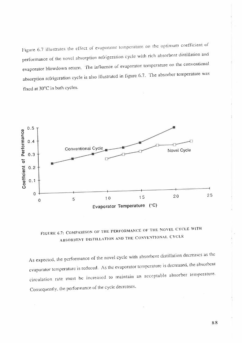
Figure6.Tillustratestheeffectofevaporatortell]peratureotltlreoptimumcoefficientof
performance of the novel absorption refrigeration cycle with rich absorbent distillation and
evaporator blowdown return. The influence of evaporatol temperature on the conventional
absorption refrigeration cycle is also illustrated in figure 6'7' The absorber temperature was
fixed at 30"C in both cYcles
Conventional CYcle Novel CYcle
0.5
0.4
(l)()c(5
Eooo-
oco'õ
ooo
0.3
1
0
0.2
0
10 15
Evaporator TemPerature ("C)
20 250
FIGURE6.7:COMPARISoNoFTHEPERFoRMANCEoFTHENovELCYCLEwIT}l
AßSORBENT DISTTLLATION AND THE CONVENTIONAL CYCLE
As expected, the performance of the novel cycle with absorbent clistillation decreases as the
evaporator temperature is recluced. As the evaporator temperature is decreased' the absorbent
circuration rate must be increased to maintain an acceptable absorber ternperature'
Consequently' the perfonnance of the cycle decreases'
5
88

Figure 6.7 also shows that tl-re perfonnance of the conventional cycle is superior to that of the
novel cycle with absorbent distillation. The reduced perforrnance of the novel cycle can be
explained by the low purity of the refrigerant from the liquid separation drum. Consequently, a
significant fraction of the available refrigeration duty is required to cool the large evaporator
blowdown stream to the evaporator temperature.
6.3.2 Cycle With Refrigerant Phase Rectification
A process flow diagram of the novel absorption refrigeration cycle with refrigerant phase
rectification is presented in figure 6.8. In this example, the evaporator and the absorber were
fixed at 15oC and 30oC respectively. The optimum reboiler temperature was 110"C.
Comparison with the conventional cycle, illustrated in figure 6.6, highlights the following
points:
(Ð The composition of the lean absorbent is considerably higher than that obtained in
simulations of the conventional cycle. This effectively limits the minimum evaporator
temperature which can be achieved. In order to lower the composition of the lean
absorbent, the fraction of absorbent sourced from the distillation column bottom product
must be increased. However, this can only be achieved by increasing the composition of
the rich absorbent exiting the absorber. Consequently, the desired increase in boiling
point elevation is diminished.
(iÐ The generator temperature is significantly higher than the generator temperature in the
conventional cycle. In the novel cycle with refrigerant phase rectification, the flowrate of
absorbent exiting the bottom of the distillation column is limited by the separation
achieved in the liquid phase sepa-ration drum. Consequently, a high generator temperature
is required to minimise the concentration of the combined lean absorbent stream.
89

2
Dury - 0.70 MW
I3
8
5
6 7
Absor
Duty= 1.22MW
DistillationColumn
ReboilerDutY = 6.96 ¡4Y¡
Rich AbsorbentRetum Pump
Power = 0.01 MW
4
Duty - 1.09 MW
9
CondenserDuty = 1 MW
RefluxDrum
Liquid
Vessel
Absorbent HeatRecovery ExchangerDuW - 2.18 À,fW
STREAMNO r23456789
Flowrate (kmol n-1¡
Composition (mol Vo)
Tempcrature ('C)
Pressu¡e (kPa)
Liquid Fraction
333
31.0
102.0
466.5
1.0
r28
96.4
30.0
146.6
1.0
t28
96.4
15.0
43.3
0.0s6
rt52
5.0
102.0
146.6
1.0
205
0.0
r 10.0
146.6
1.0
1351
4.2
101.3
466.5
0.992
1351
4.2
35.2
466.5
1.0
1485 1485
r2.2 r2.2
30.2 78.5
466.s 466.5
1.0 1.0
FIGURE 6.8: PROCIISS FLOW DIAGR^M OF THE NOVEL AIISORPTION REFRIGERATION
CYCLB WITH REFRIGERANT PHASE RECTIFICATION
90

o()c(u
EL
o(¡)
CL
oco'õ
oo()
(iii) Higher purity retì-igerant is ernployed in the novel cycle with refrigerant phase recrificario¡
cornpared with that used in the co¡rve¡rtional cycle. This is required to offset the
deleterious effect of the high lean absorbent concenffatron.
Figure 6.9 illustrates the influence of evaporator temperature on the optimum coefficient of
performance of the novel absorption refrigeration cycle with refrigerant phase rectification. The
performance of the conventional cycle is also illustrated in figure 6.9 to enable comparison.
The absorber temperature was fixed at 30'C in both cycles.
0.5
0.4
Conventional CycleNovel Cycle
0.3
0.2
0.1
0 10 15
Evaporator Temperature ("C)
20 25
FICURE 6.9: PERFORMANCE COMPARISON BETWEEN THE NOVEL CYCI,E WITH
REFRIGERANT PHASE RECTIFICAI'ION AND THE CONVIìNTTON^I- CYCLE
As expected. the perfonnance of the novel cycle with refrigerant phase rectiñcation decreases as
the evaporator temperature is reduced. This is because the absorbent circulation rate must be
increased to maintain the desired absorber tetnperature as the evaporator temperature is
decreased.
0
5
9l

While the performance of the novel cycle with refrigerant rectif,rcation is superior to that of the
novel cycle with absorbent distillation (see section 6.3.1), figure 6.9 shows that the best
performance is still obtained from the conventional cycle.
The reduced performance of the novel cycle with refrigerant rectification can be explained by
the inherent high concentration of refrigerant in the lean absorbent. Consequently, the
absorbent circulation rate or the refrigerant purity must be increased. Losses also result from
the mixing of the absorbent streams exiting the liquid separation d¡um and the distillation
column.
6.3.3 Cycle With Refrigerant Recovery from the Evaporator Blowdown
A process flow diagram of the novel absorption refrigeration cycle with refrigerant phase
rectification is presented in f,rgure 6.10. In this example, the temperatures of the evaporator and
the absorber were f,rxed at 15"C and 30"C respectively. The optimum reboiler temperature was
80.5'C. Examination of the stream data presented in figure 6.10 highlights the following
points.
(i) The cornbination of high purity fresh refrigerant from the distillation column and low
purity evaporator blowdown (necessary for subsequent liquid phase separation) ensures
that the flowrate of the evaporator blowdown stream is very small. Consequently, the
amount of extra refrigerant recovered using this flowsheet is minimal.
(iÐ The evaporator pressure is less than that obtained in the conventional cycle because of the
low purity of the evaporator blowdown. Consequently, the absorber pressure is low and
the required absorbent circulation rate must be high. This leads to poor performance.
The coefficient of performance of the cycle in this exarnple was 0.27, considerably worse than
that obtained frorn the other cycles. In view of the poor perf ormance, further investigations of
this cycle were abanclonecl.
92

7
d
Vessel
r\
>
RichRetum Pump
Power = 0.02 MW
DutY = 0.70 MW
Absorber
Cooler
Dury = 2.gg lvty
ReboilerDutY:2.61 MW
CondenserDutY=f.26MIV
DutY = ¡"t
Absorbent HeatRecovery ExchangerDuty = 1.26 ¡41Y
FIGURE 6.10: PROCESS FLOW DIAGRAM OF THE NOVEL ABSORPTION REFRIGERATTON
CYCLE WITH REFRIGERANT RECOVERY FROM THE EVAPORATOR BLOWDOWN
STREAMNO I 2 3 4 5 6 7 I 9 l0 1l
Flowrate (kmol h-l)
Composition (mol7o)
Temperature ('C)
Pressure ftPa)
Liquid Fraction
140
94.r
48.0
t46.6
1.0
t4t93.8
41.6
146.6
1.0
1.09
23.0
15.2
466.5
1.0
1.09
23.0
78.3
466.5
1.0
0.61
31.0
47.8
466.5
1.0
0.48
5.0
102
466.5
1.0
140
94.1
15. r
26.3
0.003
4548
0.83
80.s
146.6
1.0
4548
0.83
35.2
t46.6
1.0
4688
3.6
30.2
146.6
r.0
4688
3.6
10.1
146.6
1.0
93

6.4 Simplified Analvsis of Cycles With Trimethvlamine and Water
In chapter f,rve, low molecula¡ weight, tertiary amines were selected as candidate refrigerants in
the novel absorption refrigeration cycle, with water as the absorbent. In particular,
diethylmethylamine and dimethylethylamine were employed as refrigerants in simulations of the
basic novel absorption refrigeration cycle.
With the introduction of a distillation step to the novel cycle in this chapter, diethylmethylamine
was discarded as a refrigerant because of its high boiling point. In contrast, the difference
between the boiling point of dimethylethylamine and water was sufficient to enable the hybrid
novel absorption refrigeration cycles to be modelled and compared with the conventional cycle.
However, the performance of the conventional cycle employing dimethylethylamine and water
as the working fluid pair was considerably worse than the performance expected with
conventional refrigeranl absorbent pairs. Clearly, alternative refrigeranl absorbent pairs with a
greater difference in normal boiling point are required.
Unfortunately, there are very few alternative mixtures known to exhibit the required
thermodynamic behaviour for application in the novel cycles. Trimethylamine and water were
identified as one alternative refrigerant/ absorbent pair. While the boiling point of
trimethylamine is the lowest of all the tertiary amines (approximately 2oC), experiments showed
that liquid phase separation in trimethylamine - water mixtures could not be achieved unless salt
was added.
Unfortunately, these factors add significant complexity to the formulation of a suitable
thermodynamic prediction model for detailed analysis of the novel absorption refrigeration
cycles discussed above. In particular, experimental lirnitations prevented the aquisition of
sufhcient experimental data, at high temperatures, for the prediction of phase equilibria in the
distillation column. The addition of the third component also necessitates a more sophisticated
thermodynamic model such as that proposed by Tan and Ti (1989)
94

A more simplified analysis of the potential of rirnethylamine - water mixtures as candidate pairs
for application in absorption refrigeration cycles was devised. This analysis procedure was
employed to assess the merit of pursuing an extended experimental program. If the results of
this analysis were favourable, the commercial potential of this working fluid pair would be
considered sufficient to justify reconstruction of the experimental apparatus to obtain the
required experimental data for a more complete analysis.
6.4.1 Description of the Simplified Absorption Refrigeration Cycle Analysis.
The simplified analysis compares the ratio of lean absorbent flowrate to refrigerant flowrate in
absorption refrigeration cycles which employ trimethylamine/ water and ammonia,/ water as the
refrigerant/ absorbent pair. A high value for this ratio results in increased losses in the heat
recovery exchanger a¡rd the distillation column with concomitant poor cycle performance.
Assumptions made on the lean absorbent composition, refrigerant composition and evaporator
blowdown fraction are employed to eliminate the necessity for simulating the generator.
Calculations are based on an evaporator temperature of 4oC and an absorber exit temperature of
35'C. The flow sheet employed to simulate the absorbent/ refrigerant flow ratio is illustrated in
figure 6.1 1. The thermodynamic model used for predicting the phase equilibria of mixtures of
trimethylamine and water is described in chapter 4.
Figure 6.12 illustrates the influence of lean absorbent composition on the ratio of absorbent to
refrigerant flowrate for the two refrigerants trimethylamine and ammonia. Figure 6.12 shows
that the absorbent to refrigerant flow ratio for the absorption of trimethylamine into solution
with water is an order of magnitude greater than that obtained with ammonia and water.
Clearly, the trirnethylamine/ water working fluid pair will not cliallange the performance of the
conventional aqua - ammonia absorption refrigeration cycle.
95

The addition of salt to mixtures of trimethylamine and water is required to obtain liquid phase
separation in the novel absorption refrigeration cycles. However, the addition of salt reduces
the affinity between trimethylamine and water. For this reason, the addition of salt would
further increase the absorbent to refrigerant flow ratio.
On the basis of these findings it was decided not to pursue detailed phase equilibrium
experiments on mixtures of trimethylamine, water ard salt.
Refrigerant99.9 mol%o refrigerant27o liquid carryover4
Evaporator
Absorber
Coo n
Rich AbsorbentSaturated liquid35"C
Lean Absorbent2 to 10 mol%o refrigerant50'c
FIGURE 6.11: FLOW SCHEMATIC FOR DETERMINTNG THE ABSORBENT REFRIGERANT FLOW
RATIO
96

3otrc(u
(l)
.9q)o0cE
(Eofrco.c¡
oØ-c¡
BO
70
60
50
40
30
20
10
0
Trimethylamine/ Water
468Wt% Refrigerant in Lean Absorbent
2
Ammonia/ Water
10 12
FIGURE 6.12: THE INFLUENCE OF ABSORBENT COMPOSITION ON ABSORBENT
REFRIGERANT FLOW RATIO
97

6 .5 Conclusions
In this chapter a number of "hybrid" absorption refrigeration cycles were investigated which
include both a liquid phase separation step and a distillation step to separate refrigerant from the
rich absorbent returning from the absorber. The thermodynamic performance of these cycles
was modelled with the PROCESSTM chemical plant simulation package using
dimethylethylamine and water as the working fluid pair.
In one of these cycles, the absorbent phase exiting the liquid separation drum was passed to a
distillation column, where the bulk of the remaining refrigerant was stripped from the
absorbent. Optimum performance was obtained from this cycle when the liquid blowdown
from the evaporator was employed as reflux to the distillation column. Despite this
improvement, the low purity of the fresh refrigerant entering the evaporator resulted in reduced
performance compared with that obtained from the conventional absorption refrigeration cycle
employing the same absorbenl refrigerant working fluid pair.
The "hybrid" cycle with the best thermodynamic performance employed a distillation step to
recover absorbent from the refrigerant rich phase exiting the liquid phase separation drum.
Unfortunately, the purity of the lean absorbent, in this cycle, is limited by the composition and
flowrate of the absorbent phase exiting the bottom of the liquid separation drum.
Consequently, the boiling point elevation between the evaporator and the absorber is
significantly reduced compared with the conventional absorption refrigeration cycle.
A cycle can also be devised where refrigerant is recovered from the liquid blowdown exiting the
evaporator in a liquid phase separation step. However, the high purity of the refrigerant,
obtained from the conventional distillation column, severely limits the amount of refrigerant
which can be recovered. The thermodynamic performance of this cycle was significantly worse
than that obtained frorn the other cycles investigatecl.
98

The absorbent to refrigerant flow ratio, required in an absorption refrigeration cycle employing
the trimethylamine - water working fluid pair, was calculated over a range of lean absorbent
concentrations. The results of these calculations were compared with the results of similar
calculations with the conventional ammonia - water working fluid pair. This comparison was
used to demonstrate that the thermodynamic performance of absorption refrigeration cycles
employing trimethylamine and water would be insufficient to justify commercial application of
this absorbent/ refrigerant pair.
It is apparent from these results, that the application of a liquid phase separation step in an
absorption refrigeration cycle is unlikely to find commercial application in any form.
99

Chapter 7.
THB NOVEL ABSORPTION CYCLE HBAT.PUMP
In this chapter, a type II absorption cycle heat-pump is proposed. Thís cycle employs working
fluid pairs which exhibit "upper critica.l solutÌon temperature behnviour" to effect the separatíon
of volatile working fluid from the absorbent in a low temperature generator. A number of
variations to this cycle which include a distillation step are also proposed. Simulatíons of the
performance of each cycle are presented and the potential of these cycles is discussed.
In chapters 5 and 6, mixtures exhibiting lower critical solution temperature behaviour were
employed as working fluids in a series of novel absorption refrigeration cycles. Unfortunately,
low coefficients of perfonnance were predicted in simulations of these cycle with the working
fluid pairs known to exhibit the required thermodynamic behaviour. In view of the limited
number of mixtures which exhibit lower critical solution temperature behaviour, it is unlikely
that a more suitable alternative working fluid pair will be found.
In contrast, numerous binary mixtures exhibit upper critical solution temperature behaviour.
While such mixtures a-re unsuitable for the refrigeration cycles described in chapters 5 and 6,
they could find application in a heat pump cycle where volatile working fluid recovery occurs at
low temperature.
Figure 7.1 illustrates the direction of energy flow in the two possible types of absorption cycle
heat purnp. In this figure, the horizontal lines represent the temperature levels of the available
heat sources/ sinks, and the arrows represent the direction of the energy flow. Arrows pointing
into the line represent heat input to the cycle and arrows pointing out from the line represent
heat rejection. The type I cycle utilizes high - grade energy to raise the temperature of a low -
grade heat source. The useful heat from this process is rejected at an intenrediate temperature.
The type II cycle ernploys heat at an intermecliate temperature and rejects heat at both low and
high ternperatures.
100

Tz'Tr'To
/ / T2
T1
To
Type I Type II
FIGURE 7.1: DIRECTION OF ENERGY FLOW FOR THE TWO FEASIBLE HEAT PUMP TYPES
In this chapter, a type II heat pump is described which employs mixtures exhibiting upper
critical solution temperature behaviour as working fluids. The partial miscibility of these
mixtures at low temperature is utilized to separate the volatile working fluid from the rich
absorbent.
To demonstrate the feasibility of the proposed novel absorption cycle heat pump, cyclohexane
and aniline were chosen as candidate working fluids for computer simulation of the novel heat
pump. This pair was selected because of the large difference in boiling point between the two
compounds and the large composition range over which liquid phase separation occurs.
The thermodynamic performance of a number of cycle variations which include an additional
distillation step are also investigated. The performance of these cycles is compared and their
potential is discussed.
101

7.1 Description of the Novel Ahsorption Cvcle Heat PumI¡s
7.1.1 Basic Novel Type II Heat Pump
The novel type II heat pump cycle is illustrated in figure 7.2. In this cycle, the volatile working
fluid is partially boiled in an evaporator using low grade heat. The resulting vapour then
dissolves in a high boiling point absorption fluid with the heat of solution released at elevated
temperature. The rich absorbent is subsequently cooled until the volatile working fluid
becomes immiscible in the absorbent. The resulting two liquid phases are separated in a settling
drum, with the recovered volatile working fluid returned to the evaporator and the absorbent
phase passed to the absorber.
As the liquid phase separation is imperfect, the absorbent stream contains a fraction of the more
volatile component and a fraction of the less volatile absorbent remains in the working fluid.
Liquid is removed f¡om the evaporator and returned to the settling drum to prevent build up of
the less volatile component in the evaporator. Heat exchangers are employed to preheat the
absorbent and working fluid, and to simultaneously precool the settling - drum feeds.
Figure 7.3 details a flow schematic of a conventional type II absorption cycle heat pump for
comparison. In contrast to the conventional cycle, the novel cycle includes a liquid - liquid
separation drum in place of the conventional distillation column ancl blowdown from the
evaporator is recycled to the generator.
In an attempt to improve the thermodynamic performance of the novel heat pump, a number of
hybrid cycles including a distillation step were synthesized. The principal reason for the
additional distillation step is to increase the purity of the working fluids, thus reducing the
ci¡culation rates of the working fluids and increasing performance.
102

CirculationPump
Absorber
vaporator
Cooling heat releasetemperatuHigh
Lowtemperatureheat input
LiquidSeparationVessel
CirculationPump
FTGURE 7,2: FLOVI SCHEMATIC OF THE NOVEL TYPE II ABSORPTION CYCLE HBAT PUMP
r03

Reflux
[,ow temperatureHeat input
Evaporator
Condenser
Cooling Hightemperatureheat rejection
DistillationColumn
[.owTemperatureHeat input
CirculationPump
Ci¡culationPump
FIGURE 7.3: FLOW SCHEMATIC OF THE CONVENTIONAL TYPE IIABSORPTION CYCLE HEAT PUMP
r04
7.1.2 Novel Type II Heat Pump With Absorbent Phase Distillation
The novel absorption cycle heat pump with absorbent phase distillation is illustrated in figure
7.4. In this cycle, volatile working fluid present in the absorbent phase exiting the liquid
separation drum, is stripped in the distillation column. The overheads from the distillation
column are condensed and combined with the volatile working fluid phase exiting the liquid
separation drum. The resulting stream is pumped to elevated pressure and passed to the
evaporator. Blowdown from the evaporator is used as reflux to the distillation column. This
cycle is a corollary of the refrigeration cycle illusfrated in figure 6.2.
7.I.3 Novel Type II Heat Pump With Volatile Phase Rectification
Figure 7.5 illustrates an alternative heat pump cycle in which the volatile working fluid phase
exiting the liquid separation drum is distilled to recover lean absorbent. The rich absorbent fi¡st
enters the liquid phase separation drum where the volatile working fluid is removed from the
absorbent. The volatile working fluid stream is then passed to a distillation column containing
both rectification and stripping sections. A pure stream of volatile working fluid is recovered
from the top of the column and lean absorbent is removed from the bottom of the column. The
lean absorbent from the bottom of the distillation column is then combined with the absorbent
stream exiting the liquid sepa-ration drum and passed to the absorber. This cycle is a corollary
of the refrigeration cycle presented in hgure 6.3.
l0s

LiquidSeparatÍVessel
AbsorbentPhase
ndenser
Evaporator
Absorber
UsefulHeat R
DistillationColumn
HeatInput
AbsorbentCirculationPunrp
FIGURE 7.4: FLOW SCHEMATIC OF THE NOVEL TYPE II ABSORPTION CYCLE
HEAT PUMP WITH ABSORBENT PHASE DISTILLATTON
106

Liquid
Vessel
Condenser
FIGURE 75: FLOW SCHEMATIC OF THE NOVEL TYPE II ABSORPTION CYCLE
HEAT PUMP WITH VOLATILE WORKING FLUID RECTIFICATTON
aporator
Absorber
UsefulHeat
DistillationColumn
HeatInput
107

7.I.4 Novel Type II Heat Pump With Volatile Working Fluid Recovery From
the Evaporator Blowdown
Figure 7.6 illustrates an alternative novel absorption cycle heat pump in which volatile working
fluid in the evaporator blowdown is partially recovered in a liquid phase separation step. The
blowdown stream exiting the evaporator is cooled by heat exchange with the fresh volatile
working fluid stream. It is then passed to the liquid phase separation drum where it is cooled
until phase separation occurs. The volatile working fluid phase is returned to the evaporator
and the absorbent rich phase exiting the liquid separation drum is passed to the absorber. This
cycle is a corollary of the refrigeration cycle illustrated in figure 6.4.
108
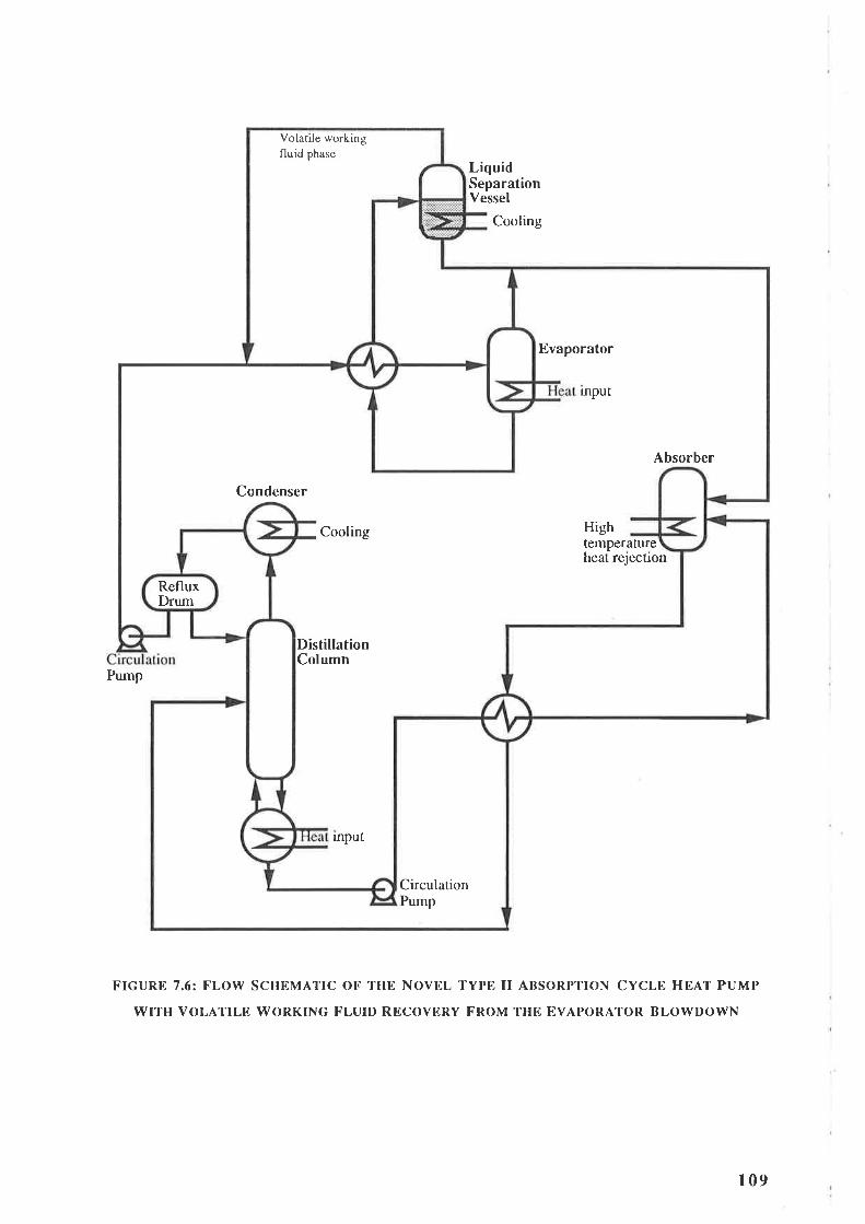
LiquidSeparationVessel
Cooling
Pump
FIGURE 7.6: FLOW SCHEMATIC OF THE NOVBL TYPE II ABSORPTION CYCLE HEAT PUMP
WITH VOLATILB WORKTNG FLUID RECOVERY FROM THE EVAPORATOR BLOWDOWN
Volatile workingfluid phase
RefluxDrum
Evaporator
mput
Absorber
Condenser
Cooling Hightemperatureheat rejection
DistillationColumn
input
CirculationPump
109

7.2 Selection of Working Fluids
Working fluids suitable for application in this cycle must exhibit upper critical solution
temperature behaviour upon mixing. As well, the selected pair should possess properties
which are desirable in conventional absorption cycle heat pumps. Properties of particular
importance include thermal stability and low corrosivity. A large difference between the boiling
point of the volatile working fluid and the absorbent is also desirable to ensure sufficient boiling
point rise in the absorber.
To demonstrate the feasibility of the proposed novel absorption cycle heat pump, cyclohexane
and aniline were chosen as candidate working fluids for computer simulation of the novel heat
pump and its variants. This pair was selected because of the large difference in boiling point
between the two compounds and the large composition range over which liquid phase
sep¿ì-ration occurs.
Conveniently, a large body of experimental data is available for the development of an accurate
thermodynamic model for mixtures of cyclo-hexane and aniline (Abello et. al., 1968, Hosseini
and Schneider, 1963, Korteum and Freier, 1954, Roeck and Sieg, 1955, Buchner and Kleyn,
1924, and Hunter.and Brown , 1947). The five - parameter NRTL model described in chapter
4 was used to predict the phase behaviour of these mixtures. By comparison of model
predictions and experimental data, the thermodynamic model was shown to predict mixture
vapour pressure with an average accuracy of +I.87o.
I t0

7.3 Computer Simulation of the Novel Heat Pump Cvcles
The performance of each of the proposed heatpurnp cycles was simulated with the
PROCESSTM che*ical plant simulation package. An approach temperature of 2 K was
assumed for the two heat recovery heat exchangers in the basic cycle. Larger approach
temperatures were not used for this cycle because of the low boiling point elevation achieved
between the evaporator and the absorber. The approach temperature was increased to 5 K for
simulations of the heat pump cycles which included the additional distillation step. In all
simulations, the temperature in the liquid phase separation drum was fixed at 25"C.
To obtain optimum performance from each cycle, the absorbent flowrate was adjusted to ensure
that rich absorbent exiting the absorber remains a saturated liquid. In addition, the f¡action of
working fluid boiled in the evaporator was optimised. This procedure is described in more
detail in section 5.3.3.
Heat pumps are generally employed to raise the temperature of an available low grade heat
source. Vy'aste heat from low pressure steam, at a temperature slightly in excess of 100oC, is
one common source of low grade heat. For this reason, the evaporator temperature was fixed
at 100oC and the influence of absorber exit temperature on cycle perforrnance was investigated.
The performance of the novel absorption cycle heat pumps was then compared with the
performance of the conventional absorption cycle heat pump ernploying cyclohexane and aniline
as working fluids.
The simulation procedure and simulation constraints parallel the detailecl discussion presented in
chapters 5 and 6.
tll

7.4 Simulation Results
7.4.1 Basic Novel absorption Cycle Heatpump
Simulations were conducted on the basic novel absorption cycle heat pump over a range of
absorber temperatures and with the evaporator temperature fixed at 100"C. A process flow
schematic of this cycle is presented in figure 7.8 with the absorber temperature fixed at 106oC.
Examination of the stream data, presented in the flowsheet, highlights the following points:
(Ð The boiling point elevation achieved between the evaporator and the absorber is very small
despite the large concentration difference between the absorbent and the volatile working
fluid. At the low temperatures experienced in the liquid phase separation drum, the boiling
point of the absorbent and the volatile working fluid must be identical if liquid phase
separation is to occur. However, the small difference between the boiling point of these
streams, at the elevated temperatures experienced in the evaporator and the absorber,
highlights the relative insensitivity of the shape of the cyclohexane - aniline phase envelope
to increasing temperature.
(ü) In order to increase the boiling point elevation between the evaporator and the absorber a
large fraction of the volatile working fluid must be recycled to the liquid phase separation
drum.
Figure 7.7 illustrates the influence of absorber temperature on the optimum coefficient of
performance for the basic novel absorption cycle heat pump. Performance falls dramatically as
the absorber temperature is increased until the cycle ceases operation with an absorber
temperature in excess of 108oC.
tt2

The reduction in perforrnance with increasing absorber ternperature can be attributed to the
increased circulation rate of absorbent required to dissolve the volatile working fluid. The
maximum absorber exit temperature corresponds to the saturation temperature of the lean
absorbent. At this temperature, the lean absorbent cannot absorb any vapour from the
evaporator.
0.1
103 104
0.3
o.2
(uIc{
¡r-oq)
o
q)
I
c)
(J
0.6
0.5
0.4
105 '1 06
Absorber Temperature (oC)
107 108
FIGURE 7.7: THE INFLUENCE OF ATISORBER EXIT TEMPERATURIi ON THE PERFORMANCE
OF THE NOVEL AIISORPTION CYCI.Iì HEAT PUMP
t l3

54
2
1
J
Evaporator BlowdownHeat Recovery Exchanger
Duty = 1.9
8
9
6
Absorber
Hieh
vaporator
Duty - 0.7 MWheat release
Ci¡culationPu¡np
Heat inputDuty = 1.78 MW
LiquidSeparationVessel
CoolingDuty = 1.08 MW
CirculationPump
Absorbent HeatRecovery ExchangerDuty = 10.32 MW
STREAMNO 123456189
Flowrate (kmol h-l)
Composition (mol7o)
Temperature ('C)
Pressure (kPa)
Liquid Fraction
988
87.0
25.0
164.7
1.0
988
87.0
88.2
164.7
1.0
840
85.1
100.0
t&.1
1.0
840
85.1
27.0
164.7
1.0
148
97.5
100.0
164.7
0.0
2881
2',7.0
25.0
t&.7
1.0
288r
21.0
104.0
t&.1
1.0
3030
30.s
106
t64.1
1.0
3030
30.s
32.6
164.7
1.0
FIGURIì 7.8: PROCESS F-I,OW DIAGRAM OF THE NOVEL ABSORPTION CYCLE HEAT PUMP
rt4

7.4.2 The Novel Type II Heat Pump With Absorbent Phase Distillation and
the Novel Type II Heat Pump With Volatile Phase Rectification
Despite the acldition of the distillation step in these cycles, the temperature range over which the
heat pump can operate is severely constrained when cyclohexane and aniline are employed as
working fluids. This is best illustrated by the phase diagram presented in figure 7.9. The
bubble point curve presented in this figure was calculated at a constant pressure of 167.5 kPa.
Assuming the evaporator temperature is 100oC, this pressure is approximately equal to the
pressure expected in the evaporator and absorber of these novel heat pump cycles.
In these two cycles, the rich absorbent exiting the absorber is separated into two phases in the
liquid separation drum. Consequently, the concentration of cyclohexane in the rich absorbent
stream must be between 2l mol%o and 87 mo|%o. Thus, from figure 7.9/- -.,
weþan deduce thatthe /boiling point elevation befween the evaporator and the absorber is limited to approximately 8.5
degrees C for these working fluids. This is significantly less than the boiling point elevation
which can be achieved in the conventional cycle (see section 7.4.3). For this reason, no further
simulations were conducted to determine the performance of these cycles.
From figure 7 .9, we can also see that the boiling point in the evaporator is quite insensitive to (
the composition of the evaporator liquid blowdown. Consequently, the evaporator pressure
can not be variecl significantly without influencing the evaporator temperature.
115

(-)o
q,)¡r
crú¡rq)Èq)F
250
50
200
150
100
0
0 0.2
Pressure = 167 kpa
0.4 0.6
Cyclohexane Concentrat¡on
0.8
FIGURE 7.9: CALCULATED BUBBLE POINT CURVE FOR MIXTURES OF
CYCLOHEXANE AND ANILTNE AT 167.5 KPA
rt
I l6

7 .4.3 The Novel Type II Heat Pump With Volatile Working Fluid Recovery
From the Evaporator Blowdown
Simulations were conducted on the novel cycle with volatile working fluid recovery from the
evaporator blowdown over a range of absorber temperatures and with the evaporator
temperature fixed at 100"C. A process flow diagram of this cycle is presented in figure 7.10
with the absorber temperature fixed at 120'C. A process flow diagram of the conventional type
II absorption cycle heat pump under the same conditions is also provided in figure 7.11 for
comparison. Examination of stream data, presented in these flowsheets, highlights the
following points:
(Ð The evaporator pressure in the novel cycle is significantly lower than that obtained in the
conventional heat pump. This low evaporator pressure is required to achieve an
appropriate concentration of cyclohexane in the evaporator blowdown to enable subsequent
purification in the liquid phase separation drum.
(ü) In the novel cycle, the distillation column overhead stream contains a lower concentration
of the more volatile component. At tlre higher distillation column overhead concentrations,
the optimum liquid blowdown concentration is too rich in cyclohexane to achieve liquid
phase separation. At the lower concentrations, however, the benefit of the liquid phase
separation step is increased because a larger fraction of the evaporator blowdown must be
recycled.
(iü) The concentration of the rich absorbent returning to the distillation column is higher in the
conventional distillation column. This results from the increased pressure in the evaporator
(and hence absorber) as previously discussed. The high concentration of the rich
absorbent enables reduced absorbent circulation rates and improved performance in the
conventional cycle.
tt7

LiquidSeparationVessel
Dury =0.03 MW
Pump
Absorbent HeatRecovery ExchangerDuty = 9.39 Ilv[W
FIGURE 7.10: PROCESS FLOW DIAGRAM OF THE NOVEL ABSORPTTON CYCLE HEAT PUMP
WITH VOLATILB WORKTNG FLUID RECOVBRY FROM THE EVAPORATOR BLOWDOWN
l=
Reflux
Evaporator
Evaporator BlowdorrninputHeat Recovery Exchanger
DutY = 0.47 M'W Duty = 2.46 ¡4Yr'
Absorber
Condenser
High
= 2.93 MW heat rejectionDury = 0.7 MW
Distillationumn
Heat input
Duty = 1.2 ¡4'¡Y
Ci¡culation
STREAMNO t 2 3 4 s 6 7 8 9 t0 ll
Flowrate (kmol n-1¡
Composition (mol Vo)
Temperature ("C)
Pressure (kPa)
Liquid Fraction
215
96.0
25.2
173.3
1.0
350
92.5
25.0
164.7
r.0
3-50
92.5
54.7
164.7
1.0
210
97.5
100.0
r&.7
0.0
140
8s.0
r00.0
164.7
1.0
136
87.0
25.0
t64.7
1.0
2t5
96.0
100.8
t64.1
0.037
t324
16. l
r20.0
t64.1
1.0
t324
r6.l
107.8
t64.7
r.0
I 109
0.1
r00.0
r73.3
1.0
1 109
0.7
I15.0
t73.3
1.0
118

2
1
RefluxDrum
3
5 6
4
I-ow temperatureHeat input
Duty = 2.32 ¡1Y¿
Absorber
Condenser
High
DutY = 2.78 MW heat rejectionDuty = 9.7 ¡41ry
DistillationColumn
DutY = L16 MW
CirculationPump
Pump
Absorbent HeatRecovery ExchangerDutY = 6.31 ¡4Y¿
STREAMNO 123456
Flowrate (kmol n-l;
Composition (mol Vo)
Temperature ("C)
Pressure (kPa)
Liquid Fraction
202
98.6
25.2
173.3
1.0
202
98.6
100.0
170.5
0.001
1203
t7 .t
120.0
170.5
1.0
1203
t] .l
t07.9
170.5
1.0
t00l
0.7
100.0
r73.3
1.0
1001
0.7
1r5.0
t73.3
1.0
FIGURE 7.II: FLOW DIAGRAM OF THE CONVBNTIONAL ABSORPTION CYCLE HBAT PUMP
tt9

Figure 7.12 illustrates the influence of absorber temperature on the optimum coefficient of
performance for the novel absorption cycle heat pump with volatile working fluid recovery
from the evaporator blowdown. Performance curves are provided for three distillation column
pressures of 95 mm Hg, 95.5 mm Hg and 96.5 mm Hg. As the condenser exit temperature
was fixed at25"C in all simulations, these distillation column pressures correspond to overhead
cyclohexane compositions of 96.027o,97.01Vo and98.397o respectively. The evaporator and
distillation column reboiler temperatures were fixed at 100"C in all simulations.
When the distillation column pressure was set to 96.5mmHg, the optimum liquid blowdown
from the evaporator was too rich in cyclohexane to achieve any liquid - phase separation.
Hence, the results given at this pressure are essentially those for a conventional absorption
cycle heat pump employing cyclohexane and aniline as the working fluids.
From figure 7 -12, it is evident that cycle performance decreases with increasing absorber
temperature. However, the temperature elevation achieved in the absorber of this cycle is
considerably geater than that achieved in the basic novel absorption cycle heat pump and cycle
performance is less sensitive to the absorber temperature.
Despite the liquid - phase working fluid recovery step, increasing overhead volatile composition
yields improved performance. Indeed, cycle performance continues to increase when the liquid
phase separation step becomes redundant at higher column pressure. This can be attributed to
the increased absorber pressure obtained with the higher overhead volatile compositions.
r20

(uIcË
-o¡i(u
O(
q)
I
q)o
(.)
0.4
0.3
A0.35
0.25
Column Overheads Compositionr Xcyclohexane = 96.0ZVo
! Xcyclohexane = 9i.\lVo
A Xcyclohexane = 98.3gEo
0.2
0.1 5
104 108 112 116 120 124Absorber Temperature (oC)
FIGURE 7.12: THE INFLUENCE OF ABSORBER TEMPERATURE ON THE PERFORMANCE OFTHE NOVEL ABSORPTTON CYCLE HEAT PTJMP WITH VOLATILE WORKTNG FLTIID RECOVERY
FROM THE EVAPORATOR BLOWDOWN
t2t
7.5 Conclusions
In this chapter, a novel type II absorption cycle heat pump, which employs a liquid phase
separation step to recover the volatile working fluid from the absorbent, was investigated.
Va¡iants of this cycle, which include an additional distillation step, were also analysed. The
thermodynamic performance of these cycles was modelled with the PROCESSru chemical plant
simulation package using cyclohexane and aniline as the working fluid pair.
Results of simulations on the basic novel type II absorption cycle heat pump demonstrated that
only a small increase in temperature between the evaporator and the absorber could be achieved
with the selected working fluid pair. This was attributed to the relative insensitivity of the
shape of the cyclohexane - aniline phase envelope to increasing temperature.
With the addition of a distillation step, the purity of either the volatile working fluid or the lean
absorbent can be increased. In two such cycles, the rich absorbent exiting the absorber is
cooled and passed to the liquid phase separation drum. Either the volatile working fluid phase
or the absorbent phase exiting this drum can then be distilled to improve stream purity.
Unfortunately, only small improvements were made to the boiling point elevation between the
evaporator and the absorber, in these cycles. Further increases in the boiling point elevation
could only be achieved by decreasing the concentration of cyclohexane in the rich absorbent
stream. However, this would make phase separation in the liquid phase separation drum
impossible.
The most effective of the novel heat pump cycles, employed the liquid phase separation step to
recover refrigerant from the liquid blowdown exiting the evaporator. Primary separation of
volatile working fluid from the rich absorbent was achieved in the distillation column. In this
cycle, the purity of the volatile working fluid entering the evaporator must be low to obtain
significant volatile working fluid recovery in the liquid phase separation drum. This results in
Iow thermodynarnic performance when cornpared with the conventional type [I absorption cycle
heat purnp ernploying the sarne working fluid pair.
122

Chapter 8.
BVAPORATOR BLOWDOWN RBCYCLE IN A CONVBNTTONAI.
AQUA AMMONIA ABSORPTION REFRIGERATION CYCLE
ln previous chapters, recycling of the evaporator liquid blowdown to the generator was
introduced as a means for reducing performance losses which result from poor refrigerant purity.
In this chnpter, the principle of returning liquid blowdown from the evoporator to the generator is
applied to the conventional aqun - ammonia absorption refrigeration cycle. In this application, the
returning liquid can be used as reflux to the distillation column, thus eliminating the necessity for
fresh refrigerant reflux. The performance and cost of the cycle with evûporator blowdown return
is compared wíth that of the conventional cycle. The commercial potential of the new cycle is
discussed.
In chapters 5 and 6, a series of novel absorption cycle refrigerators were devised which include
evaporator blowdown recycle to the generator. The application of evaporator blowdown recycle
was found to be particularly attractive in these cycles because of the poor purity of the refrigerant.
The recycle effectively reduces the load on the absorber and increases thermodynamic
performance.
In conventional absorption refrigeration cycles employing a volatile absorbent, (e.g. organic
solvent or water) some fraction of absorbent is carried over into the refrigerant. The absorbent is
concentrated in the liquid phase in the evaporator, thus limiting the quantity of refrigerant which
can be evaporated. This problem can be reduced by improved rectification in the distillation
column. However, the increased duty in the generator which is required to improve product
purity may negate any benefit from the reduction in required liquid blowdown. For the aqueous-
ammonia system, a refrigerant purity of approximately 99.97o ammonia appears to be close to the
optimurn (Bogart, 198 1).
r23

A number of alternative cycles have been suggested for reducing the quantity of liquid blowdown
from the evaporator. One cycle employs a partial condenser (dephlegmator) to produce reflux to
the distillation column. Any absorbent "carry-over" in the vapour overheads is preferentially
condensed in the partial condenser. The resulting higher purity vapour is then passed to the total
condenser to form fresh liquid refrigerant feed to the evaporator. This cycle is illustrated in figure
2.2.
Another cycle employs the principle of resorption. By recirculating liquid from the evaporator,
the concentration of the liquid phase in the evaporator can be controlled so that the equilibrium
vapour phase composition is equal to that of the fresh refrigerant. In theory, one hundred percent
of the fresh refrigerant can be vaporised in this cycle and improved performance is obtained.
Cycles have been devised which employ a pump to enable the evaporator blowdown to be added
downstream of the rich absorbent return pump (Bogart, 1981). However, the concept of
replacing fresh refrigerant reflux to the distillation column with the returning liquid evaporator
blowdown stream does not appear to have been proposed in the literature. This is surprising as
the presence of absorbent contamination in the refrigerant stream is evidence of the potential for
this approach. In conffast to the other cycles discussed in the previous paragraphs, this cycle
does not minimise the fraction of fresh refrigerant appearing as liquid blowdown from the
evaporator. Instead, the size of the liquid blowdown stream is controlled to ensure sufficient
reflux to the distillation column.
Application of this concept to the conventional aqua - ammonia absorption refrigeration cycle
appears to be attractive and worthy of further investigation. For this reason, the performance and
cost of the aqua - arnmonia absorption refrigeration cycle with evaporator blowdown reflux, was
investigated in detail. In this chapter, the results of this investigation are presented. Simulation
results are compared with the conventional aqua - ammonia absorption refrigeration cycle and the
potential of the modified cycle is discussed.
124

8.1 Cycle Description
In the conventional absorption refrigeration cycle (figure 2.1), high purity refrigerantfrom the
distillation column is condensed and collected in a reflux drum. A portion of this refrigerant is
returned to the column as reflux and the rest is passed to the evaporator to provide useful
refrigeration. Any absorbent contamination in the refrigerant is removed from the evaporator as a
liquid by entrainment or blowdown.
Spent refrigerant vapour from the evaporator is dissolved/condensed in the absorption fluid and
the resulting refrigerant rich absorbent is pumped to high pressure where the refrigerant is
recovered from the absorbent by distillation.
If limited waste heat is available or if the heat supplied is valuable, fuel can be conserved by
precooling the liquid refrigerant with spent refrigerant vapour from the evaporator (f,rgure 8.1).
The modified cycle eliminates the use of refrigerant exiting the condenser as reflux to the
distillation column. However, rectification is still achieved in the distillation column by returning
liquid blowdown from the evaporator to the top of the column (figure 8.2). If required,
precooling of the refrigerant can be achieved by heat exchange with the evaporator blowdown
(figure 8.3) and by heat exchange with spent refrigerant vapour exiting the evaporator (figure
8.4).
In conventional designs, the liquid phase in the evaporator contains the bulk of any absorbent
which was carried over from the distillation column. The presence of the absorbent reduces the
fraction of the fresh refrigerant which can be boiled in the evaporator, with consequent reduction
in performance. In the case of the aqua - ammonia cycle, the resulting liquid removed from the
evaporator contains large quantities of ammonia refrigerant (approx 90Vo) whích can not provide
useful refrigeration. If the evaporator blowdown is passed to the absorber, additional absorbent
is required to dissolve the additional refrigerant.
t25

Useful refrigeration is also lost in conventional designs by using fresh refrigerant as reflux to the
distillation column. In the modif,red cycle, the entire refrigerant stream is passed to the evaporator
so that the maximum amount of refrigeration can be obtained per unit of column vapour
overheads. In this way, only spent refrigerant is used as reflux to the distillation column. The
combination of condenser and evaporator in the modified cycle could be viewed as a partial
condenser for the distillation column.
126

\7
)>\-/
RefluxDrum
Condenser
Absorber
Refrigeration
Evaporator
Reboiler
DistillationColumn
FIGURE 8.I: CONVENTIONAL ABSORPTION REFRIGERATION CYCLE
WTTH REFRICERANT PRECOOLING
t27

EvaporatorBlowdown Rec
Evaporator
Reboiler
RectificationSection
StrippingSection
Absorber
Con
DistillationColumn
FIGURE 8.2: ABSORPTTON REFRIGERATION CYCLE WTTH
EVAPORATOR BLOWDOWN RBTURN
t28

RecycleEvaporatorBlowdown
Reboiler
DistillationColumn
Absorber
Condenser
Evapor
RefrigerantPrecooler
FIGURE 8.3: ABSORPTION REFRIGERATION CYCLE WITH EVAPORATOR
BLOWDOWN RETURN AND PARTIAL REFRIGERANT PRECOOLING
r29

Evaporator
Li
on
Vapour PhaseRefrigerant
id Phasegerant Precooler
Reboiler
DistillationColumn
Absorber
EvaporatorRec
Condenser
FIGURE 8.4: ABSORPTION REFRIGERATION CYCLE WITH EVAPORATOR
BLOWDOWN RETURN AND FULL REFRIGBRANT PRECOOLING
130

8.2 Computer Simulation of the Modified Cycle
Process simulations were conducted to assess the impact of recycling the evaporator blowdown
on the performance and cost of the aqua-ammonia absorption refrigeration cycle. These
simulations were conducted on the PROCESSTM computer simulation package using the equation
of state proposed by Ziegler and Trepp (1984) for predicting the thermodynamic properties of
ammonia - water mixtures.
Clearly, there a¡e a number of cycles which could have been chosen for comparison with the
modified cycles illustrated in figures 8-2 to 8.4. The conventional cycle (figure 2.1) and the
conventional cycle with refrigerant precooling (frgure 8.1) were chosen for comparison. With the
exception of the proposed modification, these cycles are identical to the modified cycle.
To ensure accurate comparison, all simulations were based on an absorber exit temperature of
44oC and a condenser temperature of 44"C. The generator temperature and the approach
temperature in each of the heat recovery heat exchangers were varied to ensure that optimal
performance was achieved. For the two conventional cycles, the evaporator liquid blowdown
rate was also optimised.
In most simulations, the cycle was optimised by minimising the cost of the required heat
exchangers at a fixed refrigeration duty of 0.69MW. This objective was chosen to reflect a
scena¡io where cycle performance is of secondary importance, applicable when the cycle is fired
by waste heat of low value. The use of total heat exchanger cost was chosen in place of the
overall refrigerator cost to reduce calculation complexity. Experience has shown that this criteria
can be used for comparitive estimation of total investment expenditure (Holldorf, 1979).
The heat exchanger cost equation ernployed in this study (Linhoff and Ahmad, 1990) is presented
as equation 8.1. Additional assumptions used in the cost analysis are surruna-rised in table 8.1.
Cosr = $10,000 + 350 area (rn2) .....(S.1)
131

-2 -l50Wm KOverall Heat Transfer Coefficient
@e fri geran t Vapour Heatin g)
Overall Heat Tr¿nsfer Coefficient(Other Exchangers)
Available Stearn Temperature
Refrig. Vapour Superheater Pressure Drop
Distillation Theoretical Plates
2K
I1000 V/ m
170'c
12 kPa
5
TABLE 8.1: ASSUMPTIONS IN THE CYCLE COST ANALYSIS.
Further discussion on the simulation procedure and simulation constraints is detailed in chapter 5
The validity of the conventional aqua-ammonia absorption refrigeration cycle PROCESS model
was tested by comparing the value of a number of key parameters calculated by the model with
those obtained by other authors. The results of this comparison are presented in table 8.2.
Vaiues obtained from the PROCESS model appeil to compare well other designs from the
literature.
Sour.cp Tu.,ro" Xu-Assonse|ìT/REFzuGERAÀTT
RA1]O
T{EFLUXRATIO
NOTES
Ludwig (1965)
Bogart (1981)
Bogart (1981)
Bogart (1981)
Bogaf (1981)
Bogart (198 1)
V/hite
No account of blowdown
Maximised heat recovery
Low temp. heat source
Dual evaporator
High value heat sou¡ce
High temp. heat source
This work (fig 8.5)
-15'c5.6'C
-29"cl6"c & 1.7'c
-20"c
-3.9"C
-10"c
25.8 wTTo
29.4 wt%o
17.4 w¡Vo
30.0 wt%o
25.0 wtVo
20.0 wÍ%o
l8.l wt%o
0.5- 1.0
0.1 l
0.1-5
0. l0
0.41
0.15-0.36
0.32
7.4r
r.97
6.0s
1.1'7
6.50
3.04
3.68
TATLE 8.2: COMPARISON OF THE CONVENTIONAL AMMONIA WATER ABSORPTION
RBFRTGERATION CYCLE MODEL WITH OTHT]R I,ITERA-I'URE DESIGNS
r32
8.3 Case Study of the Modifred Cvcle
Ammonia water absorption refrigeration has been successfully employed in ammonia
manufacturing plants. In one application 12.6 MV/ (3580 tons) of refrigeration was required at
-10oC (Holldorf, 1979). As a case study for comparison of the new technology, conventional
and modified absorption refrigeration cycles were designed for this application. Design
assumptions were similar to those discussed in section 8.2 except that the distillation column was
increased to 7 theoretical stages and the cost objective function was altered to account for
operating costs. Operating cost were calculated from the required cooling water valued at
US$0.05 / tonne ($0.tq / 1000 gallon).
Process flow diagrams, including a complete listing of sffeam conditions, are presented in figures
8.5 and 8.6 for the optimised conventional and modified cycles with partial refrigerant
precooling. Technical comparison of the two cycles highlight the following points:
(Ð The required absorbent flowrate is lowered in the modified cycle. This results from the
increased evaporator (and hence absorber) pressure.
(iÐ The apparent reflux ratio is marginally reduced in the modified cycle. However, the actual
reflux in the column is higher for the modif,red design as the returning reflux is sub-cooled.
The increased actual reflux rate results from the lower ammonia composition in the modified
cycle reflux stream.
(üi) The reflux return pump duty has a negligible effect on the COP in both designs
(iv) Evaporator blowdown accounts for 23.97o and 5.27o of the evaporator feed in the modified
and conventional designs respectively. The increased evaporator blowdown flowrate is
required to maintain the optirnum reflux flow-rate to the distillation column.
133

Bvaporator
Duty = 12.6
I
RefluxDrum
Evap. Blowdown Reci¡c.
Power =
CondenserDuty = 19.3 MW
Absorber Recirc.Pump Power = 0.2 MW
11
Duty = 28.4 MWoiler
DistillationColumn
t2
AbsorberDuty - 21.8 MW
Srns,cMNo 123456 '1 89 l0 11 t2
Flow (kmol h-l)
Conc. (mol %)
Temperature ('C)
Pressure (atm)
HeatFlow (MW)
Liquid Fraction
3552
99.7
63.6
t7 .r,|
0.0
853
99.7
44.O
t'7 .t
0.84
1.0
2699
99.7
4t.6
r7 .t
2.5r
1.0
2559
100.0
-10.0
2.7 L2
15. 17
0.0
140
94.3
-9.4
t1 .l-0.06
1.0
t2032
36.72
6't .4
2.7 t2
19.22
0.831
12032
36.72
44.O
2.592
-2.61
1.0
140
94.3
40.0
t1 .l
0.10
1.0
t2t12
37.38
45.r
t1.t
-2.33
1.0
t2t72
37 .38
113.9
t7 .t
t7 .o2
1.0
947 4
19.6
r52.6
t7 .l
23.4
1.0
947 4
19.6
5 9.5
L7 .t
4.06
t.0
FIGURE 8.5: CONVENTIONAL CYCLE WITH PARTIAL REFRÍGERAN.I PRECOOLTNG
r34

CondenserDutY = 18.4 MW
=0.01 MWEvaporatorPump
Column
Absorber Recirc.Pump Power = 0.17 MW
ReboilerDuty - 26.4lvtlv Absorber
Duty = 20.8 MV/
1
Evaporator
Refrigeration
Duty - 12.6 MW
STREAMNO 123456189 l0 11
Flowrate (kmol h-l)
Concentraúon (mol %)
Temperature ('C)
Pressure (atm)
HeatFlow (MW)
Liouid Fraction
3378 807
99.10 98.78
32.3 -9.4
17.05 11.t
2.4t -0.20
1.0 0.0
3378
99.70
63.s
17.05
2r.10
0.0
33'78
99.70
44.0
17.05
3.34
1.0
807
98.78
4r.1
l1 .r
0.13
r.0
2510
100.0
-10
2.83r
15.22
0.0
l16l I
37.45
67.0
2.83t
18.20
0.831
r l61l
37.45
44.0
2.1tt
-2.58
1.0
1161 I
37.45
r r4.6
t] .r
16.93
1.0
9041
19.67
t52.5
17.05
22.31
1.0
9041
19.61
54.9
17.05
2.98
1.0
FTGURE 8.6: MODIFIED CYCLE WITH PARTTAL REFRIGERANT PRECOOLTNG
135
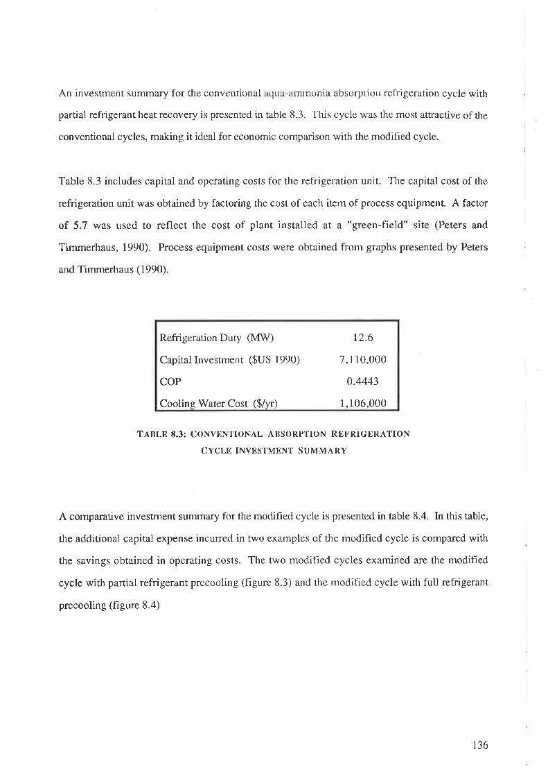
An investment summary for the conventional aqua-ammonia absorption refrigeration cycle with
partial refrigerant heat recovery is presented in table 8.3. This cycle was the most attractive of the
conventional cycles, making it ideal for economic comparison with the modihed cycle.
Table 8.3 includes capital and operating costs for the refrigeration unit. The capital cost of the
refrigeration unit was obtained by factoring the cost of each item of process equipment A factor
of 5.7 was used to reflect the cost of plant installed at a "green-field" site (Peters and
Timmerhaus, 1990). Process equipment costs were obtained from graphs presented by Peters
and Timmerhaus (1990).
Refrigeration Duty O,tW)
Capital Investment ($US 1990)
COP
Cooling Water Cost ($/l,r)
12.6
7,110,000
0.4443
1,106,000
TABLE 8.3: CONVBNTIONAL ABSORPTION REFRIGERATION
CYCLE INVBSTMENT SUMMARY
A comparative investment surrunary for the modihed cycle is presented in table 8.4. In this table,
the additional capital expense incurred in two examples of the modified cycle is compared with
the savings obtained in operating costs. The two moclifiecl cycles examined are the modified
cycle with partial refrigerant precooling (figure 8.3) and the modified cycle with full refrigerant
precooling (figure 8.4)
136
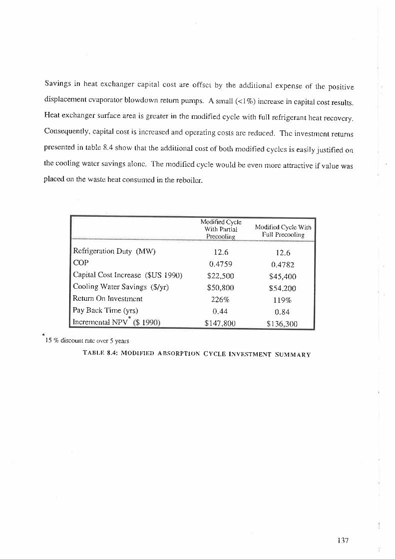
Savings in heat exchanger capital cost are offset by the adclitional expense of the positive
displacement evaporator blowdown return pumps. A small (<lVo) increase in capital cost results.
Heat exchanger surface area is greater in the modified cycle with full refrigerant heat recovery.
Consequently, capital cost is increased and operating costs are reduced. The investment returns
presented in table 8.4 show that the additional cost of both modified cycles is easily justified on
the cooling water savings alone. The modified cycle would be even ¡nore attractive if value was
placed on the waste heat consumed in the reboiler.
Modified CycleWith Partial
lng
Modified Cycle WithFull Precooling
Refrigeration Duty (MUD
COP
Capital Cost Increase ($US 1990)
Cooling Water Savings ($/yr)
Return On Investment
Pay Back Time (y*rs)
Incremental NPV 1
12.6
0.4759
$22,500
$50,800
226Vo
0.44
$147,900
12.6
0,4782
$45,400
$54,200
IL9Vo
0.84
$13 300
15 7o discount rate over 5 years
TABLE 8.4: MODIFIED ABSORPTION CYCLE INVESTMBNT SUMMARY
137

Foreach of the five aqua-ammonia absorption refrigeration cycles (figures 2'1 and 8'1 to 8'4)'
the minimum total cost of the requíred heat exchangers was determined ovef a range of evaporator
temperatures between 4oc and -12"C. These results are plotted in figure 8.7. The corresponding
coefficienS of performance obtained in these simulations are presented in frgure 8'8 as a function
of evaporator temPerature.
The capitar cost of the heat exchangers in the modified cycle without refrigerant heat recovery was
approximate ly 2.7Vo less than that of the equivalent conventional cycle' Also, the performance of
the modified cycle was approximately 5Vo greatet than the performance of the conventional cycle'
The total capital cost of the heat exchangers in the rnoclified cycle with partial refrigerant pre-
cooring was higher than that in the modified cycle without refrigerant pre-cooling due to the
increased number of heat exchange units. However, the heat exchange surface area was reduced
in this design. In larger refrigeration units, where the fixed charge on each heat exchanger is
small compared to the variable charge for increasing heat exchange surface area' the modified
cycle with partial refrigerant precooling may be less expensive than the cycle without refrigerant
heat recovery
For the given cost objective function, the cycles with full refrigerant precooling were less
attractive due to poor heat transfer and increased pressure drop in the refrigerant vapour
superheater.
within the expected error of these simulations, the coeff,rcients of performance (coP's) obtained
for each of the three cycles with refrigerant pre-cooling were icrenticar. The similarity between the
two modified cycres with refrigerant pre-cooling can be explained by the size of the refrigerant
vapour superheater. when optimised, this heat exchanger becomes very small' Hence' the
modified cycle with fuil precooring is essentiaily the same as the cycre with partial precooling.
The similarity with the conventional cycle with full precooling appears to be fortuitous'
138

Øtt
Oq)è¡6(.)Xt¡l
1 80000
1 60000
200000
1 40000
1 20000
1 00000
0.55
0.5
0.4
0.3 5
0.3
Convcntiorral. NoRefri gcran t Precooli n g
Conventional, FullRe lri geran t Precool i n g
-B -4 0
Evaporator Temperature ("C)
Modificd. NoRcfri gcrant prccooling
-------<>- Modif red. partiaÌ
Refrigerant heccoling
------rl- Modifi ed, FullRefrigerant precool ing
-16 -12
FIGURE 8.7: COMPARTSON OF CONVENTIONAL AND MODIFIED CYCLE
HEAT EXCHANCER COSTS
I4
Modified. NoRelrigerant Precooling
-=a- Modifìed. parriat
Refrigerant Preccol ing
-------l- Conventional. NoRefrigerant precoolin g
Convenûonal, FullRelrigerant Precool i ng(u
Ic€
-oqJ
O.
o
.9IEq)o()
0.45-{-
Modifìed, FullRefrigerant Precooling
-12 -B -4 0
Evaporator Temperature ('C)
FIGURE 8.8: COMPARISON OF CONVEN'IIONAL ^ND
MODIFIIID CYCLE
TIIIìRMODYNAMIC PTìRFO RMANCE
B4-16
139

On average, the coefficient of perfon'rrance of the cycles with refrigerant precooling were a furtJrer
g.3lo f,reater than the coefficients of performance obtained for the rnodified cycle without
refrigerant precooling.
To investigate the effect of constraints placed on the available heat source, the simulations were
repeated with the generator temperature held constant at 120oC. Under these conditions, the
influence of evaporator temperature on the minimum heat exchanger cost is presented in hgure
8.9.
The capital cost of the required heat exchangers in the modified cycle was less than that required
for the equivalent conventional cycle. Indeed, as the evaporator temperature approached the
lower feasible operating limit" the difference between the cost and performance of the two cycles
increased. At an evaporator temperature of -i2oC the cost of the heat exchangers for the
modified cycle was lTVo below that of the equivalent conventional cycle'
700000
500000
600000
400000
200000
1 00000
Convenúonal. NoRefrigerant Precooling
Conventional, FullRefrigerant Precooli ng
-.'- Modif red, No
Refrigerant Precooling
Modified, Partial
Relrigerant Preccoling
Modifled, FullRefngcrant Prccooling
300000
ecn
oOq)èo
dIxt¡
0
-16 -12 -B -4 0
Evaporator Tempcrature ('C)
T.'IGURE 8.9: COMI'ARISON OF CONVENI'IONAL AND MODtFf ED CYCLE
HE^T EXCHANGER COSTS WITIT GDNER^1'OR -I'IiMI'tìRATURI']' F-IXDD AT 120"C
Õ4
140

The condenser / evaporator cornbination in the rnoclified cycle may be viewed as a parrial
condenser for the distillation column. If this were the case, the improvement in perforrnance
obtained from the modified cycle could reflect the influence of placing an extra stage in the
distillation column only.
To investigate this hypothesis, a number of simulations of the modified and conventional cycles
were conducted to investigate the influence of increasing the number of theoretical stages in the
distillation column on cost and thermodynamic performance. The results of these simulations are
presented in Figure 8.10. The curves presented in figure 8.10 are not smooth because the feecl
location must be an integral number of plates from the top of the column.
In all cases, the capital cost of the heat exchangers in the modified cycle was lower than that
obtained from the conventional cycle. Clearly, figure 8.10 demonsffates that the improvement in
performance obtained from the modified cycle cannot be represented solely by the addition of an
extra theoretical plate to the distillation column.
1 85000---l- Convenrional, No Refrigemnr
Precooling
Modifi ed, No RefrigeranrPrecmling
1 750004
Number of Theoretical Trays
F-IGURE 8.10: INFLUENCE OF INCREASING 'rllD NUMBER OF THI.IORETICAL TRAYS
ON CONVT]NI'IONAI. AND MODIFIED CYCI,¡' IIIìAT EXCHANGIìR C^PfTAL COST
ØthoO0.)èo
aXr¡
1 83000
1 81 000
1 79000
1 77 000
5 q6 B7
141

The perfomrance of the conventional aqua-arÌlnlonia absorption refrigeration cycle is rnaximised
when the refrigerant purity is very high (approx. 99.9wt% NH3) ancl clrops off as refrigerant
purity decreases. Simulations were conducted to investigate the sensitivity of the conventional
and modified cycles, without refrigerant pre-cooling, to changing refrigerant purity. [n these
simulations, refrigerant purity was varied by changing the column pressure at a constånt
condenser temperatue. The results of these simulations a¡e illustrated in figure 8.1 1.
Figgure 8.1 1 shows that high purity ammonia refrigerant is required for optimum performance of
the modified aqua-ammonia absorption refrigeration cycle. However, the decrease in
performance due to increasing water contamination is not as dramatic as that seen in the
conventional cycle. This results in a more robust cycle which is more resilient to column foaming
or entrarnment.
0.9 8
0.9 6
0.94
0.9 2 Modified. No Refri gemnrPrecmling
0.9 Conventional. No RefrigcmntPrecooling
O.BB
98.5
1
q)Ic!
¡r
q)ÈqJ
clq)ú
9 9 99.5
Refrigerant Composition (mol 7o)
FIGURE 8.II: TNFLUENCE OF RET.RIGERAN'T COMPOSITION ON
CONVENTTONAI, AND MODIFITìD CYCLE PERFORMANCTì.
100
142

8.5 Discussion
On inspection, the proposed absorption refrigeration cycle with evaporator blowdown recycle is
very similar to the conventional cycle. However, significant improvements to cycle performance
are obtained with negligible increase in capital cost. The following discussion details the reasons
for the improved performance obtained from the modified cycle.
8.5.1 Absorbent Flowrate
The reduced circulation rate of absorbent required in the modified cycle is the principal reason for
improved perfonnance compared with the conventional cycle.
In order to maintain optimum reflux to the distillation column, a much larger fraction of
refrigerant entering the evaporator is returned to the distillation column. Consequently, the
composition of the liquid blowdown from the evaporator is richer in refrigerant and, for a given
evaporator temperature, the resulting evaporator pressure must be higher. This, in turn, leads to
increased pressure in the absorber so that less absorbent is required to dissolve the refrigerant
vapour exiting the evaporator.
In conventional designs, the evaporator blowdown is considerably richer in ammonia than the
strong absorbent exiting the absorber. (This fact can be deduced by comparing the compositions
of saturated liquid mixtures at the temperature of the evaporator and of the absorber).
Consequently, additional absorbent is required to dissolve the liquid blowdown stream. By
eliminating the practice of "dumping" liquid from the evaporator to the absorber, further
reductions in absorbent flowrate can be achieved.
The reduction in required absorbent circulation rate in the modified cycle leads to reduced losses
in the heat recovery exchanger and reduced sensible heating losses in the distillation column.
t43

8.5.2 Exergy Losses
Major sources of losses in absorption refrigeration machines result from the following;
(i) The mixing of streams with different composition.
(ii) Flashing of refrigerant across the expansion valve.
(iii) Indirect heat transfer with f,rnite thermal driving force.
In particular, losses occur in the conventional absorber due to mixing of the evaporator
blowdown (approx 94 mol%o ammonia) with absorption fluid (approx 36.1 mol%o ammonia after
refrigerant vapour has been absorbed). In the modified cycle, the evaporator blowdown is fed to
the top of the distillation column where the concentration of ammonia in the fluid is similar to that
of the evaporator blowdown liquid. Consequently, mixing losses are reduced.
Further reductions in cycle losses result from the lower flowrate of absorbent in the modified
cycle. This leads to reduced losses in the heat recovery heat exchangers, distillation column and
absorber.
An exergy analysis was conducted on both the conventional and modified cycles to further
determine the source of the reduced losses observed in the modified absorption refrigeration
cycle. The analysis was based on stream availabilities calculated by the PROCESS simulation
package using the equation of state proposed by Ziegler and Trepp (1984). The results of this
analysis are presented in table 8.5 for a 0.76MW refrigerator. Availability losses calculated by
Briggs (1971) are also presented in table 8.5 for comparison.
r44

Availability losses calculated in this study compare reasonably well with those presented by
Briggs, with the exception of the absorber and the heat recovery exchanger. [n this study, there
is a nett gain of work in the absorber. This is due to the 15oC reference temperature employed in
this study and the use of cooling water entering at27"C as the heat sink. Briggs assumed that
heat was rejected from the absorber to the heat sink at the reference temperature. Small losses
obtained by Briggs in the heat recovery exchanger reflect the close approach temperature (1.1 K)
assumed. In this study, the optimal approach temperature was calculated to be 8.8 K.
TABLE 8.5: COMPARISON OF CYCLE EXERGY LOSSES
Detailed examination of this table does not highlight any dramatic savings of work. The
reduction in losses obtained in the rnodihed cycle evaporator are prirnarily due to the refrigerant
precooler. Srnall reductions in losses associated with the heat recovery exchanger and the
distillation column, are due to the reduced circulation rate of absorbent as discussed above.
Conventional Cycle(Briees, l91I) Conventional Cycle
Modified Cycle withPa-rtial Pre-cooling
Evaporator
Refrigerarìt pre-cooler
Absorber recirc. pump
Refrigerant recirc. pump
Absorber
Evap Blowdown Absorption
Heat recovery exchanger
Distillation column
36.8 kW3.1
5.8
53.3 kW 48.4 kW
3.9
4.5
0.37
-60.6169.0
4.2
0.05
-s5.92.0
62.6
319.8
t2.6230.8
60.7
3t2.7
t45
Chapter 9
CONCLUSIONS
Background
Recent papers (Briggs, 1971 and Karakas,1990) have shown that the majority of losses in the
conventional absorption refrigeration cycle are confined to the absorber and the generator.
Dalichaouch (1990) also showed that, over a wide range of conditions, the performance of the
conventional absorption refrigeration cycle is less than thirty percent of the performance
predicted by the ideal second law.
Clearly, there is significant room for improvement in cycle petfonnance. Bearing this in mind,
investigations were conducted on a novel absorption refrigeration cycle which employs a liquid
- liquid separation step to separate the absorbent from the refrigerant. The cycle was chosen for
further examination with the intention of demonstrating the feasibility of eliminating the
distillation column generator in an absorption cycle heat pump. This could lower capital costs
and reduce one of the major sources of exergy losses.
The Thermodynamics of Working Fluid Mixtures
In addition to those cha¡acteristics which are desirable for absorbent - refrigerant pairs in the
conventional absorption refrigeration cycle, suitable absorbent - refrigerant pairs for the novel
cycle must exhibit "lower critical solution temperature behaviour" when mixed. Consequently,
a number of low molecula¡ weight tertiary amine - water pairs were selected as suitable
candidate pairs for application in the novel absorption refrigeration cycle.
To simulate the performance of the novel cycle, an accurate thermoclynamic model was required
to predict mixture phase equilibria at all points in the cycle. A five parameter NRTL model was
developed for this purpose. For each refrigerant - absorbent pair, the five parameters were
obtained by fitting the model to experimental vapour - liquid equilibriurn data by least squares
regression.
r46

Subsequent sir¡ulations of cycle performance ernployed a "black box" separator for the liquid
phase separation step, because no thermodynamic model was found capable of accurately
simulating the combined temperature dependent vapour - liquid and liquid - liquid phase
equilibria.
Experimental Results
Unfortunately, not all of the required experimental clata was available for the selected absorbent
- refrigerant pairs. Consequently, experimental vapour - liquid and liquid - liquid equilibrium
studies were conducted on dimethylethylamine - water and trimethylamine - water mixtures.
Liquid phase immiscibility had not previously been reported for either of these mixtures.
In this study, liquid phase separation was achieved for mixtures of dimethylethylamine and
water at temperatures above 99'C and at concentrations between 5 moI%o and37 mo|Vo amine.
Liquid phase separation was not observed for mixtures of trimethylamine and water at
temperatures up to 160"C. However, with the addition of 3 wt%o sodium chloride, liquid phase
separation was achieved at temperatures above 130'C. Unfortunately, significant uncertainty is
associated with the liquid phase co-existence curve obtained for mixtures of trimethylamine,
water and salt. This uncertainty results, primarily, from the high pressure and consequently
high evaporation losses inside the sample ampoules at experimental conditions.
Vapour - liquid equilibrium data was obtained in a static equilibrium apparatus for
dimethylethylamine - water and trimethylarnine - water mixtures between 10'C and 50oC.
Vapour pressure data was obtained over the entire concentration range for mixtures of
dimethylethylarnine and water. Unfortunately, vapour pressure clata could only be obtainecl
over a limited concentration range at ternperatures above 20oC for mixtures of trimethylamine
and water. For high concentrations of trimethylarnine, the vapour pressure was too high to be
measured on tlìe ñìercury lnanometer.
147

The Novel Absorption Refrigeration Cycle
The basic novel absorption cycle heat purnp was simulated on a computer using the
PROCESSTM chemical plant simulation software package. Results of these simulations, using
diethylmethylamine and water as the refrigerant - absorbent pair, showed that refrigeration
could only be obtained over a limited range of temperatures. Perfoffn¿mce fell dramatically with
decreasing evaporator temperature. The performance of the cycle with dimethylethylamine and
water as the working fluid pair was worse because of the higher water (absorbent) content in
the refrigerant,
Thermodynamic analysis of the cycle demonstrated that the boiling point elevation between the
refrigerant and the absorbent must be zeÍo at the high pressures required in the liquid phase
separation drum. Clearly, the rate of change in this boiling point elevation, with decreasing
pressure, is insufficient to obtain a reasonable boiling point elevation between the evaporator
and the absorber in the novel absorption refrigeration cycle.
Unfortunately, there ¿ue very few alternative mixtures which exhibit the required liquid - phase
behaviour. For these reasons, the novel absorption refrigeration cycle is unlikely to find
commercial application. However, the feasibility of the novel cycle was successfully
demonstrated. This result conhrms that it is possible to elirninate the necessity for refrigerant
vaporisation in the generator ancl, consequently, it is possible to replace the distillation column
with a more thennodynarnically efficient unit operation.
The Novel Absorption Refrigeration Cycle With Distillation
The potential of a number of cycles containing both the liquid phase separation step and the
distillation step for recovering refrigerant, was also investigatecl. The performance of these
"hybrid" cycles were simulated using PROCESSTM to detennine the optimum cycle
configuration. Dimethylethylamine and water were used as the working fluids in these
simulations because the nonnal boiling point of dimethylethylamine is significantly lower than
that of diethylmethylarnine.
148

One of the cycles developecl ernployed the additional distillation step to further purify the
absorbent stream after initial refrigerant recovery was achieved in the liquid phase separation
drum. Due to the significant level of absorbent contamination in the refrigerant stream, the
concept of returning the evaporator blowdown to the generator (initially applied to the basic
novel absorption cycle only) was employed in this cycle. In this case, the evaporator
blowdown recycle stream was employed as reflux to the clistillation column. This concept was
subsequently applied to the conventional aqua - ammonia absorption refrigeration cycle with
encouraging results.
Despite this advance, the performance of each of the novel absorption refrigeration cycles
including the additional distillation step was worse than the perfonnance of the conventional
absorption refrigeration cycle employing the same working fluids. Surprisingly, the novel
cycle with the best thermodynamic performance employed the distillation column to rectify the
refrigelant phase exiting the liquicl phase separation drum. In this cycle, all of the fresh
refrigerant must be evaporated and condensed prior to entering the evaporator at low pressure,
which defeats the initial purpose of investigating cycles which employ the liquid phase
separation step.
Simplified Analysis for Cycles With Trimethylamine and Water
Due to the poor experimental results obtained for mixtures of trimethylamine and water, the
potential of the novel absorption refrigeration cycles with trimethylamine as the refrigerant was
not examined in detail. Instead, the absorbent flowrate required to completely dissolve
refrigerant vapour of assumed concentration, was determined as a ratio of the refrigerant vapour
flowrate. By cornparison with the conventional amrnonia - water working fluid pair, the
trimethylamine - water working fluid pair was shown to have no commercial potential in any of
these absorption refrigeration cycles.
149

The Novel Absorption Cycle Heatpump
The previous cycles employed mixtures exliibiting lower critical solution telnperature behaviour
as working fluids in novel absorption refrigeration cycles. In a further developrnent of this
concept, a type II heat pump cycle was proposed and developed. The cycle employs working
fluid mixtures exhibiting upper critical solution temperature behaviour. The cycle accepts heat
at some intermediate temperature level and rejects a portion of this heat at high temperature.
The performance of this cycle was simulated on the PROCESSTM chemical plant simulation
package using cyclohexane and aniline as the working fluids. This working fluid pair was
considered ideal as a very large boiling point difference exists between the two compounds and
liquid phase separation occurs over a large concentration range at ambient temperature.
Results of these simulations showed that the boiling point elevation which could be achieved
between the evaporator and the absorber, with these working fluids, was less than 10 K.
Performance w,as also shown to fall dramatically with increasing absorber temperature. Poor
performance was attributed to the high absorbent ci¡culation rate requirecl.
A number of alternative heat pump cycles including the liquid phase separation step and an
additional distillation step were also investigated. Unfortunately, the rate of decrease in the
bubble point temperature for mixtures of cyclohexane and aniline is very low at cyclohexane
concentrations between 307o and 100Vo. Consequently, the aclclition of volatile working fluid
phase rectification or absorbent phase stripping steps does not signihcantly increase the boiling
point elevation which can be achieved between the evaporator and the absorber.
lncreased boiling point elevations were achieved, however, when the liquid phase separation
step was applied to the evaporator blowclown stream. Unfortunately, the small size of this
strearn, the complex heat recovery network requirecl and the low refrigerant purity required to
make this cycle feasible resultecl in poor thennoclynarnic performance compa,red to that obtained
in the conventional type II heat pump employing the same working fluicl pair.
150

The Modified Aqua - Ammonia Absorption Refrigeration Cycle
While the feasibility of each of the cycles discussed above was demonstrated, commercial
application of these cycles is unlikely due to the low boiling point elevations achieved and the
poor cycle thermodynamic perforrnance.
However, these simulations successfully highlighted the potential of recycling the evaporator
blowdown in order to supply reflux to the rectification section of the conventional absorption
cycle distillation column. This modification to the conventional cycle was simulated on
PROCESSru using the thermodynamic model proposed by Ziegler and Trepp (1984) for
predicting the phase behaviour of ammonia - water mixtures.
Over a wide range of conditions, these simulations indicate a reduction in total heat exchange
surface area and an increase in thermodynamic performance of approximately ltve percent (57o)
when the modified cycle is compared with the conventional aqua - ammonia absorption
refrigeration cycle.
As a much larger fraction of refrigerant entering the evaporator is returned to the distillation
column in the rnodified absorption refrigeration cycle, the cornposition of the liquid blowdown
from the evaporator is richer in refrigerant. Thus, for a given evaporator temperature, the
resulting evaporator/ absorber pressure must be higher so that absorbent circulation rates can be
reduced. This is the primary reason for the improved performance of the modified cycle.
151

Recommendations
The results of this study indicate that the conventional absorption cycle heat pump distillation
column generator can be replaced by alternative separation techniques. However, the
alternative separation technique of liquid phase sepa-ration explored in this thesis, did not prove
attractive when compared with the conventional cycle. Consequently, further examination of
liquid phase separation in an absorption cycle heat pump should be abandoned. Other
separation techniques such as fractional crystallisation or membrane filtration are worthy of
further investigation.
An interesting modif,rcation to the conventional absorption refrigeration cycle, arising from this
work, was the application of evaporator blowdown recycle to provide reflux to the rectification
section of the conventional distillation column. This modification was shown to provide
efhciency improvements with a nett reduction in heat transfer surface area. Consequently, pilot
scale demonstration of this cycle is recommended.
152

Appendix A
EXPERIMENTAL DATA
rT P mmHg
5.54
10.31
14.92
14.97
19.56
24.51
26.44
3r.36
31.90
34.69
38.87
41,.51
44.85
48.41
228.88
282.02
338.79
342.59
409.27
492.89
s32.39
632.s6
646.81
71.4.29
825.51
903.70
1005.52
t126.t2
TABLE 4.1: VAPOUR PRESSURE DATA FOR DIMETHYLETHYLAMINE
153

T oC Xdmea P mmHg T oC Xd.nea P rnmHg ToC Xdmea P mmHg
10.01 0.jr't4
0.0618
0.1656
0.2533
0.338s
0.4885
0.6071
0;7363
0.8081
0.8719
32.04
87.58
123.14
155.57
186.87
233.3
242.54
255.42
260.22
261.12
6l.85
150.6 r
200.63
244.86
283.37
331.65
358.00
314.41
384.s0
39r.35
119.56
254.48
3r4.76
313.56
423.22
487.48
515.53
541.89
s60.00
5æ.29
19.53 0.0174
0.0618
0.1656
0.2533
0.3385
0.4885
0.6011
0.7363
0.8081
0.8719
29.11 0.0r't4
0.0618
0.1656
0.2533
0.338s
0.4885
0.6017
0.7363
0.8081
0.8719
T"C Xdmea P mmHg T "C Xdmea P mmHg
38.91 0.0174
0.0618
0.1656
0.2533
0.338s
0.488s
0.6011
0.1363
0.8081
0.8719
219.t6
409.08
490.60
560.93
618.91
699.16
135.28
142.14
78-5.45
198.M
48.59 0.0r74
0.0618
0.1656
0.2533
0.3385
0.4885
0.6077
0.1363
0.8081
0.8719
366.38
629.69
135.90
815.21
881.24
912.09
toLz.42
1053.86
1083.29
1096.40
TABLB 4.2: VAPOUR - LIQUID EQUILIBRIUM DATA FOR
DIMETHYLETHYLAMINE - WATER MIXTURES
t54

T qC Xfitru P mmHg T'C Xtna P mmHg T cC Xuna P mmHg
10.66 0.0034
0.0336
0.0614
0.0803
0.1630
0.2062
0.3127
0.5305
0.5639
0.63s8
0.6480
0.6483
0.8320
0.8593
0.9142
0.9133
32.04
75.05
t43.21
168.50
382.83
396.34
540.49
736.80
76r.29
831.22
810.73
855.00
907.05
890.19
923.23
9s6.48
19.88 0.0034
0.0336
0.0614
0.0803
0. l 630
0.2062
0.3121
0.5305
0.5639
0.6358
0.6480
0.6483
0.8320
0.8s93
0.9142
0.9733
34.1 8
133.89
236.34
216.08
562.15
577.67
164.71
1031.33
1052.r3
1120.92
1119.45
1r69.88
1253.4
1234.t3
1289.56
1322.6r
t373.90
t466.60
24.43 0.6483
0.8320
T rc Xftra P mmHg T'C Xûtra P mmHg Trc Xmua PmmHg
29.60 0.0034
0.0336
0.0614
0.0803
0.1630
0.2062
0.3r27
0.530s
0.5639
0.63s8
0.6480
60.89
224.10
378.96
444.31
8tt.92
841.21
1080.63
r4r3.6l
1438.t7
t52r.9t
t520.94
t03.62
342.98
569.37
682.41
1135.33
48.85 0.0034
0.0336
0.0614
0.0803
t68.21
489.52
818.25
1013.08
39.28 0.0034
0.0336
0.0614
0.0803
0.1630
TABLE 4.3: V^POUR - LIQUID EQUILIBRIUM DATA FOR
TRIMETHYLAMINE - WATER MIXTURES
155

AmineComposition Temperature
("c)lm ol"/"
6.0
8.1
13.7
20.7
26.8
29.4
37.7
102.4
100.2
9 9.6
9 8.8
99.1
9 9.3
100.3
TABLE 4.4: LIQUID - LIQUID EQUILIBRIUM DATA FOR
DIIMETHYLETHYLAMINE . WATER MIXTURES
AmineComposition
(m o l%)
Temperature
("c)
11.8
13.8
14.8
1 6.0
1 8.6
1 9.6
23.0
26.5
144.3
1 35.6
1 36.3
130.9
131.9
130.2
123.6
120 .4
TABLE A.5: LIQUID - LTQUID EQUILTBRIUM DATA F.OR
TRIMETHYLAMINE - 37o NaCl SOLUTION MIXTURES
156

Appendix BNRTL PARAMBTBR DBTBRMINATION FROM VAPOUR .
LIQUID EQUILIBRIUM DATA
Program Description
A computer program was employed to generate values for the five parameters, required in the
NRTL model described in chapter 4, which give the best fit to the experimental data. The
program employs the Powell algorithm to minimise the objective function. The objective
function was defined as the sum of the squared error between each of the experimental data
points and that predicted by the thermodynamic model with the selected five parameters (chapter
4 equation 4.6)
The five adjustable parameters àt, à2, b' b, and û,, in the NRTL model, were obtained using a
two stage minimisation procedure. This procedure is illustrated in the block diagram presented
in figure 8.1. For given values of b, and b' the error function was minimised by manipulation
of a' q and ü. New values for b, and b, were chosen, and optimum values for a,, a, and cx,
recalculated. The process continued until no further reduction in the error could be achieved. A
listing of the fortran computer program is presented below. The subroutines POWELL,
LINMIN, MNBRAK, BRENT and F1DIM employed in this procedure, were obtained from
Press et. al. (1989) with minor modifications. The reader is refered ro rhis text for further
information on these programs.
This two stage approach was chosen for its robustness. Attempts to minimise the error
function with a single stage Powell algorithm gave varying results depending on rhe initial
values chosen for a,, %, b' b, and a.
t5l

1. Select initial values for a,, àr,b, br, o and two search
vectors
2. Calculate new a,, a, and a to give the initial minimum
error for and
3. Sea¡ch along the fi¡st vector to determine the upper and
lower bounds (around the minimum) for b, and br.
4. Using the first vector, shrink the upper and lower bounds
for b, and br.until the minimum error is achieved.
5. Sea¡ch along the second vector to determine the upper and
lower bounds (around the minimum) for b, and br.
6. Using the second vector, shrink the upper and lower
bounds for b, and b,until the rninimurr error is achieved.
7. Replace the vector which achieved the largest error
reduction with a new vector equal to the change in b, and b,
achieved in the previous two line searches.
8. Repeat procedures 3 tol until no further improvernent is
made to b, and br.
FIGURE ß.1: LocIC FOR FINDING V/tLUlìs F-Oll THE MODDL P^RAìvlETIìRS GIVING THE
MINIMUM LEAST SQUARE ERROR
158

Program Listinqs
program nrtlT
This program runs the outer minimisation loop for detennining the best fit values for bl andb2
dimen sion xxp(20,20),pp (20)
coÍrnon /par/e,f,g
daø nl 2 / np /2 / f toU 0 .00 I /open(unit=4,status='old')
read(4,11) e Reading in initial values for al,a2,alpha
read(4,11) fread(4,11) g
close(unit=4)
clo i=l,n Reading in initial values for b1,b2 and assigning initial search vectors
read(44,11)pp(i)
xxP(i,i)=1.Q
end do
11 format(f8.4)
callpowell2(pp,xxp,n,np,ftol,iter,fret) Callingthepowellsubroutinetoconduct
the error minimisation sea¡ch
do i=l,4write(9,20)i,pp(i)
end do
20 format (' a',i2,' =',fl 0.5)
end
function func2(pp)
This function calculates the error between the exper-irnentål data and the correlation for the given
correlation parameters.
dimension pp(7)
comrnon /terrí a,b
a=pp(1)
b=pp(2)
call nrtl(en) Calling the subroutine NRTL to determine the optirnum values
of ay, a2, and c¡ for the selected b1 and b2
write(6,12)err,a,b
12 format(' error=',f9.3,x,f10.6,x,fl0.6)
159

func2=err
retum
end
subroutine nrtl(fret)This subroutine returns the minimum error between the experimental data and the NRTL
equation which can be obtained by manipulating aL, az and cr for given values of b1 and b2.
This is the inner minimisation loop
dimen sion xxp (20,20),p (20 )
coffrmon lpail e,f,g
datz nl 3 I np ß I f toV 0.00 I I
P(1)=e
P(2)=fp(3)=g
call powell(p,xxp,n,np,ftol,iter,fret) attl"T the POWELL subroutine to conduct the
mrnrmrsatron
do i=1,n
write(9,20)i,p(i)
end do
20 format(' a',i2,' =',fI2.5)return
end
function func(p)
dimension p(7)
common /tem/ tal,ø2
open (unit= I 4,statu s='old')
read(14,1000)nvl
1000 format(i2)
err=0.0
do i=1,nvl
read(14,1000)np
read(14,82)tvl
tet=tvl+Z13.14
Reading the nurnber of isothennal V-L data sets
Reading the number of data points in the i'th V-L data set
Reacling the temperature of the i'th V-L data set
160

¡12:(p(1)+tal*tet-2.58-8*tet**4)11.981211(tvl+273.14) CalculatingNRTLparameters
¡)l =(p (2) +ta2* tet) / I .9 87 2 I / (wt+27 3 . I 4)
alpha=p(3)
gl2-.=exp (- alp h a * t 1 2)
921=exp(alpha*t21)pvap 1=10* *(1 .55466-1002.17Il(tvl+247.8 85)) Calculating pure component
pvap2=10**(8.07131-1730.63/(Nl+233.426)) vapour pressures
do j=1'nO
read(14,83)pres,xl
vl I n y 1 =( 1 - xl)* * 2* (t2 I x (g2 I I (xl+( 1 - xl) * 92 I ) ) * * 2
xc -.'utl2* 912/(l-xl+xl*g12)**2)y1=exp(vllnyl) Calculating the component 1 activity coefficients
ypl=xlxyl*pvapl and partial pressures at data point jvllny2=xlx * 2* (tlL* (g1 2/( 1 -xl+xl * gI2))* *2
* lur2l*g2ll(xl+(l-xl)*g2I)**2)y2=exp(vllny2)
yp2=(1-xl)*y2*pvap2
err=err*(pres-yp1-yp2)**2/pres*x2 calculating the normalised error between
end do experiment and model
end do
82 format(f8.4)
83 format(f8.2,f8.5)
func=err
close(unit=14)
retum
end
S UB RO UTINE PO WELL2( p p,xxn,N,NP, FTO L,ITER,FR ET)
Minimisation of a function FUNC2 of N variables. (FUNC2 is not an a.rgument, it is a fixed
function narne) Input consists of an initial starting point PP that is a vector of length N; an
initial matrix XXN whose logical dimensions a¡e N by N, physical dimensions NP by NP, and
whose colu¡nns contain the initial set of directions (usually the N unit vectors); and FTOL, the
fractionaì tolerance in the function value such that failure to decrease by more than this amount
on one iteration signals doneness. On output, PP is set to the best point found, XI is the then -
current direction set, FRET is the returned function value at PP, and ITER is the number of
iterations taken. The routine LINMIN2 is usecl
161

PARA METER (NMAX=20,ITMAX=200)
DIMENS ION pp (6),xxn (6, 6),PT(NMAX),PTT(NM AX),x iT(NMAX)FRET=FUNC2(pp)
DO 11 J=1,N
PT(J)=pp(J)
11 CONTINUE
ITER=0
I ITER=ITER+1
FP=FRET
IBIG=0
DEL=0.
DO 13 I=1,N
DO 12 J=l,NXIT(J)=xxn(J,I)
12 CONTINUE
CALL LINMIN2(pp,XIT,N,FRET)
rF(AB S (FP-FRET).GT.DEL)THEN
DEL=ABSG'P-FRET)
IBIG=I
ENDIF
13 CONTINUE
IF(2. *AB S(FP-FRET). LE. F rOL* (ABS (FP)+ABS (FRET)))RETURN
IF(ITER.EQ.ITMAX) PAUSE'Powell exceeding maximum iterarions.'
DO 14 J=l,NPTT(J)=2. "pp(J)-PT(J)XIT(Ð=pp(J)-PT(J)
PT(J)=pp(J)
14 CONTINUE
FPTT=FUNC2(PTT)
rF(FPTT.GE.FP)GO TO 1
T=2.* (FP-z. *FRET+FPTT)*(FP-FRET-DEL)*x2-DEL*(FP-FPTT)i r.2
rF(T.GE.0.)GO TO 1
CALL LINMIN2 (pp,XIT,N,FRET)
DO 15 J=l,Nxxn(J,IBIG)=XIT(J)
15 CONTINUE
GOTO 1
END
t62


PTT(J)=2.*P(J)-PT(J) Save the old star-ting point
xIT(J)=P(J)-PT(J)
PT(J):P(J)
14 CONTINUE
FPTT=FUNC(PTT) Function value at the extrapolated point
IF(FPTT.GE.FP)GO TO 1 One reason not to use new clirection
1=2. * (FP-2. *FRET+FPTT)* (FP-FRET-DEL) x *2-OUt* (FP-FPTT) * *2
IF(T.G8.0.)GO TO 1 Other reason not to use new direction
CALL LINMIN(P,XIT,N,FRET) Move to the minimum of the new direction
DO 15 J=1,N And save the new direction
xxn(J,IBIG)=XIT(J)
15 CONTINUE
GO TO I Back for another iteration
END
S UB ROUTINE LINMIN2(p p,XI,N,FRET)
Given an N dimensional point pp and an N dimensional direction XI, this program moves and
resets pp to where the function FUNC(pp) takes on a minimum along the direction XI from pp.
The program also replaces XI by the actual vector displacernent that pp was moved. The value
of FUNC at the returned location P is returned as FRET. These tasks are accomplished by
calling the subroutines MNBRAK2 and BRENT2.
PARAMETER (NMAX=50,TOL:3. E-3)
EXTERNAL FlDIM2
DIMENSION pp(4),XI(N)
coMMoN ß rcoM2l NCOM,PCOM(NMAÐ,XICOM(NMAX)
NCOM=N
PCOM(J)=pp(J)
xICOM(J)=XI(J)
11 CONTINUE
AX:0.XX:1.BX=2.
CALL MNBRAK2(AX,XX,BX,FA,FX,FB,F1 DIM2)
FRET=BRENT2(AX,XX,BX,F 1 DIM2,TOL,XMIN)
DO 12 J=1,N
164

XI(J)=¡¡4IN*XI(J)pp(Ð=pp(J)+Xr(J)
12 CONTINUE
RETURN
END
SUBROUTINE LINMIN(P,XI,N,FRET)Given an N dimensional point P and an N dimensional direction XI, this program moves and
resets P to where the function FUNC(P) takes on a rninimurn along the direction XI from P.
The program also replaces XI by the actual vector displacement that P was moved. The value
of FUNC at the returned location P is returned as FRET. These tasks are accomplished by
calling the subroutines MNBRAK and BRENT.
PARAMETER (NMAX=5 0,TOL=3. E-3)
EXTERNAL F1DIM
DTMENSTON P(r9,XI(r9
coMMoN iF 1 COW NCOM,PCOM(NMAX),XrCOM (NMAX)
NCOM=N set up common block
DO 11J=l,NPCOM(J)=P(J)
xICOM(J)=XI(J)
11 CONTINUE
AX=0. Initial guess for brackets
XX=1.BX=2.
CALL MNBRAK(AX,XX,BX,FA,FX,FB,FlDIM)FRET=BRENT(AX,XX,BX,F 1 DIM,TOL,XM IN)
DO 12 J=l,N Constructing the vector results to return
XI(J)=¡¡4IN*XI(J)P(J)=P1¡¡*XI(J)
12 CONTINUE
RETURN
END
165

SUBROUTINE MNBRAK2(AX,BX,CX,FA,FB,FC,FUNC2)PARAMETER (GOLD=1.61 8034, GLIMIT:100., TINY=1.E-20)
FA=FUNC2(AX)
FB=FUNC2(BX)
rF(FB.GT.FA)THEN
DUM=AX
AX=BXBX=DUM
DUM:FBFB=FA
FA=DUM
ENDIF
CX=BX+GOLD*(BX-AX)
FC=FUNC2(CX)
1 rF(FB.GE.FC)THEN
R=(BX-AX)*(FB-FC)
Q=(BX_CX)*(FB_FA)
u=BX-((BX-CX¡ xq- (B X-AX) xR)/(2. *SrcN(MAX(AB S (Q_R),TrNy),Q_R))
ULIM=B X+GLIMIT* (CX-BX)
rF((B X-U) r. (U-CX). GT.0.)THEN
FU=FUNC2(U)
rF(FU.LT.FC)THEN
AX=BXFA=FB
BX=U
FB=FU
GOTO 1
ELSE IF(FU.GT.FB)THEN
CX=U
FC=FU
GOTO 1
ENDIF
U=CX+GOLDx(CX-BX)
FU=FUNC2(U)
ELSE IF((CX-U)*(U-ULrM).GT.0.)THEN
FU=FUNC2(U)
rF(FU.LT.FC)THEN
r66

BX=CX
CX=U
U=CX+GOLD*(CX-BX)
FB=FC
FC=FU
FU=FUNC2(U)
ENDIF
ELS E rF((U-ULrM) * (ULrM-CX).GE.0.)THEN
U=ULIM
FU=FUNC2(U)
ELSE
U=CX+GOLD*(CX-BX)
FU=FUNC2(U)
ENDIF
AX=BX
BX=CX
CX=U
FA=FB
FB=FC
FC=FU
GOTO 1
ENDIF
RETURN
END
S UBROUTINE MNBRA K(AX,B X,C X, FA,FB,FC,FUNC)
Given a function FUNC, and given distinct initial points AX and BX, this routine searches in
the downhill direction (defined by the function as evaluated at the initial points) and retums new
points AX, BX and CX which bracket a minimum of the function. Also returned a¡e the
function values at tl.ìe three points FA, FB and FC
PARAMETER (GOLD:1.6 18034, GLIMIT=100., TINY=I.E-20)
FA=FUNC(AX)
FB=FUNC(BX)
IF(FB.GT.FA)THEN Switch roles of A and B so that we can go downhill
DUM:AX in the direction frorn A to B
167
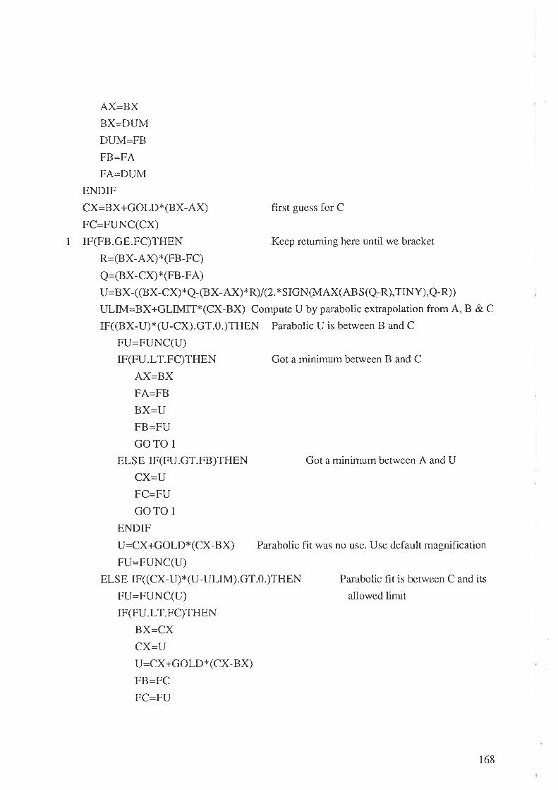
AX=BXBX=DUM
DUM=FB
FB=FA
FA=DUM
ENDIF
CX=BX+GOLD*(BX-AX) first guess for C
FC=FUNC(CX)
1 IF(FB.GE.FC)THEN Keep returning here until we bracket
R=(BX-AX)x(FB-FC)
Q=(BX-CX)*(FB-FA)u=BX- ((BX-CX¡ x q- @X-Rp xR)/(2. x SrcN(MAX(AB S (Q-R),TrNY),Q-R))
ULIM=BX+GLIMIT*(CX-BX) Compute U by parabolic extrapolation from A, B & C
IF((BX-U)*(U-CX).GT.O.)THEN Parabolic U is between B and C
FU:FUNC(U)IF(FU.LT.FC)THEN Got a minimum between B and C
AX=BXFA=FB
BX=U
FB=FU
GOTO 1
ELSE IF(FU.GT.FB)THEN Got a minimum between A and U
CX=U
FC=FU
GOTO 1
ENDIF
U=CX+GOLD*(CX-BX) Pa¡abolic fit was no use. Use default magnification
FU=FUNC(U)
ELSE IF((CX-U),'(U-ULIM).GT.0.)THEN Parabolic f,rt is between C and its
FU=FUNC(U) allowed limit
rF(FU.LT.FC)THEN
BX=CX
CX=U
U=CX+GOLD*(CX-BX)
FB=FC
FC=FU
168

FU:trUNC(U)ENDIF
ELSE IF((U-ULIM)*(ULIM-CX).GE.0.)THEN Limit parabolic U to max allowed
U=ULIMFU=FUNC(U)
ELSE Reject parabolic U. Use default magnification
U=CX+GOLD*(CX-BX)
FU:FUNC(U)ENDIF
AX=BX
BX=CX
CX=U
FA=FB
FB=FC
FC=FU
GOTO 1
ENDIF
RETURN
END
FUNCTION BRENT2(AX,BX,CX,F,TOL,XMIN)Given a function F, and given a bracketing triplet of abscissas AX, BX, CX (such that BX is
between AX and CX, and F(BX) is less than both F(AX) and F(CX)), this routine isolates the
minimum to a fractional precision of about TOL using Brent's method. The abscissa of the
minimum is returned as XMIN, and the minimum function value is returned as BRENT2,the
returned function value.
PARAMETER (ITMAX= 1 O0,CGOLD =. 3 8 19 660,ZEPS = 1 . 0 E- 1 0)
A=MIN(AX,CX)B=MAX(AX,CX)V=BX
W=V
X=VE=0.
FX=F(X)
FV=FX
r69

FW=FX
mm=1
m=1
DO 11 ITER=I,ITMAX
XM=0.5*(A+B)
TOLl=TOL*ABS(X)+ZEPS
TOL2=2.*TOLI
rF(AB S (X-XM). LE. CrOL2-.s *(B-A))) GOTO 3
if(m.eq.5) then As the program is so slow, the following code is
write(6,56) used to allow the user to make judicious decisions
56 format('are we close enough? !es=2 no=l') about whe¡r to finish minimising
read(5,57)mm
57 format(i2)
if(mm.eq.2) goto 3
m=1
end ifm=m*1
wrire(6,57)m
rF(ABS (E).GT.TOL1) THEN
R=(X_\{)*(FX_FV)
Q=(X_V)*(FX_FW)P=(X-V)*Q-(X-W;xp
Q=2.*(Q-R)IF(Q.GT.0.) P=-P
Q=ABS(Q)ETEMP=E
E=D
rF(AB S (P).G8. AB S (. 5 * Qx ETEM P). O R. P. LE. Q * (A -X). O R.
* P.GE.Q*@-X)) GOTO I
D=p/e
U:X+DIF(U-A.LT.TOLL .OR. B-U.LT.TOL2) D=SIGN(TOL I,XM-X)GOTO 2
ENDIF
I rF(X.GE.XM) THEN
E=A-X
t70

2
ELSE
E=B-X
ENDIF
D=CGOLDxE
rF(ABS (D).GE.TOL1 ) THEN
U=X+D
ELSE
U=X+SIGN(TOL1,D)
ENDIF
FU=F(U)
rF(FU.LE.FX) THEN
rF(u.GE.X) THEN
A=X
ELSE' B=X
ENDIF
V='W
Iry=Il\M
W=X
FW=FX
X=UFX=FU
ELSE
rF(u.LT.X) ]ïENA=U
ELSE
B=U
ENDIF
rF(FU.LE.FW .OR. W.EQ.X) THEN
V=W
FV=FW\ü=U
FW=FU
ELSE rF(FU.LE.FV .OR. V.EQ.X .OR. V.EQ.W) THEN
V=U
FV=FU
177

ENDIF
ENDIF
11 CONTINUE
write(6,38)
38 format('Brent2 exceed maxirnum iærations.')
3 XMIN=XBRENT2=FX
RETURN
END
FUNCTION B RBNT (AX,BX,CX,F,TO L,X MIN)Given a function F, and given a bracketing triplet of abscissas AX, BX, CX (such that BX is
between AX and CX, and F(BX) is less than both F(AX) and F(CX)), this routine isolates the
minimum to a fractional precision of about TOL using Brent's method. The abscissa of the
minimum is returned as XMIN, and the minimum function value is returned as BRENT, the
returned function value.
PARAMETER (ITMAX= 1 0O,CGOLD=. 3 8 1 9 660,ZEPS = 1. 0 E- 1 0)
A=MIN(AX,CX) A and B must be in ascending order, though the input abscissas
B=MAX(AX,CX) need not be
V=BX
W=V
X=V
E=0. This will be the distance moved on the step before last
FX=F(X)
FV=FX
FW=FX
DO 11ITER=I,ITMAX
XM=0.5x(A+B)
TOL1=TOL*ABS(Ð+ZEPS
TOL2=2.*TOLI
IF(ABS(X-XM).LE.(TOL2-.5*(B-A))) GOTO 3 Test for done here
IF(ABS(E).GT.TOLl) THEN Construct a trial parabolic ht
R=(X_g/)*(FX_FV)
Q=6_V)*(FX_FW)P=(X_V)*Q_fi_W¡*B
r72
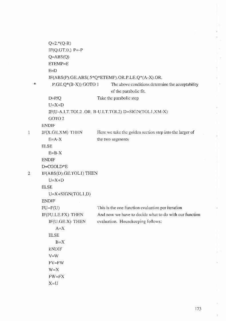
*
Q=2.*(Q-R)IF(Q.GT.O.) P=-P
Q=ABS(Q)
ETEMP=E
ÞDrF(AB S(p).GE. AB S (.5xQ*ETEMp). OR. p.LE. Q*(A-X). OR.
P.GE.Q*(B-X) GOTO 1 The above conditions determine the acceptability
of the parabolic fit.
D=P/Q Take the parabolic step
U=X+D
IF(U-A.LT.TOLL.OR. B-U.LT.TOL2) D=SIGN(TOL1,XM-X)
GOTO 2
ENDIF
IF(X.GE.XM) THEN Here we take the golclen section step into the larger of
E=A-X the two segments
ELSE
E=B-X
ENDIF
D=C]GOLD*E
rF(ABS (D).GE.TOL1) THEN
U=X+D
ELSE
U=X+SIGN(TOL1,D)
ENDIF
FU=F(U) This is the one function evaluation per iteration
IF(FU.LE.FX) THEN And now we have to decide what to do with our function
IF(U.GE.X) THEN evaluation. Housekeeping follows:
A=X
ELSE
B=X
ENDIF
V=W
FV=FW
W=X
FW=FX
X=U
1
2
t73
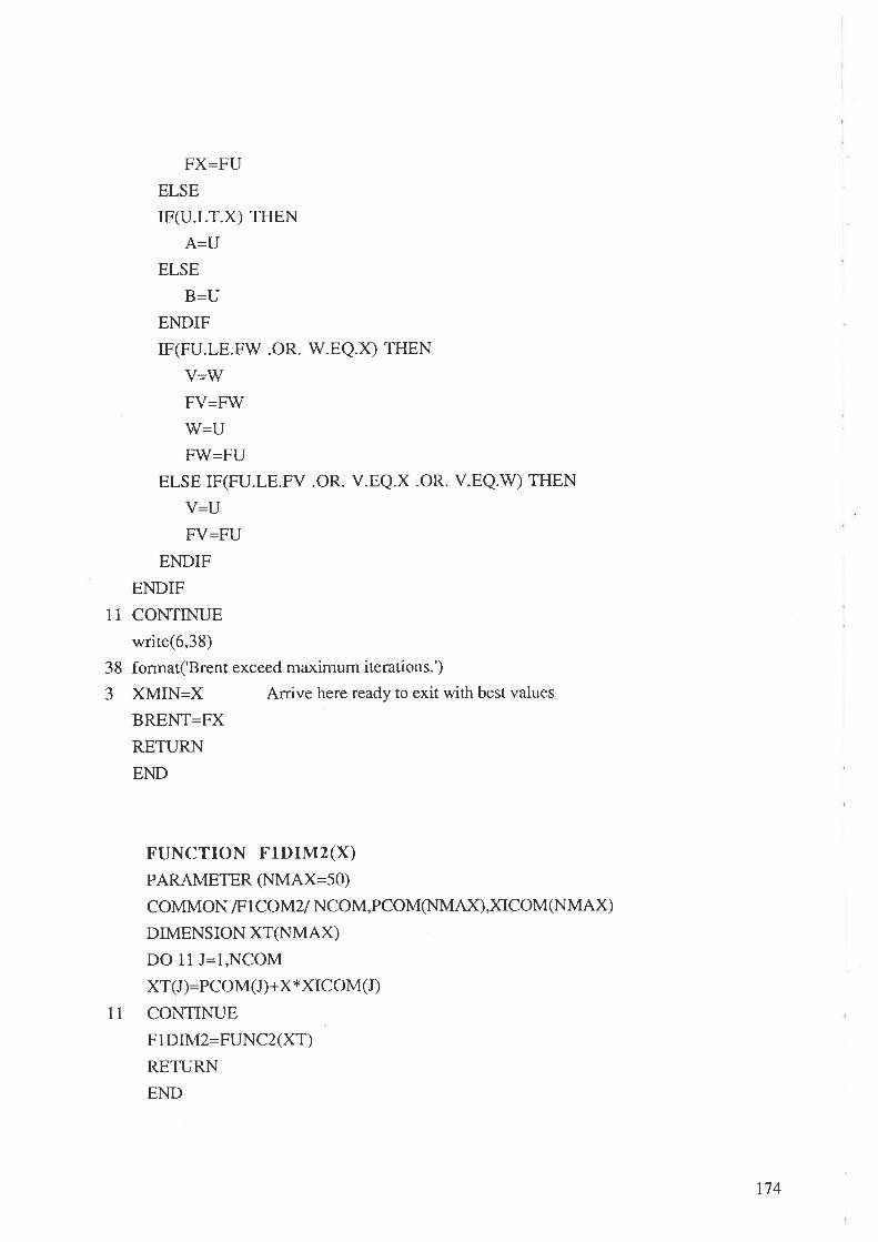
FX=FU
ELSE
rF(u.LT.X) THEN
A=U
ELSE
B=U
ENDIF
rF(FU.LE.FV/ .OR. V/.EQ.X) THEN
V=W
FV=FW'W=U
FW=FU
ELSE IF(FU.LE.FV .OR. V.EQ.X .OR. V.EQ.W) THEN
V=U
FV=FU
ENDIF
ENDIF
11 CONTINUE
write(6,38)
38 format('Brent exceed maximum iterations.')
3 XMIN=X Arrive here ready to exit with best values
BRENT=FX
RETURN
END
FUNCTTON F1DIM2(X)PARAMETER (NMAX=5O)
coMMoN ß LCOì/^Z/ NCOM,PCOM(NMAX),XICOM (NMAÐ
DIMENSION XTG\TMAX)
DO 11J=I,NCOM
XT(J)=PCOM (J) +X * XIC OM (I)
11 CONTINUE
F1DIM2=FUNC2(XT)
RETURN
END
t74

FUNCTTON FrDrM(X)PARAMETER (Ì{MAX=50)
coMMoN lF 1 COIW NCOM,PCOM(NMAX),XICOM(NMAX)
DIMENSION XT(NMAX)
DO 11J=I,NCOM
XT(J)=PCOM(J) +X*XICOM(Ð
11 CONTINUE
FlDIM=FUNC(XT)
RETURN
END
t75

Appendix C
THERMODYNAMIC MODBL FOR THE PREDICTION OF
AMMONIA . WATER THERMODYNAMIC PROPERTIES
The equation of state proposed by Zieglet and Trepp (1984) was used for predicting the
thermodynamic properties of ammonia - water mixtures. A separate "user supplied"
FORTRAN subroutine was written for this purpose, as there is no suitable thermodynamic
model for these mixtures built into the PROCESSru computer simulation package. A listing of
these subroutines is presented below. Common variables and subroutine arguments used in
these prograrns are defined in the PROCESSru User Added Subroutines Manual. The reader is
refered to this manual for further information on these definitions and for further information on
the structure of the PROCESSTM chemical plant simulation package.
The accuracy of these programs was investigated by comparing phase equilibrium curves
generared by pROCESS with equilibrium data presented by Bogart (1981). Figures C.1 and
C.2 illustrate the close agreement obtained between the computer model and the data presented
by Bogart.
r76
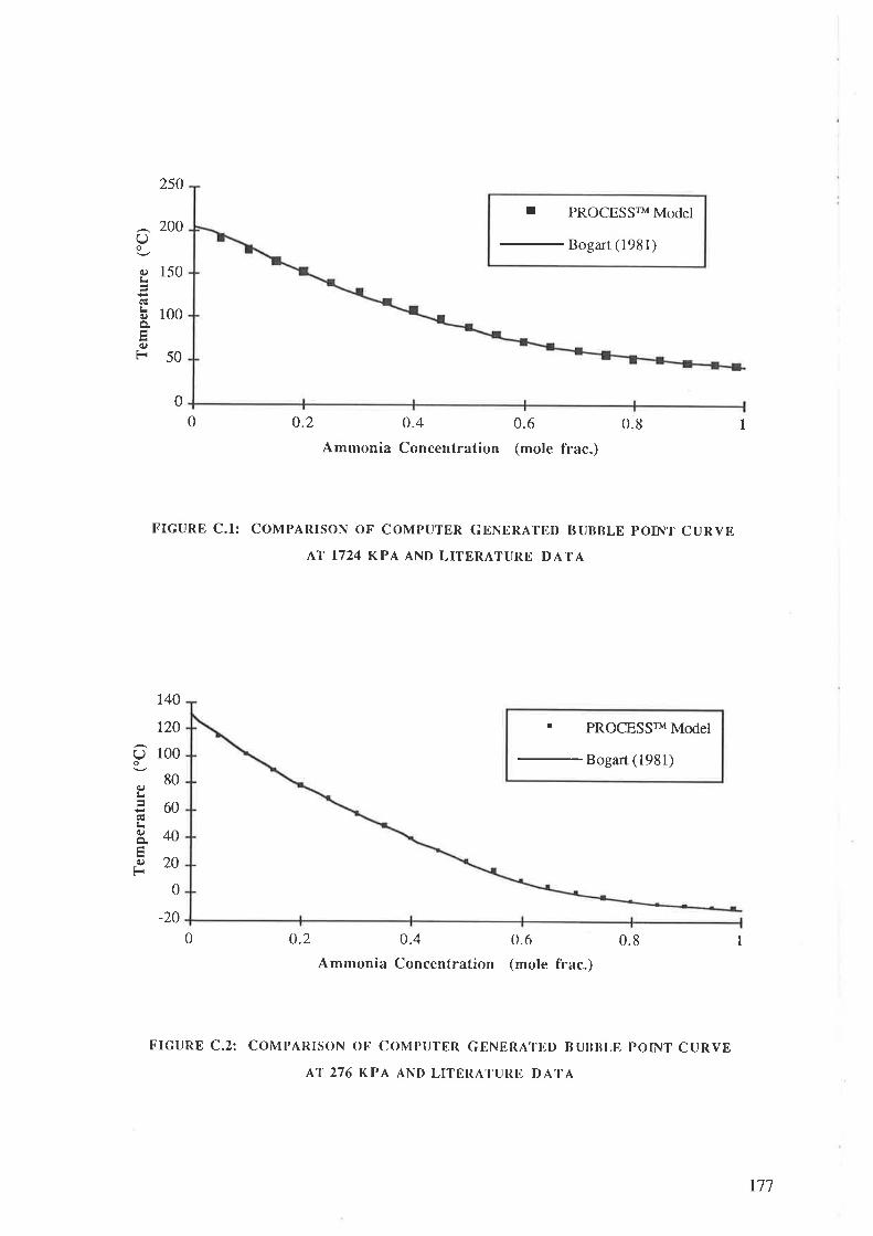
250
200
150
100
50
Qo
(¡)
cg
(u
c)3
0.2 0.4
Ammonia Concentration
r PROCESSTM Model
Bogart (1981)
0.6
(mole frac.)
0
0.8
FIGURE C.1: COMPARISON OF COMPUTER GENERATBD I}UBBLE POINT CURVE
AT 1724 KPA AND LITERATURE DATÂ
' PROCESSW Model
-Bogart
(1981)
-20
0 0.2 0.4
Ammonia Concentration
0.6
(mole frac.)
0.8
FIGURE C.2: COMPARISON OF COMPUTER GENERATED BUBIJLB POINT CURVE
AT 276 KPA AND LITERATURE DATA
0 1
140
120
100
80
60
40
20
0
Oo
q)
q)qq)
F
I
t7l

Program Listings
SUBROUTINE UKHS2C ** This subroutine calculates k values for the arrrmonla water systern
C ** based on the equation of state proposed by Ziegler & Trepp
COMMON ÆACTOR/ TCONVT,TFAC, PCONVT,PFAC,TIMFAC,WTFAC,VVFAC,* ARFAC,XLVFAC,SPGFAC,HSFAC,WKFAC,VISFAC,TCFAC,VVFACA,STFAC,* FACA,FACB,EXPFAC,XM3FAC,F|OR,CTOK,XKTOR,ATM,VVTOML,RCONST
COMMON ruTHERMÂFLAG,NOCX,IFAZE, IWATER, IOUT,TEMPR,TDELTR,* pRESR,XV(50),XL(50),XL2(50),YSAT,XSOL,XKAY(50),DRIV(50),HS1,HS2,
* zI,Z2,JFLAG,IFLG(10)
DTMENSTON STREAM(60),VPS (50)
rF(TFLAG.NE.-1) GOTO 10
JFLAG=3
RETURN
10 rF(rFLG(4).Gr.0) GOTO 20
IFLG(4)=1
C *x Assigning values to the equation of state parameters
HLORA=4.878573
HGORA=26.468819
SLORA=1.644173
SGORA=8.339026
TORA=3.2252
PORA=2.0000
HLORV/=ZI.821141
HGORW=60.965058
SLORW=5.733498
SGORW=13.45343
TORW=5.0705
PORW=3.0000
AIA=3.9114238-2
A2A=-1.7905578-5
A3A=- 1.308905E-2
A4A=3.1528368-3
B1A=1 .63451981
B2A=-6.508119
B3A=1.448931
178
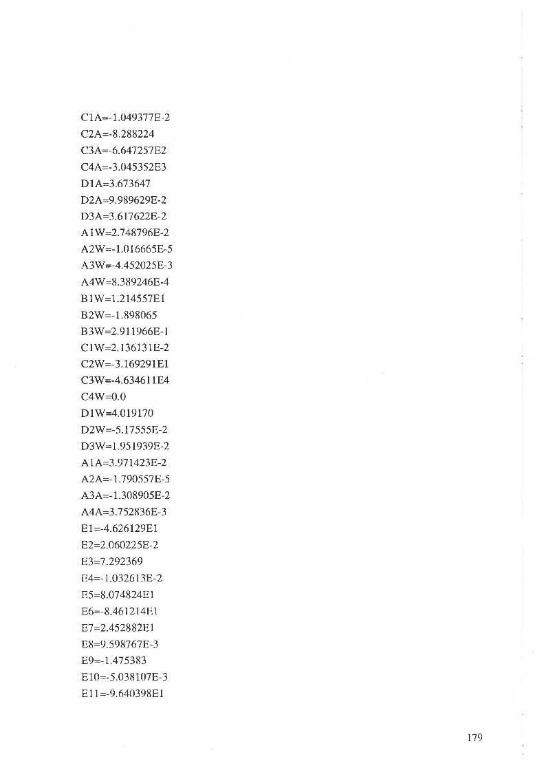
C1A=-1.0493718-2
C2A=-8.288224
C3A:-6.64125182
C4A=-3.045352E.3
DIA=3.613641
D2A:9.9896298-2
D3A=3.6176228-2
AlW=2.7481968-2
A2W=-1.016665E-5
A3W=-4.4520258-3
A4W=8.3892468-4
BIW=1.21455781.
B2W=-1.898065
B3W=2.9119668-1
CIW=2.1361318-2
C2W=-3.1692918I
C3W=-4.634611F4
C4W=0.0
DIW=4.019170
D2W=-5.175558-2
D3W=1.9519398-2
AlA=3.9714238-2
A2A=-1.790557E-5
A3A:-1.3089058-2
A4A=3.7528368-3
El=-4.62612981
E2=2.0602258-Z
E3=7.292369
E4:-L0326138-2E5=8.01482481
E6=-8.4612148I
E]=2.45288281
E8=9.5987678-3
E9=-1.475383
810=-5.038107E-3
Ell=-9.64039881
179

EI2=1.22697382
813=-7.582637
El4=6.0124458-4
El5=5.48701881
EI6=-1.66159681
20 rF(rFLAG.EQ.0) RETURN
rF(IFLAG.EQ.l) GOrO 30
JFLAG=99
wRrTE(rouT,60) rFLAG
60 FORMAT(5OHO ** FATAL ERROR -USER THERMO U2 IS KVALUES-IFLAG=,I5)
RETURN
30 II=0
C ** Converting frorn prograrn units to SI units
TD EGK= CI-EMP R+TC Ol{-\rD x TFA CIXKTOR
Pg 6P=(PRES R+PCONVÐ *PFA Cl 14.50
TR:TDEGIV100
PR=PBAR/I0
C ** Calculating the normalised liquid phase Gibbs Free Energy of Ammonia
40 GLRA=HLORA_TR*SLORA+B 1A*TRaþ)tr//*tR*x2+B3A/3*TR**3_* B1A*TR*LOG(|R)
GLRA:GLRA-B2A*TR* *2-83 N2*TR**3-B 1 A*TORA-B 2 NZ*TORI\* * 2-
* B3A/3*TORA*'<3
GLRA{LRA+TR*B IA*LOG C|ORA)+B2A*TR*TORA +83 N2*TR*TORA**2GLRA=G LRA+(A 1A+A3A*TR+A4A *TR* *2) *(pR_pORA)+A2A* (pR* *2_POP.A* *2)12
C x* Calculating the normalised liquid phase Gibbs Free Energy of Water
GLRW=HLORW-TR* S LORW+B 1 W*TR+B2V#2*TR* x2+B 3 W3 *TR* x3-
* B 1W*TR*LOG(TR)
GLRW=GLRW_B2W*TR* *2-B3W2¿<TR*x3-B 1W*TORV/ -B2W ¡2*'¡ORW**2-x B3V//3*TORV/**3
GLRV/=GLRV/+TR*B 1 W*LOG(TORW)+B2W*TR*TORW+B 3W2*TR*TORW'k>F2
GLRW=GLRW+(A 1 W+A3V/*TR+A4W*TR* *2)* (pR_PORW)+A2W,', (pR* *2_
* PORS¡**/)/2
180
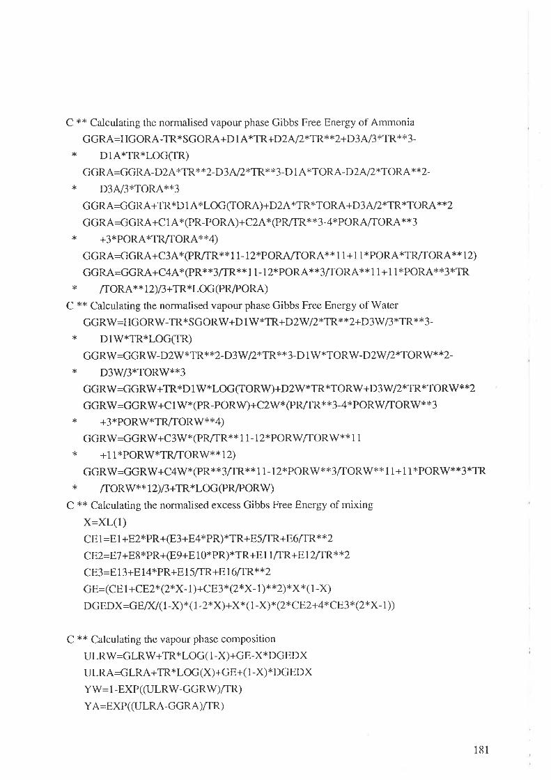
C ** Calculating the normalised vapour phase Gibbs Free Energy of Ammonia
GGRA:HGORA-TR*SGORA+D 1 A*TR+D2fu2>FTR**2+D3A/3 *TRx* 3-
* DIA*TR*LOG(I-R)
GGRA=GGRA_D2A*TR* *2_D3 NL*TR* *3_D 1 A*TORA_D2NZ*T ORA* * 2_
x D3A/3*TORA**3
GGRA=GGRA+TR*D 1 A *LOG CIORA)+D2A *TR*TORA+D3 A/2*TR *TORA * *2
GGRA=GGRA+C I A*(PR-PORA)+C2A* (PR/|R* *3-4* PORAffgB¡ * *3
x +3*PORA*TRr|ORA**4)
GGRA=GGRA+C3A*(PR/TR* x 1 1 - I 2*PORAÆORA * * 1 1 + 1 1 * PORA *TR/TOR A* * 12)
GGRA=GGRA+C4A* @R* *3/TR** 1 1 - 1 2*PORA* *3ÆORA* * 1 1 + 1 1 * PORA'k *3 *TR
* ffORA**72)13+TR*LOG(PR/PORA)
C x* Calculating the normalised vapour phase Gibbs Free Energy of Water
GG RW=HGORW-TR* S G ORW+D 1 W*TR+D2W2*TR * * 2+D3W 13 *TR* * 3-
* D1W*TR*LOG(IR)
GGRW=GGRV/_D2W*TR* x2-D3V//2*TR**3_D 1 W*TORW_D2W2*TORW* *2_
* D3W3*TORV/**3
GGRW=GGRW+TR*D I W*LOG CTORW)+D2W*TR*TORV/+D3 W2*TR*TORW''{<2
GGRW=GGRW+C 1 W*(PR-PORV/')+C2W* @R/TR* *3-4*PORWTORW* x3
x +3*PORW*TR/TORW**4)
GGRW=GGRW+C3W* (PRÆR* * 1 I - 1 2* PORWff QBy¿* * 1 1
x +lI*PORW*TR/TORW**12)
GGRW=GGRW+C4W*(PR**3ÆR** I 1- l2*PORW**3ÆORW** 11+ 1 1*PORW**3*TR* /IORW**12)/3+TR*LOG(PR/PORIV)
C ** Calculating the normalised excess Gibbs Free Energy of mixing
X=XL(1)
CE 1 =E 1 +E2*pR+@3+E4x pR)*TR+85ÆR+E6ffRx *2
CE2:87 +88 x PR+ @ 9+E 1 0 * PR) *TR+E I 1 ÆR+ E 1 2íf R * * 2
CE3=E 1 3+E 14*PR+E 1 5ÆR+E 1 6ÆR* *2
G E= (C E 1 + çE2* (2*X- 1 ) +C E 3 * (2* X- l) * * 2) * X * ( 1 - X )
DGEDX=GEDí( 1 -X)*( 1 -2*X)+X* (1 -X)*(2* CE2+4* CE3 x (2*X- I ))
C ** Calculating the vapour phase composition
ULRW=GLRW+TR* LOG ( I -X)+GE-X* DGEDX
ULRA=G LRA+TR*LOG (X)+G E+( 1 -X)* DGEDX
YW: 1 -EXP((ULRW-G GRW)ÆR)
Y A=EXP((ULRA-GGRA)/TR)
181

C ** Calculating the equilibriurn K values and the temperature derivative
XK1=YA/XL(1)
XK2=Y'W/(1-XL(1))
TFCTDELTR.EQ.0.) GOTO 77
rF(rr.GT.0) GoTo 50
II:II+1XKAY(1)=XK1
XKAY(2)=XK2
TR=CTDEGK+0.01)/100
GOTO 40
50 DR[V( 1)=CXK1-XKAY(1))/0.0 1
D RrV(2) =CXK2-XKAY (2)) /0.0 t
77 CONTINUE
RETURN
END
182

SUBROUTINE UKHS3
C *xx* This subroutine calculates H values for the alnmonia water system
C t<'k** based on the equation of state proposed by Ziegler & Trepp
COMMON /FACTOR/ TCONVT,TFAC,PCONVT,PFAC,TIMFAC,WTFAC,WFAC,* ARFAC,XLVFAC,SPGFAC,HSFAC,WKFAC,VIS FAC,TCFAC,VVFACA,STFAC,CA,* FAFACB,EXPFAC,XM3 FAC,F|OR,CTOK,XKTOR,ATM,VVTOML,RCONST
COMMON ruTHERMÆFLAG,NOCX,IFAZE, IWATER, IOUT,TEMPR,TDELTR,x PRESR,XV(50),XL(50),XL2(50),YSAT,XS OL,XKAY(50),DRIV(50),HS 1,HS2,
* zl,Z2,JFLAG,IFLG( 10)
JFLAG=1
rF(rFLAG.EQ.2) GOrO 10
V/RITE(IOUT,90) rFLAG
90 FORMAT(48H0***ERROR-USER METHOD U3 IS ENTHALPIES - IFLAG:,ISJI)
JFLAG=99
RETURN
C ** Assigning values to the equation of state pa-ralneters
10 HLORA=4.878573
HGORA=26.468879
SLORA=1.644773
SGORA:8.339026'Í.ORA=3.2252
PORA=2.0000
HLORW=LI.821141
HGORW:60.965058
SLORW=5.733498
SGORW:13.45343
TORW=5.0705
PORW=3.0000
ÃlA=3.9114238-2
A2A=-1.190551F-5
A3A=- 1.308905E-2
A4A=3.7528368-3
B1A=1 .63451,981
B2A=-6.508119
B3A=1.448937
183

C 1A=- 1.0493718-2
C2A=-8.288224
C3A=-6.64725782
C4A=-3.04535283
DIA=3.673647
D2A=9.9896298-2
D3A=3.6176228-2
AIW=2.1487968-2
A2W=-1.0166658-5
A3W=-4.4520258-3
A4W=8.3892468-4
BIW=1.2145518I
B2'W=-1.898065
B3rW=2.911966E-1
CIW=2.1361318-2
C2W=-3.1692978I
C3W=-4.63461184
C4V/=0.0
D1W=4.019170
D2W=-5.175558-2
D3W=1.9519398-2
E7=-4.62612981
E2=2.0602258-2
E3=7.292369
E4=-1.032613F-2
E5=8.07482481
E6=-8.46121487
E7=2.45288281
E8=9.5987678-3
E9=-1.475383
810=-5.0381078-3
Ell=-9.640398E1
EI2=1.226973E,2
El3=-7.582637
El4=6.0124458-4
El5=5.481018E1
El6=-7.66159681
184
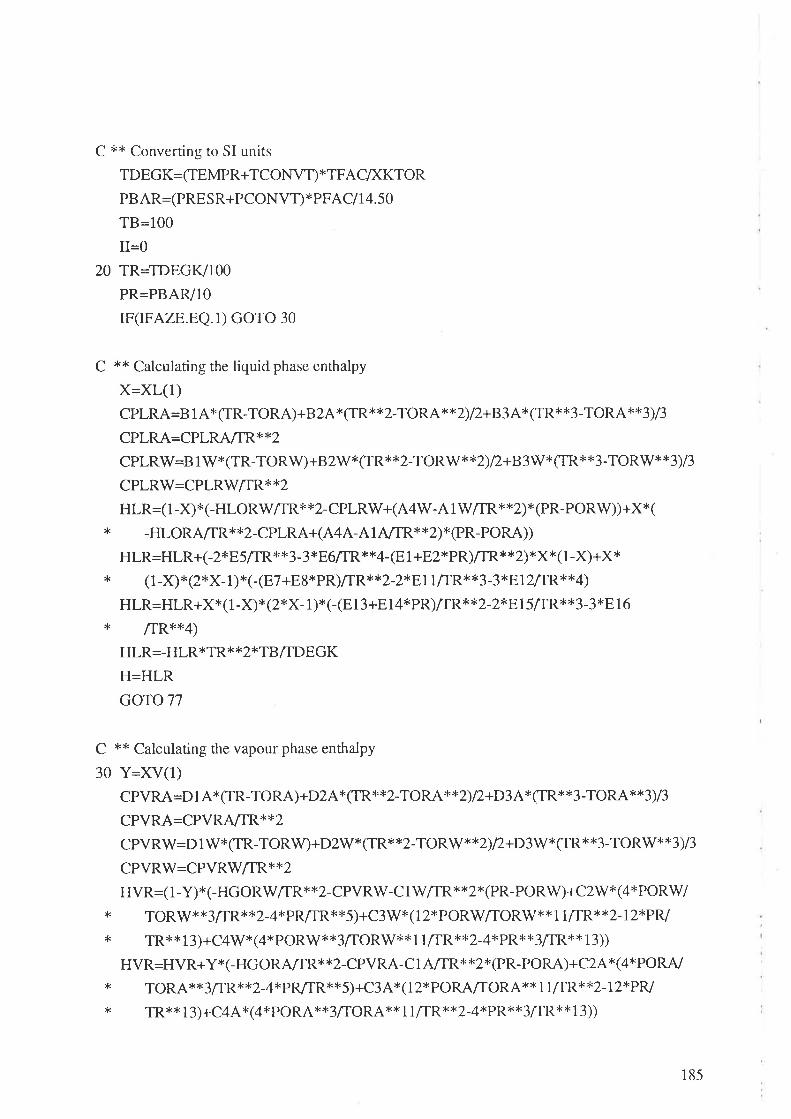
C xx Converting to SI units
TDEGK=(|EMPR+TCONVT) *TFACIXKTOR
Pg AP:(PRES R+PCONVÐ * PFA Cl 14.50
TB=100
II=0
20 TR=TDEGIVIO0
PR=PBAR/10
rF(rFAZE.EQ.1) GOTO 30
C ** Calculating the liquid phase enthalpy
X=XL(1)
CPLRA=B 1 4x ¡[R-TORA)+B2AxCfR** 2-TORI\**Z) l2+83 Ax (TR**'<3-TO&\*'<3)/3
GPLRA=CPLRA/TR**2
CPLRW=B 1 V/*(TR-TORW)+B2W*(f R* *2-TORW* *2) l2+B3W x fl-R* *3-TORW* *3)/3
GPLRW=CPLRTçV/TR**2
HLR=( 1 -X)*(-HLORWÆR* *2-CPLRW+(A4W-A lWffR*x2)x(PR-PORW))+X*(* -HLORAÆR**2-CPLRA+(A4A-AlATTR**2)*(PR-PORA))
HLR=HLR+(-2*E5[R**3-3{'.E6flR**4-(E I +E2xPR)/TR**2)*X*(1-X)+X*x (1-X)'.(2xX-1)*(-(E7+eSxPR)/TR**2-2*E71ffR**3-3*E12flR*'k4)
HLR=HLR+{*(l -{)x (2*X- 1 )* (-(E 1 3+E I 4*PR)ftR* *2-2xE I 5ÆR>k * 3-3 *E 1 6
* ÆR**4)HLR=_HLR x TR * * 2* TB rfD E GK
H=HLR
GOTO 77
C ** Calculating the vapour phase enthalpy
30 Y=XV(l)CPVRA=D 1 4x GR-TORA)+D2A*(TR*x2-TORl\*>kZ)/2+D3A*(fRx *3-TO&{**3)/3
CpVRA=CpVRy'vTR*x2
CPVRW=D 11y*1TR-TORW)+D2W* (lR**2-TORW* *2) /2+D3W *(TR* *3-TORW* x3)/3
GPVRW:CPVRWT|R**2
¡¡yp=( I -Y)t' (-HGORWTR*x2-CPVRW-C 1 Wfl-R* *2*(PR-PORW)+C2W* (4*PORW* TORW**3flR>k*2-4*PR/fR**5)+C3W*(12*PORWf|ORV/**1 1/TRi'<*<2-12*PR/
* TR**13)+C4V/*(4xPORW*x3¡ORW**1 1/TR*c*2-41<PRx*3ffR*x13))
HVR=HVR*yx1-HG ORJ{,/TRI< *2-CPVRA-C 1 A/TR* *2*(PR-PORA)+C2 A* (4*PORA/
* TORAx*3ÆR*{,2-4xPR/TR)I*5)+C3A*(12*PORAÆORA*x11ffR*x2-12xPR/* TR**13)+C4Ax(4*PORA**3/TORA**11ffR**2-4xPR*'k3lTR**13))
185

HVR=-HVR *TR * *2xTBlTD EG K
H=HVR
77 CONTINUE
II=II+ 1
TDEGK=TDEGK+TDELTR
rF(rr.EQ.2) GOrO 40
HS1:H
C ** Calculating the enthalpy at a small increment higher temperature
GOTO 20
40 HS2=H
RETURN
END
186

SUBROUTINE UKHS4
C ** This subroutine calculates entropy values for the ammonia water system
C ** based on the equation of state proposed by Ziegler & Trepp
COMMON ÆACTOR/ TCONVT,TFAC,PCONVT,PFAC,TIMFAC,WTFAC,VVFAC,* ARFAC,XLVFAC,SPGFAC,HSFAC,WKFAC,VISFAC,TCFAC,VVFACA,CA,* STFAC,FA,FACB,EXPFAC,XM3FAC,FTOR,CTOK,XKTOR,ATM,* VVTOML,RCONST
COMMON N¡f TTENTT'TÂFLAG,NOCX,IFAZE, IWATER, IOUT,TEMPR,TDELTR,* PRESR,XV(50),XL(50),XL2(50),YSAT,XSOL,XKAY(50),DRIV(50),HS1,* HS2,ZI,Z2,JFLAG,IFLG(10)
JFLAG=1
rF(rFLAG.EQ.3) GOTO 10
wRrTE(rottT,99) rFLAG
99 FORMAT(48H0***ERROR-USER METHOD U4 IS ENTROPIES - IFLAG=,[ÍJ|)
JFLAG=99
RETURN
C ** Assigning values to equation of state parameters
10 HLORA=4.818573
HGORA=26.468879
SLORA=1.644713
SGORA=8.339026
TORA=3.2252
PORA=2.0000
HLORW=Z7.821141
HGORW=60.965058
SLORW=5.133498
SGORW=13.45343
TORW=5.0705
PORW=3.0000
A1A=3.9114238-2
A2A=-1.790557E-5
A3A=- 1.3089058-2
A4A=3.1528368-3
B1A=1 .63451981
B2A=-6.508119
B3A=1.448937
187

C1A=-1.0493178-2
C2A,=-8.288224
C3A=-6.64725182
C4A:-3.04535283
DIA=3.613647
D2A=9.9896298-2
D3A=3.6176228-2
AIW=2.7487968-2
A2W=-1.016665E-5
A3W=-4.4520258-3
A4W=8.3892468-4
B1V/=1.21455781
B2\ü/=-1.898065
B3W=2.911966E-1
C1W=2.1361318-2
C2W:-3.16929181
C3lñ/:-4.634611E4
C4'W=0.0
D1W=4.019170
D2W:-5.175558-2
D3W=1.9519398-2
El:-4.6261298L
E2=2.0602258-2
E3=7.292369
E4=-I.0326138-2
E5=8.0148248I
E6=-8.46121481
E7=2.45288281
E8=9.598767E-3
E9=-I.475383
E10=-5.038107E-3
Ell=-9.64039881
El2=1.22691382
El3=-7.582637
EI4=6.0124458-4
El5=5.48701881
El6='l.66759681
188

TDEG K=Cf EMPR+TCONVT) *TFA C/XKTOR
Pg 4P=(PRES R+PCONVÐ * PFA Cl I 4.50
TB=100
II=0
20 TR=TDEGIVI0O
PR=PBAR/l0
rF(rFAZE.EQ.1) GOTO 30
C ** Calculating the liquid phase entropy
X=XL(1)
CpLRA=B 1 AxLOGCIR/TORA)+B2A* (TR-TORA)+B 3A * (TR*x 2-TORA* *2)/2
CPLRW=B 1V/*LOG(TRI|ORW)+B2\M* (TR-TORW)+B 3W* (TR* *2-T OP.W * *2)/2
SLR=( 1 -X)* (-SLORW-CPLRW+(A3W+2 * A4W*TR) *(PR- PORW))+X* (-S LORA* _cpLRA+(A3A+2*A4A*-fR)*(pR_PORA))
SLR=SLR+(E3+E4*P*-ttfa** *2-2*E6ffR**3)*X*( 1 -X)+Xx (1-X) *(2*X- 1)
x x(E9+E10xPR-El1ffRx*2-z*EIz[TP.**3)+X*(1-X)*(2*X-1)x*2*
x (-E15 fI\*>k2-2*E16rl-R**3)SLR=-SLR
H=SLR
GOTO77
C ** Calculating the vapour phase entropy
30 Y=XV(l)CPVRA=D I A*LOGCIR/TORA)+D2A* (|R-TORA)+D3A* (TR* *2-TOR-{* x)) 12
CPVRW=D IW*LOG C|R/TORW)+Ot'ù/*1TR-TORW)+D3W* OR* * 2-T OP.W * *2) /2
5yp=(1-Y) *(-SGORW-CPVRW+LOG (PR/PORW)+C2y¿i'llxPORWÆORW* * 4-3** PRÆR**4)+C3W*(1 1*PORWÆORW**12-ll*PR/TR*r<12)+C4W*(1 1*PORW*{'3x /ToRw**12-11*PR*x3rt-R**t2))
S VR=S VR*yx1-S GORA-CPVRA+LOG (PR/PORA)+C2A*(3 *PORA/TORA *1'<4-3*
* pR/TR**4)+C3A*(1 1*pORpv¡IORA** 12_ t 1*pRffR**12)+C4A*(l 1*PORA**3* rloRA**I2-I1*PR>ß,k3lTR**12))
SVR=-SVR
H=SVR
189

77 CONTINUE
II=II+1TDEGK=TDEGK+TDELTR
rF(rr.EQ.2) GOTO 40
HS1:H
C ** Calculating the entropy at an incrementally higher temperature
GOTO 20
40 HS2:HRETURN
END
190

Appendix D
SAMPLB PROCBSS INPUT AND OUTPUT FILES
The amount of information generated from the numerous computer simulations is too large to
include in its entirety. Instead a number of representative files have been included. These are:
(i) Input and output files for the basic novel refrigeration cycle with methyldiethylamine and
water as working fluids.
(ii) Input and output files for the novel refrigeration cycle with absorbent phase distillation
employing dimethylethylamine and water as working fluids.
(iii) Input and ouþut files for the modified aqua-ammonia refrigeration cycle without
precooling.
(iv) Input and output files for the conventional aqua-ammonia refrigeration cycle without
precooling.
(v) Input and output hles for the basic novel absorption cycle heatpump with cyclohexane and
aniline as working fluids.
191

PROCESSru Input and Output File Listinss
BASIC NOVEL REFRIGERATION CYCLE WITH
METHYLDIETHYLAMINE AND WATER
192

TITLE PROJECT=MDEAM REFRIG, DATE=8-7 -90
CALC NOTRIAL=I0
TOLERANCE PROP=O.0005,TEMP=-0.002,5TREAM=0.000 1,-0.002
DIM ENSION S I,TEMP=C,PRES S URE=MMHG
PRINT INPUT=NONE
COMP DATA
LIBID 2,H2O
NONLIBRARY I,MDEAMIMV/ 1,87.17
SPGR I,0.72
NBP 1,66
TC 1,235
PC 1,25091
ACENTRIC 1,0.3039
FORMATION(KJ,KG) r,-l 9,102.0
VP(MMHG ) CORR=2 l,LOG,TEMP=C,DATA= 1,,,6. 9 1 57 8,- 1 18 4.8,227 .67
HIDEA L(KJ,KG, MOLE) CORR= 1,TEM P=K, DATA= 1,,,+ | 6.447,- IZ.3 488-3,*
0. 30 1 3 8E-3,-t.2027 E-7,2.14258-t r
LATENT(KJ,KG) CORR=43,TFM P=K, D ATA= 1,,,33 6.2,0.38
HLIQ(KJ,KG,MOLE) CORR= 1,TEMP=C,DATA= 1,,,0 .0,0.2022
THERMO DATA
TYPE KTYP=LACT,LACT,HTYP:LIB RARY,STYP=S RK
HLSET KSET=1,SETNO=1
KSET SETNO=l,NOTEMP=3
SUBSET 1,10
NRTL 1,2,,20J .7 J 90,,586.120 1,0.502 1 3
SUBSET 2,30
NRTL r,2,,468.6817,,8 10.0509,0.502 1 3
SUBSET 3,5O.OO
NRTL 1,2,,729.5844,,1033.98 17,0.5021 3
KSET SETNO=2
NRTL 1,2,,67 4.6857,,131 9.9828,0.4 108
STREAM DATA
PROPERTY STRM=3,TEMP=80,PRES :2500,RATE =I542,COMP:I,I.08/2,98.92PROPERTY STRM= 1 2,TEMP=2O,PRES:2500,RATE:1 52 1,CO}l4P=I,4.4212,95.58
PROPERTY STRM=4,TEM P=80, PRES :2500, RATE=3 28, COMP=I,65.0 12,3 5.0
PROPERTY STRM:9,TEM P= 1 0, PRES :2500,R4T8=29 8, COMP = 1,60.7 12,39.3
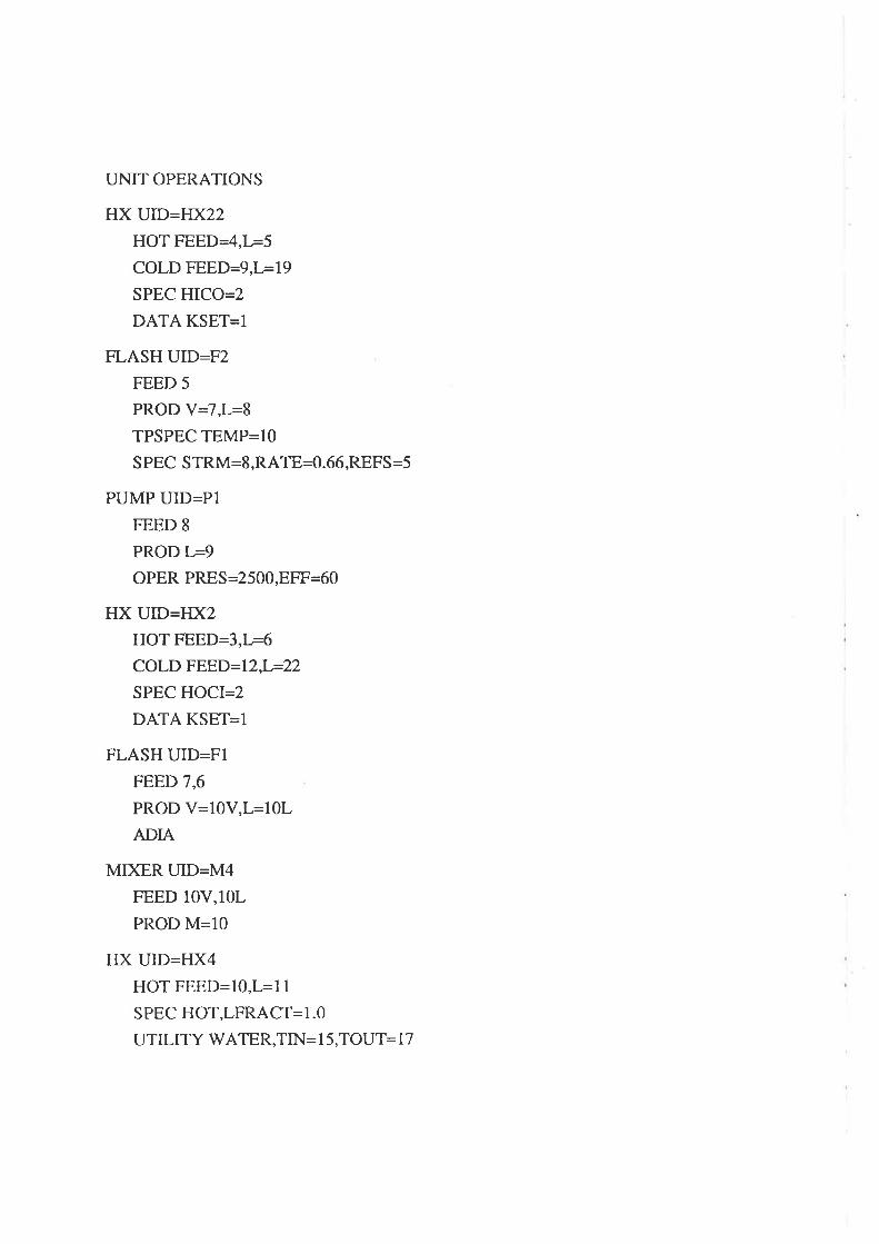
UNTI OPERATIONS
HX UID=HX22
HOT FEED_4,1.5
COLD FEED=9,L=19
SPEC HICO=2
DATA KSET=I
FLASH UID=F2
FEED 5
PROD V=7,L=8
TPSPEC TEMP=l0
S PEC STRM:8,RATE4.66,REFS=5
PUMP UID=PI
FEED 8
PROD L=9
OPER PRES:2500,EFF=60
HX UID=HX2
HOT FEED-3,T:6COLD FEED=12,L=22
SPEC HOCI=2
DATA KSET=I
FLASH UID=FIFEED 7,6
PROD V:10V,L=10L
ADIA
MIXER UID=M4
FEED IOV,IOL
PROD M=10
HX UID=HX4
HOT FEED=10,L=11
SPEC HOT,LFRACT=I.0
UTILITY WATER,TIN= I 5,TOUT :17

PUMP UID=P2
FEED 1 1
PROD L=12
OPER PRES=2500,8FF=60
CONTROL UID:CONISPEC STRM=I1,TEMP=20
PARAM STRM=3,MAXI= 1 50000,MINI= 1 00,EST2= 1 2O0,RETURNUMT=HX2
MIXER UID=M3
FEED 22,19
PROD l/{43
SEPARATOR UID=S 1
FEED 23
OVHD STRM=4,PHAS E=L,TEMP=80
BTMS STRM=3,TEMP=80
xovHD 1,1,0.65
XBTMS 2,2,0.989
RECYCLE
LOOP NO= I,START=HX22,END=P I
LOOP NO=2,START:HX2,END=P2
LOOP NO=3,START=HX22,END=S 1
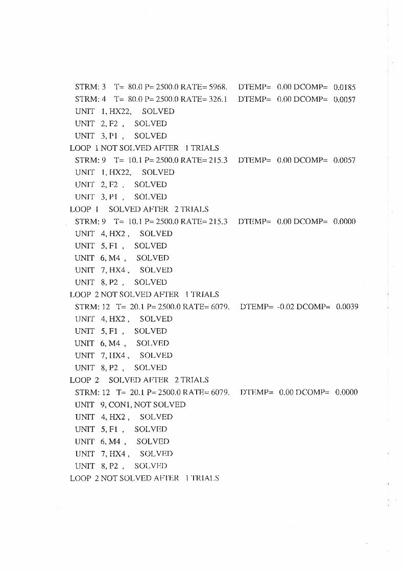
STRM: 3 T= 80.0 P= 2500.0 RATE= 5968.
STRM: 4 T= 80.0 P= 2500.0 RATE= 326.1
UNTT I,HX22, SOLVED
UNIT 2,F2 , SOLVED
UNIT 3, Pl , SOLVED
LOOP 1 NOT SOLVED AFTER 1 TRIALS
STRM: 9 T= 10.1 P= 2500.0 RATE= 215.3
UNTI T,HX22, SOLVED
UI\IIT z,FZ , SOLVED
UNIT 3, P1 , SOLVED
LOOP 1 SOLVED AF|ER 2 TRIALS
STRM: 9 T= 10.1 P= 2500.0 RATE= 215.3
UNIT 4,HX2, SOLVED
UNIT 5, F1 , SOLVED
Ul\tIT 6,M4 , SOLVED
UNIT 7 ,}lX4, SOLVED
UNIT 8,P2 , SOLVED
LOOP 2 NOT SOLVED AF|ER 1 TRIALS
STRM: 12 T= 20.1P= 2500.0 RATE= 6079
UNTT 4,TfX2, SOLVED
UNIT 5, F1 , SOLVED
UNIT 6,M4 , SOLVED
UNTI 7,HX4, SOLVED
UNIT 8,P2 , SOLVED
LOOP 2 SOLVED AFTER 2 TRIALS
STRM: 12 T= 20.1 P= 2500.0 RATE= 6079
UNIT 9, CONI, NOT SOLVED
UI\IIT 4,ffx2, SOLVED
UNIT 5, Fl , SOLVED
UNIT 6,M4 , SOLVED
UNIT 7 ,HX4, SOLVED
UNIT 8,P2 , SOLVED
LOOP 2 NOT SOLVED AF|ER 1 TRIALS
DTEMP= 0.00 DCOMP= 0.0185
DTEMP= 0.00 DCOMP= 0.0057
DTEMP= 0.00 DCOMP= 0.0057
DTEMP= 0.00 DCOMP= 0.0000
DTEMP= -0.02 DCOMP= 0.0039
DTEMP= 0.00 DCOMP= 0.0000

STRM: 12 T: 20.1 P= 2500.0 RATE= 6077.
UNIT 4,HX2, SOLVED
UNIT 5, Fl , SOLVED
UNIT 6,M4, SOLVED
UNIT ],HX4, SOLVED
UNIT 8,P2, SOLVED
LOOP 2 SOLVED AFTER 2 TRIALS
STRM: 12 T= 20.1 P= 2500.0 RATE= 6077.
UNTI 9, CONI, NOT SOLVED
UNIT 4,HX2, SOLVED
UNIT 5, Fl , SOLVED
UNIT 6, M4 , SOLVED
UNTT 7,IlX4, SOLVED
UI\IIT 8,P2, SOLVED
LOOP 2 NOT SOLVED AFTER 1 TRIALS
STRM: 12 T= 2O.I P= 2500.0 RATE= 6125.
UNTI 4,HX2, SOLVED
UNIT 5, Fl , SOLVED
Ul\tIT 6,M4 , SOLVED
UNTI ],HX4, SOLVED
UNIT 8, P2 , SOLVED
LOOP 2 SOLVED AF-|ER 2 TRIALS
STRM: 12 T= 20.1 P:2500.0 RATE= 6125.
UNTI 9, CONI, SOLVED
UNIT 10, M3 , SOLVED
UNIT 11, 51 , SOLVED
LOOP 3 SOLVED AF-|ER 2 TRIALS
STRM: 3 T= 80.0 P= 2500.0 RATE= 6014.
STRM: 4 T= 80.0 P= 2500.0 RATE= 326.1
DTEMP= 0.00 DCOMP= 0.0003
DTEMP= 0.00 DCOMP= 0.0000
DTEMP= 0.03 DCOMP= 0.0080
DTEMP= 0.00 DCOMP= 0.0000
DTEMP= 0.00 DCOMP= 0.0000
DTEMP= 0.00 DCOMP= 0.0000

**** PROBLEM SOLUTION REACHED xr<**
VERSION 0,484 SM
SIMULATION SCIENCES,INC. PROCESS
PROJECT MDEAM REFRIG
PROBLEM SOLUTION 8-7-90
PAGE 4
SUMMARY OF FLASH DRUMS,MDGR/SPLITTERS AND VALVES
UNIT ID
SEQ NO
TYPE
FEEDS
PRODUCTS
TEMP, DEG C
PRESSURE, MMHG
FRACTION LIQUID
DUTY, MM KJ /FIR
FZ
2
FLASH
7 (v)
8 (L)
10.0000
61.2398
0.66020
2.2r90t
F1
5
FLASH
7
6
10v (v)
10L (L)
23.5314
67.2398
0.98393
0.00000
M4
6
MIXER
10v
10L
10 (M)
23.5314
61.2398
0.98393
0.00000
M3
10
MIXER
22
t9
23 (L)
73.0058
2500.0000
1.00000
0.00000
5
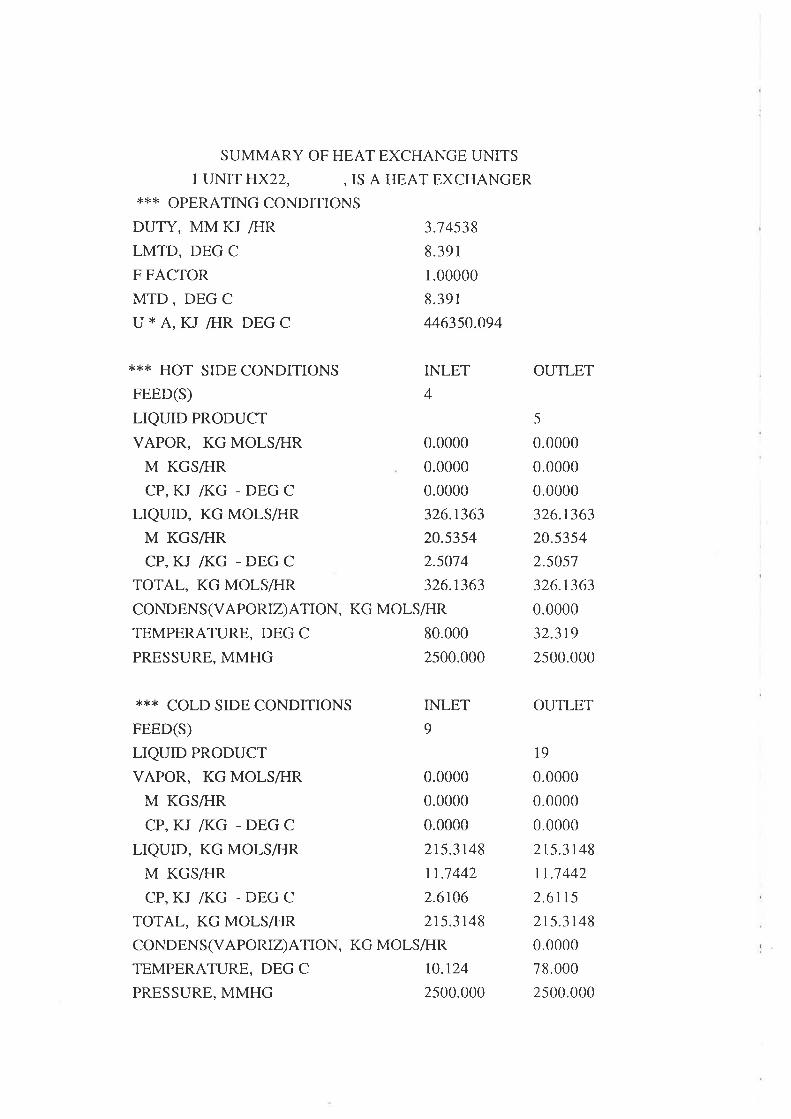
SUMMARY OF HEAT EXCHANGE UNITS
1 UNIT HX22, , IS A HEAT EXCHANGER**X OPERATING CONDITTONS
DUTY, MM KJ /HR 3.74538
LMTD, DEG C 8.391
F FACTOR I.OOOOO
MTD, DEG C 8.391
U * A, KJ ÆIR DEG C 446350.094
**'< HOT SIDE CONDMONS INLET
FEED(S) 4
LIQUID PRODUCT
VAPOR, KG MOLSÆIR O.OOOO
M KGS/HR O.OOOO
CP, KJ Æ(G - DEG C O.OOOO
LIQUID, KG MOLSÆIR 326.1363
M KGSiHR 20.5354
CP, KJ /KG - DEG C 2.5074
TOTAL, KG MOLSÆIR 326.1363
CONDENS(VAPORIZ)ATION, KG MOLS/FIR
TEMPERATURE, DEG C 8O.OOO
PRESSURE, MMHG 25OO.OOO
*,.'< COLD SIDE CONDITIONS INLET
FEED(S) 9
LIQUID PRODUCT
VAPOR, KG MOLSÆIR O.OOOO
M KGS/FIR O.OOOO
CP, KJ A(G - DEG C O.OOOO
LIQUID, KG MOLS/F{R 2r5.3r48
M KGS/HR 1T,1442
CP, KJ Æ(G . DEG C 2.6106
TOTAL, KG MOLSÆ{R 2I5.3I48
CONDENS(VAPORIZ)ATION, KG MOLS/FrR
TEMPERATURE, DEG C TO.T24
PRESSURE, MMHG 25OO.OOO
OUTLET
-5
0.0000
0.0000
0.0000
326.1363
20.5354
2.50s7
326.t363
0.0000
32.319
2500.000
OUTLET
19
0.0000
0.0000
0.0000
2t5.3t48rI.7 442
2.6rr52r5.3r48
0.0000
78.000
2s00.000

4 UNIT HXz , , IS A HEAT EXCHANGER
:K",K OPERATING CONDITIONS
DUTY, MM KJ ÆIR
LMTD, DEG C
F FACTOR
MTD, DEG C
U X A, KJ /FIR DEG C
21.80338
4.37 5
1.00000
4.37 5
6354104.500
*** HOT SIDE CONDITIONS INLET
FEED(S) 3
LIQUID PRODUCT
VAPOR, KG MOLS/HR O.OOOO
M KGS/FIR O.OOOO
CP,zu Æ(G -DEGC O.OOOO
LrQUrD, KG MOLS/ÉIR 6013.9165
M KGSÆIR 112.9155
CP, KJ /I(G - DEG C 4.0988
TOTAL, KG MOLSÆ{R 6013.9165
CONDENS(VAPORTZ)ATION, KG MOLS/FrR
TEMPERATURE, DEG C 8O.OOO
PRESSURE, MMHG 25OO.OOO
X*X COLD SIDE CONDITIONS INLET
FEED(S) 12
LIQUID PRODUCT
VAPOR, KG MOLS/HR O.OOOO
M KGSÆIR O.OOOO
CP, KJ Æ(G - DEG C O.OOOO
LTQUID, KG MOLSÆrR 6124.1388
M KGS/HR 12T.]068
CP, KJ /I(G - DEG C 3.9625
TOTAL, KG MOLS/FIR 6124.7388
CONDENSÕ/APORIZ)ATION, KG MOLS/FIR
TEMPERATURE, DEG C 20.124
PRESSURE, MMHG 25OO.OOO
OUTLET
6
0.0000
0.0000
0.0000
6013.9165
t12.9t554.0859
6013.9165
0.0000
22.I24
2500.000
OUTLET
22
0.0000
0.0000
0.0000
6124.1388
t2t.70683.968 1
6124.7388
0.0000
7 t.851
2500.000
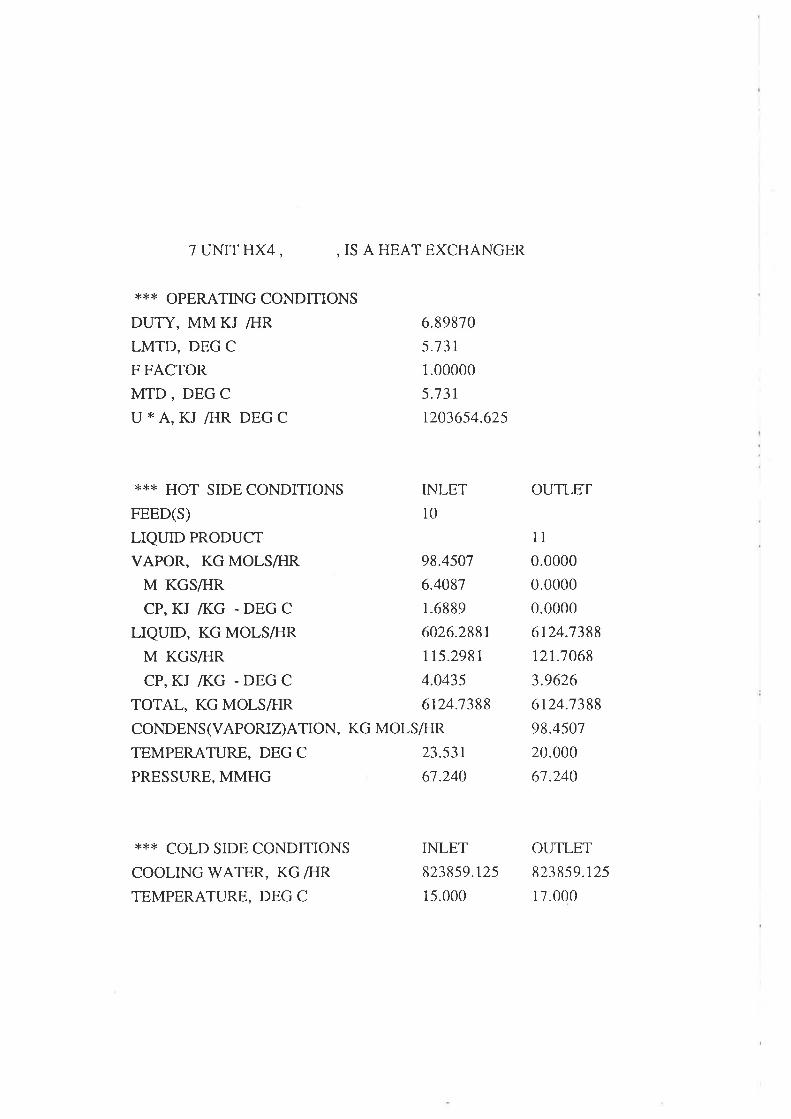
7 UNIT HX4 , , IS A HEAT EXCHANGER
*** OPERATING CONDITIONS
DUTY, MM zu /HR
LMTD, DEG C
F FACTOR
MTD, DEG C
U*A,KJ ÆIR DEGC
X*X COLD SIDE CONDITIONS
COOLING WATER, KG /HR
TEMPERATURE, DEG C
*<** HOT SIDE CONDITIONS TNLET
FEED(S) 10
LIQUID PRODUCT
VAPOR, KG MOLSÆIR 98.4507
M KGS/ÉIR 6.4087
CP, KJ Æ(G - DEG C 1.6889
LrQUrD, KG MOLSÆIR 6026.2881
M KGS/FIR 115.2981
CP, KJ /I(G - DEG C 4.0435
TOTAL, KG MOLSÆIR 6124.1388
CONDENS(VAPORIZ)AÏON, KG MOLS/FIR
TEMPERATURE, DEG C 23.537
PRESSURE, MMHG 61.240
6.89870
5.131
1.00000
5.731
1203654.625
INLET
8238s9.t25
15.000
OUTLET
il0.0000
0.0000
0.0000
6124.7388
t2t.1068
3.9626
6124.7388
98.4507
20.000
61.240
OUTLET
823859.r25
17.000

SUMMARY OF COMPRESSORÆXPANDERÆUMPÆURBINE UNTIS
3 UNIT PI , , IS A PUMP**¡K FEED STREAMS ARE 8
*** LIQUID PRODUCT IS STREAM 9X** OPERATING CONDITIONS
V/ORK, KW
EFFICIENCY, PERCENT
MOLE FRACTION LIQUID
TEMPERATURE, DEG C
PRESSURE, MMHG
HEAD, M
HOT VOLUME, M3ÆIR
8 UNIT P2 , , IS A PUMP**,* IüED STREAMS ARE 11
*** LIQUID PRODUCT IS STREAM 12
X"* OPERATING CONDMONS
V/ORK, KW
EFFICIENCY, PERCENT
MOLE FRACTION LIQUID
TEMPERATURE, DEG C
PRESSURE, MMHG
HEAD, M
HOT VOLUME, M3/FIR
INLET
1.0000
10.000
67.2398
t5.546
2.33
60.00
19.24
60.00
OUTLET
1.0000
t0.r242500.0000
12.9743
r5.546
INLET
1.0000
20.000
61.2398
OUTLET
1.0000
20.r24
2500.0000
58.0193
r28.092128.086

UNIT ID
SEQ NO
FEEDS
SUMMARY OF COMPONENT SEPARATORS
S1
11
23
PRODUCTS
TEMP, DEG C
PRESSURE, MMHG
FRACTION LIQUID
DUTY, MM KJ /HR
4 (L) 3 (L)
80.0000 80.0000
2500.0000 2500.0000
1.00000 1.00000
-4.60207
STREAM COMPONENT FLOW RATES -
STREAM ID 3 4
PHASE LIQUID LIQUID
I MDEAMr 66.152s 21t.990r
2IJ20 s941.16t7 tr4.r489TOTALS 6013.9141 326.1390
TEMPERATURE, DEG C SO.OOOO SO.OOOO
PRESSURE, MMHG 25OO.OOOO 25OO.OOOO
H, MM KJ /FIR 36.3002 4.6981
MOLE FRACT LTQUTD 1.0000 1.0000
RECYCLE COI.IVERGENCE 0.0000 0.0000
KG MOLSÆIR
56LIQUID LIQUID
Lrt.9889 66.1531
rr4.r4t 5 5941 .1632
326.1363 6013.9165
323190 22.1237
2500.0000 2500.0000
0.9532 8,4968
1.0000 1.0000
0.0000 0.0000
STREAM ID
PHASE
l MDEAMI
2H20
1
VAPOR
98.2549
12.5673
8
LIQUID
tt3.134010 r.5802
9
LIQUID
113.7340
l0l .5802
10
MD(ED
164.4080
s960.3306

TOTALS
TEMPERATURE, DEG C
PRESSURE, MMHG
H, MM zu /FIR
MOLE FRACT LIQUID
RECYCLE CONVERGENCE
STREAM ID
PHASE
l MDEAMI
2Hzo-
TOTALS
TEMPERATURE, DEG C
PRESSURE, MMHG
H, MM KJ Æ]R
MOLE FRACT LIQUID
RECYCLE CONVERGENCE
t10.8222
10.0000
67.2398
3.9787
0.0000
0.0000
11
LIQLIID
164,4080
5960.3306
6124.7388
19.9996
67.2398
5.5768
1.0000
0.0000
215.3142
10.0000
67.2398
-0.8065
1.0000
0.0000
t2LIQUID
164.4080
5960.3306
6124.7388
20.7237
2500.0000
5.646r
1.0000
0.0000
2t5.3r42t0.1239
2500.0000
-0.7981
1.0000
0.0000
6124.7388
23.5314
67.2398
12.47 55
0.9839
0.0000
t9
LIQUID
rr3.1346
101.5803
2r5.3148
78.0000
2500.0000
2.9473
1.0000
0.0000
22
LIQUID
164.4080
5960.3306
6t24.7388
7 t.8572
2500.0000
33.4494
1.0000
0.0000
STREAM COMPONENT FLOW RATES - KG MOLSÆIR
STREAM ID 23 lOL lOV
PHASE LIQUID LIQUID VAPOR
1 MDEAMT 218.1425 91.3828 67.0252
2H20 6061.9106 5928.9053 37.4253
TOTALS 6340.0532 6026.2881 98.4505
TEMPERATURE, DEG C 73.0058 23.5374 23.5374
PRESSURE, MMHG 2500.0000 67.2398 61.2398
H, MM KJ /HR 36.3968 8.5777 3.8978
MOLE FRACT LTQUTD 1.0000 1.0000 0.0000
RECYCLE CONVERGENCE O.OOOO O.OOOO O.OOOO

PROCESSru Innut and Output File Listings
NOVBL REFRIGBRATION CYCLE WITH
ABSORBENT PHASB DISTILLATION
193

TITLE PROJECT=MDEAM REFRIG, DATE=8-7-90CALC NOTRIAI;2OTOLERANCE PROP=O.0005,TEMP=-0.002,STREAM=O.000 1,-0.05
DIMENSION SI,TEMP=C,PRES S URE=MMHGPRINT INPUT=NONE
COMP DATALIBID 2,H2ONONLIBRARY I,DMEAMIMW 1,73.14SPGR 1,0.69NBP 1,36.47TC 1,238PC 1,30007ACENTRIC 1,0.3039FORMATTON(KJ,KG) 1,-58,39.70VP(MMHG) CORR=2 I,LOG,TEMP=C,DATA= 1,,,7 .0 61 02,-I l1 I .7 4,243.43HIDEAL(KJ,KG,MOLE) CORR= I,TEMP= K,DAT A= r,,,+23 .228, - 1 1.43 9E-3, *
0.25398 -3 ,-r .O2t3B-',7 ,t .845E- I ILATENT(KJ,KG) CORR=43,TEMP=K,DATA=1,,,3 17.6,0.38
HLIQ6J,KG,MOLE) CORR=l,TEMP=C,DATA= 1,,,0.0,0. 17 I 8
TÏ{ERMO DATATYPE KTYP=LACT,LACT,HTYP=LIBRARY,STYP=SRKHLSET KSET=1,SETNO=1KSET SETNO=I,NOTEMP=3SUBSET 1,10NRTL r,2,,r rM.1 582,,388.627 0,0.61462SUBSET 2,30NRTL t,2,,856.4556,,586.5601,0.61462SUBSET 3,5O.OO
NRTL 1,2,,608. 1530,,1 84.4944,0.61462KSET SETNO=2NRTL r,2,,67 4.685',1,,r37 9.9828,0.4 I 08
STREAM DATAPROPERTY S TRM= 3 1,TElvflP=4g.4,PRES = I I OO,COMP= 1,582.5 12,30.27PROPERTY S TRM= I 7,TE MP= 8 3. O,PRES = 1 1 00,COMP= 1,42.1 12,63 I | .6PROPERTY S TRM=7,TEMP= 3 0. I
"PRES = 1 I OO,CONP= 1,438.5 12,63 18.9
PROPERTY STRM=9A,TEN,P=74.3 PRES=3500,COMP= I,116.4/2,198.2PROPERTY STRM=9,TEMP= 102,PRES=3500,COMP=1,116.4 12,198.2PROPERTY STRM= I O,TEMP= l02,PRES=3500,COMP=1,322.U2,6720.7
LINIT OPERATIONSMDGR UID=MI
FEED 9A,3IPROD M=l
FIX UID=HXSHOT FEED=l,L=2SPEC HOT,TEMP=30.0UTILITY WATER,TIN=20,TOUT=25

FLASH UID=FIFEED 2PROD V=5,L=6TPSPEC TEMP=10.SPEC STRM=6,COMP= I,FRACT=0.58
PUMP UID=PIFEED 6npgp L=26OPER PRES=3500,8FF=60
COLUMN UID=CIFEED r0,5l26,tPRODUCT OVHD=3 1,6 I 3.BTMS= 17
PARAMETER TRAY=6,S LIRE=20I{EAT t,6,5.94PSPEC TOP=I100SPEC TRAY=6,TEMP=83LTQUTD t A88.3 /2,4 61.5 /3,37 9 .3 I 4,28 r .9 I 5,7 847 .6 / 6,63 s4 .2
vApouR r,612.1 / 2,1 1 1 . r I 3,1 4 4 .2 I 4,662. I I 5,5 64.1 I 6,58.2TEMP r,49 .4 12,49 .8 /3,52.5 I 4,62.21 5,7 t .O I 6,83 .0
PRINT TRAY=IOVARIABLE HEAT=I
lÐ( UID=[Ð(7HOT FEED=l1 þ=11COLD FEED=7,M=15SPEC HOCI=5DATA KSET=I
FLASHUIÞF2FEED 5,11PROD M=12ADIA
lÐ( UID=ID(4HOT FEED=12þ=13SPEC HOT,LFRACT=I.0UTILITY WATER,TIN =20,T OW =25
PUMP UID=P2FEED 13
PROD L=7OPER PRES=3500,EFF=60
CONTROL UID=CON2SPEC STRM=l3,TEMP=30PARAM STRM= 17,MAXI=20000,MINI=100'EST2= I 03OO,IPRINTRETURNUNIT=HX7
HX UID=FD(IHOT FEED=9,L9Á^COLD FEED=15,M=l5ASPEC HOCI=S
FIX IIID=FD(6COLD FEED=ISA,L=15BSPEC COLD,TEMP=102UTILIT' STEAM,TSAT= 120
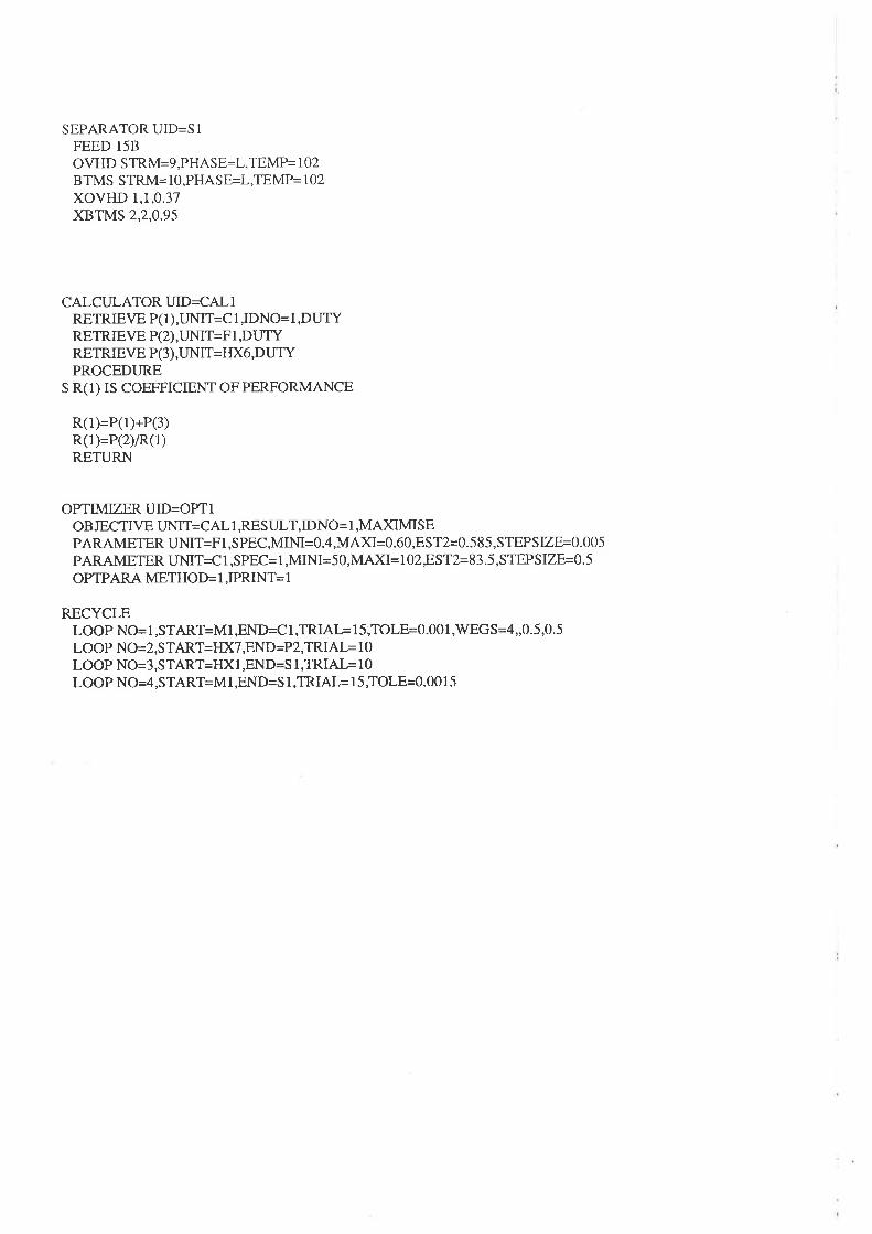
SEPARATOR UID=SlFEED I5BOVHD STRM=9,PHASE=L,TEMP= 1 02BTMS STRM= I0,PHASE=L,TEMP= 1 02xovHD I,1,0.37XBTMS 2,2,0.95
CALCULATOR I-IID=CALIRETRIEVE P( I ),UNIT=C 1,IDNO= l,DUTYRETRIEVE P(2),UNIT=F I,DUTYRETRIEVE P(3),UNIT=FÐ(6,D UTYPROCEDURE
$ R(1) IS COEFFICIENT OFPERFORMANCE
R(1)=P(1)+P(3)R(1)=P(2)/R(1)RETURN
OPTIMIZER UID=OPTIOB JECTIVE I-INIT=CAL 1 ßES ULT, ID NO= I,MAXIMIS EPARAMETER UNIT=FI,SPEC,MIM=O.4,MAXI=0.60,EST2=0.585,STEPSIZE=O.005PARAMETER UNIT=C 1,SPEC= 1,MINI=50,MÆKI=1 02,EST2=83.5,STEPSIZE=O.5OPTPARA METHOD= l,IPRINT= I
RECYCLELOOP NO= l,START=MI,END=C l,TRIAI- l5;TOLE=0.001,IüEGS=4,,0.5,0.5LOOP NO=2,S TAITT=!Ð(7,END=P2,TRIAI= I 0LOOP NO-3,START=IÐ(1,END=S l,TRI AT - 1 0LOOP NO=4,START=M1,END=S l,TRIAL= 15,TOLE=0.0015

UNIT I, Ml SOLVEDUNIT 2, FIX5, SOLVEDLTNIT 3, FI , SOLVEDUNIT 4, Pl SOLVEDUNIT 5, Cl , SOLVED
LOOP 1 SOLVEDAFTER sTRIALSSTRM: 31 T= 58.9 P= 1100.0 RATE= 573.9 DTEMP= 0.00 DCOMP= 0.0003
UNIT 6, TÐ(7 , SOLVEDLINIT 7, F2 , SOLVEDUNIT 8, TÐ(4, SOLVEDL]NIT 9, P2 , SOLVED
LOOP 2 SOLVED AFTER 1 TRIALSSTRM: 7 T= 30.2P= 3500.0 q,{TÞ 8697. DTEMP= 0.00 DCOMP= 0.0000
CONTROLLERUNTT 10, CON2, AT ITERATION 1
SPECIFICATION VALUE = 0.30000E+02, CALC = 0-299888+02PARAMETER CURRENT = 0.82880E+04, NEXT = 0.82880E+M
UNIT IO, CON2, SOLVEDUNIT 11, HXl , SOLVEDI-INIT 12, HX6, SOLVEDUNIT 13, 51 , SOLVED
LOOP 3 SOLVEDAFTER 1TRIALSSTRM: 9 T= 102.0 P= 3500.0 RATE= 53.86 D'IEMP= 0.00 DCOMP= 0.0000
LOOP 4 SOLVEDAFTER 6TRIALSSTRM:94 T= 15.2P= 3500.0RATE=53.86 DTEMP= 0.00DCOMP= 0'0000
STRM: l0 T= 102.0 P= 3500.0 RATE= 8643. DTEMP= 0.00 DCOMP= 0.0000
I.'NIT 14, CALI, SOLVED
'.* AIìTER 3 CYCLES** COI.IVERGENCE METHOD 1 - SECOND ESTIMATE(S) LIMITING -** BETTER SECOND ESTIMATE(S) MAY IMPROVE RESULTS.
OPTIMIZATION HISTORYCYCLE T 2 3
PARA 1 5.8000E-01 5.8500E-01 5.8500E-01PARA 2 8.3000E+01 8.3000E+01 8.3500E+01oBJ. 2.5083E-01 2.5083E-01 2.5080E-01UMT 15, OPTI, SOLVED
VERSION 0484 SMSIMULATION SCIENCES,INC. PROCESSPROJECT MDEAM REFzuGPROBLEM SOLUTION 8-7-90
PAGE 4
'.*{,r, PROBLEM SOLUTION REACHED *.t<*(*

VERSION 0484 SMSIMULATION SCIENCES,INC. PROCESS
PROJECT MDEAM REFRIGPROBLEM SOLUTION 8-7-90
PAGE 5
SUMMARY OF FLASH DRUMS,MI)GR/SPLITTERS AND VALVES
UNIT IDSEQ NONAMETYPE
FEEDS
PRODUCTS
TEMP, DEG CPRESSURE, MMHGFRACTIONLIQUIDDUTY, MM KJ Æ{R
MD(ER9A31
1 (M) s (v)6 (I-)
M1 F21
FLASH
F1
3
2
1
58.94661100.00000.076230.00000
10.0000236.M210.348967.10451
FLASH5
i1
t2 (M)
31.911r236.04270.961160.00000
SUMMARY OF T{EAT EXCHANGE UMTS2 TINIT HX5 , ,IS A HEAT EXCHANGER
*** OPFRATING CONDITIONSDUTY, MM KI /I{R 16.80980
LMTD, DEG C 19.593
FFACTOR I.OOOOO
MTD, DEGC 19.593u * A, KJ /HR DEG C 51950.438
{.'C*' HOT SIDE CONDITIONS INLETFEED(S) 1
LIQLIIDPRODUCTVAPOR, KG MOLS/FIR 519.9301M KGS/HR 38.6136CP, KJ /KG - DEG C 1.1066LrQUrD, KG MOLS/HR 47.8534
M KGS/HR 1.6901
CP, KJ /KG - DEG C 2.9901TOTAL, KG MOLS/Ifi. 621.1835CONDENS(VAPORZ)ATION, KG MOLS/I{RTEMPERATURE, DEG C 58.941PRESSURE, MMHG IIOO.OOO{<** COLD SIDE CONDITIONS INLET
COOLING WATER, KGÆIR 802987.188TEMPERATURE, DEG C 2O.OO
OUTLET
20.00000.00000.0000621.183540.30312.4322621.1835579.930t30.0001100.000OUTLET
802987.18825.000

VERSION 0484 SMSIMULATION SCIENCES,INC. PROCESS
PROJECT MDEAM REFRIGPROBLEM SOLUTION 8-7-90
6 UNIT HX7 , ,IS A HEAT EXCHANGER*{<+, OPERATING CONDITIONSDUTY, MM KJ IHR 30.58462LMTD, DEG C 8.4]6FFACTOR 1.00000
MTD, DEGC 8.4'16
u * A, KJ /HR DEG C 3608280.250
PAGE 7
*T.*. HOT SIDE CONDITIONS INLETFEED(S) 17
LIQTnDPRODUCTVAPOR, KG MOLS/HR O.OOOO
M KGS/I{R 0.0000CP,KJ lKG - DEGC 0.0000LIQUID, KG MOLS/HR 8288.0313M KGSÆ{R 152-2455
CP, KJ IKG - DEG C 4.1505TOTAL, KGMOLSÆIR 8288.0313CoNDENS (VAPORIZ)ATION, KG MOLSÆ{RTEMPERATIIRE, DEG C 83.500PRESSURE, MMHG IIOO.OOO
*** COLD SIDE CONDITIONS INLETFEED(S) 7
LIQUID PRODUCTVAPOR, KG MOLS/HR O.OOOO
M KGSÆ{R O.OOOO
CP, KJ /KG - DEG C O.OOOO
LIQLTID, KG MOLS/HR 8696.7061M KGS/HR 181.5915
CP, KI IKG - DEG C 3.8453TOTAL, KG MOLS/HR 8696.1061CoNDENS (VAPORZ)ATION, KG MOLS/HRTEMPERATURE, DEG C 30.114PRESSURE, MMHG 35OO.OOO
OUTLET
OUTLET
ll0.00000.00000.00008288.0313r52.24554.13098288.03130.000035.1741100.000
15
0.00000.00000.00008696.106r181.59153.85258696.70610.000010.22r3500.000

8 UNIT HX4 , ,IS A HEAT EXCHANGER*,'.* OPERATING CONDITIONSDI.]TY, MMKJ Æ{R 18.939IILMTD, DEG C 11.390
FFACTOR I.OOOOO
MTD, DEGC 11.390
u * A, KJ /HR DEG C 1662783.125
**.{. HOT SIDECONDITONS INLETFEED(S) 12
LIQUIDPRODUCTVAPOR, KG MOLS/HR 332.5951M KGSÆR 20.5528CP, KJ /KG - DEG C 1.7560LTQUID, KG MOLS/HR [email protected] KGS/HR 161.0399
CP, KJ /I(G - DEG C 4.0215TOTAL, KG MOLS/HR 8696.]4T2CONDENS(VAPORIZ)ATION, KG MOLSÆ{RTEMPERATURE, DEG C 31.917PRESSURE, MMHG 236.M3
*** COLD SIDE CONDITIONS INLETCOOLINGWATER, KG/I{R 9M'7O2.OOO
TEMPERATURE, DEG C 2O.OOO
**i, HOT SIDE CONDITTONS INLETFEED(S) 9
LIQUID PRODUCTVAPOR, KG MOLSÆIR O.OOOO
M KGSÆR 0.0000cP, KJ /KG - DEG C o.oo00LTQLTID, KG MOLS/HR 53.862rM KGSÆ{R 2.0689cP, KJ /KG - DEG C 2.9017TOTAL, KGMOLSÆIR 53.8621CONDENS(VAPORZ)ATION, KG MOLSÆ{RTEMPERATURE, DEG C 1O2.OOO
PRESSURE, MMHG 35OO.OOO
OUTLET
1I UNIT HXl , , IS A I{EAT EXCHANGER*** OPERATING CONDITIONSDUTY, MM KI Æ{R 0.21926LMTD, DEG C 14.394FFACTOR I.OOOOO
MTD, DEGC 14.394u * A, KJ /HR DEG C 15232.754
r30.00000.00000.00008696;14r2181.59283.84558696.74r2332.595729.988236.M3
9A0.00000.00000.000053.862r2.06892.893r5386210.000075.2213500.000
OUTLET904702.N025.000
OUTLET

*',{< COLD SIDE CONDITIONS INLETFEED(S) 15
LIQUID PRODUCTVAPOR, KG MOLSÆ{R O.OOOO
M KGS/HR O.OOOO
CP,zu KG - DEGC O.OOOO
LIQUID, KG MOLS/HR 8696.7061M KGS/HR I8I.5915CP, KJ /I(G - DEG C 3.8525TOTAL, KG MOLS/FIR 8696.7061CONDENS (VAPORIZ)ATION, KG MOLSÆ{RTEMPERATURE, DEG C 10.221
PRESSURE, MMHG 35OO.OOO
*** HOT SIDE CONDITIONS INLETSTEAM, KG/IIR IO&2.438SATURATION PRESSURE, MMHGSATURATION TEMPERATURE, DEG C
*T,* COLD SIDE CONDITIONS INLETFEED(S) 15A.
LIQUIDPRODUCT 158VAPOR, KG MOLSÆ{R O.OOOO
M KGS/HR O.OOOO
CP, KJ /KG - DEG C O.OOOO
LrQUrD, KG MOLSÆ{R 8696.106rM KGSÆ{R 181.5915CP, KJ iKG - DEG C 3.852'ITOTAL, KG MOLS/HR 8696.7067CoNDENS (VAPORIZ)ATION, KG MOLS/IR.TEMPERATURE, DEG C ]0.513PRESSI.TRE, MMHG 35OO.OOO
i5A0.00000.00000.00008696.106r181.59153.85278696.70610.000070.5133500.000
OUTLET
OUTLETr0&2.4381478.249120.000
OUTLET
12 UNIT HX6 , ,IS A I{EAT EXCHANGER*** OPERATING CONDITIONSDUTY, MM zu /HR 2342941LMTD, DEG C 31,134FFACTOR I.OOOOO
MTD, DEG C 31,134u * A, KJ /I{R DEG C 752533.188
0.00000.00000.00008696.7061181.59153.81928696.70610.0000102.0003500.000

VERSION 0484 SMSIMULATION SCIENCES,INC. PROCESS
PROJECT MDEAM REFRIGPROBLEM SOLUTION 8-7-90
PAGE 1I
SUMMARY OF COMPRESSOR/ÐPANDER/PUMP/TURBINE UNITS4 UNIT Pl , , IS A PUMP
*¡I<i< FEED STREAMS ARE 6"i.'T LIQUID PRODUCT IS STREAM 26**'. OPERATING CONDITIONS
woRK, KW 3.04
EFFICIENCY, PERCENT 60.00
MOLE FRACTION LIQUIDTEMPERATURE, DEGCPRESSURE, MMHGTIEAD, MHOTVOLUME, M3/HR
9 UNITP2 , ,IS APUMP*** FEED STREAMS ARE 13*!** LIQUID PRODUCT IS STREAM 7**,r. opFRTA,TING CONDITIONS
WORK, KWEFFICIENCY, PERCENT
MOLE FRACTION LIQI-IIDTEMPERATURE, DEGCPRESSURE, MMHGHEAD, MHOT VOLUME, M3Æ{R
INLET1.000010.000236.0427
15.081
OUTLET1.000010.1 83
3500.0000101.8107
15.081
40.r960.00
INLET1.000029.988236.0421
r99.433
OUTLET1.000030.1133500.00008r.2321
t99.449

VERSION 0484 SMSIMULATION SCIENCES,INC. PROCESSPROJECT MDEAMREFRIG UNIT 13 - SIPROBLEM SOLUTION 8-7-90
SUMMARY OF COMPONENT SEPARATORS
PAGE 12
UNIT IDSEQ NONAME
FEEDS
PRODUCTSTEMP, DEG CPRESSURE, MMHGFRACTION LIQUIDDUTY, MM KJ /HR
e (L) 10 (L)102.0000 102.0000
3500.0000 3500.00001.00000 1.00000
-0.15790
s113
l5B
UNIT IDsEQ NONAME
R( 1)R( 2)R( 3)R( 4)R( 5)R( 6)R( 7)R( 8)
SUMMARY OF CALCULATOR UNITSREPORT OF RESULTS VECTORS
CALIl4
2.50798F-OtUNDEFINEDUNDEFINEDUNDEFINEDTINDEFINEDUNDEFINEDUNDEFINEDUNDEFINED

VERSION 0484 SMSIMULATION SCIENCES,INC. PROCESS
PROJECT MDEAMREFRIG UNIT 5-ClPROBLEM SOLUTION 8-7-90
PAGE 14
I SUMMARY FOR COLUMN UNIT 5 . Cl ,
I TOTAL NUMBER OF ITERATIONSFASTMETHOD O
SURE METHOD IIl2 COLUMN SUMMARY
TRAY TEMP PRESS NET FLOW RATES, KG MOLS/HR IIEAT(COOL)ERLIQUID VAPOR DUTIES
DEG C MMHG PHASE(I-) PHASE(Ð F'EED PRODUCT MM KJ ÆIR
58.9'1r.6
78.278.618.783.5
PROBLEM
TRAYCOMPONENTI DMEAMI2ll2o-KG MOLSÆ{RTRAYCOMPONENT1 DMEAMI2H20KG MOLSÆIR
I23
45
6
1100.001100.001100.001100.001100.001100.00
225.1190.1r9t.7191.88333.1
580.5544.9546.5546.6
45.r
2r9.tL 573.9V
8&2.8L8288.0L 4.8985
3 FEED AND PRODUCT STREAMS MASS RATES IIEAT RATES* FEED STREAMS: KG MOLS/FIR MM KJ Æ{R
10 TO TRAY 5 IS LIQUID FROM UNIT 13, Sl 0.86428E+04 0.66631E+02
26 TO TRAY I IS LIQUID FROM UNIT 4, Pl 0.219018+03 -0'472158+00* PRODUCT STREAMS:I7 IS LIQUID STREAM FROM TRAY 6 0.82880E+04 0.51509E+02
3l IS VAPOR STREAMFROMTRAY 1 0.57389E+03 0.t95498+02OVERALL MASS BALANCE, (FEEDS - PRODS) 0.00000E+00OVERALL HEAT BALANCE, (IIIN - HOUT) -0.61798E-03
4 SPECIFICATIONVALUESPARAMETER TRAY COMP. SPECIFICATION SPECIFIED CALCLILATED
TYPE NO NO TYPE VALUE VALUETRAY 6 TEMP 0.8350E+02 0.8350E+02
SOLUTION 8-7-90IIA TRAY COMPOSITIONS
1 -------- 2 --------XYXY
0.3167E+00 0.8822E+00 0.1936E-01 0.11628+OO
0.6833E+00 0.1184E+00 0.9806E+00 O.22448+000.2257E+03 0.5739E+03 0.l90lE+03 0.5805E+03
3 -------- 4 --------XYXY
0.1020E-01 0.7024E+00 0.9826E-02 0.6970E+000.9898E+00 0.29798+00 0.9902E+00 0.3032E+000.1917E+03 0.5449E+03 0.19188+03 0.5465E+03

STREAM COMPONENT FLOV/ RATES - KG MOLSÆ{R
STREAMID I 2 5
NAMEPHASE MDGD LIQUID VAPOR
TRAYCOMPONENTl DMEAMIzH20KG MOLSÆ{R
l DMEAMI2H20TOTALSTEMPERATURE, DEG CPRESSURE, MMHGH,MMKJ /I]RMOLE FRACTLIQTIIDRECYCLE CONVERGENCE
STREAM IDNAMEPI{ASEl DMEAMI2f120TOTALSTEMPERATURE, DEG CPRESSURE, MMHGH, MM KJ /I{RMOLE FRACT LIQUIDRECYCLE CONVERGENCE
STREAM IDNAME
PHASEI DMEAMI21120TOTALSTEMPERATURE, DEG CPRESSURE, MMHGH, MM zu /TIRMOLE FRACT LIQUIDRECYCLE CO}N'ERGENCE
5 -------- 6 --------XYXY
0.9804E-02 0.6965E+00 0.64288-02 0.6304E+00
0.99028+00 0.3035E+00 0.9936E+00 0.3696E+00
0.8333E+04 0.5466E+03 0.8288E+04 0.4509E+02
6
LIQLIID
525.91r7101.8119627.183558.94661100.000020.06500.01620.0000
525.9717101.8119627.183530.00001100.00003.25521.00000.0000
398.80829.9025408.710610.0000236.042770.84290.00000.0000
10
LIQUID432.r4748210.702r8@2.8438102.00003500.000066.63131.00000.0000
r2'1.16359r.9094219.072910.0000236.U27-0.48311.00000.0000
7
LIQLIID452.08138244.66028696.74r230.17333500.000012.97301.00000.0000
t2
LIQTIID19.928533.933653.8621102.00003500.00000.73301.00000.0000
l1
LIQLIID53.273r8234.75788288.031335.17351100.000020.92431.00000.0000
9
13
MD(ED452.08138244.66028696.141237 .9r11236.M2131.16140.96180.0000
LIQUID452.08138244.66028696.74t229.9883236.M2112.82831.00000.0000
15
LIQUID452.06998244.63578696.706110.22013500.000043.55181.00000.0000
LIQIJID53.273r8234.75788288.03 13
83.50001100.000051.50891.00000.0000
t7

STREAM COMPONENT FLOW RATES - KG MOLS/HRSTREAM ID 26 31 9A 154
NAMEPHASE LIQUID VAPOR LIQTIID LIQUIDl DMEAMI 127.1.635 505.9881 t9.9285 452.0699
2Í120 gr.gog4 '67.8982 33.9336 8244.6357
TOTALS 219.0129 573.8863 53.8621 8696.706r
TEMPERATURE, DEG C 10.1830 58.8',779 ',75.2207 l0-5r28PRESSURE, MMHG 3500.000 1100.0000 3500.0000 3500.0000
H, MM zu /I{R -0.472r 19.5493 0.5137 43.1710
MOLE FRACTLIQUID 1.000 0.0000 1.0000 1.0000
RECYCLECOI.IVERGENCE 0.0000 0.0003 0.0000 0.0000
STREAMIDNAME
PHASEl DMEAMI2tf20TOTAI.STEMPERATURE, DEG CPRESSURE, MMHGH, MMKJ Æ{RMOLE FRACT LIQUIDR-ECYCLE CO}TVERGENCE
15B
LIQUID452.06998244.63518696.706r102.00003500.000067.20ó/.1.00000.0000

PROCESSft Innut and Outout File Listinss
THE MODIFIED AQUA.AMMONIA REFRIGERATION
CYCLE WITHOUT PRECOOLING
194
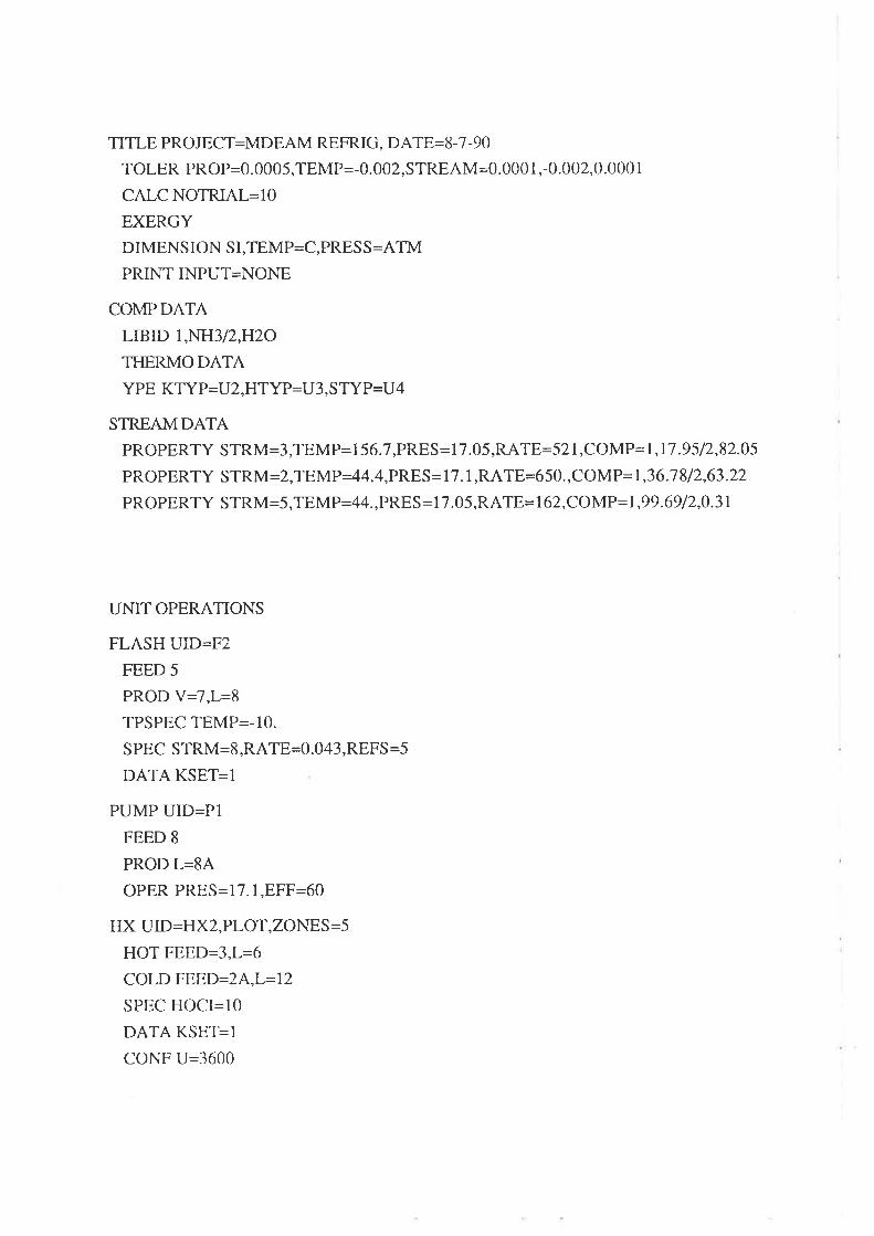
TITLE PROJECT:MDEAM REFRIG, DATE=8-7-90
TOLER PROP:0.0005,TEMP=-0.002,STREAM=0.000 1,-0.002,0.000 1
CALC NOTRIAL=IO
EXERGY
DIMENSION SI,TEMP:C,PRES S =ATMPRINT INPUT=NONE
COMP DATA
LIBID 1,NH3/2,H2O
TFIERMO DATA
YPE KTYP=U2,HTYP=U3,STYP=U4
STREAM DATA
PROPERTY STRM:3,TEMP= 1 56.7,PRES = 1 7. 05,RATE =52L,COMP= 1, 17 .9 5 12,82.05
PR OP ERTY S TRM = 2,'f Ell{P -44. 4, PRES = 1 7 . 1, RATE =6 5 0., C OM P = 1,3 6 .7 8 / 2,63 .22
PROPERTY STRM=5,TEM P=44.,PRES = 1 7. 05,RATE= 1 62,COMP :1,99.69 12,0.31
UNIT OPERATIONS
FLASH UID=F2
FEED 5
PROD V=7,L=8
TPSPEC TEMP=-10.
S PEC STRM=8,RATE=0.043,REFS=5
DATA KSET=I
PUMP UID=PI
FEED 8
PROD L=84
OPER PRES=17.1,8FF:60
HX UID=HX2,PLOT,ZONES =5
HOT FEED=3,L=6
COLD FEED=24,L:72
SPEC HOCI=10
DATA KSET=I
CONF U=3600

MIXER UID=M2
FEED 6,7
PROD M=15
HX UID=HX4
HOT FEED:15,L=1 1,DP=O. 12
SPEC HOT,LFRACT=1.0
UTILIY WATER,TIN=27,TOUT=40
DATA KSET:ICONF U:3600
PUMP UID=P2
FEED 11
PROD tF2OPER PRES=17.1,EFF=60
MIXER UID=MIFEED 2,84
PROD M=24
CONTROL UID=CON2
SPEC STRM=I 1,TEMP=44.0
PARAM STRM:3,MAXI=3000,MINI= I 00,EST2=2500
COLUMN UID:COLIPARA TRAY=7,FAST:5,SURE=30
FEED I2,4
PRODUCT OVHD=5,BTMS=3, I 662
PSPEC TOP=17.1
CONDENSER TYPE=3
HEAT r,7,5.30/2,1,-3.56
PRINT TRAY:IO
S PEC TRAY=7,TEMP= 1 54.00
SPEC TRAY= l,PHASE=L,RATE=70
VARIABLE HEAT=l,2
TEM p 1,44.0 /2,6 5.6 I 3,99 .8 I 4,r0 5 ;7 I 5,107 .6 I 6,1 rl .8 /1,1 49 .1
vApouR t,r47 .612,t80.8/3, 161.314,158.9 l5 J55.7 16,r53/1,145.1
LIQUID 1,33. /2,r3.6 13,l 1 .3 / 4,51 8.3 I 5,51 5.1 I 6,5 67 .8 /1,422.1
DATA KSET=I
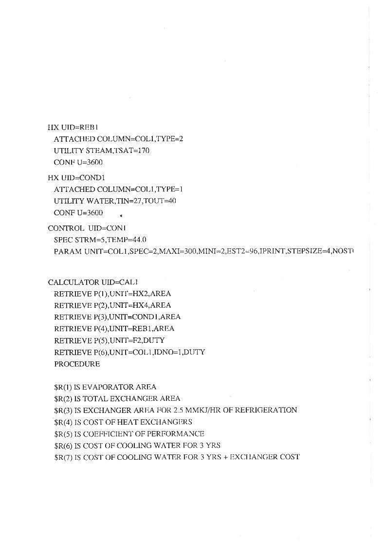
HX UID=REB1
ATIACHED COLUMN=COL l,TYPE=2
UTILITY STEAM,TSAT= 1 70
CONF U=3600
HX UID=CONDI
ATTACHED COLUMN=COL I,TYPE= 1
UTILITY V/ATER,TIN=27,TOUT=40
CONF U=3600 ¡
CONTROL UID=CONI
SPEC STRM=5,TEMP=44.0
PARAM UNIT=COLl,SPEC=2,MAXI=300,MINI:2,EST2=96,IPRINT,STEPSIZE-4,NOSTI
CALCULATOR UID=CALI
RETRIEVE P( 1 ),UNTI=HX2,AREARETRIEVE P(2),UNTI:HX4, AREA
RETRIEVE P(3),UNTT=COND 1,AREA
RETRIEVE P(4),UMT=REB I,AREA
RETRIEVE P(5),UNTT=F2,DUTY
RETzuEVE P(6),UNTI=COL1,IDNO= I,DUTY
PROCEDURE
$R(1) IS EVAPORATOR AREA
$R(2) IS TOTAL EXCHANGER AREA
$R(3) IS EXCHANGER AREA FOR 2.5 MMKJ/FIR OF REFRIGERATON
$R(4) rS COST OF HEAT EXCHANGERS
$R(5) rS COEFFICIENT OF PERFORMANCE
$R(6) rS COST OF COOLING WATER FOR 3 YRS
$R(7) IS COST OF COOLING WATER FOR 3 YRS + EXCHANGER COST

R(1)=P15;70.036
R(2)=R(1)+P(1)
R(2)=B12¡+P(2)
R(2)=B12;+P(3)
R(2)=P12;+P(a)
R(3)=R(2)/P(s)
R(3)=R(3)*45.36
R(4)=R13¡*556
R(4)=R(4)+78500
R(5)=P(5)/P(6)
R(6)=P(s)+P(6)
R(6)=R(6)Æ(5)
R(6)=P16;*45.36
R(6)=R(6)*22500
R(7)=P14¡+R(6)
RETURN
OFT|IMIZER UID=OPT
OB JECTIVE UNIT=CAL 1, RES ULT,IDNO=T,MINIMIS E
PARAMETER UNIT:F2,S PEC,MINI=0. 02,MAXI=O. 1 3,EST2=0.04 l,STEPS IZE=O.002
PARAMETER UMT=HX2,S PEC,MIM=4,MAXI:50,ES T2=9,STEPS IZE= 1
PARAMETER UNIT=COL l,SPEC=1,MIM=105,MAXI= I 60,EST2= 1 55,STEPSIZE=I
OPTPARA METHOD= I,IPRINT= 1
RECYCLE
LOOP NO= I,START=HX2,END=M I
LOOP NO=2,START=F2,END=CON 1,TRIAL:25

UNIT 1,F2, SOLVED
UNIT z.PI SOLVED
UNIT 3,HX2, SOLVED
UNIT 4,M2 , SOLVED
UNIT 5,HX4, SOLVED
UNIT 6,P2, SOLVED
UNIT 7, M1 , SOLVED
LOOP 1 SOLVED AFTER l TRIALS
STRM:24 T= 44.6P= 17.1RATE=662.5 DTEMP= 0.00DCOMP= 0.0000
UNTT 8, CON2, SOLVED
UNTI 9, COLI, SOLVED
CONTROLLER UNIT 12, CONI, AT ITERATION 1
SPECIFICATION VALUE = 0.440008+02, CALC = 0.440028+02
PARAMETER CURRENT = 0.625878+02, NEXT = 0.625878+02
IJNTI 12, CONl, SOLVED
LOOP 2 SOLVED AFTER 5 TRIALS
STRM: 3 T= 157.0 P= 17.1 RATE= 500.6 DTEMP= 0.00 DCOMP= 0.0000
STRM:5 T= 44.0P= 17.1 RATE= 161.9 DTEMP= 0.00 DCOMP= 0.0000
UNTT 10, REB 1, SOLVED
UNTI 11, COND, SOLVED
UNTT 13, CALI, SOLVED
*>K AFIER 10 CYCLES
** CONVERGENCE METHOD 1 - OBJECTryE FUNCTION NO LONGER IMPROVES.
OPTIMTZATION HISTORY
CYCLEI2345PARA 1 4.3000E-02 4.10008-02 4.1000E-02 4.1000E-02 4.04268-02
PARA 2 1.0000E+01 1.00008+01 9.00008+00 9.0000E+00 8.9144E+00
PARA 3 1.54008+02 1.54008+02 1.54008+02 1.5500E+02 1.5595E+02
OBJ. 6.4509E+06 6.43908+06 6.43548+06 6.3958E+06 6.3618E+06
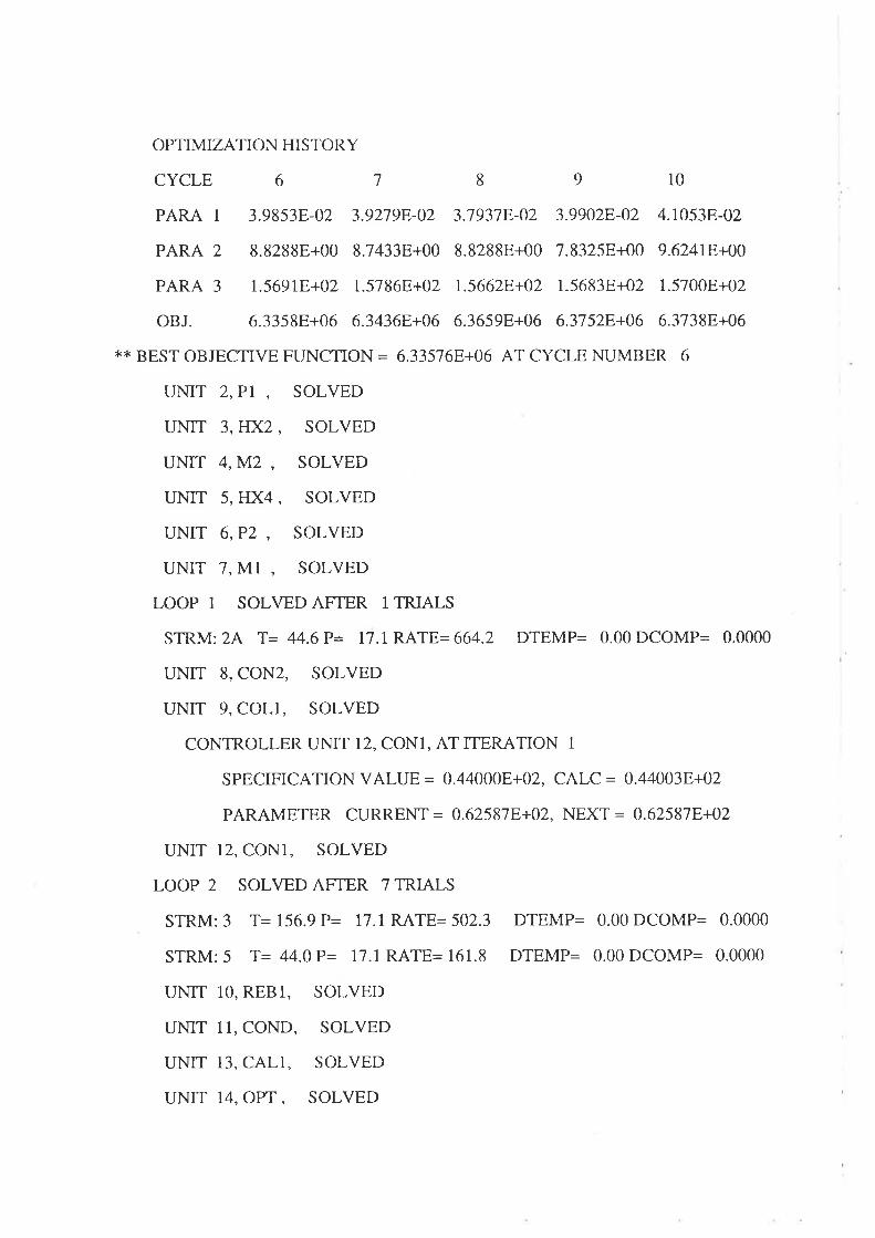
OPTIMIZATION HISTORY
CYCLE618910PARA 1 3.9853E-02 3.92798-02 3.t9318-02 3.99028-02 4.1053E-02
PARA 2 8.8288E+00 8.74338+00 8.8288E+00 7.8325E+00 9.62418+00
PARA 3 l.569IE+02 1.5786E+02 I.56628+02 1.5683E+02 1.5700E+02
OBJ. 6.3358E+06 6.34368+06 6.3659E+06 6.37528+06 6.3738E+06
x* BEST OBJECTIVE FUNCTION = 6.335168+06 AT CYCLE NUMBER 6
UNIT 2,PI , SOLVED
UNIT 3,HXZ, SOLVED
UNIT 4,M2 , SOLVED
UNIT 5, HX4 , SOLVED
UNIT 6,P2 , SOLVED
UNIT 7, Ml , SOLVED
LOOP 1 SOLVED AFTER l TRIALS
STRM:24 T= 44.6P= l7.1RATE=664.2 DTEMP= 0.00DCOMP= 0.0000
UNIT 8, CON2, SOLVED
UNIT 9, COLI, SOLVED
CONTROLLER UNIT 12, CONI, AT ITERATION 1
SPECIFICATION VALUE = 0.440008+02, CALC = 0.440038+02
PARAMETER CURRENT = 0.625818+02, NEXT = 0.625878+02
UNTT 12, CONI, SOLVED
LOOP 2 SOLVED AFTER 7 TRIALS
STRM: 3 T= 156.9 P= 17.1 RATE= 502.3 DTEMP= 0.00 DCOMP= 0.0000
STRM: 5 T= 44.0P= 17.1 RATE= 161.8 DTEMP= 0.00 DCOMP= 0.0000
UNTI 10, REBl, SOLVED
UNIT 1I, COND, SOLVED
UNIT 13, CALI, SOLVED
UNIT 14, OFT| , SOLVED

VERSION 0484 SM
SIMULATION SCIENCES, INC. PROCESS
PROJECT MDEAM REFRIG
PROBLEM SOLUTION 8-7-90
PAGE 4
**** PROBLEM SOLUTION REACHED ***x
SUMMARY OF FLASH DRUMS,MIXER/SPLITTERS AND VALVES
UNTI ID
EQ NO
NAME
TYPE
FEEDS
FLASH
5
MD(ER
6
7
1s (M)
68.2266
2.8055
0.82309
0.00000
MIXER
2
8A
2A (L)
44.5615
17.1000
1.00000
0.00000
M1
1
lvI2
4
F2
I
PRODUCTS 7 (V)
8 (L)
TEMP, DEG C -1O.OOOO
PRESS, ATM 2.8055
FRACT LTQUTD 0.03985
DUTY, MM KJ lHR 2.]2]02

SUMMARY OF HEAT E,XCHANGE UNITS
3 UNIT HX2 , , IS A HEAT EXCHANGER*** OPERATTNG CONDITIONS
DUTY, MM KJ /FIR 4.09450
WEIGHTED LMTD, DEG C 19.654
F FACTOR I.OOOOO
MTD, DEGC 19.654
U * A, KJ ÆIR DEG C 208326.109
u, KJ /HR DEG C SQ M 3600.000
A, SQ M 57.868
,K'<* HOT SIDE CONDITIONS INLET
FEED(S) 3
LIQUID PRODUCT
VAPOR, KG MOLS/FIR O.OOOO
M KGSÆIR O.OOO5
CP, KJ Æ(G - DEG C 2.6914
LIQUID, KG MOLS/FIR 502.3283
M KGS/HR 8.9604
CP, KJ /KG - DEG C 4.6546
TOTAL, KG MOLS/HR 502.3283
CONDENS(VAPORTZ)ATION, KG MOLS/FIR
TEMPERATURE, DEG C 156.908
PRESSURE, ATM 17.100
*** COLD SIDE CONDMONS INLET
FEED(S) 2A
MD(ED PRODUCT
VAPOR, KG MOLS/FIR O.OOOO
M KGS/HR O.OOOO
CP, KJ /I(G - DEG C O.OOOO
LIQUID, KG MOLS/HR 664.1602
M KGS/FIR II.7I]2CP, KJ Æ(G - DEG C 4.4855
TOTAL, KG MOLS/FIR 664.1602
CONDENS(VAPORTZ)ATION, KG MOLS/FIR
TEMPERATURE, DEG C 44.562
PRESSURE, ATM 17.100
OUTLET
6
0.0000
0.0000
0.0000
502.3283
8.9609
4.3161
s02.3283
0.0000
53.391
17.100
OI.]TLET
l2r5.4922
0.2648
2.7243
648.6680
rr.45234.7239
664.1602
75.4922
r14.607
17.100

5 UNIT HX4 , , IS A HEAT EXCHANGER
*** OPERATING CONDMONS
DUTY, MM KJ ÆIR
LMTD, DEG C
F FACTOR
MTD , DEG C
U*A,KJ ÆIR DEGC
U, KJ /HR DEG C SQ M
A, SQM
**,F COLD SIDE CONDITIONS
COOLING WATER, KG /HR
TEMPERATURE, DEG C
'<** HOT SIDE CONDITIONS INLET
FEED(S) 15
LIQUID PRODUCT
VAPOR, KG MOLS/ÉIR 116.356
M KGSÆ{R 1.9899
CP, KJ IKG - DEG C 2.2962
LIQUID, KG MOLSÆIR 541.3550
M KGSÆIR 9.6113
CP,zuA(G -DEGC 4.3809
TOTAL, KG MOLSÆIR 657 .1112
CONDENS (VAPORIZ)ATION, KG MOLS/HR
TEMPERATURE, DEG C 68.22]
PRESSURE, ATM 2.805
4.4687 5
22.13r
1.00000
22.r3r201927.315
3600.000
56.089
INLET
82102.953
27.000
OUTLET
11
0.0000
0.0000
0.0000
657.1rr2
rr.6012
4.4904
657 .t 172
tt6.3562
43.984
2.685
OUTLET
82102.953
40.000

10 UNIT REB1, ,IS A HEAT EXCHANGER
'K** OPERJATING CONDMONS
DUTY, MM KJ ÆIR
LMTD, DEG C
F FACTOR
MTD, DEG C
U*A,KJ /HR DEGC
U, KJ /HR DEG C SQ M
A, SQM
5.94961
24.952
1.00000
24.952
238443.094
3600.000
66.234
*** HOT SIDE CONDITIONS INLET
STEAM, KG ÆIR 2830.137
SATURATION PRESSURE, ATM
SATURATION TEMPERATURE, DEG C
*X* COLD SIDE CONDITIONS INLET
STREAM IS FROM COLUMN COLI, UNIT 9
VAPOR, KG MOLSÆIR O.OOOO
M KGSÆIR O.OOOO
CP, KJ /KG - DEG C O.OOOO
LIQUID, KG MOLSÆIR 660.4044
M KGS/FIR 11.6987
CP, KJ Æ(G - DEG C 4.1049
TOTAL, KG MOLS/FIR 660.4044
CONDENS(VAPORTZ)ATION, KG MOLSÆIR
TEMPERATURE, DEG C 12].592
PRESSURE, ATM 17.100
OUTLET
2830.t37
1.780
170.000
OUTLET
158.0592
2.7376
2.6913
502.3452
8.9612
4.6546
660.4044
158.0592
156.896
I 7. 100

11 UNIT COND, , IS A HEAT EXCHANGER
*** OPERATING CONDITIONS
DUTY, MM zu /FIR
LMTD, DEG C
F FACTOR
MTD, DEG C
U*A,KJ /HR DEGC
U, KJ /HR DEG C SQ M
A, SQM
*** COLD SIDE CONDITIONS
COOLING WATER, KG /FIR
TEMPERATURE, DEG C
',** HOT SIDE CONDITIONS INLET
STREAM IS FROM COLUMN COLI, UNIT 9
VAPOR, KG MOLS/FIR 2243906
M KGS/FIR 3.82T8
CP, KJ Æ(G - DEG C 3.1813
LIQUID, KG MOLS/FIR 0.0000
M KGSÆIR O.OOOO
CP, KJ /I(G - DEG C O.OOOO
TOTAL, KG MOLSÆIR 224.3906
CONDENS(VAPORIZ)ATION, KG MOLS/FIR
TEMPERATURE, DEG C 52.236
PRESSURE, ATM 17.100
4.24328
14.47 7
1.00000
14.417
293219.938
3600.000
81.450
INLET
11960.492
27.000
OUTLET
0.0000
0.0000
0.0000
224.3906
3.8218
5.0297
224.3906
224.3906
43.964
17.100
OUTLET
71960.492
40.000

SUMMARY OF COMPRESSORÆXPANDERÆUMPÆURBINE UNITS
2 UNIT Pl , IS A PUMP**<'K FEED STREAMS ARE 8
X*:K LIQUID PRODUCT IS STREAM 8A*** OPERATING CONDMONS
woRK, KW 0.l lEFFICIENCY, PERCENT 60.00
MOLE FRACTION LIQUID
TEMPERATURE, DEG C
PRESSURE, ATM
HEAD, M
HOT VOLUME, M3ÆIR
6 UNIT P2 , , IS A PUMP{,r<* FEED STREAMS ARE 11
,K** LIQUID PRODUCT IS STREAM 2
X**< OPERATNG CONDITIONS
WORK, KW
EFFICIENCY, PERCENT
MOLE FRACTION LIQUID
TEMPERATURE, DEG C
PRESSURE, ATM
HEAD, M
HOT VOLUME, M3/FIR
TNLET
1.0000
-10.000
2.8055
0.167
OUTLET
1.0000
-9.415
17.1000
314.9895
0.168
9.92
60.00
INLET
r.0000
43.984
2.6855
14.610
OUTLET
1.0000
44.410
17.1000
3r3.7579
t4.610

UNIT ID
SEQ NO
NAME
R( 1)
R( 2)
R( 3)
R( 4)
R( s)
R( 6)
R( 7)
R( 8)
SUMMARY OF CALCULATOR UNITS
REPORT OF RESULTS VECTORS
CALl13
7.515078+01
3.327628+02
5.53500E+03
3.122758+06
4.583538-01
3.241278+06
6.370028+06
UNDEFINED
T SUMMARY FOR COLUMN UNIT 9. COLI,
1 TOTAL NUMBER OF ITERATIONS
FAST METHOD O
SURE METHOD 770
2 COLUMN SUMMARY
TRAY TEMP PRESS NET FLOW RATES, KG MOLSÆIR
VAPOR
PHASE(v)
224.4
r92.4
182.8
r66.6
t64.0
HEAT(COOL)ER
DUTIES
DEG C
| 44.0
2 52.2
3 98.8
4 1t4.6
5 117.0
6 127.6
7 t56.9
ATM
17.10
17.10
17.10
t7.r017.10
17.10
fl.r0
LIQUID
PHASE(L)
62.6
30.6
2t.0
668.9
666.3
660.4
158.1
FEED
664.2M
PRODUCT MM KJ ÆIR
161.8L -4.2433
s02.3L 5.9496

3 FEED AND PRODUCT STREAMS MASS RATES HEAT RATESX FE,ED STREAMS: KG MOLS/HR MM KJ /FIR
12 TO TRAY 4IS MIXED FROM UNIT 3,fjXZ 0.66416E+03 0.35989E+01X PRODUCT STREAMS:
3 IS LIQUID STREAM FROM TRAY 7 0.50233E+03 0.472438+01
5 IS LIQUID STREAM FROM TRAY 1 0.16183E+03 0.58013E+00
OVERALL MASS BALANCE, (FEEDS - PRODS) 0.00000E+00
OVERALL HEAT BALANCE, (HIN - HOUT) 0.761518-03
4 SPECIFICATION VALUES
PARAMETER TRAY COMP. SPECIFICATION SPECIF'IED CALCULATED
TYPE NO NO TYPE VALUE VALUE
TRAY 7 TEMP 0.1569E+03 0.15698+03
TRAY LIQD 1 ML RATE 0.62598+02 0.62598+02
IIA TRAY COMPOSITIONS
TRAY
COMPONENT
I NH3
2fl20KG MOLS/FIR
TRAY
COMPONENT
1 NH3
2Hzo-
KG MOLS/FIR
TRAY
COMPONENT
1 NH3
2H20KG MOLS/ÉIR
X
0.99918+00
0.85028-03
0.62598+02
Y
0.99918+00
0.85028-03
0.161 8E+03
2
X
0.81108+00
0.18908+00
0.3058E+02
Y
0.9990E+00
0.85018-03
0.22448+03
1
J
X
0.44408+00
0.5560E+00
0.20968+02
Y
0.9689E+00
0.3076E-01
0.19248+03
4
X
0.36588+00
0.63428+00
0.66898+03
Y
0.93558+00
0.6454E-01
0.1 828E+03
5
X
0.3543E+00
0.6457E+00
0.66638+03
Y
0.9284E+00
0.71588-01
0.1 666E+03
6
X
0.30538+00
0.69478+00
0.6604E+03
Y
0.8905E+00
0.1095E+00
0.16408+03

TRAY
COMPONENT
1 NH3
2H20KG MOLS/FIR
7
X0.17928+00
0.8208E+00
0.5023E+03
Y
0.7059E+00
0.29428+00
0.158 1E+03
STREAM COMPONENT FLOW RATES - KG MOLS/FIR
STREAM ID
PHASE
1 NH3
2Hzo.
TOTALS
TEMPERATURE, DEG C
PRESSURE, ATM
H, MM KJ ÆIR
MOLE FRACT LIQUID
RECYCLE COI.IVERGENCE
STREAM ID
PHASE
1 NH3
2Hzo.
TOTALS
TEMPERATURE, DEG C
PRESSURE, ATM
H, MM KJ /TÌR
MOLE FRACT LIQUID
RECYCLE CONVERGENCE
2
LIQUID
245.394r
4t2.3110
657.7tt2
44.4t03
17.1000
-0.4892
1.0000
0.0000
lVAPOR
t55.3822
0.0007
r55.3829
-10.0000
2.8055
3.3140
0.0000
0.0000
J
LIQUID
90.0117
412.3r66
502.3284
1s6.9083
17.1000
4.7243
1.0000
0.0000
8
LIQUID
6.372r
0.1369
6.4490
-10.0000
2.8055
-0.0069
1.0000
0.0000
5
LIQUID
16r.6943
0.r376
161.8319
44.0035
17.1000
0.5801
1.0000
0.0000
11
LIQUID
245.394r
4t2.3r70
657 .17r243.9835
2.6855
-0.5249
1.0000
0.0000
6
LIQUID
90.0119
4r2.3164
502.3283
53.3908
17.1000
0.6298
1.0000
0.0000
t2
MD(ED
25r.7040
4t2.4562
664.1602
rr4.6066
17.1000
3.s989
0.9767
0.0000

STREAM ID
PHASE
1 NH3
2H}o-
TOTALS
TEMPERATURE, DEG C
PRESSURE, ATM
H, MM KJ /HR
MOLE FRACT LIQUID
RECYCLE CONVERGENCE
l5
MIXED
245.394r
4r2.3r70
657.7rtz
68.2266
2.8055
3.9439
0.8231
0.0000
2A
LIQUID
251.7062
412.4539
664.1602
44.5615
17.1000
-0.4956
1.0000
0.0000
8A
LIQUID
6.3r2r
0.1369
6.4490
-9.4r54
I 7.1000
-0.0065
1.0000
0.0000
STREAM AVAILABILITY TABLE
TZERO: 15.00 DEG C
IDNAMERATEENTHALPYENTROPYB=(H-TOS)KG MOLSÆIR MM KJ /HR MM KJ /HR K MM KJ /HR
2
3
5
6
7
8
11
I2
15
2A
8A
6.5718+02
5.0238+02
1.618E+02
5.0238+02
1.5548+02
6.4498+00
6.5178+02
6.6428+02
6.577F+02
6.6428+02
6.4498+00
-4.8928-0r
4.1248+00
5.8018-01
6.298E-01
3.314E+00
-6.8568-03
-5.2498-01
3.599E+00
3.944E+00
-4.956E-01
-6.451E-03
2.1088-03
r.556E-02
1.9808-03
4.4928-03
r.2848-02
-2.2318-05
2.055E-03
1.3968-02
r.6968-02
2.111E-03
-2.168E-05
-1.097E+00
2.4168-01
9.7368-03
-6.6448-0r
-3.850E-01
-4.2118-04
-1.1178+00
-4.2318-01
-9.437E-0r
-1.104E+00
-2.0298-04

UNIT AVAILABILITY B ALANCE
UID NAME DELTA-B W-EXT DT/TY
MM KJ /FIR
F2
P1
HXz
M2
HX4
P2
M1
COLl
3.9518-01
-2.248F-04
2.2528-01
-1.0578-01
r.7348-01
-2.0588-02
1.2038-03
-6.7448-07
0.0008+00
4.043F-04
0.000E+00
0.000E+00
0.0008+00
3.5718-02
0.000E+00
0.000E+00
2.7278+00
0.000E+00
0.0008+00
0.000E+00
4.4698+00
0.0008+00
0.0008+00
5.950E+00
-4.2438+00
5.950E+00
4.2438+00
REBl
COND
0.000E+00
0.000E+00
0.0008+00
0.000E+00

PROCESSru Innut and Output File Listings
CONVENTIONAL AQUA-AMMONIA RBFRIGERATION
CYCLE WITHOUT PRECOOLING
195

TITLE PROJECT=MDEAM REFRIG, DATE=8-7-90
TOLER PROP=0.0005,TEMP=-0.002,STREAM=0.000 1,-0.002
CALC NOTRIAL=1O
DIMENS ION SI,TEMP=C,PRES S=ATM
PRINT INPUT:NONE
COMP DATA
LIBID 1,NH3/2,H2O
THERMO DATA
TYPE KTYP=U2,HTYP=U3,STYP=U4
STREAM DATA
PROPERTY STRM=3,TEMP= 1 45,PRES = 1 7.05,RATE:67 8, COM P =1,22.5 412,7 7 .46
PROPERTY STRM= 1 2,TEMP=44,PRES = 1 7.05,RATE=894, COMP =1,44 -46/2,5 5.54
P ROPERTY STRM=5,TEMP:44,PRES = 1 7.05,RATE=253,COMP : 1,99.4I 12,0.59
UNTT OPERATTONS
FLASH UID=F2
FEED 5
PROD V=7,L=8
TPSPEC TEMP=-10.0
SPEC STRM=8,RATE=0. 14,REFS=5
PUMP UID=PPI
FEED 8
PROD L=4
OPER PRES=17.1,EFF=60
HX UID=HX2,ZONES=5,PLOT
HOT FEED=3,L=6
COLD FEED=12,L=22
SPEC HOCI=13
CONF U=3600
MIXER UID=M2
FEED 7,6
PROD M=15

HX UID=HX4
HOT FEED=1 5,L=1 1,DP=O. 12
SPEC HOT,LFRACT=I.0
UTILIry WATER,TIN=27,TOUT=40
CONF U=3600
PUMP UID=P2
FEED 11
PROD L=12
OPER PRES=17.1,8FF=60
CONTROL UID=CON2
SPEC STRM= 1 l,TEMP=44.0
PARAM STRM=3,MAXI= I 200,MINI=200,ES |2=2500,IPRINT,NOSTOP
COLLIMN UID=COLI
PARA TRAY=7,FAST:5,S URE=30
FEED 22,414,I
PRODUCT OVHD=4O,BTMS =3,67 8
PSPEC TOP:17.05
HEAT L,7,7.8
PRINT TRAY=IO
SPEC TRAY=7,TEMP= 1 53.00
VARIABLE HEAT=1
TEMP r,63.4 12,104.4 /3,1 73. r / 4,7 14 I 5,1 | 6.5 I 6,125 ll,l 53
v Apou R 1,287 .9 /2,26 r .3 I 3,25 5 .8 / 4,25 5 . 4 / 5,242.5 I 6,239 . 7 /7,23 |
LIQUID 1.,32.4/2,26 /3,25 I 4,10 40. / 5,1031 . I 6,1028. 17,1 97 .8
HX UID=REBI
ATTACHED COLUMN=COL I,TYPE=Z
UTILITY STEAM,TSAT=170
CONF U=3600
HX UID=CONDI
HOT FEED=40,L=5
SPEC HOT,LFRACT=1.0
UTILITY WATER,TIN=27,TOUT=40
CONF U=3600

CONTROL UID=CONI
SPEC STRM=5,TEMP=44.0
PARAM UNIT=F2,SPEC,MAXI=0.25,MINI=0.06,EST2=0. 1 l,RETURNUNIT:F2,*
STEPSIZE=0.02
CALCULATOR UID=CALI
RETRIEVE P( 1 ),UMT=HX2,AREARETRIEV E P(2),UNIT=HX4,AREA
RETRIEVE P(3), UNIT=COND l,AREA
RETRIEVE P(4),UNTI:REB 1,AREA
RETRIEVE P(5),UNIT=F2,DUTY
RETRIEVE P(6),UNIT=COL l,IDNO= 1, DUTY
PROCEDURE
$R(1) IS EVAPORATOR AREA
$R(2) IS TOTAL EXCHANGER AREA
$R(3) IS EXCHANGER AREA FOR 2.5 MMKJ/FIR OF REFRIGERATION
$R(4) IS COST OF HEAT EXCHANGERS
$R(5) IS COEFFICIENT OF PERFORMANCE
$R(6) IS COST OF COOLING V/ATER FOR 3 YRS
$R(7) IS COST OF COOLING WATER + EXCHANGERS
R(1)=115¡79.636
R(2)=P11¡+P(1)
R(2)=Bi2¡+P(2)
R(2)=B12¡+P(3)
R(2)=P12¡+P(4)
R(3)=R(2)lP(5)
R(3)=P13¡x45.36
R(4)=R(3)*5s0
R(4)=P1a¡+78500
R(s)=P(s)/P(6)
R(6)=P(5)+P(6)
R(6)=R(6)lP(5)
R(6)=B16;*45.36
R(6)=R(6)x22500
R(7)=P1a¡+R(6)
RETURN

OP'UMIZER UID=OPT
OB JECTIVE UNTI=CAL 1,RES ULT,IDNO:T,MINIMIS E
PARAMETER UNIT=HX2,SPEC,MINI=10,MAXI:50,STEPSIZE:1,EST2=14
PARAMETER UNIT=COLI,S PEC,MINI= 1O5,MAXI=1 60,STEPSIZE=1,EST2=152
OPTPARA METHOD= I,IPRINT=I
RECYCLE
LOOP NO: I,START:HX2,END=P2
LOOP NO=2,START=F2,END:CONI,TRIAL: I 5,WEGS =3

UNIT 3, HX2, SOLVED
UNIT 4,M2 , SOLVED
UNIT 5, HX4 , SOLVED
UNIT 6,P2, SOLVED
LOOP 1 SOLVED AFTER 2 TRIALS
STRM:12 'î= 44.4P= 17.1 RATE=I032. DTEMP= 0.00DCOMP= 0.0000
CONTROLLER UNIT 7, CON2, AT ITERATON 1
SPECIFICATION VALUE = 0.440008+02, CALC = 0.4401'lE+02
PARAMETER CURRENT = 0.79835E+03, NEXT = 0.79835E+03
UNIT 7, CONz, SOLVED
UNTI 8, COLI, SOLVED
UNTT 10, COND, SOLVED
CONTROLLER UNIT 11, CON1, AT ITERATION 1
SPECIFICATION VALUE = 0.440008+02, CALC = 0.440178+02
PARAMETER CURRENT = 0.203078+00, NEXT = 0.20307E+00
UNIT 11, CONI, SOLVED
LOOP 2 SOLVED AFTER 3 TRIALS
STRM:3 T= 154.0 P= 17.0 RATE=798.3 DTEMP= 0.00 DCOMP= 0.0000
STRM:5 T= 44,0P= 17.0 RATE=293.2 DTEMP= 0.00 DCOMP= 0.0000
UNIT 9, REBI, SOLVED
UNTI T2, CALI, SOLVED
'l.,K AFI-ER 5 CYCLES*X AI L NEW PARAMETERS SAME AS CYCLE 1 **
OPTIMIZATON HISTORY
CYCLEI2345PARA 1 1.3000E+01 1.4000E+01 1.30008+01 I.2r49E+01 1.12988+01
PARA 2 1.5300E+02 1.5300E+02 1.52008+02 1.53528+02 1.54058+02
OBJ. 6.1808E+06 6.1833E+06 6.1823E+06 6.17678+06 6.1783E+06
UNIT 13, O[rf , SOLVED
VERSION 0484 SM
SIMULATION SCIENCES, INC. PROCESS
PROJECT MDEAM REFRIG
PROBLEM SOLUTION 8-7-90
PAGE 4
**** PROBLEM SOLUTION REACHED ****

SUMMARY OF FLASH DRUMS,MIXER/SPLITTERS AND VALVES
UNIT ID
SEQ NO
TYPE
FEEDS
PRODUCTS
TEMP, DEG C
PRESSURE, ATM
FRACTION LIQUID
DUTY, MM KJ /HR
F2.
1
FLASH
5
(v)
(L)
-10.0000
2.8154
0.20307
3.88149
lvlz
4
MIXER
7
6
ls (M)
67.1289
2.8154
0.82672
0.00000
lI

SUMMARY OF HEAT EXCHANGE UNITS
3 UNIT HXz . , IS A HEAT EXCHANGER*** OPERATING CONDITIONS
DUTY, MM KJ /T-IR 6.19046
WEIGHTED LMTD, DEG C 22.222
F FACTOR I.OOOOO
MTD, DEGC 22.222
U * A, KJ /HR DEG C 278512.875
u, KJ /HR DEG C SQ M 3600.000
A, SQ M 77.381
*** HOT SIDE CONDITONS INLET
FEED(S) 3
LIQUID PRODUCT
VAPOR, KG MOLS/FIR O.OOOO
M KGSÆIR O.OOO3
CP, KJ Æ(G - DEG C 2.6923
LIQUTD, KG MOLS/HR 798.3464
M KGSÆIR 14.2325
CP, KJ A(G - DEG C 4.6588
TOTAL, KG MOLSÆIR 198.3464
CONDENS (VAPORIZ)ATION, KG MOLS/FIR
TEMPERATURE, DEG C 154.050
PRESSURE, ATM I7.O5O
¡K:ß* COLD SIDE CONDMIONS INLET
FEED(S) 12
MIXED PRODUCT
VAPOR, KG MOLS/HR O.OOOO
M KGS/HR O.OOOO
CP, KJ /I(G - DEG C O.OOOO
LIQUID, KG MOLSÆIR 1031.9690
M KGS/FIR 18.2116
CP, KJ Æ(G - DEG C 4.4815
TOTAL, KG MOLSÆIR 1031.9690
CONDENS(VAPORIZ)ATION, KG MOLS/FIR
TEMPERATURE, DEG C 44.438
PRESSURE, ATM 17.100
OUTLET
6
0.0000
0.0000
0.0000
798.3464
14.2328
4.3224
198.3464
0.0000
55.135
17.050
OUTLET
22
15.6759
0.2680
2.124t
t0t6.293r17.9436
4.7236
1031.9690
15.67 s9
t14.768
17.100

5 UNIT rlx4 , , IS A HEAT EXCHANGER
'<,<* OPERATING CONDITIONS
DUTY, MM KJ /FIR 6.85472
LMTD, DEG C 2T.935
F FACTOR I.OOOOO
MTD, DEGC 2\.935
U * A, KJ iHR DEG C 312499.125
u, KJ ÆtR DEG C SQ M 3600.000
A, SQ M 86.805
*** HOT SIDE CONDITIONS INLET
FEED(S) lsLIQUID PRODUCT
VAPOR, KG MOLSÆIR 178.8232
M KGSÆIR 3.0578
CP, KJ û(G - DEG C 2.2967
LIQUID, KG MOLS/FIR 853.1458
M KGSÆIR 15.1538
CP, KJ /KG - DEG C 4.3835
TOTAL, KG MOLSÆIR 1031.9690
CONDENS (VAPORIZ)ATION, KG MOLS/HR
TEMPERATURE, DEG C 67.729
PRESSURE, ATM 2.815
INLET
125939.64r
21.000
OUTLET
11
0.0000
0.0000
0.0000
1031.9690
18.2tt6
4.4907
1031.9690
fl8.823244.0t1
2.695
OUTLET
125939.64r
40.000
**" COLD SIDE CONDITIONS
COOLING WATER, KG ÆIR
TEMPERATURE, DEG C
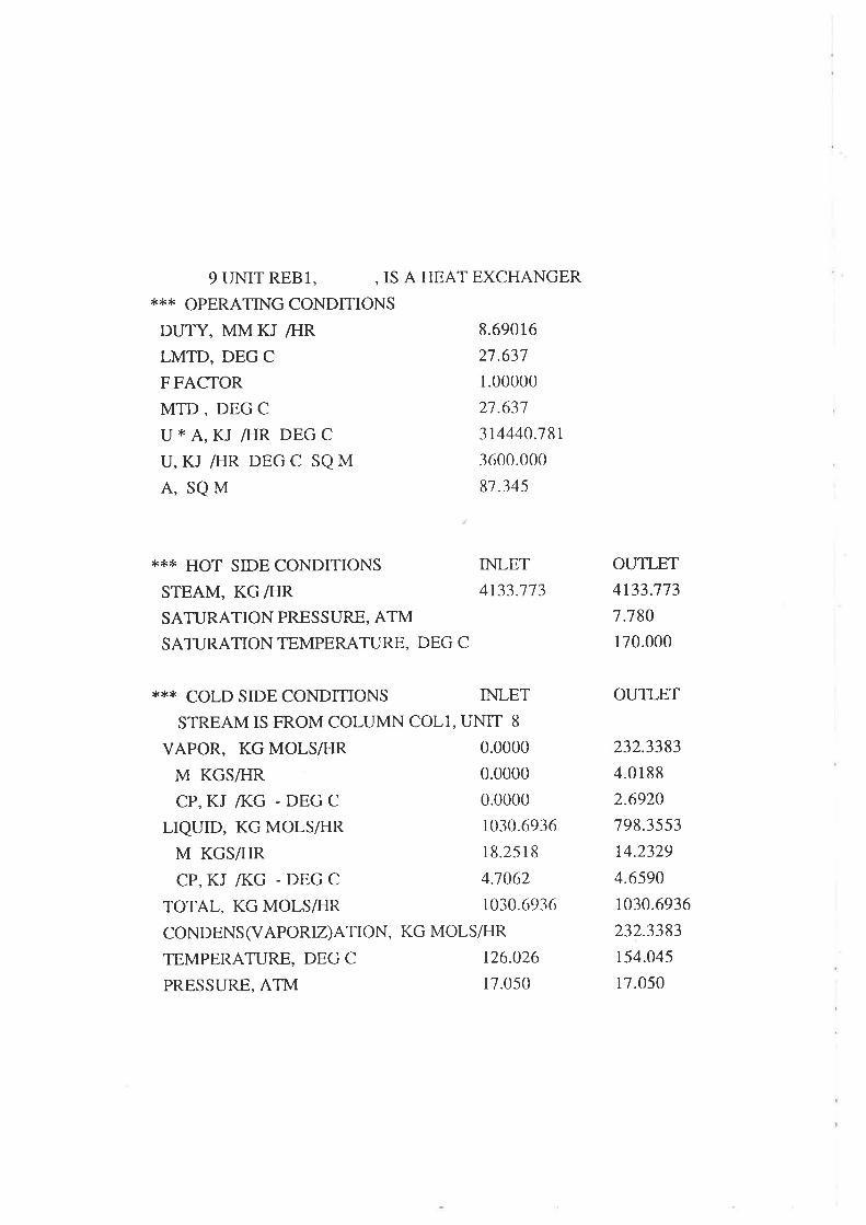
9 UNIT REBl, , IS A HEAT EXCHANGER**,K OPERATING CONDITIONS
DUTY, MM KJ ÆIR 8.69016
LMTD, DEG C 27.637
F FACTOR I.OOOOO
MTD, DEGC 21.637
U * A, zu ÆIR DEG C 314440.]81
u, KJ /HR DEG C SQ M 3600.000
A, SQ M 81.345
"{<" HOT SIDE CONDITIONS INLET
STEAM, KG ÆIR 4133.'113
SATURATION PRESSURE, ATM
SATURATION TEMPERATURE, DEG C
**" COLD SIDE CONDITIONS INLET
STREAM IS FROM COLUMN COLI, UNIT 8
VAPOR, KG MOLS/HR O.OOOO
M KGS/FIR O.OOOO
CP, KJ Æ(G - DEG C O.OOOO
LIQUID, KG MOLS/FIR 1030.6936
M KGSÆIR 18.2518
CP, KJ û(G - DEG C 4.7062
TOTAL, KG MOLSÆIR 1030.6936
CONDENS (VAPORIZ)ATION, KG MOLS/FIR
TEMPERATURE, DEG C 126.026
PRESSURE, ATM 17.050
OUTLET
4133.773
7.780
170.000
OUTLET
232.3383
4.0188
2.6920
798.3553
14.2329
4.6s90
1030.6936
232.3383
r54.045
17.050
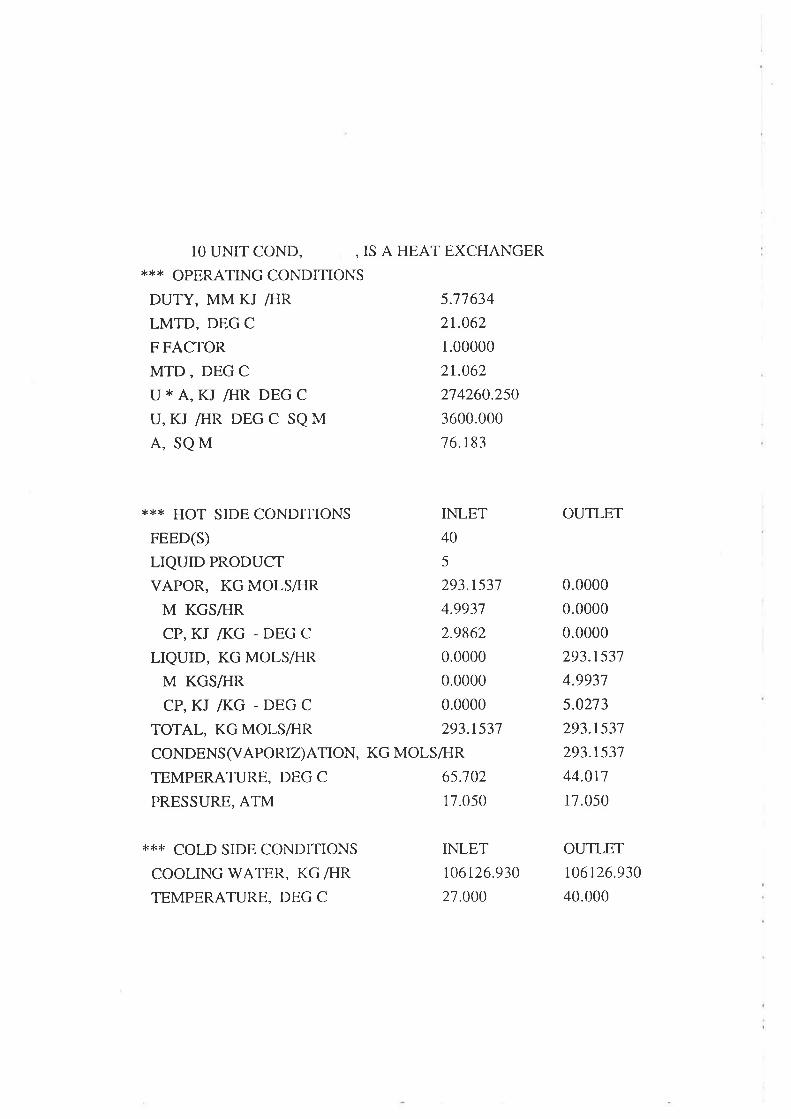
10 UNIT COND, , IS A HEAT EXCHANGER*X* OPE&{TING CONDITIONS
DUTY, MM KJ ÆIR 5.77634
LMTD, DEG C 2I.062
F FACTOR I.OOOOO
MTD, DEGC 2I.062
U * A, KJ /FIR DEG C 2]4260.250
u, KJ /HR DEG C SQ M 3600.000
A, SQ M 16.183
*** HOT SIDE CONDITIONS INLET
FEED(S) 40
LIQUID PRODUCT 5
VAPOR, KG MOLS/FIR 293.T537
M KGSÆIR 4.9937
CP, KJ Æ(G - DEG C 2.9862
LIQUID, KG MOLSÆIR 0.0000
M KGS/HR O.OOOO
CP, KJ Æ(G - DEG C O.OOOO
TOTAL, KG MOLS/HR 293.1531
CONDENS O/APORIZ)ATION, KG MOLS/FIR
TEMPERATURE, DEG C 65.]02
PRESSURE, ATM 17.050
OUTLET
0.0000
0.0000
0.0000
293.1537
4.9931
5.0273
293.1537
293.1537
44.017
17.050
*** COLD SIDE CONDITIONS
COOLING WATER, KG /I]RTEMPERATURE, DEG C
INLET
t06r26.930
21.000
OUTLET
106t26.930
40.000

S UMMARY OF COM PRES S ORÆXPANDER/PUMPÆURB INE UNITS
2 UNIT PPl , , IS A PUMP*** FEED STREAMS ARE 8
*.*X LIQUID PRODUCT IS STREAM 4
*** OPEL{TING CONDITIONS
V/ORK, KW
EFFICIENCY, PERCENT
MOLE FRACTION LIQUID
TEMPERATURE, DEG C
PRESSURE, ATM
HEAD, M
HOT VOLUME, M3ÆIR
6 UNIT P2 , , IS A PUMP,.*'< FEED STREAMS ARE 11
'<i<X LIQUID PRODUCT IS STREAM 12
*X* OPERATTNG CONDITIONS
V/ORK, KW
EFFICIENCY, PERCENT
MOLE FRACTION LIQUID
TEMPERATURE, DEG C
PRESSURE, ATM
HEAD, M
HOT VOLUME, M3/FIR
1.04
60.00
INLET
1.0000
-10.000
2.8154
1.548
15.56
INLET
1.0000
44.0tr
2.69s4
23.023
OUTLET
1.0000
-9.4t3
17.1000
315.1443
1.548
60.00
OUTLET
1.0000
44.438
17.1000
3t3.6260
23.024

UNIT ID
SEQ NO
R( 1)
R( 2)
R( 3)
R( 4)
R( 5)
R( 6)
R( 7)
R( 8)
FAST METHOD
SURE METHOD
2 COLUMN SUMMARY
TRAY TEMP PRESSURE
SUMMARY OF CALCULATOR UMTS
REPORT OF RESULTS VECTORS
CALl
I2
1.07819E+02
4.347278+02
5.080318+03
2.812618+06
4.466548-0r
3.305598+06
6.118268+06
UNDEFINED
I SUMMARY FOR COLUMN UNIT 8 - COLI,
1 TOTAL NUMBER OF ITERATIONS
0
1
2
3
4
5
6
1
DEG C
65.7
105.7
113.9
1 15.0
116.9
126.0
154.0
ATM
17.05
17.05
17.05
17.05
17.05
17.05
17.05
150
NET FLOW RATES, KG MOLS/FTR
LIQUID VAPOR FEED PRODUCT
33.4 59.5 293.2V
21.8 261.0
21.3 26r.4
1042.5 260.9 1032.0M
1039.3 244.2
1030.7 240.9
232.3 798.3L
IIEAT(COOL)ER
DUTY MM kJ/hr
8.6902
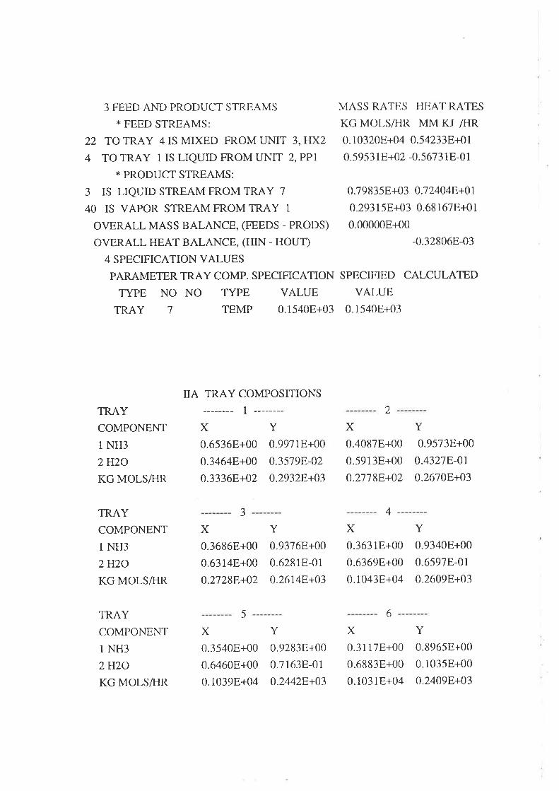
3 FEED AND PRODUCT STREAMS MASS RATES HEAT RATES
* F.EED STREAMS: KG MOLS/HR MM KJ /HR
22 TO TRAY 4IS MIXED FROM UNIT 3,HX2 0.10320E+04 0.542338+Ol
4 TO TRAY 1 IS LIQUID FROM UNIT 2,PPr 0.59531E+02 -0.567318-01
* PRODUCT STREAMS:
3 IS LIQUID STREAM FROM TRAY 1 0.798358+03 0.724048+01
40 IS VAPOR STREAMFROMTRAY 1 0.29315F+{3 0.68167E+01
OVERALL MASS BALANCE, (FEEDS - PRODS) 0.00000E+00
OVERALL HEAT BALANCE, (HIN - HOUÐ -0.32806E-03
4 SPECIFICATION VALUES
PARAMETER TRAY COMP. SPECIFICATION SPECIFIED CALCULATED
ryPE NO NO TYPE VALUE VALUE
TRAY 7 TEMP 0.1540E+03 0.1540E+03
TRAY
COMPONENT
1 NH3
zH20KG MOLS/HR
IIA TRAY COMPOSITIONS
1 -------- 2
X
0.65368+00
0.3464E+00
0.33368+{2
Y
0.9911E+00
0.35198-02
0.29328+03
X0.4087E+00
0.5913E+00
0.21788+02
Y
0.9573E+00
0.43278-0r
0.26708+03
TRAY
COMPONENT
1 NH3
2Hzo-
KG MOLS/HR
J 4
X0.36868+00
0.63148+00
0.27288+02
Y
0.9376E+00
0.62818-01
0.26148+03
X0.36318+00
0.63698+00
0.1043E+04
Y
0.9340E+00
0.6s97E-01
0.2609E+03
TRAY
COMPONENT
1 NH3
2Hzc-
KG MOLS/FIR
5 6
X
0.3540E+00
0.6460E+00
0.1039E+04
Y
0.92838+00
0.7163E-01
0.24428+03
X
0.31178+00
0.68838+00
0.10318+04
Y
0.8965E+00
0.1035E+00
0.24098+03

TRAY
COMPONENT
1 NH3
2H2o-
KG MOLSÆ]R
7
X
0.19028+00
0.8098E+00
0.7983E+03
Y
0.12928+00
0.27088+00
0.23238+03
STREAM COMPONENT FLOW RATES - KG MOLS/HR
STREAMID 3 4 5 6
PHASE LIQUID LIQUID LIQUID LIQUID
1 NH3 151.8803 58.4794 292.1052 151.8812
2H20 646.4661 1.0517 1.0485 646.4652
TOTALS 798.3464 59.5311 293.1537 798.3464
TEMPERATURE, DEG C 154.0498 -9.4127 44.0166 55.7352
PRESSURE, ATM 17.0500 17.1000 17.0500 17.0500
H, MM KJ ÆIR 7.2404 -0.0567 1.0404 1.0499
MOLE FRACT LIQUID 1.0000 1.0000 1.0000 1.0000
RECYCLE CONVERGENCE O.OOOO O.OOOO O.OOOO O.OOOO
STREAM ID
PHASE
1 NH3
2H20TOTAT-S
TEMPERATURE, DEG C
PRESSURE, ATM
H, MM KJ /FIR
MOLE FRACT LIQUID
RECYCLE CONVERGENCE
7
VAPOR
233.6217
0.0009
233.6226
-10.0000
2.8154
4.9823
0.0000
0.0000
8
LIQUID
58.4194
1.0517
59.531 1
-10.0000
2.8r54
-0.0605
1.0000
0.0000
11
LIQUID
385.5029
646.466r
1031.9690
44.0t09
2.6954
-0.8225
1.0000
0.0000
I2LIQUID
385.5029
646.466r
1031.9690
44.4375
17.1000
-0.1665
1.0000
0.0000

STREAM ID
PHASE
1 NH3
2Hzo.
TOTALS
TEMPERATURE, DEG C
PRESSURE, ATM
H, MM KJ /HR
MOLE FRACT LIQUID
RECYCLE CONVERGENCE
15
MIXED
385.5029
646.466r
1031.9690
67.7289
2.81s4
6.032
0.8267
0.0000
22
MD(ED
385.5029
646.466r
1031.9690
114.1615
17.1 000
5.4233
0.9848
0.0000
40
VAPOR
292.1052
1.0485
293.1537
65.70r7
17.0500
6.8t67
0.0000
0.0000

PROCESSru Input and Outnut File Listings
BASIC NOVEL ABSORPTION CYCLE HEATPUMP
WITH CYCLOHEXANB AND ANILINE
196

TITLE PROJECT=POWER, DATE=8-7-90
TOLER PROP=0.0005,TEMP=-0.002,STREAM=0.0005,-0. 1
DIMENS ION SI,TEMP:C,PRES S URE=MMHG
PRTNT INPUT=NONE
CALCULATON FLASH=O
COMP DATA
LIBID 1,CH/2,ANLN
TT{ERMO DATA
TYPE KTYP=LACT,HTYP=LIB RARY,S TYP=LK
KSET SETNO=I,NOTEMP=3
SUBSET 1,10.0
NRTL r ,2,,683 .9J 56,,547 .9851 ,0.4107 6
SUBSET 2,30.0
NRTL r,2,,692.3 542,,499.47 34,0.4707 6
SUBSET 3,5O.OO
NRTL r,2,,7 00.7 328,,450.9616,0.4107 6
HLSET SETNO=I,KSET=1
STREAM DATA
PROPERTY S TRM= Z,TEMP =25, PRE S = 1 500, RATE=5 3 2,COM P =1,87'0 /2,I3.0
PROPERTY S TRM= l,TEMP:2 5, PRES = 1 500, RATE=25 8 9,COM P =1,21 .0 /2,7 3.0
PROPERTY S TRM=5,TEMP= 1 00,PRE S = 1 500, RATE=31 3,COM P= 1, 8 2. 5 /2,11 .5
PROPERTY STRM=9A,TEMP= 1 O4,PRES = 1 500,RATE =27 48,COMP= 1, 3 1. 1 /2,68.9
UNTT OPERATTONS
HX UID=HXI
COLD FEED=2,L=3
HOT FEED=5,L=6
SPEC HOCI=2
FLASH UID=FI
FEED 3
PROD V:4,L=5
TPSPEC TEMP=100
S PEC STRM=5, RATE=O. 90,REFS =3
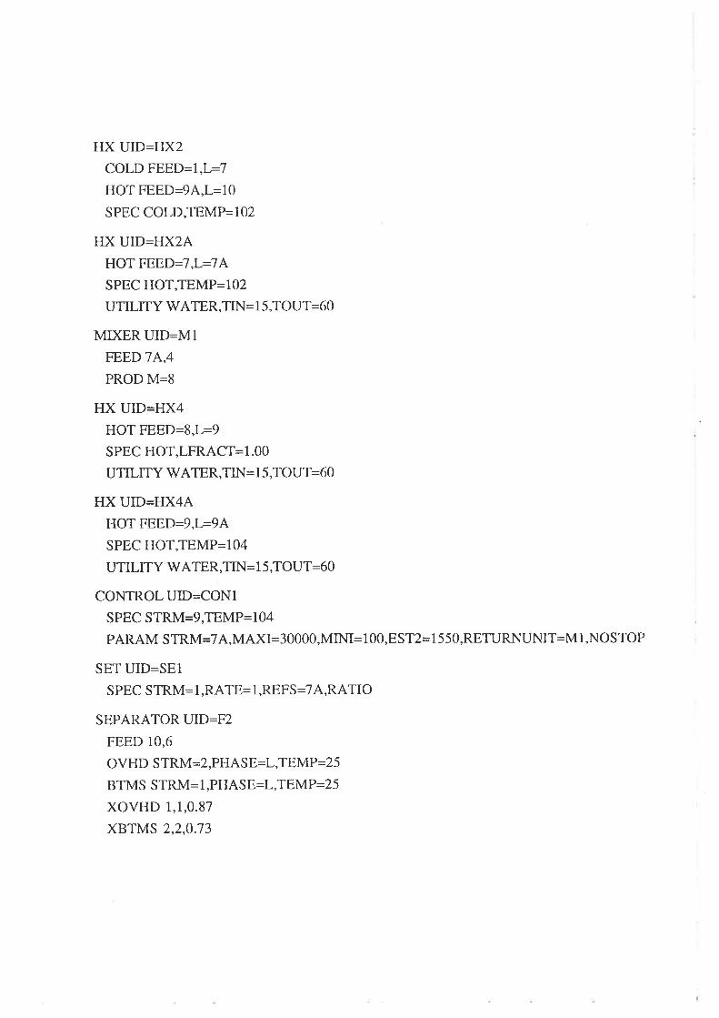
HX UID=HX2
COLD FEED=I,L=7
HOT FEED:9A,L=10
SPEC COLD,TEMP=I02
HX UID=HX2A
HOT FEED=1 ,L=7 A
SPEC HOT,TEMP=L02
UTILIY V/ATER,TIN= I 5,TOUT=60
MIXER UID=MIFEED 74,4
PROD M=8
HX UID=HX4
HOT FEED=8,L=9
SPEC HOT,LFRACT=1.00
UTILITY WATER,TIN= I 5,TOUT=60
HX UID=HX4A
HOT FEED=9,L=9A
SPEC HOT,TEMP=IO4
UTILITY WATER,TIN= 1 5,TOUT=60
CONTROL UID=CONI
SPEC STRM=9,TEMP=104
PARAM STRM=7A,MAXI=30000,MINI= 100,EST2= I 55O,RETURNUNIT=M l,NOSTOP
SET UID=SEI
SPEC STRM= 1,RATE= l,REFS=7A,RATIO
SEPARATOR UID=F2
FEED 10,6
OVHD STRM=2,PHAS E=L,TEMP=25
BTMS STRM= l,PHASE=L,TEMP:25
xovHD 1,1,0.87
XBTMS 2,2,0.J3

CALCULATOR UID=CALI
RETRIEVE P( I),UNTT=F I,DUTY
RETRIEVE P(2),U NTI=HX4,D UTY
PROCEDURE
$ R(1) rS COEFFICIENT OF PERFORMANCE
R(1)=P(2)/P(1)
RETURN
OITIIMIZER UID=OPTI
OB JECTryE UNTI=CAL 1,RES ULT,IDNO= I,MAXIMISE
PARAMETER UNIT=F 1,S PEC,MAXI=O.98,MINI=O.5,EST2=0. 85,S TEPSIZE=O.05
OPTPARA METHOD= I,IPRINT= 1
RECYCLE
LOOP NO= l,START:HX l,END=F l,TRIAL=l0LOOP NO=2,S'|ART=HX2,END=S E l,TRIAL= 10
LOOP NO=3,START=HXI,END=F2,TRIAL=10

STRM: 1 T= 25.0 P= 1228.1RATE=O.12798+05 DTEMP= 0.00 DCOMP= 0.0000
UNIT 11, CALI, SOLVED** AFIER 6 CYCLES** ALL NEW PARAMETERS SAME AS CYCLE 4 **
OPTIMIZATION HISTORY
CYCLEI2345PARA 1 9.0000E-01 8.5000E-01 8.0000E-01 7.5000E-01 7.00008-01
oBJ. 5.1449E-01 5.26808-01 5.30078-01 5.3r748-0t 5.32s28-0r
OPTIMIZATION HISTORY
CYCLE 6
PARA 1 6.5000E-01
oBJ. 5.3091E-01** BEST OBJECTIVE FUNCTION = 5.325178-01 AT CYCLE NUMBER 5
UNIT 12, OPTI, NOT SOLVED
UNIT z,FI , SOLVED
LOOP 1 NOT SOLVED AFI-ER 1 TzuALS
STRM: 5 T= 100.0 P= 1230.2 RATE= 3778. DTEMP: 0.00 DCOMP= 0.0845
UNTT 1, FIXT , SOLVED
UNIT z,FT , SOLVED
LOOP 1 SOLVED AF-TER 2 TRIALS
UNTT 3,HX2, SOLVED
UNIT 4,HX2A, SOLVED
UNIT 5, Ml , SOLVED
UNIT 6,HX4, SOLVED
UI\IIT '7,HX4A, SOLVED
CONTROLLER UNIT 8, CONI, AT ITERATION 1
SPECIFICATION VALUE : 0.104008+03, CALC = 0.104028+03
PARAMETER CURRENT = 0.110298+05, NEXT = 0.1 lO29E+05
UNIT 8, CONI, SOLVED
UNIT 9, SEl , SOLVED
LOOP 2 SOLVED AF|ER 5 TRIALS
STRM: 9A T= 104.0 P= 1228.I RATE=0.12398+05 DTEMP=0:00 DCOMP=0:0000
UNIT 10, F2 , SOLVED
LOOP 3 SOLVED AFTER 1 TRIALS
sTRM: 2 T= 25.0 P= 1228jRATE= 4540. DTEMP= 0.00 DCOMP= 0.0002
STRM: 1 T= 25.0P= 1228.1RATE=0.1103E+05 DTEMP=0.00 DCOMP=0.0000
UNIT 11, CAL1, SOLVED
UNIT 12, OP'fl, SOLVED

***,* PROBLEM SOLUTION REACHED *t<**
VERSION 0484 SM
SIMULATION SCIENCES, INC. PROCESS
PROJECT POWER
PROBLEM SOLUTION 8.7-90
PAGE 4
SUMMARY OF FLASH DRUMS,MIXER/SPLITTERS AND VALVES
UNIT ID
SEQ NO
TYPE
FEEDS
PRODUCTS
TEMP, DEG C
PRESSURE, MMHG
FRACTION LIQUID
DUTY, MM zu /HR
F1
2
FLASH
3
4 Cv)
5 (L)
100.0000
t230.166t
0.70000
57.47249
M1
5
MIXER
7A
4
8 (M)
106.1630
1228.0967
0.92246
0.00000

SUMMARY OF HEAT EXCHANGE UNITS
1 UNIT HXl , , IS A HEAT EXCHANGER*,<* OPERATING CONDMONS
DUTY, MM KJ /FIR 39.56242
LMTD, DEG C 8.398
F FACTOR I.OOOOO
MTD, DEGC 8.398
U * A, KJ /HR DEG C 4710785.000
**:K HOT SIDE CONDITIONS INLETFEED(S) 5
LIQUID PRODUCT
VAPOR, KG MOLSÆIR O.OOOO
M KGSÆIR O.OOOO
CP, KJ /KG - DEG C O.OOOO
LIQUTD, KG MOLS/FIR 3117.8614
M KGSÆIR 272.4743
CP,zu /I(G -DEGC 2.1444TOTAL, KG MOLSÆ{R 317].86]4CONDENS(VAPORIZ)ATION, KG MOLSÆIR
TEMPERATURE, DEG C IOO.OOO
PRESSURE, MMHG 1230.174
OUTLET
6
0.0000
0.0000
0.0000
3117.8674
272.4743
t.1779
3177.8674
0.0000
27.000
t230.r74
OUTLET
3
0.0000
0.0000
0.0000
4539.0259
387.34s8
2.0374
4539.0259
0.0000
71.717
1228.091
'ß*,, COLD SIDE CONDITIONS INLETFEED(S) 2
LIQUID PRODUCT
VAPOR, KG MOLS/FIR O.OOOO
M KGSÆIR O.OOOO
CP, KJ /KG - DEG C O.OOOO
LIQUTD, KG MOLSÆIR 4539.0259
M KGSÆIR 387.3458
CP, KJ Æ(G - DEG C 1.8009
TOTAL, KG MOLSÆ{R 4539.0259
CONDENS(VAPORZ)AÏON, KG MOLS/FrR
TEMPERATURE, DEG C 25.OOO
PRESSURE, MMHG 1228.097

3 UNIT HX2 , , IS A HEAT EXCHANGER*** OPERATING CONDTTIONS
DUTY, MM KJ ÆIR 137.94337LMTD, DEG C 5.915F FACTOR I.OOOOO
MTD, DEGC 5.915
U * A, KJ ÆIR DEG C 23319504.000
{<X:K HOT SIDE CONDINONS INLETFEED(S) 9A
LIQUID PRODUCT
VAPOR, KG MOLS/FIR O.OOOO
M KGSÆIR O.OOOO
CP, KJ /I(G - DEG C O.OOOO
LrQUrD, KG MOLS/FrR 12390.7490M KcSÆrR 1115.8488
CP, KJ Æ(G - DEG C 2.1479TOTAL, KG MOLS/FIR 12390.]490CONDENS0/APORIZ)ATION, KG MOLS/FIRTEMPERATURE, DEG C 1O4.OOO
PRESSURE, MMHG 1228.097
OUTLET
10
0.0000
0.0000
0.0000
12390.7490
1115.8488
1.5 882
t2390.7490
0.0000
38.r32
1228.097
*** COLD SIDE CONDITONS INLETFEED(S) 1
LTQUID PRODUCT
VAPOR, KG MOLS/HR O.OOOO
M KGSÆìR O.OOOO
CP, KJ /I(G - DEG C O.OOOO
LIQUID, KG MOLSÆIR 1t029.0400M KGSÆ{R 1000.9313
CP, KJ Æ(G - DEG C 1.5932
TOTAL, KG MOLS/FIR IIO29.O4OO
CONDENS (VAPORTZ)ATrON, KG MOLS/FrRTEMPERATURE, DEG C 25.OOO
PRESSURE, MMHG T228.097
OUTLET
7
0.0000
0.0000
0.0000
11029.0400
1000.9313
2.1 185
r 1029.0400
0.0000
102.000
t228.097

4 UNIT HX2A, , IS A HEAT EXCHANGER
tX*T. OPERATING CONDITIONS
DUTY, MM KJ ÆIR
LMTD, DEG C
F FASTOR
MTD, DEG C
U*A,KJÆIR DEGC
0.00000
67.793
1.00000
6r.793
0.000
*** HOT SIDE CONDITTONS INLETFEED(S) 7
LIQUID PRODUCT
VAPOR, KG MOLS/HR O.OOOO
M KGS/HR O.OOOO
CP, KJ Æ(G - DEG C O.OOOO
LIQUTD, KG MOLSÆIR 11029.0400
M KGS/FIR 1000.9313
CP, KJ A(G - DEG C 2.1185
TOTAL, KG MOLS/I-IR ITO29.O4OO
CONDENS(VAPORIZ)ATION, KG MOLSÆIR
TEMPERATURE, DEG C 1O2.OOO
PRESSURE, MMHG 1228.097
OUTLET
7A
0.0000
0.0000
0.0000
rr029.0400
1000.9313
2.1185
11029.0400
0.0000
102.000
1228.091
)l
I
).r
).r
).r
T2
tlz.
I2
)(1C
t2*** COLD SIDE CONDITIONS
COOLING WATER, KG /HRTEMPERATURE, DEG C
INLET
0.000
15.000
OUTLET
0.000
60.000oì
1(
6C


7 UNIT HX4A, , IS A HEAT EXCHANGER
*'ß* OPERATING CONDMONSDUTY, MM KJ /HRLMTD, DEG C
F FACTOR
MTD, DEG C
U*A,KJ /FIR DEGC
0.12034
63.891
1.00000
63.89 1
1883.569
*,** HOT SIDE CONDMONS INLETFEED(S) e
LIQUID PRODUCT
VAPOR, KG MOLSÆIR O.OOOO
M KGS/FIR O.OOOO
CP, KJ Æ(G - DEG C O.OOOO
LrQUrD, KG MOLS/FIR 12390.7471
M KGSÆIR 1115.8486
CP, KJ /I(G - DEG C 2.T155
TOTAL, KG MOLSÆIR 12390.7 47
CONDENS (VAPORIZ)AION, KG MOLSÆrR
TEMPERATURE, DEG C 104.018
PRESSURE, MMHG 1228.097
OUTLET
9A
0.0000
0.0000
0.0000
12390.747r
1115.8486
2.r479
12390.7471
0.0000
104.000
1228.097
*** COLD SIDE CONDITIONS
COOLING WATER, KG Æ{R
TEMPERATURE, DEG C
TNLET
638.144
15.000
OUTLET
638.144
60.000

SUMMARY OF COMPONENT SEPARATORS
F2
10
UNIT ID
SEQ NO
NAME
FEEDS
PRODUCTS
TEMP, DEG C
PRESSURE, MMHGFRACTION LIQUIDDUTY, MM KJ /HR
2 (L) 1 (L)
25.0000 25.0000
1228.A967 1228.0967
1.00000 1.00000
27.00710
SUMMARY OF CALCULATOR UNITSREPORT OF RESULTS VECTORS
CALl11
5.28008E-01
UNDEFINED
UNDEFINED
UNDEFINED
UNDEFINED
UNDEFINED
UNDEFINED
UNDEFINED
10
6
UNIT ID
SEQ NO
NAME
R( 1)
R( 2)
R( 3)
R( 4)
R( 5)
R( 6)
R( 7)
R( 8)
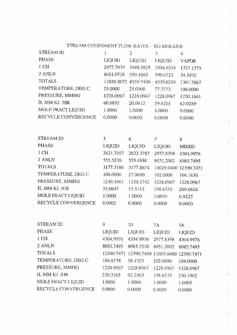
STREAM COMPONENT FLOW RATES -
STREAM ID I 2
PHASE LIQUID LIQUID1 CH 2977.7939 3949.58252 ANLN 8051.0728 590.1665
TOTALS 11028.8612 4539.1490TEMPERATURE, DEG C 25.OOOO 25.OOOO
PRESSURE, MMHG 1228.0967 1228.0967
H, MM zu ÆlR 60.6893 20.0612
MOLE FRACT LTQUID 1.0000 1.0000
RECYCLE CO}IVERGENCE O.OOOO O.OOO2
KG MOLS/FIR
34LTQUID VAPOR
3948.9534 t327.t57s590.0723 34.5492
4539.0259 t361.7067
17.7772 100.0000
1228.0967 1230.166r
59.6211 62.0289
1.0000 0.0000
0.0000 0.0000
STREAM ID
PHASE
1CH
2 ANLN
TOTALS
TEMPERATTIRE, DEG C
PRESSURE, MMHGH, MM KJ ÆIR
MOLE FRACT LIQUID
RECYCLE COIN/ERGENCE
STREAM ID
PHASE
1CH
2 ANLN
TOTALS
TEMPERATURE, DEG C
PRESSURE, MMHG
H, MM KJ /FIR
MOLE FRACT LIQUID
RECYCLE CONVERGENCE
5
LIQUID
762t.7957
555.5230
3177.3186
i00.0000
1230.166r
55.0647
1.0000
0.0002
6
LIQUID
2622.3781
555.4886
3777 .867 4
27.0000
1230.r742
15.5113
1.0000
0.0000
7
LIQUID
2977.8398
80s 1.2002
11029.0400
102.0000
1228.0967
198.6335
1.0000
0.0000
8
MD(ED
4304.9976
8085.7495
12390.7471
106.1630
1228.0967
260.6624
0.9225
0.0000
9
LIQUID
4304.9976
8085.7495
12390.7471
104.0178
1228.0967
230.3165
1.0000
0.0000
10
LIQUID
4304.9916
8085.75 r0
12390.7490
38.1323
1228.0967
92.2463
1.0000
0.0000
7A
LIQUTD
2917.8398
8051.2002
11029.0400
102.0000
1228.0967
198.6335
1.0000
0.0000
9A
LIQUID
4304.9976
8085.7495
12390.7471
104.0000
1228.0967
230.t962
1.0000
0.0000

BIBLIOGRAPHY
Abello, L., servais, 8., Kern, M. and pannetier, G., "stuclies of Hydrogen Bonding N_
H..N. X[[- Thermodynamic Study of the Self Association of Aniline c¿ncl N-Methylaniline
inCyclohexane", BuIl. Soc. Chim. Fr., ll, 4360 (1968)
Altenkirch, 8., Absorptionskaltemaschinen, vEB - verlag Technik, Berlin (1954)
Ando, E. and Takeshita, L, "Residential Gas-Fired Absorption Heat Pu.ntp Based on R22-
DEGDME Pair. Part I Thermodynamic Properties of the R22-DEGDME pair", Inr. J.
Refrig., 7, 181 (1984)
Asselineau, L. and Renon, H., "Extension de l'Equation NRTL pour Ia Representation de
l'Ensemble des Donnees d'Equilibre Binaire, Liquicle-Vapeur et Liquicle-lLqu.ide", Chem.
Eng. Sci., 25, I2I1 (L970)
Auh, P.C., "A Survey of Absorption Cooling Technology in Cooling Applications", B.N.L.
Report No. 50704 (1977)
Backstrom,M., Kaltetechník, Verlag G Braun, Karlsruhe (1953)
Bett, K.8., Rowlinson, J.S. and Saville, G., Thermodynamics for Chemical Engine¿rs, MIT
Press (1975)
Blass, 8., "Capacity Increase of NH j H20 Absorption Refrigeration Plants for Industrial
Refrigeration", DKY - Tagungsbericht, Numberg, 145 (19j4)
Bogart, M., Antmonia Absorption Refrigerat¡on in Ind.u.striol Processes, Gulf pub. Co.,
(1e8 1)
Briggs, s.w., "second-Law Analysis of Abgorptíon Refrigeretion", proc. AGA & IGT
Conf. on Natural Gas Res. & Tech., Chicago (1971)
Buchner, E.H. ancl Kleyn, D., Recl. Trav. Chim. pays-Bas., 43, I53 (1924)
Buffington, R.M., "Qualitotive Requirements for Absorbent-Refi'Ìgerant Combinations",
Refrig. Eng., 57, 343 (1949)

cockshoot, J.E., Proc. 4th Aust. chem. Eng. conf., Adelaide, 330 (rg76)
Copp, J.L., "Thermodynamics of Binary Systems Containing Antínes; part 2',, Trans.
Faraday Soc., 51, 1056 (1955)
Copp, J.L. and Everett, D.H., "Thermodynamics of Binary Systems Containing Amines,. part
3", Trans. Faraday Soc., 53, 9 (1951)
Copp, J.L. and Everett, D.H., "Thermodynamics of Binary Systems Containing Am.ines,,,
Faraday Soc. Discussions, 15, 174 (1953)
Chueh, c.F. and swanson, 4.c., "Estimatíng Liquid Heat capacity", chem. Eng. progr.,
69, 83 (1973)
chun, K.w., clikscales, T.c. and Davison, R.R., "vapour-Liquid Equilibrium of
Triethylantine-Water and Methyldiethylamine-Water", J. Chem. Eng. Data, 16,443 (Igll)Dalichaouch, M., "Energy Analysis of Absorption-Refrigeration Cycles", J. Inst. Energy,
63, t6l (1990)
Davison, R.R., "Vapour-Liquid Equilibria of Water-Diisopropylantine and Water-Di-n-
Propylamine", J. Chem. Eng. Data, 13, 349 (1968)
Davison, R.R., Smith W.H. and Chun K.W., "A Static Vapour Pressure Apparatus forMixtures", AIChE Journal, 13,590 (1967)
Davison, R.R., Smith W.H: and Hood D.W., "Phase Equitibria of Desalination Solvents;
Water-NaCl-Antines", J. Chem. Eng. Data, I,304 (1966)
Davison, R.R., Smith W.H. and Hood D.W., "structure anrJ Amine-Water Sotu.bitity itt
Desalinotion by Solvent Extractiofl", J. Chem. Eng. Dara, 5,420 (1960)
Felsing, W.A. and Phillips, 8.A., "Partial Vapour Pressures of Aqueous Methylantine
Solution", J. Am. Chem. Soc., 58, 1973 (1936)
Gmehling, J., Onke¡r, U. and Arlt, W., Vapour - Liquicl Data Collection, Dechema Chemistry
Dat¿ Series, Frankfurt (1977 -)
Grover, G.S., Devotta, S. and Holland, F.4., "Performance of on Experimental Absorption
Cooler Usittg Aqueous LiCl and LiCllLiBr Solutions", lnd. Eng. Cliern. Res., 28, 250
(1 e8e)

Holldorff, G., "Revisions up Absorption Refrigerotion Efficiency", Hydrocarborr
Processing, 58, 149 (1919)
Hood, D.W. and Davison, R.R., "The Place of Solvent Extraction in Saline Water
Conversion", Aclvan. Chem. Series No 27, 40 (1960)
Hosseini, S.M. and Schneider, G., " Evaporation Equilibria in Hyclrocarbon - Aniline Systents
(III)", Z.Phys. Chem. (Frankfurt), 36, 137 (1963)
Hunter, T.G.and Brown, T., "Distribution in Hyclrocarbon-solvent Systems", Ind. Eng.
Chem., 39, 1343 (1941)
Iedema, P.D., "Mixtures for the Absorptíon Heat pump", Int. J. Refrig., 5, 262 (19g2)
Jacob, X., Albright, c.F. and rucker, w.H., "Factors Affecting the coefficient of
Petformattce for Absorption Air-Conditioning Systems", ASHRAE Trans., 75, 103
(re6e)
Joback, K.G., Thesis, Massachusetts Institute of Technology, Cambridge, Mass. (1984),
Kandlikar, S.G., "A New Absorber Heat Recovery Cycte to Improve COP of Aqua-Anulonia
Absorption Refi igeration System", ASHRAE Trans., 88, 141 (1982)
Karakas, 4., Egrican, N. and Uygur, 5., "second-Law Analysis of Solar Absorption-Cooling
Cycles using Lithium Bromidel Water and Ammonial Water as Working Fluicls", Appliecl
Energy, 37, 169 (1990)
Kauslrik, S.C. ancl Kaudinya, J.V., "Open-Cycle Solar Absorption Cooling. A Review,,,
Energy Convers. Mgmt., 29, 84 (1989)
Korteum, G. and Frier, H.J., "IsothermalVapour-Pressure Diagrams of Binary anclTernory
Liu.qu.i.d. Mixtures by a Simplified Statíc Method", Chem. Ing. Tech., 26, 670 (1954)
Kriebel, M. and Loffler, HJ., "Thermodynamische Eigenschaften des Binaren Systems R22 -
Tetra at hy le ng ly ko I d imethy lat her", Kaltetechnik, lj, 266 ( 1 965)
Kumar, R. and Kaushik, S.C., "Thermoynamic Evaluation of a moclified. Aquo-Ammonia
Absorptiort Refrigeration System", Energy Convers. Mgmt., 32, lg1 (1991)

Lange, N.4., Handbook of Chemistry l}th ed., McGraw - Hill, New York, .(1961)
Lenz, T., Loef, G., Kaushik, v. and Sandell, G., "open-Cycle solar Absorption cooling",
Proc. 9th Cong. Int. Solar Energy Soc., Montreal (1985)
Linnhoff, B. ancl Ahmad, s., "Cost optimum Heat Exchanger Networks -1. Minimum
Energy atd Capital Using Simple Models for Capital Cost", Computers Chem. Engng.,
t4, 129 (1990)
Linnhoff, B. and Carpenter, KJ., "Energy Conservation by Exergy Analysis - The Quick oncl
Simple Way", Proc. 2nd. World Cong. Chem. Eng., Montreal (1981)
Ludwig, E.E., Applied Process Design for Chemical and Petrochemical Plants, Gulf Pub.
Co. (1965)
Macriss, R.4., "S¿lect¡ng Refrigerant Absorbent Fluid Systems for Solar Energy Utilization",
ASHRAE Trans., 82, 975 (1976)
Maiuri, G.,2. f. ges Kalte Ind., 46, 169 (1939)
Manscori, G.A. and Patil, V., "Thermodynamíc Basisfor the Choice of Workíng Fluidsfor
Solar Absorptiott Cooling Systems", Sola¡ Energy, 22, 483 (1979)
Mehta, G.D., "Liquid. Phase Separation in Absorption RefrÌgerotion", U.S. Patent No.
4,283,918 (1981)
Morrissey, A.J. and O'Donnell, J.P., "Endothermic Solutions and their Applicatiott in
Absorption Heat PLtmps", Chem. Eng. Res. Des., 64, 404 (1986)
O'Neill, B.K. and Roach, J.R., "Organic-Fluid Absorption-Cooling Systems; An Assessntent
of the Theoretical Performance Limits", Proc. 18th Aust. Chem. Eng. Conf., Aucklancì,
330 (1ee0)
Peters, M.S. and Timrnerhaus, K.D., Plant Design and Economics for Chentical
Engineers, McGraw-Hill (1991)
Press, w.H., Flanrrery, 8.P., Teukolsky, S.A. and vetterling, w.T., Numerical Recipes;
The Art of Scientific Computing, Cambridge University Press (1989)

Reid, R.C., Prausr.ritz, J.M. and Poling, 8.8., The Properties of Goses & Liquids 4ecl,
McGraw Hill (1987)
Renon, H. ancl Prausnitz, J.M., "Local Compositions in Thermodynamic Excess Function's
for Liquid Mixtures", AIChE Journal, 14, I35 (1968)
Riedel, L., "Extension of the Theorem of Correspondíng States. III Critical Cofficient,
Density of SaturatedVapour, and Latent Heat of Vaporization", Chem. Ing. Tech., 26,
619 (1954)
Roeck, H. and Sieg, L., "Measurement of Evaporation Equilibria in a Modernized By-pass
Apparatus" , Z.Phys. Chem. (Frankfurt), 3, 355 (1955)
Skjold-JorgenSen, S., Rasmussen, P. and Fredenslund, AA, "On the Temperature
Depenrlence of the UniquaclUnifac Models", Chem. Eng. Sci., 35, 2389 (1980)
Stephan, K., "History of Absorption Heat Pumps and Working Pair Developments in
Europe", Int. J. Refrig., 6, 160 (1983)
Tan, T.C. ancl Ti, H,C., "Preflicting Effect of Dissolved Solute on the Vttpour-Liquid
Equilibria of Organic Solvent Mixtures and Aqueous Organic Acid Solutions", Chem. Eng.
Res. Des., 61, 79 (1989)
Ting, 4.M., Lynn, S. and Prausnitz, J.M., "Líquid-Liquid Equ.ilibria for Aqueous Systems
Containing N,N-Diethylmethylamine and Sodium Chloride or Sodiunt Sulfate", J. Chem.
Eng. Data, 37, 252 (1992)
Trepp, Ch., "Histot'y a.nd Perspectives of Heat Transþrmation", Int. J. Refrig., 6, 309
(1983)
Uemura, T. and Hasaba, S., "studies on the R22-Absorbent Absorptiotl Refrigerating
Machine", Reito, 43, l24l (1968)
Zellhoefer, G.F., "So/¿ hitity of Halogenated Hydrocarbon Refrigerants in Orgarúc Solvents" ,
Ind. Errg. Chem., 29, 548 (1931)
Ziegler, B. ancl Trepp, Ch., "Equation of State for Ammonia-Water Mixtures", Int. J'
Refrig., 7, 101 (1984)

PUBLICATIONS RESULTING FROM THTS STUDY
'White, S.D. and O'Neill, 8.K., "Phase Equilibría for Dímethylethylamine-Water and
Trimethylamine-Water Mixtures" , J. Chem. Eng. Data, in press
White, S.D. and O'Neill,8.K., "Performance of a Novel Absorption Refrígeration Cycle",
Proc. 18th Aust. Chem.Eng.Conf., Canberra, Part2,360 (1992)
White, S.D. and O'Neill, B.K., "A Novel Absorption Cycle Heat Pump; Part I -
Refrigeration", submitted to Int. J. Refrig
White, S.D. and O'Neill, 8.K., "A Novel Absorption Cycle Heat Pump; Part II - Heating",
submitted to Int. J. Refrig
White, S.D. and O'Neill, 8.K., "An Improved Absorption Refrigeration Cycle", Provisional
Patent

ADDENDA
Section 2.1. page 4. insert following paragraph before paragraph I
Plattens and Munûer modifìed the conventional absorption refrigeration cycle to eliminate the
necessity for mechanical pumping. The Electrolux domestic absorption refrigerators, which
employ this cycle, have been extremely popular in situations where electricity is not available
or is unreliable.
Section 2.3. page 8. insert following paragrapb before paragraph 1
The conventional absorption refrigeration cycle is illustrated in figure 2.1. High pressure
liquid refrigerant exiting the top of the distillation column is depressured across an expansion
valve and fed to the evaporator. The reduction in pressure causes the refrigerant to boil at low
temperature. Consequently, useful refrigeration is obtained by boiling the refrigerant in the
evaporator. The resulting low pressure refrigerant vapour is dissolved/condensed in lean
absorbent at low pressure. Refrigerant rich absorbent, exiting the absorber, is then pumped
back to high pressure and the refrigerant is recovered from the absorbent in the distillation
column. Improved efficiency can be obøined by (i) preheating the distillation column feed
with hot lean absorbent exiting the bottom of the distillation column and (ii) precooling liquid
refrigerant with cold refrigerant vapour exiting the evaporator (figure 8.1).
Section 3.1.2. page 28. insert following paragraph before paragraph 2
Within the accuracy of the experimenøl technique, there was no change in the measured
concentrations when the mixture was allowed a longer equilibration time.

Section 6.3. page 91. Insert new section 6.3.4 as follows
6.3.4 Exergy Analysis of the Varlations to the Novel Absorption Cycle.
The performance of a number of variations of the novel absorption refrigeration cycle have
been examined using dimethylethylamine and water as the refrigerant and absorbent
respectively. Unfortunately, the performance of each novel cycle variation was shown to be
inferior to the conventional absorption refrigeration cycle. In an attempt to explain the
decline in performance obtained with the novel cycle variations, an exergy analysis has been
performed on each of the cycles examined.
To enable exergy losses in each cycle to be compared, the evaporaûor temperature and duty
were set at l5oC and 0.7 MW. Process data, for each variation analysed, are presented in
figures 6.5,6.6,6.8 and 6.10. St€am at ll0oC was used as the heat source and heat was
rejected ûo an ambient temperature of 20"C. The simplified equations presented by Linnhoff
and Carpenter (19f11) were used for calculating exergy losses in each unit. Exergy losses for
each cycle variation are presented in table 6.1.
Comparison of the total exergy losses incurred in each cycle can be used to rank the
thermodynamic perforlnanæ of the cycles. Examination of øble 6.1 confirms that exergy
losses from the conventional cycle are less than those obtained in the novel cycle variations.
The novel cycle with refrigerant rectifîcation appears to be the best of the novel cycle
variations. These results agree with the COP comparisons presented in section 6.3.3.
Examination of the source of exergy losses, in each of the cycle variations, confirms that the
addition of the liquid phase separation step has successfully led to a reduction in exergy
losses in the distillation column. Unfortunately, the resulting increase in the required
absorption fluid circulation rate has led to a significant increase in losses in the absorbent heat
recovery exchanger. Heating the absorption fluid to effect liquid phase separation also results
in significant losses.

Unit Conventional Cycle
Exergy t oss (kW)
Novel Cycle with Absorbent
Phase Distillation Exergy
Novel Cycle with Refrigerant
Phase Rectifi cation Exergy
Novel Cycle with
Evaporator Blowdown
Loss l,oss Loss
Distillation column
Absorber
Absorbent heat
recovery exchanger
Evaporaûor
Liquidliquidseparation
Liquid-liquid
sepaxatlon
ToTAL
r70.3
239.r
38.9
14.4
Æ2.7
86.0
290.2
60.2
15.1
102.8
139.7
2U.5
77.r
14.5
48.r
176.3
34r.7
88.1
629.6
23.5
neg
neg3.5
557.8 ß3.9
TABLE6.1. COMPARISON OF ÞßRGY LOSSF,S FOR NOVELCYCLE YARIATIONS

The exergy losses from the absorber is also of interest. The exergy losses in the absorber of
the refrigerant phase rectification cycle are significantly lower than those obtained in the
conventional cycle. This can be explained by the higher pressure observed in the absorber
and highlights the importance of absorber pressure on the overall performance of absorption
refrigeration cycles. This will be discussed in more detail in chapter 8.
Numerous alternative mixtures, exhibiting upper critical solution temperature phase
behaviour, could have been chosen to demonstrate the feasibility of the novel heat pump
cycles. The furfural/water absorbent/refrigerant pair is one candidate pair that may have
proved more attractive. Phase equilibrium data for this pair is presented in Appendix E.
There is a large difference between the boiling point of furfural and water and the liquid-
liquid phase envelope straddles the vapour-liquid azeotrope. This enables relatively impure
volatile working fluid to be completely boiled off in the evaporator without lowering the
boiling point difference between the evaporator and the absorber.
The boiling point difference between coexisting liquid phases must be zero. With increasing
temperature the boiling point difference will increase to enable a boiling point difference to
be obtained between the evaporator and the absorber in the novel heat pump cycle.
Unfortunately, for all conceivable mixtures, the boiling point difference does not increase
rapidly with increasing temperature. Consequently, the liquid phase separation step will
never contribute significantly to the boiling point elevation which can be achieved between
the evaporator and the absorber in these cycles.
For mixfures exhibiting upper critical solution temperature behaviour, the forces of
interaction are physical in nature. Consequently, the impact of changing temperature on
mixture properties will be small compared with the changes observed in tertiary amine-water
mixtures, which are strongly influenced by hydrogen bonding.

Add a new APpendix E as follows
APPendix E
THBRMODYNAMIC EQUILIBRIUM DATA FOR CYCLOHEXANE -
AI\IILINB AND FURF'T]RAL. WATER MIXTURES
Cyclohexane - aniline and furfur¿l - water mixtures were selecæd for further investigation as
candidate working fluid pairs in the novel heat pump cycle and its variations. While no
experimental phase equilibrium data was obtained for these mixtures, a summary of available
experimental data from the literature is presented below '
(i) Cyclohexane - Aniline
P( ) x(mole fraction) y (mole fraction)
n3.o262.2
255.5
251.2
2ß.82ß.2245.7
245.O
?A3.5
24r.3
?37.4
229.6
2r9.1
200.0
163.3
t19.2
3.47
0
0.061
o.126
o.206
o2s7o.392
0.418
0.438
0.514
0.606
o.ffio.716
o.774
0.832
0.891
o.E36
1.0
0
0.0ü/
0.0095
O.ot I0.011
0.011
0.011
0.011
0.0115
0.012
0.012
0.012
0.013
0.016
0.021
0.028
1.0
TABLEE. I : VApoUR-LIetlD EQUILIBRTUM Fl)R MTXTLIRES oF ANILINE AND CYCLOHEXANE AT
50.2"C' ABELITOET. AL (1968)

P (mmHe) x (mole fraction) y (mole fraction)
151.6
t45.2
t42.9
t4t.4I40..4
rÆ.4
139.8
139.7
r39.4
139.0
138.3
136.2
131.3
116.1
105.8
1.3
0
0.063
0.111
0.16ó
o.267
0.304
o.3yo.4v0.530
0.606
0.638
0.708
o.773
0.853
0.883
1.0
0
0.005
0.0û7
0.008
0.008
0.008
0.008
0.008
0.008
0.008
0.008
0.0085
0.009
0.010
0.012
1.0
TABLEE 2 : YAPOUR-LIQLID EQTIILIBRIUM FoR MIXTURES oF ANILINE AND CYCLOHEXANE AT
35.2"C, ABELLOET. AL (1968)
P (mmHe) x (mole fraction) y (mole fraction)
511.06
ffi.v2Æ9.41
478.79
46,9.M
Ær.33
452.18
439.K
413.30
385.35
343.62
315.79
0.0910
0.1130
0.2110
o.3235
o.4278
0.5100
o.5720
o.63t4o.7353
o.7879
0.8385
0.8630
0.0116
o.or27
0.0154
0.0169
0.0180
0.0186
o.oly20.0200
o.0216
o.0236
o.0270
o.0299
TABLEB 3 : VAPOUR.LIQI.ID EQUILIBRITJM FOR MIXTURES OF ANILINE AND CYCI,OHEXANE AT
7o.0oc, HOSSETNI AND SCHNEIDER (196:t)
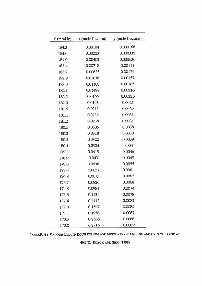
P (mmHe) x (mole fraction) y (mole fraction)
r8r'..3
l&1.0
r&+.0
183.4
r83.2
t82.9
183.0
t82.3
182.2
182.0
181.5
181.1
t8r.2180.5
180.2
180.4
180.1
179.2
178.9
178.0
177.O
fl6.4t75.7
174.8
r73.6
r72.4
172.O
17t.lt70.3
170.0
0.00104
0.00203
0.00402
0.00718
0.00825
0.01036
0.01108
o.ot499
0.0156
0.0143
o.o2t3
o.0232
0.0238
0.û305
0.0318
o.u322
o.0324
0.0419
0.043
0.0536
o.0r,57
0.0675
0.0826
0.0981
0.1134
o.r4t2o.t5w0.1958
o.2365
o.nß
0.000168
0.000332
0.000ó36
0.00111
0.00124
0.00157
0.00165
0.00216
o.æ225
0.0021
0.0029
0.0031
0.0031
0.0038
0.0039
0.0039
0.004
0.004ó
0.0049
0.0055
0.0061
0.0062
0.0068
0.0074
0.0078
0.0082
0.00&t
0.0087
0.0088
0.0089
TABLEE 4 : VAPOUR-LIQLID EQUILIBRIUM FoR MiXTURF,S oF ANILINE AND CYCLOHEXANE AT
40.0oc, RoEcK AND SIEG (195Ð

(ii) Furfural - Water
T('c) x(mole fraction) y (mole fraction)
r6t.7158.8
154.8
IÆ.O
r22.5
109.5
100.6
98.7
97.9
98.07
98.56
r00
0
o.o2
0.04
0.06
0.08
0.1
o.2
0.3
0.96
0.!ao.99
1.0
0
0.1
0.19
0.36
0.68
0.81
0.89
0.905
0.908
o.92
0.945
1.0
TABLEE. 5 : VAPOUR-LIQUID EQUILIBRIUM FoR ll[IxTURES oF FURFLJRAL AND WATER AT
760MMHG, MArNS(r922)
T("C) x(mole fraction) y (mole fraction)
85.4
42.2
Æ.6
Æ.2
4.4n.74.94r.2
0
0.0981
o.2tE2
o.q796
0.9911
o.9962
0.9981
1.0
0
0.9154
o.9202
o.v275
o.9426
o.9674
0.9805
1.0
TABLEE. 6 : VAPOUR.LIQUID EQIIILIBRIUM FOR MIXTURES OF FI.JRFURAL AND WATER AT
ssMMHG, TSIRLIN (1962)

T ("C) x (mole fraction) y (mole fraction)
r53.2
t23.O
100.0
92.7
91.8
91.5
91.7
v2..2
E2.8
93.2
93.3
0
0.0981
o.2tv2
o.3721
0.4&18
o.9679
o.9796
0.9911
o.9962
0.99f31
1.0
0
0.s557
0.831l
0.9008
0.9079
0.9115
o.9206
o.9443
o.v732
0.9875
1.0
TÀBLEE. 7 : YAPOUR-LIQTID EQTIILIBRII.,M FOR MIXTURES OF FURFTJRAL AND WATER AT
ó00MMHG, TsrRLrN (1962)
ERRATA
Section 2.3. page 8. paragraph 2 to read as follows
An investigation into the losses encountered in conventional absorption refrigeration cycles
provides a starting point in the search for new cycles. Recent papers by Briggs (1971) and
Karakas et. al. (1990) have detailed an exergy balance on the conventional absorption
refrigeration cycle with refrigerant precooling illustrated in figure 8.1. The exergy losses
calculated by Briggs Q9TD are summa¡ised in table2.1. These studies demonstrate that the
majority of losses oæur in the absorber and the generator.

Reflux
Pump
Eva¡nrator
Absorber
Condenser
Cooling Cooling
Column

Condenser
RefluxDrum
Pump
Evaporator
Absorber
Cooling Cooling
Heat

Reflux
Evaporator
Absorber
Condenser
CoolingCooling
Solution
Pump
HeatInput

Section 2.3.1. page 14- line 16: delete "Holldorf, 1979* and insert "Holldorff, 1979'
Section 2.4. page 16. line 16: delete "l-.enz et. al., l9[ì6u and insert "I-erø et. al., 1985'.
Section 2.5. page 18.line 13: delete ncomopoundso and insert "compoundsn.
Section 3.1. page 22. last line: delete "occured" and insert noccurredn
Section 4.1. 4.2.1 and 4.3. pages 28. 44. 45. 4ó and 48.
Units on the x-axis of figures 4.I,4.2,4.3,4.4,4.5,4.6,4.7,4.8 and 4.9 are mole fractions.
Section 4.. page 34. line 3: delete "aren and insert nisn
Section4.2.l. pa$e 42- last line: delete "table ln and insert utable 4.1".
Section 5.5.3. page 74. line 4: delete *Linhoffu and insert "Linnhoff".

Absorbent HeatRecovery ExchangerDuty = 1.23 MW
2
I
Reflux
5
3 4
Pump
Duty=0.01 MW
6
Dttty=0.70MWEvaporator
Absorùer
Condenser
= 1.28 MWDoty = 1.34
Reboiler1.91 MW
STREAMNO 123456Flowrate (tmol h-l)
Composition (mol%)
Temperatrne ('C)
hessure (kPa)
Liouid Fraction
127 tn95.1 95.1
30.0 l5.o
tß.6 39.6
1.0 0.056
1350
1.1
77.7
tß.61.0
1350
1.1
35.2
lß.61.0
L+n
9.2
30.2
146..6
1.0
1477
9.2
59.7
tß.61.0

Section 7.2- oape 110- Parasraoh 3 is to read
Conveniently, a large body of experimental data is available for the development of an
accurat€ thermodynamic model for mixtures of cyclo-hexane and aniline (Abello et. al., 1968,
Hosseini and Schneider, 1963, Korteum and Freier, 1954, Roeck and Sieg, 1955, Buchner and
Kleyn, Il24 and Hunter and Brown, 1941). Selected experimental thermodynamic data,
obtained from these references, is presented in Appendix E. The five-parameter NRTL model
described in chapter 4 was used to predict the phase behaviour of these mixtures. By
compa.rison of model predictions and experimental data, the thermodynamic model was
shown to predict mixture vapour pressure with an average accuracy of +I.87o.
Section 8.2. page 131. line 21: delete "Holldorf, ly79* and insert "Holldorff, Ig79*.
Section 8.2. page 131. 1irc22 delete "Linhoff" and insert "Linnhoff"
Section 8.3. pase 133. line 4: delete "Holldorf, 1979'and insert "Holldorff, lg79*.
Section 8.3. page 133. line 8: delete ncostn and insert "costs".
Section 8.3. paee 136. line 7: delete nPeters and Timmerhaus, 1990n and insert "Peters and
Timmerhaus, 1991n.
Section 8.3. page 136. line 8: delete "Peters and Timmerhaus (1990)" and insert "Peters
and Timmerhaus ( 1991)".

Bibliograph!¡. page 1. number 4 to read
Asselineau, L. and Renon, H., "Extension de I'Equation NRTL pour la Representation de
I'Ensemble des Donnees d'F4uilibre Binaire, Liquide-Vapeur et Liquide-Liquide", Chem.
Eng. Sci., 25, l2l1 (19./0)
BibliograPhy. page 2. number I to read
Cockshott, J.E., Proc. 4th Aust. Chem. Eng. Conf., Adelaide, 330 Qn6)
Biblioeraphy. page 3. number 11 to read
Korteum, G. and Freier, H.J., "Isothermal Vapour-Pressure Diagrams of Binary and Ternary
Liquid Mixtures by a Simplified Static Methodn, Chem. [ng. Tech., 26, 670 (1954)