Design and implementation of an

interactive graphics generation system

Serra Arrizabalaga, Fabià

Curs 2014-2015

Director: Narcís Parés

GRAU EN ENGINYERIA DE SISTEMES AUDIOVISUALS

GRAU EN ENGINYERIA EN INFORMÀTICA

Treball de Fi de Grau

GRAU EN ENGINYERIA EN

xxxxxxxxxxxx

“main” — 2015/7/9 — 12:18 — page i — #1

Design and implementation of aninteractive graphics generationsystem

Fabia Serra Arrizabalaga

BACHELOR’S THESIS / 2014-2015

Bachelor’s degree in Computer ScienceBachelor’s degree in Audiovisual Systems Engineering

THESIS ADVISOR

Dr. Narcıs Pares, Department of Information and CommunicationTechnologies

“main” — 2015/7/9 — 12:18 — page ii — #2

“main” — 2015/7/9 — 12:18 — page iii — #3

To my family and friends,

iii

“main” — 2015/7/9 — 12:18 — page iv — #4

“main” — 2015/7/9 — 12:18 — page v — #5

Acknowledgements

I wish to thank professor Shlomo Dubnov for giving me the chance to come toUniversity of California, San Diego and collaborate with his group CREL (Centerfor Research in Entertainment and Learning) and work inside the Calit2 division(California Institute for Telecommunications and Information Technology). It hasbeen a great experience, personally and professionally.

Also acknowledge my advisor Narcıs Pares for all his support throughout thecourse of the project and being the first to introduce me to the openFrameworkstoolkit. His patience and all the advices he has given me, thanks to his greatknowledge creating interactive systems and project development, has been an im-mense help in the fulfillment of this project.

I also want to give a big thanks to the openFrameworks creators and its communityfor their constant enthusiasm, all their help in the forums and for developing thisgreat toolkit. Also to the Open Source Community, being able to read well writtencode and get inspired by all the different projects.

Finally I also want to thank my parents for their unconditional support during allthese years of education, without them nothing of this would have been possible.Also my brother Octavi, his crazy talent and hard working effort has always beena big inspiration to me.

v

“main” — 2015/7/9 — 12:18 — page vi — #6

“main” — 2015/7/9 — 12:18 — page vii — #7

Abstract

In modern dance it is becoming more common to use projected visual imageryto enhance the performance and explore new artistic paths. A challenge is howto generate the images in real-time and integrate them with the movements of thedancer. In this project I have designed and implemented a real-time interactivesystem with the openFrameworks toolkit that generates computer graphics basedon human motions and that can be used in dance performances. Using a MicrosoftKinect depth sensing camera and efficient computer vision algorithms, the systemextracts motion data in real-time that is then used as input controls for the graphicsgeneration. The graphics generated include particle systems with different behav-iors, abstract representation of the silhouette of the dancers and two dimensionalfluids simulation. By means of a user-friendly interface we can adjust the param-eters that control the motion capture, change the graphics projected and alter theirbehavior in real-time. The system has been tested in real dance performances andhas fulfilled the requirements that were specified for that user context.

Resum

En danca moderna es cada vegada mes comu utilitzar imatges projectades per amillorar la experiencia de l’espectacle i explorar nous camins artistics. Un reptees com generar aquestes imatges en temps real i integrar-les als moviments del ba-lları. En aquest projecte he dissenyat i implementat un sistema interactiu a tempsreal utilitzant la llibreria openFrameworks que genera grafics en ordinador a partirdel moviment huma i que pot ser utilitzat en espectacles de danca. Utilitzant elsensor Microsoft Kinect i algoritmes eficients de visio artificial, el sistema extreuinformacio del moviment en temps real que serveix com a control d’entrada pera la generacio dels grafics. Els grafics que es poden generar inclouen sistemes departıcules amb diferents comportaments, representacio abstracta de la silueta delsballarins i un simulador de fluids en dos dimensions. A traves d’una interfıciegrafica es poden ajustar els parametres que controlen la captura del moviment,canviar els grafics que es projecten i alterar el seu comportament en temps real.El sistema ha estat testejat en situacions reals i ha complert els requeriments ques’havien plantejat per aquest context.

vii

“main” — 2015/7/9 — 12:18 — page viii — #8

“main” — 2015/7/9 — 12:18 — page ix — #9

Contents

1 INTRODUCTION 11.1 Personal Motivation . . . . . . . . . . . . . . . . . . . . . . . . . 11.2 Problem Definition . . . . . . . . . . . . . . . . . . . . . . . . . 21.3 Approach . . . . . . . . . . . . . . . . . . . . . . . . . . . . . . 31.4 Contributions . . . . . . . . . . . . . . . . . . . . . . . . . . . . 31.5 Outline . . . . . . . . . . . . . . . . . . . . . . . . . . . . . . . 4

2 BACKGROUND 52.1 Motion capture . . . . . . . . . . . . . . . . . . . . . . . . . . . 5

2.1.1 Mechanical . . . . . . . . . . . . . . . . . . . . . . . . . 52.1.2 Magnetic . . . . . . . . . . . . . . . . . . . . . . . . . . 62.1.3 Inertial . . . . . . . . . . . . . . . . . . . . . . . . . . . 62.1.4 Optical . . . . . . . . . . . . . . . . . . . . . . . . . . . 6

2.2 Related applications . . . . . . . . . . . . . . . . . . . . . . . . . 92.3 Software . . . . . . . . . . . . . . . . . . . . . . . . . . . . . . . 13

2.3.1 openFrameworks . . . . . . . . . . . . . . . . . . . . . . 142.4 Conclusions . . . . . . . . . . . . . . . . . . . . . . . . . . . . . 16

3 REAL-TIME MOTION CAPTURE 173.1 Introduction . . . . . . . . . . . . . . . . . . . . . . . . . . . . . 173.2 Requirements . . . . . . . . . . . . . . . . . . . . . . . . . . . . 18

3.2.1 Functional Requirements . . . . . . . . . . . . . . . . . . 193.2.2 Non-functional Requirements . . . . . . . . . . . . . . . 19

3.3 Image processing . . . . . . . . . . . . . . . . . . . . . . . . . . 203.4 Contour Detection . . . . . . . . . . . . . . . . . . . . . . . . . . 213.5 Tracking . . . . . . . . . . . . . . . . . . . . . . . . . . . . . . . 243.6 Optical Flow . . . . . . . . . . . . . . . . . . . . . . . . . . . . 253.7 Velocity Mask . . . . . . . . . . . . . . . . . . . . . . . . . . . . 273.8 Conclusions . . . . . . . . . . . . . . . . . . . . . . . . . . . . . 29

ix

“main” — 2015/7/9 — 12:18 — page x — #10

4 GENERATION OF GRAPHICS IN REAL-TIME 314.1 Introduction . . . . . . . . . . . . . . . . . . . . . . . . . . . . . 314.2 Requirements . . . . . . . . . . . . . . . . . . . . . . . . . . . . 33

4.2.1 Functional Requirements . . . . . . . . . . . . . . . . . . 334.2.2 Non-functional Requirements . . . . . . . . . . . . . . . 34

4.3 Fluid Solver and Simulation . . . . . . . . . . . . . . . . . . . . 344.3.1 Theory . . . . . . . . . . . . . . . . . . . . . . . . . . . 354.3.2 Implementation . . . . . . . . . . . . . . . . . . . . . . . 36

4.4 Particle System Generation . . . . . . . . . . . . . . . . . . . . . 394.4.1 Theory . . . . . . . . . . . . . . . . . . . . . . . . . . . 404.4.2 Single Particle . . . . . . . . . . . . . . . . . . . . . . . 414.4.3 Particle System . . . . . . . . . . . . . . . . . . . . . . . 434.4.4 Emitter Particles . . . . . . . . . . . . . . . . . . . . . . 544.4.5 Grid Particles . . . . . . . . . . . . . . . . . . . . . . . . 564.4.6 Boids Particles . . . . . . . . . . . . . . . . . . . . . . . 574.4.7 Animations Particles . . . . . . . . . . . . . . . . . . . . 594.4.8 Fluid particles . . . . . . . . . . . . . . . . . . . . . . . 60

4.5 Silhouette Representation . . . . . . . . . . . . . . . . . . . . . . 624.6 Conclusions . . . . . . . . . . . . . . . . . . . . . . . . . . . . . 64

5 CREA: SYSTEM PROTOTYPE 655.1 Introduction . . . . . . . . . . . . . . . . . . . . . . . . . . . . . 655.2 Requirements . . . . . . . . . . . . . . . . . . . . . . . . . . . . 66

5.2.1 Functional Requirements . . . . . . . . . . . . . . . . . . 675.2.2 Non-functional Requirements . . . . . . . . . . . . . . . 67

5.3 Overall System Architecture . . . . . . . . . . . . . . . . . . . . 685.4 Control Interface . . . . . . . . . . . . . . . . . . . . . . . . . . 695.5 Cue List . . . . . . . . . . . . . . . . . . . . . . . . . . . . . . . 715.6 Gesture Follower . . . . . . . . . . . . . . . . . . . . . . . . . . 725.7 Conclusions . . . . . . . . . . . . . . . . . . . . . . . . . . . . . 74

6 EVALUATION AND TESTING 776.1 Introduction . . . . . . . . . . . . . . . . . . . . . . . . . . . . . 776.2 User Testing of the Prototype . . . . . . . . . . . . . . . . . . . . 786.3 Discussion . . . . . . . . . . . . . . . . . . . . . . . . . . . . . . 80

7 CONCLUSIONS 837.1 Future work . . . . . . . . . . . . . . . . . . . . . . . . . . . . . 84

A CREA USER’S GUIDE 89A.1 Requirements . . . . . . . . . . . . . . . . . . . . . . . . . . . . 89

x

“main” — 2015/7/9 — 12:18 — page xi — #11

A.2 Installation . . . . . . . . . . . . . . . . . . . . . . . . . . . . . 90A.3 MAIN MENU . . . . . . . . . . . . . . . . . . . . . . . . . . . . 92A.4 BASICS + KINECT . . . . . . . . . . . . . . . . . . . . . . . . . 92

A.4.1 BASICS . . . . . . . . . . . . . . . . . . . . . . . . . . . 92A.4.2 KINECT . . . . . . . . . . . . . . . . . . . . . . . . . . 93

A.5 GESTURES + CUE LIST . . . . . . . . . . . . . . . . . . . . . 95A.5.1 GESTURE SEQUENCE . . . . . . . . . . . . . . . . . . 95A.5.2 CUE MAPPING . . . . . . . . . . . . . . . . . . . . . . 96A.5.3 GESTURE FOLLOWER . . . . . . . . . . . . . . . . . . 96A.5.4 CUE LIST . . . . . . . . . . . . . . . . . . . . . . . . . 96

A.6 FLOW + FLUID SOLVER . . . . . . . . . . . . . . . . . . . . . 97A.6.1 OPTICAL FLOW . . . . . . . . . . . . . . . . . . . . . 97A.6.2 VELOCITY MASK . . . . . . . . . . . . . . . . . . . . 98A.6.3 FLUID SOLVER . . . . . . . . . . . . . . . . . . . . . . 98A.6.4 FLUID CONTOUR . . . . . . . . . . . . . . . . . . . . 100

A.7 FLUID 2 + CONTOUR . . . . . . . . . . . . . . . . . . . . . . . 100A.7.1 FLUID MARKER . . . . . . . . . . . . . . . . . . . . . 101A.7.2 FLUID PARTICLES . . . . . . . . . . . . . . . . . . . . 102A.7.3 SILHOUETTE CONTOUR . . . . . . . . . . . . . . . . 103

A.8 PARTICLE EMITTER . . . . . . . . . . . . . . . . . . . . . . . 104A.8.1 PARTICLE EMITTER . . . . . . . . . . . . . . . . . . . 104

A.9 PARTICLE GRID . . . . . . . . . . . . . . . . . . . . . . . . . . 107A.10 PARTICLE BOIDS . . . . . . . . . . . . . . . . . . . . . . . . . 109A.11 PARTICLE ANIMATIONS . . . . . . . . . . . . . . . . . . . . . 111

xi

“main” — 2015/7/9 — 12:18 — page xii — #12

“main” — 2015/7/9 — 12:18 — page xiii — #13

List of Figures

1.1 CREA functionality block diagram . . . . . . . . . . . . . . . . . 2

2.1 Microsoft Kinect. Source Wikipedia1 . . . . . . . . . . . . . . . . 8

3.1 Block diagram of the motion capture part of the system. . . . . . . 183.2 Steps to get the contour from IR Data Stream and Depth Map. . . 213.3 Conditions of the border following starting point . . . . . . . . . 223.4 Binary image representation with surfaces S2, S4 and S5 the ones

we want to extract its boundaries. . . . . . . . . . . . . . . . . . . 223.5 Illustration of the process of extracting the contour from a binary

image. . . . . . . . . . . . . . . . . . . . . . . . . . . . . . . . . 233.6 Optical Flow texture . . . . . . . . . . . . . . . . . . . . . . . . 273.7 Difference in the result of applying a contour detection algorithm

to the absolute difference between two consecutive frames andusing the velocity mask algorithm. . . . . . . . . . . . . . . . . . 28

4.1 Block diagram of the graphics generation part of the system. . . . 324.2 State fields of the fluid simulation stored in textures. . . . . . . . . 374.3 Silhouette Contour Input textures for the Fluid Solver and density

state field texture. . . . . . . . . . . . . . . . . . . . . . . . . . . 384.4 IR Markers Input textures for Fluid Solver and density state field

texture. . . . . . . . . . . . . . . . . . . . . . . . . . . . . . . . 394.5 Attract and Repulse interaction . . . . . . . . . . . . . . . . . . . 514.6 Emitter particles possibilities . . . . . . . . . . . . . . . . . . . . 554.7 Flocking behavior basic rules2. . . . . . . . . . . . . . . . . . . . 594.8 Diagram of the fluid particles textures . . . . . . . . . . . . . . . 614.9 Polygon with a non-convex vertex . . . . . . . . . . . . . . . . . 624.10 Silhouette representation graphic possibilities. . . . . . . . . . . . 63

5.1 Block diagram of the CREA system . . . . . . . . . . . . . . . . 665.2 Cue List panel in the control interface. . . . . . . . . . . . . . . . 725.3 Snapshots of using the Gesture Follower in CREA . . . . . . . . . 73

xiii

“main” — 2015/7/9 — 12:18 — page xiv — #14

5.4 CREA UML Class Diagram with the basic class functionalities. . . 75

6.1 Illustration of the setups used in the evaluations. . . . . . . . . . . 786.2 Pictures from the evaluations of CREA. . . . . . . . . . . . . . . 81

A.1 Main menu and basics panel . . . . . . . . . . . . . . . . . . . . 93A.2 Microsoft Kinect panels . . . . . . . . . . . . . . . . . . . . . . . 95A.3 Gestures and Cue List panels . . . . . . . . . . . . . . . . . . . . 97A.4 Optical Flow and Velocity Mask panels . . . . . . . . . . . . . . 98A.5 Fluid Solver and Fluid Contour panels . . . . . . . . . . . . . . . 101A.6 Fluid Marker, Fluid Particles and Silhouette Contour panels . . . . 104A.7 Emitter Particles panel . . . . . . . . . . . . . . . . . . . . . . . 107

xiv

“main” — 2015/7/9 — 12:18 — page 1 — #15

Chapter 1

INTRODUCTION

This chapter introduces my personal motivation for the project, the problem I amattempting to solve, how this problem has been addressed, the main contributionsthat I believe I have made and finally there is an outline of all the chapters in thedocument.

1.1 Personal Motivation

I am doing a double degree program in Audiovisual Systems Engineering andComputer Science at the Polytechnic School of Universitat Pompeu Fabra inBarcelona.

Since I was born there has been a personal computer in my home and I was reallyyoung when I started playing with it; soon I became really interested on computersand technology in general. On the other hand, my mother, who is a painter, taughtmy brother and me from a very young age that painting and drawing was fun andentertaining.

From that background, I guess it was really easy to be interested in anything thatwould relate digital technologies with art. I have always liked doing projects inmy spare time related to animation, film recording, digital modeling and, morelately, programming projects.

When I started doing this double degree program, which is designed to be donein five years, I already had in mind that I wanted to do a year abroad; I askedthe possibility of doing all the required classes in four years and leaving bothend of degree projects for the last year, doing only one big project that would be

1

“main” — 2015/7/9 — 12:18 — page 2 — #16

meaningful for both degrees. As soon as they told me this was okay, I decided tosearch for universities abroad that did research in areas that I had interest in. USAand specially California was one of the first places in the list.

From all the emails I sent, there was two universities who accepted me and Idecided to go to University of California in San Diego. In this university thereis a world renowned computer graphics group and the professor with whom Icontacted, Shlomo Dubnov, leads a group (Center for Research in Entertainmentand Learning, CREL1) that combines the research of digital media technologieswith arts, so I thought this was a perfect choice.

1.2 Problem Definition

This project is the result of a specific problem that comes from the context ofthe work of [Dubnov et al., 2014]. Their aim was to create an interactive perfor-mance system for floor and Aerial Dance that enhances the artistic expression bymeans of creating an augmented reality reactive space. With the use of a gesturefollowing algorithm based on a simplified Hidden Markov Model (HMM), theywere able to recognize moves from the performer that are similar to gestures thatwere prerecorded at a training phase, with the idea of using this data to trigger theprojected media [Wang and Dubnov, 2015].

The objective of my project has been to explore the real-time generation of gra-phics using efficient algorithms and to put together a complete standalone systemof use in dance performances that integrates these real-time graphics with existingcomponents for the needed motion capture functionality and the rendering of thegraphics. The block diagram of the overall system is depicted in Figure 1.1.

Dancer+

IR MarkersVideo imageGraphics

GenerationMotion

Capture Projection

Figure 1.1: CREA functionality block diagram

1http://crel.calit2.net/about

2

“main” — 2015/7/9 — 12:18 — page 3 — #17

1.3 Approach

The first step was to study the state of the art in motion capture and graphicsgeneration for live performances to have an idea of the tools used in developingsimilar systems, both in terms of hardware and software, and decide which algo-rithms to use in order to get useful data from motion capture and generate effectivecomputer graphics in real-time based on this data.

The next step was to define the list of requirements of the system and from thoserequirements we conducted an object-oriented design of the software to designthe architecture of the system that would meet all the requirements.

Having the system architecture we implemented the application, which we callCREA. We tested it in real situations emulating dance performances to evaluatethe results obtained and checked wether it met all the initial requirements.

1.4 Contributions

In this project we believe we have made the following contributions.

We have created a standalone system that captures relevant human motion datain real-time and generates graphics also in real-time responding to this data. Thesystem is robust, easy to configure and has an easy way to manage the graphicsbehavior through the use of a control interface. Moreover, with this interface wecan adapt the system to be used in different physical spaces by calibrating theparameters of the motion capture.

We have reviewed relevant background for our project, identifying some creativeapplications that have been developed in the last few years and that relates to real-time interaction in the context of live performances.

As part of the overall system we have developed one component for motion cap-ture. This component extracts movement data from a performer in a way that itcan be reused for other applications beyond the current one. Furthermore, to cre-ate more natural looking interactions we use a fluid solver that uses the motioncapture to simulate fluid behaviors.

Another core component of the system is the graphics generation. The systemintegrates various efficient algorithms within the field of particle systems, abstractrepresentation of the silhouette of the dancers and two dimensional fluids simula-tion. These graphics can be used as a basis to create more complex systems.

3

“main” — 2015/7/9 — 12:18 — page 4 — #18

Another contribution is that the system has been evaluated in a real context andthat we have proved its usefulness in the particular scenario of dance perfor-mances.

Finally I want to emphasize that we are contributing to the open source and open-Frameworks community by making the software publicly available under an opensource license.

1.5 Outline

The rest of this report is organized as follows. Chapter 2 reviews the backgroundof the thesis, describing the state of the art in the field and related applicationsthat have been done. Chapter 3 talks about the motion capture algorithms used forgetting motion data from the Microsoft Kinect and that have been integrated inthe overall system. Chapter 4 describes the algorithms that have been developedfor generating the real-time graphics based on the motion capture data. Chapter 5presents the complete real-time system that has been developed, CREA, describingthe design and implementation of both the control interface and the architectureof the system. Chapter 6 explains the evaluation and testing that was carried outto validate the prototype and define the final system. Chapter 7 includes the con-clusions, summarizing the contributions and identifying some future work. Thisdocument also includes an appendix, which is the user guide of CREA, explain-ing how to install the software and a manual describing the functionalities of thecontrol interface.

4

“main” — 2015/7/9 — 12:18 — page 5 — #19

Chapter 2

BACKGROUND

This chapter covers some relevant background used to develop this project. Itstarts talking about different motion capture techniques, then it continues withpresenting some similar applications to the one we have developed and it finisheswith an overview of softwares that are used in this kind of applications.

2.1 Motion capture

Human motion capture is an increasingly active research area in computer visionsince it is used in many different fields. Motion capture describes the process ofrecording movement and translating that movement onto a digital model.

There are various techniques to do motion capture but some of the most commonare mechanical, magnetic, inertial and optical.

2.1.1 Mechanical

Mechanical motion capture is done through the use of an exoskeleton that a per-former wears. Each joint of the skeleton has a sensor that whenever the performermoves it records the value of movement. Knowing the relative position of thedifferent sensors, it rebuilds his movements using software. This technique of-fers high precision and it is not influenced by external factors (such as lights andcameras).

The problem with this technology is that the exoskeletons are sometimes heavyand they use wired connections to transmit data to the computer, limiting the

5

“main” — 2015/7/9 — 12:18 — page 6 — #20

movements the performer can do. Also the sensors in the joints have to be of-ten calibrated.

2.1.2 Magnetic

Magnetic motion capture uses an array of magnetic receivers placed on the body ofthe performer that track its location with respect to a static magnetic transmitterthat generates low-frequency magnetic field. The advantage of this method isthat it can be slightly cheaper than other methods and the data captured is quiteaccurate. The main drawback is that any metal object or other performers in thescene interfere with the magnetic field and distorts the results. The markers alsorequire repeated readjustment and recalibration.

2.1.3 Inertial

Inertial motion capture uses a set of small inertial sensors that measure acceler-ation, orientation, angle of incline and other characteristics. With all this data itrebuilds the movements of the performer translating the rotations to a skeletonmodel in the software. The advantage of this method is that it is not influenced byexternal factors and that it is very quick and easy to set up. Its disadvantage is thatpositional data from the sensors is not accurate.

A very good example of this method is MOTIONER1, an open source inertialmotion capture project developed by YCAM InterLab.

2.1.4 Optical

Optical motion capture employs optical and computer vision technologies to de-tect changes in the images recorded by several synchronized cameras that triangu-late the information between them. Data acquisition is traditionally acquired usingreflective dots attached to particular locations of the performer’s body. However,more recent systems are able to generate accurate motion data by tracking surfacefeatures identified dynamically for each particular subject, without the need ofreflective dots (markerless motion capture).

The advantage of this method is that the performer feels free to move; there are nocables connecting their body to the equipment, making it really useful for dance

1http://interlab.ycam.jp/en/projects/ram/motioner

6

“main” — 2015/7/9 — 12:18 — page 7 — #21

performances. The data received can be very accurate but it requires a prior well-done calibration between the different cameras. With the development of depthcameras such as Microsoft Kinect, there is no need to use multiple cameras, de-creasing the cost of the overall system. The main drawback of this method is thatit is prone to light interference and occlusions, causing loss of data.

There exist different kinds of cameras and making the right choice is really im-portant2 to get the desired final result.

Given the advantages of this motion capture technique, we decided to use thismethod for this project, using a Microsoft Kinect depth camera to capture themotion; its price, easy to use, decent motion quality and the fact that we wantedto create a tool that could be used by as many people as possible, made the Kinectthe first choice. It is an affordable device that is very easy to get and many peoplealready has.

Microsoft Kinect

Microsoft Kinect (see 2.1) is a camera sensor developed by Microsoft announcedin 2009 as ’Project Natal’ and released in November 2010 as a product for theXbox 360. It is a combination of hardware and software that allows you to recog-nize motion by using a sophisticated depth-sensing camera and an infrared scan-ner.

It is conformed by four basic hardware components:

1. Color VGA video camera: Video camera that detects the red, green andblue color components with a resolution of 640x480 pixels and a frame rateof 30 fps.

2. Infrared emitter: Projects a speckle pattern of invisible near-infrared light.

3. Depth sensor: Sensor that provides us with a depth map that has infor-mation about the 3D scene the camera sees. It does that by analyzing thespeckle pattern of the infrared emitter (the sensor is an infrared sensitivecamera), measuring the time after each dot of the pattern reflects off the ob-jects. The depth range is from about 0.5 meters to 6 meters, although it cango up to 9 meters with less resolution and more noise.

4. Multi-array microphone: Array of four microphones to isolate the voicesfrom other background noises and provide with voice recognition capabili-ties.

2http://www.creativeapplications.net/tutorials/guide-to-camera-types-for-interactive-installations/

7

“main” — 2015/7/9 — 12:18 — page 8 — #22

Figure 2.1: Microsoft Kinect. Source Wikipedia3

Through the use of complex algorithms based on machine learning the Kinect caninfer the body position of the users present in the field of view and create a skeletonmodel following the user movements, although the details of this technique are notyet publicly available.

In the date of the release of the Kinect, there were not any drivers available to makeuse of it in computer applications. However, just a few days after it was released,a group of hackers started the OpenKinect project4 to create an open source freelibrary that would enable the Kinect to be used with any operating system. Thislibrary, called libfreenect, gives you access to the basic Kinect device’s features:depth stream, IR stream, color (RGB) stream, motor control, LED control andaccelerometer.

About a month later, on December 9th, PrimeSense (manufacturer of the Prime-Sensor camera reference design used by Microsoft to create the Kinect) acknowl-edging the interest and achievements of the open source community, decided toopen source its own driver and framework API (OpenNI), and to release binariesfor their NITE skeletal tracking module. This external module is not open sourceand the license doesn’t permit its commercial use.

One year later, Microsoft released the official SDK, which only works on Win-dows, providing with all the advanced processing features like scene segmenta-tion, skeleton tracking, hand detection and tracking, etc.

In this project, in order to support the open source community, we decided to uselibfreenect, although at some point we considered the option of using OpenNI.This was in order to get the skeletal tracking feature that libfreenect doesn’t pro-vide. However, this option was discarded right after considering the effect thisfeature would have in a dance performance. Having worked with the skeletaltracking in previous projects, I already had experience with it and its limitations.In order to recognize the skeleton of the user this has to stand in front of theKinect sensor facing it; in many cases the performers will come to the stage bythe sides of the interactive space and we need to get motion information also on

3http://commons.wikimedia.org/wiki/File%3AXbox-360-Kinect-Standalone.png4http://openkinect.org/wiki/Main Page

8

“main” — 2015/7/9 — 12:18 — page 9 — #23

these situations. On top of that, the tracking is not reliable with fast movementsand non natural human poses; since dance movements can be really fast and con-tain lots of non natural human poses, the skeleton data would have lots of noise orit wouldn’t give any data at all, creating very inconsistent results with the graphicsinteraction.

As a result, we decided to use only the depth map and the infrared data streamfeatures because they provide with data of the interactive area during all the time,being able to balance the amount of motion data we want at every frame by ap-plying computer vision algorithms.

From the depth map we can get the silhouette of the performer and from the in-frared data stream, using some infrared light reflecting tapes we can get preciseinformation of the position of these. The depth map is a grayscale image on whichevery color of gray indicates a different depth distance from the sensor. Closer sur-faces are lighter; further surfaces are darker. This makes it easy to separate theobjects/performers in the scene from the background and get just the silhouettedata. The infrared data stream gives us the image of the infrared light pattern thatthe Kinect emits, having the great advantage of being able to capture images evenin low light conditions. Infrared light reflecting tape makes the infrared patterndots bounce the tape off; the infrared sensing camera sees that as if the tape wasemitting infrared light and hence it appears as a bright area in the whole surfaceof the tape. Thanks to this property we can segment the image to get only thebright areas. We call these tapes IR Markers and we can either place them on thedancer’s body (e.g., wrists and ankles) or in objects.

In [Andersen et al., 2012] there’s a very detailed description of the technical func-tionality of the Kinect and [Borenstein, 2012] provides with great interactive ap-plication examples and tricks in developing with the Kinect camera.

2.2 Related applications

The use of media technology is not a new thing to the stage. Its use has beengrowing exponentially over the past three decades and we are now in a time wherethe boundary between technology and arts are beginning to blur.

Ever since the motion picture recording of Loıe Fuller’s Serpentine Dance in 1895,dance and media technology developed an intimate relationship. In [Boucher, 2011]there is a precise description of how the digital technologies have been gainingground among dance and related arts, describing various ways in which virtual

9

“main” — 2015/7/9 — 12:18 — page 10 — #24

dance can be understood, its relation with motion-capture, virtual reality, com-puter animation and interactivity.

Technology has changed the way we understand and make art, providing artistswith new tools for expression. Right now, technology is a fundamental force in thedevelopment and evolution of art. The new forms of art allow more human inter-action than ever before and they start to question the distinction between physicaland virtual, looking outside of what’s perceived as “traditional”.

The company of Adrien Mondot and Claire Bardainne have been creating numer-ous projects5 since 2004 with technology performing a big role on them. Theyhave developed their own software, eMotion6, to create interactive animations forlive stage performances7. The application is based on the creation of interactivemotions of objects (e.g., particles, images, videos, text) that follow real worldphysics laws, making the animations very natural looking. External controllerssuch as Wiimote, OSC captors, sudden motion sensors and midi inputs can beused to define forces and rules that interact with the objects. The documentationis very basic and it is quite hard to learn how to use without enough time exploringthe interface. It is closed software for non-commercial use only and there is noway to check the algorithms used for the different simulations.

One of their latest performances, Pixel8, is a great example of exploiting the useof technology in a dance context. The use of two axes projection (backgroundand floor) creates an illusion space that makes the audience feel totally immersedon the performance, forgetting the border between real and virtual. The graphicsgenerated have a minimalist design that uses very simple shapes (lines, dots andparticles) to create a subtle balance between the virtual projected graphics and thedance so that one doesn’t overshadow the other.

During the performances, they never put sensors in the dancers9 but control thedigital materials with their hands – using iPads, Leap Motion and Wacom tablets.That plus the use of already recorded videos projected on the stage, makes thesystem very robust to any kind of artifacts or non desired effects you might getusing live motion sensors.

One great example of using live motion sensors is Eclipse/Blue10, a performancedirected by Daito Manabe on which using a high-speed infrared camera they are

5http://www.am-cb.net/projets/6http://www.am-cb.net/emotion/7https://vimeo.com/35287878http://www.am-cb.net/projets/pixel-cie-kafig/9http://thecreatorsproject.vice.com/blog/watch-dancers-wander-through-a-digital-dream-world

10http://www.daito.ws/en/work/nosaj thing eclipse blue.html

10

“main” — 2015/7/9 — 12:18 — page 11 — #25

able to track the dancers movements and create a dynamic virtual environment.In this project they also make use of very simple graphics so the audience doesn’tget distracted with them and they only help in making the dancers movements feellarger and more emotive.

This last example was inspired by the works of Klaus Obermaier11, a media-artist,director, choreographer and composer who has been creating innovative workswithin the field of performing arts and new media since more than two decades.He is regarded as the uncrowned king of the use of digital technologies to createinteractive dance performances. One of his most famous works is Apparition12, acaptivating dance and media performance that uses a very similar technology asEclipse/Blue to create an immersive kinetic space.

On the opposite side of these interactive projects, there is the use of media tech-nologies to create a sequence of graphics specifically for a particular choreogra-phy. The performers meticulously rehearse their movements in order to be syn-chronized with the art work so it seems like if it was an interactive show. Thegraphics have to be continually adapted to get the perfect timing and match theprojection with the dancers. This is the technique most singers and live events usefor their stage visuals, like Beyonce on the half time Super Bowl show13. Anotherexample using this technique is the Japanese troupe Enra14, who create spectac-ular live performances that are so precisely rehearsed that makes it difficult tobelieve is non-interactive. Pleiades15 is one of their most inspiring works and theyuse very similar graphics to the ones of Eclipse/Blue and Pixel.

This technique has the advantage that the visual graphics can be as complicateand stunning as we please with the certitude that there won’t be any unexpectedbehaviors. Nonetheless, it has the great disadvantage that it needs lots of time torehearse the movements and that the minimum synchronization failure is reflected(see minute 1:50 of Beyonce’s video13).

All of the projects mentioned so far are closed software and there is almost noninformation about the algorithms and techniques used.

Reactor for Awareness in Motion16 is a research open source project, created byYCAM InterLab, that aims to develop tools for dance creation and education.They have created a C++ creative coding toolkit to create virtual environments

11http://www.exile.at/12https://www.youtube.com/watch?v=-wVq41Bi2yE13https://www.youtube.com/watch?v=qp2cBXvuDf814http://enra.jp/15https://www.youtube.com/watch?v=0813gcZ1Uw816http://interlab.ycam.jp/en/projects/ram

11

“main” — 2015/7/9 — 12:18 — page 12 — #26

for dancers (RAM Dance Toolkit). The toolkit contains a GUI and functions toaccess, recognize, and process motion data to support creation of various environ-mental conditions and gives realtime feedbacks to dancers using code in an easyway. The toolkit uses openFrameworks (see 2.3.1), which means users can usefunctions from both RAM Dance Toolkit and openFrameworks. As mentioned insection 2.1.3, they created their own inertial motion capture system named MO-TIONER, but the system also works with optical motion capture systems such asthe Kinect depth camera.

Many projects from the open-source community provide with very inspiring ex-amples in graphics generation and help in learning best practices in programmingthem effectively. The Processing community (see section 2.3) is one of the mostactive among them and people share their projects in an online platform namedopenProcessing17. The openFrameworks community is also very active and thereare many open source examples in creating interactive applications18,19,20.

ZuZor is the project of [Dubnov et al., 2014] mentioned before in section 1.2. Inthis project they use the infrared data stream and the depth map from the Kinect toget the three dimensional position of some infrared reflecting tape (i.e., markers)they put on dancers. Moreover, they also use the depth map to extract the silhou-ette of the dancer. These functionalities are implemented using Max/MSP/Jitter(KVL Kinect Tracker21) and they use the Open Sound Control (OSC) protocolto communicate with Quartz Composer (see section 2.3) to generate some verybasic graphics that respond to the data from the Kinect22. They only use the threedimensional position of the markers as the input data (not velocity) and the sil-houette data is only used to draw it as it is, like a casted shadow. Because of thisreason, the graphics don’t seem to respond to the motion of the dancer (i.e., quickmovements have the same outcome as slow movements).

Even though this project has been developed within the same group that createdZuZor, we have developed the system from scratch without using any code fromthat project.

17http://www.openprocessing.org/18https://github.com/openframeworks/openFrameworks/wiki/Tutorials,

-Examples-and-Documentation19https://github.com/kylemcdonald/openFrameworksDemos20https://github.com/ofZach/algo201221https://cycling74.com/forums/topic/sharing-kinect-depth-sensitive-blob-tracker-3d-bg-subtraction-etc/22https://www.youtube.com/watch?v=2vg DBDXrvQ

12

“main” — 2015/7/9 — 12:18 — page 13 — #27

2.3 Software

There are quite a few different creative programming environments that let youcreate real-time interactive and audiovisual performances.

One of the most used worldwide for professional performances is Isadora23; a pro-prietary interactive media presentation tool for Mac OS X and Microsoft Windowsthat allows you to create real-time interactive performances in a really simple andeasy way, requiring no programming knowledge at all. The license for the soft-ware costs around 300$.

EyesWeb24 is a Windows based environment designed to assist in the developmentof interactive digital multimedia applications. It supports a wide number of in-put devices (e.g., motion capture systems, cameras, audio) from which it extractsvarious information. The power of EyesWeb is its computer vision processingtools; a body emotional expression analyzer extracts a collection of expressivefeatures from human full-body movement that can be later used to generate dif-ferent outputs. It has an intuitive visual programming language that allows evennon-technical users to develop with it. It is free to download but is not opensource.

EyeCon25 is another tool to facilitate the creation of interactive performances andinstallations by using a video feed from the performance area. We can draw lines,fields and other elements on top of the video image and when the system detectssome movement over the elements drawn, an event message is triggered. Theseevents can be assigned to output different media or send a message to an externalapplication through a communication protocol. Other features of this softwareinclude tracking of the objects in the video image and access to information abouttheir shape. It only works in Windows computers and the license for a normal useris 300$.

Other more general tools for easily developing interactive audiovisual applicationsare Quartz Composer (Mac OS X), VVVV (Windows), Max/MSP/Jitter (Win-dows and OS X), Pure Data (Multi Platform), Processing (Multi Platform), Cinder(Windows and OS X) and openFrameworks (Multi Platform).

I decided to use openFrameworks because I already had experience with it and Iwanted an open-source cross-platform toolkit with text-based programming (QuartzComposer, VVVV, Max/MSP/Jitter and Pure data are node-based visual program-ming). However, choosing one toolkit doesn’t mean you must stick with it, all

23http://troikatronix.com/isadora/about/24http://www.infomus.org/eyesweb ita.php25http://www.frieder-weiss.de/eyecon/

13

“main” — 2015/7/9 — 12:18 — page 14 — #28

of them can be used interchangeably and use one or another according to itsstrengths.

2.3.1 openFrameworks

OpenFrameworks26 is an open source toolkit designed to provide a simple frame-work for creative and artistic expression, sometimes referred as ”creative coding”.Released by Zachary Lieberman in 2005 and actively developed by Theodore Wat-son, Arturo Castro and Zachary itself, it is today one of the main creative codingplatforms.

The main purpose of openFrameworks is to provide users with aneasy access to multimedia, computer vision, networking and othercapabilities in C++ by gluing many open libraries into one package.Namely, it acts as a wrapper for libraries such as OpenGL, FreeImage,and OpenCV [Perevalov, 2013].

Really good resources to learn openFrameworks and get ideas are [Perevalov, 2013],[Noble, 2012] and [openFrameworks community, 2015]. The last reference is awork in progress book from the openFrameworks community but it is already agood resource to learn the basics and some advanced concepts.

Even though the core of openFrameworks has a bunch of powerful capabilities, itdoes not contain everything. That is why the community has been creating differ-ent external libraries, called ‘addons’, that add all of these extra capabilities.

The addons used in this project are the following:

ofxKinect

Created by Theodore Watson, ofxKinect27 is a wrapper for the libfreenect library28

to work with the Microsoft Kinect camera inside openFrameworks projects.

26http://openframeworks.cc/27https://github.com/ofTheo/ofxKinect28https://github.com/OpenKinect/libfreenect

14

“main” — 2015/7/9 — 12:18 — page 15 — #29

ofxCv

Created by Kyle McDonald, ofxCv29 is an alternative approach to wrap the OpenCVlibrary, being the other alternative the wrapper that comes with the openFrame-works core, ofxOpenCV.

OpenCV30 is an open source library that contains hundreds of algorithms for im-age processing and analysis, including object detection, tracking and recognition,image enhancement and correction.

ofxFlowTools

Created by Mathias Oostrik, ofxFlowTools31 is an addon that combines fluid si-mulation, optical flow and particles using GLSL shaders. This allows to createrealistic fluids from a live camera input in a very computationally effective way,taking advantage of the GPU parallelism.

ofxUI

Created by Reza Ali, ofxUI32 easily allows for the creation of minimally designedand user-friendly GUIs.

ofxXmlSettings

This addon is now part of the core of openFrameworks and it comes inside theaddons folder when we download openFrameworks. It allows for reading andwriting xml files.

ofxSecondWindow

Created by Gene Kogan, ofxSecondWindow33 allows to create and draw to mul-tiple separate windows, being able to have one window to draw the graphics andanother for the Graphical User Interface.

29https://github.com/kylemcdonald/ofxCv30http://opencv.org/31https://github.com/moostrik/ofxFlowTools32https://github.com/rezaali/ofxUI33https://github.com/genekogan/ofxSecondWindow

15

“main” — 2015/7/9 — 12:18 — page 16 — #30

2.4 Conclusions

In this chapter we presented some relevant background that we used to developthis project. We haven’t given much specific background about graphics genera-tion but given the importance of this topic we give more details in chapter 4.

16

“main” — 2015/7/9 — 12:18 — page 17 — #31

Chapter 3

REAL-TIME MOTIONCAPTURE

This chapter explains the algorithms used for getting the motion data from the Mi-crosoft Kinect depth sensor. First it introduces the problem of motion capture andthe list of functional and non-functional requirements that were considered fromthis part of the system. Next it describes briefly the maths behind the algorithmsand how they are used inside CREA. It ends up with a short conclusion.

3.1 Introduction

Extracting precise information from gesture data is crucial if we want the graphicsto dialogue with the dancer and interact with him in a natural way; making thegraphics participant of the dance and not a mere decoration. More than the beautyand complexity of the graphics, the most important thing is that the graphics usethe motion data correctly in a way that we can establish an adequate dialoguebetween the graphics and the dancers movements.

As explained already in Chapter 2, we decided to use only the depth map and theinfrared data stream features from the Kinect.

Figure 3.1 summarizes the functionality of this part of the system and the sectionsexplained in this chapter. The depth map and the infrared data stream images areboth processed to obtain a binary image with only the relevant surfaces we wantto track. These images are then fed to a contour detection algorithm that resultsin a set of points defining the binary surfaces. In the case of the depth map thisdata is then used to estimate the optical flow and to obtain the areas of motion

17

“main” — 2015/7/9 — 12:18 — page 18 — #32

between two consecutive frames (Velocity Mask). In the case of the infrared datastream the IR Markers positions are fed to a tracking algorithm in order to gettheir velocity.

Dancer + IR Markers

MS Kinect

Depth Map

ContourDetection

Tracking

Optical Flow

IR Data Stream

Image Processing

Image Processing

IR image

ContourDetection

Depth image

Velocity Mask

Silhouette contour

Velocities Vector Field

Markers contour+

Markers position

Motion contours

Markers sequence+

Markers velocity

Figure 3.1: Block diagram of the motion capture part of the system.

3.2 Requirements

Following what we have mentioned in the introduction with respect to the featureswe decided to use from the Microsoft Kinect, we created the list of functionalitiesthat the motion capture system would have to accomplish and the constrains inorder to satisfy the proper functioning of the overall system in the proposed con-text. First we explain the functional requirements and then we continue with thenon-functional ones.

18

“main” — 2015/7/9 — 12:18 — page 19 — #33

3.2.1 Functional Requirements

The functional requirements are described as specific functions or behaviors thatthe system must accomplish. The list of functional requirements that we definedfor the motion capture system is the following:

1. Background subtractionThe motion capture system must extract the regions of interest (performers)from the background for further processing.

2. Motion of the performerThe motion capture system must obtain information about the motion of theperformer, both quantitively (how much it moves) and spatially (where itmoves).

3. Information about the IR MarkersThe motion capture system must get the position at all times of the infraredreflecting tapes used as markers. It also needs to get the velocity of the IRMarkers by following its position over time.

3.2.2 Non-functional Requirements

The non-functional requirements specify criteria that can be used to judge the ope-ration of the system, rather than specific functions they describe how the systemshould work. The list of non-functional requirements we defined for the motioncapture system is the following:

1. Real-timeThe motion capture system shall guarantee response within 20 millisecondsfrom the actual motion.

2. Fault ToleranceThe motion capture system shall be tolerant to the inherent noise of theMicrosoft Kinect data.

3. Crash recoveryThe motion capture system shall be able to restart in case of an unexpectederror.

4. PortabilityThe motion capture system shall be able to adapt to different physical envi-ronments, with different lighting conditions and setups.

19

“main” — 2015/7/9 — 12:18 — page 20 — #34

5. UsabilityThe motion capture system shall be easy to use from the other modules ofthe system.

3.3 Image processing

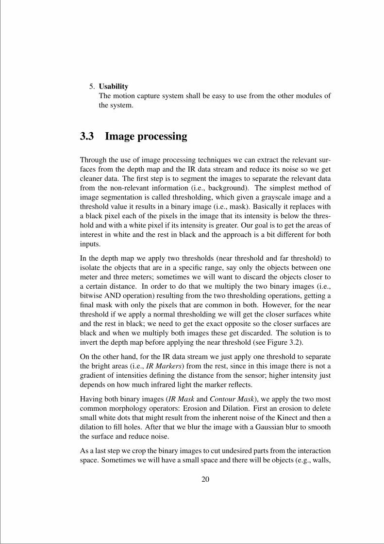
Through the use of image processing techniques we can extract the relevant sur-faces from the depth map and the IR data stream and reduce its noise so we getcleaner data. The first step is to segment the images to separate the relevant datafrom the non-relevant information (i.e., background). The simplest method ofimage segmentation is called thresholding, which given a grayscale image and athreshold value it results in a binary image (i.e., mask). Basically it replaces witha black pixel each of the pixels in the image that its intensity is below the thres-hold and with a white pixel if its intensity is greater. Our goal is to get the areas ofinterest in white and the rest in black and the approach is a bit different for bothinputs.

In the depth map we apply two thresholds (near threshold and far threshold) toisolate the objects that are in a specific range, say only the objects between onemeter and three meters; sometimes we will want to discard the objects closer toa certain distance. In order to do that we multiply the two binary images (i.e.,bitwise AND operation) resulting from the two thresholding operations, getting afinal mask with only the pixels that are common in both. However, for the nearthreshold if we apply a normal thresholding we will get the closer surfaces whiteand the rest in black; we need to get the exact opposite so the closer surfaces areblack and when we multiply both images these get discarded. The solution is toinvert the depth map before applying the near threshold (see Figure 3.2).

On the other hand, for the IR data stream we just apply one threshold to separatethe bright areas (i.e., IR Markers) from the rest, since in this image there is not agradient of intensities defining the distance from the sensor; higher intensity justdepends on how much infrared light the marker reflects.

Having both binary images (IR Mask and Contour Mask), we apply the two mostcommon morphology operators: Erosion and Dilation. First an erosion to deletesmall white dots that might result from the inherent noise of the Kinect and then adilation to fill holes. After that we blur the image with a Gaussian blur to smooththe surface and reduce noise.

As a last step we crop the binary images to cut undesired parts from the interactionspace. Sometimes we will have a small space and there will be objects (e.g., walls,

20

“main” — 2015/7/9 — 12:18 — page 21 — #35

Figure 3.2: Steps to get the contour from IR Data Stream and Depth Map.

floor, ceiling, furniture) that we do not want the system to track or bright lightsin the scene emitting infrared light that disturb the depth sensor and creates noise.These undesired areas can be blacken out so they do not affect the interaction bycropping the image, although the interaction space will be smaller. The processfor cropping is really simple: (1) create a mask of the same size as the image wewant to crop (640 × 480 pixels), (2) assign 0’s to the pixels we want to crop and1’s to the rest and (3) multiply the image by this mask.

All these image processing operations are done using the OpenCV library throughthe ofxCv addon and they are summarized in Figure 3.2.

3.4 Contour Detection

Having the two binary images from the previous step (IR Mask and ContourMask), we apply a contour detection algorithm to get the set of points definingthe boundary of all the white pixels in the image, namely the silhouette and IRMarkers boundaries. This technique is known as border following or contourtracing and the algorithm OpenCV uses is [Suzuki and Abe, 1985].

Given a binary image, the algorithm applies a raster scan and it interrupts the scanwhenever a pixel (i, j) satisfies one of the conditions in Figure 3.3. When this

21

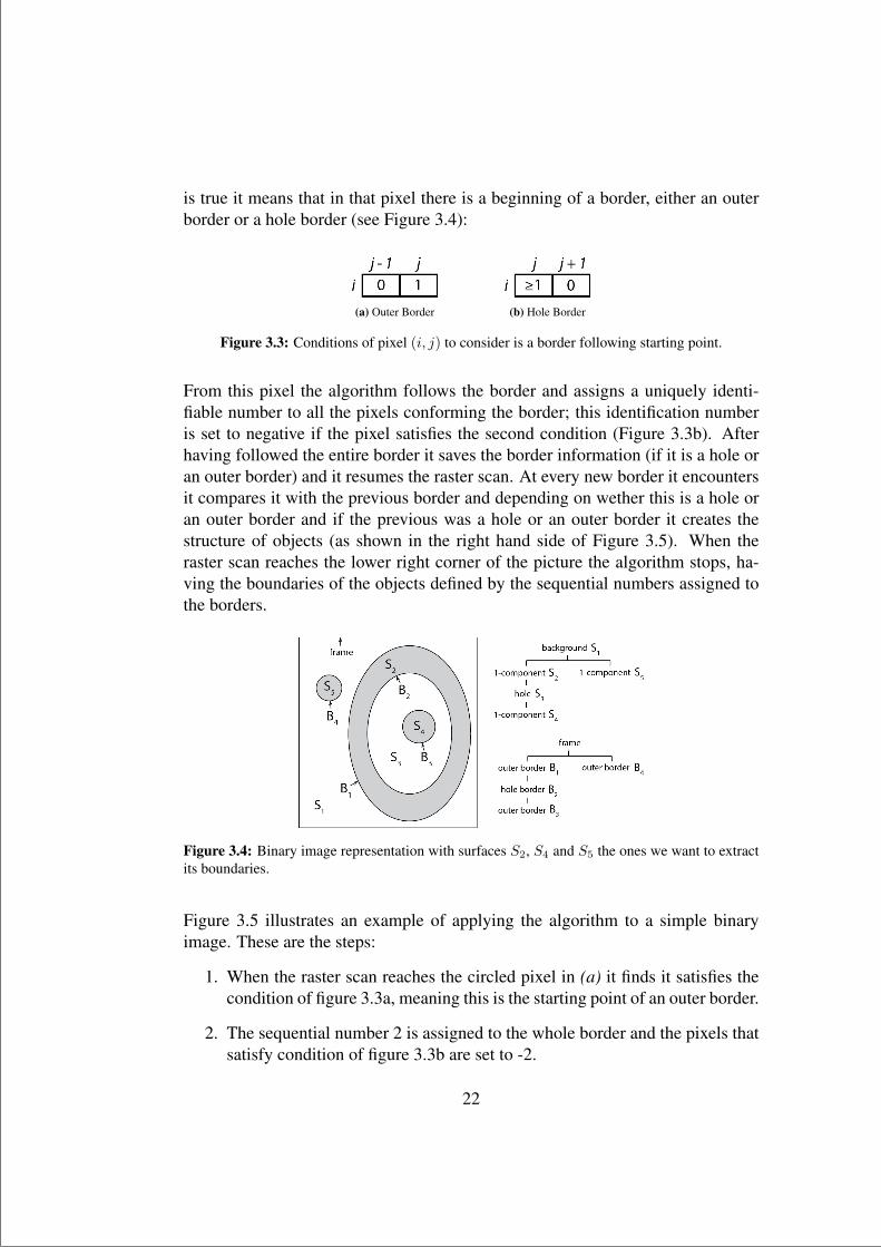
“main” — 2015/7/9 — 12:18 — page 22 — #36

is true it means that in that pixel there is a beginning of a border, either an outerborder or a hole border (see Figure 3.4):

(a) Outer Border (b) Hole Border

Figure 3.3: Conditions of pixel (i, j) to consider is a border following starting point.

From this pixel the algorithm follows the border and assigns a uniquely identi-fiable number to all the pixels conforming the border; this identification numberis set to negative if the pixel satisfies the second condition (Figure 3.3b). Afterhaving followed the entire border it saves the border information (if it is a hole oran outer border) and it resumes the raster scan. At every new border it encountersit compares it with the previous border and depending on wether this is a hole oran outer border and if the previous was a hole or an outer border it creates thestructure of objects (as shown in the right hand side of Figure 3.5). When theraster scan reaches the lower right corner of the picture the algorithm stops, ha-ving the boundaries of the objects defined by the sequential numbers assigned tothe borders.

Figure 3.4: Binary image representation with surfaces S2, S4 and S5 the ones we want to extractits boundaries.

Figure 3.5 illustrates an example of applying the algorithm to a simple binaryimage. These are the steps:

1. When the raster scan reaches the circled pixel in (a) it finds it satisfies thecondition of figure 3.3a, meaning this is the starting point of an outer border.

2. The sequential number 2 is assigned to the whole border and the pixels thatsatisfy condition of figure 3.3b are set to -2.

22

“main” — 2015/7/9 — 12:18 — page 23 — #37

Figure 3.5: Illustration of the process of extracting the contour from a binary image. The circledpixels are the starting points of border following.

3. By comparing this border with the latest encountered border (i.e., frame)we find out that its parent border is frame.

4. The raster scan is resumed and it gets interrupted by the circled pixel in (b),which satisfies condition of a hole border (figure 3.3b).

5. The border is followed and we assign the sequential number 3 or -3 in thesame manner as before.

6. Since this new border is a hole border and the previous encountered borderwas an outer border, we find out that this is his parent border.

7. Resuming the raster scan this does not get interrupted until the circled pixelin (c), which we find out is an outer border of a different object.

8. The algorithm ends when it scans the bottom-right pixel.

Applying this algorithm to the binary images we get the set of points conformingthe silhouette of the user (i.e., silhouette contour) and the area of the IR Markers(see Figure 3.2). By getting the centroid of the set of points conforming the IRMarkers (average position of all the points) we get a unique point describing theposition of the marker, which we later use to track its position over time.

23

“main” — 2015/7/9 — 12:18 — page 24 — #38

3.5 Tracking

In order to track the position of the markers over time we apply a simple trackingalgorithm that comes with the ofxCv addon. Having a list of the positions of themarkers in the actual frame and a list of the positions in the previous frame, thealgorithm finds the best match by comparing all the distances between them. Toidentify each of the markers in the list it assigns a uniquely identifying numberas a label. If there are more markers in the actual frame than in the previous,it creates new labels for them. On the other hand, if there are less markers inthe actual frame than in the previous the algorithm assigns the marker labels thatresult in the best match and the ones that remain unmatched start a counter of thenumber of frames that have been unmatched and are stored in a special vectorof ‘dead’ labels. In the following frames the actual markers positions are alsocompared with these unmatched labels positions and if they are closer than theother options, they get assigned to the marker; the counter is put to zero again andthe label is deleted from the ‘dead’ vector. If the counter surpasses a specifiedvalue (‘persistence’), the label is deleted from the list of possible marker labelsand is put in the vector of ‘dead’ labels forever.

One important value of this tracking algorithm is ‘maximumDistance’, which de-termines how far a marker can move until the tracker considers it a new one. Thisis done by filtering the different distances between the markers at every frame,eliminating those that are higher than ‘maximumDistance’.

In terms of the implementation we create anN×M matrix, whereN is the numberof markers in the actual frame and M the number of markers in the previousframe, containing the distances (filtered with ‘maximumDistance’) between all themarkers. Each row of the matrix is then sorted by distance and iterating through allthe rows we obtain the best match for each of the markers. For all the unmatchedmarkers from the actual frame (rows not assigned to any column) we assign a newidentifying label. In contrast, the unmatched markers from the previous frame(columns not assigned to any row) are put to the ‘dead’ vector and depending ifthey are young (counter is less than ‘persistence’) we just increment their counteror they are deleted from the list of previous markers (its corresponding column inthe matrix is deleted). As a last step, the position of the marker is interpolated withits previous position so we get a smoother movement between frames. Having thesequence of positions of the markers over time, it is really simple to get theirvelocity: subtract the position from the previous frame to the actual.

This tracking algorithm is not very robust and if the paths of the IR Markers getcrossed quickly its labels might swap. However, we can tolerate this error for thepurpose of our application.

24

“main” — 2015/7/9 — 12:18 — page 25 — #39

3.6 Optical Flow

Optical flow is defined as the pattern of apparent motion of objects by the relativemotion between an observer (in this case the Kinect sensor) and the scene. Thereare a many different methods to estimate this motion but the basic idea is to givena set of points in an image/frame find those same points in another image/frame.At the end we get a vector field describing the motion of all the single points fromthe first frame to the second. This approach fits perfectly in order to estimate themotion from the silhouette contours over time.

Following this idea we first implemented a very straightforward method using thesilhouette contour; for each point of the silhouette in the actual frame we computethe distance with every other point in the previous frame and we take the onethat is closest. By subtracting both points we estimate the velocity vector in thatposition. We end up with a set of vectors around the silhouette contour describingthe change of position from one frame to the other. This approach is implementedin CREA and it works but it is not being used; the estimation of the optical flowfulfills the same requirements with better results.

The methods to estimate the optical flow are normally classified in two differenttypes: dense techniques and sparse techniques. The former gives the flow estima-tion for all the pixels in the image while the latter only tracks a few pixels fromspecific features (e.g., object edges, corners and other structures well localized inthe image). Dense techniques are slower and are not good for large displacementsbut they can give more accuracy in the overall motion. For the purpose of CREAwe decided it was better to use a dense method since we wanted to get flow in-formation on the whole interaction area, which sparse techniques do not providesince it only tracks specific features.

Having said that, we decided to use the optical flow dense estimation methodprovided by OpenCV, Gunner Farneback’s Optical Flow [Farneback, 2003]. Theproblem with this approach was that the latest stable version of openFrameworks(0.8.4), which is the one used for this project, comes with an older OpenCV ver-sion (2.3.1) that does not support GPU computational capabilities, having to esti-mate the optical flow entirely using the CPU. As a result, in order to estimate theoptical flow in real-time we had to scale down the depth image and compute theflow on this lower resolution image. With this approach we were getting a decentframerate and the interaction with the graphics generated was very good for a fewhundred particles.

Once after we started adding graphics more computationally expensive to the sys-tem (e.g., fluid solver in section 4.3) we realized that the computation of the opti-

25

“main” — 2015/7/9 — 12:18 — page 26 — #40

cal flow was consuming most of the CPU, making the application work very slowwhen running everything together. As a solution, we started looking for opticalflow implementations based on the GPU. One of the options was to built the latestOpenCV version (which does already include optical flow GPU support), link itwith openFrameworks and make direct calls to the library. However, we foundout that the ofxFlowTools addon mentioned in Chapter 2 already implemented anoptical flow working in the GPU, making it easier to install for other users thatwould like to extend CREA and a cleaner code than the other approach.

This implementation uses a gradient-based method, which also provides a denseoptical flow. This method assumes that the brightness of any point in the imageremains constant (or changes very slowly) to estimate the image flow at everyposition in the image. Since we are using the binary depth image as input to theoptical flow and this has constant brightness throughout all the frames, this fitsvery well. This assumption of constant brightness can be written mathematicallyas:

I(~x, t) = I(~x+ ~u, t+ 1) (3.1)

Where I(~x, t) is the intensity of the image as a function of space ~x and time t and~u is the flow velocity we want to estimate.

By means of a Taylor series about ~x we can expand equation 3.1 and ignoring allthe terms higher than first order we get this equation:

∇I(~x, t) · ~u+ It(~x, t) = 0 (3.2)

Where∇I(~x, t) and It(~x, t) are the spatial gradient and the partial derivative withrespect to t of the image I , and ~u is the two dimensional optical flow vector.

Due to its nature, whenever we cannot estimate It(~x, t) we can replace it by com-puting the difference of I in two consecutive frames:

It(~x, t) ≡ I(~x, t+ 1)− I(~x, t) (3.3)

Given this, the implementation of a gradient-based optical flow is quite straight-forward. Since the computation is identical for every point in the space we cantake advantage of the parallelism of the GPU to estimate the velocity simultane-ously for every pixel. The implementation we use does that by calling a fragmentshader written in GLSL (OpenGL Shading Language) with the texture of the ac-tual frame (I(~x, t)) and the one in the previous (I(~x, t − 1)) as arguments. By

26

“main” — 2015/7/9 — 12:18 — page 27 — #41

(a) Optical Flow texture (b) Optical Flow velocity vectors

Figure 3.6: Optical Flow vector field texture with its corresponding velocity vectors representa-tion.

solving equation 3.2 it estimates the flow velocity for every pixel and stores thisinformation in another texture (the magnitude in ’x’ is stored in the red channeland the magnitude in ’y’ in the green channel, see Figure 3.6).

On top of that, this implementation includes another shader to blur the velocityfield temporally and spatially. To blur temporally it aggregates the flow textures atevery frame in one same buffer, slowly erasing the buffer by drawing a rectangleof the same size of the textures with a certain opacity. If this rectangle is drawnwith maximum opacity the buffer gets deleted at every frame and there is not anytemporal blur (the buffer only contains the actual flow texture). The opacity of thisrectangle is directly proportional to a ‘decay’ value; if ‘decay’ is high the opacityis high too and there is no temporal blur. In order to blur spatially, it applies aweighted average on each vector of the flow field texture with its neighbors, beingable to set the amount of blur by setting how many neighbors to use to computethe average (’radius’).

Although this algorithm runs very fast, since there is no need to have much pre-cision on the flow field for our purposes, we decided to use the same approachas we had done previously for the optical flow based on the CPU. The opticalflow is estimated using a lower resolution of the depth image (image scaled downby four). This makes the algorithm run faster and saves resources for computingmore complex graphics.

3.7 Velocity Mask

The velocity mask is an image that contains the areas where there has been mo-tion by using the optical flow field. Given an input image it returns this same

27

“main” — 2015/7/9 — 12:18 — page 28 — #42

image with only the pixels which position in the flow field correspond to a highvelocity.

The approach is quite simple and it is implemented using a fragment shader exe-cuted on the GPU, which means that for every pixel in the screen it does an inde-pendent operation. Using the optical flow texture (see Figure 3.6a) what we do isset a higher opacity in the input image pixel as higher the velocity is in that samepixel position in the flow texture. Basically we take the pixel value in the inputimage, take the same pixel in the flow texture (i.e., velocity) and set the magnitudeof this second pixel (i.e., magnitude of the velocity) as the opacity of the first. Thisresults in an image revealing the original pixels of the input image (higher opacitythan the rest) where there is motion.

This algorithm is really similar in concept as getting the absolute difference oftwo consecutive frames, which also results in the areas where there has been achange highlighted. However, with the velocity mask we have more control overthe motion areas by controlling the optical flow parameters and the result is moreprecise than just taking the frame difference (see Figure 3.7).

(a) Absolute Difference (b) Absolute Difference Contour Detection

(c) Velocity Mask (d) Velocity Mask Contour Detection

Figure 3.7: Difference in the result of applying a contour detection algorithm to the absolutedifference between two consecutive frames and using the velocity mask algorithm.

Having these areas of motion highlighted we can then apply the contour detectionalgorithm explained in section 3.4 to get the set of contour points defining theseregions (see Figure 3.7); we call them motion contours.

28

“main” — 2015/7/9 — 12:18 — page 29 — #43

3.8 Conclusions

In this chapter we have described our work on motion capture, covering all thealgorithms that have been used in the CREA system.

The algorithms used for motion capture work very well in most of the environ-ments and the latency is low enough for the purpose of this project. Moreover, theoutput data we obtain is quite precise and describes pretty accurately the motion ofthe performers, offering a great variety of possibilities for generating graphics thatrespond to this data. Having said that, we consider we have fulfilled satisfactorilythe proposed requirements from the beginning of the chapter.

The main problem of the motion capture is due to the inherent technology Mi-crosoft Kinect uses for getting the depth map. The depth map has quite a lotof noise/jitter and makes the algorithms that are based on this data slightly lessrobust. Sometimes this problem will be caused by infrared emitting lights in thevisual field that interfere with the depth sensor. One simple way to reduce this pro-blem is by using infrared filters/glass materials that filters/reflects outside the in-frared lights and lowers the interference with the depth sensor. [Camplani et al., 2013]proposes a more complex solution to this problem. By using spatial and temporalinformation from the depth map it obtains the missing values in the noisy areasand creates smoother edges and more homogeneous regions. This results in amore stable depth map with less jittering.

On the other hand, the new version of the Microsoft Kinect has been alreadyreleased and it is way more accurate and precise than the previous model. Thedepth sensor is more stable with interference of infrared lights and it has betterresolution on the depth map and infrared data stream. The drivers for this newsensor are still in a development phase and there are still several issues that haveto be fixed. Moreover, it only supports Microsoft Windows. As a result, thissolution it is not yet very practicable in the context of this project at the time wewrite this document but it is something to bear in mind in the very near future.Besides this, there are a large number of dedicated cameras that can be used toimprove the accuracy of the motion capture1.

In addition, there are other more precise motion capture techniques (see section2.1) that can provide with accurate skeletal data from the performers. This infor-mation would allow us to create particular graphics that respond better to the hu-man pose and to specific motions. This could also be achieved through the use ofthe EyeCon and EyesWeb technologies mentioned in section 2.3. [Piana et al., 2014]describes various ways of extracting features from body movements and recog-

1http://www.creativeapplications.net/tutorials/guide-to-camera-types-for-interactive-installations/

29

“main” — 2015/7/9 — 12:18 — page 30 — #44

nition of emotions in real-time using optical motion capture, which are used inEyesWeb.

30

“main” — 2015/7/9 — 12:18 — page 31 — #45

Chapter 4

GENERATION OF GRAPHICS INREAL-TIME

This chapter explains the algorithms used for generating the real-time graphicsbased on the data from the motion capture. First it introduces the problem ofgraphics generation and the list of functional and non-functional requirements thatwas considered from this part of the system. Next it describes briefly the mathsbehind the algorithms and how they are used inside CREA. The chapter ends upwith a short conclusion.

4.1 Introduction

There are many different algorithms and methods to generate interactive graphics.The idea from the very beginning was to focus on two-dimensional abstract andminimalistic graphics, using basic geometric elements such as lines and circles,that would simulate different behaviors based on the motion capture data. Many ofthe ideas for the graphics come from the projects mentioned in Chapter 2 and wetried to imitate some of their characteristics. Given that most of them use particlesystems to create various effects we decided to focus on this graphic technique,providing several features that would simulate different behaviors.

We also decided to implement a two-dimensional fluid solver on top of the particlesystems after a couple of projects1,2 from the digital artist Memo Atken. Thesimulation of realistic animations based on physical models such as fluids, are

1http://www.memo.tv/reincarnation/2http://www.memo.tv/waves/

31

“main” — 2015/7/9 — 12:18 — page 32 — #46

things that are already very beautiful to see just by themselves. Given the fact thatthe motion capture used is not very robust and has noise, creating graphics thatdo not need constant nor precise motion data input to look beautiful is a reallyimportant concept. Besides that, the fluid solver can also be used as an interactionmedium with the other graphics, enriching the system by creating a very naturaldialogue with the dancer.

Figure 4.1 summarizes the functionality of this part of the system and the sectionsexplained in this chapter. The output data from the motion capture (i.e., silhouettecontour, optical flow vector field, IR Markers position, IR Markers velocity...) isfed to the three graphical generation blocks: (1) Fluid Simulation, (2) ParticlesSystem Generation and (3) Silhouette Representation. In a step in between theMotion Capture and the graphics generation blocks the motion data is used as aninput to a two dimensional Fluid Solver. This solver outputs the fluid behaviordata over time which is then used as an extra input to the graphical generationblocks; being able to use it to interact with the graphics in a very organic andnatural way. The Fluid Solver and Fluid Simulation are very related and this iswhy we explain them together in the same section.

VideoProjector

Video image

Silhouette Representation

SilhouetteConvex hull

Bounding box

Fluid Solver

ParticlesSystem Generation

Emitter particlesGrid particles

Boids particlesAnimation particles

Fluid particles

FluidSimulation

Motion Capture

Figure 4.1: Block diagram of the graphics generation part of the system.

32

“main” — 2015/7/9 — 12:18 — page 33 — #47

4.2 Requirements

Following what we have mentioned in the introduction with respect to the gra-phics, we created the list of functionalities that the graphics generation modulewould have to accomplish and the constrains in order to satisfy the proper func-tioning of the overall system in the proposed context. First we explain the func-tional requirements and then we continue with the non-functional ones.

4.2.1 Functional Requirements

The list of functional requirements that we defined for the graphics generationsystem is the following:

1. Use motion captureThe graphics generation system must use the motion capture data as inputto the graphics generation algorithms. The graphics must interact with themotion data and also use it as a generating source.

2. Fluid SolverThe graphics generation system must include a two-dimensional fluid solverthat uses the motion capture data as control input. This fluid solver must beaccessible from the other graphic generation techniques in order to use thatas a way to create fluid behaviors.

3. Fluid SimulationThe graphics generation system must use the fluid solver as an input tosimulate fluid looking graphics, such as water and fire.

4. Particle SystemsThe graphics generation system must create particles with different beha-viors. These particles must follow a set of defined rules so they behave asa single system. The particles must simulate effects such as flocking, rain,snow and explosion animations.

5. User representationThe graphics generation system must represent in a few different ways thesilhouette of the user extracted from the motion capture.

33

“main” — 2015/7/9 — 12:18 — page 34 — #48

4.2.2 Non-functional Requirements

The list of non-functional requirements we defined for the graphics generationsystem is the following:

1. Fault ToleranceThe graphics generation system shall be tolerant to the noise coming fromthe motion capture data.

2. Real-timeThe graphics generation system shall guarantee response within 15 millise-conds from the input data.

3. Crash recoveryThe graphics generation system shall be able to restart in case of an unex-pected error in the generation algorithms.

4. ExtinsibilityThe graphics generation system shall take future growth into considerationand be easy to extend its functionalities.

4.3 Fluid Solver and Simulation

In order to implement a fluid solver we started reading a number of references oncomputer simulation of fluid dynamics and on different types of implementations([Harris, 2004], [Stam, 1999], [Stam, 2003], [West, 2008] and [Rideout, 2010]).Meanwhile we also learned about the basics of the OpenGL Shading Language([Rost and Licea-Kane, 2009], [Karluk et al., 2013] and [Vivo, 2015]) in order tounderstand how to program the fluid solver using the GPU capabilities. How-ever, after some time learning about fluids we discovered that two addons foropenFrameworks already implemented a two-dimensional fluid simulation. Theseaddons are already really optimized so we decided to use them instead of repro-gramming everything.

These two addons are: (1) ofxFluid3 and (2) ofxFlowTools4. First we started using(1) for its simplicity (only 2 files compared to 47 from (2)) but after some timeadapting it to the system we realized we were constantly checking (2) code as areference, so we decided to try (2). This implements an optical flow written inGLSL (see section 3.6), it has way more flexibility on the fluid parameters and

3https://github.com/patriciogonzalezvivo/ofxFluid4https://github.com/moostrik/ofxFlowTools

34

“main” — 2015/7/9 — 12:18 — page 35 — #49

ready to use features to use a live camera input to interact with the fluid. The op-erating principle and approach is the same in both, they are based on [Stam, 1999]method, which is not accurate enough for most engineering applications but it isideal for interactive computer graphical applications. This method is explained inthe following section.

4.3.1 Theory

To simulate the behavior of a fluid we need to get a mathematical representationof the state of the fluid at any given time. The most important quantity is the ve-locity, because it determines how the fluid and the objects inside the fluid move;we express the velocity over time as a vector field (i.e., velocity vector for everypoint in space) at each time step. There are many different models that have beendeveloped to simulate the fluid dynamics but the model we use is based on theNavier-Stokes equations, which is by far the most used equations among all theactual fluid solvers. We won’t explain the physics behind these equations sincethey are quite complex and there are many sources that already explain them re-ally well, we will just try to explain briefly what they say. Two excellent booksto introduce and understand the fundamental concepts of computational fluid dy-namics are [Chorin and Marsden, 2000] and [Abbott, 1997].

The basic idea is to determine the velocity field at each time step by solving aset of equations that describe the evolution of a fluid under a variety of forces.These set of equations are the Navier-Stokes equations, which given a velocityfield u and a scalar pressure field p for the initial time, they describe how the fluidchanges over time:

∇ · u = 0 (4.1)∂u

∂t= −(u · ∇)u− 1

ρ∇p− ν∇2u + F (4.2)

Where ν is the kinematic viscosity of the fluid, ρ is its density and F englobes allthe external forces acting on the fluid.

These equations come from assuming that the fluid is incompressible, whichmeans that the density of any subregion of the fluid doesn’t change during itsmotion through space. The equivalent of this is that the divergence of the flowvelocity is zero, which is what equation 4.1 says.

Using a mathematical result known as Helmholtz-Hodge Decomposition5 we can5http://en.wikipedia.org/wiki/Projection method (fluid dynamics)

35

“main” — 2015/7/9 — 12:18 — page 36 — #50

derive equations 4.1 and 4.2 to a single equation that is easier to solve, withoutthe pressure p term:

∂u

∂t= P(−(u · ∇)u+ ν∇2u + F ) (4.3)

Where P is called the projection operator and it is used to project a vector fieldonto a divergence free vector field that satisfies the incompressibility of the fluid(divergence zero at all points in the field∇ · u = 0).

Equation 4.3 is solved by sequentially solving each of the terms inside the paren-thesis on the right hand side: (1) advect6 the field and transport the velocities andother quantities around the space (−(u · ∇)u), (2) diffuse the field due to the vis-cous friction within the fluid (ν∇2u), (3) add all the external forces applied tothe fluid (F ) and (4) force the velocity to conserve mass applying the projectionoperator (P). The details on how to solve each of these steps numerically andhow to apply the projection operator is described precisely in [Stam, 1999] and[Harris, 2004].

On top of this there are other terms that can be added in the function to extendthe features of the fluid simulation, such as (1) buoyancy and (2) vorticity con-finement. Buoyancy is the force that acts on the fluid due to the changes of tem-perature. We simply need to add a new scalar field (i.e., temperature) that adds aforce where the local temperature is higher than the given ambient temperature.Vorticity is a measure of spinning and rotation of the fluid and vorticity confine-ment what makes the fluid preserve better this rotation over time. This is doneby measuring where vorticity is being lost and injecting rotational motion in theseareas so they keep spinning longer.

4.3.2 Implementation

In terms of the implementation there is a two-dimensional grid of cells storing dif-ferent data types that describe the state of the fluid (e.g., velocity vector, density,pressure, temperature, vorticity and any other substances that we want to prop-agate with the fluid flow). The process is to keep solving the equations for thedifferent substances at each time step and update the values of the cells.

If this was implemented using the CPU there would be a pair of nested loopsiterating over each cell in the grid to perform the same computation over and overand update its values. However, since the operations at each cell are identical,we can take advantage of the parallelism of the GPU and do these computations

6http://en.wikipedia.org/wiki/Advection

36

“main” — 2015/7/9 — 12:18 — page 37 — #51

simultaneously; instead of using grids of cells we use textures that store the data inits pixels (e.g., the ‘x’ magnitude of the velocity can be stored in the red channel,the ‘y’ magnitude in the green channel and the blue and alpha channels can beused to store the temperature or any other pressure scalar, see Figure 4.2) and runfragment shaders to update its values. For each of the steps that solve equation4.3 and that we have explained in the previous section there is a fragment shaderthat solves the equation in the specific pixel. The code of these fragment shadersis simply the transcription of the mathematical formulas (see [Harris, 2004] formore details). The two most important textures to represent the state of the fluidare the fluid velocity (see Figure 4.2a) and the scalar pressure field (see Figure4.2b).

To draw a simulation of the fluid we just need to draw the texture containing thecolor density carried by the fluid (see Figure 4.3d and Figure 4.4d) but we canuse any of the other textures to do anything we can imagine (e.g., use the velocityfield to move objects, draw the velocity vector field as a grid of vectors, use thetemperature texture to draw smoke densities).

(a) Velocity (b) Pressure (c) Temperature (d) Vorticity

Figure 4.2: State fields of the fluid simulation stored in textures.

The behavior of the fluid can be controlled by altering the values of the state fieldtextures. This is done by creating new textures and summing them to the fluidstate textures before solving the equations. As an example, if we create a texturewith a pixel in the red channel with value 100 and the rest to 0 and we sum it tothe velocity state field texture (see Figure 4.2a), the solver will interpret this as anhorizontal force of magnitude 100 being applied in that pixel position. We havecreated two different methods to control the behavior of the fluid, one using thesilhouette contour data and the other using the IR Markers.

Silhouette Contour Input

Uses the motion capture data that comes from the depth map to control the fluid.To change the acceleration of the velocity field of the fluid we use the optical flowtexture (see Figure 4.3a); summing the pixel values of this texture to the fluid

37

“main” — 2015/7/9 — 12:18 — page 38 — #52

velocity field (see Figure 4.2a) and multiplying the former by a scalar to controlhow much it effects to the flow.

To add density to the fluid we sum the velocity mask (see section 3.7) to the fluiddensity texture (see Figure 4.3d), adding density only the areas where there ismotion. This density is the one that defines the color of the fluid and since thevelocity mask is white by default, our hack was to tint the binary depth imagewith the desired color before using it to compute the velocity mask (see Figure4.3b). To tint the image we use a framebuffer7 and below there is the code thatdoes that, with an extra method that changes the color randomly over time usingPerlin Noise:

1 / / t i n t b i n a r y d e p t h image ( s i l h o u e t t e )2 co lo r edDe p thFbo . b e g i n ( ) ; / / s t a r t t o draw i n t h e f r a m e b u f f e r3 o f P u s h S t y l e ( ) ;4 o f C l e a r ( 2 5 5 , 255 , 255 , 0 ) ; / / c l e a r b u f f e r5 i f ( vMaskRandomColor ) { / / t i n t image wi th random c o l o r s u s i n g p e r l i n n o i s e6 vMaskColor . s e t Hs b ( ofMap ( o f N o i s e ( o f G e t E l a p s e d T i m e f ( ) ∗0 . 3 ) , 0 . 1 , 0 . 9 , 0 , 255 ,

t r u e ) , 255 , 255) ;7 vMaskRed = vMaskColor . r ;8 vMaskGreen = vMaskColor . g ;9 vMaskBlue = vMaskColor . b ;

10 }11 / / t i n t image wi th s p e c i f i e d c o l o r12 vMaskColor . s e t ( vMaskRed , vMaskGreen , vMaskBlue , vMaskOpaci ty ) ;13 o f S e t C o l o r ( vMaskColor ) ; / / s e t draw c o l o r14 dep thImage . draw ( 0 , 0 , width , h e i g h t ) ; / / draw b i n a r y image i n t h e b u f f e r15 o f P o p S t y l e ( ) ;16 co lo r edDe p thFbo . end ( ) ;

Finally we also inject temperature in the areas of motion by using the luminancechannel from the velocity mask texture (see Figure 4.3c), being the pixel intensi-ties the temperature in that area. This generates buoyancy due to the differencesin temperature.

(a) Optical Flow (b) Density (c) Temperature (d) Density State Field

Figure 4.3: Silhouette Contour Input textures for the Fluid Solver and density state field texture.

7http://openframeworks.cc/documentation/gl/ofFbo.html

38

“main” — 2015/7/9 — 12:18 — page 39 — #53

IR Markers Input

Uses the data from the IR Markers to control the fluid by using a very similarprocedure as the one described for the Silhouette Contour Input. To change theacceleration of the fluid flow we use the velocity of the marker; creating a texturewith circles in the IR Markers positions encoding the velocity data (i.e., the redchannel contains the magnitude in ‘x’ of the marker velocity and the green channelthe magnitude in ‘y’ ) and summing the texture to the fluid velocities texture. Thebigger the radius of the circles the largest the region that will be affected by themarker velocity (see Figure 4.4a).

For injecting color we follow the exact same idea but the circles are drawn withthe color we want to add to the density texture (see Figure 4.4b). By blurring theedges of the circles the injected density is more subtile and smooth.

Finally for injecting temperature and generating buoyancy we just draw the circleswith its color intensity as the desired temperature (see Figure 4.4c).

(a) Velocity (b) Density (c) Temperature (d) Density State Field

Figure 4.4: IR Markers Input textures for Fluid Solver and density state field texture.

4.4 Particle System Generation

A particle system is a really common technique in computer graphics that uses alarge number of independent objects to simulate different effects and behaviors.The idea is to be able to manage the number of particles in a flexible way (createand delete the particles) and update their attributes over time according to a set ofrules (e.g., gravity, friction, forces).

Chapter 3 of [Perevalov, 2013] and Chapter 4 of [Shiffman, 2012] describe how toimplement a basic particle system with some simple behavior functionalities.

First we explain how the equations that describe the motion of the particles arederived and how the class of a single particle was implemented from those equa-tions. Next we explain how the particle system class was implemented, which is

39

“main” — 2015/7/9 — 12:18 — page 40 — #54

the one that manages the particles and makes them behave as a single element;describing how the motion capture data is used to interact in different ways withthe particles. Finally we explain the five different particle system behaviors crea-ted: (1) Emitter particles, (2) Grid particles, (3) Boids particles, (4) Animationsparticles and (5) Fluids particles. Although these share the same basic structure,the set of rules that control the particles are very different and that is why they areexplained separately.

4.4.1 Theory

In order to describe the motion of a particle we need to save its position andvelocity and apply forces to adjust its acceleration. Given these attributes in thecurrent time step, the challenge is to know how to predict the values in the nexttime step. The formula that dictates the motion of objects is Newton’s secondlaw:

~F = m~a = m∂~v

∂t= m

∂2~x

∂t2(4.4)

Where ~F is the force, m is the mass, ~a is the acceleration, ~v is the velocity, ~x isthe position and t is time.

Knowing that the velocity is the derivative of acceleration and position the deriva-tive of velocity, we can separate Newton’s second law in two first order diffe-rential equations and solve them following Euler’s method. The solution is anapproximation of how position and velocity change over time given the actualvalues:

~v′ = ~v + ~a∆t (4.5)~x′ = ~x+ ~v∆t (4.6)

Where ~v′ is the new velocity, ~v is the actual velocity, ~a is the acceleration, ~x′is the new position, ~x the actual position and ∆t the time step (time betweenframes).

There are other methods to approximate the solution of differential equations thatare more precise (e.g., Verlet integration, Runge-Kutta method) but for the pur-pose of this system physical accuracy is secondary.

40

“main” — 2015/7/9 — 12:18 — page 41 — #55

4.4.2 Single Particle

Following the previous equations we can implement the basic functionality to des-cribe the motion of a single particle over time. The steps that we do at every frameare: (1) compute the acceleration of the particle by summing all the external forcesacting on it divided by its mass (Newton’s second law), (2) add the accelerationmultiplied by the time step to the velocity, (3) add the velocity multiplied bythe time step to the position and (4) restart the forces. In order to make thismotion more realistic we also add a ‘friction’ variable that makes the velocity ofthe particle decay. This variable ranges from 0.9 to 1.0 and multiplying it by thevelocity after summing the acceleration makes the particle slow down in a verynatural way:

1 acc = f r c / mass ; / / Newton ’ s second law F = m∗a2 v e l += acc∗ d t ; / / E u l e r ’ s method3 v e l ∗= f r i c t i o n ; / / Decay v e l o c i t y4 pos += v e l ∗ d t ;5 f r c . s e t ( 0 , 0 ) ; / / R e s t a r t f o r c e

In order to control the motion of the particle we have to apply external forces inthe direction we want the particle to move, changing its acceleration. The methodthat does that is the following:

1 vo id P a r t i c l e : : addForce ( o f P o i n t f o r c e ) {2 f r c += f o r c e ;3 }

Besides this, we decided it would be helpful to have a couple of methods more tomake the particle attract to or repulse from a specific source point. The methodthat adds a repulsion force from a point is the following:

1 vo id P a r t i c l e : : a d d R e p u l s i o n F o r c e ( o f P o i n t posOfForce , f l o a t r a d i u s S q r d , f l o a ts c a l e ) {

2

3 / / ( 1 ) c a l c u l a t e t h e d i r e c t i o n t o f o r c e s o u r c e and d i s t a n c e4 o f P o i n t d i r = pos − posOfForce ;5 f l o a t d i s t S q r d = pos . s q u a r e D i s t a n c e ( posOfForce ) ;6

7 / / ( 2 ) i f c l o s e enough u p d a t e f o r c e8 i f ( d i s t S q r d < r a d i u s S q r d ) {9 f l o a t p c t = 1 − ( d i s t S q r d / r a d i u s S q r d ) ; / / s t r o n g e r on t h e i n s i d e

10 d i r . n o r m a l i z e ( ) ;11 f r c += d i r ∗ s c a l e ∗ p c t ;12 }13 }

This method applies a repulsion force with magnitude ‘scale’ to the particle if thepoint ‘posOfForce’ is closer to a distance ‘radiusSqrd’. First we get the directionof the repulsion force (i.e., vector pointing from the point towards the particle),by subtracting the position of the point to the position of the particle. Then we

41

“main” — 2015/7/9 — 12:18 — page 42 — #56

compute the square distance between the force source and the particle and checkif this distance is smaller than the minimum repulsion distance. If the particleis close enough to the source of force, we get the ratio of this distance with theminimum repulsion distance (‘pct’) and multiply it by the direction (normalized)of the force and the strength of the repulsion force. This ratio makes the particlerepulse faster if it is closer to the repulsion point.

The attraction force method (‘addAttractionForce’) is exactly the same with theonly difference that the direction of the force is inverted.

The fact that we use the square distance and not the distance itself is that thesquare root calculation is much more processor-intensive than multiplying; theuse of square roots inside nested loops really makes the frame rate slow down.Due to this we use square distances and square lengths all the time throughout thecode.

We can extend the particle attributes adding as many variables as we want. Theseare some of the extra control variables that the particle class includes:

id Float number that uniquely identifies the particle.

iniPos Position of the particle when it borns.

age Time that the particle has lived.

lifetime How much time the particle will live.

radius Actual size of the particle.

iniRadius Radius of the particle when it borns.

color Color of the particle.

opacity Opacity of the particle.

With these extra variables we can have much more control on the behavior of theparticle over time. Make the particle decrease size throughout its lifespan, changeits color, opacity or make it return to its original position.

Another very useful function created was to add some randomness to the motionof the particle using Perlin noise8; this is a pseudo-random noise that creates asmoothly interpolated sequence of values that is very frequently used in computergraphics to simulate various organic effects. The great advantage of this noisefunction is that it can be defined in any dimension and it always gives a consistentvalue for a particular location, creating a very natural looking evolution of therandom values.

8http://en.wikipedia.org/wiki/Perlin noise

42

“main” — 2015/7/9 — 12:18 — page 43 — #57

This is the code of the function in question, which adds a random vector withmagnitude ‘turbulence’ to the external forces acting on the particle:

1 vo id P a r t i c l e : : addNoise ( f l o a t t u r b u l e n c e ) {2 / / P e r l i n n o i s e3 f l o a t a n g l e = o f S i g n e d N o i s e ( i d ∗0 .001 f , pos . x ∗ 0 .005 f , pos . y ∗ 0 .005 f ,

o f G e t E l a p s e d T i m e f ( ) ∗ 0 . 1 f ) ∗ 2 0 . 0 f ;4 o f P o i n t n o i s e V e c t o r ( cos ( a n g l e ) , s i n ( a n g l e ) ) ;5 i f ( ! im m o r t a l ) f r c += n o i s e V e c t o r ∗ t u r b u l e n c e ∗ age ; / / i f i m m o r t a l t h i s

doesn ’ t a f f e c t , age == 06 e l s e f r c += n o i s e V e c t o r ∗ t u r b u l e n c e ;7 }

Since the force is in two dimensions we need to get a vector also in two dimen-sions that can be summed to the force. In order to get that we treat the noise asan angle and get the ‘x’ and ‘y’ offset, which define the coordinates of a vectorthat smoothly changes over time. Having that we just multiply this vector by the‘turbulence’ variable, to control the amount of noise, and by the age of the particleso the effect increases as the particle gets older.

To compute the noise we use the ‘id’ of the particle, its current position and theelapsed time since the application started. By using the identifier ‘id’ we get aunique noise result for each particle and the elapsed time makes the noise functionoutput different values even when the particle rests in the same position, since theelapsed time increments gradually (if we give the same arguments to the Perlinnoise function it outputs the same value every time).

The ‘ofSignedNoise’ built-in noise function from openFrameworks outputs a valuebetween -1.0 and 1.0, having to multiply this by a scalar if we want this value torepresent an angle in the range of all the radians in a circle. The noise is multipliedby 20.0 and not by π because the output range does not result in an even distribu-tion (often the results stay betwen -0.25 and 0.25), thus the random motion of theparticles tend to favor a specific direction. By multiplying by 20.0 the angle rangeis greater and the distribution is more even.

4.4.3 Particle System

The particle system class manages the collection of particles and defines the setof rules we want the particles to follow over time. In order to do that it has adynamic vector with all the particles and various methods to update their attributesand define their behavior. There are many different behaviors that we can simulatewith particle systems but we decided to separate these in five different groups: (1)Emitter particles, (2) Grid particles, (3) Boids particles, (4) Animations particlesand (5) Fluid particles. First we explain the general features that these types havein common and next the particularities of each of the categories.

43

“main” — 2015/7/9 — 12:18 — page 44 — #58

The approach to make the particles interact is the same for the five groups butsome interactions are only meaningful for certain groups. The interaction caneither be between particles or from an input source (IR Markers and SilhouetteContour). The interactions we have implemented are: (1) Particle-particle repul-sion, (2) Particle-particle connection, (3) Flow interaction, (4) Fluid interaction,(5) Repulse interaction, (6) Attract interaction, (7) Seek interaction, (8) Gravityinteraction and (9) Bounce interaction.

When using the IR Markers as input, since there can be more than one markerbeing tracked, we need to have a way to make the particles decide which markerto interact with. As a result, we implemented a method to compute the closestmarker to the particle:

1 i r M a r k e r ∗ P a r t i c l e S y s t e m : : g e t C l o s e s t M a r k e r ( c o n s t P a r t i c l e &p a r t i c l e ,v e c t o r<i rMarke r> &markers , f l o a t i n t e r a c t i o n R a d i u s S q r d ) {

2

3 i r M a r k e r ∗ c l o s e s t M a r k e r = NULL;4 f l o a t minDi s tSq rd = i n t e r a c t i o n R a d i u s S q r d ;5

6 / / Get c l o s e s t marker t o p a r t i c l e7 f o r ( i n t marke r Index = 0 ; marke r Index < marke r s . s i z e ( ) ; marke r Index ++){8 i f ( ! marke r s [ marke r Index ] . h a s D i s a p p e a r e d ) {9 f l o a t m a r k e r D i s t S q r d =

p a r t i c l e . pos . s q u a r e D i s t a n c e ( marke r s [ marke r Index ] . smoothPos ) ;10 i f ( m a r k e r D i s t S q r d < minDis tSq rd ) {11 minDis tSq rd = m a r k e r D i s t S q r d ;12 c l o s e s t M a r k e r = &marke r s [ marke r Index ] ;13 }14 }15 }16

17 r e t u r n c l o s e s t M a r k e r ;18 }

Basically it computes the square distance between the particle position and thedifferent markers and returns a pointer to the closest if the particle is within theinteraction radius area of the marker. Having the pointer to the closest marker wecan apply any change of behavior we can think of based on the attributes stored inthe marker class (e.g., position and velocity of the marker).

For the Silhouette Contour we also need to get the closest point from the differentsilhouettes detected in the interaction space. The approach is very similar:

1 o f P o i n t P a r t i c l e S y s t e m : : g e t C l o s e s t P o i n t I n C o n t o u r ( c o n s t P a r t i c l e& p a r t i c l e , c o n s tContour& c o n t o u r , boo l o n l y I n s i d e , u n s i g n e d i n t ∗ c o n t o u r I d x ) {

2

3 o f P o i n t c l o s e s t P o i n t (−1 , −1) ;4 f l o a t minDi s tSq rd = 99999999;5

6 / / Get c l o s e s t p o i n t t o p a r t i c l e from t h e d i f f e r e n t c o n t o u r s7 f o r ( u n s i g n e d i n t i = 0 ; i < c o n t o u r . c o n t o u r s . s i z e ( ) ; i ++){8 i f ( ! o n l y I n s i d e | | c o n t o u r . c o n t o u r s [ i ] . i n s i d e ( p a r t i c l e . pos ) ) {9 o f P o i n t c a n d i d a t e P o i n t = c o n t o u r . c o n t o u r s [ i ] . g e t C l o s e s t P o i n t ( p a r t i c l e . pos ) ;

10 f l o a t p o i n t D i s t S q r d = p a r t i c l e . pos . s q u a r e D i s t a n c e ( c a n d i d a t e P o i n t ) ;

44

“main” — 2015/7/9 — 12:18 — page 45 — #59

11 i f ( p o i n t D i s t S q r d < minDis tSq rd ) {12 minDis tSq rd = p o i n t D i s t S q r d ;13 c l o s e s t P o i n t = c a n d i d a t e P o i n t ;14 i f ( c o n t o u r I d x != NULL) ∗ c o n t o u r I d x = i ; / / s ave c o n t o u r i n d e x15 }16 }17 }18

19 r e t u r n c l o s e s t P o i n t ;20 }

If the variable ‘onlyInside’ is equal to true the method returns the closest pointonly if the particle is inside the silhouette contour, being able to use this so weonly interact with the particles inside the silhouette. Otherwise if the variableis equal to false, it returns the closest point to the particle no matter where thisis. Moreover, the method also stores the index of the contour in the ‘contourIdx’pointer so we can use all the set of points conforming the silhouette contour tointeract with the particle (see Bounce Interaction).

Particle-particle repulsion

This adds a repulsion force to the particles when they get too close. The mostbasic implementation would be to add two loops that for every particle compareshow close is this one to all the others and applies a repulsion force if the distanceis smaller than a threshold:

1 vo id P a r t i c l e S y s t e m : : r e p u l s e P a r t i c l e s ( ) {2 f l o a t r e p u l s e D i s t S q r d = r e p u l s e D i s t ∗ r e p u l s e D i s t ;3 f o r ( i n t i = 0 ; i < p a r t i c l e s . s i z e ( ) ; i ++){4 f o r ( i n t j = 0 ; j < p a r t i c l e s . s i z e ( ) ; j ++){5 i f ( j != i ) p a r t i c l e s [ i ]−>a d d R e p u l s i o n F o r c e ( p a r t i c l e s [ j ] . pos ,

r e p u l s e D i s t S q r d , 3 0 . 0 ) ;6 }7 }8 }

The complexity of this approach is O(n2) since each particle is compared with allthe others, being really slow if we have a few hundreds of particles.

One improvement is to pass by reference the particle from where we apply therepulsion force and add the same force in the opposite direction also to this parti-cle. We created a modified version of the method ‘addRepulsionForce’ explainedbefore:

1 vo id P a r t i c l e : : a d d R e p u l s i o n F o r c e ( P a r t i c l e &p , f l o a t r a d i u s S q r d , f l o a t s c a l e ) {2

3 / / ( 1 ) make a v e c t o r o f where t h e p a r t i c l e p i s :4 o f P o i n t posOfForce ;5 posOfForce . s e t ( p . pos . x , p . pos . y ) ;6

45

“main” — 2015/7/9 — 12:18 — page 46 — #60

7 / / ( 2 ) c a l c u l a t e t h e d i r e c t i o n t o p a r t i c l e and d i s t a n c e8 o f P o i n t d i r = pos − posOfForce ;9 f l o a t d i s t S q r d = pos . s q u a r e D i s t a n c e ( posOfForce ) ;

10

11 / / ( 3 ) i f c l o s e enough u p d a t e bo th f o r c e s12 i f ( d i s t S q r d < r a d i u s S q r d ) {13 f l o a t p c t = 1 − ( d i s t S q r d / r a d i u s S q r d ) ; / / s t r o n g e r on t h e i n s i d e14 d i r . n o r m a l i z e ( ) ;15 f r c += d i r ∗ s c a l e ∗ p c t ;16 p . f r c −= d i r ∗ s c a l e ∗ p c t ;17 }18 }

Using this method we only need to do half of the iterations:1 vo id P a r t i c l e S y s t e m : : r e p u l s e P a r t i c l e s ( ) {2 f l o a t r e p u l s e D i s t S q r d = r e p u l s e D i s t ∗ r e p u l s e D i s t ;3 f o r ( i n t i = 1 ; i < p a r t i c l e s . s i z e ( ) ; i ++){4 f o r ( i n t j = 0 ; j < i ; j ++){5 p a r t i c l e s [ i ]−>a d d R e p u l s i o n F o r c e (∗ p a r t i c l e s [ j ] , r e p u l s e D i s t S q r d , 3 0 . 0 ) ;6 }7 }8 }

Another big improvement is to sort the vector of particles spatially at each iterationso we only check the particles that are close to each other. In this case we decidedto sort the vector by the ‘x’ coordinate, having the vector ordered by how theparticles appear from left to right in the space. Having the vector ordered weonly have to compare each particle with the ones that are within the horizontalrange of the minimum repulsion distance. Because of that, we start to comparethe particle with the one right next to it (j = i-1) and stop the loop when thedistance between them is greater than the minimum:

1 boo l c o m p a r i s o n F u n c t i o n ( P a r t i c l e ∗ a , P a r t i c l e ∗ b ) {2 r e t u r n a−>pos . x < b−>pos . x ;3 }4

5 s o r t ( p a r t i c l e s . b e g i n ( ) , p a r t i c l e s . end ( ) , c o m p a r i s o n F u n c t i o n ) ;6

7 vo id P a r t i c l e S y s t e m : : r e p u l s e P a r t i c l e s ( ) {8 f l o a t r e p u l s e D i s t S q r d = r e p u l s e D i s t ∗ r e p u l s e D i s t ;9 f o r ( i n t i = 1 ; i < p a r t i c l e s . s i z e ( ) ; i ++){

10 f o r ( i n t j = i −1; j >= 0 ; j−−){11 i f ( f a b s ( p a r t i c l e s [ i ]−>pos . x − p a r t i c l e s [ j ]−>pos . x ) > r e p u l s e D i s t ) {12 b r e a k ; / / s t o p second loop and jump t o n e x t p a r t i c l e13 }14 p a r t i c l e s [ i ]−>a d d R e p u l s i o n F o r c e ( ∗ p a r t i c l e s [ j ] , r e p u l s e D i s t S q r d , 3 0 . 0 ) ;15 }16 }17 }

There are better techniques to make this comparisons even more efficiently, allof them based on spatially organizing the particles so the comparisons are con-strained to the closer particles (see section 4.6).

46

“main” — 2015/7/9 — 12:18 — page 47 — #61

Particle-particle connection

This draws a line connecting the particles if they are closer than a certain distance.Basically it compares each particle with all the others and if they are closer than athreshold it draws a connecting line in between. In order to compare each particlewith the others efficiently we use the same technique described in Particle-particlerepulsion:

1 i f ( d r awConnec t i ons ) {2 o f P u s h S t y l e ( ) ;3 f l o a t c o n n e c t D i s t S q r d = c o n n e c t D i s t ∗ c o n n e c t D i s t ;4 o f S e t C o l o r ( o f C o l o r ( red , green , b l u e ) , o p a c i t y ) ;5 o f S e t L i n e W i d t h ( connec tWid th ) ;6 f o r ( i n t i = 0 ; i < p a r t i c l e s . s i z e ( ) ; i ++){7 f o r ( i n t j = i −1; j >= 0 ; j−−){8 i f ( f a b s ( p a r t i c l e s [ j ]−>pos . x − p a r t i c l e s [ i ]−>pos . x ) > c o n n e c t D i s t ) {9 b r e a k ; / / s t o p second loop and jump t o n e x t p a r t i c l e

10 }11 i f ( p a r t i c l e s [ i ]−>pos . s q u a r e D i s t a n c e ( p a r t i c l e s [ j ]−>pos ) < c o n n e c t D i s t S q r d ) {12 o f L i n e ( p a r t i c l e s [ i ]−>pos , p a r t i c l e s [ j ]−>pos ) ;13 }14 }15 }16 o f P o p S t y l e ( ) ;17 }

Flow Interaction

The approach for this interaction is different for the two possible inputs: SilhouetteContour and IR Markers.

For the case of the Silhouette Contour input this interaction is based on the outputof the optical flow vector field (see section 3.6), which is stored in a texture withthe red channel being the horizontal offset and the green channel the vertical. Theprinciple is to apply to every particle the velocity that corresponds to the sameposition in the flow field; adding this velocity as an external force that acts on theparticle. In order to do that we had to implement a method to get the velocitygiven the position of the particle.

Since for computing the optical flow we use a lower resolution image of the Kinectdepth map, the first step to get the velocity in a specific coordinate is to scale thecoordinate system down so the coordinates of the particles match the coordinatesof the optical flow texture. After that, we simply get the color of the texture in thatcoordinate and assign the red channel to the x coordinate and the green channel tothe y coordinate of the velocity vector:

1 ofVec2f Contour : : g e t F l o w O f f s e t ( o f P o i n t p ) {2 o f P o i n t p = p / s c a l e F a c t o r ; / / s c a l e p o i n t t o match f low t e x t u r e

47

“main” — 2015/7/9 — 12:18 — page 48 — #62

3 ofVec2f o f f s e t ( 0 , 0 ) ;4

5 i f ( r e s c a l e d R e c t . i n s i d e ( p ) ) { / / i f p o i n t i s i n s i d e f low t e x t u r e s i z e6 o f f s e t . x = f l o w P i x e l s [ ( ( i n t ) p . y∗ f lowWidth +( i n t ) p . x ) ∗3 + 0 ] ; / / r7 o f f s e t . y = f l o w P i x e l s [ ( ( i n t ) p . y∗ f lowWidth +( i n t ) p . x ) ∗3 + 1 ] ; / / g8 }9

10 r e t u r n o f f s e t ;11 }

The only secret of this function is how to read the pixels of the texture by its coor-dinates. Whenever we want to manipulate the pixel data of a texture (ofTexture),which resides in memory in the GPU, we first need to transfer the texture data tothe CPU (ofPixels), like we do here in this part of code:

1 o f F l o a t P i x e l s f l o w P i x e l s ;2 / / Save o p t i c a l f low t e x t u r e and g e t i t s p i x e l s t o r e a d v e l o c i t i e s3 o f T e x t u r e f l o w T e x t u r e = o p t i c a l F l o w . g e t O p t i c a l F l o w D e c a y ( ) ;4 f l o w T e x t u r e . r e a d T o P i x e l s ( f l o w P i x e l s ) ;

When we do this we are saving the texture as a one dimensional array of pixelvalues, storing each row of the texture next to each other. Hence, if we want toaccess the 10th pixel of the 2nd row of the texture we would simply multiply by2 the width of the texture and sum 10 (flowPixels[2*textureWidth+10]). Sincethe flow texture has three channels (RGB), for each pixel there are three values,stored one after the other in the array, having to multiply by 3 the previous resultto access the pixel in that coordinate. Then we just sum 1 or 2 to read the secondand third channel respectively.

The reason why we use ‘ofFloatPixels’ instead of ‘ofPixels’ is that the latter storesits values in 1 byte (unsigned char) and the former in 4 bytes (float) and the flowtexture data is also stored in 4 bytes. We explicitly mention this since it wasa common error in the code and it took us some time to realize what was theerror.

Having the velocity vector in the particle position we just apply it as an externalforce acting on the particle:

1 u n s i g n e d i n t c o n t o u r I d x = −1;2 o f P o i n t c l o s e s t P o i n t I n C o n t o u r ;3 i f ( p a r t i c l e M o d e == BOIDS && s e e k I n t e r a c t i o n ) c l o s e s t P o i n t I n C o n t o u r =

g e t C l o s e s t P o i n t I n C o n t o u r (∗ p a r t i c l e s [ i ] , c o n t o u r , f a l s e , &c o n t o u r I d x ) ;4 e l s e c l o s e s t P o i n t I n C o n t o u r = g e t C l o s e s t P o i n t I n C o n t o u r (∗ p a r t i c l e s [ i ] , c o n t o u r ,

t r u e , &c o n t o u r I d x ) ;5

6 i f ( f l o w I n t e r a c t i o n ) {7 o f P o i n t f r c = c o n t o u r . g e t F l o w O f f s e t ( p a r t i c l e s [ i ]−>pos ) ;8 p a r t i c l e s [ i ]−>addForce ( f r c ∗ i n t e r a c t i o n F o r c e ) ;9 }

For the case of IR Markers this interaction is based on the velocity of the marker.We simply get the velocity of the closest marker within the interaction area and

48

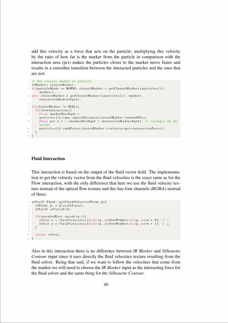
“main” — 2015/7/9 — 12:18 — page 49 — #63

add this velocity as a force that acts on the particle; multiplying this velocityby the ratio of how far is the marker from the particle in comparison with theinteraction area (pct) makes the particles closer to the marker move faster andresults in a smoother transition between the interacted particles and the ones thatare not:

1 / / Get c l o s e s t marker t o p a r t i c l e2 i r M a r k e r ∗ c l o s e s t M a r k e r ;3 i f ( p a r t i c l e M o d e == BOIDS ) c l o s e s t M a r k e r = g e t C l o s e s t M a r k e r (∗ p a r t i c l e s [ i ] ,

marke r s ) ;4 e l s e c l o s e s t M a r k e r = g e t C l o s e s t M a r k e r (∗ p a r t i c l e s [ i ] , markers ,

i n t e r a c t i o n R a d i u s S q r d ) ;5

6 i f ( c l o s e s t M a r k e r != NULL) {7 i f ( f l o w I n t e r a c t i o n ) {8 f l o a t m a r k e r D i s t S q r d =

p a r t i c l e s [ i ]−>pos . s q u a r e D i s t a n c e ( c l o s e s t M a r k e r−>smoothPos ) ;9 f l o a t p c t = 1 − ( m a r k e r D i s t S q r d / i n t e r a c t i o n R a d i u s S q r d ) ; / / s t r o n g e r on t h e

i n s i d e10 p a r t i c l e s [ i ]−>addForce ( c l o s e s t M a r k e r−>v e l o c i t y ∗ p c t ∗ i n t e r a c t i o n F o r c e ) ;11 }12 }

Fluid Interaction

This interaction is based on the output of the fluid vector field. The implementa-tion to get the velocity vector from the fluid velocities is the exact same as for theFlow interaction, with the only difference that here we use the fluid velocity tex-ture instead of the optical flow texture and this has four channels (RGBA) insteadof three:

1 ofVec2f F l u i d : : g e t F l u i d O f f s e t ( o f P o i n t p ) {2 o f P o i n t p = p / s c a l e F a c t o r ;3 ofVec2f o f f s e t ( 0 , 0 ) ;4

5 i f ( r e s c a l e d R e c t . i n s i d e ( p ) ) {6 o f f s e t . x = f l u i d V e l o c i t i e s [ ( ( i n t ) p . y∗ f lowWidth +( i n t ) p . x ) ∗4 + 0 ] ; / / r7 o f f s e t . y = f l u i d V e l o c i t i e s [ ( ( i n t ) p . y∗ f lowWidth +( i n t ) p . x ) ∗4 + 1 ] ; / / g8 }9

10 r e t u r n o f f s e t ;11 }

Also in this interaction there is no difference between IR Marker and SilhouetteContour input since it uses directly the fluid velocities texture resulting from thefluid solver. Being that said, if we want to follow the velocities that come fromthe marker we will need to choose the IR Marker input as the interacting force forthe fluid solver and the same thing for the Silhouette Contour.

49

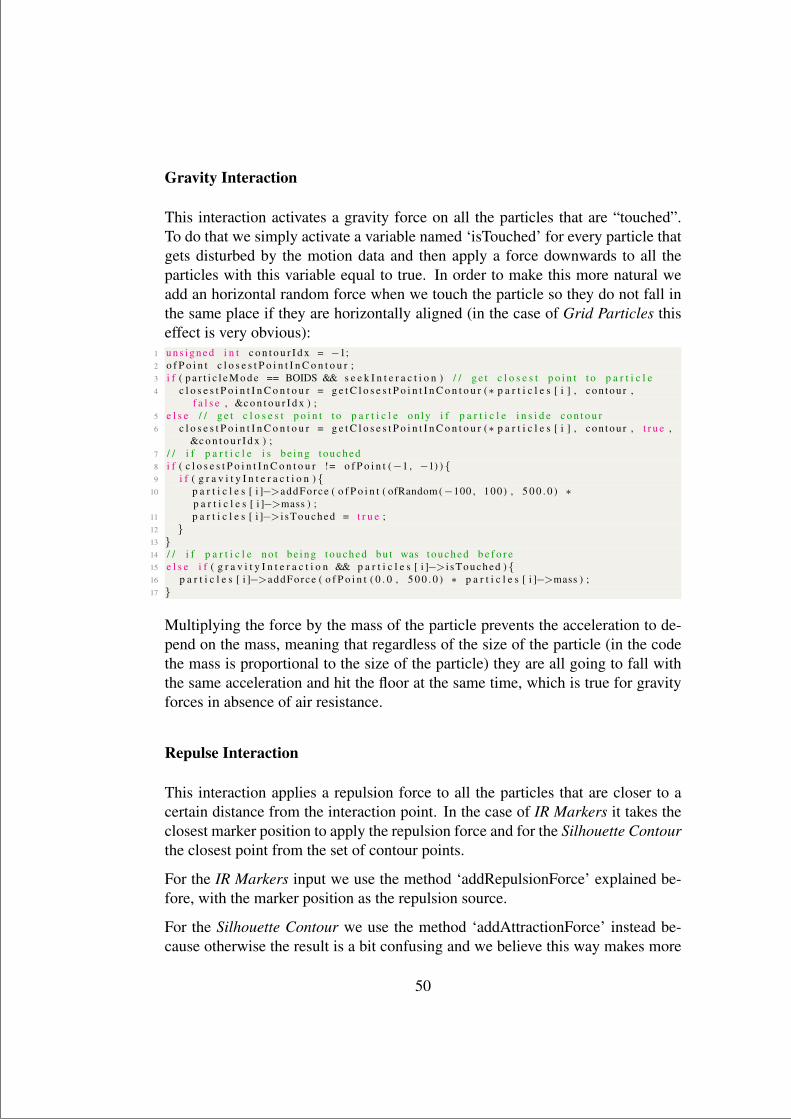
“main” — 2015/7/9 — 12:18 — page 50 — #64

Gravity Interaction

This interaction activates a gravity force on all the particles that are “touched”.To do that we simply activate a variable named ‘isTouched’ for every particle thatgets disturbed by the motion data and then apply a force downwards to all theparticles with this variable equal to true. In order to make this more natural weadd an horizontal random force when we touch the particle so they do not fall inthe same place if they are horizontally aligned (in the case of Grid Particles thiseffect is very obvious):

1 u n s i g n e d i n t c o n t o u r I d x = −1;2 o f P o i n t c l o s e s t P o i n t I n C o n t o u r ;3 i f ( p a r t i c l e M o d e == BOIDS && s e e k I n t e r a c t i o n ) / / g e t c l o s e s t p o i n t t o p a r t i c l e4 c l o s e s t P o i n t I n C o n t o u r = g e t C l o s e s t P o i n t I n C o n t o u r (∗ p a r t i c l e s [ i ] , c o n t o u r ,

f a l s e , &c o n t o u r I d x ) ;5 e l s e / / g e t c l o s e s t p o i n t t o p a r t i c l e on ly i f p a r t i c l e i n s i d e c o n t o u r6 c l o s e s t P o i n t I n C o n t o u r = g e t C l o s e s t P o i n t I n C o n t o u r (∗ p a r t i c l e s [ i ] , c o n t o u r , t r u e ,

&c o n t o u r I d x ) ;7 / / i f p a r t i c l e i s b e i n g t o u c h e d8 i f ( c l o s e s t P o i n t I n C o n t o u r != o f P o i n t (−1 , −1) ) {9 i f ( g r a v i t y I n t e r a c t i o n ) {

10 p a r t i c l e s [ i ]−>addForce ( o f P o i n t ( ofRandom (−100 , 100) , 5 0 0 . 0 ) ∗p a r t i c l e s [ i ]−>mass ) ;

11 p a r t i c l e s [ i ]−> i sTouched = t r u e ;12 }13 }14 / / i f p a r t i c l e n o t b e i n g t o u c h e d b u t was t o u c h e d b e f o r e15 e l s e i f ( g r a v i t y I n t e r a c t i o n && p a r t i c l e s [ i ]−> i sTouched ) {16 p a r t i c l e s [ i ]−>addForce ( o f P o i n t ( 0 . 0 , 5 0 0 . 0 ) ∗ p a r t i c l e s [ i ]−>mass ) ;17 }

Multiplying the force by the mass of the particle prevents the acceleration to de-pend on the mass, meaning that regardless of the size of the particle (in the codethe mass is proportional to the size of the particle) they are all going to fall withthe same acceleration and hit the floor at the same time, which is true for gravityforces in absence of air resistance.

Repulse Interaction

This interaction applies a repulsion force to all the particles that are closer to acertain distance from the interaction point. In the case of IR Markers it takes theclosest marker position to apply the repulsion force and for the Silhouette Contourthe closest point from the set of contour points.

For the IR Markers input we use the method ‘addRepulsionForce’ explained be-fore, with the marker position as the repulsion source.

For the Silhouette Contour we use the method ‘addAttractionForce’ instead be-cause otherwise the result is a bit confusing and we believe this way makes more

50

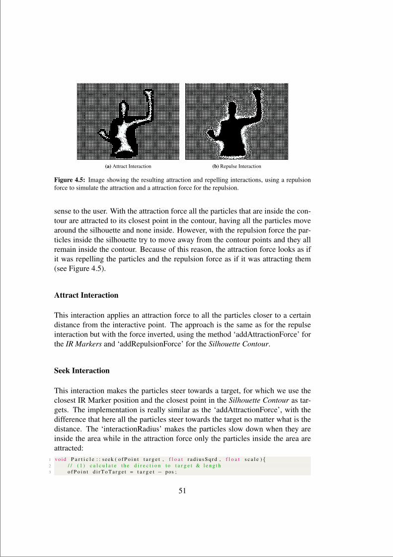
“main” — 2015/7/9 — 12:18 — page 51 — #65

(a) Attract Interaction (b) Repulse Interaction

Figure 4.5: Image showing the resulting attraction and repelling interactions, using a repulsionforce to simulate the attraction and a attraction force for the repulsion.

sense to the user. With the attraction force all the particles that are inside the con-tour are attracted to its closest point in the contour, having all the particles movearound the silhouette and none inside. However, with the repulsion force the par-ticles inside the silhouette try to move away from the contour points and they allremain inside the contour. Because of this reason, the attraction force looks as ifit was repelling the particles and the repulsion force as if it was attracting them(see Figure 4.5).

Attract Interaction

This interaction applies an attraction force to all the particles closer to a certaindistance from the interactive point. The approach is the same as for the repulseinteraction but with the force inverted, using the method ‘addAttractionForce’ forthe IR Markers and ‘addRepulsionForce’ for the Silhouette Contour.

Seek Interaction

This interaction makes the particles steer towards a target, for which we use theclosest IR Marker position and the closest point in the Silhouette Contour as tar-gets. The implementation is really similar as the ‘addAttractionForce’, with thedifference that here all the particles steer towards the target no matter what is thedistance. The ‘interactionRadius’ makes the particles slow down when they areinside the area while in the attraction force only the particles inside the area areattracted:

1 vo id P a r t i c l e : : s eek ( o f P o i n t t a r g e t , f l o a t r a d i u s S q r d , f l o a t s c a l e ) {2 / / ( 1 ) c a l c u l a t e t h e d i r e c t i o n t o t a r g e t & l e n g t h3 o f P o i n t d i r T o T a r g e t = t a r g e t − pos ;

51

“main” — 2015/7/9 — 12:18 — page 52 — #66

4 f l o a t d i s t S q r d = pos . s q u a r e D i s t a n c e ( t a r g e t ) ;5

6 / / ( 2 ) s c a l e f o r c e depend ing on t h e d i s t a n c e7 f l o a t p c t = 1 ;8 i f ( d i s t S q r d < r a d i u s S q r d ) {9 p c t = d i s t S q r d / r a d i u s S q r d ; / / d e c r e a s e f o r c e when c l o s e r t o t a r g e t

10 }11

12 / / ( 3 ) u p d a t e f o r c e13 d i r T o T a r g e t . n o r m a l i z e ( ) ;14 f r c += d i r T o T a r g e t ∗ s c a l e ∗ p c t ;15 }

However, we decided to make all the particles seek the corresponding closestpoints only for the Boids Particles group, for which ‘getClosestPointInContour’and ‘getClosestMarker’ have a special case and return the closest point to theparticle even when this is not inside the silhouette or the interaction area. Thatis the reason why the outcome of this interaction for all the other groups (i.e.,Emitter, Grid, Animations) is similar to the ‘Attraction Interaction’, although theforce in this case is softer and results in a smoother interaction. Below there is thecode used to call this interaction method for both inputs (IR Marker and SilhouetteContour), where you can see the distinction done to get the closest point for theBoids Particles:

1 i f ( m a r k e r s I n p u t ) {2 i r M a r k e r ∗ c l o s e s t M a r k e r ;3 i f ( p a r t i c l e M o d e == BOIDS ) / / g e t c l o s e s t marker t o p a r t i c l e4 c l o s e s t M a r k e r = g e t C l o s e s t M a r k e r (∗ p a r t i c l e s [ i ] , marke r s ) ;5 e l s e / / g e t c l o s e s t marker t o p a r t i c l e on ly i f p a r t i c l e i s i n s i d e i n t e r a c t i o n

a r e a6 c l o s e s t M a r k e r = g e t C l o s e s t M a r k e r (∗ p a r t i c l e s [ i ] , markers ,

i n t e r a c t i o n R a d i u s S q r d ) ;7 i f ( c l o s e s t M a r k e r != NULL) {8 i f ( s e e k I n t e r a c t i o n ) {9 p a r t i c l e s [ i ]−>s eek ( c l o s e s t M a r k e r−>smoothPos , i n t e r a c t i o n R a d i u s S q r d ,

i n t e r a c t i o n F o r c e ∗4 . 0 ) ;10 }11 . . .12 }13 }14 i f ( c o n t o u r I n p u t ) {15 u n s i g n e d i n t c o n t o u r I d x = −1;16 o f P o i n t c l o s e s t P o i n t I n C o n t o u r ;17 i f ( p a r t i c l e M o d e == BOIDS && s e e k I n t e r a c t i o n ) / / g e t c l o s e s t p o i n t t o p a r t i c l e18 c l o s e s t P o i n t I n C o n t o u r = g e t C l o s e s t P o i n t I n C o n t o u r (∗ p a r t i c l e s [ i ] , c o n t o u r ,

f a l s e , &c o n t o u r I d x ) ;19 e l s e / / g e t c l o s e s t p o i n t t o p a r t i c l e on ly i f p a r t i c l e i n s i d e c o n t o u r20 c l o s e s t P o i n t I n C o n t o u r = g e t C l o s e s t P o i n t I n C o n t o u r (∗ p a r t i c l e s [ i ] , c o n t o u r ,

t r u e , &c o n t o u r I d x ) ;21 / / i f p a r t i c l e i s b e i n g t o u c h e d22 i f ( c l o s e s t P o i n t I n C o n t o u r != o f P o i n t (−1 , −1) ) {23 i f ( s e e k I n t e r a c t i o n ) {24 p a r t i c l e s [ i ]−>s eek ( c l o s e s t P o i n t I n C o n t o u r , i n t e r a c t i o n R a d i u s S q r d ,

i n t e r a c t i o n F o r c e ∗4 . 0 ) ;25 }26 . . .27 }

52

“main” — 2015/7/9 — 12:18 — page 53 — #67

28 }

Bounce Interaction

This interaction makes the particles bounce with the surface of the silhouette con-tour, hence it only works when the interaction input is set to Contour (see ap-pendix A). In order to simulate this bounce we created a new method in the parti-cle class that given a set of points conforming a contour it computes the reflectionvector of the particle velocity where it hits this contour and assigns it to the veloc-ity of the particle for the next frame.

The formula to get the reflection of a vector across a plane is the following:

~v′ = ~v − 2(~n · ~v)~n (4.7)

Where ~n is the normal of the plane, ~v the incoming direction vector and ~v′ thereflected vector.

In order to implement this we only need to get the normal vector in the pointwhere the particle hits the contour and apply the previous formula:

1 vo id P a r t i c l e : : con tou rBounce ( o f P o l y l i n e c o n t o u r ) {2 u n s i g n e d i n t i n d e x ;3 o f P o i n t c o n t a c t P o i n t = c o n t o u r . g e t C l o s e s t P o i n t ( pos , &i n d e x ) ;4 ofVec2f normal = c o n t o u r . ge tNormalAt Index ( i n d e x ) ;5 v e l = v e l − 2∗ v e l . d o t ( normal ) ∗normal ; / / r e f l e c t i o n v e c t o r6 v e l ∗= 0 . 3 5 ; / / damping7 }

Whenever an object bounces a surface some of its speed is lost (how much de-pends on the object itself and the surface it hits). That is why we multiply by 0.35the magnitude of the velocity after reflecting it, simulating this loss of speed.

In terms of the particle system, we use the contour index pointer from ‘getClo-sestPointInContour’ method to pass the contour set of points to ‘contourBounce’,which will only be called whenever the particle is inside the silhouette (‘getClo-sestPointInContour’ only returns a point if the given particle is inside the con-tour):

1 u n s i g n e d i n t c o n t o u r I d x = −1;2 o f P o i n t c l o s e s t P o i n t I n C o n t o u r ;3 i f ( p a r t i c l e M o d e == BOIDS && s e e k I n t e r a c t i o n ) / / g e t c l o s e s t p o i n t t o p a r t i c l e4 c l o s e s t P o i n t I n C o n t o u r = g e t C l o s e s t P o i n t I n C o n t o u r (∗ p a r t i c l e s [ i ] , c o n t o u r ,

f a l s e , &c o n t o u r I d x ) ;5 e l s e / / g e t c l o s e s t p o i n t t o p a r t i c l e on ly i f p a r t i c l e i s i n s i d e c o n t o u r6 c l o s e s t P o i n t I n C o n t o u r = g e t C l o s e s t P o i n t I n C o n t o u r (∗ p a r t i c l e s [ i ] , c o n t o u r , t r u e ,

&c o n t o u r I d x ) ;

53

“main” — 2015/7/9 — 12:18 — page 54 — #68

7 i f ( c l o s e s t P o i n t I n C o n t o u r != o f P o i n t (−1 , −1) ) {8 i f ( b o u n c e I n t e r a c t i o n ) {9 i f ( c o n t o u r I d x != −1)

p a r t i c l e s [ i ]−>con tourBounce ( c o n t o u r . c o n t o u r s [ c o n t o u r I d x ] ) ;10 }11 }

4.4.4 Emitter Particles

Creates particles from a source with certain initial attributes (e.g., velocity, radius,color, lifespan). When using the IR Markers as the input source the particlesemitted inherit the velocity of the marker and in Silhouette Contour the velocityfrom the optical flow.

We created three different kinds of emission, both for IR Markers and SilhouetteContour, that differentiate in how the particles are emitted from the two inputsources (see Image 4.6):

Emit all time A constant number of particles is emitted from the inputsource at every frame. In the case of IR Markers in any part within the cir-cular area defined by the marker and for the Silhouette Contour anywhereinside the silhouette.

Emit all time in contour A number of particles are emitted every framebut only on the contour of the input source. In the case of IR Markersaround the circular area defined by the marker and for the Silhouette Con-tour around the silhouette.

Emit only if movement A different number of particles is emitted depend-ing on the velocity of the input source. In the case of IR Markers it maps thevelocity of the marker to emit different amounts of particles, creating moreparticles with higher velocity and no particles if there is no movement. ForSilhouette Contour we use the velocity mask (see section 3.7) to make par-ticles born only on the areas where there has been some movement.

Below there is the code to create ‘n’ particles for the Silhouette Contour inputcase, which is a bit more complex than the IR Markers but the approach is thesame in both. As arguments to the method we pass the amount of particles tocreate, the optical flow data and the set of points conforming the contour areawhere the particles will born (either the contour of the silhouette or the contour ofthe velocity mask so it only emits particles in the motion areas):

1 vo id P a r t i c l e S y s t e m : : a d d P a r t i c l e s ( i n t n , c o n s t o f P o l y l i n e& c o n t o u r , Contour&f low ) {

2 f o r ( i n t i = 0 ; i < n ; i ++){

54

“main” — 2015/7/9 — 12:18 — page 55 — #69

(a) Emit all time (b) Emit all time in contour (c) Emit only if movement

(d) Emit all time (e) Emit all time in contour (f) Emit only if movement

Figure 4.6: Different ways of emitting particles from the two input sources, first row from IRMarkers and second row from Silhouette Contour. Also the silhouette contour is drawn to make iteasier to understand.

3 o f P o i n t pos , randomVel , motionVel , v e l ;4

5 / / C r e a t e random p a r t i c l e s i n s i d e c o n t o u r p o l y l i n e6 i f ( e m i t A l l T i m e I n s i d e | | emitInMovement ) {7 / / u se bounding box t o l i m i t s p a c e o f randomly g e n e r a t e d p o s i t i o n s8 / / and i s f a s t e r t o f i n d a p o s i t i o n which i s i n s i d e c o n t o u r9 o f R e c t a n g l e box = c o n t o u r . getBoundingBox ( ) ;

10 o f P o i n t c e n t e r = box . g e t C e n t e r ( ) ;11 pos . x = c e n t e r . x + ( ofRandom ( 1 . 0 f ) − 0 . 5 f ) ∗ box . ge tWid th ( ) ;12 pos . y = c e n t e r . y + ( ofRandom ( 1 . 0 f ) − 0 . 5 f ) ∗ box . g e t H e i g h t ( ) ;13

14 w h i l e ( ! c o n t o u r . i n s i d e ( pos ) ) {15 pos . x = c e n t e r . x + ( ofRandom ( 1 . 0 f ) − 0 . 5 f ) ∗ box . ge tWid th ( ) ;16 pos . y = c e n t e r . y + ( ofRandom ( 1 . 0 f ) − 0 . 5 f ) ∗ box . g e t H e i g h t ( ) ;17 }18

19 / / s e t v e l o c i t y t o random v e c t o r d i r e c t i o n wi th ’ v e l o c i t y ’ a s magn i tude20 randomVel = randomVector ( ) ∗ ( v e l o c i t y +randomRange ( v e l o c i t y R n d , v e l o c i t y ) ) ;21 }22

23 / / C r e a t e p a r t i c l e s on ly a round t h e c o n t o u r p o l y l i n e24 e l s e i f ( emi tA l lT imeCon tou r ) {25 f l o a t i n d e x I n t e r p o l a t e d = ofRandom ( 0 , c o n t o u r . s i z e ( ) ) ;26 pos = c o n t o u r . g e t P o i n t A t I n d e x I n t e r p o l a t e d ( i n d e x I n t e r p o l a t e d ) ;27

28 / / Use normal v e c t o r i n s u r f a c e as v e l . d i r e c t i o n so p a r t i c l e moves o u t o ft h e c o n t o u r

29 randomVel = −c o n t o u r . g e t N o r m a l A t I n d e x I n t e r p o l a t e d ( i n d e x I n t e r p o l a t e d ) ∗( v e l o c i t y + randomRange ( v e l o c i t y R n d , v e l o c i t y ) ) ;

30 }31

32 / / g e t v e l o c i t y v e c t o r i n p a r t i c l e pos

55

“main” — 2015/7/9 — 12:18 — page 56 — #70

33 mot ionVel = f low . g e t F l o w O f f s e t ( pos ) ∗ ( v e l o c i t y ∗5.0+ randomRange ( v e l o c i t y R n d ,v e l o c i t y ∗5 . 0 ) ) ;

34

35 v e l = randomVel ∗ ( v e l o c i t y R n d / 1 0 0 . 0 ) + mot ionVel ∗ ( v e l o c i t y M o t i o n / 1 0 0 . 0 ) ;36 pos += randomVector ( ) ∗ e m i t t e r S i z e ; / / r andomize p o s i t i o n w i t h i n a r a n g e o f

e m i t t e r s i z e37

38 f l o a t i n i t i a l R a d i u s = r a d i u s + randomRange ( rad iusRnd , r a d i u s ) ;39 f l o a t l i f e t i m e = t h i s−>l i f e t i m e + randomRange ( l i f e t i m e R n d , t h i s−>l i f e t i m e ) ;40

41 a d d P a r t i c l e ( pos , ve l , o f C o l o r ( red , green , b l u e ) , i n i t i a l R a d i u s , l i f e t i m e ) ;42 }43 }

In this code there are a couple of functions that were created that are really usefulto randomize the attributes of the particles and since they are used a lot it is worthmentioning them: (1) randomRange and (2) randomVector.

The first one returns a random unit vector around the unit circle and it is useful toget a random direction. This is the code:

1 o f P o i n t P a r t i c l e S y s t e m : : randomVector ( ) {2 f l o a t a n g l e = ofRandom ( ( f l o a t ) M PI ∗ 2 . 0 f ) ;3 r e t u r n o f P o i n t ( cos ( a n g l e ) , s i n ( a n g l e ) ) ;4 }

The second method, given a scalar value and a percentage of randomness, it re-turns a random value between the range in between the percentage of the valueabove and below. For instance if the percentage is 50 and the value is 4.0, it willreturn a random value between 2.0 and 6.0.

1 f l o a t P a r t i c l e S y s t e m : : randomRange ( f l o a t p e r c e n t a g e , f l o a t v a l u e ) {2 r e t u r n ofRandom ( va lue −( p e r c e n t a g e / 1 0 0 ) ∗ va lue , v a l u e +( p e r c e n t a g e / 1 0 0 ) ∗ v a l u e ) ;3 }

4.4.5 Grid Particles

Grid Particles creates a grid of a fixed number of particles with infinite lifetimefilling the output window. Basically it creates a particle with zero initial velocityevery certain distance when we initialize the particle system. It does so by callingthe following method:

1 vo id P a r t i c l e S y s t e m : : c r e a t e P a r t i c l e G r i d ( i n t width , i n t h e i g h t ) {2 f o r ( i n t y = 0 ; y < h e i g h t / g r i d R e s ; y ++){3 f o r ( i n t x = 0 ; x < wid th / g r i d R e s ; x ++){4 i n t x i = ( x + 0 . 5 f ) ∗ g r i d R e s ;5 i n t y i = ( y + 0 . 5 f ) ∗ g r i d R e s ;6 o f P o i n t v e l = o f P o i n t ( 0 , 0 ) ;7 a d d P a r t i c l e ( o f P o i n t ( xi , y i ) , ve l , o f C o l o r ( red , green , b l u e ) , r a d i u s ,

l i f e t i m e ) ;8 }9 }

10 }

56

“main” — 2015/7/9 — 12:18 — page 57 — #71

One special feature of this particle system is the use of the stored initial positionof the particle to make the particle return to its initial state after applying an inte-raction force. This creates a very natural effect and makes the grid remain intacteven after applying different forces to the particles. The method that does thisis very similar to the one explained in ‘Seek Interaction’ but it uses the initialposition as a fixed target:

1 vo id P a r t i c l e : : r e t u r n T o O r i g i n ( f l o a t r a d i u s S q r d , f l o a t s c a l e ) {2 / / ( 1 ) c a l c u l a t e t h e d i r e c t i o n t o o r i g i n p o s i t i o n and d i s t a n c e3 o f P o i n t d i r T o O r i g i n = i n i P o s − pos ;4 f l o a t d i s t S q r d = pos . s q u a r e D i s t a n c e ( i n i P o s ) ;5

6 / / ( 2 ) s e t f o r c e depend ing on t h e d i s t a n c e7 f l o a t p c t = 1 ;8 i f ( d i s t S q r d < r a d i u s S q r d ) {9 p c t = d i s t S q r d / r a d i u s S q r d ; / / d e c r e a s e f o r c e when c l o s e r t o o r i g i n

10 }11

12 / / ( 3 ) u p d a t e f o r c e13 d i r T o O r i g i n . n o r m a l i z e ( ) ;14 f r c += d i r T o O r i g i n ∗ s c a l e ∗ p c t ;15 }

4.4.6 Boids Particles

Creates a fixed number of particles with infinite lifetime that simulate a flockingbehavior.

[Reynolds, 1987] is the first article describing a computer model, that the authornamed Boids, to emulate the flocking behavior; boid is each of the free agentsthat form the flock which in our implementation is the same as a particle. Thebasic model consists of three simple rules that describe how each individual boidbehaves based on the positions and velocities of the boids nearby: (1) Separation,(2) Alignment and (3) Cohesion. However, we can add more rules to extend themodel in several different ways, like make the flocks avoid obstacles or seek aspecific target.

There are many source codes to implement this algorithm but our code is based ona Cinder tutorial9. Chapter 6: Autonomous Agents in [Shiffman, 2012] describesthe model step by step and it is a great source to understand the basics and getsome ideas on how to extend its functionality.

The three basic rules of the flocking algorithm (see Figure 4.7) that are applied toeach of the boids of the system are the following:

9http://libcinder.org/docs/dev/flocking chapter1.html

57

“main” — 2015/7/9 — 12:18 — page 58 — #72

Separation The separation rule makes the particle move away from itsneighbors, avoiding collisions between them. To do that it checks all theboids within the flocking radius (distance at which the other boids are con-sidered flockmates) to see if the distance between them is too small, and ifso, adds a repulsion force to move away from them.

Cohesion The cohesion or attraction rule makes the particle stay close to-gether with their flockmates, moving towards the center of its neighbors. Inorder to do that it averages the location of all the boids within the flockingradius and moves towards this average location.

Alignment The alignment rule makes the particle move in the same direc-tion as its neighbors if it is not too far nor too close from them. In orderto do that it averages the velocity vectors of all the boids within the flock-ing radius (average direction of the flock) and it steers to move in the samedirection.

By combining these three rules we simulate the flocking behavior, using the sametechnique as in ‘Particle-particle repulsion’ to speed up the comparisons betweenthe different particles. We compare each pair of particles only once and break thesecond loop when the distance between particles is too far:

1 vo id P a r t i c l e S y s t e m : : f l o c k P a r t i c l e s ( ) {2 f o r ( i n t i = 0 ; i < p a r t i c l e s . s i z e ( ) ; i ++){3 f o r ( i n t j = i −1; j >= 0 ; j−−){4 i f ( f a b s ( p a r t i c l e s [ i ]−>pos . x − p a r t i c l e s [ j ]−>pos . x ) > f l o c k i n g R a d i u s )

b r e a k ;5 p a r t i c l e s [ i ]−>a d d F l o c k i n g F o r c e s (∗ p a r t i c l e s [ j ] ) ;6 }7 }8 }

And the code inside the particle class to apply the flocking forces is the follow-ing:

1 vo id P a r t i c l e : : a d d F l o c k i n g F o r c e s ( P a r t i c l e &p ) {2 o f P o i n t d i r = pos − p . pos ;3 f l o a t d i s t S q r d = pos . s q u a r e D i s t a n c e ( p . pos ) ;4

5 i f ( 0 . 0 1 f < d i s t S q r d && d i s t S q r d < f l o c k i n g R a d i u s S q r d ) { / / i f n e i g h b o r p a r t i c l ew i t h i n zone r a d i u s . . .

6 f l o a t p e r c e n t = d i s t S q r d / f l o c k i n g R a d i u s S q r d ;7

8 / / S e p a r a t e9 i f ( p e r c e n t < lowThresh ) { / / . . . and i s w i t h i n t h e lower t h r e s h o l d

l i m i t s , s e p a r a t e10 f l o a t F = ( lowThresh / p e r c e n t − 1 . 0 f ) ∗ s e p a r a t i o n S t r e n g t h ;11 d i r = d i r . g e t N o r m a l i z e d ( ) ∗ F ;12 f r c += d i r ;13 p . f r c −= d i r ;14 }15 / / A l ign

58

“main” — 2015/7/9 — 12:18 — page 59 — #73

(a) Separation (b) Cohesion (c) Alignment

Figure 4.7: Flocking behavior basic rules10.

16 e l s e i f ( p e r c e n t < h i g h T h r e s h ) { / / . . . e l s e i f i t i s w i t h i n t h e h i g h e rt h r e s h o l d l i m i t s , a l i g n

17 f l o a t t h r e s h D e l t a = h i g h T h r e s h − lowThresh ;18 f l o a t a d j u s t e d P e r c e n t = ( p e r c e n t − lowThresh ) / t h r e s h D e l t a ;19 f l o a t F = ( 0 . 5 f − cos ( a d j u s t e d P e r c e n t ∗ M PI ∗ 2 . 0 f ) ∗ 0 . 5 f + 0 . 5 f ) ∗

a l i g n m e n t S t r e n g t h ;20 f r c += p . v e l . g e t N o r m a l i z e d ( ) ∗ F ;21 p . f r c += v e l . g e t N o r m a l i z e d ( ) ∗ F ;22 }23 / / A t t r a c t24 e l s e { / / . . . e l s e , a t t r a c t25 f l o a t t h r e s h D e l t a = 1 . 0 f − h i g h T h r e s h ;26 f l o a t a d j u s t e d P e r c e n t = ( p e r c e n t − h i g h T h r e s h ) / t h r e s h D e l t a ;27 f l o a t F = ( 0 . 5 f − cos ( a d j u s t e d P e r c e n t ∗ M PI ∗ 2 . 0 f ) ∗ 0 . 5 f + 0 . 5 f ) ∗

a t t r a c t i o n S t r e n g t h ;28 d i r = d i r . g e t N o r m a l i z e d ( ) ∗ F ;29 f r c −= d i r ;30 p . f r c += d i r ;31 }32 }33 }

If the particle we are comparing with is within the flocking radius we add it asa neighbor and we compute the flocking forces that apply to both particles. De-pending on how far are the particles we apply one or another rule. If the particlesare too close we apply a separation force, if they are too far an attraction force andotherwise we just align their velocities. The values used to compute the force ‘F’that we can see in the previous code are just to make the transitions between onerule to the other smoother and more natural.

4.4.7 Animations Particles

Creates particles with different lifetimes simulating three predefined effect anima-tions:

10http://www.red3d.com/cwr/boids/

59

“main” — 2015/7/9 — 12:18 — page 60 — #74

Rain Simulates rain by creating small particles on the upper part of theoutput window with an initial velocity and a gravity force downwards.

Snow Simulates snow by creating medium-sized particles on the upper partof the output window with an initial velocity and gravity downwards andsome Perlin noise to simulate the randomness of the snow flakes fallingdown.

Explosion Simulates an explosion by creating various particles at once onthe bottom part of the output window with a big initial velocity upwards. Italso has some gravity force downwards and high friction that simulates theparticles slowing down by its own weight. Finally we add some noise usingthe method ‘addNoise’ described in section 4.4.2 to give a more organiclook.

4.4.8 Fluid particles

Creates particles based on the fluid flow from the fluid solver, which can eitherbe interacted by the IR Markers or the Silhouette Contour. This is a feature thatcomes with the ofxFlowTools addon and it uses the OpenGL Shading Languageto create and update the particles behavior; it takes advantage of the parallelismfrom the GPU to create a great number of particles without slowing down thesystem.

Particles change their acceleration based on the fluid velocity and the optical flowtextures at each time step, using a very similar approach to the one described insection 4.4.1 to update the motion of the particles. However, here it makes use oftextures to take advantage of the GPU instead of doing all the computations in theCPU as in the previous particle system groups.

The implementation consists of a pair of four-channel textures of size (i.e.,width×height) equal to the maximum number of particles that we will want to draw inone frame, saving in each pixel the state of a single particle. The first texture savesfour basic attributes: age, lifespan, mass and size. The second texture includes theposition of the particle, ‘x’ and ‘y’ coordinate, using only the first two channelsof the texture (see Figure 4.8). In fact, these textures are duplicated due to the factthat a texture cannot be used as input and output at the same time. Because of thatwe have to use a pair of textures and a double buffering technique (often namedPing-pong technique11) to be able to compute the new data from the previous val-ues; we save the current data to one texture while we read from the other and then

11http://www.pixelnerve.com/v/2010/07/20/pingpong-technique/

60

“main” — 2015/7/9 — 12:18 — page 61 — #75

we swap their roles.

Figure 4.8: Diagram showing the two textures containing the state attributes of the particles wetransfer to the GPU to update its behavior over time. In this example we could only draw 16particles (16 pixels in the texture, although 4 particles are dead) and the red square represents thered particle in the screen (the numbers in the matrices are not exact and it is only to help understandthe implementation).

With the use of fragment shaders we update each pixel (i.e., particle attributes) ofthe textures at every frame; the fluid velocity and optical flow textures are usedto update the particle position and to create new particles and the elapsed timesince the application started is used to update their age. As a last step it takesthe information stored in these pair of textures to draw the particles in the screen;given a mesh of vertices (with as many vertices as particles) it uses a vertex shaderto draw each vertex as a circle, of size equal to the particle radius attribute, in thecorresponding position.

Very briefly explained, a fragment shader assigns a color value to each pixel anda vertex shader takes a vertex array and transforms these vertices through a seriesof operations to show them in the screen space.

The way it decides how many particles to create at every iteration is based ona couple of variables: (1) particlesBirthChance and (2) particlesBirthVelocity-Chance, and the amount of motion in each pixel of the screen. These are thesteps:

1. The fragment shader checks for every dead particle (pixel with age attributeequal to 0), if there is velocity data in that position. If so, it computes arandom value.

2. This random value is compared with ‘particlesBirthChance’ and if it is

61

“main” — 2015/7/9 — 12:18 — page 62 — #76

lower, it creates a new particle in this pixel position.

3. This particle is initialized with the attributes previously defined for the par-ticle system (lifespan, mass and size) and it starts counting its age at everyframe.

Having said that, we can see that the larger the value of ‘particlesBirthChance’the most likely will be that new particles are created. On the other hand, therandom computed value in 1 is divided by ‘particlesBirthVelocityChance’ beforecomparing it with ‘particlesBirthChance’ in 2, meaning that if the value is high,the random value will be smaller and hence will be also more likely that this islower than the threshold to create a new particle. Moreover, the value of ‘par-ticlesBirthVelocityChance’ is directly proportional to the velocity in that pixel,meaning that if the velocity is high it will be more likely that new particles arecreated.

4.5 Silhouette Representation

Figure 4.9: Polygon withvertex G non-convex. A ver-tex is called convex if the an-gle formed by its two edges,with the polygon inside theangle, is less than 180◦.

These are the graphics that represent the silhouette ofthe dancer in a few different ways (see Figure 4.10). Atfirst the idea was to create some more options but weended up deciding to focus on other parts of the systemand just create a few examples. The output possibili-ties are (1) silhouette, (2) convex hull and (3) boundingrectangle. These were inspired by the performance Di-sorder12 by CENC (Centre d’Expression Numerique etCorporelle).

Silhouette takes the set of points from the silhouettecontour and considers them as vertices of a closedpolygon. Applying a weighted arithmetic mean be-tween the vertices we make the silhouette look lessnoisy and smoother, being able to set the amount ofsmoothness by taking more or less vertices in comput-ing the average. If the smoothing size is two, for everyvertex in the polygon we take the two vertices on itsleft, the two on its right and the current vertex and apply a weighted average withall of them, giving more priority (more weight) to the closer vertices to the cur-rent.

12https://vimeo.com/32111537

62

“main” — 2015/7/9 — 12:18 — page 63 — #77

Convex hull is the smallest convex region enclosing the set of contour points,using the algorithm described in [Sklansky, 1982]. The idea of this algorithm isquite simple. Assuming we have the set of vertices of the polygon ordered, westart the algorithm from one of its four extremal vertices (leftmost, rightmost, topor bottom). At each step we look at the two consecutive vertices (left and right)and compute an equation to determine whether the middle vertex is convex or not(see Figure 4.9). If the vertex is not convex this is deleted and we regress onevertex to check if the vertex is still convex. The algorithm ends when we checkthe vertex we started the algorithm with.

The steps we just described only work for certain simple polygons and the algo-rithm OpenCV uses does a few more operations but the principle is the same.

Bounding rectangle is the smallest rectangle enclosing the set of contour pointssubject to the constraint that the edges of the rectangle are parallel to the coor-dinate axes (window margins). The resulting bounding rectangle is the same asthe minimum rectangle enclosing the convex hull, which is faster to compute.The rectangle is defined by the minimal and maximal value of the correspondingcoordinate (x, y) for the set of points of the polygon:

{(min(x),min(y)

),(max(x),min(y)

),(min(x),max(y)

),(max(x),max(y)

)}

(a) Silhouette (b) Convex Hull (c) Bounding Rectangle

(d) Silhouette Line (e) Convex Hull Line (f) Bounding Rectangle Line

Figure 4.10: Silhouette representation graphic possibilities.

63

“main” — 2015/7/9 — 12:18 — page 64 — #78

4.6 Conclusions

In this chapter we covered the algorithms that have been used in the CREA sys-tem.

The results obtained after implementing the graphic algorithms are satisfactory.The graphics respond very naturally to the motion capture data and after havingadapted some of the algorithms to make them more effective, the system workssmoothly in real-time even when generating the most computationally expensivegraphics. Having said that, we consider the requirements specified for this parthave been fulfilled satisfactorily.

However, if I had to start this part of the project again I would probably changea few things. My idea from the start was to create a tool with as many graphicalvariety choices as possible within the area of particle systems, abstract silhouetterepresentation and fluid simulation. Now I would focus on fewer graphical possi-bilities in order to have more time to explore deeply all of them. For each of theparticle system types created there is a whole world to explore, as well as for thefluids simulation and silhouette representation; slightly changing a few attributesgives a complete new way of interactional behavior.

One thing I wanted to explore more but I haven’t had time enough is the use of theGPU to create more complex particle systems. This is a thing for which you firstneed to understand good enough how particle systems work and the algorithmsinvolved in creating the specific behavior we want to simulate. By using the CPUwe can prototype the particle system behavior with a few hundred particles andthen port it to the GPU. When I started this project I didn’t have experience insimulating particle systems behaviors nor with the workflow to use the GPU func-tionalities but now I consider I have the knowledge enough to explore these.

Furthermore, I also wanted to explore the techniques that optimize the compar-isons between particles in the CPU by spatially organizing them in data structures,such as geometric hashing13 and quad-trees14,15.

The graphics component is closely tied to the rest of the CREA application so inthe final chapter I include the overall conclusions.

13http://en.wikipedia.org/wiki/Geometric hashing14http://en.wikipedia.org/wiki/Quadtree15http://forum.openframeworks.cc/t/quadtree-particle-system

64

“main” — 2015/7/9 — 12:18 — page 65 — #79

Chapter 5

CREA: SYSTEM PROTOTYPE

The two previous chapters have explained the motion capture and the graphicsgeneration parts of the system. This chapter includes the requirements used todevelop the overall system, then it goes over the system architecture, the imple-mentation of all the other relevant components not yet explained in the previouschapters and it finishes with a short conclusion.

5.1 Introduction

The motion capture and generation graphics algorithms used in CREA have beenalready discussed in the previous chapters but there were many other things thathad to be done to develop the overall system and to make it a useful tool in a liveperformance setting.

Figure 5.1 summarizes the functional blocks of the overall system. Apart fromthe motion capture and graphics generation, we created a graphical user interfaceto configure the parameters to be used in a particular performance and to controlthe behavior of the system during the actual performance. In order to set up theset of graphics that will be used in the performance we created the Cue List mo-dule. This allows the user of the system to save a sequence of graphic settingsand switch between them with a smooth transition. The system also integratespreliminary research results on gesture following developed by Cheng-i Wang andShlomo Dubnov ([Wang and Dubnov, 2014]). This tool allows us to recognizepatterns from a prerecorded sequence and use the output to change the graphicsettings automatically.

65

“main” — 2015/7/9 — 12:18 — page 66 — #80

The project has been developed under the openFrameworks toolkit1. Its addonsand its community have been an essential part to fulfill the requirements of thisproject. Also thanks to other open source projects I have been able to learnbest programming practices and use existing code to be able to make the toolmore interesting. Because of that I decided to use an open source license for myproject.

In order to manage the software development process of the project and havecontrol over the different versions of the software I used the GitHub platform.This platform allowed me to share the code with other people and at the same timework collaboratively to implement the Gesture Follower feature (see section 5.6).Moreover, since I wanted CREA to be an open source project, GitHub allowed meto publicly publish the code under an open source license. I chose to license thecode under the GNU Affero License Version 3, which is a copyleft license2.

Dancer + IR Markers

Motion Capture

Cue List

Gesture Follower

Graphics Generation

ControlInterface

Video Image

Settings File(XML)

Cue File(XML)

Gesture Sequence

(XML)

Assistant

Figure 5.1: Block diagram of the CREA system

5.2 Requirements

The requirements of the overall system are a consequence of the user scenario thatwe defined and were elaborated at the beginning of the project while talking withpossible users and my advisors. The specific requirements for the motion capturemodule and the graphics generation have been already explained in the previouschapters. Below we list the general requirements that we defined. First we men-

1http://openframeworks.cc/2http://www.gnu.org/licenses/agpl-3.0.en.html

66

“main” — 2015/7/9 — 12:18 — page 67 — #81

tion the functional requirements and then we continue with the non-functionalones.

5.2.1 Functional Requirements

The system must fulfill the following functional requirements:

1. Motion CaptureCREA must have a motion capture module from which get the motion datafrom the users movement using the Microsoft Kinect depth sensor.

2. Graphics GenerationCREA must have a graphics generation module that creates different graph-ics based on the motion data.

3. Control InterfaceCREA must have a control interface to have control over the motion captureand graphics generation modules. This control interface must allow to con-figure the parameters to be used in a particular performance and to controlthe behavior of the system during the actual performance.

4. Gesture FollowerCREA must have the elements necessary to integrate a gesture followingalgorithm developed by Cheng-i Wang and Shlomo Dubnov.

5.2.2 Non-functional Requirements

The non-functional requirements that the graphics system should fulfill:

1. Open sourceCREA source code shall be publicly available online under an open sourcelicense.

2. Real-timeCREA shall be computationally efficient and fast so it can run in real-time.

3. Platform compatibilityCREA shall work in Windows, Linux and OS X systems.

4. ImplementationCREA has to be written under the openFrameworks toolkit using the C++programming language.

67

“main” — 2015/7/9 — 12:18 — page 68 — #82

5. ExtensibilityCREA shall be easy to extend in order to add new functionalities. In order todo that it should also include documentation so other users can understandand use all the current features.

6. User friendlyCREA shall be easy to learn even to novice technology users.

7. UsabilityCREA shall allow a choreographer to prepare a dance performance offlineand have control over the system during the live performance.

8. Crash recoveryCREA shall be capable to restart fast in case of unexpected crashes anderrors.

9. PortabilityCREA shall be able to adapt to different physical environments, with differ-ent lighting conditions and setups.

10. PriceThe hardware and system on top of which CREA is used shall be affordable.

5.3 Overall System Architecture

Having the list of functionalities that we wanted the system to have we conductedan object-oriented design of the software to decide the different objects and com-ponents required to meet all the requirements. Figure 5.4 shows the result of thisprocess at a high-level of abstraction without much details. The figure shows howthe different classes/objects interrelate and interact.

We describe below the main classes that conform CREA:

ofApp Contains instances to all the other classes and manages their behav-ior by means of the control interface.

irMarker Defines the IR Markers objects that we track from the infrareddata stream, containing the position and velocity information.

Contour Contains all the functionalities that come from the depth mapstream. This includes the computation of the optical flow (see section 3.6),the motion contours using velocity mask (see see section 3.7) and the dif-ferent ways of representing the silhouette contour (see section 4.5).

68

“main” — 2015/7/9 — 12:18 — page 69 — #83

Fluid Describes all the functionalities related to the fluid solver and fluidsimulation (see 4.3). Solves the equations of fluid dynamics to simulate atwo-dimensional fluid behavior and contains the methods to use the state ofthe fluid to interact with other objects.

ParticleSystem Describes a particle system. Contains a dynamic numberof particles and defines the set of rules they have to follow to simulate vari-ous behaviors.

Particle Describes a single particle. Contains the basic functionality tomake this particle move around the screen and update its motion by meansof applying external forces.

Sequence Describes the sequence of the positions of the IR Markers in aperiod of time (gesture).

vmo Contains the functionality to follow gestures from a previously recordedsequence of IR Markers positions.

Following the structure of every openFrameworks project, there is always threebasic files (main.cpp, ofApp.cpp and ofApp.h) that contain the core structure torun the project and create a window for visual output. In the ‘ofApp’ class thereis a ‘setup’, ‘update’ and ‘draw’ methods. Very briefly explained, ‘setup’ is wherewe initialize all the variables and parameters of the application, since it is calledjust once at the start of the project. Right after ‘setup’ there is ‘update’, whichis where we perform all the computations to update the state of our applicationin an infinite cycle that is called at every frame until we finish the application.Finally there is ‘draw’, which is called right after ‘update’ and it performs all thedrawing functions to visualize the application in the screen. Because of this, itis in this class where we have instances to all the other classes and manage theproject behavior by means of the control interface.

5.4 Control Interface

The control interface had to be easy to understand and user-friendly, with a ba-lance between simplicity and usability; a novice user would have to be able to usethe basic features but at the same time a curious and experienced user should havethe options enough to customize better the graphics and control more advancedsettings.

After looking over all the different GUI addons created for openFrameworks we

69

“main” — 2015/7/9 — 12:18 — page 70 — #84

decided to use ofxUI3. This addon is easy to use, very fast, with minimalist de-sign, beautiful aesthetics and very presentable to novice technology users. More-over, this includes a saving/loading functionality of the widget values, which werequired in order to be able to save and load the settings of the control inter-face.

Having decided all the requirements of the system we designed the control inter-face in a way that all the functionalities would be separated in different panels,each with a very clear purpose. We identified 14 different elements for which wewould require independent interface controls:

Basics General functions of the control interface and CREA (i.e., save/loadcontrol interface settings, change output window background color, numberof frames to transition between graphic scenes...)

Kinect All parameters that control how we process the data of the Kinectinput streams. These should allow us to calibrate the Kinect to a particularphysical space (see section 3.3).

Gesture Follower Settings to control the gesture follower (i.e., record se-quence of IR Markers, start/stop gesture tracking, mapping of the recog-nized gestures to graphic outputs... see section 5.6).

Cue List Sequence of graphic settings that allows us to switch from one tothe other in a smooth transition (see section 5.5).

Optical Flow Settings to control the optical flow output (i.e., strength of theoutput velocities, blur velocities over time, threshold to consider motion...see section 3.6).

Velocity Mask Settings to control the velocity mask output (see section3.7).

Fluid Solver Settings to control the fluid properties (i.e., viscosity, vortic-ity, dissipation... see section 4.3).

Fluid Simulation Settings to control the color of the fluid simulation andhow we inject new values to the fluid solver (see section 4.3.2).

Fluid Particles Properties of the particles based on the fluid flow from thefluid solver (mass, size, number of particles... see section 4.4.8).

Silhouette Contour Different ways of representing the silhouette contourplus a few settings to modify this representation (see section 4.5).

3https://github.com/rezaali/ofxUI

70

“main” — 2015/7/9 — 12:18 — page 71 — #85

Emitter Particles Settings to control Emitter Particles behavior (see sec-tion 4.4.4).

Grid Particles Settings to control Grid Particles behavior (see section 4.4.5).

Boids Particles Settings to control Boids Particles behavior (see section4.4.6).

Animations Particles Settings to control Animations Particles behavior (seesection 4.4.7).

Having all these elements, we defined the most relevant controls for each of them,thinking on which values made more sense to be able to manipulate. Next wehad to define which type of GUI widgets use for each of the controls (i.e., toggle,button, slider, text box...) and plan how they would react to the system. The nextstep was to structure all the controls around the window in a way that was as clearand simple as possible, adding all the elements that we thought were useful tounderstand the current status of the system. At the end we decided to group the14 panels we have mentioned in 8 different menus (see Appendix A).

In order to save/load the settings of the control interface we defined our own for-mat using XML, taking advantage of the XML functionalities that come with theofxUI addon. In this way we were able to decide which widget values we wantedto save in the file and which not. Furthermore, we defined two different waysof loading the settings files: (1) change all the current values to the ones in thefile immediately or (2) gradually interpolate between the current values and theones in the file within a determined number of frames (see ‘saveGUISettings’ and‘loadGUISettings’ methods inside ofApp.cpp file for more details).

Implementing (2) was a bit more complicated. The approach we use is to savethe original value and the goal value for each of the widgets and use the numberof frames elapsed since we loaded the settings file to compute the current value.In order to do that we created a map container with a pointer to each widget askey and a vector of floats as the mapped value for each key. Then we just storethe initial value in the first position of the vector and the goal value to the second,interpolating these two values at every frame in order to get the current value (see‘interpolateWidgetValues’ method inside ofApp.cpp file for more details).

5.5 Cue List

Cue List is a simple feature we created to save different graphic settings (cues) ina list and be able to switch from one to the next in a smooth transition (see Figure

71

“main” — 2015/7/9 — 12:18 — page 72 — #86

5.2). This includes some basic functionalities to manage the list, such as creatingnew cues, delete them, put a name to the cue and save/load cues as XML files. Inthis way we can design the sequence of graphics we want to have for a particularperformance.

Figure 5.2: Cue List panel in the controlinterface.

The save/load approach is very similar tothe one used for the control interface set-tings (in fact we use the same methods);the only difference is that for the cues weonly save and load the settings values be-longing to the graphics.

We created a trigger button (‘GO’) thatwhen is pressed loads the next cue inthe list by interpolating the settings val-ues, as explained before. Moreover, wecreated some methods inside each of theclasses containing output graphics (Parti-cleSystem, Contour and Fluid) to do a fadein/out of the drawing opacity when they getactivated/deactivated.

5.6 Gesture Follower

As said in Chapter 1, one of the the goals of the project was to combine CREAwith a prototype of a gesture tracking technology implemented by Cheng-i Wangand Shlomo Dubnov. The idea of this tool is to give the performer the freedomto improvise from a set of recorded gestures and have the system dynamicallychange based on his movements.

[Wang and Dubnov, 2014] introduced a data structure (VMO) capable of identify-ing repetitive fragments and finding sequential similarities between observations.In [Dubnov et al., 2014] they used these properties for tracking and recognizinggestures in real-time, using the positions of the IR Markers as a representation of agesture (sequence). First they record a long sequence with the intended gestures tobe recognized and then using the ‘VMO’ they are able to recognize sub-portions(gestures) of the piece. In [Wang and Dubnov, 2015] this gesture tracking was im-proved by automatically capturing repeated sub-segments from the long sequencewith no manual interaction.

This technology had to be implemented using C++ within the openFrameworks

72

“main” — 2015/7/9 — 12:18 — page 73 — #87

environment in order to be used from CREA. Moreover, in CREA we had to im-plement several features to be able to use the gesture follower. We explain verybriefly some of these features.

One of the most important things to do was save the gestures done with the mar-kers (sequence of its position over time) in a way that could be used to feed thegesture follower. We created our file format for saving this sequence of positionsin an XML file. Since there can be more than one marker in one same frame andwe can loose track of them, we had to take that into consideration when writingthe marker information over time. Besides this, we had to implement the methodthat could read these files in a robust way and store the data in memory so thegesture follower could later use it.

(a) Cue Mapping

(b) Cue with Emitter particles (c) Cue with Grid particles

Figure 5.3: Snapshots of using the Gesture Follower in CREA. The colored line represents thestored sequence, with each color belonging to different graphics (cues). Since we have four cuesin the Cue List we can see four different colors.

Besides this, we had to implement several functionalities to show the output of thetracking in real-time and devise a way to map this output to the graphics duringa performance. In Figure 5.3 the colored line represents the stored gesture (se-quence of 2D points from one IR Marker) with different colors indicating map-pings to different graphics (cues). The bigger circle is the input marker and the

73

“main” — 2015/7/9 — 12:18 — page 74 — #88

green small circle along the trajectory is the current gesture-following position onthe stored gesture corresponding to the input marker. As we can see, the systemgenerates different graphics when the gesture following position (green circle)traverses onto different segments of the stored gesture represented by differentcolors. These segments can be defined through the control interface by sayingwhich percentage from the long sequence assign to each of the cues in the CueList (see Figure 5.3a).

5.7 Conclusions

In this chapter we have presented all the components of CREA that were not yetexplained in the previous chapters. The Gesture Follower feature is still under aresearch phase and that is why we didn’t enter in much detail. In terms of the useof the control interface you can find more details in the appendix A.

74

“main” — 2015/7/9 — 12:18 — page 75 — #89

ParticleSystem

+particles: vector<Particle>+markersInput: bool+contourInput: bool+particleMode: int+gravity: vec2f

+addParticles(int n)+killParticles(int n)+createParticleGrid()

Particle

+id: float {id}+pos: vec2f+vel: vec2f+acc: vec2f+frc: vec2f+friction: float

+addForce(vec2f force)+addNoise(float turbulence)+addAttractionForce(vec2f p)+addRepulsionForce(vec2f p)

ofApp

+irImage: image+depthImage: image+irMarkers: vector<irMarker>+contour: Contour+fluid: Fluid+gui: User Interface+emitterParticles: ParticleSystem+gridParticles: ParticleSystem+boidsParticles: ParticleSystem+animationsParticles: ParticleSystem+sequence: Sequence+vmo: vmo

+saveGUISettings(string path, bool isCue)+loadGUISettings(string path, bool isCue, bool interpolate)

Contour

+silhouette: polyline+convexHull: polyline+boundingRect: polyline+velocityMask: texture+opticalFlow: texture

+getFlowOffset(vec2f p)

Fluid

+fluidFlow: texture+markersInput: bool+contourInput: bool+fluidParticles: texture

+getFluidOffset(vec2f p)

irMarker

+currentPos: vec2f+previousPos: vec2f+smoothPos: vec2f+velocity: vec2f+hasDisappeared: bool

Sequence

+markersSequence: vector<polyline>+patterns: vector<vector<polyline>>

+save(string path)+load(string path)+record(vector<irMarker> irMarkers)

vmo

+currentIdx: int+pttrList: vector+obs: vector

Crea::Main

Figure 5.4: CREA UML Class Diagram with the basic class functionalities.

75

“main” — 2015/7/9 — 12:18 — page 76 — #90

“main” — 2015/7/9 — 12:18 — page 77 — #91

Chapter 6

EVALUATION AND TESTING

This chapter explains how CREA, the system developed as part of this project,was tested on a real context and reports on the feedback obtained from these test-ings.

6.1 Introduction

As it has been explained before, CREA is an application designed to be used in anartistic context. Therefore, CREA had to be tested emulating a real performancewith people experienced in the field in order to evaluate wether it met all therequirements defined in section 5.2.

The development of CREA has been done through a sequence of constant anditerative evaluations. As soon as we had a working prototype, we tested its func-tionalities emulating as close as possible a real performance context. Thanks to adancer close to the project we were able to emulate better real case scenarios andadapt the system to be useful within that context.

Throughout the last two months of the development of CREA this has been testeda total of four times in a performance context, not only with the mentioned dancerbut also with other dancers and regular users. We have set up the system in threedifferent spaces and this has been really helpful in evaluating the portability of thesystem.

In terms of hardware, CREA has been tested on several computers running diffe-rent operating systems. This is the list of the different system configurations whereit has been tested on:

77

“main” — 2015/7/9 — 12:18 — page 78 — #92

1. MacBook Pro (2015) with Intel Core i5 2.7 GHz processor and Intel IrisGraphics 6100 graphic card, with 8 GB RAM. Running OS X Yosemite.

2. MacBook Pro (2013) with Intel Core i5 2.4 GHz processor and Intel Iris5100 graphic card, with 4 GB RAM. Running OS X Yosemite.

3. MacBook Pro (2012) with Intel Core i5 1.8 GHz processor and HD Graph-ics 4000 graphic card, with 4 GB RAM. Running OS X Mavericks.

4. MacBook (2009) with Intel Core 2 Duo 2.26 GHz processor and NVIDIAGeForce 9400M graphic card, with 4 GB RAM. Running OS X MountainLion.

5. Antec with Intel Core 2 Duo 3 GHz with NVIDIA GeForce 8800 GT with4 GB Ram. Running Ubuntu 14.04 and Windows 8.1.

The performance of CREA was good on all these computers, obtaining framerates between 20 and 30 fps in all of them. Moreover, the feeling of real-timeresponsiveness was reported adequate by both the dancers and the other users ofthe system.

6.2 User Testing of the Prototype

(a) Kinect-Projector setup

(b) Display screen setup.

Figure 6.1: Illustration ofthe setups used in the eval-uations.

CREA has been tested a total of four times in front of dif-ferent audiences, where we have extracted various feed-back that has been really helpful in the fulfillment of therequirements. We used three different spaces for theseevaluations. In two of these spaces we used a front-projection approach and in the third a 60-inch plasmadisplay. The latter case was not meant for evaluatingthe system within a dance performance context but asa showcase to the project; the users could try the systemby looking their movements reproduced in the displayscreen and see the resulting graphics.

In the two physical spaces where we used a projector,since we haven’t developed any Projector-Camera Cali-bration to align the projected image to the physical space,we placed the Kinect on top of the projector and adjustedboth manually in order to match the users with its pro-jected image (see Figure 6.1a). In the case where we

78

“main” — 2015/7/9 — 12:18 — page 79 — #93

used the plasma display, we placed the Kinect below thescreen facing the users (see Figure 6.1b).

The first two times we tested the system, both in the same performance space,we used a front-projection approach and the computer 2. By that time there werestill many things that were not yet implemented in CREA, making it a bit moredifficult to evaluate the results. However, there were already many things that wecould tell that needed to improve or change.

One example is on the motion capture procedure. The space used in these firsttests was a bit small and there were always some objects in the interaction areathat couldn’t be removed just by filtering and thresholding the input image (eitherwe would get the ceiling, the walls or some fixed speakers in front of the scenario).For this reason the system generated graphics on these areas. The solution was toimplement some simple methods to crop the interactive area. With these methods,even though the interaction space becomes smaller, we are able to eliminate theundesired surfaces from the field of view (see section 3.3). Moreover, thanks tothis first test we realized of the importance of using two thresholds when extractingthe silhouette data from the depth map (see section 3.3), being able to delete allthe surfaces closer to a certain distance (before this first test we were only usingone threshold).

Thanks to the second test in the same space we could try these functionalities andevaluate their performance. Two videos in YouTube1,2 show a little bit the resultsof these two early tests. In these two tests I wasn’t present and hence I was notable to explain to the people controlling CREA how it worked or which graphicsbehaviors were intended to be used (some of the graphics shown in the video wereonly for debugging purposes). However, they were able to understand the basicfunctionality and use it. This was also really helpful in getting feedback about thecontrol interface and which things were more confusing.

The third time we tested the system we used the plasma display setup and the com-puter 3. This test was a showcase for the people to get to know about the project.By this time the system was more advanced and the Optical Flow (see section 3.6)was already implemented, having two very distinct ways of interacting with thegraphics (IR Markers and silhouette contour). One very common problem amongthe people who had their first impression with the software (without seeing anyoneuse it before or explaining them the basic functionality) was that they tried to usethe IR Markers to interact with the graphics all the time, even when the graphicswere meant to be interacted by moving the whole body (silhouette contour). That

1https://www.youtube.com/watch?v=4Uvh9kaXI782https://www.youtube.com/watch?v=AG7Yxm1B0Mo

79

“main” — 2015/7/9 — 12:18 — page 80 — #94

was a totally normal behavior since at first glance, if you get an object (marker)before using an interactive application, the first think you imagine is that you haveto use this object to interact with the system. However, this is something thatonly happened when the people used the software without any prior information,which is something that in our context shouldn’t happen very often. During thetest we also encouraged the audience to try to use the control interface and changethe graphics behavior themselves. Thanks to this, we were able to realize furtherimprovements in the interface.

The fourth time we evaluated CREA was during a party on which people would useit as an entertainment attraction3. By this time the system already implementedmost of the features we initially planned. The space used in this case was alsorather small and we had to use a front-projection approach so that people coulddance. We used the computer 1. The party lasted for four hours and the systemwas running non-stop, being able to test how the system reacted when being usedduring a long period of time. Thanks to this, we were able to recognize a fewunexpected behaviors from the graphics and a couple of bugs that were makingthe fluid solver stop after a long time running. Again, we invited the people tocontrol the system and change the settings to alter the output graphics and behav-iors.

6.3 Discussion

All the users that tried the software, specially in the third and fourth evaluations,were really excited with the system and they liked it very much. There was adifference between the feedback obtained from the dancers (expert users) and theone obtained from regular users. The dancers saw the potential of the system as away to enhance their performances and create new ways of expression. Moreover,they said the graphics helped them in exploring new dance movements and makethem feel more emotive. On the other hand, regular users emphasized the fact thatthe system was very engaging and fun, that promoted dancing and the interactionwith other users.

A negative feedback from both users was that they didn’t like the casted shadowsfrom the performers on the display surface and the fact that the graphics wereprojected onto them; they said it was sometimes distracting and reduced the sen-sation of immersion. This is the most common problem with interactive displaysbased on front projection. In order to solve this issue the easiest solution is to

3https://www.youtube.com/watch?v=FvD1yGWRt6w&feature=youtu.be

80

“main” — 2015/7/9 — 12:18 — page 81 — #95

Figure 6.2: Pictures from the evaluations of CREA.

use a rear-projection system or non projected display technologies such as LCDand plasma display panels (as we did in the third evaluation). The problem withthese methods is that they can be really expensive and hard to set up. In orderto use rear-projection we need a large space because the projector requires to beplaced some distance behind the screen. Moreover, the display has to be madefrom a special transparent material that allows the image to pass through withoutloss of quality. Because of this, front projection is always cheaper and increasesportability. [Summet et al., 2007] describes various workarounds on mitigatingthe problems of the shadows when using front-projection, ranging from simplesolutions to fully reactive systems. The simplest solutions are based on shiftingthe shadows away from the important areas of the display surface. This is done bymoving the projector to a side and warping the image. The most complex alter-

81

“main” — 2015/7/9 — 12:18 — page 82 — #96

natives modify the projected image by observing the output screen with an extracamera, detecting where the users are occluding the light from the projector anddynamically adjusting the amount of illumination to eliminate the shadows.

One thing that surprised me greatly in all the experiments was how the people(even though they were not aware of what was the behavior of the graphics beinggenerated) quickly understood how to interact with the graphics and they wereable to create very interesting effects and situations I couldn’t have ever imaginedbefore.

The original idea of the project was to design a choreography that would exploitthe potential of the graphics and put together a performance using that. Thiswould have been the best way to evaluate CREA but it has not been possible andwe hope to be able to do it in the near future. However, the evaluation with usershas shown that the interaction is very smooth and that it creates a very naturaldialogue between the performing users and the graphics, proving that it can beused in a real performance context. Moreover, the tests have shown that the controlinterface works well and that is user-friendly (i.e., even non-tech users were ableto use it). Because of these reasons, I consider the system fulfills satisfactorily allthe requirements that we defined.

82

“main” — 2015/7/9 — 12:18 — page 83 — #97

Chapter 7

CONCLUSIONS

The goal of this project has been to create a system that generates graphics inreal-time using motion capture as input and that can be used in an artistic con-text.

As part of the project we have studied various algorithms and practices to best ex-tract motion data from the Microsoft Kinect input streams. We have implementedthese algorithms and we are able to extract information on how the performersmove around the interaction space in real-time.

We have also developed several graphic generation algorithms that respond to themotion capture data and are efficient enough to work in real-time. These graphicsinclude particle systems with different behaviors, abstract representation of thesilhouette of the dancers and two dimensional fluids simulation.

Finally we have implemented a control interface that makes it easy to adapt themotion capture to different physical spaces, configure the settings of the graphicsand manage the overall behavior of the system in a live performance.

The results obtained show that all the proposed objectives have been accom-plished. The evaluation with users has shown that the interaction is very smoothand that it creates a very natural dialogue between the performing users and thegraphics, proving that it can be used in a real performance context. The result-ing graphics work as a partner of the dancers in making his movements feel moreemotive and not just a mere decoration. The graphics respond to the movementsof the users in an intuitive way and even when the dancers are not aware of theoutcome of the graphics they are able to interact with them naturally. The graph-ics help the dancers also in exploring new movements and create new ways ofexpression.

83

“main” — 2015/7/9 — 12:18 — page 84 — #98

The current state of the art in this type of tools is very advanced and there are manyprofessional systems with a lot of functionalities. Many interactive artworks tendto be designed by a group of people that work in close collaboration, most of thetimes with a specific goal to create a unique piece. In the case of dance projectsthere is normally a choreographer and a digital artist who devise the performanceand the visual graphics interactions in a single direction, with a specific visual andstructural approach and a defined system/dancer dialogue.

This project cannot compete with the professional systems that exist. It has beenmainly a personal project in which I had to take most of the roles myself andalthough I have tried my best, the results would have definitely been better ifthere had been a very well defined approach by someone experienced in the field.However, I believe my project is a good starting point from which I have learneda lot throughout the whole process and after which I feel much more confident tobe involved in more ambitious and professional projects in the future.

7.1 Future work

From the beginning the idea of this project was to build a software frameworkthat would include some specific functionalities but at the same time that wouldbe easy to extend and to include new features.

Some relevant improvements that could be done would be the following:

1. Add audio analysis from the music used during the performance to extractfeatures that can be used as another input to alter the graphics behavior.

2. Use the capabilities of the GPU to accelerate the computations of the parti-cle systems and create more complex behaviors.

3. Add more graphic generation algorithms.

4. Extend the mappings between extracted motion and the graphics generationengine. Develop automatic behaviors without the need to set them manuallywith the control interface.

5. Improve the Gesture Follower feature.

6. Add camera-projector calibration functionality.

84

“main” — 2015/7/9 — 12:18 — page 85 — #99

Bibliography

[Abbott, 1997] Abbott, M. B. (1997). Computational Fluid Dynamics: An Intro-duction for Engineers. Longman Pub Group.

[Andersen et al., 2012] Andersen, M., Jensen, T., Lisouski, P., Mortensen, A.,Hansen, M., Gregersen, T., and Ahrendt, P. (2012). Kinect depth sensor eval-uation for computer vision applications. Technical report, Aarhus University,Department of Engineering.

[Borenstein, 2012] Borenstein, G. (2012). Making Things See: 3D vision withKinect, Processing, Arduino, and MakerBot. Maker Media, Inc.

[Boucher, 2011] Boucher, M. (2011). Virtual dance and motion-capture. Con-temporary Aesthetics, 9.

[Camplani et al., 2013] Camplani, M., Mantecon, T., and Salgado, L. (2013).Depth-color fusion strategy for 3-d scene modeling with kinect. Cybernetics,IEEE Transactions on, 43(6):1560–1571.

[Chorin and Marsden, 2000] Chorin, A. J. and Marsden, J. E. (2000). A Mathe-matical Introduction to Fluid Mechanics. Springer, 3rd edition.

[Dubnov et al., 2014] Dubnov, T., Seldess, Z., and Dubnov, S. (2014). Interactiveprojection for aerial dance using depth sensing camera. In The EngineeringReality of Virtual Reality.

[Farneback, 2003] Farneback, G. (2003). Two-frame motion estimation basedon polynomial expansion. In Image Analysis, 13th Scandinavian Conference,2749, pages 363–370.

[Harris, 2004] Harris, M. J. (2004). Fast fluid dynamics simulation on the gpu.In Fernando, R., editor, GPU Gems, chapter 38. Pearson Education, Inc.

[Karluk et al., 2013] Karluk, L., Noble, J., and Puig, J. (2013). Introducingshaders. openFrameworks Tutorials.

85

“main” — 2015/7/9 — 12:18 — page 86 — #100

[Noble, 2012] Noble, J. (2012). Programming Interactivity. O’Reilly Media, 2edition.

[openFrameworks community, 2015] openFrameworks community (2015). of-Book. openFrameworks.

[Perevalov, 2013] Perevalov, D. (2013). Mastering openFrameworks: CreativeCoding Demystified. Packt Publishing.

[Piana et al., 2014] Piana, S., Stagliano, A., Odone, F., Verri, A., and Camurri, A.(2014). Real-time automatic emotion recognition from body gestures. CoRR,abs/1402.5047.

[Reynolds, 1987] Reynolds, C. W. (1987). Flocks, herds, and schools: A dis-tributed behavioral model. In SIGGRAPH ’87 Proceedings of the 14th annualconference on Computer graphics and interactive techniques.

[Rideout, 2010] Rideout, P. (2010). Simple fluid simulation. The Little Grasshop-per, Graphics Programming Tips.

[Rost and Licea-Kane, 2009] Rost, R. J. and Licea-Kane, B. M. (2009). OpenGLShading Language (3rd Edition). Addison-Wesley Professiona.

[Shiffman, 2012] Shiffman, D. (2012). The Nature of Code: Simulating NaturalSystems with Processing. The Nature of Code.

[Sklansky, 1982] Sklansky, J. (1982). Finding the convex hull of a simple poly-gon. Pattern Recognition Letters, 1(2):79–83.

[Stam, 1999] Stam, J. (1999). Stable fluids. In SIGGRAPH 99 Conference Pro-ceedings.

[Stam, 2003] Stam, J. (2003). Real-time fluid dynamics for games. In Proceed-ings of the Game Developer Conference.

[Summet et al., 2007] Summet, J., Flagg, M., jen CHam, T., Rehg, J. M., andSukthankar, R. (2007). Shadow elimination and blinding light supression forinteractive projected displays. IEEE Transactions on Visualization and Com-puter Graphics, Accepted, 13(3).

[Suzuki and Abe, 1985] Suzuki, S. and Abe, K. (1985). Topological structuralanalysis of digitized binary images by border following. Computer Vision,Graphics, and Image Processing, 30(1):32–46.

[Vivo, 2015] Vivo, P. G. (2015). The Book of Shaders. Patricio Gonzalez Vivo.

[Wang and Dubnov, 2014] Wang, C.-i. and Dubnov, S. (2014). Variable markovoracle: A novel sequential data points clustering algorithm with application

86

“main” — 2015/7/9 — 12:18 — page 87 — #101

to 3d gesture query-matching. Multimedia (ISM), 2014 IEEE InternationalSymposium on, pages 215 – 222.

[Wang and Dubnov, 2015] Wang, C.-i. and Dubnov, T. (2015). Free-body gesturetracking and augmented reality improvisation for floor and aerial dance. SPIEElectronic Imaging 2015.

[West, 2008] West, M. (2008). Practical fluid dynamics. Game Developer maga-zine.

87

“main” — 2015/7/9 — 12:18 — page 88 — #102

“main” — 2015/7/9 — 12:18 — page 89 — #103

Appendix A

CREA USER’S GUIDE

This appendix is the user guide of CREA, explains how to install CREA and givesan overview of the control interface. Also I created a video tutorial1 explainingsome of the main features of the interface and how to control the output gra-phics.

A.1 Requirements

To use CREA you will need:

1. A Windows, Mac OS X or Linux computer with modern graphics.

2. Xbox Kinect Sensor, preferably model 1414, with USB adapter and PowerSupply.

3. Projector2 or LCD screen.

4. CREA software.

5. openFrameworks 0.8.4.

1https://www.youtube.com/watch?v=i2qrqvZc22Y2http://www.creativeapplications.net/tutorials/guide-to-projectors-for-interactive-installations/

89

“main” — 2015/7/9 — 12:18 — page 90 — #104

A.2 Installation

1. Download openFrameworks in your computer (http://openframeworks.cc/download/). Extract the folder you downloaded and put it somewhere con-venient.

2. Download or clone the repository of CREA (https://github.com/fabiaserra/crea) and place it inside the openFrameworks folder, in apps/myApps. Youshould have a folder named crea with two folders inside, src and bin, and afew more files. The src folder contains C++ source codes for your project.The bin folder contains the data subfolder where all the content files neededfor CREA are located:

(a) cues: Cue XML files (see section 5.5).

(b) fonts: Font files.

(c) kinect: Sequence of images to use CREA without plugging a Kinect.

(d) sequences: IR Markers sequence XML files.

(e) settings: Settings XML files of the control interface.

(f) songs: Audio files to play with the basic audio player.

The bin folder contains also an executable file of CREA after you compileit. If this file has the ‘ debug’ suffix means that the project was compiled inthe Debug mode of compilation, which lets you debug the project by usingbreakpoints and other debugging tools. Projects compiled in the Debugmode can work very slowly so always compile it in the Release mode if youuse CREA in a live performance.

3. Download the list of required addons and place them inside the addonsfolder:

(a) ofxKinect: https://github.com/ofTheo/ofxKinect.

(b) ofxCv: https://github.com/kylemcdonald/ofxCv

(c) ofxFlowTools: https://github.com/moostrik/ofxFlowTools

(d) ofxUI: https://github.com/rezaali/ofxUI

(e) ofxSecondWindow: https://github.com/genekogan/ofxSecondWindow

4. After downloading ofxFlowTools, open the ftVelocityMask.h file (insidethe src/mask folder) and add the following lines of code:

90

“main” — 2015/7/9 — 12:18 — page 91 — #105

1 f l o a t g e t S t r e n g t h ( ) { r e t u r n s t r e n g t h . g e t ( ) ;} / / added2 i n t g e t B l u r P a s s e s ( ) { r e t u r n b l u r P a s s e s . g e t ( ) ;}3 f l o a t g e t B l u r R a d i u s ( ) { r e t u r n b l u r R a d i u s . g e t ( ) ;}4 vo id s e t S t r e n g t h ( f l o a t v a l u e ) { s t r e n g t h . s e t ( v a l u e ) ;} / / added5 vo id s e t B l u r P a s s e s ( i n t v a l u e ) { b l u r P a s s e s . s e t ( v a l u e ) ;}6 vo id s e t B l u r R a d i u s ( f l o a t v a l u e ) { b l u r R a d i u s . s e t ( v a l u e ) ;}

5. Create a new openFrameworks project using the project generator tool thatis inside the openFrameworks root folder3. Name it ‘crea’ (same name asrepository folder you downloaded before) and make sure all these addonsare enabled in the list of addons shown: ofxKinect, ofxCv, ofxOpenCV,ofxFlowTools, ofxUI, ofxXmlSettings and ofxSecondWindow.

6. Go to apps/myApps and inside the folder crea you should see a new file.This file is the project file and depending on your development environmentit has extension .sln (Visual Studio), .xcodeproj (Xcode), or .workspace(Code::Blocks).

7. Open the file with your development environment.

8. Inside ofApp.h there are a set of macros to change some basic features thatare set by default.

If we want to use a separate window for the control interface this line ofcode has to be uncommented:

1 / / Use a s e p a r a t e window f o r c o n t r o l i n t e r f a c e2 # d e f i n e SECOND WINDOW

With the following lines of code we set the resolution of the projector:1 # d e f i n e PROJECTOR RESOLUTION X 16802 # d e f i n e PROJECTOR RESOLUTION Y 1050

In order to use the Kinect live input the following line has to be uncom-mented. Otherwise we will use the sequence of images saved in the folder‘bin/data/kinect’ as input:

1 / / Use t h e K i n e c t l i v e i n p u t s t r e a m2 # d e f i n e KINECT CONNECTED

In order to be able to use the Gesture Follower feature this line has to beuncommented:

1 / / i n c l u d e g e s t u r e f o l l o w e r f i l e s ( you need t o have vmo . cpp , vmo . h ,h e l p e r . cpp and h e l p e r . h i n s r c )

2 # d e f i n e GESTURE FOLLOWER

In order to use an offline sequence of IR Markers as input to the GestureFollower this line has to be uncommented:

3http://www.openframeworks.cc/tutorials/introduction/002 projectGenerator.html

91

“main” — 2015/7/9 — 12:18 — page 92 — #106

1 / / Use an xml IR Markers s e q u e n c e f i l e a s i n p u t t o G e s t u r e F o l l o w e r2 # d e f i n e KINECT SEQUENCE

9. Compile the project and enjoy CREA.

A.3 MAIN MENU

The interface is divided in eight different panels (see Figure A.1a), which areshown all the time in the left hand side of the window. We can open a panel andaccess to its functionalities by pressing its corresponding number (from 1 to 8)with the keyboard.

A.4 BASICS + KINECT

This panel (see A.1b) contains the general settings and the parameters to adjustthe Kinect camera input.

A.4.1 BASICS

BackgroundChanges the background color of the output window.With the ‘Gradient’ toggle we select if we want a gradient fading from cen-ter to the sides.

SettingsSave, Load and Reset the control interface settings using XML files. Bydefault, whenever we close the application the last settings are saved in afile inside bin/data/settings (lastSettings.xml). This file is loaded when weopen the application again.

InterpolationNumber of frames of interpolation between cues (see section 5.5).

FBOActivate Frame Buffer Object to save previous rendered frames and fadethem with the actual.

92

“main” — 2015/7/9 — 12:18 — page 93 — #107

MusicSimple audio player. We can load a sound file from the system, play it,pause it and choose if we want to loop it.

(a) Main Menu (b) Basics

Figure A.1: Main menu and basics panel

A.4.2 KINECT

Up and Down Keys: Sets the tilt angle of the Kinect to define the interactionspace.

Reset Kinect: Reinitializes the Kinect.

Flip Kinect: Flip the image of the Kinect.

Depth Image

Clipping Range: Sets the distance of the near and far clipping planes of thedepth sensor, ignoring whatever is outside this range and having theKinect use all the 255 levels of depth (8 bits) within only this range.

93

“main” — 2015/7/9 — 12:18 — page 94 — #108

Threshold Range: Sets the highest and lowest value to threshold the depthimage. Anything lower or higher than the threshold range will beblack.

Contour Size: Sets the minimum and maximum size of the blobs to beconsidered. The values define the radius of a circle in pixels. The areaof the blob has to be in between the area of the smallest circle (lowestvalue) and the area of the biggest circle (highest value).

Left/Right Crop: Crop the depth image from left to right.

Top/Bottom Crop: Crop the depth image from top to bottom.

Depth Number of Erosions: Number of times we apply erosion operatorto depth image.

Depth Number of Dilations: Number of times we apply dilation operatorto depth image.

Depth Blur Size: Size of the blur filter we apply to the depth image.

Infrared Image

IR Threshold: Sets the threshold value of the IR image. Anything lowerthan the threshold value will be black.

Markers Size: Sets the minimum and maximum size of the blobs to beconsidered. The values define the radius of a circle in pixels. The areaof the blob has to be in between the area of the smallest circle (lowestvalue) and the area of the biggest circle (highest value).

IR Left/Right Crop: Crop the IR image from left to right.

IR Top/Bottom Crop: Crop the IR image from top to bottom.

IR Number of Erosions: Number of times we apply erosion operator toIR image.

IR Number of Dilations: Number of times we apply dilation operator toIR image.

IR Blur Size: Size of the blur filter we apply to the IR image.

Tracker persistence: Determines how many frames an object can last with-out being seen until the tracker forgets about it.

Tracker max distance: determines how far an object can move until thetracker considers it a new object.

94

“main” — 2015/7/9 — 12:18 — page 95 — #109

Debugging

Show Markers: Show a color circle with a label identifier for each markerbeing tracked.

Show Markers Path: Show the path of the marker being tracked. If theloose track of the marker during some frames (‘persistence’ frames)the path will disappear.

Figure A.2: Microsoft Kinect panels

A.5 GESTURES + CUE LIST

This panel contains the functionalities to record sequences of the IR Markers, thereal-time Gesture Follower and the Cue List (see section 5.5).

A.5.1 GESTURE SEQUENCE

Record icon: Records IR Markers positions sequence.

95

“main” — 2015/7/9 — 12:18 — page 96 — #110

Disk icon: Save sequence as an xml file.

Folder icon: Load a sequence from xml sequence file.

Arrow icon: Play loaded sequence.

A.5.2 CUE MAPPING

Show Sequence Segmentation: Draw sequence segments in different colors.

List of Cues: Assign Cue to a range of the sequence in percentage (0 to 100).

A.5.3 GESTURE FOLLOWER

Arrow icon: Start Gesture Follower.

Cross icon: Stop Gesture Follower.

Decay: Sets decay of VMO.

Slide: Sets slide of lowpass filter we apply to sequence positions.

Show Patterns inside sequence: Draw extracted patterns from gesture followerinside the input sequence.

Show Patterns: Draw extracted patterns from gesture follower in the controlinterface inside independent boxes.

A.5.4 CUE LIST

Plus sign icon: Add a new Cue.

File icon: Save Cue as an xml file.

Left arrow icon: Go to previous Cue in the list.

Right arrow icon: Go to next Cue in the list.

Folder icon: Load Cue file.

Cross icon: Delete current Cue.

GO: Go to next Cue in the list interpolating the graphics settings.

96

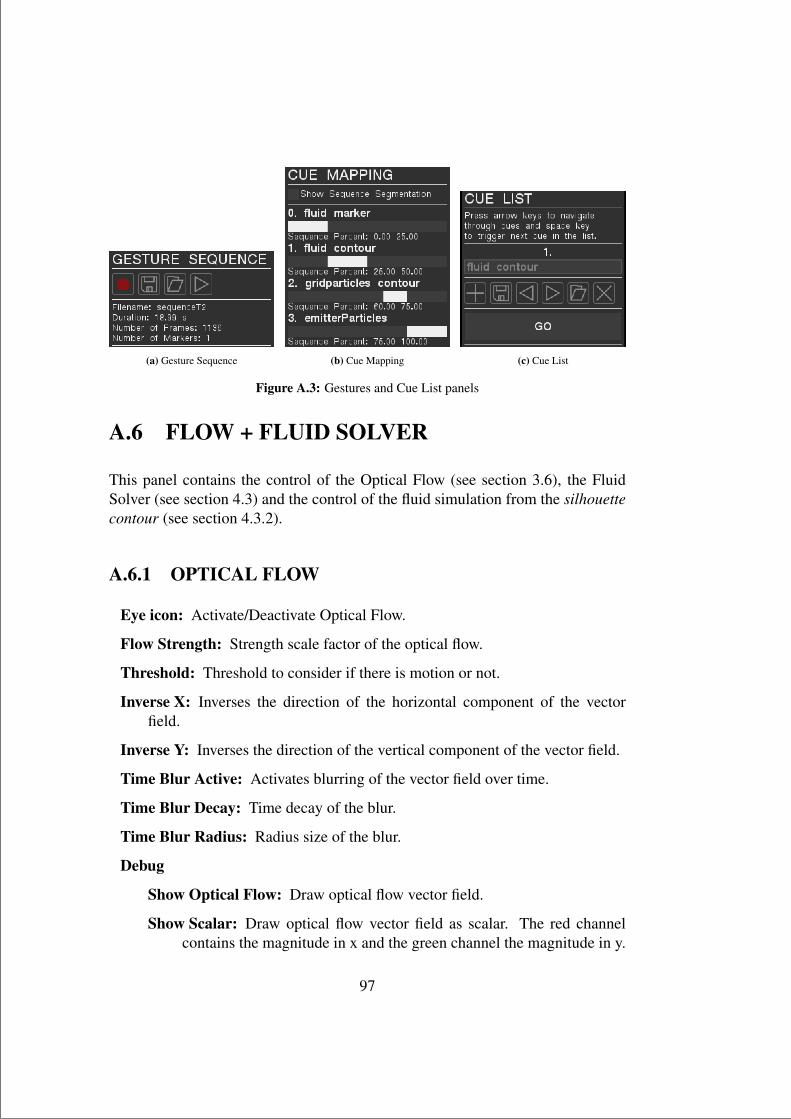
“main” — 2015/7/9 — 12:18 — page 97 — #111

(a) Gesture Sequence (b) Cue Mapping (c) Cue List

Figure A.3: Gestures and Cue List panels

A.6 FLOW + FLUID SOLVER

This panel contains the control of the Optical Flow (see section 3.6), the FluidSolver (see section 4.3) and the control of the fluid simulation from the silhouettecontour (see section 4.3.2).

A.6.1 OPTICAL FLOW

Eye icon: Activate/Deactivate Optical Flow.

Flow Strength: Strength scale factor of the optical flow.

Threshold: Threshold to consider if there is motion or not.

Inverse X: Inverses the direction of the horizontal component of the vectorfield.

Inverse Y: Inverses the direction of the vertical component of the vector field.

Time Blur Active: Activates blurring of the vector field over time.

Time Blur Decay: Time decay of the blur.

Time Blur Radius: Radius size of the blur.

Debug

Show Optical Flow: Draw optical flow vector field.

Show Scalar: Draw optical flow vector field as scalar. The red channelcontains the magnitude in x and the green channel the magnitude in y.

97

“main” — 2015/7/9 — 12:18 — page 98 — #112

A.6.2 VELOCITY MASK

Mask Strength: Strength of the velocity mask (alpha).

Blur Passes: Number of times we apply Gaussian Blur .

Blur Radius: Radius size of the Gaussian Blur.

Debug

Show Velocity Mask: Draw velocity mask.

Show Velocity Mask Contour: Draw contours detected from velocity mask.

(a) Optical Flow (b) VelocityMask

Figure A.4: Optical Flow and Velocity Mask panels

A.6.3 FLUID SOLVER

Eye icon: Activate/Deactivate Fluid Solver.

Reset Icon: Reset Fluid Solver.

General Red: Sets the red color component of all the fluids.

General Green: Sets the green color component of all the fluids.

General Blue: Sets the blue color component of all the fluids.

General Opacity: Sets the opacity of all the fluids.

IR Marker: Sets the IR Markers as input to the fluid.

98

“main” — 2015/7/9 — 12:18 — page 99 — #113

Contour: Sets the silhouette contour as input to the fluid.

Solver

Speed: Increases delta time between frames so fluid advances faster.

Cell Size: Size of the two-dimensional grid cells that define the fluid space.

Num Jacobi Iterations: Number of Jacobi iterations to converge to the so-lution of the Poisson equations that describe the pressure physics of thefluid.

Viscosity: Resistance of the fluid, known also as “thickness”.

Vorticity: Magnitude of the rotational motions of the fluid.

Dissipation: Decay of the fluid density.

Advanced Dissipation

Velocity Offset: Offset of the ‘Dissipation’ in the advection step of veloc-ity field.

Density Offset: Offset of the ‘Dissipation’ in the advection step of densityfield.

Temperature Offset: Offset of the ‘Dissipation’ in the advection step ofthe temperature field.

Smoke Buoyancy

Sigma: Scalar multiplying the temperature difference. Higher it is the morebuoyancy effect.

Weight: Weight of the smoke.

Ambient Temperature: Ambient temperature of the fluid space.

Gravity X: Horizontal component of the gravity force applied evenly tothe entire fluid.

Gravity Y: Vertical component of the gravity force applied evenly to theentire fluid.

Maximum

Clamp Force: Maximum force magnitude limit.

Density: Maximum density limit.

Velocity: Maximum velocity magnitude limit.

99

“main” — 2015/7/9 — 12:18 — page 100 — #114

Temperature: Maximum temperature limit.

Density From Pressure: Multiply fluid density by pressure. This sets the forceof the pressure field.

Density From Vorticity: Multiply fluid density by vorticity. This sets the forceof the vorticity field

Debug

Show Fluid Velocities: Draw fluid vector field.

Show Fluid Velocities Scalar: Draw fluid vector field as scalar. The redchannel contains the magnitude in x and the green channel the magni-tude in y.

Show Pressure: Draw pressure scalar.

Show Temperature: Draw temperature scalar.

Show Vorticity Confinement: Draw vorticity confinement field as scalar.

A.6.4 FLUID CONTOUR

Eye icon: Activate/Deactivate Fluid coming from the silhouette contour.

Red: Sets the red channel of the injected fluid.

Green: Sets the green channel of the injected fluid.

Blue: Sets the blue channel of the injected fluid.

Opacity: Sets the opacity of the injected fluid.

Random colors: Randomizes fluid color over time.

A.7 FLUID 2 + CONTOUR

This panel contains the control of the fluid simulation from the IR Markers (seesection 4.3.2), Fluid Particles (see section 4.4.8) and the different Silhouette Rep-resentation possibilities (see section 4.5).

100

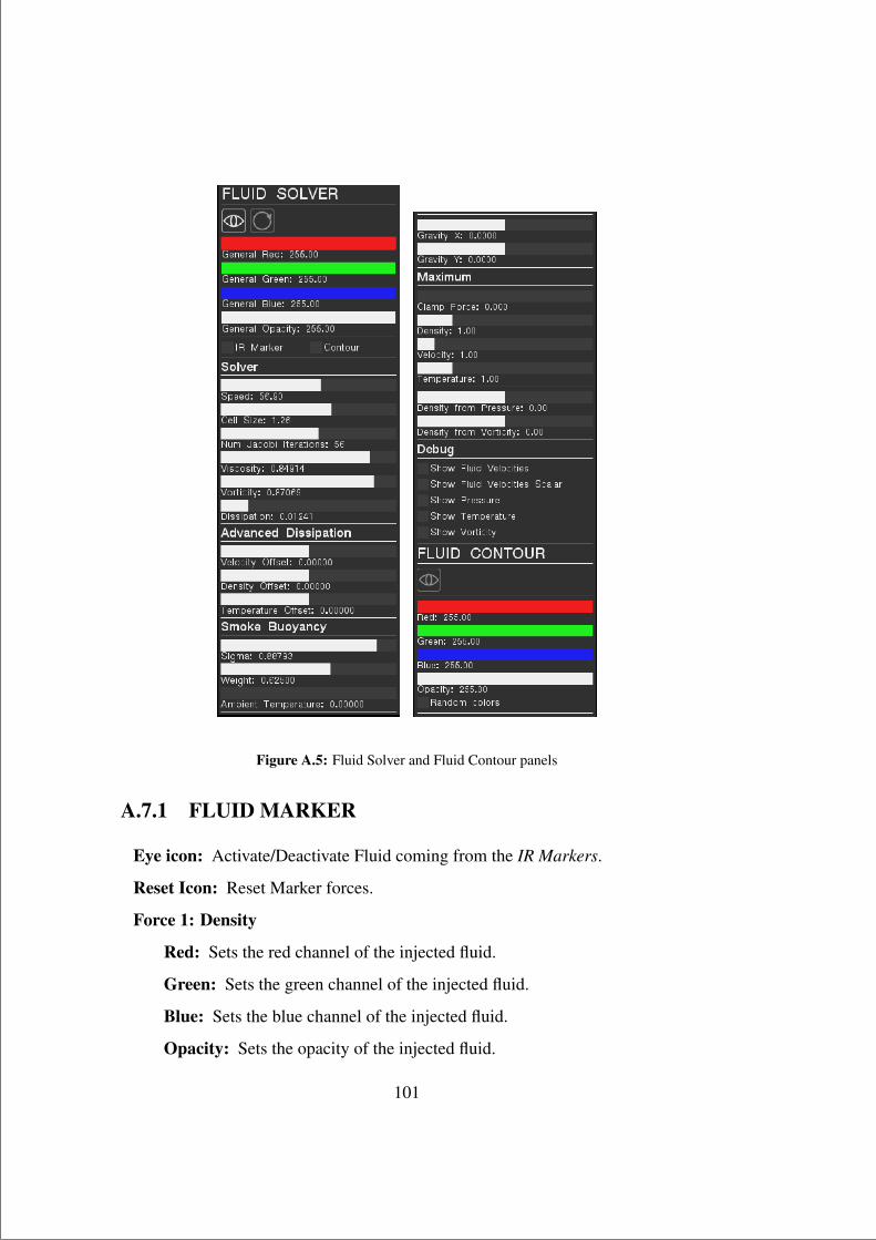
“main” — 2015/7/9 — 12:18 — page 101 — #115

Figure A.5: Fluid Solver and Fluid Contour panels

A.7.1 FLUID MARKER

Eye icon: Activate/Deactivate Fluid coming from the IR Markers.

Reset Icon: Reset Marker forces.

Force 1: Density

Red: Sets the red channel of the injected fluid.

Green: Sets the green channel of the injected fluid.

Blue: Sets the blue channel of the injected fluid.

Opacity: Sets the opacity of the injected fluid.

101

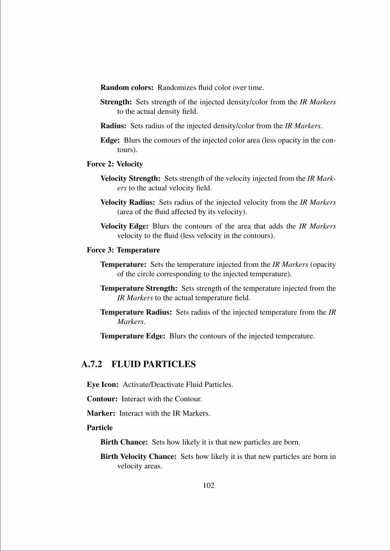
“main” — 2015/7/9 — 12:18 — page 102 — #116

Random colors: Randomizes fluid color over time.

Strength: Sets strength of the injected density/color from the IR Markersto the actual density field.

Radius: Sets radius of the injected density/color from the IR Markers.

Edge: Blurs the contours of the injected color area (less opacity in the con-tours).

Force 2: Velocity

Velocity Strength: Sets strength of the velocity injected from the IR Mark-ers to the actual velocity field.

Velocity Radius: Sets radius of the injected velocity from the IR Markers(area of the fluid affected by its velocity).

Velocity Edge: Blurs the contours of the area that adds the IR Markersvelocity to the fluid (less velocity in the contours).

Force 3: Temperature

Temperature: Sets the temperature injected from the IR Markers (opacityof the circle corresponding to the injected temperature).

Temperature Strength: Sets strength of the temperature injected from theIR Markers to the actual temperature field.

Temperature Radius: Sets radius of the injected temperature from the IRMarkers.

Temperature Edge: Blurs the contours of the injected temperature.

A.7.2 FLUID PARTICLES

Eye Icon: Activate/Deactivate Fluid Particles.

Contour: Interact with the Contour.

Marker: Interact with the IR Markers.

Particle

Birth Chance: Sets how likely it is that new particles are born.

Birth Velocity Chance: Sets how likely it is that new particles are born invelocity areas.

102

“main” — 2015/7/9 — 12:18 — page 103 — #117

Lifetime: Lifetime of the particles.

Lifetime Random: Randomness of the lifetime of the particles.

Mass: Mass of the particles.

Mass Random: Randomness of the mass of the particles.

Size: Radius of the particles.

Size Random: Randomness of the radius of the particles.

A.7.3 SILHOUETTE CONTOUR

Eye Icon: Activate/Deactivate Depth Contour.

Red: Sets the red color component of the contour.

Green: Sets the green color component of the contour.

Blue: Sets the blue color component of the contour.

Opacity: Sets the opacity of the contour.

Contours

Bounding Rectangle: Draw bounding rectangle.

Bounding Rectangle Line: Draw bounding rectangle line contour.

Convex Hull: Draw Convex Hull.

Convex Hull Line: Draw Convex Hull line contour.

Silhouette: Draw Silhouette.

Silhouette Line: Draw silhouette contour line.

Smoothing Size: Smoothing size of the silhouette contour.

Line Width: Width of the contour line.

Scale: Scaling factor of the overall contour.

Debug

Show Contour Velocities: Draw velocities detected from computing dif-ference in contour between two consecutive frames (not being used).

103

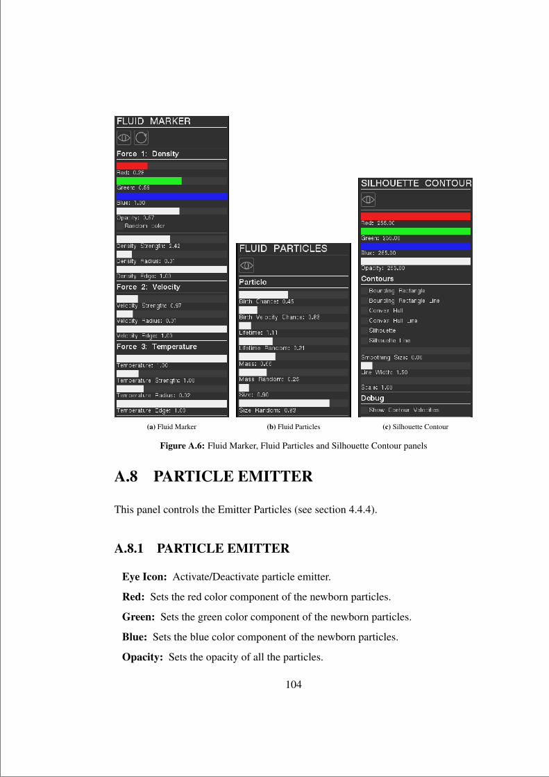
“main” — 2015/7/9 — 12:18 — page 104 — #118

(a) Fluid Marker (b) Fluid Particles (c) Silhouette Contour

Figure A.6: Fluid Marker, Fluid Particles and Silhouette Contour panels

A.8 PARTICLE EMITTER

This panel controls the Emitter Particles (see section 4.4.4).

A.8.1 PARTICLE EMITTER

Eye Icon: Activate/Deactivate particle emitter.

Red: Sets the red color component of the newborn particles.

Green: Sets the green color component of the newborn particles.

Blue: Sets the blue color component of the newborn particles.

Opacity: Sets the opacity of all the particles.

104

“main” — 2015/7/9 — 12:18 — page 105 — #119

IR Marker: Sets the IR Markers as emitting and interacting source.

Contour: Sets the silhouette contours as emitting and interacting source.

Emitter

Particles/sec: Controls how many particles are born every second.

Velocity: Sets the initial velocity of newborn particles.

Velocity Random[ % :] Adds randomness to the initial velocity of new-born particles.

Velocity from Motion[ % :] Lets the particles take the velocity from theinput source (IR Marker velocity or silhouette contour optical flow).Negative values makes the particles move opposite to how the inputsource moves, giving a feel of a ‘jet’ spray.

Emitter Size: Increases the area from where particles are emitted.

Emit all time: Born particles all the time.

Emit all time on contour: Born particles all the time but only on the con-tour shape.

Emit only if movement: Born particles only if there is enough movement.

Physics

Friction: Makes particles velocity decrease over time.

Gravity X: Adds gravity in the horizontal direction.

Gravity Y: Adds gravity in the vertical direction.

Turbulence: Adds noise affecting the motion of the particles.

Bounces: Makes the particles bounce with the boundaries of the window.

Steers: Makes the particles steer away before hitting the boundaries of thewindow.

Infinite: Makes infinite boundaries.

Repulse: Makes particles repulse from each other.

Repulse Dist: Sets the repulsion distance between particles.

Particle

Empty: Draws empty particles, just the contour line.

105

“main” — 2015/7/9 — 12:18 — page 106 — #120

Line: Draws a line instead of a circle.

Stroke: Draws a black contour stroke around the particles.

Stroke Line Width: Sets the line width of the stroke.

Connected: Draws a line connecting particles that are closer than Con-nected Dist.

Connected Dist: Sets the maximum distance between particles to be con-nected.

Connected Line Width: Sets the line width of the connecting line.

Lifetime: Controls how long the particles live.

Life Random[ % :] Adds randomness to the lifetime of particles.

Radius: Sets radius size of the particles.

Radius Random[ % :] Adds randomness to the radius size of the particles.

Time Behavior

Size: Decrease particle size over its lifespan.

Alpha: Decrease particle opacity over its lifespan.

Flickers: Make particle flicker before dying.

Color: Change particle color over its lifespan.

Interaction

Interact: Makes the particles interact with the input source.

Interaction Radius: Sets the radius of the interaction area.

Interaction Force: Sets the force of interaction.

Flow Interaction: Make optical flow and IR Markers velocities affect par-ticles motion.

Fluid Interaction: Make fluid velocities affect particles motion.

Seek Interaction: Make particles seek markers position (only works for IRMarker input).

Gravity Interaction: Make particles that are “touched” fall in a naturalway.

Attract Interaction: Make particles attract to input source.

106

“main” — 2015/7/9 — 12:18 — page 107 — #121

Repulse Interaction: Make particles repulse from input source.

Bounce Interaction: Make particles bounce from silhouette contour (onlyworks for Contour input).

Figure A.7: Emitter Particles panel

A.9 PARTICLE GRID

This panel controls the Grid Particles (see section 4.4.5).

Eye Icon: Activate/Deactivate particle emitter.

Red: Sets the red color component of the newborn particles.

107

“main” — 2015/7/9 — 12:18 — page 108 — #122

Green: Sets the green color component of the newborn particles.

Blue: Sets the blue color component of the newborn particles.

Opacity: Sets the opacity of all the particles.

IR Marker: Sets the IR Markers as interacting source.

Contour: Sets the silhouette contours as interacting source.

Grid

Resolution: Resolution of the grid (width/resolution x height/resolution).

Particle

Empty: Draws empty particles, just the contour line.

Line: Draws a line instead of a circle.

Stroke: Draws a black contour stroke around the particles.

Stroke Line Width: Sets the line width of the stroke.

Connected: Draws a line connecting particles that are closer than Con-nected Dist.

Connected Dist: Sets the maximum distance between particles to be con-nected.

Connected Line Width: Sets the line width of the connecting line.

Radius: Sets radius size of the particles.

Physics

Friction: Makes particles velocity decrease over time.

Return to Origin: Make particles return to its original position.

Return to Origin Force: Force of making particles return to its originalposition.

Repulse: Makes particles repulse from each other.

Repulse Dist: Sets the repulsion distance between particles.

Interaction

Interact: Makes the particles interact with the input source.

Interaction Radius: Sets the radius of the interaction area.

108

“main” — 2015/7/9 — 12:18 — page 109 — #123

Interaction Force: Sets the force of interaction.

Flow Interaction: Make optical flow and IR Markers velocities affect par-ticles motion.

Fluid Interaction: Make fluid velocities affect particles motion.

Seek Interaction: Make particles seek markers position (only works for IRMarker input).

Gravity Interaction: Make particles that are “touched” fall in a naturalway.

Attract Interaction: Make particles attract to input source.

Repulse Interaction: Make particles repulse from input source.

A.10 PARTICLE BOIDS

This panel controls the Boids Particles (see section 4.4.6).

Eye Icon: Activate/Deactivate particle emitter.

Red: Sets the red color component of the newborn particles.

Green: Sets the green color component of the newborn particles.

Blue: Sets the blue color component of the newborn particles.

Opacity: Sets the opacity of all the particles.

IR Marker: Sets the IR Markers as interacting source.

Contour: Sets the silhouette contours as interacting source.

Flocking

Number of particles: Number of particles born at once.

Flocking Radius: Distance at which the boids are considered flockmates.

Lower Threshold: Threshold that determines if boids get separated or aligned.

Higher Threshold: Threshold that determines if boids get aligned or at-tracted.

Max Speed: Maximum speed of the boids.

Separation Strength: Strength of the separation force.

109

“main” — 2015/7/9 — 12:18 — page 110 — #124

Attraction Strength: Strength of the attraction force.

Alignment Strength: Strength of the alignment force.

Physics

Friction: Makes particles velocity decrease over time.

Gravity X: Adds gravity in the horizontal direction.

Gravity Y: Adds gravity in the vertical direction.

Turbulence: Adds noise affecting the motion of the particles.

Bounces: Makes the particles bounce with the boundaries of the window.

Steers: Makes the particles steer away before hitting the boundaries of thewindow.

Infinite: Makes infinite boundaries.

Particle

Empty: Draws empty particles, just the contour line.

Line: Draws a line instead of a circle.

Stroke: Draws a black contour stroke around the particles.

Stroke Line Width: Sets the line width of the stroke.

Connected: Draws a line connecting particles that are closer than Con-nected Dist.

Connected Dist: Sets the maximum distance between particles to be con-nected.

Connected Line Width: Sets the line width of the connecting line.

Radius: Sets radius size of the particles.

Radius Random[ % :] Adds randomness to the radius size of the particleswhen born.

Interaction

Interact: Makes the particles interact with the input source.

Interaction Radius: Sets the radius of the interaction area.

Interaction Force: Sets the force of interaction.

110

“main” — 2015/7/9 — 12:18 — page 111 — #125

Flow Interaction: Make optical flow and IR Markers velocities affect par-ticles motion.

Fluid Interaction: Make fluid velocities affect particles motion.

Seek Interaction: Make particles seek markers position (only works for IRMarker input).

Gravity Interaction: Make particles that are “touched” fall in a naturalway.

Attract Interaction: Make particles attract to input source.

Repulse Interaction: Make particles repulse from input source.

Bounce Interaction: Make particles bounce from silhouette contour (onlyworks for Contour input).

A.11 PARTICLE ANIMATIONS

This panel controls the Animations Particles (see section 4.4.7).

Eye Icon: Activate/Deactivate particle emitter.

Red: Sets the red color component of the newborn particles.

Green: Sets the green color component of the newborn particles.

Blue: Sets the blue color component of the newborn particles.

Opacity: Sets the opacity of all the particles.

IR Marker: Sets the IR Markers as interacting source.

Contour: Sets the silhouette contours as interacting source.

Animation

Rain: Set Rain animation.

Snow: Set Snow animation.

Explosion: Set Explosion animation.

Rain and Snow

Particles/sec: Controls how many particles are born every second.

Explosion

111

“main” — 2015/7/9 — 12:18 — page 112 — #126

Number of particles: Number of particles born at once.

Interaction

Interact: Makes the particles interact with the input source.

Interaction Radius: Sets the radius of the interaction area.

Interaction Force: Sets the force of interaction.

Flow Interaction: Make optical flow and IR Markers velocities affect par-ticles motion.

Fluid Interaction: Make fluid velocities affect particles motion.

Seek Interaction: Make particles seek markers position (only works for IRMarker input).

Gravity Interaction: Make particles that are “touched” fall in a naturalway.

Attract Interaction: Make particles attract to input source.

Repulse Interaction: Make particles repulse from input source.

Bounce Interaction: Make particles bounce from silhouette contour (onlyworks for Contour input).

Particle

Empty: Draws empty particles, just the contour line.

Line: Draws a line instead of a circle.

Stroke: Draws a black contour stroke around the particles.

Stroke Line Width: Sets the line width of the stroke.

Connected: Draws a line connecting particles that are closer than Con-nected Dist.

Connected Dist: Sets the maximum distance between particles to be con-nected.

Connected Line Width: Sets the line width of the connecting line.

Lifetime: Controls how long the particles live.

Life Random[ % :] Adds randomness to the lifetime of particles.

Radius: Sets radius size of the particles.

112

“main” — 2015/7/9 — 12:18 — page 113 — #127

Radius Random[ % :] Adds randomness to the radius size of the particles.

Physics

Friction: Makes particles velocity decrease over time.

Gravity X: Adds gravity in the horizontal direction.

Gravity Y: Adds gravity in the vertical direction.

Turbulence: Adds noise affecting the motion of the particles.

Bounces: Makes the particles bounce with the boundaries of the window.

Steers: Makes the particles steer away before hitting the boundaries of thewindow.

Infinite: Makes infinite boundaries.

Repulse: Makes particles repulse from each other.

Repulse Dist: Sets the repulsion distance between particles.

113

“main” — 2015/7/9 — 12:18 — page 114 — #128