design and implementation of a high-speed solid-state
TRANSCRIPT

Design and Implementation of a High-Speed Solid-State
Acousto-Optic Interference Pattern Projector for
Three-Dimensional Imaging
by
Daniel L. Feldkhun
Submitted to the Department of Electrical Engineering and Computer Science
in partial fulfillment of the requirements for the degree of
Master of Engineering in Electrical Engineering and Computer Science
at the
Massachusetts Institute of Technology
Spring 1999
@ Copyright 1999 Daniel L. Feldkhun. All rights reserved.
The author hereby grants to M.I.T. permission to reproduce and MAdistribute publicly paper and electronic copies of this thesis
and to grant others the right to do so.
Department of Electrical Engineering and Computer ScienceSpring, 1999
Certified by(Y Lyle G. Shirley
MIT Lincoln Laboratory Research Staff
( I >*
_,_Aesis Supervisor
Certified byDennis Freeman
ciate Professo in Ele trical EngineeringThesis-Supervisor
Accepted byArthur C. Smith
Chairman, Department Committee on Graduate Theses
/
Nof
f- ,, 4 __ -

Design and Implementation of a High-Speed Solid-State
Acousto-Optic Interference Pattern Projector for
Three-Dimensional Imaging
by
Daniel L. Feldkhun
Submitted To The Department Of Electrical Engineering And Computer Science
Spring 1999
In Partial Fulfillment Of The Requirements For The Degree OfMaster Of Engineering In Electrical Engineering And Computer Science
Abstract
A novel method of projecting interference patterns using acousto-optics has beendeveloped and implemented in the context of the Accordion Fringe Interferometry (AFI)three-dimensional measurement technique developed at MIT Lincoln Laboratory. AFI isan active technique that relies on projecting interference fringes and triangulation torecover range information. AFI is suitable for a wide range of applications, and the solid-state acousto-optic interference fringe projector offers the combination of speed,robustness, and portability that can make AFI a very powerful tool for applications likemachine vision, hand-held 3D scanning, high-throughput quality control systems, andmotion study and modeling. This work presents the theory of acousto-optic devices andaddresses design considerations for an acousto-optic AFI system. Moreover, a prototypeis constructed and evaluated, and an algorithm is implemented to reconstruct the 3Dsurface of an object. The results indicate that an acousto-optic AFI system is practicaland has high potential for applications that require high speed and portability from a 3Dimaging system.
Thesis Supervisor: Lyle G. ShirleyTitle: MIT Lincoln Laboratory Research Staff
Thesis Supervisor: Dennis M. FreemanTitle: Associate Professor in Electrical Engineering
2
Acknowledgements
I would like to thank everyone at the Laser Speckle Lab for creating a friendly and
pleasant atmosphere to work in. I'd like to thank Dr. Shirley for his continued direction
and his support in my accelerated quest to graduate. I am also in debt to Prof. Freeman
who despite a plethora of theses, conferences, and management responsibilities, has taken
time to offer help and advice when I needed it the most. I thank Michael Mermelstein for
his invaluable counsel and creativity throughout this project and for all he has taught me
about life, science, and the pursuit of happiness. I would also like to thank my parents for
believing in me and providing much needed emotional support and inspiration. Finally, I
am grateful to MIT Lincoln Laboratory and the MIT Department of Electrical
Engineering and Computer Science for supporting me in the course of this work.
3

Table of Contents
1 INTRODUCTION......................................................................................................................................7
1.1 MOTIVATIONS FOR DEVELOPING A HIGH-SPEED THREE DIMENSIONAL IMAGER .................................. 7
1.2 BRIEF SURVEY OF 3D IMAGING TECHNIQUE ..................................................................................... 10
1.3 BACKGROUND OF THE LASER SPECKLE LABORATORY....................................................................... 13
2 ACCORDION FRINGE INTERFEROMETRY............................................................................... 15
2.1 "PAINTING THE WORLD WITH FRINGES ........................................................................................... 15
2.2 DEPTH EXTRACTION THROUGH SPATIAL PHASE ESTIMATION............................................................... 18
2.3 DEPTH EXTRACTION THROUGH SPECTRAL ESTIMATION.......................................................................21
2.4 B EN EFITS O F A FI ................................................................................................................................ 23
2.5 C URRENT STATE O F A FI...................................................................................................................... 24
3 IMPLEMENTATION OF AFI PROJECTOR USING ACOUSTO-OPTICS ............................... 25
3.1 PHYSICS OF AN ACOUSTO-OPTIC MODULATOR............................................................................... 25
3.2 GENERATING STATIONARY INTERFERENCE FRINGE PATTERNS ....................................................... 32
3.2.1 Projecting accordion fringes .................................................................................................. 32
3.2.2 F reezing the fringes ................................................................................................................... 34
3.3 AN IMPLEMENTATION OF AN ACOUSTO-OPTIC PROJECTOR ............................................................... 41
3.3.1 Target A pp lication......................................................................................................................4 1
3.3.2 System desig n ............................................................................................................................. 42
3 .3 .3 R esu lts ........................................................................................................................................ 5 7
3.4 BENEFITS OF THE ACOUSTO-OPTIC PROJECTOR...................................................................................60
4 DEPTH-RETRIEVAL FOR STATIONARY AND MOVING TARGETS....................................64
4.1. ALGORITHM FOR DEPTH RETRIEVAL USING SPATIAL PHASE ESTIMATION ....................................... 64
4

4.1.1 Triangulation..............................................................................................................................64
4.1.2 Phase Unwrapping ..................................................................................................................... 67
4.2 M EASUREMENTS AND RESULTS ....................................................................................................... 69
5 CO NCLUSIONS ...................................................................................................................................... 77
APPENDIX A: AN IMPLEMENTATION OF THE AFI ALGORITHM...................82
BIBLIO G RAPH Y ....................................................................................................................................... 86
5
List of Figures
FIGURE 1.1 EXAMPLE APPLICATIONS FOR HIGH-SPEED 3D IMAGING ........................................................... 9
F IG URE 2.1 FR ING E SPACE............................................................................................................................ 16
FIGURE 2.2 MAPPING FRINGES TO DEPTH USING SPATIAL PHASE ESTIMATION .............................................. 19
FIGURE 2.3 ESTIMATING SPATIAL PHASE BY PHASE-SHIFTING THE FRINGES ± 90 .................................... 20
FIGURE 2.4 PRINCIPLE OF PHASE UNWRAPPING USING LARGER REFERENCE FRINGES................................ 20
FIGURE 2.5 MAPPING FRINGES TO DEPTH USING SPECTRAL ESTIMATION .................................................. 22
FIGURE 3.1 THE BRILLOUIN PHENOMENON IN A BRAGG CELL .................................................................. 26
FIGURE 3.2 BEAM DEFLECTION USING AN ACOUSTO-OPTIC CELL .............................................................. 31
FIGURE 3.3 A COMPOUND-DRIVE ACOUSTO-OPTIC FRINGE PROJECTOR ..................................................... 33
FIGURE 3.4 FREEZING AND PHASE SHIFTING A TRAVELING INTERFERENCE PATTERN................................ 36
FIGURE 3.5 USING PERIODIC CONVOLUTION TO MODEL FRINGE INTENSITY .............................................. 38
FIGURE 3.6 ELEMENTS OF LABORATORY ACOUSTO-OPTIC AFI SETUP ...................................................... 43
FIGURE 3.7 ACOUSTO-O PTIC AFI SETUP.................................................................................................... 44
FIGURE 3.8 GAUSSIAN BEAM PROPAGATION............................................................................................ 51
FIGURE 3.9 RESULTS: 30MHZ FRINGES ON A SPRAY-PAINTED GOLF BALL .............................................. 58
F IG URE 4.1 T RIA NG U LAT IO N ........................................................................................................................ 66
FIGURE 4.2 PHASE UNW RAPPING .................................................................................................................. 68
FIGURE 4.3 SIMULATIONS SHOW ALGORITHM CORRECTNESS ........................................................................ 70
FIGURE 4.4 FROM FRINGES To PHASEMAPS ............................................................................................. 71
FIGURE 4.5 3D RECONSTRUCTION OF THE ILLUMINATED SURFACE OF A GOLF BALL..................................72
FIGURE 4.6 RECONSTRUCTION OF A LEGOM STUB USING ONLY SIx CCD FRAMES ................................... 76
FIGURE 5.1 RF DRIVE ELECTRONICS USING QUALCOMM Q2368 DDS INTEGRATED CIRCUIT ...................... 79
6

Chapter 1
Introduction
1.1 Motivations for developing a high-speed three dimensional imager
The electronic age has revolutionized our ability to learn and communicate.
While humans have long known how to write manuscripts and draw pictures, the amount
of information that we can now record and express using audio and video technologies is
unprecedented. Furthermore, the advents of telephone, radio, television, and data
communications networks, have made access to such information increasingly integral to
our lives. Computers are rapidly increasing our capacity to store, process, and digest this
information.
As desktop computing power is skyrocketing, it is becoming ever easier to
visualize three-dimensional objects without having to leave our chairs. Whether it is a
building or a bug, with a click of a button we can view it from any angle, choose any
desired lighting environment, zoom into any crevice, and explore the object much quicker
and more thoroughly than two-dimensional images, or even movies, ever allowed. When
it comes to recording the three-dimensional world, however, for the most part we are still
7
at the level of a painter or a scribe. While 3D imaging tools are available in narrow
circles, they are often costly, cumbersome, and slow to use.
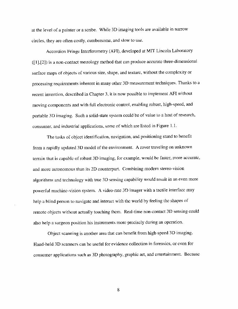
Accordion Fringe Interferometry (AFI), developed at MIT Lincoln Laboratory
([1],[2]) is a non-contact metrology method that can produce accurate three-dimensional
surface maps of objects of various size, shape, and texture, without the complexity or
processing requirements inherent in many other 3D measurement techniques. Thanks to a
recent invention, described in Chapter 3, it is now possible to implement AFI without
moving components and with full electronic control, enabling robust, high-speed, and
portable 3D imaging. Such a solid-state system could be of value to a host of research,
consumer, and industrial applications, some of which are listed in Figure 1.1.
The tasks of object identification, navigation, and positioning stand to benefit
from a rapidly updated 3D model of the environment. A rover traveling on unknown
terrain that is capable of robust 3D imaging, for example, would be faster, more accurate,
and more autonomous than its 2D counterpart. Combining modem stereo-vision
algorithms and technology with true 3D sensing capability would result in an even more
powerful machine-vision system. A video-rate 3D imager with a tactile interface may
help a blind person to navigate and interact with the world by feeling the shapes of
remote objects without actually touching them. Real-time non-contact 3D sensing could
also help a surgeon position his instruments more precisely during an operation.
Object scanning is another area that can benefit from high-speed 3D imaging.
Hand-held 3D scanners can be useful for evidence collection in forensics, or even for
consumer applications such as 3D photography, graphic art, and entertainment. Because
8

High-Speed 3D
Objectives -
Applications
Object Identification,
Navigation
Positioning
Machine Vision
Sensory Aid
Surgery
Object Scanning
hand-held high-thr
Evidence Collection
3D "Photography"
Graphic Art
oughput
Conveyor-Belt QC
3D Security Video
Motion Study
Modeling
Failure Prediction
Speech Recognition
Stress Analysis
Anatomy Studies
Figure 1.1 Example applications for high-speed 3D imaging
hand-held devices tend to shake, fast acquisition times are necessary. Other applications,
such as quality control on a factory conveyor belt, look at moving objects and require
high throughput from the 3D imaging system. Law enforcement is another possible
application in which 3D reconstruction of faces, property, and crime scenes can be
helpful.
The study and modeling of motion is important in a number of research areas. An
accurate 3D model of a person's lips during speech can offer additional insight for lip
reading and speech recognition research and applications [3]. As another example, 3D
visualization of surface distortions in an object under varying stress, can be used to
predict and analyze failure modes of a complex mechanical system.
1.2 Brief survey of 3D imaging technique
Although there are relatively few 3D measurement systems in production, there is
a plethora of 3D measurement techniques present in the literature [4]. First, one must
differentiate between contact and non-contact techniques. Contact 3D measurement
devices, such as the Coordinate Measuring Machine (CMM), rely on physically probing
the surface of an object. Although CMMs are common in industry, these highly accurate
machines are generally very slow, cumbersome, and limited in the extent and nature of
the objects they can measure. Of more relevance to this thesis work are non-contact
techniques which analyze the reflected light from a distant target.
Non-contact direct 3D measurement techniques can be either active or passive
and rely on either triangulation or time-of-flight to determine the depth of the target [5].
10

Passive techniques rely on ambient light reflected from the surface of an object. Stereo
vision is a familiar example of a passive triangulation-based method, where the distance
to a point in space viewed from different angles by two detectors can be determined using
the law of cosines. Although humans are very adept at using stereo vision to perceive the
3D world, this task is much more daunting for machines. At the heart of the matter is the
correspondence problem: the difficulty of reliably matching points in the two stereo
images. This task requires highly intelligent (and compute-intensive) algorithms, that
rely on high-contrast features in the images, and can be easily confused by angle-
dependent variation of surface reflectance of the object.
Active triangulation-based techniques solve the correspondence problem by
projecting structured light onto the object. In this case, since the spatial distribution of
the illumination is known, only a single detector is necessary to triangulate the position of
a given illuminated point. A simple example of a structured light technique is point
triangulation, where a focused laser beam is serially scanned across the object [6]. Since
the laser beam direction relative to the detector is known at any instant of time, the 3D
location of the illuminated point can be determined. Other structured light techniques
project more complex patterns to parallelize the measurement process, using cylindrical
lenses, slits, or even coded masks on a slide projector. Related to the AFI technique
discussed in this thesis, is the Moird Interferometry method [7]. Moir6 Interferometry
relies on two identical gratings, one at the source and one at the detector to superimpose
an interference fringe pattern onto the image of the object. The phase of these fringes can
be unwrapped via image processing and used to extract the depth of the object via
triangulation. All structured light techniques, however, suffer from the problem of
11
specular reflection. A mirror-like surface, for example, may direct the projected light
away from the detector, resulting in no data, or worse, deflect the light onto other areas
on the surface, resulting in an erroneous measurement. In addition, many active
techniques rely on mechanically scanning laser beams or patterns, and are slow as a
result. Furthermore, common to all triangulation techniques is the problem of missing
data that results from shadowing. While shadowing can be reduced by shortening the
baseline between the two triangulation elements, this also results in increased
measurement errors.
Time-of-flight techniques, on the other hand, avoid the missing data problem by
co-locating the detector and the projector. The most straight-forward time-of-flight
technique measures the round-trip time of a reflected laser pulse, although the high
temporal resolution required from the detector and the associated electronics makes such
range-finders expensive and typically limits the resolution to a few centimeters.
Continuous-wave time-of-flight approaches that rely on amplitude or frequency
modulation also exist and greatly improve on this resolution. However, phase ambiguity
problems and long exposure times necessary to reduce photon noise currently limit the
range of applications for such techniques [5] .
A host of indirect 3D measurement methods also exist that obtain the relative
shape of the object, not an absolute depth measurement. These techniques typically rely
on cues like reflectance properties of the object, focus of the image, perspective, or
texture gradients, and generally work for only a narrow range of objects and
environments.
12

Despite the abundance of 3D measurement techniques, no prominent versatile
approach suited for a wide range of applications has so far emerged. Accordion Fringe
Interferometry, developed at MIT Lincoln Laboratory, is a structured light technique that
has been used to reconstruct surfaces of objects in a wide range of sizes, shapes, and
textures. It is also robust against errors, simple to implement, inexpensive, and can be
made portable and fast with the technology presented in this work.
1.3 Background of the Laser Speckle Laboratory
Much of this thesis represents work done at the Laser Speckle Laboratory, part of
Group 35 of the MIT Lincoln Laboratory. The Laser Speckle Lab (LSL), which was
formed in 1990 under the leadership of Dr. Lyle Shirley, develops novel measurement
techniques using patterns produced by interference of coherent light. While its initial
work was aimed at laser speckle pattern sampling ([8], [9],[10],[1 1]) for target
identification in missile defense, in recent years the group's focus evolved towards three-
dimensional industrial metrology applications. A number of interferometric methods
have developed in the process, with Accordion Fringe Interferometry (AFI) ([1],[2])
representing the latest, simplest, and perhaps most promising non-contact technique for
acquiring three-dimensional surface maps of opaque objects.
In its latest incarnation, the AFI system at LSL has proven to be of high interest to
the automotive and aeroplane industries for measuring large panels in process control.
Such applications require a highly robust, large-scale system, capable of micron-scale
resolution over a large area of coverage. There are a host of other applications, however,
that do not require the high resolution or the large scale of an industrial apparatus, but
13

stand to benefit from the simplicity and low processing requirements of AFI. This thesis
represents an effort to adapt the AFI technique to areas in research and medicine that
would benefit from a high-speed, portable, and economical 3D imaging system.
14

Chapter 2
Accordion Fringe Interferometry
2.1 "Painting the world with fringes"
Accordion Fringe Interferometry ([1],[2]) is related to the category of 3D
triangulation methods that rely on projecting "structured light" onto the target. Like the
majority of structured light techniques, AFI requires only a single detector to triangulate
range information about the illuminated target, whereas stereo triangulation systems need
to match images from several detectors, and as a result rely on complex shape recognition
algorithms that are sensitive to angle-dependent reflectivity of the target [5].
However, unlike most structured light methods which generate patterns using
masks at the focal plane or using light-shaping optics, AFI relies on the interference of
coherent light to "paint the world with interference fringes". As illustrated in Figure 2.1,
two laser beams are focused by a lens into two "source points" at the focal plane. After
the focal plane, the two beams diverge and eventually overlap to form the sinusoidal
interference pattern. The density of the interference fringes projected onto a given plane
15

-R4d~
a
2 tan(#i) agI 0 -o @ |
AI
Figure 2.1 Fringe Space
16

in this "fringe space" depends on the distance of the plane from the focal plane and on the
spatial separation of the two source points:
d 2.Ra
Here d is the spacing of the fringes, A is the optical wavelength, R is the distance from the
focal plane to the given interference plane, and a is the separation of the two source
points. The spatial phase of the global fringe pattern can also be varied by changing the
relative phase 9 of the two interfering laser beams. In fact, the intensity at a given point
in the fringe space can be represented by a raised cosine function [12]:
I= 10 .Cos 2 tan(p)-a -r + 0 + Ic
where 6 is defined in the diagram, Io is the amplitude of the fringe pattern, and IDc is the
fixed background illumination level. Note that both Io and IDC will change as the laser
light intensity, background illumination level, and surface reflectivity vary across the
object, and as the path difference between the interfering beams approaches the
coherence length of the laser light. The raised cosine term in the equation, however,
depends only on the location in the fringe space and on the controllable parameters of the
AFI system.
The following sections describe two related ways of extracting depth information
about a given point in the fringe space. Both approaches recover the angular coordinate
#, and use triangulation to determine the distance from the detector to the imaged point.
Spatial phase estimation relies on measuring the local spatial phase # of the fringe pattern
17

at a fixed point source separation a. Spectral estimation looks at the local intensity
variation as the point-source separation a is changed.
2.2 Depth extraction through spatial phase estimation
As shown in Figure 2.2, by measuring the wrapped phase of the fringe pattern
imaged by a pixel in a CCD array (900 in this case), one can isolate several discrete
locations along the line of sight of the pixel where the imaged region of the object might
lie. One way of determining the spatial phase at a given pixel is shown in Figure 2.3. As
information theory dictates, by taking three measurements of a sinusoid of known
frequency (determined by the point source separation in this case), one can determine all
three of its unknown parameters - amplitude, offset, and phase (with a 3600 ambiguity).
This can be done robustly by shifting the phase of the entire projected fringe pattern, and
measuring the corresponding intensities at each pixel independently. As shown in Figure
2.3, an even sampling and a simple formula results from ±90' phase shifts of the fringe
pattern. Since only the spatial phase is of interest for triangulation, the amplitude and
offset parameters are not explicitly calculated.
In order to disambiguate between the possible locations of the imaged point in the
fringe space, we must unwrap the measured phase. One way to achieve this is to project
larger "reference" fringes onto the object. This is shown in Figure 2.4. If a reference
fringe is large enough to cover the entire depth extent of the object, then the phase
measurements with the finer fringes can be completely unwrapped. On the other hand, a
small phase measurement error of a reference fringe that is too large may result in a 360*
phase unwrapping error. Thus, the noise present in the data limits the maximum ratio
18

I = I0 - Cos 2tan( 8)-a -f+
o= 90
/
/
//
II
/I
II
/I
//
I/
/
I
Afv/VV~\
NVW
Figure 2.2 Mapping fringes to depth using spatial phase estimation
19
object
II
/I
/I
//
II
/I
/I
I/
I/
/

Ii --------------
12
13
(x)
'0
IDC
-540* -360* -1800 00 $o 1800 3600 540* 0 (x)
I, = I D o sin #
I2 = IDC+I 0 Cos 00
13 = IDC- 1o sin01
Figure 2.3 Estimating spatial phase by phase-shifting the fringes ± 900
I I i I
-5400 -360* -1800 00 1800I i I
3600 540* (x)
Figure 2.4 Principle of phase unwrapping using larger reference fringes
20
'

between the density of a set of fringes, and the density of the reference fringes used to
unwrap them. Once the fringes are unwrapped, however, they can be used as a reference
to unwrap an even more dense interference pattern. Since finer fringes result in better
resolution', this process can be iterated until the finest fringes are unwrapped.
2.3 Depth extraction through spectral estimation
The concept of spectral estimation in AFI is illustrated in Figure 2.5. Variation in
the separation of the two point-sources causes a stretching of the fringes (as in an
accordion). As required by the raised cosine function, the intensity at any given point in
the fringe space oscillates sinusiodally as a result, where the oscillation frequency is a
function of the angle #. Thus, by determining this oscillation frequency at a given point
on the illuminated object, one can extract its depth via triangulation without ambiguity
(as long as the location of the null fringe is known).
One way to determine the oscillation frequency at a given point is to move the
point-sources apart and count the number of fringes that pass by. This requires hundreds
of image frames for a single surface reconstruction. Another tactic is to use only a few
point source separations, and use a statistical minimization routine to fit a sinusoid to
these samples. This approach, however, can be very computationally-intensive. As a
result of these practical drawbacks, the phase estimation technique was chosen in favor of
spectral estimation (at least at this stage of AFI development).
This is true while the fringes are well enough resolved by the CCD [1].
21

I = 10 -COS
tan(/)
2 ( tan(p) a .r 1+ D
//
/I
I/
I/
I/ -
I/
/I
II/
I/
I/
/
'II
/
a
/ a
Figre2. Mppngfrngs o eph sig petrl stmaio
22

2.4 Benefits of AFI
Accordion Fringe Interferometry extends the state of the art in 3D measurement.
Some of the benefits that AFI has to offer for a wide range of applications including high-
speed and portable 3D imaging are listed below.
* Resistant to propagation of errors: Because phase is calculated and unwrapped for
each pixel independently, errors in range estimation are confined to their
corresponding pixels.
" Well-behaved at sharp edges: Unlike several other 3D techniques which exhibit
discontinuities and other anomalies at sharp edges of the targeted object, AFI is
robust against such discontinuities. Due to the unwrapping process, a phase-
measurement error resulting from a sudden jump within a region imaged by a single
pixel, will be confined to at most 3600. Furthermore, due to the pixel-independent
phase measurement technique, any such errors will not affect neighboring pixels.
e Insensitive to variations in illumination level: Because triangulation depends only on
the phase and frequency of the fringe pattern, variations in amplitude or bias of the
fringe pattern over the extent of the object are inherently compensated for. Although
intensity variations do reduce the dynamic range of the CCD available to some
regions of the object, simulations have shown that the phase estimation technique is
robust even with two or three bits of quantization.
* Parallel acquisition, parallel processing: Because all pixels are acquired
simultaneously by the CCD and range is calculated independently for each pixel, this
technique is fit for parallel processing. Modularity of the steps involved in measuring
and unwrapping the phase also benefit computation efficiency.
23

* Modest processing and memory requirements: The computation involved in
determining and unwrapping the phase for each pixel and performing a triangulation
calculation is comprised of only a few dozen operations. The memory requirements
are also low - at most three CCD frames need to be held in memory at once (during
the phase calculation step). There is a real possibility of real-time video-rate AFI
processing with dedicated hardware.
" Simple hardware: An AFI system consists of a CCD detector, a fringe projector, and
the associated software and electronics. Most of these components are off-the-shelf
items and are relatively economical.
2.5 Current state of AFI
The Accordion Fringe Interferometry technique has evolved through many
iterations of method and prototype. The current AFI system is not only a successful
laboratory prototype, but is being tested at a major airplane production facility to measure
aircraft body panels as part of the quality control process.
One would also like to expand AFI into areas where the requirements are
altogether different from industrial metrology, where more important than high resolution
are low cost, speed, portability, and automation. Clearly, many 3D applications would
benefit from the simplicity and robustness of the AFI method.
A recent invention which provides a solid-state method of projecting and
electronically controlling interference fringes using an Acousto-Optic Modulator may be
instrumental in overcoming the difficulties of bringing AFI into the world of high-speed
portable 3D imaging, perhaps the next big step in its trend of evolution.
24

Chapter 3
Implementation of AFI projector using acousto-optics
Accordion Fringe Interferometry requires precise control over the phase and
frequency of a projected interference fringe pattern. The AFI projector currently used for
industrial metrology relies on translation of optical components, and its precision and
speed is limited by the motion-control system. This chapter presents an alternative solid-
state design of an interference fringe projector using an Acousto-Optic Modulator that is
geared towards applications that require a portable high-speed 3D imaging system.
3.1 Physics of an Acousto-Optic Modulator
An Acousto-Optic Modulator (AOM), consists of a crystal in contact with a
piezo-electric transducer (PZT), as depicted in Figure 3.1. By driving the PZT with a
sinusoidal electric signal (typically around 100 MHz), a traveling sound wave is
generated in the crystal and is absorbed by an acoustic absorber material positioned at the
25

piezo-electrictransducer
electronic .- &drive signal f,
acoustically-induceddifferences in the index ofrefraction produce adiffractive grating travelingthrough the crystal at thespeed of sound
Only when the light isincident at the Braggangle, a single 1st-orderbeam is diffracted (alsoat the Bragg angle)
S 2 A2-n
acoustic absorber (interaction length)
Figure 3.1 The Brillouin Phenomenon in a Bragg cell
26

opposite end of the crystal. When coherent light is made to pass through this excited
medium, several phenomena are observed:
Bragg Diffraction
A laser beam incident on the traveling sound wave is diffracted in a phenomenon
known as Brillouin scattering[13]. The combined effect of acousto-optic interaction in a
material that is comprised of different scattering regions can be understood as follows.
The acoustic wave consists of sinusoidal perturbation in the density, and hence
the refractive index of the material. At a given moment in time, for a sufficiently long
acousto-optic interaction length L, this wavefront of index of refraction gradients can be
thought of as an array of partially-reflecting "mirrors" [14]. The incident beam will be
diffracted by a given mirror in this array only if all the scattering regions along the length
of the mirror contribute in phase. This can happen only if the angle of incidence at each
mirror is equal to the angle of diffraction (as would be expected for a mirror).
Furthermore, the beam will be diffracted in a certain direction only if each mirror in the
array contributes in phase with the other mirrors to the overall diffracted wavefront.
These constructive interference conditions are combined in what is known as the Bragg
diffraction condition:
2A4 sin6Bno
where ks is the acoustic wavelength within the medium, X is the wavelength of light in
free space, no is the index of refraction, and O6= = OB is the Bragg angle (typically a few
degrees). Note that due to the necessary equality between 0; and OB, only the first-order
27

beam is diffracted under this condition, and is angularly separated from the zeroth-order
beam by 2 0 B.
Based on the mirror model, one may wonder why OB can not be a multiple m of
X/no. While the Bragg angle is not unique for diffraction from discrete surfaces, it can be
shown that due to the continuous nature of the index of refraction gradients in the crystal,
m=1 is the only mode that will result in acousto-optic diffraction [14].
When the acoustic wavefront is very thin, the acousto-optic interaction length L is
short and the acoustic wavefront is better modeled by an array of point scatterers rather
than by an array of mirrors. Thus the phase matching condition that was used to pin the
angle of diffraction to be equal to the angle of incidence for a mirror does not hold in this
case, and multiple diffraction orders exist as in the familiar case of a diffractive grating.
This situation is known as the Raman-Nath regime of acousto-optic interaction [15].
The transition between the Raman-Nath regime and the Bragg regime is not clear cut, but
by convention is defined using the parameter Q [16]:
2x -ALQ = A
For Q < 0.1, the operation is said to be Raman-Nath. For Q > 41r the regime is
considered Bragg. In general, Acousto-Optic Modulators are made to operate in the
Bragg regime of acousto-optic interaction, where the interaction length is long, and only
the first-order beam is diffracted.
28

Amplitude Modulation
The amplitude of the acoustic signal determines the gradients in the index of
refraction in the crystal, and thus the reflection coefficients of the analogous array of
mirrors. As a result, the optical energy transferred from the zeroth-order beam to the
first-order beam can be rapidly and precisely controlled by amplitude-modulating the
drive signal to the PZT. Typically, diffraction efficiency of -90% and modulation
bandwidth of ~1MHz can be achieved. Since the two beams can be easily separated, this
effect is commonly used to modulate the intensity of a laser beam, and leads to the name
of AOM.
Deflection
Another use of the AOM stems from the fact that even if the angle of incidence
and the acoustic frequency do not satisfy the Bragg condition exactly, diffraction still
occurs. If 0; and ks do not stray too far from the Bragg condition, destructive interference
only slightly dims the first-order beam. As illustrated in Figure 3.2A, however, the angle
of the beam, is no longer restricted to the Bragg angle 6B, but will deflect slightly as a
function of acoustic frequency, pointing in the direction where the destructive
interference is least. In fact, for small AO and OB, AO is related to Afs in an approximately
linear fashion [14]:
AO -Af.AB= A.An -v
29

where vs is the velocity of sound in the medium. Typically, AO ~ 0.5 0 B can be achieved
on either side of OB before the amplitude of the diffracted beam falls by 3dB compared to
the amplitude at 0B.
Diffraction of multiple beams
Although the operation of an AOM is best understood by studying the effects of a
single sinusoidal acoustic wavefront, a superposition of several frequencies in the drive
signal will result in the superposition of several acoustic wavefronts, and will generate
several angularly-separated first-order beams. This effect is shown in Figure 3.2B. Since
the amplitude and frequency of the drive signal can be independently controlled, so can
the amplitude and direction of each of the multiple first-order beams!
Optical phase and frequency shifts
So far we have focused on the acoustic wavefront as seen by the incident laser
beam at a given moment in time. Since sound propagates much slower than light, this is
a good approximation for understanding the effects of acousto-optic interaction on the
direction and amplitude of the diffracted beams. However, conservation of momentum
requires that the traveling acoustic wavefront must also impose a unique Doppler shift fs;
= vs/ksi on each of the diffracted first-order beams relative to the unperturbed zeroth-order
beam. In addition, the acoustic wave adds a phase shift to the diffracted optical beam, so
that a relative phase shift between two superimposed acoustic waves results in the same
relative phase shift between the corresponding optical beams. Both of these properties,
30

n-v
AL
A. Direction of the 1st-order beam can be controlled by varying the acoustic frequenicy
compound RF drive signalwith individually controlledfrequencies and amplitudes
B. Multiple acoustic frequencies deflect multiple 1st-order beams
Figure 3.2 Beam deflection using an acousto-optic cell
31
Afs
7/U
fL
fsi
have major repercussions for generating and controlling an interference pattern using an
AOM.
3.2 Generating stationary interference fringe patterns
3.2.1 Projecting accordion fringes
As discussed in the previous section, an AOM can be used to separate a laser
beam into two or more beams, and to electronically control the angular separation,
amplitude, and phase of the beams. The AFI technique, however, relies on the ability to
combine and interfere coherent beams near the object of interest. The simplest way to
achieve this using acousto-optics is to place a lens in the path of the angularly separated
beams produced by the AOM. The function of a lens is to convert angular separation
between incident planar wavefronts into spatial separation at its focal plane. The
separation between the corresponding focal points, or "source-points", is an
approximately linear function of the angular separation of the diffracted beams, and
remains the same no matter where the lens is placed in the optical path of the beams. If
we choose a lens with a small enough focal length to cause the beams to overlap in the
region of interest, a fringe pattern will result with the fringe spacing simply related to the
source-point separation, to the angular separation, and thus to the frequency difference
between the two beams.
One such arrangement is depicted in Figure 3.3. Here a superposition of two
frequencies is used to drive the AOM. The compound drive signal is generated by
multiplying a sinusoid with a variable modulation frequency fm by a sinusoid with a
32

lens
fL + + f
"source
points"fm
fL + fc- f
fL
/source ofcoherentradiation
Figure 3.3 A compound-drive acousto-optic fringe projector
33

fixed center frequency fc. Thus by varying fin, the source-point separation can be
adjusted about a fixed point of symmetry from zero separation to the maximum
separation allowed by the bandwidth of the AOM, thereby producing accordion motion
of the interference fringes.
It is also possible to generate an interference pattern using a single drive
frequency by interfering the first-order beam with the zeroth-order beam. This has the
advantage that a substantially (-2.5x) larger source-point separation is possible, resulting
in finer fringes and better resolution. However, there are several difficulties with this
approach:
* The point of symmetry of source-point motion is not fixed as it is in the compound
drive case, and the null of the fringe pattern will shift as the source-points are drawn
apart. This effect can be easily compensated for in the AFI mathematics.
* The lowest drive frequency allowable by the bandwidth of the AOM limits the
proximity of the source points. As a result it is not possible to generate large
reference fringes, calling for other phase unwrapping strategies in the AFI method.
As a consequence, the compound drive approach is currently the preferred strategy.
3.2.2 Freezing the fringes
Although the apparatus described so far causes two diffracted beams to interfere,
fringes do not appear across the interference plane. The problem lies in the fact that the
interfering beams have a relative Doppler shift. As a result, the light intensity at any
given point on an interference plane will oscillate in time at the difference frequency as
the two beams "beat" against each other. On the other hand, because the Doppler shift is
34

very small compared to the optical wavelength, at any moment in time constructive and
destructive interference between the two beams still occurs across the interference plane
and results in the familiar full-contrast fringe pattern. These two observations require
that the interference fringe pattern travel rapidly across the interference plane, as the
acoustic wave travels across the AOM. Any exposure time that is longer than the period
of the traveling interference pattern (i.e. 25ns for a difference frequency of 40MHz), will
show a featureless blur.
The key concept that makes the AOM technology useful for AFI is that the
traveling interference fringes can be "frozen" in time at any spatial phase desired by
amplitude-modulating the radiation intensity in sync with the AOM drive signal. This is
illustrated in Figure 3.4. As the intensity at a given point on the illuminated object
oscillates at the difference frequency of the two interfering beams, 2fm in the case of the
compound drive fringe projector, strobing the laser power at exactly the same frequency
will "freeze" the interference pattern in time at a particular point in the oscillation2. The
synchronization between the laser and the AOM control signals can be easily
accomplished by digitally synthesizing the signals using the same reference clock, for
example. The relative phase between the two interfering beams, and hence the spatial
phase of the resulting fringes, can be precisely controlled either by changing the phase of
the compound signal driving the AOM, or by changing the phase of the laser strobe
signal. The figure shows simulated stationary interference fringe patterns that would be
projected onto an object with 00, 90', and 1800 relative phase shifts between the laser and
the AOM signals.
2 Of course, if the laser's modulation bandwidth is not high enough, one can put an electronically-controlled
light amplitude modulator in the path of the laser beam instead.
35

travellinginterferencefringe pattern
fL + fc + fn
AOM fL +fc fm
'Lii It ft ft ft ftt
t
example laser strobe signal:
--> 0 phase shift
E > 900 phase shift
-> 1800 phase shift
0
90*
1800
resulting stationaryinterference patterns
Figure 3.4 Freezing and phase shifting a traveling interference pattern
36
object
2f m
lightintensityat givenpixel
laserpower

One clear disadvantage of strobing the laser is the inherent loss of light power.
This is a serious issue, since the projector's light output capability limits the distance of
the objects to be imaged (to a few meters in a practical case), and is a major factor in the
overall cost of the system. It turns out, however, that it is not necessary to strobe the
laser with short pulses to obtain a stationary interference pattern. In fact, any light
intensity modulation will result in the appearance of a stationary sinusoidal fringe pattern
with some contrast measure between 0% (in the case of no modulation) and 100% (in the
case of modulation with a train of impulses). The choice of the modulation waveform
becomes a tradeoff between the desired contrast of the stationary fringes and the power
output desired from the laser. This can be understood by examining Figure 3.5.
Without any light intensity modulation, due to the traveling interference fringes,
each pixel i of three adjacent pixels on the interference plane would see intensity
oscillations I(xi,t) at the difference frequency that are out of phase with each other by a
time interval t = Ax/vs, where Ax is the separation of the pixels. The actual intensity at
each point, I(xi), accumulated over the exposure time, is obtained by multiplying I(xi,t) by
the laser amplitude L(t) at each instant in time, and integrating over the exposure time.
The reader may recognize this repetitive phase-shift/multiply operation used to obtain the
interference intensity in space as a periodic convolution of a time-dependent intensity
oscillation I(t) with the reversed laser drive signal L(-t), evaluated at t = x/vs.
The same result can be derived mathematically by noting that the traveling fringes
can be described as a function of time and space:
xI(x,t)=f t--
37

AxVS
I(xit)
t2XtI*xt
xA
interferenceplane
t
t
L(t)
to t
I(xI) L (t - I(xat)dt
,I~, =fL t I Ia (x, 'aI .........
...........
YAx x
1(x 3) f JL(t). 1 (x 3, t)dtexp
.. 1(x)= L(-t)* 1(t)t=-
V s
Figure 3.5 Using periodic convolution to model fringe intensity
38
I(x3 ,t)
I(x)4t
Imax
I.mm
,' j
I' II ~ II 'a I
I 'a II 'a I
I 'al~, 'aa/
4---,

As discussed above, intensity in space can be obtained by multiplying I(x,t) by L(t), and
integrating over time:
I(x)=f L(t)- f t --- -dtexp v}
For an exposure time that is much longer than the least common multiple of the periods
of the two waveforms, this is equivalent to periodic convolution:
I(x) = L(-t) * I(t) ,t=--V,
From the above discussion it is evident that independent of the light intensity
modulation, the fringe pattern I(x) must be a superposition of identical raised sinusoids
that are phase-shifted in space relative to each other, and thus must be itself be a raised
sinusoid with the spatial frequency determined by the source-point separation. To
simulate the effect of various laser drive waveforms on the contrast of these stationary
fringes, we can approximate I(x) by discretizing L(t) and I(t) and performing circular
convolution on an integer number of cycles of the two waveforms. Since circular
convolution corresponds to multiplication in the Discrete Fourier Transform domain, it
can be approximated in Matlab (or any other signal processing tool) by taking the inverse
FFT of the product of FFT's of the two signals. The following table compares the
contrast and average intensity I (normalized by the CW laser output power I,.,) of the
fringe patterns produced by several different laser drive waveforms, where we define as a
measure of contrast the depth of modulation M=(Imax-Imin)/(Imax+Imin).
39
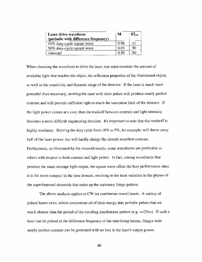
Laser drive waveform M I/Ic(periodic with difference frequency)10% duty-cycle square wave 0.98 .1150% duty-cycle square wave 0.63 .50sinusoid 0.50 .50
When choosing the waveform to drive the laser, one must consider the amount of
available light that reaches the object, the reflection properties of the illuminated object,
as well as the sensitivity and dynamic range of the detector. If the laser is much more
powerful than necessary, strobing the laser with short pulses will produce nearly perfect
contrast and still provide sufficient light to reach the saturation limit of the detector. If
the light power comes at a cost, then the tradeoff between contrast and light intensity
becomes a more difficult engineering decision. It's important to note that this tradeoff is
highly nonlinear. Halving the duty cycle from 10% to 5%, for example, will throw away
half of the laser power, but will hardly change the already excellent contrast.
Furthermore, as illustrated by the sinusoid results, some waveforms are preferable to
others with respect to both contrast and light power. In fact, among waveforms that
produce the same average light output, the square wave offers the best performance since
it is the most compact in the time domain, resulting in the least variation in the phases of
the superimposed sinusoids that make up the stationary fringe pattern.
The above analysis applies to CW (or continuous-wave) lasers. A variety of
pulsed lasers exist, which concentrate all of their energy into periodic pulses that are
much shorter than the period of the traveling interference pattern (e.g. <<25ns). If such a
laser can be pulsed at the difference frequency of the interfering beams, fringes with
nearly perfect contrast can be generated with no loss in the laser's output power.
40

3.3 An implementation of an acousto-optic projector
In the previous section we have seen how to generate a stationary interference
fringe pattern and precisely and rapidly control it's spatial phase, spatial frequency,
and intensity without a single moving elemen? using an electronic signal.
This chapter addresses some of the issues associated with implementing a
prototype of such a high-speed solid-state acousto-optic projector.
3.3.1 Target Application
Design decisions for an AFI projector depend on tradeoffs between the range and
extent of objects to be imaged, the desired resolution, and the imaging rate required.
Since our primary objective is to demonstrate the concept of a high-speed AFI projector
and to show that it can be applied to high-speed 3D imaging, a target application that
would benefit from high acquisition speed but does not require high resolution or a large
area of coverage is desirable.
One such application is 3D imaging of lip motion during speech. A 3D video of
moving lips would be useful for generating models for speech analysis, lip reading, and
voice recognition applications. Lips would also be a good target for the first prototype of
the AOM AFI projector for the following reasons:
e The resolution requirements are minimal for modeling the shape of lips. Since lips
have a smooth curved surface, resolution on the order of 1mm would be sufficient to
sample the overall shape. Resolution is in part a function of the density of fringes
3 Technically, the oscillating piezo-electric transducer inside the AOM is expanding and contracting at~100MHz. This component, however, is very robust in its frequency response.
41

projected on the object (and hence the maximum source-point separation achievable
with the AOM), and in part a function of the resolution and dynamic range of the
CCD detector. A few dozen fringes across the lips should be more than sufficient.
As will be seen shortly, this can be achieved with a variety of AOMs and can be
well resolved with many high-speed CCD cameras.
" The extent of the lips is limited and they can be imaged at close range. As a result,
projector power output of only a few milliwatts should be sufficient to illuminate the
lips a few feet away, even for very short exposure times and low sensitivity
characteristic of high frame-rate CCD cameras. Such power levels are available in a
number of inexpensive diode lasers, and are considered eye-safe even a few inches
away from the projector.
" The shape of the lips is smooth, simplifying the phase unwrapping steps in the AFI
process.
" Lips are not prone to specular reflection and can be easily coated with white powder
to improve their reflectivity properties.
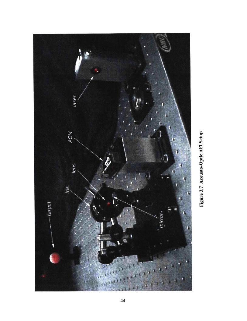
3.3.2 System design
Figure 3.6 shows a block diagram of a prototype acousto-optic AFI projector that
was built and tested in the laboratory. A photograph of the actual setup is shown in
Figure 3.7. The following subsections address design considerations for each system
component:
42

Optics
LENS
IRIS
Electronicsr------------- -----------------------------~------------~-~------~~~~~~~~~~~~|--
-I
AWG
HIGHPASSFILTERAMPLIFIER MIXER L
XTAL
Figure 3.6 Elements of laboratory acousto-optic AFI setup
43
9
0c
44

Source of coherent radiation
Choosing an illumination source involves weighing of several parameters: power,
wavelength, modulation bandwidth, coherence length, and of course cost. Since the
object proximity is on the scale of a few feet for this prototype, it turns out that a 20mW
laser would be sufficient to illuminate most objects. The common diode laser seems like
a natural choice for providing this kind of power output. Not only are diodes of this
power range commonly available, but they are much less expensive than other CW laser
technologies of comparable output power. In addition, unlike most other lasers, many
diode lasers can be modulated at rates in excess of 50 MHz -- sufficiently rapidly to be
able to generate a high-contrast stationary interference pattern -- without the need for an
external amplitude modulator. Some pulsed diode lasers are even available.
On the other hand, diode lasers typically cover longer wavelengths from red to
infrared. One would expect that a green or blue laser would produce finer fringes,
resulting in better resolution. In fact, this is not the case due to the physics of the AOM.
As the reader may recall, the angular separation between the diffracted beams, and hence
the point-source separation, is directly proportional to the optical wavelength. The spatial
frequency of interference fringes, on the other hand, is directly proportional to point-
source separation, and inversely proportional to the optical wavelength. As a result, there
is no net dependence of the fringe spacing on the optical wavelength! This can be
understood intuitively from conservation of momentum. Since photons with longer
wavelengths have less momentum than photons with shorter wavelength (momentum=
h*27/0), they are deflected by a proportionately larger angle by the oncoming sound
wave [4]. Thus, the appropriate course is to choose a wavelength near the optimum CCD
45

response. Not by accident, most CCD spectral response curves happen to coincide well
with the commonly available red and infrared diode lasers.
One disadvantage of laser diodes compared to HeNe lasers, for example, is a very
short coherence length: a few millimeters or less. Although this may not be enough in a
projector with several widely-separated optical paths, in the AOM projector both beams
share the same optical path and the coherence length required for high-contrast fringes is
simply the greatest accumulated path difference at the interference plane -- i.e. the
number of fringes in the interference pattern multiplied by the optical wavelength. For
this prototype, for example, the required coherence length is only -20gm. This is almost
achievable with some LED's!
The laser chosen for this system is a Power Technology PMT series module with
a 685nm 40mW diode laser. This very economical laser module is equipped with a TTL
trigger input, making it trivial to interface and synchronize with the RF electronics that
generate the AOM drive signal, and can be modulated at over 100MHz. While this is
sufficient to obtain stationary fringes over the entire AOM bandwidth, the -5ns step
response does not allow duty cycles below -30% with a difference frequency of 40 MHz,
for example, thereby somewhat limiting the contrast at the largest point-source
separations. A laser with an even faster modulation capability would be desirable to
obtain high-contrast interference with higher bandwidth AOM's and even greater fringe
densities.
46

Detector
Since the speed of the system is limited by the frame rate of the detector used,
choosing a high-speed CCD camera is essential. However, as the exposure time is
reduced, a stronger laser source is required to sufficiently illuminate the object. In
addition, due to the short readout time, pixel count, bit depth, well depth, and signal-to-
noise ratio of the CCD are in general sacrificed.
In this case the 8-bit 256x256 Dalsa MotionVision CA-D7 area scan CCD camera
was used with a Nikon 60mm 1:2.8D AF Micro Nikkor lens. Although this camera is
capable of rates of up to 955 frames per second, it was used at only a fraction of this
speed (90 fps) due to the available software and the capture speed of the frame grabber at
hand. As simulations have shown, the AFI technique is fairly insensitive to quantization
noise, and even four-bit signal quantization is more than enough to achieve the desired
resolution for the target application. Also, because of the low resolution requirements, a
256x256 CCD array provides a good sampling of the fringe pattern. Furthermore, even
with the lens partially stopped to increase the depth of focus, a few milliwatts of output
from the projector is enough to saturate the 11-ms exposures of the CCD because of the
proximity of the target in this case. Nevertheless, CCD speed-vs.-performance tradeoffs
must be carefully considered for more demanding applications.
47
AOM
There are many kinds of AOM's available, geared towards different applications,
different wavelengths, as well as different performance requirements. Listed below are
some important characteristics to look for when choosing an AOM for an interference
fringe projector.
* Interaction Material is the crystal material carrying the acoustic wave. Commonly
used materials are dense flint glass, PbMoO4, TeO2, germanium, and quartz. Each
material has unique optical and acoustic properties. TeO 2, for example, has the
slowest acoustic velocity (0.617mm/is) [14] and hence is used to achieve large
deflection angles and high modulation rates. Quartz, on the other hand, transmits
well in the UV range, while germanium is used mainly for far-infrared applications.
PbMoO4, which is the most commonly used material, has a relatively slow acoustic
velocity (3.63mm/gs) and is insensitive to laser polarization. Most of the AOM
models are available in several broad antireflection coating ranges.
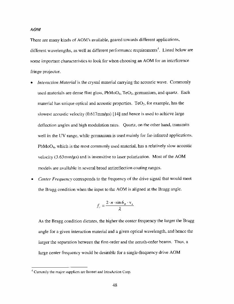
" Center Frequency corresponds to the frequency of the drive signal that would meet
the Bragg condition when the input to the AOM is aligned at the Bragg angle.
f 2n -sin 6 B -Vs
As the Bragg condition dictates, the higher the center frequency the larger the Bragg
angle for a given interaction material and a given optical wavelength, and hence the
larger the separation between the first-order and the zeroth-order beams. Thus, a
large center frequency would be desirable for a single-frequency drive AOM
4 Currently the major suppliers are Isomet and IntraAction Corp.
48
projector discussed earlier. Note that as the typical center frequencies range from
40MHz to 300MHz, it becomes increasingly challenging to synthesize and power the
AOM drive signal.
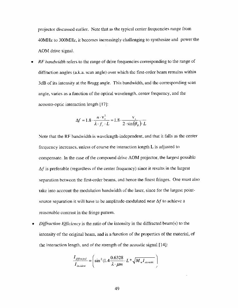
* RF bandwidth refers to the range of drive frequencies corresponding to the range of
diffraction angles (a.k.a. scan angle) over which the first-order beam remains within
3dB of its intensity at the Bragg angle. This bandwidth, and the corresponding scan
angle, varies as a function of the optical wavelength, center frequency, and the
acousto-optic interaction length [17]:
n -v 2 vAf = 1.8 - S =1.8.
2v -f.L 2 -sin(GB).L
Note that the RF bandwidth is wavelength-independent, and that it falls as the center
frequency increases, unless of course the interaction length L is adjusted to
compensate. In the case of the compound drive AOM projector, the largest possible
Af is preferable (regardless of the center frequency) since it results in the largest
separation between the first-order beams, and hence the finest fringes. One must also
take into account the modulation bandwidth of the laser, since for the largest point-
source separation it will have to be amplitude-modulated near Af to achieve a
reasonable contrast in the fringe pattern.
* Diffraction Efficiency is the ratio of the intensity in the diffracted beam(s) to the
intensity of the original beam, and is a function of the properties of the material, of
the interaction length, and of the strength of the acoustic signal [14]:
I'f'acted = sin14 0.6328 . L* MIincident w aosi
49

where Mw is a material-dependent figure of merit. Evidently, diffraction efficiency
can be increased by supplying more power to the AOM, and values above 50% can
by typically reached. While the highest possible diffraction efficiency is desired for
the compound-drive projector, a 50% diffraction efficiency would be ideal for the
single frequency drive projector that uses the first and zeroth-order beams to generate
a fringe pattern.
* Active aperture is the maximum diameter of the laser beam that will fully interact
with the traveling acoustic wave. An elliptical aperture is preferable for use with a
diode laser, since the output of most diode lasers has an elliptical crossection.
* Resolution is characterized by the number of resolvable beams (a.k.a. "spots",)5 , also
known as the rAf product, where t is the time required for the sound to cross the
diameter of the optical beam. As expected, resolution is inversely related to the well-
known divergence ratio, X/D. Thus, AOMs with larger active apertures produce more
resolvable spots and tend to be used as deflectors. Note that AOM resolution is
irrelevantfor the AFI projector. Because the laser beams have a Gaussian intensity
distribution, they expand in a hyperbolic fashion as they propagate [14], and thus do
not have to be resolved in the Rayleigh sense to generate an interference pattern. This
is illustrated in Figure 3.8. In fact, it is possible to generate almost arbitrarily large
fringes using the AOM technique simply by driving the AOM with a compound
signal with a very small difference frequency.
* Rise time is the time for the diffracted laser beam intensity to rise from 10% to 90%
of its maximum value in response to a step in the amplitude of the acoustic wave, and
5 A "resolvable spot" is defined by the Rayleigh criterion (see Hecht p371)
50

lens "source points" -- apparent origins of light- are well defined even if the Gaussianbeams are not resolved from each other
Figure 3.8 Gaussian Beam Propagation
51

determines the modulation bandwidth of the AOM. Since the entire aperture must be
filled with the new acoustic level before the diffracted beam fully responds, the rise
time is proportional to the ratio of the aperture size and the acoustic velocity. Thus,
while AOMs with a large active aperture are good beam deflectors, they are slow
beam intensity modulators. Rapid beam intensity modulation is not generally
important for an interference pattern projector. However, since rise-time is closely
related to the frequency and phase modulation bandwidth, it may be an important
consideration for interference pattern projection applications where high-bandwidth
active drift compensation is important.
* Power requirements for achieving optimum diffraction efficiency depend on the
material used, the optical wavelength, as well as on the acousto-optic interaction
length, as the diffraction efficiency equation indicates. One or two Watts of drive
power are typically sufficient for red and infra-red wavelengths. Significantly
overdriving the AOM would actually result in loss of diffraction efficiency and
eventually possible damage to piezo-electric transducer and internal power-matching
electronics.
With the above considerations as well as cost and size in mind, Isomet's 1205-C2-804
AOM coated for the operational wavelength of 685nm was used for this prototype. This
device is only 22 x 16 x 51 mm3 in size, has a center frequency of 80MHz, and has an RF
bandwidth of 40MHz, corresponding to a maximum angular separation of -0.6' between
the two first-order beams in a compound drive projector. It has a 2mm x 6mm oval
52

aperture suited for the laser diode's beam crossection, and requires - 1.5W of RF power to
achieve -85% diffraction efficiency.
RF electronics
One of the key strengths of an AOM projector is that most of the complexity is
shifted from mechanical and optical hardware to electronics. In particular, all
parameters of the fringe pattern are controlled with a single compound RF (radio-
frequency) drive signal to the AOM, which is a superposition of two sinusoids of
independently controlled frequency, phase, and amplitude.
One approach to generating such a sinusoid is to use a voltage-controlled
oscillator (VCO). Although VCOs are readily available for RF frequencies, it is rare to
find one that is linear and jitter-free over the complete bandwidth required - in this case,
from DC to 20MHz. Furthermore, in order to adjust the phase of the sinusoid, the VCO
must be placed in a phase-locked feedback loop. Such circuits are prone to phase jitter,
noise, and unwanted oscillations, and hence are difficult to design well, especially for
such a large bandwidth.
In the author's opinion, however, the simplest, most robust, and most flexible
means of generating the AOM drive signal is digital synthesis. This can be done very
inexpensively using several small Direct Digital Synthesis VLSI chips. Using a 32-bit
counter, some onboard sine and cosine ROM, and a 12-bit DAC, these chips can generate
quantized sinusoids with frequencies ranging from a fraction of a Hertz up to 40 MHz
with 32-bit precision over phase and frequency control! Alternatively, as was done in the
case of this prototype, an arbitrary waveform generator such as the Sony/Tektronix
53

AWG2010 can be used to synthesize the AOM drive waveforms. The AWG2010 also
uses DDS technology, but can be programmed to synthesize a good approximation to any
desired waveform up to approximately 50MHz in bandwidth using a 250MHz sampling
clock. A model with a 1GHz sampling clock is also currently available. Although the
AWG2010 is an expensive device, it was available for use and offers immense flexibility
for experimenting with supplying different waveforms to the AOM. By writing a simple
script on a computer and downloading it to the AWG, it was possible to generate
compound waveforms for projecting interference fringe patterns with a variety of spatial
frequencies and phase shifts. In addition, the AWG offers several TTL "marker" outputs
which are ideal for synchronously pulsing the laser at the difference frequency with a
desired duty cycle.
Because DDS produces a sampled and quantized waveform, artifacts
corresponding to harmonics of the desired frequency appear in the spectrum of the signal.
These are more problematic for low-frequency signals, since they occur closer to the
frequency of interest. The harmonics are much lower in amplitude than the main signal,
but they can be amplified by nonlinear magnitude response in the frequency multiplier
and can cause faint beams at the output of the AOM. Although this is a minor effect, it
can be removed by constructing a variable-frequency band-pass filter to isolate the
frequencies of interest and/or by carefully selecting a good RF multiplier with linear
behavior over the desired frequency and power range.
Choosing a multiplier is one of the more important decisions in the electronics
design, since it is prone to introduce or amplify noise in the signal. For this prototype,
the Mini-Circuits Level 17 ZP-3H balanced RF frequency mixer was used to multiply
54

the compound waveform by a carrier frequency. Mixers use passive components such as
diodes and inductors to multiply a weak RF signal by a stronger Local Oscillator (LO)
signal. They are inexpensive and are available for various bandwidths as well as input
power ranges. However, depending on the frequencies and power levels used, mixers can
exhibit nonlinearities including leakage of LO signal into the output, introduction of 3rd-
order harmonic distortions, and amplification of existing harmonics relative to the desired
frequency. Absolute LO power level, relative power levels of the LO and RF signals, and
the frequency of operation should be optimized against the conversion loss, isolation, and
3 rd-order intermodulation distortion curves of the particular mixer model to minimize
ghost beams such as have been seen with mixers used in the course of this work.
Alternatively, an active analog multiplier IC such as the Analog Devices AD835
can be used to multiply the signals. Unlike the mixer, which is packaged as a small box
with three SMA terminals, this chip requires some external wiring, but it offers very good
linearity and accuracy over a 200MHz bandwidth. Latest experiments are showing it to
be a big improvement over the performance of the mixers.
In order to bring the power level up to the -2 Watts required for best AOM
diffraction efficiency, the Mini-Circuits ZHL-1000-3W amplifier was used. This
amplifier can handle over 3 Watts of power, has a fixed gain of at least 38dB, and is
somewhat of an overkill for this application. Finally, a custom-made 11-pole elliptical
highpass filter was used between the amplifier and the AOM to cut off low-frequency
artifacts.
55

Optics
The optical design of this prototype consists of choosing a lens. A Nikon 4x
0. lNA microscope objective was chosen in this case to achieve a good coverage of the
object: a -100 half-angle measured along the major axis of the elliptical light cone.
Because microscope objectives are designed to have a distant back-focal plane, they are
ideal for focusing a coherent laser beam. On the other hand, an AR-coated plano-convex
lens with a 10mm focal length would probably have worked just as well, and possibly
better since the microscope objective was not coated specifically for 685 nm.
Note that there is an important tradeoff between fringe density and beam
divergence to consider when choosing the focal length of the lens. The source point
separation due to a given difference frequency in the AOM drive signal, and hence the
resulting fringe density, is a function of the focal length of the lens. For a thin lens, this
dependence can be approximated as:
a ~ f -tan(A)~ f -A.Afn-vS
where f is the focal length of the lens, and a is the point source separation, and AO is the
angular separation between the interfering beams. Although increasing the focal length
results in a larger a and a finer fringe spacing, it also reduces the divergence of the
interfering beams. In fact, the total number of visible fringes is always the same.
As shown in the diagram, an iris was placed at the focal plane to block the zeroth-
order beam from interfering with the first-order beams. A more comprehensive solution
would be to make a spatial filter mask by placing a thin metal plate at the focal plane and
drilling minute apertures at locations corresponding to the desired source-point
56

separations. In addition to blocking the zeroth-order beam as well as any ghost beams
generated by harmonics in the AOM drive signal, it would also serve to remove most
distortions present in each beam and the associated background noise in the interference
pattern by filtering out everything except the central Gaussian lobe in the beam's focal
plane diffraction pattern.
3.3.3 Results
The complete system is capable of projecting over twenty interference fringes
with a 40MHz difference frequency driving the AOM. This is more than sufficient to
demonstrate the concept of a solid-state projector and to be able to create surface maps of
some interesting objects.
Figure 3.9 shows a golf ball illuminated by interference fringes produced with the
acousto-optic projector. In this case 30MHz difference frequency was used to drive the
AOM, and a 25% duty cycle square wave was used to pulse the laser. The fringes exhibit
good contrast, as would be expected from a 90% modulation depth predicted by
simulations.
The golf ball was coated with white spray paint to eliminate specular reflections
from some patches of the glossy surface. Depending on the chosen exposure time, such
anomalies lead to either saturation of the CCD in those areas, or to reduced sensitivity in
the areas that do not produce specular reflection. This kind of abrupt intensity variation
will be true of many potential targets with varying textures and surface angles. While
coating the object with diffuse paint can be an effective approach, paint not only hides the
finer features on the object's surface, but usually destroys the object -- an outcome that is
57

00
Figure 3.9 Results: 30MHz fringes on a spray-painted golf ball

often not desirable. Another way of using the CCD's dynamic range efficiently for all
regions of the object without coating it is to take a succession of exposures at different
interference fringe intensities. By using the dimmer fringes to reconstruct the bright
surface patches and using the brighter fringes to reconstruct the more diffuse areas, the
complete surface map can be obtained 6. For stationary objects, the high frame rate of an
AOM-based AFI system allows taking a rapid progression of exposures at a wide range
of fringe intensities, enabling the reconstruction of all illuminated surfaces for a generic
object with unknown surface reflectance properties.
Also visible in Figure 3.9 is slight background intensity structure in the
interference pattern due to intensity variations in the laser beam (dirt on the optics would
produce much more conspicuous circular diffraction patterns). Although one of the
benefits of the AFI technique is that phase measurements are minimally affected by such
spatial intensity variations in the laser beam, these local brightness variations do act to
slightly reduce the dynamic range available in some areas of the object. A more
pronounced setback is dealt to the visual appeal of the interference pattern. As
mentioned before, however, placing a spatial filter mask at the focal plane of the focusing
lens can among other things greatly improve the appearance of the fringes.
Although the AOM used in this experiment is capable of projecting only about
two dozen fringes, fringe density can be greatly increased for more demanding
applications by using an AOM with a greater RF bandwidth, or by interfering the first-
order diffracted beam with the zeroth-order beam and using a single frequency to
generate the acoustic wave. Used in this fashion, the Isomet LS55 AOM, for example,
6 The saturated pixels may "bleed" into neighboring pixels, reducing the effectiveness of this approach nearsaturated regions. Many CCD's, however, have anti-blooming gates that greatly reduce this effect.
59

can produce nearly 400 fringes -- far more than can be taken advantage of by most
scientific CCD cameras. Even higher angles of deflection can be obtained through "beam
steering" [17]. This technique relies on a serially-stacked phased array of piezo-electric
transducers along the acousto-optic crystal to "steer" the beam further and further from
the Bragg angle. Although more costly to implement, this approach can potentially be
used to generate thousands of fringes.
3.4 Benefits of the acousto-optic projector
The acousto-optic projector has few inherent limitations. Even though the
number of projected fringes is limited by the deflection range of the AOM, hundreds or
thousands of fringes can be generated if necessary using the beam steering approach
mentioned above. Another issue is the loss of laser power due to amplitude modulation
of the laser beam necessary to freeze the traveling fringes. However, even with 50%
modulation, high contrast fringes can be obtained7 . On the other hand, the acousto-optic
projector has many benefits to offer for projecting interference patterns in general and for
Accordion Fringe Interferometry in particular:
e Robustness: The acousto-optic projector consists of only four elements: a laser, an
AOM, a lens, and RF electronics. It is not difficult to fathom the ruggedness and
reliability of the solid-state optical and electronic components. The AOM itself is
also very robust. Acousto-Optic Modulators are used for modulating laser intensity,
scanning laser beams, and frequency filtering in a variety of applications and can
7 It may be possible to generate and control stationary fringes without the need to modulate the laser beamby inducing standing waves in the acousto-optic crystal. This approach is yet to be explored.
60
handle a range of optical powers up to 200W. High quality laser printers, optical
signal processing, spectroscopy, and rangefinding are just some of the industrial and
military applications that rely on AOMs. As a result, AOMs are made to be very
dependable and suitable for use in adverse environments. By contrast, high vibration,
temperature drifts, and large gravitational forces would pose insurmountable
obstacles for a projector system that relies on moving components.
Accuracy and Repeatability: Given a stable environment, the resolution in the spatial
phase and frequency of the projected interference pattern is dependent largely on the
precision of the electronics and the optical quality of the collimating and focusing
lenses. With a 32-bit resolution in the frequency and phase of the digitally-
synthesized electronic signal, frequency steps of a few millihertz, and phase shifts of
a few nanodegrees can be made repeatedly! This kind of performance can not be
matched by a system that relies on moving components, where frequency and phase
uncertainties are a significant source of error in data processing. Of course,
temperature drifts can result in mode-hopping of the laser, as well as distortions in the
optical path of the laser beam. This kind of behavior, however, will affect any
optical system that relies on a laser, and well known environment control techniques
can be used to mitigate the effects. In addition, due to the fast, complete, and precise
control over the fringe pattern, active compensation for temperature drift may be
effective with the acousto-optic projector.
* Speed: Modulation bandwidth of nearly 1MHz is more than is required for updating
the fringe pattern at video rates. This large of response rate, however, can be utilized
in a high-speed electronic feedback system interfacing the AOM drive electronics
61

with a series of sensors (e.g. accelerometers, photodetectors, temperature sensors) to
allow active compensation for high-frequency vibrations and temperature fluctuations
in the environment. In addition, the high modulation rate can be used to measure
high-frequency vibrations in three dimensions - by matching the phase or frequency
of the fringes with a lateral or range motion of a vibrating reference pattern, for
example.
" Arbitrarily large reference fringes: Because of the very small source-point
separation involved (e.g. 4gm), projecting large stable interference fringes can be a
source of difficulty for an interference projector that relies on rearrangement of
optical components to control fringe density. For a compound-drive AOM fringe
projector, on the other hand, the spatial frequency of the fringe pattern is a function of
the difference frequency in the AOM drive signal only, and as a result can be made
almost arbitrarily small. Although the present AFI technique does not need to rely on
large interference fringes for phase unwrapping, the capability of generating them
offers another degree of flexibility in projecting an interference pattern in general.
* Short coherence length: Due to the shared optical path of the two interfering beams
in the acousto-optic projector, the coherence length requirements are very relaxed -
e.g. on the order of 20gm - allowing for a greater choice in sources of illumination.
" Portability: With a diode laser as the radiation source, at 22x16x51 mm3, the AOM
is the largest component in the optical path of the acousto-optic projector, fitting
comfortably on the palm of a hand. AOM drive electronics using DDS VLSI
technology and a custom-made amplifier can be made small enough for the entire
device to occupy a volume the size of a person's fist (batteries not included).
62

* Economy: If a DDS VLSI strategy for the RF electronics is pursued, the cost of such
a system today would be somewhat evenly distributed between the AOM, the diode
laser, and the entire package of electronics, amounting to an estimated parts cost of
$2000 for a single prototype, although for an application demanding more fringes, a
more expensive AOM would be in order. Of course, the projector can be mass-
produced at a fraction of this cost, resulting together with an economical CCD
detector in a 3D imaging product affordable to the research community, and
ultimately to the consumer.
63

Chapter 4
Depth-Retrieval For Stationary and Moving Targets
Although the main objective of this work was to design and implement a high-
speed interference pattern projector, a basic algorithm for automatically extracting depth
information via spatial phase estimation was also implemented in order to demonstrate
the 3D imaging speed possible with an acousto-optic AFI system. The algorithm as well
as the 3D reconstructions obtained with a prototype acousto-optic AFI system are
discussed below.
4.1. Algorithm for depth retrieval using spatial phase estimation
4.1.1 Triangulation
As explained in Chapter 2, depth information about a reflective object can be
obtained by projecting an interference fringe pattern onto the object followed by
triangulation using a single detector. The triangulation model used for this algorithm is
64
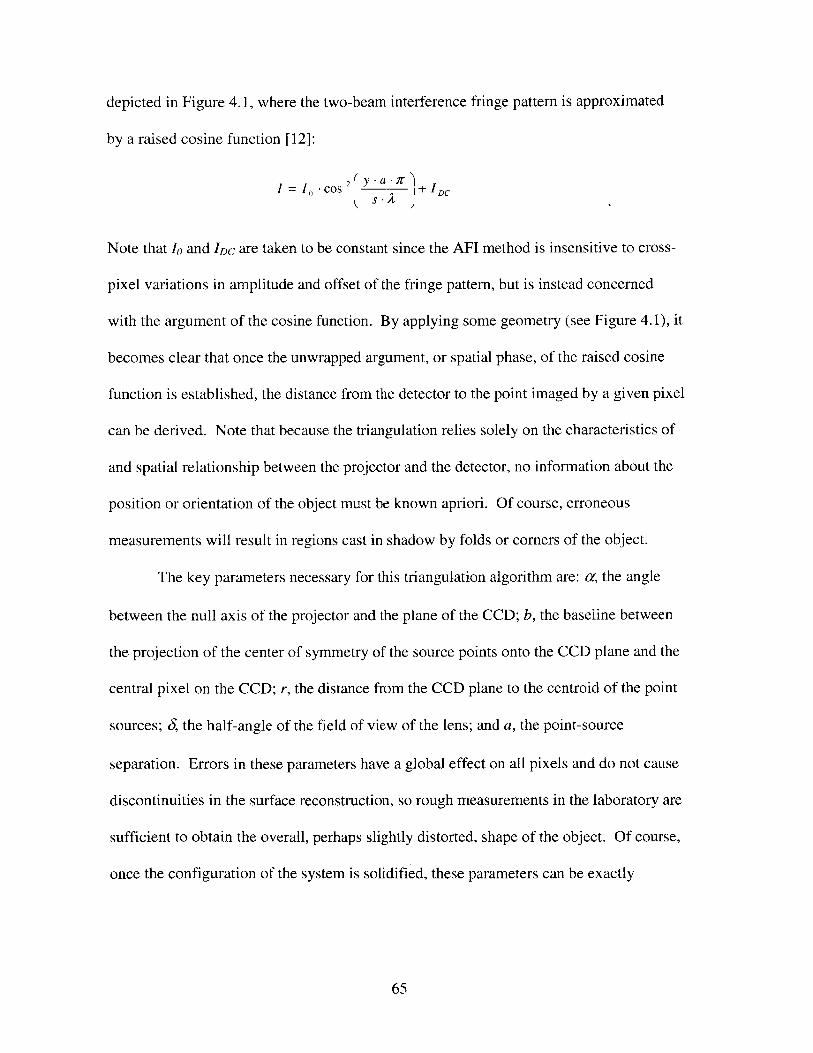
depicted in Figure 4.1, where the two-beam interference fringe pattern is approximated
by a raised cosine function [12]:
S= Io.Cos 2 Y -a -1+ I DC
Note that Io and IDC are taken to be constant since the AFI method is insensitive to cross-
pixel variations in amplitude and offset of the fringe pattern, but is instead concerned
with the argument of the cosine function. By applying some geometry (see Figure 4.1), it
becomes clear that once the unwrapped argument, or spatial phase, of the raised cosine
function is established, the distance from the detector to the point imaged by a given pixel
can be derived. Note that because the triangulation relies solely on the characteristics of
and spatial relationship between the projector and the detector, no information about the
position or orientation of the object must be known apriori. Of course, erroneous
measurements will result in regions cast in shadow by folds or corners of the object.
The key parameters necessary for this triangulation algorithm are: a, the angle
between the null axis of the projector and the plane of the CCD; b, the baseline between
the projection of the center of symmetry of the source points onto the CCD plane and the
central pixel on the CCD; r, the distance from the CCD plane to the centroid of the point
sources; 6, the half-angle of the field of view of the lens; and a, the point-source
separation. Errors in these parameters have a global effect on all pixels and do not cause
discontinuities in the surface reconstruction, so rough measurements in the laboratory are
sufficient to obtain the overall, perhaps slightly distorted, shape of the object. Of course,
once the configuration of the system is solidified, these parameters can be exactly
65

null line
b(baseline)
I =IO -COS2.Ya II+IDC
(z - y cosa+ r)
sina
= I0 Cos 2(Ounwrapped )+ 'DC
y y sin a - $Aunwrapped -tanss z+r-ycos a a-7c
x=z.tan#8 -- y=[z+r-(b-x)-tana-cosa=z.(tan#.sina+cosa)-b-sina+r-cosa
rtan 6 +(b sin a -rcos a). (tan 6 -cos a +sin a)
(tan # -sin a + cos a). (tan 9 -cos a + sin a)- tan 6
Figure 4.1 Triangulation
66
a

measured, and absolute depth measurements can be obtained for any object placed in the
field of projected illumination.
4.1.2 Phase Unwrapping
Errors in the phase-map, on the other hand, will vary from pixel to pixel, causing noise
and discontinuities in the reconstructed surface of the object. Thus it is the process of
measuring and unwrapping the spatial phase for each pixel that is the main challenge in
an AFI algorithm. The implemented phase unwrapping method is based on the
Progressive Fringe Division algorithm developed by Shirley [1]. It relies on phase
measurements taken at a progression of fringe spacings to unwrap the phase measurement
taken at the smallest fringe spacing independently for each pixel. As explained in
Chapter 2, at each point-source separation a in this progression, the phase at each pixel is
computed to within a 360' ambiguity by imaging three fringe patterns phase-shifted
relative to each other by 90'. Note that no matter what a is, the spatial coordinate of the
pixel (triangulated from tan0) must remain the same. Therefore, we can unwrap a phase
measurement taken at a given point source separation a, by finding that integer fringe
number n that results in a value of (tanG )1 that is nearest to (tan9)2 calculated using an
unwrapped reference phase measurement taken at a smaller point source separation a2.
The entire process is illustrated in Figure 4.2 from the point of view of a single pixel and
the pixel array as a whole.
The software written to implement this algorithm consists of several self-
documenting Matlab modules, which are included in Appendix A. The surface
reconstruction algorithm was tested for correctness using simulations in Matlab. A
67

initialy, project a single referencefringe, so that no unwrapping isnecessary
/012 (900)
11 (90*)unwrapped phase
12 (0*) #=tan 2I2Y (I + I3)_
13 (+900) wrapped phase
phase-shiftedreference fringe
fringe numbers n
tan 0, ~=tn 2-+> n = round - 0 #2 -) 011
# 2 = ( tan B 2 x ' 2 4_2 T
11 (-90*)unwrapped phase
42 12 (00)
13 (+900)
phase-shifted fri
wrapped phase
igesthis unwrapped phase-map isused as a reference tounwrap even finer fringes
Figure 4.2 Phase unwrapping
68
surface was generated using the peaks function, and simulated fringe patterns of different
densities were projected onto it using the raised-cosine model (without taking shadows
into account). The algorithm outlined above was then used to reconstruct the 3D surface.
As shown in Figure 4.3, the reconstructed surface is indistinguishable from the original
peaks function. The same results were obtained with a variety of geometric system
parameters used to simulate the fringes. The Matlab functions and scripts used to
perform the simulations are also included in Appendix A.
4.2 Measurements and Results
To test the acousto-optic AFI system as a whole, a white spray-painted golf ball
was used as a target. The golf ball was placed 56cm away from the focal plane of the
projector, and the geometric parameters necessary for triangulation were measured to be:
a=43', b =370mm, r =-426mm, and i=1.72'. Three fringe spacings used to unwrap the
phase were generated using difference frequencies of 1,6, and 40MHz in the AOM drive
signal, corresponding to source-point separations of 4.45, 26.7, and 178gm, respectively.
A 50% duty cycle square wave was used to drive the laser in all three cases, resulting in a
66% modulation depth of the fringes. Figure 4.4 shows the three resulting fringe
patterns, the corresponding wrapped phase-maps calculated using three 90' phase-shifts
at each fringe separation, as well as the unwrapped phase-maps produced using the
algorithm outlined above. All nine exposures were taken in 100 milliseconds with the
256x256 8-bit Dalsa CA-D7 CCD camera running at 90 frames per second.
The resulting surface map shown in Figure 4.5 demonstrates the feasibility of
autonomous high-speed 3D imaging with an acousto-optic AFI system. In addition to the
69

distance from source: 50cmdepth extent: 5 cm
Simulated Surface
50 100 150 200 250
Simulated fringe projection
300
Reconstructed Surface
Figure 4.3 Simulations show algorithm correctness
70

50
100-
150-
200-
250
50 100 150 200
2 MHz differencefrequency fringes
250
+
50 100 150 200
6 MHz differencefrequency fringes
+
250
40 MHz differencefrequency fringes
+
100
150
200
250 250 250
50 100 150 200 250
40 ~zwrape
2 MHz wrappedphasemap
2 MHz unwrappedphasemap
6 MHz wrappedphasemap
6 MHz unwrappedphasemap
40 MHz wrappedphasemap
40 MHz unwrappedphasemap
Figure 4.4 From Fringes To Phasemaps
71
50.
100
150 -
200.
250
50
100
150
200
250
50 100 150 200 250, , ,
OU IUU IOU ZW

500
300
250
300250
200
100150
50
80 100 120 140 160 180 200 220 240
Figure 4.5 3D reconstruction of the illuminated surface of a golf ball
72

short data acquisition time, it took only -4 seconds on a 166 MHz Pentium-class
computer to reconstruct a surface from the collected data -- without significant
optimizations in the Matlab code. This processing time is encouraging, since it suggests
the possibility of real-time processing using a dedicated DSP board.
This first attempt at a 3D surface reconstruction using acousto-optic AFI not only
shows the overall shape of the golf-ball, but also resolves sub-millimeter indentations in
the golf ball. The errors in the surface map also reveal some issues to be considered
when making 3D measurements using this system in the future.
For example, it is evident from the images in Figure 4.4 that the intensity of the
reflected light is distributed very unevenly across the golf ball due to the varying
orientation of the surface. While there is little that can be done about this for a quickly
moving target, for a stationary object a series of nine-frame sequences of varying
intensity could be taken to cover the entire surface of the golf ball with fringes as outlined
in Chapter 3.
One may also notice that the fine background fringes are better focused than the
larger foreground fringes. Badly focused fringes tend to smear phase measurements of
neighboring pixels, ultimately resulting in a loss of depth resolution. If there is no
shortage of light, a greater depth extent of the object can be brought into focus by
increasing the laser intensity and stopping down the lens aperture to increase the depth of
focus of the detector.
Also, evident in the surface reconstruction, are small-amplitude high-frequency
ridges that are present throughout the surface and appear to trace the curvatures of the
8 The size of imaged laser speckle tends to increase as the lens aperture is reduced. Since laser speckle is asource of noise in phase measurement, this tradeoff must also be considered.
73

interference fringes. The most likely cause of these irregularities is the presence of
"ghost" beams due to harmonics in the electronic AOM drive signal. Since the phase of
the faint low contrast fringes produced by the ghost beams correlates with the phase of
the primary fringes, the ghost fringes would not be eliminated with the background and
would introduce regular errors in the spatial phase estimation. These ghost beams have
been observed at the output of the AOM when an RF mixer was used to multiply the
drive frequencies, as was the case for this measurement. Recent tests indicate that the
AD835 active multiplier produces a much cleaner drive signal, and will likely replace the
mixer in the next implementation of the acousto-optic projector.
Perhaps most striking, however, is the presence of "canyons" on the reconstructed
surface. Unlike the noise present in the shadowed regions, these features are clearly not
due to large random errors in phase measurement, but are due to errors in phase
unwrapping. Examination of the unwrapped phase-maps reveals that while the 6MHz
phase-map is unwrapped correctly resulting in a smooth phase variation, the 40MHz
phase-map exhibits jumps in phase corresponding to the locations of the canyons. This
leads one to conclude that the phase resolution in the suspect areas of the 6MHz phase-
map is not good enough to disambiguate 360' jumps in the 40MHz phase-map. As
explained in Chapter 2, it is this kind of behavior that ultimately determines how many
sets of reference fringes are needed to unwrap a high-resolution phase-map, and what
frequency ratios should be used. In this case, changing the difference frequency for the
second reference phase-map from 6MHz to 8MHz, for example, may result in a better
unwrapping. The signal-to-noise ratio, and hence phase resolution, can also be improved
by increasing the contrast of the fringes by pulsing the laser with a shorter duty cycle
74

square wave and by increasing the available dynamic range in the manner described
above.
It may not be even necessary, however, to unwrap the 40MHz phase-map. For
many 3D applications resolving sub-millimeter indentations on an object is not required,
but a representation of the overall shape of the object is desired instead. For such
applications, imaging fringes produced with 1MHz and 6MHz difference frequencies, for
example, would be sufficient to determine the overall shape of the golf ball, and would
result in 33% increase in data acquisition rate. Figure 4.6 shows a 3D reconstruction of a
LEGOTM knob made with 2MHz and 10MHz difference frequencies, and thus six frames
in total. If one's goal is resolve the letters on the stud, clearly 10MHz fringes provide
sufficient resolution.
75

Figure 4.6 Reconstruction of a LEGO stub using only six CCD frames
76

Chapter 5
Conclusions
The previous chapters have discussed and demonstrated how acousto-optics can
be used in an Accordion Fringe Interferometry system to acquire the data necessary to
reconstruct the 3D surface of an object at video-rates and faster. Listed below are some
ideas for future projects that can help transform acousto-optic AFI from a proof of
concept into a useful and novel 3D imaging system.
Making acousto-optic AF portable and inexpensive:
The optics of an acousto-optic AFI system consist of a diode laser, a crystal, a
lens, and a CCD camera. It is easy to envision all of these solid-state components
miniaturized and fitted into a pill box, or even printed onto a machine-vision circuit
board.
Ironically, the largest and most expensive components of the implemented AFI
system are the RF electronics. However, an expensive arbitrary waveform generator,
which was used for maximum flexibility in the laboratory, is not necessary to control the
phase and frequency of the fringe pattern for the purposes of AFI. In fact, it can be
77

replaced without sacrifice with a VLSI Direct Digital Synthesis integrated circuit, such as
the Qualcomm Q2368 (which is currently priced at about $16). The Q2368 can
synthesize a single sinusoid with a 130MHz sampling clock, or two independently-
controlled sinusoids using a 65MHz sampling clock, and uses 32 bits to encode both
frequency and phase of the synthesized waveform. A high-speed DAC is needed to
convert its 12-bit output into an analog waveform. A design of AOM control electronics
using the Q2368 chip is shown in Figure 5.1. Furthermore, a compact 1.5 Watt RF
amplifier can be designed [18] to amplify the RF output of the DDS system to the levels
necessary to drive the AOM.
Making a video-rate acousto-optic AFI system:
The speed of an acousto-optic AFI system is limited by the frame rate of the
detector, since the projector can update the fringe pattern close to a million times per
second. Although the implemented system is already capable of reconstructing nearly
100 surface maps per second by running a 256x256 CCD camera at almost 1000 fps, it is
desirable to be able to achieve high 3D reconstruction rates with less exotic cameras.
Two parallel roads can be pursued towards achieving this goal: minimizing the number of
frames necessary to reconstruct the surface of an object to reduce the latency of the
system, and studying the effects of pipelining CCD frames to increase the throughput.
Statistical analysis [19], can be used to rigorously optimize the sampling of the fringe
space.
78

AOM
t80 MHz
s i n e
F
XTAL RFAMP
MULT-- " 0 C K(AD>835
LhOCKIVIDER
.. LS163)
DAC LPF
~ 100-bHz - E-(AD9760) 30Mliz
Q2368 5DDS
(dual mode)DA C LPFI10-bit
100 MHz t(AD9760) 30MHz
A LASERDIODE
DRIVER(AD9660)
LASER
Figure 5.1 RF drive electronics using Qualcomm Q2368 DDS integrated circuit
79

Although fast 3D acquisition is clearly possible with a fast enough detector,
applications such as machine vision, or quality control on a fast conveyor belt may
require real-time processing of the data as well. While the -4s processing time required
to reconstruct a surface in Matlab on a 133MHz Pentium machine is very encouraging,
the performance possible with dedicated DSP-based hardware9 is not yet clear. Because
of the pixel-independent nature of the AFI technique, parallel processing approaches may
improve processing time tremendously.
Taking advantage of the AOM's modulation bandwidth:
While the image acquisition rate of the AFI system is limited by the frame rate of
the detector, one can still take advantage of the high update speed of the acousto-optic
projector. By interfacing the AOM with a variety of sensors via a high-speed feedback
system, for example, it may be possible to actively compensate for the effects of vibration
or high-frequency turbulence in the atmosphere, which are detrimental not just for high-
speed AFI, but for a number of interferometry techniques that rely on projecting
interference fringe patternso
Designing a sensory aid fJr the blind:
A particularly inspiring and helpful application for a high speed 3D imaging
system is a novel sensory aid for the blind. A portable device comprised of a video-rate
AFI system interfaced with a high-bandwidth tactile display, may allow a blind person to
navigate and recognize remote objects by feeling a rapidly-updated 3D model of the
9 A programmable DSP board geared for video-rate processing for machine vision applications is availablefrom Digital Designs of Cambridge, MA.
80

environment with his or her fingertips. Such an acousto-optic AFI system can illuminate
and image the volume of a small room from several meters away using a 100mW IR
laser, for example, offering a significant extension to the range and the bandwidth of a
Iwalking cane".
This thesis has demonstrated that a solid-state acousto-optic interference fringe
projector is a practical device and can be interfaced with a high-speed imager in a 3D
measurement system that is fast, robust, accurate, repeatable, portable, and economical.
It is the author's hope that this work will help bring Accordion Fringe Interferometry into
the world of entertainment, medicine, and research and help advance our ability to
exchange 3D information in the course of our everyday lives.
81
'0 See for example proposal for active control of antenna surfaces [20]" Professor Kenneth Salisbury of the Artificial Intelligence laboratory at MIT is currently conductingresearch in the field of tactile interfaces.

Appendix A: An Implementation of the AFI Algorithm
% this scripts places a surface in sumulated space using the peaks function,% projects two sets of fringes onto it (large reference fringes, and fine fringes),% reconstructs the surface using phase measurement and triangulation,% and plots the surface
% the siumulated fringes are quantized using 256 levels% no noise is added to the fringes in this case% shadows are not simulated
% the geometric parameters are as follows:
% distance of object center from CCD: 50cm% maximum range extent of object: 5cm
% lambda=685 nn% alpha=pi/4.2% r=-476 im% b=370 nOm% delta=pi/104
% point source separations used:% reference: a=0.0005 mm% fine: a=. 178 mm
LO=clock;hmap=peaks(256);hmap=stretch(hmiap,256);hmap=putheader(hmap, 'lambda',0.G00685,'a',.178, 'alpha',pi/4.2, 'r',-426,'b',370,'delta',pi/104);frl=fringepainthrmap,-pi/ 4
,0.195,792,256,0,0);fr2=fringepaint(hmap,0,0.195,792,256,0,0);fr3=fringepaint(hmrap,pi/4,0.195,792,256,0,0);pmap=phasemap(frl,fr2,fr3);hmap=(putheader(hmap,'a',0.0005));friref=fringepaint(hmap,-pi/4,0.195,792,256,0,0);fr2ref=fringepaint(hmap,0,0.195,792,256,0,0);fr3ref=fringepaint(hmap,pi/4,0.195,792,256,0,0);pmapref=phasemap(frlref,fr2ref,fr3ref);n=p2n(pmap,pmapref,copyheader(zeros (256) ,pmapref));z=p2z(pmap, n);surfl(stretch(z(2:end, :),256) );shading interp; colormap grayetime(clock,tO)
function fringes=fringepaint(hmap,phase,zscale,zdist,signal,bkg,noise);% fringepaint(hmap,zscale,zdist,signal,bkg,noise);% maps a 2-d image, hmap, into xyz-space based on the level (hmap must have a header)% paints the xyz-space with fringes to simulate data
% - phase of the cos^2 fringe function (note, 900 shift in cos = 450 shift in cos"2)% - zscale is in mm/(hmap unit)% the higher the hmap, the closer to camera% - zdist is the distance from the CCD to the surface at center of f.o.v. (mm)% - signal is the number of levels of the projected fringe pattern% - bkg is the number of levels of the noise floor% - noise is the MAGNITUDE of the maximum random noise level
% to see header variables, type "help headertable"
lambda=getheader(hmap, 'lambda');a=getheader(hmap, 'a');alpha=getheader(hmap, 'alpha');r=getheader(hmap, 'r');b=getheader(hmap, 'b');delta=getheader(hmap, 'delta');
82
fringes=hmap;% remove headerhmap=hmapa(2:end,:);
len=size(hmap,2);height=size(hmap,l);midpointx=round(len/2);midpointy=round(height/2);z=zdist+zscale." (hmap(midpointy,midpointx) -hmap);indexesx=[1:len];indexesy=[1:height];[x dummy] =meshgrid (indexesx, indexesy);clear dummy;
% do reverse-triangulationtanbeta=tan( (x-midpointx) /midpointx*delta);x=z.*tanbeta;y=(z+r-(b-x)*tan(alpha))*cos(alpha);s=(z+r-y*cos(alplia))/sin(alpha);
% generate additive phase noisenz=0;if (noise - 0)
nz=floor((0.5 -rand(height,len))*2*noise);end;
% implement TI=IOcos^2 (ya*pi/ (s*lambda)frinqes(2:end, :)=floor ((signal-1) *(cos(a*pi/lambda*y./s+phase)) .2)+nz-floor(bkg)
function p=phasemap(Il,I2,I3);% phasemap(Il,I2,I3);% calculates phase based on three measurements of the fringe sinusiod 900 apart% note: order of phasemaps is important: Tl=--90 0
, I2=00, I3=900
% to see header variables, type "help headertable"
% copy headerp=Il;
%strip headersI1=Il(2:end,:);12=I2(2:end,:);13=I3(2:end,:);
p (2:end, : )=atan2 ((Il-13), (2*I2-11-13) )./2;
function n=p2n(p,pref,nref);% p2n(p,pref,nref);% calculates a fringe-number n for each pixel based on reference phase-map% fringe numbers are used to unwrap the phasemap later%% to see header variables, cype "help headertable"
%copy headern=p;
a=getheader(p,'a');
if (getheader(pref, 'id') ~= getheader(nref, 'id'))warning('Pref and Nref have different session IDs')
endif (getheader(pref, 'a) - getheader(nref, 'a'))
warning('Pref and Nref have different source separations')end
aref-getheader(pref, 'a');
%strip headersp=p(2:end,:);pref=pref(2:end,:);nref=nref(2:end,:);
n(2:end, :)=round ((a/aref* (pref+nref*pi)-p)./pi);
83

function z=p2z(p,n);% p2z(p,n);% calculates depth map from the wrapped phasemap and fringe numbers% (see Figure 4.1 in text for derivation of triangulatin formulas)
% to see header variables, type "help headertable"
lambda=getheader(p,'lambda');a=getheader(p,'a');alpha=getheader(p,'alpha');r=getheader(p,'r');b=getheader(p,'b');delta=getheader(p,'delta');
if (getheader(p,'id') - getheader(n,'id'))warning('P and N have different session IDs');
end
if (getheader(p,'a') ~ getheader(n,'a'))warning)'P and N have different source separations');
end
sina=sin(alpha);cosa=cos(alpha);
z=p;
%strip headersp=p(2:end,:);n=n(2:end,:);
tantheta=(p+n*pi)-lambda/(a*pgi);len=sizep,2);midpointx=round(len/2);
xpix=p;for i=l:len
xpix(:,i)=- midpointx;end;
tanbeta=tan(xpix/(midpointx/delta));
z(2:end,:)=(r.*tantheta+(b*sina-r*cosa) .* (tantheta.*cosa+sina) ) ./((tanbeta. sina+cosa) *(tantheta.*cosa+sina)-tantheta);
function names=headertabie();% headertable();% returns a cell array of variable names, in the order as they appear in header
% THE HEADER FOLLOWS THE FOLLOWING FORMAT:% header is the first row of matrix, and is as follows:% columns in increasing order:% 1-6: tag ='header' (used to distinguish matrixes with headers from raw matrixes)% 7: ID =-this is the non-zero ID of the session% 8: lambda =laser wavelength (min)% 9: a =source separation (rm)% 10: alpha =angle between source and detector normals (rad)% 11: r =distance from CCD plane to source midpoint (away from object) (min)% 12: b =baseline between the ccd center and the source midpoint projection ontoccd plane (mm)% 13: delta =halfangle f.o.v. of lens (rad)
names={'id' 'lambda' 'a' 'alpha' 'r' 'b' 'delta'};
f unction value=getheader(mat,name)% getheader(mat,name)% returns the value of the desired header variable
% to see header variables, type "help headertable"
names=headertable;tag=double('header');
if (mat(1,1:6) - tag)error('This matrix does not have a header. Aborting.')
84
end;
found=0;
for j=l:iength(names)if (strcmp(name,names(j)))
value=mat(1, (length(tag)+j);found=;-
end;end;if (found == 0)
sprintf('!!!Warning!!! variable "%s" not found in header',name)end;
function mat=putheader (mat, varargin);% putheader(mat,varargin);% assigns a value to the desired header variable(s)% varargin format: 'name',value, 'name',value, etc...%
% to see header variables, type "help headertable"
if (mod(length(varargin),2) ~ 0)error('Incorrect number of arguments. Aborting.')
end;
names=headertable;tag=double('header');
% if mat has no header, create oneif (mat(l,1:6) - tag)
tempmat=mat;matzeros(size(mat,1)+1,size(mat,2));mat(l,1:6)=tag;mat (2: end, : ) =tempmat;clear tempmat;
end;
found=0;
for i=1:2:length(varargin)for j=l:length(names)
if (strcmp(varargin{i),names(j)))mat(1, (length(tag) +j))=varargin{i+l};found=1;
end;end;if (found == 0)
sprintf('!!!Warning!!! variable "%s" not found in header',varargin{i})end;
end;
function host.copyheader.(host,.donor)% hosth-copyheader~host,donor);% copies the header from the donor to the host% host does not have to have a header
% to see header variables, type "help headertable"
tag=double('header');
if (donor(1,1:6) - tag)error('Donor does not have a header. Aborting.')
end;
% if host has no header, create oneif (host(1,1:6) -= tag)
temphost=host;host=zeros(size(host,1) +1,size(host,2)host(l,:)=donor(1,:);host(2:end,:)=temphost;clear temphost;
% otherwise, just copy headerelse
host(l,:)=donor(l1,:);end;
85
Bibliography
[1] L.G. Shirley, "Three-Dimensional Imaging using Accordion Fringe Interferometry",
to be published, Applied Optics
[2] L.G.Shirley, "Accordion Fringe Interferornetry: A Novel 3D Imaging Technique",
MIT Lincoln Laboratory Staff Seminar, 31 January 1997.
[3] Sumit Basu, "A Three-Dimensional Model of Human Lip Motion", Master's Thesis,
Massachussets Institute Of Technology, Department of Electrical Engineering and
Computer Science, 1997.
[4] Joseph Karlin, "3D Imaiging methods for manufacturing, with Emphasis on the Laser
Speckle Technique", Master's Thesis, Massachussets Institute Of Technology,
Department of Mechanical Engineering, 1995.
[5] D. Nitzan, "Three-Dimensional vision structure for robot applications". IEEE
Transactions on Pattern Analysis and Machine Intelligence, Vol. 10, No.3, May
1988.
[6] D. Svetkoff, "Towards a High Resolution, Video Rate, 3D Sensor for Machine
Vision", SPIE, vol 728, 1986.
[7] Paul J. Besl, "Active, Optical Range Imaging Sensors", in Saanz, Jorge L.C., ed.,
Advances in Machine Vision, Springer-Verlag, New York, Chapter 1, 1989, pp 1-6 3 .
86

[8] Lyle G. Shirley, Emory D. Ariel, Gregory R.Hallerman, Harold C. Payson, and John
R. Vivilecchia, "Advanced techniques for target Discrimination Using Laser
Speckle", MIT Lincoln Laboratory Journal, Vol. 5, No. 3, Fall 1992.
[9] Lyle G. Shirley, Gregory R.Hallerman."Applications of tunable Lasers to Laser Radar
and 3D Imaging", MIT Lincoln Laboratory Technical Report No. 1025, 26 february
1996
[10] John M. Fini, "Three Dimensional Image Reconstruction from Fourier Magnitude
Measurements", Master's Thesis, Massachussets Institute Of Technology,
Department of Electrical Engineering and Computer Science, 1997.
[11] Michael S. Mermelstein, "A Large-Scale Three-Dimensional Imaging System Based
On Laser Speckle", Master's Thesis, Massachussets Institute Of Technology,
Department of Electrical Engineering and Computer Science, 1995.
[12] Eugene Hecht, Optics , 2 "d Edition, Addison-Welseley Publishing Co., © 1987
[13] Brillouin, L., "Diffusion de la Lumiere et des Rayons X par un Corps Transparent
Homogene," Ann. Physique, 1922, pp 17 -8 8
[14] Amnon Yariv, Optical Electronics in Modern Communications, 5th Edition, Oxford
University Press, 198 Madison Avenue, New York, @D1997, pp 474-489, pp 50-56
[15] C.V Raman, N.S.N. Nath, "The Diffraction of Light by High Frequency Sound
Waves: part II," Proc. Indian. Sci., Vol. 2, 1935, pp 413-420
[16] W.R. Klein, W. D. Cook, "Unified Approach to Ultrasonic Light Diffraction", IEEE
Transactions on Sonics and Ultrasonics, Vol. SU-14, No. 3, July 1967, pp 123-134.
87

[17] Isomet technical documentation on acousto-optic devices, 1998
[18] Paul Horowitz, Winfield Hill, The Art of Electronics, 2nd Ed., Cambridge University
Press, @1989, pp 863-888.
[19] Philip R. Bevington, D.Keith Robinson, Data Reduction and Error Analysis for the
Physical Sciences, McGraw-Hill, Inc., @ 1992
[20] LyleG. Shirley, "Optical Sensor for Active Control of Antenna Surfaces"
88