design and field testing of jointless bridges
TRANSCRIPT

Graduate Theses, Dissertations, and Problem Reports
1999
Design and field testing of jointless bridges Design and field testing of jointless bridges
Jason Matthew Franco West Virginia University
Follow this and additional works at: https://researchrepository.wvu.edu/etd
Recommended Citation Recommended Citation Franco, Jason Matthew, "Design and field testing of jointless bridges" (1999). Graduate Theses, Dissertations, and Problem Reports. 894. https://researchrepository.wvu.edu/etd/894
This Thesis is protected by copyright and/or related rights. It has been brought to you by the The Research Repository @ WVU with permission from the rights-holder(s). You are free to use this Thesis in any way that is permitted by the copyright and related rights legislation that applies to your use. For other uses you must obtain permission from the rights-holder(s) directly, unless additional rights are indicated by a Creative Commons license in the record and/ or on the work itself. This Thesis has been accepted for inclusion in WVU Graduate Theses, Dissertations, and Problem Reports collection by an authorized administrator of The Research Repository @ WVU. For more information, please contact [email protected].

DESIGN AND FIELD TESTING OF JOINTLESS BRIDGES
Jason M. Franco
A thesis submitted to the College of Engineering andMineral Resources at West Virginia University in partial
fulfillment of the requirements for the degree of
Master of Science in Civil Engineering
Hemanth Thippeswamy, Ph.D., ChairHota V.S. GangaRao, Ph.D.
Udaya Halabe, Ph.D.
Department of Civil and Environmental Engineering
Morgantown, West Virginia1999
Keywords: Jointless Bridge, Integral Abutment, Field Testing

ii
ACKNOWLEDGEMENTS
The culmination of the report denotes over three years of work and accomplishment of
difficult tasks. At times, things seemed rushed and impossible to complete and I may have lost a
little hope myself. To everyone who helped me these past years in whatever way, I thank you.
To my advisors, Dr. Hota V.S. GangaRao and Dr. Hemanth Thippeswamy. Dr. Hota,
thank you for your wisdom, patience and guidance, which have shown through in the completion
of this report and this project. To Hemanth, thank you for your long hours, dedication and
knowledge on many levels, without which, much of this project would not have been completed.
To my wife Julie, a special thank you for sticking by me during the difficult times and
being there for me when I needed you. Also to my family and friends who have put up with me
and my temperaments, and have provided support when it was needed.
To Barry, Eleanor, Sharon and the rest of the CFC crew that kept my spirits up and
provided me with whatever I needed to get through all of this, thanks.
To the Department of Highways and construction crews, Darryl and Richard especially, for
working through rain and shine and dead of winter to provide me with enough to fuel this project, I
thank you.

iii
ABSTRACT
Design and Field Testing of Jointless Bridges
Jason M. Franco
A recent trend in bridge design has been toward elimination of joints and bearings in the bridgesuperstructure. These joints and bearings are expensive in both initial and maintenance costs, andcan get filled with debris, freeze up and fail in their task to allow expansion and contraction of thesuperstructure. They are also a “weak link” that can allow deicing chemicals to seep down andcorrode bearings and support components. Because the design is difficult and their behavior isunknown, they are not widely used despite the enormous benefits. There are no standardizeddesign procedures for these bridges, only a list of specifications is available. To address this, threebridges were statically load tested every three months for a period of two and a half years. Fielddata from these tests were used to make recommendations to current design procedures. Designrecommendations based on experimental data are given in the form of a design example.

iv
TABLE OF CONTENTS
ACKNOWLEDGEMENTS.......................................................................... iiABSTRACT ............................................................................................... iiiTABLE OF CONTENTS ............................................................................ ivLIST OF TABLES .................................................................................... viiiLIST OF FIGURES..................................................................................... ix
CHAPTER 1 INTRODUCTION.................................................................. 11.1 General Remarks .............................................................................. 11.2 Background ...................................................................................... 21.3 Deterioration of Jointed Bridges ........................................................ 31.4 Benefits of Jointless Bridges ............................................................. 31.5 Objectives......................................................................................... 41.6 Scope of Research............................................................................. 51.7 Report Organization.......................................................................... 6
CHAPTER 2 LITERATURE REVIEW ....................................................... 82.1 Introduction ...................................................................................... 82.2 History ............................................................................................. 82.3 Jointed Versus Jointless Bridges........................................................ 92.4 Advantages of Jointless Bridges ...................................................... 13
2.4.1 Simple Design........................................................................ 132.4.2 Jointless Construction............................................................. 142.4.3 Pressure Restraint................................................................... 142.4.4 Rapid Construction................................................................. 152.4.5 Span Ratios............................................................................ 152.4.6 Earthquake Resistance............................................................ 152.4.7 Improves Live Load Distribution ............................................ 16
2.5 Limitations of Jointless Bridges....................................................... 162.5.1 High Abutment Pile Stresses .................................................. 162.5.2 Limited Applications.............................................................. 17
2.6 Construction Procedures ................................................................. 182.6.1 Embankments ........................................................................ 182.6.2 Abutment and Approach Slab Concrete .................................. 182.6.3 Deck Slab Concrete................................................................ 182.6.4 Approach Slab Requirement ................................................... 192.6.5 Cycle Control Joints Required ................................................ 19
2.7 Research Needs .............................................................................. 202.8 Specifications ................................................................................. 202.9 Types of Jointless Bridges............................................................... 21
2.9.1 Integral Abutment Bridges...................................................... 212.9.2 Semi-Integral Abutment Bridges............................................. 212.9.3 Simple Spans with Continuous Overlays................................. 222.9.4 The "Horizontal Arch" Concept.............................................. 222.9.5 The Slip-Joint Concept........................................................... 292.9.6 Abutment-less Bridges ........................................................... 29

v
2.9.7 Continuous Jointless decks ..................................................... 302.10 Retrofit Jointless Bridges ............................................................. 302.11 Summary ..................................................................................... 39
CHAPTER 3 CURRENT DESIGN AND CONSTRUCTIONPRACTICES FOR JOINTLESS BRIDGES................................................ 44
3.1 Introduction .................................................................................... 443.2 Current AASHTO Provisions .......................................................... 443.3 State Provisions Based on Wolde-Tinsae’s 1987 Survey .................. 45
3.3.1 Tennessee .............................................................................. 453.3.2 California............................................................................... 473.3.3 Iowa ...................................................................................... 483.3.4 New York .............................................................................. 503.3.5 South Dakota ......................................................................... 503.3.6 North Dakota ......................................................................... 513.3.7 Missouri................................................................................. 52
3.4 Authors’ Survey of State Practices................................................... 533.4.1 Number of Jointless Bridges – Present and Future................... 543.4.2 Maximum Span Lengths......................................................... 543.4.3 Maximum Skew..................................................................... 543.4.4 Design and Details ................................................................. 553.4.5 Thermal Load Consideration in Design ................................... 603.4.6 Creep Consideration in Design ............................................... 623.4.7 Substructure Design ............................................................... 62
3.4.7.1 Pile Design ................................................................. 633.4.7.2 Spread Footings.......................................................... 643.4.7.3 Wingwall Design ........................................................ 663.4.7.4 Backfill Details........................................................... 66
3.4.8 Approach Slabs ...................................................................... 663.4.9 Backwall Design .................................................................... 683.4.10 Retrofitting ........................................................................... 683.4.11 Cracking............................................................................... 693.4.12 Curved Beams ...................................................................... 69
3.5 Performance of Jointless Bridges as Per Wolde-Tinsae, 1987........... 693.5.1 South Fork Putah Creek Bridge .............................................. 703.5.2 San Juan Road Overcrossing................................................... 713.5.3 Holston River Bridge ............................................................. 713.5.4 U.S. Route 129 South Interchange .......................................... 723.5.5 Route 9 West Over Coeyman's Creek ..................................... 723.5.6 420/QEW Bridge (Ontario ,Canada) ....................................... 733.5.7 Waiwaka Terrace and Kauaeranga Bridges (New Zealand)...... 733.5.8 Jointless Bridges in New South Wales and Queensland ........... 75
CHAPTER 4 FIELD TESTING AND MONITORING OF JOINTLESS BRIDGES....................................................................... 76

vi
4.1 Introduction .................................................................................... 764.2 Schedule of Load Tests and Details of Trucks Used......................... 764.3 McKinleyville Bridge ..................................................................... 79
4.3.1 Instrumentation ...................................................................... 794.3.2 Live Load Cases..................................................................... 814.3.3 Dynamic Load Test ................................................................ 82
4.4 Short Creek Bridge ......................................................................... 834.4.1 Instrumentation ...................................................................... 834.4.2 Load Cases ............................................................................ 90
4.5 Airport Road Bridge ....................................................................... 904.5.1 Instrumentation ...................................................................... 90
4.6 Load Cases ..................................................................................... 964.7 Differences Between Short Creek and Airport Road Bridges............ 96
CHAPTER 5 RESULTS OF FIELD TESTING AND MONITORING..... 1035.1 Introduction .................................................................................. 1035.2 McKinleyville Bridge Response .................................................... 103
5.2.1 Deflections........................................................................... 1035.2.1.1 Data Reduction......................................................... 1045.2.1.2 Local (Deck Between Girders) Deflections................ 1055.2.1.3 Global (Stringer) Deflections .................................... 107
5.2.2 Strain ................................................................................... 1085.2.2.1 Data Reduction......................................................... 1095.2.2.2 Deck strains.............................................................. 1095.2.2.3 Stringer Strains ......................................................... 1115.2.2.4 Pile Strains ............................................................... 115
5.2.3 Temperature Gradients ......................................................... 1165.2.4 Backwall Pressures .............................................................. 1195.2.5 Transverse Load Distribution Factor..................................... 1225.2.6 Composite Action ................................................................ 127
5.3 Short Creek .................................................................................. 1275.3.1 Deflections........................................................................... 1275.3.2 Strains.................................................................................. 1285.3.3 Transverse Load Distribution Factor..................................... 129
5.4 Airport Road................................................................................. 1325.4.1 Deflections........................................................................... 1325.4.2 Strains.................................................................................. 1355.4.3 Distribution Factors.............................................................. 135
5.5 Summary of Bridge Responses...................................................... 1355.5.1 McKinleyville Bridge........................................................... 1365.5.2 Short Creek Bridge............................................................... 1365.5.3 Airport Road Bridge............................................................. 1375.5.4 Overall................................................................................. 137
CHAPTER 6 CRACKING IN DECKS AND APPROACH SLABS......... 139

vii
6.1 Introduction .................................................................................. 1396.2 Cracks in Concrete Bridge Decks .................................................. 139
6.2.1 McKinleyville Bridge Deck Cracking ................................... 1416.2.2 Airport Road and Short Creek Bridge Cracking..................... 1466.2.3 Crack Sizes .......................................................................... 1476.2.4 Variation with Time (Season) ............................................... 1486.2.5 Recommendations................................................................ 148
6.3 Cracking in Approach Slabs .......................................................... 1506.4 Conclusions .................................................................................. 150
CHAPTER 7 STRESSES INDUCED BY PRIMARYAND SECONDARY LOADS .................................................................. 152
7.1 Introduction .................................................................................. 1527.2 Primary Loads .............................................................................. 152
7.2.1 Dead Load ........................................................................... 1527.2.2 Live Load ............................................................................ 153
7.3 Secondary Loads........................................................................... 1547.3.1 Shrinkage............................................................................. 1557.3.2 Creep................................................................................... 1557.3.3 Temperature Gradient........................................................... 1567.3.4 Settlement............................................................................ 1577.3.5 Earth Pressure ...................................................................... 158
7.4 Design Considerations .................................................................. 1587.5 Extreme Load Combination........................................................... 1607.6 Conclusion.................................................................................... 160
CHAPTER 8 DESIGN EXAMPLE ......................................................... 1638.1 Introduction .................................................................................. 1638.2 General Steps for Design............................................................... 1638.3 Example ....................................................................................... 1648.4 Procedure (Refer to subsection 8.2, "Design Steps” for explanation)165
CHAPTER 9 CONCLUSIONS AND RECOMMENDATIONS............... 1849.1 Introduction .................................................................................. 1849.2 Current Practices........................................................................... 1849.3 Field Results and Correlation with Theory ..................................... 1869.4 Primary and Secondary Loads ....................................................... 1889.5 Analysis and Design...................................................................... 1889.6 Recommendations......................................................................... 190
APPENDIX A TEMPERATURE GRADIENTAND SHRINKAGE ANALYSIS..................................... 199
APPENDIX B LINE GIRDER ANALYSIS............................................. 204APPENDIX C QUESTIONNAIRE JOINTLESS BRIDGE
DESIGN AND CONSTRUCTION .................................. 205

viii
LIST OF TABLES
Table 3.1 Summary of Jointless Bridges in Service and Future Trends................................... 57Table 3.2 Maximum Spans and Skews Reported ................................................................... 58Table 3.3 Relation Between Number of Spans and Skews for
New York State Integral Abutment Bridges ........................................................... 58Table 3.4 Maine Pile Embedment Length Requirements........................................................ 65Table 3.5 Maine’s Parameters for the Use of Spread Footings................................................ 65Table 4.1 Details of Load Tests and Trucks Used .................................................................. 77Table 4.2 Dimensions and Properties of the McKinleyville Bridge......................................... 80Table 4.3 Dimensions and Properties of the Short Creek Bridge ............................................ 91Table 4.4 Dimensions and Properties of the Airport Road Bridge .......................................... 98Table 5.1 Local Deflection of McKinleyville Bridge for
Maximum Positive Moment Case........................................................................ 106Table 5.2 Global Deflection of McKinleyville Bridge for
Maximum Positive Moment Case........................................................................ 106Table 5.3 Deck Microstrains for Maximum Positive Moment Case (Figure 4.9)................... 112Table 5.4 Deck Microstrains for Maximum Negative Moment Case (Figure 4.6) ................. 112Table 5.5 Deck Microstrains for Maximum Abutment Moment Case (Figure 4.5)................ 112Table 5.6 Stringer Microstrains for Maximum Positive Moment Case.................................. 114Table 5.7 Stringer microstrains for Maximum Negative Moment Case................................. 114Table 5.8 Stringer Microstrains for Maximum Abutment Moment Case............................... 114Table 5.9 Pile Microstrains for Maximum Positive Moment Case........................................ 117Table 5.10 Pile Microstrains for Maximum Negative Moment Case ...................................... 117Table 5.11 Pile Microstrains for Maximum Abutment Moment Case..................................... 117Table 5.12 Pile Microstrain Readings Over Time .................................................................. 117Table 5.13 Summer Temperature Gradient for McKinleyville Bridge .................................... 118Table 5.14 Winter Temperature Gradient for McKinleyville Bridge....................................... 118Table 5.15 Backfill Pressures in psi for McKinleyville Bridge............................................... 118Table 5.16 Load Distribution Factors for McKinleyville Bridge (Prorated to AASHTO) ........ 123Table 5.17 Local Deflection of Short Creek Bridge for
Maximum Positive Moment Case........................................................................ 130Table 5.18 Global Deflection of Short Creek Bridge for
Maximum Positive Moment Case........................................................................ 130Table 5.19 Stringer Microstrains for Maximum Moment Moment Case................................. 131Table 5.20 Load Distribution Factors for Short Creek Bridge ................................................ 131Table 5.21 Local Deflection of Airport Road Bridge for
Maximum Positive Moment Case........................................................................ 133Table 5.22 Global Deflection of Short Creek Bridge for
Maximum Positive Moment Case........................................................................ 133Table 5.23 Stringer Microstrains for Maximum Moment Moment Case................................. 134Table 5.24 Load Distribution Factors for Airport Road Bridge .............................................. 134Table 6.1 Number of Transverse and Longitudinal Cracks in the Three Bridges Studied ...... 142Table 8.1 Preliminary Moments Due to Different Loads...................................................... 166Table 8.2 Temperature Induced Moment Calculation for Summer Conditions...................... 176Table 8.3 Temperature Induced Moment Calculation for Winter Conditions ........................ 176
ix
LIST OF FIGURES
Figure 2.1 Schematic View of Bridge with Seat-TypeAbutment (Wolde-Tinsae, 1987)................................................................ 10
Figure 2.2 Small Seat-Type Abutment (Wolde-Tinsae, 1987) ..................................... 11Figure 2.3 Schematic View of Bridge with Integral Abutments (Wolde-Tinsae, 1987). 23Figure 2.4 Typical Integral Abutments (Wolde-Tinsae, 1987) ..................................... 24Figure 2.5 Rigid Foundation for Semi-Integral Abutment
Bridges (Wolde-Tinsae, 1987)................................................................... 25Figure 2.6 Typical Semi-Integral Abutment Bridges (Wolde-Tinsae, 1987)................. 26Figure 2.7 Simple-span, Rolled Steel Beam Jointless Bridge (Wolde-Tinsae, 1987)..... 27Figure 2.8 Typical Details of a Prestressed, Precast
Concrete Beam (Wolde-Tinsae, 1987) ....................................................... 28Figure 2.9 Plan and Elevation Views of 420/QEW Bridge (Wolde-Tinsae, 1987) ........ 31Figure 2.10 Abutment Sections of 420/QEW Bridge (Wolde-Tinsae, 1987) .................. 32Figure 2.11 Schematic View of Proposed Jointless Bridge Concept (Zuk, 1981) ........... 33Figure 2.12 “Abutmentless” Bridge Elevation (Wolde-Tinsae, 1987) ............................ 34Figure 2.13 “Abutmentless” Bridge End Details (Wolde-Tinsae, 1987)......................... 35Figure 2.14 Integral Conversions at Piers (Burke, 1990) ............................................... 38Figure 2.15 Integral Conversions at Abutments (Burke, 1990) ...................................... 41Figure 2.16 Integral Conversions at Abutments (Burke, 1990) ...................................... 42Figure 2.17 Integral Conversion at Intermediate Hinge (Burke, 1990) ........................... 43Figure 4.1 Tire and Axle Spacings of Tandem Trucks (Truck 1 and 2) ........................ 78Figure 4.2 Tire and Axle Spacings of Single Axle Truck (Truck 3) ............................. 78Figure 4.3 Gage Layout of McKinleyville Bridge (Plan view)..................................... 84Figure 4.4 Gage Layout of McKinleyville Bridge (Side View).................................... 84Figure 4.5 Maximum Abutment Moment Load Case .................................................. 85Figure 4.6 Maximum Negative Moment Load Case.................................................... 86Figure 4.7 Transverse Distribution Load Case (right side)........................................... 87Figure 4.8 Transverse Distribution Load Case (left side)............................................. 88Figure 4.9 Maximum Positive Moment Load Case ..................................................... 89Figure 4.10 Maximum Abutment Moment Load Case .................................................. 92Figure 4.11 Transverse Load Distribution Case (left side)............................................. 93Figure 4.12 Transverse Load Distribution Case (right side)........................................... 94Figure 4.13 Maximum Moment Case ........................................................................... 95Figure 4.14 Load Case 1 Maximum Abutment Moment................................................ 99Figure 4.15 Load Case 2 Transverse Load Distribution (left side) ................................100Figure 4.16 Load Case 1 Transverse Load Distribution (right side) ..............................101Figure 4.17 Load Case 2 Maximum Moment...............................................................102Figure 5.1 Backwall Pressure of McKinleyville Bridge Over Time ............................120Figure 5.2 Backwall Pressure of McKinleyville Bridge with
Theoretical Pressure Comparison..............................................................121Figure 5.3 Analysis of Interior Girder Distribution Factor..........................................124Figure 5.4 Analysis of Exterior Girder Distribution Factor.........................................125Figure 6.1 Cracking of McKinleyville Bridge 7/8/97 .................................................144Figure 6.2 Cracking of McKinleyville Bridge 12/3/97 ...............................................144

x
Figure 6.3 Cracking of McKinleyville Bridge 4/14/98 ...............................................144Figure 6.4 Cracking of Airport Road Bridge 7/8/97 ...................................................145Figure 6.5 Cracking of Short Creek Bridge 7/8/97 .....................................................145Figure 7.1 Diagram of Shrinkage-Induced Forces and Moments
Acting on Section (Oehlers, 1996) ............................................................162Figure 7.2 Diagram of Temperature Gradient Induced Forces
and Moment Acting on Section (Oehlers, 1996) ........................................162Figure A.1 Diagram of Temperature Gradient and Transformed Section. ....................205Figure A.2 Shrinkage Force and Moment Acting on Cross Section. ............................206

1
CHAPTER 1
INTRODUCTION
1.1 General Remarks
Engineers have observed that jointless bridges perform better than jointed bridges with
reduced initial and life cycle costs, and also with minimal maintenance problems. Construction of
jointless bridges is simpler and faster than the construction of jointed bridges because they require
fewer parts, less material, and are less labor intensive (Burke, 1993). As a result, the transportation
departments of various states in the U.S. are building a limited number of demonstration bridges
without joints and bearings.
In addition, conversion of simply supported bridges into jointless bridges has been
successful and has shown to improve the performance of bridges (Burke, 1987). The attributes and
limitations of jointless bridges are well documented by Burke (1987, 1990, 1993), Wolde-Tinsae
(1987), Loveall (1985), Wasserman (1987), Emanual (1985), Hulsey (1975) and many others.
Jointless bridges have also performed better than bridges with joints under earthquake forces
because the continuity between superstructure and substructure aids in developing higher energy
dissipation (Buckle, 1987).
Despite the many advantages of jointless bridges, the number of jointless bridges, either
new or converted from jointed bridges, is small for the following reasons:
• Inadequate understanding of behavior under secondary loads;
• Insufficient analytical and experimental data including performance evaluations; and
• Lack of design and construction specifications.
Furthermore, the present design criteria for jointless bridges are empirical and are based on
observations of performance of a very few in-service jointless bridges. Design and construction

2
specifications are not yet included in the American Association of State Highway Transportation
Officials Specifications for Highway Bridges (AASHTO 1995 and interims). Consequently, wide
variations in analysis and design of jointless bridges are found from one state to another state.
1.2 Background
The first phase of the research project entitled "Study of Jointless Bridge Behavior and
Development of Design Procedures" has been concluded by researchers of the CFC-WVU
(GangaRao and Thippeswamy, 1996). The first phase of the research was aimed at studying the
jointless bridge behavior as a function of: (1) system dimensions; (2) load combinations; (3)
influence of material responses including viscoelastic behavior; (4) boundary conditions; and (5)
approach slab type, approach slab length dimensions and connection to abutment backwall details.
Furthermore, state-of-the-art methods of analysis for primary (live and dead loads) and
secondary (temperature, creep, shrinkage, settlement, earth pressure and braking) loads were
developed. These methods were used for analyzing hypothetical and in-service jointless bridges.
A parametric study was conducted for hypothetical cases of jointless bridges covering salient
design parameters. Also, five in-service jointless bridges were analyzed to assess their
performance under different load combinations and boundary conditions. Based on the results of
the first phase research, preliminary design considerations and recommendations were proposed
for new jointless bridges.
Additional development and implementation work was needed as a continuation of the first
phase research in terms of field testing and monitoring of jointless bridges. The Federal Highway
Administration (FHWA) and the West Virginia Department of Transportation-Division of
Highways (WVDOT-DOH) sponsored the second phase of research on jointless bridges to mainly

3
deal with field testing, evaluation, and monitoring of jointless bridges in addition to development
of a design procedure. This report presents the work accomplished in the second phase of research
on jointless bridges. The objectives and scope of this second phase of research are presented in
sections 1.5 and 1.6 of this chapter.
1.3 Deterioration of Jointed Bridges
In areas where deicing chemicals are used, expansion joints can allow these chemicals to
reach support members such as concrete abutment and pier caps, and steel bearings and beams.
These chemicals are then concentrated in a specific area where they can weaken concrete and
corrode steel.
Along with deicing chemicals, other objects such as tree limbs, rocks, garbage and dirt, can
enter the space in a joint reserved for bridge expansion. The joint debris will not allow free
movement of the superstructure, causing stresses to build-up. These stresses are then transferred to
other weaker components of the bridge such as supporting elements and approaches. These
horizontal forces are transferred to the supporting elements as moments. In addition,
malfunctioning of corroded bearing results in stress build-up.
Joints protruding above the deck-line are impacted by tires, inducing high local stresses in
the concrete deck and approach slab near joints, leading to delamination and spalling of concrete.
1.4 Benefits of Jointless Bridges
All of the problems associated with joints and bearings as discussed in Section 1.3, are
obviously not present when they (joints and bearings) are removed. In addition to this, bridges
without joints and bearings cost less initially and have lower long-term maintenance costs. In case

4
of bridges with joints, expansion joints cost from $10,000 to $15,000 each, including installation
costs and working around them during construction (Building Construction Cost Data, 1999). In
addition, the concrete surrounding the joint also has to be repaired routinely, because of spalling
caused by stress concentration nears joints induced by impact.
Joints are also unfavorable under earthquake or high dynamic forces. They can act as a
mechanism for failure, or weak links in the chain disrupting the continuity of the superstructure.
The joint creates a hinge-type mechanism, along the length of the bridge, thus creating an unstable
structure.
1.5 Objectives
The major objectives of the research project on jointless bridges were to:
1. Develop comprehensive design guidelines including an example for new jointless bridges;
2. Field test and monitor three jointless bridges in the State of West Virginia;
3. Validate the analytical models of earlier research (GangaRao and Thippeswamy, 1996) with
the help of the field data, and recommend changes in the analytical procedures if substantial
differences exist between the analytical and field data;
4. Develop a Windows based computer software and user's manual for design of new jointless
bridges (Bibbee, 1997);
5. Develop course material and present at five locations within the State of West Virginia, a
jointless bridge design procedures seminar using the report herein and the computer software;
6. Organize and conduct a workshop on jointless bridges, and develop workshop manual and
proceedings.

5
Additional objectives to be evaluated utilizing the field data were:
7. Lateral load distribution for jointless bridges;
8. Loss of composite action between the deck and supporting system;
9. Temperature gradient and corresponding stresses;
10. Crack pattern, location and size;
11. Local static and impact effects of truck loads; and
12. Approach slab settlement, horizontal movement and distress.
1.6 Scope of Research
Most of the objectives presented in section 1.5 are accomplished with the aid of field test
data obtained through monitoring of three in-service jointless bridges. The study was limited to
bridges with concrete decks stiffened with steel stringers. Three bridges were chosen in close
proximity of each other to make the study easier. The first bridge (McKinleyville), is a three span
(52’-73’-52’), rectangular FRP reinforced concrete deck bridge. FRP reinforcement is not related
to this study and will not be discussed in great detail here. This bridge was instrumented with over
ninety sensors to study its behavior. The second (Short Creek) and third (Airport Road) bridges in
this study are very similar to each other, both are 110 feet long with 20 degree skews and slightly
super-elevated. There are only two notable differences between these bridges: (1) their skews are
opposite (right skew for Airport Road and left skew for Short Creek); and (2) deck reinforcement
at the abutment is parallel to the abutment face in Short Creek bridge and perpendicular to the
centerline of the roadway in the Airport Road bridge. Over 20 sensors were placed in each of these
bridges to study their behavior also. More details on these bridges and their instrumentation are
presented in Chapter 4.

6
The field data gathered during five load tests on McKinleyville and four load tests on Short
Creek and Airport Road bridges were used to refine the design procedures for jointless bridges.
The design procedure and an example are presented in Chapter 8.
A Windows based computer program was also developed to aid engineers in designing
jointless bridges. The primary objective of this program is to give engineers a quick and easy way
of determining design stresses and allow engineers to change bridge parameters to determine the
optimal bridge dimensions and properties. A user’s guide was also developed for the computer
program.
In November 1996, a workshop was conducted to bring federal, state and independent
designers and researchers together to discuss the issues related to design, construction and
maintenance of jointless bridges. Engineers from several eastern United States (FHWA Region 3)
presented their guidelines for designing jointless bridges. A workshop manual was also developed
as well as the proceedings from the workshop.
1.7 Report Organization
An introduction, background and overview of the present work are given in Chapter 1. A
literature review of jointless bridge issues is presented in Chapter 2. Chapter 3 discusses current
practices and presents a summary of questionnaire results furnished by 22 states. Chapter 4
discusses dimensions, properties, instrumentation and load tests for the three bridges studied in this
project. Results of the load test (strains, deflections, composite action) are discussed in Chapter 5.
Cracking (patterns) is discussed in Chapters 6. Chapter 7 gives an overview of primary and
secondary stresses evident in jointless bridges. A comprehensive design for a single span jointless
bridge is presented in Chapter 8. Chapter 9 finishes the discussion and makes recommendations

7
for designing jointless bridges. Additionally, temperature/shrinkage analysis procedures in
Appendix A and line girder analysis procedures in Appendix B. A questionnaire, submitted to
state highway departments, is presented in Appendix C.
Note: The term “Integral Bridges” is used synonymously with “Jointless Bridges.”

8
CHAPTER 2
LITERATURE REVIEW
2.1 Introduction
In this chapter, the jointless bridge system concepts available in literature and/or practice
have been reviewed critically. The jointless bridge system concept is explained in terms of: (1)
distinguishing between jointed bridges and jointless bridges; (2) different types of jointless bridges;
and (3) advantages and limitations of jointless bridges. A brief history and evolution of jointless
bridges are also presented.
2.2 History
Structures without movable joints date back several centuries. The longest (278 ft.) natural
structure in the form of an arch exists even today at the Rainbow Bridge National Monument in the
state of Utah. The credit for building the first arch bridges goes to the Romans who used stone
blocks for construction. However, reinforced concrete arch bridges were popularly built all over
the world during the beginning of this century (Burke, 1993). The arch bridges were followed by
multiple span continuous structures after a major breakthrough in the field of structural analysis in
1930. Hardy Cross found a simple method for the analysis of multiple span continuous structures
and frames called the "Moment Distribution Method". Following the introduction of the Moment
Distribution Method, the bridge design practices throughout the U.S. have changed. Some
multiple span bridges, built as simple spans initially, were converted to continuous structures and
rigid frames. These structures were built with vertical joints at the wingwalls. However, since no
deck joints were provided in the span and intermediate support regions, these bridges are
considered as integral bridges (Burke, 1993).

9
In a survey conducted by Burke (1990), it is understood that the Ohio Department of
Transportation (ODOT) has been using continuous construction for almost 60 years. The
continuous span bridge construction became more and more common in the U.S. and Canada as
time passed. By 1980, 26 of the 30 state DOTs who responded to the mail survey (Burke, 1990)
used continuous construction. The ODOT adopted continuous cast in-place concrete slab with
riveted/welded field splicing to achieve continuity between adjacent spans. As the use of high
strength bolts became common, the ODOT built a first high-strength bolt, field-spliced bridge in
the 1960's. The credit for building the longest continuous bridge called "The Champ" goes to the
State of Tennessee. This bridge has 29 spans with a total length of 2900 ft. The bridge has one
intermediate joint, and has joints and bearings only at the two abutments.
Currently, about 20 of the 30 State DOTs who responded to the mail survey use integral or
jointless bridges (Burke, 1990). In another mail survey conducted by Wolde-Tinsae (Wolde-
Tinsae, 1987), about 28 state DOTs have adopted integral or jointless bridges with the state of
Tennessee taking the lead. These bridges have no deck joints at the abutment compared to
continuous bridges, which have deck joints and bearings at the abutment. The in-service jointless
bridges have performed well with very low maintenance costs (Wolde-Tinsae, 1987).
2.3 Jointed Versus Jointless Bridges
Jointed bridges have bearings, joints, and separate seat-type abutments. Superstructure
loads are transferred through the bearings to the bridge seat, and further on to the abutments. A
schematic drawing of a jointed bridge and the details of a seat-type of abutment are shown in the
Figures 2.1 and 2.2. It has been observed (Burke, 1987) that the bridges built with deck joints and
bearings at the abutment have been severely damaged due to the growth and pressure generated by

10
Figure 2.1 Schematic View of Bridge with Seat-Type Abutment (Wolde-Tinsae, 1987)

11
Figure 2.2 Small Seat-Type Abutment (Wolde-Tinsae, 1987)

12
jointed rigid pavements. The horizontal in-plane pressure due to pavement growth or thermal
creep closes the deck joint, and the additional pressure due to pavement growth squeezes the bridge
superstructure. It has been reported (Burke, 1987) that the pressure due to pavement growth can be
as high as 1000 psi, or the cumulative force due to such pressures can exceed 1430 kips per lane of
approach pavement. The force of such a magnitude results in cracking and splitting of abutments.
In longer span structures with intermediate deck joints, the piers have been cracked and fractured
as well (Burke, 1990).
Durability and integrity of jointed bridges are affected by the use of deicing salts in
geographical areas where snow and freezing rain are common. The deck joints allow runoff water
contaminated with deicing chemicals, on to the bearings, bridge seats, and supporting beams. This
results in the corrosion and consequent deterioration of steel components of the bridge. Many
bridges have required extensive repair and most of the bridges that have remained in service have
required almost continuous maintenance to counteract the adverse effects of these chemicals.
Some bridges have collapsed and others have been closed to traffic to prevent their collapse. As a
remedial measure, researchers came up with elastomeric seals that were installed to seal the deck
joints. Many changes in type, design, and material for the elastomeric seals have been noted over a
period. However, most joint designs have been disappointing with majority of seals have been
leaking. Some required more maintenance than the original bridge built without seals. With
regards to cost (initial and maintenance), jointless bridges have proven to be less expensive than
jointed bridges (Burke, 1993).
To help minimize the damages due to high pavement pressure, corrosion of bearings,
bridge seats, and steel beams, and to reduce initial and maintenance costs, bridge engineers have
come up with a whole new concept of jointless bridge construction. More details on jointless

13
bridges are presented in section 2.5.
2.4 Advantages of Jointless Bridges
Burke (1993) has reported on most of the attributes and limitations of jointless bridges.
Originally built as a remedial substitute to jointed bridges, it soon became evident that these
bridges had more positive attributes and fewer limitations than jointed bridges. The attributes not
only reduced the first cost and life cycle cost, but also reduced the cost of future modification (e.g.
widening) and eventual replacement. Integral bridges have been found to be ideal for state and
county road systems, and with careful crafting, they are becoming popular for both rural and urban
highway systems (Burke, 1993) including interstate highways. Furthermore, their simple design,
rapid construction, and many other positive attributes have served to gain better acceptance by
designers. The information in the following sub-sections, which is extracted from literature
(Burke, 1993), explains in detail all the positive attributes associated with jointless bridges.
2.4.1 Simple Design
Jointless bridges, whose abutments are on piles and piers, are separated from the
superstructure by movable bearings. They can be designed as a continuous frame with a single
horizontal member and two vertical members. The vertical members are so flexible when
compared with the horizontal member, that the horizontal member may be assumed to have simple
supports. Consequently, except for the design of the continuity connections at abutments, the
frame action in integral bridges can be neglected while considering the effects of vertical loads
applied to superstructures. The abutments and piers need not be designed to resist either lateral or
longitudinal loads because the rigid connection between the superstructure and the abutment and

14
the confined embankment behind the abutment ensures that all the lateral and longitudinal forces
are distributed directly to abutment embankments. The piers of jointless bridges can be kept to a
minimum size since the lateral loads are directly transferred to the abutment embankment. The
pier does not require battered piles and the top of the pier need not be fixed. The design of a
jointless bridge can be standardized for a wide range of bridge widths and spans, since the
abutment and superstructure connection design and the wingwall design remain similar for these
jointless bridges. In other words, the design requires no more than determining an appropriate pile
load and spacing, and establishing the pile cap reinforcement.
2.4.2 Jointless Construction
As explained in section 2.2, the presence of joints is detrimental for proper functioning of
the bridge. Jointless bridges avoid the need for maintenance and extensive repair of damaged seal
joints. As a secondary benefit, smooth jointless construction improves vehicular riding quality and
diminishes vehicular impact stress levels.
2.4.3 Pressure Restraint
A jointless bridge ensures that the longitudinal pavement pressure is distributed to a cross
sectional area of superstructure that is greater than the cross sectional area of the pavement itself.
Consequently, approach pavements are more likely to fail by progressive localized fracturing or
instantaneous buckling than the bridge superstructure. Furthermore, provision of proper thermal
cycle-control joints for approach slabs prevents the development of high pavement pressures. One
primary advantage of jointless bridges with properly designed approach slabs is that distress due to
pavement pressure occurs mainly away from the bridge.

15
2.4.4 Rapid Construction
There are numerous features of jointless bridges that facilitate their rapid construction, and
these features are probably responsible for much of the outstanding economy in integral bridge
construction. Dry excavation and construction, simple members, broad tolerances, fewer
construction joints, fewer parts, fewer materials, elimination of labor intensive practices, and many
other features combine to make it possible to complete such structures in a short construction
season.
2.4.5 Span Ratios
The end span to center span ratio of continuous spans is generally set at or near 0.8 to
achieve stable superstructures and a balanced beam design. Lesser ratios are often used for grade
separation structures where short end spans are needed to achieve the shortest possible bridge
length. However, for sites where a ratio of less than 0.6 is necessary for jointed bridges, provisions
must be made to prevent beam uplift during deck placement and superstructure uplift due to
movement of vehicular traffic. Such provisions can sometimes become quite complex and
expensive when bearings must be provided to allow for horizontal movement of the superstructure
while preventing uplift. Jointless bridges, on the other hand, are more resistant to uplift since the
abutment self weight counters uplift. Thus, a span ratio of 0.5 can be used without any change in
the basic jointless bridge design.
2.4.6 Earthquake Resistance
Since decks of jointless bridges are rigidly connected to both abutments and consequently
to both embankments, these bridges are considered part of the earth and will move with the earth.

16
Consequently, when jointless bridges are constructed on stable embankments and subsoils, they
should have a favorable response to earthquakes compared to jointed bridges (Burke, 1993).
2.4.7 Improves Live Load Distribution
When superstructures are integrally constructed with capped-pile abutments and piers
instead of being separated by compressible elastomeric bearings, vehicular wheel loads result in
better distribution thereby reducing superstructure live load stresses. In addition, better bridge
superstructure damping capabilities can be obtained because of greater participation from soil
supporting abutments and piers.
2.5 Limitations of Jointless Bridges
Jointless bridges have some limitations that are not very severe, and so far have been
overcome by adopting special remedial measures. The information in the following sub-sections is
extracted from literature (Burke, 1993) and explains in detail all the limitations associated with
jointless bridges.
2.5.1 High Abutment Pile Stresses
Jointless bridges are most often supported on piles. The flexible piles accommodate the
lengthening and shortening of the bridge superstructure under thermal loads. The piling of
jointless bridges can be subjected to high flexural stresses. For longer bridges, research with steel
pile supported abutments has shown that abutment piling stresses of integral bridges can approach
or even exceed the yield strength of pile material. Such flexural stresses, if they are large enough,
will result in the formation of plastic hinges that will limit the piles' flexural resistance to additional

17
superstructure elongation.
Since piles of integral bridges may be subjected to high bending stresses, only suitable pile
types should be used for these applications. Such piles should retain sufficient axial load capacity
while localized pile deformations occur, which limit the piles' resistance to bending. For this
reason, only steel H-piles or appropriately reinforced concrete or prestressed concrete piles should
be used to support abutments of longer (>300 ft) integral bridges. For shorter integral bridges, pile
flexural stresses should be well within normal allowable stress levels for the material under
consideration.
In addition to choosing the most appropriate piling (selecting size, shape, material,
orientation and type of piling), there are other provisions that can be considered to reduce the
resistance of piles to lateral abutment movement. These provisions include: (1) Orientation of steel
H-piles to bend about their weak axis; (2) Limiting skew of the bridge structure; (3) Placing piles
in a prebored holes filled with fine granular material; and (4) Modified abutment-pile connection to
relieve high stresses.
2.5.2 Limited Applications
The application of integral bridges supported on single rows of piles is limited in a number
of ways. The span length should be limited to minimize passive pressure effects and also to limit
bridge movements to those that can be accommodated by the movement range of slab/approach
pavement cycle control joints and standard approach guardrail connections. Another way to
minimize passive pressure is the use of loose backfill. Integral bridges should not be used where
curved beams or beams with horizontal bends are encountered. They are not suitable for extreme
skews and should not be used where abutment piles cannot be driven through at least 10 to 15 ft. of

18
overburden. They should not be used at sites where the stability of subsoils is uncertain or where
vertical abutment settlement may be significant, and they should not be used at sites where they
can become submerged.
2.6 Construction Procedures
2.6.1 Embankments
Abutments and piles of integral bridges have very limited resistance to lateral loads.
Therefore, they must be constructed in a way that lateral earth movements are either controlled or
eliminated. In this respect, major earthwork must be placed and compacted before piling is driven
to avoid lateral movement of subsoils.
2.6.2 Abutment and Approach Slab Concrete
Since concrete connections at abutments and approach slabs must be cast integrally with
superstructures, placing of concrete should be controlled to minimize the effect of superstructure
movement on fresh concrete. It is not generally feasible to restrict concrete placement to those
days of the year with the smallest temperature range and consequently to periods of the smallest
potential for large superstructure movements.
2.6.3 Deck Slab Concrete
Deck slab placement on integral bridges with short end spans must be controlled to
eliminate uplift of beams during concrete placement. This can occur when both deck slabs and
continuity connections at abutments are placed simultaneously. To avoid uplift in these
applications, continuity connections should be placed first and adequately cured prior to deck slab

19
concrete placement.
2.6.4 Approach Slab Requirement
Full-width approach slabs should be provided for jointless bridges. They should be tied to
the bridge to avoid the approach slabs shoving off the bridge seats by the horizontal cycling of the
bridge responding to daily temperature changes. To facilitate the slab's movement, a sealed control
joint should be provided between approach slabs and approach pavements to accommodate the
cycling of the approach slabs, and to prevent roadway drainage from penetrating the joints and
flooding the sub-base. To protect the joint (e.g., approach slabs and superstructure) from pavement
pressure, an effective pavement pressure relief joint should also be provided in jointed approach
pavements. Approach slabs that are tied to integral bridges become part of the bridge's response to
temperature and moisture changes. Consequently, they effectively increase the overall structure
length and require cycle control joints with greater movement ranges. Furthermore, to minimize
the amount of force necessary to move the slabs, they should be cast on smooth low friction
surfaces.
2.6.5 Cycle Control Joints Required
Integral bridges with attached approach slabs lengthen and shorten in response to
temperature and moisture changes. For structures built adjacent to rigid approach pavement, the
boundary between the approach slabs and approach pavement should be provided with cycle
control joints to facilitate such movement. Otherwise, the cycling of both the superstructure and
approach slab can generate pressures sufficient to fracture the approach pavement either
progressively or instantaneously.

20
Over time, the jointed approach pavement will lengthen progressively. If this progressive
movement is restrained by an integral bridge, substantial longitudinal pressures will be generated
in the pavements and adjacent bridge. To control such pressures, pressure relief joints should be
used between rigid approach pavement and jointless bridges.
2.7 Research Needs
Burke (1993) stated that extensive backwall passive pressure research is needed to describe
the relationship between the amount of soil compression and passive pressure build-up, and the
effect of alternating cycles of soil compression and expansion. Until such research is
accomplished, current jointless bridge design procedures will depend on idealizations and
simplifications that probably do not incorporate effects of accurately predicted pressure effects.
Shrinkage and creep studies are needed for both integral bridges and their jointed bridge
counterparts. Although present research in this area has been illuminating, the numerical
procedures presently recommended do not properly account for the composite behavior of various
combinations of beam and slab sizes. Also, results of recent computer studies have not been
verified by comprehensive physical testing or presented in a form suitable for use by practicing
design engineers.
2.8 Specifications
The lack of comprehensive correlation of research results and field evaluations is probably
responsible for the absence of specifications to guide the development of suitable designs for
integral bridges. However, AASHTO Bridge Specifications (1995 and interims) provide limited
guidance to designers.

21
2.9 Types of Jointless Bridges
Jointless bridges can be of many types depending on design requirements of structural
function. Also, there is a considerable variation from state to state and from country to country in
the type of jointless bridges built in the field. In the sections that follow, a summary of literature
(Wolde-Tinsae, 1987) for each type of jointless bridge is presented.
2.9.1 Integral Abutment Bridges
Jointless bridges with a continuous superstructure and continuous joint at the superstructure
and the abutment junction can be referred to as integral abutment bridges. The piers may or may
not be integral with the superstructure. Integral abutment bridges have their superstructure end cast
into a solid concrete block, which forms the abutment. When steel piles are used for the
foundation, the piles may be field-welded to the bottom beam flange of the superstructure. Further
more, vertical and transverse reinforcing steel running between the slab of the superstructure and
the abutment ensures a positive rigid connection. An example of a bridge with integral abutments
on flexible piles is shown in Figure 2.3, and typical integral abutments are shown in Figure 2.4.
2.9.2 Semi-Integral Abutment Bridges
Integral abutment bridges may develop considerable negative moment (tension at deck top)
at the superstructure and abutment joint depending on the type of foundation. The negative
moment may cause deck cracking and consequently weaken the joint. In order to avoid this
problem, jointless bridges may be designed such that there is little or no transfer of moment from
the superstructure to abutment, without violating the rule of elimination of joints. Another
advantage of semi-integral abutment bridges is that the load on the piles is reduced. Rotation is

22
generally accomplished by using a flexible bearing surface at a selected horizontal interface in the
abutment. The abutments may be supported on a row of flexible steel piles or a rigid foundation.
When integral bridges are founded on a rigid foundation, the horizontal forces are relived by means
of artificial hinges or sliding bearings. Typical semi-integral abutment configurations are shown in
Figure 2.5. The various types of rigid foundations adopted are shown in Figure 2.6.
2.9.3 Simple Spans with Continuous Overlays
The joints can also be eliminated using a continuous reinforced concrete deck or wearing
surface. The decks are made composite with the steel stringers using shear studs. The steel
stringers are rigidly connected to the abutments and piers by means of shear connectors welded to
the bottom. In the case of prestressed, precast concrete beams or deck units, connections at the
beam ends can be made in the form of anchor bolts or reinforcing steel. Typical details of a rolled
steel beam jointless bridge, and a typical details of a prestressed, precast concrete beams or deck
units are shown in Figures 2.7 and 2.8, respectively.
2.9.4 The "Horizontal Arch" Concept
Canada built a jointless bridge that arches in the horizontal plane (Campbell, et. al., 1975).
The radius of curvature for this bridge varies from 716 to 3820 ft. The bridge accommodates any
horizontal movement through arch-like flexing action of the deck in the horizontal plane. The
flexing action of the superstructure of the bridge is accommodated by floating bearings located at
pier heads. These bearings allow free translation in the horizontal plane and rotation in all
directions. The bridge is made of concrete box girders, which are prestressed in both longitudinal
and transverse directions.

23
Figure 2.3 Schematic View of Bridge with Integral Abutments (Wolde-Tinsae, 1987)

24
Figure 2.4 Typical Integral Abutments (Wolde-Tinsae, 1987)

25
Figure 2.5 Rigid Foundation for Semi-Integral Abutment Bridges (Wolde-Tinsae, 1987)

26
Figure 2.6 Typical Semi-Integral Abutment Bridges (Wolde-Tinsae, 1987)

27
Figure 2.7 Simple-span, Rolled Steel Beam Jointless Bridge (Wolde-Tinsae, 1987)

28
Figure 2.8 Typical Details of a Prestressed, Precast Concrete Beam (Wolde-Tinsae, 1987)

29
The piers, cast monolithically with the footings, are round concrete columns founded on battered
steel H-piles. The abutments, which are also founded on H-piles, are connected to underlying
bedrock with vertical steel cables to effectively form a rigid A-frame in the soil. Reduction of
bending moments at the abutment is accomplished with a pin-type connection using staggered
arrangement of prestressing tendons and laminated rubber bearings. The plan, elevation, and
sectional details of the bridge are shown in Figures 2.9 and 2.10.
2.9.5 The Slip-Joint Concept
Zuk (1981) proposed a method for jointless bridges called the slip-joint concept. The
motivation for this concept was the successful performance of continuously reinforced concrete
highway pavements. In this approach, the deck would be carried by simple span beams supported
by flexible bearings. At regions of high midspan moments, the beams would be connected to the
slab with shear studs to develop composite action. Near the ends of each beam, where moments
are lower, a plastic sheet slip-joint would be provided to allow relative moment between the girders
and deck slab. A typical jointless bridge utilizing the slip-joint concept is shown in the Figure
2.11. To date a bridge of exactly this type has not been built in the U.S. However, the concept of
slip-joint was used in Qurnah bridge in Iraq during late 1950's (Wolde-Tinsae, 1987). Ordinarily, a
composite deck would have been specified in the design, with the deck acting as the top flange of
the steel girders. The high temperature ranges in Iraq forced the bridge designers to use a semi-
composite deck, which acted as sway bracing without carrying any stresses.
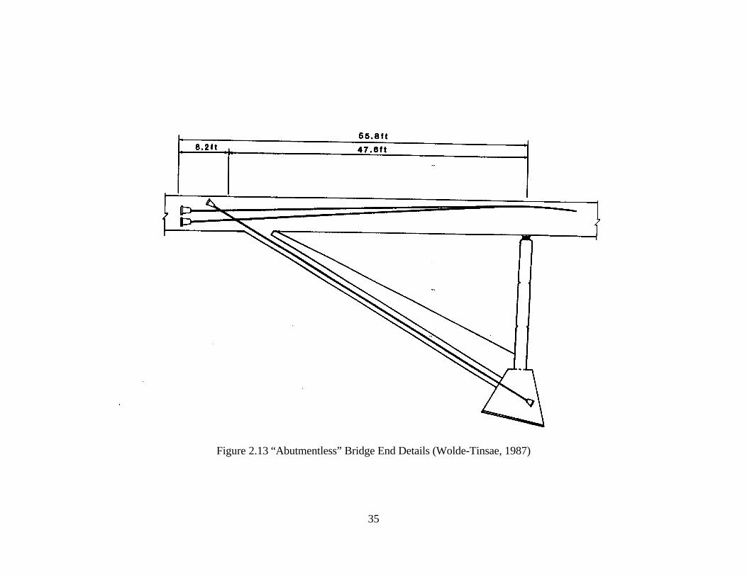
2.9.6 Abutment-less Bridges
Abutment-less bridges are very uncommon in the U.S. However, in Australia eight

30
jointless bridges have been designed without abutments (Wolde-Tinsae, 1987). The elevation and
other details of a typical abutmentless jointless bridge are shown in Figures 2.12 and 2.13. The
bridge end has an unconventional configuration that connects the end of the bridge to the base of
the piers with prestressing strands.
2.9.7 Continuous Jointless decks
The objective of a continuous jointless deck concept is to eliminate as many joints as
possible from the structure. Ideally, all interior expansion joints are eliminated, leaving the only
joints at one or both abutments or approach slabs. Longitudinal movements are accommodated by
a combination of expansion joints and sliding bearings, or by pier flexibility when the
superstructures are rigidly connected to the piers. In addition to the beneficial reduction of
expansion joints associated with this concept, another attribute of superstructure continuity is the
intrinsic reduction of midspan bending moments. This allows the use of more slender sections,
resulting in economical construction, reduced joint maintenance, and a smoother riding surface.
As a result, the continuous jointless deck concept is popular with many highway agencies.
2.10 Retrofit Jointless Bridges
The benefits of continuous construction for jointless bridges lead to a trend of converting
existing multiple span bridges from simple to continuous spans. Freyermuth (1969) gives a rather
complete description of the considerations necessary to achieve continuity in a bridge composed of
a continuously reinforced concrete deck slab on simply supported precast prestressed beams.

31
Figure 2.9 Plan and Elevation Views of 420/QEW Bridge (Wolde-Tinsae, 1987)

32
Figure 2.10 Abutment Sections of 420/QEW Bridge (Wolde-Tinsae, 1987)

33
Figure 2.11 Schematic View of Proposed Jointless Bridge Concept (Zuk, 1981)

34
Figure 2.12 “Abutmentless” Bridge Elevation (Wolde-Tinsae, 1987)
35
Figure 2.13 “Abutmentless” Bridge End Details (Wolde-Tinsae, 1987)

36
Conversion of existing bridges either by a complete deck replacement or by replacing
portions of the deck adjacent to deck joints over piers can be accomplished by following the
procedures developed for new structures. Obviously for existing bridges, creep effects will be
negligible. Shrinkage effects for other than complete deck slab replacements should also be
negligible.
Continuous conversion not only eliminates troublesome deck joints, but also results in a
slightly higher bridge load capacity since positive moments due to live load are reduced by
continuous rather than simple span behavior. The concept of retrofitting jointed bridges to
jointless bridges is gaining impetus in recent years. The effort of converting jointed bridges to
jointless bridges began with Wisconsin and Massachusetts in the 1960's. According to a survey
(Burke, 1990), 11 of 30 transportation departments, have converted one or more bridges from
multiple simple spans to continuous spans.
To give this movement some direction, the Federal Highway Administration has issued a
Technical Advisory on the subject of retrofitting jointed bridges to jointless bridges. The advisory
committee in part recommends that a study of the bridge layout and existing joints be made "...to
determine which joints can be eliminated and what modifications are necessary to revamp those
joints that remain to provide an adequate functional system...". For unrestrained abutments "...a
fixed integral condition can be developed full length of the shorter bridges. An unrestrained
abutment is assumed to be one that is free to rotate, such as a stub abutment on one row of piles or
an abutment hinged at the footing..." where feasible, develop continuity in the deck slab. Remove
concrete as necessary to eliminate existing armoring, and add negative moment steel at the level of
existing top-deck steel sufficient to resist transverse cracking (Figure 2.14a). The detail shown on
Figure 2.14a reflects the procedure adopted by Texas. In this conversion procedure, only the slab

37
portion of the deck is made continuous. The simply supported beams remain simply supported.
For such construction, it is important to ensure that one or both the adjacent bearings supporting
the beams at a joint are capable of allowing horizontal movement. Providing such horizontal
movement will prevent horizontal forces from being imposed on bearings due to rotation of the
beams and slab continuity.
The state of Utah has converted some simple span bridges to continuous ones by using a design
similar to the one shown on Figure 2.14b. For deck slabs with a bituminous overlay, a
waterproofing membrane can be used to waterproof the new slab section over piers. With a design
like this, it is understood that the deck slab would be exposed to longitudinal flexure due to rotation
of the beam ends responding to the movement of vehicular traffic. However, for short and medium
span bridges, the deck cracking associated with such behavior is preferred by some over the long-
term adverse consequences associated with an open joint or a poorly executed sealed joint.
In new construction, conversion of simple spans to continuous spans is rather common.
Figure 2.14c shows the design detail used by the state of Wisconsin for prestressed I-beam bridges.
A concrete diaphragm is placed at piers between the ends of simply supported prestressed beams of
adjacent spans. The diaphragm extends transversely between parallel beam lines. A reinforced
concrete deck slab is placed to integrate the beams and deck slab leading to a fully composite
structure. This type of prestressed I-beam construction appears to be standard for many
transportation departments. Figure 2.14d shows the standard design detail used by the state of
Ohio to achieve continuity for simply supported prestressed box beams. These box beams are
placed side by side and transversely bolted together. Figures 2.15 and 2.16 illustrate design details
used for a number of recent conversions by the ODOT.

38
Figure 2.14 Integral Conversions at Piers (Burke, 1990)

39
Reconstruction of these abutments was necessary because of substantial damage induced
by pavement growth and pressure, deicing chemical deterioration, or both. Instead of replacing
backwalls and joints, and in some cases bearings and bridge seats, it was decided to pattern the
reconstruction after the design details used by the department for its new integral bridges. Thus,
subsequent concern about the effects of pavement pressure and deicing chemical deterioration have
been minimized.
A number of transportation departments have begun to retrofit multiple span steel beam or
girder bridges constructed with intermediate hinges under unsealed deck joints. Figure 2.17 shows
one such example where end span hinges and deck joints (originally intended to accommodate
embankment consolidation and abutment settlement) are replaced with bolted splices and a
continuous concrete deck. Since the structure is more than two decades old and embankments are
essentially fully consolidated, the need for hinges no longer exist.
2.11 Summary
As the trend towards using jointless construction continues, future use of jointless
construction would be standardized. It also appears that the use of integral abutments for single
and multiple span bridges will increase when comprehensive guidelines become readily available,
along with long-term performance data.
Jointless bridges have numerous attributes and few limitations. Since design provisions
can be made to account for some of these limitations (cycle control joints, pressure relief joints,
approach slabs, construction procedures, and structural buoyancy), only application limitations
(structure length, curvature, skew, overburden depth, and unstable subsoils) should negate the use
of integral bridges in favor of the jointed bridges. The high abutment pile stresses and uncertain

40
passive pressure effects are being accepted as the only negative aspects of such designs. However,
these negative aspects are acceptable whenever they are weighed against other attributes that
jointless bridges provide.
The types of jointless bridges are many depending on the superstructure and substructure
configuration, structural requirement, and geographical background. The common purpose of all
types of jointless bridges is to eliminate construction joints. In structural idealization of these
bridges, one should consider all the intrinsic details to correctly assess and appreciate the
performance of jointless bridges. Furthermore, conversion of jointed bridges to jointless bridges is
gaining attention in the process of rehabilitation and strengthening of existing jointed bridges.

41
Figure 2.15 Integral Conversions at Abutments (Burke, 1990)

42
Figure 2.16 Integral Conversions at Abutments (Burke, 1990)

43
Figure 2.17 Integral Conversion at Intermediate Hinge (Burke, 1990)

44
CHAPTER 3
CURRENT DESIGN AND CONSTRUCTION PRACTICES FOR JOINTLESS BRIDGES
3.1 Introduction
As a part of the present research study, a comprehensive review was conducted to
determine the state-of-the-art in jointless bridge design and construction. Several researchers and
research agencies were contacted to obtain a recent knowledge base on jointless bridge design and
construction before conducting this research. A questionnaire (Appendix C) was sent by the CFC
researchers to selected state DOT's (mostly in FHWA Region 3) to understand their perspective on
design and construction of jointless bridges. The information in section 3.5 summarizes the current
design and construction practices for jointless bridges based on the responses by 18 states to a
questionnaire sent by CFC researchers. Section 3.2 summarizes the current AASHTO provisions
for jointless bridges. Sections 3.3 and 3.6 present the state practices as per an earlier survey
(Wolde-Tinsae, 1987) and field performance of a few jointless bridges, respectively.
3.2 Current AASHTO Provisions
The American Association of State Highway and Transportation Officials (AASHTO 1995
and interims) currently provides very few guidelines as to the design of jointless bridges, leaving to
engineer’s judgement details of span length limitations, temperature considerations, foundation
types, backfill material, and approach slabs up to the engineer’s judgement. Section 7.5.3 of
AASHTO Standard Specifications for Highway Bridges states:
Integral abutments shall be designed to resist the forces generated by thermal movements
of the superstructure against the pressure of the fill behind the abutment. Integral abutments
should not be constructed on spread footings founded or keyed into rock. Movement calculations

45
shall consider temperature, creep, and long-term pre-stress shortening in determining potential
movements of abutments.
Maximum span lengths, design considerations, details should comply with
recommendations outlined in FHWA Technical Advisory T5140.13 (1980) except where
substantial local experience indicates otherwise. Maximum span lengths recommended in the
Technical Advisory are 300 feet for steel structures, 500 feet for Cast-In-Place structures, and 600
feet for Pre- or Post-tensioned concrete structures. The Technical Advisory also recommends the
use of approach slabs and minimum approach slab lengths equal to the abutment height plus four
feet. To avoid water intrusion behind the abutment, the approach slab should be connected directly
to the abutment and wing-walls, and appropriate provisions should be made and provide for
drainage of any entrapped water. The Technical Advisory also provides guidelines for abutment,
thermal movement, and approach slab details. However, this Technical Advisory was cancelled in
1989 due to variance in opinion of engineers.
3.3 State Provisions Based on Wolde-Tinsae’s 1987 Survey
3.3.1 Tennessee
Tennessee DOT engineers have had the most extensive experience with jointless bridges in
the United States. Over 1200 integral abutment-type bridges have been built in Tennessee during
the past 25 years, and an estimated 80 percent of all newly constructed bridges in Tennessee were
built without expansion joints. The Tennessee DOT is satisfied with the performance of these
bridges, which in many cases has resulted in immediate cost savings during construction and
reduced maintenance expenditures in the long run.
The efficiency and long-term serviceability of jointless bridges in Tennessee are reflected

46
in their design criteria. For example, the allowable length limits established by the Tennessee
DOT are among the longest currently permitted jointless bridges built by any of the state highway
agencies. The design rationale is based on a maximum expected longitudinal displacement of
about 2 inches at each abutment and expected movements of 0.936 inches per 100 feet of span
(steel bridges) and 0.505 inches per 100 feet of span (concrete bridges). This translates into
allowable lengths of 400 feet for steel bridges and 800 feet for concrete bridges, although these
limits are occasionally exceeded.
The Tennessee DOT has encountered some problems during the development of their
jointless bridges. The typical problems are explained as follows. In one case, an integral abutment
was tied into rock. The resulting lack of flexibility at the abutment caused the bridge to crack at
the end, and part of the necessary repairs included the installation of an expansion joint in the
structure. Bridges currently built on rock or rock fill are founded on piles driven through predrilled
oversize holes or through an earth core in rock embankments to improve the translational
capability of the abutment. Other problems with these bridges were caused by the development of
cracks in the abutments or wingwalls. Although these cracks were considered to be minor and
caused no serviceability problems, careful design of reinforcing steel has effectively eliminated
cracking in these areas.
On-site inspection reports of several jointless bridges in Tennessee indicate no evidence of
abnormal stresses, and these structures appear to be performing as intended. Several instances
have been noted, where settlement and cracking of the approach slabs have been noticed. The
Tennessee DOT expects some eventual localized pavement failure and bumps to develop at the
bridge ends, but considers these problems to be minimal when compared to expenditures and
maintenance efforts necessary to maintain and rehabilitate damaged expansion joints and bridges.
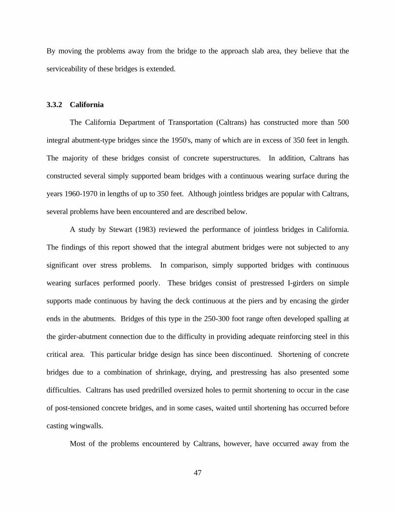
47
By moving the problems away from the bridge to the approach slab area, they believe that the
serviceability of these bridges is extended.
3.3.2 California
The California Department of Transportation (Caltrans) has constructed more than 500
integral abutment-type bridges since the 1950's, many of which are in excess of 350 feet in length.
The majority of these bridges consist of concrete superstructures. In addition, Caltrans has
constructed several simply supported beam bridges with a continuous wearing surface during the
years 1960-1970 in lengths of up to 350 feet. Although jointless bridges are popular with Caltrans,
several problems have been encountered and are described below.
A study by Stewart (1983) reviewed the performance of jointless bridges in California.
The findings of this report showed that the integral abutment bridges were not subjected to any
significant over stress problems. In comparison, simply supported bridges with continuous
wearing surfaces performed poorly. These bridges consist of prestressed I-girders on simple
supports made continuous by having the deck continuous at the piers and by encasing the girder
ends in the abutments. Bridges of this type in the 250-300 foot range often developed spalling at
the girder-abutment connection due to the difficulty in providing adequate reinforcing steel in this
critical area. This particular bridge design has since been discontinued. Shortening of concrete
bridges due to a combination of shrinkage, drying, and prestressing has also presented some
difficulties. Caltrans has used predrilled oversized holes to permit shortening to occur in the case
of post-tensioned concrete bridges, and in some cases, waited until shortening has occurred before
casting wingwalls.
Most of the problems encountered by Caltrans, however, have occurred away from the

48
structure, and involve settlement of the approach slabs and erosion of approach fill, particularly
with longer bridges having integral abutments. A study of the problem by Stewart (1985)
indicated that significant settlement and erosion may occur at the ends of longer bridges after
shortening due to shrinkage of concrete and prestressing has taken place, especially when the
approach slab is constructed with asphaltic concrete. In addition, winter months in California
coinciding with the rainy season led to thermal shortening of the approach pavements and
cracking, thus allowing water to pass freely into the backfill areas.
The settlement and erosion problems, in part initiated by the formation of a gap between
the backwall and fill due to superstructure shortening, may have led to the shear failure of the
abutment paving notch. To counter this problem, a redesign of the paving notch was initiated in
1979 which required additional reinforcement in the shear zones of the notch and areas of the
approach slab adjacent to the notch. The proposed improvement in the notch design did increase
the bearing area of the paving notch from 3 to 6 inches. In addition, a new approach slab policy
was implemented in 1985. This required an addition of a top layer of steel at the approach slab-
bridge deck connection and the extension of the approach slabs over wingwalls to control drainage
and to minimize settlement and erosion.
It is interesting to note that during the 1971 San Fernando Earthquake, bridges with
jointless abutments suffered less overall damage than bridges with conventional seat-type
abutments (Wasserman, 1986).
3.3.3 Iowa
A final report (Greimann, et. al., 1987) on nonlinear pile behavior in bridges with integral
abutments was published by Iowa State University in 1982 under the sponsorship of the Iowa
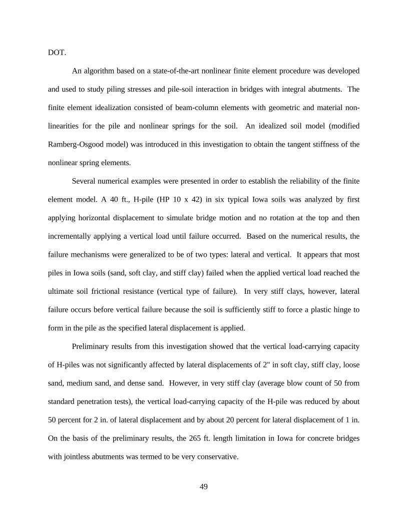
49
DOT.
An algorithm based on a state-of-the-art nonlinear finite element procedure was developed
and used to study piling stresses and pile-soil interaction in bridges with integral abutments. The
finite element idealization consisted of beam-column elements with geometric and material non-
linearities for the pile and nonlinear springs for the soil. An idealized soil model (modified
Ramberg-Osgood model) was introduced in this investigation to obtain the tangent stiffness of the
nonlinear spring elements.
Several numerical examples were presented in order to establish the reliability of the finite
element model. A 40 ft., H-pile (HP 10 x 42) in six typical Iowa soils was analyzed by first
applying horizontal displacement to simulate bridge motion and no rotation at the top and then
incrementally applying a vertical load until failure occurred. Based on the numerical results, the
failure mechanisms were generalized to be of two types: lateral and vertical. It appears that most
piles in Iowa soils (sand, soft clay, and stiff clay) failed when the applied vertical load reached the
ultimate soil frictional resistance (vertical type of failure). In very stiff clays, however, lateral
failure occurs before vertical failure because the soil is sufficiently stiff to force a plastic hinge to
form in the pile as the specified lateral displacement is applied.
Preliminary results from this investigation showed that the vertical load-carrying capacity
of H-piles was not significantly affected by lateral displacements of 2" in soft clay, stiff clay, loose
sand, medium sand, and dense sand. However, in very stiff clay (average blow count of 50 from
standard penetration tests), the vertical load-carrying capacity of the H-pile was reduced by about
50 percent for 2 in. of lateral displacement and by about 20 percent for lateral displacement of 1 in.
On the basis of the preliminary results, the 265 ft. length limitation in Iowa for concrete bridges
with jointless abutments was termed to be very conservative.
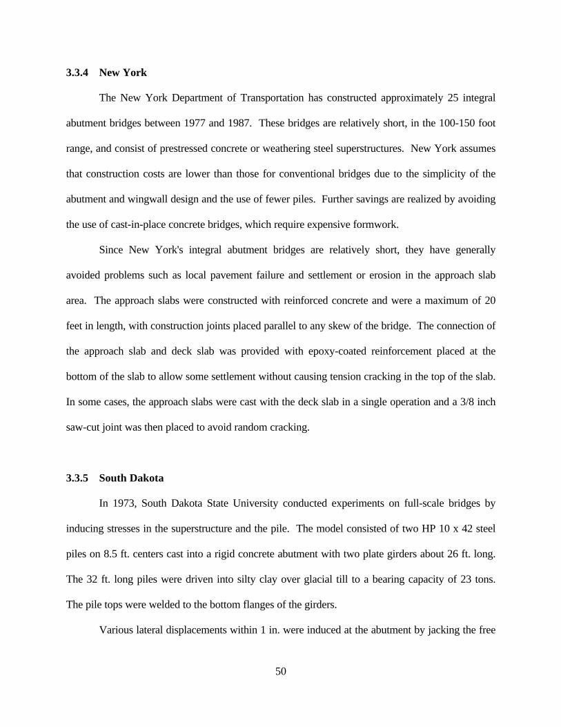
50
3.3.4 New York
The New York Department of Transportation has constructed approximately 25 integral
abutment bridges between 1977 and 1987. These bridges are relatively short, in the 100-150 foot
range, and consist of prestressed concrete or weathering steel superstructures. New York assumes
that construction costs are lower than those for conventional bridges due to the simplicity of the
abutment and wingwall design and the use of fewer piles. Further savings are realized by avoiding
the use of cast-in-place concrete bridges, which require expensive formwork.
Since New York's integral abutment bridges are relatively short, they have generally
avoided problems such as local pavement failure and settlement or erosion in the approach slab
area. The approach slabs were constructed with reinforced concrete and were a maximum of 20
feet in length, with construction joints placed parallel to any skew of the bridge. The connection of
the approach slab and deck slab was provided with epoxy-coated reinforcement placed at the
bottom of the slab to allow some settlement without causing tension cracking in the top of the slab.
In some cases, the approach slabs were cast with the deck slab in a single operation and a 3/8 inch
saw-cut joint was then placed to avoid random cracking.
3.3.5 South Dakota
In 1973, South Dakota State University conducted experiments on full-scale bridges by
inducing stresses in the superstructure and the pile. The model consisted of two HP 10 x 42 steel
piles on 8.5 ft. centers cast into a rigid concrete abutment with two plate girders about 26 ft. long.
The 32 ft. long piles were driven into silty clay over glacial till to a bearing capacity of 23 tons.
The pile tops were welded to the bottom flanges of the girders.
Various lateral displacements within 1 in. were induced at the abutment by jacking the free

51
end during four construction stages. The results of interest concern the stage with the slab and
backfill in place. Strains in the piling corresponding to stresses of up to 42 ksi were measured.
This occurred just below the bottom of the concrete abutment. Several conclusions were drawn by
the investigators, which are presented in the following paragraph:
Stresses induced in the girders due to lateral displacement (in some cases) were additive to
dead and live load stresses. The induced stresses were within 40 percent over stress allowed by the
American Association of State Highway and Transportation Officials (AASHTO).
1) Horizontal movements greater than 0.5 inches cause yielding in the piles.
2) Free-draining backfill was recommended since frozen soil against the abutment can greatly
increase induced girder stresses by limiting free movement.
3) Use of approach slabs was recommended to allow rotation and translation of the abutment and
if possible, avoid continued compaction of the backfill by traffic.
3.3.6 North Dakota
North Dakota was another early user of integral abutments and most of the abutments were
built with concrete superstructures. Current length limits are 300 ft. (steel) and 450 ft. (prestressed
concrete). Jointless bridges in North Dakota have generally performed well, although two
problems were identified with early prototype bridges.
First, the superstructure was originally connected to the backwall with dowel bars that were
placed with insufficient cover. In some places, the concrete over the dowel bars on the inside face
of the backwall cracked due to the thermal forces caused by contraction of the superstructure.
Second, the piles were originally placed with the webs parallel to the longitudinal axis of the
bridge. This orientation caused some distress in the backwall since the piles offered relatively

52
large resistance to lateral bridge movements. The problem was eliminated when the piles were
installed with the webs perpendicular to the longitudinal axis of the bridge.
An interesting design feature was used in the design of one 450-ft. prestressed concrete
bridge with integral abutments built in 1981. A special expansion joint material, which was several
inches thick, was placed behind the abutment backwall. Behind this material was a sheet of
corrugated metal. This detail was designed to reduce passive earth pressures on the abutment and
to help reduce the formation of a void space upon contraction of the superstructure.
3.3.7 Missouri
Missouri was an early user of bridges with integral and semi-integral abutments. Criteria
used in the design of these bridges have been developed primarily from the reported success of
other states, notably Tennessee. The maximum length limits specified in the Missouri Highway
and Transportation Commission bridge design manual were 500 feet (steel, semi-integral
abutment) and 600 feet (prestressed concrete, integral abutment).
In 1972, the University of Missouri conducted a feasibility study of integral and semi-
integral abutments. The following conclusions were drawn from the study:
1) The use of superstructures connected to flexible substructures was becoming generally
acceptable.
2) Design limitations were more restrictive for steel than for concrete bridges.
3) There were no simple design criteria that accounted for shrinkage, creep, temperature, or
substructure flexibility.
4) Induced stresses resulting from thermal effects, creep, shrinkage, backfill movement, and the
like were recognized by bridge engineers as potentially significant, but there is wide variance

53
in methods of considering them.
Bridge design engineers are interested in induced stresses and associated problems.
However, they are generally uncertain as to the significance of and suitable methods for
consideration of these stresses and would welcome a simple, rational design criterion and specific
recommendations as to design details.
3.4 Authors’ Survey of State Practices
As part of the present study, and also to determine the current design practices and trends
followed by different states, a questionnaire (Appendix C) was prepared by the CFC researchers
and mailed to 24 state DOTs in FHWA Region 3. Responses were received from 18 states, a
synthesis of these responses is provided in this section. This survey was conducted with the hope
that bridge designers could use this information to eventually standardize design practices for
integral abutment bridges.
The information furnished by 18 states was synthesized in terms of:
1) Maximum Span Lengths
2) Maximum Skew Angles
3) Presence of Standardized Designs and Design Details
4) Thermal Load Considerations in Design
5) Pile Design
6) Approach Slab Design
An estimate of future integral abutment bridge construction is also included. It should be
noted that if a state is not included in a particular discussion, it means that either the state did not
respond to a question pertaining to the discussion, or the state did not provide enough information

54
in its response to be relevant to the discussion.
3.4.1 Number of Jointless Bridges – Present and Future
Of the 18 responses received, 11 states reported having jointless bridges in service. The
total number of integral bridges in service is over 3200 jointless bridges. Tennessee appears to be
the leader in jointless bridge construction with over 2400 jointless bridges in service. Ohio has
approximately 600 jointless bridges. Of these bridges in Ohio, 580 have steel superstructures,
which are the most number of steel bridges reported. Tennessee reported having approximately
2000 jointless bridges with concrete beams, significantly more than any of the other states
surveyed. The questionnaire responses revealed that 300 to 500 jointless bridges may be built by
13 of these states by the year 2000. Table 3.1 presents the above mentioned data.
3.4.2 Maximum Span Lengths
Most of the states reported having relatively low maximum span lengths for steel beam
bridges of under 200 feet. Three states (Massachusetts, Tennessee and Virginia) reported steel
beam spans over 300 feet. Most of the states surveyed stated that their concrete beam bridges were
limited to less than 150 feet. New York has 128 concrete beam bridges under 116 feet and
Kentucky has 54 concrete bridges under 120 feet. Tennessee has limited the total length of
concrete beam bridges to 140 feet. A few states (Massachusetts, Michigan, Kentucky, Maine and
Virginia) reported concrete jointless bridges with total spans around 300 feet.
3.4.3 Maximum Skew
Many bridges have been skewed due to site constraints and other factors that may not allow

55
a rectangular bridge. Relatively high skews have been reported for concrete beam bridges. Ohio
limits their 580 steel bridges to 30 degrees, as do most of the designers of steel bridges. Skew (in
this study) is measured as the line between the front face of the abutment and a line perpendicular
to the center line of the roadway. Several states seem to be concentrating their efforts on the
designs of either higher spans or higher skews. The states with maximum spans, with some
exceptions, appear to have low maximum skews. For example, Massachusetts and Virginia
reported maximum spans over 300 feet for steel beam jointless bridges, but limited their skews to
less than 30 degrees. Table 3.2 presents the above mentioned data.
New York further sets span and skew parameters based on number of spans for integral
abutment bridges as presented in Table 3.3.
3.4.4 Design and Details
Several states have established their own design criteria. Four of the eighteen respondents
stated that they have used a “standard” design procedure for integral abutment bridge construction.
Pennsylvania, Massachusetts, Tennessee and Michigan reported they have “standard” procedure
for jointless bridge construction. Nine of the eighteen states provided details and guidelines on
integral abutment bridge designs.
For most of the responding states, superstructure design for an integral abutment bridge is
basically the same as the design for a non-integral bridge. West Virginia, Pennsylvania, Maine, and
New York design the superstructure assuming simple supports at abutments and piers. All of these
four states do not consider fixity with the abutment when designing the superstructure. In multi-
span integral abutment bridges, Pennsylvania designs for nearly equal moments in each span, and
Maine designs for nearly equal movement at each abutment.

56
Most states do not have specific design procedures for designing integral abutment bridges,
but accommodate movements at abutments through detailing practices. The design of integral
abutment substructures is governed by dead and live loads, creep, shrinkage and temperature loads
from the superstructure, and earth pressure from the backfill. None of the responding states
consider all of these loads in the design of substructure of integral abutment bridges. Three states
provided some details on the design of the substructure. Pennsylvania, Massachusetts and New
York design abutments for active and passive soil earth pressures using pressure theories (exact
theory not defined by Pennsylvania or New York in their survey responses). Massachusetts
provides an engineering approach to abutment design, which is very extensive and is not offered
by any other state design details provided. Massachusetts has three design considerations in the
design of abutments, which are:
1) When the superstructure longitudinally thrusts one abutment into its backfill the other
abutment must comply by moving away from its backfill.
The abutment backfill, which is resisting longitudinal movement, is capable of mobilizing its
passive resistance. However, at the other abutment only the resistance of the berm can be
mobilized. The resistance of the berm may be neglected due to its limited capacity. The backfill
stiffness should be approximately modeled using one-half of the backfill stiffness at each
abutment. The corresponding backfill forces from the model should be doubled for abutment
design purposes.
2) For the case where the integral abutment geometries and details differ sign-ificantly for a
given bridge, two separate analyses may be required.

57
Approximate number of jointless bridges bysuperstructure typeState Approximate number of
jointless bridges in service Steel beams Concrete beamsNumber of jointless bridges
planned by year 2000Delaware - - - 0
Kentucky 55 1 54 21 to 50
Maine 11 9 2 6 to 20
Maryland - - - -
Massachusetts 15 10 5 21 to 50
Michigan 5 1 4 6 to 20
Minnesota - - - 6 to 20
New Hampshire 2 2 0 6 to 20
New Jersey - - - -
New York 167 39 128 50 or more
North Carolina - - - 6 to 20
Ohio 600 580 20 50 or more
Pennsylvania 5 - 5 50 or more
Rhode Island - - - -
Tennessee 2400 400 2000 50 or more
Virginia 15 14 1 21 to 50
Washington, D.C. - - - -
West Virginia 28 8 20 50 or more
Table 3.1 Summary of Jointless Bridges in Service and Future Trends

58
Steel beam superstructure Concrete beam superstructureState
Max. span Max. skew Max. span Max. skewDelaware - - - -
Kentucky 130' (292'-6" totallength)
0° 120' (402-6" totallength)
30°
Maine 120' (200’ totallength)
15° 80' (330’ totallength)
10°
Maryland - - - -
Massachusetts 350' 30° 278' 30°
Michigan 193' - 310' 39°
Minnesota - - - -
North Carolina - - - -
New Hampshire 153' 20° - -
New Jersey - - - -
New York 163.5' 45° 116' 33°
Ohio - 30° - -
Pennsylvania - - 91' (253' totallength)
15°
Rhode Island - - - -
Tennessee 400' 20° 140' 20°
Virginia 322' 5° 280' 0°
Washington,D.C.
- - - -
West Virginia (320’ total length) 30° (450’ total length) 30°
Table 3.2 Maximum Spans and Skews Reported
Type ofSuperstructure
Maximum Span Maximum Skew
Single Span Two Span Three Span Single Span Multiple Span
Steel 163.5' 132.5' -132.5' 95' - 130' -80'
45° 25°
Concrete 116' 115' - 115' 86' - 86' -52'
57° 4°
Table 3.3 Relation Between Number of Spans and Skews for New York State Integral AbutmentBridges

59
Each separate analysis will assume the full stiffness at the abutment in question and zero
soil stiffness will be assumed at the other abutment.
3) The assumed abutment stiffnesses will require reduction if the resulting forces or
displacements are excessive.
The soil capacity shall be evaluated using accepted modern geotechnical engineering principles.
When the maximum soil capacity is exceeded, the assumed abutment/soil stiffnesses are not
appropriate and shall be adjusted downward, a re-analysis shall be made. This process shall
continue until tolerable soil stresses and displacements are attained.
Further, section 3.4.2.1 of the Massachusetts Highway Bridge Manual describes the
procedure for modeling the abutment as follows: The stiffness of the backfill retained at the
abutments must be estimated to obtain a realistic distribution of forces for integral bridges. The
Design Engineers shall estimate the passive soil stiffness per meter of abutment wall and multiply
this value by the total abutment width to obtain the total passive resistance. The contribution of the
integral abutment pile stiffness shall be added to the abutment soil stiffness to obtain the total
abutment stiffness. Pile stiffnesses may be determined using simplified methods of finding the
equivalent cantilever length. General information, such as the soil classification and relative
density and the pile type, may be used to determine the number of pile diameters to the point of
effective fixity. More rigorous methods shall be used when the soils feature large variations in
stiffness with depth or intermediate layers of soft soils. The stiffness of any piers, which provide
longitudinal restraint, shall be determined so that the total longitudinal stiffness of the structure is
estimated. The following iterative procedure is suggested:
1) Assume unit longitudinal displacement of superstructure;
2) Determine equivalent longitudinal stiffnesses of bridge substructure components which provide

60
longitudinal restraint of substructure for assumed displacement;
3) Determine estimated total longitudinal stiffness of substructures based on assumed
displacement;
4) Determine period of vibration and equivalent inertial force in accordance with AASHTO
criteria;
5) Determine longitudinal displacement from equivalent inertial force and compare with assumed
unit displacement;
6) Repeat steps 2 through 5 until displacement convergence is reached;
7) Determine distribution of equivalent inertial force to component substructures based upon
tributary stiffnesses.
3.4.5 Thermal Load Consideration in Design
Several states agreed that thermal stresses due to expansion and contraction of the
superstructure are very important in the design of an integral abutment bridge. Michigan design
practices accommodate thermal stresses with abutment and abutment backwall movement.
Kentucky designs for thermal bending moments generated at the abutment/ superstructure
connection. New York and New Hampshire state that thermal stresses are accommodated by
flexible piles and sleeper slab movement. Minnesota and West Virginia design the approach slab
joint for thermal movement. West Virginia states that different types of joints accommodate
thermal movement when a flexible pavement is used. Approach slabs are required if thermal
movement is computed to be more than 0.6 inches.
Integral abutments are only used for total thermal movement less than 2 inches. Other
states also limit the use of integral abutments by thermal expansion estimates. Virginia restricts use

61
of integral abutments to thermal movements less than 1½ inches. Maine states that thermal
movement should be less than 1 1/4 inches per 100 feet of deck for steel structures, and less than
3/4 inch per 100 feet for concrete structures. In terms of their maximum spans, this would mean
thermal movement of 2 ½ inches for concrete and steel structures, while Tennessee limits theirs to
only 2 inches. Maine also uses tables to compute the vertical thermal loading on the piles. In the
example design that Maine enclosed with their response, thermal load contributed 23.9% of the
total vertical pile load.
In their designs, Pennsylvania and Tennessee use a temperature change of 120°F for steel
structures to calculate thermal movements. For concrete structures, Pennsylvania uses a 90-degree
change while Tennessee uses a 70-degree change. Tennessee design temperatures are consistent
with AASHTO specifications for all bridges.
Tennessee computes the estimated movement at the abutment/superstructure connection
based on the estimated longitudinal deflection and establish the type of foundation based on this
movement. If necessary, hinged abutments, expansion bearings or different types of foundations
are used. This decision is based on the total anticipated movement of the bridge. Bridge
movements are restricted to 0.505 inches/100 feet for concrete superstructures, and 0.936
inches/100 feet for steel superstructures. This is based on the coefficients of thermal expansion for
these two types of superstructures and is measured from the theoretical center of the bridge. When
the total movement is less than two inches and the abutment is not restrained (free to rotate), no
joint is necessary and the beam is integrated into the abutment, and a construction joint will be
placed between the abutment backwall and the approach slab. Also, expansion joints will be
provided for sidewalks and parapets that pass over the abutment and continue along the approach
slab. When total movement is less than ¼ inch and the abutment is restrained, an integral

62
abutment is used regardless of support type. A strip seal is used for restrained abutment with a
total movement between 1/4 inch and 2 inches, or unrestrained abutment with a total movement
between 2 and 4 inches. A modular expansion joint at the abutment is recommended for a total
movement greater than 4 inches.
3.4.6 Creep Consideration in Design
Creep in a longer span (greater than 100 feet) bridge can add deflection or sag to the
superstructure. Creep stresses are caused by a decrease in the stiffness of the material over time.
For an integral abutment bridge, it means added rotation towards the center of the bridge and
increased moments at the abutment/superstructure interface. However, because of shorter span
lengths of jointless bridges, creep stresses are typically ignored. All of the states responded that
creep stresses are ignored for steel bridges. Only Tennessee stated that creep stresses are
sometimes accounted for in prestressed concrete superstructures.
3.4.7 Substructure Design
Substructures in integral abutment bridges need to be designed to handle vertical loading as
well as moments. The majority of states surveyed stated that bearing piles should be used in
integral abutments. Friction piles and even spread footings were allowed in some special cases.
Some states specify the use of a hinged abutment, where vertical loads are supported by the
substructure, but moments are released at the hinge.

63
3.4.7.1 Pile Design
Piles have been designed to be flexible under forces and moments acting on the abutment.
Three states offer design details on integral abutment piles. New York and Pennsylvania mention
that piles should be designed for vertical and lateral loads and fixity between superstructure and
pile top is ignored. Pennsylvania also states that piles should be analyzed for bending induced by
superstructure movements. Maine provided a step-by-step design procedure for piles.
Typically steel H-piles have been used in the substructure by many states. Concrete and
wooden piles are not used because of flexibility requirements. Some states (Virginia, Pennsylvania
and New York) allow use of concrete encased-steel piles. Pennsylvania and New York specify
that concrete encased piles are not to be used with spans greater that 150 feet. Virginia specifies
only using concrete piles with a shelf abutment, similar to a spread footing on a set of piles.
The majority of the states specified orienting piles on their weak axis, perpendicular to the
direction of movement. Two states specified using strong axis orientation, and other states had
specific criteria for which orientation to use. For instance, New York relates use of axis to length
of span (weak axis for spans less than 90 feet, strong axis for spans greater than 90 feet).
Other details in pile design include embedment depth, overall length of piles, and use of
augured holes. Pennsylvania specifies at least 10 feet of embedment. For Maine, embedment
depth depends on the steel pile used in the design as shown in Table 3.4.
The overall length of piles is relevant to the pile’s flexibility and it’s ability to
accommodate abutment moments. The longer the pile, the more flexible it is. West Virginia
specifies minimum pile lengths of 10 feet, New York specifies 20 feet and Virginia specifies 25
feet. New York specifies 20 feet minimum to “avoid a stilt type effect [piles that do not flex],
provide for scour protection and to provide sufficient lateral support to the pile, particularly since

64
the top 8 feet may be augured and backfilled with sand.”
Augering a pilot hole for some top portion of the pile and then backfilling the hole with
some type of loose backfill material creates a hinge-effect in the substructure. This increases the
flexibility of the piles and the substructure. Massachusetts specifies pre-augering to a depth of 5
feet, New York to 8 feet, Pennsylvania, and Maine to 10 feet. New York backfills this hole with
sand, Massachusetts fills with pea stone gravel, and Maine uses dense gravel. Pennsylvania did not
specify a fill material.
To ensure that the expansion of the deck is compensated for in the abutment, some states
use a pile cap hinge in their design. This hinge allows horizontal movement of the deck, and
rotation of the pile in the direction of movement. Stiffness of the abutment/pile component is
maintained with frictional resistance between abutment and pile cap. Tennessee, Virginia and
Michigan use this in their design details. Designers that do not use this specification usually cause
a hinge below the pile cap by using an augured pile hole.
3.4.7.2 Spread Footings
States were asked to respond to a question on the use of spread footings. Because of
moments and horizontal forces generated in jointless bridges, spread footings are not typically
used. Spread footings do not allow the flexibility that is provided with a pile substructure. States
based their decisions on several different factors such as soil conditions, depth to rock, anticipated
scour and settlement, and thermal movement. Maine offers four parameters for the use of spread
footings. Each of the following parameters must be met in order for a spread footing to be used, as
shown in Table 3.5.

65
Pile Size Minimum Length ofPile into Soil (ft)
HP 10X42 10
HP 12X53 12
HP 14X73 13
HP 14X89 15
Table 3.4 Maine Pile Embedment Length Requirements
Spread Footing is Used if… Is Less Than…
Steel superstructure length 80 feet
Concrete superstructure length 140 feet
Abutment height 8 feet
Skew 25 degrees
Table 3.5 Maine’s Parameters for the Use of Spread Footings

66
3.4.7.3 Wingwall Design
Typically wingwall designs are the same for non-integral bridges as for integral bridges.
All of the states that required wingwalls limited them to 10 feet in length if they are constructed
integral with the abutment. Pennsylvania and New York design wingwalls to be integral with the
main abutment stem as cantilevers over the outer piles or fascia girder. If wingwalls are not
integral with the abutment, they are designed separately to handle lateral loading of the approach
and abutment.
3.4.7.4 Backfill Details
All of the states that responded to this issue agreed that uncompacted backfill should be
used. Some states specified a gradation for their backfill, others specified an optimum moisture
density between 95% and 97% (Pennsylvania specifies both). The weight of this backfill is
calculated and is used in the earth pressure estimate.
3.4.8 Approach Slabs
New York and Pennsylvania require approach slabs in all of their integral abutment
bridges. Pennsylvania specifies 25 feet and New York requires from 10 feet to 20 feet. West
Virginia and Maine provide requirements for the use of approach slabs. West Virginia requires an
approach slab when thermal movement is anticipated to be greater than 0.6 inches. Maine requires
approach slabs for steel integral abutment bridges greater than 80 feet long and greater than 140
feet for concrete structures.
Approach slabs resist movement generated in the abutment. Often a thin plastic layer is
used to permit horizontal movement. Six states specify the use of a filter fabric to allow the

67
approach slab to move freely over the sub base. Massachusetts specifies two layers of 6 mil
polyethylene film, while Virginia specifies 10 mil thick plastic sheet, and Ohio only specifies 2
sheets of film. Pennsylvania requires 2 layers of 4 mil thick polyethylene sheets, and New York
requires 4 mil thick sheets. West Virginia just specifies that some filter fabric be placed prior to
approach slab pouring. In general, these specifications state that when a polyethylene sheet is
used, total thickness should be between 8 and 12 mils.
The approach slab allows longitudinal movement, but only as far as it remains in contact
with the abutment. To keep the approach slab from moving excessively, it is attached to the
abutment and/or rests on a keyed-sleeper slab. It is necessary to have friction between the
approach and the sleeper to restrict rigid body motion of the approach. New York and New
Hampshire specify the use of a sleeper slab in their design details. Tennessee and Virginia use the
sleeper pad in their design details. Sleeper pads are 3 to 5 feet long and run the width of the bridge.
They are similar to a sleeper slab, but have a concrete member protruding up through the deck
(similar to an inverted-T shape). An expansion joint is placed between the concrete of the sleeper
pad and the concrete of the approach slab. Either Styrofoam or neoprene is used to create a small
but effective joint.
Six of the responding states used an expansion joint at the end of the abutment to
accommodate thermal movement. The joints in these bridges are moved out to the end of the
approach slab. Two states (Pennsylvania and Virginia) construct this joint using a neoprene seal,
two states (Tennessee and New York) use a compressible material, one state (New Hampshire)
provides only a gap between the approach slab approach pavement (with a backer rod separating
them), and one state (West Virginia) specified the type of joint to be used.
Kentucky provides a saw cut joint in their design to compensate for transverse expansion in

68
the approach slab. This joint is placed along the centerline of the bridge throughout the length of
the approach slab. In the design details, a 3/8" by 1" construction joint was made and filled with
self-leveling silicone joint sealant. This joint is specified to reduce transverse cracking in the
approach and is only used for cement concrete in the approach slab. New York encountered
problems with this saw cut joint because of approach slab settlement, and therefore does not use it
in its design.
3.4.9 Backwall Design
Virginia states that “backwalls shall be designed to resist passive earth pressure that will
result from thermal movements.” Pennsylvania agrees with this, stating that backwalls and
wingwalls should be designed to resist the “force provided by the movement of assumed wedge of
backfill material in accordance with the passive pressure theory.” To reduce pressures,
Pennsylvania uses a cushion material such as a neoprene sponge or a corrugated metal sheet. The
pressure relieved by this material is not accounted for in the design. Massachusetts and Michigan
use a flexible foam backing material for this same purpose. Three states suggest only the use of a
loose, non-compacted backfill to relieve passive earth pressure. New York suggests designing the
abutment for full passive earth pressure, Tennessee states that the cross-section of the bridge itself
will overcome these pressures, and Minnesota reduces maximum spans and skews to accommodate
earth pressures.
3.4.10 Retrofitting
Six states reported that the problems associated with leaking expansion joints were
eliminated when bridges were retrofitted. The other nine states did not report any previous

69
experience using integral abutment retrofitting. Massachusetts reported modifications to bearings
and seismic retrofitting that was performed at the same time as the joint retrofit. It was estimated
from the responding states that between 95 to 210 retrofits will be performed in these states by the
year 2000.
3.4.11 Cracking
Of the states surveyed, cracking was only reported in three states. Tennessee only reported
cracking in the wingwalls. Because of intense moments and horizontal and vertical loading on the
abutment, cracking could progress faster here (in the wingwall) than in the deck. This would
facilitate costly repairs of the abutment surface and cause alarm as to the feasibility of integral
abutments.
3.4.12 Curved Beams
Another design issue in jointless bridges is the use of curved beams. Some locations
require curved beams to be used because of roadway geometry. Three of the states that responded
specifically stated that only straight beams should be used because of problems of flange buckling.
It should be noted that flange buckling is an issue with jointed bridges as well.
3.5 Performance of Jointless Bridges as Per Wolde-Tinsae, 1987
Although jointless bridges have been built in the United States and other countries since the
1930's, design details and construction procedures have been largely developed on an empirical
basis. In general, modifications of design and construction details have been adopted and
implemented by various state highway departments after a review of the performances of prototype

70
bridges in the field. In the following sections, performance issues of a few jointless bridges found
in the literature (Wolde-Tinsae, 1987) are discussed.
3.5.1 South Fork Putah Creek Bridge
This bridge is located at the Interstate 80/113 interchange about 16 miles west of
Sacramento, California. Built in 1974, this 572 ft. integral abutment bridge consists of continuous
reinforced concrete box girders over six spans. The bridge deck and substructure including piles
were constructed with reinforced concrete, while the approaches were constructed of asphaltic
concrete. The wingwalls were not poured monolithically with the abutments, and the interface
joints were fitted with a neoprene rubber waterstop.
This bridge has been inspected by Caltrans at least once every two years since it has been
in-service. According to the inspection reports provided by Caltrans, some minor pattern of
transverse cracks has been noted in the deck slab in all spans, and one rock pocket at the soffit of a
box girder was patched to protect exposed reinforcing steel. Continued maintenance has been
necessary due to the settlement of the approach slab and erosion in the abutment due to deck
runoff. Several asphaltic concrete leveling courses have been applied to the approaches with
limited success, and the fill erosion has caused the wingwall/abutment joint to separate; thus
tearing the neoprene waterstop.
It was noted in the inspection reports that many of the bridges located near the Interstate
80/113 interchange have been experiencing settlement of the approach fill and erosion of the
abutment fill caused by bridge deck runoff.

71
3.5.2 San Juan Road Overcrossing
This bridge is located on Interstate 80 about 3 miles west of Sacramento, California. Built
in 1970, this 440 ft. integral abutment bridge consists of 4 reinforced concrete box girder spans.
The entire bridge, from deck to piles, was constructed with reinforced concrete. The approach
pavements were constructed with asphaltic concrete.
According to the Caltrans inspection reports for this bridge, deck surface drainage has
entered the approach fill material through sidewalk and gutter joints, causing some erosion and
settlement. Runoff water had also permeated the fill at the approach/deck slab interface, causing
the approach pavement to settle and crack behind the abutment. Routine maintenance of this
bridge includes sealing the joints and cracks with an asphaltic seal.
3.5.3 Holston River Bridge
The Hoslton River Bridge, located near Kingsport, Tennessee, is the longest structure of its
kind to date in the United States. The Holston River bridge has 29 spans, and the jointless deck is
2696 ft. long (southbound lanes) and 2652 ft. long (northbound lanes). The only expansion joints
in the structure are the finger-joints provided at each abutment, where up to 7 inches of movement
is expected to occur.
The superstructure of the Holston River Bridge consists of prestressed concrete box-beam
girders fixed to concrete hammerhead piers, which are expected to accommodate localized
displacements due to thermal loads. Each prestressed concrete girder is 48 inches wide and 54
inches deep, with span lengths up to 105 feet in length.
The prestressed concrete box beams are simple-supported at each pier for dead load and are
made continuous for live load with a diaphragm consisting of precast, prestressed concrete slab

72
panels 3-1/2 inches thick, which are connected to the beams and act as the bottom section of the
deck slab. A cast-in-place concrete deck slab covers the diaphragm to facilitate composite action.
The interior boxes were cast first to reduce creep and shrinkage effects during erection of the
bridge.
An on-site inspection of the Holston River Bridge in 1986, showed that the structure is
performing satisfactorily. Some shrinkage cracks were apparent in the deck slab in the negative
moment regions above many of the piers, and evidence of patching at the girders above the piers
was noted. Preliminary reports show that deck elongation and superstructure stresses have not
reached predicted theoretical levels (Loveall, 1985).
3.5.4 U.S. Route 129 South Interchange
This 400 foot long jointless bridge is located near Knoxville, Tennessee. The bridge
superstructure consists of 2-span continuous steel rolled beams cast into the abutments and the
post-tensioned concrete hammerhead piers. Inspection of this bridge showed that it has performed
well so far. There were no signs of leakage in the abutment and pier areas, and no evidence of
distress at the girder-abutment interface was apparent. Some problems were noted, however, with
the approach slab-deck junction at one end of the bridge, where substantial cracking of the
approach slab had developed.
3.5.5 Route 9 West Over Coeyman's Creek
The Coeyman's Creek bridge, located on the outskirts of Albany, New York, is a single
span, prestressed concrete box girder, integral abutment bridge with an overall length of 107 ft.
The abutments are founded on a single row of piles with rip-rap provided for slope protection. The

73
wingwalls, also founded on piles, are oriented perpendicular to the abutments and are separated by
construction joints.
The deck slab and 15 ft. approach slabs consist of reinforced concrete with a continuous
layer of bottom reinforcing steel. A 4 in. deep saw-cut joint has been provided a few feet behind
each abutment. In addition, the deck slab is crowned to allow runoff water to drain directly into
the creek. Inspection of this bridge showed that it has performed well in-service since 1982. No
evidence of settlement in the approach slab area or erosion of fill was apparent. There were some
minor cracks running parallel to the saw joint.
3.5.6 420/QEW Bridge (Ontario ,Canada)
Concrete bridges with integral abutments, have been built in Ontario since the early 1950's
(Wolde-Tinsae, 1987). Length limits for this type of bridge are 120 feet (precast, prestressed
concrete) and 150 feet (poured-in-place, post-tensioned concrete).
Aside from one notable exception (420/QEW bridge), longer bridges in Ontario are built
with expansion joints, although the number of joints used is kept to a minimum. For recently built
bridges that exceed the length limits given above, a continuous jointless deck is specified in the
design whenever feasible. Almost all the new bridges in Ontario are multispan and are made
continuous for economic reasons and to eliminate deck expansion joints.
3.5.7 Waiwaka Terrace and Kauaeranga Bridges (New Zealand)
New Zealand's experience with jointless bridges began in the 1930's. At first, relatively
short concrete bridges were built with integral-type abutments. By the 1950's, integral abutment
bridges were a commonplace in New Zealand, and standardized design drawings for concrete

74
bridges of this type were developed by the New Zealand Ministry of Works and Development
(NZMWD) for routine use by their bridge engineers.
Although no detailed information concerning the performance of integral abutment
bridges in New Zealand (i.e. bridge inspection reports) was included with the response to the
survey questionnaire (Wolde-Tinsae, 1987), the NZMWD did note that no reports of any problems
with bridges with integral abutments are on file.
The NZMWD found it necessary to strengthen several existing concrete integral abutment
bridges (by prestressing) for exceptionally heavy loads. One of the bridges strengthened in this
manner was the Waiwaka Terrace Bridge, located in New Plymouth. This bridge is a concrete T-
beam integral abutment bridge with an overall length of 152 feet. Although some prestress
shortening was observed during the prestressing procedure, no evidence of cracking or other
distress at the abutments was evident.
A few bridges with semi-integral abutments have been built in New Zealand since the
1960's. A majority of these bridges are built with precast, prestressed 2 cell box concrete units.
The length of this bridge type is usually limited to 230 feet, although the Kauaeranga bridge has an
overall length of 446 feet.
The NZMWD notes that their semi-integral and integral abutments have been very
economical due to the simplicity of abutment design and construction and the elimination of
expansion joints. Although no problems have been reported with the jointless bridges in New
Zealand, the NZMWD has decided to monitor the performance of the Kauaeranga bridge (built in
1986) before increasing length limits of bridges of that type.

75
3.5.8 Jointless Bridges in New South Wales and Queensland (Australia)
The Queensland Main Roads Department (QMRD) has been constructing one type of
precast, prestressed concrete jointless bridge since 1975. With this type of bridge, the precast
simple span slab or box beams are attached to piers and abutments with anchor bolts. Spaces
between beam ends over interior piers are filled with cement mortar, while spaces between beam
ends and subgrade concrete relief slabs at the abutments are filled with compressible material. No
expansion devices are used.
According to the survey response from the QMRD, approximately 200 bridges of this type
have been constructed since 1975. The design of the precast, prestressed girders has become
standardized in Queensland. Typically, the length of these bridges ranges from 130 to 230 ft. The
QMRD is considering increasing the allowable length limit to 328 ft., based on observed behavior
of older bridges and publications that outline experiences with jointless bridges in the United
States.
Since 1963, 49 jointless bridges have been built in New South Wales. Although there are
some exceptions, most of the recently built jointless bridges are widenings or duplications of short
concrete bridges built between 1930 and 1960. Forty one of these bridges have integral abutments
and are built up to the following lengths: 176 ft. (precast, prestressed concrete), 164 ft. (link slab),
89 ft. (poured-in-place concrete), and 63 ft. (steel). The other eight jointless bridges were built
using the so-called "abutmentless" bridge concept in lengths up to 291 ft. Approximately 400
continuous jointless deck bridges have been constructed in New South Wales in lengths up to 2046
ft. (prestressed concrete). Other length limits in this category are 1963 ft. (steel), 1887 ft. (poured-
in-place concrete), and 1116 ft. (steel with continuous concrete slab).

76
CHAPTER 4
FIELD TESTING AND MONITORING OF JOINTLESS BRIDGES
4.1 Introduction
In order to modify existing design procedures and guidelines, three jointless bridges in the
state of West Virginia were field tested and evaluated in the present study. Evaluation of the data
gathered during field monitoring and testing included determination of strength and stiffness
properties, degree of compositeness, degradation rates (if degradation is apparent), load
distribution characteristics. The response of the three bridges to applied loads was compared to the
design-anticipated response to establish the efficacy of the design procedures. In this chapter,
details of loads, bridges and instrumentation used in the present field test are presented.
Load tests were conducted periodically over a two and a half year period to determine
jointless bridge responses. Five load tests were conducted on the McKinleyville bridge, and four
each on Short Creek and Airport Road bridges. Three trucks were used to approximate AASHTO
design loads, and the details of location of the trucks during testing are illustrated in section 4.3.2.
4.2 Schedule of Load Tests and Details of Trucks Used
In all the load tests, three trucks of two different types (tandem and single axle trucks) were
used to approximate AASHTO design loads. Two similar (tandem) trucks were used in all load
cases except the maximum moment case, where three trucks were used (two tandem trucks and one
single axle truck). These (tandem) trucks are designated as 1 and 2, and the dimensions in terms of
tire and axle spacings are as shown in Figure 4.1. Table 4.1 shows details of the load tests, with
truck loadings for each corresponding test.

77
Truck Weight (lbs.)Name ofBridge
Load TestNumber
Numberof loadcases
duringeach test
Date
Truck 1 Truck 2 Truck 3
1 9/12/96 52250 53100 27200
2 7/8/97 56200 52800 34100
3 12/3/97 53700 49400 36200
4 4/14/98 53800 53900 40000
McKinleyville
5
5
10/21/98 53300 52000 35400
1 7/8/97 56200 52800 34100
2 12/3/97 53700 49400 36200
3 4/14/98 53800 53900 40000
Short Creek
4
4
10/21/98 53300 52000 35400
1 7/8/97 56200 52800 34100
2 12/3/97 53700 49400 36200
3 4/14/98 53800 53900 40000
Airport Road
4
4
10/21/98 53300 52000 35400
Table 4.1 Details of Load Tests and Trucks Used

78
Truck Designation (as per section 4.2)
4'-5"
1
1'-10"
7'-6"
13'-1"
Truck Designation (as per section 4.2)
4'-5"
2
1'-10"
7'-6"
13'-1"
Figure 4.1 Tire and Axle Spacings of Tandem Trucks (Truck 1 and 2)
Truck Designation (as per section 4.2)
3
1'-10"
7'-6"
12'-6"
Figure 4.2 Tire and Axle Spacings of Single Axle Truck (Truck 3)

79
The second type of truck, used in conjunction with the maximum positive moment load
case, is typically referred to as a Single Axle truck. The dimensions in terms of tire and axle
spacings for single axle truck are shown in Figure 4.2. These truck diagrams will be used later in
load case diagrams to illustrate their location with respect to stringer location.
4.3 McKinleyville Bridge
The McKinleyville Bridge (WVDOT-DOH Project #S305-27/4-003; Bridge #4076) was
constructed in 1996 over Buffalo Creek near Wheeling, West Virginia. It is a straight, two-lane,
three-span continuous structure with FRP rebar reinforced bridge deck. One half of the bridge
deck is reinforced with sand-coated FRP rebar and the other half of the bridge deck is reinforced
with FRP C-bars. The abutments and parapets are reinforced with typical epoxy coated steel rebar.
The geometric and material properties of McKinleyville bridge are presented in Table 4.2.
These properties are used in the analysis and evaluation of the field data in Chapter 5.
4.3.1 Instrumentation
As stated previously, the McKinleyville bridge was instrumented with over 90 sensors.
These sensors included foil gages on rebar and stringers, embedment gages in the concrete deck,
thermocouple temperature sensors through the depth of the deck and stringers, pressure cells on the
abutment backwall, and vibrating wire gages on the center pile. Figure 4.3 shows locations of foil
and embedment gages in the deck, and the numbering scheme, which will be used later to identify
particular gages and their corresponding strain readings. Figure 4.4 shows the side view of the
gage layout including pressure cells and vibrating wire gages.
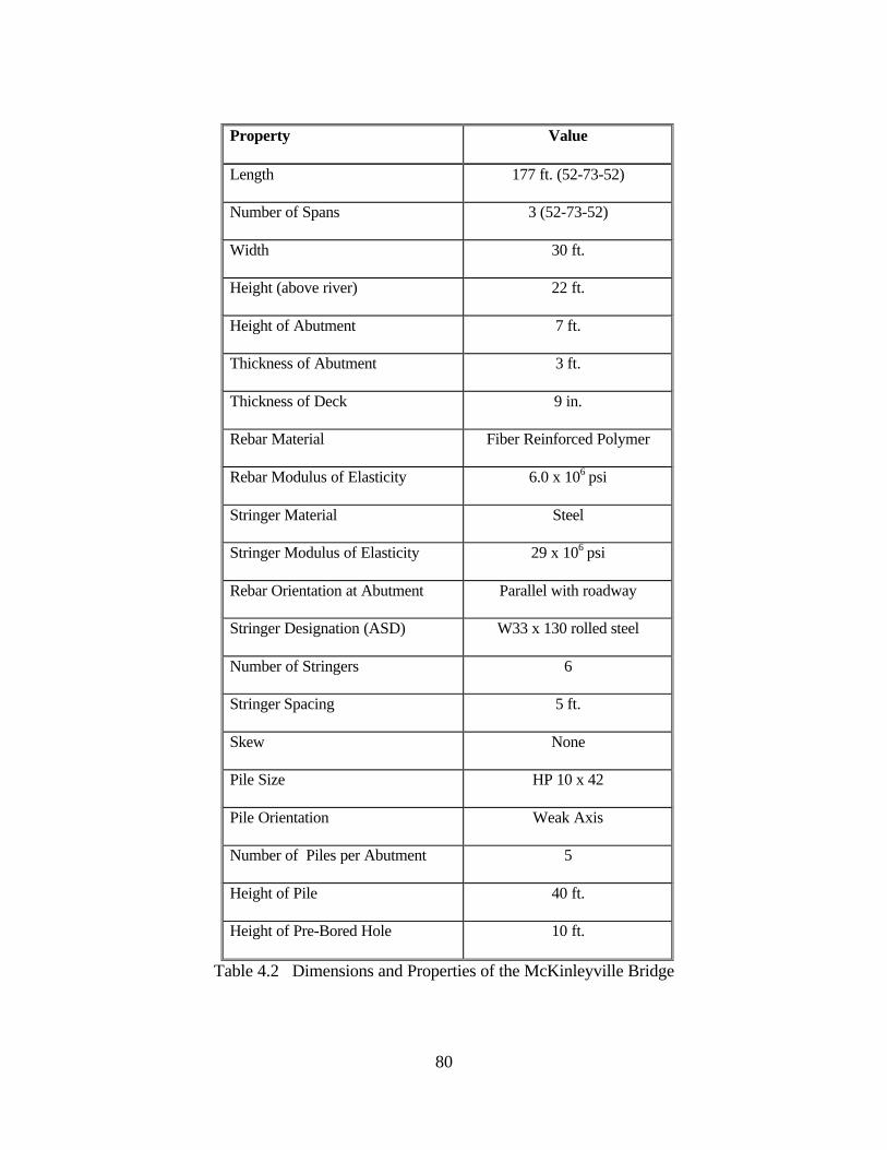
80
Property Value
Length 177 ft. (52-73-52)
Number of Spans 3 (52-73-52)
Width 30 ft.
Height (above river) 22 ft.
Height of Abutment 7 ft.
Thickness of Abutment 3 ft.
Thickness of Deck 9 in.
Rebar Material Fiber Reinforced Polymer
Rebar Modulus of Elasticity 6.0 x 10⁶ psi
Stringer Material Steel
Stringer Modulus of Elasticity 29 x 106 psi
Rebar Orientation at Abutment Parallel with roadway
Stringer Designation (ASD) W33 x 130 rolled steel
Number of Stringers 6
Stringer Spacing 5 ft.
Skew None
Pile Size HP 10 x 42
Pile Orientation Weak Axis
Number of Piles per Abutment 5
Height of Pile 40 ft.
Height of Pre-Bored Hole 10 ft.
Table 4.2 Dimensions and Properties of the McKinleyville Bridge

81
The pressure cells were mounted on the backwall of the abutment at depths of 1 ½ foot, 2
½ feet, 5 feet and 6 feet from the top of the abutment, respectively. The purpose of these cells is to
measure backfill pressure differences as the abutment moves under applied and environmental
loads. The vibrating wire gages were mounted on the web of the pile at depths of 1 foot, 2 feet and
3 feet below the bottom of the abutment. These gages were of the vibrating wire type, where a
metal wire is stretched and plucked and the frequency of the wire is measured. The frequency
determines the strain on the wire. The purpose of these gages is to measure stresses in the pile due
to movement of the bridge superstructure under applied and environmental loads.
To determine the temperature differential, thermocouples or temperature sensors were
placed near both abutments and at midspan, throughout the depth of the deck and stringer.
Deflection measurements were taken to compare with theoretical computations. Global
deflection measurements were taken with the help of a survey crew using a laser level and staff.
Measurements were taken at midspans of Stringer 1, 2 and 3 (see Figure 4.3), at the bottom flange
of the stringer. Only the measurement for Stringer 3 is used for computations (and the only
location displayed in Figure 4.3). Local deflection measurements were taken between Stringers 2
and 3 using a dial gage.
4.3.2 Live Load Cases
Five static live load cases were set up during each load test to determine the effects of
loading at different sections of the bridge. The five load cases are schematically represented in
Figures 4.5 through 4.9. The first load case simulates the maximum possible applied (live load)
moment on the abutment. This load case also induced movement of the abutment and piles, as well
as composite action between the deck and steel stringers at the abutment section. In a jointless or

82
integral abutment bridge the superstructure is “fixed” to the substructure creating an area where
negative moments occur under gravity loads. The magnitude of the moment depends on the
relative stiffness of the substructure in relation to the superstructure. This is not the case in non-
integral and semi-integral bridges where a pseudo-hinge is created.
The second load case (Figure 4.6) causes the maximum negative moment on the
superstructure, i.e. at piers. Because it is a three-span continuous bridge, AASHTO guidelines
suggest loading two of the spans in order to create the maximum negative moment case. The strain
measurements at the cross section (where the maximum negative moment occurs) are extremely
important because concrete is weak in tension, leading to possible deck cracking, spalling or
degradation.
The third and fourth load cases (Figures 4.7 and 4.8) are used to determine transverse load
distribution factors, which are used later to verify the design procedures. Also, load distribution
factors are incorporated in the line girder analysis. The results of line girder analysis are used to
correlate with experimental data.
The fifth load case (Figure 4.9) represents the maximum possible positive moment acting
on the bridge. This load case induces the maximum deflection of the main span, and the maximum
tensile stress on the steel girder as well as the maximum compressive stress acting on the concrete
deck. Results from these load tests are presented in Chapter 6.
4.3.3 Dynamic Load Test
A dynamic load test was also performed on the McKinleyville bridge to determine dynamic
characteristics of the bridge. Details of the dynamic load test are presented in a report available
from the Constructed Facilities Center of West Virginia University (Chen et al. 1997).

83
4.4 Short Creek Bridge
The Short Creek Bridge (WVDOT-DOH Bridge #4050) was constructed in 1993 near
Wheeling, West Virginia. It is a single span, super-elevated bridge, with a 20-degree right-handed
skew. It was chosen for this study because of its close proximity to the McKinleyville bridge.
This bridge receives heavy traffic loading because of a nearby National Guard Base and an airport.
Table 4.3 provides basic dimensions of the Short Creek bridge to compare to the other two bridges
tested and to provide properties used later in this report for analytical calculations.
4.4.1 Instrumentation
Researchers were present at the construction of the McKinleyville bridge, so it was possible
to place sensors inside the deck, behind the abutment and on the piles. Short Creek was already
constructed when this project began so only external measurements were possible.
Foil gages were placed on the steel stringers near the abutment and at midspan. Gages
were placed on the outer three stringers because the bridge is symmetric about the roadway
centerline.
Thermocouples were placed through the deck and along the stringer to measure the
temperature gradient. Holes were drilled in the deck to place thermocouples inside the deck.
For deflection readings, rulers were placed on the midspan stringers and read using a level.
These rulers can be read to 1/64 of an inch, allowing for accurate measurements.
Problems arose that did not allow gages to be placed on the vertical abutment face. For this
reason, a Metzger gage (similar to calipers) was used to measure strains on the abutment face
during loading.

84
Figure 4.3 Gage Layout of McKinleyville Bridge (Plan view)
Figure 4.4 Gage Layout of McKinleyville Bridge (Side View)
13
14
15
4
65
7
9
10
8
1112
3
2
1
23
22
2120
19
V
1817
VI
IV
16
2724
26
25
II
III
I
35
36
34
3233
31
30
29
28
39
38
37
VII
Stringer 3
Pier 2Center of
Location of
Pier 1 Abutment 2
1
Represents gage in top of reinforcement mesh
Represents gage in bottom of reinforcement mesh
Number represent foil gages mounted on sister bars and roman numerals represent concrete embedded gages
Abutment 1
Stringer 1
Stringer 2
Bridge
Global Deflection
Measurement
Location ofLocal Deflection
Measurement
15
56
5350
23
11Abutment 1
Pier 1
4, 7 & 103
6, 9 & 12
15
56
5350
23
11
Pier 1
4, 7 & 103
6, 9 & 12
Pressure
Cells
Vibrating Wire Gages
1.5'
1.0'
1.0'
1.5'
1.0'
1.0'
1.0'

85
Figure 4.5 Maximum Abutment Moment Load Case
1
front faceof abutment
ofpier
Center
ofpier
Center
ofbridge
Center
2
52'
52'
37.5'
37.5'
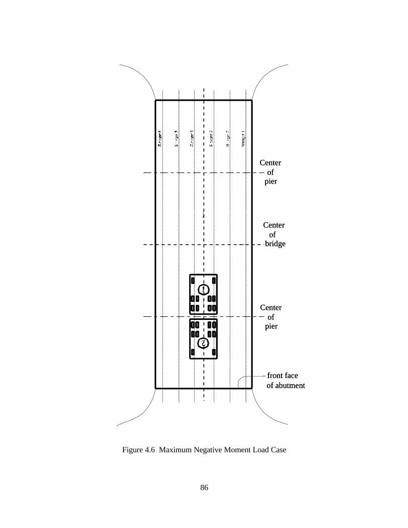
86
Figure 4.6 Maximum Negative Moment Load Case
1
front faceof abutment
ofpier
Center
ofpier
Center
ofbridge
Center
front faceof abutment
ofpier
Center
ofpier
Center
ofbridge
Center

87
Figure 4.7 Transverse Distribution Load Case (right side)
1 2
front faceof abutment
ofpier
Center
ofpier
Center
ofbridge
Center
front faceof abutment
ofpier
Center
ofpier
Center
ofbridge
Center

88
Figure 4.8 Transverse Distribution Load Case (left side)
1 2
front faceof abutment
ofpier
Center
ofpier
Center
ofbridge
Center
front faceof abutment
ofpier
Center
ofpier
Center
ofbridge
Center

89
Figure 4.9 Maximum Positive Moment Load Case
1 2
3
front faceof abutment
ofpier
Center
ofpier
Center
ofbridge
Center
front faceof abutment
ofpier
Center
ofpier
Center
ofbridge
Center

90
The Metzger gage only measures to 12.5 microstrains (10-5), so strain measurements here
were not very accurate.
4.4.2 Load Cases
Four load cases were selected for this bridge, one less than McKinleyville because this
bridge is only single span (the maximum positive and negative moments occur in the maximum
moment load case). The first case (Figure 4.10) induces the maximum moment at the abutment,
which as stated earlier, only occurs in integral abutment bridges. The second (Figure 4.11) and
third (Figure 4.12) load cases are used to determine the transverse distribution factors. The fourth
load case (Figure 4.13) creates the maximum moment on the structure.
4.5 Airport Road Bridge
The Airport Road bridge was constructed in 1994 near Wheeling, West Virginia. It is a
single span, super-elevated bridge, with a 20-degree left-handed skew. This bridge receives heavy
traffic loading because of a nearby National Guard Base and airport.
Table 4.4 provides basic dimensions of the Airport Road bridge to compare to the other
two bridges tested and to provide properties used later in this report for calculations.
4.5.1 Instrumentation
The Airport Road Bridge was instrumented in the same manner as the Short Creek bridge.
There are strain gages on the outer three stringers at the abutment and midspan sections.
Thermocouples were also placed through the deck and along the stringer.

91
Property Value
Length 110 ft.
Number of Spans 1
Width 55 ft.
Height (above river) 32 ft.
Height of Abutment 7 ft.
Thickness of Abutment 3 ft.
Thickness of Deck 8 in.
Rebar Material Steel – Epoxy Coated
Stringer Material Steel
Stringer Modulus of Elasticity 29 x 106 psi
Rebar Orientation at Abutment Perpendicular to roadway
Stringer Designation (ASD) 53 inch plate girder
Number of Stringers 6
Stringer Spacing 8.5 ft.
Parapet Type New Jersey
Skew 20 degrees
Pile Size HP 10 x 42
Pile Orientation Weak Axis
Number of Piles per Abutment 8
Height of Pile 40 ft.
Height of Pre-Bored Hole 10 ft.
Table 4.3 Dimensions and Properties of the Short Creek Bridge

92
1
front faceof abutment
ofbridge
Center
2
Figure 4.10 Maximum Abutment Moment Load Case

93
1 2
front faceof abutment
ofbridge
Center
Figure 4.11 Transverse Load Distribution Case (left side)
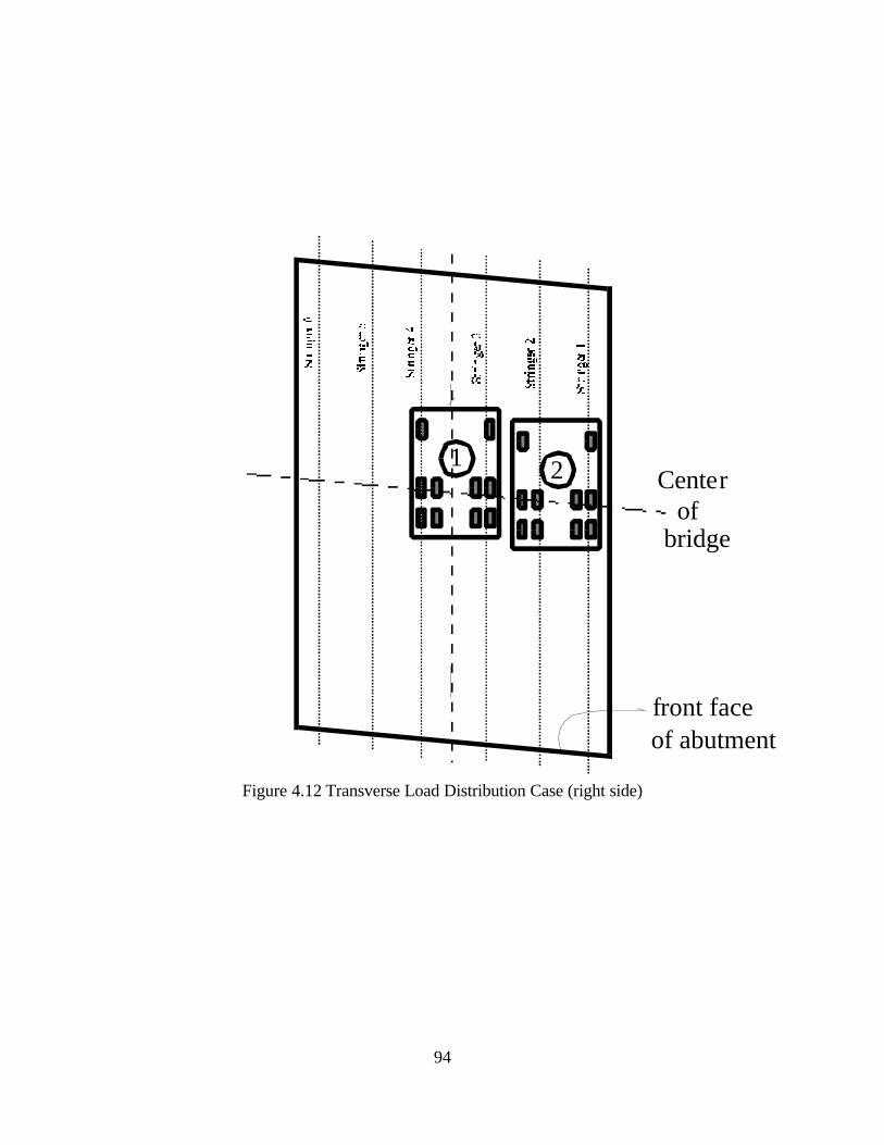
94
1 2
front faceof abutment
ofbridge
Center
Figure 4.12 Transverse Load Distribution Case (right side)

95
1 2
3
front faceof abutment
ofbridge
Center
Figure 4.13 Maximum Moment Case

96
The Metzger gage was also used to measure strains on the abutment for composite action
measurement. Scales and a level were used to measure deflections.
4.6 Load Cases
The load cases for this bridge are the same as for the Short Creek bridge. The first case
causes the maximum moment on the abutment. The second and third cases are used to determine
transverse load distribution factors. The fourth case causes the maximum positive moment in the
bridge.
4.7 Differences Between Short Creek and Airport Road Bridges
The Airport Road bridge is identical to the Short Creek bridge in span length, width and
other component (parapets, piles, abutments, and approach slabs) dimensions and properties. The
major difference between the two bridges is the direction of the angle of skew. Both bridges skew
20 degrees from normal, the Airport Road bridge skew is left-handed (front face of the abutment is
20 degrees counter-clockwise with a line perpendicular to the centerline of the roadway). The
Short Creek bridge skew is right-handed (front face of the abutment is 20 degrees clockwise from a
line perpendicular to the centerline of the roadway).
Another difference between the two bridges is the placement of the transverse rebar at the
abutment, this rebar is perpendicular to the roadway in the Short Creek bridge and parallel to the
abutment face in the Airport Road bridge. The concrete deck near these two abutments will
behave differently with respect to cracking as discussed in section 6.2.
One other difference between these bridges is highway approaches. In the Short Creek
bridge the roadway approach is straight on one end and there is a T-intersection at the other end.

97
In the Airport Road bridge the roadway approaches are both straight. The T-intersection may
affect the continuity behavior of the Short Creek bridge where one end may act as a continuous
beam and the other as a simply support or fixed support in terms of behavior.

98
Property Value
Length 110 ft.
Number of Spans 1
Width 55 ft.
Height (above river) 37 ft.
Height of Abutment 7 ft.
Thickness of Abutment 3 ft.
Thickness of Deck 8 in.
Rebar Material Steel – Epoxy Coated
Stringer Material Steel
Stringer Modulus of Elasticity 29 x 106 psi
Rebar Orientation at Abutment Parallel to Abutment Face
Stringer Designation (ASD) 53 inch plate girder
Number of Stringers 6
Stringer Spacing 8.5 ft.
Parapet Type New Jersey
Skew 20 degrees
Pile Size HP 10 x 42
Pile Orientation Weak Axis
Number of Piles per Abutment 8
Height of Pile 40 ft.
Height of Pre-Bored Hole 10 ft.
Table 4.4 Dimensions and Properties of the Airport Road Bridge

99
1 2
front faceof abutment
ofbridge
Center
Figure 4.14 Load Case 1 Maximum Abutment Moment

100
1 2
front faceof abutment
ofbridge
Center
Figure 4.15 Load Case 2 Transverse Load Distribution (left side)

101
1 2
front faceof abutment
ofbridge
Center
Figure 4.16 Load Case 1 Transverse Load Distribution (right side)

102
1 2
3
front faceof abutment
ofbridge
Center
Figure 4.17 Load Case 2 Maximum Moment

103
CHAPTER 5
RESULTS OF FIELD TESTING AND MONITORING
5.1 Introduction
Three jointless bridges were tested over the period of two and a half years. The field
responses of these bridges were used in developing design procedures and guidelines for integral
(jointless) bridges. Results of load testing along with theoretical calculations for these bridges are
presented in this chapter. Sections are divided to describe response of each bridge, and each bridge
is divided in terms of deflections, strains, temperature gradients and backwall pressures
(McKinleyville bridge only). In addition, transverse load distribution for each bridge was
computed from strain and deflection data. The McKinleyville bridge is discussed first because it
was embedded with many sensors, and had the most field response data. Instrumentation was
completed on the McKinleyville while it was under construction so more measurements (sensors)
and types of measurements were possible from the day of installation. The other two bridges were
already constructed at the start of this project; therefore, only external measurements were possible.
5.2 McKinleyville Bridge Response
5.2.1 Deflections
Deflection measurements were taken during each load test to evaluate the deflection
response of the bridge. These measurements are used to determine design limit states for the
bridge. Limit states are based on responses of the bridge due to predetermined truck loading. Test
vehicles simulated truck load, response was measured.
Global deflection is the vertical deflection of the entire bridge (superstructure) to truck
loading. A level was used to measure global deflections, the smallest measurement possible is 0.01

104
foot or 0.12 inch. This measurement isn’t very precise since global deflection values are of the
order of 0.25 to 0.5 inch for the bridges monitored in this study. Under the field conditions
encountered, levels were the only possible way to get deflection measurements.
Local deflection is the deflection of the deck between stringers due to individual tire loads.
A dial gage was used for local deflection measurement, the smallest measurement possible is about
0.001 inch. This is adequate because estimated local deflection values were of the order of 0.01
inch. These measurements were compared to calculations of deflections using the macro approach
(Chaudhary, 1977), a method used to determine deflections in orthotropic plates. The step-by-step
procedure for finding deflections using macro approach in available in GangaRao, et.al., 1998.
5.2.1.1 Data Reduction
A no load or datum reading was taken prior to loading the bridge with vehicles.
Measurements were taken after subsequent load tests of both dial gage and laser level. These
measurements were compared to the datum reading to find the response in each load case. A no
load reading was also taken after the load tests, which was compared to determine if the deck
bounced back and datum reading was correct.
Locations of wheel loads were marked in relation to stringers and the overall bridge
dimensions. For local deflections, individual wheel loads and their locations between stringers are
important. For global deflections, overall truck placements and their locations on the entire
superstructure are important. These locations are then used to analyze the structure using macro
approach for both local and global deflections. The analytical data are correlated with
experimental data.

105
5.2.1.2 Local (Deck Between Girders) Deflections
Local deflection measurements were taken during five load tests on the McKinleyville
bridge. Each of these load tests included five load cases exhibiting different loadings on the
structure. The maximum positive moment case is used for local deflection evaluation because
loading was in the center of the middle span, away from abutments and piers.
The macro approach was used to obtain theoretical local deflections using tire (patch) load
and locations for the maximum load case. Values obtained are presented in Table 5.1 with
corresponding experimental values.
The local deflection values are normalized for HS-25 loading. The theoretical values
appear differently in each case because truck loading for each case was different. The
experimental trend is showing degradation of the bridge response (80% increase in deflection from
Summer 1997 to Fall 1998) between stringers over time. As explained in later sections, this may
be due to increased transverse cracking of the superstructure. This cracking causes a beam-type
effect on the “local” plate between the stringers, decreasing the effective width of the plate (deck)
so much that it acts like a beam in the transverse direction. A beam deflects more than a
comparable plate because the plate is aided by its transverse directional stiffness. As seen from the
tests following Summer 1997, the local deflection is increased approximately two-fold. Other
effects of increased cracking are discussed in Section 6.2.
Comparison of the theoretical local deflection calculation to experimental values taken in
Summer 1997 reveals a six percent difference. The deck degradation was minimal up to the first
load test. The comparison between the experimental and theoretical values are larger for the other
load tests because the deck cracking effects (after two years in service) are not incorporated.

106
Local Deflection (inch) % Differencebetween Theory and
Experiment
Theoretical
Source
FullEffective
DeckWidth
50% ofEffective
DeckWidth
Experimental FullEffective
DeckWidth
50% ofEffective
DeckWidth
% DeckDegradation
AASHTO L/500 ininches (prorated)
Fall 1996 load test -- -- N/A -- -- -- 0.0768Summer 1997 load test 0.0067 0.0134 0.0071 6.0 88.7 -- 0.0768Winter 1997 load test 0.0055 0.0110 0.0098 78.2 12.2 38.0 0.0768Spring 1998 load test 0.0075 0.0150 0.0118 51.3 27.11 74.6 0.0768
Fall 1998 load test 0.0063 0.0126 0.0114 80.9 10.5 80.3 0.0768Table 5.1 Local Deflection of McKinleyville Bridge for Maximum Positive Moment Case
Global Deflection (inch)SourceTheoretical Experimental
% Difference betweenTheory and Experiment
AASHTO L/1000 ininches (prorated)
Fall 1996 load test -- N/A -- 0.56Summer 1997 load test 0.35 0.36 2.9 0.56Winter 1997 load test 0.34 0.36 5.9 0.56Spring 1998 load test 0.36 0.36 0.0 0.56
Fall 1998 load test 0.35 0.36 2.9 0.56Table 5.2 Global Deflection of McKinleyville Bridge for Maximum Positive Moment Case

107
However, cracked moment of inertia analysis can yield more accurate theoretical
comparisons with field data, by considering only half of the effective deck width, used in earlier
calculations, as the effective deck width for local deflection computations. The full effective width
is 2/3 of the spacing between stringers. The half effective deck width comparison for the other
three load tests shows a good comparison with experimental values as shown in Table 5.1.
Experimental values are well within AASHTO L/500 (where L is spacing between
stringers) limits for local deflections of urban bridges.
5.2.1.3 Global (Stringer) Deflections
Global deflection measurements were taken during five load cases of five load tests on the
McKinleyville bridge. Again, the maximum positive moment case is used for comparison
purposes. However, it is used because this bridge is treated as a single-span simply-supported
bridge for design simplicity with effective lengths for center and exterior spans. The maximum
global deflection occurs at the middle of the center span of the bridge.
The macro approach was used to obtain theoretical values for global deflections for the
maximum positive moment load case (Figure 4.9). Values obtained for deflections are presented
in Table 5.2 with corresponding experimental values. Theoretical calculations compare very well
with these experimental results. It should be noted that only measurements in 0.12-inch
increments, i.e. 0.24, 0.36 and 0.48 inch, are possible because of instrumentation.
Local deflections in section 5.2.1.2 showed an increase in local deflection due to
progressive deck microcracking, while global deflections (Table 5.2) show very little increase. As
stated in section 5.2.1.2, increased local deflection may be due to transverse cracking of concrete.

108
Since steel stringers take most of the loading of the overall structure, the global deflection may not
change much due to local cracking of the concrete deck.
Experimental values are within AASHTO L/1000 (where L is the span length of the bridge)
deflection limits for urban bridges.
5.2.2 Strain
Strain measurements are useful in determining stresses in members and verify design
procedures. Strains are directly related to stresses through Young’s Modulus. Strain gages were
placed at critical points in the superstructure and on the piles. In the superstructure, gages were
placed on top and bottom levels of the reinforcement mesh in both transverse and longitudinal
directions (Figure 4.3). A data acquisition system was used to acquire data from 60 strain gages
(39 rebar gages, 7 concrete embedment gages, and 12 stringer gages) in the deck. This allowed
eight readings to be taken at one time and increased the number of load cases possible (decreased
the amount of time needed for each load case).
Gages were also placed on the bottom flange of steel stringers at the center of the first two
midspans and near (one foot from) the first abutment and first pier. Gages were placed on the
outer three stringers because the bridge is symmetric about the centerline of the roadway. The
strain data are useful to verify deflection measurements and validate design procedures. Moments
can be determined from a line girder analysis (Appendix B), which can be used to determine
stresses on the structure. These theoretical stresses are compared to stresses determined from
experimental/field strain data.
Gages were placed on the piles to determine the bending stresses in piles due to
superstructure movement under applied and environmental (thermal, pile movement, and

109
passive/active backfill pressure) loading. In an integral (jointless) bridge, the superstructure is cast
directly into the abutment, which rests on piles. The bridge now acts like a frame rather than a
beam as in simply-supported structures. The piles are now the “wobbly” legs of the frame, being
cast into the abutment (or pile cap) and driven deep into the soil. Researchers are unsure of pile
movement and effects on these bridges. Typically, piles are surrounded by soil on all sides and
typically have nothing supporting them. Therefore, field strain data help determine the behavior of
the pile under applied and environmental loading on the superstructure.
5.2.2.1 Data Reduction
Strain gage readings were taken during all five load tests and all five load cases of each
load test. Strain values for the stringer and deck gages were extracted from the data acquisition
system when the testing took place. Pile gages were read with a vibrating wire readout box, which
also read the temperature of the gage. The strain is then calculated using the value from the
readout box and is calibrated for appropriate temperature.
5.2.2.2 Deck strains
Concrete environment can be very harmful to electrical equipment, especially when the
concrete is hardening. Concrete and water can invade any opening and wreak havoc on strain
gages and wiring. Precautions were taken to ensure that gages would survive the curing process,
but several gages did not survive the harsh concrete environment. Other gages were stepped on or
ruined during construction and pouring of the concrete deck. For these reasons, a specific set of
gages (ones that were working) is used in discussing deck strains from the field data. All of the
gages over the third girder survived, so they will be used in this discussion.

110
Analytical calculations were made based on truck loads, distribution factors and bridge
dimensions using a line girder analysis to determine theoretical strains for each load case. The
third girder is the “line girder” used in this approach because all of the gages over the third girder
survived. Strains in the deck for the maximum positive, negative and abutment moments are
shown in Tables 5.3, 5.4 and 5.5 respectively (note: only 4 load tests are shown because values
were not available for the first load test due to malfunctioning of instruments). Theoretical values
are based on a moment of inertia of 13197 in4 (for 50% compositeness) and an effective span
length of 65.7 feet (0.9 time the span length of 73 feet). Refer to Chapter 4 for gage numbering.
Comparing experimental values between load tests for each gage, Gage 3 does not appear
to be affected by temperature changes. The four load tests listed in Tables 5.3 through 5.5 are
during summer, winter, spring and fall, so a definite temperature difference would exist between
load tests. In fact, most of the gages, except Gage 15 appear to be relatively unaffected by
temperature changes. There is a trend showing up in some gages, that higher strains occur in
warmer temperatures than in colder temperatures. Overall, strains do appear to be decreasing
slightly over the course of time.
Only general conclusions can be drawn from these results, i.e., strain values do not match
well with theory, but a trend definitely exists. For Gage 3 at the abutment, it is showing that
theoretical values are high (2 to 3 times) for maximum positive and abutment moment cases.
Theoretical values are low for maximum negative moment case, even to make any
intelligent/accurate comparison with experimental data.
Comparing theoretical to experimental values for Gage 11 at the first midspan, the trend for
maximum positive moment case is showing 50% lower value than in summer and winter and 50%
higher in spring and fall. This suggests that temperature effects have some bearing here. For the

111
maximum negative case, theoretical values are near zero, while experimental values vary greatly,
therefore no trend exists here. For the maximum abutment moment case, theoretical values appear
to be 4 times lower than experimental values. Constant values here suggest that temperature has
no effect on load response at the abutment, where a vehicle first enters the bridge.
Comparing theoretical to experimental maximum positive moment strains for Gage 15,
over the first pier, theoretical values are about 50% low for all seasons. Maximum negative and
abutment strains are showing that summer and winter values are approximately 1.5 to 2 times
lower than experimental values, while spring and fall values are 5.5 to 6 times lower than
experimental values.
No trend exists for Gage 23, at midspan, for the maximum positive moment case.
Maximum negative and abutment moment cases, however, are showing a decent comparison.
Overall comparison between theoretical and experimental deck strain values are not very
good. Two main reasons for this are (1) all computations are for 50% compositeness, but the deck
seems to be degrading over time, and (2) transverse and longitudinal cracks (the source of the
degradation) are increasing in number and appearing randomly (a crack may appear in one location
and not another, i.e., the section properties of the deck cannot be “smeared” over the entire bridge
under analysis) over time. Also, it should be noted that it is not proper to compare low range
"absolute" experimental values because of instrumentation inaccuracies at low ranges.
5.2.2.3 Stringer Strains
Strain values from stringer gages were also acquired using the data acquisition system.
These strain data were processed by the system and shown in Tables 5.6, 5.7 and 5.8.

112
Test Date Summer 1997 Winter 1997 Spring 1998 Fall 1998Gage Theory Experiment Theory Experiment Theory Experiment Theory Experiment
3 9 15 10 8 11 0 10 011 -19 -44 -20 -12 -23 -39 -21 -1115 -86 -142 -92 -156 -103 -147 -96 -11923 81 25 86 6 97 275 90 25Table 5.3 Deck Microstrains for Maximum Positive Moment Case (Figure 4.9)
Test Date Summer 1997 Winter 1997 Spring 1998 Fall 1998Gage Theory Experiment Theory Experiment Theory Experiment Theory Experiment
3 0 3 0 2 -1 2 -1 -411 1 41 1 17 2 0 1 615 -28 -34 -28 -116 -31 -73 -28 -3323 1 1 1 -2 1 74 1 1
Table 5.4 Deck Microstrains for Maximum Negative Moment Case (Figure 4.6)
Test Date Summer 1997 Winter 1997 Spring 1998 Fall 1998Gage Theory Experiment Theory Experiment Theory Experiment Theory Experiment
3 -9 3 -9 -4 -11 0 -10 311 10 41 10 34 11 39 10 4115 -12 -34 -12 -71 -13 0 -12 -3423 -2 1 -2 0 -2 0 -2 1
Table 5.5 Deck Microstrains for Maximum Abutment Moment Case (Figure 4.5)

113
Comparing experimental values between each load test, values appear to be peaking in the
Spring 1998 load test. Values start out lower in Summer 1997 when compared to the peak value,
Spring 1998, and then decrease to values of Summer 1997.
Overall the experimental values appear to be reaching the theoretical values over time. The
theoretical values are based on 50% compositeness, and the deck, because of cracking, appears to
be degrading to this value (50% contribution of concrete deck).
Comparing experimental to theoretical values from line girder analysis for Gage 50, at the
abutment, theoretical values are showing that the strain should remain constant, but experimental
values are showing a significant increase in fall and spring for maximum positive moment case.
Maximum negative strains show no trend, while maximum abutment strains show slightly higher
values for theory than experiment, except for the erratic value for spring.
For Gage 53, at first midspan, the maximum positive experimental strains seem to be
building up to match theoretical values. For maximum negative theoretical strains, values appear
to be 10 times lower in spring and fall, and 6 times lower in summer and winter compared to
experimental values. Values are relatively close for maximum abutment, but no trend exists.
Gage 56 seems to validate Gage 53, wherein experimental values are building up to match
theoretical values. For maximum negative moment, theoretical values are 7 times higher in
summer and winter and 2 times higher in spring and fall. A slight trend exists for maximum
abutment moment where summer and winter values are 3 times higher, but spring and fall values
are unrelated.
Maximum positive strains for gage 59 are approximately 50% lower, while negative
moment values are close to theoretical. However, abutment moment values are 4 times lower than
theory.

114
Test Date Summer 1997 Winter 1997 Spring 1998 Fall 1998Gage Theory Experiment Theory Experiment Theory Experiment Theory Experiment
50 23 18 24 45 27 40 25 1953 -95 -25 -101 -59 -114 -119 -105 -10856 -212 11 -227 -120 -255 -196 -236 -19759 399 -- 427 262 480 317 444 346
Table 5.6 Stringer Microstrains for Maximum Positive Moment Case
Test Date Summer 1997 Winter 1997 Spring 1998 Fall 1998Gage Theory Experiment Theory Experiment Theory Experiment Theory Experiment
50 -1 -18 -1 -11 -2 0 -1 -353 5 29 4 40 8 80 7 3856 -68 -11 -68 28 -77 -40 -69 -1259 6 -- 6 8 5 0 5 16
Table 5.7 Stringer microstrains for Maximum Negative Moment Case
Test Date Summer 1997 Winter 1997 Spring 1998 Fall 1998Gage Theory Experiment Theory Experiment Theory Experiment Theory Experiment
50 -23 -18 -23 -18 -26 -39 -24 -1853 49 29 49 38 56 73 50 2956 -29 -11 -29 -26 -33 -79 -29 -1159 -10 -- -10 -38 -11 -39 -10 --
Table 5.8 Stringer Microstrains for Maximum Abutment Moment Case

115
The maximum observed experimental strain value was 346 microstrains at the bottom of
Stringer 3. The effective load coming from the three trucks (around 50 kips) on Stringer 3 is more
than AASHTO HS-25 design truck loading (90 kips/2). The stress, including impact,
corresponding to 346 microstrains is around 13 ksi, which is well within the allowable stress for
steel.
5.2.2.4 Pile Strains
Readings on piles were taken periodically, as well as during load tests. Values for the load
tests are presented in Tables 5.9, 5.10 and 5.11. Theoretical values are determined by treating the
bridge as a 2-dimensional frame (line girder), the same analysis used for superstructure strains
except the abutment and piles are added to the structure being analyzed. The span length and
moment of inertia used are the same as stated in Section 5.3.1.2.
Comparing experimental values between load tests, all three gages appear to behave
differently under temperature changes. Gage P1, the topmost pile gage, would have maximum
strains in summer, decrease in fall, decrease more in winter, increase slightly in spring and return
to maximum in summer. Gage P2, the middle pile gage, would remain relatively unchanged
during the year. Gage P3, would have maximum strains in spring, slightly decrease in fall, reach
minimum in winter, increase in summer and return to maximum in spring.
Similar trends exist for all three pile gages when comparing theory to experiment. For the
maximum abutment moment case, theory suggests the strains should be increasing more rapidly
than the actual occurrence. The lowest (with respect to depth) gage (P3) showing differences in
values around 4 times too high. For maximum negative case, strain values are reasonable and very
close to experimental values and a definite trend exist.

116
Additional measurements were also taken periodically with no live load on the structure,
these results are shown in Table 5.12.
The initial reading taken before the deck was poured shows that there was an increase of
roughly 130 microstrains (3.77 ksi in terms of stress) due to increased dead load on the structure
(from the deck that was poured). This strain is now locked-in the pile and will always be present,
as evident from Table 5.12.
5.2.3 Temperature Gradients
All materials have thermal coefficients that determine how much that material
expands/contracts for different temperature fluctuations. An integral (jointless) bridge acts like a
frame and the superstructure is restricted from free horizontal movement because it is tied directly
to the abutment and substructure. Thermal expansion of the restricted superstructure can cause
stress build-up at the abutments and in the superstructure. Therefore, to determine stresses caused
by thermal expansion the temperature gradient was measured. This shows the differences in
temperature in the superstructure along its depth. Different expansion rates of concrete and steel
cause moments that are made equivalent to actual loads (equivalent to prestress) on the structure in
the design.
The temperature gradient of the McKinleyville was measured for summer and winter to
establish gradients along the stringer-deck depth which is used in the temperature induced stress
analysis of design. This gradient is representative of this area and is only displayed here to show
the gradient that can occur in the field. Temperature gradients for summer are given in Table 5.13
and for winter in Table 5.14. We see from the tables that the winter temperature gradient is lower
than the summer, this may be due to solar radiation or other factors.

117
Test Date Summer 1997 Winter 1997 Spring 1998 Fall 1998Gage Theory Experiment Theory Experiment Theory Experiment Theory ExperimentP1 48 39 51 32 58 35 53 31P2 80 34 86 37 96 37 89 35P3 112 40 120 40 135 43 125 39
Table 5.9 Pile Microstrains for Maximum Positive Moment Case
Test Date Summer 1997 Winter 1997 Spring 1998 Fall 1998Gage Theory Experiment Theory Experiment Theory Experiment Theory ExperimentP1 -2 -5 -2 -7 -4 -4 -3 -3P2 -4 -2 -3 -1 -6 -3 -5 -2P3 -5 -10 -4 -2 -9 -11 -7 -10
Table 5.10 Pile Microstrains for Maximum Negative Moment Case
Test Date Summer 1997 Winter 1997 Spring 1998 Fall 1998Gage Theory Experiment Theory Experiment Theory Experiment Theory ExperimentP1 -49 -39 -49 -17 -56 -33 -50 -27P2 -82 -35 -82 -19 -94 -28 -84 -31P3 -115 -31 -116 -24 -131 -35 -117 -36
Table 5.11 Pile Microstrains for Maximum Abutment Moment Case
Reading DateGage 7/1/96 9/12/96 4/23/97 7/8/97 4/14/98 10/22/98
P1 0 -136 -162 -182 -151 -131P2 0 -138 -165 -178 -156 -134P3 0 -159 -186 -204 -157 -137
Table 5.12 Pile Microstrain Readings Over Time

118
Depth (inch) Location Temperature (°F)
42.49 Bottom of Steel Stringer 0 (datum)
39.49 Web of Steel Stringer 1
33.49 Web of Steel Stringer 1
27.49 Web of Steel Stringer 2
21.49 Web of Steel Stringer 3
18.49 Web of Steel Stringer 4
12.49 Web of Steel Stringer 5
8 Bottom Mesh of Reinforcement 8
1.5 Top Mesh of Reinforcement 12
Table 5.13 Summer Temperature Gradient for McKinleyville Bridge
Depth (inch) Location Temperature (°F)
42.49 Bottom of Steel Stringer 0 (datum)
39.49 Web of Steel Stringer 1
33.49 Web of Steel Stringer 1
27.49 Web of Steel Stringer 2
21.49 Web of Steel Stringer 2
18.49 Web of Steel Stringer 3
12.49 Web of Steel Stringer 4
8 Bottom Mesh of Reinforcement 7
1.5 Top Mesh of Reinforcement 10
Table 5.14 Winter Temperature Gradient for McKinleyville Bridge
Depth TheoreticalPressure withSurchage (psi)
TheoreticalPressure WithoutSurcharge (psi)
Summer1996
Fall1996
Winter1996
Spring1997
Summer1997
Spring1998
Fall1998
0 0 0 0 0 0 0 0 0 01.5 19.99 12.19 11.98 3.84 5.76 8.67 11.24 7.88 3.993.5 39.96 28.44 12.99 7.89 8.97 10.36 13.65 9.56 7.574.5 47.36 36.56 11.68 9.57 8.79 11.42 12.63 11.35 8.79
6 57.53 48.75 16.42 14.33 14.99 14.39 15.12 13.99 13.30Table 5.15 Backfill Pressures in psi for McKinleyville Bridge

119
5.2.4 Backwall Pressures
Pressure on the back wall of the abutment was measured periodically as well as during load
testing. Pressure cells were installed on the abutment before backfill was placed so readings and
pressure values are with respect to a zero pressure datum. Readings did not change during load
testing, primarily because the abutment backfill is loose. Pressure on the backwall changed over
time and an initial increase occurred due to the fill placement.
Figure 5.1 better illustrates the trend here; summer values are highest and winter values
lowest. In summer the deck expands (due to thermal expansion) and forces the abutment against
the backfill, thus increasing the pressure behind the abutment (where the pressure cells are
located). Pressure near the bottom of the abutment remained relatively constant over time, being
slightly higher in summer. Pressure toward the top of the abutment (at 1.5 foot depth) was
maximum in the summer and minimum in the fall, spring was slightly higher than winter. This
also shows that the movement is in the deck (superstructure), and is due to thermal expansion.
Summer values are 3 times higher than fall values. Overall, pressure on the abutment appears to
stay within the limits of summer and fall and does not appear to be going beyond these values.
Theoretical calculations were made based on Rankine Earth Pressure theory (Das, 1990). A
surcharge was also calculated to compensate for the approach slab that is tied directly to the
abutment. These values are presented in Table 5.15 and Figure 5.2. Calculated values are much
higher than measured, this may be because the backfill is looser than anticipated.
The backwall pressures illustrated in Figure 5.1 can offer insight as to the behavior of the
abutment and piles during a yearly temperature cycle. Keep in mind that throughout the cycle
shown, that the deck is cracking and degrading over time.

120
Pressure vs. Depth Over Time
0
2
4
6
8
10
12
14
16
18
0 2 4 6 8
Depth (feet)
Pre
ssu
re (
psi
)
Summer 1996
Fall 1996
Winter 1996
Spring 1997
Summer 1997
Spring 1998
Fall 1998
Figure 5.1 Backwall Pressure of McKinleyville Bridge Over Time

121
Pressure vs. Depth Over Time
0
10
20
30
40
50
60
70
0 2 4 6 8
Depth (feet)
Pre
ssu
re (
psi
)
Pressure WithSurchagePressure WithoutSurchargeSummer 1996
Fall 1996
Winter 1996
Spring 1997
Summer 1997
Spring 1998
Fall 1998
Figure 5.2 Backwall Pressure of McKinleyville Bridge with Theoretical Pressure Comparison
THEORY
EXPERIMENT

122
The values, based on season (summer, winter, etc.) are very close in magnitude, and do not
appear to be affected by deck degradation. The uneven pressure diagram in summer (dip at 4.5
feet and rise at 6 feet) seem to relate that the abutment is flexing and experiencing different
pressures at different depths. This is due to thermal expansion of the deck, which acts on the top of
the abutment. In fall 1998 there appears to be insignificant passive pressure effects (straight line
diagram), further supporting that temperature expansion is the reason for the increase in pressure at
the top of the abutment in summer.
5.2.5 Transverse Load Distribution Factor
When a vehicle crosses a bridge, its load is transferred through the deck and is distributed
to individual stringers in the transverse direction. Load distribution factors are determined for
bridges, then used in the design to determine individual moments on stringers due to design truck
loads. Transverse load distribution is better for jointless bridges because the effective span of the
bridge is lowered due to partial fixity at the abutments.
Vehicles were placed on the bridge at the midspan to cause an eccentric load condition.
Strains and deflections were measured and used to calculate transverse load distribution factors.
The percentage of strain on the individual stringer in relation to the total strain (sum) on all
stringers determines the distribution factor. In design, distribution of design loads on both interior
and exterior girder are needed for their design. Analysis of the interior girder distribution factor is
accomplished using the maximum positive moment load case (Figure 4.9 for McKinleyville
bridge). Reciprocal theory is used to simulated symmetric conditions, since individual tire loading
may vary.

123
Load Distribution FactorSource Interior Girder Exterior Girder
AASHTO 0.455 (S/5.5) 0.455AASHTO-LRFD 0.445 (S/5.62) 0.367Fall 1996 load test N/A N/A
Summer 1997 load test 0.37 (S/6.76) 0.295Winter 1997 load test 0.392 (S/6.38) 0.307Spring 1998 load test 0.436 (S/5.73) 0.264
Fall 1998 load test 0.387 (S/6.46) 0.314Table 5.16 Load Distribution Factors for McKinleyville Bridge (Prorated to AASHTO)

124
A1 A2 A3 A4 A5 A6
A6 A5 A4 A3 A2 A1
A1 A2 A3 A4 A5 A6 ΣAA6 A5 A4 A3 A2 A1 ΣA
A3+A4 ΣA+ΣA
DF = A3 + A4 / ( ΣA+ΣA )
Figure 5.3 Analysis of Interior Girder Distribution Factor

125
A1 A2 A3 A4 A5 A6
B1 B2 B3 B4 B5 B6
A1 A2 A3 A4 A5 A6 ΣAB1 B2 B3 B4 B5 B6 ΣB
A3+B3 ΣA+ΣB
DF = A3 + B3 / ( ΣA+ΣB )
Figure 5.4 Analysis of Exterior Girder Distribution Factor

126
The strains from the actual load case are reversed (Figure 5.3), superimposed and added to
find the total strain occurring due to this loading. The sum of the strains acting on the interior
girder is then divided by the total strain to get the distribution factor. Analysis of exterior girder
distribution factors is done in the same manner as the interior girder (Figure 5.4). This time the
transverse load distribution cases (Figure 4.7 and 4.8 for McKinleyville Bridge) are used. These
two load cases are superimposed on each other and the strains are added to get total strain. The
sum of the strain for the exterior girder divided by the total strain to get the distribution factor. The
load distribution factors determined by the above method for interior and exterior stringers were
prorated for AASHTO HS-25 design truck loading. These values were prorated for AASHTO HS-
25 design truck loading. Factors are presented in Table 5.16.
Values were also calculated based on current AASHTO design procedures. The spring
1998 load test shows that AASHTO-LRFD values are not conservative and were adequate for use
in the design of the McKinleyville bridge. Difference from AASHTO-LRFD values is 2% for
interior girders and 17% for exterior girder.
Comparing distribution factors to the commonly used S/5.5 from AASHTO, the
experimental distribution factors average to about S/6.3 (AASHTO-LRFD to about S/5.62).
Therefore, S/6 to S/7 would be a less conservative value compared to S/5.5 for live load
distribution.
With increased transverse deck cracking, transverse distribution should be decreasing
because the ability of the deck to “carry” the load to another stringer is inhibited. The deck acts
more like a beam and less like a plate in the transverse direction due to cracking. More testing is
necessary to determine long term effects of cracking on transverse distribution.
127
5.2.6 Composite Action
Composite action refers to the “bond” and horizontal shear transfer loss between the top of
the stringer and the bottom of the deck. One hundred percent “bond” or compositeness is never
reached because steel and concrete have different moduli of elasticity and different thermal
coefficients. Researchers have discovered that the composite action that remains in a
superstructure after 2 to 3 years (in service) is closer to 40% to 50% compositeness (Oehlers,
1996). This value is then used to reduce the moment of inertia of the cross section that is used in
the analysis of the bridge. One hundred percent compositeness would be determined by computing
the moment of inertia of the entire section, i.e. deck and stringer combined. Zero percent
compositeness would be established by considering the contribution of only the stringer moment of
inertia. Forty or fifty percent compositeness would then be computed as forty or fifty percent of
the difference between zero and one hundred percent compositeness. Composite action
measurements are not available because of environmental conditions at the bridge site (too wet for
gage adhesives to cure), vandalism and time considerations.
5.3 Short Creek
5.3.1 Deflections
Deflections readings were taken at the Short Creek bridge during four load tests which had
four load cases each. Rulers or scales were placed on the bottom of the flanges of the outer three
stringers. These rulers were 1/64th inch scale allowing measurements of 0.015 inch, which is quite
adequate for these load tests since estimated deflections for this bridge are on the order of 0.4
inches maximum. Readings were taken with a transit. Local deflection measurements were taken

128
with a dial gage. Measurements and corresponding theoretical values are presented in Tables 5.17
and 5.18.
Comparing experimental values over time, local deflections are maximum in spring and
minimum in the fall and winter. These are very slight differences and should be noted as such.
Theoretical values are close to experimental values shown. Theoretical values were
obtained using macro approach, with half effective deck width because the bridge has already
experienced the effects of transverse cracking. Account was made to reduce the width of the plate
(deck) in the transverse direction. Experimental values are well within AASHTO L/500 limits for
local deflection in an urban bridge.
Comparing experimental global deflections over time, the values appear to be decreasing
steadily. Values are maximum in the summer and minimum in the fall. Summer values are 16%
higher than fall values.
Theoretical calculations compare very well with experimental values. Differences in
deflection calculations are due to slightly different weights of trucks during the four load tests.
Therefore, the steady decrease in deflection is due to weights of trucks and not any other factor.
Summer values are 20% higher than fall values. Theoretical global deflection values were
obtained using macro approach and transverse cracking was accounted for by reducing the
contribution of concrete in the longitudinal direction.
5.3.2 Strains
Experimental strain readings of stringers (global) compare very well with theoretical
calculations. Theoretical values were determined using the line girder approach with distribution

129
factors determined in load testing. Table 5.19 displays strain values for the load tests. Maximum
strain recorded was 83 microstrains, corresponding to about 3 ksi (including impact) stress.
5.3.3 Transverse Load Distribution Factor
Similar to the McKinleyville bridge, distribution factors were determined from load testing
using strain values. Trucks were placed eccentrically on the bridge and strain values read for each
case. The strain on each stringer was used along with the total strain on all stringers to determine
distribution factors. Table 5.20 displays distribution factors for Short Creek, along with calculated
AASHTO design distribution factors for comparison. Values are prorated for AASHTO HS-25
design truck loading.
AASHTO distribution factors for this bridge appear to be very conservative, The skew on
this bridge is 20 degrees, current AASHTO provisions do not have considerations for skews this
small. This fact may have some bearing on the difference, or their values may just be conservative.
Difference from AASHTO-LRFD values is 53% for interior girders and 76% for exterior girders.
Comparing distribution factors to the commonly used S/5.5 from AASHTO, the
experimental distribution factors average to about S/9.32 (AASHTO-LRFD to about S/5.96).
Therefore, S/6 to S/7 would be a less conservative value compared to S/5.5 for live load
distribution.

130
Local Deflection (inch)Source Theoretical (based on half
effective deck width)Experimental
% Difference betweenTheory and Experiment
AASHTO L/500 ininches (prorated)
Summer 1997 load test 0.00922 0.0112 21.5 0.123Winter 1997 load test 0.00970 0.0105 8.2 0.123Spring 1998 load test 0.00874 0.0122 39.6 0.123
Fall 1998 load test 0.00888 0.0101 13.7 0.123Table 5.17 Local Deflection of Short Creek Bridge for Maximum Positive Moment Case
Global Deflection (inch)Source Theoretical (Macro
Approach)Experimental
% Difference betweenTheory and Experiment
AASHTO L/1000 ininches (prorated)
Summer 1997 load test 0.3617 0.34375 5 0.845Winter 1997 load test 0.3525 0.3125 12 0.845Spring 1998 load test 0.3275 0.3125 5 0.845
Fall 1998 load test 0.3025 0.2968 2 0.845Table 5.18 Global Deflection of Short Creek Bridge for Maximum Positive Moment Case

131
Test Date Summer 1997 Winter 1997 Spring 1998 Fall 1998Gage Theory Experiment Theory Experiment Theory Experiment Theory Experiment
MidspanInner
-- -- 84 83 76 76 80 84
MidspanMiddle
-- -- 65 67 76 76 50 50
MidspanOuter
-- -- 20 19 17 11 67 67
AbutmentInner
-- -- 47 44 67 62 65 60
AbutmentMiddle
-- -- 25 26 33 28 31 33
AbutmentOuter
-- -- 5 9 28 27 11 11
Table 5.19 Stringer Microstrains for Maximum Moment Moment Case
Load Distribution FactorSource Interior Girder Exterior Girder
AASHTO 0.773 (S/5.5) 0.773AASHTO-LRFD 0.713 (S/5.96) 0.607Fall 1996 load test N/A N/A
Summer 1997 load test N/A N/AWinter 1997 load test 0.491 (S/8.66) N/ASpring 1998 load test 0.466 (S/9.12) 0.308
Fall 1998 load test 0.418 (S/10.17) 0.344Table 5.20 Load Distribution Factors for Short Creek Bridge

132
5.4 Airport Road
5.4.1 Deflections
The Airport Road bridge is identical to the Short Creek bridge except for two factors: their
skews are opposite (20 degrees acute versus 20 degrees obtuse, depending on how the angle is
measured) and reinforcement at the abutment for Short Creek is perpendicular to the roadway and
parallel to the abutment face for Airport Road.
Deflection measurements were taken in the same manner as in the Short Creek bridge.
Tables 5.21 and 5.22 display values for local and global deflections respectively.
Comparing experimental values between load tests, the maximum occurred in spring and
minimum in fall. The value for spring is 20% higher than the fall value.
As in the Short Creek bridge, experimental values are near theoretical values. Half
effective deck width was used in the theoretical analysis.
Comparing experimental values between load tests, the values were highest in winter and
spring and lowest in summer and fall. Values in winter and spring are 19% higher than summer
and fall. Local deflections fall well within AASHTO L/500 limits for urban bridges.
Experimental global deflections and calculations compare very well, i.e. between 3% and
17% difference. These values were determined using the macro approach. Differences between
theoretical calculations from each load test are due to different weights of trucks used in the test.
Experimental values are within AASHTO L/1000 limits for urban bridges.

133
Local Deflection (inch)Source Theoretical (based
on half effectivedeck width)
Experimental% Difference between
Theory and ExperimentAASHTO L/500 ininches (prorated)
Summer 1997 load test 0.00950 0.0110 15.8 0.123Winter 1997 load test 0.00996 0.0109 9.4 0.123Spring 1998 load test 0.00946 0.0120 15.2 0.123
Fall 1998 load test 0.00976 0.0100 2.5 0.123Table 5.21 Local Deflection of Airport Road Bridge for Maximum Positive Moment Case
Global Deflection (inch)Source Theoretical (Macro
Approach)Experimental
% Difference betweenTheory and Experiment
AASHTO L/1000 ininches (prorated)
Summer 1997 load test 0.3667 0.3125 17 0.845Winter 1997 load test 0.3574 0.3725 4 0.845Spring 1998 load test 0.3345 0.3725 11 0.845
Fall 1998 load test 0.3225 0.3125 3 0.845Table 5.22 Global Deflection of Short Creek Bridge for Maximum Positive Moment Case

134
Test Date Summer 1997 Winter 1997 Spring 1998 Fall 1998Gage Theory Experiment Theory Experiment Theory Experiment Theory Experiment
MidspanInner
-48 50 23 17 6 5 10 11
MidspanMiddle
78 88 49 57 56 54 50 55
MidspanOuter
-- -- 89 95 87 96 97 98
AbutmentInner
-- -- 67 56 67 76 75 80
AbutmentMiddle
-- -- 45 57 33 41 41 40
AbutmentOuter
-- -- 5 10 -- -- -- --
Table 5.23 Stringer Microstrains for Maximum Moment Moment Case
Load Distribution FactorSource Interior Girder Exterior Girder
AASHTO 0.773 (S/5.5) 0.773AASHTO-LRFD 0.713 (S/5.96) 0.607Fall 1996 load test N/A N/A
Summer 1997 load test N/A N/AWinter 1997 load test 0.562 (S/7.56) N/ASpring 1998 load test 0.619 (S/6.87) 0.354
Fall 1998 load test 0.598 (S/7.10) 0.350Table 5.24 Load Distribution Factors for Airport Road Bridge

135
5.4.2 Strains
Strain values were measured during the four load tests. Comparing experimental strains
from each load test, no trend exists. However, theoretical calculations compare very well with
experimental values. These values were computed using line girder analysis, discrepancies
between different load tests are due to differences in truck loading. Strains for the four load tests
for the maximum positive moment case are given in Table 5.23. Maximum strain recorded was 97
microstrains, corresponding to about 3.6 ksi (including impact) stress.
5.4.3 Distribution Factors
As in the other two bridges, load distribution factors were determined using strain values
from each test. Trucks were placed eccentrically and strains values read for each case. The
fraction of strain on each stringer was determined and distribution factors were calculated. Table
5.24 displays load distribution factors for Airport Road bridge.
AASHTO values are conservative, not as much as in the Short Creek bridge, but still
conservative. AASHTO load distribution factors are at least 15% higher for interior girders and at
least 73% higher for exterior girders.
Comparing distribution factors to the commonly used S/5.5 from AASHTO, the
experimental distribution factors average to about S/7.18 (AASHTO-LRFD to about S/5.96).
Therefore, S/6 to S/7 would be a less conservative value compared to S/5.5 for live load
distribution.
5.5 Summary of Bridge Responses
All three bridges behaved differently based on their individual features (number of spans,

136
skew angle, etc.). Measurements were taken for local and global deflections, load distribution
factors and superstructure strains. Comparisons of these responses follows.
5.5.1 McKinleyville Bridge
General conclusions that can be drawn from McKinleyville bridge are:
• Earth pressure effects are negligible
• Pile stresses are negligible
• Local deflections are increasing over time, the deck is degrading and stabilizing over a
period of two to three years.
• Global deflections are not increasing, stringers are compensating for deck degradation
• Overall stiffness of the deck in the longitudinal direction is decreasing to about 50%
contribution (compositeness) of concrete due to cracking and stabilizing over a two to
three year period.
• Temperature gradients for this area are 10-degree maximum difference between
extremities, compared to commonly used 30-degree gradient.
5.5.2 Short Creek Bridge
General conclusions that can be drawn from Short Creek Bridge are:
• Deck cracking effects (local and global deflection increases, strain increases over time)
stabilize after two or three years
• Local deflections are affected by deck cracking
• Global deflections are unaffected by deck cracking
• Overall stiffness of the deck in the longitudinal direction is decreased to about 50%

137
compositeness due to cracking.
5.5.3 Airport Road Bridge
General conclusions that can be drawn from Airport Road Bridge are the same as Short
Creek because the bridges are very similar:
• Deck cracking effects (local and global deflection increases, strain increases over time)
stabilize after two or three years
• Local deflections are affected by deck cracking
• Global deflections are unaffected by deck cracking
• Overall stiffness of the deck in the longitudinal direction is decreased to about 50%
compositeness due to cracking.
5.5.4 Overall
Experimental local deflections in the McKinleyville bridge increased over time and were
highest in the spring as in the other two bridges. Increased cracking may be the cause of increased
local deflections, which (increased cracking) is not evident in the other two bridges. Theoretical
calculations used in all three bridge comparisons were half of the experimental values. This was
attributed to cracking apparent in all three bridges.
Experimental global deflections for all three bridges changed less than 20% between load
tests. Theoretical calculations for global deflections compared very well with experimental values.
Calculations were based on the macro approach and variance ranged from 2-6% for McKinleyville
to 3-17% for Airport Road.
Load distribution factors varied widely from the AASHTO-LRFD calculated values.

138
Calculated values for McKinleyville (2% difference for interior girder) and Airport Road (15%
difference for interior girder) were close to experimental values and could be used for design
purposes. For Short Creek, the AASHTO-LRFD calculation was 53% (for interior girder) above
experimental. The only explanation for this discrepancy (53% for Short Creek compared to 15%
for Airport Road) is that Short Creek has a T-intersection at one end. Skew of the deck is not
accounted for either and may have some effect on distribution factors.
139
CHAPTER 6
CRACKING IN DECKS AND APPROACH SLABS
6.1 Introduction
Cracking occurs in all bridges, and can affect the overall performance of the bridge under
loading. If deck concrete cracks, it cannot contribute to the stiffness of the superstructure to resist
load. Transverse deck cracking decrease contribution in the transverse direction to the point where
the deck behaves more like a beam and less like a plate. Cracking is also evident in deck concrete
at the abutment, due to vertical restraint of the superstructure by the integral abutment. Cracking in
approach pavements shows signs that the deck is expanding and contracting due to temperature.
This chapter provides information on deck crack sizes, patterns, and locations in the three bridges
in this study, as well as recommendations to reduce cracking. Information is also given on
approach pavement distress.
6.2 Cracks in Concrete Bridge Decks
By nature, concrete has a very low tensile strength and cracks with time. Strength can be
increased by adding reinforcement. Most of the time, this reinforcement is still not enough to
prevent cracking. Two prevalent types of cracking are flexure and shrinkage cracks.
Flexure cracks are created through bending induced phenomenon in a concrete structural
element. Shrinkage cracks on the other hand, occur when the concrete is curing, i.e. volume of the
concrete shrinks as water evaporates. Concrete is restrained from shrinkage by reinforcement,
formwork and other bridge components. Eventually, the concrete shrinks to a point where any
further shrinkage would exceed the tensile strength of the concrete and leads to shrinkage cracks.
In long bridge slabs, these cracks typically occur perpendicular to the roadway. Bridge slabs are

140
typically restrained in the longitudinal direction at abutments and piers, and are relatively free to
move in the transverse direction. Because of the relatively free transverse movement, shrinkage
cracks in bridge slabs usually occur in the transverse direction, meaning that the direction of the
crack is perpendicular to the roadway. Also, because restraint is distributed evenly over the depth
of the concrete, cracks occur evenly across the depth. This is the only visible difference between
shrinkage and flexure cracks, the crack occurs on the top and bottom of the slab for shrinkage, and
prevalent at the top or bottom for flexure.
In the field, it is difficult to discern flexural cracks from shrinkage cracks. First, cracks are
very small, of the order of 0.04 to 0.08 inches across. Scouring a 30 by 200 foot bridge deck for a
crack four hundredths of an inch wide from six feet up is difficult. To determine if a crack is due
to shrinkage or flexure, both the top and bottom of the slab have to be examined. However, most
of the bridge decks in this study were ten to thirty feet above the ground. So, an adequate
determination of flexural versus shrinkage cracks is not possible.
Time, relative to pouring of the concrete, is another way of determining shrinkage versus
flexural cracks. It can be assumed that most of the cracks occurring in the first 28 days after the
pour are due to shrinkage. Cracks can occur due to shrinkage or flexure in this time period and due
to the dead weight of concrete, approximately 150 pounds per cubic foot of concrete.
McKinleyville bridge has a continuous slab, so dead load induces flexure in all three spans.
As stated previously, because a crack is not reported at a specific location, that a crack may
exist at that location and may not simply be visible to the naked eye. Obviously, only visible
cracks will be discussed in this section. The possibility of other cracks is not speculated.

141
6.2.1 McKinleyville Bridge Deck Cracking
For the McKinleyville bridge, crack patterns were observed on three occasions: summer
1997, winter 1997, and spring 1998. Significant increases in the number of cracks were observed
on the three occasions (Table 6.1).
Cracking observed in summer 1997 (see Figure 6.1) was relatively light compared to spring
1998. Only transverse cracking was evident at this point in time. Cracking near the second pier
was more prevalent than the first pier. The only physical difference between the concrete above
the first pier and the second pier is the reinforcement. Vinylester coated FRP rebars reinforce the
first pier, and sand coated rebar reinforce the second pier. The sand-coated rebar were also slightly
smaller in diameter than the epoxy coated rebar. No other noticeable differences exist between the
two locations on the bridge slab.
More cracking appeared in winter 1997 (see Figure 6.2), around the first pier, seeming to
make the cracking symmetrical. Cracking around the second pier seemed to spread outward from
the pier towards the centers of the spans. Note that a crack is a point where the stress in the
concrete is relieved, so once some stress is relieved at a certain point, it may be affecting another
point.
This is evident in the behavior of the cracks around the second pier. However, the stress
that caused the initial crack (summer 1997) may not be the same stress that caused the secondary
crack (winter 1997). The initial cracks are near the inflection points of the span, so they may have
been caused by flexure.
Much more pronounced cracking is evident in spring 1998, which seemed to further
compensate for cracking in the second pier. More cracking appeared in the first span and cracking
appeared between previous cracks in other spans. This further shows that when stresses are

142
Bridge Date Number of Visible TransverseCracks
Number of Visible LongitudinalCracks
7/8/97 9 012/3/97 19 0
McKinleyville
4/14/98 40 5Short Creek 7/8/97 11 12Airport Road 7/8/97 9 18
Table 6.1 Number of Transverse and Longitudinal Cracks in the Three Bridges Studied

143
relieved, more cracking appears between the points of cracking and the points of restraint.
Calcium deposits also appeared on the bottom of the bridge slab where these cracks were
located. These deposits spread to either side of the crack indicating that the crack occurred while
the formwork was still in place. These deposits also appear in the other two bridges in this study.
Bridges contract in the winter, and the restraint offered by steel stringers and others
(approach slabs, etc.) on the bridge may have to account for the entire length of concrete to
compensate for the contraction. Imagine a strong man attempting to pull the two abutments
together. Now imagine the man only being able to use one arm, the abutment would pull the man
towards it. The concrete is contracting away from the cracks around the second pier. Without the
restraint of the huge abutments, the concrete pulls away from the pier. This movement causes it to
crack. This behavior is only speculation based on the pattern of cracking and the fact that the
initial cracking appears around the inflection points, which are related to flexure.
One notable area of cracking that was not evident in summer 1997 and winter 1997 is the
cracking near the abutment in the longitudinal direction. These cracks are located over the
stringers. These cracks may be due to other cracking in the bridge, relieving stress in one section
of concrete increases stress in other sections.
Initially the bridge slab acts as a plate, as cracking increases, individual sections act more
like beams than plates. Without help from a transverse direction, beams have less strength
capacity than plates of the same relative size and shape. So now, the area near the abutment acts
like a continuous beam, with stringers acting as supports. As cracking further increases, the
section properties of this “beam” decrease to a point where it cannot handle the tremendous forces
generated when a vehicle enters the bridge.

144
Figure 6.1 Cracking of McKinleyville Bridge 7/8/97
Figure 6.2 Cracking of McKinleyville Bridge 12/3/97
Figure 6.3 Cracking of McKinleyville Bridge 4/14/98

145
Figure 6.4 Cracking of Airport Road Bridge 7/8/97
Figure 6.5 Cracking of Short Creek Bridge 7/8/97

146
6.2.2 Airport Road and Short Creek Bridge Cracking
In the Airport Road and Short Creek bridges crack patterns did not change over time.
Cracking appears more pronounced in the Short Creek bridge than in the Airport Road bridge.
There are four main differences between these two bridges related to cracking: direction of
transverse reinforcement at abutments, angle of skew (opposite), typical daily loading, and
direction of approaching roadways. The Airport Road bridge has reinforcement at the abutments
parallel to the abutment face, obtuse angle of skew (this is a relative term, see Figure 6.4), heavy
dynamic loading from speeding, heavily-loaded garbage trucks (only visually observed), and
straight approaches to the bridge. The Short Creek bridge has reinforcement at the abutments
perpendicular to the roadway, acute angle of skew, relatively light loading, and a straight approach
to the bridge on one side and a T intersection on the other with a stop sign.
Cracking near the abutment promotes the fact that these bridges have different
reinforcement schemes at the abutments. Cracking in the Airport Road bridge abutment is
perpendicular to the abutment face, perpendicular to its transverse reinforcement at the abutment.
Cracking in the Short Creek bridge is parallel to the roadway, perpendicular to its transverse
reinforcement at the abutment. No other trend exists in this crack pattern. It does not seem to be
near a specific stringer or area of the abutment suggesting possible causes of the cracking other
than reinforcement direction.
Larger number of cracks in the Short Creek bridge compared to the Airport Road bridge
might be caused by the fact that it is met with a T intersection at one of its ends. Heavy loading
occurs on the Airport Road bridge, where you might expect more severe cracking, but the Airport
Road bridge does not appear to be cracking more than the Short Creek bridge. Also, skew angle
does not appear to have any bearing in this matter. So, this difference in cracking must be brought

147
on by the bridge being restrained at one end. This is also supported by the large number of cracks
found in the McKinleyville bridge, which is restrained at both ends.
The only explanation for this phenomenon is thermal contraction. The reasons for cracking
explained in section 6.2.1 are taken a step further as far as the term “restraint” is used. Restraint is
now extended outward to include the approaching roadway, and whether or not that approaching
roadway allows for movement due to thermal expansion. Cracking is increased two-fold just by
ending a bridge at an intersection.
Thermal contraction is deemed the cause of the cracking because cracking by expansion
would be difficult. The slab is located above the neutral axis of the composite section, unless
crushing of the concrete occurred (which is not likely), the section would have to deflect upward,
causing tension in the top of the slab. This tension would have to be so great that it exceeded the
tensile strength of the concrete. Keep in mind that the bridge is also under tremendous dead loads
and periodic live loads consequently causing downward deflection. All of this suggests that the
cracking is due to contraction and not expansion.
6.2.3 Crack Sizes
Crack widths or sizes of the cracks studied here were between 0.04 and 0.08 inches. Larger
cracks were mixed with smaller, so no trend was apparent as to where larger cracks should appear.
The widths of these cracks are within current AASHTO specifications of 0.08 inches per crack.
There are currently no provisions on the number of cracks allowed in a bridge slab. In terms of
cracking, all three bridges in this study are within existing requirements.

148
6.2.4 Variation with Time (Season)
The cracking in the McKinleyville bridge appears to be increasing, as stated earlier. The
number of cracks appears to be increasing over time and not season in particular. There are more
cracks in spring than in winter and more cracks in winter than in summer. This trend seems to be
related to previous cracking and does not appear to be leveling off yet, meaning the number is
increasing. The size of cracks does not appear to be increasing, over time or from season to
season.
There appears to be no change to the cracking in the Airport Road and Short Creek bridges
over time or from season to season which is attributed to the age of these bridges. The size of the
cracks and number do not appear to be increasing over time.
6.2.5 Recommendations
Several studies exist that attempt to determine factors affecting cracking in concrete decks
and methods to minimize cracking. Most of these methods are concerned with reducing the
amount of shrinkage that the concrete experiences. Ramey et al. (1997) and Babaei et al. (1996)
conducted studies on steps to minimize deck cracking. The study by Babaei concentrated on
material properties of the concrete: aggregates, admixtures and cement types. The study by Ramey
concentrated on section properties: rebar sizes, cover, and deck thickness.
The study by Babaei provided two main requirements:
• Limit thermal shrinkage to 150 microstrains by maintaining deck differential
temperature under 22°F (12°C).
• Limit the 28-day shrinkage to 400 microstrains.
Recommendations were given to achieve these results based on refining the mix design.

149
Soft aggregates (such as sandstone) should be used to increase drying shrinkage and hard
aggregate (such as quartz, dolomite and limestone) to decrease drying shrinkage. Using less
cement and Type II cement will reduce heat of hydration, thus lowering shrinkage strains.
Retarder and water reducer admixtures will reduce thermal shrinkage and drying shrinkage,
respectively.
Ramey provided fourteen actions to mitigate cracking in concrete bridge decks. Most of
these actions dealt with providing adequate cover for deck rebar. A summary of these actions
follows:
• Limit size of deck rebar to No. 5 bar.
• Experiment with rebar arrangements to achieve optimal configuration.
• Decrease settlement cracking by varying bar size, slump and cover.
• Minimize splices.
• Use a premanufactured varigrid rebar grids.
• Increase deck thickness.
• Increase cover in locations where deicing salts might be used.
• Limit cover to 3 inches.
• Use cover of 4 inches where concrete is exposed to salt or brackish water.
• Limit the water/cement ratio to 0.4 to 0.45.
• Use Type II cement.
• Increase fatigue resistance by using crushed aggregate, Type II cement, lower
water/cement ratio, higher strength concrete and quality wet curing.
• Increase strength of concrete in foundations.
• Identify deck placement sequence.
150
These steps were discussed in their respective papers in more detail with provisions and
other recommendations. Any steps taken to modify design standards should be used at the
discretion of the designer.
6.3 Cracking in Approach Slabs
Approach slabs play an important role in movement of an integral abutment bridge.
Reinforcement ties the approach slab to the abutment, resisting longitudinal movement. If the
approach slab is not functioning properly, then “free” movement can be obstructed. This can cause
distress in other areas of the bridge, mainly deck concrete.
Typically, loose backfill is used behind integral abutments to allow for “free” thermal
movement. This backfill can settle, providing no support for approach slabs. Approach slabs then
settle, restricting “free” movement of the structure. In the three bridges observed in this study, no
noticeable settlement was observed. There were no measurements taken, just observations.
Free movement can also have an effect on approach slabs. The slab and approach
pavement can crack transversely. In the three bridges observed, the approach pavement cracked
near the end of the approach slab. The size of the crack was approximately two inches, in all three
bridges. The crack extended the entire width of the bridge, and the size of the crack was
consistent.
6.4 Conclusions
The following conclusions are drawn based on information presented in this chapter:
• Concrete decks crack regardless of presence of expansion joints. In jointless bridges,
implementation of a proper overlay can minimize intrusion of water and chemicals into

151
cracks.
• Increase in the number of cracks appears to stabilize over time
• Longitudinal cracks appear mainly at the abutments
• Transverse cracking occurs perpendicular to the centerline of roadway and not parallel
to centerline of bearing
• Direction of reinforcement (parallel with centerline of bearing or perpendicular to
centerline of roadway) at abutment governs the direction of longitudinal cracks at the
abutment
• Cracks sizes are typically within limits, independent of the number of cracks present
• A separation occurs in the approach pavement at the end of the approach slab, which
may be attributed to thermal movement of the bridge.

152
CHAPTER 7
STRESSES INDUCED BY PRIMARY AND SECONDARY LOADS
7.1 Introduction
Analysis of jointless bridge systems is very complex. Because the stringers are encased in
the concrete abutment, the structure acts more like a frame and less like a beam in simply
supported bridge superstructures. For a proper understanding of their behavior, designers must
account for both primary (dead, live, wind and other conventional loads) and secondary loads
(shrinkage, creep temperature, settlement and earth pressure). This section addresses primary and
secondary loading and their significance in integral abutment (jointless) bridge response.
7.2 Primary Loads
Primary loads encountered in the analysis of a typical bridge superstructure include:
• Dead Load – The weight of the bridge superstructure.
• Live Load – Weight on the bridge superstructure that is not permanent.
The following sections provide a brief review of these primary loads and their importance
in design.
7.2.1 Dead Load
Dead load refers to the weight of the bridge, which it must support. Dead load comes in
the form of stringers, deck, haunches, parapets, diaphragms, and other components. Weight
depends on the size of the component and the density of the material of which it is made. Stringers
come in various shapes, sizes and materials, from steel I-beams to concrete box beams. Decks also
come in various shapes and sizes and are even make up the “stringers” of the bridge, such as in a

153
concrete box girder bridge. Haunches are angled concrete members (part of the deck) that are used
to decrease the shearing stress at the interaction between deck and stringers. Parapets are safety
guide rails that prevent vehicles from driving off the sides of the bridge. Parapets also come in
various shapes, sizes and materials, and these details are dependent on the area of the country that
the bridge is placed.
The density of steel is approximately 450 to 500 pounds per cubic foot. The density of
concrete is approximately 150 pounds per cubic foot. These values are multiplied by the cross
sectional area of the component to achieve weight per linear foot. The weight per linear foot is
used as a distributed load on the bridge for structural analysis purposes.
7.2.2 Live Load
Live loads refer to weights of vehicles crossing the bridge. In buildings, live loads can refer
to people, office equipment, and other items that are not permanently fixed in the building and can
be moved around or moved out of the building. Vehicles and pedestrians are the main types of live
loads that act on a bridge. Pedestrian loading is very small compared to vehicle loading and is not
usually considered in bridge design (unless of course the bridge is a pedestrian bridge). Vehicles,
sometimes weighing hundreds of thousands of pounds can have significant effects on the bridge in
terms of static and dynamic responses.
Design loads for AASHTO are based on Standard H and HS trucks,. H trucks have two
axles spaced 14 feet apart with the front axle carrying 20% of the total truck weight and the rear
axle carrying 80% of the total truck weight. A common designation for H truck is H 20-44. The
total weight of the truck is 2 times 20 (of the H 20-44), which is 40 kips.

154
HS trucks have three axles, with 14 feet between the front and middle and from 14 to 30
feet between the middle and rear axle. More details on design truck loading and application of
these loads are available from AASHTO Standard Specifications for Highway Bridges.
For purposes of analysis, dead and live load moments are negligible (or zero) at the
abutments for jointless bridges. The reason for this is the significant difference between the
moments of inertia of the superstructure (beam and stringer) and substructure (piles). The
superstructure can be several times larger than the substructure, in terms of moment of inertia.
7.3 Secondary Loads
Secondary loads encountered in the analysis and design of integral abutment (jointless)
bridges include:
• Shrinkage – The decrease in the volume of a concrete element when it loses moisture
by evaporation.
• Creep – The increase in strain with time due to a sustained load.
• Temperature – The increase/decrease (depending on season) in strain due to increase in
temperature.
• Settlement – The increase in deflection of the superstructure due to settlement of
substructure.
• Earth Pressure – The increase in pressure behind the abutment(s) due to earth
movement.
Secondary loads are more prevalent in jointless bridges because of partial constraint of the
superstructure. The following sections present a brief review of these secondary loads and their
importance in the analysis and design of integral abutment (jointless) bridges.

155
7.3.1 Shrinkage
Shrinkage represents the movement of water out of the concrete due to differences in
humidity between the concrete and its surroundings. A sponge, for example, shrinks when it dries
and swells when it is introduced to water again, concrete shrinkage is similar to this behavior. In a
superstructure, comprised of a concrete deck stiffened with steel stringers, the concrete deck
shrinks but the steel stringers do not. Therefore, a strain gradient exists, which results in “locked-
in” stresses because of the bond between concrete deck and steel stringer. Further, integral
abutment (jointless) bridges partially or fully (depending on the type of foundation) restrain any
elongation or end rotation.
Some researchers believe that shrinkage and creep stresses, acting opposite in nature,
negate each other. A CFC, WVU research study concluded that shrinkage and creep effects do not
negate completely and there is always a residual stress, which may cause the concrete to eventually
crack. Cracking of concrete relieves shrinkage stresses to some extent, stresses are minimized but
not completely relieved to the point that no shrinkage stress exists. The effects of shrinkage on the
superstructure should be properly accounted for in the analysis and design of integral abutment
bridges.
7.3.2 Creep
Creep represents the increase in strain over time due to a sustained load, leading to a
decrease in Young’s modulus (i.e. stress over strain). Creep effects are more evident in concrete
structures than in steel structures. The magnitude of creep strains depends upon the span of the
superstructure, age of concrete at the time of application of sustained loading, and the duration of
loading. Other parameters affecting the magnitude of creep strains are related to the quality of

156
concrete and the surrounding environment, and the shape of the concrete member. As with
shrinkage, creep induces additional stresses in the restrained superstructure and underlying
substructure.
In a CFC, WVU study, the effect of creep was studied on short to medium span, concrete
deck-steel stringer, integral abutment (jointless) bridges. The Age-Adjusted Effective Modulus
Method was used in the study. The study showed that creep effects could be advantageous as well
as disadvantageous to integral abutment (jointless) bridges. The advantage is that deck top tensile
stress decreases at the abutment and pier sections (support sections). The disadvantage is that the
compressive stress on the bottom of the steel stringer increases. However, this increase is within
ten percent of the dead load stresses, which is not detrimental to the performance of the structure.
For all practical purposes, creep as a secondary load can be disregarded in the design of short to
medium span, integral abutment bridges with concrete decks and steel stringers.
7.3.3 Temperature Gradient
As with shrinkage and creep, temperature-induced stresses do not occur unless the
superstructure is restrained. Thermal strain can occur without thermal stress, but because neither
free movement nor complete restraint exists in any bridge, a combination of stress and strain
usually exists. The magnitude of thermal stresses in a concrete deck-steel stringer superstructure
depends on:
• Span of the bridge
• Height of the bridge
• Support conditions
• Stiffness ratio of superstructure to substructure

157
• Temperature gradient
• Coefficient of thermal expansion/contraction of superstructure materials
Research results of CFC, WVU and others revealed that the temperature is a major
contributor to total stresses, and should be considered in the design of integral abutment bridges.
7.3.4 Settlement
Settlement of supporting substructure can cause significant stresses on the superstructure.
The effect of support settlement on stresses in integral abutment bridges depends on structural and
geometric properties such as:
• Stiffness of superstructure
• Stiffness of substructure
• Magnitude of settlement
• Number of spans
• Length of spans
• Bridge height
• Support conditions
A comprehensive study (GangaRao, 1981) on tolerable movement of highway bridges
determined that, for continuous two-and four-span steel bridges, a differential settlement of one
inch or more would be intolerable for span lengths up to 50 feet. For spans between 100 and 200
feet, effects of a 3 inch settlement were quite small, and negligible for a span of 200 feet or more.
For spans 50 to 100 feet, the effects of settlement have to be determined on a case by case basis.
The study also concluded that settlement in a single span bridge was insignificant. In multiple span
bridges, dead load induced differential settlement can be minimized by nearly equalizing the

158
reactive forces on the abutment and piers. The effects of settlement as a secondary load can be
disregarded in the analysis and design of integral abutment bridges.
7.3.5 Earth Pressure
The substructure of an integral abutment (jointless) bridge is generally comprised of a stub
abutment resting on a single row of piles. The stiffness of the substructure is relatively small when
compared to the stiffness of the superstructure. When the superstructure expands, the substructure
bends and compresses the backfill. Suggestions to minimize the passive pressure have been given
by Burke: (1) use granular backfill to eliminate effects of cohesion and (2) use an abutment of
relatively small height. There are many unknown factors to be dealt with, such as the magnitude of
the passive pressure and the vertical and horizontal distribution of the passive force on the
abutment. The net resulting passive pressure acts eccentrically to the neutral axis of the
superstructure, causing axial forces and moments. However, based on experimental data obtained
from the current study, earth pressure effects are negligible and should not necessarily be
considered in the analysis and design.
7.4 Design Considerations
Considerations of the primary and secondary loads in the design are discussed in this
section. As in the previous sections, primary loads are discussed first and secondary loads after.
Dead loads are considered in design by computing the sum of the weights of the cross-
sectional components of the bridge. Most bridge designs have constant cross sections, and non-
prismatic sections will have provisions made for some type of average weight per linear foot
relationship. The dead load per linear foot is then used to compute moment due to dead load. For

159
design recommendations in this study, the same equation is used to compute the moment for single
and multiple span bridges. A simple effective span is computed for multiple span bridges and they
are treated as single span for simplicity reasons. The equation used is wL2/8, where w is the
weight per linear foot and L is the (effective) span.
The live load moments are computed based on design truck loading. Values for moments
and shears are available from AASHTO based on span length of the bridge. Values for specific
span lengths need to be interpolated because only specific span length values are available. Also,
the effective span length should be used for the span length. This moment (based on AASHTO
Load Factor Design) needs to be factored for impact effect, number of lanes and distribution across
stringers. These factors are available from AASHTO. One modification that is suggested as part
of this study is that the Distribution Factor recommended by AASHTO of S/5.5 be reduced to S/6,
because the S/5.5 is conservative.
Shrinkage moments are treated similarly to prestressing of concrete. Shrinkage strains are
assumed in the order of 300 to 500 microstrains (at the designers discretion) in concrete. Change
in length due to shrinkage strains is equated to a force (Figure 7.1) multiplying the strain by the
modulus of elasticity of the material and the area of the cross section. This force is then multiplied
by the distance (from the centroid of the concrete component) to the centroid of the section to
achieve the shrinkage moment.
Temperature gradient moments are treated in the same manner as shrinkage moments. A
temperature gradient is assumed through the depth of the section. A summer and winter
temperature gradient are considered in design, and design is for a worst case scenario. This
gradient is averaged and multiplied by the thermal expansion coefficient of the section material to
achieve thermal strain. This strain is then multiplied by the elastic modulus and cross sectional

160
area to achieve the axial force (Figure 7.2), which is then multiplied by the distance to the centroid
to get the moment. As recommended in AASHTO-LRFD, a bilinear (30 to 5 to 0)°F gradient (30°F
at top of deck, 5°F at bottom of deck, and 0°F at bottom of stringer) for summer conditions, and a
bilinear (-15 to –5 to 0)°F gradient (-15°F at top of deck, -5°F at bottom of deck, and 0°F at
bottom of stringer) for winter conditions can be used.
Based on analytical and field data, creep and earth pressure related moments are considered
negligible, and are not used for design in this study. Inclusion of these forces and moments in
design is at the discretion of the designer.
7.5 Extreme Load Combination
Considering the effects that moments have on the bridge section, an extreme load
combination can be determined and lead the design. Moments and forces cause either tension or
compression in extreme fibers of section components (deck, stringer, cover plate, etc.). Since the
design in this study treats single and multiple span bridges as simply-supported single span (with
effective span reduction) bridges, the moments acting on the midspan comprise a worst case
scenario. Dead load, live load, shrinkage and winter temperature gradient cause compression in
the top fiber of the deck and tension in the bottom fiber of the stringer at midspan. Summer
temperature gradient causes tension in the top fiber of the deck and compression in the bottom
fiber of the deck at midspan. Therefore, inclusion of winter gradient moment and not summer
gradient moment comprises the worst case scenario in terms of moments.
7.6 Conclusion
Dead load, live load, shrinkage and temperature induced moments should be considered in

161
the design of jointless bridges. The extreme load combination should be considered combining all
of the above loads. Dead load and live load effects are not considered at the abutments because of
the large superstructure to substructure moment of inertia ratio, which leads to zero or negligible
moment.

162
Figure 7.1 Diagram of Shrinkage-Induced Forces and Moments Acting on Section (Oehlers, 1996)
Figure 7.2 Diagram of Temperature Gradient Induced Forces and Moment Acting on Section
(Oehlers, 1996)

163
CHAPTER 8
DESIGN EXAMPLE
8.1 Introduction
A hypothetical single-span, integral abutment bridge is designed for primary loads (dead
and live loads) and secondary loads (temperature and shrinkage) in this chapter. The design is
limited to a single span integral abutment bridge with its superstructure comprising of concrete
deck, which is stiffened with steel stringers. Details of primary and secondary loads and their
influence on the integral abutment bridge response were presented in Chapter 7.
8.2 General Steps for Design
The following are the general steps for the design of single- and multiple-span, integral
abutment bridges. The steps presented here are based on working stress design principles.
However, the steps based on the load factor design principles can also be developed, after
establishing certain additional ultimate limit states.
The sign convention used for bending moment and axial force is as follows: negative
bending moment causes tension in the top fibers of a member, and negative axial force causes axial
tension.
Step A: Decide on geometric details based on site conditions and material properties.
Step B: Compute moments (Table 8.1) based on an effective span length (Leff) of a portal frame
(jointless rigid connection between beam and column), which is equivalent to a simply
supported span length. For a single span bridge, use entire length (Leff = L), for two-
span continuous bridges use 0.95L and for three-span (and higher) continuous bridges
use 0.9L, where L is the length of the span as described by AASHTO (length of the

164
longest span for a multiple span bridge). These effective span length values are based
on continuity considerations.
Step C: Identify a cross section based on the following stiffness and strength criteria.
1. Per AASHTO 1.0.5.2, the ratio of depth of partially composite section (steel stringer +
concrete deck) to effective span should not be less than 1/25 (0.04), and the ratio of
depth of steel stringer alone to effective span should not be less than 1/30 (0.033).
2. Strength of a partially composite section should be considered at the superstructure-
abutment joint (and also over piers in the case of a multiple span bridge).
3. Select a preliminary non-composite section based on live load and dead load moments
only.
Step D: Compute temperature gradient induced moment and/or stresses, based on the
preliminary cross section.
Step E: Apply dead load, live load, shrinkage, and temperature gradient moment on the
preliminary cross section. Check for stresses in the superstructure.
Step F: Redesign cross section if necessary, and check for stresses in the superstructure again.
Step G: Check for deflection in the superstructure.
Step H: Check for stresses in piles (supplemental).
8.3 Example
Problem statement: Design a 75-foot single-span integral abutment bridge for primary and
secondary loads. Assume that:
• The superstructure comprises of a concrete deck stiffened with steel stringers

165
• The superstructure is integral with stub abutments placed on flexible piles (steel HP 10x42
piles)
• The superstructure is unshored during construction.
• Use non-composite (0%) moment of inertia to determine composite moment of inertia.
• Increase non-composite (steel stringer) moment of inertia by 50% to account for temperature
and shrinkage moments.
8.4 Procedure (Refer to subsection 8.2, "Design Steps” for explanation)
Step A: Geometric Details and Material Properties
1. Bridge System Single span integral abutment bridge
2. Bridge Geometry
Number of spans: 1
Span length: 75 ft (center to center of abutments)
Width: 32 ft (outer to outer edge of superstructure)
Number of lanes: 2

166
LoadType
Moment atMidspan
Moment atSuperstructure-Abutment Joint
Remarks
D - MDL-Midspan 0 WDLL2/8 for single span jointless bridge. Use length reduction factors for multiple span jointless
bridges as discussed in Step B.
L - MLL-Midspan 0 Live load moment at midspan can be computed from AASHTO Appendix A. Use length reduction
factors for multiple span jointless bridges as discussed in Step B.
T - MT for winterMT for summer
- MT for winterMT for summer
Temperature induced moment (internal moment) is evaluated by applying a given temperaturegradient on the preliminary cross section. Consider two extreme conditions: summer and wintertemperature gradient conditions. Apply a temperature gradient of +30°F at top of deck, +5°F atbottom of deck and 0°F at bottom of stringer for summer conditions. Apply a temperature gradientof -15°F at top of deck, -5°F at bottom of deck and 0°F at bottom of stringer. Compute moment byconsidering force generated by expansion of concrete deck and steel stringer separately, andmultiplying by distance of centroid of deck and stringer from composite section centroid. (seeSection 7.3.3 and Appendix B)
S - MS - MS Shrinkage analysis is similar to temperature analysis, except only the concrete deck experiencesshrinkage. Assume shrinkage strains of 300 microstrains (10-6 inch) and compute force generated.Compute moment by multiplying by distance of centroid of concrete deck from composite sectioncentroid (see Section 7.3.3 and Appendix B).
Table 8.1 Preliminary Moments Due to Different LoadsNotes:D = Dead load, L = Live load; T = Temperature change; E = Passive earth pressure, S = ShrinkageSign convention: Negative bending moment causes tension in the top fiber of a member

167
Skew: 0 degree
3. Superstructure Cross Section
Superstructure type: Concrete deck stiffened with steel stringers
Concrete deck thickness: 8 in (assumed)
Number of stringers: 4 (assumed)
Spacing of stringers: 8 ft (assumed)
Deck overhang: 4 ft
Parapet type: New Jersey Barrier
Shear connectors: Welded steel studs
Wearing surface: 2 in bituminous pavement
4. Substructure Details (assumed)
Abutment : Stub type
Abutment size: 3 ft thick; 8 ft high, 29 ft 6 in wide
Foundation for abutment: Single row of piles
Abutment pile size: HP 10x42 (assumed)
Abutment pile orientation: Weak axis bending
Length of pile: 30 ft (driven into 8 ft deep augered pre-bored hole
filled with medium to loose sand)
Backfill material: Granular type (loose)
5. Material Properties (assumed)
Superstructure concrete: Class K; average compressive strength: 5,000 psi
Stringer steel grade: Grade 50 steel: Fy = 50,000 psi
Step B: Dead and Live Load Moments at Midspan

168
1. Dead Load Moment
Thickness of concrete deck: 8 in.
Thickness of wearing surface: 2 in.
Dead load due to concrete deck: (8/12)(8)(0.15) = 0.8 kip/ft. (i)
Dead load due to wearing surface: (2/12)(8)(0.15) = 0.2 kip/ft. (ii)
Dead load of haunches, diaphragms,
and other details: 0.10 kip/ft. (assumed) (iii)
Dead load per stringer (i) + (ii) + (iii) = 1.1 kip/ft. (iv)
Dead load from parapets based on actual dimensions
(New Jersey Barrier): 0.90 kip/ft.
Dead load from parapets
per stringer: 0.9/4 = 0.225 kip/ft. (v)
Dead load per stringer (WDL): WDL = (iv) + (v) = 1.325 kip/ft.
Dead load moment midspan (MDL): MDL-Midspan = WDL (L)2/8
MDL-Midspan = (1.325)(75)2/8 = 932 kipft
2. Live Load Moment
For a span length of L: 75 ft
AASHTO moment for HS20-44
live load: 1075.1 kipft
Note: Because this example considers an HS25-44 live load, the above moment must be prorated by a factor of 1.25.
AASHTO live load moment at
midspan (AASHTO): MAASHTO = (1.25) (1075.1)
MAASHTO = 1344 kip-ft

169
Distribution factor (DF): S/6 = 8/6 = 1.333
Note: The use of S/6 is justified in Appendix A, results which are based on field measurements and (Macro Approach) analyticalcalculations.
Impact factor (IF): 50/(L+125) = 50/(75+125) = 0.25
Lane reduction factor (LRF): 1.0
Live load moment at midspan
(MLL): MLL-Midspan = (MAASHTO) (DF/2)(IF)(LDF)
MLL-Midspan = (1344)(1.333/2)(1.25)(1) = 1120 k ftStep C: Preliminary Cross Section
A preliminary superstructure cross section, for the single-span integral bridge under
consideration, is identified based on
• AASHTO stiffness requirements;
• Strength of a non-composite section at the superstructure-abutment joint; and;
• A factor of at least 2, used between composite moment of inertia and non-composite
moment of inertia
At midspan, the concrete deck is fully composite with the steel stringers, while the concrete
deck is non-composite with the steel stringers at the superstructure-abutment joint, as well as over
piers. Therefore, moment of inertia of the composite section with appropriate modular ratio for
concrete has to be evaluated. The section modulus of the non-composite section (steel section
alone) may be obtained from the AISC manual.
1. Per AASHTO 10.5.2 and 10.5.3, the ratio of depth of composite section to span should
not be less than 1/25 (0.04), and the ratio of depth of stringer alone to span should not
be less than 1/30 (0.033)
Composite section (steel stringer + concrete deck): DMin= (75*12)/25 = 36 in
170
Non-composite section (steel stringer alone): DMin= (75*12)/30 = 30 in
Compute required non-composite Section Modulus (S) using primary (dead and live) load
moments:
S = M / Fb
Where
Fb = Allowable stress for steel stringer = 27 ksi (AASHTO table 10.32.lA)
S = (932 + 1120) (12) / 27 = 912 in3
Select W30x292 rolled steel stringer of grade 50 with section modulus (S) of 928 in.3 and
moment of inertia (I) of 14900 in.4. Increase I by 50% (14900 x 1.5 = 22350 in4) to account for
temperature and shrinkage effects (which cannot be calculated at this time without a section).
Select W33x433 (based on I of 22350 in4 and DMin of 30 in.) with section modulus of 1380 in.3 and
moment of inertia of 23200 in.4. The depth of the steel stringer alone is 33.66 inches. The depth of
the composite section is 41.66 inches.
The next step is to compute the composite moment of inertia and composite centroid,
which are required to compute the temperature and shrinkage induced moments. Through research
it has been determined that interaction between the deck and stringers is not fully composite even
at the midspan where concrete is in compression. The interaction is closer to 50% contribution
from the concrete deck due to cracking, creep and other factors. Knowles (1973) provides a
method for determining the “reduced” moment of inertia and centroid of the partially composite
section:
=
s
s
composite
compositepartial
EI
M
EI
M
EIEI

171
where
scs
ts EI
EIEI
NdMM
+−
=
2)(
)(
tcs
tcsslip
dEIEIEA
MdEIEIN
++
++=
ε
sc
sc
EAEA
EAEAEA
+=
M = Applied Dead and Live Load Moment
= 931 + 1120 = 2052 k.ft. = 24,624,000 lb.in.
dt = distance between centroids of steel and concrete sections = 20.83 in.
EIs, EIc = modulus of elasticity and moment of inertia of steel (s) and concrete (c)
EAs, EAc = modulus of elasticity and area of steel (s) and concrete (c) sections
εslip = strain slip at concrete/steel interface, taken as 1/10 yield strain of concrete, the
strain experienced when the concrete cracks initially = - 300 x 10-6 in/in.
Therefore,
1066
66
1095.5)1271029()8961003.4(
)1271029()8961003.4( −=+
= xxxxxxx
xxxxxEA lb.
[ ]
[ ].697,362
83.20)12
8961003.4232001029(1095.5
)83.2024624000()12
8961003.4232001029)(10300(
23
6610
3666
lbsx
xxxxx
xx
xxxxx
N =+
+
+
+−
=−
−

172
..268,660,16)232001029(
)12
8961003.4232001029(
)83.20362697(24624000 63
66
inlbxxx
xxxx
xM s =
+
−=
Computation of Icomposite:
.34.26)127()
2.7
896(
)33.16)(127()66.37)(2.7
896(
inx
x
ycomposite =+
+=
[ ] 4223
.923,48)51.9(12723200)32.11(2.7
896
2.712
896in
x
x
xI s
c
composite =++
+=
from this:
211
6
66 ..1094.9
232001029
16660268
489231029
24624000
)489231029( inlbx
xx
xxxxEI partial =
=
The partially composite moment of inertia (Ipartial) is 34276 in.4, which is approximately
70% of the fully composite moment of inertia.
Computation of ypartial:
The centroid of the partially composite section is determined from the ratio of stresses at
the top of and bottom of the steel section (where the centroid is located). The centroid exists where
the stresses are zero along the depth of the section, so the stress at top and bottom are computed
and the centroid is interpolated:
Stress at top of steel stringer ss
ts
s
t EEI
dM
EA
N
−=
1
σ

173
Stress at bottom of steel stringer ss
ts
s
b EEI
dM
EA
N
+=
2
σ
Where
dt1 = distance from top of steel stringer to stringer centroid = 16.83 in.
dt2 = distance from bottom of steel stringer to stringer centroid = 16.83 in.
stresses for this example:
psixxx
x
xxt 92301029
232001029
83.1616660268
1271029
362697 666
−=
−=σ
psixxx
x
xxb 149421029
232001029
83.1616660268
1271029
362697 666
=
+=σ
The centroid is then found from the relation between the stresses, using similar triangles:
.81.20149429230
1494266.33in
xdy
bt
b
partial =+
=+−
=σσ
σ
where d is the depth of the stringer (33.66 in.)
DBOTTOM OF STRINGER = 20.81 in.
DTOP OF DECK = 20.85 in.
SBOTTOM OF STRINGER = 34276 / 20.81 = 1648 in3
STOP OF DECK = 34276 / 20.85 = 1644 in3
Step D: Compute Temperature Gradient Induced Moment Based on Preliminary Cross
Section
Apply a bilinear (30 to 5 to 0)°F gradient (30°F at top of deck, 5°F at bottom of deck, and
0°F at bottom of stringer) for summer conditions, and a bilinear (-15 to –5 to 0)°F gradient (-15°F
at top of deck, -5°F at bottom of deck, and 0°F at bottom of stringer) for winter conditions

174
through the depth of the superstructure cross section. To determine the moment caused by the
temperature gradient:
1. Convert the cross section to an equivalent T-beam using the moment of inertia of the
stringer and keeping the depth of the stringer constant.
2. Find average temperature along the depth of the component based on the bilinear
gradient, use this value in the next step.
3. Consider the deck and stringer as two separate components and use the following
formula on each component:
MT = PT a = aBEαTd
Where,
PT = Axial force due to temperature
B = width of the component
a = distance from centroid of (deck or stringer) component to centroid of
partial composite section
E = modulus of elasticity of component material
α = Coefficient of thermal expansion of component material
T = Average temperature (through depth of component
d = depth of piece
The axial forces (PT) and moments (MT) computed (Table 8.2 and 8.3) will be applied,
along with shrinkage forces and moments, to the superstructure. The stresses at the top and bottom
of the superstructure will be checked. The section will be re-designed if necessary.
Step E: Compute Shrinkage Induced Moment Based on Preliminary Cross Section

175
In a composite superstructure, the concrete deck shrinks and the steel stringer does not.
This difference creates shear forces at the interface of these components. These forces are
eccentric with respect to the centroids of the concrete deck and steel stringer. Therefore, both
components are subject to bending moments and axial forces. This is equivalent to moments
induced by eccentrically prestressed force in a prestressed concrete beam.
The interfacial shear force generated at the deck slab and steel stringer boundary due to
differential shrinkage can be conservatively estimated as (Burke, 1993):
SSCC
SHSH
AEAE
P11
+
−=
ε
Where,
εSH = unrestrained differential shrinkage
EC = elastic modulus of deck concrete
ES = elastic modulus of steel stringer
AC = cross-sectional area of concrete deck
AS = cross-sectional area of steel stringer
The force PSH causes moment MSH given by:
MSH = PSH (d/2 + y)
Where,
d = depth of concrete slab
y = distance between centroid of partially composite section and top of steel stringer
For this example (assume εs = -300 x 10-6):

176
Component E(psi)
α(in/in/°F)
T(°F-in.)
d(in.)
B(in.)
PT
(lb.)a
(in.)MT
(lb.in.)
Concretedeck
4.03 x 10⁶ 6 x 10⁻⁶ (5+30)/2 8 96 -324979 16.85 -5475896
SteelStringer
29 x 106 6.5 x 10⁻⁶ (5/2) 33.66 7.3 -115795 -3.98 460864
TOTALS -440774 -5015032Table 8.2 Temperature Induced Moment Calculation for Summer Conditions
Component E(psi)
α(in/in/°F)
T(°F-in.)
d(in.)
B(in.)
PT
(lb.)a
(in.)MT
(lb.in.)
Concretedeck
4.03 x 10⁶ 6 x 10⁻⁶ (-15-5)/2 8 96 185702 16.85 3129085
SteelStringer
29 x 106 6.5 x 10⁻⁶ (-5/2) 33.66 7.3 115795 -3.985 -460863
TOTALS 301497 2668221Table 8.3 Temperature Induced Moment Calculation for Winter Conditions

177
)127)(1029(
1
)968)(1003.4(
110300
66
6
xxx
xPSH
+=
−
PSH = 504528 lb.
Therefore,
MSH = 504528 (8/2 + 12.85) = 8501297 lb.in.
Step F: Applying Dead Load, Live Load, Temperature Gradient and Shrinkage Moment
and Check Stresses in Superstructure
Dead and live loads cause compression in the top of the concrete and tension on the bottom
of the stringer in a single span bridge. The winter temperature condition causes compression in the
top of the concrete, summer condition causes tension in the top of the concrete. Shrinkage of
concrete deck causes compression in the top of concrete. The extreme moment (or stress)
condition is chosen and the section design is checked for stresses accordingly:
Check for bending stresses in bottom of steel stringer:
fb = ((MLL-Midspan + MDL-Midspan + MT + MSH) / Spartial) + (PSH + PT) /A
fb = ((13440000+11184000+2668222+8501297) / 1648) +
(504528 + 301497) / ((96 x 8)/7.2 + 127)
fb = 25,169 psi < 27000 psi OK
Although this stress is close to allowable, this section may still be used in the design
because this represents a worst case scenario where all primary and secondary loads occur at the
same time (probability of this is minimum). The designer should make the decision to redesign the
section.
Check for bending stresses in top of concrete deck:

178
fb = MMIDSPAN/STOP OF DECK + PMIDSPAN/ASECTION
fb = ((13440000+11184000+2668222) / 1611 x 7.2) + (301497) / (96 x 8 + 127)
fb = 2637 psi > 2250 psi NOT OK REDESIGN SECTION
Note:Shrinkage is not accounted for in this check because it is assumed that the concrete has already cracked, and shrinkage stressesare relieved.
Check Bending Stresses at Superstructure-Abutment Joint:
Since we are considering the structure simply supported, the only moments present at
the superstructure-abutment joint are temperature and shrinkage effects:
fb = ((MT + MSH) / Spartial) + (PSH + PT) /A
fb = ((2668221 + 8501297) / 1648) + (504528 + 301497) / ((96 x 8)/7.2 + 127)
fb = 10227 psi < 27000 psi for steel OK
Check for Shear Stresses:
The stringer section at the superstructure-abutment joint is checked for shearing stresses
(from appendix A of AASHTO) as follows
For span length of 75 feet and HS25-44 live load
End shear VL = (1.25) (63.1) = 78.875 kips
VL+I = (1.26) (78.875) = 98.6 kips
VD = (1.325 x 75)/ 2 = 49.7 kips
VTOTAL = VL+I + VD = 148.3 kips
Shear stress: fv = VTOTAL / (d tw)
fv = (148.3)/(33.66 x 1.5) = 2.94 ksi
2.95 ksi < Fv = 17 ksi (AASHTO table 10.32.1A)
This section meets shear stress requirements.

179
Step G: Check for Deflection and Other Serviceability Requirements
1. Dead Load Deflection
The final elevations of the bridge deck under dead load should be in accordance with
the finished elevations established in the plans. It is therefore necessary to establish the
dead load deflections of the beam in order to set the forms at proper elevations for the
concrete slab and the screed guides for finishing the concrete slab. Further, if aesthetics are
important for straight roadways, stringers may be cambered so that they will be straight
under full dead load. The dead load deflection at midspan can be conservatively estimated
by using the following formula:
∆ = (45wL4)/(2Esl)
Where
∆ = Midspan deflection (inches)
w = Dead load = 1.325 kip ft (computed in Step B.1)
L = Effective Span = 75 ft
Es = Modulus of elasticity of steel = 29 x 103 ksi
I = Moment of inertia of partial composite section = 34276 in4 (computed in Step C.4)
∆ = (45 x 1.325 x 754)/(2 x 29 x 103 x 34276)
∆ = 0.95 in
Turn mill camber upwards by 0.95 in.
2. Live Load Deflection
Live load deflection should be within 1/800 of the span for urban bridges as specified
by AASHTO 10.6.2. The live load plus impact deflection (for 2 lanes of HS25-44 truck

180
loading distributed equally to the 4 stringers) is given by:
∆ = (324 PT) (L3 - 555 L +4780) / (ESI)
where
PT = Concentrated load on four stringers
PT = (Weight of front truck wheels) x (distribution factor)
I = Partial composite moment of inertia at midspan = 34276 in4
L = Effective Span = 75 ft.
Es = Modulus of elasticity of steel = 29 x 103 ksi
Assuming 2 lanes of live load (4 wheels abreast) plus 25 percent impact carried by 4
stringers, then:
PT = 4 x 4 x 1.25 x 1.25 = 25 kips
∆ = (324 x 25) (753 – (555 x 75) + 4780) / (29 x 103 x 4 x 34276)
∆ = 0.8 in.
The ratio of live load deflection to span is:
0.8 / (75 x 12) = 1/1223
1/1125 < 1/800 acceptable
In addition to deflection check, other serviceability checks should be carried out for crack
width and fatigue stresses. The selected section is adequate for this design and it passes all
deflection requirements.
Step H: Check for Stresses in Piles
Movement due to temperature changes causes bending in support piles. In addition,
these piles are also subjected to axial loading because they partially support the structure

181
(the soil supports some of the abutment). Therefore, it is necessary to check the stress
generated by the free thermal movement of the structure:
1. Determine Thermal Movement (∆) at Each Abutment
∆ = ½ L α T = (72 x 12) x (6.5 x 10-6) x 30 = 0.088 in.
Where,
L = Length of the bridge = 900 in.
α = Coefficient of thermal expansion = 6.5 x 10⁻⁶ in/in/°F.
T = Maximum change in temperature from construction temperature = 30°F
2. Lateral force on the pile induced by thermal movement
HT = D1 EP IP ∆ / LC3
Where,
HT = Lateral force on the pile induced by thermal movement
D1 = 12 (3 for a pile head the is free to rotate, 12 for a pile head that is fixed)
EP = Modulus of elasticity of the pile material = 29000 ksi
IP = Moment of inertia of the pile = 71.7 in4
∆ = Thermal movement at each abutment (from Step I.1) = 0.088 in.
LC = Equivalent cantilever length of pile (assume) = 96 in.
HT = (12 x 29000 x 71.7 x 0.088)/963
HT = 2.48 kips < HY = 0.4 FY (AISC 1.5.1.2) = 14.4 kips OK
Where HY is the yield shear force.
3. Moment induced in the pile due to thermal movement
MT = D2 EP IP ∆ / LP2
Where

182
MT = Moment on the pile induced by thermal movement
D2 = 3 for a pile head the is free to rotate, 6 for a pile head that is fixed = 6
EP = Modulus of elasticity of the pile material = 29000 ksi
IP = Moment of inertia of the pile = 71.7 in4
∆ = Thermal movement at each abutment (from Step H.1) = 0.087 in.
LC = Equivalent cantilever length of pile (assume) = 96 in.
MT = (6 x 29000 x 71.7 x 0.088)/962
MT = 119 kip in. < MY = σY IY / c = (36 x 71.7)/ 5.04 = 512 kip in. OK
4. Total Axial Force and Moment in the Pile
The total axial force on the pile is the sum of the temperature, dead load and live load
induced forces on each pile.
PTOTAL = PT +VTOTAL/Number of Piles
PT = (HTh + MT ) / L
Where
PT = Axial force in the pile induced by thermal movement
h = height of the abutment = 96 in.
L = Length of bridge = 900 in.
HT = Horizontal force on pile = 2.48 kips
MT = Moment on pile = 119 kip in.
PT = (2.48 x 96 + 119) / 900 = 0.4 kips
Therefore,
PTOTAL = PT + (VTOTAL/number of piles) = 0.4 + (148.3/4) = 37.5 kips
VTOTAL was calculated in Step F.3.

183
5. Check Axial Stresses Due to Axial Force
fa = PTOTAL / A
Where
fa = Total axial stress in the pile = 37.5 / 12.4 = 3 ksi < 36 ksi OK
PTOTAL = Total axial force in the pile = 25.3 kips
A = Cross-sectional area of the pile = 12.4 in2
6. Check Stresses Due to Bending Moment
Since the structure is considered simply supported, there is no moment at the
superstructure-abutment joint due to dead and live loads. Therefore, the only moment acting on
the pile is due to thermal movement. The check made in Step H.3 is sufficient. The single row of
four HP10x42 piles at each abutment is adequate for the design of this bridge.

184
CHAPTER 9
CONCLUSIONS AND RECOMMENDATIONS
9.1 Introduction
Jointless bridges have numerous attributes and few limitations. The common purpose of all
jointless bridges is to eliminate construction joints. Since design provisions can be made to
account for some of these limitations (cycle control joints, pressure relief joints, approach slabs,
construction procedures, and structural buoyancy), only application limitations (structure length,
curvature, skew, etc.) should negate the use of integral bridges in favor of the jointed bridges. The
high abutment pile stresses and uncertain passive pressure effects are being accepted as the only
negative aspects of such designs. However, based on field study herein, the pile stress and backfill
pressure are found to be negligible. Furthermore, conversion of jointed bridges to jointless bridges
is gaining attention in the process of rehabilitation and strengthening of existing jointed bridges.
9.2 Current Practices
As use of jointless bridge construction increases, the need for more standardized practices
arises. It also appears that the use of integral abutments for single and multiple span bridges will
increase when comprehensive guidelines become readily available, along with long-term
performance data. In structural idealization of these bridges, one should consider all the intrinsic
details to correctly assess and appreciate the performance of jointless bridges.
As part of this study, a questionnaire (Appendix C) was sent to 24 state DOTs in FHWA
Region 3. Results of this questionnaire are presented in Chapter 3 along with other important
information. The questionnaire asked questions regarding: maximum spans, maximum skews,
standard design procedures, thermal movement and secondary load considerations, pile design, and

185
approach slab details.
Most of the states reported relatively low maximum span lengths for steel beam bridges of
under 200 feet and concrete beam bridges less than 150 feet. Relatively high skews were reported
for concrete beam bridges. Several states seem to be concentrating their efforts on the designs of
either higher spans or higher skews. The states with maximum spans, with some exceptions,
appear to have low maximum skews.
Most states do not have specific design procedures for designing integral abutment bridges,
but accommodate movements at abutments through detailing practices. The design of integral
abutment substructures is governed by dead and live loads, creep, shrinkage and temperature loads
from the superstructure, and earth pressure from the backfill. None of the responding states
considered all of these loads in the design of substructure of integral abutment bridges. Several
states agreed that thermal stresses due to expansion and contraction of the superstructure are very
important in the design of an integral abutment bridge. Typically, integral abutments are only used
for total thermal movement less than 2 inches.
Typically steel H-piles have been used in the substructure by many states. Concrete and
wooden piles are not used because of flexibility requirements. Some states allowed use of concrete
encased-steel piles. The majority of the states specified orienting piles on their weak axis,
perpendicular to the direction of movement. States provided approach slab details to accommodate
for thermal movement at the approach such as thin plastic layer or filter fabric between approach
slab and subbase,, keyed-sleeper slab or pad, saw cut joint and expansion joint at the end of the
abutment..
Overall, there is still a wide range of opinions as to use and considerations of all details and
designs for jointless bridge construction. As more and more states begin to use this type of bridge

186
design, more opinions will be generated and even more details will be brought out.
9.3 Field Results and Correlation with Theory
Experimental measurements were taken for local deflection, global deflection, deck strains,
stringer strains, pile strains (McKinleyville only), and backwall pressure (McKinleyville only).
Crack patterns, locations and sizes were also studied.
Theoretical local deflection calculations used in all three bridge comparisons were half of
the experimental values. This was attributed to cracking apparent in all three bridges. The
difference reduced when deck degradation was incorporated in the theory. Experimental local
deflections in the McKinleyville bridge increased over time and were highest in the spring as in the
other two bridges. Experimental local deflections did not change over time for the other two
bridges, in other words, the deck cracking stabilized after two to three years in service. The local
deflections for all three bridges were within AASHTO limits.
Experimental global deflections for all three bridges changed less than 20% between load
tests. Theoretical calculations for global deflections compared very well with experimental values.
Calculations were based on the macro approach and variance ranged from 2-6% for McKinleyville
to 3-17% for Airport Road. The global deflections for all three bridges were within AASHTO
limits.
Load distribution factors varied widely from the AASHTO-LRFD calculated values.
Calculated values for McKinleyville bridge (2% difference for interior girder) and Airport Road
bridge (15% difference for interior girder) were close to experimental values and could be used for
design purposes. For Short Creek, the AASHTO-LRFD calculation was 53% (for interior girder)
above experimental. The only explanation for this discrepancy (53% for Short Creek compared to

187
15% for Airport Road) is that Short Creek has a T-intersection at one end. Skew of the deck is not
accounted for either and may have some effect on distribution factors. Comparing distribution
factors to the commonly used S/5.5 from AASHTO, the experimental distribution factors average
to about S/6 to S/9. However, in the design presented in Chapter 8, S/6 is used because it is more
conservative than S/9.
The maximum observed experimental stress (applied load prorated for AASHTO HS-25
and impact) in bottom flange of interior stringer is 13 ksi in McKinleyville, 3 ksi in Short Creek
and 4 ksi in Airport Road bridge, which are well within the allowable stress for steel.
All three pile gages appear to behave differently under temperature changes. Calculated
values are much higher than measured, this may be because the backfill is looser than anticipated.
The maximum stress observed in the pile was 3.77 ksi, which is well within the allowable stress for
steel.
The maximum observed backfill pressure on the backwall of the abutment was 16.4 psi.
Designers presume backfill pressures as passive and theoretical computations will result in high
values. However, from the present study the observed values are much lower because of relatively
free movement of stub abutment and prepared (loose) backfill. The response of the prepared
(loose) backfill is close to active pressure response.
The following conclusions are drawn based on information on cracking presented in this
study:
• Concrete decks crack regardless of presence of expansion joints. In jointless bridges,
implementation of a proper overlay can minimize intrusion of water and chemicals into
cracks.
• Increase in the number of cracks appears to stabilize over time

188
• Longitudinal cracks appear mainly at the abutments
• Transverse cracking occurs perpendicular to the centerline of roadway and not parallel
to centerline of bearing
• Direction of reinforcement (parallel with centerline of bearing or perpendicular to
centerline of roadway) at abutment governs the direction of longitudinal cracks at the
abutment
• Cracks size are typically within limits, independent of the number of cracks present.
• A separation occurs in the approach pavement at the end of the approach slab, which
may be attributed to thermal movement of the bridge.
Overall, cracking in the concrete deck appears to be playing some role in the behavior of all
three of the bridges in this study. Further investigation should be made to determine ways of
compensating for cracking in design and analysis of jointless bridges.
9.4 Primary and Secondary Loads
Dead load, live load, shrinkage and temperature induced moments should be considered in
the design of jointless bridges. The extreme load combination should be considered combining all
of the above loads. Dead load and live load effects are not considered at the abutments because of
the large superstructure to substructure moment of inertia ratio, which leads to zero or negligible
moment.
9.5 Analysis and Design
The primary objective of this study was to provide designers with tools and understanding
for designing jointless bridges. Recommendations are made based on field results and other

189
considerations for span length, partial composite moment of inertia, thermal gradient and
shrinkage, and load distribution factor considerations.
Effective span length considerations are made based on continuity. Moments should be
computed using an effective span length (Leff) of a portal frame (jointless rigid connection between
beam and column), which is equivalent to a simply supported span length. For a single span
bridge, use entire length (Leff = L), for two-span continuous bridges use 0.95L and for three-span
higher-span continuous bridges use 0.9L, where L is the length of the span (length of the longest
span for a multiple span bridge).
Through research it has been determined that interaction between the deck and stringers is
not fully composite even at the midspan where concrete is in compression. The interaction is
closer to 50% contribution from the concrete deck due to cracking, creep and other factors.
Knowles (1973) provides a method for determining the “reduced” moment of inertia and centroid
of the partially composite section.
A bilinear (30 to 5 to 0)°F temperature gradient (30°F at top of deck, 5°F should be applied
at bottom of deck, and 0°F at bottom of stringer) for summer conditions, and a bilinear (-15 to –5
to 0)°F gradient (-15°F at top of deck, -5°F at bottom of deck, and 0°F at bottom of stringer) for
winter conditions through the depth of the superstructure cross section.
Shrinkage effects should be included in the design. Shrinkage is not accounted for in the
check for stress in the concrete deck because it is assumed that the concrete has already cracked,
and shrinkage stresses are relieved. Shrinkage of 300 microstrains is an average value that can be
used for design purposes.

190
9.6 Recommendations
The following recommendations are made based on the information presented in this
report:
• Design jointless bridges for short to medium spans, unless design engineer feels
competent enough to design for thermal expansion of a longer bridge. Also, limit skew
to 30° unless design engineer feels competent enough to design the bridge for lateral
movement due to thermal expansion on such a bridge.
• Assume the bridge deck will crack, make provisions to fill cracks two to three years
after bridge construction. Cracking appears to stabilize after two or three years.
• Treat the superstructure as simply supported and use an effective length (0.95L for two
span and 0.9L for three span) for multiple span bridges in dead load and live load
calculations of design
• Transverse Load distribution factors given by S/5.5 (AASHTO) are conservative, by as
much as 50%, S/6 to S/8 would better approximate the factor.
• Account for degradation of bridge deck (cracking, loss of compositeness) in the design
(a reduction of approximately 50% of composite moment of inertia).
• Minimize cracking by making provisions outlined in section 6.2.5.
• Design for winter temperature gradient because it causes compression in the top fiber
of the deck in the same manner as dead load, live load and shrinkage effects.
• Use a single row of H-piles oriented for weak-axis longitudinal bending (web
perpendicular to the roadway) for maximum flexibility of substructure and be able to
treat superstructure as simply supported.
• Use loose backfill and shallow approach slabs to add to flexibility of structure.

191
• Account for temperature gradient moment in design. Account for shrinkage moment in
design, only when analyzing beam members since deck is assumed to have cracked
which relieves shrinkage stresses.
• Account for skew in design (reduce live load moment with sine term) and limit skew to
30° based on other practitioners.
• Design jointless bridges using the methodology outlined in Chapter 8. The engineer
should use discretion when designing with this methodology. These methods are to
enhance current methods and replacement of current methods are the decision of the
designer.

192
CHAPTER 10
BIBILIOGRAPHY
AASHTO, "Standard Specifications for Highway Bridges," American Association of State
Highway and Transportation Officials, Washington, D.C., 1995 and Interims.
Babaei, K. et.al., "Minimizing Premature Cracking in Concrete Bridge Decks," Proceedings of 13th
Annual International Bridge Conference, June 3-5, 1996, Pittsburgh, Pennsylvania.
Bibbee, M. , "Software Tool for Integral Abutment Bridges," Problem Report Submitted to the West
Virginia University, 1997.
Bowles, J. E., "Foundation Analysis and Design," Fourth Edition, McGraw-Hill Publishing
Company, New York, 1988.
Buckle, I.G., et. al., "Seismic Design and Retrofit Manual for Highway Bridges," FHWA Final
Report No. IP-87-6, July 1987.
"Building Construction Cost Data," R. S. Means Company, 1999.
Burke, M.P., Jr., "Bridge Approach Pavements, Integral Bridges, and Cycle-Control Joints,"
Transportation Research Record 1113, Washington, D. C., pp. 54-70, 1987.

193
Burke, M.P., Jr., "Integral Bridges, "Transportation Research Record 1275 Washington, D. C., pp.
53-61, 1990.
Burke, M.P., "Integral Bridges: Attributes and Limitations," Transportation Research Record 1393,
Washington, D. C., pp. 1-8, 1993.
Campbell, T., and Richardson, B., "A Long Curved Post-Tension Concrete Bridge Without
Expansion Joints," Canadian Journal of Civil Engineering, Vol. 2, Ontario, Canada, 1975.
Chaudary, "Analysis of Plates with Various Shapes and Boundaries," Ph.D. Dissertation Submitted
to West Virginia University, Morgantown, WV 26505.
Chen, et.al., "Dynamic Testing of the McKinleyville Bridge," CFC Report 97-247, September,
1997.
Dagher, J. H., et al., "Analytical Investigation of Slab Bridges with Integral wall Abutments,"
Transportation Research Record 1319, Washington, D. C., pp. 115-125, 1993.
Das, B. M., "Principles of Geotechnical Engineering," PWS-KENT Publishing Company, 1985.
Emanual, J.H., and Taylor, C.M., "Length-Thermal Stress Relations for Composite Bridges,"
Journal of Structural Engineering, ASCE Vol. 111, No. 4, April 1985.

194
Freyemuth, C.L., "Design of Continuous Highway Bridges with Precast Prestressed Concrete
Girders," ACI Journal, Vol. 14, No. 2, 1969.
Gangarao, H. V. S., and Thippeswamy, H. K., "Jointless Bridges - State of the Art, Draft Report,"
Constructed Facilities Center, West Virginia University, 1996.
Gangarao, H. V. S., and Thippeswamy, H. K., "Study of Jointless Bridge and Development of
Design Procedures ," Final Report Submitted to WVDOT-DOH for RP#116, West Virginia
University, 1996.
Gangarao, et.al., "Design of FRP Composite Deck-Steel Beam System," Conference on FRPs in
Civil and Military Infrastructure, Alum Bank, PA, September 14-15, 1998.
GangaRao, et.al., "Tolerable Movement Criteria for Highway Bridges," Report No. FHWA/RD-
81/162, December 1981.
Ghali, A., and Favre, R., "Concrete Structures: Stresses and Deformations," Chapman and Hall,
New York, 1986.
Greimann, L., et. al., "Design Model for Piles in Jointless Bridges, Journal of Structural
Engineering, ASCE Vol. 114, No. 6, June 1987.

195
Greimann L.F., et al., "Pile Design and Tests for Integral Abutment Bridges," IDOT Final Report,
Iowa State University, December, 1987.
Griton, D. D., et. al., "Validation of Design Recommendations For Integral-Abutment Piles,"
Journal of Structural Engineering, ASCE Vol. 117, No. 7, July 1991.
Haworth, Meyer and Boleyn, Inc., Design Calculations for Big Sandy Bridge and Bridge over Little
Kanawa River, Project No. S320-4-0.03 and S349-20-8.33, Frankfort, KY 40601, 1991 and 1992.
Hulsey, J.L., and Emanuel, J.H., "Environmental Stresses in Flexibly Supported Bridges,"
Transportation Research Record 664, Washington, D. C., pp 262-270, 1975.
Imbsen, R. A., et. al., "Thermal Effects in Concrete Bridge Superstructures," NCHRP Report 276,
Transportation Research board, Washington, D. C., 1985.
Klaiber, W. F., et al., "Methods of Strengthening Existing Highway Bridges," NCHRP Report No.
293, Washington D. C., 1987.
Kleinlogel, A., "Rigid Frame Formulas," Frederik Ungar Publishing Co., N.Y., 1964.
Lam, P.I., et. al., "Seismic Design of Highway Bridge Foundations," FHWA Report No. RD-
86/102, 1986.

196
Lam, P.I., et. al., "Modelling Bridge Foundations for Seismic Design and Retrofitting,"
Transportation Research Record 1290, Washington, D. C., pp 113-126, 1991.
Lee, H. W., et. al., "Analysis of Integral Abutment Bridges," Final Report Submitted to South
Dakota Department of Highways," March 1973.
Loveall, C.L., "Jointless Bridge Decks," Civil Engineering, ASCE, Vol. 55, No. 11, pp 64-67,
November 1985.
Oehlers, D.J. and Carrol, M. A. (1988) "Simulation of Composite Beams Subjected to Traffic
Loads," Proc. Engrg. Found. Conf., ASCE, 450-459.
O' Neil, M. W., and Murchison, J. M., "An Evaluation of p-y Relationships inSands," Report No.
82-41-1, Submitted to American Petroleum Institute, 1983.
Purvis, R.L., and Berger, R.H., "Bridge Joint Maintenance," Transportation Research Record, No.
399, 1983.
Ramey, G. E., et.al., "Structural Design Actions to Mitigate Bridge Deck Cracking," Practical
Periodical on Structural Design and Construction, August, 1997.
Spyrakos, C., et. al., Study of Jointless Bridge Behavior and Development of Design Procedures -
Three Dimensional Analysis," Draft Report-2 submitted to WVDOH, 1995.

197
Stewart, Carl F., "Long Highway Structures Without Expansion Joints," Office of Structures
Design, California Department of Transportation, Sacramento, California, FHWA/CA/SD-82-08,
May 1983.
Stewart, Carl F., "Highway Structures Approach," Office of Applied Research, Division of
Structures, California Department of Transportation, Sacramento, California, FHWA/CA/SD-85-05,
July 1985.
Terzaghi, K., "Evaluation of Coefficients of Subgrade Reaction," Geotechnique, Vol. 5, No. 4, pp
297-326, 1955.
Wasserman, E.P., "Jointless Bridges," Engineering Journal, AISC, Vol. 24, No. 3, pp 93-100, 1987.
Wilson, J. C., "Stiffness of Non-Skew Monolithic bridge Abutments for Seismic Analysis,"
Earthquake Engineering and Structural Dynamics," Vol. 16, pp 867-883, 1988.
Wolde-Tinsae, et al., "Performance and Design of Jointless Bridge," FHWA Final Report,
Department of Civil Engineering, University of Maryland, 1987.
Wolde-Tinsae, A. M., et. al., "Performance of Jointless Bridges," Journal of Performance of
Constructed Facilities, ASCE, Vol. 2, No. 2, May 1988.

198
Zuk, W., "Jointless bridges," Virginia Highway and Transportation Research Council Report,
Charlottesville, Virginia, June 1981.

199
APPENDIX A
TEMPERATURE GRADIENT AND SHRINKAGE ANALYSIS
The importance of temperature and shrinkage loads are presented in Chapter 7, and used in
the design example in Chapter 8. The methodology to arrive at the induced moments due to
temperature and shrinkage loads is presented in this appendix.
Moment induced due to temperature gradient (short term)
Apply a bilinear temperature gradient for summer and winter conditions on the
superstructure cross section as recommended by AASHTO-LRFD. For summer conditions, apply
T1 at the top of the deck, T2 at the bottom of the deck and zero degrees at the bottom of the
stringer. For winter conditions, apply -0.5T1 at the top of the deck, -0.5T2 at the bottom of the deck
and zero degrees at the bottom of the stringer. To determine the moment caused by the temperature
gradient:
1. Convert the cross section to an equivalent T-beam using the moment of inertia of the
stringer and keeping the depth of the stringer constant (Figure A.1).
2. Find average temperature along the depth of the component based on the bilinear
gradient, use this value in the next step.
3. Consider the deck and stringer as two separate components and use the following
formula on each component:
MT = PT a = aBEαTd
Where,
PT = Axial force due to temperature
B = width of the component (Figure A.1)

200
a = distance from centroid of (deck or stringer) component to centroid of
section
E = modulus of elasticity of component material
α = Coefficient of thermal expansion of component material
T = Average temperature (through depth of component)
d = depth of component (concrete deck or steel stringer)
Note: Centroid of the section may be based on a fully composite or partially composite section.
The axial forces (PT) and moments (MT) computed shall be applied to the superstructure.
The stresses at the top and bottom of the superstructure shall be determined under the action of PT
and MT.
Moment induced due to shrinkage
In a composite superstructure, the concrete deck shrinks and the steel stringer does not.
This difference creates shear forces at the interface of these components. These forces are
eccentric with respect to the centroids of the concrete deck and steel stringer. Therefore, both
components are subject to bending moments and axial forces (Figure A.2). This is equivalent to
moments induced by eccentrically prestressed force in a prestressed concrete beam.
The interfacial shear force generated at the deck slab and steel stringer boundary due to
differential shrinkage can be conservatively estimated as (Burke, 1993):
SSCC
SHSH
AEAE
P11
+
−=
ε
Where,
εSH = unrestrained differential shrinkage

201
EC = elastic modulus of deck concrete
ES = elastic modulus of steel stringer
AC = cross-sectional area of concrete deck
AS = cross-sectional area of steel stringer
The force PSH causes moment MSH given by:
MSH = PSH (d/2 + y)
Where,
d = depth of concrete slab
y = distance between centroid of section and top of steel stringer.
The axial force (PSH) and moment (MSH) computed shall be applied to the superstructure.
The stresses at the top and bottom of the superstructure shall be determined under the action of
(PSH) and (MSH).
Notes: Centroid of the section may be based on a fully composite or partially composite section.
The effect of shrinkage will be the same as the effect of winter temperature gradient (temperature
drop).

202
Figure A.1 Diagram of Temperature Gradient and Transformed Section
dstringer
ddeck
dstringer
tf
tf
tw
Bdeck
bf
Bstringer
Bdeck T1
T2
-0.5T1
-0.5T2
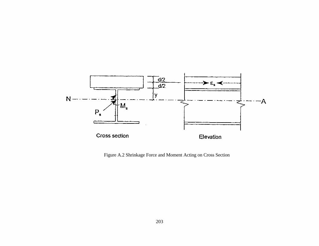
203
Figure A.2 Shrinkage Force and Moment Acting on Cross Section

204
APPENDIX B
LINE GIRDER ANALYSIS
A line girder analysis can provide an effective way to determine deflections and strains
(related to stresses through moments) due to live loading on the bridge.
First, the bridge is reduced to a single girder and deck slab based on an effective width of
the bridge deck. The properties of this section, such as composite (or partial composite) moment
of inertia, area and modulus of elasticity of steel are needed to analyze the bridge.
The total truck load on the bridge is multiplied by the distribution factor (for the interior
girder) to get the point load P acting on the individual girder. The maximum moment (at midspan)
is equivalent to PL/4.
The deflection at midspan is found with PL3/48EI, E (modulus of elasticity) and I (moment
of inertia) can be based on a fully composite or partially composite (cracked) section. Strains are
found from stresses using Mc/I, where M is the moment induced by the point load.

205
APPENDIX C
QUESTIONNAIRE
JOINTLESS BRIDGE DESIGN AND CONSTRUCTION
Your response to the following questions will be used by the Federal Highway Administration todevelop an agenda for a jointless bridge seminar in the fall of 1996. The seminar is beingdeveloped to assist in technology transfer activities and to provide information on successes andfailures. Than you for taking the time to fill out this questionnaire, your answers will provideinsight into the development of sound practices and design specifications for jointless bridges.
State Name: _________________
A. JOINTLESS BRIDGE SEMINAR
1. How many individuals do you plan to send to the upcoming seminar?
2. Do you think that a limited number of individuals from the consultant industry should beinvited to attend the seminar? Yes _____ No _____
3. Would you be willing to share your States current practices/policies and etc. on jointlessbridges at this seminar? Yes _____ No ______If "Yes" what would be the topic and how much time would it take?______________________________________________________________________________________________________________________________________________________________________________________________________________________________________________________(i.e., Successes/Failures, Details that work or Don't Work)
B. GENERAL
1. In your state, how many Jointless Bridges are in service? Integral: _____ Semi-Integral: _____ None: _____
If "None", what are your future plans on Jointless Bridge Construction?____________________________________________________________________________________________________________________________________________________________________________________________________________________________________(If "None", there is no need to fill out the remainder of the questionnaire.)
2. Does your State design and construct Jointless Bridges with:Single Spans: _____ Multiple Spans: _____ or Both: _____

206
3. Number of Jointless Bridges based on superstructure type:Number Max. Span Max. Skew
Steel: _______ _________ _________Prestressed: _______ _________ _________
4. How many Jointless Bridges do you plan to build between 1995-2000?0-5 _____ 6-20 _____ 21-50 _____ 50 or more _____
C. DESIGN AND DETAILS
1. Please attach to this survey, if not previously supplied, any standard details you may have thatrelates to Jointless Bridges (i.e., Bearing Details).
2. Do you have a design procedure for Jointless Bridges?Yes _____ No _____ If Yes, please send a typical design calculation.
3. How do you account for temperature (temperature gradient, thermal expansion and contractionin longitudinal and transverse directions), and creep in your designs?
D. FOUNDATION
1. What is the most common type of foundation used in your State for Jointless Bridges?Bearing Piles _____ Friction Piles _____ Spread Footing _____ Hinged Abutment _____Other_____,Describe_______________________________________________________________________________________________________________________________________
2. What direction do you orient your piles?Weak Axis Parallel to the Centerline of Bearing _____Strong Axis Parallel to the Centerline of Bearing _____Other _____ Please Describe:____________________________________________________________________________________________________________________________________________________________________________________________________________
3. Under what circumstance do you use spread footing as opposed to pile foundation?____________________________________________________________________________________________________________________________________________________________________________________________________________________________________

207
E. ABUTMENT/BACKFILL
1. What measure have you taken to reduce passive earth pressures in Jointless Bridges?____________________________________________________________________________________________________________________________________________________________________________________________________________________________________
2. Have you observed any cracking in abutments/wingwalls caused by bridge movement?________________________________________________________________________________________________________________________________________________________
3. Please provide information on: A. Type of Backfill, B: Gradation, and C: Method and degreeof Compaction.___________________________________________________________________________________________________________________________________________________________________________________________________________________________________________________________________________________________________
F. APPROACH SLAB
1. Please send us a copy of your connection details of an approach slab to a bridge, and approachpavement.
2. Describe any problems you may be having with your approach slabs and how you are dealingwith them? _____________________________________________________________________________________________________________________________________________________________________________________________________________________________________________________________________________________________________
G. RETROFIT (JOINTED TO JOINTLESS)
1. How many Retrofit Projects do you plan to undertake during 1995-2000?0-5 _____ 6- 20 _____ 21-50 _____
2. Please send us the design and construction details for a typical bridge.
3. Has the retrofitting reduced the maintenance problem of leaking expansion joints?____________________________________________________________________________________________________________________________________________________________________________________________________________________________________
4. What modifications do you make in the foundation for retrofitting?

208
____________________________________________________________________________________________________________________________________________________________________________________________________________________________________
5. Approximately, how much does it cost to retrofit a typical joint? ________________________

209
VITA
Jason M. Franco was born on September 21, 1973 in Olean, New York, near his parents’Pennsylvania home, where he grew up and went to school. He completed his Bachelors degree inDecember 1995 at West Virginia University. Jason is currently a Masters degree candidate,scheduled for graduation in May 1999 at West Virginia University.