design and evaluation of pediatric gait rehabilitation robots
TRANSCRIPT

University of Nebraska - LincolnDigitalCommons@University of Nebraska - LincolnMechanical (and Materials) Engineering --Dissertations, Theses, and Student Research
Mechanical & Materials Engineering, Departmentof
12-2016
Design and Evaluation of Pediatric GaitRehabilitation RobotsCale J. StolleUniversity of Nebraska-Lincoln, [email protected]
Follow this and additional works at: http://digitalcommons.unl.edu/mechengdiss
Part of the Biomechanical Engineering Commons
This Article is brought to you for free and open access by the Mechanical & Materials Engineering, Department of at DigitalCommons@University ofNebraska - Lincoln. It has been accepted for inclusion in Mechanical (and Materials) Engineering -- Dissertations, Theses, and Student Research by anauthorized administrator of DigitalCommons@University of Nebraska - Lincoln.
Stolle, Cale J., "Design and Evaluation of Pediatric Gait Rehabilitation Robots" (2016). Mechanical (and Materials) Engineering --Dissertations, Theses, and Student Research. 108.http://digitalcommons.unl.edu/mechengdiss/108

DESIGN AND EVALUATION OF SCALABLE PEDIATRIC GAIT
REHABILITATION ROBOTS
by
Cale J. Stolle
A DISSERTATION
Presented to the Faculty of
The Graduate College at the University of Nebraska
In Partial Fulfillment of Requirements
For the Degree of Doctor of Philosophy
Major: Engineering
(Biomedical Engineering)
Under the Supervision of Professor Carl A. Nelson
Lincoln, Nebraska
December, 2016

DESIGN AND EVALUATION OF SCALABLE PEDIATRIC GAIT
REHABILITATION ROBOTS
Cale Joshua Stolle, Ph.D.
University of Nebraska, 2016
Advisor: Carl A. Nelson
Gait therapy methodologies were studied and analyzed for their potential for
pediatric patients. Using data from heel, metatarsal, and toe trajectories, a nominal gait
trajectory was determined using Fourier transforms for each foot point. These average
trajectories were used as a basis of evaluating each gait therapy mechanism. An existing
gait therapy device (called ICARE) previously designed by researchers, including
engineers at the University of Nebraska-Lincoln, was redesigned to accommodate
pediatric patients. Unlike many existing designs, the pediatric ICARE did not over- or
under-constrain the patient’s leg, allowing for repeated, comfortable, easily-adjusted gait
motions. This design was assessed under clinical testing and deemed to be acceptable.
A gait rehabilitation device was designed to interface with both pediatric and
adult patients and more closely replicate the gait-like metatarsal trajectory compared to
an elliptical machine. To accomplish this task, the nominal gait path was adjusted to
accommodate for rotation about the toe, which generated a new trajectory that was
tangent to itself at the midpoint of the stride. Using knowledge of the biomechanics of the
foot, the gait path was analyzed for its applicability to the general population.
Several trajectory-replication methods were evaluated, and the crank-slider
mechanism was chosen for its superior performance and ability to mimic the gait path

adequately. Adjustments were made to the gait path to further optimize its realization
through the crank-slider mechanism.
Two prototypes were constructed according to the slider-crank mechanism to
replicate the gait path identified. The first prototype, while more accurately tracing the
gait path, showed difficulty in power transmission and excessive cam forces. This
prototype was ultimately rejected. The second prototype was significantly more robust.
However, it lacked several key aspects of the original design that were important to
matching the design goals. Ultimately, the second prototype was recommended for
further work in gait-replication research.

i
DEDICATION
This project was exceptionally difficult to me. My experience lay mostly in
transportation safety and in theoretical research and evaluation of structures. This project
pushed me into an area where I had not been before, and it was both an eye-opening
experience and a challenge. I welcomed it with open arms, but it proved to be difficult.
I’d like to thank my ultimate source of strength and motivation – Jesus Christ. His
wisdom guided my patience and my perseverance through innumerable struggles and
frustrations during this project, and always helped me to keep my eyes on the future.
I’d also like to thank Dr. Carl Nelson. His guidance and support was integral to
both the completion of this project and my efforts in this study. He did not blame me for
the shortcomings of my initial project, and was very understanding about my position and
effort. I don’t think that anyone outside of Dr. Nelson could have pushed me through this
project with such grace and kindness. He has helped me in innumerable ways, and I feel
he will always be a part of my professional future.
I’d like to thank my coworkers who put up with my gigantic mess. The students
working for Dr. Nelson are some of the best coworkers I have ever had, and we shared
many laughs and supported each other through our studies. I’d like to especially thank
Tao Shen, Mohsen Zahiri, Colin and Devin Elley, Gonzalo Garay-Romero, Baoling
Zhao, Kazi Hossain, Saeideh Akbari, and Ross Welch, who stayed with me for most of
my tenure, and put up with not only my massive mess, but also my incessant ramblings
and my jokes and goofiness.
I’d like to thank Dr. Judy Burnfield and Thad Buster for their assistance with this
project, as well as Chase Pfeifer and the rest of the team at the Madonna Rehabilitation

ii
Hospital. Their insight and wisdom provided me with this unique opportunity, and I was
very appreciative of their feedback throughout this entire process.
I would like to thank Candice Schoenherr for her support in some of the tough
times of this project. Her steady resolve was very helpful when things were stressful for
me, and I relied on her strength to finish.
I’d like to thank Ryan Coughlin for his assistance in the construction and design
of the first prototype. His help was extensively useful, and he also served as a motivation
for me to finish the prototype. I’d also like to thank Nathan Borcyk for his assistance with
the final phases of this project including the foot pedals.
I would like to thank my family for their support of me and for always pushing
me to achieve my best. I am truly grateful for their presence in my life. They provided me
with the foundation of what I believe in and the structures of how I perceive the world
and myself. I owe them an eternal debt of gratitude.
Finally, I would like to thank my church family at Cornerstone Christian Church.
They are always reliable, supportive, encouraging, and entertaining. I am proud to be a
part of that group.

iii
TABLE OF CONTENTS
Dedication ............................................................................................................................ i
Table of Contents ............................................................................................................... iii
List of Figures ................................................................................................................... vii
List of Tables ..................................................................................................................... xi
List of Equations ............................................................................................................... xii
Chapter 1 – Introduction ..................................................................................................... 1
Chapter 2 – Literature Review ............................................................................................ 4
2.1 Pediatric Gait .......................................................................................................... 4
2.1.1 Development of Gait ...................................................................................... 4
2.1.2 Comparison of Pediatric and Adult Gait ........................................................ 6
2.1.3 Discussion ...................................................................................................... 8
2.2 Phases of Normal Gait ............................................................................................ 8
2.3 Neurogenic Control of Gait .................................................................................. 11
2.3.1 Chaotic Behavior ......................................................................................... 11
2.3.2 Proprioceptive Behavior .............................................................................. 12
2.3.3 Discussion .................................................................................................... 14
2.4 Gait Therapy Methods .......................................................................................... 15
2.5 Conclusions ........................................................................................................... 20
Chapter 3 – Gait Kinematic Analysis ............................................................................... 21
3.1 The Foot ................................................................................................................ 21
3.2 Stride Trajectory Influences .................................................................................. 22
3.3 Foot Tracking Calculations ................................................................................... 24
3.4 High-Speed Video Analysis .................................................................................. 27
3.5 Winter’s Data ........................................................................................................ 32
3.6 Madonna Adult Treadmill Walking Data ............................................................. 33
3.7 Madonna Child Treadmill Walking Data ............................................................. 37
3.8 Data Comparisons ................................................................................................. 40
3.9 Selection of a Gait Path......................................................................................... 41
Chapter 4 – Gait Path Mathematical Modeling ................................................................ 42
4.1 Fourier Series Modeling of Periodic Gait ............................................................. 42

iv
4.2 Metatarsal Trajectory Modeling ........................................................................... 44
4.2.1 Cartesian Pediatric Gait Modeling ............................................................... 44
4.2.2 Polar Parametrization of Pediatric Data ....................................................... 46
4.2.3 Fourier Series Modeling of Author’s Data .................................................. 53
4.2.4 Fourier Series Modeling of Winter’s Data................................................... 54
4.2.5 Comparison of Mathematical Models .......................................................... 55
4.3 Heel Profile ........................................................................................................... 57
4.4 Foot Angle Modeling ............................................................................................ 61
4.5 Conclusion ............................................................................................................ 64
Chapter 5 – Pediatric Intelligently-Controlled Assistive Rehabilitation Elliptical ........... 65
5.1 Pediatric Considerations ....................................................................................... 65
5.2 ICARE System ...................................................................................................... 66
5.2.1 ICARE Kinematics and Redesign ................................................................ 68
5.3 Crank Design ........................................................................................................ 69
5.4 Screw Selection ..................................................................................................... 72
5.4.1 Screw Calculations....................................................................................... 72
5.4.2 Selected Screw Description ......................................................................... 75
5.5 Simulation Model and Method ............................................................................. 76
5.6 Simulation Results ................................................................................................ 79
5.7 Discussion ............................................................................................................. 82
5.8 Design Issues ........................................................................................................ 83
5.9 Conclusions ........................................................................................................... 84
Chapter 6 – Determination of Gait Replication Method ................................................... 86
6.1 Design Goals ......................................................................................................... 86
6.2 Four-Bar Linkage – Direct Gait Replication ........................................................ 89
6.2.1 Development of Four-Bar Linkage Mathematical Model ........................... 92
6.2.2 Conclusions .................................................................................................. 94
6.3 Pantograph – Direct Gait Replication ................................................................... 94
6.3.1 Pantograph Realization #1 ........................................................................... 95
6.3.2 Pantograph Realization #2 ........................................................................... 97
6.3.3 Assessment of Pantograph Feasibility ......................................................... 98

v
6.4 Foundations of Parametric Gait Modeling ............................................................ 98
6.4.1 Leading Foot Parametric Solution ............................................................... 99
6.4.2 Hip Origin Parametric Solution ................................................................. 100
6.4.3 Parametrization to a Point on the Gait Path ............................................... 101
6.5 Scotch Yoke-Cam – Parametrized Gait Replication ........................................... 104
6.6 Rocker-Cam – Parametric Gait Replication ....................................................... 105
6.7 Conclusions and Chosen Mechanism ................................................................. 106
Chapter 7 – Iteration I ..................................................................................................... 107
7.1 Overall Design .................................................................................................... 107
7.2 Rocker Optimization ........................................................................................... 108
7.2.1 Discussion and Four-Bar Selection ............................................................ 114
7.3 Cam Design ......................................................................................................... 115
7.4 Foot Angle .......................................................................................................... 120
7.5 Full Construction of Iteration I ........................................................................... 124
7.6 Iteration I Performance ....................................................................................... 126
Chapter 8 – Iteration II .................................................................................................... 129
8.1 Design Goals Revisited ....................................................................................... 129
8.2 Complete Design ................................................................................................. 130
8.3 Improved Scaling Mechanism ............................................................................ 131
8.4 Redesigned Rail and Carriage ............................................................................. 132
8.5 Cam Acceleration Limitations ............................................................................ 133
8.6 Removal of Foot Angle Rail ............................................................................... 135
8.7 Motorization ........................................................................................................ 135
8.8 Iteration II Construction ...................................................................................... 138
8.9 Preliminary Performance Evaluation .................................................................. 141
8.10 Conclusions ....................................................................................................... 141
Chapter 9 – Full-Study Discussion and Conclusions ...................................................... 143
9.1 Summary of Research ......................................................................................... 143
9.2 Comparison of Pediatric ICARE and Iteration II Designs.................................. 144
9.3 Adult and Purchasing Recommendations ........................................................... 145
9.4 Scientific Contributions of this Study ................................................................. 146

vi
Chapter 10 – Future Work .............................................................................................. 147
10.1 Improved Gait Trajectory Mathematical Model ............................................... 147
10.2 Pediatric ICARE Improvements ....................................................................... 148
10.3 Pediatric Gait Therapy Device .......................................................................... 149
10.3.1 Double-Axis Pedal Design ....................................................................... 151
10.3.2 Pivoting Plate Pedal ................................................................................. 152
10.3.3 Rotating Pedal .......................................................................................... 153
10.4 Other Gait Rehabilitation Devices .................................................................... 154
10.5 Discussion ......................................................................................................... 154
Chapter 11 – References ................................................................................................. 155
Appendix A – Fourier Series Modeling of Foot Gait Paths............................................ 165
Appendix B – Part Diagrams of Pediatric ICARE Crank ............................................... 188
Appendix C Nonlinear Optimization of Rocker Angular Position Using
MATLAB ............................................................................................................ 193

vii
LIST OF FIGURES
Figure 1. Gait Timing Cycle [30] ....................................................................................... 9
Figure 2. Gait Phases [31] ................................................................................................. 11
Figure 3. Lokomat Used with Adult and Pediatric Patients.............................................. 18
Figure 4. Gait Recovery Effectiveness [79] ...................................................................... 19
Figure 5. Diagram of the Foot [84] ................................................................................... 21
Figure 6. Toe, Metatarsal, and Heel Vectors and Points .................................................. 24
Figure 7. Phases of the Author’s Gait ............................................................................... 28
Figure 8. Author’s Corrected Cartesian Data for Heel, Metatarsal, and Toe ................... 29
Figure 9. Author’s Foot Point Trajectories Relative to Ground ....................................... 30
Figure 10. Author's Normalized Full Foot Trajectories .................................................... 31
Figure 11. Toe Vertical Movement During Stance ........................................................... 32
Figure 12. Winter’s Raw Foot Point Trajectories ............................................................. 32
Figure 13. Winter’s Normalized Full Foot Trajectories ................................................... 33
Figure 14. Madonna Adult Raw Treadmill Metatarsal X vs. Y Data ............................... 34
Figure 15. Points of Interest for Madonna Adult Metatarsal Dataset ............................... 35
Figure 16. Representative Stride for the Madonna Adult ................................................. 37
Figure 17. Madonna Pediatric Metatarsal Raw X vs. Y Data ........................................... 38
Figure 18. Madonna Pediatric Representative Metatarsal Stride Trajectory .................... 39
Figure 19. Comparison of Metatarsal Trajectories ........................................................... 40
Figure 20. Height of Toe at First Peak (Initial Swing) ..................................................... 40
Figure 21. Cartesian Parametrization of Normalized Pediatric Metatarsal
Trajectory .............................................................................................................. 42
Figure 22. Mathematical Model of Normalized Cartesian Gait Coordinates
(ox=2,oy=6) ............................................................................................................ 46
Figure 23. Closed-Loop Trajectory of Cartesian Mathematical Model (ox=2,oy=6) ........ 46
Figure 24. Origin Locations for Analyzing Closed-Loop Polar Parametric
Equations............................................................................................................... 47
Figure 25. Polar Parametrization of Metatarsal: Origin at Centerline Stride ................... 47
Figure 26. Polar Parametrization of Metatarsal: Origin Leading Foot ............................. 48
Figure 27. Polar Parametrization of Metatarsal: Origin Trailing Foot ............................. 48

viii
Figure 28. Polar Parametrization of Metatarsal: Origin at Hip ......................................... 49
Figure 29. Polar Parametrization of Metatarsal: Origin Trailing Hip ............................... 49
Figure 30. Circular Toe Trajectory Modeling [92] ........................................................... 50
Figure 31. Multi-Subject Circular Toe Trajectory Modeling [93] .................................... 51
Figure 32. Mathematical Approximation of Polar Parametrization (ox=2,oy=6) .............. 53
Figure 33. Comparison of Fourier Constants for X and Y Trajectory Coordinates ......... 55
Figure 34. Fourier Series Average Metatarsal Trajectory Parametrization
(ox=8,oy=8) ............................................................................................................ 57
Figure 35. Fourier Series Average Metatarsal Trajectory (ox=8,oy=8) ............................. 57
Figure 36. Parametric Modeling of Pediatric Heel Data (ox=2,oy=3) ............................... 58
Figure 37. Parametric Modeling of Author’s Heel Data (ox=2,oy=3) ............................... 59
Figure 38. Parametric Modeling of Winter's Heel Data (ox=2,oy=3)................................ 59
Figure 39. Fourier Series Average Heel Trajectory Parametrization (ox=8,oy=8) ............ 60
Figure 40. Fourier Series Average Heel Trajectory (ox=8,oy=8) ...................................... 61
Figure 41. Pediatric Foot Angle Data Mathematical Modeling (ox=3) ............................ 62
Figure 42. Author's Foot Angle Data Mathematical Modeling (ox=5) ............................. 62
Figure 43. Winter's Foot Angle Data Mathematical Modeling (ox=4) ............................. 63
Figure 44. Mathematically-Averaged Fourier Series Foot Angle and Datasets
(ox=8) .................................................................................................................... 64
Figure 45. ICARE by SportsArt........................................................................................ 67
Figure 46. ICARE Coupler and Curved Bars ................................................................... 68
Figure 47. Existing and Proposed ICARE Crank Designs ............................................... 70
Figure 48. Foot Pedal Paths for Varying Crank Lengths .................................................. 71
Figure 49. Normalized Foot Pedal Trajectories for Varying Crank Lengths ................... 72
Figure 50. Simple Screw Loading for Screw Selection Calculations ............................... 73
Figure 51. Screw Stress Orientations ................................................................................ 74
Figure 52. Component Labels and Loading Locations ..................................................... 77
Figure 53. Simulated Crank, Bracket, and Screw ............................................................. 77
Figure 54. Shear Planes on Simulated Crank in Lateral Loading Configuration ............. 80
Figure 55. Maximum Stress State During Dynamic Testing ............................................ 82
Figure 56. Pediatric ICARE Final Design ........................................................................ 84

ix
Figure 57. Four-Bar Mechanical Isomers ......................................................................... 89
Figure 58. Sample Coupler Trajectories [106] ................................................................. 92
Figure 59. Single Pantograph Frame ................................................................................ 95
Figure 60. Pantograph Path-Tracing Mechanism: Design 1 ............................................. 96
Figure 61. Pantograph Path-Tracing Mechanism: Design 2 ............................................. 97
Figure 62. Sample Radial Parametrization of Metatarsal Trajectory ............................... 99
Figure 63. Scalable Device with Polar Origin at Hip ..................................................... 101
Figure 64. Projected Foot Path with Minimized Trajectory Height at Center Stride ..... 102
Figure 65. Raw Radial and Angular Traces of Mathematically Predicted Point ............ 103
Figure 66. Smoothed Mathematically-Predicted Gait Path Radial Parametrization ....... 103
Figure 67. Scotch Yoke Realization of Parametric Modeling ........................................ 104
Figure 68. Rocker-Cam Parametric Gait Replication ..................................................... 105
Figure 69. Proposed Mechanism Control Systems ......................................................... 108
Figure 70. Initial Four-Bar Linkage Configuration for Analysis .................................... 109
Figure 71. Nonlinear Optimization Comparison of Four-Bar Rocker Angles................ 113
Figure 72. Nonlinear Optimization Configuration I ....................................................... 113
Figure 73. Nonlinear Optimization Configuration II ...................................................... 114
Figure 74. Timing Lag for Chosen Four-Bar Linkage .................................................... 115
Figure 75. Time-Adjusted Cam Height Profile............................................................... 116
Figure 76. Cam Acceleration Profile .............................................................................. 117
Figure 77. Cam Displacement Profile ............................................................................. 118
Figure 78. Iteration I Cam Shape .................................................................................... 119
Figure 79. Mechanical vs. Desired Gait Trajectories ..................................................... 119
Figure 80. Foot Pedal Model .......................................................................................... 120
Figure 81. Ideal Heel Lift Height Profile ........................................................................ 121
Figure 82. Acceleration Comparison between Ideal and Acceleration-Limited
Profiles ................................................................................................................ 122
Figure 83. Heel Lift Displacement Comparison ............................................................. 122
Figure 84. Foot Angle Cam Shape .................................................................................. 123
Figure 85. Mechanical vs. Desired Foot Angle Comparison .......................................... 124
Figure 86. Iteration I Design: Front Right View............................................................. 124

x
Figure 87. Iteration I Design: Front Left View ............................................................... 125
Figure 88. Iteration I Design: Top View ......................................................................... 125
Figure 89. Iteration I Design: Rear Left View ................................................................ 126
Figure 90. Conceptual Design of Iteration II .................................................................. 130
Figure 91. Component Model of Iteration II .................................................................. 131
Figure 92. Off-The-Shelf Rail and Linear Motion Carriage ........................................... 132
Figure 93. Cam Acceleration Comparison ...................................................................... 134
Figure 94. Rail Angular Displacement Comparison ....................................................... 134
Figure 95. Initial Power Transmission Configuration .................................................... 136
Figure 96. Chain-Tensioned Power Transmission Diagram ........................................... 137
Figure 97. Dual-Chain Power Transmission System ...................................................... 138
Figure 98. As-Designed Iteration II Assembly ............................................................... 139
Figure 99. Assembled Iteration II with New Foot Pedal ................................................ 140
Figure 100. Base Configuration for Proposed Iteration III Gait Mechanism ................. 150
Figure 101. Dual-Axis Pivoting Foot Pedal Design ....................................................... 151
Figure 102. Pivoting and Locking Foot Pedal Design .................................................... 152
Figure 103. Rotating Foot Pedal Design ......................................................................... 153

xi
LIST OF TABLES
Table 1 Average Process for Learning Gait [6] .................................................................. 5
Table 2. Gait Phases [31] .................................................................................................. 10
Table 3. Summary of Madonna Adult Stride Analysis ..................................................... 36
Table 4. Madonna Pediatric Metatarsal Data Summary ................................................... 39
Table 5. Fourier Series Constants for Pediatric Cartesian Parametrization ...................... 45
Table 6. Fourier Series Constants for Pediatric Polar Parametrization ............................ 52
Table 7. Fourier Series Constants for Cartesian Modeling of Author's Data ................... 54
Table 8. Fourier Series Constants for Cartesian Parametrization of Winter’s Data ......... 54
Table 9. Fourier Series Average Metatarsal am and bn Constants ..................................... 56
Table 10. Fourier Series Average Heel am and bn Terms .................................................. 60
Table 11. Average Fourier Series Constants for Foot Angle Modeling ........................... 63
Table 12. 3/8-12 ACME Threaded Screw Parameters...................................................... 75
Table 13. Maximum Observed Von Mises Stresses in Simulated Crank – Original
Mesh ...................................................................................................................... 80
Table 14. Maximum Observed Von Mises Stresses in Simulated Crank – Reduced
Mesh ...................................................................................................................... 81
Table 15. Grashof Existence Condition for Four-Bar Linkages ....................................... 90
Table 16. Iteration I Performance vs. Design Goals ....................................................... 128
Table 17. Iteration II Performance vs. Design Goals ...................................................... 142
Table 18. Design Goal Comparison Between Pediatric ICARE and Iteration II............ 144

xii
LIST OF EQUATIONS
Equation 3-1. Origin Coordinate Shift .............................................................................. 25
Equation 3-2. Adjustment of Trajectories to Hip Position ............................................... 25
Equation 3-3. Normalized Trajectory Vector ................................................................... 27
Equation 3-4. Summation of Deviations ........................................................................... 38
Equation 4-1. Fourier Series Equation .............................................................................. 43
Equation 4-2. Normalized Fourier Series Equation .......................................................... 43
Equation 4-3. First Term in Fourier Infinite Series .......................................................... 43
Equation 4-4. Concurrent Terms in Fourier Infinite Series .............................................. 44
Equation 4-5. Cartesian Parametrization Using Fourier Series ........................................ 44
Equation 4-6. R2 Calculation for Fourier Regression ....................................................... 45
Equation 4-7. Radial Parametrization Using Fourier Series ............................................. 52
Equation 5-1. Screw Axial Stress ..................................................................................... 72
Equation 5-2. Screw Lateral and Shear Forces [98] ......................................................... 73
Equation 5-3. Torque Required To Turn Screw Against Applied Load [98] ................... 74
Equation 5-4. Fatigue Safety Factor Determination ......................................................... 74
Equation 5-5. Von Mises Stress Calculation [98] ............................................................. 76
Equation 6-1. Parametric Equations of Four-Bar Linkage Positions ................................ 92
Equation 6-2. Freudenstein’s Equation [107] ................................................................... 93
Equation 6-3. Foot Point Gait Path Determination ......................................................... 102
Equation 7-1. Rocker Angle (Derived from Freudenstein’s Equation) .......................... 110
Equation 7-2. Optimization Function (Least-Squares Error) .......................................... 111
Equation 7-3. Iterative Equation for Optimization Problem ........................................... 112
Equation 7-4. Minimizing Direction Vector for Steepest Descent ................................. 112
Equation 7-5. Foot Angle Relationship with Rail Lift .................................................... 120

1
CHAPTER 1 – INTRODUCTION
Since the dawn of humanity, walking has been an integral aspect of life. The
ability to walk defines the growth of children, the strength of adults, and the decline of
health in the elderly. The inability to effectively ambulate comes with a host of physical,
psychological, and social implications that are detrimental to the overall well-being of a
human. In short, walking is one of the major indicators of human health.
The main purpose of perambulation is mobility. In general, mobility is defined as
the capacity to move through physical space, although true mobility spans much farther
than this simple definition. Schwanen and Ziegler suggest that mobility, independence,
and well-being are all interdependent and complicated mechanisms that complement each
other, and can’t be undervalued for their importance [1]. According to Schwanen and
Ziegler,
[F]or those whose embodied capacities have diminished over time
mobility, independence and wellbeing can become linked up in a
downward spiral (p. 724).
The impact of mobility on physical and psychological health is profound.
Immobility and reduced mobility are linked to a long list of physical health problems
spanning across every major organ system [2]. Some of the complications are increased
risks for blood clots, indigestion, osteoporosis, changes in hormone balance, bladder
infections, pressure ulcers, atrophied muscles, difficulty expanding lungs fully, weakened
coughs, and low back pain. Psychologically, immobility can cause depression, anxiety,
apathy, mood swings, feelings of helplessness, loss of normal sleep cycles, and delirium.

2
According to the U.S. Census, 30.6 million American adults and teenagers
experience difficulty in perambulation, including walking or climbing stairs [3].
Correspondingly, about 3.6 million people use a wheelchair and 11.6 million people use
another form of assistance when walking, such as a cane or walker. The census survey
also asked about information on difficulty moving large objects (such as a chair),
reaching the top shelf, and standing for long periods of time. The inability to effectively
perambulate affects more than simply the ability to move from one location to another.
Gait therapy involves a series of guided tasks facilitated by a therapist in which an
individual moves through the motions of walking, often with significant assistance. Gait
therapy is useful for many purposes. For one, gait therapy can be used to teach the correct
leg movements involved in walking. However, it can also be used with individuals who
are unable to walk to provide them with valuable exercise to increase their health. The
prevalence of individuals with gait-related disabilities and ambulatory issues adds to the
need for reliable, cost-effective gait therapy treatment and exercise.
Gait therapy is especially important for children. According to the U.S. Health
and Human Services Advisory Committee, children’s muscular, skeletal, and
cardiovascular health all show marked improvement with increased physical exercise [4].
Aside from physical benefits, learning how to walk is integral to the development of
psychological independence. Between the ages of one and three, children begin to use
their newfound walking ability as a way of expressing and exploring their own capability.
Erikson [5] theorized that inhibitions in this stage, such as repression of walking
capability, would tend to incur self-doubt and self-esteem problems in children that
would last for years to come.

3
Because of this, gait therapy is needed for children. However, many of the gait
therapy methods that are used for children right now are either clinician-intensive or
expensive. This is an issue when it comes to rural or smaller rehabilitation facilities,
hospitals, or home health centers. As such, there exists a need for inexpensive, easy-to-
use, effective pediatric gait therapy equipment.
Realistically, there are no gait therapy mechanisms that accurately trace gait
trajectories every cycle. However, it is currently unknown what effect gait mechanisms
have on therapy as their trajectory becomes more gait-like. One of the goals of this
research is to develop a gait-like machine and compare to existing rehabilitation
technologies. Using the new machine, it will be possible to determine whether the
cyclical, repetitive nature of current gait rehabilitation is the driving force behind gait
therapy or if the therapy effectiveness is correlated to trajectory accuracy.

4
CHAPTER 2 – LITERATURE REVIEW
The goal of pediatric gait therapy is to guide the legs muscles through a gait-like
motion for both physical exercise and for teaching muscular movements involved in
walking. This is particularly necessary following surgery, illness, accidents, birth defects,
and other factors that cause temporary immobility in children. Since walking is the major
form of exercise for humans, this therapy is necessary to improve the health and future of
children. However, to understand how therapy works, it is necessary to understand the
walking motions of children first.
2.1 Pediatric Gait
2.1.1 Development of Gait
Normally, children develop walking skills in a predictable manner, reaching
landmark achievements on a fairly rigid timeline. According to Christopher Heffner,
“most agree that these abilities are genetically preprogrammed within all infants” [6].
Heffner presented his timeline for when normal gait should occur and the
sequential order of learning stages [6]. The learning progression is shown in Table 1.

5
Table 1 Average Process for Learning Gait [6]
Approximate Age Skill Mastery
2 months Able to lift head up without assistance
3 months Able to roll over
4 months Can sit propped up without falling over
6 months Able to sit up without support
7 months Begins to stand while holding onto things for support
9 months Can begin to walk, still using support
10 months Is momentarily able to stand without support
11 months Can stand alone with more confidence
12 months Begins walking alone without support
14 months Can walk backward without support
17 months Can walk up steps with little or no support
18 months Able to manipulate objects with feet while walking (such as
kicking a ball)
The learning progression of how infants come to walk takes many months. During
this process, they are increasing their muscle strength, improving their balance, and
learning motor control of their limbs for successful gait. Each step (such as learning to
crawl and learning to stand with assistance) is developing one of these three areas that are
pertinent to the next step.
The factors affecting the development of normal gait vary with each child
depending on both their genetic makeup and their environment. Adolph et al. postulated
that the three major developmental factors were body dimensions, neural pathways, and
walking experience [7]. An experiment conducted by cross-evaluating infants,
kindergarteners, and adults showed that there were positive correlations between
normality of gait patterns and each of these factors. With body dimensions changing until

6
the completion of puberty, this infers that gait development is not fully established until
adulthood. In order to design for children, it is then important to focus on the similarities
and controllable factors, as opposed to the variations existing through natural
development.
Early in a child’s development, children display the cyclical leg motions where
each leg moves identically, phase-shifted by half a cycle [8-9]. Joint flexion and angles
are very similar between infant kicking and adult walking, and much of the leg
movement timing is dependent on the weight of the child’s leg [10-11].
Some researchers have noted that gait maturation continues until after the age of
14 [12-15]. Variations, growth, and strengthening of the musculoskeletal structure is
attributed to the variation of stride lengths and timing noted in that maturation process.
Even though the stride length and timing matures into puberty, the stochastic timing
difference in strides is close to the adult value beginning at age 6 [16].
2.1.2 Comparison of Pediatric and Adult Gait
Comparing the gait trajectories for children and adults shows one major
difference: the size of the adult stride length is significantly larger than the pediatric
stride length. In order to make a valid comparison between the child and the adult, the
gait trajectories must be normalized. Hof suggested that there were several variables
available to normalize by using the human body [17]. Specifically related to gait, the
normalization factor would be the leg length. Dimensionless data plotted for children
ages 1 to 7 shows a strong correlation between the leg length and the stride length,
meaning that the stride length could be used as an acceptable normalization factor [18].
Normalization allows for direct comparison regardless of size.

7
Sutherland noted that the gait of children appeared to “mature” to match the
characteristics of adult ambulation [18]. Dimensionless data plotted for children ages 1 to
7 shows a strong correlation between the leg length and stride length. Further analysis
shows that there is a maturation of stride length in relation to age. Similar maturation is
noted in joint angles, muscular force data, oxygen consumption rate, and pelvic
span/ankle spread ratio.
Ganley and Powers tested to see if pediatric gait was statistically different from
adult gait motion [19]. A study group of 7-year-olds had a much smaller stride length and
higher cadence, but very similar walking velocity. Data also proved that ankle power and
ankle moments were significantly smaller in children than in adults. Other gait kinetics
mimicked that of adult data. Studies conducted by Chester et al. determined significant
difference in ankle plantarflexor moments, sagittal knee moments, sagittal hip moments,
frontal hip moments, and hip power [20-21]. Slight angle differences were noted for each
of these joints as well, but it was not deemed significant enough to claim that pediatric
gait was dissimilar from adult gait.
In one study involving 28 children, knee and ankle flexion and heel strike
occurred normally by age 40 months, implying that adult gait patterns may be present
earlier in child development than previously thought [22]. Metatarsal trajectory relative to
the trunk appears to be similar to adult metatarsal trajectory as early as age 3 [18].
Dimensionless data compared between children ages 5 to 12 showed that there was very
little difference in stride parameters throughout the age range [23]. The general
consensus, however, is that child gait patterns reliably reach full maturity at or before age
7 [7, 19, 24-29].

8
2.1.3 Discussion
Immature, unreliable gait trajectories are noted in young children, and continue
into adolescence. Thus, measuring gait data of young children is sporadic and does not
show significant convergence. However, despite the variation of data, normal pediatric
strides have similar shape and body position to adult strides beginning at age 3, and are
fully similar by age 7, although stride length and time change. As a result, pediatric gait
therapy should aim to reproduce normal adult gait. This will encourage proper foot angles
and metatarsal trajectory.
2.2 Phases of Normal Gait
In normal gait, both legs are identical, and neither offers any physical difference
from the other. Thus, during normal gait, the motions are both cyclical and symmetric
[30]. The limb cycle involves two double-support phases (where both legs are on the
ground) and two single-support phases (where one leg is in the air). The body assumes
different distinct positions during the gait phase, which can be approximated by the time
the time they occur relative to the length of the stride time. A timed gait cycle is shown in
Figure 1. Note that this image assumes that the stride starts and ends on initial contact of
the shaded leg.

9
Figure 1. Gait Timing Cycle [30]
Perry separated the gait cycle into 8 distinct phases [31]. Each phase was marked
by joint rotation values of interest, as well as active constraints on the foot at the time.
The phases are explained in Table 2 and shown graphically in Figure 2.

10
Table 2. Gait Phases [31]
Phase of Gait Description
Initial Contact Moment when the foot first strikes the ground.
Loading
Response
Initial double support period when the limb begins to accept
weight. At the end of this phase, the opposite limb experiences
toe-off.
Mid-Stance
First phase of the single-support when the body advances over the
stance limb and weight is transferred from the rear of the foot
towards the front of the foot.
Terminal Stance Last phase of the single-support which ends when the opposite
limb experiences first contact.
Pre-Swing
Final double-support period when the knee experiences rapid
flexion in preparation for swing and when the weight is shifted to
the opposite limb. This phase ends in toe-off.
Initial Swing
The first third of the swing period where the maximum knee
flexion occurs. This phase ends when the heel of the swinging
foot passes the heel of the opposite limb.
Mid-Swing
Middle third of the swing period where maximum hip flexion
occurs. At the end of this phase, the tibia is vertical,
perpendicular to the ground surface.
Terminal Swing
Last third of the swing period where the final knee extension
achieves maximum step length, and the limb is put in position to
accept weight transfer again. This phase ends in initial contact.

11
Figure 2. Gait Phases [31]
2.3 Neurogenic Control of Gait
2.3.1 Chaotic Behavior
When the trajectory of each point on the foot is measured and traced, they show
similar form with other strides from the same individual. However, they do not share
identical cadence and shape, despite the lack of features in the terrain. The variation
noted between strides of the same individual has been deemed chaotic due to its random
variation of timing and shape.
12
According to Buzzi et al., the nonlinear dynamics observed during gait exist to
assist the body in overcoming obstacles during a normal gait cycle [32]. These seemingly
random variances in stride length, timing, and foot path have been attributed to white
noise, but show a distinct pattern when each stride is viewed sequentially, indicating that
there is a nonlinear pattern affecting the stride variation [33]. This variation displays a
fractal pattern, and is intrinsically healthy to the locomotion of an individual [34].
One of the reasons why chaos is important to the gait pattern is that chaotic
systems have the ability to adjust to random inputs much more easily [35]. In one
perspective, the neuromuscular control of the legs needs to be chaotic in order to
seamlessly transition from normal gait to stair climbing to object avoidance, etc. Having
a set, established, exact gait path would make slight deviations unnatural and gross
deviations challenging, while the chaotic control of gait leads to significantly more fluid
and improved gait transitions, adjustments, and initiations [36-37].
2.3.2 Proprioceptive Behavior
Proprioception is clinically defined as “sensory information that contributes to the
sense of position of self and movement” [38]. It is a complex, multi-sensor input that
involves both afferent and efferent nervous signals and feedback. Proprioception is an
integral part of the motor feedback system, and actively contributes to acuity in fine
muscular movements.
Proprioceptive training requires continuous motion, and as such, this may explain
some of the successes noted by existing gait therapy methods. As stated by Aman et al.,
[I]t needs to be considered that proprioception is closely linked to
movement. Unlike senses such as audition, where, for example, pitch

13
perception can be trained in the absence of limb or body movement,
proprioception requires movement. Thus, when evaluating the
effectiveness of an intervention to improve proprioception, it may be
difficult to isolate the sensory from a motor aspect of training. In fact, one
can argue that any form of motor learning is associated with
proprioceptive processing and thus may train proprioception [39]
According to Miller, proprioception is best practiced through unbalanced,
dynamic movements and teaching the body rapid adjustment to off-center inputs [40].
This is only one type of proprioceptive training, though. Aman et al. classified different
types of proprioception, including passive movement training (focusing on the motion of
only one joint), somatosensation stimulation (vibration of body segments),
somatosensory discrimination (distinguishing of segment rotations and speeds through
contact), and combined / multi-system training (involving multiples of these training
techniques). While Aman et al. conclude that proprioceptive training is not well-defined,
it is noted that there is conclusive evidence that forms of proprioceptive training are
effective rehabilitation methods. This infers that there may not be a singular optimal
solution to proprioceptive training.
A study was conducted based on a stroke patient where everyday activities were
evaluated as therapeutic devices [41]. Results of this study recommend that stroke
patients need to focus on proprioceptive-training tasks to rehabilitate above simply
moving through motions. This was further evaluated in a study determining the effect of
proprioceptors in the gait cycle. Researchers determined that the knee and hip joint angles
during gait were strongly tied to a person’s perception of their foot’s location [42].
Proprioception is integral to protecting the lower limb during gait because the body

14
naturally attempts to minimize contact forces, choosing a gait path that prevents large
impact loading on heel strike. Impact and pressure loading were found to assist in
proprioceptive training, and inhibition of joint movement was found to also inhibit
proprioceptive learning [43]. This indicates that proprioceptors may have a significant
role in determining the gait movements, and also that proprioceptive failure may cause
injury and gait abnormalities.
Other studies into therapeutic proprioceptive training have verified that
proprioceptive training is beneficial to gait motions, rehabilitations, and overall health
[44-47]. It has been noted, however, that proprioceptive training only teaches correct
form during walking, but does not improve timing [48].
2.3.3 Discussion
The proprioceptive and chaotic behaviors noted in gait share one commonality:
both methods show that the foot is guided through a path to avoid excessive loading of
the foot, as is seen in kicking, tripping, or stomping. Also, the biomechanical feedback
from normal gait is shown to assist in recurring normal gait paths, as expected in a
proprioceptive system [49]. This infers that there may be a correlation between the
proprioception of the foot and the chaotic nature of gait. This also implies a
success/failure condition in gait, one where premature or unexpected foot contact is
deemed unacceptable. During the swing phase of a gait cycle, three points on the foot risk
contact with the ground or object: (1) the toe following toe-off, (2) the metatarsal at
midswing, and (3) the heel at terminal swing. If contact occurs between the foot and the
ground during any of those phases, the stride can be considered a failure.

15
The success/failure condition imposed by the proprioceptive and chaotic behavior
of gait implies that successful therapy must prevent premature foot contact during gait by
retraining the proprioception of the body to resume normal, fractal-like chaotic gait
patterns. However, other factors are integral to therapy, such as overextension, prevention
of muscular damage or excessive joint loading, and timing.
2.4 Gait Therapy Methods
The type of gait therapy available to individuals is dependent on their level of
muscular strength. A patient with high muscular strength and control would be able to
participate in most types of therapy, whereas patients with little to no muscular strength
or control are very limited in their options.
The simplest form of therapy involves physical therapists manually assisting a
patient’s feet through a gait-like trajectory. Patients often have motive-assisting devices,
such as walkers, parallel bars, or a body weight support system. This therapy method has
proven effective [50]. However, this method can require specialized training, a
multiplicity of therapists, and significant exertion [51].
Body weight-supported treadmill training is less intensive and expensive,
assisting clinicians in powering the foot through a gait-like trajectory without requiring
the patient to move. Treadmill training has shown to be effective for patients with a
minimal amount of strength [52,53], but still requires significant effort from the therapist
to guide metatarsal trajectories. One study showed that that the mean difference between
treadmill walking and overground walking was very small, beating out both cycling and
elliptical therapy methods [54].

16
Robotic-assisted gait therapy involves the use of automated actuation to assist in
propelling the patient’s foot through a gait-like trajectory. The idea is that fixing hip,
knee, and/or ankle flexion can help teach the foot to track a more gait-like trajectory. A
variety of types of robotic orthoses have been developed [55-59], each stating that they
have improved joint angles during gait. A study conducted using robotic gait orthoses on
pediatric cerebral palsy patients with poor gross motor control showed improvement after
robotic gait training [60]. Also, robotic systems have shown to better rehabilitate natural
gait motions than some elliptical devices due to their more accurate full-foot angle and
trajectory [61]. These devices tend to be expensive, and, as stated earlier, constrain the
joint and limit the ability to improve proprioception. This might explain why some
research indicates that robotic-assisted gait treatment does not show as much
improvement as therapist-assisted gait treatment [62]. However, some newer devices are
in development that are both cheaper and simpler [63-66].
Motorized foot-propelling devices, such as elliptical machines, guide the foot
through a looping trajectory. Elliptical machines require less effort from the therapist
than does treadmill training, making this an easier option for clinics seeing many patients
and for people with little muscular strength. Elliptical machines also tend to be easier to
operate and cheaper than robotic systems. Kinematic analyses of elliptical devices show
that they do assist in effective gait rehabilitation [67-72]. However, as stated earlier, some
elliptical devices have shown poorer performance than robotic or treadmill training [60],
and their motion does not match normal gait [54].
Gait rehabilitation techniques have been developed by researchers using
treadmills with body weight support systems [51] and robot-assisted driven-gait orthoses

17
[74]. The Lokomat combines robotic gait orthoses with exercise equipment to improve
the quality of training while reducing the work load required from the clinician [75-77].
The Lokomat is adjustable to function with both adult and pediatric patients. However,
the cost makes the Lokomat infeasible for many small rehabilitation clinics and home
health centers [75]. The Lokomat is shown with both adult and pediatric patients in
Figure 3.

18
Figure 3. Lokomat Used with Adult and Pediatric Patients
According to Langhorne et al., following a stroke, physically-intense therapy
appears to be the most effective form of treatment, offering the most advantage over a
placebo therapy session [79]. Several therapy methods are compared for effectiveness in
Figure 4, which offers standard means and deviations (SMD) for objectively-rated
therapy methods based on existing literature and data. According to the chart, the most
effective forms of therapy involve a cardiovascular element, proper proprioception, and
repetition of movements with mechanical assistance. While stroke patients are not fully
representative of every patient needing gait therapy, this chart still provides a foundation
for understanding effectiveness of individual treatment methods. It should be noted that
the treadmill training received positive scores during this study. However, despite its
prevalence in rehabilitation, it was not as effective as other, more controlled methods that
train proprioception and foot positioning.

19
Figure 4. Gait Recovery Effectiveness [79]
One device which addresses some of these concerns is the Intelligently Controlled
Assistive Rehabilitation Elliptical (ICARE) system, developed by researchers at
Madonna Rehabilitation Hospital and the University of Nebraska [80,81]. The ICARE is
a relatively low-cost, ergonomic, effective gait rehabilitation device for adults. The
device is a modified, motorized elliptical machine that has been designed to push a

20
patient’s feet through an approximation of gait-like motion. Unlike many other
rehabilitation devices, the ICARE was designed so that little muscular strength is
required to operate the machine. However, if the patient has sufficient muscular strength,
they are able to drive the machine themselves without requiring the motor [82]. Studies
have shown that this device effectively meets many of the requirements for gait
rehabilitation. While the device emulates the kinematic and EMG demands of adult gait
[83], the foot path is elliptical, which is not gait-like in shape or cadence.
The success of the ICARE follows the discussion from Section 2.3.2. While some
gait therapy devices have sought to control joint angular motions and specific body
postures during gait, the body needs to relearn the proprioceptive positioning needed for
the foot to walk, as the ICARE has done. When designing a new gait rehabilitation
device, it need not be intensive in its limbic control, but it needs to teach the foot
proprioception.
2.5 Conclusions
Designing a device that facilitates rehabilitation for both adults and children,
accommodating a broad range of stride lengths, is going to require uniformly scaling the
path, which is identical in shape when normalized against the stride length. Initial efforts
to construct a pediatric gait therapy machine will begin with the ICARE system. The
ICARE has proven to be effective for adult therapy, it is expected to have similar results
with pediatric patients. However, a secondary study will be performed to understand the
gait path. It is believed that close approximation of the gait path will provide adequate
proprioceptive training to better improve gait therapy methods. This will be pursued in a
new, novel invention.

21
CHAPTER 3 – GAIT KINEMATIC ANALYSIS
According to the results noted in Section 2.1.2, it is difficult to capture the full
scale of a pediatric stride. While adult data is significantly more consistent, pediatric data
shows large variances in trajectory length and timing. Thus, an effort was made to
understand both the adult gait and the pediatric gait.
3.1 The Foot
The foot is comprised of 26 different bones – 14 phalangeal bones (comprising
the toes), 5 metatarsal bones (comprising the ball of the foot and the forefoot), and 7
tarsal bones (comprising the midfoot and hindfoot). A diagram of the human foot is
shown in Figure 5.
Figure 5. Diagram of the Foot [84]
Each of the joints in the foot fills a specific purpose. Some of those joints (such as
the subtalar joint between the talus and the calcaneus) provide vertical support for the

22
tibia and allow for mild lateral movement for uneven ground [85]. While there is some
movement out of the first and second metatarsal, the gross motion of the metatarsals and
tarsals are effectively zero, and these are often modeled as being rigid links for
simplicity. The metatarsal-phalangeal joint provides a significant rotation of the
phalanges, and because of that, many foot models treat the phalanges as another rigid
link. The metatarsal-phalangeal joint axis provides the major flexure of the foot during
gait.
During gait, the foot traces a path in the sagittal plane. While there is some lateral
movement during gait, the movement is relatively insignificant and varies between
individuals. Thus, only the sagittal plane is measured when reviewing the each foot
point’s trajectory in this work. Three distinct points on the foot exist in the sagittal plane,
which are helpful in defining the foot position: the heel (posterior location of the foot),
the first metatarsal (location of the metatarsal-phalangeal joint axis) and the big toe
(anterior location on the foot).
3.2 Stride Trajectory Influences
The gait stride trajectory differs between two individuals for many reasons.
Differences in kinematics can occur based on varying force requirements in limbs and
proprioceptive learning processes, among other factors. However, the effect of these
influences on the trajectory of foot points during gait are not well-understood. Some
studies have been conducted on factors like heel heights of females [86-90], but these
studies don’t focus specifically on gait trajectory.
Influences that may affect the measured foot point trajectories during gait:
Shoe compliance (Sole material, metatarsal flexure resistance)

23
Shoe dimensions (Sole height profile, length of shoe posterior and anterior
to the metatarsal)
Ground compliance (Rigid vs. soft)
Clothing (Compliance, weight, cover)
Foot dimensions (Length posterior to metatarsal, length anterior of
metatarsal, height of ankle, foot width)
Leg dimensions (Tibial length, femoral length, distance between hip
joints)
Joint nonlinearities (Knee rotation joint trajectory, hip vertical motion,
ankle compression)
Gender
Limb Masses (Mass of toe, mass of foot, calf weight profile, thigh weight
profile)
Muscular strength (foot, ankle, calf, thigh, buttock, dorsal)
Gait hysteresis
Neurological factors (Perceived obstacles, balance, proprioception)
Age
Gait experience (Time since last gait injury, total amount of walking)
Compensating and studying each of these factors would be a monumental task. As
such, this research will focus on methods of gathering and comparing data, which will
hopefully establish a foundation for future research in these areas and their effect on foot
point trajectories during gait.
24
3.3 Foot Tracking Calculations
When tracking foot data, vectors are collected relative to a fixed coordinate
system. Often, the origin is a static location in the room that is arbitrarily chosen. Vectors
showing the heel, metatarsal, and toe vectors and points, as well as the segmented model
of the foot, are shown in Figure 6.
Figure 6. Toe, Metatarsal, and Heel Vectors and Points
Several inaccuracies exist in measuring the foot locations. The heel, metatarsal,
and toe vectors (labeled in Figure 6 as �̅�, �̅�, and �̅�, respectively) are vectors measured
from the arbitrary origin to the point on the heel, metatarsal, or toe. However, shifting of
the skin, movement of the point relative to the body, and an inability to directly measure
the bone of the participant prevents these points from precisely representing the skeletal
motions.
Ideally, the Y axis of the arbitrary origin is aligned with the direction of gravity.
However, a coordinate system rotation may be necessary. For the metatarsal data, the foot
travels along a flat trajectory during the stance phase. This provides a good point of
reference to create a representative ground line. The angle between the ground line and
the X axis is the negative of the coordinate axis rotation angle δ.

25
In order to obtain the new position vectors in the shifted coordinate system X’-Y’,
the original vector must be multiplied by the rotation matrix R and, if desired, the origin
can be shifted to a new location. This shift is represented by Equation 3-1.
�̅�′ = �̿� ∗ (�̅� − 𝐶̅)
Equation 3-1. Origin Coordinate Shift
where �̅�′ is the rotated position vector (with the foot travelling flat along the X’ axis
during stance) and �̅� is the original position vector of the point. The rotation matrix 𝑅 =
[cos 𝛿 sin 𝛿
− sin 𝛿 cos 𝛿] is used to shift the coordinates. The vector 𝐶̅ is the vector from the old
origin to the new origin using the unrotated coordinate system. It is important to use this
shift for the toe, metatarsal, heel, and hip datasets.
Joints in the leg and foot have nearly identical angular paths during repeated
normal gait. This means that the foot position traces roughly the same trajectory relative
to the hip. Regardless of whether the data was collected from participants on a treadmill
or overground walking, the metatarsal, toe, and heel position vectors need to be adjusted
by the movement of the hip. The hip rises and falls during each stride due to the rotation
of the hip bones about the base of the spine. Compensation for this motion does not
provide consistent results. Thus, only the longitudinal travel of the hip is adjusted. The
X’-position of the hip is forced to be zero so that the hip only travels along the Y’ axis.
The metatarsal, heel, and toe values must be adjusted accordingly. This is represented by
Equation 3-2.
{�̅�′}𝐴𝑑𝑗 = {�̅�′} − {𝐻𝑖𝑝𝑥′, 0}
Equation 3-2. Adjustment of Trajectories to Hip Position

26
where {�̅�′}𝐴𝑑𝑗 is the dataset of all vectors �̅�′ adjusted for the longitudinal movement of
the hip. {𝐻𝑖𝑝𝑥′, 0} is the dataset of all hip X positions. This equation can only be true if
hip measurements were made simultaneously with the toe, metatarsal, and heel
measurements.
After this adjustment, the metatarsal, heel, and toe trajectories show periodic
trends, and can generate closed-loop trajectories starting and ending at mid-stance. It
should be noted that due to periodic chaotic trends (noted in Section 2.3.1), the trajectory
of each point on the foot may not form a closed loop when starting or ending from any
other location in stride. Also, there may be some error in the datasets present where the
loop is not closed and the two ends do not appear to connect. This error is due to
measurement error, often because of the out-of-plane movement of the foot during gait
where the footfall of one foot lies lateral to the footfall of the former step. This error is
small relative to the height of the trajectories.
Each stride needs to be separated from the dataset so they can be analyzed
individually. Each stride has a different path, and does not coincide with the previous
path. Thus, the best location to measure the start and end of the stride is when the foot
crosses the Y’ axis while in stance, marking the midstance phase. The foot is completely
flat, and remains flat and in contact with the ground for much of the stance phase. This
means that all of the points on the foot undergo only longitudinal travel relative to the
hip, making it easier to splice together the ends of the datasets. If any dataset is seen
where one of these points is not in contact with the ground or only traveling
longitudinally at the midstance location, it must be thrown out as it is not normal gait.

27
As discussed in Chapter 2, the normalized gait path from a child of at least age 7
is similar to the trajectory of the foot of an adult during normal gait. To normalize the
trajectory, the trajectory of each point on the foot must be divided by the length of the hip
travel during one stride, and can be determined by measuring the {𝐻𝑖𝑝𝑥′, 0} vector along
one full stride. A simpler method for normalizing uses the length of the metatarsal travel
during one stride, measuring the foremost X’ position to the rearmost X’ position. Using
the approximate stride length, all vectors �̅�, �̅�, and �̅� are divided by this value. The
result of this calculation is the normalized trajectory, as described in Equation 3-3.
{�̅�′}𝑁𝑜𝑟𝑚 ={�̅�′}𝐴𝑑𝑗
𝑆𝐿
Equation 3-3. Normalized Trajectory Vector
where {�̅�′}𝑁𝑜𝑟𝑚 is the full dataset of normalized vectors, and SL is the stride length
(either determined from the hip data or from the metatarsal data).
3.4 High-Speed Video Analysis
High-speed video footage was obtained of the author progressing through one
stride. Markers were placed on the metatarsal, toe, heel, knee, and hip locations. A
sequential image series of the stride phases is shown in Figure 7. Equation 3-1 was
applied to the raw heel, toe, and metatarsal data collected from this video, and the
corrected data are shown in Figure 8.

28
Pre-Swing
Mid-Swing
Initial Contact
Mid-Stance
Initial Swing
Terminal Swing
Loading Response
Terminal Stance
Figure 7. Phases of the Author’s Gait
29
Figure 8. Author’s Corrected Cartesian Data for Heel, Metatarsal, and Toe

30
Since the data obtained were from overground walking, the foot did not return to
the same location after each step. The flat part of all of the curves between time 0.3 and
0.85 seconds showed that the foot was fully planted on the ground. Stance phase occurred
between 0.1 and 0.95 seconds, while swing phase occurred between 0.0 and 0.1 seconds
and 0.95 and 1.4 seconds.
Since this dataset is parametric, we can plot the X’ data against the Y’ data to see
the path traced by the foot during the measurement. These paths are shown in Figure 9.
While this plot provides a good representation of the foot path during the swing phase, it
does not show the timing of the foot pattern very well. The foot spends most of the gait
cycle in the stance phase. However, in Figure 9, the stance phase is represented by only a
single point.
Figure 9. Author’s Foot Point Trajectories Relative to Ground
Equations 3-2 and 3-3 were applied to the corrected data shown in Figure 8. The
resulting normalized data showed a closed-loop trajectory for all three foot points, as seen
in Figure 10. Note that the axes are given in normalized distance values.
Stance Phase
Direction of Travel

31
Figure 10. Author's Normalized Full Foot Trajectories
The heel shows the highest lift of all. This occurs when the heel lifts off of the
ground during toe-off. The rest of the heel profile tapers off, and is barely above the
ground at the forward position. The metatarsal shows a much flatter trajectory, and is
characterized by two peaks: one corresponding to the toe-off location of the metatarsal
and one corresponding to heel strike.
The toe experiences a relatively low profile, and mostly skims along the ground
(with the exception of the heel strike position). However, the toe position dips below the
X axis during the stance phase. This is a measurement error. During the loading response
phase, the weight shifts from the rear of the foot to the front of the foot. When this
happens, a significant amount of load is carried by the metatarsal. As the foot approaches
the pre-swing phase, the toe is loaded. Many shoes have a curled up toe portion. During
stance, this toe portion bends downward and contacts the ground. While the toe does not
actually go below groundline, there is a minute amount of motion out of the toe during
stance. The toe loading during flat-shoe stance is shown in Figure 11.
Direction of Travel Heel Strike
Loading
Response
Toe-Off

32
a). Foot during pre-stance b). Foot during terminal stance
Figure 11. Toe Vertical Movement During Stance
3.5 Winter’s Data
In 1992, David Winter published a paper about his work in studying the gait
trajectory of the foot during different types of gaits including casual walking and brisk
walking [91]. Winter tracked points during normal walking across the floor, such as the
hip, knee, ankle, heel, and metatarsal. Some of the data taken during this study were
provided publicly. Raw X vs. Y data are shown in Figure 12.
Figure 12. Winter’s Raw Foot Point Trajectories
This dataset was not as smooth as the author’s dataset, and also tracked fewer
points. This explains some of the abnormal shape to the lines in Figure 12. The data were
Direction of Travel

33
calculated relative to the hip longitudinal motion and normalized, and the resulting data
points are shown in Figure 13.
Figure 13. Winter’s Normalized Full Foot Trajectories
The normalized full foot trajectories shown in Figure 13 are very similar to the
full foot trajectories measured by the author in Figure 10. This implies that the data
collection method, individual, and influencing factors were similar between the two
cases.
3.6 Madonna Adult Treadmill Walking Data
A data set of 53 strides were collected using the motion sensing software at
Madonna Rehabilitation Hospital in Lincoln, Nebraska. These data were collected from a
middle-aged male adult at a rapid pace on a treadmill. However, to maintain anonymity,
the subject’s leg length, height, weight, foot size, and other parameters remain unknown.
When plotted together, the set of 53 strides showed a similar shape, although the
size of each differed, and there were minor differences in stride length. However, the
consistent shape of each stride showed promising results for analysis. The raw metatarsal,
Direction of Travel

34
heel, and toe data are shown in Figure 14. Because of the large number of strides
included in this dataset, plotting raw parametric data against time is undesirable.
Figure 14. Madonna Adult Raw Treadmill Metatarsal X vs. Y Data
Unlike what was seen in previous datasets, the metatarsal data are not flat during
the stance phase. Unfortunately, this makes measurement of the camera skew angle α
difficult, and prevents rotating the dataset to the correct orientation due to a lack of a
recognizable rotation point.
Analyzing 53 different strides would be time consuming and would not provide
valuable feedback. Thus, to better compare each stride to each other and determine the
representative stride for this dataset, five distinct points were pulled out of each dataset,
as shown in Figure 15.
Direction of Travel

35
Figure 15. Points of Interest for Madonna Adult Metatarsal Dataset
The X, Y, and time position for each of the five points shown in Figure 15 were
measured for the 53 strides. However, it was soon noted that the X values were very
similar to each other, so they were removed from further analysis, and only the Y values
and time values were considered.
The average vertical displacement and time values were determined from the
dataset, along with standard deviations. One stride (#25) showed that it was closest to the
average values in nearly every category, and this was chosen as the representative stride
as a result. The summary of the analyzed dataset is shown in Table 3.
Direction of Travel

36
Table 3. Summary of Madonna Adult Stride Analysis
Stride No. Average Standard
Dev.
Number within
5% of Average Stride 25
Stride Length (m) 0.435 0.006 53 0.429
Stride Time (s) 1.103 0.011 53 1.1
Y at Min X (m) -0.008 0.001 16 -0.00787
1st Peak Y (m) 0.024 0.002 23 0.0257
Min Clearance (m) 0.005 0.002 5 0.00534
2nd Peak Y (m) 0.113 0.004 40 0.113
Y at Max X (m) 0.110 0.005 36 0.110
Min X Time (s) 0.343 0.005 53 0.333
1st Peak Time (s) 0.434 0.006 53 0.425
Clearance Time (s) 0.553 0.008 53 0.550
2nd Peak Time (s) 0.720 0.007 53 0.717
Max X Time (s) 0.734 0.008 53 0.733
All of the peak times for every stride aligned nicely inside the 5% deviation
criteria. However, the peak vertical displacement values varied greatly for each peak.
This shows a strong cadence, but not necessarily a consistent path. This is consistent with
research from Section 2.3.1. The selected path (stride #25) is shown in Figure 16.

37
Figure 16. Representative Stride for the Madonna Adult
The stride shown in Figure 16 dips below the zero line, indicating that the
metatarsal is dipping below the level line on the treadmill. This could be due to the
movement of the track on the treadmill or due to the compression of the metatarsal during
the stride. It is unknown whether or not this could be compensated to provide realistic,
valuable data for analysis.
3.7 Madonna Child Treadmill Walking Data
A set of 45 pediatric strides were obtained from the Madonna Rehabilitation
Hospital. It is unknown what the gender, height, weight, leg length, foot length, or other
parameters of the child are due to the anonymity of this data. The strides were collected
as a child performed normal gait on a treadmill. Unlike the adult data shown in Figure 14,
the child’s data showed a large range of stride lengths and times, consistent with research
reviewed in Section 2.1.2. The raw Cartesian metatarsal trajectory data obtained from the
child are shown in Figure 17.
Direction of Travel

38
Figure 17. Madonna Pediatric Metatarsal Raw X vs. Y Data
As was done before, to analyze the 45 different strides, the data were separated
into individual strides. The vertical position and the time of each stride were calculated.
Vertical positions and timings were compared to the average. It was decided that a
normalized sum of differences would be the best method of comparing the different
datasets. To compute the sum of deviations, the following formula was used:
𝑆𝑜𝐷 = ∑𝑎𝑏𝑠(𝑀𝑖 − 𝑀𝑎𝑣𝑒)/𝑆𝐷𝑖
Equation 3-4. Summation of Deviations
Here, SoD is the sum of deviations, 𝑀𝑖 is the dataset value of the particular
measurement, 𝑀𝑎𝑣𝑒 is the average value of the particular measurement, and 𝑆𝐷𝑖 is the
standard deviation of the particular measurement. Looking at the minimum unweighted
SoD value showed that stride #44 was significantly closer to the average dataset than
other strides. The summary of calculations is shown in Table 4. The pediatric
representative stride is shown in Figure 18.
Direction of Travel

39
Table 4. Madonna Pediatric Metatarsal Data Summary
Stride No. Average Standard Dev. % Passing Stride
44
Stride Length (m) 0.1852002 0.033719996 20.00% 0.1825
Stride Time (s) 1.270555556 0.166785942 33.33% 1.3083
Y at Min X (m) 0.008674778 0.003168215 15.56% 0.0076
1st Peak Y (m) 0.026581133 0.006249864 15.56% 0.0273
Min Clearance (m) 0.008272711 0.004966347 6.67% 0.0098
2nd Peak Y (m) 0.028829378 0.014917044 6.67% 0.0230
Y at Max X (m) 0.026646378 0.015096217 6.67% 0.0214
Min X Time (s) 0.459814815 0.079975708 20.00% 0.4583
1st Peak Time (s) 0.537037037 0.089357194 22.22% 0.5500
Clearance Time (s) 0.674074074 0.098988288 26.67% 0.6833
2nd Peak Time (s) 0.809259259 0.120266726 22.22% 0.8250
Max X Time (s) 0.83037037 0.109710874 31.11% 0.8500
Sum of Deviations 9.054206734 5.712954158 NA 2.4043
Figure 18. Madonna Pediatric Representative Metatarsal Stride Trajectory
Direction of Travel

40
3.8 Data Comparisons
The adult and pediatric data obtained from Madonna were normalized and
compared against each other, along with the author’s data and Winter’s data. The
comparison is shown in Figure 19.
s
Figure 19. Comparison of Metatarsal Trajectories
The author shows the highest metatarsal trajectory of all of the datasets. This may
be due to the size of the toe or shoe. Foot data was not collected during this study, and the
purpose of the initial swing phase is to provide enough clearance for the toe to pass over
the ground without tripping. The maximum clearance between toe and ground was 0.82
in., as shown in Figure 20.
Figure 20. Height of Toe at First Peak (Initial Swing)
The significance of comparing the two Madonna datasets is that both of them
were collected by the same facility, and both used the same methods to collect data.
Direction of Travel
41
Unlike the adult dataset, the child’s terminal stance does not pass below the groundline.
This is because the weight of the child is likely insufficient to deflect the treadmill.
Likely, as the foot is lifted off of the treadmill, the groundline returns to normal. This
may be one factor to explain why the adult gait path is significantly lower than the child’s
at the initial swing phase. At the terminal swing phase, the adult’s metatarsal trajectory is
significantly higher than the gait path of the child. Due to different geometries of the feet,
the adult’s foot must travel to a higher angle in order to prevent the heel from contacting
the ground too soon.
3.9 Selection of a Gait Path
Overground testing data showed significantly higher metatarsal movement than
the treadmill data. While this may be attributed to differing positions of the metatarsal
target, it may also be a factor of the method of testing, the foot geometries, and whether
or not the tested individual was wearing shoes. For the purpose of this project, it is
expected that the individual will be wearing shoes.
Selection of a single gait path was not possible using the calculated data from the
three datasets. Each dataset was measured differently, using different technology,
different foot positions, and different accuracies. A mathematical average of the three
trajectories would provide a better gait path for evaluation, although three data points
cannot be considered representative of the population. However, by developing a process
to model and average gait data, it paves the pathway for future work to be conducted to
determine averages based on influencing factors.
In order to obtain an average, each path had to be mathematically modeled. This
process is detailed in the following chapter.
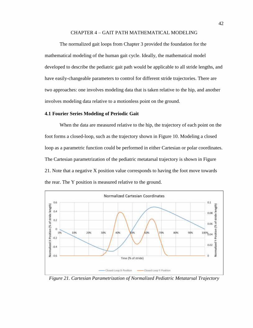
42
CHAPTER 4 – GAIT PATH MATHEMATICAL MODELING
The normalized gait loops from Chapter 3 provided the foundation for the
mathematical modeling of the human gait cycle. Ideally, the mathematical model
developed to describe the pediatric gait path would be applicable to all stride lengths, and
have easily-changeable parameters to control for different stride trajectories. There are
two approaches: one involves modeling data that is taken relative to the hip, and another
involves modeling data relative to a motionless point on the ground.
4.1 Fourier Series Modeling of Periodic Gait
When the data are measured relative to the hip, the trajectory of each point on the
foot forms a closed-loop, such as the trajectory shown in Figure 10. Modeling a closed
loop as a parametric function could be performed in either Cartesian or polar coordinates.
The Cartesian parametrization of the pediatric metatarsal trajectory is shown in Figure
21. Note that a negative X position value corresponds to having the foot move towards
the rear. The Y position is measured relative to the ground.
Figure 21. Cartesian Parametrization of Normalized Pediatric Metatarsal Trajectory

43
The Cartesian parametrization shows a periodic function for the X location that
appears to be generally sinusoidal. This is easily modeled as a sum of sinusoids using a
Fourier series. If 𝑓(𝑡) is the function giving the X coordinate, the Fourier series is given
in Equation 4-1.
𝑓(𝑡) = ∑ 𝑎𝑚 cos (2𝜋𝑚𝑡
𝑇) + ∑ 𝑏𝑛 sin (
2𝜋𝑛𝑡
𝑇)
∞
𝑛=1
∞
𝑚=0
Equation 4-1. Fourier Series Equation
where T is the period, and 𝑎𝑚 and 𝑏𝑛 are constants determined by the shape of the
function. Since this is normalized, we use normalized time units 𝜏 = 𝑡/𝑇. This changes
Equation 4-1 into Equation 4-2.
𝑓(𝑡) = ∑ 𝑎𝑚 cos(2𝜋𝑚𝜏) + ∑ 𝑏𝑛 sin(2𝜋𝑛𝜏)
∞
𝑛=1
∞
𝑚=0
Equation 4-2. Normalized Fourier Series Equation
The first term of the infinite series occurs when m=0 and is given by 𝑎0. The first
term is a constant, and constitutes the average of the equation. The expression for 𝑎0 is
given in Equation 4-3.
𝑎0 =1
𝑇∫𝑓(𝜏)𝑑𝜏
1
0
Equation 4-3. First Term in Fourier Infinite Series
To determine the values of all 𝑎𝑚 and 𝑏𝑛 to define this function, Equation 4-4 is
applied.

44
𝑎𝑚 =2
𝑇∫𝑓(𝜏) sin(2𝜋𝑚𝜏) 𝑑𝜏
1
0
𝑏𝑛 =2
𝑇∫𝑓(𝜏) sin(2𝜋𝑛𝜏) 𝑑𝜏
1
0
Equation 4-4. Concurrent Terms in Fourier Infinite Series
The terms are normalized through the period. The resulting equation will be
scalable by the period to attain the correct stride timing.
The results of Equation 4-4 can be placed into Equation 4-1 to create the full
model. The resulting equation for the mathematical model of any foot point trajectory is
given by Equation 4-5.
𝑋(𝑡) =𝐿
𝑇∑ 𝑎𝑚,𝑥 cos(2𝜋𝑚𝜏) + ∑ 𝑏𝑛,𝑥 sin(2𝜋𝑛𝜏)
∞
𝑛=1
∞
𝑚=0
𝑌(𝑡) =𝐿
𝑇∑ 𝑎𝑚,𝑦 cos(2𝜋𝑚𝜏) + ∑ 𝑏𝑛,𝑦 sin(2𝜋𝑛𝜏)
∞
𝑛=1
∞
𝑚=0
Equation 4-5. Cartesian Parametrization Using Fourier Series
where 𝜏 is the normalized time value equal to the percent of stride time, T is the stride
time, and L is the stride length. Note that while perfectly accurate results will be obtained
when m=∞ and n=∞, Fourier transforms tend to converge rapidly, and only a few orders
of calculation are needed to produce close approximations.
4.2 Metatarsal Trajectory Modeling
4.2.1 Cartesian Pediatric Gait Modeling
The pediatric gait data shown in Figure 21 were put into Equation 4-5, and the
constants were determined from Equation 4-4. To determine the goodness of fit, the R2
value (also known as the Coefficient of Determination) was calculated for each Fourier
order. To calculate the R2 value, the following equation is applied:

45
𝑅2 = 1 −∑ (𝑦𝑖 − 𝑓𝑖)
2𝑖
∑ (𝑦𝑖 − �̅�)2𝑖
Equation 4-6. R2 Calculation for Fourier Regression
where 𝑦𝑖 is the individual, measured data points, 𝑓𝑖 is the Fourier calculated data points
corresponding to the times of the measured data points, and �̅� is the average of all 𝑦𝑖
measured data points. Another way of viewing Equation 4-6 is the sum of squared error
measurements divided by the total sum of squares, which is correlated with the overall
data variance.
The Cartesian pediatric data series converged quickly, and each parametrized
value had an R2 value that approached 1 with increasing order of the Fourier series. It
was noted that the R2 value was over 99.0% for two orders of the Fourier X series and six
orders of the Fourier Y series (ox=2 and oy=6), and further orders of X and Y would only
improve the fit of the model. The resulting constants are shown in Table 5.
Table 5. Fourier Series Constants for Pediatric Cartesian Parametrization
Pediatric am and bn Constants
X-Coordinate R2
Y-Coordinate R2
m,n a b a b
0 0.00390 0.01885
1 -0.00149 0.44097 0.90534 -0.02920 -0.00245 0.61266
2 0.00345 -0.13606 0.99158 0.01023 0.00021 0.68802
3 -0.00359 0.04140 0.99963 0.00597 0.00571 0.73625
4 0.00255 -0.00695 0.99988 -0.01120 -0.00981 0.89382
5 -0.00104 -0.00201 0.99990 0.00750 0.00845 0.98476
6 0.00094 0.00363 0.99997 -0.00211 -0.00345 0.99644
7 -0.00053 -0.00120 0.99998 -0.00040 -0.00069 0.99690
8 0.00069 -0.00027 0.99998 0.00041 0.00173 0.99914
The resulting X and Y coordinates were plotted to determine visual closeness to
the original trajectories. The coordinates are plotted against normalized time and against
each other in Figures 22 and 23, respectively. The coordinates are plotted with Fourier

46
series orders ox=2 and oy=6. Note: further orders would improve the fit of the equations.
However, fewer Fourier series orders were used to show how well the curve was matched
at the R2 = 99.0% value. Full datasets from the pediatric, author, and Winter are shown in
Appendix A.
Figure 22. Mathematical Model of Normalized Cartesian Gait Coordinates (ox=2,oy=6)
Figure 23. Closed-Loop Trajectory of Cartesian Mathematical Model (ox=2,oy=6)
4.2.2 Polar Parametrization of Pediatric Data
The Cartesian coordinate modeling of the pediatric data proved successful, and
the convergence was good for lower orders of Fourier series. However, polar
parametrization of the gait path was conducted to compare to the Cartesian
parametrization.

47
For the polar parametrization, the location of the origin is very important. Placing
the origin changes the distance between the origin and the points on the curve, which can
create unique trajectories and profiles. Five points were identified as unique origin
locations. These five points are shown in Figure 24. Their coordinates, in units
normalized by the stride length, are shown as well.
Figure 24. Origin Locations for Analyzing Closed-Loop Polar Parametric Equations
The closed-loop trajectory was used to generate polar parametrizations at each
origin location. The resulting plots are shown in Figures 25 through 29.
Figure 25. Polar Parametrization of Metatarsal: Origin at Centerline Stride

48
Figure 26. Polar Parametrization of Metatarsal: Origin Leading Foot
Figure 27. Polar Parametrization of Metatarsal: Origin Trailing Foot

49
Figure 28. Polar Parametrization of Metatarsal: Origin at Hip
Figure 29. Polar Parametrization of Metatarsal: Origin Trailing Hip
Each of the trajectories shows a different profile curve. When the origin is located
at the centerline of the midstance stride (Figure 25), the angular position rapidly travels
toward 90 degrees as the profile loops back over the origin. This causes a small shift in
the otherwise smooth radial curve. The radial and angular displacements of the metatarsal
during stride are very similar when viewed from the leading and trailing foot positions.

50
The major difference is that the angular position is reversed, and there are small variances
in curve shapes.
The movement relative to the hip is more complicated. While the angular
displacement is smooth and shows gradual, gentle shift in angular position, the radial
position appears to have two distinct peaks with a trough in between. This dataset was not
adjusted for the vertical movement of the hip. According to Fang and Hunt, the toe
trajectory relative to the hip follows a near-circular path [92]. Fang and Hunt adjusted the
toe trajectories according to the vertical movement of the hip during gait. The resulting
circular trajectories of the toe are shown in Figure 30.
Figure 30. Circular Toe Trajectory Modeling [92]
Fang and Hunt continued the circular toe trajectory modeling with 24 subjects,
and showed that the circular model was a simple approximation based on hip height,
although the results were fairly diverse [93]. Further results for circular modeling of the
toe trajectory relative to the hip are shown in Figure 31. In each case, the dotted, circular-
shaped line was generated by the height of the hip.

51
Figure 31. Multi-Subject Circular Toe Trajectory Modeling [93]
While hip data were not provided for the datasets analyzed in this chapter, it is
believed based on Figure 30 that adjustment for hip movement would result in a flat path
for Figure 28 and only one trough without any ridges. This would make the hip an ideal
location for placing the origin and constructing a mathematical model of the heel,
metatarsal, and toe trajectories. However, without measuring hip movement, Figure 28 is
not smooth.
Figure 29 shows two periodic, smooth functions describing the radial and angular
displacement. Unlike the rest of the plots, Figure 29 has only two distinct peaks per line,
and both look very easy to model. As a result, Equation 4-5 can be rewritten to account
for radial and angular data. Note: The data was normalized using longitudinal stride
length, which is an easily-measured variable.

52
𝑅(𝑡) =𝐿
𝑇∑ 𝑎𝑚,𝑥 cos(2𝜋𝑚𝜏) + ∑ 𝑏𝑛,𝑥 sin(2𝜋𝑛𝜏)
∞
𝑛=1
∞
𝑚=0
𝜃(𝑡) =𝐿
𝑇∑ 𝑎𝑚,𝑦 cos(2𝜋𝑚𝜏) + ∑ 𝑏𝑛,𝑦 sin(2𝜋𝑛𝜏)
∞
𝑛=1
∞
𝑚=0
Equation 4-7. Radial Parametrization Using Fourier Series
The constants 𝑎𝑚 and 𝑏𝑛 were calculated for both R and θ values. The resulting
constants are shown in Table 6. Note that the R2 values decrease with increasing orders
after the third order of both X and Y. While the calculations were extensively checked,
the cause of this abnormality was not determined.
Table 6. Fourier Series Constants for Pediatric Polar Parametrization
Pediatric Polar am and bn Constants
X-Coordinate R2
Y-Coordinate R2
m,n a b a b
0 -2.13136 45.68394
1 -0.04022 0.30912 0.88457 0.66166 8.57807 0.89497
2 -0.00675 -0.09707 0.96962 -0.07062 -2.66329 0.98286
3 -0.03224 0.03515 0.97445 0.75052 0.68608 0.98487
4 -0.02880 -0.01261 0.96881 0.62797 0.06254 0.98070
5 -0.02260 0.00432 0.96195 0.46719 -0.20970 0.97711
6 -0.02769 0.00060 0.95449 0.60927 0.14438 0.97293
7 -0.02632 -0.00162 0.94692 0.54118 -0.01411 0.96846
8 -0.02589 0.00114 0.93920 0.57838 -0.03921 0.96385
Unlike the Cartesian parametrization and model, the polar parametrization did not
produce an acceptable curve. Using ox=3 and oy=3 (the closest fit according to R2
analysis with the Fourier analysis), the radial and angular mathematical positions were
calculated. The resulting curves are shown in Figure 32.

53
Figure 32. Mathematical Approximation of Polar Parametrization (ox=2,oy=6)
The mathematical model of the polar parametrization did not come out properly,
despite following the Fourier transform process. While higher-order Fourier series terms
usually cause an increase in trajectory accuracy, the R2 accuracy value dropped with
increasing order of Fourier series. One explanation as to why the Fourier series had
difficulty modeling this curve is that the actual curve approximates near-straight lines.
Fourier series struggle to model straight lines, and require higher order numbers, possibly
significantly higher frequency terms. While further work may more closely approximate
this curve, it was determined that closed-loop modeling was best conducted using
Cartesian coordinates.
4.2.3 Fourier Series Modeling of Author’s Data
Equation 4-5 was applied to the Author’s data shown in Figure 10. The constants
determined from Equation 4-4 are shown in Table 7. Similar to what was seen in the
pediatric dataset, the series appeared to converge nicely, and had above a 99.0% R2 value
with ox=2 and oy=6. Full Cartesian parametric data is shown in Appendix A.

54
Table 7. Fourier Series Constants for Cartesian Modeling of Author's Data
Author's am and bn Constants
X-Coordinate R2
Y-Coordinate R2
m,n a b a b
0 0.00128 0.03628
1 -0.00084 0.43503 0.93211 -0.04992 0.00587 0.63050
2 0.00102 -0.11515 0.99742 0.00469 -0.01255 0.67530
3 -0.00414 0.01565 0.99871 0.02245 0.01583 0.86325
4 0.00684 0.00999 0.99943 -0.01789 -0.01199 0.97894
5 -0.00545 -0.00753 0.99986 0.00113 0.00427 0.98382
6 0.00132 0.00134 0.99988 0.00661 0.00076 0.99485
7 0.00190 0.00246 0.99992 -0.00372 -0.00128 0.99872
8 -0.00240 -0.00226 0.99998 -0.00055 0.00037 0.99883
4.2.4 Fourier Series Modeling of Winter’s Data
Equation 4-5 was applied to Winter’s data shown in Figure 13 [91]. The constants
determined from Equation 4-4 are shown in Table 8. Similar to what was seen in the
pediatric dataset, the series converged nicely with an R2 value of 99.0% or higher at ox=2
and oy=6. Full Cartesian parametric data are shown in Appendix A.
Table 8. Fourier Series Constants for Cartesian Parametrization of Winter’s Data
Winter's am and bn Constants
X-Coordinate R2
Y-Coordinate R2
m,n a b a b
0 0.00055 0.03505
1 -0.00711 0.44439 0.95824 -0.04216 0.00115 0.58105
2 0.00426 -0.09081 0.99836 -0.00722 -0.01001 0.62845
3 -0.00304 0.00772 0.99870 0.02340 0.01643 0.89298
4 0.00425 0.01054 0.99932 -0.01039 -0.01303 0.98326
5 0.00080 -0.00195 0.99935 -0.00266 0.00141 0.98595
6 -0.00015 0.00074 0.99936 0.00366 0.00317 0.99409
7 0.00044 0.00292 0.99940 0.00057 -0.00081 0.99442
8 -0.00233 0.00074 0.99940 -0.00171 -0.00003 0.99524
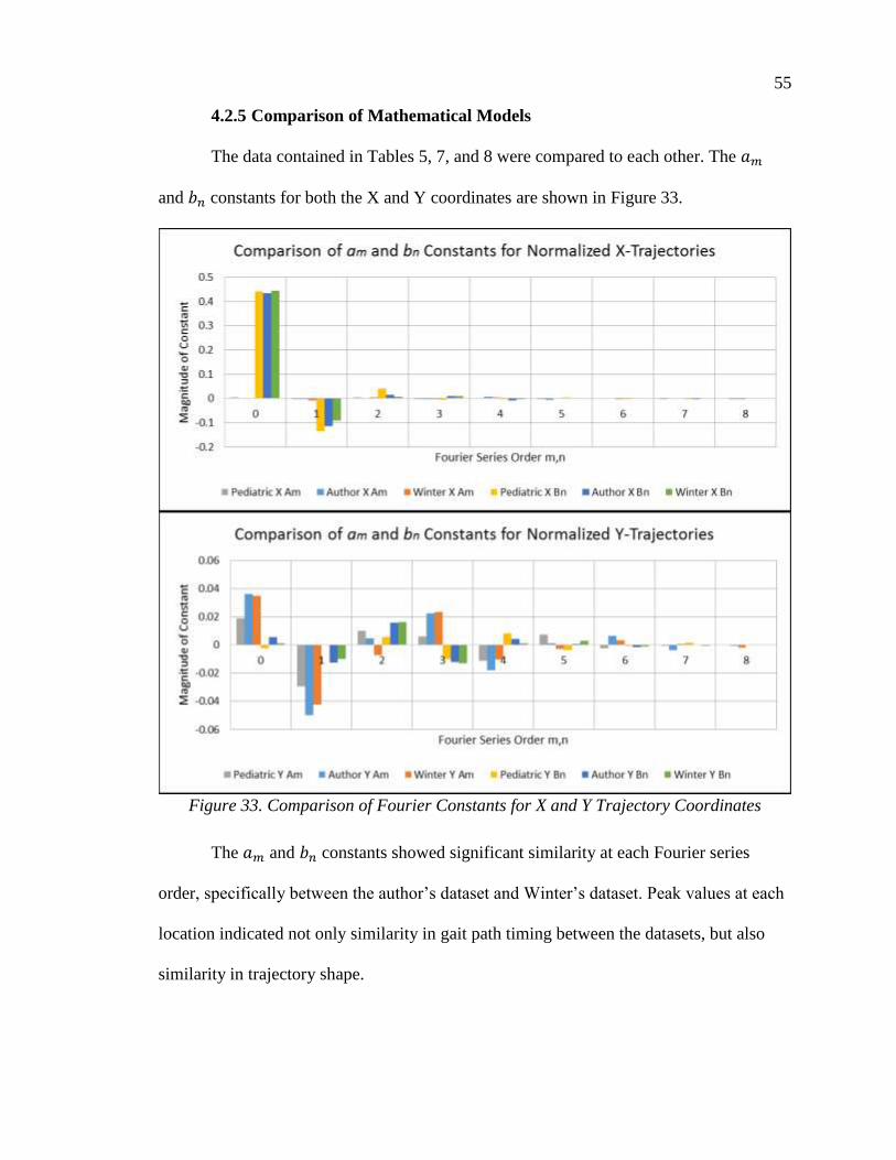
55
4.2.5 Comparison of Mathematical Models
The data contained in Tables 5, 7, and 8 were compared to each other. The 𝑎𝑚
and 𝑏𝑛 constants for both the X and Y coordinates are shown in Figure 33.
Figure 33. Comparison of Fourier Constants for X and Y Trajectory Coordinates
The 𝑎𝑚 and 𝑏𝑛 constants showed significant similarity at each Fourier series
order, specifically between the author’s dataset and Winter’s dataset. Peak values at each
location indicated not only similarity in gait path timing between the datasets, but also
similarity in trajectory shape.

56
An average was taken of the pediatric, author’s and Winter’s dataset Fourier
series constants. Using these new constants and Equation 4-5, a new trajectory was
developed. The Fourier series constants are shown in Table 9. The resulting parametric
coordinates are shown in Figure 34, and the resulting traced trajectory is given by Figure
35. Unlike previous Fourier series constants, the error in these was unmeasurable. Thus,
order values of ox=8 and oy=8 were used to improve smoothness. Full Cartesian
parametric data is shown in Appendix A.
Table 9. Fourier Series Average Metatarsal am and bn Constants
Average Metatarsal Am and Bn Constants
X-Coordinate Y-Coordinate
m,n a b a b
0 0.001952 0.030684
1 -0.00321 0.449314 -0.04127 0.001555
2 0.002967 -0.11639 0.00262 -0.0076
3 -0.00367 0.022039 0.017633 0.01292
4 0.004643 0.004623 -0.01344 -0.01185
5 -0.00193 -0.00391 0.002033 0.004808
6 0.000715 0.001944 0.002778 0.000164
7 0.000618 0.001426 -0.00121 -0.00095
8 -0.00138 -0.00061 -0.00063 0.000702

57
Figure 34. Fourier Series Average Metatarsal Trajectory Parametrization (ox=8,oy=8)
Figure 35. Fourier Series Average Metatarsal Trajectory (ox=8,oy=8)
The average curve showed very high similarities with all three curves, and the
timing curves showed similarities with all three curves as well. Ideally, more Fourier
series terms would be included in the average. However, given the data present, it was
decided that this averaged model of the three datasets would be used as the “ideal”
metatarsal trajectory path to model for the gait machine.
4.3 Heel Profile
A Fourier analysis was conducted on the heel trajectory of each of the three
datasets. Similar to the metatarsal analysis, the heel profiles were calculated to 8 orders of

58
the Fourier series. For each of these three data sets, it was discovered that the Fourier
series converged very quickly, reaching R2 values of 99.0% or greater within three
orders. As such, plots were made of each of the profiles using ox=2 and oy=3 to show
convergence. The results of the pediatric, author’s dataset, and Winter’s dataset Fourier
analysis of the heel data are shown in Figures 36 through 38. Note that despite the high
convergence, the mathematical model and full heel trajectories were fairly different. Part
of this is due to the low order count that was plotted. Part of this is due to the larger data
variance. Full Cartesian knee modeling is shown in Appendix A.
Figure 36. Parametric Modeling of Pediatric Heel Data (ox=2,oy=3)

59
Figure 37. Parametric Modeling of Author’s Heel Data (ox=2,oy=3)
Figure 38. Parametric Modeling of Winter's Heel Data (ox=2,oy=3)
Often, the mathematical approximation of the curve proved to be much smoother
than the actual dataset. This occurs when real measurements are inaccurate, are recorded
with limited accuracy, and require heavy filtering to obtain realistic results. In these
cases, highly-accurate curve modeling is undesirable, and a smooth, general curve is
preferred.

60
The 𝑎𝑚 and 𝑏𝑛 constants were averaged between the author’s, Winter’s, and
pediatric datasets. The resulting 8-order averages are shown in Table 10. The
mathematically averaged heel trajectories were plotted parametrically and against each
other in Figures 39 and 40.
Table 10. Fourier Series Average Heel am and bn Terms
Average Heel am and bn Constants
X-Coordinate Y-Coordinate
m,n a b a b
0 0.040722 0.084108
1 -0.0771 0.447013 -0.12761 0.064313
2 0.050769 -0.07244 0.055108 -0.06419
3 -0.02075 -0.01306 -0.01068 0.033135
4 0.003907 0.017561 -0.00143 -0.00955
5 0.002082 -0.00021 0.000826 -0.00077
6 -0.00074 -0.00299 0.000967 0.002664
7 0.000463 0.00262 -0.00094 -0.00054
8 -0.00056 0.00139 0.000245 -0.00074
Figure 39. Fourier Series Average Heel Trajectory Parametrization (ox=8,oy=8)

61
Figure 40. Fourier Series Average Heel Trajectory (ox=8,oy=8)
4.4 Foot Angle Modeling
Using the raw metatarsal and heel data from the author’s, Winter’s, and the
pediatric data sets, the foot angle was calculated. The foot angles were zeroed such that
the foot was flat during most of stance. The convergence varied between datasets. The
pediatric set reached an R2 value of 99.0% in 3 orders, Winter’s dataset convergence in 4
orders, and the author’s dataset reached convergence in 5 orders. The mathematical
models were compared to the actual data for each of these three datasets in Figures 41
through 43. The full analysis of the foot angle is shown in Appendix A.

62
Figure 41. Pediatric Foot Angle Data Mathematical Modeling (ox=3)
Figure 42. Author's Foot Angle Data Mathematical Modeling (ox=5)

63
Figure 43. Winter's Foot Angle Data Mathematical Modeling (ox=4)
The foot angle Fourier series were averaged between the three datasets. The
resulting 𝑎𝑚 and 𝑏𝑛 averages are shown in Table 11. The foot angle traced by the average
mathematical approximation is compared to the actual datasets in Figure 44.
Table 11. Average Fourier Series Constants for Foot Angle Modeling
Average Foot Angle am and bn Constants
X-Coordinate
m,n a b
0 11.80293
1 -14.8457 23.02922
2 2.166785 -19.1956
3 1.193393 4.867124
4 -0.49204 2.551773
5 -0.0414 -2.13996
6 0.216997 -0.06041
7 -0.07251 0.79371
8 -0.11119 -0.46419
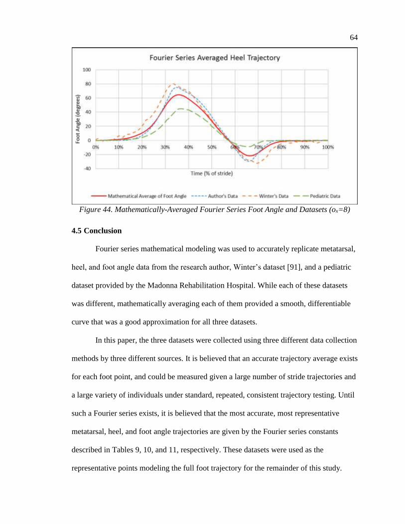
64
Figure 44. Mathematically-Averaged Fourier Series Foot Angle and Datasets (ox=8)
4.5 Conclusion
Fourier series mathematical modeling was used to accurately replicate metatarsal,
heel, and foot angle data from the research author, Winter’s dataset [91], and a pediatric
dataset provided by the Madonna Rehabilitation Hospital. While each of these datasets
was different, mathematically averaging each of them provided a smooth, differentiable
curve that was a good approximation for all three datasets.
In this paper, the three datasets were collected using three different data collection
methods by three different sources. It is believed that an accurate trajectory average exists
for each foot point, and could be measured given a large number of stride trajectories and
a large variety of individuals under standard, repeated, consistent trajectory testing. Until
such a Fourier series exists, it is believed that the most accurate, most representative
metatarsal, heel, and foot angle trajectories are given by the Fourier series constants
described in Tables 9, 10, and 11, respectively. These datasets were used as the
representative points modeling the full foot trajectory for the remainder of this study.

65
CHAPTER 5 – PEDIATRIC INTELLIGENTLY-CONTROLLED ASSISTIVE
REHABILITATION ELLIPTICAL
Pediatric models of rehabilitation machines exist (such as treadmills and pediatric
ellipticals). However, pediatric rehabilitation machines are not as common as adult
machines because of the limited use. Since adult machines can service individuals from
around age 12 onward, adult machines have a significantly larger target population. This
means that having a designated pediatric machine takes up more space and cost in the
facility. Illness, injury, surgery, and other causes of pediatric immobility and gait issues
can have long-lasting effects on the individual if not treated as a child, giving a great
weight to pediatric rehabilitation.
In order to make a pediatric rehabilitation machine cost-effective, the machine
would have to serve both children and adults in their rehabilitation needs. This limits the
amount of equipment needed to be purchased and the overall space required for dealing
with both patient age groups. As per requests from experts at Madonna Rehabilitation
Hospital, the device would have to accommodate stride lengths from 8 inches to 30
inches at least.
5.1 Pediatric Considerations
Modifying an existing system to account for pediatric use requires several
considerations. Any pediatric device accommodating the large range of sizes and weights
of the varying age group must take into account the normalization factors. According to
Hof, each of the gait parameters can be defined in terms of body mass, leg length,
cadence, and the gravitational constant [17]. For a retrofitted, existing adult gait therapy
mechanism, the mechanism usually has a method of accounting for differing body
66
weights and cadence. Thus, the major pediatric concern is leg length. Sutherland noted
that the leg length and stride length showed strong correlation [18].Thus, the
normalization factors can be reduced to only considering stride length, as long as the
machine already accounts for varying weights and cadences. Many gait machines already
allow a broad range of cadences and are constructed to handle a broad range of patient
weights.
There are more physical (anthropometric) considerations that should be made in
modifications to an adult gait therapy machine to accommodate pediatric patients.
Children differ from adults in the lateral distance between feet when walking. Having
foot pedals too far apart would discourage normal gait activity in children. Also, the
maximum foot height during the swing phase of gait is significantly smaller for pediatric
patients than adults. Any handles or a console that is used for user stability and/or
interaction is going to be at differing heights for adults and small children. Adjustments
for all three of these distances would be beneficial.
5.2 ICARE System
The Intelligently-Controlled Assistive Rehabilitation Elliptical (ICARE) has
proven to effectively rehabilitate adults with little effort from the physical therapist
[70,80-83,94-97]. The success of the robotic elliptical machine shows that using a system
that constrains the foot motion may be as effective as complicated, expensive systems or
therapist-intensive rehabilitation methods. Since walking is the primary form of exercise
for the bipedal human, the ICARE provides an opportunity for people with little-to-no
walking ability to still engage in physical exercise, making it ideal for children who may
require significant assistance in walking.

67
The full ICARE system involves an elliptical device, a set of ramps and a seat to
assist in mounting the device and reaching the pedals, and an overhead body-weight
suspension system. The elliptical device and the full system are shown in Figure 45.
Figure 45. ICARE by SportsArt

68
5.2.1 ICARE Kinematics and Redesign
The ICARE elliptical device consists of a foot pedal riding along a curved bar
attached to a crank-rocker four-bar linkage. The foot pedal is mounted to the rocker,
whereas the curved, round bar is mounted to the crank. The mounting positions and a
dissected view of the coupler and curved bars are shown in Figure 46.
Figure 46. ICARE Coupler and Curved Bars
For the consideration factors listed in Section 5.1, the ICARE stride length is
dependent on the height of the connection of the coupler bar to the rocker and the length
of the crank. Currently, to adjust for various adult gait lengths, the height of the coupler
along the rocker is adjusted while the crank remains fixed. This provides adjustment
between 29 in. and 18.5 in. for the stride length in the commercially available version of
the ICARE. However, it does not accommodate for stride lengths as small as 8 in., which
is the target range of pediatric stride lengths. Thus, to adjust the stride length of the
ICARE, modifications will need to be made to the crank.
The foot height during use is highly dependent on the movement of the crank and
the profile of the curved bar that the foot pedal rides on. As was previously stated, the
crank will be adjusted to modify the stride length. Following adjustments to the crank, the
foot path height will be assessed to determine whether further changes are needed to the
curved bar.

69
The lateral distance between foot pedals is a concern. While the foot pedals could
be redesigned to slide inward, it was decided that new mounts would allow for the foot
pedals to be moved inward. These were designed and installed by Madonna
Rehabilitation Hospital staff after the completion of the crank redesign.
5.3 Crank Design
The existing crank is a solid metal piece that is rigidly attached to the axle using a
set pin and connects to the end of the coupler bar with a revolute joint. To adjust the
length of the crank, the distance between the axle and the revolute joint must be variable.
A three-piece mechanism was designed to replace the crank. The new crank
mechanism consists of a mobile axle connection bracket, a screw and collar, and a slotted
crank. The screw is connected to the crank through a revolute joint and constrained with
the collar. The other end of the screw is threaded into a tapped hole on the axle
connection bracket. The axle connection bracket slides along the crank freely, forming a
prismatic joint. As the screw turns, it freely rotates in the revolute joint and moves the
axle connection bracket vertically relative to the crank. With this design, axial load is
transferred from the crank to the axle connection bracket through the screw, while shear
and bending loading is transmitted directly from the crank to the connection bracket. The
new and old crank designs are compared in Figure 47.

70
Figure 47. Existing and Proposed ICARE Crank Designs
When designing modifications to an existing system, it is important that the
impact of the new pieces be assessed on the existing machine. Ideally, the modified crank
would integrate into the system without contacting or disrupting the function of any other
component. Due to the presence of the motor overhead and electrical components in the
rear of the machine, the crank length could not be extended from the original length. The

71
screw was located on the side of the axle connection bracket and the crank for this
reason.
On the original design, the distance between the center of the axle and the crank
revolute joint with the coupler bar was 8.25 in. On the new design, the center-to-center
distance could be adjusted from 8.25 in. to 3.25 in.
As the stride length decreased, the height of the foot path also decreased
significantly. Foot pedal paths of the modified mechanism are shown in Figure 48. The
trajectory of the foot pedal was very similar between the shortest crank length and the
largest crank length. After normalizing the trajectories based on the stride length, there
were only minor variances in trajectory, as shown in Figure 49. Since normalized child
gait data strongly resembled adult gait, similar normalized elliptical paths should be
beneficial to pediatric patients. Hence, the new crank mechanism design was determined
to successfully reproduce the gait training used in adults for pediatric patients. It should
be noted that physical testing is necessary to conclude that this therapy carries the same
benefits for children as for adults.
Figure 48. Foot Pedal Paths for Varying Crank Lengths

72
Figure 49. Normalized Foot Pedal Trajectories for Varying Crank Lengths
5.4 Screw Selection
The modified ICARE was designed to have a maximum weight limit of 250 lb.
When the body weight support feature is not used, the patient pivots from one foot to the
other, applying the full body weight to both pedals in each gait cycle. The proximity of
the foot pedals to the rocker mechanism means that much of the patient’s weight will be
carried by the rocker, limiting the loading on the crank. For safety purposes, the crank
mechanism was designed assuming that the entire weight of the patient was placed on the
coupler right next to the revolute joint connection with the crank.
5.4.1 Screw Calculations
According to the design, the maximum load imparted on the screw occurs when
the screw is in the vertical position. In these positions, the screw resists unscrewing and
the threads must not fail. During one cycle, the screw carries all of the weight of the
patient and coupler bar in tension and compression. The axial stress in the screw is given
by
𝜎𝑎 =𝐹
𝐴𝑒𝑓𝑓
=4𝐹
𝜋𝑑𝑟2
Equation 5-1. Screw Axial Stress

73
where 𝜎𝑎 is the axial stress, F is the axial force, 𝐴𝑒𝑓𝑓 is the effective cross-sectional area
of the solid central shaft of the screw, and 𝑑𝑟 is the diameter of the solid central shaft of
the screw. Here, 𝐴𝑒𝑓𝑓 is used because axial stress is not carried across the open threads.
The most critical loading location on the screw is the thread contact between the
screw and the mobile bracket. According to Budynas and Nisbett, experiments with
screws have shown that only the first seven engaged threads carry weight, and the first
engaged thread carries 38% of the load, with subsequent threads carrying less [98]. Using
this loading scenario, the screw hand calculations were performed. A diagram of the
simple loading and constraints on the screw is shown in Figure 50.
Figure 50. Simple Screw Loading for Screw Selection Calculations
Since the screw contact occurs on the threads, the force occurs on an off-axis
incline and lateral and shear forces exist. The force labels on the screw are labeled in
Figure 51. The lateral and shear forces are given by
𝜎𝑥 =6𝐹
𝜋𝑑𝑟𝑛𝑡𝑝
𝜏𝑦𝑧 =16𝑇
𝜋𝑑𝑟3
Equation 5-2. Screw Lateral and Shear Forces [98]
where 𝜎𝑥 is the lateral force, 𝜏𝑦𝑧 is the shear force, 𝑛𝑡 is the number of threads engaged, p
is the pitch, and T is the torque required to turn the screw against the applied force. To

74
determine maximum stresses at the joint between the screw and the axle connection
bracket, substitute 0.38F for the force and let 𝑛𝑡 be 1 thread [98].
Figure 51. Screw Stress Orientations
The torque T is given by
𝑇 =𝐹𝑑𝑚
2(𝑙 + 𝜋𝑓𝑑𝑚 sec 𝛼
𝜋𝑑𝑚 − 𝑓𝑙 sec 𝛼) +
𝐹𝑓𝑐𝑑𝑐
2
Equation 5-3. Torque Required To Turn Screw Against Applied Load [98]
where 𝑑𝑚 is the pitch diameter, f is the coefficient of static friction between the bracket
and the screw, l is the screw lead, α is the thread angle, 𝑓𝑐 is the coefficient of friction
between the bracket and the collar, and 𝑑𝑐 is the mean collar diameter.
Designing and implementing a new screw is difficult and costly. Thus, these
calculations were performed on existing commercially available screws. To determine the
constants for the calculations, different diameters and pitches of ACME screws were
compared to each other.
A fatigue analysis was conducted so that the screw would survive an infinite
number of cycles. Different fatigue models exist, but one of the more stringent models
was developed by Soderburg [99]. According to the Soderburg model of fatigue,
𝑆𝐹 =𝜎∞
𝜎𝑎[1 − (
𝜎𝑚
𝜎𝑦)]
Equation 5-4. Fatigue Safety Factor Determination

75
where
SF is the safety factor
𝜎𝑎 is the amplitude of stress variation away from 𝜎𝑚
𝜎∞ is the maximum material strength at infinite stress cycles
𝜎𝑚 is the mean cyclic stress applied to the material
𝜎𝑦 is the yield stress of the material
5.4.2 Selected Screw Description
A 3/8-12 ACME threaded screw was selected. The calculation parameters for the
screw are shown in Table 12.
Table 12. 3/8-12 ACME Threaded Screw Parameters
Variable Description Value
dn Nominal screw diameter 0.3750 in.
dr Minor diameter of screw 0.2917 in.
dm Pitch diameter 0.3333 in.
p Pitch 0.08333 in.
l Lead 0.2708 in.
α Thread angle 14.5 deg
f Static friction coefficient
between screw and bracket 0.08
fc Friction coefficient between
collar and bracket 0.08
dc Mean collar diameter 0.5 in.
Using F = 270 lb, the maximum torque, axial, lateral, and shear forces are
𝑇 = 21.09 𝑙𝑏 − 𝑖𝑛
𝜎𝑎 = 4,040.18 𝑝𝑠𝑖 𝜎𝑥 = 8,061.12 𝑝𝑠𝑖

76
𝜏𝑦𝑧 = 4,327.53 𝑝𝑠𝑖
The Von Mises stress is given by
𝜎𝑣𝑚 = [(𝜎1 − 𝜎2)
2 + (𝜎2 − 𝜎3)2 + (𝜎3 − 𝜎1)
2
2]
Equation 5-5. Von Mises Stress Calculation [98]
where 𝜎1, 𝜎2, and 𝜎3 are the principle stresses of the system, which can be determined by
reducing the stress matrix into row echelon form. Using this formula, the Von Mises
stress was 14,485 psi, and the maximum shear stress is 5,408 psi. Assuming that the
threaded rod material is tempered steel with a minimum tensile strength of 97,300 psi,
using the Von Mises method, the factor of safety for a 270-lb axial load on a 3/8–12
ACME threaded rod would be 6.7173. For fatigue loading, 𝜎𝑚=0 psi and 𝜎𝑎 is the Von
Mises maximum stress of 14,485 psi. According to Budynas and Nesbit, the infinite
stress 𝜎∞ for tempered steel is 49,300 psi. Using Equation 5-4, the axial loading and
unloading of the threaded rod would result in a fatigue safety factor of 3.4035.
Some bending would occur in the threaded rod based on the loading
configuration. The effects of the bending load are important to consider, and should be
evaluated for their effect on the system.
5.5 Simulation Model and Method
The crank, axle connection bracket, and screw were modeled using the LS-DYNA
explicit, nonlinear, finite-element simulation software from Livermore Software
Technology Corporation [100].
Each component was modeled as A36 steel under elastic loading. Components
were constructed of 5 mm long cubic solid elements. Load was applied uniformly at the
revolute joint between the crank and the coupler. The axle was simulated as a rigid

77
cylinder passing through the crank mechanism. The axle connection bracket was rigidly
attached to the axle, while the crank was allowed to rotate about the axle. The 3/8–12
screw was simplified as a 0.2917-in. diameter tube rigidly attached to the crank and the
axle connection bracket. The component names and loading locations for the simulation
are shown in Figure 52. The simulation model is shown in Figure 53. Note that the circle
on the left represents the rigid axle connection to the mobile bracket and the circle on the
right represents the simulated coupler connection, which was used as a site to apply an
average pressure summing to 270 lb on the lever arm.
Figure 52. Component Labels and Loading Locations
Figure 53. Simulated Crank, Bracket, and Screw

78
Initial simulations showed that the position of the axle (represented by the rigid
blue circle in Figures 52 and 53) affected the stresses on the crank and the maximum
stress seen in the system. After several adjustments, it was noticed that the maximum
stress in the system was observed when the axle was located 0.25 in. away from the inner
edge of the slot. Also, it was observed that beginning the simulation with the axle only in
contact with the bracket (not the crank itself) would increase the maximum stress as well.
This case could be seen in manufacturing if the tolerances for the axle and the slot are
insufficient. This configuration was used for all testing.
In physical testing, surface finish, material type, presence of particulates, and
many other factors contribute to the friction between two surfaces. Friction due to
penalty-based contact in finite element simulations can be difficult to calculate. To gather
a full picture of the effects of friction on a system, the coefficient of friction between the
components must be analyzed. Based on the results of the friction study, the friction
coefficient is chosen to maximize the stresses in the system. This method tends to
produce conservative estimates of contact forces. During the course of the simulations, it
was discovered that the friction between the axle connection bracket and the crank
showed a significant effect on the maximum stress. The friction coefficient was
decreased and the results were observed.
In penalty-based contact, contact forces are dependent on the mesh of the
component. Coarser meshes tend to produce higher contact forces and stresses, while
finer meshes tend to be “softer” and mitigate some of the hard points. The original, 5-mm
long mesh was refined to 1.6-mm long cubic solid elements for comparison.

79
A static analysis of the crank assembly was conducted. Weight was applied to the
crank mechanism in four directions corresponding to axial and transverse loading. The
maximum stresses in the crank and screw were noted for each simulation.
The crank assembly was also modeled dynamically. A rotational speed was
imparted on the crank mechanism, simulating the axle spinning. The crank rotated at a
rate of 1 rev/s while experiencing a constant downward load of 270 lb.
5.6 Simulation Results
During the static simulations, the maximum stresses were located around the
bottom of the slot of the crank, occurring along shear planes that extended from the
contact with the axle connection bracket. For the screw, the maximum stresses occurred
at the connection between the screw and the axle connection bracket.
It was found that reducing the friction between the crank and the axle connection
bracket increased the contact stresses in the crank, but decreased overall maximum
stresses in the system. Very low friction values are not expected in the real assembly,
however, and utilizing a higher-than-expected friction coefficient in the simulation yields
maximum stress values that are conservative.
For each simulation, removing the contact between the crank and the axle caused
higher stresses in the crank. Since the maximum stresses were observed around the slot in
each simulation, the axle contact was serving to strengthen the slot. Thus, the simulations
predict that if the tolerance between the crank and the axle is loose, the crank will
experience larger stress values.
The maximum observed Von Mises stress values for the statically-loaded, coarse-
mesh simulation models are shown in Table 13. In the vertical direction, loading the
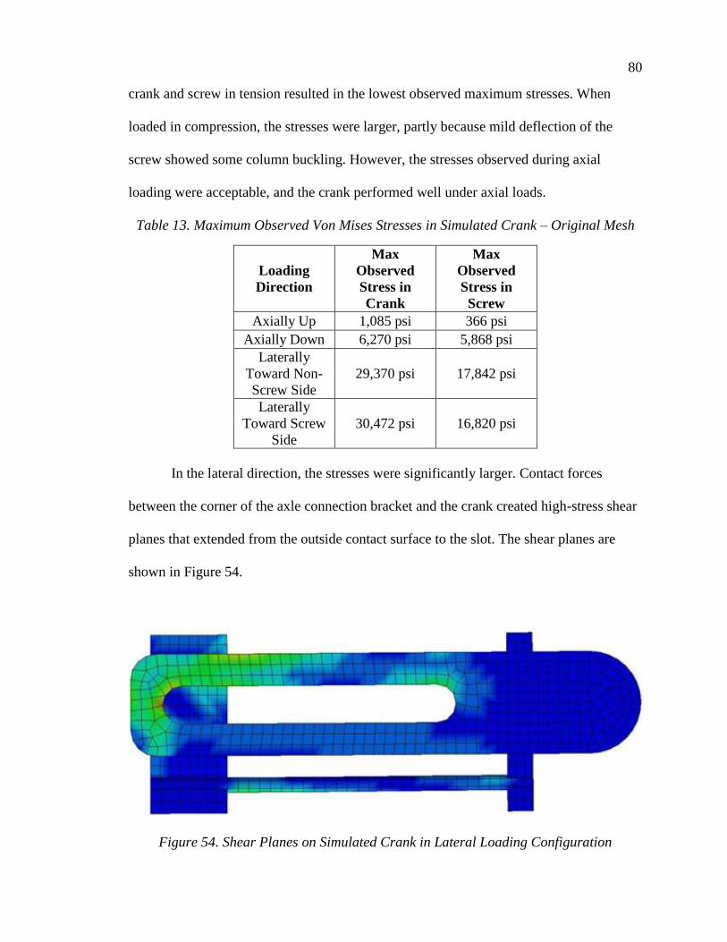
80
crank and screw in tension resulted in the lowest observed maximum stresses. When
loaded in compression, the stresses were larger, partly because mild deflection of the
screw showed some column buckling. However, the stresses observed during axial
loading were acceptable, and the crank performed well under axial loads.
Table 13. Maximum Observed Von Mises Stresses in Simulated Crank – Original Mesh
Loading
Direction
Max
Observed
Stress in
Crank
Max
Observed
Stress in
Screw
Axially Up 1,085 psi 366 psi
Axially Down 6,270 psi 5,868 psi
Laterally
Toward Non-
Screw Side
29,370 psi 17,842 psi
Laterally
Toward Screw
Side
30,472 psi 16,820 psi
In the lateral direction, the stresses were significantly larger. Contact forces
between the corner of the axle connection bracket and the crank created high-stress shear
planes that extended from the outside contact surface to the slot. The shear planes are
shown in Figure 54.
Figure 54. Shear Planes on Simulated Crank in Lateral Loading Configuration

81
The mesh was refined, and a smaller mesh was used to simulate the lateral
loading of the crank mechanism. The finer mesh was approximately one third the length
of the coarse mesh. The crank mechanism showed similar stress distribution through the
crank between the coarse mesh and fine mesh models, but the fine mesh model
experienced significantly reduced stresses. Stress values are noted in Table 14.
Table 14. Maximum Observed Von Mises Stresses in Simulated Crank – Reduced Mesh
Loading
Direction
Max
Observed
Stress in
Crank
Max
Observed
Stress in
Screw
Laterally
Toward Non-
Screw Side
18,948 psi 12,590 psi
Laterally
Toward Screw
Side
17,827 psi 13,992 psi
The crank mechanism was rotated at 1 rev/s with a constant downward load
applied. The axle contact was included in this simulation, but it was determined that the
axle contact was the least critical case, and in further simulations, this contact was
ignored.
The loading on the lever arms caused vibration, and the stress did not vary
smoothly with time. Lower overall loads were observed during this simulation. The
maximum stress in the rotating bracketed lever arm was 16,244 psi and occurred in the
side of the crank above the axle connection bracket opposite the screw. The lever arm
was nearly vertical, and the slight angle caused bending moments to concentrate in the
side of the crank. However, this stress is lower than the stresses observed in static loading
of the bracketed lever arm design. Contact stresses were observed to be significantly
lower also. The maximum stress state of the rotating lever arm is shown in Figure 55.

82
Figure 55. Maximum Stress State During Dynamic Testing
5.7 Discussion
Simulation analysis showed that the new crank mechanism could experience peak
stress values of up to 30,500 psi in the crank and 17,800 psi in the screw. Low-grade, hot-
rolled steel has a yield strength of at least 33,000 psi. Thus, the crank mechanism would
not be able to be constructed from inexpensive steel.
It was decided that the crank mechanism should be constructed from cold-rolled
steel with a minimum yield strength of 60,000 psi. While this increases the cost
significantly, the safety factor of at least 1.97, combined with the conservative stress
estimates and loading conditions, means that the mechanism is unlikely to fail.
The simulation measured high bending stresses in the screw near the connection
to the axle connection bracket. As calculated earlier, the screw experiences significant
stresses under axial loading. Using Equation 5-4, the fatigue safety factor for the threaded
rod was determined to be 2.77. It should be noted that the simulation treated the
connection between the screw and the axle connection bracket as a fixed cantilever beam.
There was no ability to rotate, bend, or compress at the connection site. While this

83
doesn’t perfectly model the connection, it provides a conservative estimate of the stresses
experienced by the screw at that location as long as the other simulation constraints hold
to be true.
Simulation results showed that the design would not experience stresses above 35
kpsi. To be able to handle this load, it is recommended that the crank be constructed from
cold-rolled steel or other higher-strength steels.
5.8 Design Issues
The pediatric ICARE machine has been tested using children at Madonna
Rehabilitation Hospital. Several conference abstracts are available at the time of this
writing [101-103]. Following discussion with the researchers at Madonna Rehabilitation
Hospital, the pediatric ICARE appears to be functioning properly. After the results of this
testing period have been analyzed, the design will be re-assessed, and potential design
improvements will be suggested.
One problem was noted with the completion of this study. As stated earlier,
simulation results showed that the stress concentration in the crank increased when the
axle was not in contact with the slot of the crank. This led the crank to be designed with
minimal tolerance for the axle shaft in the slot. However, it was found that dust, debris,
and other foreign objects can cause the adjustment process to seize when amalgamated
around the axle in the crank slot. This caused the collar to slide down the length of the
screw when adjustments were made, creating contact problems and disabling the
machine. Using an ACME threaded nut welded to the shaft as a replacement for the collar
would prevent this slippage. This was found to be strong enough to overcome the dust in
the slot.

84
The tolerances on the moving bracket allowed the bracket to twist while sliding
along the crank, causing an irritating clanking noise during one stride cycle. Also, it was
discovered that the threads on the ACME threaded rod were grinding and producing
particulates, and this was making it difficult to turn and causing issues with adjustment.
To solve these issues, the tolerance on the inside of the bracket was decreased, and the
threaded rod diameter was increased from 0.375 in. to 0.5 in. The final design, installed
on the ICARE system, is shown in Figure 56. Drawings of the final pediatric ICARE
crank parts are shown in Appendix B.
Figure 56. Pediatric ICARE Final Design
5.9 Conclusions
The adult ICARE elliptical system was evaluated and modified to accommodate
pediatric patients as well as adult patients. The machine was developed by designing an

85
adjustable crank that allows for stride reduction from the claimed maximum of 30 in.
down to 7.5 in. Adjustment produces a nearly linear scaling of the adult elliptical stride
path for the foot.
The pediatric ICARE machine has been tested using children at Madonna
Rehabilitation Hospital. Several conference abstracts are available at the time of this
writing [101-103]. Following discussion with the researchers at Madonna Rehabilitation
Hospital, the pediatric ICARE appears to be functioning properly. After the results of this
testing period have been analyzed, the design will be re-assessed, and potential design
improvements will be suggested.

86
CHAPTER 6 – DETERMINATION OF GAIT REPLICATION METHOD
At the beginning of this project, researchers had two overarching design goals: (1)
to design a gait therapy machine that could accommodate pediatric and adult patients to
limit the number of therapy machines needed for a facility, and (2) to develop a machine
that more accurately mimics the trajectory of the foot during gait. Following the
successful development of the pediatric ICARE unit, it was noted that the gait profiles
from the new crank, shown in Figure 49, still show a very large gait height change per
stride, which is significantly different from the average gait profile shown in Figure 35.
Thus, a brand-new rehabilitation machine was developed.
6.1 Design Goals
A rehabilitation mechanism for use in a healthcare, rehabilitation, or home-health
setting would need to accommodate the setting so it doesn’t discomfort or endanger other
individuals around it. As such, a set of design goals were established. The primary design
goals for the project were:
• Gait-Like Trajectory: The mechanism must constrain the feet to a trajectory
similar to normal gait motion, as shown in Figures 35 and 40.
• Scalable: The mechanism must accommodate for individuals with a stride length
between 6 and 40 in. while producing an easily-scaled full foot trajectory
(including accurate foot angles) such that the size of the trajectory is scalable, but
the shape remains constant. Ideally, the scaling would be linear, as this is the
easiest form of scaling to understand. This would make sure that therapists using
the device can easily read and adjust the scale of the gait path to fit the user. Also,

87
the scaling process should be performed by one motive element, eliminating the
possibility of accidental misalignment or inaccurate mechanism trajectory.
• Practical for Small Facilities: The mechanism will be designed specifically so
that small, lower-budget rehabilitation facilities are able to use this technology.
This means that it cannot be clinician-intensive, require extensive training, or be
difficult to operate.
In order to be considered a successful rehabilitation machine, the primary design
goals must be accomplished. If the primary design goals are not achieved, the
rehabilitation device cannot be considered an advancement over existing technology.
While secondary goals exist that are important to address, any issues arising with the
secondary design goals could be fixed after the prototyping phase. The secondary design
goals for the rehabilitation robot were:
• Adjustable: The mechanism should be able to accommodate for specific
impairments, such as different stride lengths for each foot or reduced step heights.
• Cost-Effective: The mechanism must be affordable so that smaller rehabilitation
centers and in-home users could afford to purchase the device.
• Small Footprint: The mechanism must not require excessive space to store or
operate.
• Motorized: The mechanism must utilize a motor that propels the patient’s foot
through a gait-like trajectory. The motor component is critical to assist patients
with low muscular strength.

88
• Backdrivable: The mechanism must be able to be manually driven without
requiring significant effort, which would make it usable as a workout device for
individuals with capable motor function.
• Ergonomic: The mechanism must not impair the normal gait motion of the user
in any way, and must avoid uncomfortable interferences that may prevent
effective rehabilitation. The device must feel stable, easy to mount, and not cause
significant vibrations or sound while in use.
To satisfy the first design goal, the mechanism must be able to guide the foot
through a gait-like trajectory. There are two ways of achieving this goal: (1) by directly
tracing the path, and (2) by parametrizing the path and independently controlling
movement. Each design option has its benefits and drawbacks. For example, by directly
controlling the path, the machine requires one motor and has minimal power transmission
losses due to changing axles, and more easily fulfills the backdrivability design goal. On
the other hand, by parametrizing the path, individual tweaks can be made to either the toe
height or the stride length without requiring a full disassembly of the machine, and power
transmission can be optimized.
The first method of tracing the gait path is direct gait replication. This could be
achievable through one of several traditional path-tracing methods, such as the four-bar
linkage or the pantograph. The second method of tracing the gait path involves
parametrization. Here, the trajectory is separated into independent vector components as
functions of time.
Initial efforts to model the foot involved only modeling the metatarsal trajectory,
and determining an effective method of controlling foot angle beyond that. Thus, all
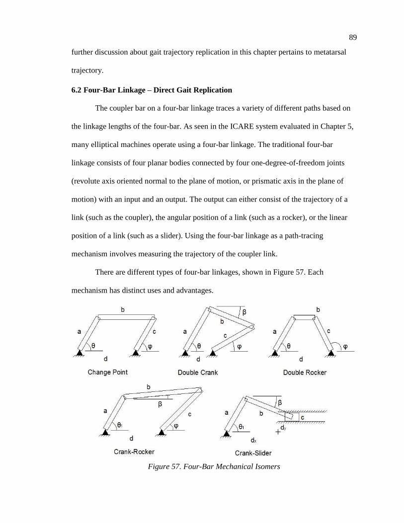
89
further discussion about gait trajectory replication in this chapter pertains to metatarsal
trajectory.
6.2 Four-Bar Linkage – Direct Gait Replication
The coupler bar on a four-bar linkage traces a variety of different paths based on
the linkage lengths of the four-bar. As seen in the ICARE system evaluated in Chapter 5,
many elliptical machines operate using a four-bar linkage. The traditional four-bar
linkage consists of four planar bodies connected by four one-degree-of-freedom joints
(revolute axis oriented normal to the plane of motion, or prismatic axis in the plane of
motion) with an input and an output. The output can either consist of the trajectory of a
link (such as the coupler), the angular position of a link (such as a rocker), or the linear
position of a link (such as a slider). Using the four-bar linkage as a path-tracing
mechanism involves measuring the trajectory of the coupler link.
There are different types of four-bar linkages, shown in Figure 57. Each
mechanism has distinct uses and advantages.
Figure 57. Four-Bar Mechanical Isomers

90
The Grashof existence conditions help determine what linkages are possible given
set link lengths [104-105]. The Grashof conditions use trigonometry to determine what
the link lengths must be to form a mechanism. For these equations, link L refers to the
longest link, link S refers to the shortest link, and links P and Q refer to the intermediate
links. The Grashof existence conditions are shown in Table 15. Note that the existence
condition for the crank-slider mechanism was also included in Table 15.
Table 15. Grashof Existence Condition for Four-Bar Linkages
Existence Condition Shortest Link (S) Mechanism Constructed
𝐿 + 𝑆 < 𝑃 + 𝑄 Ground Double-Crank
𝐿 + 𝑆 < 𝑃 + 𝑄 Crank Rocker-Crank
𝐿 + 𝑆 < 𝑃 + 𝑄 Coupler Double-Rocker
𝐿 + 𝑆 = 𝑃 + 𝑄 Any Change Point
𝐿 + 𝑆 > 𝑃 + 𝑄 Any Double Rocker
𝑏 − 𝑎 ≥ 𝑑𝑦 Crank Crank-Slider
One four-bar configuration is the double-crank (also known as the drag-link
mechanism). This design consists of two links connected to the ground through revolute
joints, both of which complete full rotations. Given uniform, constant angular velocity
from one of the cranks, the mechanism can output non-uniform angular velocity. A
trajectory traced by the output crank will always be a circle. For this reason, it was
excluded from consideration.
A specialized case of the double-crank is the change point configuration. A
change point mechanism is capable of fully rotating to a point where all four links
become collinear. As stated earlier, none of the double crank mechanisms were
considered for gait replication, so the change point configuration was discarded.
91
Another four-bar configuration is the double-rocker. This mechanism is
characterized by two links connected to the ground through revolute joints, both of which
oscillate between fixed angular positions as the coupler makes full rotations between
them. Without directly powering the coupler, this mechanism would be difficult to
control, and was excluded from consideration.
Another realization of a four-bar linkage is the crank-slider. In this, the
mechanism converts between linear, translational motion and angular, rotational motion.
The slider follows a predictable, oscillating trajectory based on the length of the crank
and the ground link vertical offset (labeled L4,x in Figure 57). Each point on the coupler
traces a closed, convex, non-circular path. Since the goal of this new mechanism is to
produce a gait-like trajectory that improves on the existing elliptical trajectories, this
mechanism was ruled out as a viable candidate.
The crank-rocker four-bar linkage converts the full, circular rotation of the crank
into an oscillating, finite angular movement of the rocker. Similar to the crank-slider, the
rocker arm experiences periodic, predictable oscillations. The coupler on the four-bar
linkage traces a variety of paths, such as the ones generated in Figure 58. Each coupler
trajectory forms a closed loop, but they vary between convex curves, self-intersecting
curves, and many other shapes. For this reason, it is much easier to consult an atlas of
four-bar linkages, such as the one produced by Hrones and Nelson [106]. After
consulting this atlas, none of the reviewed curves closely resembled the path presented in
Figure 35. If a sixth-order curve could be fit to the metatarsal trajectory path, then the
four-bar likely could be synthesized.

92
Figure 58. Sample Coupler Trajectories [106]
6.2.1 Development of Four-Bar Linkage Mathematical Model
The rocker-crank mechanism shown in Figure 57 is a one degree-of-freedom
mechanism. Each link can be represented by a vector. Since the four-bar linkage forms a
closed object, all of the vectors must sum to zero. From this knowledge, each vector was
broken into X and Y Cartesian components using the link length and the rotation angle.
The resulting summation is given by
𝑎 cos 𝜃 + 𝑏 cos𝛼 − 𝑐 cos𝜑 − 𝑑 = 0
𝑎 sin 𝜃 + 𝑏 sin 𝛼 − 𝑐 sin𝜑 = 0
Equation 6-1. Parametric Equations of Four-Bar Linkage Positions
where
a is the length of the crank,
b is the length of the coupler,
c is the length of the rocker arm,

93
d is the length of the ground link, which is the distance between the fixed
pivot on the crank and the fixed pivot on the rocker
θ is the angle between the crank and the ground link
α is the angle between the coupler and the ground link
φ is the angle between the rocker arm and the ground link
Note that all angles are measured counterclockwise from the ground link (which
is assumed to be horizontal for simplicity. Ground rotation can be easily adjusted at a
later time using a rotation of coordinate axes). From Equation 6-1, it is possible to derive
Freudenstein’s equation [107], which is given by
𝑅1 cos(𝜃) − 𝑅2 cos(𝜑) + 𝑅3 = cos(𝜃 − 𝜑)
Equation 6-2. Freudenstein’s Equation [107]
where
𝑅1 =𝑑
𝑐
𝑅2 =𝑑
𝑎
𝑅3 =𝑎2 + 𝑐2 + 𝑑2 − 𝑏2
2𝑎𝑐
Freudenstein’s equation can be used to determine the relationship between the
crank rotation angle and the rocker angle. Knowing the positions of both the crank and
rocker, the coupler position can be determined.
There are several methods available to optimize mechanism paths. The Burmester
method utilizes five points to calculate the trajectory of a coupler curve of a four-bar
configuration that passes through each point [108]. Initial efforts in using this method
indicated a substantially large mechanism would be generated, forming a curve that
extended far beyond the desired extents of the metatarsal curve.

94
Often, genetic algorithms and evolutionary methods are used to solve four-bar
linkage problems due to the complexity of the calculations involved in determining the
coupler position with respect to time [109-111]. Other algorithms have been implemented
through use of specialized MATLAB optimization functions [111-114].
6.2.2 Conclusions
The four-bar linkage as a method of fully replicating the gait path was not pursued
for this project. The gait path is a parametric function that involves both timing and
position. Seeking a four-bar linkage to approximate the path of the foot during gait would
require precise and variable control of the rotation of the machine to compensate for the
timing and position control.
Also, according to the second design goal, the mechanism must be adjustable. To
have perfect adjustment would require precise adjustment of each link to form a scaled
mechanism producing a scaled coupler output. Independent adjustments of four linkages
would be cumbersome and difficult, and may be prone to scaling error. In some
configurations of the four-bar linkage, it is possible to have minimal changes in trajectory
shape by scaling only one component, as seen in the crank redesign of Chapter 5.
However, the goal of this project was to develop a non-elliptical gait-like trajectory, and
utilizing a configuration similar to the one seen on the ICARE would not provide
significant benefits. Thus, the four-bar linkage as a method of fully replicating the foot’s
motion was not pursued.
6.3 Pantograph – Direct Gait Replication
Pantographs rely on geometrical constraints of similar triangles or parallelograms
to produce similar motions at different points on a linkage. One frame of a pantograph is

95
shown in Figure 59. The pantograph is fixed at point A, the lateral input movement
occurs at point O, and the output motion occurs at point C.
Figure 59. Single Pantograph Frame
Links AB, BC, CD, and DA all have the same length, forming a rhombus.
Isosceles triangle ABC and ADC each pass through motor point O. When the pantograph
frame is stretched from ABCD to AB’C’D’, the distance AO’ changes. By similarity of
triangles, lengths AO’ and O’C’ both expand at the same rate. This allows fixed
movements of point O or C to produce scaled movement across the pane. Since
pantographs rely on similarity of shape for all of the panes, this produces greatly scaled
motion based on the input motion. Two separate pantograph mechanisms were
considered for replicating gait motion.
6.3.1 Pantograph Realization #1
In one design, two long beams connect with two shorter beams to create a scaling
mechanism, as shown in Figure 60. Triangles ABC and ADF are similar triangles. Point
A is rigidly attached to the ground, and point F is attached to a foot pedal. Point C is
attached to a pin that would follow the reference gait path. A mechanism would be
constructed to power a pin through a gait-like trajectory. Through this motion, the pin’s
rigid connection with point C would control the shape of the pantograph trajectory.

96
Figure 60. Pantograph Path-Tracing Mechanism: Design 1
While this mechanism would be a simplistic method of accurately tracing the gait
trajectory, scaling would be difficult. In order to have exact path scaling, the triangular
symmetry must be maintained. To do this, points A, C, and F must lie along a straight
line. A motor would have to change link lengths so that the geometric similarities of the
triangles ABC and CEF remained. Also, the size of triangle ADF would be fairly
cumbersome in order to achieve a scaling between 8 and 40 in. This would make using
and mounting the machine difficult.

97
6.3.2 Pantograph Realization #2
A telescoping pantograph would extend outward, as shown in Figure 61. Again,
point A would be rigidly attached to the ground, and point C would trace the gait path
similar to the design shown in Figure 60. The foot pedal would be located at point C. In
order to scale, point C would be constrained to a different location along the axis of the
pantograph.
Figure 61. Pantograph Path-Tracing Mechanism: Design 2
This mechanism is significantly more compact than the one shown in Figure 60.
Also, scaling on this mechanism simply requires moving along the pantograph’s central
axis. Constraining point C to a position on the axis would be difficult, however. In order
to have accurate scaling, point C must move laterally with the position of the point
directly above and below it on the pantograph. One solution would be to pin C to
different hinge joints of the pantograph, but this leaves for sparse, discrete scaling points.

98
Another issue with the scissoring joints of this mechanism is that it poses a
potential pinch risk. For a device intended to be used with children, having dangerous,
pinching joints would cause serious concern for users of the device and could damage the
machine. This would require shielding, and would produce a rather bulky enclosure.
This pantograph machine is constrained only to move along one plane. With large
loads transmitted through the system from point C to point B, this likely would cause
some twisting of the pantograph rods. This would need to be minimized to prevent
damage to the system.
6.3.3 Assessment of Pantograph Feasibility
The pantograph mechanism has been proven to be a potent mechanism, and has
implications in art [115], with extendable arms [116], minimally-invasive surgical robots
[117], and other applications. Each of these applications, however, involved low-load
situations, and the extension of the pantograph was much slower than would be needed
for a gait therapy robot.
Because of the loading conditions required on a gait machine during operation,
the difficulty in scaling, the safety concerns of using this for pediatric patients, and
concerns over the machine jamming or damaging itself during operation, the pantograph
device was not pursued.
6.4 Foundations of Parametric Gait Modeling
In direct path modeling, the trajectory of the metatarsal from Figure 35 was
recreated using known mechanisms. For parametric gait modeling, the gait path is broken
up into separate, independent coordinate pairs based on the time, similar to the parametric
mathematical modeling that was performed in Section 4.2.2.

99
Parametrization in Cartesian coordinates is difficult to scale. Independent
mechanisms controlling the X and Y positions of the foot pedal are required, and each
mechanism must be scaled about a defined point. This requires two adjustable, scalable
inputs for the system.
As an alternative to Cartesian parametrization, polar parametrization only requires
one scalable, radial input and one fixed, angular input. Due to the dimensionless nature of
the angle, no scaling is necessary. However, the origin of the polar parametrization is
important to controlling the trajectory of the foot, as shown by the vastly different curves
presented in Section 4.2.2.
6.4.1 Leading Foot Parametric Solution
To match the design goals presented in Section 6.1, the mechanism must not be
too difficult to scale, or become excessively large when scaled. For example, consider a
crank-slider system with an origin consistent with the parametric origin located 1.5 stride
lengths in front or back of the foot, as shown in Figure 62. Note that a metatarsal
trajectory curve is plotted on top of the sliding foot plate in this figure.
Figure 62. Sample Radial Parametrization of Metatarsal Trajectory
This system would require the radial and angular positions seen in Figure 26 or
27, which generates very smooth, easily replicable trajectories. However, if a 40-in. long

100
stride length were to be obtained by this mechanism, the scaling for those particular
curves would require at least 80 in. of space between the origin of the rotating bar and the
rear of the metatarsal trajectory according to these design parameters. Note that the
distance between the rotating bar and the rear of the trajectory does not account for the
length of the foot pedal behind the metatarsal. This distance was undesirable, and creates
an excessive mechanism footprint. Moving the origin point closer to the metatarsal
trajectory does decrease the required distance, but the change in angle of the bar during
one cycle increases.
6.4.2 Hip Origin Parametric Solution
As discussed in Section 4.2.2 and references 92 and 93, the toe trajectory has been
modeled as tracing an arc trajectory about the hip. Using the toe trajectory in Figure 30, a
device could be designed to mimic the toe trajectory while rotating about the hip. For
example, one realization involves attaching a foot pedal to an actuated, adjustable linkage
that lifts the foot during stride and lowers during gait (similar to Figure 30). The cadence
of this motion could be controlled with a four-bar linkage. This idea is shown in Figure
63.

101
Figure 63. Scalable Device with Polar Origin at Hip
While this idea is feasible, it would require novel design to make the stride
adjustment between 8 and 40 in. This design shows some promise, as it is accessible from
the rear for body weight support mechanisms. This device would be wider than
traditional gait therapy mechanisms, and may not fit through doorways. Due to time
restrictions, this idea was not pursued.
6.4.3 Parametrization to a Point on the Gait Path
A mechanism with the origin located on the gait path would be conceptually
simple. This would minimize the footprint of the mechanism because the length of the
system utilized by the user would be determined by two factors: the maximum stride
length and the length of the foot pedal. Having an origin located on the gait path would
also make placement of the handle bars easier. However, tracing the metatarsal trajectory
with polar coordinates results in radial-angular curves like the ones seen in Figure 25.
The discontinuity in the angular data is associated with high angular accelerations, which
are unrealistic.

102
Using the mathematical-average metatarsal and foot angular data from Chapter 4,
it is possible to construct an equation that describes the gait trajectory at each location
along the foot. This equation is given by
𝑉𝑝⃗⃗ ⃗ = 𝑉𝑚⃗⃗ ⃗⃗ + 𝐿𝑝−𝑚 ∗ ⟨sin (𝐴𝑓), cos (𝐴𝑓)⟩
Equation 6-3. Foot Point Gait Path Determination
where 𝑉𝑝⃗⃗ ⃗ is the set of X,Y vector coordinates defining the gait path of the chosen location
of the foot, 𝑉𝑚⃗⃗ ⃗⃗ is the set of X,Y vector coordinates defining the metatarsal gait path,
𝐿𝑝−𝑚 is the distance from the metatarsal to the chosen foot location (normalized by the
stride length), and 𝐴𝑓 is the angle defining the foot angle during gait.
Equation 6-4 can be used to cause the swing and stance trajectories to be tangent
at 0, resulting in the angular and radial position parametrizations shown in Figures 64 and
65. With this new trajectory, a radial parametric equation to be established at the center
point of the stride. It was determined that when 𝐿𝑝−𝑚 = −0.1 (at a point in front of the
foot located 0.1 stride lengths ahead of the metatarsal), the gait path resembled that of
Figure 64.
Figure 64. Projected Foot Path with Minimized Trajectory Height at Center Stride
Direction of Travel

103
Figure 65. Raw Radial and Angular Traces of Mathematically Predicted Point
Both the angular and radial position of Figure 65 show discontinuity at the start
and end of the stride, and the midstride also experiences a discontinuity. To compensate
for both of these, the radial position was allowed to become negative for half of the cycle,
and the angular position was forced to be zero directly at and around the discontinuities.
The resulting parametrization is shown in Figure 66.
Figure 66. Smoothed Mathematically-Predicted Gait Path Radial Parametrization

104
As shown above, it was possible to find a point on the foot that follows a
trajectory that tangentially intersects itself at the stride midpoint. However, the foot does
not pivot about this point. Modeling the stride about this point requires a forced lift of the
heel to operate, or the person would have to lift their foot off of the ground and assume
normal heel trajectory. While this would make the gait replication process more difficult,
it was considered to be the best method for reproducing gait trajectories.
6.5 Scotch Yoke-Cam – Parametrized Gait Replication
The gait path shown in Figure 64 is promising when considered for parametric
modeling. One realization of this mechanism is a sliding foot carriage operating on a
rotating beam propelled by a Scotch yoke mechanism (double-slider). The beam angular
movement could be controlled by a crank rotating at a constant speed. This design is
shown in Figure 67. The rotation of Link B drives the forward and backward movement
of the foot pedal, Link D. Adjustment to Link B changes the stride length. Rotation of
Link E causes Link A to pivot. In order to center the stride over the pivot point on Link
A, the length of Link C would have to be adjusted.
Figure 67. Scotch Yoke Realization of Parametric Modeling

105
This design showed potential as a solution. The sliding Link C along the rail
would pose some frictional issues, and would not be as efficient as possible in that
regard. Also, the motor would require a special control to attempt to mimic the timing of
the radial curve, which is not perfectly sinusoidal.
6.6 Rocker-Cam – Parametric Gait Replication
Building on the idea of the Scotch yoke mechanism described in Figure 67, a
rocker-crank mechanism was proposed to propel the foot through the movements. The
rocker would be connected to the forward-backward movement of the foot pedal, and this
would be scaled by increasing and decreasing the height of the connection to the rocker,
which scales the output distance linearly. The benefit of using a rocker-crank mechanism
include (1) fine-tuned design of the four-bar linkage would allow for a rocker movement
more consistent with the foot pedal motion, (2) easier scaling, (3) more efficient transfer
of load, and (4) more stable application of load than using a pin-in-slot configuration.
Using a crank-rocker to power the foot pedal requires more linkages than a Scotch
yoke mechanism. The proposed rocker-cam mechanism is shown in Figure 68. The
revolution of the crank (Link A) causes the rocker (Link C) to pivot, which (in turn)
slides the foot pedal (Link E) along the rail (Link F). The rotation of the cam (Link G) is
in phase with the rotation of the crank, and drives the pivoting motion of the rail.
Figure 68. Rocker-Cam Parametric Gait Replication

106
One problem with the rocker-cam configuration shown in Figure 68 is that the
scaling is not linear. Since the connection between the rocker and the foot pedal (Link D)
is rigid, moving Link D along the rocker will actually cause the foot pedal position to
move slightly. This would have to be compensated for in the final design.
Another issue with the proposed rocker-cam configuration is that the mechanism
is difficult to power under the user’s will. At the forward and backward positions, the
mechanism is difficult to self-power. The machine may require some assistance in
moving the feet through this locking position. A flywheel or attached motor would help.
6.7 Conclusions and Chosen Mechanism
While several viable options were considered for realizing the planar gait path
replication problem, one option stood out the most as fulfilling the design goal
requirements shown in Section 6.1. Direct gait path replication methods showed a strong
ability to accurately replicate the trajectory, but did not show acceptable timing control,
maximum forces, and mechanism footprint. On the other hand, parametric gait path
replication methods showed an ability to precisely control timing and mechanism
footprint, but were significantly more complicated and risked de-coupling the radial and
angular motions of the foot. It was decided that the rocker-cam design shown in Section
6.6 would be pursued for gait path replication.

107
CHAPTER 7 – ITERATION I
The rocker-cam mechanism described in Section 6.6 was chosen to replicate the
trajectory of a foot point located 0.1 stride lengths in front of the metatarsal. The
mechanism was refined, and efforts were made to ensure linear scaling, proper timing,
and accuracy of trajectory. A method of integrating heel lift was incorporated into the
design in order to facilitate the foot angle changes. It should be noted that due to time
restrictions, a full system simulation was not conducted.
7.1 Overall Design
Three separate systems are needed to fully replicate the foot motion:
The four-bar linkage driving the foot forward-backward motion along the
rail
The cam rotation driving the rail angular position
The mechanism for heel lift to replicate foot angle during gait
The sliding mechanism attached to the rocker to determine path scaling will be
subject to slight vertical motions during the movement of the rocker. One method of
compensating for this nonlinearity is to constrain a bar to only move longitudinally. This
bar would have a sliding connection with the rocker, and the height of this bar off of the
ground determines the overall scaling. Movement of this bar would cause a pinion to
rotate, generating a rotational motion. Converting the motion into rotational distance
allows for gearing to occur, which minimizes the required size of the four-bar linkage.
The rotational motion is converted back into translation along the rail at the central hub.
The mechanism for heel lift must be constant along the length of the rail,
remaining unchanged with varying stride lengths. One method of lifting the heel involves

108
a secondary rail that lifts up the rear of the foot carriage. This could be accomplished
through the use of cams and a rail. The proposed concept of the full system is shown in
Figure 69.
Figure 69. Proposed Mechanism Control Systems
7.2 Rocker Optimization
The four-bar linkage needs to be designed so that the rotation of the rocker
matches the timing of the foot longitudinal motion seen in Figure 66. Several
considerations go into the design of a four-bar linkage:
The transmission angle (the angle between the coupler and the rocker) is
integral to determining the mechanism efficiency. Transmission angles
near 90 degrees minimize power losses.
The coupler and rocker bar cannot encounter any toggle positions (points
where the coupler and rocker are parallel); this may cause the mechanism
to experience unpredictable movements and/or catastrophic failure due to
shock loading.

109
The four-bar linkages must not contact anything during their rotations or
else this could cause catastrophic failure or seizure of the machine.
The four-bar link lengths must abide by the rocker-crank Grashof
condition given by Table 15.
Special conditions are applied to this mechanism to match the design goals in
Section 6.1:
The mechanism must not have a large footprint.
A simple four-bar mechanism was chosen as a starting point for the design. A
crank length of 8 in. was selected. The transmission angle was chosen to vary a total of
60 degrees, deviating 30 degrees from perpendicular in either direction. From these
parameters, the rocker length was chosen to be 16 in., and the coupler length was chosen
to be 14 in. The resulting configuration is shown in Figure 70.
Figure 70. Initial Four-Bar Linkage Configuration for Analysis

110
An iterative MATLAB program was written to perform a nonlinear optimization
on the design of the four-bar linkage. From Freudenstein’s equation (Equation 6-2), it is
possible to derive an equation for the rocker angle:
𝜑 =cos−1(𝑅1 cos 𝜃 + 𝑅3)
𝐴3− 𝜓
Equation 7-1. Rocker Angle (Derived from Freudenstein’s Equation)
where each of the dimensionless simplification variables are explained below:
𝐴3 = √(cos 𝜃 + 𝑅2)2 + sin2𝜃
𝜓 = tan−1(− sin 𝜃
cos 𝜃 + 𝑅2)
𝑅1 =𝑑
𝑐
𝑅2 =𝑑
𝑎
𝑅3 =𝑎2 + 𝑐2 + 𝑑2 − 𝑏2
2𝑎𝑐
Each of the mechanism parameters is explained below:
a is the length of the crank,
b is the length of the coupler,
c is the length of the rocker arm,
d is the length of the ground link, which is the distance between the fixed
pivot on the crank and the fixed pivot on the rocker
θ is the angle between the crank and the ground link
φ is the angle between the rocker arm and the ground link
To determine the optimal four-bar configuration to match the rocker angle
equation from Equation 7-1, a nonlinear optimization method was used. In random
stochastic optimization methods (such as genetic algorithms or information search

111
methods), random variable changes are assessed to determine a minimizing vector
direction [118]. For gradient based methods (such as steepest descent or Newton’s
method), the direction of descent is determined and iteratively utilized to directly find a
minimum [119]. By nature, gradient-based methods converge significantly faster than
stochastic optimization methods when the search space is “well behaved.”
With this problem, the four-bar linkage is limited by the Grashof existence
condition for the crank-rocker mechanism provided in Table 15. This also means that the
crank must be the smallest link in the mechanism. These constraints can be easily
implemented into the gradient-based solution, and thus, the steepest descent method was
chosen for optimization.
First of all, a time-dependent least-squares optimization was implemented that
summed the squares of the errors between the produced rocker angle and the ideal rocker
angle. The optimized function was given by
𝑓(𝑥 ) = ∑(𝑅(𝑥 )𝑖 − 𝐹𝑆𝑖)2
𝑁
𝑖=0
Equation 7-2. Optimization Function (Least-Squares Error)
where N is total number of points considered for the optimization; 𝑅(𝑥 )𝑖 is the rocker
angle given by a particular time in the cycle i; 𝑥 is the vector containing the lengths of the
crank, coupler, rocker, and ground linkages, respectively; and 𝐹𝑆𝑖 is the Fourier series
average function value at that time in the cycle. Here, 𝑅(𝑥 )𝑖 is given by Equation 7-1
based on the timing of the crank.
The equation for each iteration of a gradient-based optimization method is given
by [120-121]
𝑥𝑖+1⃗⃗ ⃗⃗ ⃗⃗ ⃗ = 𝑥𝑖⃗⃗ ⃗ − 𝛼𝑃𝑖⃗⃗

112
Equation 7-3. Iterative Equation for Optimization Problem
where 𝑥𝑖+1⃗⃗ ⃗⃗ ⃗⃗ ⃗ is the vector set of the lengths of the four linkages in the next iteration, 𝑥𝑖⃗⃗ ⃗ is
the vector set of current linkages, 𝑃𝑖⃗⃗ is the vector defining the minimizing direction for
this iteration, and 𝛼 is the scalar applied to the equation to define the magnitude of the
minimizing direction to ensure adequate minimization. For the steepest descent method,
the minimization direction is given by
𝑃𝑖⃗⃗ = ∆𝑅(𝑥𝑖⃗⃗ ⃗) = 𝐉T ∗ (𝑅(𝑥 )𝑖 − 𝐹𝑆𝑖)
Equation 7-4. Minimizing Direction Vector for Steepest Descent
where 𝐉T is the transpose of the Jacobian matrix of Equation 7-1 with respect to the
linkage lengths, 𝑥 . Using the steepest descent method of nonlinear optimization, the
initial conditions were input and the program was run to completion twice, obtaining two
separate four-bar linkage designs. The initial conditions and the result of both program
iterations are compared to the desired rocker trajectory in Figure 71. The full MATLAB
program code is found in Appendix C. The optimized four-bar linkage configurations are
shown in Figures 72 and 73.

113
Figure 71. Nonlinear Optimization Comparison of Four-Bar Rocker Angles
Figure 72. Nonlinear Optimization Configuration I

114
Figure 73. Nonlinear Optimization Configuration II
7.2.1 Discussion and Four-Bar Selection
Comparing the rocker angles given in Figure 71, the original, non-optimized
rocker angle curve generated by the mechanism in Figure 70 appears to approximate the
ideal curve well. Using a least-squares method of determining error, the 200-point curve
had an error value of 5.49, as compared to the optimized curve’s error value of 1.72. A
least-squares curve does not fully explain the closeness of fit, however. While it does
mathematically show that the curve better follows the shape of the ideal rocker angle, the
optimized curve does not show that it is a better fit for driving human foot motion. The
non-optimized rocker appears to be smoother and does not have as sharp of a transition
between forward and backward motion, which would reduce the stresses imparted on the
system by minimizing the accelerations. Efforts to force smoothness on the optimization
code would result in four-bar configurations that are less accurate than the initial

115
configuration. For these reasons, the non-optimized four-bar linkage from Figure 70 was
selected for use with the gait therapy device.
7.3 Cam Design
A trajectory can be explicitly written as a parametrized set of coordinates that are
functions of time. Implicitly, each coordinate is dependent on the other coordinate. Small
changes in the timing of one coordinate can drastically affect the overall trajectory,
producing a highly erroneous shape. From Section 7.2, the chosen four-bar linkage
results in a rocker angle profile that differs from the desired rocker motion. In order to
have a working parametrization, the crank angle (and the position of the cam, which is
integrally linked to the crank angle) must be adjusted. Using a lookup algorithm to
determine when the corresponding time is for each crank rotation position, the difference
between the actual time and the required crank position can be measured. This timing lag
is shown in Figure 74. This can be used to adjust the rail angle for the new design.
Figure 74. Timing Lag for Chosen Four-Bar Linkage

116
Cam placement along the rail affects the cam acceleration, cam displacement, and
cam loading. Two issues arise when considering cam placement. (1) The farther away
from the pivot point the cam is, the larger the cam height variability, higher necessary
velocities, and larger accelerations by conversion of radial to Cartesian coordinates. This
equates to higher forces transmitted through the cam. (2) The closer to the pivot point the
cam is, the longer the cantilever when the foot pedal is at its maximum stride length.
Longer cantilevers mean that the rail is subject to more instability, as the user feels more
movement in the system further from the pivot point.
Since the maximum stride length was ideally chosen to be 40 in., the cam position
was picked to be half of that – 10 in. away from the pivot point in either direction.
Having dual cams allows for the rail to be supported fully as the foot travels through the
trajectory. Using the cam placement and the timing lag determined from Figure 74, the
cam vertical profile was generated. The cam vertical profile is shown in Figure 75.
Figure 75. Time-Adjusted Cam Height Profile

117
Ideally, the cam would rotate at approximately 1 rev/s (2π rad/s). The cam
acceleration was determined using trapezoidal numerical integration. Unfortunately,
placing the cam at 10 in. away from the pivot line meant that the cam experienced
extremely high accelerations at this rotation speed. It was decided that accelerations
should be limited to approximately the gravitational constant, which is recommended to
maintain sufficient contact between the cam and the follower [122]. A 330 in./s2
maximum acceleration was manually applied to the profile. Both the ideal and
acceleration-limited profiles are shown in Figure 76. Note that the accelerations were
zero outside of the bounds of this graph. Using the second derivative of the cam height
position from Figure 75, the acceleration-limited cam displacement was compared to the
ideal cam displacement. The resulting profile is shown in Figure 77.
Figure 76. Cam Acceleration Profile

118
Figure 77. Cam Displacement Profile
While the acceleration-limited cam displacement did not result in the desired
angular displacements, it was enough to register a significant rail movement. Using the
acceleration-limited cam displacement profile, a cam was generated. The full cam shape
is shown in Figure 78. The projected foot path generated by using the four-bar linkage
from Figure 70 paired with the cam shape from Figure 78 is shown in Figure 79. Note
that the two trajectories are similar, though the mechanical trajectory shows obvious
narrowing.

119
Figure 78. Iteration I Cam Shape
Figure 79. Mechanical vs. Desired Gait Trajectories
The purpose of powering the toe through a gait-like trajectory is to attempt to
simulate walking. While the mechanical gait-like trajectory was a reduced form of the
desired trajectory, it would still displace the foot from the ground, which may be enough
to trigger a gait-like motion. Testing will determine the effectiveness.

120
7.4 Foot Angle
The foot angle was decided to be fixed by lifting the rear of the foot carriage. To
accomplish this, a rail underneath the foot carriage rose and engaged a wheel on the
underside of the foot carriage, causing the carriage to rotate upward. The distance needed
for this lift depended on the placement of the wheel relative to the pivot point. The farther
away from the pivot point that the wheel was mounted, the larger the distance to lift the
foot. At the same time, the closer to the pivot point, the more difficult to constrain the
foot pedal lateral and rotational movements.
A 5-in. diameter wheel was mounted to the bottom of the foot pedal 6 in. away
from the pivot point, resulting in the geometry shown in Figure 80.
Figure 80. Foot Pedal Model
Based on the foot pedal geometry, the foot angle correlated with the rail lift
according to the equation:
𝑏 = 𝐿 tan𝛼
Equation 7-5. Foot Angle Relationship with Rail Lift

121
where b is the height of the heel lift. Applying this correction to the foot angle, the profile
for the heel cam was generated. This was adjusted according to the time correction shown
in Figure 74, and the resulting heel cam profile is shown in Figure 81.
Figure 81. Ideal Heel Lift Height Profile
Acceleration was determined using the displacement profile from. The
accelerations of this cam were fairly large for the chosen profile. Using the same
maximum acceleration limit set for the rail angle cams (330 in./s2), a new acceleration
profile was generated. The two acceleration profiles are compared in Figure 82. Note that
the acceleration is considered zero outside of the bounds of this figure. The acceleration-
limited profile was manually generated, and had to attempt to match the ideal
acceleration curve. At the same time, double integration of the acceleration curve has to
result in a net zero displacement so that the cycle is maintained. The resulting lift
acceleration and displacement curves are shown in Figures 82and 83, respectively.

122
Figure 82. Acceleration Comparison between Ideal and Acceleration-Limited Profiles
Figure 83. Heel Lift Displacement Comparison
The heel lift for the acceleration-limited displacement profile was significantly
lower than the target heel lift displacement profile. The cam profile generated by the heel
lift curve is shown in Figure 84. The disparity in heel heights in Figure 83 causes a

123
deficiency in the foot angle, as shown in Figure 85. While the foot angle was
significantly less severe for the acceleration-limited cam profile, it was hoped that
minimal pressure on the heel during toe-off would assist the users in manually passing
through the full foot motion.
Figure 84. Foot Angle Cam Shape
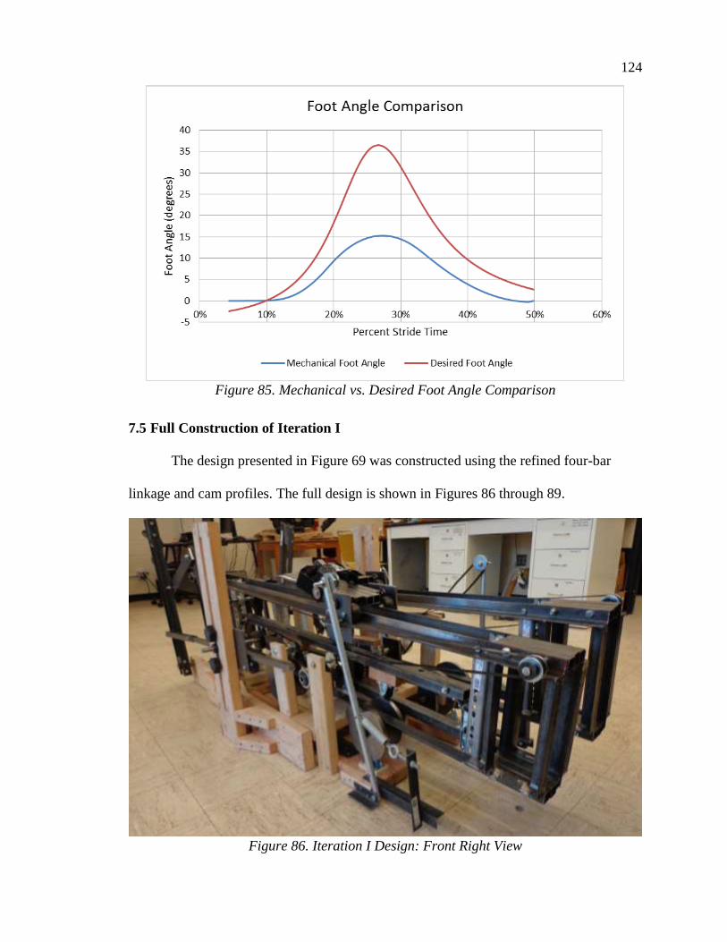
124
Figure 85. Mechanical vs. Desired Foot Angle Comparison
7.5 Full Construction of Iteration I
The design presented in Figure 69 was constructed using the refined four-bar
linkage and cam profiles. The full design is shown in Figures 86 through 89.
Figure 86. Iteration I Design: Front Right View
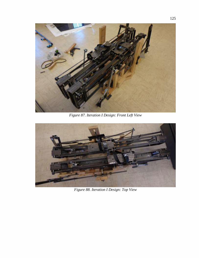
125
Figure 87. Iteration I Design: Front Left View
Figure 88. Iteration I Design: Top View

126
Figure 89. Iteration I Design: Rear Left View
7.6 Iteration I Performance
The mechanism, as constructed, was unable to move under human input. As
constructed, the resistances in the system were too great to overcome. When individual
systems were powered by hand, they showed marked resistance and movement was
choppy.
The inability of the machine to operate naturally means that the foot angle control
system was not tested. To minimize the power requirements of the system, analysis on
the mechanism was conducted without the foot angle control system in place.
The rail angle control system was overconstrained due to the presence of dual
cams and the rail pivoting point. In order for the cams to rotate, the rail had to flex.
Applying some clearance between the mechanism and one of the cams alleviated this

127
constraint. However, the sharp accelerations of the cams made rotation very difficult, and
the rail would shake with each rotation.
The foot pedal longitudinal control system was inefficient. As designed in Figure
69, the belt that carried the longitudinal load around the rail had to have tensioners
attached to it to maintain contact with the bottom, rotating gear. This caused significant
friction in the system, and made the forward and backward motion of the foot difficult.
The vertically-constrained bar attached to the rocker experienced large moments, and this
caused the mechanism constraining the bar to crack during use. Also, the rack and pinion
had difficulties with jamming due to the poor constraints, and made a considerable
amount of noise during operation.
Overall, the system was arrested and could not operate under motorized
assistance, let alone purely human control. Motion was choppy and loud. The rail was not
convenient to use, as it was shaky and tall. The arrested behavior was blamed on poor
tolerancing, misaligned shafts, heavy components, rail weight, and large cam
accelerations. The performance of Iteration I, compared to the mechanism design goals
outlined in Section 6.1, is summarized in Table 16.

128
Table 16. Iteration I Performance vs. Design Goals
Design Goal Description Iteration I Performance
Gait-Like
Trajectory
Traced path must resemble
average gait curve
Traced path was similar to gait path,
including foot angle
Scalable Must accommodate
pediatric and adult patients
Mechanism was scalable for stride
lengths, but scaling control fractured
Practical Usable in small facilities One motor controlled all functions,
easy to manage.
Adjustable Accommodate specific
impairments
Adjustable for varying stride
lengths, adjustment was simple
Cost-Effective - - Comparably priced due to cheap
components
Small Footprint - - Heavy, but small enough to be
functional in a rehabilitation setting
Motorized Able to be motorized Mechanism was arrested, could not
be powered at all
Backdrivable Able to be driven by
human power Impossible to backdrive
Ergonomic Easy and comfortable to
mount and operate
Not comfortable, sturdy, quiet, or
easily mounted

129
CHAPTER 8 – ITERATION II
Design Iteration I was considered a failure. Despite aiming to satisfy all the
design conditions of Section 6.1, the inability of the mechanism to move overshadowed
its design. As such, a new design was considered and created to replace Iteration I. It
should be noted that, similar to Iteration I, time restrictions prevented the construction
and evaluation through a full-system simulation.
8.1 Design Goals Revisited
The original design goals for this project were to design a machine that replicated
a gait-like trajectory with a scalable output. Ideally, the mechanism would also have a
small footprint, be cost-effective, adjustable, backdrivable, motorized, and ergonomic.
Iteration I attempted to tackle all of the design goals.
The gait-like trajectory for Iteration I was acceptable. However, the scaling
mechanism for Iteration I was overly complicated and caused the mechanism to break.
The constraints for the scaling mechanism would need to be adjusted on the new design.
Iteration I had an acceptable footprint. To improve the design, the height of the
foot pedals in the new design would need to be decreased to make mounting the machine
easier. Ideally, that would also equate with a significant weight decrease.
Iteration I was fairly cost-effective, proving that the design did not need to be
expensive in order to be constructed. More leniency on cost would be allotted to the next
design to utilize better components and improve the machining quality.
It was not possible to backdrive Iteration I. Further iterations utilizing similar
rocker-cam mechanisms to Iteration I would not be backdrivable either, and as such, that
design goal was omitted from consideration.

130
The rail would need to be significantly sturdier in the next design. For Iteration I,
the rail was large and cumbersome, and tended to sway noticeably when mounted. Also,
to decrease the operating noise, the cam shapes would need to be adjusted to lower the
acceleration limits.
Finally, in order to make it functional, methods to reduce the number of
tensioners needed and axles needed to operate the machine need to be implemented. For
Iteration I, there were four separate cam axles, one central axle, one crank axle, and
numerous tensioners to maintain tightness in the long stretches of belt and chain.
8.2 Complete Design
The full design for Iteration II is shown in Figures 90 and 91. This design
implemented many of the design changes needed as mentioned above. Overall, the
system showed improved power transmission, ergonomics, weight reduction, and
manufacturing difficulty, while showing slight increases in nonlinear scaling, reduction
of the accuracy of the full trajectory of the foot, and removal of the foot angle control
system. Individual changes to components and systems are discussed in the following
sections.
Figure 90. Conceptual Design of Iteration II

131
Figure 91. Component Model of Iteration II
8.3 Improved Scaling Mechanism
For Iteration I, the scaling mechanism consisted of a rack that was constrained to
slide forward and backward along a horizontal path with oscillation of the rocker. The
forces passing through the rocker loaded the machine past its stress limit, causing
cracking of the adjustable scaling component.
A simpler method of connecting the scaling bar to the rocker is through a sliding
block that is able to move up and down along the length of the rocker. To fix this block in
place, a pin was placed through one of many holes vertically spaced along the rocker and
into the block. While this did discretize the scaling, it also allowed for repeatable, precise
stride adjustments.
Rather than using a convoluted myriad of tensioners, pinions, and axles to connect
the rocker to the food pedal, it was decided to directly connect the two. A bar extended
from the pinned block down to the foot pedal, where it connected to the foot pedal with a
revolute joint. This significantly simplified the connection and minimized potential losses
due to power transmission. One issue with this setup is that the distance between the
carriage and the block changes depending on how high the connection is above the rail.

132
Also, the originally horizontal rocking motion created by the rocker now experienced
some vertical deflection which increased with increasing stride length. This introduced
nonlinearity into the scaling.
8.4 Redesigned Rail and Carriage
The rail design for Iteration I of the gait mechanism device utilized a tall, welded
rectangle with a homemade carriage riding along it. The rectangle provided space for the
foot angle-controlling rail to translate inside of it. While this option was inexpensive and
robust, it was wobbly in out-of-plane motions, tall, and cumbersome. The rail was
replaced with an off-the-shelf rail and linear motion carriage, as shown in Figure 92. This
configuration, while significantly more expensive than the rail and carriage used in
Iteration I, would provide more stability, less frictional losses, and weigh significantly
less. Also, the height of the rail was reduced from 12.44 in. to 1.18 in.
Figure 92. Off-The-Shelf Rail and Linear Motion Carriage
As stated in Section 8.3, the new scaling mechanism caused a change in distance
between the rocker and the carriage as the stride length was adjusted. To compensate for
that, the scaling mechanism was connected to a secondary carriage riding along the rail.

133
That carriage was connected to the foot pedal carriage through an adjustable link (screw).
The idea behind the adjustable link was that it would allow researchers to fine-tune the
location of the carriage to the correct position. This is important since the full foot
trajectory is scaled about the center point of the stride at the pivot point of the rail.
8.5 Cam Acceleration Limitations
The cam profile from Iteration I proved to be too severe. It was decided that the
profile would be further limited in acceleration to approximately 60% of the gravitational
acceleration, or 220 in./s2. The decision to use 60% of the original accelerations was
arbitrary, and due to the time constraints of the design, further optimization analysis was
impossible (but could still be done in the future). The resulting cam acceleration curve for
the Iteration II cam is compared to the Iteration I cam and the desired rail acceleration in
Figure 93. The resulting rail angular displacement is compared to Iteration I and the
desired displacement in Figure 94.

134
Figure 93. Cam Acceleration Comparison
Figure 94. Rail Angular Displacement Comparison

135
The limited-acceleration cam profile for Iteration II resulted in significantly
reduced rail angles. With peak rail angles of approximately 3.5 degrees, the user may feel
the force transmitted through the cam, but likely will not feel a significant change in rail
angle. There is a possibility this will trigger natural foot movements. Normal foot
movements may occur if the user lifts the heel during toe-off and lifts the toe during heel
strike.
8.6 Removal of Foot Angle Rail
In Iteration I, a mobile rail actuated with the bottom of the foot pedal to change
the foot pedal angle, causing the foot pedal to rotate. After review, it was the belief of the
Madonna researchers that this was unnecessary. During normal gait, the tendon
connecting the heel to the calf muscle pulls on the heel, causing the heel to rise during
toe-off. The foot then rotates about the knee joint, and at heel strike, the toe is oriented at
an incline to the horizontal. The rotation of the knee is the primary cause of the foot angle
following toe-off. Between the knee rotation and the natural heel lift, the foot may trace a
natural trajectory during gait without the extra assistance. Thus, it was advised that the
foot angle rail should be removed.
8.7 Motorization
Because the system is not backdrivable, the machine required a motor to operate.
Specifically, the motor was needed for assistance in overcoming the toggle points of the
four-bar linkage. Unlike Iteration I, which had six separate axles and multiple tensioners,
this design only had two axles. The simplest form of connecting them involved using a
single chain wrapped around the cam axle and the crank axle.

136
A motor was utilized to propel the foot and turn the cams to dictate foot angle.
The unloaded motor speed was 1,750 RPM, with a maximum voltage of 80 Volts. The
stall torque was 27 N-m, and the stall current was 7.6 Amps. To maximize the torque
output of the motor, the motor needed to run near 1,750 RPM when the machine was at
maximum speed. As stated earlier, the ideal speed for the machine was 1 rev/sec (or 60
RPM). Assuming the max speed occurs at 80% of the ideal stride time, the max RPM of
the machine would be expected to be 75 RPM. In order to get this scaling up near the
motor speed, the motor had to be scaled down by a factor of 23.33.
The smallest ANSI-40 steel sprocket sold by McMaster-Carr is a 9-tooth, 5/8-in.
bore sprocket. This sprocket was mounted onto the motor axle, and it interfaced with a
45-tooth, ANSI-40 sprocket on the power transmission axle. A 9-tooth, ANSI-40
sprocket on the power transmission axle interfaced with 35-tooth, ANSI-40 sprockets on
the cam axle and the crank axle. Overall, the gear ratio for this machine was 19.44. While
that was less than the desired gear ratio, a higher gear ratio would only be possible with a
third power transmission axle or larger sprockets on the cam and crank axles. The
resulting chain diagram for the machine is shown in Figure 95.
Figure 95. Initial Power Transmission Configuration

137
The contact angle is defined as the angle (measured from the center of a sprocket)
that the chain is in contact with the sprocket. Ideally, this angle would be at least 120
degrees, although it is possible to have lower contact angles at larger tooth numbers on a
sprocket [123,124]. Also, it was noticed during operation that the 9-tooth power
transmission sprocket was slipping against the chain, causing the system to jump over
that sprocket and not engage. To improve the contact angles of these sprockets and
tighten the chain into the sprockets, it was suggested that idler sprockets be mounted.
Two idler sprockets were attached to the system, and they helped to route the chain. One
idler sprocket was mounted on a fixed shaft that passed through the system laterally. The
other idler sprocket was mounted to a bolt so that the chain tension could be manually
adjusted. The resulting power transmission diagram is shown in Figure 96.
Figure 96. Chain-Tensioned Power Transmission Diagram
It was noted that the structure supporting the crank axle was deflecting
significantly during operation using the configuration shown in Figure 96. This was
attributed to the large forces transmitted through the chain during several peak locations
of the cam’s rotation. In order to prevent failure in the support structure for the crank
axle, the power transmission to the crank axle and to the cam axle must be separated.

138
Two 9-tooth, ANSI-40 sprockets were placed on the power transmission axle, and the
cam and crank engaged different sprockets. This decreased the force transmitted through
each chain. The resulting configuration is shown in Figure 97.
Figure 97. Dual-Chain Power Transmission System
8.8 Iteration II Construction
Iteration II was constructed, and the full mechanism was proven to be operational.
Initial testing showed that the machine was capable of handling 250-lb individuals and
propelling the feet without significant issues. The constructed Iteration II, as designed, is
shown in Figure 98. The constructed Iteration II with a new foot pedal is shown in Figure
99.

139
Figure 98. As-Designed Iteration II Assembly

140
Figure 99. Assembled Iteration II with New Foot Pedal

141
One major design change was implemented by the Madonna staff. While the
device had been designed to model the trajectory of a point on the foot just in front of the
toe (see Section 6.4), researchers at Madonna showed concern about the user being able
to lift the foot pedal naturally. As such, they requested that the pivot point be shifted from
the toe to a point near the metatarsal. No redesign work to the cam or four-bar linkage
was done, and the new foot pedal (shown in Figure 99) replaced the existing foot pedal
along with the change.
8.9 Preliminary Performance Evaluation
Early results from the testing of the Iteration II design show that the device did
not encourage a gait-like trajectory. Rather, the device appeared to operate more like a set
of skis, where the stance and swing phase followed nearly the same trajectory. On use of
the machine, it was noted that the device did not encourage the user to bend the knee or
flex the ankle joint anywhere near the proper positions. The foot angle was very flat for
most of the trajectory.
As per the opinion of the author after use, the timing of the stride did feel very
comfortable, and the anterior and posterior motions of the legs felt natural. This can be
accredited to the four-bar linkage selection.
While these are preliminary results, they warrant future work. More effort needs
to be spent determining how to encourage the proper foot angles to be achieved during
gait. It is believed that this will assist in producing a gait-like trajectory.
8.10 Conclusions
A second iteration of the scalable pediatric gait therapy device was designed and
constructed. With a new rail, carriage, connection between the rocker and the carriage,

142
and cam shape, the second iteration showed dramatic changes. While offering significant
improvements in efficiency, power transmission, simplicity, weight, and size, preliminary
testing confirmed the design concerns that these improvements would come at the cost of
a less-accurate gait path. Further work will be needed to assess this machine and potential
improvements for a third iteration. The performance of the machine was compared to the
design goals from Section 6.1 in Table 17.
Table 17. Iteration II Performance vs. Design Goals
Design Goal Description Iteration II Performance
Gait-Like
Trajectory
Traced path must resemble
average gait curve
Traced path was fairly similar to gait
path, although the foot angles were
incorrect
Scalable Must accommodate
pediatric and adult patients
Mechanism was scalable for stride
lengths, although nonlinearity was
introduced
Practical Usable in small facilities Easily managed, one motor controls
all movements
Adjustable Accommodate specific
impairments Adjustable for varying stride lengths
Cost-Effective - -
Comparably priced. Uses more
expensive components, but less
machining and fewer parts
Small Footprint - - Smaller footprint than Iteration I
Motorized Able to be motorized Mechanism was fully operable with
a motor
Backdrivable Able to be driven by
human power Impossible to backdrive
Ergonomic Easy and comfortable to
mount and operate
Some noise, comfortable movement,
some mounting difficulty. Overall,
fairly ergonomic

143
CHAPTER 9 – FULL-STUDY DISCUSSION AND CONCLUSIONS
Gait therapy is a complex process. It may require intensive therapist involvement,
expensive equipment, or carefully-designed equipment, but it is rarely cheap. Aside from
the difficulties of normal, adult gait therapy, pediatric gait therapy is not standard, and is
difficult to perform because of the intensity required out of the therapists. Specialized
equipment or intensive therapist involvement are usually required to assist pediatric
patients. To combat both of these needs, several scalable, low-cost gait therapy devices
were developed and are presented in this document.
9.1 Summary of Research
Before the therapy device could be designed, researchers utilized gait trajectory
data to increase knowledge of the foot point trajectories during gait. These data were also
mathematically modeled using a Fourier series, and the Fourier series average was
compared to each dataset. The resulting trajectory proved to be an average of the three
normalized curves.
A pediatric gait therapy device was proposed and constructed as a modification to
an existing, proven system. The Intelligently-Controlled Assistive Rehabilitation
Elliptical (ICARE) was modified using a variable-length crank to adjust for different
stride lengths down to 8 in. Initial testing results of this device show sufficient efficacy as
a pediatric rehabilitation device, and further studies are underway.
Another pediatric gait therapy device was designed and constructed from scratch
to attempt to more accurately trace the trajectory of the foot during gait. While
complications arose in designing these machines, the end design utilized polar parametric
modeling of the foot path. The full prototype to accommodate is still undergoing testing.

144
9.2 Comparison of Pediatric ICARE and Iteration II Designs
Both the pediatric ICARE and the Iteration II gait therapy device were invented to
assist children through adults in rehabilitation and exercise. While the two devices are
significantly different, each offers a different set of benefits. As such, the two devices
were compared against the initial design goals presented in Section 6.1. The comparison
is shown in Table 18.
Table 18. Design Goal Comparison Between Pediatric ICARE and Iteration II
Design Goal Pedi ICARE Iteration II
Gait-Like
Trajectory
Traced path was dissimilar to
gait path, but foot angles were
acceptable
Traced path was fairly similar
to gait path, although the foot
angles were incorrect
Scalable Mechanism was scalable for
multiple stride lengths
Mechanism was scalable for
multiple stride lengths,
although nonlinearity was
introduced
Practical Easily managed, one motor
controls all movements
Easily managed, one motor
controls all movements
Adjustable Adjustable for varying sizes of
individuals
Adjustable for varying sizes of
individuals
Cost-Effective Comparably priced
Comparably priced. Expected
to be in the range of the
ICARE’s cost
Small Footprint Reasonable footprint Larger footprint than the
pediatric ICARE
Motorized Propels feet through a full cycle Propels feet through a full cycle
Backdrivable Able to be driven by human
power Impossible to backdrive
Ergonomic
Easy and comfortable to mount
and operate. Decently
ergonomic
Some noise, comfortable
movement, some mounting
difficulty. Overall ergonomic

145
Overall, the primary design goals were tentatively achieved by Iteration II, while
the gait-like trajectory was not achieved by the pediatric ICARE. The cadence and overall
trajectory was more gait-like for Iteration II. The trunk, hip, and pelvic motions were
more accurate for Iteration II, but the foot, knee, and ankle angles for the pediatric
ICARE were more consistent with normal gait.
For the secondary design goals, each design showed minor improvements over the
other. One notable difference was that Iteration II was not backdrivable. Also, Iteration II
produced noises and did not have the full system to assist in mounting the device that the
pediatric ICARE has. Iteration II was approximately 24 in. longer than the pediatric
ICARE. At the conclusion of this study, neither design fully accomplished all design
goals.
9.3 Adult and Purchasing Recommendations
The pediatric ICARE is expected to be more expensive than the normal ICARE
due to adjustments and redesigned parts that will be more expensive. As such, a normal-
sized adult purchasing the ICARE system for personal exercise or rehabilitation use
would not want to purchase the pediatric ICARE version despite its ability to account for
adult usage. However, small rehabilitation facilities and exercise facilities likely would
want to purchase the pediatric version as it is able to accommodate a far broader
population without requiring multiple machines. The pediatric ICARE is a tentative
name, and is designed to accommodate both a pediatric and a full-size, 250-lb adult
equally.
Iteration II is a unique machine that has the capability to adjust for both adult and
pediatric patients. Users seeking exercise likely would prefer a machine that does not

146
require motorized assistance, and thus probably would not choose Iteration II. However,
for rehabilitative purposes, this design would be desirable due to its gait-like cadence and
upper-body motions.
9.4 Scientific Contributions of this Study
A Fourier series model of three gait paths and an average gait path are provided in
Appendix A. Plots of the minimum Fourier series order satisfying R2 > 0.99 are also
shown, along with eighth-order Fourier series approximations. Each of these could be
used as individual datasets for researchers seeking gait data. Also, the gait path analysis
and averaging method from Chapters 3 and 4 can be used to process and identify future
average gait paths.
The pediatric ICARE system developed in Chapter 5 has a pending patent
application no. US 2016-023788 issued September 29, 2016 [125]. It is expected that this
project will be manufactured. The Iteration II and several foot pedal designs (discussed in
Chapter 10) were included in a patent application that is currently in progress. If clinical
testing goes well, it is expected that this design will be manufactured.
Three publications were produced as a result of this work through international
journals, with one pending journal publication [126-128].

147
CHAPTER 10 – FUTURE WORK
This research project occurred over the course of three years. However, the results
of this study warranted further work. At the beginning of this study, it was noted that
elliptical machines did not encourage a gait-like trajectory, but through their
proprioceptive training, they still were proved effective. Following the design of the gait
machine, new research avenues open up to allow for comparison of gait-like
proprioceptive training to existing non-gait like machines, such as the pediatric ICARE.
Also, this provides opportunity to assess whether proprioceptive training methods, such
as the Iteration II prototype, show improvement over joint-restrictive therapy types, such
as robotic exoskeletons.
Further work was also recommended in each research area from this study.
10.1 Improved Gait Trajectory Mathematical Model
The mathematical model obtained as an average of three gait trajectories used
three different data sets from different sources. This means that the points may not have
been consistently measured or marked. Despite the smoothness of the average curve, this
curve may not be perfectly representative of a gait trajectory path.
Further work is needed to collect standardized toe, metatarsal, and heel trajectory
data from multiple individuals. It is believed that more datasets will help determine an
overall average gait trajectory that can be used as a model for comparison to gait
abnormalities.
One specific note was that gait capture trajectories were different between
treadmill and overground walking. While studies have been performed to compare the

148
joint motions for each, gait trajectory has not been compared for each, and benefits and
drawbacks exist for each collection method.
Several gait path affecting factors were discussed in Section 3.2. Individual
corrections for foot size, gender, femoral and tibial lengths, etc. could be performed to
improve the accuracy of the foot model based on the person being modeled. A cohesive,
comprehensive study could determine the effect of each influencing factor, which would
give insight into how humans perambulate and potential improvements in the fields of
prosthetics, gait rehabilitation, sports training, and disease treatment.
Aside from a more accurate walking trajectory model, other standard gait
exercises could be modeled and averaged similar to how the gait trajectory was modeled
in Chapter 4. Proposed full foot trajectory models could be created for stair stepping,
object avoidance, jumping, and running. This could also serve as a tool for analysis and
improvement of sports performance.
10.2 Pediatric ICARE Improvements
The pediatric ICARE described in Chapter 5 showed positive preliminary results.
However, some mechanical issues were noted with the crank after some time and use.
First of all, a collar was used to restrict movement of the crank relative to the axle. When
excessively loaded, the collar would slip along the threaded rod, causing the crank to jolt
during operation. This connection needs to be evaluated and redesigned to prevent this
from happening (e.g. changing the collar to a nut or welding it in place). Also, it was
discovered that debris, dirt, dust, or other material present in the slot of the crank would
cause the crank adjustment motion to seize. While this may be related to the collar slip
issue, it may also be addressed by other means.

149
The foot plate on the pediatric ICARE was rigidly mounted to the four-bar
coupler of the machine. This was not conducive to changing foot angles during gait as the
foot remains relatively flat during the stride. Efforts will be undertaken to redesign the
foot plate to promote more natural foot angles during stride.
10.3 Pediatric Gait Therapy Device
The mobile, rotating rail used in Iteration II from Chapter 8 showed mixed results
in preliminary clinical testing. Two biomechanical flaws were noted with this motion: (1)
the foot was not reaching an adequate foot angle at toe-off and (2) the foot was not
reaching an adequate foot angle at heel strike. Both of these features were credited with
causing a drastic deficiency in knee flexure during operation. Explanations for this are
that the foot constraints were too stringent and that the pivoting action of the rail
(inhibited through continued acceleration reduction) proved ineffective.
One proposed method of dealing with the foot angle problem is direct
enforcement of foot plate angle. Using an actuator to drive the vertical motion of the foot
can result in precise, exact angles that directly influence the foot position. While this
method may theoretically produce the desired results, there are some complications. As
discussed in Section 2.3.1, chaotic neurogenic control of foot position, angle, and
trajectory are healthy for mobile individuals. Removing the body’s natural desire to vary
strides may limit the effectiveness of training. However, further testing is needed to
determine the effect of allowing chaotic foot control during propelled gait therapy.
Throughout the testing of Iteration I and II, the rail angle control posed issues to
the power consumption, gait replication, and stability of the machine. As new foot pedals
for the machine are designed, a new mechanism was proposed as an alternative to

150
evaluate the foot pedals. The base configuration of the new design is shown in Figure
100. Instead of a mobile, pivoting rail, the rail consisted of an immobile beam (F) that the
carriage (E) traveled on. The carriage motion was dictated by a four-bar linkage (A-B-C).
A sliding linkage (D) on the rocker (C) scaled the carriage longitudinal movement.
Figure 100. Base Configuration for Proposed Iteration III Gait Mechanism
The benefits of utilizing the new machine are significant. First, without any
under-rail support system, the rail is able to be placed as close to the ground as possible,
minimizing the mechanism mounting height. Second, without the rail angle controls, the
support structure need not be as bulky, and the overall mechanism weight can be reduced.
Third, the mechanism power requirements will drop without the need for the cam. The
high-power elliptical motor used in Iteration II could be replaced with a cheaper, less
powerful motor with the sole purpose of assisting the user in propelling the foot forward
and backward. Finally, as long as the foot pedal design isn’t too expensive, this design
should be the cheapest design proposed. This would satisfy nearly all of the design goals
set forth in Section 6.1.
There are a few drawbacks to the basic design of the new machine. While the gait
trajectory accuracy may show improvement over Iteration II, there is no guarantee that
the resulting trajectory will be gait-like. Also, if the foot pedal requires actuation, an

151
onboard actuator will require either a hydraulic hose or electrical cord. Extending and
retracting these cords so that they do not interfere with the carriage motion on the rail will
prove challenging, and preventing damage to the cord or hose involved will also be
necessary.
As further work on the new machine design shown in Figure 100 and as potential
additions to Iteration II, three pedal designs were proposed, and are discussed below.
10.3.1 Double-Axis Pedal Design
For the first foot pedal design, the foot pedal (G) consisted of two links serially
connected to the carriage through revolute joints. The second revolute joint was
configured such that it could move along the foot pedal. The distance between these two
revolute joints was adjusted to be consistent with the distance between the heel and the
metatarsal of the patient. The carriage design is shown in Figure 101.
Figure 101. Dual-Axis Pivoting Foot Pedal Design
This design does not require outside actuation. The foot pedal weight can be
counterbalanced by spring-loading the joints. This would minimize the resistance to foot
rotation in the mechanism. However, similar to the foot pedal design from Iteration II,
there is no guarantee that the user will lift either the toe or heel during each stride. Using

152
stronger, more powerful spring loading likely would assist in encouraging a gait-like
trajectory, but is not as easily scalable and will not affect small children and adults
equally.
10.3.2 Pivoting Plate Pedal
For the second foot pedal design, the foot pedal (G) consisted of a pivoting plate
with wheels attached to the bottom, as shown in Figure 102. Actuators below the pivoting
plate locked the rotation of the pivoting plate by pushing plates into the wheels. During
the swing phase, these actuators would deactivate, and the pedal would be allowed to
freely pivot about the center point to the desired foot angle during heel strike and the
desired foot angle during toe-off.
Figure 102. Pivoting and Locking Foot Pedal Design
This design shows potential for allowing the user to dictate the foot angle rotation
based on their comfort level. Using stops at the maximum allowed foot angle (using rigid
plates that prevent further rotation of the platform), the maximum and minimum foot
angle could be precisely controlled.

153
10.3.3 Rotating Pedal
The third proposed foot pedal design was a foot plate with u-groove wheels
attached to it, as shown in Figure 103. A locking actuator engaged the bottom of the foot
pedal, disallowing it from moving. The mechanism would unlock during the swing phase
and lock while the foot is in stance. The foot plate was designed such that the heel and
metatarsal would be located equidistant from each of the wheel on the foot plate. This
means that the center of the curved arc rail occurred at a position very near to the ankle.
When unlocked, pressure on the metatarsal (as is seen during toe-off) causes the rear of
the foot to rise. Pressure on the heel (as is seen during heel strike) causes the toe of the
foot to rise. Ideally, the rotation about the ankle would feel natural when the foot angle
changes during heel strike and toe-off.
Figure 103. Rotating Foot Pedal Design
This design is the most complicated of the three proposed designs. The locking
mechanism used to prevent foot pedal movement during the stance phase is not well
realized. Also, in order to mount the machine safety, both pedals must be in the locked
position when off. This means that the actuation action causes the foot pedal to unlock.
Despite its complicated nature, this design is intended to encourage rotation about the
ankle, which may produce more comfortable foot rotations during gait.

154
10.4 Other Gait Rehabilitation Devices
As outlined in Chapter 6, several viable gait replication methods were presented.
However, due to time restraints of this project, some of these ideas were not given
adequate analysis and design. For example, the hip-origin device shown in Figure 63, the
offset polar parametrized device shown in Figure 62, the pantograph device shown in
Figure 60, and the Scotch yoke mechanism in Figure 67 could be optimized to eliminate
the concerns. Future work may develop designs from these ideas.
10.5 Discussion
Overall, comparisons between the results of the pedi-ICARE machine and the
Iteration II design will show whether more gait-like motion helps to improve gait therapy.
To determine an average gait trajectory, more data needs to be collected and the method
employed in Chapter 4 should be performed to determine group sample average
trajectories. For the pediatric ICARE in Chapter 5, minor adjustments to the crank
constraints and future automated adjustments of the screw will improve the design. Also,
efforts will be undertaken to improve the foot plate design on the machine to better
promote natural foot angles. For the pediatric gait therapy mechanism in Chapter 8, initial
results indicate that the knee flexion and foot angles are insufficient. However, it is
uncertain whether these are correlated or not. New foot plates will need to be assessed to
promote more natural foot angles, and the effect on the knee flexion will need to be
assessed. This may involve the construction of a new device along the lines of some of
the devices that were presented in Chapter 6.
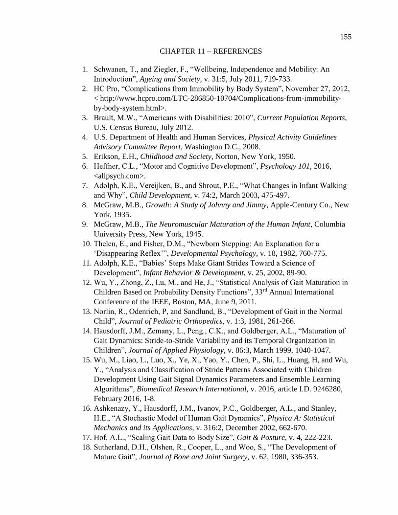
155
CHAPTER 11 – REFERENCES
1. Schwanen, T., and Ziegler, F., “Wellbeing, Independence and Mobility: An
Introduction”, Ageing and Society, v. 31:5, July 2011, 719-733.
2. HC Pro, “Complications from Immobility by Body System”, November 27, 2012,
< http://www.hcpro.com/LTC-286850-10704/Complications-from-immobility-
by-body-system.html>.
3. Brault, M.W., “Americans with Disabilities: 2010”, Current Population Reports,
U.S. Census Bureau, July 2012.
4. U.S. Department of Health and Human Services, Physical Activity Guidelines
Advisory Committee Report, Washington D.C., 2008.
5. Erikson, E.H., Childhood and Society, Norton, New York, 1950.
6. Heffner, C.L., “Motor and Cognitive Development”, Psychology 101, 2016,
<allpsych.com>.
7. Adolph, K.E., Vereijken, B., and Shrout, P.E., “What Changes in Infant Walking
and Why”, Child Development, v. 74:2, March 2003, 475-497.
8. McGraw, M.B., Growth: A Study of Johnny and Jimmy, Apple-Century Co., New
York, 1935.
9. McGraw, M.B., The Neuromuscular Maturation of the Human Infant, Columbia
University Press, New York, 1945.
10. Thelen, E., and Fisher, D.M., “Newborn Stepping: An Explanation for a
‘Disappearing Reflex’”, Developmental Psychology, v. 18, 1982, 760-775.
11. Adolph, K.E., “Babies’ Steps Make Giant Strides Toward a Science of
Development”, Infant Behavior & Development, v. 25, 2002, 89-90.
12. Wu, Y., Zhong, Z., Lu, M., and He, J., “Statistical Analysis of Gait Maturation in
Children Based on Probability Density Functions”, 33rd Annual International
Conference of the IEEE, Boston, MA, June 9, 2011.
13. Norlin, R., Odenrich, P, and Sandlund, B., “Development of Gait in the Normal
Child”, Journal of Pediatric Orthopedics, v. 1:3, 1981, 261-266.
14. Hausdorff, J.M., Zemany, L., Peng., C.K., and Goldberger, A.L., “Maturation of
Gait Dynamics: Stride-to-Stride Variability and its Temporal Organization in
Children”, Journal of Applied Physiology, v. 86:3, March 1999, 1040-1047.
15. Wu, M., Liao, L., Luo, X., Ye, X., Yao, Y., Chen, P., Shi, L., Huang, H, and Wu,
Y., “Analysis and Classification of Stride Patterns Associated with Children
Development Using Gait Signal Dynamics Parameters and Ensemble Learning
Algorithms”, Biomedical Research International, v. 2016, article I.D. 9246280,
February 2016, 1-8.
16. Ashkenazy, Y., Hausdorff, J.M., Ivanov, P.C., Goldberger, A.L., and Stanley,
H.E., “A Stochastic Model of Human Gait Dynamics”, Physica A: Statistical
Mechanics and its Applications, v. 316:2, December 2002, 662-670.
17. Hof, A.L., “Scaling Gait Data to Body Size”, Gait & Posture, v. 4, 222-223.
18. Sutherland, D.H., Olshen, R., Cooper, L., and Woo, S., “The Development of
Mature Gait”, Journal of Bone and Joint Surgery, v. 62, 1980, 336-353.

156
19. Ganley, K.J., and Powers, C.M., 2005, “Gait Kinematics and Kinetics of 7-Year-
Old Children: A Comparison to Adults Using Age-Specific Anthropometric
Data,” Gait & Posture, v. 21:2, 141-145.
20. Chester, V.L., Tingley, M., and Biden, E.N., 2006, “A Comparison of Kinetic
Gait Parameters for 3-13 Year Olds,” Clinical Biomechanics, v. 21:7, 726-732.
21. Chester, V.L., and Wrigley, A.T., 2008, “The Identification of Age-Related
Differences in Kinetic Gait Parameters Using Principal Component Analysis,”
Clinical Biomechanics, v. 23:2, 212-220.
22. Burnett, C.N., and Johnson, E.W., “Development of Gait in Childhood: Part II”,
Developmental Medicine & Child Neurology, v. 13:2, April 1971, 207-215.
23. Stansfield, B.W., Hillman, S.J., Hazlewood, M.E., Lawson, A.M., Mann, A.M.,
Loudon, I.R., and Robb, J.E., “Normalisation of Gait Data in Children”, Gait &
Posture, v. 17:1, 2003, 81-87.
24. Bernstein, N., The Coordination and Regulation of Movements, Pergamon Press,
Oxford, England, 1967.
25. Breniere, Y., and Bril, B., “Development of Postural Control of Gravity Forces in
Children During the First 5 Years of Walking”, Experimental Brain Research, v.
121, 1998, 255-262.
26. Bril, B., and Ledebt, A., “Head Coordination as a Means to Assist Sensory
Integration in Learning to Walk”, Neuroscience and Behavioral Reviews, v. 22,
1998, 555-563.
27. Keen, M., “Early Development and Attainment of Normal Mature Gait”, Journal
of Pediatric Orthopedics, v. 5:2, 1993, 35-38.
28. Dusing, S.C., and Thorpe, D.E., “A Normative Sample of Temporal and Spatial
Gait Parameters in Children Using the GAITRite Electronic Walkway”, Gait &
Posture, v. 25:1, 2007, 135-139.
29. Stansfield, B.W., Hillman, S.J., Hazlewood, M.E., and Robb, J.E., “Regression
Analysis of Gait Parameters with Speed in Normal Children Walking at Self-
Selected Speeds”, Gait & Posture, v. 23:3, 2006, 288-294.
30. Murphy, K.P., Matthews, D.J., and Alexander, M.A., Pediatric Rehabilitation:
Principles and Practice, Ed. 5, New York: Demos Medical, 2015.
31. Perry, J., Gait Analysis: Normal and Pathological Function, Thorofare, NJ: Slack
Inc, 1992.
32. Buzzi, U.H., Stergiou, N., Kurz, M.J., Hageman, P.A., and Heidel, J., “Nonlinear
Dynamics Indicates Aging Affects Variability During Gait”, Clinical
Biomechanics, v. 18:5, 2003, 435-443.
33. Hausdorff, J.M., Peng, C.K., Ladin, Z., Wei, J.Y., and Goldberger, A.L., “Is
Walking a Random Walk? Evidence for Long-Range Correlations in Stride
Interval of Human Gait”, Journal of Applied Physiology, v. 78:1, January 1995,
349-358.
34. Hausdorff, J.M., Mitchell, S.L., Firtion, R., Peng, C.K., Cudkowicz, M.E., Wei,
J.Y., and Goldberger, A.L., “Altered Fractal Dynamics of Gait: Reduced Stride-

157
Interval Correlations with Aging and Huntington’s Disease”, Journal of Applied
Physiology, v. 82:1, January 1997, 262-269.
35. Baker, G.L., and Gollub, J.P., Chaotic Dynamics, Cambridge University Press,
New York, 1996.
36. Abarbanel, H.D.I., Analysis of Observed Chaotic Data, Springer, New York,
1996.
37. Kurz, M.J., Chaos in Gait, Dissertation presented to the Graduate College at the
University of Nebraska, Omaha, Nebraska, 2006.
38. Johnson, E.O., and Soucacos, P.N., “Proprioception”, International Encyclopedia
of Rehabilitation, Center for International Rehabilitation Research Information
and Exchange, 2016. < http://cirrie.buffalo.edu/encyclopedia/en/article/337/>.
39. Aman, J.E., Elangovan, N., Yeh, I.L., and Konczak, J., “The Effectiveness of
Proprioceptive Training for Improving Motor Function: A Systematic Review”,
Frontiers in Human Neuroscience, v. 8, Article 1075, January 2015, 1-18.
40. Miller, J., “Proprioception & Balance Exercises”, Physioworks, Accessed October
14, 2016, < http://physioworks.com.au/treatments-1/proprioception-balance-
exercises>.
41. Carr, J.H., and Shepherd, R.B., A Motor Relearning Programme for Stroke, 2nd
Ed., Aspen Publishers, Rockville, MD, 1987.
42. Riskowski, J.L., Mikesky, A.E., Bahamonde, R.E., Alvey III, T.V., and Burr,
D.B., “Proprioception, Gait Kinematics, and Rate of Loading During Walking:
Are They Related?”, Journal of Musculoskeletal and Neuronal Interactions, v.
5:4, 2005, 379-387.
43. Kosak, M.C., and Reding, M.J., “Comparison of Partial Body Weight-Supported
Treadmill Gait Training Versus Aggressive Bracing Assisted Walking Post
Stroke”, Neurorehabilitation and Neural Repair, v. 14:1, March 2000, 13-19.
44. Wang, R.Y., “Effect of Proprioceptive Neuromuscular Facilitation on the Gait of
Patients with Hemiplegia of Long and Short Duration”, Physical Therapy, v.
74:12, December 1994, 1108-1115.
45. Zouita, A.B.M., Bousselmi, M., Darragi, M., Ferchichi, H., Dziri, C., and Ben
Salah, F.Z., “Proprioception Rehabilitation and Gait Parameters in Athletes after
Ankle Sprain”, Annals of Sports Medicine and Research, v. 3:5, 2016, 1077-1081.
46. LeMoyne, R., Coroian, C., Mastroianni, T., Opalinski, P., Cozza, M., and
Grundfest, W., “The Merits of Artificial Proprioception, With Applications in
Biofeedback Gait Rehabilitation Concepts and Movement Disorder
Characterization”, Biomedical Engineering, de Mello, C.A.B. (ed.), InTech,
Croatia, 2009, 165-198.
47. Lewek, M.D., Feasel, J., Wentz, E., Brooks Jr, F.P., and Whitton, M.C., “Use of
Visual and Proprioceptive Feedback to Improve Gait Speed and Spatiotemporal
Symmetry Following a Chronic Stroke: A Case Series”, Physical Therapy, v.
92:5, May 2012, 748-756.
48. Mirek, E., Chwala, W., Longawa, K., Rudzinska, M., Adamkiewicz, P., and
Szczudlik, A., “Proprioceptive Neuromuscular Facilitation Method of Therapeutic
158
Rehabilitation in the Treatment of Patients with Parkinson Disease”, Neurologia i
Neurochirurgia Polska, v. 37 Supplement 5, 2003, 89-102.
49. Kuo, A.D., and Donelan, J.M., “Dynamic Principles of Gait and their Clinical
Implications”, Physical Therapy, v. 90:2, February 2010, 157-176.
50. Eng, J.J., Tang, and Tang, P.F., “Gait Training Strategies to Optimize Walking
Ability in People with Stroke: A Synthesis of the Evidence”, Expert Review of
Neurotherapeutics, v. 7:10, 2007, 1417-1436.
51. Corbridge, L.M., Goldman, A.J., Shu, Y., Buster, T.W., and Burnfield, J.M.,
“Clinician’s Muscle Effort during Partial Body Weight Support Treadmill
Training: Is it Hard Work?”, Online Proceedings, American Physical Therapy
Association’s 2009 Annual Conference and Exposition, 2009,
<http://apps.apta.org/Custom/abstracts/pt2009/abstractsPt.cfm?m_id=19675>.
52. Visintin, M., Barbeau, H., Korner-Bitensky, N., and Mayo, N.E., “A New
Approach to Retrain Gait in Stroke Patients through Body Weight Support and
Treadmill Stimulation”, Stroke, v. 29, 1998, 1122-1128.
53. Kosak, M.C., and Reding, M.J., “Comparison of Partial Body Weight-Supported
Treadmill Gait Training Versus Aggressive Bracing Assisted Walking Post
Stroke”, Neurorehabilitation and Neural Repair, v. 14:1, March 2000, 13-19.
54. Damiano, D.L., Norman, T., Stanley, C.J., and Park, H.S., “Comparison of
Elliptical Training, Stationary Cycling, Treadmill Walking and Overground
Walking”, Gait & Posture, v. 34:2, June 2011, 260-264.
55. Banala, S.K., Kim, S.H., Agrawal, S.K., and Scholz, J.P., “Robot Asissted Gait
Training with Active Leg Exoskeleton (ALEX)”, IEEE Transactions on Neural
Systems and Rehabilitation Engineering, v. 17:1, February 2009, 2-8.
56. Olson, J., “Hospitals Have New Tool to Help Paralyzed Patients: Robotics”, Star
Tribune, May 31, 2016, <http://www.startribune.com/hospitals-have-new-tool-to-
help-paralyzed-patients-robotics/381213281/>.
57. Veneman, J.F., Kruidhof, R., Hekman, E.E.G., Ekklenkamp, R., Van Asseldonk,
E.H.F., and van der Kooij, H., “Design and Evaluation of the LOPES Exoskeleton
Robot for Interactive Gait Rehabilitation”, IEEE Transactions on Neural Systems
and Rehabilitation Engineering, v. 15:3, September 2007, 379-386.
58. Sale, P., Franceschini, M., Waldner, A., and Hesse, S., “Use of the Robot Assisted
Gait Therapy in Rehabilitation of Patients with Stroke and Spinal Cord Injury”,
European Journal of Physical and Rehabilitation Medicine, v. 48:1, 2012, 111-
121.
59. Peshkin, M., Brown, D.A., Santos-Munne, J.J., Makhlin, A., Lewis, E., Colgate,
J.E., Patton, J., and Schwandt, D., “KineAssist: A Robotic Overground Gait and
Balance Training Device”, 9th International Conference on Rehabilitation
Robotics, 2005.
60. Meyer-Heim, A., Ammann-Reiffer, C., Schmartz, A., Schafer, J., Sennhauser,
F.H., Heinen, F., Knecht, B., Dabrowski, E., and Borggraefe, I., “Improvement of
Walking Abilities after Robotic-Assisted Locomotion Training in Children with
Cerebral Palsy”, Archives of Disease in Childhood, v. 94, 2009, 615-620.

159
61. Hornby, G.T., Kinnaird, C.R., Holleran, C.L., Rafferty, M.R., Rodriguez, K.S.,
and Cain, J.B., “Kinematic, Muscular, and Metabolic Responses During
Exoskeletal-, Elliptical-, or Therapist-Assisted Stepping in People with
Incomplete Spinal Cord Injury”, Physical Therapy, v. 92:10, October 2012, 1278-
1291.
62. Hornby, T.G., Campbell, D.D., Kahn, J.H., Demott, T., Moore, J.L., and Roth,
H.R., “Enhanced Gait-Related Improvements after Therapist – Versus Robotic-
assisted Locomotor Training in Subjects with Chronic Stroke”, Stroke, v. 39,
2008, 1786-1792.
63. Ha, K.H., Murray, S.A., and Goldfarb, M., “An Approach for the Cooperative
Control of FES with a Powered Exoskeleton During Level Walking for Persons
with Paraplegia”, IEEE Transactions on Neural Systems and Rehabilitation
Engineering, v. 24:4, 2016, 455-466.
64. Farris, R.J., Quintero, H.A., and Goldfarb, M., “Preliminary Evaluation of a
Powered Lower Limb Orthosis to Aid Walking in Paraplegic Individuals”, IEEE
Transactions on Neural Systems and Rehabilitation Engineering, v. 19:6, 2011,
652-659.
65. Goldfarb, M., Lawson, B.E., and Shultz, A.H., “Realizing the Promise of Robotic
Leg Prostheses”, Science Translational Medicine, v. 5:210, 2013, 210.15.
66. Goldfarb, M., Farris, R.J., and Quintero, H.A., Movement Assistance Device, US
Patent Application No. 2014-049494, October 9, 2013.
67. Yeseta, M.C., Taylor, A.P., Buster, T.W., Shu, Y., and Burnfield, J.M., “Exercise
Endurance and Functional Mobility Improve for Individuals with Physical
Disabilities After Training on a Motorized Elliptical”, Rehabilitation Engineering
and Assistive Technology Conference, 2012.
68. Bradford, J.C., and Pidcoe, P.E., “Development of a Low-Cost Robotic Gait
Trainer”, Conference Proceedings of the Annual Meeting of the American Society
of Biomechanics, 2009, 1-2.
69. Tom-Wigfield, D., Haynes, E., and Martin, R., “Activity-Based Restorative
Therapy Steps into Robotic Gait Training for Innovative Approaches for Patients
with Chronic Spinal Cord Injuries”, Rehab Management, June 7, 2016.
70. Burnfield, J. M., Shu, Y., Buster. T. W., and Taylor. A., “Similarity of Joint
Kinematics and Muscle Demands between Elliptical Training and Walking:
Implications for Practice”, Physical Therapy, v. 90:2, 2010, 289-305.
71. Shyu, J. H., Chen, C. K., and Luo, Y. J., “Research and Development of an
Adjustable Elliptical Exerciser”, 13th World Congress in Mechanism and
Machine Science, Guanajuato, México, 19-25 June 2011.
72. Lin, M.P., Chang, Y.J., and Yu, M.D., “Phase-Dependent Modulation of Soleus
H-Reflex and Post-Activation Depression during Elliptical Trainer and Treadmill
Walking in Humans,” Physiotherapy, v. 101 Supplement 1, 3881.
73. Sawicki, G.S., Gordon, K.E., and Ferris, D.P., “Powered Lower Limb Orthoses:
Applications in Motor Adaptation and Rehabilitation”, Rehabilitation Robotics,
2005.
160
74. Meyer-Heim, A., Borggraefe, I., Ammann-Reiffer, C., Berweck, S., Sennhauser,
F. H., Colombo, G., Knecht, B. and Heinen, F., “Feasibility of Robotic-Assisted
Locomotor Training in Children with Central Gait Impairment”, Developmental
Medicine & Child Neurology, v. 49, 2007, 900-906.
75. Morrison, S., “Financial Feasibility of Robotics in Neurorehabilitation”, Spinal
Cord Injury Rehabilitation, v. 17:1, 2011, 77-81.
76. Mehrholz, J., Elsner, B., Werner, C., Kugler, J., and Pohl, M.,
“Electromechanical-Assisted Training for Walking After Stroke”, Cochrane
Database of Systematic Reviews, v. 7, 2013, Article CD006185, Wiley,
<http://onlinelibrary.wiley.com/doi/10.1002/14651858.CD006185.pub3/epdf>.
77. Dundar, U., Toktas, H., Solak, O., Ulasli, A.M., and Eroglu, S., “A Comparative
Study of Conventional Physiotherapy Versus Robotic Training Combined with
Physiotherapy in Patients with Stroke”, Topics in Stroke Rehabilitation, v. 21:6,
2014, 453-461.
78. Fasoli, S. E., Ladenheim, B., Mast, J., and Krebs, H. I., “New Horizons for Robot-
Assisted Therapy in Pediatrics”, American Journal of Physical Medicine &
Rehabilitation, v. 91:11, November 2012, S280–S289.
79. Langhorne, P., Coupar, F., and Pollock, A., “Motor Recovery After Stroke: A
Systematic Review”, The Lancet Neurology, v8:8, August 2009, 741-754.
80. Nelson, C.A., Burnfield, J.M., Shu, Y., Buster, T.W., Taylor, A.P., and Graham,
A., “Modified Elliptical Machine Motor-Drive Design for Assistive Gait
Rehabilitation,” Journal of Medical Devices, v. 5:2, 2011.
81. Burnfield, J.M., Shu, Y., Buster, T.W., Taylor, A., and Nelson, C.A., “Impact of
Elliptical Trainer Ergonomic Modifications on Perceptions of Safety, Comfort,
Workout and Usability by Individuals with Physical Disabilities and Chronic
Conditions”, Physical Therapy, v. 91:11, 2011, 1604-1617.
82. Burnfield, J.M., Irons, S.L., Buster, T.W., Taylor, A.P., Hildner, G.A., and Shu,
Y., “Comparative Analysis of Speed’s Impact on Muscle Demands During Partial
Body Weight Support Motor-Assisted Elliptical Training”, Gait and Posture, v.
39:1, 2014, 314-320.
83. Burnfield, J.M., Shu, Y., Buster, T.W., and Taylor, A.P., “Similarity of Joint
Kinematics and Muscle Demands Between Elliptical Training and Walking:
Implications for Practice”, Physical Therapy, v. 90:2, 2010, 289-305.
84. "Introduction", NRAS, July 18, 2016, <http://www.nras.org.uk/introduction>.
85. Pinney, S., Ed., “Bones and Joints of the Foot and Ankle Overview”, Foot
Education, October 17, 2015, <http://www.footeducation.com>.
86. Cronin, N.J., “The Effects of High Heeled Shoes on Female Gait: A Review”,
Journal of Electromyography and Kinesiology, v. 24:2, April 2014, 258-263.
87. Nadége, K.F.E, Jean-Marie, F., Mansourou, L.M., Polycarpe, G., Gabriel, A.Y.,
and Sophia, L., “Wearing High Heel Shoes During Gait: Kinematics Impact and
Determination of Comfort Height”, American Journal of Life Sciences, v. 3:2,
2015, 56-61.

161
88. Nwankwo, M.J., Egwuonwu, A.V., Ezeukwu, A.O., and Nwafulume, C.K.,
“Effects of Different Heel Heights on Selected Gait Parameters of Young
Undergraduate Females”, Journal of Paramedical Sciences, v. 3:3, 2012, 9-14.
89. Esenyel, M., Walsh, K., Walden, J.G., and Gitter, A., “Kinetics of High-Heeled
Gait”, Journal of the American Podiatric Medical Association, v. 93:1, January
2003, 27-32.
90. Barkema, D., The Effect of Heel Height on Frontal Plane Joint Moments, Impact
Acceleration, and Shock Attenuation During Walking, A Thesis, Iowa State
University, 2010.
91. Winter, D.A., “Foot Trajectory in Human Gait: A Precise and Multifactorial
Motor Control Task”, Phys Ther., Issue 72, January 1992, 45-53.
92. Fang, J., and Hunt, K.J., “Foot Trajectory Approximation Using the Pendulum
Model of Walking”, Medical and Biological Engineering and Computation, 52nd
ed., 2014, 45-52.
93. Fang, J., Hunt, K.J., Xie, L., and Yang, G.Y., “Modelling of the Toe Trajectory
During Normal Gait using Circle-Fit Approximation”, Medical and Biological
Engineering and Computation, v. 54, 2016, 1481-1489.
94. Burnfield, J.M., Taylor, A.P., Buster, T.W., Shu, Y., Goldman, A.J., and Nelson,
C.A., Use of Intelligently Controlled Assistive Rehabilitation Elliptical Trainer to
Improve Walking and Fitness during Acute Stroke Rehabilitation”, Stroke, v.
42:3, 2011, e326.
95. Buster, T.W., Burnfield, J.M., Taylor, A.P., and Stergiou, N., “Lower Extremity
Kinematics During Walking and Elliptical Training in Individuals With and
Without Traumatic Brain Injury”, Journal of Neurologic Physical Therapy, 37:4,
2013, 176-186.
96. Irons, S.L., Brusola, G.A., Buster, T.W., and Burnfield, J.M., “Novel ICARE
Intervention Improves Six-Minute Walk Test and Oxygen Cost for an Individual
with Progressive Supranuclear Palsy”, Cardiopulmonary Physical Therapy
Journal, v. 26:2, 2015, 36-41.
97. Irons, S.L., Burnfield, J.M., Buster, T.W., Karkowski-Schelar, E., and Johns, E.,
Individuals with Multiple Sclerosis Improved Walking Endurance and Decreased
Fatigue Following Motor-Assisted Elliptical Training Intervention”, Accepted,
2016 American Congress of Rehabilitation Medicine (ACRM), 93rd Annual
Conference: Progress in Rehabilitation Research. Chicago, IL, November 3, 2016.
98. Budynas, R.G., and Nisbett, K.J., Shigley’s Mechanical Engineering Design, 8th
ed., McGraw Hill, New York, 2008.
99. ASM International, “Fatigue”, Elements of Metallurgy and Engineering Alloys,
2008, 243-264.
100. Hallquist, J.O., LS-DYNA Keyword User’s Manual, Livermore Software
Technology Corporation, Livermore, CA, 2001.
101. Burnfield, J.M., Buster, T.W., Irons, S.L., Cesar, G.M., Nelson, C.A., Rech,
N.R., and Nichols, E.M., “Pediatric Walking vs. Training on Prototype Motor-
Assisted Elliptical: Kinematic comparison at self-selected comfortable speed.

162
Accepted, 2016 American Congress of Rehabilitation Medicine (ACRM) 93rd
Annual Conference: Progress in Rehabilitation Research, Chicago, IL,
November 3, 2016.
102. Burnfield, J.M., Buster, T.W., Irons, S.L., Rech, N., Cesar, G.M., Pfeifer, C.M.,
and Nelson, C.A., “Pediatric Intelligently Controlled Assistive Rehabilitation
Elliptical for Walking and Fitness: Prototype Development and Biomedical
Analysis”, Presented at RESNA/NCART (Rehabilitation Engineering Society of
North America/National Coalition for Assistive and Rehab Technology) 2016
annual convention, July 10-14, Arlington, VA.
103. Buster, T.W., Burnfield, J.M., Irons, S.L., Nelson, C.A., Trejo, L.H., and
Leutzinger, T.J., “Pediatric Walking vs. Training on a Prototype Motor-Assisted
Elliptical: Kinematic and EMG Comparisons at Self-Selected Fast Speeds”,
Conference proceedings, 2016 Annual Meeting Gait and Clinical Movement
Analysis Society, Memphis, TN, May 17-20, 2016.
104. Zhang, Y., Finger, S., and Behrens, S., “Planar Linkages”, Introduction to
Mechanisms, Carnegie Mellon University, Pittsburgh, PA, 2010,
<https://www.cs.cmu.edu/~rapidproto/mechanisms/chpt5.html>.
105. “Kinematic Inversions of Four Bar Chain, Slider Crank and Double Slider
Crank Mechanism”, Engineering Tutorials, March 14, 2013,
<http://engineering.myindialist.com/2013/kinematic-inversions-of-four-bar-
chain-slider-crank-and-double-slider-crank-mechanism/#.WAsGc-ArK00>.
106. Hrones, J.A., and Nelson, G.L., Analysis of the Four-Bar Linkage, Massachusetts
Institute of Technology, New York, 1951.
107. Freudenstein, F., “An Analytical Approach to the Design of Four-Link
Mechanisms”, American Society of Mechanical Engineers, v. 76:3, April 1954,
483–492.
108. Murray ,A.P., and McCarthy, J.M., “Determining Burmester Points from the
Analysis of a Planar Platform”, Journal of Mechanical Design, v. 117, June
1995, 303-307.
109. Kunjur, A., and Krishnamurty, S., "Genetic Algorithms in Mechanism
Synthesis." University of Massachussetts, Accessed May 4, 2014,
<http://www.ecs.umass.edu/mie/labs/mda/mechanism/papers/genetic.html>.
110. Roston, G.P., and Sturges, R.H., "Genetic Algorithm Synthesis of Four-Bar
Mechanisms", Pennsylvania State University, Accessed May 4, 2014,
<http://citeseerx.ist.psu.edu/viewdoc/download?doi=10.1.1.119.9140&rep=rep1
&type=pdf>.
111. Dulger, L.C., Erdogan, H., and Kutuk, M.E., “Matlab’s GA and Optimization
Toolbox: A Fourbar Mechanism Application”, International Journal of
Intelligent Systems and Application in Engineering, Vol. 2, Ed. 1, 10-15.
112. Li, J,. “The Optimization Design of the Four-Bar Linkage Based on MATLAB”,
International Conference on Intelligent Systems Research and Mechatronics
Engineering, 2015, 788-791.

163
113. Vilas, C.P., and Ghosal, A., “Optimal Synthesis of Adjustable Planar Four-Bar
Crank-Rocker Type Mechanisms for Approximate Multi-Path Generation”,
Indian Institute of Science Department of Mechanical Engineering, Accessed
October 22, 2016, 1-29, <http://www.mecheng.iisc.ernet.in/~asitava/chanekar-
1.pdf>.
114. Lanni, C., and Ceccarelli, M., “An Optimization Problem Algorithm for
Kinematic Design of Mechanisms for Two-Finger Grippers”, The Open
Mechanical Engineering Journal, v. 3, 2009, 49-62.
115. “How to Make a Pantograph”, 1920-20.com, 2012, <http://www.1920-
30.com/toys/things-to-make/pantograph.html>.
116. Goldstein, R., and Veloso, M., “Extendable Pantograph Arms”, Association for
the Advancement of Artificial Intelligence, 2016,
<https://www.aaai.org/ocs/index.php/SSS/SSS16/paper/download/12727/11931>
.
117. Long, H., Yang, Y., Jingjing, X., and Peng, S., “Type Synthesis of 1R1T Remote
Center of Motion Mechanisms Based on Pantograph Mechanisms”, Journal of
Mechanical Design, v. 138, January 2016, 014501-1-5.
118. Rojas, R., “Genetic Algorithms”, Neural Networks, Springer-Verlag, Berlin,
1996, 429-450.
119. Bertsekas, D.P., Constrained Optimization and Lagrange Multiplier Methods,
Massachusetts Institute of Technology, 1996.
120. “Gradient Projection Methods”, NEOS Optimization Guide, University of
Wisconsin-Madison, <http://www.neos-guide.org/content/gradient-projection-
methods>.
121. Dolan, E., The NEOS Server 4.0 Administrative Guide, Technical Memorandum
ANL/MCS-TM-250, Mathematics and Computer Science Division, Argonne
National Laboratory, 2001.
122. Zhang, Y., Finger, S., and Behrens, S., “Cams”, Introduction to Mechanisms,
Carnegie Mellon University, Pittsburgh, PA, 2010,
123. Johns, W.E., “Notes on Sprockets and Chains”, Gizmology.net, 2003,
<http://www.gizmology.net/sprockets.htm>.
124. Ryabov, G.K., and Serzhantova, L.P., Minimum Possible Contact Angle of
Chain Transmission Sprockets, January 1985.
125. Nelson, C.A., Stolle, C.J., Burnfield, J.M., Buster, T.W., and McCrory, B.J.,
Assistive Rehabilitation Elliptical System, US Patent Application No. US 2016-
023788, September 29, 2016.
126. Nelson, C.A., Stolle, C.J., Burnfield, J.M., and Buster, T.W., “Modification of
the ICARE System for Pediatric Therapy”, Journal of Medical Devices, V. 9 (4),
Published online August 6, 2015.
127. Nelson, C.A., Stolle, C.J., Burnfield, J.M., and Buster, T.W., “Synthesis of a
Rehabilitation Mechanism Replicating Normal Gait”, 14th IFToMM World
Congress Proceedings, OS1-016, October 25, 2015.

164
128. Stolle, C.J., Nelson, C.A., Burnfield, J.M., and Buster, T.W., “Improved Design
of a Gait Rehabilitation Robot”, Proceedings of the 5th International Workshop
on Medical and Service Robots, Graz, Austria, July 4-6, 2016.

165
APPENDIX A – FOURIER SERIES MODELING OF FOOT GAIT PATHS
Pediatric Metatarsal Data
Pediatric Cartesian Metatarsal Parametrization Comparison (ox=2,oy=6)
Pediatric Cartesian Metatarsal Trajectory Comparison (ox=2,oy=6)

166
Pediatric Cartesian Metatarsal Trajectory Comparison (ox=8,oy=8)
Fourier Series Terms for Pediatric Metatarsal Trajectory
m,n a b a b
0 0.00390 0.01885
1 -0.00149 0.44097 0.90534 -0.02920 -0.00245 0.61266
2 0.00345 -0.13606 0.99158 0.01023 0.00021 0.68802
3 -0.00359 0.04140 0.99963 0.00597 0.00571 0.73625
4 0.00255 -0.00695 0.99988 -0.01120 -0.00981 0.89382
5 -0.00104 -0.00201 0.99990 0.00750 0.00845 0.98476
6 0.00094 0.00363 0.99997 -0.00211 -0.00345 0.99644
7 -0.00053 -0.00120 0.99998 -0.00040 -0.00069 0.99690
8 0.00069 -0.00027 0.99998 0.00041 0.00173 0.99914
X-Coordinate Y-Coordinate
Pediatric Am and Bn Constants
R^2 R^2
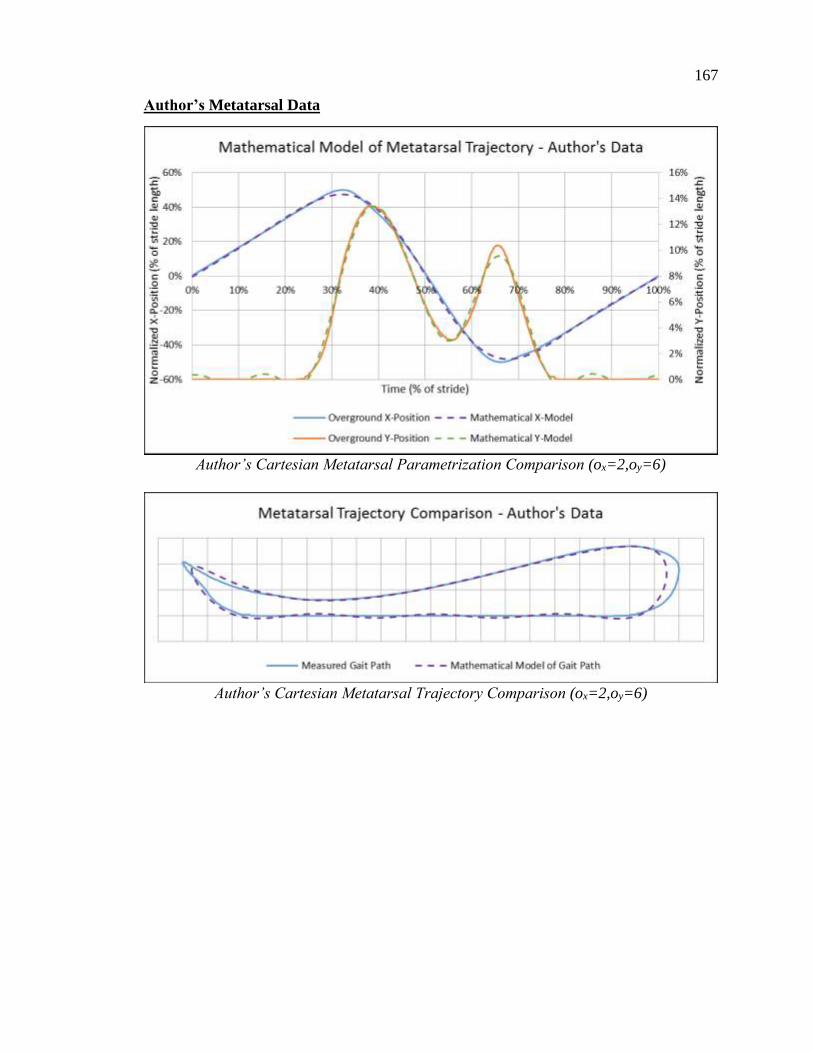
167
Author’s Metatarsal Data
Author’s Cartesian Metatarsal Parametrization Comparison (ox=2,oy=6)
Author’s Cartesian Metatarsal Trajectory Comparison (ox=2,oy=6)
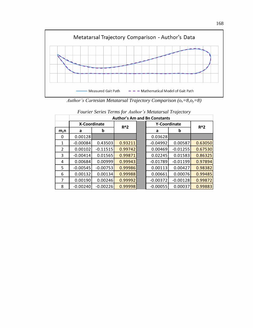
168
Author’s Cartesian Metatarsal Trajectory Comparison (ox=8,oy=8)
Fourier Series Terms for Author’s Metatarsal Trajectory
m,n a b a b
0 0.00128 0.03628
1 -0.00084 0.43503 0.93211 -0.04992 0.00587 0.63050
2 0.00102 -0.11515 0.99742 0.00469 -0.01255 0.67530
3 -0.00414 0.01565 0.99871 0.02245 0.01583 0.86325
4 0.00684 0.00999 0.99943 -0.01789 -0.01199 0.97894
5 -0.00545 -0.00753 0.99986 0.00113 0.00427 0.98382
6 0.00132 0.00134 0.99988 0.00661 0.00076 0.99485
7 0.00190 0.00246 0.99992 -0.00372 -0.00128 0.99872
8 -0.00240 -0.00226 0.99998 -0.00055 0.00037 0.99883
X-Coordinate Y-Coordinate
Author's Am and Bn Constants
R^2 R^2

169
Winter’s Metatarsal Data
Winter’s Cartesian Metatarsal Parametrization Comparison (ox=2,oy=6)
Winter’s Cartesian Metatarsal Trajectory Comparison (ox=2,oy=6)

170
Winter’s Cartesian Metatarsal Trajectory Comparison (ox=8,oy=8)
Fourier Series Terms for Winter’s Metatarsal Trajectory
m,n a b a b
0 0.00055 0.03505
1 -0.00711 0.44439 0.95824 -0.04216 0.00115 0.58105
2 0.00426 -0.09081 0.99836 -0.00722 -0.01001 0.62845
3 -0.00304 0.00772 0.99870 0.02340 0.01643 0.89298
4 0.00425 0.01054 0.99932 -0.01039 -0.01303 0.98326
5 0.00080 -0.00195 0.99935 -0.00266 0.00141 0.98595
6 -0.00015 0.00074 0.99936 0.00366 0.00317 0.99409
7 0.00044 0.00292 0.99940 0.00057 -0.00081 0.99442
8 -0.00233 0.00074 0.99940 -0.00171 -0.00003 0.99524
X-Coordinate Y-Coordinate
Winter's Am and Bn Constants
R^2 R^2

171
Average Metatarsal Data
Average Winter’s Cartesian Metatarsal Parametrization Comparison (ox=8,oy=8)
Average Cartesian Metatarsal Trajectory Comparison (ox=8,oy=8)

172
Fourier Series Terms for Average Metatarsal Trajectory
m,n a b a b
0 0.001952 0.030684
1 -0.00321 0.449314 -0.04127 0.001555
2 0.002967 -0.11639 0.00262 -0.0076
3 -0.00367 0.022039 0.017633 0.01292
4 0.004643 0.004623 -0.01344 -0.01185
5 -0.00193 -0.00391 0.002033 0.004808
6 0.000715 0.001944 0.002778 0.000164
7 0.000618 0.001426 -0.00121 -0.00095
8 -0.00138 -0.00061 -0.00063 0.000702
Average Metatarsal Am and Bn Constants
X-Coordinate Y-Coordinate

173
Pediatric Heel Data
Pediatric Cartesian Heel Parametrization Comparison (ox=2,oy=3)
Pediatric Cartesian Heel Trajectory Comparison (ox=2,oy=3)

174
Pediatric Cartesian Heel Trajectory Comparison (ox=8,oy=8)
Fourier Series Terms for Pediatric Heel Trajectory
m,n a b a b
0 0.03199 0.08048
1 -0.05539 0.44963 0.93842 -0.12603 0.05731 0.66035
2 0.04444 -0.10243 0.99543 0.06275 -0.06301 0.93283
3 -0.02571 0.00799 0.99877 -0.01672 0.03768 0.99133
4 0.01083 0.01075 0.99983 -0.00109 -0.01481 0.99891
5 -0.00097 -0.00432 0.99992 0.00314 0.00372 0.99972
6 -0.00104 0.00059 0.99993 -0.00049 -0.00065 0.99975
7 0.00167 0.00230 0.99996 -0.00076 -0.00069 0.99978
8 -0.00012 -0.00061 0.99929 0.00074 0.00165 0.99990
X-Coordinate Y-Coordinate
Pediatric Heel Am and Bn Constants
R^2 R^2

175
Author’s Heel Data
Author’s Cartesian Heel Parametrization Comparison (ox=2,oy=3)
Author’s Cartesian Heel Trajectory Comparison (ox=2,oy=3)

176
Author’s Cartesian Heel Trajectory Comparison (ox=8,oy=8)
Fourier Series Terms for Author’s Heel Trajectory
m,n a b a b
0 0.04155 0.08345
1 -0.07263 0.42644 0.95394 -0.13008 0.05684 0.69004
2 0.04821 -0.07173 0.99203 0.05770 -0.06485 0.94807
3 -0.01952 -0.02139 0.99630 -0.00929 0.03592 0.99518
4 0.00062 0.02492 0.99947 -0.00341 -0.00831 0.99794
5 0.00446 -0.00457 0.99968 0.00138 -0.00376 0.99849
6 -0.00159 -0.00556 0.99985 0.00104 0.00534 0.99950
7 -0.00139 0.00425 0.99995 -0.00125 -0.00235 0.99975
8 0.00096 0.00045 0.99996 0.00061 -0.00081 0.99978
X-Coordinate Y-Coordinate
Author's Heel Am and Bn Constants
R^2 R^2

177
Winter’s Heel Data
Winter’s Cartesian Heel Parametrization Comparison (ox=2,oy=3)
Winter’s Cartesian Heel Trajectory Comparison (ox=2,oy=3)

178
Winter’s Cartesian Heel Trajectory Comparison (ox=8,oy=8)
Fourier Series Terms for Winter’s Heel Trajectory
m,n a b a b
0 0.04585 0.08267
1 -0.09804 0.43456 0.97056 -0.11803 0.07442 0.76376
2 0.05621 -0.03823 0.99338 0.04113 -0.06036 0.97265
3 -0.01561 -0.02489 0.99760 -0.00529 0.02355 0.99539
4 0.00001 0.01581 0.99883 0.00030 -0.00487 0.99629
5 0.00261 0.00827 0.99916 -0.00209 -0.00223 0.99671
6 0.00047 -0.00379 0.99920 0.00229 0.00312 0.99738
7 0.00108 0.00113 0.99921 -0.00074 0.00145 0.99749
8 -0.00248 0.00424 0.99927 -0.00063 -0.00302 0.99786
X-Coordinate Y-Coordinate
Winter's Heel Am and Bn Constants
R^2 R^2

179
Average Heel Data
Average Cartesian Heel Parametrization Comparison (ox=8,oy=8)
Average Cartesian Heel Trajectory Comparison (ox=8,oy=8)

180
Fourier Series Terms for Average Heel Trajectory
m,n a b a b
0 0.040722 0.084108
1 -0.0771 0.447013 -0.12761 0.064313
2 0.050769 -0.07244 0.055108 -0.06419
3 -0.02075 -0.01306 -0.01068 0.033135
4 0.003907 0.017561 -0.00143 -0.00955
5 0.002082 -0.00021 0.000826 -0.00077
6 -0.00074 -0.00299 0.000967 0.002664
7 0.000463 0.00262 -0.00094 -0.00054
8 -0.00056 0.00139 0.000245 -0.00074
Average Heel Am and Bn Constants
X-Coordinate Y-Coordinate

181
Pediatric Foot Angle Data
Pediatric Foot Angle Comparison (ox=3)
Pediatric Foot Angle Comparison (ox=8)

182
Fourier Series Terms for Pediatric Foot Angle
m,n a b
0 8.545291
1 -11.2107 12.39033 0.59644
2 2.078406 -12.3024 0.92820
3 1.381781 5.348146 0.99319
4 -0.82889 -0.16663 0.99472
5 -0.12025 -1.25694 0.99812
6 0.232149 0.552856 0.99889
7 -0.16688 0.205267 0.99903
8 0.179615 -0.48264 0.99960
X-CoordinateR^2
Pediatric Am and Bn Constants

183
Author’s Foot Angle Data
Author’s Foot Angle Comparison (ox=5)
Author’s Foot Angle Comparison (ox=8)

184
Fourier Series Terms for Author’s Foot Angle
m,n a b
0 13.13296
1 -17.4539 24.31764 0.58540
2 3.485944 -23.3338 0.94892
3 0.975032 6.980353 0.98136
4 0.351219 3.360969 0.98881
5 -0.54635 -3.57697 0.99736
6 -0.05078 0.392631 0.99747
7 0.236929 1.383102 0.99875
8 -0.29699 -1.1244 0.99964
Foot AngleR^2
Author's Am and Bn Constants
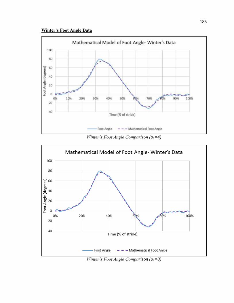
185
Winter’s Foot Angle Data
Winter’s Foot Angle Comparison (ox=4)
Winter’s Foot Angle Comparison (ox=8)

186
Fourier Series Terms for Winter’s Foot Angle
m,n a b
0 13.73055
1 -15.8727 32.37969 0.71515
2 0.936005 -21.9507 0.97963
3 1.223366 2.272873 0.98331
4 -0.99845 4.46098 0.99486
5 0.542386 -1.58599 0.99651
6 0.469622 -1.12671 0.99721
7 -0.28759 0.792762 0.99759
8 -0.21619 0.214468 0.99761
Foot AngleR^2
Winter's Am and Bn Constants

187
Average Foot Angle Data
Average Foot Angle Comparison (ox=8)
Fourier Series Terms for Average Foot Angle
m,n a b
0 11.80293
1 -14.8457 23.02922
2 2.166785 -19.1956
3 1.193393 4.867124
4 -0.49204 2.551773
5 -0.0414 -2.13996
6 0.216997 -0.06041
7 -0.07251 0.79371
8 -0.11119 -0.46419
X-Coordinate
Average Foot Angle Am and Bn
Constants

188
APPENDIX B – PART DIAGRAMS OF PEDIATRIC ICARE CRANK
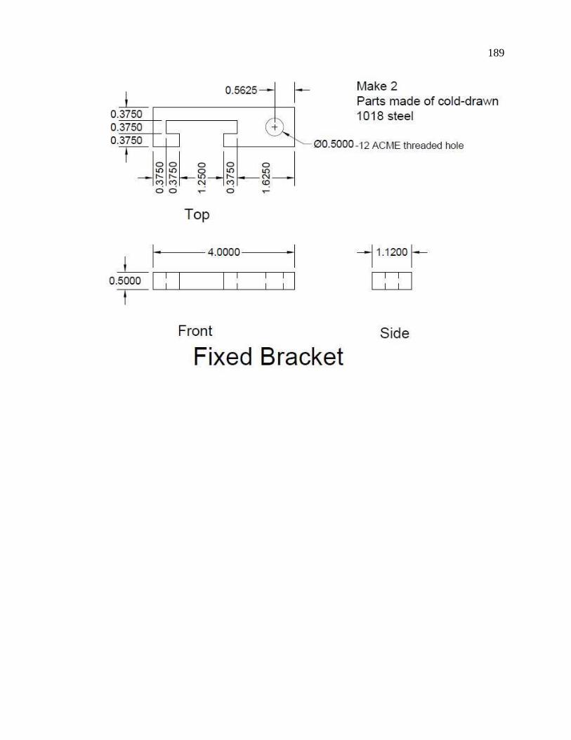
189

190

191

192

193
APPENDIX C NONLINEAR OPTIMIZATION OF ROCKER ANGULAR POSITION
USING MATLAB
% The period is normalized to 1 second. % The data begins with the foot positioned at centerline of stride.
%%%%%%%%%%%%%%%%%%%%%%%%%%%%%%%%%%%%%%%%%%%%%%%%%%%%%%%%%%%%%%%%%%%%%%%
%%%% %%%%%%%%%%%%%%%%%%%%%%%%%%%%%%%%%%%%%%%%%%%%%%%%%%%%%%%%%%%%%%%%%%%%%%%
%%%% % Set time and constant values for Fourier series
% Fourier Am and Bn constants Am = [-0.016352666; -0.374850467; -0.114519546; -0.001371391; -
0.006903369; -0.006738177; -0.000660878; -0.003511986; -0.002300941]; Bn = [-0.239342072; 0.057472015; 0.026786152; -0.002042114;
0.004048092; 0.002331935; -0.000816269; 0.001939239];
%Number of data points N = 201;
% Set time values t = zeros(N,1); for j = 1:N t(j,1) = (j-1)/(N-1); end
% Fourier-Determined Angular Curve FourierM = [Am(1)*ones(N,1) + Am(2)*cos(2*pi*t) + Bn(1)*sin(2*pi*t) +
Am(3)*cos(2*pi*2*t) + Bn(2)*sin(2*pi*2*t) + Am(4)*cos(3*pi*2*t) +
Bn(3)*sin(3*pi*2*t) + Am(5)*cos(4*pi*2*t) + Bn(4)*sin(4*pi*2*t) +
Am(6)*cos(5*pi*2*t) + Bn(5)*sin(5*pi*2*t) + Am(7)*cos(6*pi*2*t) +
Bn(6)*sin(6*pi*2*t) + Am(8)*cos(7*pi*2*t) + Bn(7)*sin(7*pi*2*t) +
Am(9)*cos(8*pi*2*t) + Bn(8)*sin(8*pi*2*t)]; FourierM = FourierM + ones(N,1)*0.5; %Adjusts the lowest Fourier series
point to 0
%%%%%%%%%%%%%%%%%%%%%%%%%%%%%%%%%%%%%%%%%%%%%%%%%%%%%%%%%%%%%%%%%%%%%%%
%%%% %%%%%%%%%%%%%%%%%%%%%%%%%%%%%%%%%%%%%%%%%%%%%%%%%%%%%%%%%%%%%%%%%%%%%%%
%%%% % Set initial values for independent parameters
% Link Lengths L1 = 8.0; L2 = 14.0; L3 = 16.0; L4 = 19.6977;
%Set Theta value theta = zeros(N,1); for m = 1:N; theta(m) = (m-1)/(N-1)*2*pi;

194
end
% Set constants for the Wolfe Conditions C = 0.0001;
%Define vector dimensions f = 0; fnew = 0; xnew = zeros(4,1);
A3 = zeros(N,1); dA3dx4 = zeros(N,1); dA3dx1 = zeros(N,1);
Psi = zeros(N,1); dPsidx1 = zeros(N,1); dPsidx4 = zeros(N,1);
phi = zeros(N,1); normphi = zeros(N,1); newphi = zeros(N,1); Jacobian =
zeros(N,4);
alpha0 = pi; % Initial value of alpha rho = 0.6; % Constant that alpha is multiplied by to test function
decrease k = 0; % Number of iterations done = 0; % Parameter that ends the program
x = [ L1; L2; L3; L4]; %%%%%%%%%%%%%%%%%%%%%%%%%%%%%%%%%%%%%%%%%%%%%%%%%%%%%%%%%%%%%%%%%%%%%%%
%%%% %%%%%%%%%%%%%%%%%%%%%%%%%%%%%%%%%%%%%%%%%%%%%%%%%%%%%%%%%%%%%%%%%%%%%%%
%%%% while done == 0 %%% Determine the constants R1, R2, and R3 R1 = x(4) / x(3); R2 = x(4) / x(1); R3 = (x(1)^2 + x(3)^2 + x(4)^2 - x(2)^2) / (2 * x(1) * x(3));
dR3dx1 = 1/(2*x(3)) + (x(3)^2 + x(4)^2 - x(2)^2)/(2*x(1) * x(3)); dR3dx2 = -1 * x(2) / (x(1) * x(3)); dR3dx3 = 1/(2*x(1)) + (x(1)^2 + x(4)^2 - x(2)^2)/(2*x(1) * x(3)); dR3dx4 = x(4) / (x(1) * x(3));
for m=1:N
%%%Calculate derivatives and function values
%A3 A3(m) = ((cos(theta(m)) + R2)^2 + sin(theta(m))^2)^(1/2); dA3dx4(m) = 2 * (cos(theta(m)) + R2) / (x(1) * ((cos(theta(m))
+ R2)^2 + sin(theta(m))^2)^(1/2)); dA3dx1(m) = -2 * x(4) * (cos(theta(m)) + R2) / (x(1)^2 *
((cos(theta(m)) + R2)^2 + sin(theta(m))^2)^(1/2));
%Psi Psi(m) = atan(-1 * sin(theta(m)) / (cos(theta(m)) + R2)); dPsidx4(m) = 1 / (x(1) * (1 - (sin(theta(m)) / (cos(theta(m)) +
R2))^2));

195
dPsidx1(m) = -x(4) / (x(1)^2 * (1 - (sin(theta(m)) /
(cos(theta(m)) + R2))^2));
%Phi phi(m) = acos((R1 * cos(theta(m)) + R3) / A3(m)) - Psi(m); if cos(phi(m)-theta(m)) + R2 * cos(phi(m)) - (R1 *
cos(theta(m)) + R3) > 1*10^-8 phi(m) = phi(m); else phi(m) = -phi(m); end
% Calculate the Jacobian for determining steepest descent Jacobian(m,1) = -1 / (1-((R1 * cos(theta(m)) + R3) /
A3(m))^2)^(-1/2) * (dR3dx1 / A3(m) -
(R1*cos(theta(m))+R3)/(A3(m)^2)*dA3dx1(m)) - dPsidx1(m); Jacobian(m,2) = -1 / (1-((R1 * cos(theta(m)) + R3) /
A3(m))^2)^(-1/2) * (dR3dx2 / A3(m)); Jacobian(m,3) = -1 / (1-((R1 * cos(theta(m)) + R3) /
A3(m))^2)^(-1/2) * (dR3dx3 / A3(m) - x(4)/x(3)^2 *
cos(theta(m))/A3(m)); Jacobian(m,4) = -1 / (1-((R1 * cos(theta(m)) + R3) /
A3(m))^2)^(-1/2) * (dR3dx4 / A3(m) - x(4)/x(3)^2 * cos(theta(m))/A3(m)
- (R1*cos(theta(m))+R3)/(A3(m)^2)*dA3dx4(m)) - dPsidx4(m); end
%The rocker angle in the comparison data starts at the minimum
value at %t = 0 seconds. In order to compare these two functions, we have to %change the projected rocker angle to match this. f = 0;
[offsetAng,I] = min(phi); for m = 1:N; if m+I > N normphi(m) = phi(m+I-N)-offsetAng; else normphi(m) = phi(m+I)-offsetAng; end
% Define function values f = f + (normphi(m) - FourierM(m))^2; end
NormValues = normphi; %For plotting purposes
%The gradient is the Jacobian multiplied by the function values. grad = transpose(Jacobian) * (normphi - FourierM);
%Define the descent vector p p = -0.1 * grad; %For Steepest Descent
xnew = x+p; if xnew(1) < 6 xnew = xnew * 6/xnew(1);

196
end
%Impose Grashof Conditions Grashof = 0; while Grashof == 0 if xnew(2) + xnew(4) > xnew(1) + xnew(3) if xnew(3) + xnew(4) > xnew(1) + xnew(2) if xnew(2) + xnew(3) > xnew(1) + xnew(4) Grashof = 1; else p = p * 1.1; p(1) = p(1)/1.1; end else p = p * 1.1; p(1) = p(1)/1.1; end else p = p * 1.1; p(1) = p(1)/1.1; end xnew = x + p; end
ready = 0; alpha = alpha0;
while ready == 0 %R values R1 = xnew(4) / xnew(3); R2 = xnew(4) / xnew(1); R3 = (xnew(1)^2 + xnew(3)^2 + xnew(4)^2 - xnew(2)^2) / (2 *
xnew(1) * xnew(3));
for m=1:N;
A3(m) = ((cos(theta(m)) + R2)^2 + sin(theta(m))^2)^(1/2);
Psi(m) = atan(-1 * sin(theta(m)) / (cos(theta(m)) + R2));
newphi(m) = acos((R1 * cos(theta(m)) + R3) / A3(m)) - Psi(m);
end if imag(newphi)==0 fnew = 0; phi = newphi; [offsetAng,I] = min(phi); for m = 1:N; if m+I > N normphi(m) = phi(m+I-N)-offsetAng; else normphi(m) = phi(m+I)-offsetAng;
% Define function values

197
fnew = fnew + (normphi(m) - FourierM(2))^2; end end
%Test to see if new r value meets the Wolfe criteria %%%if fnew > f + C * alpha *transpose(grad) * p; if fnew > f alpha = rho * alpha; xnew = x + alpha * p; else ready = 1; display(fnew) end else xnew = x; end if alpha < 1 * 10^8 p = p * 1.1; p(1) = p(1)/1.1; end end
if imag(fnew) == 0 f = fnew; xnew = x + p; x = xnew; else return end if x(1) < 6 x(1) = 6; end end display(x)