design and analysis of spatiotemporal multicast protocols for

Design and Analysis of

Spatiotemporal Multicast Protocols

for Wireless Sensor Networks

Qingfeng Huang, Chenyang Lu and Gruia-Catalin Roman

wucs-03-45

May 21, 2003

Department of Computer Science and EngineeringCampus Box 1045Washington UniversityOne Brookings DriveSt. Louis, MO 63130-4899

Abstract

We propose a new multicast communication paradigm called “spatiotemporal multicast”for supporting applications which require spatiotemporal coordination in wireless sensornetworks. In this paper we focus on a special class of spatiotemporal multicast called“mobicast” featuring a message delivery zone that moves at a constant velocity ~v. Thekey contributions of this work are: (1) the specification of mobicast and its performancemetrics, (2) the introduction of four different mobicast protocols along with the analysis oftheir performance, (3) the introduction of two topological network compactness metrics forfacilitating the design and analysis of spatiotemporal protocols, and (4) an experimentalevaluation of compactness properties for random sensor networks and their effect on routingprotocols.

Design and Analysis of Spatiotemporal Multicast

Protocols for Wireless Sensor Networks

Qingfeng Huang, Chenyang Lu, and Gruia-Catalin RomanDepartment of Computer Science and EngineeringWashington University, Saint Louis, MO 63130.

qingfeng,roman,[email protected]

Abstract

We propose a new multicast communication paradigm called “spatiotemporal multicast” forsupporting applications which require spatiotemporal coordination in wireless sensor networks.In this paper we focus on a special class of spatiotemporal multicast called “mobicast” featuringa message delivery zone that moves at a constant velocity ~v. The key contributions of this workare: (1) the specification of mobicast and its performance metrics, (2) the introduction of fourdifferent mobicast protocols along with the analysis of their performance, (3) the introductionof two topological network compactness metrics for facilitating the design and analysis of spa-tiotemporal protocols, and (4) an experimental evaluation of compactness properties for randomsensor networks and their effect on routing protocols.

1. Introduction

The rapid reduction in the size and cost of computation, communication, and sensing units isushering in an era of sensor network computing. Large-scale wireless sensor networks are expectedto be deployed in various physical environments to support a broad range of applications such asprecision agriculture, habitat monitoring, battle field awareness, smart highways, security, emergencyresponse and disaster recovery systems [8]. These applications typically involve collecting data fromsensor networks, aggregating it inside the network, and communicating preprocessed information tousers over multi-hop ad hoc networks. Data aggregation in sensor networks is often driven by thelocality of environmental events and entails coordination activities subject to spatial constraints.Furthermore, oftentimes the information about the environmental event is more relevant to usersclose to where the event is taking place than to those farther away. For instance, many sensornetwork applications (e.g., habitat monitoring [5] and intruder tracking [16]) involve monitoringmobile physical entities that move in the environment. Only sensors close to an interesting physicalentity should participate in the aggregation of data associated with that entity as activating sensorsthat are far away wastes precious energy without improving sensing fidelity. To continuously monitora mobile entity, a sensor network must maintain an active sensor group that moves at the samevelocity as the entity. Achieving this energy-efficient operation ([5, 19]) requires two fundamentalbuilding blocks. The first is a protocol for activating and deactivating (i.e., putting to sleep) sensorswhenever necessary. Usually, only a small number of sensors need to be active to provide continuouscoverage. Most sensors should sleep and only wake up periodically to poll active sensors and to re-enter the active mode, if necessary. The second building block is a communication mechanism thatenables sensors to actively push information about a known entity to other sensors or actuators before

1

Design and Analysis – Q. Huang, G-C. Roman, C. Lu 2

the entity arrives in their vicinity, in order to wake up sleeping sensors in time or prearm actuatorsfor better monitoring and action. The combination of entity mobility and spatial locality introducesunique spatiotemporal constraints on the communication protocols. While several protocols havebeen developed to manage the activation and deactivation of sensors, the problem of spatiotemporalcommunication in sensor networks has received less attention.

We propose a new multicast communication paradigm called “spatiotemporal multicast” for sup-porting spatiotemporal coordination in applications over wireless sensor networks. The distinctivetrait of this new form of multicast is the delivery of information to all nodes that happen to bein a prescribed region of space at a particular point in time. In other words, the set of multicastmessage recipients is specified by an area of delivery that may continuously move, morph, and ingeneral, evolve over time. This provides a powerful mechanism for application developers to expresstheir needs for spatial and temporal information dissemination (e.g., just-in-time multicast delivery)directly to the multicast communication layer and simplifies application development.

In this paper, we focus on a constant velocity mobile multicast called mobicast, a special class ofspatiotemporal multicast whose delivery zone is of some fixed shape that translates through spaceat a constant velocity ~v. A key challenge we tackle in this paper is to achieve a strong just-in-timespatial delivery guarantee over a wide range of network topologies. The key contributions of thiswork include: (1) the specification of mobicast and its performance metrics, (2) the introduction offour different mobicast protocols along with the analysis of their delivery guarantee and overheadtrade-offs, (3) the introduction of two topological compactness metrics for geometric networks de-signed to facilitate the analysis of information propagation behaviors across such networks, and (4)experimental results about the compactness properties of random sensor networks, and their effecton protocol performances.

The remainder of the paper is organized as follows. We specify mobicast formally in Section II. Aprotocol to achieve reliable mobicast in sensor networks and its analysis are described in Section III.We present our study of the compactness of random networks and its implications for spatiotemporalprotocols in Section IV, followed by a simulation study of a optimistic mobicast protocol in sectionV. Discussion, related work and conclusions appear in sections VI, VII and VIII, respectively.

2. Spatiotemporal Multicast and Mobicast

Spatiotemporal multicast is a new multicast paradigm that caters to the class of applications thatneed to disseminate their multicast messages to the “right-place” at the “right-time”. A spatiotem-poral multicast session can in general be specified by a tuple, 〈m,Z[t], Ts, T 〉, where m is the multicastmessage, Z[t] describes the expected area of message delivery at time t, Ts and T are the sendingtime and duration of the multicast session, respectively. As the delivery zone Z[t] evolves over time,the set of recipients for m changes as well. Clearly, conventional geographical/spatial multicast canbe viewed as a special case of spatiotemporal multicast. Note that in conventional spatial multi-cast [22, 12, 15] the delivery area Z is fixed (i.e., does not change over time) for each multicastsession, and there is no explicit specification of when the session terminates. The key characteristicof the spatiotemporal multicast service is giving applications explicit control over both the spatialand temporal perspectives of multicast information delivery.

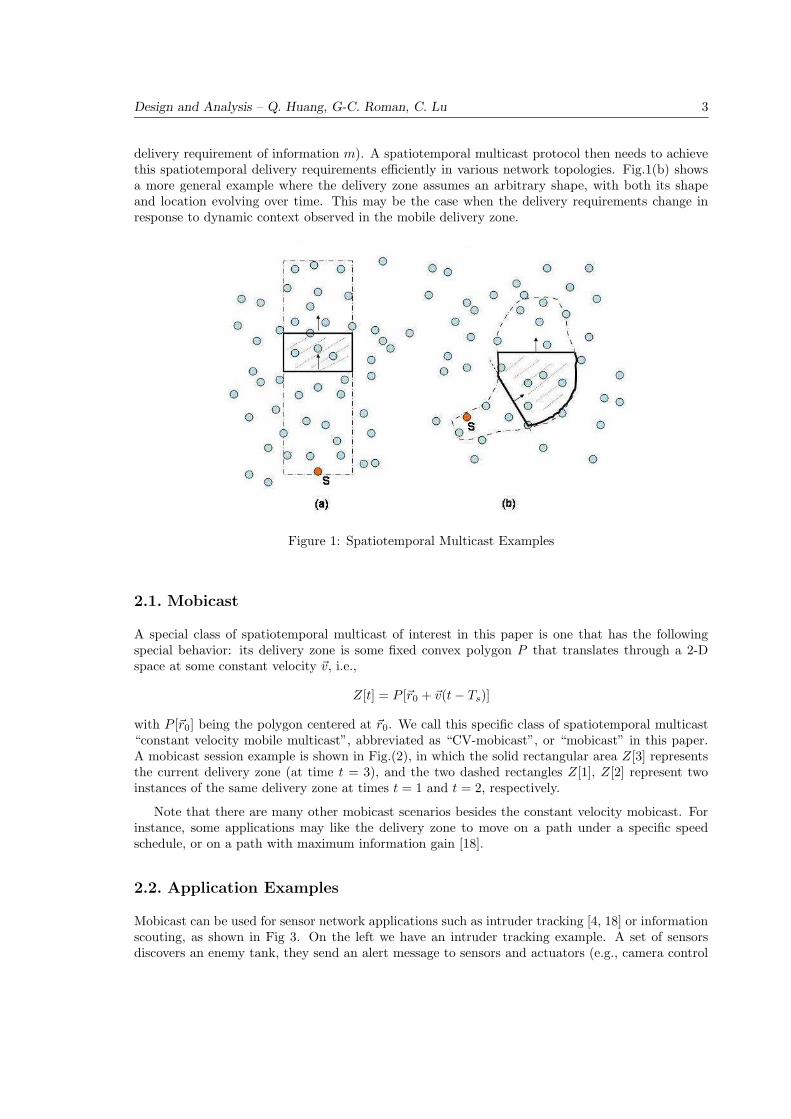
Fig.1 shows two examples of spatiotemporal multicast with different kinds of delivery zones.Fig.1(a) depicts a rectangle-shaped zone (shaded) that moves from the source located at the bottomof the figure to the top. As the delivery zone moves, some nodes enter the zone and some othersleave the zone. The delivery specification of spatiotemporal multicast may require that a node bedelivered the message m at the time the delivery zone reaches the node. Note that the shape andevolving behavior of a delivery zone are defined/specified by mobicast users (for their spatiotemporal


delivery requirement of information m). A spatiotemporal multicast protocol then needs to achievethis spatiotemporal delivery requirements efficiently in various network topologies. Fig.1(b) showsa more general example where the delivery zone assumes an arbitrary shape, with both its shapeand location evolving over time. This may be the case when the delivery requirements change inresponse to dynamic context observed in the mobile delivery zone.

Figure 1: Spatiotemporal Multicast Examples

2.1. Mobicast

A special class of spatiotemporal multicast of interest in this paper is one that has the followingspecial behavior: its delivery zone is some fixed convex polygon P that translates through a 2-Dspace at some constant velocity ~v, i.e.,

Z[t] = P [~r0 + ~v(t − Ts)]

with P [~r0] being the polygon centered at ~r0. We call this specific class of spatiotemporal multicast“constant velocity mobile multicast”, abbreviated as “CV-mobicast”, or “mobicast” in this paper.A mobicast session example is shown in Fig.(2), in which the solid rectangular area Z[3] representsthe current delivery zone (at time t = 3), and the two dashed rectangles Z[1], Z[2] represent twoinstances of the same delivery zone at times t = 1 and t = 2, respectively.

Note that there are many other mobicast scenarios besides the constant velocity mobicast. Forinstance, some applications may like the delivery zone to move on a path under a specific speedschedule, or on a path with maximum information gain [18].

2.2. Application Examples

Mobicast can be used for sensor network applications such as intruder tracking [4, 18] or informationscouting, as shown in Fig 3. On the left we have an intruder tracking example. A set of sensorsdiscovers an enemy tank, they send an alert message to sensors and actuators (e.g., camera control


Figure 2: Mobicast example: A Moving Rectangular Delivery Zone

Figure 3: Tracking and Scouting Applications

units) on the intruder’s expected path to wake them up, alert them, or pre-arm them for bettertracking and actions. This alert message can be sent by a mobicast service, using a delivery zoneof desired size that moves at certain distance ahead of the intruder, with a speed approximatingthat of the intruder’s, thus creating an evolving alert “cloud” just in front of it. The right sideof Fig 3 depicts an information scouting example. A solider is running to the southeast area. Forsafety and/or action efficiency, he would like to know the field information ahead on his path, so asto adjust his action accordingly. His area of interest changes in front of him as he runs. One cansee that this is another natural application scenario for mobicast. The solider can send a scoutingrequest to a delivery zone that moves on his path in front of him. Only the sensors that enterthe delivery zone (receive the scouting message) will pool their currently sensed information andsend aggregated data back to him. The use of mobicast naturally delivers the spatial and temporallocality requirements of information dissemination and gathering exhibited by these applications.

A key observation here is that if the mobile event does not change its motion very often, the


system alert or scouting message does not need to be issued all the time. But rather, one can let themessage roll on its own according to a motion plan. If the mobile event changes or the old mobicastexpires, one can always issue a new mobicast reflecting the new information.

2.3. Specification of Spatiotemporal Delivery Guarantees

As we have pointed out earlier, application developers can encode their spatiotemporal informationdelivery requirements via the delivery zone behavior. The complexity of a mobicast protocol ingeneral depends on the delivery guarantees it is required to achieve. A straight-forward deliveryspecification may demand that once a node α is in a delivery zone Z[t], it receives the informationm immediately. Here we will first try to define and refine this specification formally, and discuss itsfeasibility and implications. Let Ω be the set of all nodes in space, let ~r(j) be the location of nodej, and let D[j, t] denote the fact that j has been delivered the information m at time t. Let the timewhen the mobicast is initiated be Ts. This mobicast delivery property can be formally stated as

〈∀j, t : j ∈ Ω ∧ Ts ≤ t ≤ Ts + T :: ~r(j) ∈ Z[t] =⇒ D[j, t]〉1 (1)

This statement can be interpreted as “During the mobicast session, all nodes inside zone Z at timet should have information m.”

Unfortunately, the delivery property (1) is practically impossible to realize in most wireless adhoc networks. The reasons include:

• First, communication latency is often not negligible in wireless ad hoc networks. This isespecially true in wireless sensor networks where sensor nodes might have a sleeping schedulein order to save energy. Note that (1) implies instantaneous delivery to all nodes at the initialdelivery zone Z[0]. If Z[0] contains a node other than the sender node, it is impossible for thenode to receive information D instantly when considering the communication latency.

• Second, a wireless ad hoc network may be partitioned. A delivery zone, specified by somegeometric property alone, might cover nodes in multiple network partitions, which in turnrenders the delivery impossible.

• Third, we did not put any restrictions on the speed of the delivery zone. One can imaginecases where a user-specified delivery zone moves so fast that it exceeds the maximum deliveryspeed a network can support.

As such, we are forced to weaken the ideal mobicast delivery property in the following practically-minded manner: mobicast satisfies property (1) only after some initialization time tinit on a con-nected network. That is

〈∀j, t : j ∈ Ω ∧ tinit < t ≤ T :: ~r(j) ∈ Z[t] =⇒ D[j, t]〉 (2)

Thus, each mobicast session has two phases. The first, from time 0 to tinit, is an initialization phasein which no delivery guarantee is specified. The second phase, from time tinit to T , is a stable phasein which the strong spatiotemporal guarantee is required. We also implicitly assume the speed ofdelivery zone is smaller than the maximum speed the network can support. (The upper-bound fora feasible speed is addressed by theorem 3 in Section 3)

1The three-part notation 〈op quantified variable : range :: expression〉 used throughout the text is defined as

follows: The variables from quantified variables take on all possible values permitted by range. If range is missing,

the first colon is omitted and the domain of the variables is restricted by context. Each such instantiation of the

variables is substituted in expression producing a multiset of values to which op is applied, yielding the value of the

three-part expression.


2.4. Optimization Concerns

Note that specification (2) addresses only the functional requirement for mobicast, and does notaddress any performance optimization perspectives. Yet, performance is an indispensable dimensionof protocol design. Here we discuss three optimization dimensions for mobicast protocols.

Note that, since communication latency is a random variable, it is impossible for one to delivera message to a node at an exact time. In order to achieve the delivery property (2), one has toconsider the worst case scenario and schedule the delivery of mobicast messages ahead of time.

Let tr(j) denote the time node j receives the mobicast message for the first time, and let tin(j)be the first instant of time j enters the delivery zone. We call the time difference tin(j) − tr(j) the“slack time” associated with the message delivery. It measures how early the message is deliveredto a node with respect to its requisite deadline (to be at the specific node). Note that specification(2) implies that tin is the deadline of message delivery. In general, one would like to have as manyexpected recipients as possible meet the delivery deadline. Let Θ be the set of the “delivery zonenodes” that is defined as the set of all nodes that are expected to receive the mobicast message ina mobicast session. Let Ξ be the set of delivery zone nodes that received the mobicast message onor before the deadline, i.e.,

Ξ ≡ j|(j ∈ Θ) ∧ (tin(j) − tr(j) ≥ 0)

One obvious optimization dimension is to make the initialization phase as short as possible.A smaller tinit means more nodes will meet the delivery deadline. In general, the length of theinitialization time depends on the size of the delivery zone, the network connectivity pattern withinthe region, and the protocol execution behavior. While a mobicast protocol has no control over theformer two factors, it can try to make tinit as short as possible by optimizing its execution strategy.

Another optimization concern for any mobicast protocol is to reduce the overall time intervalbetween the reception of a message and its required delivery to the application, i.e., the slack time.Minimizing the average slack time tslack for all nodes that were ever in the delivery zone improvesthe timeliness of mobicast message delivery, and means less time in “holding” the message before itis needed. Small tslack is also desirable as it potentially leads to less energy consumption and betterlocality in spatial data aggregation. So, a mobicast protocol should seek to minimize the averageslack of the delivery zone nodes:

tslack =

∑j∈Ξ(tr(j) − tin(j))

|Ξ| (3)

where |Ξ| denotes the cardinality of the set Ξ. The ideal case for a mobicast protocol involvesreducing tslack to zero, i.e., a node only receives the mobicast message (from its neighbors) preciselyat the time it enters the delivery zone. Yet, this may not always be possible due to the randomnessof the communication latency.

The third optimization dimension for mobicast is to reduce the total number of retransmissionsneeded for each mobicast session while delivering the spatial and temporal guarantees. This con-cerned is shared with most broadcast and multicast protocols for ad hoc networks.

2.5. Simple Mobicast Solutions

To help see more clearly the complexity of the mobicast, we present first two simple mobicast proto-cols that succeed and fail in different ways. In both protocols, mobicast packets are always marked


by the sender with a description of the packet delivery zone and a life time (for the downstreamnodes to determine their delivery and forwarding behavior).

The first simple mobicast protocol is based on flooding. Once a node receives a mobicast callfrom the application, it floods the mobicast message to the whole network. The rest of the nodesin the network, in addition to participating in the flooding, behave as follows: once a mobicastmessage is received, they schedule the delivery of the mobicast message to the respective interestedapplications at the time when the delivery zone reaches them. If a node finds itself to be never in thedelivery zone of a mobicast, it drops the message after having fulfilled its forwarding responsibility,without delivering the message to application layer. Note that even though this protocol can achievethe spatiotemporal delivery specification (2), it is not desirable in at least two respects. The first isthat the global flooding has a large overhead, especially when the cumulative (union) delivery zonearea is much smaller than the span of the whole network. The second is that the average slack timeof the mobicast reception is higher than necessary, especially when the mobicast delivery zone speedis much smaller than the maximum information propagation speed on the network.

The second protocol examined here employs a hold-and-forward strategy, and only nodes onthe path of the delivery zone will participate. For convenience, we call it the “Delivery-Zone Con-strained” (DZC) protocol. The DZC protocol exhibits minimal delivery overhead and has goodslack time characteristics on “good networks,” but is not entirely reliable. For simplicity, Fig 4shows a mobicast example on a one-dimensional network with a rectangular delivery zone movingat a constant velocity. The DZC protocol works as follows. Once a node receives a new mobicast

Figure 4: Greedy Hold-and-Forward Mobicast Protocol

packet, it first checks if the packet has expired. If not, the node checks to see if it finds itself in thecurrent delivery zone for the packet. If this is the case, the packet is delivered to the applicationimmediately and is forwarded as soon as possible; otherwise, if the node is not currently in thedelivery zone but expects to be in the delivery zone in the future, as the node H in Fig 4, the packetis held and scheduled for delivery and forwarding at the time the delivery zone reaches the node. Inall other cases, nodes will ignore mobicast packets. One can see that the hold and forward behaviorof nodes in front of the running delivery zone makes the packet delivery and forwarding “just-in-time,” and creates a self-sustained mobile message wave. Note that only nodes that find themselvesin the delivery zone path will join the forwarding. This delivery-zone constrained forwarding keepsthe forwarding overhead at a minimum. Yet, the protocol fails to deliver the mobicast message todelivery zone nodes that are not directly connected to the source through a path fully contained inthe area which the delivery zone covers over time. Fig 5 shows such an example. DZC protocol failsto deliver the mobicast message to node X because the nodes outside of the delivery zone do notparticipate in the forwarding process.

From the drawbacks of the DCZ protocol we can see that in order to guarantee mobicast deliveryfor all delivery zone nodes, some nodes that are not in the delivery zone have to participate in message


Figure 5: DZC protocol cannot guarantee delivery

forwarding. An important question is: how to determine who should participate without knowingthe detail of the global network topology? Furthermore, potential holes in the network (as in Fig 5)show that two nodes close in physical space can be relatively far away in terms of network hops.This presents a serious challenge for timely delivery of mobicast messages, i.e., a mobicast protocolneeds to consider potential propagation latency in physical space due to long underlying networkpaths in order to achieve timely delivery across the physical space. In the next section, we furtherinvestigate these challenges under the backdrop of random sensor networks and propose a reliablemobicast protocol.

3. A Reliable Mobicast Protocol

As alluded earlier, a key challenge we want to tackle in this paper is the reliable mobicast delivery,as specified by (2), on networks of arbitrary topology while using only limited information about thenetwork topology. In this section, we explain the key assumptions regarding the network, describethe framework for a reliable mobicast protocol, and offer an analysis and proof of reliability for thisprotocol. Our effort in deriving the protocol yields new insights and concepts useful in the study ofspatiotemporal information dissemination strategies across sensor networks.

3.1. Sensor Network Model

The sensor network model for our protocol is as follows. The network does not have any partition,and all nodes are location-aware, i.e., they know their location ~r in space with reasonable accuracy.The maximum clock-drift among the sensors in the system is small enough to be negligible. All


nodes support wireless communication and are able to act as routers for other nodes. Local wirelessbroadcast is reliable, i.e., once a local broadcast is executed, it will be heard by all its neighborswithin latency τ1.

3.2. The Forward-Zone Constrained (FZC) Mobicast Protocol

In this section we propose a mobicast protocol featuring a “forwarding zone” that cruises in front ofthe moving delivery zone at a certain prescribed distance. Only nodes in the path of the forwardingzone will participate in the mobicast forwarding. We call this protocol the “Forward-Zone Con-strained” (FZC) mobicast protocol. In order to describe the FZC mobicast protocol more concisely,we need to introduce some terminology. The reader is reminded that the delivery zone, specifiedby the application itself, is an area where the delivery of messages to the application takes place.Our protocol creates and uses a “forwarding zone” F [t] that is moving at some distance ahead ofthe delivery zone, as shown in Fig. 6. We call the distance between the forwarding zone and itsassociated delivery zone the “headway distance” (of the forwarding zone). The shape of the forward-ing zone is related to the shape of the delivery zone, and the topology of the underlying network.More specifically, in our protocol, the shape of the forwarding zone is generated from a “seed shape”which we call the “core” of the forwarding zone with a metric of the network topology. The choiceof the headway distance and the size of the forwarding zone is such that it guarantees that all nodesentering the delivery zone will have received the mobicast message in advance, even if some of themare not directly connected (1-hop) to any nodes already in the delivery zone. The forwarding zonelimits retransmission to a bounded space while ensuring that all nodes that need to get the messagewill do so. We will discuss how the forwarding zone is determined in the next section. While nodes

Figure 6: Mobicast example

in a forwarding zone retransmit the mobicast message as soon as they receive it (for the first time),the nodes in front of the forwarding zone enter a “hold-and-forward” state whenever they hear themobicast message. They will retransmit the message only after becoming members of the forwardingzone. As we pointed out earlier, the action of the nodes in the hold-and-forward zone implementsthe “just-in-time” feature of the mobicast delivery policy while keeping the average slack time tslack

small. This behavior results in a virtual “hold-and-forward zone” in front of the forwarding zone,as also indicated in Fig.6.


When a request 〈m,Z[t], Ts, T 〉 is presented to the mobicast service, it constructs and broadcastsa mobicast message to all the neighbors at time Ts. A mobicast packet m contains the followinginformation: a unique message identifier, a delivery zone descriptor, a forwarding zone descriptor, thesession start time Ts, the session lifetime T , and the message data m. The unique message identifieris created from the combination of the location of the source and the time Ts of the request. Thedelivery zone descriptor encodes the original location, the shape of the zone, and its velocity. Theforwarding zone descriptor encodes the shape and the original location of the forwarding zone, whichis computed using some knowledge about the network and the shape of the delivery zone. We willdiscuss in detail the computation of the forwarding zone in later sections.

Upon hearing a mobicast message m at time t.——————————

1.if (m ) is new and t < t0 + T2. if (I am in F[t]) then

3. broadcast m immediately ; // fast forward4. if (I am in Z[t]) then

5. deliver the message data D to the application layer;6. else

7. compute the earliest time tin for me to enter the delivery zone;8. if tin exists and tin < t0 + T9. schedule delivery of data D to the application layer at tin;10. end if

11. end if

12. else

13. compute the earliest time t′ for me to enter the forwarding zone;14. if t′ exists15. if t0 ≤ t′ ≤ t16. broadcast m immediately ; // catch-up!17. else if t < t′ < t0 + T18. schedule a broadcast of m at t′; //hold and forward19. end if

20. end if

21. end if

22. end if

Figure 7: The FZC mobicast protocol

The FZC mobicast protocol is described in Fig.7. While not explicitly shown in the code, thismobicast protocol exhibits two phases in its spatial and temporal behavior. The first is an initializa-tion phase, in which the nodes are trying to “catch-up” with the spatial and temporal demands ofthe mobicast. When a node in the path of the forwarding zone receives a message for the first time,it rebroadcasts the message as soon as possible. This phase continues until a stable forwarding zonethat travels at a certain distance ds ahead of the delivery zone is created.

The second phase is a cruising phase in which the forwarding zone moves at the same velocityas the delivery zone. The protocol enters this phase after the delivery zone and the forwarding zonereach the stable headway distance ds. This cruising effect is achieved by having the nodes at themoving front of the forwarding zone retransmit the mobicast message in a controlled “hold-and-forward” fashion to make the forwarding zone move at the velocity ~v. The initialization and thecruising phases together establish mobicast property (2) with tinit being the time required by theinitialization phase.


In the next section we turn our attention to explaining how the forwarding zone and its stableheadway distance are computed, what is the value of tinit given a specific mobicast request and thespatial properties of the underlying network, and how the protocol delivers on its guarantees.

3.3. Analysis

The key elements in the FZC mobicast protocol (Fig.7) are the forwarding zone and its headwaydistance ds from the delivery zone. As we mentioned earlier, the purpose of the forwarding zone andits headway distance is to ensure that all the nodes entering a delivery zone will receive the mobicastmessage in advance, while minimizing the total number of nodes participating in each mobicastsession.

The shape of the forwarding zone depends on the following three factors: the shape of thedelivery zone, the spatial distribution of the network nodes, and the topology of the network. Fig.8illustrates this point for a rectangle mobicast delivery zone (solid rectangle). The source node Sinitiates a mobicast. For node A to be able to deliver the message (to the respective applicationlayer) when it becomes a member of the delivery zone, it should have received the message by thattime. In scenario Fig.8(a), the message is required to have gone through G (in order for it to reachA). This requires A and G to be in the forwarding zone together at some point in time before Acan receive the message (otherwise, the mobicast message will not be forwarded to A, as A is in a“past” location comparing to G, with respect to the delivery zone velocity direction). On the otherhand, if the network connectivity is “denser,” as in Fig.8(b), the width of forwarding zone (e.g.,the dashed rectangle, comparing to the one in Fig.8(a)) can be relatively smaller. Furthermore, in

Figure 8: Spatial and connectivity configuration of the network influence the size of forwarding zone

Fig.8(a) the height of the forwarding zone has to be bigger than the height of the delivery zone soas to include D. Otherwise, nodes A,B and C will be effectively partitioned from the rest of thenodes in the network, because node D will not participate in the routing process. This is just onespecial example with an ad hoc choice of forwarding zone. The question we would like to address is,in an arbitrary sensor network, how to determine the forwarding zone and its headway distance fora specific delivery zone.


We found that the minimum size, shape, and headway distance for a mobicast protocol thatprovides a strong spatial and temporal delivery guarantee (in the presence of an arbitrary networktopology) depend on two network metrics we call “∆-compactness” and “Γ-compactness.” Thesetwo metrics capture the spatial and temporal information propagation properties of sensor networksin Euclidean space, respectively, and are related to the following three distance metrics between twonodes i and j in a network:

• Euclidean distance, denoted as d(i, j);

• Shortest network distance, in terms of smallest network hops, denoted as h(i, j);

• S2 distance, defined as smallest Euclidean path length among the set of shortest networkpaths between nodes i and j, denoted as d(i, j).

Next we formalize these network compactness metrics and discuss how they relate to the compu-tation of the forwarding zone and its headway distance. Then we show that our protocol provides thedesired spatiotemporal guarantees given the proper choice of the forwarding zone and its headwaydistance.

3.3.1. Computing the Forwarding Zone. In order to describe how the minimum forwardingzone can be determined for a specific delivery zone in an arbitrary network, we first introduce thedefinition of the “∆-compactness” measure for the network.

∆-compactness. Given a geometric graph/network G(V,E), ∆-compactness seeks to quantifythe relation between the Euclidean distance and the S2 distance among network nodes. We denotethe Euclidean distance to shortest path distance ratio between two nodes i and j as δ(i, j), i.e.,

δ(i, j) =d(i, j)

d(i, j)(4)

We call δ(i, j) the pairwise “∆-compactness” between nodes i and j. The ∆-compactness of ageometric graph G(V,E) is defined as the smallest ∆-compactness of all node pairs of the network:

δ = mini,j∈V

δ(i, j) (5)

Note that ∆-compactness has a close relation with the terms “dilation”[9], “spanning ratio”[3],and “stretch-factor”[21] used in the graph and computational geometry community. “Dilation” isdefined as the maximum ratio between Euclidean path distance and geometric distance, while ∆-compactness is defined as minimum ratio between the geometric distance and the correspondingS2 distance. They have more than an inverse relationship. For instance, for nodes A and B inFig 9, path ACB contributes to the computation of ∆-compactness while path ADEB contributesto the computation of dilation. The reason is that ∆-compactness is computed on the set of shortestnetwork paths (path of minimum hops) only, while dilation is computed on the set of all paths.Path ADEB has 3 hops and is not a shortest network path between A and B, even though it isa shortest Euclidean network path between them. (As a result, the ∆-compactness of this graphis

√2 = 1.414, while the dilation is 3/

√5 = 1.342). For convenience, we will call the inverse of

∆-compactness ∆-dilation .

Theorem 3.1. Let i, j be any two nodes in a network with ∆-compactness δ. Let E(i, j, δ) be anellipse using i, j as two foci and with eccentricity δ. There is at least one shortest path between iand j inside the ellipse E(i, j, δ).


Figure 9: Dilation and ∆-compactness

Proof: We prove this theorem by contradiction.

Assume the theorem is not true. There must be at least one pair of nodes i and j, whose shortestpaths all have at least one vertex outside the ellipse E(i, j, δ). Using the fact that for all points kon the ellipse, d(i, k) + d(j, k) = d(i, j)/δ, it is easy to prove in this case

d(i, j) >d(i, j)

δ

that is

δ >d(i, j)

d(i, j)

this directly contradicts the definition of ∆-compactness (5).

This theorem is very useful for limiting the forwarding region while guaranteeing point to pointmessage delivery in a geometric network. In our case, this metric helps us decide the shape and sizeof the forwarding zone, which turns out to relate to a notion called “k-cover”.

K-cover. We introduce the notion “k-cover” of a polygon to simplify the mathematical de-scription of the forwarding zone. The k-cover of a convex polygon P is defined as the locus of allpoints p in the plane for which two points q and r in the polygon P exist such that

d(p, q) + d(p, r) ≤ kd(q, r) (6)

where the d(x, y) is the distance between points x and y.

Theorem 3.2. Let i, j be two nodes in a ∆-compact network, and assume that i and j are insidea convex polygon P . The 1

δ -cover of P contains at least one shortest path between i and j.

Proof: (The proof is similar to that of theorem (3.1), and thus omitted.)

One may view an ellipse to be a special case of k-cover. An ellipse of eccentricity e is a 1e -cover of

the line segment between the two foci of the ellipse. In other words, the k-cover is a generalizationfor the ellipse.


The Forwarding Zone. Given a mobicast delivery zone of convex shape P , if the mobicastis executed on a network with ∆-compactness value δ, then we choose the shape of the forwardingzone’s core to be P and the shape of the forwarding zone to be the 1

δ -cover of its core.

Corollary 3.1. Let i, j be two nodes in the core of a forwarding zone on a network whose ∆-compactness is δ. The forwarding zone contains at least one shortest path between i and j.

Proof: This results from theorem (3.2) and the construction of the forwarding zone.

3.3.2. Computing the Stable Headway Distance. The headway distance of the forwardingzone is a way to tell the protocol how far ahead to prepare the message delivery in order not to missthe delivery deadline as a result of some unexpected distortions on related network paths. It shouldbe intuitively clear that a network with more “indirect” network paths requires a longer headwaydistance than one whose paths are more “direct.” In order to capture this notion more precisely, weintroduce the “Γ-compactness” metric.

Γ-compactness. Γ-compactness quantifies the relation between the shortest network distanceand the Euclidean distance among the nodes in a geometric network. We define the Γ-compactnessof a geometric graph G(V,E) to be the minimum ratio of the Euclidean distance to the shortestnetwork distance between any two nodes in the network, i.e.,

Γ = mini,j∈V

d(i, j)

h(i, j)(7)

Intuitively, if a network’s Γ-compactness value is γ, then any two nodes in the network at a distanced have a shortest path no greater than d/γ hops.

Theorem 3.3. Let N be a network with a Γ-compactness value γ and let τ1 be its maximum 1-hopcommunication latency. The lower bound of the maximum message delivery speed over the spaceon N is γ

τ1

.

Proof: Let d(i, j) be the distance between two arbitrary nodes i and j in the network. We knowthat the shortest network path h between the two nodes is bounded by

h(i, j) ≤ d(i, j)

γ(8)

We also know that a message sent from one node to another node h-hops away takes no longer thanhτ1 if each intermediate node forwards the message immediately after receiving it. Let t be the timeit actually takes for the message to go from i to j. In this case we have

t ≤ h(i, j)τ1

From this we know that the average speed v of this information propagation over distance d(i, j) is

v =d(i, j)

t≥ d(i, j)

hτ1≥ γ

τ1(9)

Note that the bound γτ1

is not dependent on d(i, j). This inequality (9) is true for any two nodesin any network with Γ-compactness value γ, when all nodes in the network relay the message as


soon as possible. That means γτ1

is a lower bound on the maximum spatial message delivery speedon networks with Γ-compactness value γ.

Theorem (3.3) states that, given a geometric network, there is a clear limit to how fast spa-tiotemporal information dissemination can be achieved. For instance, given a geometric networkwith Γ-compactness value γ, one can not guarantee the delivery zone to move at a speed higher thanγτ1

in all areas.

3.3.3. The Headway Distance. The stable headway distance ds must be large enough toensure that when the delivery zone reaches a node, the message has been received already, i.e.,tin > tr is achieved for all nodes.

Theorem 3.4. Let Sd be the maximum distance between the boundary points of the delivery zone,let v be the speed of the delivery zone, let τ1 be the 1-hop maximum network latency of the networkand let γ be its Γ-compactness . If we let ds = vτ1bSd

γ c, then all the nodes in the core of theforwarding zone will have received the the mobicast message by the time delivery zone reachesthem, assuming there is at least one node in the core that has received the message.

Proof: Let us consider a snapshot of the mobicast at some time t and the core of the currentforwarding zone. Let i denote the node in the core that already has the message. Its distance to allother nodes in the core is less than Sd, because Sd is the maximum size of the delivery zone, as wellas that of the core. The longest of the shortest network paths from i to all other nodes in the coreof is less than bSd

γ c hops. In turn, at most τ = bSd

γ cτ1 time is needed for a message to traverse thecore if all nodes forward the message as soon as possible. We can conclude that after τ , all nodesin the core of the forwarding zone will get the message, because in the protocol all nodes inside theforwarding zone forward mobicast messages in as soon as possible, and there is always a shortestpath inside the forwarding zone for any two nodes inside its core. Since the speed of the deliveryzone is v, a distance ds = vτ1bSd

γ c takes exactly τ time to be traversed.

Hence, it is true that all the nodes in the core of the forwarding zone will have received the themobicast message when the delivery zone reaches them, assuming at least one node in the core hasreceived the message and given the headway distance ds = vτ1bSd

γ c.Given the headway distance d and the shape F of the forwarding zone, a node can easily determine

the current forwarding zone using velocity v, current time t, sending time t0 and the source locationr0. Note that t0 and r0 can be obtained from the mobicast protocol message header.

3.3.4. Duration of Initialization Phase. As we pointed out earlier, it is in the cruisingphase that the mobicast protocol guarantees on-time delivery. In the initialization phase, the timingconstraint of mobicast is realized in a best-effort manner. It is possible that in the initializationphase, some nodes may not get the messages in time. The initialization phase continues until onenode inside the core of the forwarding zone that is ds ahead of the delivery zone receives the mobicastmessage. From theorem (3.4), we know that after this, the timing constraint of mobicast is alwayssatisfied.

The time (tinit) it takes for the mobicast protocol to enter the cruising phase is related to thestable distance needed, the delivery zone speed, and the maximum admissible spatial propagationspeed of the network.

Theorem 3.5. Let ds be the required headway stable distance between the forwarding zone and thedelivery zone. Let w be the width of the delivery zone. Let v be the speed of the delivery zone andu be lower bound on the maximum message delivery speed achievable in the network. The mobicast

protocol initialization time tinit is no greater than (ds+w)u−v


Proof: In the protocol, the nodes in the forwarding zone and between the forwarding zone and thedelivery zone retransmit the message immediately the first time they receive it. As such, the protocolachieves a maximum message propagation speed vmax in this phase. This message propagation speedrelative to the delivery zone is vmax − v. Meanwhile, the end-to-end distance between the deliveryzone and the core of the forwarding zone is ds + w, which can be covered by a message propagatingat the speed vmax − v in t = ds+w

vmax−v time. When a message from the delivery zone reaches the coreof the forwarding zone ds distance ahead of the delivery zone, by definition the initialization phaseis over. Hence we have

tinit ≤ t =ds + w

vmax − v≤ (ds + w)

u − v(10)

in the above we also used u < vmax, which by definition is true.

The Spatiotemporal Guarantees of the Protocol. The spatiotemporal guarantees of theFZC mobicast protocol (7) are addressed by the following theorem:

Theorem 3.6. If at any instant of time in a mobicast session, its (user-defined) delivery zone coversat least one node in the network, our mobicast protocol delivers property (2) with

tinit ≤vτ1bSd

γ + wcγτ1

− v

.

Proof: If a delivery zone covers at least one node in the network at any instant of time, thenwhenever the last node in a delivery zone is leaving a delivery zone, there must be another nodeentering it. The same is true for the core of the forwarding zone, because it is of the same shapeas the delivery zone and moves on the same path. If at one point in time, a node in the core ofthe delivery zone has received the mobicast message, it will always be able to pass the message onto all others nodes on the path because our protocol and the way we choose the forwarding zoneguarantees that if two nodes ever appear together in the same core of the forwarding zone, onehaving the message means the other will get it too.

By using theorems (3.4) and (3.5), it is easy to see that property (2) is satisfied.

3.4. New Questions

So far we have proved that FZC mobicast protocol is able to achieve the strong mobicast deliveryguarantees specified in Section 2 given a proper choice of the forwarding shape and its headwaydistance, under a set of necessary assumptions. Note that for the FZC mobicast protocol, theforwarding zone size is the 1

δ -cover of the delivery zone. A small value for ∆-compactness impliesa relatively big mobicast overhead, defined as the number of nodes participating in the mobicastmessage forwarding. Note also that in the previous protocol, the network compactness values areused because of the need for strong delivery guarantees, captured by the concern with the worstcase path distortion in a network rather than the average case. Several new questions arise: (1)What is the typical compactness value for common sensor networks? (2) Can we make a networkmore compact to support better spatiotemporal communication? (3) The previous protocol used theworst case compactness among all paths, as it was geared towards 100% delivery guarantee. Thischoice might be pessimistic if the worst case is rare. How will an optimistic choice of forwarding zoneperform in reality? (4) Can we use a local notion of compactness and can the mobicast session andthe forwarding zone be adaptively adjusted to the local compactness values? Next, we will turn ourattention to addressing the first three questions. An investigation of the last question is reported ina separate work [11].


4. Properties of Random Networks

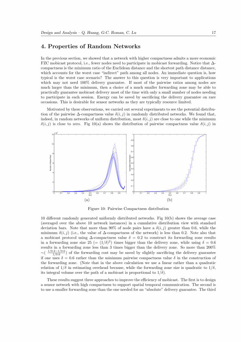
In the previous section, we showed that a network with higher compactness admits a more economicFZC mobicast protocol, i.e., fewer nodes need to participate in mobicast forwarding. Notice that ∆-compactness is the minimum ratio of the Euclidean distance and the shortest path distance distance,which accounts for the worst case “indirect” path among all nodes. An immediate question is, howtypical is the worst case scenario? The answer to this question is very important to applicationswhich may not need 100% delivery guarantee. If most of the pairwise ratios among nodes aremuch larger than the minimum, then a choice of a much smaller forwarding zone may be able topractically guarantee mobicast delivery most of the time with only a small number of nodes needingto participate in each session. Energy can be saved by sacrificing the delivery guarantee on rareoccasions. This is desirable for sensor networks as they are typically resource limited.

Motivated by these observations, we carried out several experiments to see the potential distribu-tion of the pairwise ∆-compactness value δ(i, j) in randomly distributed networks. We found that,indeed, in random networks of uniform distribution, most δ(i, j) are close to one while the minimumδ(i, j) is close to zero. Fig 10(a) shows the distribution of pairwise compactness value δ(i, j) in

0 0.1 0.2 0.3 0.4 0.5 0.6 0.7 0.8 0.9 10

2

4

6

8

10

12x 104

δ(i,j)

Num

ber o

f Nod

e P

airs

0 0.1 0.2 0.3 0.4 0.5 0.6 0.7 0.8 0.9 10

0.1

0.2

0.3

0.4

0.5

0.6

0.7

0.8

0.9

1

δ(i,j)

Cum

ulat

ive

Dis

tribu

tion

(a) (b)

Figure 10: Pairwise Compactness distribution

10 different randomly generated uniformly distributed networks. Fig 10(b) shows the average case(averaged over the above 10 network instances) in a cumulative distribution view with standarddeviation bars. Note that more than 90% of node pairs have a δ(i, j) greater than 0.6, while theminimum δ(i, j) (i.e., the value of ∆-compactness of the network) is less than 0.2. Note also thata mobicast protocol using ∆-compactness value δ = 0.2 to construct its forwarding zone resultsin a forwarding zone size 25 (= (1/δ)2) times bigger than the delivery zone, while using δ = 0.6results in a forwarding zone less than 3 times bigger than the delivery zone. So more than 200%

∼( 1/0.2−1/0.61/0.6 ) of the forwarding cost may be saved by slightly sacrificing the delivery guarantee

if one uses δ = 0.6 rather than the minimum pairwise compactness value δ in the construction ofthe forwarding zone. (Note that in the above calculation we use a linear rather than a quadraticrelation of 1/δ in estimating overhead because, while the forwarding zone size is quadratic to 1/δ,its integral volume over the path of a mobicast is proportional to 1/δ).

These results suggest three approaches to improve the efficiency of mobicast. The first is to designa sensor network with high compactness to support spatial temporal communication. The second isto use a smaller forwarding zone than the one needed for an “absolute” delivery guarantee. The third


is to use a protocol that adapts to the local compactness conditions rather than the global one. Inthis paper, we focus on examining the first two approaches, with some preliminary results about thethird approach. Investigation of the first approach is presented next. An investigation of the secondapproach appears in section VI. The third approach is presented in a separate publication [11].

4.1. Impact of Node Density on Network Compactness

As we pointed out earlier, for a specific delivery zone, the more “compact” a network is, the smallerthe forwarding zone needs to be. An immediate question is, can we design the sensor network soas to make its ∆-compactness value as close to the maximum value of one as possible? Since wewant to continue with the random distribution assumption, there is only one design dimension left:the sensor node density. Note that we define sensor density as the average number of immediatenetwork neighbors for each node, rather than number of nodes in a unit area.

Intuitively, the higher the sensor density, the “better” connected the sensor network is and thelarger the corresponding network ∆-compactness is. To verify this observation, we designed thefollowing experiment. We scatter 800 sensors uniformly distributed in a 1000x400 rectangular areaand select only configurations which are not partitioned for a communication range of 35. (Note thatbecause of random distribution, the network is sometimes partitioned. 35 is close to a critical rangefor connectivity in our experimental configuration). For the surviving configurations, we computethe values of ∆-compactness assuming communication range valuea between 35 and 90. Note that inthis experiment we chose to vary the communication range rather than to vary node density directly(by adding more nodes to the area). The reason we chose to vary the communication range as amechanism to vary the relative sensor density is because this does not change the actual locationconfiguration of the sensors in the experiment and, in turn, makes the corresponding compactnessvalue comparison more meaningful.

The above procedure was repeated for five different configurations and the results (average valuesand standard deviations) are presented in Fig 11. Fig 11(a) shows the average (across the 5 runs)

30 40 50 60 70 80 90 1000

2

4

6

8

10

12

Communication Range (meters)

Net

wor

k D

ilatio

n

Area: 1000 X 400Number of Nodes: 800Spatial Dsitribution: uniform

max dilation

max dilation of 99%

5 10 15 20 25 30 35 40 45 50 550

2

4

6

8

10

12

Net

wor

k D

ilatio

n

Average Number of Neighbors

Area: 1000 X 400Number of Nodes: 800Spatial Dsitribution: uniform

max dilation of 99%

max dilation

(a) (b)

Figure 11: (a)∆-Dilation vs Range, (b)∆-Dilation vs Average Number of Neighbors

∆-Dilation (defined as the inverse of ∆-compactness ) versus the change of communication range.Fig 11(b) shows a corresponding figure with the average node degree as the x-axis.

The results show that the network compactness indeed increases when the node density increases.But surprisingly, there appears to have a saturation point at a moderate density. The network


exhibits a rapid increase in compactness (rapid decrease in ∆-dilation ) when the average number ofneighbors changes from 8 to 15 and then starts to saturate. This appears to be an area to increasethe compactness of the network with highest efficiency for these randomly distributed networks.This may provide a good heuristic for deploying mobicast/communication friendly sensor networks.For instance, if one wants to monitor a area of 1000x1000 square meters using sensors of averagerange 50 meters, the total number of sensors should be about 1000×1000

π502 × 15 = 1910 for a randomscattering deployment method. One can also see that after a certain threshold (15 ∼ 20 neighborsin this case), increasing the node density no longer introduces much benefit in terms of improvingcompactness.

In addition, we also examined the value of the majorities of the pairwise ∆-compactness and howthey change with node density. The lower curve in Fig 11(a) and (b) shows how the lower bound ofthe top 99% of the δ(i, j) of the network changes with node density. One can see that the occurrenceof the lower extreme compactness value is a rare event. This further suggests that an optimisticchoice of k-cover for the forwarding zone is a good mobicast strategy in practice.

5. Optimistic Mobicast

To verify our observations about the potential benefit of optimistic mobicast on random networkswith uniform distribution, we implemented an extended mobicast protocol on the ns-2 networksimulator. Our implementation was extended with a mode to let the user specify the parameter(delta) for determining the forwarding zone. This allows us to test the trade-off between the message2

forwarding cost and the delivery guarantee.

The header of our mobicast protocol packet contains the following information:

- message type - delivery zone size (radius)- sender packet sequence number - delivery zone velocity (x and y components)- sender location (x and y coordinates) - delta factor- sending time - gamma factor- message lifetime

Our protocol only provides support for a circular delivery zone. We also assume that the initialdelivery zone is centered at the sender. One may augment the header with the information about theinitial delivery zone center to allow applications to explicitly set the initial delivery zone location.Because this is not essential for our validation and verification test purposes, we simply default thesender location as the center of the initial delivery zone.

The mobicast protocol is depicted in Fig 16 (modified from Fig 7, with additional compactnessinformation processing). In this paper we omit the detail about the geometric computation involvedin determining if and when a node is in a forwarding zone and delivery zone, as it is not conceptuallyessential. The mobicast protocol also maintains a transient message cache (it is periodically cleanedby throwing out expired messages).

To minimize the dependence of simulation results on the network configuration used, our experi-ments were run on five different connected network configurations generated via uniformly distribut-ing 800 sensor nodes on a 1000x400m area. Fig 12(b) shows one such configuration example used.(the network connectivity pattern is shown Fig 12(a)). One node close to the left is chosen as themobicast sender. Our results are averaged over multiple runs on five network configurations. For all

2Note that we use “packet” and “message” interchangeably here. In the simulation, we only deal with cases where

a mobicast message can be fit in one mobicast packet.


(a)

(b)

Figure 12: Optimistic Mobicast Simulation Example

runs, the delivery zone velocity is 40m/s, from left to right, and each mobicast session has a lifetimeof 20s. For all the configurations used, the critical communication range for all the nodes to form aconnected graph is between 30 to 35 meters. We chose the delivery zone radius to be 45 meters.

We designed two sets of experiments. The first one intended to investigate how mobicast deliveryratio and forwarding overhead changes with the size of the forwarding zone on these uniformlydistributed networks. Delivery ratio is defined as the percentage of delivery-zone nodes (those thatare in the virtual delivery zone at some point of time during a mobicast session) that actuallyreceived the mobicast message. Forwarding overhead is defined as the number of extra messagetransmissions per node delivery, i.e., the total number of retransmissions divided by the numberof delivery zone nodes that actually received the message. Fig 13(a) shows the simulation resultsof delivery ratio versus the normalized forwarding zone size (the actual k used in forwarding zonecomputation.) One can see the delivery ratio improves when the forwarding zone becomes bigger.The high variance in delivery ratio value is due to random distribution of holes across differentconfigurations, which causes each mobicast session to stop prematurely at different locations acrossdifferent configurations. The limited number of network configurations used also contribute to this.Fig 13(b) shows how the forwarding overhead changes with the forwarding zone factor. Clearly themessage forwarding overhead increases almost linearly with the increase of forwarding zone factor.

The second set of experiments were designed to investigate how the delivery ratio is affectedwhen the network becomes more compact. Due to the limited scalability of ns-2, we again use thechange of the communication range to change compactness, rather than by adding more nodes. Inthe experiment, the delivery zone radius used is 45 meters. The communication radius varies from35 to 45 meters. We collected results from multiple runs of mobicast using different forwarding zonefactors over the five configurations and results are summarized in Fig 14.

From these results we can see that indeed the delivery ratio increases when the node density


0.5 1 1.5 2 2.5 3 3.5 40

0.2

0.4

0.6

0.8

1

Forwarding Zone Factor

Del

iver

y R

atio

0.5 1 1.5 2 2.5 3 3.50

0.5

1

1.5

2

2.5

3

Forwarding Zone Factor

Nor

mal

ized

For

war

ding

Ove

rhea

d

(a) (b)

Figure 13: (a) Delivery ratio vs Forwarding Zone Size; (b) Normalized Forwarding Overhead vsForwarding Zone Factor

R \ δ 1.0 0.9 0.8 0.7 0.6 0.5 0.4

35 0.69± 0.29 0.78± 0.29 0.80± 0.28 0.90± 0.21 0.90± 0.21 0.99± 0.10 1

40 0.90± 0.21 0.90± 0.21 0.90± 0.21 1 1 1 1

45 0.998± 0.003 1 1 1 1 1 1

Figure 14: Delivery ratio v.s. node density and forwarding size

increases, and when the size of the forwarding zone increases. Again the high variance in the valueis due to random distribution of holes across different configurations and each mobicast sessionstops prematurely at different locations across different configurations. These results also in a sensedemonstrate that the forwarding zone in the FZC protocol (based on the value of worst case networkcompactness) is indeed sufficiently large to guarantee the reliable delivery on a connected networkof random topology.

In our simulation, we also examined the timeliness of mobicast delivery on these networks. Morespecifically, we wanted to see how far ahead a node received the mobicast message before enteringthe delivery zone (or how late after entering the delivery zone). Fig 15 shows one typical result of amobicast session, when the communication range is 35m, the delivery zone radius is 45m, δ is 0.7, ds

is 0, and the mobicast speed is 40m/s. Fig 15(a) shows the mobicast packet reception time relativeto the sending time, for all the nodes that were ever in the delivery zone. The solid line is theexpected reception deadline for nodes in each location, i.e, the first time they are expected to enterthe delivery zone. The star dotted line is the actual reception time of the mobicast packet for eachnode. For comparison, we also included a simulation result (the diamond dotted line) of a spatialmulticast on the same path with “as soon as possible” delivery. (Note that in this case the spatialpropagation speed exceeds 1600m/s, i.e., 800m is traversed in less than half a second). We canclearly see the temporal locality property of mobicast. The packet reception time is very close to thedeadline specified by the delivery zone semantics. These results also suggest the benefit of mobicastover a more conventional spatial multicast like geocast, which assume implicit as-soon-as-possibletemporal delivery semantics, i.e, using mobicast one can control information propagation speedto better satisfy application needs while without overwhelming spatiotemporally unrelated nodes.We believe this “just-in-time” delivery nature of mobicast is a powerful mechanism for resourceutilization optimization for related applications in sensor network.


0 100 200 300 400 500 600 700 800 900 1000−2

0

2

4

6

8

10

12

14

16

18

20

Location of Nodes

Rec

eptio

n Ti

me

S

Delivery deadline Mobicast velocity: 40m/sASAP Spatial Multicast

0 100 200 300 400 500 600 700 800 900 10000

2

4

6

8

10

12

14

16

18

20

Location of Nodes

Sla

ck T

ime

S

Mobicast velocity: 40m/sASAP Spatial Multicast

(a) (b)

Figure 15: Slack Time of Mobicast Delivery

Upon hearing a optimistic mobicast message m at time t.1.if (m ) is new and t < T2. cache this message3. if the value of the delta field is zero4. use local knowledge of delta for later computation5. else

6. use the value in the packet for later computation7. end if

8. if (I am in current forwarding zone F[t]) then

9. broadcast m immediately ; // fast forward10. if (I am in current delivery zone Z[t]) then

11. deliver the message data D to the application layer;12. else

13. compute the earliest time td[in] for me to enter the delivery zone;14. if td[in] exists and td[in] < T15. schedule delivery of data D to the application layer at tin;16. end if

17. end if

18. else

19. compute the earliest time tf [in] for me to enter the forwarding zone;20. if tf [in] exists21. if t0 ≤ tf [in] ≤ t22. broadcast m immediately ; // catch-up!23. else if t < tf [in] < T24. schedule a broadcast of m at t′; //hold and forward25. end if

26. end if

27. end if

28. end if

Figure 16: Optimistic Mobicast Protocol


6. Discussion

For reliable mobicast, we introduced two network compactness metrics to help us choose the rightforwarding zone and its headway distance for a given delivery zone so as to achieve the mobicastdelivery guarantee without unnecessary flooding. These compactness values must to be computedfor supporting the FZC mobicast protocol. Calculating them involves computing the shortest pathand Euclidean distances of each pair of nodes in a given network. The all-pair shortest path of agraph G(V,E) can be computed in O(V E log V ) time by using Johnson’s algorithm [7]. All-pairdistance can be computed in O(V 2) time. Therefore, we can compute the Γ-compactness of thegraph in O(V E log V ) time. ∆-compactness can also be computed in O(V E log V ) time. It is notfeasible for individual sensor nodes to compute these values in a large network. In practice, one mayhave a central server collect all the location and connectivity information, do the computation anduse one broadcast to inform all the nodes this value. However, for the local compactness values, itis possible for the sensor nodes to compute the metric values as they involve only a relatively smallnumber of nodes in their respective neighborhood.

While we chose the shape of the forwarding zone to be a 1δ -cover of the shape of the delivery

zone, this was done only for the purpose of analysis. Computing an exact k-cover for an arbitrarypolygon P can be difficult. Yet one can always choose some approximation techniques such as usingthe k-cover of P ’s bounding box or bounding circle, which is computationally much simpler, butstill has the required property (a shortest path between two nodes inside a specific instance of thedelivery zone exists in the cover). The tradeoff is that the resulting forwarding zone is bigger thannecessary, and thus may entail more re-transmissions for the same delivery goal. We should notethat in the FZC protocol the forwarding zone only needs to be computed once by the sender. Thenodes that receive the mobicast message only need to translate the forwarding zone with respect totheir distances from the sender.

An important aspect of mobicast is that applications have control over the velocity of the in-formation dissemination over the space. This brings many new spatial and temporal coordinationand interaction possibilities across a network. For instance, an application might use a mobicast tosend some information to the east at a speed of 40 miles per hour. One second later, it may find achange in that information, (e.g., there is a change in the intruder’s expected path) and may want tosend the new information and stop further propagation of the old information in the network. Notethat stopping previous information dissemination is impossible in conventional protocols which haveexplicit or implicit “as-soon-as-possible” delivery semantics. Yet, in mobicast, a “stop that mes-sage” message can be sent at a much higher speed, say 120 miles per hour, (or even more than 1000miles per hour which we found possible in our simulation), with a same-size delivery zone along theprevious path. Clearly, this new mobicast recall message can easily catch up with its target messagewhich propagates at a much lower speed.

As spatiotemporal protocols are relatively new, there are many research questions waiting tobe answered. For instance, our ns-2 simulations are run without background traffic. When thereis background traffic, the one-hop latency will change and will have a higher variance. Also, morecollisions will happen and more packets will be lost. How background traffic will affect the deliveryratio and timeliness of the spatiotemporal protocols and how the protocols should be adjustedaccordingly are questions we hope to answer in the near future.

Furthermore, for simplicity of presentation, our protocol essentially carries out flooding insidethe forwarding zone. If the nodes have an accurate picture about the locations of their one-hopor two-hop neighbors, one can reduce the number of re-transmissions by using this knowledge in amanner similar to techniques proposed for improving broadcast efficiency [24, 25]. In a probabilisticguarantee scenario, one may also use probabilistic retransmission-reduction techniques such as theone proposed in [23]. A review of these and other related methods can be found in [27]. Our


protocol, by only using the compactness values of the network, tries to use minimum number of bitsto capture the relevant topology. If the nodes have local knowledge about the network topology inthe neighborhood, (e.g., know the locations of all nodes within certain distance) more communicationefficient mobicast protocols can be designed.

Finally, while we are focusing on constant velocity mobicast in this paper, the concept of spa-tiotemporal multicast in general applies to a much wider set of spatiotemporal constraints. Thedelivery zone can exhibit any evolving characteristics as long as it is sustainable by the underlyingsystem. While they may all require ideas similar to the notion of forwarding zone and headwaydistance to maintain the spatiotemporal properties inherent in mobicast, different types of deliv-ery zones may require different protocol handling details. Classification of a useful set of mobicastdelivery zone scenarios and the design of the corresponding mobicast protocols are also importantelements in our future work.

7. Related Work

Mobicast is motivated by the need for coordination activities related to moving entities in the physicalenvironment. In [5], Cerpa et. al. proposed a Frisbee model in which an active sensing zone movesthrough the network along with the target. [16] and [6] proposed several data service protocolsfor improving the accuracy of distributed sensing in mobile environments. Both protocols entailcommunication schemes that push information about the object to the nodes close the projectedlocation of the object in the future. The EnviroTrack group management protocol [1] dynamicallycreates and maintains a group that tracks mobile entities in the environment. However, neitherof the aforementioned projects include communication mechanisms geared toward meeting explicitspatiotemporal constraints related to mobility. Mobicast can be viewed as complimentary to theseprojects by providing a convenient underlying communication mechanism that allows applicationsto push information with specified spatiotemporal requirements.

The idea of disseminating information to nodes in a geographic area is not new. Navas andImielinski proposed geographic multicast addressing and routing ([12, 22]), dubbed “geocast,” forthe Internet. They argued that geocast was a more natural and economic alternative for buildinggeographic service applications than the conventional IP address-based multicast addressing androuting. In a geocast protocol, the multicast group members are determined by their physicallocations. The initiator of a geocast specifies an area for a message to be delivered, and the geocastprotocol tries to deliver the message only to the nodes in that area. Ko and Vaidya investigatedthe problem of geocast in mobile ad hoc networks [15] and proposed to use a “forwarding zone” todecrease delivery overhead of geocast packets. Other mechanisms A([26, 17, 2]) have been proposedto improve geocast efficiency and delivery accuracy in mobile ad hoc networks. Zhou and Singhproposed a content-based multicast [28] in which sensor event information is delivered to nodes insome geographic area that is determined by the velocity and type of the detected events. Whiledifferent in style and approach, all these techniques assume the delivery zone to be fixed. They alsoassume the same information delivery semantics along the temporal domain, i.e., information is tobe delivered “as soon as possible.” However, local coordination often requires just-in-time deliveryin sensor networks.

Data aggregation is an important information processing step in sensor networks. Several tech-niques have been proposed to support data aggregation in sensor networks. For example, both di-rected diffusion ([14, 13]) and TAG [20] allow data to be aggregated on their route from the sourcesto a base station. No explicit local coordination is supported by these techniques. LEACH [10]organizes sensors into local clusters where each cluster head is responsible for aggregating the datafrom the whole cluster. However, there is no notion of mobility and the clusters do not move in space


following a physical entity. In contrast, supporting local coordination for mobile physical entities isa primary goal of mobicast.

8. Conclusion

Spatiotemporal multicast represents a new multicast paradigm for disseminating information whichhas intrinsic spatial and temporal value. Mobile multicast is a special case of spatiotemporal multi-cast which has a promising application potential in sensor networks. To demonstrate the feasibilityof mobicast, we developed a protocol and explored its ability to meet strong spatiotemporal guar-antees. The key element in the protocol is a dynamic forwarding zone moving ahead of the deliveryzone. Furthermore, we introduced two new notions of network compactness and proved several re-lated theorems useful in the analysis of information propagation in wireless sensor networks. Usingthese results we were able to determine the shape of the forwarding zone and the headway dis-tance needed in theory for our protocol to ensure strong multicast delivery guarantees in space andtime while keeping retransmission overhead and average slack time small. The strong spatiotem-poral guarantee differentiates mobicast from existing multicast protocols. We also investigated thenetwork compactness properties of randomly distributed sensor networks and their implication onperformance of mobicast protocols. We found the distribution of values for the compactness metricin randomly distributed sensor networks to be highly concentrated around a peak close to one witha very small portion close to zero. This leads to the identification of a fundamental tradeoff betweenprobabilistic delivery guarantees and communication overhead in spatiotemporal multicast. Viaanalysis and simulation, we found that mobicast can indeed significantly reduce its communicationoverhead via a propitious choice of forwarding zone size by only a slight relaxation of its deliveryguarantee.

The powerful just-in-time spatial delivery semantics of mobicast can be used to optimize resourceutilization for multicast tasks in sensor networks and enables application programmers to addressboth spatial and temporal perspectives of communication and coordination explicitly, in a manneratypical of current multicast models. We hope this work will facilitate a broad research effort inspatiotemporal communication mechanisms and sensor network applications.

Acknowledgements: This research was supported in part by the Office of Naval Research underMURI research contract N00014-02-1-0715. Any opinions, findings, and conclusions or recommenda-tions expressed in this paper are those of the authors and do not necessarily reflect the views of theresearch sponsors. Part of this work was reported at the International Workshop for InformationProcessing in Sensor Networks (IPSN), April 2003, Palo Alto, California.

References

[1] B. Blum, P. Nagaraddi, A. Wood, T. Abdelzaher, S. Son, and J. Stankovic. An entity maintenanceand connection service for sensor networks. The First International Conference on Mobile Systems,Applications, and Services (MobiSys), San Francisco, CA, May 2003.

[2] J. Boleng, T. Camp, and V. Tolety. Mesh-based geocast routing protocols in an ad hoc network.In Proceedings of the IEEE International Workshop on Parallel and Distributed Computing Issues inWireless Networks and Mobile Computing (IPDPS), pages 184–193, April 2001.

[3] P. Bose, L. Devroye, W. Evans, and D. Kirkpatrick. the spanning ratio of gabriel graphs and -skeletons,2001.

[4] R. R. Brooks, C. Griffin, and D. S. Friedlander. Self-organized distributed snesor network entitytracking. International Journal of High Performance Computing Applications, 16(3), 2002.


[5] A. Cerpa, J. Elson, D. Estrin, L. Girod, M. Hamilton, and J. Zhao. Habitat monitoring: Applicationdriver for wireless communications technology. In ACM SIGCOMM Workshop on Data Communica-tions in Latin America and the Caribbean, Costa Rica, April 2001, 2001.

[6] M. Chu, H. Haussecker, and F. Zhao. Scalable information-driven sensor querying and routing for adhoc heterogeneous sensor networks. Int’l J. High Performance Computing Applications, 2002.

[7] T. H. Cormen, C. E. Leiserson, and R. L. Rivest. Introduction to Algorithms. The MIT Press, 1999.[8] e. a. D. Estrin. Embedded everywhere: A research agenda for networked systems of embedded com-

puters. National Academy Press, 2001. Computer Science and Telecommunications Board (CSTB)Report.

[9] D. Eppstein. Spanning trees and spanners. In In J.-R. Sack and J. Urrutia, editors, Handbook ofComputational Geometry, pages 425–461, Amsterdam, 1999. Elsevier Science.

[10] W. R. Heinzelman, A. Chandrakasan, and H. Balakrishnan. Energy-efficient communication protocolfor wireless microsensor networks. In HICSS, 2000.

[11] Q. Huang, C. Lu, and G.-C. Roman. Spatiotemporal multicast in sensor networks. WUCSE 18,Washington Unievrsity in Saint Louis, 2003.

[12] T. Imielinski and J. C. Navas. Gps-based addressing and routing. RFC2009, Computer Sciece, RutgersUniversity, March 1996.

[13] C. Intanagonwiwat, D. Estrin, R. Govindan, and J. Heidemann. Impact of network density on dataaggregation in wireless sensor networks. International Conference on Distributed Computing Systems(ICDCS-22), 2001.

[14] C. Intanagonwiwat, R. Govindan, and D. Estrin. Directed diffusion: a scalable and robust communi-cation paradigm for sensor networks. In Mobile Computing and Networking, pages 56–67, 2000.

[15] Y. Ko and N. Vaidya. Geocasting in mobile ad hoc networks: Location-based multicast algorithms,1998.

[16] D. Li, K. Wong, Y. Hu, and A. Sayeed. Detection, classification and tracking of targets in distributedsensor networks. IEEE Signal Processing Magazine, 19(2), March 2002.

[17] W.-H. Liao, Y.-C. Tseng, K.-L. Lo, and J.-P. Sheu. Geogrid: A geocasting protocol for mobile ad hocnetworks based on grid. Journal of Internet Technology, 1(2):23–32, 2000.

[18] J. Liu, D. Petrovic, and F. Zhao. Multi-step information-directed sensor querying in distributed sensornetworks. In Proceedings of the International Conference in Acoustics, Speech and Signal Processing(ICASSP), 2003.

[19] J. Liu, J. Reich, and F. Zhao. Collaborative in-network processing for target tracking. EURASIPJournal on Applied Signal Processing, 2003(4):378–391 month =, 2003.

[20] S. Madden, M. Franklin, J. Hellerstein, and W. Hong. Tag: a tiny aggregation service for ad-hoc sensornetworks. OSDI 2002, Boston MA.

[21] G. Narasimhan and M. H. M. Smid. Approximating the stretch factor of euclidean graphs. SIAM J.Comput., 30(3):978–989, 2000.

[22] J. C. Navas and T. Imielinski. Geocast - geographic addressing and routing. In Proceedings of the ThirdAnnual International Conference on Mobile Computing and Networking (MobiCom ’97, pages 66–76,1997.

[23] S.-Y. Ni, Y.-C. Tseng, Y.-S. Chen, and J.-P. Sheu. The broadcast storm problem in a mobile ad hocnetwork. In Proceedings of the Fifth Annual ACM/IEEE International Conference on Mobile Computingand Networking, pages 152–162, August 1999.

[24] W. Peng and X. Lu. On the reduction of broadcast redundancy in mobile ad hoc networks. InProceedings of the ACM Symposium on Mobile Ad Hoc Networking and Computing (MOBIHOC), 2000.

[25] A. Qayyum, L. Viennot, and A. Laouiti. Multipoint relaying: An efficient technique for flooding inmobile wireless networks. Technical Report Research Report RR-3898, INRIA, Feb. 2000.

[26] I. Stojmenovic. Voronoi diagram and convex hull based geocasting and routing in wireless networks.TR TR-99-11, University of Ottawa, December 1999.

[27] B. Williams and T. Camp. Comparison of broadcasting techniques for mobile ad hoc networks. InProceedings of the ACM International Symposium on Mobile Ad Hoc Networking and Computing (MO-BIHOC), pages 194–205, 2002.

[28] H. Zhou and S. Singh. Content based multicast (cbm) for ad hoc networks. Mobihoc 2000, Boston,MA, August 2000.

design and analysis of spatiotemporal multicast protocols for

Documents